© 2007 David J. Hoelzle. All rights reserved.

RELIABILITY GUIDELINES AND FLOWRATE MODULATION FOR A MICRO

ROBOTIC DEPOSITION SYSTEM

BY

DAVID J. HOELZLE

B.S., The Ohio State University, 2005

THESIS

Submitted in partial fulfillment of the requirements

for the degree of Master of Science in Mechanical Engineering in the Graduate College of the

University of Illinois at Urbana-Champaign, 2007

Urbana, Illinois

Co-Advisers: Professor Andrew Alleyne

Professor Amy Wagoner Johnson

Certificate of Approval

ii

Abstract

This thesis presents two investigations using a Micro Robotic Deposition (μRD) system.

The first investigation aims to facilitate the transition of μRD technology from the research

bench to a mass manufacturing environment. The bone scaffolding application is targeted;

however the evaluation process developed is applicable to multiple colloidal material systems,

length scales, and structure architectures. A Design of Experiments (DoE) approach is used to

develop statistical correlations between three manufacturing treatments (material calcination

time, nozzle size, and deposition speed) and defined reliability metrics. All three selected

treatments have a significant effect on structure quality. A longer material calcination time

improves the deposition of internal features. Logically, a larger nozzle size decreases structural

defects. However, an unexpected result is revealed by this study. Higher deposition speeds are

shown to either significantly improve or have no effect on structure quality, permitting a

decrease in manufacturing time without adverse consequences.

In the second investigation, a new application of Iterative Learning Control (ILC) is

presented in two respects. Firstly, the output signal is generated by a machine vision system.

Secondly, ILC is applied to the extrusion process in Micro Robotic Deposition (μRD), directly

addressing the end product quality instead of contributors to end product quality such as position

tracking. A P-type and model inversion learning function are both applied to the extrusion

iii

process, a system that has nonlinear dynamics and no readily available volumetric flowrate

sensor. Theoretical and experimental results show that the nominal system is first order with a

pure time delay. Both P-type and model inversion ILC improve the dynamics, with both systems

providing better reference tracking. The ILC compensates for the un-modeled nonlinearities,

realizing a reduction of RMS error to less than 20% of the initial value for the model inversion

approach. Experiments are performed, displaying the ability to extrude precise and seamless

closed shapes with the model inversion ILC. This is a necessary requirement for transitioning

materials and embedding sensors in multi-material μRD.

iv

To My Parents

v

Acknowledgements

First and foremost I would like to thank my parents for instilling in me the values of hard

work and dedication and for stressing the importance of education. Without their guidance, my

completion of this higher education degree would not have been possible. Also I would like to

thank my two sisters. Angela for being the most mentally determined person I know, setting an

example that I have tried to live up to during my master’s studies. Melissa for reminding me that

life is not all about engineering. More important in life is the people you meet and how you treat

them.

I would like to thank my two advisers Dr. Andrew Alleyne and Dr. Amy Wagoner

Johnson. Not only have they provided valuable guidance when tackling technical issues, but

they have set an example of how dedicated professionals present themselves. Additionally, I

would like to thank Dr. Russ Jamison, Dr. Michael Goldwasser, and Dr. Matt Wheeler for their

medical perspective on my research. I would like to acknowledge those who have directly

contributed research efforts to this thesis: Danchin Chen, Amanda Hilldore, Joe Woodard,

Sheeny Lan, Doug Bristow, Jackie Cordell, Kurt Adair, and Andrew Goodrich.

I would like to thank my labmates and friends at UIUC who have made coming into the

office every morning a pleasure: Alex Shorter, Brian, Scott, Mike Keir, Mike Poellmann, Lucas,

and Joe for our endless discussions of all things sports, Alex Montgomery for making me realize

vi

that life was better in the 80’s, Kira, Neera, and Serena for being the social committee, Deep and

Doug for being the wise elders, Tom for his valuable experience, Paul and Brandon for

reminding me that I am not as smart as I think I am, Bin and Sophia for opening my eyes to

another part of the world, Sheeny for constantly reminding me that I am not dating anyone, CJ

for being the best intramural softball pitcher at UIUC, and Jackie for smiling all the time.

Lastly, I need to acknowledge the organizations that have funded my research: the

Mechanical Science and Engineering Outstanding Scholar Fellowship, the Nano-CEMMS

center, the University of Illinois at Urbana-Champaign, and the National Science Foundation.

vii

Table of Contents

CHAPTER Page

LIST OF TABLES......................................................................................................................... X

LIST OF FIGURES ...................................................................................................................... XI

1 INTRODUCTION ................................................................................................................... 1

1.1 Introduction .................................................................................................................... 1

1.2 Micro Robotic Deposition (μRD)................................................................................... 2

1.3 Colloidal Science............................................................................................................ 5 1.3.1 Powder Processing............................................................................................................. 5

1.3.2 Particle Dispersion............................................................................................................. 6

1.3.3 Binders............................................................................................................................... 8

1.3.4 Flocculation ....................................................................................................................... 9

1.4 Volumetric Flowrate Control ....................................................................................... 10 1.4.1 Fused Deposition Modeling Technique for Modulating Ink Flow.................................. 12

1.4.2 Flowrate Dynamics Modeling and Iterative Learning Control........................................ 16

1.5 Artificial Bone Scaffolds.............................................................................................. 18

1.6 Thesis Contributions..................................................................................................... 21

References .......................................................................................................................... 22

2 DEPOSITION........................................................................................................................ 26

2.1 Introduction .................................................................................................................. 26

2.2 μRD System Description.............................................................................................. 27 2.2.1 Overview ......................................................................................................................... 27

viii

2.2.2 Design Considerations..................................................................................................... 28

2.3 Deposition Procedure ................................................................................................... 30

References .......................................................................................................................... 31

3 DEVELOPMENT OF MICRO ROBOTIC DEPOSITION GUIDELINES BY A DESIGN OF EXPERIMENTS APPROACH....................................................................................... 33

3.1 Introduction .................................................................................................................. 33

3.2 Materials and Methods ................................................................................................. 36 3.2.1 Powder Processing and Characterization......................................................................... 36

3.2.2 Deposition........................................................................................................................ 38

3.2.3 Defect Quantification ...................................................................................................... 39

3.2.4 Statistical Analysis .......................................................................................................... 42

3.3 Results .......................................................................................................................... 44 3.3.1 Powder and Ink Characterization .................................................................................... 44

3.3.2 Statistical Analysis and DoE ........................................................................................... 47

3.3.2.1 Main Effects ................................................................................................................. 49

3.3.2.2 Interaction Effects ........................................................................................................ 50

3.4 Discussion .................................................................................................................... 55 3.4.1 Calcination Time Effects ................................................................................................. 56

3.4.2 Nozzle Size Effects.......................................................................................................... 59

3.4.3 Deposition Speed Effects ................................................................................................ 60

3.5 Summary and Conclusions........................................................................................... 62

References .......................................................................................................................... 65

4 ITERATIVE LEARNING CONTROL FOR MICRO ROBOTIC DEPOSITION ............... 69

4.1 Introduction .................................................................................................................. 69

4.2 Vision System............................................................................................................... 71

4.3 Model Development ..................................................................................................... 75

4.4 ILC Implementation ..................................................................................................... 80

4.5 Results .......................................................................................................................... 81 4.5.1 P-Type ILC...................................................................................................................... 81

4.5.2 Model Inversion ILC ....................................................................................................... 82

ix

4.5.3 Comparison of P-type and Model Inversion ILC ............................................................ 83

4.6 Example Experiment .................................................................................................... 86

4.7 Conclusions .................................................................................................................. 87

References .......................................................................................................................... 89

5 SUMMARY........................................................................................................................... 91

5.1 Summary ...................................................................................................................... 91

5.2 Conclusions .................................................................................................................. 92

5.3 Important Contributions ............................................................................................... 93

5.4 Future Work ................................................................................................................. 94

APPENDIX A: MATERIALS AND INSTRUMENTS ............................................................... 95

A.1 Materials ...................................................................................................................... 95 A.1.1 Hydroxyapatite ............................................................................................................... 95

A.1.2 PMMA............................................................................................................................ 96

A.1.3 Other Additives............................................................................................................... 97

A.2 Characterization Instruments....................................................................................... 98

References ........................................................................................................................ 102

APPENDIX B: INK FABRICATION PROTOCOL.................................................................. 104

APPENDIX C: DEPOSITION PROTOCOL ............................................................................. 107

APPENDIX D: MICRO EXTRUDER ENGINEERING PRINTS ............................................ 118

APPENDIX E: COMPLETE STATISTICAL RESULTS ......................................................... 122

E.1 Analysis of Variance.................................................................................................. 122

E.2 Nonparametric Tests .................................................................................................. 126

E.3 General Loglinear Analysis ....................................................................................... 127

E.4 Normal Probability Plots............................................................................................ 128

APPENDIX F: VIDEO PROCESSING CODE.......................................................................... 129

x

List of Tables

Table 1.1 Nomenclature.............................................................................................................................. 22 Table 3.1 Treatment combination list ......................................................................................................... 38

Table 3.2 Defect classes, idealized defects, assumptions, and corresponding weightings ......................... 41 Table 3.3 Power law model parameters...................................................................................................... 46 Table 3.4 Tool for analysis of DoE results ................................................................................................. 48 Table 3.5 Theoretical nozzle pressure and Fanning friction factor............................................................. 56 Table 3.6 Significance matrix..................................................................................................................... 63

Table 3.7 Nomenclature.............................................................................................................................. 65

Table 4.1 Nominal plant first order dynamics ............................................................................................ 79 Table 4.2 Learning function parameters ..................................................................................................... 81

Table 4.3 Nomenclature.............................................................................................................................. 89

Table A.1 Characterization instrument information ................................................................................. 102

Table B.1 Lattice sintering profile............................................................................................................ 106

Table D.1 List of materials for mechanical assembly............................................................................... 118

Table E.1 Different significance tests....................................................................................................... 122

Table E.2 Significance for main effects and interations ........................................................................... 123 Table E.3 Determining significances between the 3 deposition speed treatments levels ......................... 124 Table E.4 Pairwise comparison for calcination time ................................................................................ 124 Table E.5 Pairwise comparison for nozzle size ........................................................................................ 125 Table E.6 Pairwise comparison for depositon speed ................................................................................ 125 Table E.7 Mann-Whitney test for calcination time................................................................................... 126 Table E.8 Mann-Whitney test for nozzle size........................................................................................... 126

Table E.9 Kruskal-Wallis test for deposition speed.................................................................................. 126

Table E.10 General loglinear analysis for globular defects...................................................................... 127

xi

List of Figures

Figure 1.1 μRD system ................................................................................................................................. 4 Figure 1.2 Examples of structures capable of being fabricated by μRD ...................................................... 5

Figure 1.3 The evolution of hydroxyapatite surface morphology with calcination time.............................. 6 Figure 1.4 Plot of the Krieger-Dougherty relationship................................................................................. 8

Figure 1.5 Binder schematic ......................................................................................................................... 9 Figure 1.6 Lattice structure and schematics for two multi-material structures........................................... 11 Figure 1.7 Nominal system......................................................................................................................... 12 Figure 1.8 Timing diagram for the starting and stopping of polymer flow in the Stratasys FDM ............. 14

Figure 1.9 Flow diagram for model inversion open loop control ............................................................... 15

Figure 1.10 Non-Newtonian fluids ............................................................................................................. 17

Figure 1.11 Visual representation of the ILC algorithm............................................................................. 18

Figure 1.12 Lattice structure....................................................................................................................... 20

Figure 2.1 Deposition cross-sections .......................................................................................................... 28 Figure 2.2 Centrifuged ink samples............................................................................................................ 30

Figure 2.3 Representative images of trajectories used on the μRD system................................................ 31 Figure 3.1 Deposition system schematic .................................................................................................... 35 Figure 3.2 Representative SEM images of HA particles ............................................................................ 45

Figure 3.3 HA particle morphology characterization for processed powders ............................................ 45 Figure 3.4 XRD data for all CT tested........................................................................................................ 46

Figure 3.5 Rheological data ........................................................................................................................ 46 Figure 3.6 Representative images of lattices and defect classes................................................................. 47 Figure 3.7 Main effects of calcination time ................................................................................................ 51 Figure 3.8 Main effects of nozzle size ........................................................................................................ 52

Figure 3.9 Main effects of deposition speed............................................................................................... 53

Figure 3.10 Significant treatment interaction level plots............................................................................ 54

xii

Figure 4.1 Micro-extrusion system............................................................................................................. 70 Figure 4.2 Embedded resistive element to measure strain in the lattice on the left.................................... 71

Figure 4.3 Machine vision system .............................................................................................................. 73 Figure 4.4 Assumed rod cross-section........................................................................................................ 73

Figure 4.5 Two tests of the machine vision system.................................................................................... 75 Figure 4.6 Schematics for model development........................................................................................... 76

Figure 4.7 Nominal response of the pulse-type input ................................................................................. 79 Figure 4.8 Deposition images from the nominal pulse-type input response............................................... 79

Figure 4.9 Vision based ILC for μRD flow diagram .................................................................................. 80 Figure 4.10 Frequency response ................................................................................................................. 81

Figure 4.11 P-type ILC response to the pulse-type input ........................................................................... 82 Figure 4.12 Model inversion ILC response to the pulse-type input............................................................ 83

Figure 4.13 RMS error at each iteration for the P-type and model inversion ILC ..................................... 84 Figure 4.14 Deposition images at iteration 20 using P-type and model inversion ILC.............................. 84

Figure 4.15 Control signal calculated by the P-type and model inversion ILC.......................................... 86 Figure 4.16 Deposition of two test shapes.................................................................................................. 87

Figure A.1 As-received HA powder ........................................................................................................... 96 Figure A.2 PMMA microspheres................................................................................................................ 97

Figure C.1 Axes and computer layout ...................................................................................................... 108 Figure C.2 Wincon server......................................................................................................................... 108

Figure C.3 GUI ......................................................................................................................................... 109 Figure C.4 Simulink diagram.................................................................................................................... 111

Figure D.1 Micro extrusion system assembly drawing ............................................................................ 119 Figure D.2 Micro extrusion system wiring diagram................................................................................. 120

Figure D.3 Micro extrusion system filter card.......................................................................................... 121 Figure E.1 Normal probability plots ......................................................................................................... 128

1

Chapter 1 Introduction

1.1 Introduction

The research presented in this thesis is divided into two investigations: 1) a Design of

Experiments approach to maximize the reliability of the Micro Robotic Deposition (μRD)

process is presented in Chapter 3 and 2) machine based Iterative Learning Control for the

modulation of ink flowrate is presented in Chapter 4. Chapter 3 involves the selection and

manipulation of different μRD process variables to achieve the maximal reliability for the

process. To introduce the reader to the μRD process, the current state-of-the-art for the process

is presented in Section 1.2. Critical to improving the reliability of the μRD process is an

understanding of the material science behind the material system used in μRD. To that end, a

technical review is presented in Section 1.3. Chapter 4 involves fluid dynamics and controls.

Researchers have tried a variety of methods to precisely modulate material flowrate in a similar

manufacturing process, Fused Deposition Modeling, so these methods, as well as a review of the

control algorithm implemented in this thesis are presented in Section 1.4. Although the research

approach used was chosen to improve μRD in general, the bone scaffold manufacturing

application is the target application. A brief review of hydroxyapatite (HA) bone scaffold

research is the presented in Section 1.5, along with short discussion on research contributions

similar to this thesis and the important results of each. Section 1.6 highlights the important

contributions of each chapter of this thesis.

2

1.2 Micro Robotic Deposition (μRD)

The Micro Robotic Deposition (μRD) process has a strong base in material science. This

is evidenced by the large collection of material systems discussed later in this section. However,

the technology can be further improved if researchers from backgrounds outside of material

science provide their expertise in solving the remaining process questions. Two areas in

particular have received little attention by the current research. The first is the reliability of the

process. There has yet to be a scientific evaluation of which manufacturing treatments have an

effect on process reliability. Furthermore, there has been no discussion of what constitutes a

quality part fabricated by μRD. The second area has been the control of material flowrate.

Structures are currently fabricated in steady-state, requiring lead-in and lead-out lines and

continuous material flow. The addition of flowrate control will significantly advance the level of

complexity that the process is capable of.

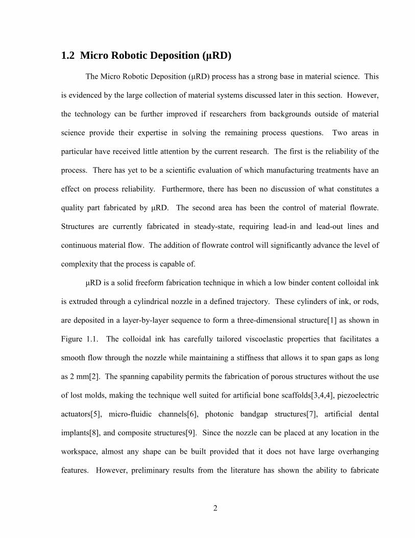
μRD is a solid freeform fabrication technique in which a low binder content colloidal ink

is extruded through a cylindrical nozzle in a defined trajectory. These cylinders of ink, or rods,

are deposited in a layer-by-layer sequence to form a three-dimensional structure[1] as shown in

Figure 1.1. The colloidal ink has carefully tailored viscoelastic properties that facilitates a

smooth flow through the nozzle while maintaining a stiffness that allows it to span gaps as long

as 2 mm[2]. The spanning capability permits the fabrication of porous structures without the use

of lost molds, making the technique well suited for artificial bone scaffolds[3,4,4], piezoelectric

actuators[5], micro-fluidic channels[6], photonic bandgap structures[7], artificial dental

implants[8], and composite structures[9]. Since the nozzle can be placed at any location in the

workspace, almost any shape can be built provided that it does not have large overhanging

features. However, preliminary results from the literature has shown the ability to fabricate

3

overhanging features[10], a key step towards allowing the fabrication of complex structures such

as anatomically shaped bone scaffolds.

All μRD systems have four main components: 1) the material system or the colloidal ink,

2) the substrate, 3) the positioning system, and 4) the extrusion system. See the corresponding

list for a short discussion on each.

1. To date, the majority of the research has focused on the material systems, developing

colloidal systems made from materials with a wide array of physical properties. The list

of materials that have been deposited by μRD includes HA[3,11], alumina[1], barium

titanate[12], lead zirconate titanate[5,13], beta tricalcium phosphate (β–TCP)[4],

polyelectrolytes[14,15], dental porcelain[8,16], and carbon black sacrificial material[10].

The research presented here does not attempt to add to this list, but instead improve the

deposition performance of HA inks.

2. The substrate can be any solid, flat material that will not react with the chemicals in the

colloidal inks.

3. To the author’s knowledge, only XYZ robots have been used as the positioning system

for μRD. The requirements on the positioning system are not strict when compared to

high speed and nano-positioning systems. Positioning systems should be able to achieve

end effector velocities of approximately 30 mm/s and have a resolution of approximately

10 μm.

4. There are few different choices for the extrusion system; these choices are discussed in

Chapter 2.

The μRD technology was invented and originally termed Robocasting [1]. At first, the

technology was presented as a ceramic fabrication technique that required no binders and

4

therefore significantly reduced the fabrication time of complex ceramics since there was not a

lengthy binder burnout process. The ink was deposited on a hot plate to quickly evaporate the

solvent and therefore solidify the recently extruded ink. Since then, binders in low

concentrations have been added to the ink formulation to provide the ink with the unique

property of being able to flow easily through the syringe nozzle and immediately set once

outside the nozzle[5,12]. Much of the research activity surrounding this manufacturing

technology has been performed over the past ten years[4,8,9,17] at a variety of university and

government labs.

20mmNozzle

Reservoir

Plunger

LeadScrew

Figure 1.1. μRD system. (a) Robotic positioning system in the Alleyne Research Group lab. (b) Extrusion system used for this research. (c) Schematic of the extrusion process.

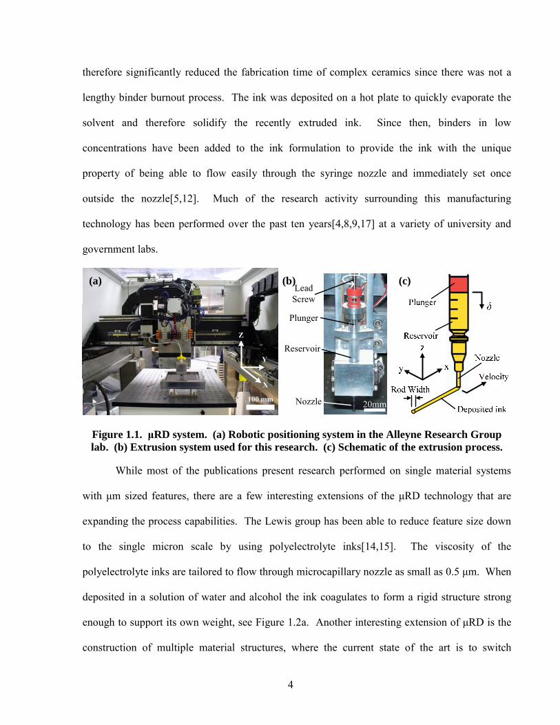
While most of the publications present research performed on single material systems

with μm sized features, there are a few interesting extensions of the μRD technology that are

expanding the process capabilities. The Lewis group has been able to reduce feature size down

to the single micron scale by using polyelectrolyte inks[14,15]. The viscosity of the

polyelectrolyte inks are tailored to flow through microcapillary nozzle as small as 0.5 μm. When

deposited in a solution of water and alcohol the ink coagulates to form a rigid structure strong

enough to support its own weight, see Figure 1.2a. Another interesting extension of μRD is the

construction of multiple material structures, where the current state of the art is to switch

(a) (b) (c)

X

Y

Z

100 mm

5

materials mid-structure. Figure 1.2b shows piezoelectric BaTi03 interlaced with Ni electrodes to

form a piezoelectric actuator[9]. Figure 1.2c shows a structure with long unsupported spans[10].

A sacrificial material supported the overhanging structure as it dried, and then was burned out

with a heating process. Although [9] and [10] show a proof of concept using multiple materials,

the technique is not fully functional. Ideally, the material transitions should be able to be made

mid-layer, instead of mid-structure, for the fabrication of structures more complex than the

simple shapes seen in Figures 1.2b and 1.2c. This capability will require the seamless transition

of materials, a functionality yet unseen in the literature.

Figure 1.2. Examples of structures capable of being produced by μRD. (a) Polyelectrolyte ink structure with μm sized features[15]. (b) Ba-TiO3 interlaced with Ni electrodes[9]. (c)

Structure with long unsupported spans[10].

1.3 Colloidal Science

A complete presentation of the colloidal science behind ceramic colloidal inks for μRD

can be found in a review by Lewis[17]. The purpose of the review presented here is to highlight

a few main topics in colloidal processing: powder processing, particle dispersion, binders, and

flocculation.

1.3.1 Powder Processing

The manufacturing processes that make raw ceramic powder often produce particle

populations that have a rough surface morphology and are agglomerated with other particles[18].

(a)

10 μm

(b) (c)

6

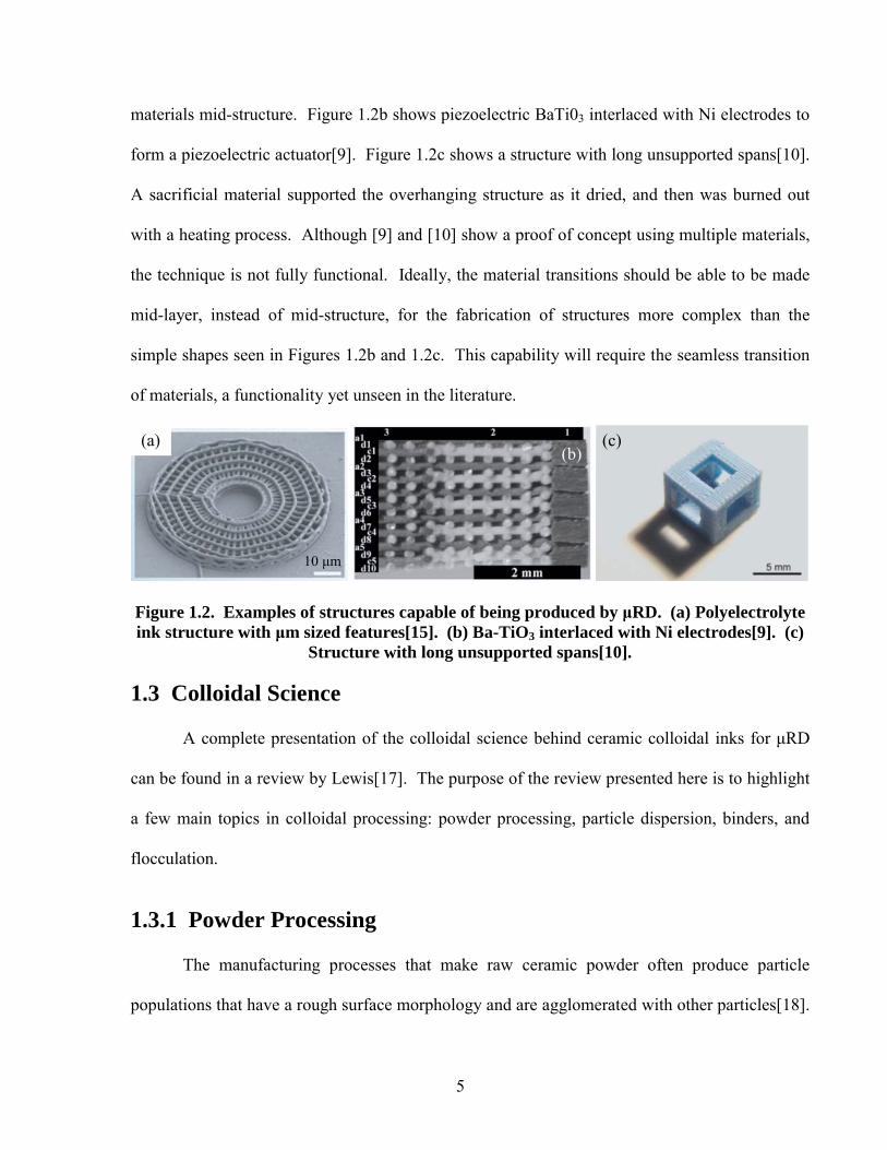
This type of particle distribution is not favorable for colloidal ink fabrication. To change the

rough agglomerated particles into the favorable distribution of smooth monosized particles,

processing steps must be taken. First of these steps is calcining, a heating treatment that

smoothes the surface morphology of ceramic particles. Seen in the images of HA in Figure 1.3,

with calcination time the surface morphology becomes smoother. The calcination process does

cause individual particle to agglomerate. Large particles are unfavorable for deposition because

they can clog deposition nozzles[19] and unfavorable for the finished product because large

particles can lead to irregular grain growth during sintering[18]. Agglomerated particles must be

crushed into their individual constitutive particles through a grinding process. There are a

variety of different processes available[18], but the work in this thesis uses ball milling, a

process in which a solution of powder and solvent is continually agitated with grinding media to

break apart agglomerates.

Figure 1.3. The evolution of hydroxyapatite surface morphology with calcination time.

1.3.2 Particle Dispersion

As stated in Section 1.3.1, it is unfavorable for the colloidal inks to consist of large

agglomerated particles. However, when the powder is added to solution medium van der Waals

forces will pull particles together. Van der Waals forces are ubiquitous weak forces that attract

As-Received 1/2 hour calcination 10 hours calcination

2 μm 2 μm 2 μm

7

all like materials[20]. The potential energy of two spherical particles of diameter a is given

by[18]:

24A

AaUh

−= (1.1)

where A is a materials dependent constant and h is the particle separation distance. These van

der Waals forces never disappear, but the particle surfaces can be modified to prevent the van der

Waals forces from drawings particles together. To that end, dispersing agents are attached to the

particle surface to stabilize the particles from agglomeration. Common dispersing agents use

either electrostatic, steric, or electrosteric forces to stabilize colloids[20]. Since the formulation

in the research presented here uses electrosteric forces, electrosteric dispersants will be briefly

discussed and the other two dispersant types will be left to the reader to research. Electrosteric

dispersant chains have ionizable segments which will attach to the particle surface if the

chemical and physical properties are correct[20]. One physical property that must be satisfied is

that the charge on the dispersant and the particle surface must be opposite for the dispersant to

ionically bond to the surface[12]. The high charge density of the dispersant causes a strong

charge reversal for the particle, creating a solution of strongly repelled particles. Given a strong

enough electrosteric repulsion, the solution is considered stabilized, meaning that the particles

will not agglomerate into large particles. For polyelectrolyte type electrosteric dispersants such

as the one used in this research, the strength of ionization increases with pH[20]. Therefore the

stability of the colloidal solution increases with pH as well.

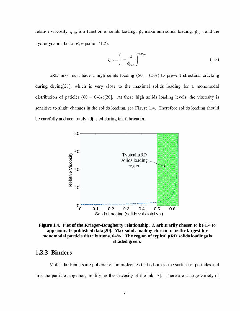
The viscosity of a stable colloidal suspension is primarily dependent on the solids

loading, which is the ratio of suspended solids volume to total suspension volume. The solids

loading dependence of viscosity is best related by the Krieger-Dougherty relationship where

8

relative viscosity, ηrel, is a function of solids loading, φ , maximum solids loading, maxφ , and the

hydrodynamic factor K, equation (1.2).

max

max

1K

rel

φφη

φ

−⎛ ⎞

= −⎜ ⎟⎝ ⎠

(1.2)

μRD inks must have a high solids loading (50 – 65%) to prevent structural cracking

during drying[21], which is very close to the maximal solids loading for a monomodal

distribution of paticles (60 – 64%)[20]. At these high solids loading levels, the viscosity is

sensitive to slight changes in the solids loading, see Figure 1.4. Therefore solids loading should

be carefully and accurately adjusted during ink fabrication.

0 0.1 0.2 0.3 0.4 0.5 0.60

20

40

60

80

Solids Loading (solids vol / total vol)

Rel

ativ

e V

isco

sity

Figure 1.4. Plot of the Krieger-Dougherty relationship. K arbitrarily chosen to be 1.4 to approximate published data[20]. Max solids loading chosen to be the largest for

monomodal particle distributions, 64%. The region of typical μRD solids loadings is shaded green.

1.3.3 Binders

Molecular binders are polymer chain molecules that adsorb to the surface of particles and

link the particles together, modifying the viscosity of the ink[18]. There are a large variety of

Typical μRD solids loading

region

9

molecular binders commercially available. Those interested in the available options can find a

description of the main types in Reed[18]. Only cellulose binders, more specifically methyl

cellulose binders, were used in this research therefore cellulose binders will be discussed here.

Methyl cellulose binders are nonionic binders treated to substitute some of the OH groups in the

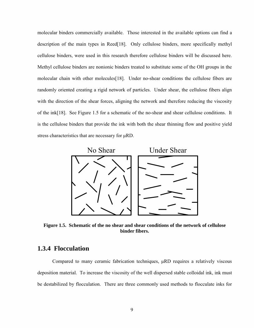
molecular chain with other molecules[18]. Under no-shear conditions the cellulose fibers are

randomly oriented creating a rigid network of particles. Under shear, the cellulose fibers align

with the direction of the shear forces, aligning the network and therefore reducing the viscosity

of the ink[18]. See Figure 1.5 for a schematic of the no-shear and shear cellulose conditions. It

is the cellulose binders that provide the ink with both the shear thinning flow and positive yield

stress characteristics that are necessary for μRD.

No Shear Under Shear

Figure 1.5. Schematic of the no shear and shear conditions of the network of cellulose binder fibers.

1.3.4 Flocculation

Compared to many ceramic fabrication techniques, μRD requires a relatively viscous

deposition material. To increase the viscosity of the well dispersed stable colloidal ink, ink must

be destabilized by flocculation. There are three commonly used methods to flocculate inks for

10

μRD: adding nonadsorbed polymers to disrupt the stability[3,20], adding salt solutions to “mask”

the charge on the dispersant chains[12], or decrease the pH to inhibit the dispersant

adsorption[2]. Some ink formulations use a combination of the techniques, such as the research

presented here which uses a combination of adding nonadsorbed polymers and decreasing the

pH. The flocculation step must be performed carefully or else the ink will become irreversibly

destabilized because the attractive van der Waals forces will dominate the repulsive forces from

the dispersants[20].

1.4 Volumetric Flowrate Control

There is interest in precisely controlling the flow of colloidal inks in μRD to enable the

fabrication of more complex structures; however the precise modulation of ink flow is limited.

Instead, μRD typically uses long lead-in and lead-out lines with a continuous flowrate to build

single material structures. While this method works well for applications that only require one

material, it is inadequate for applications requiring multiple materials. Possible structures could

be artificial bone scaffolds with multiple domains of material properties and near-net shape

scaffolds. Bone scaffolds with multiple material domains could be constituted of a domain of

low porosity to provide material strength and a domain of high porosity to provide high material

surface area for bone cell attachment or improved protein delivery[22], Figure 1.6b. Near-net

shape scaffolds would consist of the build material and a sacrificial material to support

overhanging features in an anatomically shaped structure, Figure 1.6c.

11

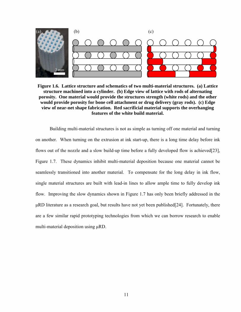
Figure 1.6. Lattice structure and schematics of two multi-material structures. (a) Lattice structure machined into a cylinder. (b) Edge view of lattice with rods of alternating

porosity. One material would provide the structures strength (white rods) and the other would provide porosity for bone cell attachment or drug delivery (gray rods). (c) Edge view of near-net shape fabrication. Red sacrificial material supports the overhanging

features of the white build material.

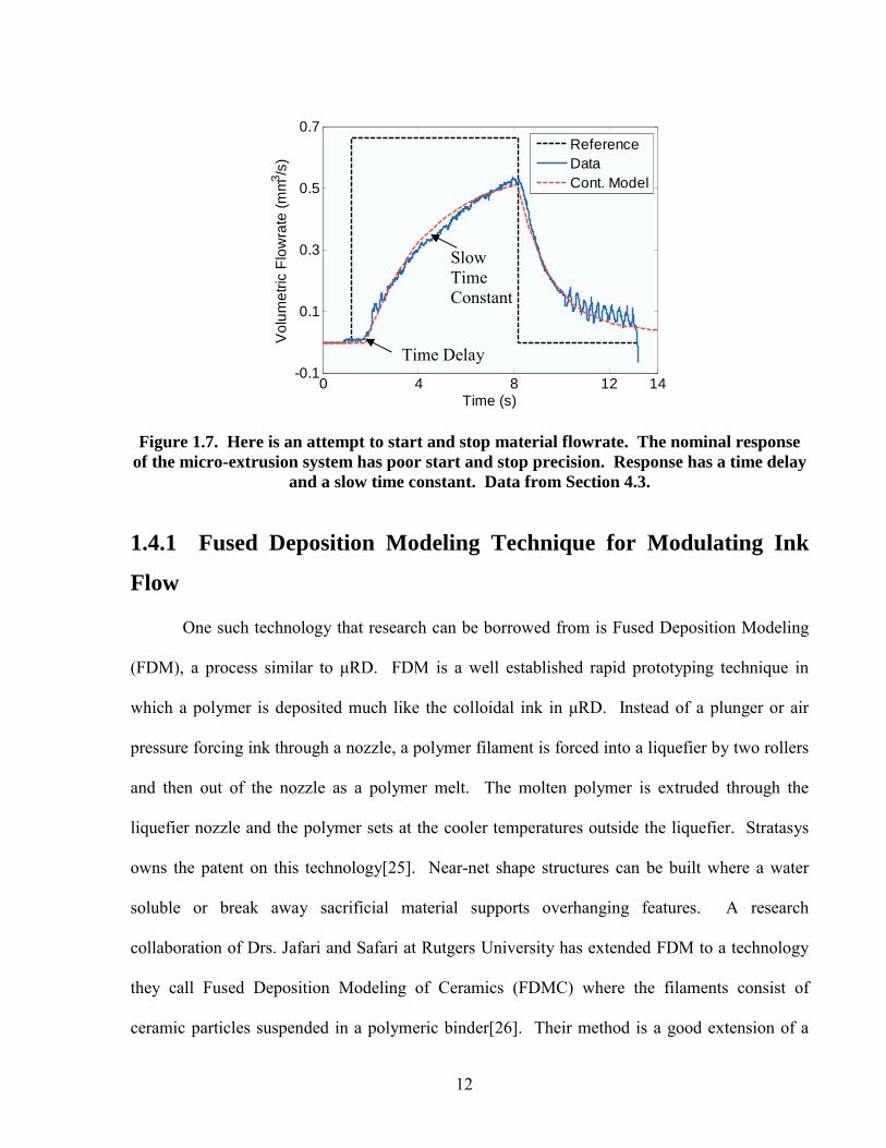
Building multi-material structures is not as simple as turning off one material and turning

on another. When turning on the extrusion at ink start-up, there is a long time delay before ink

flows out of the nozzle and a slow build-up time before a fully developed flow is achieved[23],

Figure 1.7. These dynamics inhibit multi-material deposition because one material cannot be

seamlessly transitioned into another material. To compensate for the long delay in ink flow,

single material structures are built with lead-in lines to allow ample time to fully develop ink

flow. Improving the slow dynamics shown in Figure 1.7 has only been briefly addressed in the

μRD literature as a research goal, but results have not yet been published[24]. Fortunately, there

are a few similar rapid prototyping technologies from which we can borrow research to enable

multi-material deposition using μRD.

(a) (b) (c)

2 mm

12

0 4 8 12 14-0.1

0.1

0.3

0.5

0.7

Time (s)

Vol

umet

ric F

low

rate

(mm

3 /s)

ReferenceDataCont. Model

Figure 1.7. Here is an attempt to start and stop material flowrate. The nominal response of the micro-extrusion system has poor start and stop precision. Response has a time delay

and a slow time constant. Data from Section 4.3.

1.4.1 Fused Deposition Modeling Technique for Modulating Ink

Flow

One such technology that research can be borrowed from is Fused Deposition Modeling

(FDM), a process similar to μRD. FDM is a well established rapid prototyping technique in

which a polymer is deposited much like the colloidal ink in μRD. Instead of a plunger or air

pressure forcing ink through a nozzle, a polymer filament is forced into a liquefier by two rollers

and then out of the nozzle as a polymer melt. The molten polymer is extruded through the

liquefier nozzle and the polymer sets at the cooler temperatures outside the liquefier. Stratasys

owns the patent on this technology[25]. Near-net shape structures can be built where a water

soluble or break away sacrificial material supports overhanging features. A research

collaboration of Drs. Jafari and Safari at Rutgers University has extended FDM to a technology

they call Fused Deposition Modeling of Ceramics (FDMC) where the filaments consist of

ceramic particles suspended in a polymeric binder[26]. Their method is a good extension of a

Time Delay

Slow Time Constant

13

well proven technology. However, they must use binder concentrations that are much higher

than μRD; leading to longer binder burnout periods and lower density structures.

Stratasys System

Stratasys manufactures FDM systems for use in industry and academia. Because they are

a private company, the method by which they control the transitions between materials is not

well published. The best insight into their process is from a patent[25]. Here they control the

filament feedrate with step inputs, Figure 1.8a. Similar to the results seen in Figure 1.7, the

volumetric flowrate response at the deposition tip is first order with a time delay, Figure 1.8b.

Stratasys over-steps the roller speed at startup (pre-pump phase), and under steps the roller speed

at material termination (suck-back phase). To precisely start and stop ink flow, the flowrate is

matched with the tip speed of the extrusion mechanism, Figure 1.8c. This technique is run

entirely in open loop with the timing of ink flow and tip speed being purely empirical.

This is a simple idea and apparently it is well proven if this is indeed what Stratasys uses

on their FDM machines. However, colloidal inks are very compressible and vary significantly

from material to material and batch to batch, unlike mass produced polymer filaments that are

more reproducible from well developed quality controls on the process. The irregularities in ink

rheology would make the empirical matching of flowrate and deposition speed for every new ink

troublesome. Instead, a quick procedure at the beginning of part fabrication, or on the first trial

of a new batch of ink, to properly identify the flowrate dynamics would be favorable. A quick

identification procedure could be coupled with Stratasys’s empirical timing of flowrates and

deposition speed to provide further deposition accuracy.

14

Figure 1.8. Timing diagram for starting and stopping of polymer flow in the Stratasys FDM[25].

Rutgers System

Two researchers at Rutgers have extended FDM by exchanging the polymer

filaments for filaments consisting of ceramic material suspended in a polymeric binder, naming

the new system Fused Deposition Modeling of Ceramics (FDMC). In the majority of their

research, the method of turning on and off the ink flow is not specified. However, they do

mention that the start/stop problem, consisting of the long time delay and slow response of the

Time Delay

First Order Exponential Response

15

material flowrate, is a major problem and they can address the problem with trajectory

planning[27]. Trajectory planning is simply starting or stopping the deposition early and using

trajectories that minimize the number of start-stop occurrences.

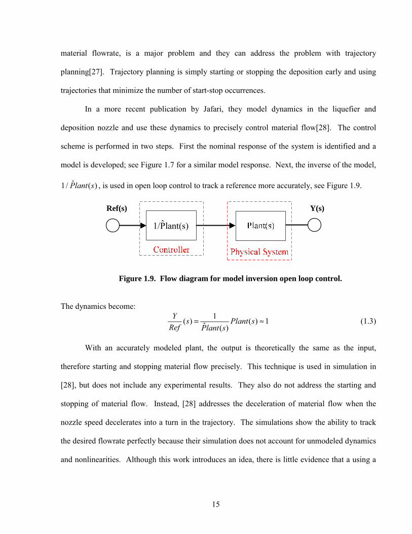
In a more recent publication by Jafari, they model dynamics in the liquefier and

deposition nozzle and use these dynamics to precisely control material flow[28]. The control

scheme is performed in two steps. First the nominal response of the system is identified and a

model is developed; see Figure 1.7 for a similar model response. Next, the inverse of the model,

ˆ1/ ( )Plant s , is used in open loop control to track a reference more accurately, see Figure 1.9.

Figure 1.9. Flow diagram for model inversion open loop control.

The dynamics become:

1( ) ( ) 1ˆ ( )Y s Plant s

Ref Plant s= ≈ (1.3)

With an accurately modeled plant, the output is theoretically the same as the input,

therefore starting and stopping material flow precisely. This technique is used in simulation in

[28], but does not include any experimental results. They also do not address the starting and

stopping of material flow. Instead, [28] addresses the deceleration of material flow when the

nozzle speed decelerates into a turn in the trajectory. The simulations show the ability to track

the desired flowrate perfectly because their simulation does not account for unmodeled dynamics

and nonlinearities. Although this work introduces an idea, there is little evidence that a using a

Ref(s) Y(s)

ˆ1/Plant(s)

16

linear model inversion feedforward controller will successfully control the extrusion of ink with

uncertain dynamics.

1.4.2 Flowrate Dynamics Modeling and Iterative Learning Control

In Chapter 4, we propose a vision-based Iterative Learning Control (ILC) procedure to

both identify the fluid dynamics in the extruder and control the extrusion for precise deposition.

This chapter combines research from fluid dynamics, extrusion system modeling, machine

vision, and Iterative Learning Control (ILC).

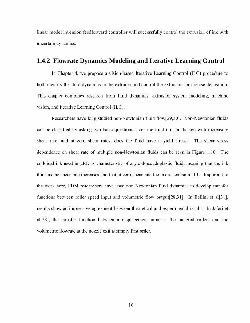
Researchers have long studied non-Newtonian fluid flow[29,30]. Non-Newtonian fluids

can be classified by asking two basic questions; does the fluid thin or thicken with increasing

shear rate, and at zero shear rates, does the fluid have a yield stress? The shear stress

dependence on shear rate of multiple non-Newtonian fluids can be seen in Figure 1.10. The

colloidal ink used in μRD is characteristic of a yield-pseudoplastic fluid, meaning that the ink

thins as the shear rate increases and that at zero shear rate the ink is semisolid[10]. Important to

the work here, FDM researchers have used non-Newtonian fluid dynamics to develop transfer

functions between roller speed input and volumetric flow output[28,31]. In Bellini et al[31],

results show an impressive agreement between theoretical and experimental results. In Jafari et

al[28], the transfer function between a displacement input at the material rollers and the

volumetric flowrate at the nozzle exit is simply first order.

17

Figure 1.10. Non-Newtonian Fluids. Shear thinning fluids are termed pseudoplastic and shear thickening fluids are termed dilatant[29].

Chapter 4 proposes that ILC can be used to improve the modulation of ink flowrate. ILC

has been used primarily to improve tracking of reference signals for robots in repetitive

processes. The technology has rarely been applied to a process in which the output variable is

the end product performance, not a tracking error[32]. Similar to [32], in Chapter 4 the goal is to

monitor the end product performance, volumetric flowrate in this case, and iteratively modify the

control signal to achieve the desired flowrate. A typical ILC algorithm, equation (1.4)[33], is

used to prove that basic ILC can successfully modulate a process output that is monitored using a

vision system.

1( ) ( ) ( ) ( ) ( 1)j j ju k Q q u k L q e k+ ⎡ ⎤= + +⎣ ⎦ (1.4)

In equation (1.4), j is the iteration number and k is the discrete time index number. Q(q) is the

Q-filter which is typically a low-pass filter that dampens high frequency signal content for a

smoother control signal, u. ej(k+1) is the error term of the current iteration of the next index in

18

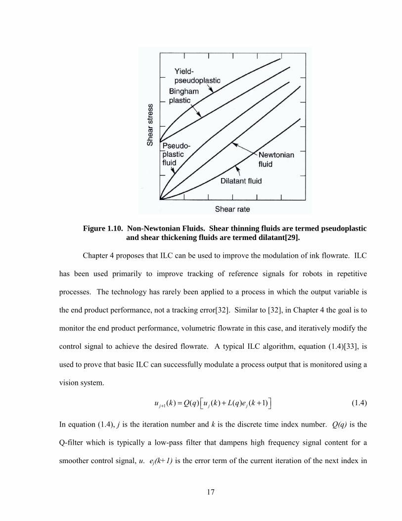
time. L(q) is the learning function that generally has one of the following forms: Proportional

Derivative (PD), Model Inversion, H∞, or Quadratically Optimal[33]. Chapter 4 utilizes the PD

and Model Inversion forms of the learning controller. A visual representation of the ILC

algorithm is displayed in Figure 1.11, where after each iteration the error signal and the control

signal, ej(k+1) and uj(k) respectively, are fed into the ILC algorithm to produce the control signal

for the next iteration, uj+1(k).

Figure 1.11. Visual representation of the ILC algorithm[33].

1.5 Artificial Bone Scaffolds

The research presented in this thesis aims to improve μRD in general. However, the

target application is focused specifically on artificial bone scaffolds. With bone scaffolding in

mind, the only material used was hydroxyapatite, a common artificial bone scaffold material[34],

and many of the structures that were built had the same architecture as common scaffold

structures[35]. For a successful artificial bone scaffold, what is most important is the material

19

and architecture of the final product[34]. Therefore the structures that were built were designed

to be potential bone scaffolds.

Ideally, a bone substitute should be, “osteoconductive, osteoinductive, biocompatible,

bio-resorbable, structurally similar to bone, easy to use, and cost effective[36].” A perfect bone

substitute that fulfills all of these requirements has yet to be developed, but these are good goals

to aspire towards. Hydroxyapatite was chosen for this research for a few reasons. It is

biocompatible with native bone because it is stoichiometrically similar to the bone mineral[36].

The load bearing properties can be designed to be similar to trabecular bone[37]. Also, when

fabricated by μRD, the scaffolds have an easily modified macro and micro porosity[11]. The

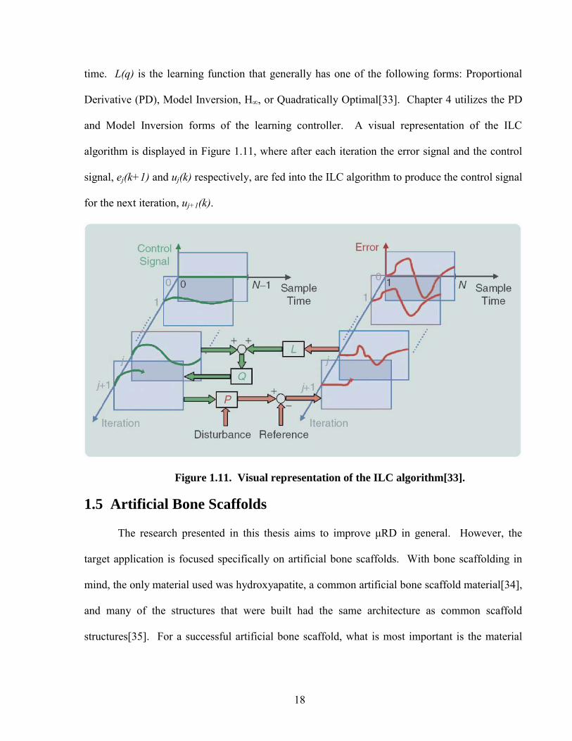
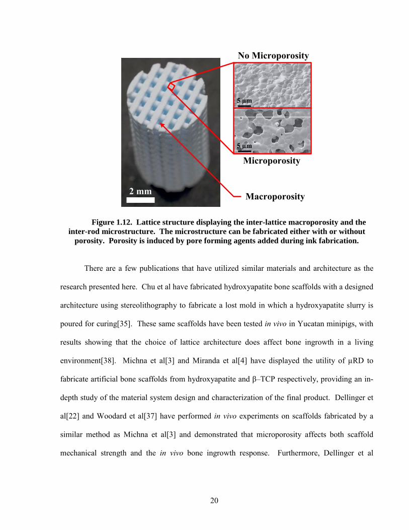
structure most commonly fabricated was the lattice structure, see Figure 1.12. The pore size in

the lattice was carefully chosen to match the size range published as optimal for

osteoconductivity of bone. Although the optimal pore architecture has been disputed, Hing

suggests to design scaffolds for a total porosity of greater than 50 – 60%, pore interconnection

channels of greater than 50 – 100 μm, and a rod porosity of greater than 20%[34]. The first two

suggestions are satisfied by choosing the rod diameter and nozzle trajectory appropriately. The

inter-rod porosity, Figure 1.12, is achieved by inducing porosity by the addition of pore forming

agents, discussed in more detail in Appendix A.

20

5 µm

5 µm

Macroporosity

Microporosity

No Microporosity

2 mm

Figure 1.12. Lattice structure displaying the inter-lattice macroporosity and the inter-rod microstructure. The microstructure can be fabricated either with or without

porosity. Porosity is induced by pore forming agents added during ink fabrication.

There are a few publications that have utilized similar materials and architecture as the

research presented here. Chu et al have fabricated hydroxyapatite bone scaffolds with a designed

architecture using stereolithography to fabricate a lost mold in which a hydroxyapatite slurry is

poured for curing[35]. These same scaffolds have been tested in vivo in Yucatan minipigs, with

results showing that the choice of lattice architecture does affect bone ingrowth in a living

environment[38]. Michna et al[3] and Miranda et al[4] have displayed the utility of μRD to

fabricate artificial bone scaffolds from hydroxyapatite and β–TCP respectively, providing an in-

depth study of the material system design and characterization of the final product. Dellinger et

al[22] and Woodard et al[37] have performed in vivo experiments on scaffolds fabricated by a

similar method as Michna et al[3] and demonstrated that microporosity affects both scaffold

mechanical strength and the in vivo bone ingrowth response. Furthermore, Dellinger et al

21

displayed the potential of the micropores as drug delivery vessels to bring growth factors directly

to the damaged site that needs new bone growth[22].

1.6 Thesis Contributions

The previous sections served as a broad introduction to the different technological aspects

used in the subsequent chapters. Section 1.2 directly relates to Chapters 2, 3, and 4. Section 1.3

directly relates to Chapter 3. Section 1.4 directly relates to Chapters 2 and 4. Section 1.5

provides background information on the intended application of this research. The following

provides an overall summary of the contributions of the thesis to the literature and an outline of

the subsequent chapters.

Chapter 2:

An outline of the deposition procedure is presented. The main contribution to the field of

μRD is the streamlining of the deposition process by centrifuging syringes for air bubble

removal. Previously, syringes were manually tapped, which was a time consuming and

strenuous process. The centrifugal method significantly decreases this processes time and effort,

and has not displayed any adverse effects.

Chapter 3:

This chapter is an intensive study of the deposition process for the μRD of macro-sized

structures with micro-sized features. To the best of the authors’ knowledge, this is the first time

that a scientific study has been used to determine which manufacturing variables affect μRD

process reliability. A design of experiments approach determines that calcination time, nozzle

size, and deposition speed all have a significant affect on lattice quality. Correlations between

the manufacturing parameters and part quality metrics are presented and possible mechanisms

that explain the correlations are discussed.

22

Chapter 4:

The research here combines ILC and machine vision to modulate ink flowrate in μRD.

This work is one of the first to apply ILC directly to a process and the first to our knowledge to

incorporate machine vision within the ILC framework. The results show that ILC can be used to

improve flowrate modulation in μRD and that the choice of the learning controller used has an

effect on the system performance.

Chapter 5:

This chapter presents a thesis summary, conclusions, and future work.

Nomenclature

Symbol Description Units A Hamaker Constant J a Particle Diameter nm e Error Signal - h Particle Separation Distance nm j Iteration Index Iterations K Hydrodynamic Factor unitless k Time Step Index Time StepsL(q) Learning Filter - Plant(s) Plant Transfer Function - Q(q) Q-Filter - Ref(s) Reference - u Control Signal - UA van der Waals Potential Energy J Y(s) Output - ηrel Relative Viscosity unitless φ Solids Loading unitless φmax Maximum Solids Loading unitless

Table 1.1. Nomenclature

References

[1] Cesarano, J. , Segalman, R., and Calvert, P., Robocasting provides moldless fabrication

from slurry deposition Ceramic Industry, vol. 148, pp. 94-102, Apr, 1998.

23

[2] Smay, J. E., Cesarano III, J., and Lewis, J. A., Colloidal Inks for Directed Assembly of 3-D Periodic Structures Langmuir, vol. 18, pp. 5429-5437, 2002.

[3] Michna, S., Wu, W., and Lewis, J. A., Concentrated hydroxyapatite inks for direct-write assembly of 3-D periodic scaffolds Biomaterials, vol. 26, pp. 5632-5639, 2005.

[4] Miranda, P., Saiz, E., Gryn, K., and Tomsia, A. P., Sintering and Robocasting of β-Tricalcium Phosphate Scaffolds for Orthopaedic Applications Acta Biomaterialia, vol. 2, pp. 457-466, 2006.

[5] Smay, J. E., Cesarano III, J., Tuttle, B. A., and Lewis, J. A., Directed Colloidal Assembly of Linear and Annular Lead Zirconate Titanate Arrays Journal of the American Ceramic Society, vol. 87, pp. 293-295, 2004.

[6] Therriault, D., White, S. R., and Lewis, J. A., Chaotic mixing in three-dimensional microvascular networks fabricated by direct-write assembly Nature Materials, vol. 2, pp. 265-271, 2003.

[7] Gratson, G. M., Garcia-Santamaria, F., Lousse, V., Xu, M., Fan, S., Lewis, J. A., and Braun, P. V., Direct-Write Assembly of Three-Dimensional Photonic Crystals: Conversion of Polymer Scaffolds to Silicon Hollow-Woodpile Structures Advanced Materials , vol. 18, pp. 461-465, 2006.

[8] Wang, J., Shaw, L. L., and Cameron, T. B., Solid Freeform Fabrication of Permanent Dental Restorations via Slurry Micro-Extrusion Journal of the American Ceramic Society, vol. 89, pp. 346-349, 2006.

[9] Smay, J. E., Nadkarni, S. S., and Xu, J., Direct Writing of Dielectric Ceramics and Base Metal Electrodes International Journal of Applied Ceramic Technology, vol. 4, pp. 47-52, 2007.

[10] Lewis, J. A., Smay, J. E., Stuecker, J., and Cesarano III, J., Direct Ink Writing of Three-Dimensional Ceramic Structures Journal of the American Ceramic Society, vol. 89, pp. 3599-3609, 2006.

[11] Cesarano III, J., Dellinger, J. G., Saavedra, M. P., Gill, D. D., Jamison, R. D., Grosser, B. A., Sinn-Hanlon, J. M., and Goldwasser, M. S., Customization of Load-Bearing Hydroxyapatite Lattice Scaffolds International Journal of Applied Ceramic Technology, vol. 2, pp. 212-220, 2005.

[12] Li, Q. and Lewis, J. A., Nanoparticle Inks for Directed Assembly of Three-Dimensional Periodic Structures Advanced Materials, vol. 12, pp. 1639-1643, 2003.

[13] Tuttle, B. A., Smay, J. A., Cesarano III, J., Voigt, J. A., Scofield, T. W., and Olson, W. R., Robocast Pb(Zr0.095Ti0.05)O3 Ceramic Monoliths and Composites Journal of the American Ceramic Society, vol. 84, pp. 872-874, 2001.

[14] Gratson, G. M. and Lewis, J. A., Phase Behavior and Rheological Properties of

24

Polyelectrolyte Inks for Direct-Write Assembly Langmuir, vol. 21, pp. 457-464, 2005.

[15] Gratson, G. M., Xu, M., and Lewis, J. A., Direct writing of three-dimensional webs Nature, vol. 428, pp. 386, 2004.

[16] Wang, J. and Shaw, L. L., Rheological and extrusion behavior of dental porcelain slurries for rapid prototyping applications Materials Science and Engineering A, vol. 397, pp. 314-321, 2005.

[17] Lewis, J. A., Direct Ink Writing of 3D Functional Materials Advanced Functional Materials, vol. 16, pp. 2193-2204, 2006.

[18] Reed, J. S. Introduction to the Principles of Ceramic Processing, United States of America : John Wiley & Sons, Inc., 1987.

[19] Wyss, H. M. , Blair, D. L., Morris, J. F., Stone, H. A., and Weitz, D. A., Mechanism for clogging of microchannels Physical Review E, vol. 74 , pp. 061402, 2006.

[20] Lewis, J. A., Colloidal Processing of Ceramics Journal of the American Ceramic Society, vol. 83, pp. 2341-2359, 2000.

[21] Cesarano III, J., "A Review of Robocasting Technology ," Materials Research Society Symposium Proceedings, Boston, MA, pp. 133-139, 1999.

[22] Dellinger, J. G., Development of Model Hydroxyapatite Bone Scaffolds with Multiscale Porosity for Potential Load Bearing Applications 2005. University of Illinois at Urbana-Champaign.

[23] Hoelzle, D. J., Alleyne, A. G., and Wagoner Johnson, A. J., Iterative Learning Control for Robotic Deposition Using Machine Vision Submitted to ACC 2008, vol. 2008.

[24] Lewis, J. A., Direct-Write Assembly of Ceramics from Colloidal Inks Current Opinion in Solid State and Materials Science, vol. 6 , pp. 245-250, 2002.

[25] Comb, J. W. , Leavitt, P. J., and Rapoport, E., inventors. I. Statasys, assignee. Velocity Profiling in an Extrusion Apparatus. United States. no. 6054077, Apr 25, 2000.

[26] McNulty, T. F., Shanefield, D. J., Danforth, S. C., and Safari, A., Dispersion of Lead Zirconate Titanate for Fused Deposition of Ceramics Journal of the American Ceramic Society, vol. 82, pp. 1757-1760, 1999.

[27] Bouhal, A., Jafari, M. A., Han, W.-B., and Fang, T., Tracking Control and Trajectory Planning in Layered Manufacturing Applications IEEE Transactions on Industrial Electronics, vol. 46, pp. 445-451, 1999.

[28] Han, W. and Jafari, M. A., Coordination Control of Positioning and Deposition in Layered Manufacturing IEEE Transactions on Industrial Electronics, vol. 54, pp. 651-659, Feb, 2007.

25

[29] Chhabra, R. and Richardson, J., Non-Newtonian Flow in the Process Industries, 5-161, 1999. Butterworth-Heinemann. Oxford, UK.

[30] Bohme, G., non-newtonian fluid mechanics Anonymouspp. 591987. North-Holland series in applied mathematics and mechanics. Elsevier Science Publishers B.V. Amsterdam, Netherlands.

[31] Bellini, A. , Güçeri, S., and Bertoldi, M., Liquefier Dynamics in Fused Deposition Journal of Manufacturing Science and Engineering, vol. 126, pp. 237-246, 2004.

[32] Lee, K. S. and Lee, J. H., Iterative Learning Control-Based Batch Process Control Technique for Integrated Control of End Product Properties and Transient Profiles of Process Variables Journal of Process Control, vol. 13, pp. 607-621, 2003.

[33] Bristow, D. A., Tharayil, M., and Alleyne, A. G., A survey of Iterative Learning Control IEEE Control Systems Magazine, vol. pp. 96-114, Jun, 2006.

[34] Hing, K. A. , Bioceramic Bone Graft Substitutes: Influence of Porosity and Chemistry International Journal of Applied Ceramic Technology, vol. 2, pp. 184-199, 2005.

[35] Chu, T.-M. G., Halloran, J. W., Hollister, S. J., and Feinberg, S. E., Hydroxyapatite Implants with Designed Internal Architecture Journal of Material Science: Materials in Medicine, vol. 12, pp. 471-478, 2001.

[36] Giannoudis, P. V., Dinopoulos, H., and Tsiridis, E., Bone Substitutes: An Update International Journal of the Care of the Injured, vol. 36S, pp. S20-S272005.

[37] Woodard, J. R., Hilldore, A. J., Lan, S. K., Park, C. J., Morgan, A. W., Eurell, J. A. C., Clark, S. G., Wheeler, M. B., Jamison, R. D., and Wagoner Johnson, A. J., The Mechanical Properties and Osteoconductivity of Hydroxyapatite Bone Scaffolds with Multi-Scale Porosity Biomaterials, vol. 28, pp. 45-54, 2007.

[38] Chu, T.-M. G., Orton, D. G., Hollister, S. J., Feinberg, S. E., and Halloran, J. W., Mechanical and in vivo performance of hydroxyapatite implants with controlled architectures Biomaterials, vol. 23, pp. 1283-1293, 2002.

26

Chapter 2 Deposition

2.1 Introduction

Micro Robotic Deposition (μRD) systems have four main components: the colloidal ink,

the substrate, the positioning system, and the extrusion system. In this chapter, the positioning

system and extrusion system used for the research presented in Chapters 3 and 4 will be

described. The positioning system positions the extrusion system in three-dimensional space

while the extrusion system extrudes the colloidal ink. Three-dimensional structures are

fabricated by coordinating the actions of the positioning and extrusions systems.

While the positioning system can take on many forms and still provide the necessary

performance, the choice of extrusion system is more deterministic of the process performance.

There are two basic types of ink extrusion, controlled displacement and controlled pressure[1].

In controlled displacement extrusion, the displacement of a plunger is controlled and the plunger

in turn extrudes the ink through the syringe nozzle. In controlled pressure extrusion, a controlled

pressure is applied to the ink reservoir that in turn extrudes the ink. Controlled displacement is

the most common ink extrusion method for large rod sizes (100 μm – 1 mm) because the

controlled pressure method is more sensitive to slight variations in ink rheology[1]. However, at

smaller rod sizes, a mechanical system cannot produce the fine displacement resolutions required

to continuously extrude the ink and a controlled pressure system must be used instead[2]. A

controlled pressure system consists of a pressure regulator and air tubing attached to the reservoir

27

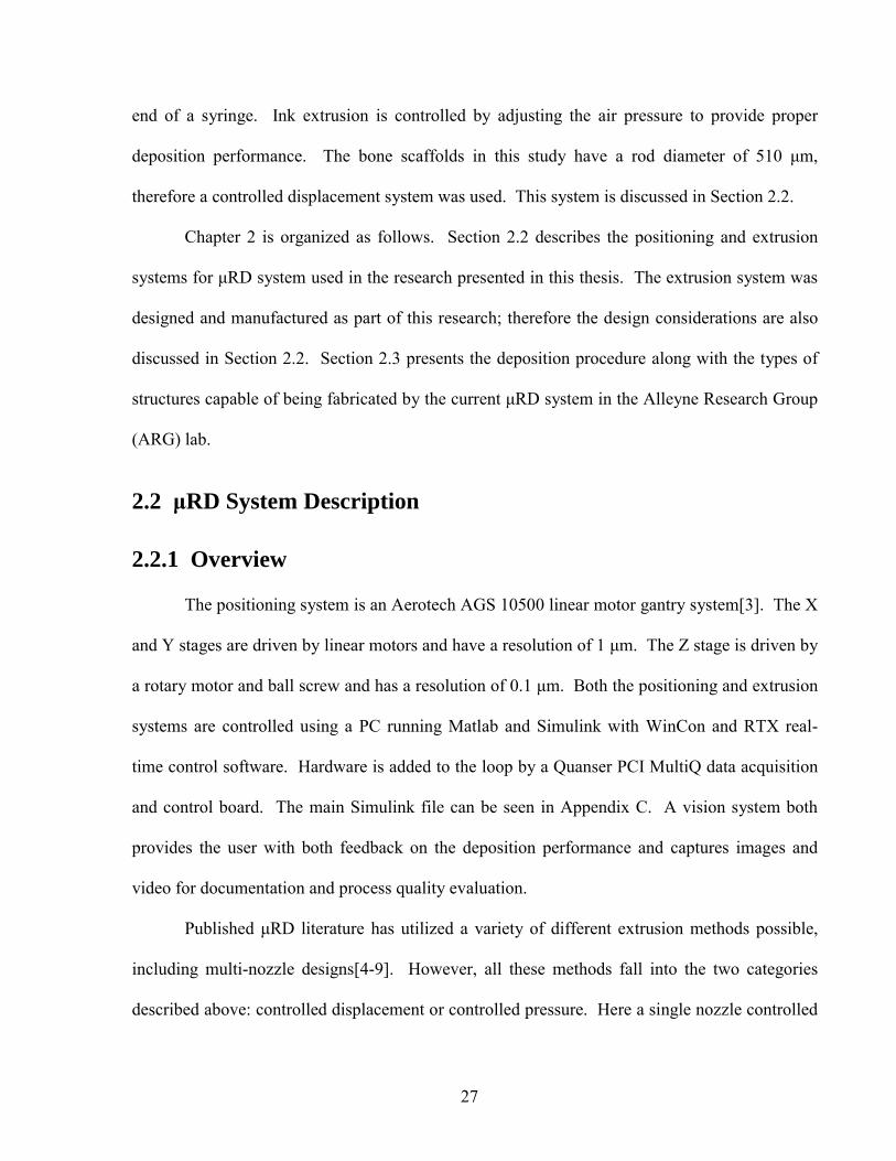
end of a syringe. Ink extrusion is controlled by adjusting the air pressure to provide proper

deposition performance. The bone scaffolds in this study have a rod diameter of 510 μm,

therefore a controlled displacement system was used. This system is discussed in Section 2.2.

Chapter 2 is organized as follows. Section 2.2 describes the positioning and extrusion

systems for μRD system used in the research presented in this thesis. The extrusion system was

designed and manufactured as part of this research; therefore the design considerations are also

discussed in Section 2.2. Section 2.3 presents the deposition procedure along with the types of

structures capable of being fabricated by the current μRD system in the Alleyne Research Group

(ARG) lab.

2.2 μRD System Description

2.2.1 Overview

The positioning system is an Aerotech AGS 10500 linear motor gantry system[3]. The X

and Y stages are driven by linear motors and have a resolution of 1 μm. The Z stage is driven by

a rotary motor and ball screw and has a resolution of 0.1 μm. Both the positioning and extrusion

systems are controlled using a PC running Matlab and Simulink with WinCon and RTX real-

time control software. Hardware is added to the loop by a Quanser PCI MultiQ data acquisition

and control board. The main Simulink file can be seen in Appendix C. A vision system both

provides the user with both feedback on the deposition performance and captures images and

video for documentation and process quality evaluation.

Published μRD literature has utilized a variety of different extrusion methods possible,

including multi-nozzle designs[4-9]. However, all these methods fall into the two categories

described above: controlled displacement or controlled pressure. Here a single nozzle controlled

28

displacement extrusion system was chosen for this research because the basic bone scaffolds

under consideration required only one material and the feature size of interest can be more

consistently deposited with a controlled displacement system. Controlled displacement extrusion

is shown schematically in Figure 1.1c. Here a plunger is driven by a distance of either positive

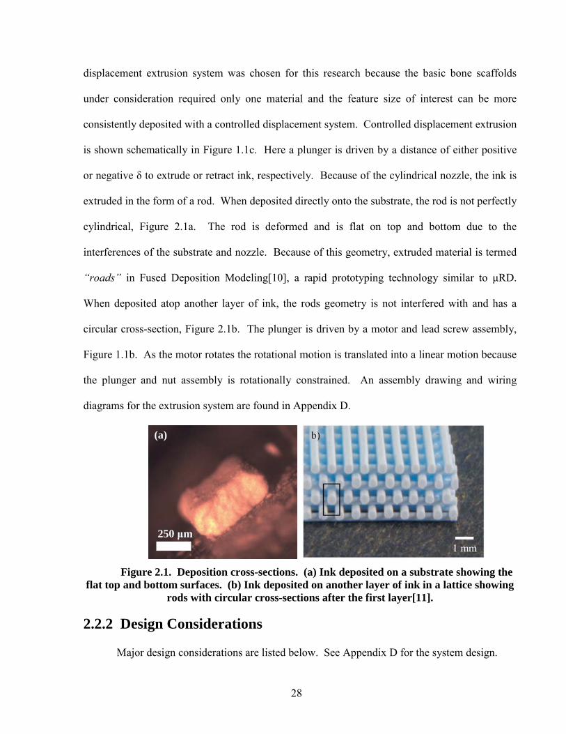
or negative δ to extrude or retract ink, respectively. Because of the cylindrical nozzle, the ink is

extruded in the form of a rod. When deposited directly onto the substrate, the rod is not perfectly

cylindrical, Figure 2.1a. The rod is deformed and is flat on top and bottom due to the

interferences of the substrate and nozzle. Because of this geometry, extruded material is termed

“roads” in Fused Deposition Modeling[10], a rapid prototyping technology similar to μRD.

When deposited atop another layer of ink, the rods geometry is not interfered with and has a

circular cross-section, Figure 2.1b. The plunger is driven by a motor and lead screw assembly,

Figure 1.1b. As the motor rotates the rotational motion is translated into a linear motion because

the plunger and nut assembly is rotationally constrained. An assembly drawing and wiring

diagrams for the extrusion system are found in Appendix D.

Figure 2.1. Deposition cross-sections. (a) Ink deposited on a substrate showing the

flat top and bottom surfaces. (b) Ink deposited on another layer of ink in a lattice showing rods with circular cross-sections after the first layer[11].

2.2.2 Design Considerations

Major design considerations are listed below. See Appendix D for the system design.

250 μm

(a)

29

Motor and Lead Screw Selection: The proper choice of actuation components was the most

important decisions made. The motor selected had adequate torque to extrude the ink and was

compact to save space in the design. The lead screw was selected to provide the smallest lead

possible, yet still have enough thread strength so that the lead screw would not break during

operation.

Syringe Mounting: There are a variety of designs that could affix the syringe to the extrusion

mechanism. For this design, the simplest design was chosen. A clamping system held the

syringe in place by friction. In future designs, it is advisable to add mechanical stops that hold

the syringe up by its wings because the frictional design was not adequate at times.

Extrusion System Attachment: Here a rigid extension was added to move the extrusion system

down and away from the positioning system attachment point. There were already several

existing components mounted on the positioning system that had to be avoided.

Electrical System: Many problems were encountered from system noise because the signal line

ran next to the PWM power line in the cable trays. In future designs, extra attention should be

paid to make sure the signal and power lines are separated as best possible and to ensure proper

grounding. Analog filters had to be added to the signal wire circuitry to attenuate high frequency

noise. Additional shielding in the cable could be used to mitigate noise problems.

Software: The GUI and Simulink diagram were modified to accommodate the new extrusion

system. For normal lattice deposition, Section 2.3, the extruder motor speed is tied in direct

proportion to the positioning system speed to maintain a continuous rod of colloidal ink,

equation (2.1).

2

4Q d vπ= (2.1)

In (2.1) the volumetric flowrate, Q, is a function of nozzle diameter, d, and deposition speed, v.

30

2.3 Deposition Procedure

The step-by-step deposition procedure can be found in Appendix C. New to the μRD

technology is the centrifugal syringe de-airing technique described in this procedure. Previously,

ink was loaded into a syringe and then the syringe was manually “tapped” against a hard object

to shuffle the entrapped air bubbles out of suspension. Although this technique worked, it was

labor intensive and not ideal for a mass manufacturing environment. Instead this chapter

presents an improved de-airing technique that is effective, fast, and easy. Ink is loaded into the

syringe but instead of attaching a vacuum line to the syringe and tapping it, the capped syringe is

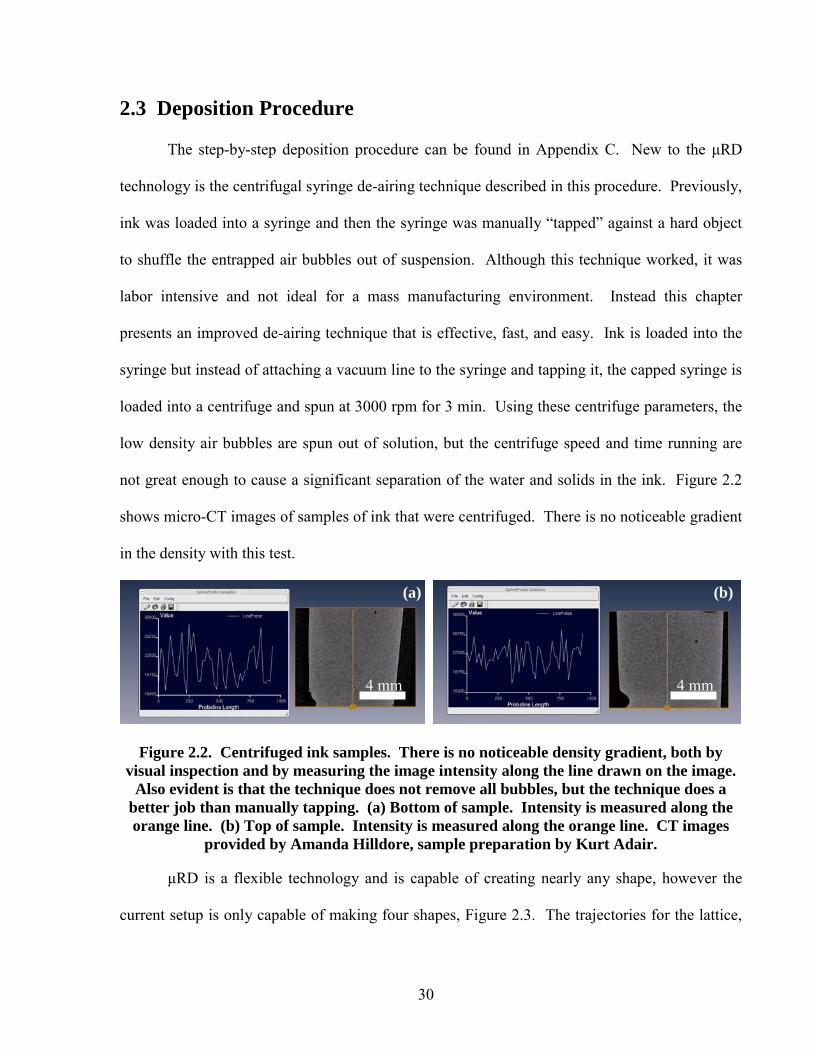
loaded into a centrifuge and spun at 3000 rpm for 3 min. Using these centrifuge parameters, the

low density air bubbles are spun out of solution, but the centrifuge speed and time running are

not great enough to cause a significant separation of the water and solids in the ink. Figure 2.2

shows micro-CT images of samples of ink that were centrifuged. There is no noticeable gradient

in the density with this test.

Figure 2.2. Centrifuged ink samples. There is no noticeable density gradient, both by visual inspection and by measuring the image intensity along the line drawn on the image.

Also evident is that the technique does not remove all bubbles, but the technique does a better job than manually tapping. (a) Bottom of sample. Intensity is measured along the orange line. (b) Top of sample. Intensity is measured along the orange line. CT images

provided by Amanda Hilldore, sample preparation by Kurt Adair.

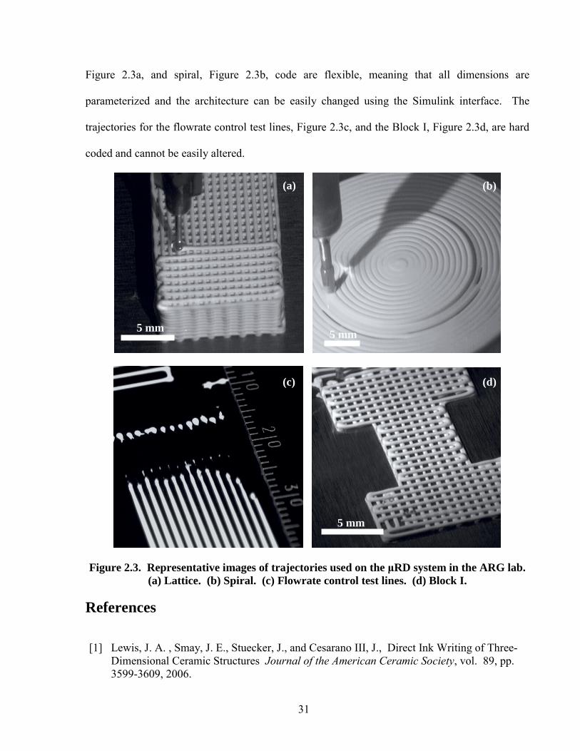
μRD is a flexible technology and is capable of creating nearly any shape, however the

current setup is only capable of making four shapes, Figure 2.3. The trajectories for the lattice,

(a) (b)

4 mm 4 mm

31

Figure 2.3a, and spiral, Figure 2.3b, code are flexible, meaning that all dimensions are

parameterized and the architecture can be easily changed using the Simulink interface. The

trajectories for the flowrate control test lines, Figure 2.3c, and the Block I, Figure 2.3d, are hard

coded and cannot be easily altered.

Figure 2.3. Representative images of trajectories used on the μRD system in the ARG lab. (a) Lattice. (b) Spiral. (c) Flowrate control test lines. (d) Block I.

References

[1] Lewis, J. A. , Smay, J. E., Stuecker, J., and Cesarano III, J., Direct Ink Writing of Three-

Dimensional Ceramic Structures Journal of the American Ceramic Society, vol. 89, pp. 3599-3609, 2006.

5 mm

5 mm

(a)

(c) (d)

(b)

5 mm

32

[2] Gratson, G. M., Xu, M., and Lewis, J. A., Direct writing of three-dimensional webs Nature, vol. 428, pp. 386, 2004.

[3] Bristow, D. and Alleyne, A., A Manufacturing System for Microscale Robotic Deposition, Proceedings of the American Controls Conference, 2003.

[4] Lewis, J. A. , Direct-Write Assembly of Ceramics from Colloidal Inks Current Opinion in Solid State and Materials Science, vol. 6, pp. 245-250, 2002.

[5] Smay, J. E., Nadkarni, S. S., and Xu, J., Direct Writing of Dielectric Ceramics and Base Metal Electrodes International Journal of Applied Ceramic Technology, vol. 4, pp. 47-52, 2007.

[6] Cesarano, J. , Segalman, R., and Calvert, P., Robocasting provides moldless fabrication from slurry deposition Ceramic Industry, vol. 148, pp. 94-102, Apr, 1998.

[7] Gratson, G. M., Garcia-Santamaria, F., Lousse, V., Xu, M., Fan, S., Lewis, J. A., and Braun, P. V., Direct-Write Assembly of Three-Dimensional Photonic Crystals: Conversion of Polymer Scaffolds to Silicon Hollow-Woodpile Structures Advanced Materials , vol. 18, pp. 461-465, 2006.

[8] Miranda, P., Saiz, E., Gryn, K., and Tomsia, A. P., Sintering and Robocasting of β-Tricalcium Phosphate Scaffolds for Orthopaedic Applications Acta Biomaterialia, vol. 2, pp. 457-466, 2006.

[9] Wang, J., Shaw, L. L., and Cameron, T. B., Solid Freeform Fabrication of Permanent Dental Restorations via Slurry Micro-Extrusion Journal of the American Ceramic Society, vol. 89, pp. 346-349, 2006.

[10] Han, W., Jafari, M. A., Danforth, S. C., and Safari, A., Tool Path-Based Deposition Planning in Fused Deposition Processes Transactions of the ASME: Journal of Manufacturing Science and Engineering, vol. 124, pp. 462-472, 2002.

[11] Dellinger, J. G., Development of Model Hydroxyapatite Bone Scaffolds with Multiscale Porosity for Potential Load Bearing Applications 2005. University of Illinois at Urbana-Champaign.

33

Chapter 3 Development of Micro Robotic Deposition Guidelines by a Design of Experiments Approach

3.1 Introduction

Micro Robotic Deposition (μRD) is a solid freeform fabrication process in which a

colloidal suspension, or ink, is extruded through a micron-sized nozzle in a defined trajectory to

form a three-dimensional structure, Figure 3.1. The term Micro Robotic Deposition is chosen

since the extrusion nozzle is usually positioned by a robotic device with resulting part feature

sizes between 1-1000 micrometers. The extruded ink forms semisolid rods that can span

distances of up to 2 mm[1], which permits the fabrication of porous structures without lost

molds. μRD technology has been applied to composite[2,3], microfluidic[4], photonic band

gap[5], and tissue engineering[6-8] structures and is referred to in the literature as

robocasting[6,8,9], robotic deposition[1,4], direct-write assembly[4,7], or slurry micro-

extrusion[10]. To date, the majority of the μRD research has focused on developing new

materials appropriate for deposition[1,7,11-13] as well as decreasing the feature size[5]. In order

to make μRD a reliable and viable manufacturing process the number and severity of fabrication

defects must be reduced. However, deposition reliability has received relatively little research

attention. The work presented here fills this gap in the literature and will help facilitate the

transition of μRD technology from the research bench to a manufacturing environment by

developing general guidelines that maximizes process reliability.

34

Although μRD is capable of fabricating structures with submicron resolutions[5], many

applications require structures that are macro-sized in total dimension with micron-sized

features. Of primary interest here are artificial bone scaffolds that are large enough to fill

anatomical defects, yet have a controlled porous microstructure appropriate for bone cell

proliferation[14]. While the material and structure for this study are chosen specifically for use

as artificial bone scaffolds, the procedures and results are relevant to the μRD of colloids in

general, including micro-sized structures[9], piezoelectric actuators[2], and dental implants[10].

Commonly, the quality of the finished part is compromised by a variety of defects derived from

either a momentary loss in material flow, clogged nozzle, or material deformation. Each of these

types of defects reduces part quality and must be minimized in order to make μRD technology a

reliable manufacturing process. To that end, a Design of Experiments (DoE) is devised that

analyzes which combination of manufacturing treatment levels yield the highest μRD process

quality.

There are a number of treatment options that may potentially affect the quality of finished

μRD parts. For this study, only treatments that directly affect the rate of manufacture and those

that are appropriate for micro-sized features are considered. While deterministic of structure

quality, colloidal ink fabrication treatments such as colloidal solids loading, dispersant

concentration, and pH, have been researched previously[1,11,13] and therefore are kept constant

here in order to isolate the effects of the selected manufacturing treatments. A 2x2x3 full

factorial DoE examines the effect of two calcination time (CT), two nozzle size (NS), and three

deposition speed (DS) treatment levels on structure quality. The test structure has a lattice

architecture, consisting of alternating layers of orthogonal rods, which is a common architecture

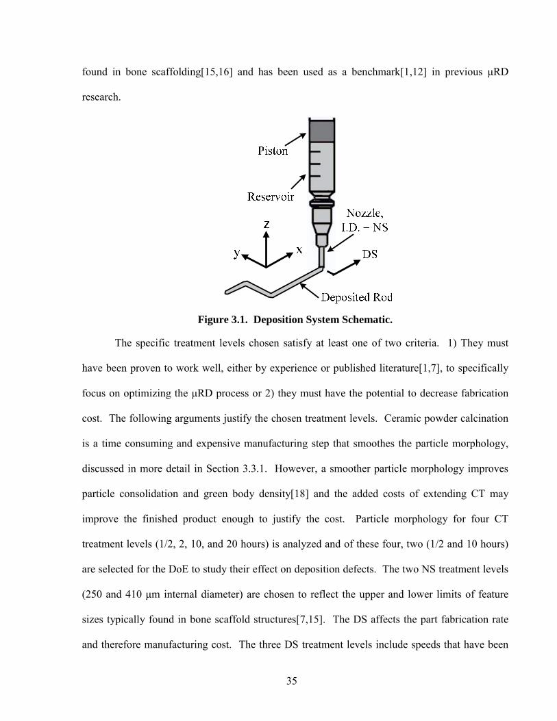
35

found in bone scaffolding[15,16] and has been used as a benchmark[1,12] in previous μRD

research.

Figure 3.1. Deposition System Schematic.

The specific treatment levels chosen satisfy at least one of two criteria. 1) They must

have been proven to work well, either by experience or published literature[1,7], to specifically

focus on optimizing the μRD process or 2) they must have the potential to decrease fabrication

cost. The following arguments justify the chosen treatment levels. Ceramic powder calcination

is a time consuming and expensive manufacturing step that smoothes the particle morphology,

discussed in more detail in Section 3.3.1. However, a smoother particle morphology improves

particle consolidation and green body density[18] and the added costs of extending CT may

improve the finished product enough to justify the cost. Particle morphology for four CT

treatment levels (1/2, 2, 10, and 20 hours) is analyzed and of these four, two (1/2 and 10 hours)

are selected for the DoE to study their effect on deposition defects. The two NS treatment levels

(250 and 410 μm internal diameter) are chosen to reflect the upper and lower limits of feature

sizes typically found in bone scaffold structures[7,15]. The DS affects the part fabrication rate

and therefore manufacturing cost. The three DS treatment levels include speeds that have been

36

commonly used in μRD bone scaffold fabrication (5 and 10 mm/s)[19] as well as one higher

speed (15 mm/s) that, if it could be used successfully, would minimize fabrication time and cost.

To analyze the effects of the treatment variables, it is important to have quantitative

metrics for evaluation. Here we define and quantify structural quality using the five weighted

cost functions, or dependent variables, that are described in depth in Section 3.2. A multivariate

analysis of variance (ANOVA) and three complementary statistical tests are used to evaluate

which treatments significantly affect the dependent variables. The DoE presented provides

statistical correlations between μRD process inputs (i.e. treatment variables), and outputs (i.e.

dependent variables). From these correlations, inferences on the mechanisms governing

deposition are made.

The following outlines the content of the paper. Section 3.2 provides details on the

materials and instruments used, the DoE setup, deposition procedure, defect quantification

method, and statistical analysis. Section 3.3 presents material processing, lattice deposition, and

statistical results. Section 3.4 discusses the experimental results, analyzing the correlations

between manufacturing treatments and part quality and postulating possible mechanisms that

govern the process. Section 3.5 includes a short experiment summary and concludes with

resulting insight gained.

3.2 Materials and Methods

3.2.1 Powder Processing and Characterization

Hydroxyapatite (HA) powder (Riedel-de Haen lot 50270) was used as the structural

material. To smoothen the surface morphology, HA powder was calcined in batches (Electric

furnace, Paragon Industries TNFQ11A) at 1100 ºC for 1/2, 2, 10, or 20 hours and furnace cooled

37

to room temperature. Calcined powder was subsequently ball milled in ethanol with cylindrical

alumina media (Ø9 mm x 14 mm) for 13 hours. The morphology of the as-received, calcined,

and calcined and ball milled powders were characterized by measuring the material density

(Pycnometer, Micromeritics 1330), specific surface area (SSA) (Nitrogen BET, Micromeritics

ASAP 2400), median particle diameter (Photo Sedimentation, Horiba CAPA-700), and imaging

by scanning electron microscopy (SEM) (Philips XL30 ESEM-FEG). X-Ray Diffraction (XRD)

(Rigaku D-Max) coupled with XRD analysis software (Jade 8.2, Materials Data Inc.) was used to

verify phases present in all the powders. Operating parameters for all instruments used can be

found in Table A.1 of Appendix A.

The 1/2 hour and 10 hour CT levels were chosen for use in the DoE in order to

investigate two particle morphologies; rough and smooth. The corresponding inks were

fabricated using a modified version of the fabrication method developed by previous

researchers[7]. The complete fabrication procedure can be found in Appendix B. Colloidal inks

are sensitive to small changes in fabrication parameters, therefore the two inks were fabricated in

parallel, solids loadings were matched, rheological modifiers were added at the same

concentration, and the pH was adjusted until the difference in final pH was 0.02. Rheological

analysis was performed using a rheometer (Bohlin CS50) with a cup and bob setup operating in

controlled shear mode with the range in shear rates spanning those in μRD[20].

The two inks were both characteristic of a yield-pseudoplastic fluid. Yield-pseudoplastic

fluids have a non-zero yield stress, meaning they are semisolid before yielding, and are shear-

thinning after yielding[21]. Rheometer data was fit to a power law model, equation (3.1), in

order to calculate nozzle pressures experienced during deposition[21]:

1nmμ γ −= (3.1)

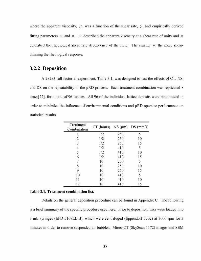
38

where the apparent viscosity, μ , was a function of the shear rate, γ , and empirically derived

fitting parameters m and n . m described the apparent viscosity at a shear rate of unity and n

described the rheological shear rate dependence of the fluid. The smaller n , the more shear-

thinning the rheological response.

3.2.2 Deposition

A 2x2x3 full factorial experiment, Table 3.1, was designed to test the effects of CT, NS,

and DS on the repeatability of the μRD process. Each treatment combination was replicated 8

times[22], for a total of 96 lattices. All 96 of the individual lattice deposits were randomized in

order to minimize the influence of environmental conditions and μRD operator performance on

statistical results.

Treatment Combination CT (hours) NS (μm) DS (mm/s)

1 1/2 250 5 2 1/2 250 10 3 1/2 250 15 4 1/2 410 5 5 1/2 410 10 6 1/2 410 15 7 10 250 5 8 10 250 10 9 10 250 15 10 10 410 5 11 10 410 10 12 10 410 15

Table 3.1. Treatment combination list.

Details on the general deposition procedure can be found in Appendix C. The following

is a brief summary of the specific procedure used here. Prior to deposition, inks were loaded into

3 mL syringes (EFD 5109LL-B), which were centrifuged (Eppendorf 5702) at 3000 rpm for 3

minutes in order to remove suspended air bubbles. Micro-CT (SkyScan 1172) images and SEM

39

micrographs of centrifuged inks displayed no evidence of a density gradient formed by the

centrifugal bubble removal process, see Section 2.3. The syringes were then fitted with a 250 or

410 μm nozzle (EFD 5125-0.25-B or 5122-0.25-B) to direct ink flow and a piston (EFD

5109PDP-B) to apply the deposition pressure. Syringes were loaded into a computer controlled

XYZ robot[23] fitted with a positive displacement micro-extrusion system, see Section 2.2.

Each of the 10 layers of the lattice contained 27 parallel rods with a center-to-center distance of

772 μm. The rod orientation of each layer was orthogonal to the previous. The first layer was

deposited 0.80 of the NS above the substrate and each subsequent layer was translated upwards

by 0.77·NS. The heights were empirically chosen to provide good lattice uniformity, based off

operator experience. The entire lattice was deposited while submerged in a non-wetting oil in

order to prevent non-uniform drying. Ink was extruded at a volumetric flowrate of

2 / 4Q NS DSπ= , where DS was either 5, 10, or 15 mm/s. Deposition was continuous, so that

each lattice was actually a long rod of ink folded upon itself to form a three-dimensional

structure. An image was captured (Hitachi KP-M22N) of each layer for future defect

quantification. After deposition, the lattices were dried in air and then removed from the

deposition substrate. After a multi-step binder burnout process, lattices were sintered at 1300 °C

for 2 hours, see Table B.1 in Appendix B.

3.2.3 Defect Quantification

This thesis presents a new defect quantification method that statistically analyzes the

effects of the deposition treatments under consideration. The quantification method was based

on a simple idea; each lattice is actually one continuous rod of ink and therefore a simple

percentage of defective length per total length can be calculated and used as the quality metric.

Recognizing that not all defects detract from part quality equally and therefore should not be

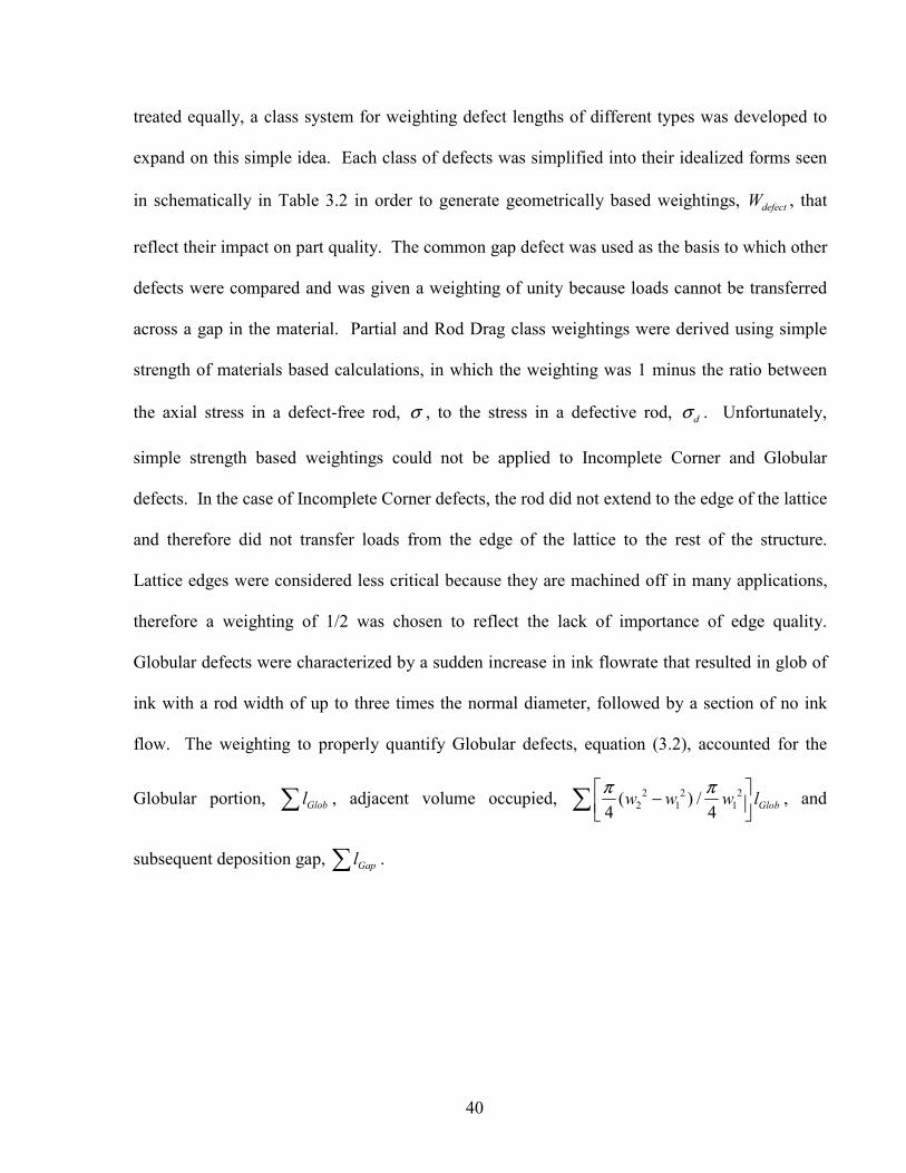
40

treated equally, a class system for weighting defect lengths of different types was developed to

expand on this simple idea. Each class of defects was simplified into their idealized forms seen

in schematically in Table 3.2 in order to generate geometrically based weightings, defectW , that

reflect their impact on part quality. The common gap defect was used as the basis to which other

defects were compared and was given a weighting of unity because loads cannot be transferred

across a gap in the material. Partial and Rod Drag class weightings were derived using simple

strength of materials based calculations, in which the weighting was 1 minus the ratio between

the axial stress in a defect-free rod, σ , to the stress in a defective rod, dσ . Unfortunately,

simple strength based weightings could not be applied to Incomplete Corner and Globular

defects. In the case of Incomplete Corner defects, the rod did not extend to the edge of the lattice

and therefore did not transfer loads from the edge of the lattice to the rest of the structure.

Lattice edges were considered less critical because they are machined off in many applications,

therefore a weighting of 1/2 was chosen to reflect the lack of importance of edge quality.

Globular defects were characterized by a sudden increase in ink flowrate that resulted in glob of

ink with a rod width of up to three times the normal diameter, followed by a section of no ink

flow. The weighting to properly quantify Globular defects, equation (3.2), accounted for the

Globular portion, Globl∑ , adjacent volume occupied, 2 2 22 1 1( ) /

4 4 Globw w w lπ π⎡ ⎤−⎢ ⎥⎣ ⎦∑ , and

subsequent deposition gap, Gapl∑ .

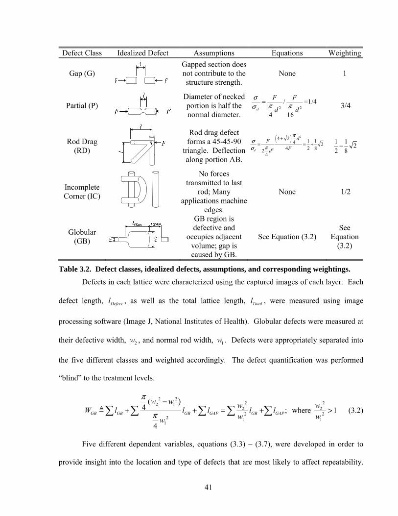
41

Defect Class Idealized Defect Assumptions Equations Weighting

Gap (G) Gapped section does

not contribute to the structure strength.

None 1

Partial (P) Diameter of necked

portion is half the normal diameter.

3/4

Rod Drag (RD)

Rod drag defect

forms a 45-45-90 triangle. Deflection along portion AB.

1 1 22 8

−

Incomplete Corner (IC)

No forces transmitted to last

rod; Many applications machine

edges.

None 1/2

Globular (GB)

GB region is defective and

occupies adjacent volume; gap is caused by GB.

See Equation (3.2) See

Equation (3.2)

Table 3.2. Defect classes, idealized defects, assumptions, and corresponding weightings. Defects in each lattice were characterized using the captured images of each layer. Each

defect length, Defectl , as well as the total lattice length, Totall , were measured using image

processing software (Image J, National Institutes of Health). Globular defects were measured at

their defective width, 2w , and normal rod width, 1w . Defects were appropriately separated into

the five different classes and weighted accordingly. The defect quantification was performed

“blind” to the treatment levels.

2 2

2 22 12 22 2

2 1 11

( )4 ; where 1

4

GB GB GB GAP GB GAP

w w w wW l l l l lw ww

π

π

−+ + = + >∑ ∑ ∑ ∑ ∑ (3.2)

Five different dependent variables, equations (3.3) – (3.7), were developed in order to

provide insight into the location and type of defects that are most likely to affect repeatability.

2 2/ =1/4

4 16d

F F

d d

σπ πσ

=

( ) 2

2

4 2 1 14 24 2 82

4d

dFFd

πσ

πσ

+= = +

42

Gap and Globular defects were specifically targeted in (3.3) and (3.4) to analyze the most

common and detrimental of defects, respectively. Most notably, defects were grouped into those

that occurred during linear sections (i.e. Steady-State defects), and those that were a result of

changes in the nozzle trajectory (i.e. Cornering defects). Included in Cornering defects were

Edge Gaps, which were Gaps resultant from edge quality deterioration at higher layers.

(%) 100%Gap Gap

Total

W lGap Defects

l×∑ (3.3)

(%) 100%GB

Total

WGlobular Defectsl

× (3.4)

- (%) 100%Gap Gap Partial Partial GB

Total

W l W l WSteady State Defects

l+ +

×∑ ∑ (3.5)

(%) 100%EdgeGap EdgeGap RD RD IC IC

Total

W l W l W lCornering Defects

l+ +

×∑ ∑ ∑ (3.6)

(%) - Total Defects Steady State Defects Cornering Defects+ (3.7)

3.2.4 Statistical Analysis

Since the treatment levels were carefully chosen, many lattices contained few defects.

Consequently there was an inordinate number of small and zero valued data values that produced

skewed dependent variable distributions and therefore the distributions were not appropriate for

ANOVA. To correct for the non-normality, transformation (3.8) was employed:

ln( 0.01)z y= + (3.8)

where y was a dependent variable and z was the new data value to be used in the statistical

analysis. The offset term, 0.01, was chosen as an arbitrarily small number that eliminated the

possibility of an undefined transformed value[24].

43

The correlations between treatments and dependent variables were categorized as either

main effects or interaction effects. Each main effect correlated the change in the dependent

variable as a result of moving one treatment from one level to another[25]. Interaction effects

correlated the change in the dependent variable when two or more treatments were varied

simultaneously[25]. Treatments that had statistically significant correlations were identified

using a multivariate ANOVA[26] with a significance value of α = 0.05. To prevent Type I

errors, an error in which the null hypothesis that a given treatment had no effects was falsely

rejected, the Bonferroni confidence interval adjustment was used[22].

Although transformation (3.8) improved the normality of dependent variable distributions

and satisfied the ANOVA assumptions, complementary statistical tests without normality

assumptions were also used to reinforce the results. Two tests were used to determine whether

the main effects of a treatment significantly affected the dependent variable distributions[22].

The Mann-Whitney test[26] tested treatments with two levels (CT and NS), whereas the Kruskal-

Wallis test[26], a generalized form of the Mann-Whitney test used in cases with more than two

levels, tested the treatment with three levels (DS). The significance value for these tests was α =

0.05.

One dependent variable data set in particular, Globular defects, contained zero valued

data points for 74 of 96 lattices. Therefore the Globular defects dependent variable most closely

resembled a Poisson distribution, which is a discrete distribution in which event occurrences are

rare[22]. The original dependent variable calculated by equation (3.4) was continuous, not

discrete, and was consequently altered to be the number of Globular defect occurrences in the

lattice instead of the weighted sum. A general loglinear analysis[26] assuming a Poisson

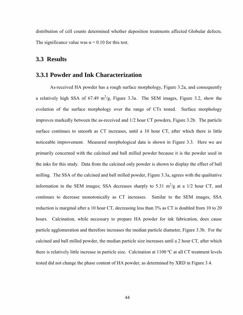
44

distribution of cell counts determined whether deposition treatments affected Globular defects.

The significance value was α = 0.10 for this test.

3.3 Results

3.3.1 Powder and Ink Characterization

As-received HA powder has a rough surface morphology, Figure 3.2a, and consequently

a relatively high SSA of 67.49 m2/g, Figure 3.3a. The SEM images, Figure 3.2, show the

evolution of the surface morphology over the range of CTs tested. Surface morphology

improves markedly between the as-received and 1/2 hour CT powders, Figure 3.2b. The particle

surface continues to smooth as CT increases, until a 10 hour CT, after which there is little

noticeable improvement. Measured morphological data is shown in Figure 3.3. Here we are

primarily concerned with the calcined and ball milled powder because it is the powder used in

the inks for this study. Data from the calcined only powder is shown to display the effect of ball

milling. The SSA of the calcined and ball milled powder, Figure 3.3a, agrees with the qualitative

information in the SEM images; SSA decreases sharply to 5.31 m2/g at a 1/2 hour CT, and

continues to decrease monotonically as CT increases. Similar to the SEM images, SSA

reduction is marginal after a 10 hour CT, decreasing less than 3% as CT is doubled from 10 to 20

hours. Calcination, while necessary to prepare HA powder for ink fabrication, does cause

particle agglomeration and therefore increases the median particle diameter, Figure 3.3b. For the

calcined and ball milled powder, the median particle size increases until a 2 hour CT, after which

there is relatively little increase in particle size. Calcination at 1100 ºC at all CT treatment levels

tested did not change the phase content of HA powder, as determined by XRD in Figure 3.4.

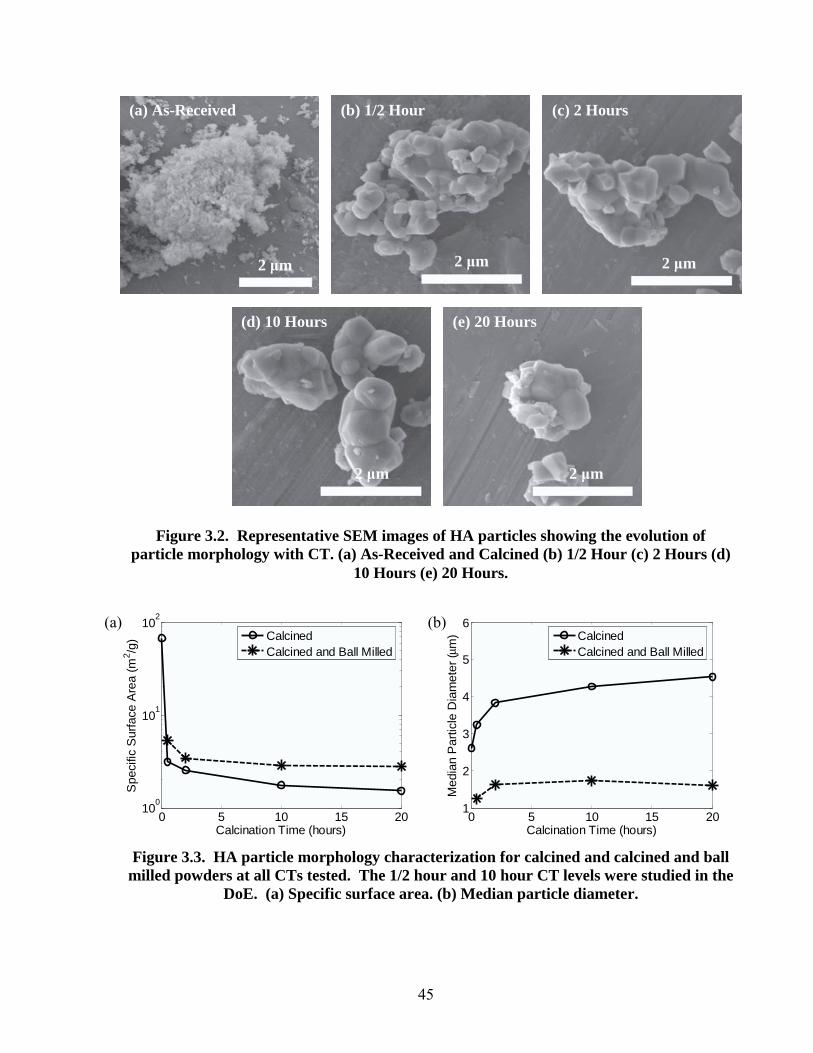
45

0 5 10 15 20100

101

102

Spe

cific

Sur

face

Are

a (m

2 /g)

Calcination Time (hours)

CalcinedCalcined and Ball Milled

0 5 10 15 201

2

3

4

5

6

Calcination Time (hours)

Med

ian

Par

ticle

Dia

met

er (μ

m) Calcined

Calcined and Ball Milled

Figure 3.3. HA particle morphology characterization for calcined and calcined and ball

milled powders at all CTs tested. The 1/2 hour and 10 hour CT levels were studied in the DoE. (a) Specific surface area. (b) Median particle diameter.

Figure 3.2. Representative SEM images of HA particles showing the evolution of particle morphology with CT. (a) As-Received and Calcined (b) 1/2 Hour (c) 2 Hours (d)

10 Hours (e) 20 Hours.

(a) As-Received (c) 2 Hours

(d) 10 Hours (e) 20 Hours

(b) 1/2 Hour

2 μm 2 μm 2 μm

2 μm 2 μm

(a) (b)

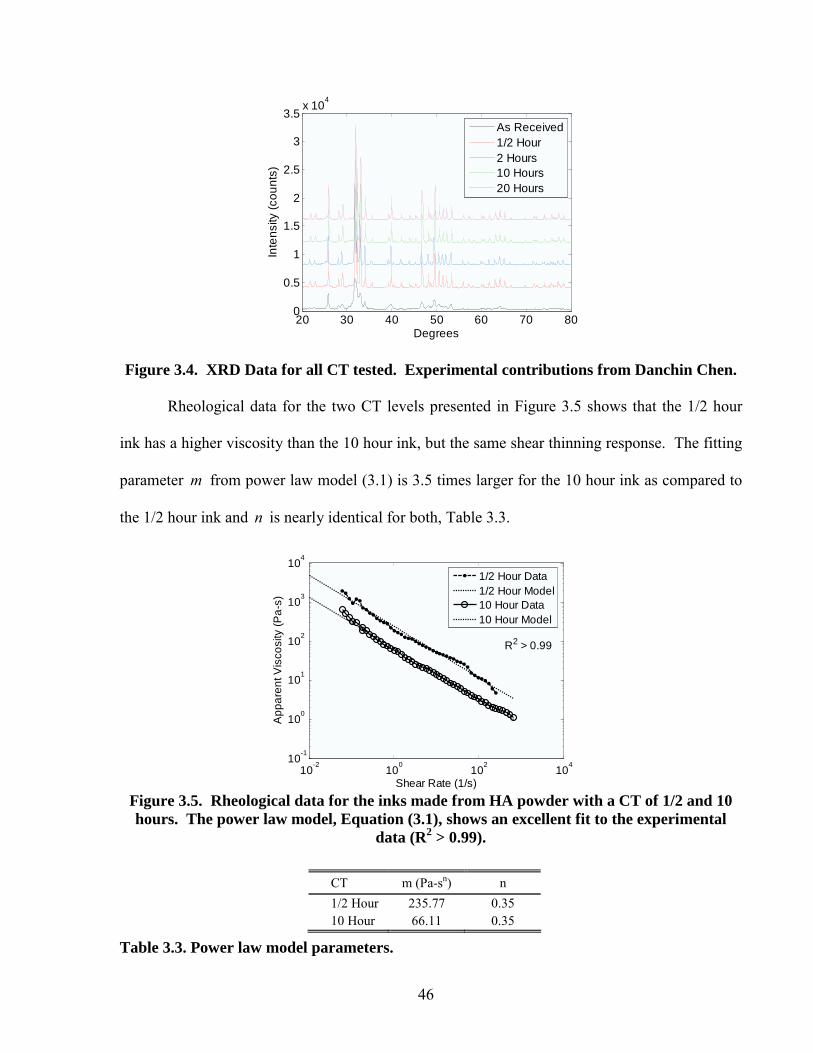
46

20 30 40 50 60 70 800

0.5

1

1.5

2

2.5

3

3.5x 104

Degrees

Inte

nsity

(cou

nts)

As Received1/2 Hour2 Hours10 Hours20 Hours

Figure 3.4. XRD Data for all CT tested. Experimental contributions from Danchin Chen.

Rheological data for the two CT levels presented in Figure 3.5 shows that the 1/2 hour

ink has a higher viscosity than the 10 hour ink, but the same shear thinning response. The fitting

parameter m from power law model (3.1) is 3.5 times larger for the 10 hour ink as compared to

the 1/2 hour ink and n is nearly identical for both, Table 3.3.

10-2 100 102 10410-1

100

101

102

103

104

Shear Rate (1/s)

App

aren

t Vis

cosi

ty (P

a-s)

1/2 Hour Data1/2 Hour Model10 Hour Data10 Hour Model

R2 > 0.99

Figure 3.5. Rheological data for the inks made from HA powder with a CT of 1/2 and 10 hours. The power law model, Equation (3.1), shows an excellent fit to the experimental

data (R2 > 0.99).

Table 3.3. Power law model parameters.

CT m (Pa-sn) n 1/2 Hour 235.77 0.35 10 Hour 66.11 0.35

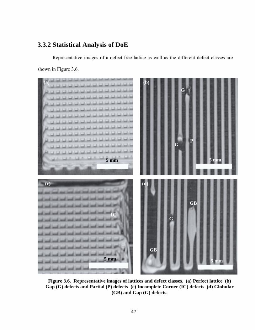
47

3.3.2 Statistical Analysis of DoE

Representative images of a defect-free lattice as well as the different defect classes are

shown in Figure 3.6.

Figure 3.6. Representative images of lattices and defect classes. (a) Perfect lattice (b) Gap (G) defects and Partial (P) defects (c) Incomplete Corner (IC) defects (d) Globular

(GB) and Gap (G) defects.

(c)

IC

(a) (b)

G P

G

GB

G

GB

(d)

5 mm 5 mm

5 mm 5 mm

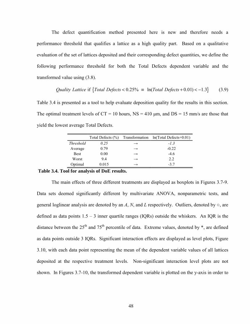
48

The defect quantification method presented here is new and therefore needs a

performance threshold that qualifies a lattice as a high quality part. Based on a qualitative

evaluation of the set of lattices deposited and their corresponding defect quantities, we define the

following performance threshold for both the Total Defects dependent variable and the

transformed value using (3.8).

if 0.25% ln( 0.01) 1.3Quality Lattice Total Defects Total Defects< ≡ + < − (3.9)

Table 3.4 is presented as a tool to help evaluate deposition quality for the results in this section.

The optimal treatment levels of CT = 10 hours, NS = 410 μm, and DS = 15 mm/s are those that

yield the lowest average Total Defects.

Total Defects (%) Transformation ln(Total Defects+0.01) Threshold 0.25 → -1.3 Average 0.79 → -0.22

Best 0.00 → -4.6 Worst 9.4 → 2.2

Optimal 0.015 → -3.7

Table 3.4. Tool for analysis of DoE results.

The main effects of three different treatments are displayed as boxplots in Figures 3.7-9.

Data sets deemed significantly different by multivariate ANOVA, nonparametric tests, and

general loglinear analysis are denoted by an A, N, and L respectively. Outliers, denoted by , are

defined as data points 1.5 – 3 inner quartile ranges (IQRs) outside the whiskers. An IQR is the

distance between the 25th and 75th percentile of data. Extreme values, denoted by *, are defined

as data points outside 3 IQRs. Significant interaction effects are displayed as level plots, Figure

3.10, with each data point representing the mean of the dependent variable values of all lattices

deposited at the respective treatment levels. Non-significant interaction level plots are not

shown. In Figures 3.7-10, the transformed dependent variable is plotted on the y-axis in order to

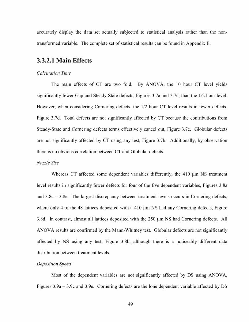
49

accurately display the data set actually subjected to statistical analysis rather than the non-

transformed variable. The complete set of statistical results can be found in Appendix E.

3.3.2.1 Main Effects

Calcination Time

The main effects of CT are two fold. By ANOVA, the 10 hour CT level yields

significantly fewer Gap and Steady-State defects, Figures 3.7a and 3.7c, than the 1/2 hour level.

However, when considering Cornering defects, the 1/2 hour CT level results in fewer defects,

Figure 3.7d. Total defects are not significantly affected by CT because the contributions from

Steady-State and Cornering defects terms effectively cancel out, Figure 3.7e. Globular defects

are not significantly affected by CT using any test, Figure 3.7b. Additionally, by observation

there is no obvious correlation between CT and Globular defects.

Nozzle Size

Whereas CT affected some dependent variables differently, the 410 μm NS treatment

level results in significantly fewer defects for four of the five dependent variables, Figures 3.8a

and 3.8c – 3.8e. The largest discrepancy between treatment levels occurs in Cornering defects,

where only 4 of the 48 lattices deposited with a 410 μm NS had any Cornering defects, Figure

3.8d. In contrast, almost all lattices deposited with the 250 μm NS had Cornering defects. All

ANOVA results are confirmed by the Mann-Whitney test. Globular defects are not significantly

affected by NS using any test, Figure 3.8b, although there is a noticeably different data

distribution between treatment levels.

Deposition Speed

Most of the dependent variables are not significantly affected by DS using ANOVA,

Figures 3.9a – 3.9c and 3.9e. Cornering defects are the lone dependent variable affected by DS

50

using the ANOVA, Figure 3.9d, where fewer defects occur at the 10 and 15 mm/s DS levels, as

compared to 5 mm/s; however there is no significant difference between the 10 and 15 mm/s

treatment levels. Similar to NS, it appears that DS changes the Globular defects data

distributions, Figure 3.9b, however there is no significant difference in DS treatment levels by

ANOVA and the Kruskal-Wallis test. Instead, the more appropriate test for Globular defects is a

general loglinear analysis assuming a Poisson distribution of cell counts, see Section 3.2.4.

There is one significant result by this test; Globular defects are fewer at the 15 mm/s DS level as

compared to the 5 mm/s level, Figure 3.9b.

3.3.2.2 Interaction Effects

A few of the main effects addressed in the previous sections are more clearly presented

by the interactions between treatments. For instance, a 10 hour CT results in more Cornering

defects, but only at the 250 μm NS level, Figure 3.10a. At a 410 μm NS for either CT, Cornering

defects are essentially non-existent, with an average of 0.001% -4.5 after transformation (3.8),

denoted by → of the lattices being Cornering defects. A similar interaction between CT and NS

is evident in Total defects, Figure 3.10b, where defects are fewer at the 410 μm level. There are

two results in which defects decrease with an increasing DS at the 410 μm NS level, but increase

at the 250 μm NS level, Figures 3.10c and 3.10d. In both cases the two NS levels perform

similarly at the 5 and 10 mm/s levels, but differently at 15 mm/s. The main effect results in

Figure 3.9d are elucidated by the interaction of NS and DS in Figure 3.10e. The 410 μm NS

level yields almost no Cornering defects, however the 250 μm NS level yields many Cornering

defects at the 5 mm/s DS level, 0.31% → -1.2. As DS is increased to 10 and 15 mm/s,

Cornering defects decrease to 0.055% → -2.7 and 0.026% → -3.3 respectively at the 250

μm NS level.

51

Calcination Time (hours)10 Hour1/2 Hour

Ln(G

ap+0

.01)

2.00

0.00

-2.00

-4.00

Calcination Time (hours)10 Hour1/2 Hour

Ln(G

lob+

0.01

)

2.00

0.00

-2.00

-4.00

Calcination Time (hours)10 Hour1/2 Hour

Ln(S

S+0.

01)

2.00

0.00

-2.00

-4.00

Calcination Time (hours)10 Hour1/2 Hour

Ln(C

orne

ring+

0.01

)

2.00

0.00

-2.00

-4.00

Calcination Time (hours)10 Hour1/2 Hour

Ln(T

otal

+0.0

1)

2.00

0.00

-2.00

-4.00

Figure 3.7. Main effects of Calcination Time (CT) on the dependent variables. (a) Gap defects (b) Globular defects (c) Steady-State defects (d) Cornering defects (e) Total defects.

Outliers denoted by , extreme values denoted by *. Brackets indicate which treatment levels are significantly different and by which tests (α = 0.05 for A and N, and α = 0.10 for

L).

(a)

(e)

(d) (c)

(b) A and N

A A

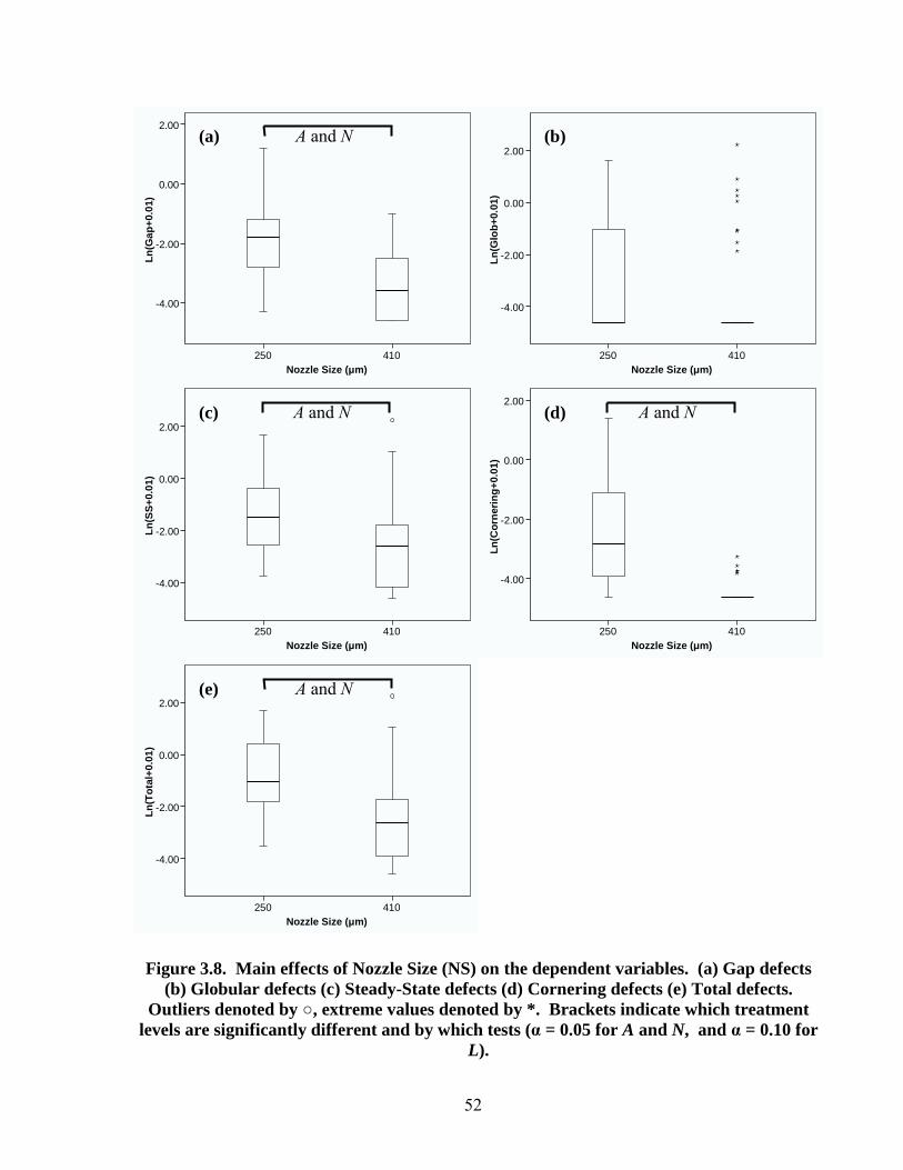
52

Nozzle Size (μm)410250

Ln(G

ap+0

.01)

2.00

0.00

-2.00

-4.00

Nozzle Size (μm)410250

Ln(G

lob+

0.01

)

2.00

0.00

-2.00

-4.00

Nozzle Size (μm)410250

Ln(S

S+0.

01)

2.00

0.00

-2.00

-4.00

Nozzle Size (μm)410250

Ln(C

orne

ring+

0.01

)

2.00

0.00

-2.00

-4.00

Nozzle Size (μm)410250

Ln(T

otal

+0.0

1)

2.00

0.00

-2.00

-4.00

Figure 3.8. Main effects of Nozzle Size (NS) on the dependent variables. (a) Gap defects (b) Globular defects (c) Steady-State defects (d) Cornering defects (e) Total defects.

Outliers denoted by , extreme values denoted by *. Brackets indicate which treatment levels are significantly different and by which tests (α = 0.05 for A and N, and α = 0.10 for

L).

A and N (a)

(e)

(d) (c)

(b)

A and N A and N

A and N

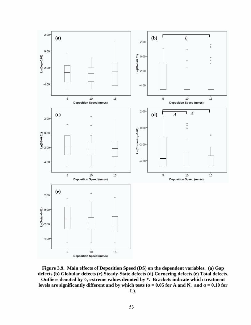
53

Deposition Speed (mm/s)15105

Ln(G

ap+0

.01)

2.00

0.00

-2.00

-4.00

Deposition Speed (mm/s)15105

Ln(G

lob+

0.01

)

2.00

0.00

-2.00

-4.00

Deposition Speed (mm/s)15105

Ln(S

S+0.

01)

2.00

0.00

-2.00

-4.00

Deposition Speed (mm/s)15105

Ln(C

orne

ring+

0.01

)

2.00

0.00

-2.00

-4.00

Deposition Speed (mm/s)15105

Ln(T

otal

+0.0

1)

2.00

0.00

-2.00

-4.00

Figure 3.9. Main effects of Deposition Speed (DS) on the dependent variables. (a) Gap defects (b) Globular defects (c) Steady-State defects (d) Cornering defects (e) Total defects.

Outliers denoted by , extreme values denoted by *. Brackets indicate which treatment levels are significantly different and by which tests (α = 0.05 for A and N, and α = 0.10 for

L).

(a)

(e)

(d) (c)

(b) L

A A

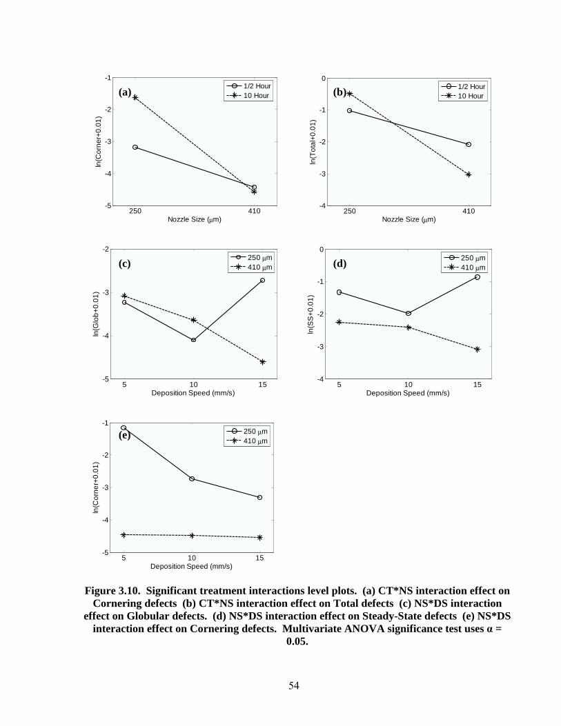
54

250 410

-5

-4

-3

-2

-1

Nozzle Size (μm)

ln(C

orne

r+0.

01)

1/2 Hour10 Hour

250 410

-4

-3

-2

-1

0

Nozzle Size (μm)

ln(T

otal

+0.0

1)

1/2 Hour10 Hour

5 10 15-5

-4

-3

-2

Deposition Speed (mm/s)

ln(G

lob+

0.01

)

250 μm410 μm

5 10 15-4

-3

-2

-1

0

Deposition Speed (mm/s)

ln(S

S+0

.01)

250 μm410 μm

5 10 15-5

-4

-3

-2

-1

Deposition Speed (mm/s)

ln(C

orne

r+0.

01)

250 μm410 μm

Figure 3.10. Significant treatment interactions level plots. (a) CT*NS interaction effect on Cornering defects (b) CT*NS interaction effect on Total defects (c) NS*DS interaction

effect on Globular defects. (d) NS*DS interaction effect on Steady-State defects (e) NS*DS interaction effect on Cornering defects. Multivariate ANOVA significance test uses α =

0.05.

(a)

(e)

(d) (c)

(b)

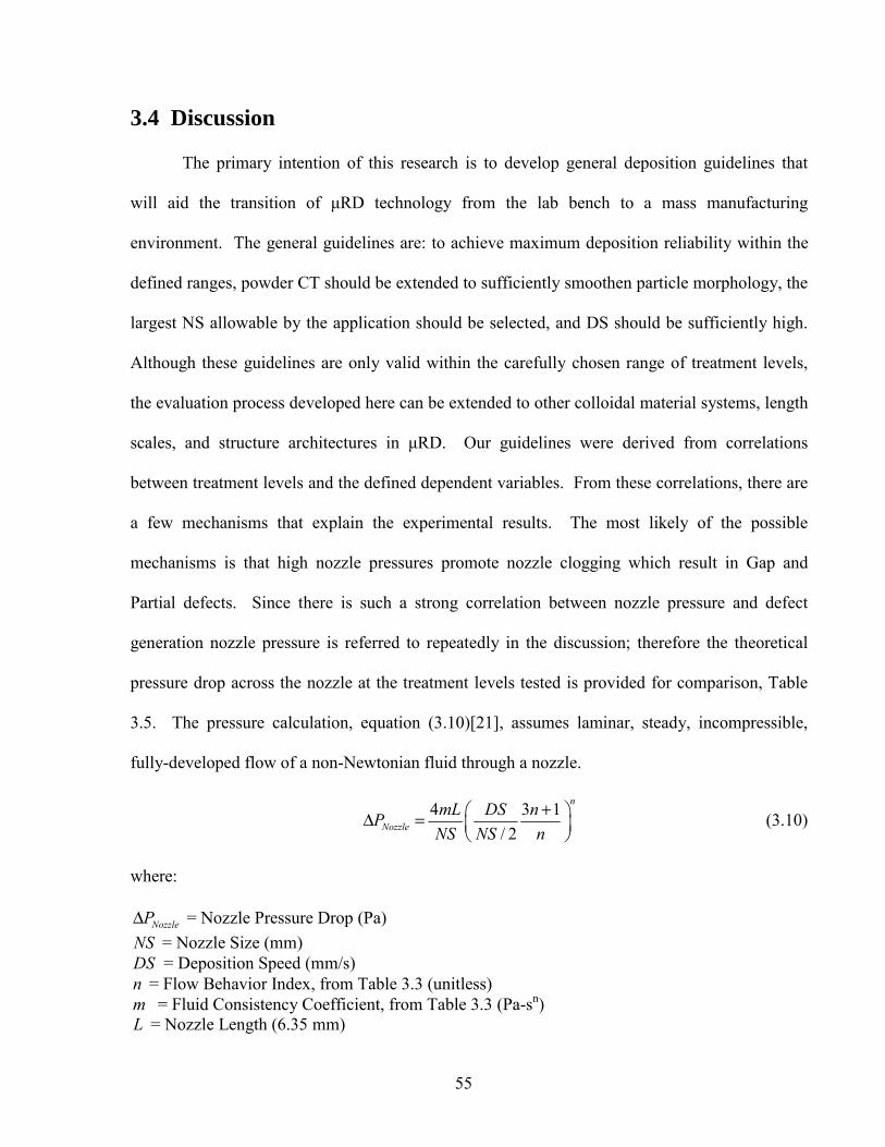
55

3.4 Discussion

The primary intention of this research is to develop general deposition guidelines that

will aid the transition of μRD technology from the lab bench to a mass manufacturing

environment. The general guidelines are: to achieve maximum deposition reliability within the

defined ranges, powder CT should be extended to sufficiently smoothen particle morphology, the

largest NS allowable by the application should be selected, and DS should be sufficiently high.

Although these guidelines are only valid within the carefully chosen range of treatment levels,

the evaluation process developed here can be extended to other colloidal material systems, length

scales, and structure architectures in μRD. Our guidelines were derived from correlations

between treatment levels and the defined dependent variables. From these correlations, there are

a few mechanisms that explain the experimental results. The most likely of the possible

mechanisms is that high nozzle pressures promote nozzle clogging which result in Gap and

Partial defects. Since there is such a strong correlation between nozzle pressure and defect

generation nozzle pressure is referred to repeatedly in the discussion; therefore the theoretical

pressure drop across the nozzle at the treatment levels tested is provided for comparison, Table

3.5. The pressure calculation, equation (3.10)[21], assumes laminar, steady, incompressible,

fully-developed flow of a non-Newtonian fluid through a nozzle.

4 3 1/ 2

n

NozzlemL DS nPNS NS n

+⎛ ⎞Δ = ⎜ ⎟⎝ ⎠

(3.10)

where:

NozzlePΔ = Nozzle Pressure Drop (Pa) NS = Nozzle Size (mm) DS = Deposition Speed (mm/s) n = Flow Behavior Index, from Table 3.3 (unitless) m = Fluid Consistency Coefficient, from Table 3.3 (Pa-sn) L = Nozzle Length (6.35 mm)

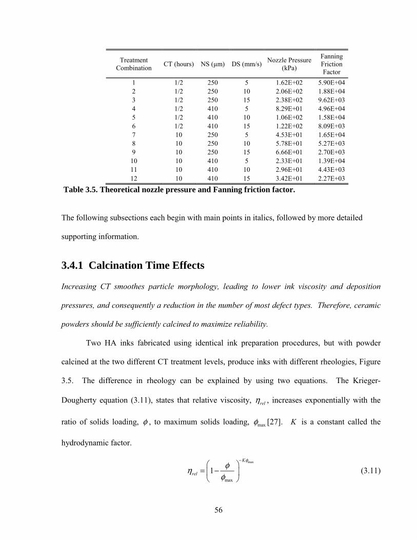
56

Treatment Combination CT (hours) NS (μm) DS (mm/s) Nozzle Pressure

(kPa)

Fanning Friction Factor

1 1/2 250 5 1.62E+02 5.90E+042 1/2 250 10 2.06E+02 1.88E+043 1/2 250 15 2.38E+02 9.62E+034 1/2 410 5 8.29E+01 4.96E+045 1/2 410 10 1.06E+02 1.58E+046 1/2 410 15 1.22E+02 8.09E+037 10 250 5 4.53E+01 1.65E+048 10 250 10 5.78E+01 5.27E+039 10 250 15 6.66E+01 2.70E+03

10 10 410 5 2.33E+01 1.39E+0411 10 410 10 2.96E+01 4.43E+0312 10 410 15 3.42E+01 2.27E+03

Table 3.5. Theoretical nozzle pressure and Fanning friction factor.

The following subsections each begin with main points in italics, followed by more detailed

supporting information.

3.4.1 Calcination Time Effects

Increasing CT smoothes particle morphology, leading to lower ink viscosity and deposition

pressures, and consequently a reduction in the number of most defect types. Therefore, ceramic

powders should be sufficiently calcined to maximize reliability.

Two HA inks fabricated using identical ink preparation procedures, but with powder

calcined at the two different CT treatment levels, produce inks with different rheologies, Figure

3.5. The difference in rheology can be explained by using two equations. The Krieger-

Dougherty equation (3.11), states that relative viscosity, relη , increases exponentially with the

ratio of solids loading, φ , to maximum solids loading, maxφ [27]. K is a constant called the

hydrodynamic factor.

max

max

1K

rel

φφη

φ

−⎛ ⎞

= −⎜ ⎟⎝ ⎠

(3.11)

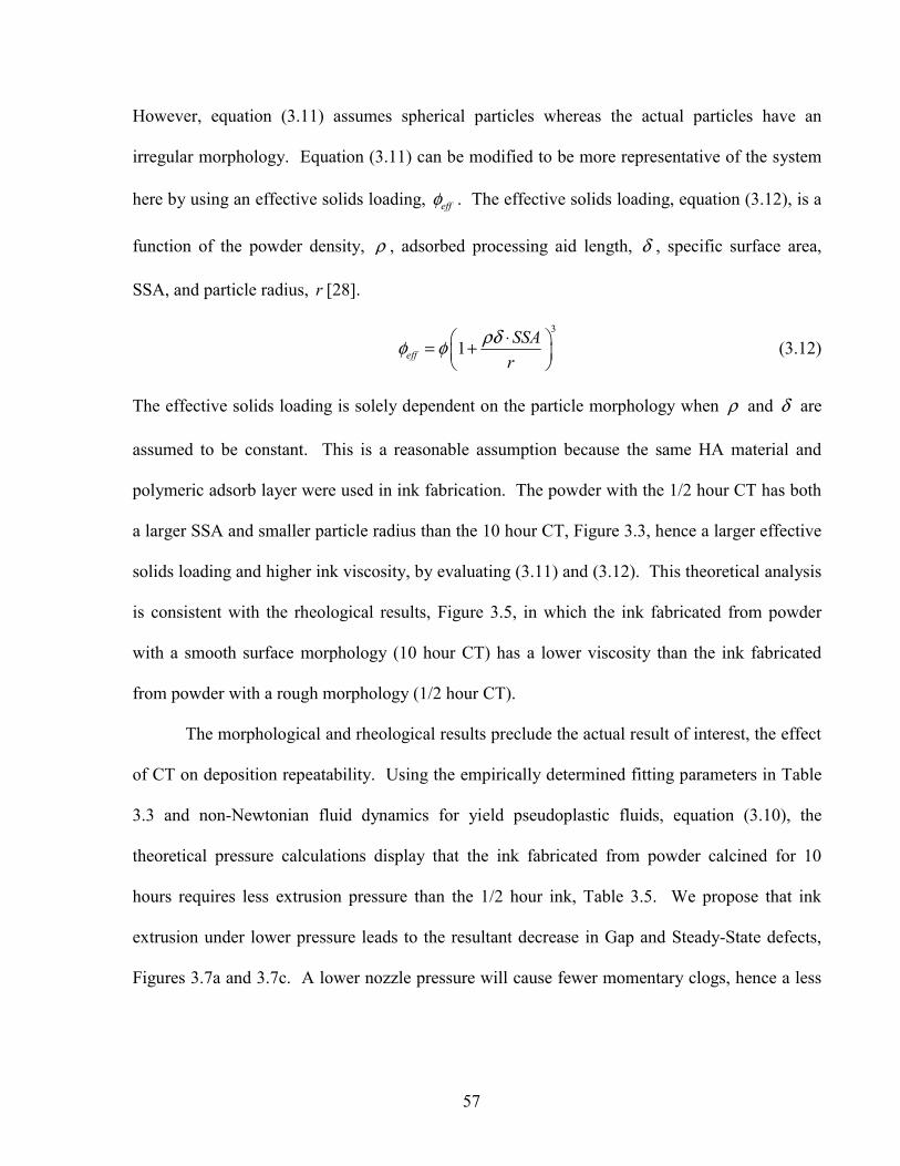
57

However, equation (3.11) assumes spherical particles whereas the actual particles have an

irregular morphology. Equation (3.11) can be modified to be more representative of the system

here by using an effective solids loading, effφ . The effective solids loading, equation (3.12), is a

function of the powder density, ρ , adsorbed processing aid length, δ , specific surface area,

SSA, and particle radius, r [28].

3

1effSSA

rρδφ φ ⋅⎛ ⎞= +⎜ ⎟

⎝ ⎠ (3.12)

The effective solids loading is solely dependent on the particle morphology when ρ and δ are

assumed to be constant. This is a reasonable assumption because the same HA material and

polymeric adsorb layer were used in ink fabrication. The powder with the 1/2 hour CT has both

a larger SSA and smaller particle radius than the 10 hour CT, Figure 3.3, hence a larger effective

solids loading and higher ink viscosity, by evaluating (3.11) and (3.12). This theoretical analysis

is consistent with the rheological results, Figure 3.5, in which the ink fabricated from powder

with a smooth surface morphology (10 hour CT) has a lower viscosity than the ink fabricated

from powder with a rough morphology (1/2 hour CT).

The morphological and rheological results preclude the actual result of interest, the effect

of CT on deposition repeatability. Using the empirically determined fitting parameters in Table

3.3 and non-Newtonian fluid dynamics for yield pseudoplastic fluids, equation (3.10), the

theoretical pressure calculations display that the ink fabricated from powder calcined for 10

hours requires less extrusion pressure than the 1/2 hour ink, Table 3.5. We propose that ink

extrusion under lower pressure leads to the resultant decrease in Gap and Steady-State defects,

Figures 3.7a and 3.7c. A lower nozzle pressure will cause fewer momentary clogs, hence a less

58

interrupted deposition. When considering the quality of internal features, CT should be extended

until particle morphology changes little with increased CT time.

The lower ink viscosity that promoted defect-free deposition in the Steady-State regime

adversely affects Cornering defects. During deposition, there is tension in the extruded rod of

ink that may misalign the structure that is being built upon if the stress exceeds the material yield

strength. Most commonly, these types of deformation defects occur at lattice corners where the

tension in the flowing ink pulls normal to the rod orientation. In this study, Cornering defects

are the most detrimental with 10 hour CT and 250 μm NS treatment levels, Figure 3.10a, because

the combination of a lower ink yield stress and more slender rods results in a more deformable

structure. Intuitively, Cornering defects are essentially non-existent at the 410 μm NS because

410 μm rods have approximately 4.5 times the theoretical bending strength[29] as compared to

250 μm rods. Although the reduced viscosity of the 10 hour CT level detracts from lattice edge

quality, the advantages of extending the CT outweigh the disadvantages. The advantages are

particularly important to the bone scaffolding application which necessitates internal uniformity

and requires post-deposition machining to shape the lattice into an anatomical geometry, which

eliminates all edge defects. Furthermore, the cornering quality can be significantly improved by

increasing the DS level, discussed in detail in Section 3.4.3, providing both internal uniformity

and precise corner deposition for applications which do have critical edge and corner

requirements. Similarly, the superiority of a longer CT has been qualitatively confirmed in

previous research studying the μRD of β–tricalcium phosphate bone scaffolds[8], a material

chemically similar to HA.

59

3.4.2 Nozzle Size Effects

A larger NS decreases deposition pressure and increases the nozzle to particle size ratio, leading

to fewer defects. Therefore the largest NS allowable by the application should be chosen.

The NS treatment has the most widespread effects of the tested treatments. Every

dependent variable except for Globular defects are significantly affected by NS; in each case the

410 μm NS level has improved deposition repeatability, Figures 3.8a and 3.8c – 3.8e. Not only

does NS largely influence nozzle pressure, Table 3.5, but the ratio of channel to particle size has

been shown to effect nozzle jamming in an environment similar to μRD[30]. By visualizing low

volume fraction suspensions flowing through arrays of single channels, Wyss et al[30] show that

the number of particles that pass through a channel before clogging increases exponentially with

the ratio of channel size to particle size and is independent of both particle flow rate and volume

fraction of solids. Wyss et al[30] attribute clogging to irreversible sticking of particles at a

channel constriction. The probability that a particle sticks to the channel wall decreases with

channel size and increases with particle size. Similar results are found in the current work,

which instead tests high volume fraction colloidal inks. At the 410 μm NS treatment, there is a

lower probability that particles will stick to the constriction at the nozzle inlet and cause clogs

(Steady-State and Gap defects). Additionally, the increased strength of the larger diameter rods

prevents material deformation during deposition, which commonly causes Cornering defects,

Figure 3.8d. Unfortunately, NS selection is typically application dependent and may be

constrained to a particular size. Given the obvious advantages of increasing the NS, the

maximum allowable NS for the application should always be selected.

60

3.4.2 Deposition Speed Effects

Increasing DS either has no effect or improves repeatability. Therefore, a high DS should be

used.

Increasing DS does not significantly detract from deposition quality. Therefore it is

advantageous to deposit the lattices at the highest speed possible. Part quality will not be

compromised and less labor and robot use time will be spent during manufacturing. Of course

there is an upper DS limit in which the fluid flow characteristics no longer permit minimal

defects and this limit must be explored. However, the fastest DS level tested in this experiment,

15 mm/s, is within the range of the popular fused deposition modeling[31,32], a rapid

prototyping technology similar to μRD. The fact that increasing DS does not adversely affect

deposition repeatability is both an interesting and unexpected result. One may anticipate that

increasing DS will compromise part quality at the benefit of manufacturing efficiency because

the required nozzle pressure is greater. However, as referenced in Section 3.4.2, previous results

have shown that the material flow rate has no bearing on material clogs, only the number of

particles passing through a channel[30]. The number of particles passing through the nozzle is

not dependent on DS and is entirely dependent on ink solids loading, which is limited to a tight

range in μRD, and the structure size.

The negative effects of an extended CT and small NS on Cornering defects, Figure 3.10a,

can be minimized by increasing the deposition speed, Figures 3.9d and 3.10e. The positive

effects of increasing deposition speed are best explained by the fluid mechanics of positive

displacement extrusion systems that extrude compressible fluids. Shown in work using the same

extrusion system as is used here[33], there exists a time lag between a change in DS and the ink

extrusion flow rate. As observed in deposition images, this lag in the ink flow rate causes a

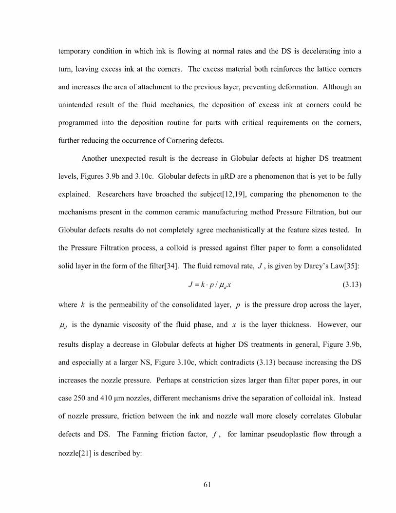
61

temporary condition in which ink is flowing at normal rates and the DS is decelerating into a

turn, leaving excess ink at the corners. The excess material both reinforces the lattice corners

and increases the area of attachment to the previous layer, preventing deformation. Although an

unintended result of the fluid mechanics, the deposition of excess ink at corners could be

programmed into the deposition routine for parts with critical requirements on the corners,

further reducing the occurrence of Cornering defects.

Another unexpected result is the decrease in Globular defects at higher DS treatment

levels, Figures 3.9b and 3.10c. Globular defects in μRD are a phenomenon that is yet to be fully

explained. Researchers have broached the subject[12,19], comparing the phenomenon to the

mechanisms present in the common ceramic manufacturing method Pressure Filtration, but our

Globular defects results do not completely agree mechanistically at the feature sizes tested. In

the Pressure Filtration process, a colloid is pressed against filter paper to form a consolidated

solid layer in the form of the filter[34]. The fluid removal rate, J , is given by Darcy’s Law[35]:

/ dJ k p xμ= ⋅ (3.13)

where k is the permeability of the consolidated layer, p is the pressure drop across the layer,

dμ is the dynamic viscosity of the fluid phase, and x is the layer thickness. However, our

results display a decrease in Globular defects at higher DS treatments in general, Figure 3.9b,

and especially at a larger NS, Figure 3.10c, which contradicts (3.13) because increasing the DS

increases the nozzle pressure. Perhaps at constriction sizes larger than filter paper pores, in our

case 250 and 410 μm nozzles, different mechanisms drive the separation of colloidal ink. Instead

of nozzle pressure, friction between the ink and nozzle wall more closely correlates Globular

defects and DS. The Fanning friction factor, f , for laminar pseudoplastic flow through a

nozzle[21] is described by:

62

2

2 8 n

f

DSf mDS NSρ

⎛ ⎞= ⎜ ⎟⎝ ⎠

(3.14)

where fρ is the fluid density and m and n are the power law fitting parameters in Table 3.3.

Assuming m and n to be constant and n less than 1 for shear-thinning fluids, the nozzle friction

is proportional to 2nDS − making the Fanning friction factors for all treatment combinations

tested decrease with an increasing DS, Table 3.5. This is in agreement with the DS main effects

for Globular defects, Figure 3.9b. Given this correlation, we conjecture that nozzle friction sheds

suspended solids from the homogenous ink, creating the separation of solid and liquid phases

realized in Globular defects. The low solid content packet first floods the structure producing the

glob of ink, followed by the high solid content packets that momentarily clog the nozzle until

building pressure expels the obtrusion; see Figure 3.6d for representative images.

The DS results suggest a potential reduction in manufacturing time as compared to

previously published deposition parameters for HA bone scaffolding lattices in which tip speeds

range from 3 mm/s[7] to 10 mm/s[19]. As a hypothetical comparison, if a manufacturing

application requires 100 lattices the size of those in this study to be fabricated, manufacturing

time could be decreased from approximately 15 to 10 hours by increasing the DS from 10 to 15

mm/s. The DS results are relevant to applications containing relatively large feature sizes;

however, we anticipate similar results at even larger feature sizes.

3.5 Summary and Conclusions

Research efforts have expanded the number of materials appropriate for μRD and have

decreased feature sizes to submicron scales[36]. However, there has been less focus on assessing

the process reliability for larger structures fabricated by μRD despite the many important

applications. This research utilized a DoE approach to determine which manufacturing

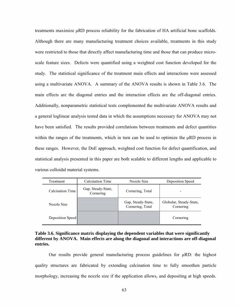
63

treatments maximize μRD process reliability for the fabrication of HA artificial bone scaffolds.

Although there are many manufacturing treatment choices available, treatments in this study

were restricted to those that directly affect manufacturing time and those that can produce micro-

scale feature sizes. Defects were quantified using a weighted cost function developed for the

study. The statistical significance of the treatment main effects and interactions were assessed

using a multivariate ANOVA. A summary of the ANOVA results is shown in Table 3.6. The

main effects are the diagonal entries and the interaction effects are the off-diagonal entries.

Additionally, nonparametric statistical tests complemented the multivariate ANOVA results and

a general loglinear analysis tested data in which the assumptions necessary for ANOVA may not

have been satisfied. The results provided correlations between treatments and defect quantities

within the ranges of the treatments, which in turn can be used to optimize the μRD process in

these ranges. However, the DoE approach, weighted cost function for defect quantification, and

statistical analysis presented in this paper are both scalable to different lengths and applicable to

various colloidal material systems.

Treatment Calcination Time Nozzle Size Deposition Speed

Calcination Time Gap, Steady-State, Cornering Cornering, Total -

Nozzle Size Gap, Steady-State, Cornering, Total

Globular, Steady-State, Cornering

Deposition Speed Cornering

Table 3.6. Significance matrix displaying the dependent variables that were significantly different by ANOVA. Main effects are along the diagonal and interactions are off-diagonal entries.

Our results provide general manufacturing process guidelines for μRD: the highest

quality structures are fabricated by extending calcination time to fully smoothen particle

morphology, increasing the nozzle size if the application allows, and depositing at high speeds.

64

The most notable result is that increasing the deposition speed does not adversely affect part

quality within the ranges tested. This result is important because manufacturing costs can be

decreased without any consequences by simply changing the deposition speed. As shown in

Table 3.6, all three treatments investigated have significant effects on the defined dependent

variables. Extending the powder calcination time smoothes particle morphology, thereby

decreasing the viscosity of the colloidal ink. The decrease in ink viscosity reduces nozzle

pressure and consequently significantly improves deposition quality of the linear sections of a

lattice. However, the less viscous, and hence less rigid, ink deforms more easily at lattice

corners, producing edge defects. Edge quality may or may not be critical depending on the

application, therefore proper calcination time is application dependent and may require a design

engineer’s judgment. Similar to many rapid prototyping technologies, decreasing feature size

increases fabrication defects. In our experiments, a smaller nozzle size required larger

deposition pressures and therefore increased the occurrence and severity of almost all types of

defects. Counterintuitively, some of the adverse effects of smaller nozzle sizes can be minimized

by increasing the deposition speed. Not only are some defects reduced, other defect quantities

remain constant and the time of manufacture can be markedly reduced by depositing at faster

rates.

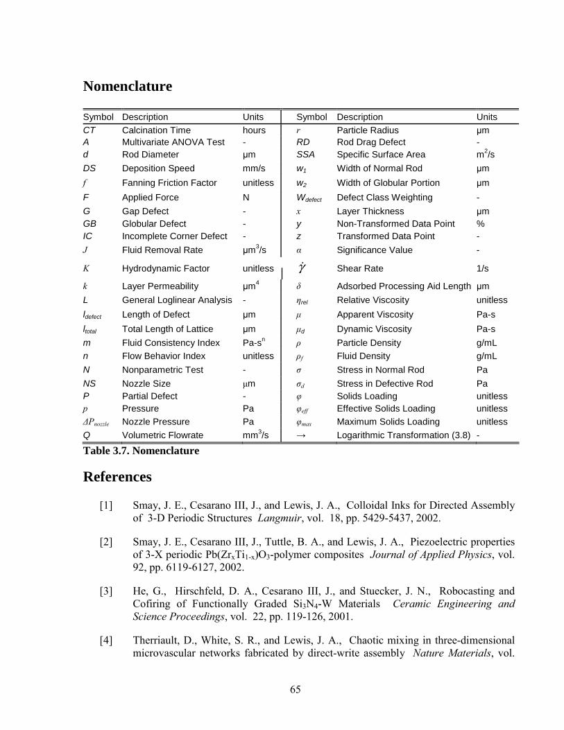
65

Nomenclature

Symbol Description Units Symbol Description Units CT Calcination Time hours r Particle Radius μm A Multivariate ANOVA Test - RD Rod Drag Defect - d Rod Diameter μm SSA Specific Surface Area m2/s DS Deposition Speed mm/s w1 Width of Normal Rod μm f Fanning Friction Factor unitless w2 Width of Globular Portion μm F Applied Force N Wdefect Defect Class Weighting - G Gap Defect - x Layer Thickness μm GB Globular Defect - y Non-Transformed Data Point % IC Incomplete Corner Defect - z Transformed Data Point - J Fluid Removal Rate μm3/s α Significance Value -

K Hydrodynamic Factor unitless

Shear Rate 1/s

k Layer Permeability μm4 δ Adsorbed Processing Aid Length μm L General Loglinear Analysis - ηrel Relative Viscosity unitless ldefect Length of Defect μm μ Apparent Viscosity Pa-s ltotal Total Length of Lattice μm μd Dynamic Viscosity Pa-s m Fluid Consistency Index Pa-sn ρ Particle Density g/mL n Flow Behavior Index unitless ρf Fluid Density g/mL N Nonparametric Test - σ Stress in Normal Rod Pa NS Nozzle Size μm σd Stress in Defective Rod Pa P Partial Defect - φ Solids Loading unitless p Pressure Pa φeff Effective Solids Loading unitless ΔPnozzle Nozzle Pressure Pa φmax Maximum Solids Loading unitless Q Volumetric Flowrate mm3/s → Logarithmic Transformation (3.8) -

Table 3.7. Nomenclature

References

[1] Smay, J. E., Cesarano III, J., and Lewis, J. A., Colloidal Inks for Directed Assembly of 3-D Periodic Structures Langmuir, vol. 18, pp. 5429-5437, 2002.

[2] Smay, J. E., Cesarano III, J., Tuttle, B. A., and Lewis, J. A., Piezoelectric properties of 3-X periodic Pb(ZrxTi1-x)O3-polymer composites Journal of Applied Physics, vol. 92, pp. 6119-6127, 2002.

[3] He, G., Hirschfeld, D. A., Cesarano III, J., and Stuecker, J. N., Robocasting and Cofiring of Functionally Graded Si3N4-W Materials Ceramic Engineering and Science Proceedings, vol. 22, pp. 119-126, 2001.

[4] Therriault, D., White, S. R., and Lewis, J. A., Chaotic mixing in three-dimensional microvascular networks fabricated by direct-write assembly Nature Materials, vol.

γ

66

2, pp. 265-271, 2003.

[5] Gratson, G. M., Xu, M., and Lewis, J. A., Direct writing of three-dimensional webs Nature, vol. 428, pp. 386, 2004.

[6] Cesarano III, J., Dellinger, J. G., Saavedra, M. P., Gill, D. D., Jamison, R. D., Grosser, B. A., Sinn-Hanlon, J. M., and Goldwasser, M. S., Customization of Load-Bearing Hydroxyapatite Lattice Scaffolds Internation Journal of Applied Ceramic Technology, vol. 2, pp. 212-220, 2005.

[7] Michna, S., Wu, W., and Lewis, J. A., Concentrated hydroxyapatite inks for direct-write assembly of 3-D periodic scaffolds Biomaterials, vol. 26, pp. 5632-5639, 2005.

[8] Miranda, P., Saiz, E., Gryn, K., and Tomsia, A. P., Sintering and Robocasting of β-Tricalcium Phosphate Scaffolds for Orthopaedic Applications Acta Biomaterialia, vol. 2, pp. 457-466, 2006.

[9] Cesarano, J., Segalman, R., and Calvert, P., Robocasting provides moldless fabrication from slurry deposition Ceramic Industry, vol. 148, pp. 94-102, Apr, 1998.

[10] Wang, J., Shaw, L. L., and Cameron, T. B., Solid Freeform Fabrication of Permanent Dental Restorations via Slurry Micro-Extrusion Journal of the American Ceramic Society, vol. 89, pp. 346-349, 2006.

[11] Stuecker, J. N., Cesarano III, J., and Hirschfeld, D. A., Control of the viscous behavior of highly concentrated mullite suspensions for robocasting Journal of Materials Processing Technology, vol. 142, pp. 318-325, 2003.

[12] Li, Q. and Lewis, J. A., Nanoparticle Inks for Directed Assembly of Three-Dimensional Periodic Structures Advanced Materials, vol. 12, pp. 1639-1643, 2003.

[13] Wang, J. and Shaw, L. L., Rheological and extrusion behavior of dental porcelain slurries for rapid prototyping applications Materials Science and Engineering A, vol. 397, pp. 314-321, 2005.

[14] Hing, K. A., Bioceramic Bone Graft Substitutes: Influence of Porosity and Chemistry International Journal of Applied Ceramic Technology, vol. 2, pp. 184-199, 2005.

[15] Chu, T.-M. G., Halloran, J. W., Hollister, S. J., and Feinberg, S. E., Hydroxyapatite Implants with Designed Internal Architecture Journal of Material Science: Materials in Medicine, vol. 12, pp. 471-478, 2001.

[16] Moroni, L., de Wijn, J. R., and van Blitterswijk, C. A., 3D Fiber-Deposited Scaffolds for Tissue Engineering: Influence of Pores Geometry and Architecture on Dynamic Mechanical Properties Biomaterials, vol. 27, pp. 974-985, 2006.

67

[17] Horng, Y. J. and Min, M. H., Effect of Calcination on Sintering of Hydroxyapatite Biomaterials, vol. 17, pp. 2059-2064, 1996.

[18] Dellinger, J. G., Development of Model Hydroxyapatite Bone Scaffolds with Multiscale Porosity for Potential Load Bearing Applications 2005. University of Illinois at Urbana-Champaign.

[19] Morissette, S. L., Lewis, J. A., Cesarano III, J., Dimos, D. B., and Baer, T., Solid Freeform Fabrication of Aqueous Alumina-Poly(vinyl alcohol) Gelcasting Suspensions Journal of the American Ceramic Society, vol. 83, pp. 2409-2416, 2000.

[20] Chhabra, R. and Richardson, J., Non-Newtonian Flow in the Process Industries, pp. 5-161, 1999. Butterworth-Heinemann. Oxford, UK. 0 5706 3770 6.

[21] Ott, R. L. and Longnecker, M., An Introduction to Statistical Methods and Data Analysis Anonymous 5, 2001. Duxbury. United States. 0-534-25122-6.

[22] Bristow, D. and Alleyne, A., "A Manufacturing System for Microscale Robotic Deposition," Proceedings of the American Controls Conference, 2003.

[23] R.G. Miller. Beyond ANOVA, Basics of Applied Statistics, New York: John Wiley & Sons, 1985.

[24] DeVor, R. E., Chang, T., and Sutherland, J. W., Statistical Quality Design and Control, Contemporary Concepts and Methods Anonymous1992. Macmillan Publishing Company. New York. 0-02-329180-X.

[25] SPSS 15.0, SPSS Inc. Chicago, IL.

[26] Krieger, I. M., Rheology of Monodisperse Latices Advances in Colloid and Interface Science, vol. 3, pp. 111-136, 1972.

[27] Lewis, J. A., Colloidal Processing of Ceramics Journal of the American Ceramic Society, vol. 83, pp. 2341-2359, 2000.

[28] J.A. Collins. Mechanical Design of Machine Elements and Machines, 2003: John Wiley & Sons, Inc., New Jersey.

[29] Wyss, H. M., Blair, D. L., Morris, J. F., Stone, H. A., and Weitz, D. A., Mechanism for clogging of microchannels Physical Review E, vol. 74, pp. 061402, 2006.

[30] Han, W., Jafari, M. A., Danforth, S. C., and Safari, A., Tool Path-Based Deposition Planning in Fused Deposition Processes Journal of Manufacturing Science and Engineering, vol. 124, pp. 462-472, 2002.

[31] Bellini, A., Güçeri, S., and Bertoldi, M., Liquefier Dynamics in Fused Deposition Journal of Manufacturing Science and Engineering, vol. 126, pp. 237-246, 2004.

68

[32] Hoelzle, D. J., Alleyne, A. G., and Wagoner Johnson, A. J., Iterative Learning Control for Robotic Deposition Using Machine Vision Submitted to ACC 2008, vol. 2008.

[33] Reed, J. S. Introduction to the Principles of Ceramic Processing, United States of America: John Wiley & Sons, Inc., 1987.

[34] Lange, F. F. and Miller, K. T., Pressure Filtration: Consolidation Kinetics and Mechanics Ceramic Bulletin, vol. 66, pp. 1498-1504, 1987.

[35] Lewis, J. A., Direct Ink Writing of 3D Functional Materials Advanced Functional Materials, vol. 16, pp. 2193-2204, 2006.

69

Chapter 4 Iterative Learning Control for Micro Robotic Deposition

4.1 Introduction

Iterative Learning Control (ILC) has been successfully applied to reference tracking

problems on a variety of different machines used in repetitive manufacturing processes[1].

However, using ILC to control an actual process, not the positioning of manufacturing toolbits,

has received less attention[2]. A potential application of ILC implemented into process control

is the modulation of build material flowrate in Micro Robotic Deposition (μRD). μRD is a Solid

Free-Form fabrication process in which a colloidal ink is extruded through a nozzle in a defined

trajectory to build three-dimensional structures[3]. The ceramic colloidal ink of interest here has

carefully tailored viscoelastic properties to facilitate ink flow through a nozzle while maintaining

a stiffness appropriate for spanning structural gaps up to 2 mm[4]. These properties allow the

fabrication of porous structures without the use of lost molds, making μRD a good fabrication

method for applications such as artificial bone scaffolds[5,6], piezoelectric actuators[7], micro-

fluidic networks[8], and photonic bandgap structures[9]. A schematic of the process and the

micro-extrusion system are shown in Figure 4.1.

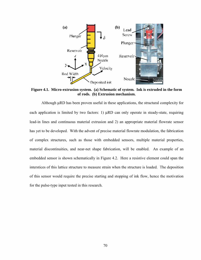
70

Figure 4.1. Micro-extrusion system. (a) Schematic of system. Ink is extruded in the form

of rods. (b) Extrusion mechanism.

Although μRD has been proven useful in these applications, the structural complexity for

each application is limited by two factors: 1) μRD can only operate in steady-state, requiring

lead-in lines and continuous material extrusion and 2) an appropriate material flowrate sensor

has yet to be developed. With the advent of precise material flowrate modulation, the fabrication

of complex structures, such as those with embedded sensors, multiple material properties,

material discontinuities, and near-net shape fabrication, will be enabled. An example of an

embedded sensor is shown schematically in Figure 4.2. Here a resistive element could span the

interstices of this lattice structure to measure strain when the structure is loaded. The deposition

of this sensor would require the precise starting and stopping of ink flow, hence the motivation

for the pulse-type input tested in this research.

(a) (b)

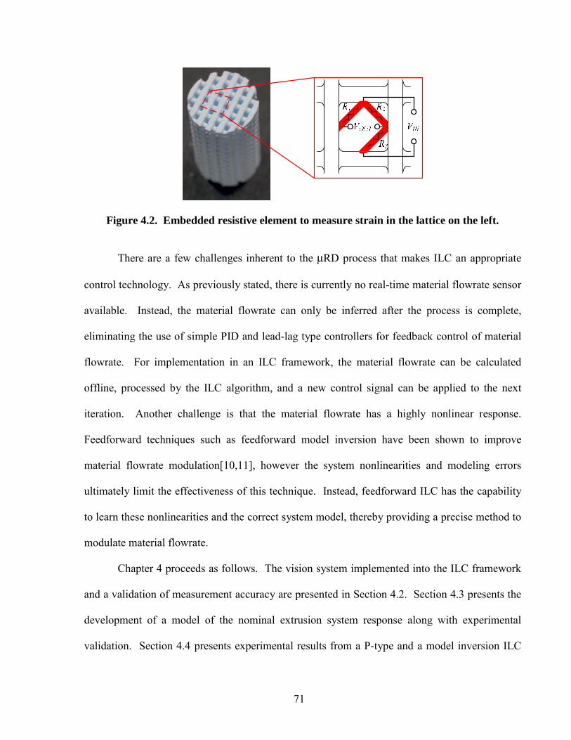
71

Figure 4.2. Embedded resistive element to measure strain in the lattice on the left.

There are a few challenges inherent to the μRD process that makes ILC an appropriate

control technology. As previously stated, there is currently no real-time material flowrate sensor

available. Instead, the material flowrate can only be inferred after the process is complete,

eliminating the use of simple PID and lead-lag type controllers for feedback control of material

flowrate. For implementation in an ILC framework, the material flowrate can be calculated

offline, processed by the ILC algorithm, and a new control signal can be applied to the next

iteration. Another challenge is that the material flowrate has a highly nonlinear response.

Feedforward techniques such as feedforward model inversion have been shown to improve

material flowrate modulation[10,11], however the system nonlinearities and modeling errors

ultimately limit the effectiveness of this technique. Instead, feedforward ILC has the capability

to learn these nonlinearities and the correct system model, thereby providing a precise method to

modulate material flowrate.

Chapter 4 proceeds as follows. The vision system implemented into the ILC framework

and a validation of measurement accuracy are presented in Section 4.2. Section 4.3 presents the

development of a model of the nominal extrusion system response along with experimental

validation. Section 4.4 presents experimental results from a P-type and a model inversion ILC

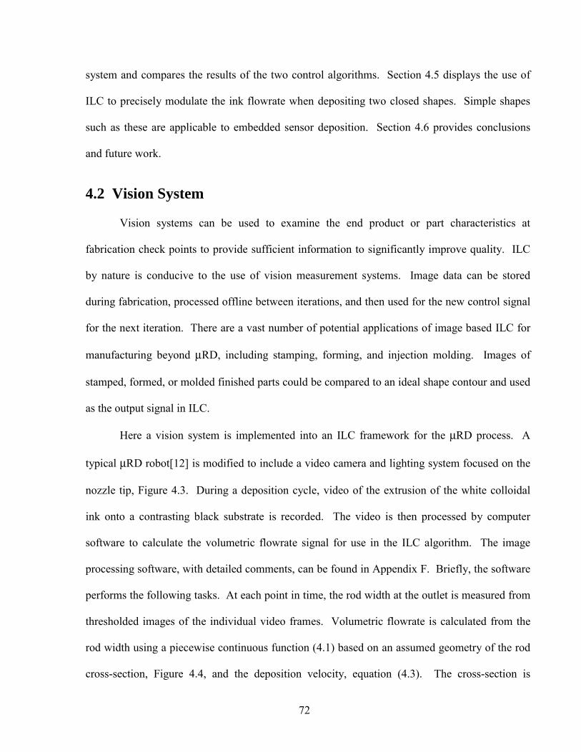
72

system and compares the results of the two control algorithms. Section 4.5 displays the use of

ILC to precisely modulate the ink flowrate when depositing two closed shapes. Simple shapes

such as these are applicable to embedded sensor deposition. Section 4.6 provides conclusions

and future work.

4.2 Vision System

Vision systems can be used to examine the end product or part characteristics at

fabrication check points to provide sufficient information to significantly improve quality. ILC

by nature is conducive to the use of vision measurement systems. Image data can be stored

during fabrication, processed offline between iterations, and then used for the new control signal

for the next iteration. There are a vast number of potential applications of image based ILC for

manufacturing beyond μRD, including stamping, forming, and injection molding. Images of

stamped, formed, or molded finished parts could be compared to an ideal shape contour and used

as the output signal in ILC.

Here a vision system is implemented into an ILC framework for the μRD process. A

typical μRD robot[12] is modified to include a video camera and lighting system focused on the

nozzle tip, Figure 4.3. During a deposition cycle, video of the extrusion of the white colloidal

ink onto a contrasting black substrate is recorded. The video is then processed by computer

software to calculate the volumetric flowrate signal for use in the ILC algorithm. The image

processing software, with detailed comments, can be found in Appendix F. Briefly, the software

performs the following tasks. At each point in time, the rod width at the outlet is measured from

thresholded images of the individual video frames. Volumetric flowrate is calculated from the

rod width using a piecewise continuous function (4.1) based on an assumed geometry of the rod

cross-section, Figure 4.4, and the deposition velocity, equation (4.3). The cross-section is

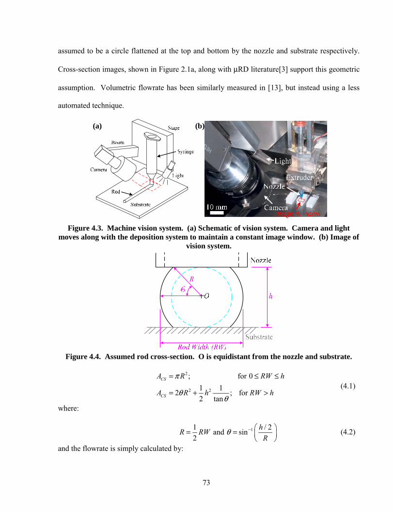
73

assumed to be a circle flattened at the top and bottom by the nozzle and substrate respectively.

Cross-section images, shown in Figure 2.1a, along with μRD literature[3] support this geometric

assumption. Volumetric flowrate has been similarly measured in [13], but instead using a less

automated technique.

Figure 4.3. Machine vision system. (a) Schematic of vision system. Camera and light

moves along with the deposition system to maintain a constant image window. (b) Image of vision system.

Figure 4.4. Assumed rod cross-section. O is equidistant from the nozzle and substrate.

2

2 2

; for 01 12 ; for 2 tan

CS

CS

A R RW h

A R h RW h

π

θθ

= ≤ ≤

= + > (4.1)

where:

11 / 2 and sin2

hR RWR

θ − ⎛ ⎞= = ⎜ ⎟⎝ ⎠

(4.2)

and the flowrate is simply calculated by:

(a) (b)

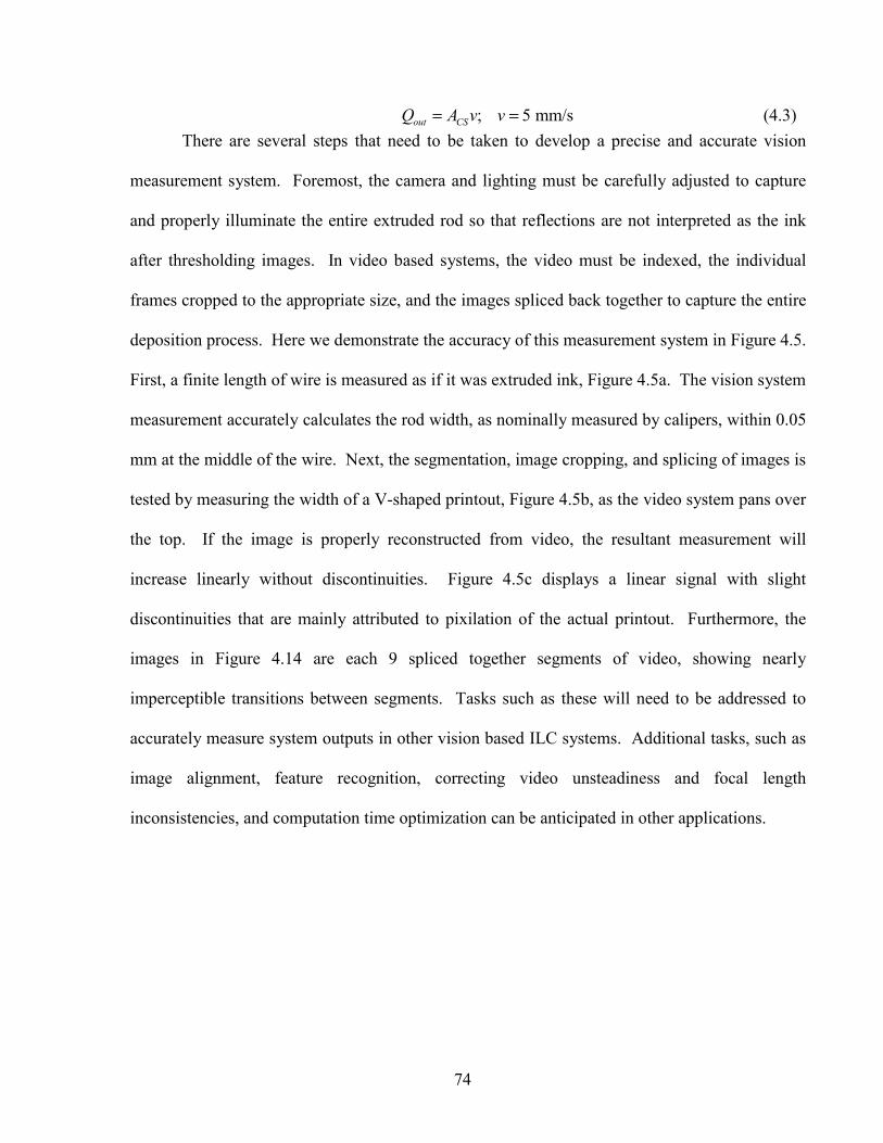
74

; 5 mm/sout CSQ A v v= = (4.3)

There are several steps that need to be taken to develop a precise and accurate vision

measurement system. Foremost, the camera and lighting must be carefully adjusted to capture

and properly illuminate the entire extruded rod so that reflections are not interpreted as the ink

after thresholding images. In video based systems, the video must be indexed, the individual

frames cropped to the appropriate size, and the images spliced back together to capture the entire

deposition process. Here we demonstrate the accuracy of this measurement system in Figure 4.5.

First, a finite length of wire is measured as if it was extruded ink, Figure 4.5a. The vision system

measurement accurately calculates the rod width, as nominally measured by calipers, within 0.05

mm at the middle of the wire. Next, the segmentation, image cropping, and splicing of images is

tested by measuring the width of a V-shaped printout, Figure 4.5b, as the video system pans over

the top. If the image is properly reconstructed from video, the resultant measurement will

increase linearly without discontinuities. Figure 4.5c displays a linear signal with slight

discontinuities that are mainly attributed to pixilation of the actual printout. Furthermore, the

images in Figure 4.14 are each 9 spliced together segments of video, showing nearly

imperceptible transitions between segments. Tasks such as these will need to be addressed to

accurately measure system outputs in other vision based ILC systems. Additional tasks, such as

image alignment, feature recognition, correcting video unsteadiness and focal length

inconsistencies, and computation time optimization can be anticipated in other applications.

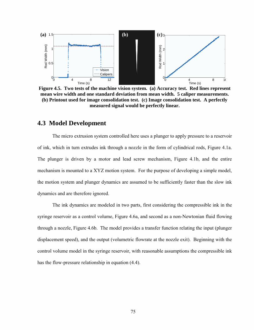
75

0 4 8 120

0.5

1

1.5

Time (s)

Rod

Wid

th (m

m)

VisionCalipers

0 4 8 10

0

1

2

3

Time (s)

Rod

Wid

th (m

m)

Figure 4.5. Two tests of the machine vision system. (a) Accuracy test. Red lines represent mean wire width and one standard deviation from mean width. 5 caliper measurements. (b) Printout used for image consolidation test. (c) Image consolidation test. A perfectly

measured signal would be perfectly linear.

4.3 Model Development

The micro extrusion system controlled here uses a plunger to apply pressure to a reservoir

of ink, which in turn extrudes ink through a nozzle in the form of cylindrical rods, Figure 4.1a.

The plunger is driven by a motor and lead screw mechanism, Figure 4.1b, and the entire

mechanism is mounted to a XYZ motion system. For the purpose of developing a simple model,

the motion system and plunger dynamics are assumed to be sufficiently faster than the slow ink

dynamics and are therefore ignored.

The ink dynamics are modeled in two parts, first considering the compressible ink in the

syringe reservoir as a control volume, Figure 4.6a, and second as a non-Newtonian fluid flowing

through a nozzle, Figure 4.6b. The model provides a transfer function relating the input (plunger

displacement speed), and the output (volumetric flowrate at the nozzle exit). Beginning with the

control volume model in the syringe reservoir, with reasonable assumptions the compressible ink

has the flow-pressure relationship in equation (4.4).

(a) (b) (c)

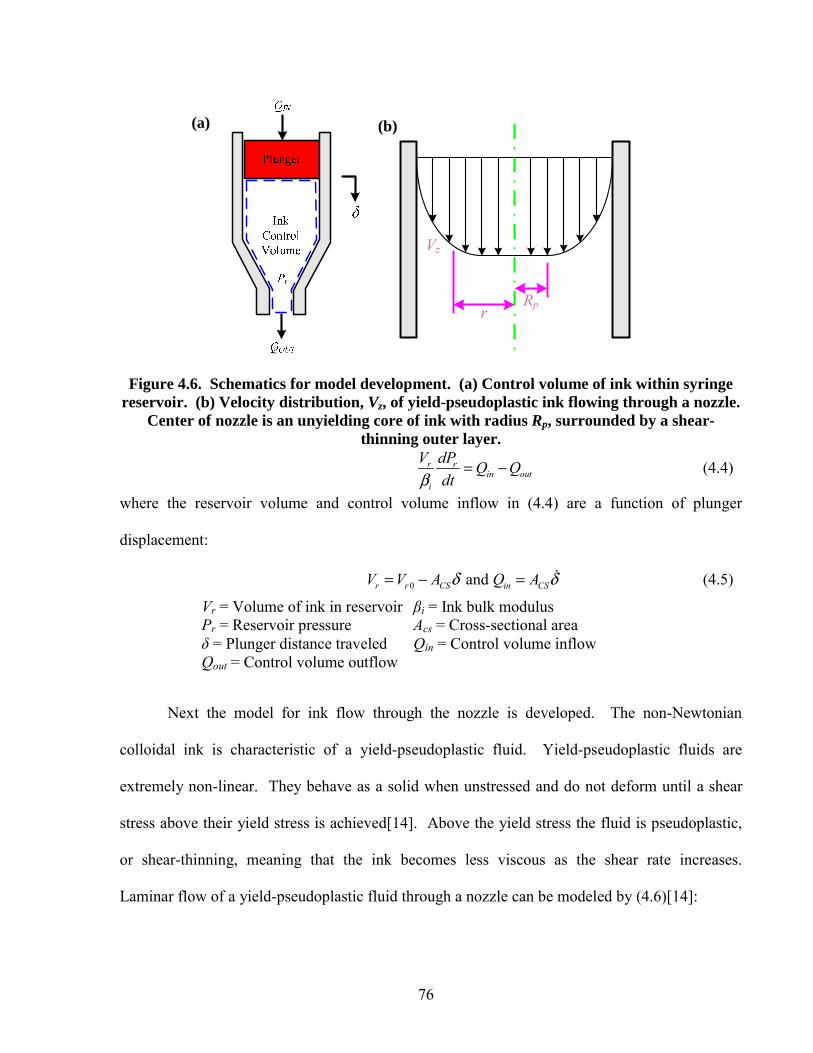
76

Rpr

Vz

Figure 4.6. Schematics for model development. (a) Control volume of ink within syringe reservoir. (b) Velocity distribution, Vz, of yield-pseudoplastic ink flowing through a nozzle.

Center of nozzle is an unyielding core of ink with radius Rp, surrounded by a shear-thinning outer layer.

r rin out

i

V dP Q Qdtβ

= − (4.4)

where the reservoir volume and control volume inflow in (4.4) are a function of plunger

displacement:

0 and r r CS in CSV V A Q Aδ δ= − = (4.5)

Next the model for ink flow through the nozzle is developed. The non-Newtonian

colloidal ink is characteristic of a yield-pseudoplastic fluid. Yield-pseudoplastic fluids are

extremely non-linear. They behave as a solid when unstressed and do not deform until a shear

stress above their yield stress is achieved[14]. Above the yield stress the fluid is pseudoplastic,

or shear-thinning, meaning that the ink becomes less viscous as the shear rate increases.

Laminar flow of a yield-pseudoplastic fluid through a nozzle can be modeled by (4.6)[14]:

Vr = Volume of ink in reservoir βi = Ink bulk modulus Pr = Reservoir pressure Acs = Cross-sectional area δ = Plunger distance traveled Qin = Control volume inflow Qout = Control volume outflow

(a) (b)

77

( )( ) ( ) ( )21/ 2

1 /3 1 2 11 for 1

3 1 2 1 1

0 for 1

nn nw

out

out

Q R nm n n n

Q

φ φ φτ φπ φ φ

φ

+ ⎧ ⎫− −− ⎪ ⎪⎛ ⎞= − + + ≤⎨ ⎬⎜ ⎟ + + +⎝ ⎠ ⎪ ⎪⎩ ⎭= >

(4.6)

where:

and 2

y rw

w

P RL

τφ τ

τ⎛ ⎞= = −⎜ ⎟⎝ ⎠

(4.7)

with the following parameters.

R = Nozzle radius L = Nozzle length n = Flow behavior index m = Fluid consistency coefficient τw = Nozzle wall shear stress τy = Ink yield stress

m and n are empirically derived parameters which describe the ink characteristics and can vary

significantly between different ink materials and even between batches of ink.

The nonlinear equation in (4.6) is not conducive to the development of a simple model to

be used in the proof of concept study here. If we assume the yield stress is small, therefore

assuming the fluid to be pseudoplastic instead of yield-pseudoplastic, equation (4.8) replaces

(4.6)[14]. Furthermore, some of the parameters in (4.8) are constant during a given experiment

and can be consolidated into the simpler equation (4.9), where the coefficient, C, and the

denominator, D, are the consolidated constants.

( )1/

3 1 /

3 1 2

nn nr

outPnQ R

n mLπ +⎛ ⎞⎛ ⎞= ⎜ ⎟⎜ ⎟+⎝ ⎠⎝ ⎠

(4.8)

1/n

rout

PQ CD

⎛ ⎞= ⎜ ⎟⎝ ⎠

(4.9)

Combining equations (4.4) and (4.9) gives:

1 1/n

r rout out CS

i

V PnD Q Q AC D

δβ

−⎛ ⎞ + =⎜ ⎟⎝ ⎠

(4.10)

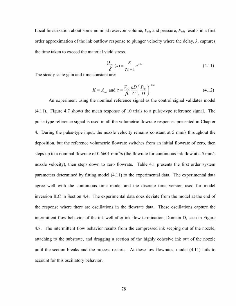
78

Local linearization about some nominal reservoir volume, Vr0, and pressure, Pr0, results in a first

order approximation of the ink outflow response to plunger velocity where the delay, λ, captures

the time taken to exceed the material yield stress.

( )1

soutQ Ks es

λ

δ τ−=

+ (4.11)

The steady-state gain and time constant are:

1 1/

0 0 and n

r rCS

i

V PnDK AC D

τβ

−⎛ ⎞= = ⎜ ⎟⎝ ⎠

(4.12)

An experiment using the nominal reference signal as the control signal validates model

(4.11). Figure 4.7 shows the mean response of 10 trials to a pulse-type reference signal. The

pulse-type reference signal is used in all the volumetric flowrate responses presented in Chapter

4. During the pulse-type input, the nozzle velocity remains constant at 5 mm/s throughout the

deposition, but the reference volumetric flowrate switches from an initial flowrate of zero, then

steps up to a nominal flowrate of 0.6601 mm3/s (the flowrate for continuous ink flow at a 5 mm/s

nozzle velocity), then steps down to zero flowrate. Table 4.1 presents the first order system

parameters determined by fitting model (4.11) to the experimental data. The experimental data

agree well with the continuous time model and the discrete time version used for model

inversion ILC in Section 4.4. The experimental data does deviate from the model at the end of

the response where there are oscillations in the flowrate data. These oscillations capture the

intermittent flow behavior of the ink well after ink flow termination, Domain D, seen in Figure

4.8. The intermittent flow behavior results from the compressed ink seeping out of the nozzle,

attaching to the substrate, and dragging a section of the highly cohesive ink out of the nozzle

until the section breaks and the process restarts. At these low flowrates, model (4.11) fails to

account for this oscillatory behavior.

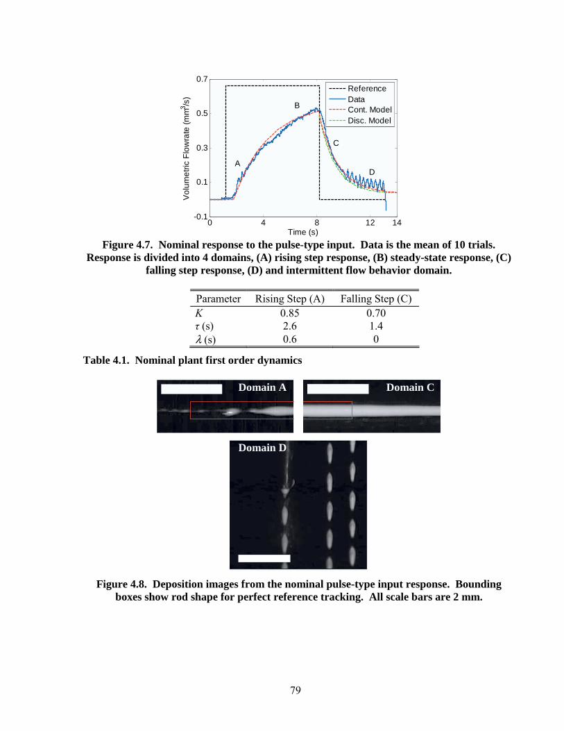
79

0 4 8 12 14-0.1

0.1

0.3

0.5

0.7

Time (s)

Vol

umet

ric F

low

rate

(mm

3 /s)

ReferenceDataCont. ModelDisc. Model

A

B

C

D

Figure 4.7. Nominal response to the pulse-type input. Data is the mean of 10 trials.

Response is divided into 4 domains, (A) rising step response, (B) steady-state response, (C) falling step response, (D) and intermittent flow behavior domain.

Parameter Rising Step (A) Falling Step (C) K 0.85 0.70 τ (s) 2.6 1.4

λ (s) 0.6 0

Table 4.1. Nominal plant first order dynamics

Figure 4.8. Deposition images from the nominal pulse-type input response. Bounding

boxes show rod shape for perfect reference tracking. All scale bars are 2 mm.

Domain A Domain C

Domain D

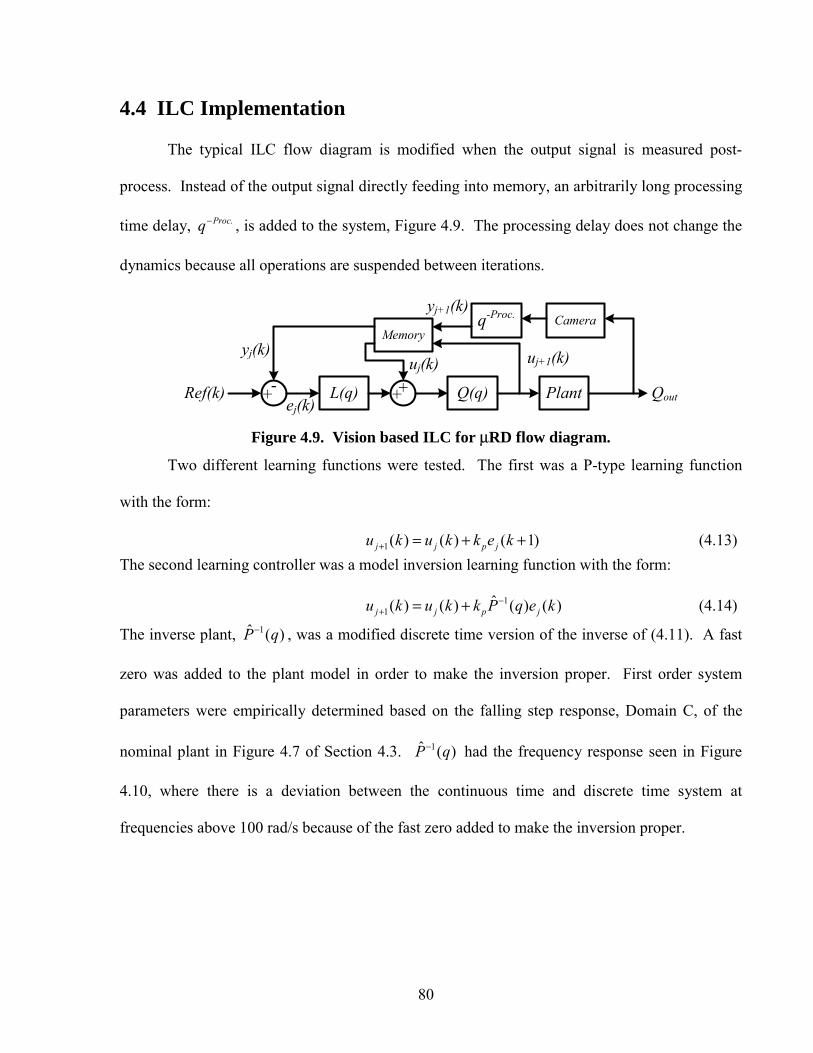
80

4.4 ILC Implementation

The typical ILC flow diagram is modified when the output signal is measured post-

process. Instead of the output signal directly feeding into memory, an arbitrarily long processing

time delay, Proc.q− , is added to the system, Figure 4.9. The processing delay does not change the

dynamics because all operations are suspended between iterations.

L(q)+- ++ Q(q) Plant

Cameraq-Proc.Memory

Ref(k)ej(k)

uj(k)yj(k) uj+1(k)

yj+1(k)

Qout

Figure 4.9. Vision based ILC for μRD flow diagram.

Two different learning functions were tested. The first was a P-type learning function

with the form:

1( ) ( ) ( 1)j j p ju k u k k e k+ = + + (4.13)

The second learning controller was a model inversion learning function with the form:

11

ˆ( ) ( ) ( ) ( )j j p ju k u k k P q e k−+ = + (4.14)

The inverse plant, 1ˆ ( )P q− , was a modified discrete time version of the inverse of (4.11). A fast

zero was added to the plant model in order to make the inversion proper. First order system

parameters were empirically determined based on the falling step response, Domain C, of the

nominal plant in Figure 4.7 of Section 4.3. 1ˆ ( )P q− had the frequency response seen in Figure

4.10, where there is a deviation between the continuous time and discrete time system at

frequencies above 100 rad/s because of the fast zero added to make the inversion proper.

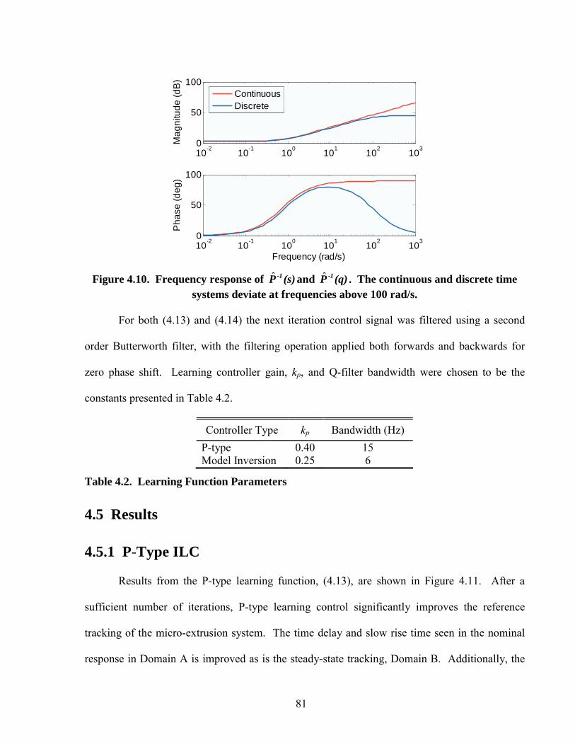
81

10-2 10-1 100 101 102 1030

50

100

Mag

nitu

de (d

B)

10-2 10-1 100 101 102 1030

50

100

Frequency (rad/s)

Pha

se (d

eg)

ContinuousDiscrete

Figure 4.10. Frequency response of ˆ -1P (s) and ˆ -1P (q) . The continuous and discrete time systems deviate at frequencies above 100 rad/s.

For both (4.13) and (4.14) the next iteration control signal was filtered using a second

order Butterworth filter, with the filtering operation applied both forwards and backwards for

zero phase shift. Learning controller gain, kp, and Q-filter bandwidth were chosen to be the

constants presented in Table 4.2.

Controller Type kp Bandwidth (Hz) P-type 0.40 15 Model Inversion 0.25 6

Table 4.2. Learning Function Parameters

4.5 Results

4.5.1 P-Type ILC

Results from the P-type learning function, (4.13), are shown in Figure 4.11. After a

sufficient number of iterations, P-type learning control significantly improves the reference

tracking of the micro-extrusion system. The time delay and slow rise time seen in the nominal

response in Domain A is improved as is the steady-state tracking, Domain B. Additionally, the

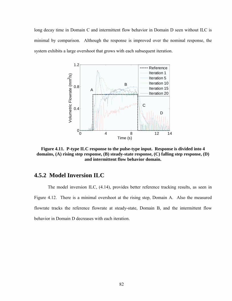
82

long decay time in Domain C and intermittent flow behavior in Domain D seen without ILC is

minimal by comparison. Although the response is improved over the nominal response, the

system exhibits a large overshoot that grows with each subsequent iteration.

0 4 8 12 140

0.4

0.8

1.2

Time (s)

Vol

umet

ric F

low

rate

(mm

3 /s)

ReferenceIteration 1Iteration 5Iteration 10Iteration 15Iteration 20

AB

C

D

Figure 4.11. P-type ILC response to the pulse-type input. Response is divided into 4 domains, (A) rising step response, (B) steady-state response, (C) falling step response, (D)

and intermittent flow behavior domain.

4.5.2 Model Inversion ILC

The model inversion ILC, (4.14), provides better reference tracking results, as seen in

Figure 4.12. There is a minimal overshoot at the rising step, Domain A. Also the measured

flowrate tracks the reference flowrate at steady-state, Domain B, and the intermittent flow

behavior in Domain D decreases with each iteration.

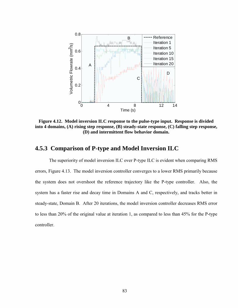
83

0 4 8 12 140

0.2

0.4

0.6

0.8

Time (s)

Vol

umet

ric F

low

rate

(mm

3 /s)

ReferenceIteration 1Iteration 5Iteration 10Iteration 15Iteration 20A

B

CD

Figure 4.12. Model inversion ILC response to the pulse-type input. Response is divided into 4 domains, (A) rising step response, (B) steady-state response, (C) falling step response,

(D) and intermittent flow behavior domain.

4.5.3 Comparison of P-type and Model Inversion ILC

The superiority of model inversion ILC over P-type ILC is evident when comparing RMS

errors, Figure 4.13. The model inversion controller converges to a lower RMS primarily because

the system does not overshoot the reference trajectory like the P-type controller. Also, the

system has a faster rise and decay time in Domains A and C, respectively, and tracks better in

steady-state, Domain B. After 20 iterations, the model inversion controller decreases RMS error

to less than 20% of the original value at iteration 1, as compared to less than 45% for the P-type

controller.

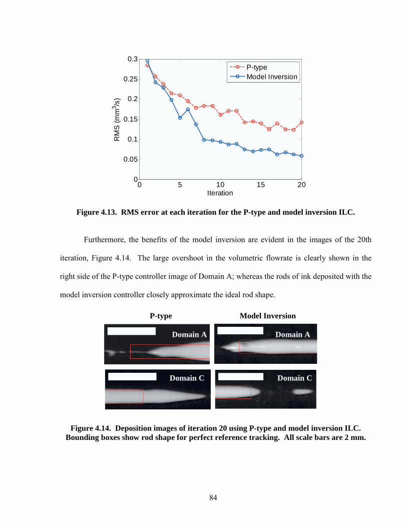
84

0 5 10 15 200

0.05

0.1

0.15

0.2

0.25

0.3

Iteration

RM

S (m

m3 /s

)

P-typeModel Inversion

Figure 4.13. RMS error at each iteration for the P-type and model inversion ILC.

Furthermore, the benefits of the model inversion are evident in the images of the 20th

iteration, Figure 4.14. The large overshoot in the volumetric flowrate is clearly shown in the

right side of the P-type controller image of Domain A; whereas the rods of ink deposited with the

model inversion controller closely approximate the ideal rod shape.

Figure 4.14. Deposition images of iteration 20 using P-type and model inversion ILC. Bounding boxes show rod shape for perfect reference tracking. All scale bars are 2 mm.

Domain A

Domain C

P-type Model Inversion

Domain A

Domain C

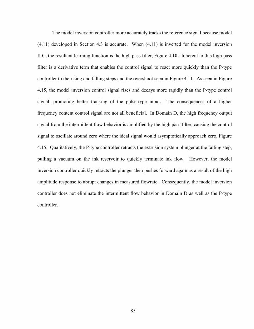
85

The model inversion controller more accurately tracks the reference signal because model

(4.11) developed in Section 4.3 is accurate. When (4.11) is inverted for the model inversion

ILC, the resultant learning function is the high pass filter, Figure 4.10. Inherent to this high pass

filter is a derivative term that enables the control signal to react more quickly than the P-type

controller to the rising and falling steps and the overshoot seen in Figure 4.11. As seen in Figure

4.15, the model inversion control signal rises and decays more rapidly than the P-type control

signal, promoting better tracking of the pulse-type input. The consequences of a higher

frequency content control signal are not all beneficial. In Domain D, the high frequency output

signal from the intermittent flow behavior is amplified by the high pass filter, causing the control

signal to oscillate around zero where the ideal signal would asymptotically approach zero, Figure

4.15. Qualitatively, the P-type controller retracts the extrusion system plunger at the falling step,

pulling a vacuum on the ink reservoir to quickly terminate ink flow. However, the model

inversion controller quickly retracts the plunger then pushes forward again as a result of the high

amplitude response to abrupt changes in measured flowrate. Consequently, the model inversion

controller does not eliminate the intermittent flow behavior in Domain D as well as the P-type

controller.

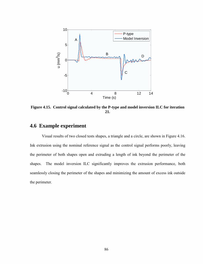
86

0 4 8 12 14-10

-5

0

5

10

Time (s)

u (m

m3 /s

)

P-typeModel InversionA

B

C

D

Figure 4.15. Control signal calculated by the P-type and model inversion ILC for iteration 21.

4.6 Example experiment

Visual results of two closed tests shapes, a triangle and a circle, are shown in Figure 4.16.

Ink extrusion using the nominal reference signal as the control signal performs poorly, leaving

the perimeter of both shapes open and extruding a length of ink beyond the perimeter of the

shapes. The model inversion ILC significantly improves the extrusion performance, both

seamlessly closing the perimeter of the shapes and minimizing the amount of excess ink outside

the perimeter.

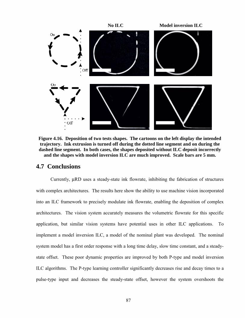
87

Figure 4.16. Deposition of two tests shapes. The cartoons on the left display the intended trajectory. Ink extrusion is turned off during the dotted line segment and on during the dashed line segment. In both cases, the shapes deposited without ILC deposit incorrectly

and the shapes with model inversion ILC are much improved. Scale bars are 5 mm.

4.7 Conclusions

Currently, μRD uses a steady-state ink flowrate, inhibiting the fabrication of structures

with complex architectures. The results here show the ability to use machine vision incorporated

into an ILC framework to precisely modulate ink flowrate, enabling the deposition of complex

architectures. The vision system accurately measures the volumetric flowrate for this specific

application, but similar vision systems have potential uses in other ILC applications. To

implement a model inversion ILC, a model of the nominal plant was developed. The nominal

system model has a first order response with a long time delay, slow time constant, and a steady-

state offset. These poor dynamic properties are improved by both P-type and model inversion

ILC algorithms. The P-type learning controller significantly decreases rise and decay times to a

pulse-type input and decreases the steady-state offset, however the system overshoots the

No ILC Model inversion ILC

88

reference trajectory. The model inversion learning controller improves on the P-type controller,

accurately tracking the reference with minimal overshoot and therefore converging to a lower

RMS error. The improvement is a result of the inherent derivative from the model inversion,

however there is a consequence to the derivative term. The derivate causes the system to react to

sharp changes in the measured flowrate during a period of intermittent ink flow, causing the

control signal to oscillate. When comparing the two controllers using the Domains given in

Figure 4.7, the model inversion ILC performs better in Domains A, B, and C whereas the P-type

ILC performs better in Domain D. This suggests that future work may include time varying

algorithms. Finally, an example relevant to the deposition of interstitial structures, such as

embedded micro-sized sensors, displays that the model inversion ILC properly extrudes the ink,

producing structures with a seamless perimeter and minimal excess material outside the

perimeter.

89

Nomenclature

Symbol Description Units C Transfer Function Coefficient unitless D Transfer Function Denominator unitless e Error Signal mm3/s h Nozzle Height μm j Iteration Index Iterations K Steady-State Gain unitless k Time Step Index Time Steps kp Proportional Gain unitless L Nozzle Length mm L(q) Learning Filter - m Fluid Consistency Index Pa-sn n Flow Behavior Index unitless Pr Reservoir Pressure Pa

Model Inverse -

Q(q) Q-Filter - Qin Volumetric Flowrate In mm3/s Qout Volumetric Flowrate Out mm3/s R Nozzle Radius μm RW Rod Width μm u Control Signal mm3/s v Nozzle Velocity mm/s Vr Reservoir Volume mm3 βi Ink Bulk Modulus Pa δ Plunger Displacement μm θ Correction Factor Angle rad λ Time Delay s τ Time Constant s τw Wall Shear Stress Pa

τy Yield Stress Pa

Table 4.3. Nomenclature

References

[1] Bristow, D.A., Tharayil, M., and Alleyne, A.G., A Survey of Iterative Learning Control, IEEE Control Systems Magazine, pp. 96-114, 2006.

[2] Lee, K.S. and Lee, J.H., Iterative Learning Control-Based Batch Process Control Technique for Integrated Control of End Product Properties and Transient Profiles of Process Variables, Journal of Process Control, vol. 13, pp. 607-621, 2003.

1ˆ ( )P− ⋅

90

[3] Cesarano, J., Segalman, R., and Calvert, P., Robocasting Provides Moldless Fabrication From Slurry Deposition, Ceramic Industry, vol. 148, no. 4, pp. 94-102, 1998.

[4] Smay, J.E., Cesarano III, J., and Lewis, J.A., Colloidal Inks for Directed Assembly of 3-D Periodic Structures, Langmuir, vol. 18, no. 14, pp. 5429-5437, 2002.

[5] Michna, S., Wu, W., and Lewis, J.A., Concentrated Hydroxyapatite Inks for Direct-Write Assembly of 3-D Periodic Scaffolds, Biomaterials, vol. 26, pp. 5632-5639, 2005.

[6] Miranda, P., Saiz, E., Gryn, K., and Tomsia, A.P., Sintering and Robocasting of β-Tricalcium Phosphate Scaffolds for Orthopaedic Applications, Acta Biomaterialia, vol. 2, pp. 457-466, 2006.

[7] Smay, J.E., Cesarano III, J., Tuttle, B.A., and Lewis, J.A., Piezoelectric Properties of 3-X Periodic Pb(ZrxTi1-x)O3-Polymer Composites, Journal of Applied Physics, vol. 92, no. 10, pp. 6119-6127, 2002.

[8] Therriault, D., White, S.R., and Lewis, J.A., Chaotic Mixing in Three-Dimensional Microvascular Networks Fabricated by Direct-Write Assembly, Nature Materials, vol. 2, pp. 265-271, 2003.

[9] Gratson, G.M., Xu, M., and Lewis, J.A., Direct Writing of Three-Dimensional Webs, Nature, vol. 428, pp. 386, 2004.

[10] Han, W. and Jafari, M.A., Coordination Control of Positioning and Deposition in Layered Manufacturing, IEEE Transactions on Industrial Electronics, vol. 54, no. 1, pp. 651-659, 2007.

[11] Bristow, D. and Alleyne, A., A Manufacturing System for Microscale Robotic Deposition, Proceedings of the American Controls Conference, pp. 2620-2625, 2003.

[12] Bellini, A., Güçeri, S., and Bertoldi, M., Liquefier Dynamics in Fused Deposition, Journal of Manufacturing Science and Engineering, vol. 126, pp. 237-246, 2004 .

[13] Chhabra, R.P., Richardson, J.F., Non-Newtonian Flow in the Process Industries. Oxford, UK: Butterworth-Heinemann, 1999.

91

Chapter 5 Summary

5.1 Summary

Micro Robotic Deposition (μRD) is a relatively new solid freeform fabrication technique

that enables the fabrication of complex ceramic structures without the use of lost molds and

lengthy binder burnout processes. To date, research efforts have primarily taken a materials

science approach to the technological development, building a library of material systems

appropriate for μRD. The research presented here has two primary directions. One of these

directions utilizes an industrial process optimization approach; the second direction involves a

dynamics and controls approach. By approaching the technology from a different area of

expertise, two interesting new dimensions have been added to μRD.

The focus of Chapter 3 is on developing general deposition guidelines to achieve the

highest possible μRD process reliability. The goal is for these guidelines to help transition μRD

from the research bench to the mass manufacturing environment. To this end, a Design of

Experiments (DoE) technique is borrowed from the industrial engineering community to

evaluate the μRD process. First reliability metrics are defined based on the type, location, and

severity of fabrication defects. With these new metrics, statistical correlations are investigated

between the three manufacturing treatments (calcination time, nozzle size, and deposition speed)

and the five defined metrics. From the correlations, mechanisms that govern the deposition

process are postulated, citing the statistical results and previous research as backing evidence.

The DoE also reveals which manufacturing treatment levels yielded the highest reliability,

providing guidelines that should hold true for future deposition.

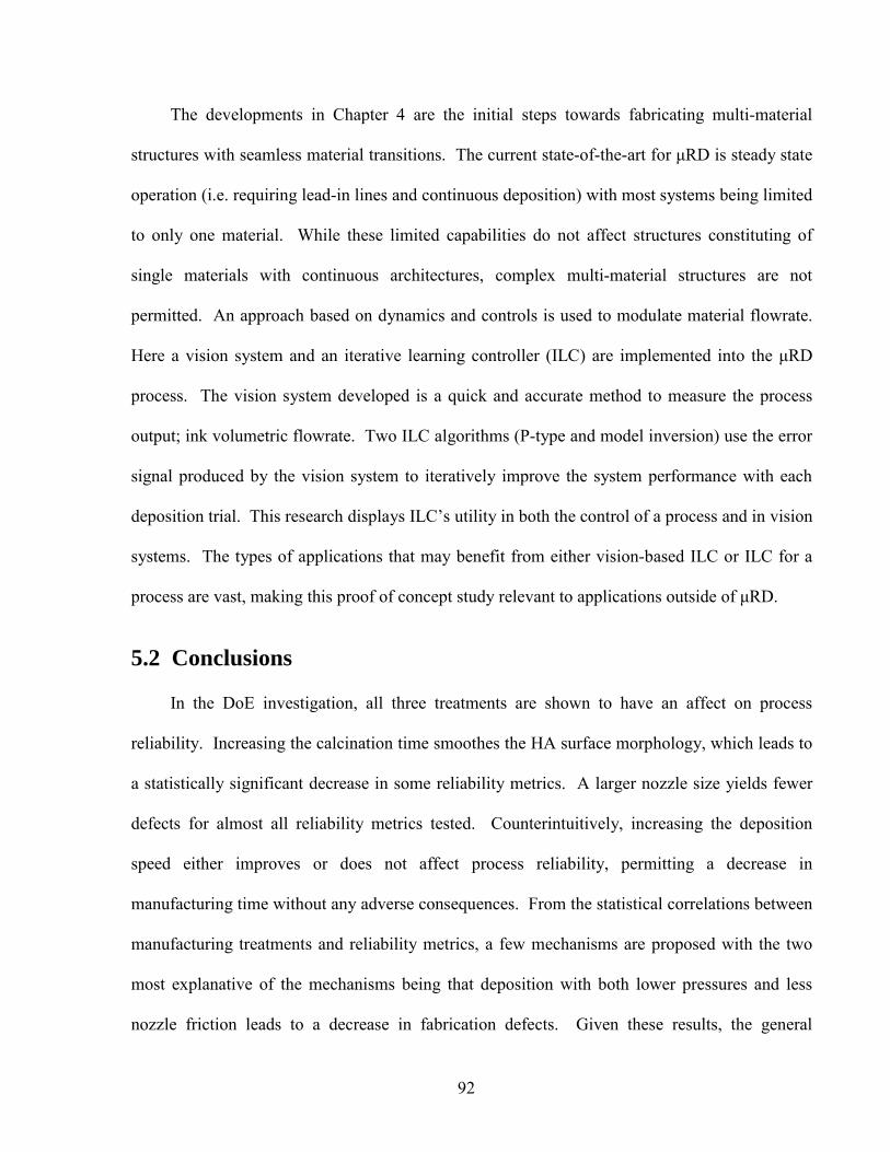
92

The developments in Chapter 4 are the initial steps towards fabricating multi-material

structures with seamless material transitions. The current state-of-the-art for μRD is steady state

operation (i.e. requiring lead-in lines and continuous deposition) with most systems being limited

to only one material. While these limited capabilities do not affect structures constituting of

single materials with continuous architectures, complex multi-material structures are not

permitted. An approach based on dynamics and controls is used to modulate material flowrate.

Here a vision system and an iterative learning controller (ILC) are implemented into the μRD

process. The vision system developed is a quick and accurate method to measure the process

output; ink volumetric flowrate. Two ILC algorithms (P-type and model inversion) use the error

signal produced by the vision system to iteratively improve the system performance with each

deposition trial. This research displays ILC’s utility in both the control of a process and in vision

systems. The types of applications that may benefit from either vision-based ILC or ILC for a

process are vast, making this proof of concept study relevant to applications outside of μRD.

5.2 Conclusions

In the DoE investigation, all three treatments are shown to have an affect on process

reliability. Increasing the calcination time smoothes the HA surface morphology, which leads to

a statistically significant decrease in some reliability metrics. A larger nozzle size yields fewer

defects for almost all reliability metrics tested. Counterintuitively, increasing the deposition

speed either improves or does not affect process reliability, permitting a decrease in

manufacturing time without any adverse consequences. From the statistical correlations between

manufacturing treatments and reliability metrics, a few mechanisms are proposed with the two

most explanative of the mechanisms being that deposition with both lower pressures and less

nozzle friction leads to a decrease in fabrication defects. Given these results, the general

93

deposition guidelines are: calcination time should be lengthened to a point where the

morphological improvements are marginal, the largest nozzle size allowable by the application

should always be selected, and the deposition speed should be sufficiently fast.

Results from the ILC investigation show that the nominal system performance is poor,

having a first order response with a large time constant and a long time delay. The two different

ILC algorithms (P-type and model inversion) improve on the nominal system response,

decreasing the RMS error to less than half the nominal system after a number of iterations. The

model inversion algorithm performs more than twice as well as the P-type algorithm because the

model inversion algorithm has a larger response to higher frequency content in the error signal.

Interestingly, the model inversion algorithm does not perform as well as the P-type algorithm in

all domains of the system response, suggesting that a time varying algorithm may further

improve system performance. In an example of deposition performance, the model inversion

ILC also performs better than the nominal system when fabricating simple shapes.

5.3 Important Contributions

Previous μRD research has infrequently addressed process reliability, only performing ad

hoc adjustments to the manufacturing treatments. The work in Chapter 3 is the first to take a

scientific approach to the treatment optimization. Also new defect quantification metrics are

developed, providing the μRD community with a quality evaluation system that can be used in

future work and modified if need be. Chapter 4 is a proof of concept study and is a new

extension of ILC in two respects. It is the first to our knowledge to apply ILC to a mechanical

process and one of the first to apply ILC to any process. Also, to our knowledge it is the first to

incorporate machine vision as a sensing mechanism in the ILC framework.

94

5.4 Future Work

Multi-material deposition has the potential to be an important extension of the base μRD

technology. Possible applications include near-net shape fabrication, structures with multiple

domains of different material properties, and the integration of sensors and actuators within

larger structures. Near-net shape fabrication is particularly important to the bone scaffold

application because scaffolds could be fabricated in the shape of anatomical defects, eliminating

a time consuming and costly machining process. To this end, the ILC algorithms used in

Chapter 4 on a single material system will be fine tuned and then implemented on a more

complex multi-material extrusion system. The ILC algorithm will be incorporated with new

material transition algorithms to enable the fabrication of structures with seamless material

transitions. At first, simple near-net shapes will be fabricated, followed by more complex shapes

with irregular contours and frequent material transitions.

95

Appendix A Materials and Instruments

A.1 Materials

A.1.1 Hydroxyapatite

Riedel-de Haen (Sigma-Aldrich 04238)

Ca5(OH)(PO4)3. Calcium phosphate materials have received much attention as possible

bone replacement materials because of their osteoconductive capabilities[1]. One of the calcium

phosphate materials, hydroxyapatite, has been a popular choice of materials because it is

chemically similar to the mineral component of natural bone[2]. For the research presented here,

HA powder was used as the solid phase of the colloidal inks. The purchased powder has a rough

surface morphology, Figure A.1, which is not ideal for colloidal stabilization. The surface

morphology is easily modified by a heat treatment process called calcination. The effects of

calcination are presented in detail in Chapter 3.

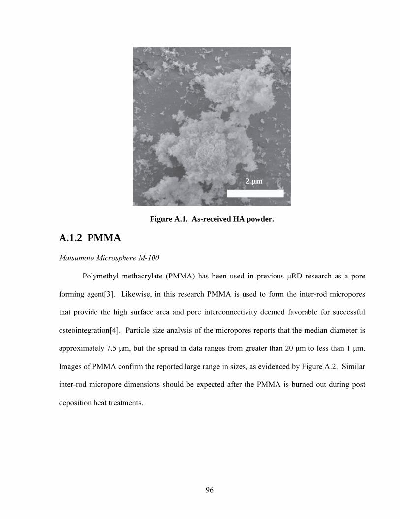
96

Figure A.1. As-received HA powder.

A.1.2 PMMA

Matsumoto Microsphere M-100

Polymethyl methacrylate (PMMA) has been used in previous μRD research as a pore

forming agent[3]. Likewise, in this research PMMA is used to form the inter-rod micropores

that provide the high surface area and pore interconnectivity deemed favorable for successful

osteointegration[4]. Particle size analysis of the micropores reports that the median diameter is

approximately 7.5 μm, but the spread in data ranges from greater than 20 μm to less than 1 μm.

Images of PMMA confirm the reported large range in sizes, as evidenced by Figure A.2. Similar

inter-rod micropore dimensions should be expected after the PMMA is burned out during post

deposition heat treatments.

2 μm

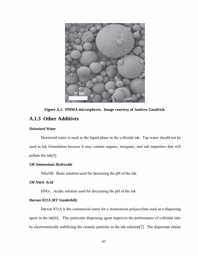
97

Figure A.2. PMMA microspheres. Image courtesy of Andrew Goodrich.

A.1.3 Other Additives

Deionized Water

Deionized water is used as the liquid phase in the colloidal ink. Tap water should not be

used in ink formulation because it may contain organic, inorganic, and salt impurities that will

pollute the ink[5].

5M Ammonium Hydroxide

NH4OH. Basic solution used for increasing the pH of the ink.

1M Nitric Acid

HNO3. Acidic solution used for decreasing the pH of the ink.

Darvan 821A (RT Vanderbilt)

Darvan 821A is the commercial name for a Ammonium polyacrylate used as a dispersing

agent in the ink[6]. This particular dispersing agent improves the performance of colloidal inks

by electrosterically stabilizing the ceramic particles in the ink solution[7]. The dispersant chains

10 μm

98

provide a high charge density on the particle surfaces, creating large repulsive forces that prevent

particle agglomeration.

Methocel (Dow Chemical)

Methocel is a cellulose binder[8] that provides the ink with the proper viscoelastic

properties for μRD. For this formulation, the Methocel binder is added in low concentrations so

that post-deposition binder burnout processes proceed more quickly than the lengthy burnout

process required for high binder concentration ceramics[9].

1-Octanol (Fisher Scientific)

1-Octanol is commercial antifoaming agent.

Polyethylenimine (PEI) (Polysciences)

PEI is a bridging polyelectrolyte that connects adjacent particles to provide the correct

viscoelastic properties for μRD[10].

A.2 Characterization Instruments

The following subsections describe the characterization instruments used in this thesis.

Table A.1 provides the name, location, contact information, and operating parameters for each

instrument.

Characteristic: Calcium to Phosphate Ratio (Ca/P)

Instrument: Inductively Coupled Plasma (ICP) (Optima 2000 DV by Perkin Elmer)

Description: Method for determining concentration levels of atoms in a sample. The principles

of operation are outside the scope of this basic overview of characterization instruments. It is

important to know the Ca/P ratio because this ratio has been shown to influence the dissolution

rate of a calcium phosphate scaffolds in vitro[11].

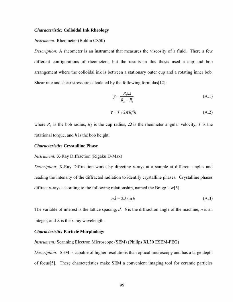
99

Characteristic: Colloidal Ink Rheology

Instrument: Rheometer (Bohlin CS50)

Description: A rheometer is an instrument that measures the viscosity of a fluid. There a few

different configurations of rheometers, but the results in this thesis used a cup and bob

arrangement where the colloidal ink is between a stationary outer cup and a rotating inner bob.

Shear rate and shear stress are calculated by the following formulas[12]:

2

2 1

RR R

γ Ω=−

(A.1)

21/ 2T R hτ π= (A.2)

where R1 is the bob radius, R2 is the cup radius, Ω is the rheometer angular velocity, T is the

rotational torque, and h is the bob height.

Characteristic: Crystalline Phase

Instrument: X-Ray Diffraction (Rigaku D-Max)

Description: X-Ray Diffraction works by directing x-rays at a sample at different angles and

reading the intensity of the diffracted radiation to identify crystalline phases. Crystalline phases

diffract x-rays according to the following relationship, named the Bragg law[5].

2 sinn dλ θ= (A.3)

The variable of interest is the lattice spacing, d. θ is the diffraction angle of the machine, n is an

integer, and λ is the x-ray wavelength.

Characteristic: Particle Morphology

Instrument: Scanning Electron Microscope (SEM) (Philips XL30 ESEM-FEG)

Description: SEM is capable of higher resolutions than optical microscopy and has a large depth

of focus[5]. These characteristics make SEM a convenient imaging tool for ceramic particles

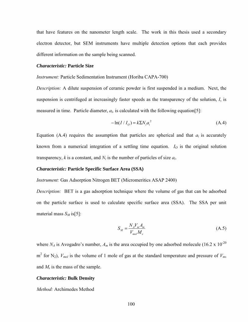
100

that have features on the nanometer length scale. The work in this thesis used a secondary

electron detector, but SEM instruments have multiple detection options that each provides

different information on the sample being scanned.

Characteristic: Particle Size

Instrument: Particle Sedimentation Instrument (Horiba CAPA-700)

Description: A dilute suspension of ceramic powder is first suspended in a medium. Next, the

suspension is centrifuged at increasingly faster speeds as the transparency of the solution, I, is

measured in time. Particle diameter, ai, is calculated with the following equation[5]:

2ln( / )O i iI I k N a− = Σ (A.4)

Equation (A.4) requires the assumption that particles are spherical and that ai is accurately

known from a numerical integration of a settling time equation. IO is the original solution

transparency, k is a constant, and Ni is the number of particles of size ai.

Characteristic: Particle Specific Surface Area (SSA)

Instrument: Gas Adsorption Nitrogen BET (Micromeritics ASAP 2400)

Description: BET is a gas adsorption technique where the volume of gas that can be adsorbed

on the particle surface is used to calculate specific surface area (SSA). The SSA per unit

material mass SM is[5]:

A m mM

mol s

N V ASV M

= (A.5)

where NA is Avogadro’s number, Am is the area occupied by one adsorbed molecule (16.2 x 10-20

m2 for N2), Vmol is the volume of 1 mole of gas at the standard temperature and pressure of Vm,

and Ms is the mass of the sample.

Characteristic: Bulk Density

Method: Archimedes Method

101

Description: Archimedes method uses the buoyancy of the sample to calculate bulk density, B,

of the structure[13]:

DBM S

=−

(A.6)

where D is the dry sample mass, M is the mass of the sample when saturated with water, and S is

the measured mass of the saturated sample when suspended is water.

Characteristic: Theoretical Density

Instrument: Helium Pycnometer (Micromeritics 1330)

Description: Helium pycnometry is used when a significant portion of the particles are smaller

than 10 μm. Gas is intruded into the sample that is sitting in a cup of a calibrated volume.

Theoretical density is determined by comparing the volume of gas intruded, cup volume, and

sample mass[5].

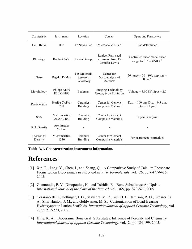
102

Chacteristic Instrument Location Contact Operating Parameters

Ca/P Ratio ICP 47 Noyes Lab Microanalysis Lab Lab determined

Rheology Bohlin CS-50 Lewis Group Ranjeet Rao, need

permission from Dr. Jennifer Lewis

Controlled shear mode, shear range 6x10-2 – 650 s-1

Phase Rigaku D-Max 148 Materials

Research Laboratory

Center for Microanalysis of

Materials

2θ range = 20 - 80°, step size = 0.048°

Morphology Philips XL30 ESEM-FEG Beckman Imaging Technology

Group, Scott Robinson Voltage = 5.00 kV, Spot = 2.0

Particle Size Horiba CAPA-700

Ceramics Building

Center for Cement Composite Materials

Dmax = 100 μm, Dmin = 0.3 μm, Div = 0.1 μm.

SSA Micromeritics ASAP 2400

Ceramics Building

Center for Cement Composite Materials 7 point analysis

Bulk Density Archimedes Method - - -

Theoretical Density

Micromeritics 1330

Ceramics Building

Center for Cement Composite Materials Per instrument instructions

Table A.1. Characterization instrument information.

References [1] Xin, R., Leng, Y., Chen, J., and Zhang, Q., A Comparitive Study of Calcium Phosphate

Formation on Bioceramics In Vitro and In Vivo Biomaterials, vol. 26, pp. 6477-6486, 2005.

[2] Giannoudis, P. V., Dinopoulos, H., and Tsiridis, E., Bone Substitutes: An Update International Journal of the Care of the Injured, vol. 36S, pp. S20-S27, 2005.

[3] Cesarano III, J., Dellinger, J. G., Saavedra, M. P., Gill, D. D., Jamison, R. D., Grosser, B. A., Sinn-Hanlon, J. M., and Goldwasser, M. S., Customization of Load-Bearing Hydroxyapatite Lattice Scaffolds Internation Journal of Applied Ceramic Technology, vol. 2, pp. 212-220, 2005.

[4] Hing, K. A., Bioceramic Bone Graft Substitutes: Influence of Porosity and Chemistry International Journal of Applied Ceramic Technology, vol. 2, pp. 184-199, 2005.

103

[5] Reed, J. S. Introduction to the Principles of Ceramic Processing, United States of America : John Wiley & Sons, Inc., 1987.

[6] Vanderbilt Technical Data RV-05-10, Darvan 821A, R.T. Vanderbilt Company, Inc.

[7] Lewis, J. A. , Colloidal Processing of Ceramics Journal of the American Ceramic Society, vol. 83, pp. 2341-2359, 2000.

[8] Dow Chemical Company, METHOCEL Cellulose Ethers Dow Chemical. USA.

[9] Smay, J. E., Cesarano III, J., and Lewis, J. A., Colloidal Inks for Directed Assembly of 3-D Periodic Structures Langmuir, vol. 18, pp. 5429-5437, 2002.

[10] Michna, S., Wu, W., and Lewis, J. A., Concentrated hydroxyapatite inks for direct-write assembly of 3-D periodic scaffolds Biomaterials, vol. 26, pp. 5632-5639, 2005.

[11] Wang, H., Lee, J.-K., Moursi, A., and Lannutti, J. J., Ca/P Ratio Effects on the Degradation of Hydroxyapatite In Vitro Journal of Biomedical Materials Research Part A, vol. 67A, pp. 599-608, 2003.

[12] Chhabra, R. and Richardson, J., Non-Newtonian Flow in the Process Industries pp. 5-161, 1999. Butterworth-Heinemann. Oxford, UK.

[13] Standard Test Method for Water Absorption, Bulk Density, Apparent Porosity, and Apparent Specific Gravity of Fired Whiteware Products ASTM International, 1999. C 373 - 88.

104

Appendix B Ink Fabrication Protocol

Last updated: 11-12-07 by David Hoelzle Written by Sheeny Lan and David Hoelzle General Notes

- Ink performance, and viscosity, is most sensitive to the solids loading. Make sure to scrape all solids from weighboats as best possible to minimize sources of error. Also, take extra care when weighing the wet and dry samples after centrifuging.

- Do not fill centrifuge tubes all the way up. The higher level causes a high level of solid separation, causing agglomerates to form. Limit centrifuge fill to 2/3rds full.

- The pH meter from the Jamison lab is much more accurate and repeatable than the Alleyne pH meter. Use the Jamison lab pH meter whenever possible.

- Send your completed spreadsheets back to Dave Hoelzle so he can keep them on record.

Day 1

1. Calcine powders for 10 hours at 1100C using the large furnace in 111 MEB. Contact Dave Hoelzle concerning use of kiln if it is your first time.

Day 2

2. AM. Ball mill for 14 hours in ethanol - Use mill in basement of ceramics building - Add 150 g HA and 300 mL of ethanol with all the grinding media into large ball

milling Nalgene jar. Ball milling Nalgene jar has been turned black from multiple ball milling operations, only use this jar.

- Place jar into can and tape opening so that jar cannot fall out of can 3. Place a sieve over a cake pan - pour HA suspension and media out of bottle onto sieve

and rinse out bottle with ethanol. 4. Rinse sieve and media well with ethanol such that most of the HA is flushed into the cake

pan 5. Put pan in drying oven (MSEB 3203) to allow powder to dry (~ 1 day at higher

temperature settings) Day 3

6. A good reference paper is Michna, S., Wu, W., Lewis, J.A., “Concentrated hydroxyapatite inks for direct-write assembly of 3-D periodic scaffolds,” Biomaterials, 26 (2005) pp. 5632-5639. Procedure follows paper except for the addition of PMMA, filtering step, and pH target value.

105

7. Based on the mass of HA powder needed, use spreadsheet to determine volume of water and Darvan 821A to add. Contact Dave Hoelzle for spreadsheet. Generic spreadsheet has been added to ABBLab gmail account.

8. Grab a clean beaker and put in water and appropriate amount of Darvan 821A with magnetic mixing bar

9. Adjust pH to 10 using 5M NH4OH. Increments depend on size of batch. Point of reference: 100g HA batch requires ~ 900 μL of base to reach pH 10.

10. Add 1/3 of HA powder. 11. Put parafilm over the beaker opening and sonicate for 3 min. 12. Add next 1/3 of HA powder and sonicate 13. Add last 1/3 of HA powder and sonicate 14. Slowly pour HA mixture from beaker into a Nalgene bottle (can add DI water to get

remaining HA out of beaker) 15. Put bottle on paint shaker for 50 minutes 16. Sonicate for 4 min. 17. Transfer slurry into centrifuge tubes such that all tubes are filled with the same volume

(can use DI water to rinse remaining HA out of bottle). Do not fill centrifuge tubes more than 2/3 full. Overly filled centrifuge tubes cause too much separation and particle consolidation occurs prematurely.

18. Centrifuge at 2000 rpm for 60 min. 19. Rinse out Nalgene bottle, put tape on bottle and label it, add media (2) – measure mass of

bottle (with lid on) – record 20. Pour excess water from centrifuge tubes and then scoop HA out into bottle 21. Put bottle on paint shaker for 60 minutes 22. Mass a small weighboat 23. Take ~ 2 gram sample and put into weighboat (record relevant masses on spreadsheet) 24. Store bottle of HA in fridge 25. Place weightboat sample into furnace at 35C for at least 12 hours

Day 4

26. Measure mass of weighboat + dry sample and calculate HA solids loading/volume percent

27. Using spreadsheet determine mass of PMMA, volume of additional water needed, Methocel, and 1-Octanol

28. Add in PMMA (mass out in weighboat and then transfer) 29. Add water (with pipette) 30. Add methocel (with bottle on balance) 31. Add 1-octanol (with pipette) 32. Place on paint shaker for 30 minutes 33. Add HNO3 to decrease pH and increase viscosity (viscosity is what is most important

here) – add HNO3 10-20 μL at a time – measure pH and shake for 10 minutes between additions. Addition increments based on ink volume.

34. When viscosity seems about right, add 50 – 100 μL of PEI and then shake for 10 minutes

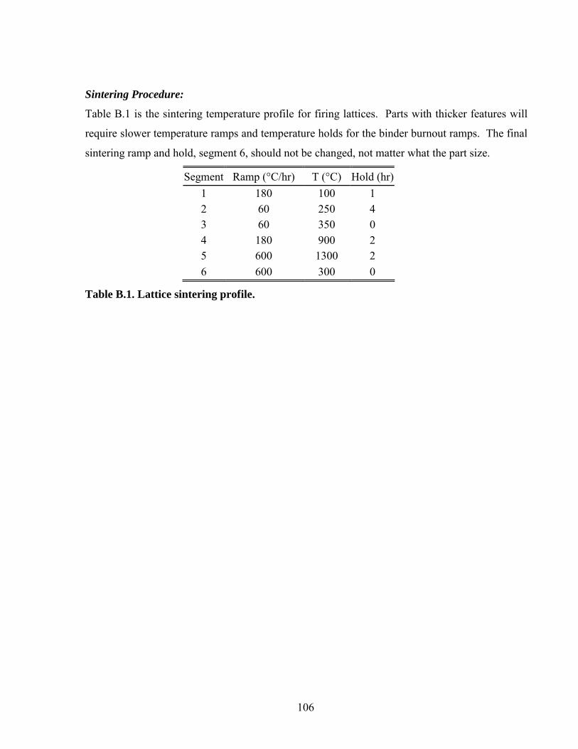
106

Sintering Procedure:

Table B.1 is the sintering temperature profile for firing lattices. Parts with thicker features will

require slower temperature ramps and temperature holds for the binder burnout ramps. The final

sintering ramp and hold, segment 6, should not be changed, not matter what the part size.

Segment Ramp (°C/hr) T (°C) Hold (hr)1 180 100 1 2 60 250 4 3 60 350 0 4 180 900 2 5 600 1300 2 6 600 300 0

Table B.1. Lattice sintering profile.

107

Appendix C Deposition Protocol

Last updated: 11-12-07 by David Hoelzle Written by Amanda Hilldore and David Hoelzle

Warnings: • Familiarize yourself with the Emergency Stops (E-Stop). These are the red buttons

located on each side of the robot. When the E-Stop is hit, all power is cut off to the micro-Robotic Deposition (mRD) machine. After an E-Stop has been hit, the buttons have to be turned to be deactivated then the machine has to be reset at the Power On location.

• The linear motors which drive the stages on the mRD machine are very powerful and can move the stages at speeds greater than 1 m/s. This is more than enough to kill you. Never stick your head in the mRD with the amplifiers activated. The amplifiers are activated when you click the Start button in the WinCon Server.

• If you have a problem that is not addressed in this protocol, you think you’ve broke something, or you are not sure what to do, do not hesitate to find or call Dave Hoelzle. No matter what time of the day. It is much better to solve your problem correctly then to put the mRD out of commission for a few weeks. Dave’s cell phone number is 614-256-7388 and his office number is 217-244-6556.

• Please do not modify the mRD or computer interface without first contacting Dave Hoelzle.

Robot Layout: The mRD and interface was designed to be a customizable controls test bed and is therefore not very user friendly. To help the user quickly understand some of the caveats of the mRD operation, this section provides a general overview. Detailed step-by-step instructions will be given in the procedure section. Below are layouts for robot space (Figure C.1), WinCon Interface (Figure C.2), Graphical User Interface (GUI) (Figure C.3), and Matlab Simulink diagram (Figure C.4). SOFTWARE OVERVIEW:

The mRD is controlled using a graphical program called Simulink, which is embedded in the program Matlab. Another program, Wincon, is used to interact between Simulink and the physical robot.

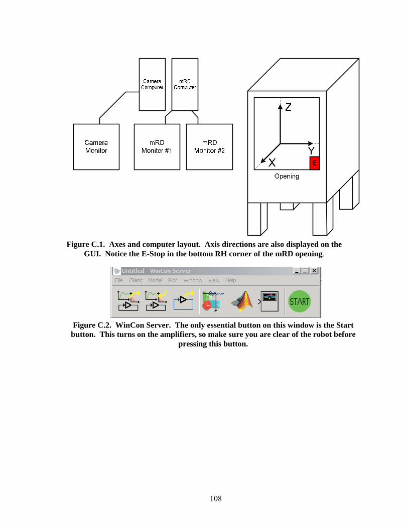
108

Figure C.1. Axes and computer layout. Axis directions are also displayed on the GUI. Notice the E-Stop in the bottom RH corner of the mRD opening.

Figure C.2. WinCon Server. The only essential button on this window is the Start button. This turns on the amplifiers, so make sure you are clear of the robot before

pressing this button.

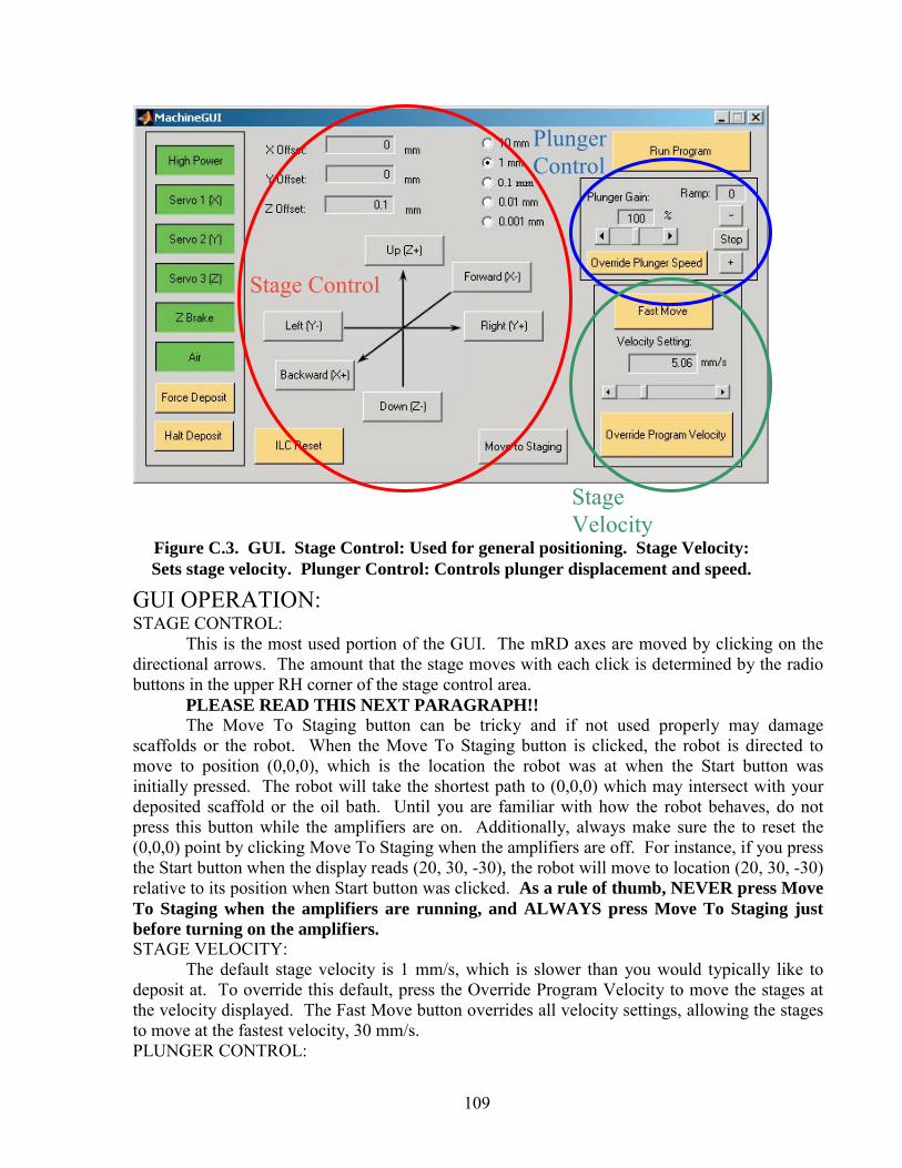
109

GUI OPERATION: STAGE CONTROL:

This is the most used portion of the GUI. The mRD axes are moved by clicking on the directional arrows. The amount that the stage moves with each click is determined by the radio buttons in the upper RH corner of the stage control area. PLEASE READ THIS NEXT PARAGRAPH!!

The Move To Staging button can be tricky and if not used properly may damage scaffolds or the robot. When the Move To Staging button is clicked, the robot is directed to move to position (0,0,0), which is the location the robot was at when the Start button was initially pressed. The robot will take the shortest path to (0,0,0) which may intersect with your deposited scaffold or the oil bath. Until you are familiar with how the robot behaves, do not press this button while the amplifiers are on. Additionally, always make sure the to reset the (0,0,0) point by clicking Move To Staging when the amplifiers are off. For instance, if you press the Start button when the display reads (20, 30, -30), the robot will move to location (20, 30, -30) relative to its position when Start button was clicked. As a rule of thumb, NEVER press Move To Staging when the amplifiers are running, and ALWAYS press Move To Staging just before turning on the amplifiers. STAGE VELOCITY: The default stage velocity is 1 mm/s, which is slower than you would typically like to deposit at. To override this default, press the Override Program Velocity to move the stages at the velocity displayed. The Fast Move button overrides all velocity settings, allowing the stages to move at the fastest velocity, 30 mm/s. PLUNGER CONTROL:

Figure C.3. GUI. Stage Control: Used for general positioning. Stage Velocity: Sets stage velocity. Plunger Control: Controls plunger displacement and speed.

Stage Control

Stage Velocity

Plunger Control

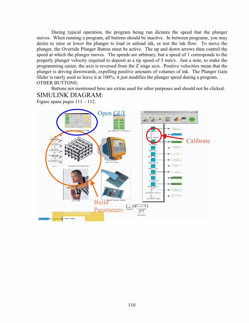
110

During typical operation, the program being run dictates the speed that the plunger moves. When running a program, all buttons should be inactive. In between programs, you may desire to raise or lower the plunger to load or unload ink, or test the ink flow. To move the plunger, the Override Plunger Button must be active. The up and down arrows then control the speed at which the plunger moves. The speeds are arbitrary, but a speed of 1 corresponds to the properly plunger velocity required to deposit at a tip speed of 5 mm/s. Just a note, to make the programming easier, the axis is reversed from the Z stage axis. Positive velocities mean that the plunger is driving downwards, expelling positive amounts of volumes of ink. The Plunger Gain Slider is rarely used so leave it at 100%; it just modifies the plunger speed during a program. OTHER BUTTONS: Buttons not mentioned here are extras used for other purposes and should not be clicked. SIMULINK DIAGRAM: Figure spans pages 111 – 112.

Calibrate

Build Parameters

Open GUI

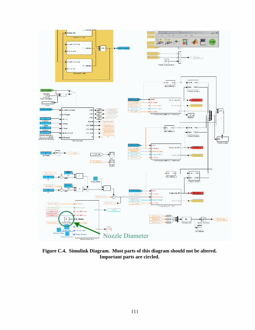
111

Figure C.4. Simulink Diagram. Most parts of this diagram should not be altered. Important parts are circled.

Nozzle Diameter

112

SIMULINK DIAGRAM OPERATION: OPEN GUI: Double clicking this box opens the GUI. If the GUI is already open and you try to open a second GUI the program will give you an error. This is mentioned again in the Troubleshooting Section. BUILD PARAMETERS: These boxes set the dimensions of the scaffold you want to build in mm units. After the appropriate units are entered, the scaffold picture must be double clicked to build the vector V. V is an ordered list of points which the robot must hit to complete the part. If V is not recalculated after the entries in the box have changed, the robot will compute the trajectory based on the previously stored V, and incorrectly build the new part. After double clicking the scaffold icon, the vector V will then be displayed in the Matlab Command window. If after depositing a scaffold of one dimension and you wish to change dimensions, you must double click the scaffold image to rebuild the vector V. Also, you will have to rebuild using WinCon; described in the procedure section. CALIBRATE: The operation of this section is described in the Trouble Shooting section. In general this box should always be set to 0. NOZZLE DIAMETER: For proper deposition, the correct nozzle diameter in mm must be entered in this box.

DEPOSITION PROCEDURE:

1. Loading ink into a syringe a. Wrap orange barrel tip cap with Teflon tape and thread onto the bottom of the

syringe. b. Put lamp oil in the syringe and coat the walls. Discard extra. c. Add ink. The amount depends on the lattice being made. d. Put the snap cap on. e. Centrifuge at 3000 rpm for 5 min

i. Make sure to counter-balance with water if necessary ii. Screw the syringe into the cap of the centrifuge tube.

2. Prep machine a. Clean stainless steel plate with ethanol b. Spray stainless steel plate with an even coat of hairspray c. Let plate dry d. Put washers over holes in oil bath (4 corners) e. Put plate on top f. Tighten with thumb screws. g. Fill bath with oil.

i. Fill all the way for tall (8mm) scaffolds. 3. Turn on machine

a. Push the power on button b. Wait a few seconds c. Push the power on button again. The green light on the top should be lit.

113

4. Prep computer a. Open Matlab 6.1

i. Make ‘D://hoelze2/DaveDeposition w/o ILC’ the current directory ii. Double click ‘Rectangular_Lattice.mdl’

iii. Things that might need to be changed 1. tip diameter: .51 2. ILC = off = 0

Goldwasser Amy Tip .51 .51 Rows 31 25 Columns 17 13 Layers 28 28 Row spacing .96 .96 Layer height .390 .390 Use ILC 0 0

iv. Double click scaffold picture 1. Make sure “V” is built 2. Wincon (at the top menu) Clean 3. Wincon Build

v. Double click GUI icon 1. Make sure X, Y, and Z offsets = 0,0,0.1!!

a. If not, click “move to staging” b. To start the camera (Left computer)

i. Start Programs ATI Multimedia TV ii. Click the setup button that looks like a checkmark

1. Stills gallery Browse My Documents\Lattices\Folder labeled as the current date

5. Get ink ready a. Add syringe to machine

i. Take snap cap off ii. Put a red plunger in

iii. Push down with allen wrench until air is gone but ink isn’t coming out. iv. Take off orange bottom with the Teflon tape v. Screw on a tip with the right diameter (0.51 = purple)

vi. Put syringe as high as possible in machine by the plunger vii. Latch in place

viii. Manually move robot head to about the correct XY location b. Recheck offsets (X,Y,Z) Offsets = (0,0,0.1) c. Click “start” d. Put tip in oil relatively quickly so ink doesn’t dry out (not too far down in the oil

bath though). e. Move tip to starting location (off plate if at the top or away from where scaffolds

will be made) f. Shine light at tip g. Move camera to tip and focus

114

i. Camera does not react well to high intensity light. If screen flickers blue, adjust the light or camera aperture to be dimmer.

h. Get air out and check ink i. Click “override plunger speed”

ii. Run at 5 until the first air bubble or ink comes out iii. Click stop iv. Run at 1 to see how ink behaves

1. Let it run for a while 2. Ideally see individual rows that form a cone

v. Then translate the tip and see 1. how much the ink stretches (more = good) 2. if the cone tips over (good)

i. Move the tip to the plate, but not the starting position j. Zero the tip

i. Move camera to tip ii. A light above the closest E-Stop indicates when the tip is contacting the

substrate. Using the system is optional, with practice the tip can be accurately zeroed by sight. If you use the light system, make sure the nozzle tip is clean because ink does not conduct electricity well.

iii. Zeroing the tip is an iterative process. First start by getting the tip close to the substrate in 1mm increments. When the tip is close switch to 0.1mm increments and move until you contact the plate. Once the tip is within 0.1mm increments, switch to 0.01mm increments until tip is once again just touching the substrate. Being within 0.01mm is good enough for this process.

iv. Once zeroed, you must move the tip up to the proper fly height. Move the Z axis up 0.77 times the nozzle diameter in mm for the 1st layer.

k. Fast lines (Optional, used for testing the ink) i. Unclick “fast move” (Velocity should be at 5 mm/s)

ii. Change to 1mm increments iii. Make sure override plunger is on iv. Change the plunger speed to 1 v. Move nozzle to make sure you have a good line.

6. Starting lattice a. Move tip to where you want the upper left corner of the scaffold to be.

i. Don’t forget about the lead in lines – don’t put the tip too close to the thumb screws or the edge of the plate.

115

Width

Hei

ght

15 m

m

Width

Nozzle PositionAt Start Program

b. Unclick override plunger speed c. Run program d. Move camera after lead-in lines and take pictures.

7. Ending lattice a. When the lattice if finished, move the tip in the +z and –x directions. This is

because when Run Program is inactivated, the tip will return to the position at which Run Program was activated at, and will drag through your part.

b. Click “run program” c. Click “override plunger speed” d. Change the plunger speed to –(75-100). e. Click stop when the plunger reaches the top starting position

i. WARNING: there are no safety stops currently installed, so make sure to not go too far.

f. Click stop g. Manually move the head close to you (and not over the oil bath) h. Remove and discard syringe.

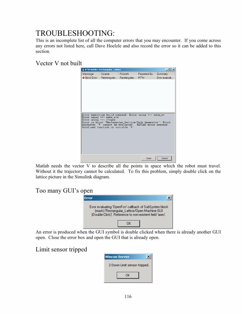
116

TROUBLESHOOTING: This is an incomplete list of all the computer errors that you may encounter. If you come across any errors not listed here, call Dave Hoelzle and also record the error so it can be added to this section. Vector V not built

Matlab needs the vector V to describe all the points in space which the robot must travel. Without it the trajectory cannot be calculated. To fix this problem, simply double click on the lattice picture in the Simulink diagram. Too many GUI’s open

An error is produced when the GUI symbol is double clicked when there is already another GUI open. Close the error box and open the GUI that is already open. Limit sensor tripped

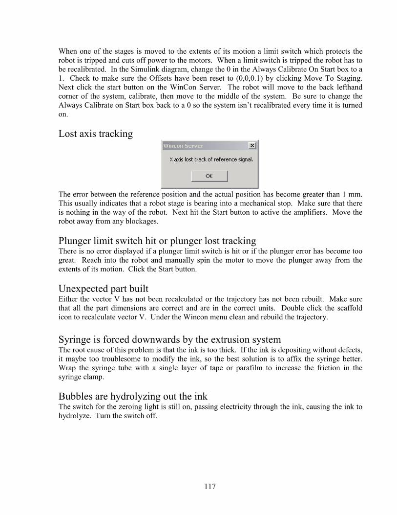
117

When one of the stages is moved to the extents of its motion a limit switch which protects the robot is tripped and cuts off power to the motors. When a limit switch is tripped the robot has to be recalibrated. In the Simulink diagram, change the 0 in the Always Calibrate On Start box to a 1. Check to make sure the Offsets have been reset to (0,0,0.1) by clicking Move To Staging. Next click the start button on the WinCon Server. The robot will move to the back lefthand corner of the system, calibrate, then move to the middle of the system. Be sure to change the Always Calibrate on Start box back to a 0 so the system isn’t recalibrated every time it is turned on. Lost axis tracking

The error between the reference position and the actual position has become greater than 1 mm. This usually indicates that a robot stage is bearing into a mechanical stop. Make sure that there is nothing in the way of the robot. Next hit the Start button to active the amplifiers. Move the robot away from any blockages. Plunger limit switch hit or plunger lost tracking There is no error displayed if a plunger limit switch is hit or if the plunger error has become too great. Reach into the robot and manually spin the motor to move the plunger away from the extents of its motion. Click the Start button. Unexpected part built Either the vector V has not been recalculated or the trajectory has not been rebuilt. Make sure that all the part dimensions are correct and are in the correct units. Double click the scaffold icon to recalculate vector V. Under the Wincon menu clean and rebuild the trajectory. Syringe is forced downwards by the extrusion system The root cause of this problem is that the ink is too thick. If the ink is depositing without defects, it maybe too troublesome to modify the ink, so the best solution is to affix the syringe better. Wrap the syringe tube with a single layer of tape or parafilm to increase the friction in the syringe clamp. Bubbles are hydrolyzing out the ink The switch for the zeroing light is still on, passing electricity through the ink, causing the ink to hydrolyze. Turn the switch off.

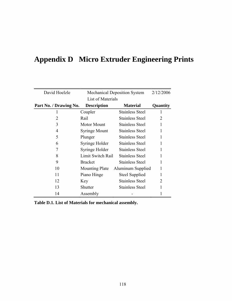
118

Appendix D Micro Extruder Engineering Prints

David Hoelzle Mechanical Deposition System 2/12/2006 List of Materials

Part No. / Drawing No. Description Material Quantity 1 Coupler Stainless Steel 1 2 Rail Stainless Steel 2 3 Motor Mount Stainless Steel 1 4 Syringe Mount Stainless Steel 1 5 Plunger Stainless Steel 1 6 Syringe Holder Stainless Steel 1 7 Syringe Holder Stainless Steel 1 8 Limit Switch Rail Stainless Steel 1 9 Bracket Stainless Steel 1 10 Mounting Plate Aluminum Supplied 1 11 Piano Hinge Steel Supplied 1 12 Key Stainless Steel 2 13 Shutter Stainless Steel 1 14 Assembly - 1

Table D.1. List of Materials for mechanical assembly.

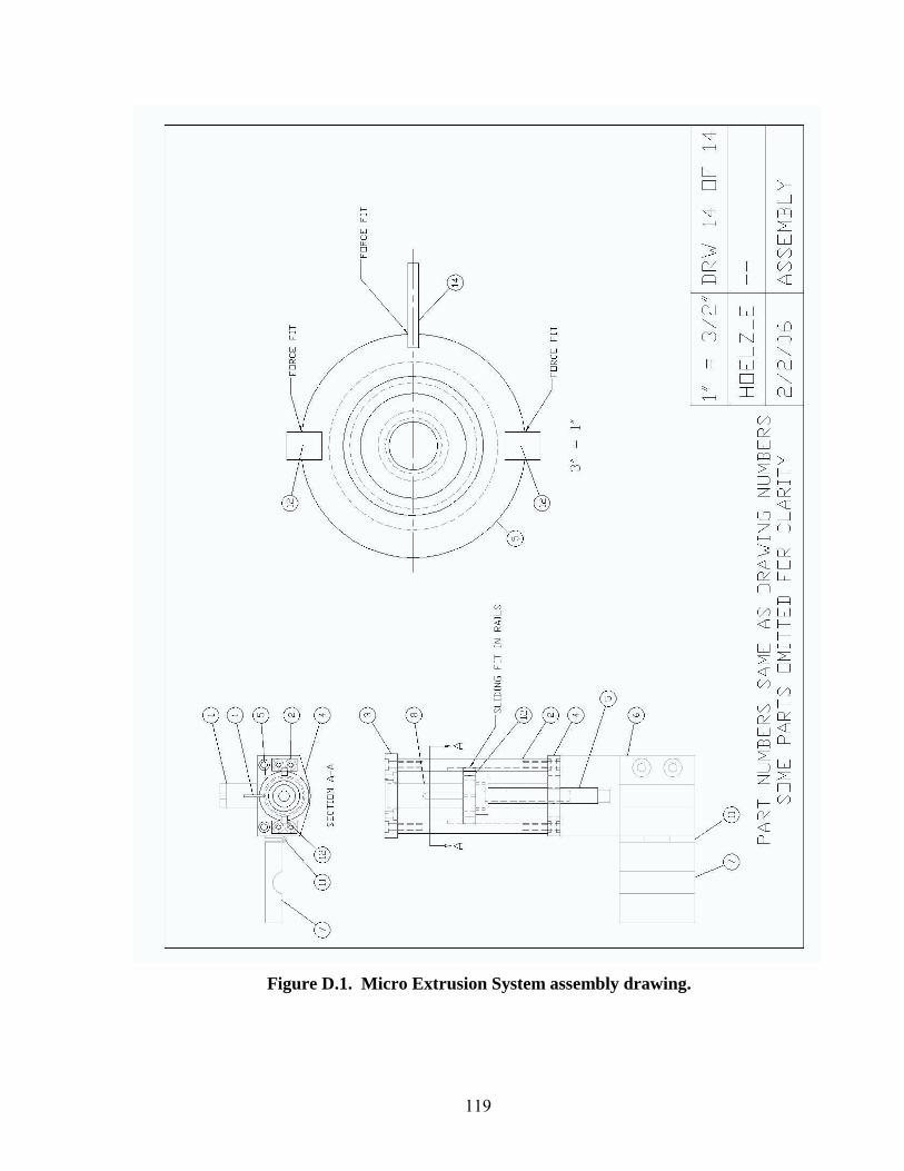
119

Figure D.1. Micro Extrusion System assembly drawing.

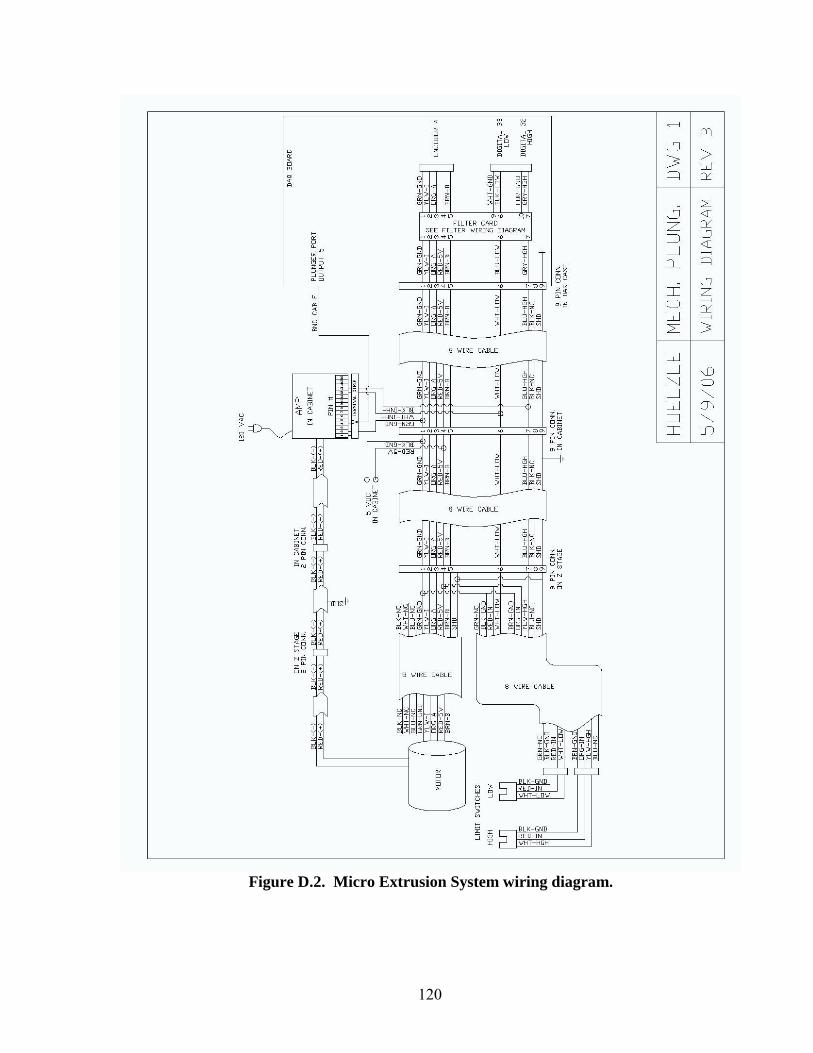
120

Figure D.2. Micro Extrusion System wiring diagram.

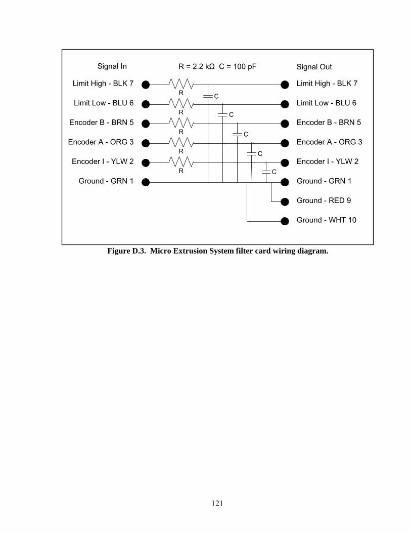
121

Limit High - BLK 7

Limit Low - BLU 6

Encoder B - BRN 5

Encoder A - ORG 3

Encoder I - YLW 2

Ground - GRN 1

RLimit High - BLK 7

Limit Low - BLU 6

Encoder B - BRN 5

Encoder A - ORG 3

Encoder I - YLW 2

Ground - GRN 1R

R

R

R

C

C

C

C

C

Signal In Signal OutR = 2.2 kΩ C = 100 pF

Ground - RED 9

Ground - WHT 10

Figure D.3. Micro Extrusion System filter card wiring diagram.

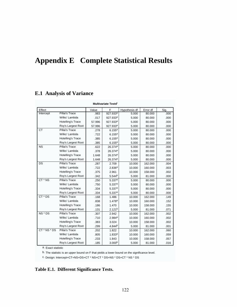
122

Appendix E Complete Statistical Results

E.1 Analysis of Variance

Multivariate Testsc

.983 927.933a 5.000 80.000 .000

.017 927.933a 5.000 80.000 .00057.996 927.933a 5.000 80.000 .00057.996 927.933a 5.000 80.000 .000

.278 6.155a 5.000 80.000 .000

.722 6.155a 5.000 80.000 .000

.385 6.155a 5.000 80.000 .000

.385 6.155a 5.000 80.000 .000

.622 26.374a 5.000 80.000 .000

.378 26.374a 5.000 80.000 .0001.648 26.374a 5.000 80.000 .0001.648 26.374a 5.000 80.000 .000.287 2.709 10.000 162.000 .004.722 2.836a 10.000 160.000 .003.375 2.961 10.000 158.000 .002.342 5.544b 5.000 81.000 .000.250 5.337a 5.000 80.000 .000.750 5.337a 5.000 80.000 .000.334 5.337a 5.000 80.000 .000.334 5.337a 5.000 80.000 .000.168 1.486 10.000 162.000 .149.838 1.478a 10.000 160.000 .152.186 1.470 10.000 158.000 .155.131 2.121b 5.000 81.000 .071.307 2.942 10.000 162.000 .002.710 2.984a 10.000 160.000 .002.383 3.024 10.000 158.000 .002.299 4.844b 5.000 81.000 .001.202 1.822 10.000 162.000 .060.805 1.833a 10.000 160.000 .059.233 1.843 10.000 158.000 .057.185 3.000b 5.000 81.000 .016

Pillai's TraceWilks' LambdaHotelling's TraceRoy's Largest RootPillai's TraceWilks' LambdaHotelling's TraceRoy's Largest RootPillai's TraceWilks' LambdaHotelling's TraceRoy's Largest RootPillai's TraceWilks' LambdaHotelling's TraceRoy's Largest RootPillai's TraceWilks' LambdaHotelling's TraceRoy's Largest RootPillai's TraceWilks' LambdaHotelling's TraceRoy's Largest RootPillai's TraceWilks' LambdaHotelling's TraceRoy's Largest RootPillai's TraceWilks' LambdaHotelling's TraceRoy's Largest Root

EffectIntercept

CT

NS

DS

CT * NS

CT * DS

NS * DS

CT * NS * DS

Value F Hypothesis df Error df Sig.

Exact statistica.

The statistic is an upper bound on F that yields a lower bound on the significance level.b.

Design: Intercept+CT+NS+DS+CT * NS+CT * DS+NS * DS+CT * NS * DSc.

Table E.1. Different Significance Tests.

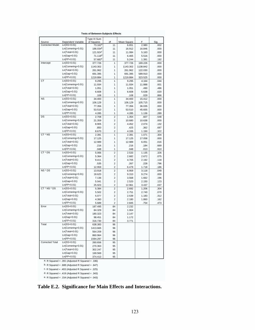
123

Tests of Between-Subjects Effects

73.162a 11 6.651 2.980 .002186.034b 11 16.912 16.846 .000121.924c 11 11.084 5.163 .00071.118d 11 6.465 5.516 .00057.682e 11 5.244 1.391 .192

377.726 1 377.726 169.226 .0001143.302 1 1143.302 1138.842 .000261.962 1 261.962 122.030 .000691.395 1 691.395 589.910 .000

1219.884 1 1219.884 323.525 .0009.295 1 9.295 4.164 .044

11.934 1 11.934 11.888 .0011.051 1 1.051 .490 .4866.608 1 6.608 5.638 .020.108 1 .108 .029 .866

34.400 1 34.400 15.412 .000106.129 1 106.129 105.715 .00077.356 1 77.356 36.035 .00053.510 1 53.510 45.655 .0004.285 1 4.285 1.136 .2892.708 2 1.354 .607 .548

21.359 2 10.680 10.638 .0008.905 2 4.452 2.074 .132.850 2 .425 .362 .697

8.670 2 4.335 1.150 .3222.391 1 2.391 1.071 .304

17.125 1 17.125 17.058 .00012.989 1 12.989 6.051 .016

.216 1 .216 .184 .669

.048 1 .048 .013 .9105.066 2 2.533 1.135 .3265.364 2 2.682 2.672 .0759.411 2 4.705 2.192 .118.535 2 .267 .228 .796

12.959 2 6.479 1.718 .18613.918 2 6.959 3.118 .04918.620 2 9.310 9.274 .0007.136 2 3.568 1.662 .1965.041 2 2.520 2.150 .123

25.923 2 12.961 3.437 .0375.384 2 2.692 1.206 .3045.502 2 2.751 2.740 .0705.077 2 2.539 1.183 .3124.360 2 2.180 1.860 .1625.689 2 2.845 .754 .473

187.495 84 2.23284.329 84 1.004

180.323 84 2.14798.451 84 1.172

316.730 84 3.771638.383 96

1413.665 96564.209 96860.964 96

1594.297 96260.656 95270.363 95302.247 95169.569 95374.413 95

Dependent VariableLn(SS+0.01)Ln(Cornering+0.01)Ln(Total+0.01)Ln(Gap+0.01)Ln(FP+0.01)Ln(SS+0.01)Ln(Cornering+0.01)Ln(Total+0.01)Ln(Gap+0.01)Ln(FP+0.01)Ln(SS+0.01)Ln(Cornering+0.01)Ln(Total+0.01)Ln(Gap+0.01)Ln(FP+0.01)Ln(SS+0.01)Ln(Cornering+0.01)Ln(Total+0.01)Ln(Gap+0.01)Ln(FP+0.01)Ln(SS+0.01)Ln(Cornering+0.01)Ln(Total+0.01)Ln(Gap+0.01)Ln(FP+0.01)Ln(SS+0.01)Ln(Cornering+0.01)Ln(Total+0.01)Ln(Gap+0.01)Ln(FP+0.01)Ln(SS+0.01)Ln(Cornering+0.01)Ln(Total+0.01)Ln(Gap+0.01)Ln(FP+0.01)Ln(SS+0.01)Ln(Cornering+0.01)Ln(Total+0.01)Ln(Gap+0.01)Ln(FP+0.01)Ln(SS+0.01)Ln(Cornering+0.01)Ln(Total+0.01)Ln(Gap+0.01)Ln(FP+0.01)Ln(SS+0.01)Ln(Cornering+0.01)Ln(Total+0.01)Ln(Gap+0.01)Ln(FP+0.01)Ln(SS+0.01)Ln(Cornering+0.01)Ln(Total+0.01)Ln(Gap+0.01)Ln(FP+0.01)Ln(SS+0.01)Ln(Cornering+0.01)Ln(Total+0.01)Ln(Gap+0.01)Ln(FP+0.01)

SourceCorrected Model

Intercept

CT

NS

DS

CT * NS

CT * DS

NS * DS

CT * NS * DS

Error

Total

Corrected Total

Type III Sumof Squares df Mean Square F Sig.

R Squared = .281 (Adjusted R Squared = .186)a.

R Squared = .688 (Adjusted R Squared = .647)b.

R Squared = .403 (Adjusted R Squared = .325)c.

R Squared = .419 (Adjusted R Squared = .343)d.

R Squared = .154 (Adjusted R Squared = .043)e.

Table E.2. Significance for Main Effects and Interactions.

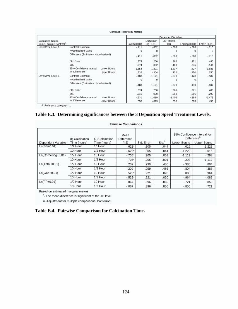
124

Contrast Results (K Matrix)

-.411 -.802 -.608 -.088 -.7160 0 0 0 0

-.411 -.802 -.608 -.088 -.716

.374 .250 .366 .271 .485

.274 .002 .100 .745 .144-1.154 -1.301 -1.337 -.627 -1.681

.332 -.304 .120 .450 .250-.188 -1.121 -.678 .140 -.507

0 0 0 0 0

-.188 -1.121 -.678 .140 -.507

.374 .250 .366 .271 .485

.616 .000 .068 .606 .299-.931 -1.619 -1.406 -.398 -1.473.555 -.623 .050 .678 .458

Contrast EstimateHypothesized ValueDifference (Estimate - Hypothesized)

Std. ErrorSig.

Lower BoundUpper Bound

95% Confidence Intervalfor Difference

Contrast EstimateHypothesized ValueDifference (Estimate - Hypothesized)

Std. ErrorSig.

Lower BoundUpper Bound

95% Confidence Intervalfor Difference

Deposition Speed(mm/s) Simple Contrasta

Level 2 vs. Level 1

Level 3 vs. Level 1

Ln(SS+0.01)Ln(Cornering+0.01)

Ln(Total+0.01) Ln(Gap+0.01) Ln(FP+0.01)

Dependent Variable

Reference category = 1a.

Table E.3. Determining significances between the 3 Deposition Speed Treatment Levels.

Pairwise Comparisons

.622* .305 .044 .016 1.229-.622* .305 .044 -1.229 -.016-.705* .205 .001 -1.112 -.298.705* .205 .001 .298 1.112.209 .299 .486 -.385 .804

-.209 .299 .486 -.804 .385.525* .221 .020 .085 .964

-.525* .221 .020 -.964 -.085.067 .396 .866 -.721 .855

-.067 .396 .866 -.855 .721

(J) CalcinationTime (hours)10 Hour1/2 Hour10 Hour1/2 Hour10 Hour1/2 Hour10 Hour1/2 Hour10 Hour1/2 Hour

(I) CalcinationTime (hours)1/2 Hour10 Hour1/2 Hour10 Hour1/2 Hour10 Hour1/2 Hour10 Hour1/2 Hour10 Hour

Dependent VariableLn(SS+0.01)

Ln(Cornering+0.01)

Ln(Total+0.01)

Ln(Gap+0.01)

Ln(FP+0.01)

MeanDifference

(I-J) Std. Error Sig.a Lower Bound Upper Bound

95% Confidence Interval forDifferencea

Based on estimated marginal meansThe mean difference is significant at the .05 level.*.

Adjustment for multiple comparisons: Bonferroni.a.

Table E.4. Pairwise Comparison for Calcination Time.

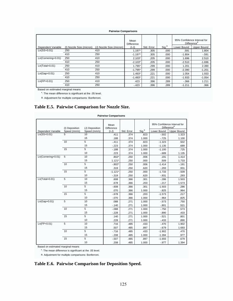
125

Pairwise Comparisons

1.197* .305 .000 .591 1.804-1.197* .305 .000 -1.804 -.5912.103* .205 .000 1.696 2.510

-2.103* .205 .000 -2.510 -1.6961.795* .299 .000 1.201 2.390

-1.795* .299 .000 -2.390 -1.2011.493* .221 .000 1.054 1.933

-1.493* .221 .000 -1.933 -1.054.423 .396 .289 -.366 1.211

-.423 .396 .289 -1.211 .366

(J) Nozzle Size (micron)410250410250410250410250410250

(I) Nozzle Size (micron)250410250410250410250410250410

Dependent VariableLn(SS+0.01)

Ln(Cornering+0.01)

Ln(Total+0.01)

Ln(Gap+0.01)

Ln(FP+0.01)

MeanDifference

(I-J) Std. Error Sig.a Lower Bound Upper Bound

95% Confidence Interval forDifferencea

Based on estimated marginal meansThe mean difference is significant at the .05 level.*.

Adjustment for multiple comparisons: Bonferroni.a.

Table E.5. Pairwise Comparison for Nozzle Size.

Pairwise Comparisons

.411 .374 .823 -.502 1.323

.188 .374 1.000 -.725 1.100-.411 .374 .823 -1.323 .502-.223 .374 1.000 -1.135 .689-.188 .374 1.000 -1.100 .725.223 .374 1.000 -.689 1.135.802* .250 .006 .191 1.414

1.121* .250 .000 .509 1.733-.802* .250 .006 -1.414 -.191.319 .250 .620 -.293 .931

-1.121* .250 .000 -1.733 -.509-.319 .250 .620 -.931 .293.608 .366 .301 -.286 1.503.678 .366 .203 -.217 1.573

-.608 .366 .301 -1.503 .286.070 .366 1.000 -.825 .964

-.678 .366 .203 -1.573 .217-.070 .366 1.000 -.964 .825.088 .271 1.000 -.573 .750

-.140 .271 1.000 -.801 .521-.088 .271 1.000 -.750 .573-.228 .271 1.000 -.890 .433.140 .271 1.000 -.521 .801.228 .271 1.000 -.433 .890.716 .485 .433 -.470 1.902.507 .485 .897 -.679 1.693

-.716 .485 .433 -1.902 .470-.208 .485 1.000 -1.394 .977-.507 .485 .897 -1.693 .679.208 .485 1.000 -.977 1.394

(J) DepositionSpeed (mm/s)10155155101015515510101551551010155155101015515510

(I) DepositionSpeed (mm/s)5

10

15

5

10

15

5

10

15

5

10

15

5

10

15

Dependent VariableLn(SS+0.01)

Ln(Cornering+0.01)

Ln(Total+0.01)

Ln(Gap+0.01)

Ln(FP+0.01)

MeanDifference

(I-J) Std. Error Sig.a Lower Bound Upper Bound

95% Confidence Interval forDifferencea

Based on estimated marginal meansThe mean difference is significant at the .05 level.*.

Adjustment for multiple comparisons: Bonferroni.a.

Table E.6. Pairwise Comparison for Deposition Speed.

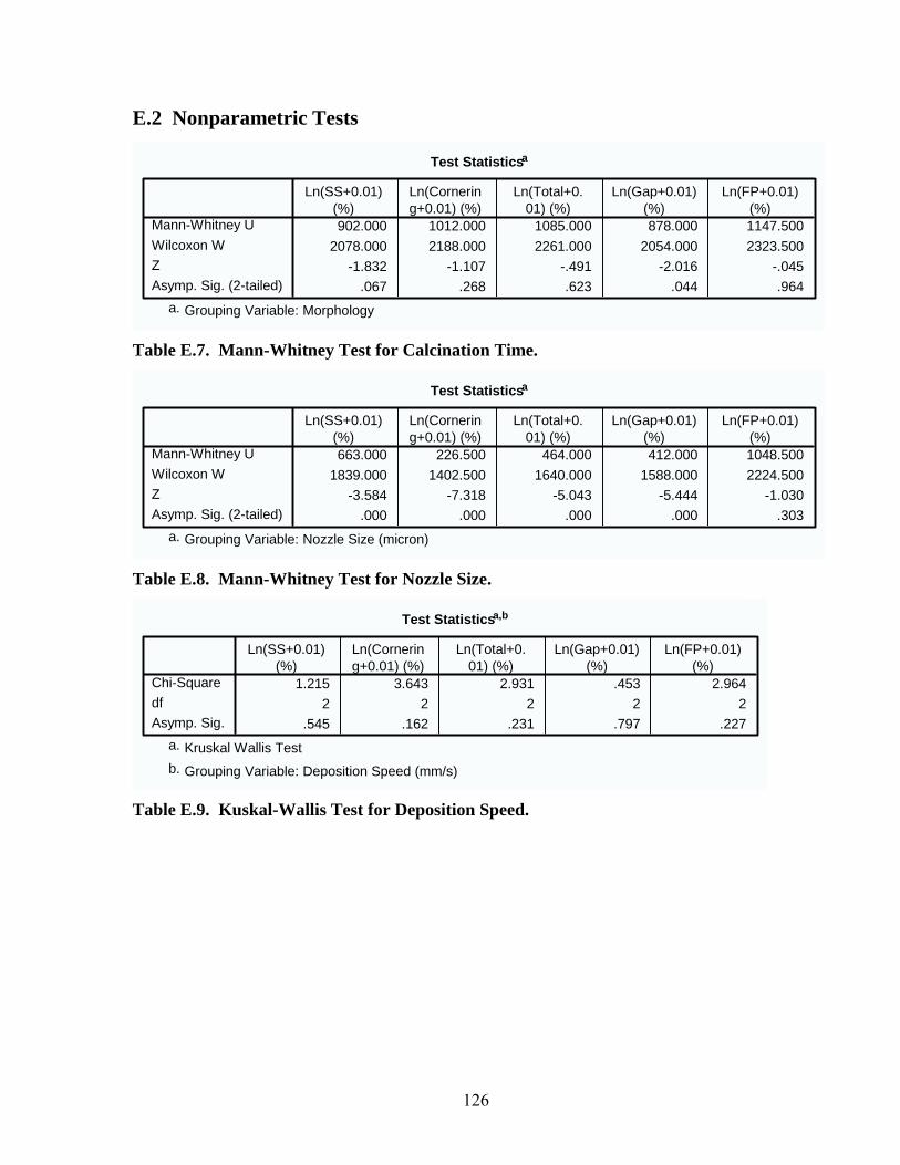
126

E.2 Nonparametric Tests

Test Statisticsa

902.000 1012.000 1085.000 878.000 1147.5002078.000 2188.000 2261.000 2054.000 2323.500

-1.832 -1.107 -.491 -2.016 -.045.067 .268 .623 .044 .964

Mann-Whitney UWilcoxon WZAsymp. Sig. (2-tailed)

Ln(SS+0.01)(%)

Ln(Cornering+0.01) (%)

Ln(Total+0.01) (%)

Ln(Gap+0.01)(%)

Ln(FP+0.01)(%)

Grouping Variable: Morphologya.

Table E.7. Mann-Whitney Test for Calcination Time.

Test Statisticsa

663.000 226.500 464.000 412.000 1048.5001839.000 1402.500 1640.000 1588.000 2224.500

-3.584 -7.318 -5.043 -5.444 -1.030.000 .000 .000 .000 .303

Mann-Whitney UWilcoxon WZAsymp. Sig. (2-tailed)

Ln(SS+0.01)(%)

Ln(Cornering+0.01) (%)

Ln(Total+0.01) (%)

Ln(Gap+0.01)(%)

Ln(FP+0.01)(%)

Grouping Variable: Nozzle Size (micron)a.

Table E.8. Mann-Whitney Test for Nozzle Size.

Test Statisticsa,b

1.215 3.643 2.931 .453 2.9642 2 2 2 2

.545 .162 .231 .797 .227

Chi-SquaredfAsymp. Sig.

Ln(SS+0.01)(%)

Ln(Cornering+0.01) (%)

Ln(Total+0.01) (%)

Ln(Gap+0.01)(%)

Ln(FP+0.01)(%)

Kruskal Wallis Testa.

Grouping Variable: Deposition Speed (mm/s)b.

Table E.9. Kuskal-Wallis Test for Deposition Speed.

127

E.3 General Loglinear Analysis Parameter Estimatesb,c

-.693 1.414 -.490 .624 -3.465 2.079-1.5E-016 2.000 .000 1.000 -3.920 3.920

0a . . . . .1.946 1.512 1.287 .198 -1.017 4.909

0a . . . . .2.565 1.468 1.748 .081 -.311 5.4411.099 1.633 .673 .501 -2.102 4.299

0a . . . . .

.762 2.102 .363 .717 -3.358 4.882

0a

. . . . .

0a

. . . . .

0a

. . . . .

-.368 2.092 -.176 .860 -4.468 3.732

2.037 2.180 .934 .350 -2.236 6.310

0a

. . . . .

0a

. . . . .

0a

. . . . .

0a

. . . . .

-2.314 1.631 -1.418 .156 -5.511 .884

-1.946 1.902 -1.023 .306 -5.674 1.783

0a

. . . . .

0a

. . . . .

0a

. . . . .

0a

. . . . .

-.982 2.328 -.422 .673 -5.544 3.580

-2.799 2.551 -1.097 .272 -7.798 2.200

0a

. . . . .

0a

. . . . .

0a

. . . . .

0a

. . . . .

0a

. . . . .

0a

. . . . .

0a

. . . . .

0a

. . . . .

0a

. . . . .

0a

. . . . .

ParameterConstant[Morphology_Hours = 0][Morphology_Hours = 1][Nozzle_Size = 250.00][Nozzle_Size = 410.00][Tip_Speed = 5.00][Tip_Speed = 10.00][Tip_Speed = 15.00][Morphology_Hours = 0]* [Nozzle_Size = 250.00][Morphology_Hours = 0]* [Nozzle_Size = 410.00][Morphology_Hours = 1]* [Nozzle_Size = 250.00][Morphology_Hours = 1]* [Nozzle_Size = 410.00][Morphology_Hours = 0]* [Tip_Speed = 5.00][Morphology_Hours = 0]* [Tip_Speed = 10.00][Morphology_Hours = 0]* [Tip_Speed = 15.00][Morphology_Hours = 1]* [Tip_Speed = 5.00][Morphology_Hours = 1]* [Tip_Speed = 10.00][Morphology_Hours = 1]* [Tip_Speed = 15.00][Nozzle_Size = 250.00] *[Tip_Speed = 5.00][Nozzle_Size = 250.00] *[Tip_Speed = 10.00][Nozzle_Size = 250.00] *[Tip_Speed = 15.00][Nozzle_Size = 410.00] *[Tip_Speed = 5.00][Nozzle_Size = 410.00] *[Tip_Speed = 10.00][Nozzle_Size = 410.00] *[Tip_Speed = 15.00][Morphology_Hours = 0]* [Nozzle_Size = 250.00]* [Tip_Speed = 5.00][Morphology_Hours = 0]* [Nozzle_Size = 250.00]* [Tip_Speed = 10.00][Morphology_Hours = 0]* [Nozzle_Size = 250.00]* [Tip_Speed = 15.00][Morphology_Hours = 0]* [Nozzle_Size = 410.00]* [Tip_Speed = 5.00][Morphology_Hours = 0]* [Nozzle_Size = 410.00]* [Tip_Speed = 10.00][Morphology_Hours = 0]* [Nozzle_Size = 410.00]* [Tip_Speed = 15.00][Morphology_Hours = 1]* [Nozzle_Size = 250.00]* [Tip_Speed = 5.00][Morphology_Hours = 1]* [Nozzle_Size = 250.00]* [Tip_Speed = 10.00][Morphology_Hours = 1]* [Nozzle_Size = 250.00]* [Tip_Speed = 15.00][Morphology_Hours = 1]* [Nozzle_Size = 410.00]* [Tip_Speed = 5.00][Morphology_Hours = 1]* [Nozzle_Size = 410.00]* [Tip_Speed = 10.00][Morphology_Hours = 1]* [Nozzle_Size = 410.00]* [Tip_Speed = 15.00]

Estimate Std. Error Z Sig. Lower Bound Upper Bound95% Confidence Interval

This parameter is set to zero because it is redundant.a.

Model: Poissonb.

Design: Constant + Morphology_Hours + Nozzle_Size + Tip_Speed + Morphology_Hours * Nozzle_Size+ Morphology_Hours * Tip_Speed + Nozzle_Size * Tip_Speed + Morphology_Hours * Nozzle_Size *Tip_Speed

c.

Table E.10. General Loglinear Analysis for Globular Defects.

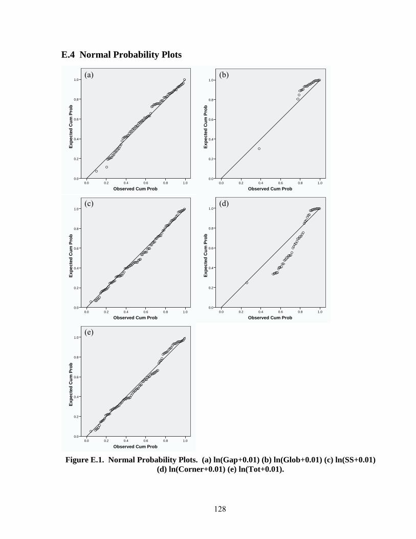
128

E.4 Normal Probability Plots

Observed Cum Prob1.00.80.60.40.20.0

Expe

cted

Cum

Pro

b

1.0

0.8

0.6

0.4

0.2

0.0

Observed Cum Prob1.00.80.60.40.20.0

Expe

cted

Cum

Pro

b

1.0

0.8

0.6

0.4

0.2

0.0

Observed Cum Prob1.00.80.60.40.20.0

Expe

cted

Cum

Pro

b

1.0

0.8

0.6

0.4

0.2

0.0

Observed Cum Prob1.00.80.60.40.20.0

Expe

cted

Cum

Pro

b1.0

0.8

0.6

0.4

0.2

0.0

Observed Cum Prob1.00.80.60.40.20.0

Expe

cted

Cum

Pro

b

1.0

0.8

0.6

0.4

0.2

0.0

Figure E.1. Normal Probability Plots. (a) ln(Gap+0.01) (b) ln(Glob+0.01) (c) ln(SS+0.01) (d) ln(Corner+0.01) (e) ln(Tot+0.01).

(a) (b)

(d) (c)

(e)

129

Appendix F Video Processing Code

Matlab m-file Video_Processing_CF (Video Processing with Correction Factor) % Syntax [TimeRef,Vdot, Error,% rod_width]=Video_Processing_CF(filename,Check_Point) function [TimeRef, Vdot1kHz, Error, rod_width] = Video_Processing_CF(filename, Check_Point); %%%%%%%%%%%%%%%%%%%%%%%%%%%%%%%%%%%%%%%%%%%%%%%%%%%%%%%%%%%%%%%%%%%%%%%%%%%%%% % This code takes the arguments of a video filename and the frame at which % to check the video to specify a region of interest and returns vectors % for time, a 1 kHz Vdot signal, a 1 kHz Error signal, and video dependent % frequency signal for rod width %%%%%%%%%%%%%%%%%%%%%%%%%%%%%%%%%%%%%%%%%%%%%%%%%%%%%%%%%%%%%%%%%%%%%%%%%%%%%% % Defined Variables used as test variables in testing % filename = 'Iteration 10.avi'; % Start_Max = 1; % Frames % Check_Point = 25; % Frames % Defined constants HorCalibrate = 83.29; %Horpixel/mm VertCalibrate = 66.20; %Vertpixel/mm PI = 3.14159; % Pi vel = 5; % mm/s h = 0.32; % mm load ReferenceSignal.mat % Pulse type input clear avi_info; clear Frame; clear mov; clear Ibw; clear Image_Gray; clear Seg_Image; clear rod_width; clear TimeTemp; clear Vdot; clear Time; % Image information avi_info = aviinfo(filename); avi_info.Filename; avi_info.FileSize; avi_info.FileModDate;

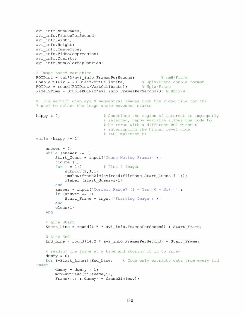
130

avi_info.NumFrames; avi_info.FramesPerSecond; avi_info.Width; avi_info.Height; avi_info.ImageType; avi_info.VideoCompression; avi_info.Quality; avi_info.NumColormapEntries; % Image based variables ROIDist = vel*3/avi_info.FramesPerSecond; % mmH/Frame DoubleROIPix = ROIDist*VertCalibrate; % Hpix/Frame double format ROIPix = round(ROIDist*VertCalibrate); % Hpix/Frame Pixel2Time = DoubleROIPix*avi_info.FramesPerSecond/3; % Hpix/s % This section displays 9 sequential images from the video file for the % user to select the image where movement starts happy = 0; % Sometimes the region of interest is improperly % selected, happy variable allows the code to % be rerun with a different ROI without % interrupting the higher level code % ILC_Implement_MI. while (happy ~= 1) answer = 0; while (answer ~= 1) Start_Guess = input('Guess Moving Frame: '); figure (1) for i = 1:9 % Plot 9 images subplot(3,3,i) imshow(frame2im(aviread(filename,Start_Guess+i-1))) xlabel (Start_Guess+i-1) end answer = input('Correct Range? (1 = Yes, 0 = No): '); if (answer == 1) Start_Frame = input('Starting Image :'); end close(1) end % Line Start Start_Line = round(1.6 * avi_info.FramesPerSecond) + Start_Frame; % Line End End_Line = round(14.2 * avi_info.FramesPerSecond) + Start_Frame; % reading one frame at a time and storing it in to array dummy = 0; for i=Start_Line:3:End_Line; % Code only extracts data from every 3rd image dummy = dummy + 1; mov=aviread(filename,i); Frame(:,:,:,dummy) = frame2im(mov);

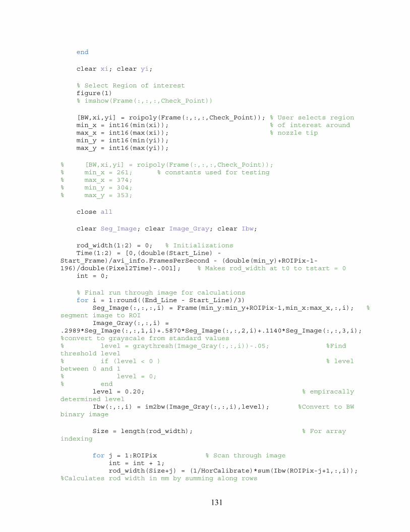
131

end clear xi; clear yi; % Select Region of interest figure(1) % imshow(Frame(:,:,:,Check_Point)) [BW,xi,yi] = roipoly(Frame(:,:,:,Check_Point)); % User selects region min_x = int16(min(xi)); % of interest around max_x = int16(max(xi)); % nozzle tip min_y = int16(min(yi)); max_y = int16(max(yi)); % [BW,xi,yi] = roipoly(Frame(:,:,:,Check_Point)); % min_x = 261; % constants used for testing % max_x = 374; % min_y = 304; % max_y = 353; close all clear Seg_Image; clear Image_Gray; clear Ibw; rod_width(1:2) = 0; % Initializations Time(1:2) = [0,(double(Start_Line) - Start_Frame)/avi_info.FramesPerSecond - (double(min_y)+ROIPix-1-196)/double(Pixel2Time)-.001]; % Makes rod_width at t0 to tstart = 0 int = 0; % Final run through image for calculations for i = 1:round((End_Line - Start_Line)/3) Seg_Image(:,:,:,i) = Frame(min_y:min_y+ROIPix-1,min_x:max_x,:,i); % segment image to ROI Image_Gray(:,:,i) = .2989*Seg_Image(:,:,1,i)+.5870*Seg_Image(:,:,2,i)+.1140*Seg_Image(:,:,3,i); %convert to grayscale from standard values % level = graythresh(Image_Gray(:,:,i))-.05; %Find threshold level % if (level < 0 ) % level between 0 and 1 % level = 0; % end level = 0.20; % empiracally determined level Ibw(:,:,i) = im2bw(Image_Gray(:,:,i),level); %Convert to BW binary image Size = length(rod_width); % For array indexing for j = 1:ROIPix % Scan through image int = int + 1; rod_width(Size+j) = (1/HorCalibrate)*sum(Ibw(ROIPix-j+1,:,i)); %Calculates rod width in mm by summing along rows

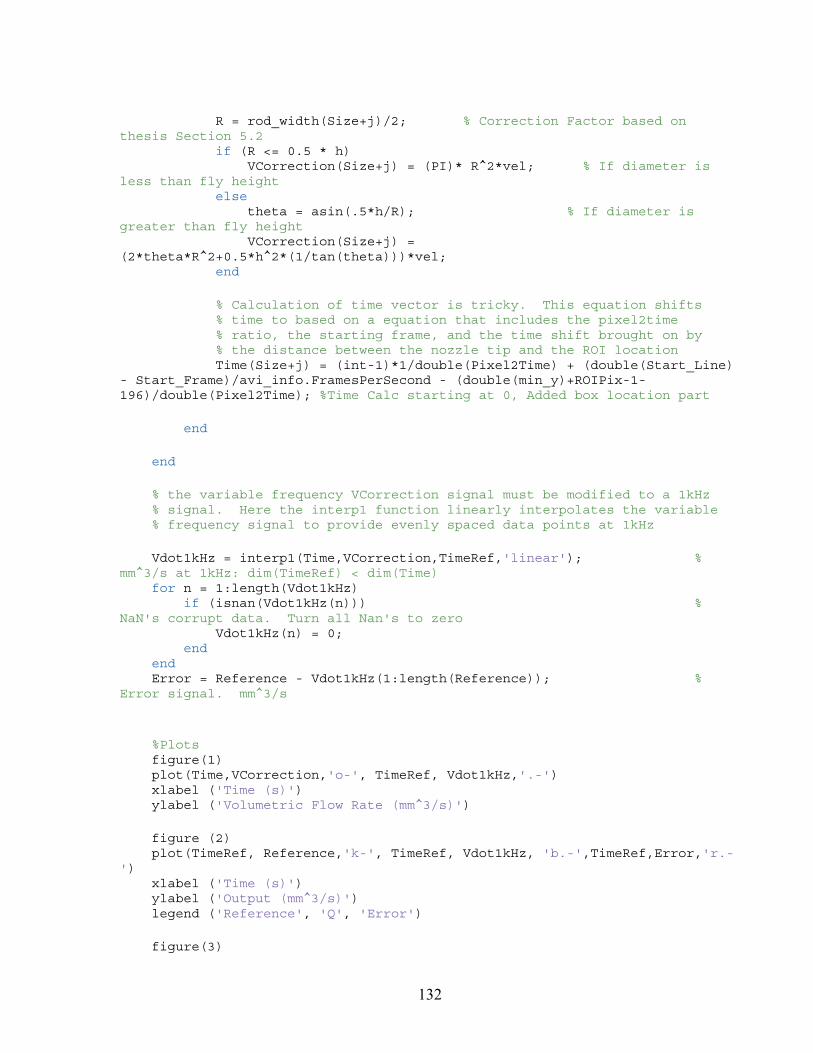
132

R = rod_width(Size+j)/2; % Correction Factor based on thesis Section 5.2 if (R <= 0.5 * h) VCorrection(Size+j) = (PI)* R^2*vel; % If diameter is less than fly height else theta = asin(.5*h/R); % If diameter is greater than fly height VCorrection(Size+j) = (2*theta*R^2+0.5*h^2*(1/tan(theta)))*vel; end % Calculation of time vector is tricky. This equation shifts % time to based on a equation that includes the pixel2time % ratio, the starting frame, and the time shift brought on by % the distance between the nozzle tip and the ROI location Time(Size+j) = (int-1)*1/double(Pixel2Time) + (double(Start_Line) - Start_Frame)/avi_info.FramesPerSecond - (double(min_y)+ROIPix-1-196)/double(Pixel2Time); %Time Calc starting at 0, Added box location part end end % the variable frequency VCorrection signal must be modified to a 1kHz % signal. Here the interp1 function linearly interpolates the variable % frequency signal to provide evenly spaced data points at 1kHz Vdot1kHz = interp1(Time,VCorrection,TimeRef,'linear'); % mm^3/s at 1kHz: dim(TimeRef) < dim(Time) for n = 1:length(Vdot1kHz) if (isnan(Vdot1kHz(n))) % NaN's corrupt data. Turn all Nan's to zero Vdot1kHz(n) = 0; end end Error = Reference - Vdot1kHz(1:length(Reference)); % Error signal. mm^3/s %Plots figure(1) plot(Time,VCorrection,'o-', TimeRef, Vdot1kHz,'.-') xlabel ('Time (s)') ylabel ('Volumetric Flow Rate (mm^3/s)') figure (2) plot(TimeRef, Reference,'k-', TimeRef, Vdot1kHz, 'b.-',TimeRef,Error,'r.-') xlabel ('Time (s)') ylabel ('Output (mm^3/s)') legend ('Reference', 'Q', 'Error') figure(3)

133

plot(Time, rod_width,'.-') xlabel ('Time (s)') ylabel ('Rod Width (mm)') happy = input('Happy with results? (0 = No, 1 = Yes): '); % Assures ROI and other things were properly chosen end Matlab m-file ILC_Implement_MI (ILC Implementation with middle iterations) % Syntax: [TimeRef, u, Error, Vdot1kHz, RMS, Max_Error] = ILC_Implement_MI(P, Bandwidth(Hz), % Order, Start Iteration, Iterations); function [TimeRefComp, u, ErrorComp, Vdot1kHzComp, rod_widthComp, RMS, Max_Error] = ILC_Implement_MI(P, Bandwidth, Order, Start_It, Iterate); %%%%%%%%%%%%%%%%%%%%%%%%%%%%%%%%%%%%%%%%%%%%%%%%%%%%%%%%%%%%%%%%%%%%%%%%%%%%%%%%%%%%%%%%% % This function uses error signals from deposition trials to calculate a % new u signal at every interation to interatively improve deposition % performance. The error signal is calculated by calling function % Video_Processing_CF.m % Input arguments are P gain, Q-filter bandwidth, Q-filter order, Starting % Iteration, and number of iterations %%%%%%%%%%%%%%%%%%%%%%%%%%%%%%%%%%%%%%%%%%%%%%%%%%%%%%%%%%%%%%%%%%%%%%%%%%%%%%%%%%%%%%%%% % Initial Parameters, variables used in testing % Start_It = 12; % Starting Iteration in event of crash % P = .5; % Proportional Gain of Learning Filter % Bandwidth = 5; % Hz, Bandwidth of Q-Filter % Order = 2; % Filter Order % Iterate = 12; % Number of Iterations % Nominal Plant Dynamics K = 0.70; % from No Control attempt 6 (Section 5.3 of thesis), Domain C tau = 1.4; % Not used, just for show num = K*[1/100 1]; % Not used, just for show den = [tau 1]; invdnum = [164.7 -164.6]; % inverse discrete plant numerator, constants calculated offline invdden = [1 -0.9048]; % inverse discrete plant denominator % Q-Filter coefficients [b,a] = butter(Order,Bandwidth/1000);

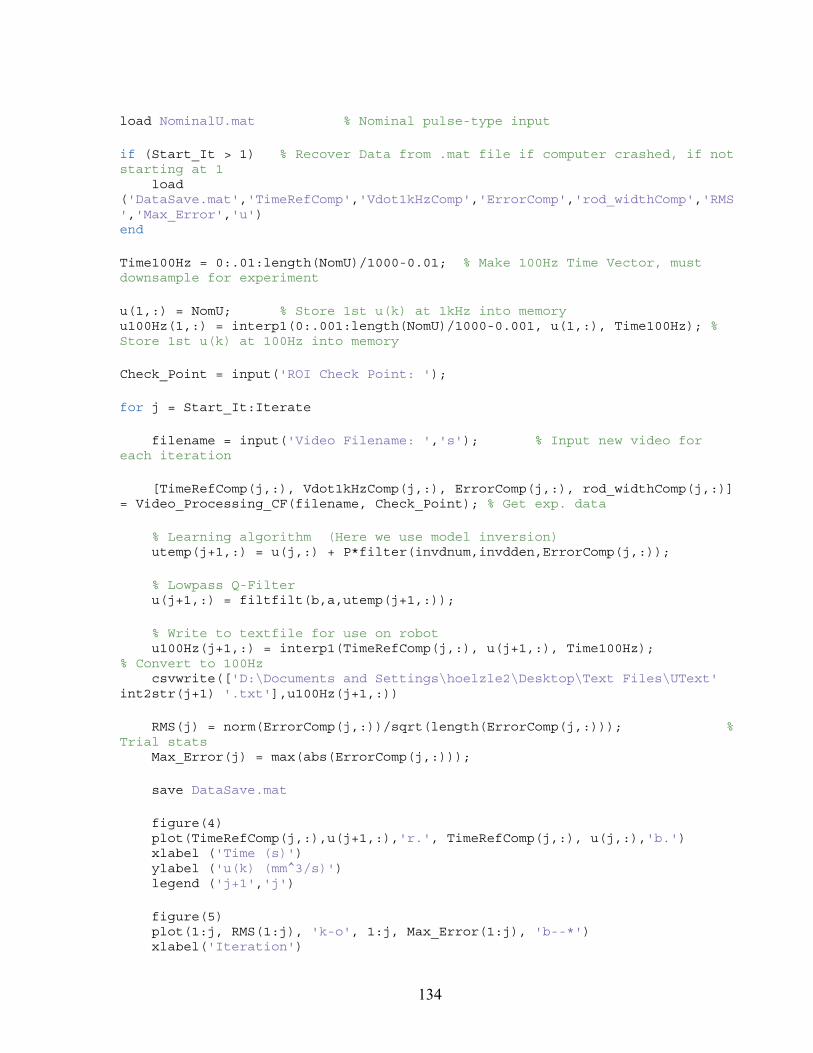
134

load NominalU.mat % Nominal pulse-type input if (Start_It > 1) % Recover Data from .mat file if computer crashed, if not starting at 1 load ('DataSave.mat','TimeRefComp','Vdot1kHzComp','ErrorComp','rod_widthComp','RMS','Max_Error','u') end Time100Hz = 0:.01:length(NomU)/1000-0.01; % Make 100Hz Time Vector, must downsample for experiment u(1,:) = NomU; % Store 1st u(k) at 1kHz into memory u100Hz(1,:) = interp1(0:.001:length(NomU)/1000-0.001, u(1,:), Time100Hz); % Store 1st u(k) at 100Hz into memory Check_Point = input('ROI Check Point: '); for j = Start_It:Iterate filename = input('Video Filename: ','s'); % Input new video for each iteration [TimeRefComp(j,:), Vdot1kHzComp(j,:), ErrorComp(j,:), rod_widthComp(j,:)] = Video_Processing_CF(filename, Check_Point); % Get exp. data % Learning algorithm (Here we use model inversion) utemp(j+1,:) = u(j,:) + P*filter(invdnum,invdden,ErrorComp(j,:)); % Lowpass Q-Filter u(j+1,:) = filtfilt(b,a,utemp(j+1,:)); % Write to textfile for use on robot u100Hz(j+1,:) = interp1(TimeRefComp(j,:), u(j+1,:), Time100Hz); % Convert to 100Hz csvwrite(['D:\Documents and Settings\hoelzle2\Desktop\Text Files\UText' int2str(j+1) '.txt'],u100Hz(j+1,:)) RMS(j) = norm(ErrorComp(j,:))/sqrt(length(ErrorComp(j,:))); % Trial stats Max_Error(j) = max(abs(ErrorComp(j,:))); save DataSave.mat figure(4) plot(TimeRefComp(j,:),u(j+1,:),'r.', TimeRefComp(j,:), u(j,:),'b.') xlabel ('Time (s)') ylabel ('u(k) (mm^3/s)') legend ('j+1','j') figure(5) plot(1:j, RMS(1:j), 'k-o', 1:j, Max_Error(1:j), 'b--*') xlabel('Iteration')

135

ylabel ('Error (mm^3/s)') legend ('RMS', 'Max Error') end