2013 Neera Jain - Ideals - University of Illinois at Urbana-Champaign

© 2013 Neera Jain

THERMODYNAMICS-BASED OPTIMIZATION AND CONTROL OF

INTEGRATED ENERGY SYSTEMS

BY

NEERA JAIN

DISSERTATION

Submitted in partial fulfillment of the requirements

for the degree of Doctor of Philosophy in Mechanical Engineering

in the Graduate College of the

University of Illinois at Urbana-Champaign, 2013

Urbana, Illinois

Doctoral Committee:

Professor Andrew Alleyne, Chair

Assistant Professor Alejandro Domínguez-García

Associate Professor Dimitrios Kyritsis

Associate Professor Srinivasa Salapaka

Professor Jakob Stoustrup, Aalborg University

ii

Abstract

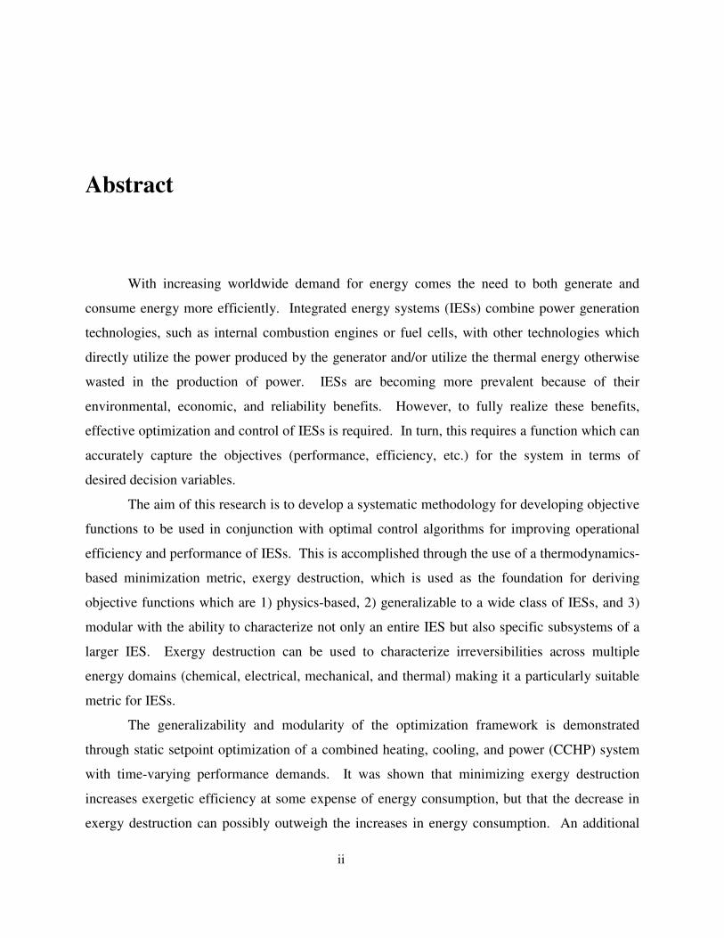
With increasing worldwide demand for energy comes the need to both generate and

consume energy more efficiently. Integrated energy systems (IESs) combine power generation

technologies, such as internal combustion engines or fuel cells, with other technologies which

directly utilize the power produced by the generator and/or utilize the thermal energy otherwise

wasted in the production of power. IESs are becoming more prevalent because of their

environmental, economic, and reliability benefits. However, to fully realize these benefits,

effective optimization and control of IESs is required. In turn, this requires a function which can

accurately capture the objectives (performance, efficiency, etc.) for the system in terms of

desired decision variables.

The aim of this research is to develop a systematic methodology for developing objective

functions to be used in conjunction with optimal control algorithms for improving operational

efficiency and performance of IESs. This is accomplished through the use of a thermodynamics-

based minimization metric, exergy destruction, which is used as the foundation for deriving

objective functions which are 1) physics-based, 2) generalizable to a wide class of IESs, and 3)

modular with the ability to characterize not only an entire IES but also specific subsystems of a

larger IES. Exergy destruction can be used to characterize irreversibilities across multiple

energy domains (chemical, electrical, mechanical, and thermal) making it a particularly suitable

metric for IESs.

The generalizability and modularity of the optimization framework is demonstrated

through static setpoint optimization of a combined heating, cooling, and power (CCHP) system

with time-varying performance demands. It was shown that minimizing exergy destruction

increases exergetic efficiency at some expense of energy consumption, but that the decrease in

exergy destruction can possibly outweigh the increases in energy consumption. An additional

iii

layer of flexibility was introduced as the “interchangeability” between power minimization and

exergy destruction rate minimization for those subsystems in which the reversible power is

constant with respect to the decision variables. Interchangeability allows the user to only derive

the exergy destruction rate for those systems in which the equivalence does not hold and

construct an objective function which would result in the same solution as minimizing the rate of

exergy destruction in every subsystem.

Exergy analyses have long been used to better understand the behavior of a variety of

thermodynamic systems, primarily from a static design and operation point of view. However,

as the complexity of integrated energy systems grows, for example as a result of intermittent grid

power from renewable energy technologies such as wind and solar, an understanding of transient

behavior is needed. As a case study, the dynamic exergy destruction rate was derived for the

refrigerant-side dynamics of a vapor-compression cycle system and then used in formulating an

exergy destruction minimization (EDM) optimal control problem for the system with full

actuation capabilities. The results highlighted how time-varying control decisions can affect the

distribution of irreversibilities throughout the overall system. Moreover, it was shown that EDM

has the potential to uncover a different set of solutions than those produced by an energy or

power minimization and is therefore a valuable tool for operational optimization of IESs.

iv

To all of my teachers.

v

Acknowledgements

First and foremost, I would like to thank my advisor, Prof. Andrew Alleyne, for his

mentorship and advice throughout the duration of my graduate career. I owe much of my

success in graduate school to him. For 7 years he has provided me with guidance and support as

I navigated through research, and life, and I have learned so much in what feels like a very short

time. I look forward to continuing to learn from him in the years ahead as I progress through my

career. I would also like to acknowledge the members of my doctoral examination committee –

Alejandro Domínguez-García, Dimitrios Kyritsis, Srinivasa Salapaka, and Jakob Stoustrup –

who have helped guide and strengthen my research with their own expertise. In particular, I

would like to thank Prof. Salapaka and Prof. Carolyn Beck who wrote letters of recommendation

on numerous occasions for me, and I thank them for their part in my success in securing valuable

fellowships throughout my graduate career.

I have been extremely fortunate to work in the Alleyne Research Group (ARG). My

peers in the ARG are among the most intelligent and kind people I have ever known. I want to

thank present and past members of the ARG who conduct research in the thermal systems area –

Vikas, Tim, Joey, Megan, Justin, Rich, and Matt – for many valuable discussions which

contributed to the work contained in this thesis. I would like to especially thank Vikas for his

help with the modeling of the CCHP system which was critical to the results presented in

Chapter 3. With respect to the results presented in Chapter 5, I want to extend a special thanks to

Bin and Joey for their expertise in the dynamic modeling of VCC systems as well as to Justin for

his help in formulating the MPC-based optimal control problem.

To the aforementioned members of the ARG as well as Kira, Dave, Nanjun, Sarah,

Sandipan, Erick, and Yangmin – thank you all for your friendship and countless hours of fun and

laughter both inside and outside of the lab. You have all been an important part of my

vi

experience at Illinois, and I hope we remain friends for many years to come. I would like to

particularly acknowledge Kira, Dave, Tim, and Vikas, with whom I have grown very close and

whose advice, both personal and professional, I have sought on many occasions. I am looking

forward to many years of friendship ahead with each of them.

Beyond research, my passion for promoting women in engineering is something that has

defined me in graduate school. I want to thank Jennifer, Helen, and Serena, who joined me in

2007 to form the first executive board of MechSE Graduate Women. I want to thank Jessie and

Sam who have each led the group as president since then, and for strengthening an organization

which continues to play an important role in the MechSE Department.

There are also many others (too many to mention) outside of the ARG who have made

my experience in graduate school more rewarding and enjoyable. Here I acknowledge three in

particular. To my friend Gayathri – thank you for your friendship and support; it has been

invaluable to share such similar experiences with one another throughout our graduate careers.

To my roommate Cathy, thank you for being the best roommate anyone could ask for, and for

being a very constant and present friend. To my husband Shreyas, thank you for your endless

encouragement, particularly through the most difficult moments in my research.

Last but not least, I want to thank my parents who have exemplified the value of hard

work and discipline throughout my life. To my siblings Bhavana and Ankush – thank you for

reminding me how to enjoy life and for your continued love and support through all of my

endeavors.

vii

Table of Contents

CHAPTER Page

List of Tables ................................................................................................................................. xi

List of Figures ............................................................................................................................... xii

List of Symbols ............................................................................................................................. xv

List of Subscripts ........................................................................................................................ xvii

List of Abbreviations ................................................................................................................... xix

1 Introduction .............................................................................................................................. 1

1.1 Integrated Energy Systems ............................................................................................. 1

1.2 Optimization and Control of IESs .................................................................................. 3

1.3 Organization of Thesis ................................................................................................... 5

2 Exergy-Based Optimization Framework ................................................................................. 7

2.1 Thermodynamic Fundamentals ...................................................................................... 7

2.2 Exergy-Based Analysis and Optimization ..................................................................... 9

2.2.1 Exergy Analysis ................................................................................................................. 9

2.2.2 Exergy Destruction Minimization ................................................................................... 10

2.2.3 Relationship Between EDM and Power Minimization .................................................... 10

2.3 EDM Framework for Integrated Energy Systems ........................................................ 11

3 Setpoint Optimization of a CCHP System ............................................................................. 14

3.1 Determining the Decision Variables ............................................................................ 15

3.1.1 Subsystem 1: Gas Turbine ............................................................................................... 16

3.1.2 Subsystem 2: Heat Recovery Steam Generator ............................................................... 18

viii

3.1.3 Subsystem 3: Steam Loop ............................................................................................... 19

3.1.4 Subsystem 4: Electric Chiller Bank ................................................................................. 21

3.1.5 Summary of Decision Variables ..................................................................................... 22

3.2 Derivation of the Exergy Destruction Rate .................................................................. 23

3.2.1 Subsystem 1: Gas Turbine ............................................................................................... 24

3.2.2 Subsystem 2: HRSG ........................................................................................................ 24

3.2.3 Subsystem 3: Steam Loop ............................................................................................... 25

3.2.4 Subsystem 4: Electric Chiller Bank ................................................................................. 25

3.2.5 Expression for Total Exergy Destruction Rate ................................................................ 26

3.3 Defining the Constraints ............................................................................................... 26

3.4 Solution to EDM Problem ............................................................................................ 28

3.5 Reversible Power .......................................................................................................... 31

3.5.1 Reversible Power for Overall CCHP System .................................................................. 31

3.5.2 Reversible Power for Electric Chiller Bank .................................................................... 32

3.6 EDM with Interchangeability ....................................................................................... 33

3.7 Comparison of EDM against Energy Consumption Minimization .............................. 34

3.8 Summary ...................................................................................................................... 40

4 EDM-Based Setpoint Optimization and Control of a VCC System ...................................... 41

4.1 Introduction to Vapor-Compression Cycle Systems .................................................... 41

4.1.1 Thermodynamic Cycles for Refrigeration ....................................................................... 42

4.1.2 Efficiency Metrics ........................................................................................................... 44

4.1.3 Control of VCC Systems ................................................................................................. 45

4.2 Optimization Problem Formulation.............................................................................. 46

4.2.1 Determining the Decision Variables ................................................................................ 46

4.2.2 Objective Function Development .................................................................................... 46

4.2.3 Defining Constraints ........................................................................................................ 47

4.3 Control Synthesis ......................................................................................................... 50

4.4 Experimental Case Study ............................................................................................. 53

4.4.1 Offline Setpoint Optimization ......................................................................................... 54

4.4.2 Feedback Control Design ................................................................................................ 55

4.4.3 Experimental Implementation.......................................................................................... 57

ix

4.4.4 Discussion ........................................................................................................................ 59

5 Optimal Control of a VCC System using EDM..................................................................... 64

5.1 Dynamic Modeling of VCC Systems ........................................................................... 64

5.2 Derivation of Dynamic Rate of Exergy Destruction .................................................... 65

5.2.1 Static Components ........................................................................................................... 67

5.2.2 Dynamic Components ..................................................................................................... 68

5.2.3 Evaluating the Entropy Differential ................................................................................. 73

5.2.4 Dynamic Rate of Exergy Destruction for Complete VCC System .................................. 76

5.3 Optimal Control Problem Formulation ........................................................................ 77

5.3.1 Model Predictive Control ................................................................................................ 77

5.3.2 Objective Function........................................................................................................... 80

5.3.3 Constraints ....................................................................................................................... 82

5.4 Simulated Case Study ................................................................................................... 83

5.4.1 Solution of EDM Optimal Control Problem .................................................................... 83

5.4.2 Comparison between EDM and Energy Consumption Minimization ............................. 87

5.4.3 Summary .......................................................................................................................... 95

6 Conclusion ............................................................................................................................. 97

6.1 Summary of Research Contributions ........................................................................... 97

6.2 Future Work ................................................................................................................. 99

List of References ....................................................................................................................... 100

Appendix A NONLINEAR PARAMETER MODELS FOR EXPERIMENTAL VCC

SYSTEM ............................................................................................................. 106

Appendix B SYSTEM IDENTIFICATION OF EXPERIMENTAL VCC SYSTEM ........... 108

Appendix C VCC SYSTEM MODEL LINEARIZATION .................................................... 111

C.1 Individual Component Linearization ......................................................................... 111

C.1.1 Linearization of Heat Exchanger Models ..................................................................... 111

C.1.2 Linearization of Mass Flow Device Models ................................................................. 117

C.2 Integration of Individual Linearized Component Models ......................................... 117

C.3 Linearized Model Validation ..................................................................................... 118

x

Appendix D NONLINEAR MODEL VALIDATION OF EDM OPTIMAL CONTROL

SOLUTION......................................................................................................... 124

Appendix E MATLAB CODE................................................................................................ 129

E.1 CCHP Static Setpoint Optimization .......................................................................... 129

E.2 EDM-based Optimal Control of a VCC System ........................................................ 138

xi

List of Tables

Table 3.1 Linear Regression Coefficients for Ts,out ..................................................................................... 19

Table 3.2 Linear Regression Coefficients for cp,s ....................................................................................... 20

Table 3.3 Linear Regression Coefficients for Tw,sat ..................................................................................... 21

Table 3.4 Linear Regression Parameters for Chiller Power Consumption ................................................. 22

Table 3.5 Upper and Lower Bound Constraints on Decision Variables ..................................................... 28

Table 3.6 Definitions of Case 1 and Case 2 ................................................................................................ 35

Table 3.7 JEDM and JPM Evaluated Using Optimal Solutions from both EDM and PM in Case 1 .............. 37

Table 3.8 JEDM and JPM Evaluated Using Optimal Solutions from both EDM and PM in Case 2 .............. 39

Table 4.1: Upper and Lower Bound Constraints on Decision Variables for R134a ................................... 50

Table 4.2 Optimal Setpoints for Steady-State Operation ............................................................................ 55

Table 4.3 Model-based Feedforward Control Inputs .................................................................................. 55

Table 4.4 Predicted versus Experimental Results: Case 1 .......................................................................... 59

Table 4.5 Predicted versus Experimental Results: Case 2 .......................................................................... 60

Table 4.6 Comparison of Optimization Case 1 with Design Point Operation ............................................ 62

Table 4.7 Comparison of Optimization Case 2 with Design Point Operation ............................................ 62

Table 5.1: Upper and Lower Bound Constraints on Decision Variables .................................................... 85

Table 5.2 Total Exergy Destruction and Energy Consumption Evaluated Using *uEDM

and *uPM

............ 92

Table 5.3 Total Exergy Destruction Evaluated for each Component Using Optimal Solutions from both

EDM and Energy Consumption Minimization................................................................................... 92

xii

List of Figures

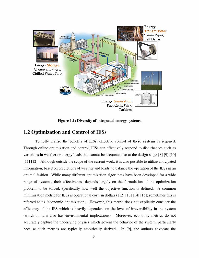
Figure 1.1: Diversity of integrated energy systems. ..................................................................................... 3

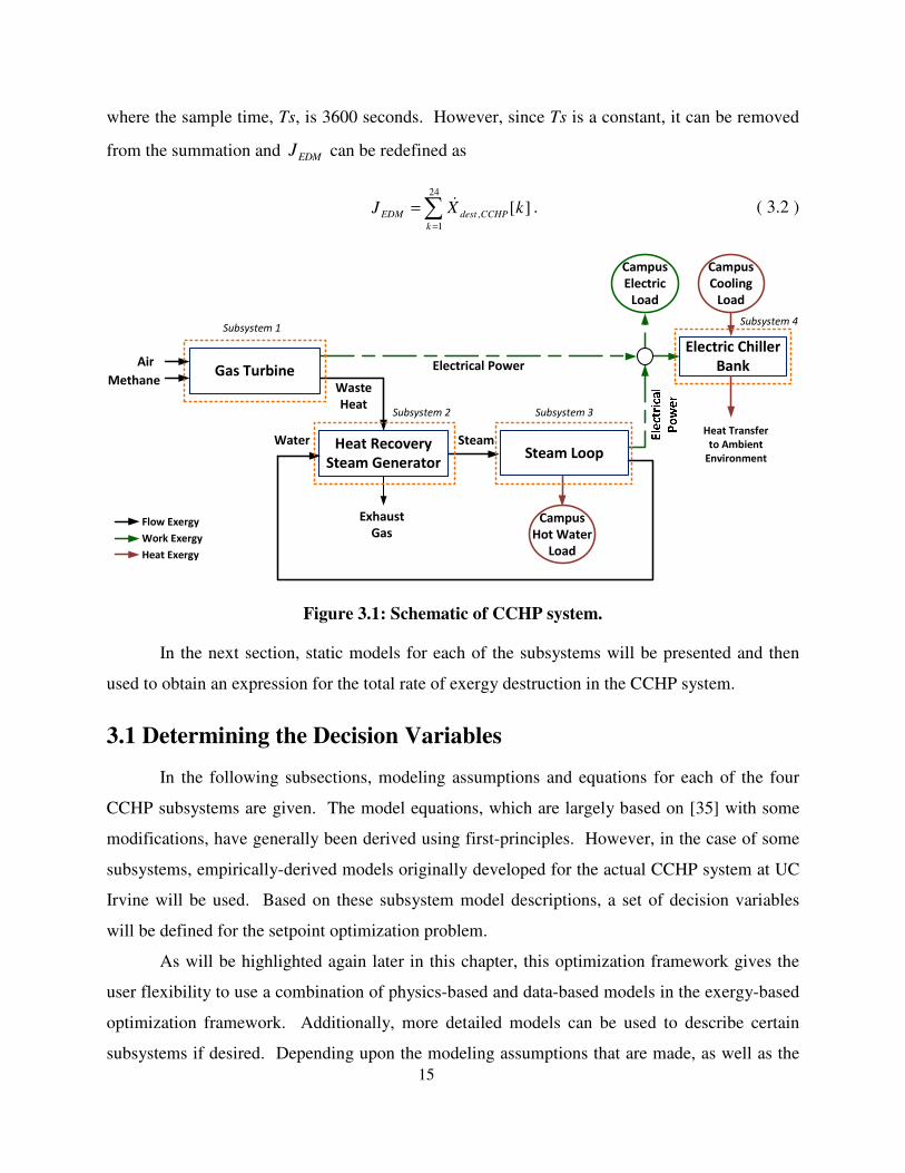
Figure 3.1: Schematic of CCHP system. ..................................................................................................... 15

Figure 3.2: CCHP system schematic highlighting decision variables. ....................................................... 23

Figure 3.3: Ambient temperature profile over 24-hour prediction horizon. ............................................... 24

Figure 3.4: Performance constraints defined over 24-hour prediction horizon. ......................................... 27

Figure 3.5: Optimal setpoints for ẆGT, ṁf, and 1

sf . ................................................................................... 29

Figure 3.6: Optimal setpoints for water mass flow rate, ṁCHW,i , i={1,2,…,7}, through each chiller. ........ 29

Figure 3.7: Optimal setpoints for supply water temperature, TCHWS,i , i={1,2,…,7}, exiting each chiller. 30

Figure 3.8: Optimal setpoints for ẆGT , ṁf , and 1

sf . Also pictured is the total power consumed by the

electric chiller bank (lower right). ...................................................................................................... 34


sf as produced by EDM and energy consumption

minimization in Case 1. Also pictured is the total power consumed by the electric chiller bank

(lower right) computed using the optimal solution of each optimization problem. Circle markers

indicate that the two curves lie directly on top of one another ........................................................... 36

Figure 3.10: Optimal setpoints for ṁCHW,i and TCHWS,i , i={1,2,…,7}, using EDM in Case 1. ..................... 36

Figure 3.11: Optimal setpoints for ṁCHW,i and TCHWS,i , i={1,2,…,7}, using energy consumption

minimization in Case 1. ...................................................................................................................... 37


sf as produced by EDM and energy consumption

minimization in Case 2. Also pictured is the total power consumed by the electric chiller bank

(lower right) computed using the optimal solution of each optimization problem. Circle markers

indicate that the two curves lie directly on top of one another. .......................................................... 38

Figure 3.13: Optimal setpoints for ṁCHW,i and TCHWS,i , i={1,2,…,7}, using EDM in Case 2. ..................... 39

Figure 3.14: Optimal setpoints for ṁCHW,i and TCHWS,i , i={1,2,…,7}, using energy consumption

minimization in Case 2. ...................................................................................................................... 39

xiii

Figure 4.1: Schematic of a standard VCC system....................................................................................... 42

Figure 4.2: Temperature-entropy (T-s) diagram of the Carnot refrigeration cycle. .................................... 43

Figure 4.3: Pressure-enthalpy (P-h) diagram of a standard vapor-compression cycle. .............................. 43

Figure 4.4: Thermal resistance circuit used to estimate overall heat transfer coefficients for the evaporator

and condenser. .................................................................................................................................... 49

Figure 4.5: Schematic of feedforward plus feedback optimization and control architecture. ..................... 53

Figure 4.6: Cooling capacity load profile. .................................................................................................. 53

Figure 4.7: Schematic of experimental system. .......................................................................................... 54

Figure 4.8: Cooling capacity achieved on experimental system. ................................................................ 57

Figure 4.9: Optimized variables plotted as a function of time. ................................................................... 58

Figure 4.10: Control inputs plotted as a function of time. .......................................................................... 58

Figure 4.11: EEV control signal and evaporator superheat plotted as a function of time for ωk = 2000 rpm.

............................................................................................................................................................ 61

Figure 5.1: Schematic depicting control volumes drawn inside each component of the VCC system. Each

control volume contains only the refrigerant flowing through that component. ................................ 66

Figure 5.2: Individual control volumes drawn around each fluid region in an evaporator. ........................ 69

Figure 5.3: Individual control volumes drawn around each fluid region in a condenser. ........................... 71

Figure 5.4: Cooling capacity reference trajectory. ...................................................................................... 84

Figure 5.5: Optimal control input signals,

*uEDM

. ....................................................................................... 85

Figure 5.6: Simulated exergy destruction rate and exergetic efficiency using *uEDM

using the linearized

system model. ..................................................................................................................................... 86

Figure 5.7: Comparison of simulated cooling capacity using the linearized system model with simulated

cooling capacity using nonlinear system model. ................................................................................ 87

Figure 5.8: Comparison of cooling capacity tracking performance using *uEDM

and *uPM

. ....................... 89

Figure 5.9: Closer view of Figure 5.8. ........................................................................................................ 89

Figure 5.10: Comparison between *uEDM

and *uPM

. ................................................................................... 90

Figure 5.11: Comparison of exergy destruction rate, energy consumption rate, and reversible power over

200 second time horizon using *uEDM

and *uPM

. The same range is used for each plot. .................. 91

Figure 5.12: Exergy destruction rate comparison by VCC system component for *uEDM

and *uPM

. The

same range is used for each plot. ........................................................................................................ 93

xiv

Figure 5.13: Instantaneous COP and exergetic efficiency resulting from operating the system with *uEDM

and *uPM

. ............................................................................................................................................ 95

Figure A.1: Flow coefficient map for an EEV. Black points represent experimental data used for map

generation. ........................................................................................................................................ 107

Figure A.2: Volumetric efficiency map for a semi-hermetic reciprocating compressor. Black points

represent experimental data used for map generation. ..................................................................... 107

Figure B.1: Validation of identified model; y1 = 0.5(P1 + P2) and y2 = P2 – P1. ....................................... 109

Figure B.2: Cross validation of the identified model. ............................................................................... 110

Figure C.1: Model validation perturbation signals. .................................................................................. 119

Figure C.2: Linearized model validation of Pc and Pe. ............................................................................. 119

Figure C.3: Linearized model validation of ζe1, eγ , and he2. .................................................................... 120

Figure C.4: Linearized model validation of Tw,e1 and Tw,e2. ...................................................................... 120

Figure C.5: Linearized model validation of ζc1, ζc2, and cγ . ...................................................................... 121

Figure C.6: Linearized model validation of hc1 and hc3............................................................................. 121

Figure C.7: Linearized model validation of Tw,c1, Tw,c2, and Tw,c3. ............................................................ 122

Figure D.1: Comparison of evaporator model states ζe1, Pe, and he2 simulated using the linearized system

model versus using the nonlinear system model for *

EDM=u u . ...................................................... 124

Figure D.2: Comparison of evaporator model states Tw,e1 , Tw,e2 , and eγ simulated using the linearized

system model versus using the nonlinear system model for *

EDM=u u . .......................................... 125

Figure D.3: Comparison of condenser model states ζc1, ζc2, and Pc simulated using the linearized system


EDM=u u . ...................................................... 126

Figure D.4: Comparison of condenser model states hc1, hc3, and cγ simulated using the linearized system


EDM=u u . ...................................................... 127

Figure D.5: Comparison of evaporator model states Tw,c1 , Tw,c2 , and Tw,c3 simulated using the linearized

system model versus using the nonlinear system model for *

EDM=u u . .......................................... 128

xv

List of Symbols

A area m2

a aperture % of maximum

C cooling capacity kW

cp specific heat capacity (at constant pressure) kJ·(kg·K)-1

d disturbance vector --

E energy kJ

F fraction of dimensionless

h specific enthalpy kJ·kg-1

J objective function --

k conductivity kW·(m· K)-1

L length m

m mass kg

mɺ mass flow rate kg·s-1

P pressure kPa

Qɺ heat transfer rate kW

S entropy kJ·K-1

s specific entropy kJ·(kg·K)-1

T temperature K

t time s

u control input --

u control input vector --

UA overall heat transfer coefficient kJ·(s·K)-1

V volume m3

xvi

v velocity m·s-1

v vector of decision variables for setpoint optimization --

Wɺ work transfer rate (i.e. power) kW

X exergy kJ

Xɺ exergy transfer rate kW

x mean quality dimensionless

x dynamic state vector --

α heat transfer coefficient kW·(m2· K)

-1

γ mean void fraction dimensionless

ε HX effectiveness dimensionless

ζ normalized zone length dimensionless

η efficiency dimensionless

ρ density kg·m-3

ψ specific flow exergy kJ·kg-1

ω rotational speed rpm

xvii

List of Subscripts

a air

ach achieved

c condenser (in VCC system)

C cooling demand

c1 superheated fluid region in condenser

c2 two-phase fluid region in condenser

c3 subcooled fluid region in condenser

CHW chiller

CHWR chiller return

CHWS chiller supply

comb combustor (inside gas turbine)

comp air compressor (inside gas turbine)

comp,ref refrigerant compressor in electric chiller

cond condenser (in steam loop)

CR cross-sectional

cv control volume

DAE deaerator

des desired

dest destroyed

e evaporator

e1 two-phase fluid region in evaporator

e2 superheated fluid region in evaporator

f fuel, fan

xviii

g exhaust gas, saturated vapor

g,exhaust exhaust gas exiting HRSG

gen generated

GT gas turbine

H heating demand (in CCHP system), high temperature reservoir

HWR hot water return line

i in (inlet)

k compressor (in VCC system)

L low temperature reservoir

l saturated liquid

o outlet

p pump

p prediction

r,R refrigerant

rev reversible

s steam

sat saturated

SL steam loop

ST steam turbine

turb turbine (inside gas turbine)

u control

v EEV

w water, tube wall

FF feedforward

y output

0 reference environment

12 between the first and second fluid regions (of a heat exchanger)

23 between the second and third fluid regions (of a heat exchanger)

xix

List of Abbreviations

CCHP combined cooling, heating, and power

CHP combined heat and power

COP coefficient of performance

CRC Carnot refrigeration cycle

DOF degree of freedom

EDM exergy destruction minimization

EEV electronic expansion valve

HRSG heat recovery steam generator

HVAC heating, ventilation, and air-conditioning

IC internal combustion

IES integrated energy system

TEV thermostatic expansion valve

VCC vapor-compression cycle

1

Chapter 1

Introduction

This thesis investigates the use of exergy destruction as a minimization metric in the

optimization and control of integrated energy systems (IESs). More broadly, this thesis seeks to

define a systematic methodology for developing objective functions for a wide class of energy

systems that is versatile enough to accommodate the growing diversity of IESs. In addition, the

proposed methodology offers some potential advantages, based on designer tradeoffs, over

current approaches. Section 1.1 provides a general overview of the class of IESs, and Section

1.2 describes the current state of optimization and control of these systems. The latter will be

used to identify specific characteristics needed in an optimization framework in order for it to be

suitable for most IESs.

In this thesis, an emphasis is specifically placed on the operation of IESs as opposed to

the design of these systems. As electrification of energy systems continues to increase, the need

for model-based optimal control strategies for these systems will grow. The approach taken here

is to understand and utilize tools from the thermodynamics community in conjunction with

existing control methodologies to develop a suitable framework. Accordingly, thermodynamic

fundamentals will be discussed in detail in Chapter 2 to familiarize the reader before these ideas

are used in the context of setpoint optimization and control later in the thesis.

1.1 Integrated Energy Systems

Integrated energy systems (IESs) combine prime-mover technologies, such as internal

combustion (IC) engines, and/or fuel cells, with other technologies which directly utilize the

power produced by the prime-mover and/or utilize the thermal energy otherwise wasted in the

production of power. IESs can be thought of as complex systems comprised of many

2

interconnected heterogeneous subsystems such as the prime-movers listed above, thermally-

activated heating systems, desiccant dehumidifiers, vapor-compression refrigeration systems,

and/or energy storage systems [1]. One of the most common types of IESs are combined heat

and power (CHP) systems in which waste heat generated as a byproduct of power generation,

typically with a gas turbine, is then used to provide heating to buildings and/or for other end

uses. Another example is an electric-hybrid automobile wherein an internal combustion engine

generates mechanical power to move the vehicle and simultaneously power the HVAC (heating,

ventilation, and air-conditioning) system on board while storing excess energy as chemical

energy in a battery. IESs are becoming more prevalent because of their environmental,

reliability, economic, and efficiency benefits [1] [2] [3]. A number of government initiatives,

including the Combined Heat and Power Partnership, have been created to improve the CHP

capacity of the U.S. [2]. In 2012 an executive order was signed by President Barack Obama

setting “a national goal of 40GW of new CHP installation” in the U.S. by 2020 [4]. Along with

the increase in installed capacity, it will be critical that the new capabilities are utilized in the

most effective manner possible where the term 'effective' will depend on the end goal of the

system operator.

A key feature of the IES heterogeneity is that it typically spans multiple energy domains -

chemical, electrical, mechanical and thermal - as evidenced by the examples of subsystems

which comprise IESs. Figure 1.1 visualizes this diversity by highlighting how energy

generation, transmission, and consumption/storage can be realized with different forms of

energy. For example, rather than a gas turbine being utilized as the prime mover, a photovoltaic

solar array or fuel cell, or combination thereof, might be used instead as the primary power

generation technology [5]. Moreover, energy storage technologies, such as chilled water tanks or

advanced batteries, are also being used to further improve the efficiency of IESs [6].

The diversity of IESs is also seen in their performance capacity. CHP systems are often

built at a large scale to support energy-intensive manufacturing facilities and for large districts of

buildings, such as college campuses and hospitals [5] [7]. However, similar types of systems are

being developed at a smaller scale for the residential building sector [6]. In summary, the class

of IESs is not only hugely diverse with respect to type of system and scale, but we expect to see

this class of systems continue to grow in the future.

3

Figure 1.1: Diversity of integrated energy systems.

1.2 Optimization and Control of IESs

To fully realize the benefits of IESs, effective control of these systems is required.

Through online optimization and control, IESs can effectively respond to disturbances such as

variations in weather or energy loads that cannot be accounted for at the design stage [8] [9] [10]

[11] [12]. Although outside the scope of the current work, it is also possible to utilize anticipated

information, based on predictions of weather and loads, to balance the operation of the IESs in an

optimal fashion. While many different optimization algorithms have been developed for a wide

range of systems, their effectiveness depends largely on the formulation of the optimization

problem to be solved, specifically how well the objective function is defined. A common

minimization metric for IESs is operational cost (in dollars) [12] [13] [14] [15]; sometimes this is

referred to as ‘economic optimization’. However, this metric does not explicitly consider the

efficiency of the IES which is heavily dependent on the level of irreversibility in the system

(which in turn also has environmental implications). Moreover, economic metrics do not

accurately capture the underlying physics which govern the behavior of the system, particularly

because such metrics are typically empirically derived. In [9], the authors advocate the

4

consideration of different minimization metrics, but the proposed objective functions for energy

and CO2 emissions are empirically-based modifications of an objective function again based on

electricity and fuel costs. In [8] an objective function is proposed which minimizes the daily

operation cost of a micro combined heat and power (µCHP) system and is generalizable for

various systems within the class of µCHP systems. However, the optimization variables are only

the electrical and thermal inputs/outputs of various subsystems such as the energy input to a

thermal storage device; the operation of the thermal storage device itself is not optimized with

respect to the amount of thermal energy it must store.

What is lacking among these examples is an objective function that is physics-based,

generalizable, and modular. Let us describe these attributes in greater detail.

1. Physics-based. As mentioned in the previous section, commonly used minimization

metrics are typically empirically derived. There are two major disadvantages to this approach.

First, these metrics do not necessarily capture the underlying physics of the IES subsystems

which may result in missed opportunities to further improve efficiency (and/or other objectives)

when such metrics are minimized. Secondly, empirically derived metrics cannot easily be

extrapolated if or when a system changes, thereby making them less modular. A physics-based

metric has the potential to overcome these disadvantages.

2. Generalizable. IESs are often comprised of a diverse set of subsystems arranged in

different architectures or configurations and therefore, generalizability in the methodology for

designing an appropriate objective function is necessary [1] [8]. Unfortunately, a major

challenge in accomplishing this comes from the fact that the individual subsystems which

comprise IESs are heterogeneous and typically characterized using different efficiency metrics.

For example, internal combustion engines are often characterized in terms of their fuel efficiency

whereas heat and cooling systems are typically characterized in terms of coefficient of

performance (COP). It is difficult to combine these metrics in a meaningful way that preserves

the physics of the system.

3. Modular. In addition to having a metric that is generalizable to different types of

systems, it may be desirable to quickly modify an objective function to include or exclude

5

specific subsystems in a particular IES. Therefore, an objective function which can be easily

modified for different systems in a systematic way is desirable.

The scope of this thesis is to develop a systematic methodology for deriving objective

functions to be used in conjunction with optimization and optimal control algorithms for

improving operational efficiency and performance of IESs. In the following chapters, a

thermodynamics-based minimization metric, exergy destruction, will be described and

formulated as the foundation for deriving appropriate objective functions. The exergy

destruction minimization (EDM) objective will be constructed as the sum of the exergy

destruction in each subsystem of the IES. This will provide a common and modular metric for

evaluating the efficiency of the complete system since exergy destruction can be used to

characterize irreversibilities across multiple energy domains (chemical, electrical, mechanical,

thermal). The merits of the framework will be demonstrated through various case studies.

1.3 Organization of Thesis

The thesis is organized as follows. Chapter 2 introduces the concept of exergy and

outlines the exergy-based optimization framework. In Chapter 3, the generalizability and

modularity of the optimization framework is demonstrated through static setpoint optimization of

a combined heating, cooling, and power (CCHP) system with varying performance demands

over a 24-hour period. Moreover, the benefits of the physics-based metric are highlighted in a

comparison between EDM and conventional energy minimization of the CCHP system. In

Chapters 4 and 5, the EDM framework is applied to an individual energy system, specifically a

vapor-compression cycle (VCC) system. Here the emphasis is extended beyond setpoint

optimization to include control of the physical system itself for setpoint regulation. In Chapter 4,

a static setpoint optimization of a VCC system conducted using EDM is augmented with a

feedforward plus feedback control framework designed to operate the system at the optimal

operation setpoints. Experimental results are provided to validate the approach. In Chapter 5,

the dynamic rate of exergy destruction is derived for the VCC system so that transient, rather

than steady-state, operation of the system can be considered. A finite-horizon optimal control

problem is then formulated and solved offline to yield the optimal control input sequences for

tracking a desired cooling capacity profile. The results are validated on a nonlinear simulation

6

model. Again, the benefits of the EDM metric, now in the context of transient operation, are

highlighted in a comparison between EDM and energy consumption minimization of the VCC

system. The thesis concludes in Chapter 6 with a summary of research contributions as well as

directions for future work.

7

Chapter 2

Exergy-Based Optimization Framework

2.1 Thermodynamic Fundamentals

The first law of thermodynamics is a statement of energy conservation. That is to say,

energy can never be destroyed. The second law introduces the notion of entropy and connects it

to the irreversibility that is observed in natural phenomena by postulating that a process can only

proceed in “the direction that causes the total entropy of the system plus surroundings to

increase” [16]. It distinguishes between spontaneously feasible and infeasible processes.

It is the combination of the first and second laws of thermodynamics that is particularly

powerful. Exergy (also referred to as “availability”) is defined as the maximum reversible work

that can be extracted from a substance at a given state during its interaction with a given

environment. Thermomechanical exergy is defined mathematically as

0

cv cv cvdX dE dS

Tdt dt dt

= − ( 2.1 )

where

2 2

2 2

cv ii i i

i o

oo o o

dEQ W m h gz m h gz

dt

v v = − + + + − + +

∑ ∑ɺ ɺ ɺ ɺ ( 2.2 )

and

jcv

i i gen

i o

o

j

o

j

QdSm s m s S

dt T= + − +∑ ∑ ∑

ɺɺɺ ɺ . ( 2.3 )

8

In both the energy and entropy rate balances, i denotes inlets and o denotes outlets. In Eq. 2.3,

jQɺ is the heat transfer rate at the location on the control volume boundary where the

instantaneous temperature is Tj.

Whereas energy is always conserved, exergy is not. Similarly to energy, exergy can be

transferred in three ways: by heat transfer, work, or through mass exchange with the

environment. However, contrary to energy, exergy is destroyed during irreversible phenomena

such as chemical reactions, mixing, and viscous dissipation. The amount of exergy destroyed in a

system or through a process is a measure of the loss of potential to do work and is proportional to

the amount of entropy generated in the system; this is described by the Gouy-Stodola theorem

[17]:

0 0dest genX ST= ≥ɺɺ . ( 2.4 )

Therefore, exergy destruction is a useful quantity to consider when characterizing the efficiency

of thermodynamic systems. Specifically, the exergetic (second-law) efficiency, IIη , is defined as

[18]

Exergy destroyed

1Exergy supplied

IIη = − . ( 2.5 )

The total exergy rate balance for a control volume is given by

00

exergy transfer exergy transfer accompanyingexergy transfer accompanying mass taccompanying work transferheat transfer

1cv cj cv i i

j

o o

i oj

vdX T dVQ W P m m

dt T dtψ ψ

= − − − + −

∑ ∑ ∑ɺ ɺ ɺ ɺ

��

ransfer

destX−

��

ɺ

��

( 2.6 )

where the specific flow exergy, ψ, is defined as

( ) ( )2

ch

0 0 02

h h T s s gzv

ψ ψ= − − + ++− . ( 2.7 )

The quantities T0, P0, h0, and s0 are the temperature, pressure, specific enthalpy, and specific

entropy, respectively, of the reference environment. The reference environment is typically

chosen as an infinite reservoir with which the system is interacting, such as the ambient

9

environment. The use of a reference environment for defining exergy is consistent with the way

in which all forms of potential energy are defined.

In addition to characterizing thermal and mechanical potential, exergy can also

characterize chemical potential. This is represented by the term chψ in Eq. 2.7 which is the

chemical contribution to the total specific flow of exergy entering and leaving a control volume.

For example, in the case of combustion, the chemical exergy is the maximum reversible work

that can be extracted through the reaction of the fuel with environmental components [16].

2.2 Exergy-Based Analysis and Optimization

2.2.1 Exergy Analysis

Like the first and second laws of thermodynamics, exergy can be used to analyze systems

and understand their behavior. Exergy analysis has been used extensively in the

thermodynamics community to understand which subsystems and/or components are responsible

for the greatest irreversibilities in the overall system, thereby influencing design changes at the

system and/or component level [19]. In the context of individual thermal systems, [20] provides

an extensive review of exergy analyses that have been conducted on vapor-compression cycle

(VCC) systems, particularly highlighting the effect of different refrigerants, as well as key

parameters such as evaporating temperature, on the exergetic efficiency of the system. More

recently, [21] uses exergy analysis to evaluate the better of two designs of expander cycles used

in a refrigeration system. For integrated energy systems (IESs), [22] analyzes each component in

a combined-cycle power plant and highlights the heat recovery steam generator as the one with

the lowest exergetic efficiency. It is suggested in [22] that operating parameters be optimized in

order to improve performance.

Exergy analysis has also played a significant role in the area of thermoeconomics, also

called exergoeconomics, which is a methodology for calculating the monetary costs associated

with the design and operation of a thermal system, particularly by assigning monetary costs to

the various exergy flows in a system [23] [24] [25]. More recently, Lazaretto and Tsatsaronis

presented a general approach for evaluating exergy-based efficiencies and costs in thermal

systems [26].

10

2.2.2 Exergy Destruction Minimization

In addition to exergy analysis, researchers have used exergy destruction minimization

(EDM), also known as entropy generation minimization or thermodynamic optimization [27], to

optimize design and operational parameters in many thermal systems [28] [29]. In particular,

design parameters, such as heat exchanger geometry, have been optimized using EDM [30] [31]

[32]. However, while exergy destruction minimization (EDM) has been used to determine

design and nominal operational parameters, to the knowledge of the authors, exergy destruction

minimization (EDM) has not been used as a metric in optimal control of energy systems. We

believe EDM is particularly suitable for the optimization of IESs because of two features of

exergy destruction:

1.) Exergy destruction can be used to characterize irreversible losses across multiple

energy domains. Therefore, exergy destruction provides us with a common metric to

describe the efficiency of different components or subsystems which are typically

defined using different efficiency metrics. Consider an engine-driven VCC system:

internal combustion (IC) engines are often characterized in terms of their fuel

efficiency whereas heating and cooling systems are typically characterized in terms of

coefficient of performance (COP). It is difficult to combine these metrics in a

meaningful way that preserves the physics of the system. Describing the efficiency of

the IC engine and VCC system in terms of exergy destruction would overcome this

hurdle [33].

2.) Total exergy destruction for a given system can simply be expressed as the sum of the

exergy destroyed in its components and/or subsystems. This modularity is

particularly useful when considering complex systems such as IESs because the

objective function can be easily modified to include/exclude individual subsystems as

desired by the engineer.

2.2.3 Relationship Between EDM and Power Minimization

In the context of optimization, it is common for the amount of power consumed

(generated) in a system to be minimized (maximized). The relationship between exergy

destruction rate minimization and power minimization is characterized by the Gouy-Stodola

theorem (Eq. 2.4) which can be equivalently expressed [27] as

11

dest rev

X W W= −ɺ ɺ ɺ . ( 2.8 )

The reversible rate of change of work, rev

Wɺ , also called reversible power, refers to the amount of

power that the system would consume (or produce) if there were no irreversibilities in the

system. Let us define two objective functions, 1J and 2J , where 1J is equal to the rate of

exergy destruction and 2J is equal to the actual power consumed (or produced).

1 dest rev

J X W W== −ɺ ɺ ɺ ( 2.9 )

2

J W= ɺ ( 2.10 )

Equation 2.8 implies that if the quantity rev

Wɺ is constant with respect to the decision variables of

an optimization problem, then the minimizations of 1J and 2J are equivalent [27], i.e.

( ) ( )1 2min minrevW C

J J=

=ɺ

. ( 2.11 )

Examples of when the reversible work/power is, and is not, constant with respect to the decision

variables of an optimization problem will be discussed in Chapter 3. Of particular interest is

when the equivalence between exergy destruction rate minimization and power minimization

does not exist which will be explored throughout this thesis.

2.3 EDM Framework for Integrated Energy Systems

While exergy destruction minimization (EDM) has been used to determine design and

nominal operational parameters, exergy destruction minimization (EDM) has not been used to

optimize IESs over varying load profiles nor in conjunction with optimal controllers such as

model predictive control. In this thesis EDM is applied as an optimization metric in the context

of real-time operation of energy systems.

Optimization of IESs can be characterized by multiple (competing) objectives such as

meeting specified performance demands, maximizing system efficiency, and/or minimizing wear

on physical components. It is necessary to define a mathematical function that captures the

objectives for a given IES and can be minimized or maximized to yield an optimal solution.

In this optimization framework, we will focus on two primary objectives: 1) meet

specified performance demand, and 2) maximize system efficiency. The first objective will be

12

enforced as a constraint. Therefore, we seek an objective function which captures the second

objective of maximizing system efficiency. Given the attributes of exergy destruction

highlighted in Section 2.2.2, exergy destruction is an appropriate physics-based, generalizable,

and modular metric to be used for the optimization of IESs. This optimization framework can be

applied using the following procedure:

1. Define the objective function to minimize the total exergy destroyed over a specified time

horizon. For example:

,

1

[ ·]N

dest total

k

EDMJ X k Ts

=

=∑ ɺ ( 2.12 )

where Ts is the discrete sample time.

2. Determine the decision variables based on modeling assumptions and available degrees

of freedom (DOFs).

3. Derive an expression for the rate of exergy destruction, dest

Xɺ , in each subsystem of the

overall system (or in each component of a single system).

4. Define the total exergy destruction rate for the system by summing together the exergy

destruction rates of each subsystem:

, ,1 ,2 ,dest total subsystem subsystem subsystem nX X X X= + + +ɺ ɺ ɺ ɺ⋯ . ( 2.13 )

5. Define constraints for the optimization problem.

This procedure is intentionally generalized to highlight the modularity of this approach.

Noteworthy is the fact that it is not necessary to introduce constant weights on the individual

subsystem rates of exergy destruction in Eq. 2.13 because in this objective function, the same

quantity (exergy destruction rate in units of power) is being summed for every subsystem.

Therefore, if one individual subsystem destroys more exergy than others, it will inherently be

penalized more than the other subsystems in the optimization. This highlights a major advantage

of this approach since tuning weightings in an objective function comprised of terms in different

units would become increasingly difficult as the complexity of the system increases.

13

In the next chapter, the optimization framework outlined here will be applied to a

combined cooling, heating, and power (CCHP) system for the purpose of setpoint optimization.

When the equivalence between exergy destruction rate minimization and power minimization

exists, it will be shown that power and exergy destruction rate can be interchanged in a larger

objective function. When equivalence does not exist, it will be shown that the EDM provides a

solution which destroys less exergy than an energy consumption minimization of the same

system while also favoring those subsystems with higher isentropic efficiencies. In Chapter 5,

this framework will be used with an optimal control algorithm to control a vapor-compression

cycle (VCC) system.

14

Chapter 3

Setpoint Optimization of a CCHP System

A combined cooling, heating, and power (CCHP) system is a common type of integrated

energy system (IES). In this chapter the exergy destruction minimization (EDM) framework

outlined in Chapter 2 is applied to a CCHP system. The results will highlight the modularity of

the EDM framework in describing irreversibilities across multiple energy domains. In particular,

the notion of interchangeability will be introduced wherein exergy destruction rate and power

consumption can be interchanged for particular subsystems in the overall objective function to

yield the same solution as in EDM. Finally, the advantages of EDM as compared to energy

consumption minimization will be explored.

The CCHP system considered in this chapter is shown schematically in Figure 3.1 and is

modeled after an existing system at the University of California, Irvine [34]. It is comprised of

four major subsystems: a gas turbine, a heat recovery steam generator (HRSG), a steam loop, and

an electric chiller bank. The goal of this case study is to find the optimal operation setpoints for

the CCHP system at each hour for 24 hours of operation. The problem will be posed as a static

optimization problem, and the system will be described using static models of the four

subsystems. The decision variables in the optimization problem will be chosen as independent

operational parameters for which setpoint values can be assigned. Based on the optimization

framework outlined in Chapter 2, the objective function for minimizing exergy destruction,

EDMJ , is defined as

24

,

1

[ ]·dest CCHP

k

EDM Tk sJ X=

=∑ ɺ ( 3.1 )

15

where the sample time, Ts, is 3600 seconds. However, since Ts is a constant, it can be removed

from the summation and EDMJ can be redefined as

24

,

1

[ ]dest CE M CHPD

k

J X k=

=∑ ɺ . ( 3.2 )

Figure 3.1: Schematic of CCHP system.

In the next section, static models for each of the subsystems will be presented and then

used to obtain an expression for the total rate of exergy destruction in the CCHP system.

3.1 Determining the Decision Variables

In the following subsections, modeling assumptions and equations for each of the four

CCHP subsystems are given. The model equations, which are largely based on [35] with some

modifications, have generally been derived using first-principles. However, in the case of some

subsystems, empirically-derived models originally developed for the actual CCHP system at UC

Irvine will be used. Based on these subsystem model descriptions, a set of decision variables

will be defined for the setpoint optimization problem.

As will be highlighted again later in this chapter, this optimization framework gives the

user flexibility to use a combination of physics-based and data-based models in the exergy-based

optimization framework. Additionally, more detailed models can be used to describe certain

subsystems if desired. Depending upon the modeling assumptions that are made, as well as the

Gas Turbine Electrical PowerMethane

Waste

Heat

Air

Flow Exergy

Work Exergy

Heat Exergy

Heat Recovery

Steam Generator

Exhaust

Gas

SteamWaterSteam Loop

Campus

Hot Water

Load

Campus

Electric

Load

Electric Chiller

Bank

Heat Transfer

to Ambient

Environment

Campus

Cooling

Load

Subsystem 1Subsystem 4

Subsystem 3Subsystem 2

16

actuation capability of the actual system under consideration, different decision variables will be

available for optimization.

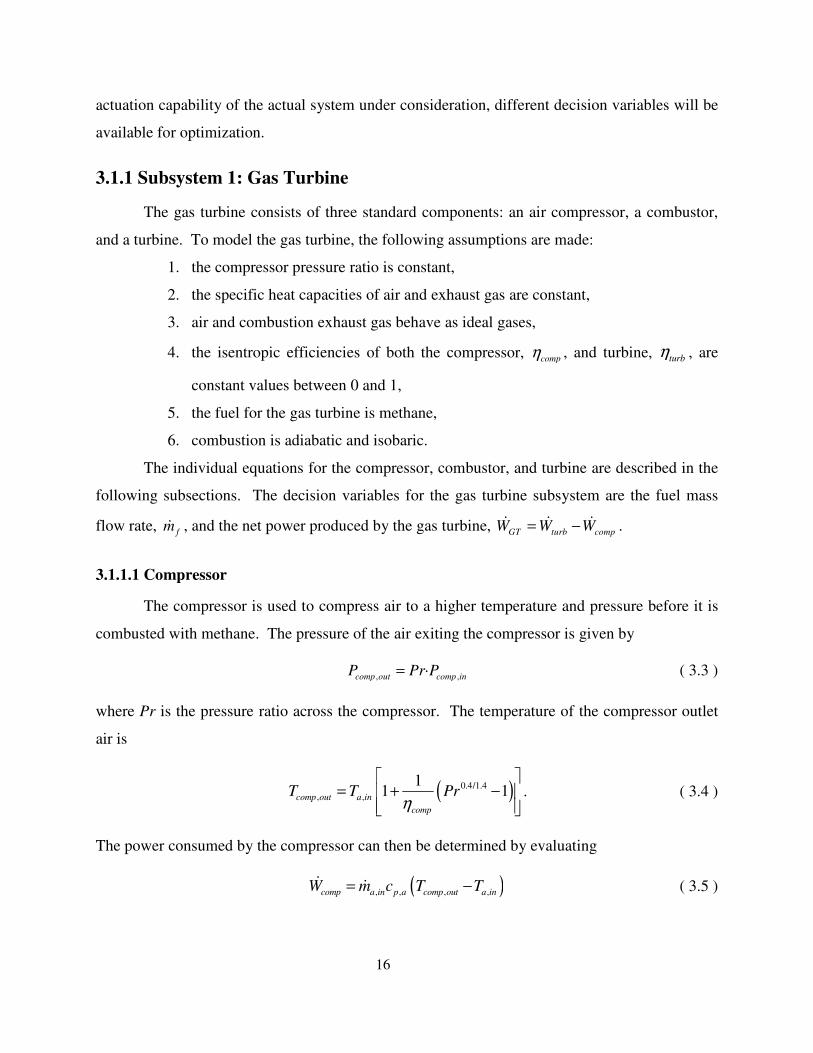
3.1.1 Subsystem 1: Gas Turbine

The gas turbine consists of three standard components: an air compressor, a combustor,

and a turbine. To model the gas turbine, the following assumptions are made:

1. the compressor pressure ratio is constant,

2. the specific heat capacities of air and exhaust gas are constant,

3. air and combustion exhaust gas behave as ideal gases,

4. the isentropic efficiencies of both the compressor, comp

η , and turbine, turbη , are

constant values between 0 and 1,

5. the fuel for the gas turbine is methane,

6. combustion is adiabatic and isobaric.

The individual equations for the compressor, combustor, and turbine are described in the

following subsections. The decision variables for the gas turbine subsystem are the fuel mass

flow rate, f

mɺ , and the net power produced by the gas turbine, GT turb comp

W W W−=ɺ ɺ ɺ .

3.1.1.1 Compressor

The compressor is used to compress air to a higher temperature and pressure before it is

combusted with methane. The pressure of the air exiting the compressor is given by

, ,

·comp out comp in

Pr PP = ( 3.3 )

where Pr is the pressure ratio across the compressor. The temperature of the compressor outlet

air is

( )0.4/1.4

, ,

11 1comp out a in

comp

T T Prη

= + −

. ( 3.4 )

The power consumed by the compressor can then be determined by evaluating

( ), , , ,comp a in p a comp out a inW m c T T= −ɺ ɺ ( 3.5 )

17

where it is assumed that ηcomp, the isentropic efficiency of the compressor, is a constant value

between 0 and 1 and is specified in the optimization problem.

3.1.1.2 Combustor

The stoichiometric chemical reaction between methane (CH4) and the compressed air

which takes place in the combustor is described by

4 2 2 2 2 20.5CH 3.76N O 0.5CO H O 3.76N+ + → + + . ( 3.6 )

However, in actuality, the combustion reaction in gas turbines is typically characterized by an

equivalence ratio less than one, where [16] defines the equivalence ratio as

( )

( )actual

stoichiometric

FA

FAφ = . ( 3.7 )

Here we assume an air-fuel ratio of 22.0, which is characterized by the following chemical

reaction:

4 2 2 2 2 2 20.5CH 4.82N 1.2826O 0.5CO H O 4.82 0.28 6N 2 O+ + → + + + . ( 3.8 )

Based on Eq. 3.8, the mass flow rates of fuel (methane), air, and combustion products are related

to one another as shown in Eq. 3.9 and Eq. 3.10.

,

1.02g a in

m m=ɺ ɺ ( 3.9 )

,22.0

a in

f

m

m=

ɺ

ɺ ( 3.10 )

The temperature of the combustion products leaving the combustor can be obtained by

evaluating the following energy balance:

4, CH ,

, ,

LHVf

comb out comp out

a in p a

Tc

mT

m= +

ɺ

ɺ ( 3.11 )

where 4CHLHV is the lower heating value of methane [16]. The combustion process is assumed

to be isobaric so that , ,comb out comb inP P= .

18

3.1.1.3 Turbine

After exiting the combustor, the combustion products, modeled as an ideal gas, enter the

turbine. The temperature of the exhaust gas as it leaves the turbine is given by

0.4/1.4

,

, ,

,

1 1turb out

turb out comb out turb

comb out

PT T

Pη

= − −

( 3.12 )

where ηturb, the isentropic efficiency of the turbine, is a constant between 0 and 1 and is specified

in the optimization problem. The power produced by the turbine is then evaluated using the

equation

( ), , ,turb g p a out comb turb outW m c T T= −ɺ ɺ . ( 3.13 )

3.1.2 Subsystem 2: Heat Recovery Steam Generator

The heat recovery steam generator (HRSG) is used to generate steam from the exhaust

gas exiting the gas turbine. For simplicity, it is modeled here as a counter-flow heat exchanger

although in general, it contains many individual components such as boilers and an economizer.

The effect of the unmodeled components is captured using a lumped heat exchanger

effectiveness, ε, which is taken to be constant in the optimization problem. However, with more

detailed models, the effectiveness could be expressed in terms of operational parameters thereby

creating an additional optimization degree of freedom (DOF). To model the HRSG, the

following assumptions are made:

1. the HRSG can be modeled as a counter-flow heat exchanger with constant

effectiveness, ε,

2. the pressure in the water/steam mass stream drops by a constant factor, ,

HRSG

p wf ,

between the inlet and outlet of the HRSG,

3. the specific heat capacities of water and exhaust gas are assumed to be constant,

4. the mass flow rate of the steam exiting the HRSG is equal to the mass flow rate of

water entering the HRSG: w sm m=ɺ ɺ .

There are no decision variables specifically associated with the HRSG; once ṁf and ẆGT have

been determined for Subsystem 1, Eqs. 3.14 – 3.17 can be evaluated.

Based on Assumption 2, the pressure of the steam exiting the HRSG is

19

, , ,

HRSG

w out p w w inP f P= ( 3.14 )

where ,

HRSG

p wf is the pressure loss factor in the water/steam mass stream, and Pw,in is specified as a

constant in the optimization problem. The heat exchanger effectiveness is described by

( ), , , ,g in g out g in w inT T T T− = −ε ( 3.15 )

where Tw,in and ε are specified as constants in the optimization problem. In order to compute the

temperature at which steam exits the HRSG, the following energy balance is first used to find the

enthalpy at which the steam exits the HRSG:

( ) ( ), , , , ,g p g g in g out w s out w inm c T T hm h− = −ɺ ɺ . ( 3.16 )

Then the approximated linear relationship, shown in Eq. 3.17, between superheated water vapor

enthalpy and temperature is used to determine Ts,out.

, ,1 , ,2s out h s out h

hT θ θ= + ( 3.17 )

Equation 3.16 assumes that there is enough potential in the exhaust gas to generate steam. The

numerical values for the regression coefficients, ,1h

θ and ,2h

θ , are provided in Table 3.1 and were

obtained using fluid property tables provided in [36].

Table 3.1 Linear Regression Coefficients for Ts,out

Coefficient Value

,1hθ 0.4445

,2hθ 1314.75

3.1.3 Subsystem 3: Steam Loop

The steam generated in the HRSG is used for two purposes upon entering the steam loop:

generating electricity via a steam turbine and meeting the campus hot water demand. To model

the steam loop, the following assumptions are made:

1. there is no leakage of water/steam anywhere in the steam loop,

2. the deaerator and condenser are regulated at specified constant pressures, PDAE

and Pcond,1, respectively,

3. steam behaves like an ideal gas

20

4. in the range of operation under consideration, the specific heat capacity of steam,

cp,s, varies linearly with temperature,

5. in the range of operation under consideration, the saturation temperature of water,

Tw,sat, is linearly dependent on the inlet water pressure, Pw,out,

6. steam is in a gaseous state upon exiting the steam turbine

7. steam is in a gaseous state upon exiting the heat exchanger with the hot water

circuit

8. the isentropic efficiency of the steam turbine, STη , is a constant between 0 and 1,

9. and the water pumps have 100% mechanical efficiency.

The inlet steam mass flow rate, ,s inmɺ , is divided into two mass flow rates, determined by

1

sf , the fraction of steam diverted towards the steam turbine:

,1 1 , ,s

s s inm f m=ɺ ɺ ( 3.18 )

( ),2 1 ,1 .s

s s inm f m= −ɺ ɺ ( 3.19 )

The electrical power generated by the steam turbine is then evaluated using the expression

0.25

,1

,1 , ,

,

1cond

ST s p s ST s in

s in

PW m c T

Pη

= −

ɺ ɺ ( 3.20 )

where a linear relationship between Ts,in and cp,s is approximated as shown in Eq. 3.21. The

numerical values for ,1cpθ and ,2cp

θ are provided in Table 3.2.

, ,1 , ,2p s cp s in cp

Tc θ θ= + ( 3.21 )

Table 3.2 Linear Regression Coefficients for cp,s

Coefficient Value

,1cpθ 0.0006

,2cpθ 1.6599

21

The remaining steam is used to meet the campus hot water demand by exchanging

thermal energy with the campus hot water circuit. The amount of heat delivered to the hot water

return line is

( ), , ,H s p s s in w satQ m c T T= −ɺ ɺ ( 3.22 )

where the saturated water temperature, Tw,sat, is evaluated at the pressure of the steam as it

exchanges heat with the hot water line, Pw,out, using the approximated linear relationship

, ,1 , ,2w sat T w out T

T Pθ θ= + . ( 3.23 )

The numerical values for the regression coefficients are provided in Table 3.3.

Table 3.3 Linear Regression Coefficients for Tw,sat

Coefficient Value

,1Tθ 0.0249

,2Tθ 435.47

The steam exiting the steam turbine is pumped through the condenser towards the

deaerator. The steam exiting the heat exchanger with the hot water circuit passes through a

second condenser and then the two streams of water combine as they flow through the deaerator

and are pumped back towards the HRSG. The power consumed by each of the pumps is

( ),1

,1 ,1

s

p DAE cond

w

mW P P

ρ= −ɺ

ɺ ( 3.24 )

and

( ),

,2 ,

s in

p w out DAE

w

mW P P

ρ= −ɺ

ɺ . ( 3.25 )

The decision variable associated with the steam loop is 1

sf .

3.1.4 Subsystem 4: Electric Chiller Bank

The electric chiller bank consists of seven individual chillers. Auxiliary equipment such

as cooling towers and pumps are omitted from this analysis. The rate of cooling provided by the

ith chiller is given by

22

( ), , , ,c i CHW i p w CHWR CHWS im c T TQ = −ɺɺ . ( 3.26 )

The chiller water return temperature CHWRT is assumed to be the same for each chiller and is

specified as a constant in the optimization problem. Moreover, cp,w, the specific heat of water, is

a known constant. However, the water mass flow rates, , {1, 2,..., 7 , }CHW i

m i ∈ , and the supply

water temperatures, , {1, 2,..., 7} , CHWS i

T i ∈ , for the individual chillers are not fixed and therefore

are decision variables in the optimization problem.

The power consumed by the ith chiller, ,CHW iWɺ , is described using an empirical model

developed in [34] which is a linear function of the cooling capacity provided by that chiller:

, ,iCHW i c i iW Qα β= +ɺɺ . ( 3.27 )

The regression coefficients α and β for each chiller are given in Table 3.4. Note that Chiller 5 is

the most efficient chiller for variations in cooling capacity. This feature will be highlighted in

the results presented in Section 3.4.

Table 3.4 Linear Regression Parameters for Chiller Power Consumption

α β

Chiller 1 0.1357 204.91

Chiller 2 0.1357 204.91

Chiller 3 0.1716 99.453

Chiller 4 0.1604 686.29

Chiller 5 0.1213 454.94

Chiller 6 0.3683 151.29

Chiller 7 0.3127 427.63

3.1.5 Summary of Decision Variables

There are a total of 17 decision variables to be optimized for the CCHP system. These

are depicted visually in Figure 3.2 to give the reader a better understanding of what the decision

variables are in the context of the overall system.

23

Figure 3.2: CCHP system schematic highlighting decision variables.

3.2 Derivation of the Exergy Destruction Rate

In order to derive an expression for the total rate of exergy destruction (at steady-state) in

the CCHP system, each of the aforementioned subsystems is analyzed individually. The exergy

rate balance for a control volume is given by

001cv cv

j o o dest

j i oj

cv i i

dX T dVQ W P m m X

dt T dtψ ψ

= − − − + − − ∑ ∑ ∑ɺ ɺ ɺɺ ɺ ( 3.28 )

where the flow exergy, ψ , is defined as

( )2

ch

0 0 0 +2

.h h T s s gzv

ψ ψ= − − − + + ( 3.29 )

The exergy rate balance for a control mass (i.e. closed system) is

0 ch

01 .j dest

j j

TdX dVQ W P X

dt T dtX

= − − − + − ∑ ɺ ɺɺɺ ( 3.30 )

The reference state is chosen to be the ambient environment and is described by T0 and P0

where T0 will be specified at each hour and P0 = 101.325 kPa is atmospheric pressure. The

reference temperature is updated at each hour based on a typical 24-hour ambient temperature

profile for summer months [37] in Southern California, shown in Figure 3.3.

, ,,

{1,2,...,7}

CHW i CHWS iT

i

m

∈

ɺ

STWɺ

GTWɺ

fmɺ

24

Figure 3.3: Ambient temperature profile over 24-hour prediction horizon.

3.2.1 Subsystem 1: Gas Turbine

The first control volume is drawn around the gas turbine as shown in Figure 3.1. We

apply Eq. 3.28 to this control volume and make the following simplifications based on the fact

that the gas turbine is operating at steady-state at each hour and there is no heat transfer across

the boundary of the control volume:

cvdX

dt

01 j

j

TQ

T

= −

∑ ɺ

0cv

cv

dVW P

dt− −ɺ i o o dest

i o

im m Xψ ψ

+ − −

∑ ∑ ɺɺ ɺ . ( 3.31 )

The expression for the rate of exergy destruction in the gas turbine is

,

c

,,,

h

,comp f fdest GT turb a i a inn g o out tu gX W m m mW ψ ψ ψ= + + −− ɺɺ ɺ ɺ ɺɺ . ( 3.32 )

Note that the flow exergy of air, , ,a in a inm ψɺ is zero in this analysis because the air enters the

compressor at the reference state.

3.2.2 Subsystem 2:HRSG

The second control volume is drawn around the heat recovery steam generator (HRSG)

as shown in Figure 3.1. Subsystem 2 is assumed to be operating at steady state and there is no

exergy transfer by work or heat across the boundary of the control volume. Therefore, the

expression for the rate of exergy destruction in the HRSG is given by Eq. 3.34.

0 4 8 12 16 20 2410

12

14

16

18

20

22

24

26

28

30

32

Time (hour)

Am

bie

nt T

em

pe

ratu

re (

de

g C

)

25

cvdX

dt

01 j

j

TQ

T

= −

∑ ɺ

cvW− ɺ0

cvdVP

dt− dest

in out

m m Xψ ψ

+ − −

∑ ∑ ɺɺ ɺ ( 3.33 )

( ) ( ), , ,, ,g g in g exhausdest HRSG w sin s ut o twX m m mψ ψ ψ ψ= +− −ɺ ɺ ɺɺ ( 3.34 )

3.2.3 Subsystem 3: Steam Loop

The third control volume is drawn around the steam loop as shown in Figure 3.1.

Subsystem 3 is assumed to be operating at steady-state so the differential terms in Eq. 3.35 are

zero. In this control volume, the exergy transferred from the steam to meet the hot water load is

modeled as H

Qɺ . There is exergy transfer by work due to the power generated by the steam and

the power consumed by the two water pumps. Finally, the steam entering, and the water exiting,

the steam loop contain flow exergy.

cvdX

dt

001 cv

vj

j

c

T dVQ W P

T dt

= − − −

∑ ɺ ɺ

dest

in out

m m Xψ ψ

+ − −

∑ ∑ ɺɺ ɺ ( 3.35 )

The final expression for the rate of exergy destruction in the steam loop is

( ) ( ) ( ), ,1 ,1 ,, 1 p p ST s io

dest SL H s w w o tn u

HWR

W WT

X QT

W m mψ ψ

= − − − − − + −

+ɺ ɺ ɺ ɺ ɺɺɺ . ( 3.36 )

Note that the flow exergy terms in Eq. 3.34 will cancel out with the flow exergy terms in

Eq. 3.36 because they represent a closed circuit of water which circulates through Subsystems 2

and 3 and repeatedly changes phase between steam and water.

3.2.4 Subsystem 4: Electric Chiller Bank

The fourth and final control volume is drawn around the electric chiller bank as shown in

Figure 3.1. Subsystem 4 is assumed to be operating at steady-state. Since there is no mass

transfer across the boundary of the control volume, though, the electric chiller bank can be

treated as a closed system. Therefore, Eq. 3.30 is used to derive the rate of exergy destruction in

the electric chiller bank:

dX

dt

001 j

j

T dVQ W P

T dt

= − − −

∑ ɺ ɺ ch

X

+

ɺdestX− ɺ . ( 3.37 )

26

The rate of exergy destruction for the entire electric chiller bank is given by the summation

7

0, ,

1

, ,1dest CHW C comp ri

i CHWR

ef i

TX Q W

T=

= − +

∑ ɺɺ ɺ . ( 3.38 )

3.2.5 Expression for Total Exergy Destruction Rate

An expression for the total rate of exergy destruction in the complete CCHP system can

be obtained by summing the expressions for dest

Xɺ given in Eqs. 3.32, 3.34, 3.36, and 3.38. After

some cancellations, this yields

( )0,

70

,

1

ch

, ,

,1 ,2 , ,

1

1

comp f f g exhaust g exhaust

p p ST comp re

dest CCHP turb H

HWR

C i

i C R

f i

HW

m m

W

TX W W Q

T

TQ

TW W W

ψ ψ

=

= + − + − −

+ + − + − +

−

∑

ɺɺ ɺ

ɺ ɺ ɺ

ɺ ɺ

ɺ

ɺ

ɺ

( 3.39 )

where ch 51.849fψ = MJ/kg for methane (CH4) at the standard reference state [16] and

( ) , ,

, , , 0 0 ,

0 0

.ln lng exhaust g exhaust

g exhaust p g g exhaust p g g

T PT T T c R

T Pcψ

− − − = ( 3.40 )

The value for ch

fψ varies with temperature, but the variation is sufficiently small that ch

fψ is

often approximated as constant [16]. While Eq. 3.39 is derived using first principles, the

expressions for the individual terms, such as the power produced by the turbine, can be derived

either from first principles or from data. While there are many advantages of using purely

physics-based models, these are not always available. However, by starting with Eq. 3.39 as the

skeleton of the objective function, the overall metric to be minimized is based in fundamental

thermodynamics regardless of whether an empirical or physics-based expression is used to

characterize pump power, etc.

3.3 Defining the Constraints

There are three performance demands for the CCHP system which must be satisfied: an

electricity demand, a hot water demand, and a cooling demand. The cooling and electricity

demand profiles were generated based on [34]; the hot water demand was created based on water

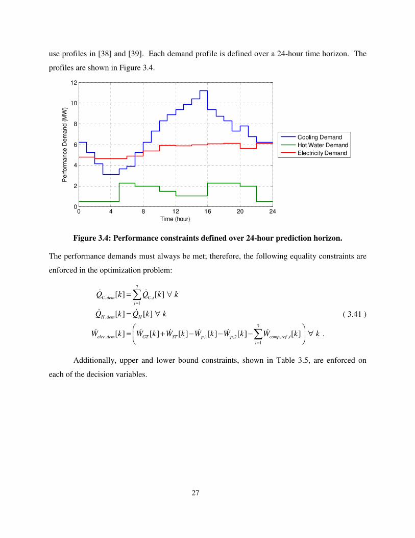
27

use profiles in [38] and [39]. Each demand profile is defined over a 24-hour time horizon. The

profiles are shown in Figure 3.4.

Figure 3.4: Performance constraints defined over 24-hour prediction horizon.

The performance demands must always be met; therefore, the following equality constraints are

enforced in the optimization problem:

, ,

, ,1 ,2 ,

7

1

1

,

,

7

[ ] [ ]

[ ] [ ]

[ ] [ ] [ ] [ ] [ ] ] .[

C dem C i

H

elec dem ST p p comp ref

i

H dem

GT i

i

k k

k k

k W

Q Q k

Q Q k

W W W Wk k k k k W k

=

=

= ∀

=

+ − −

∀

= ∀

−

∑

∑

ɺ ɺ

ɺ ɺ

ɺ ɺɺ ɺ ɺ ɺ

( 3.41 )

Additionally, upper and lower bound constraints, shown in Table 3.5, are enforced on

each of the decision variables.

0 4 8 12 16 20 240

2

4

6

8

10

12

Time (hour)

Perf

orm

an

ce

De

ma

nd (

MW

)

Cooling Demand

Hot Water Demand

Electricity Demand

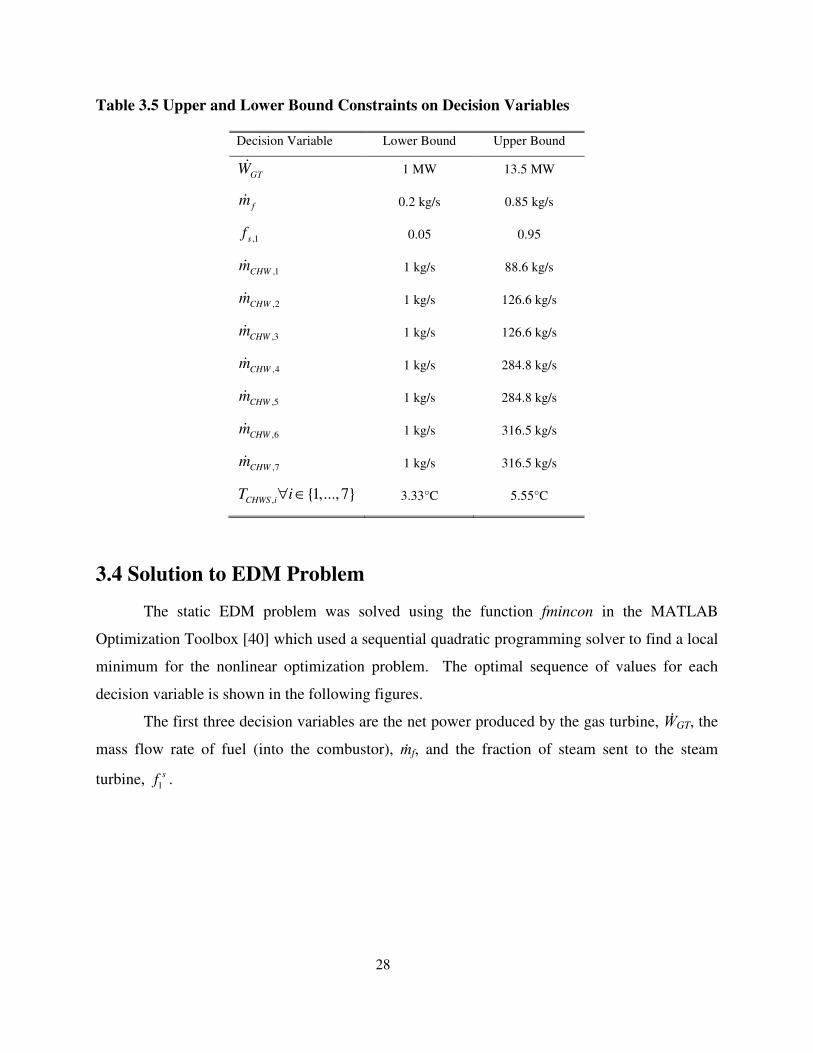
28

Table 3.5 Upper and Lower Bound Constraints on Decision Variables

Decision Variable Lower Bound Upper Bound

GTWɺ

1 MW 13.5 MW

fmɺ

0.2 kg/s 0.85 kg/s

,1sf

0.05 0.95

,1CHWmɺ 1 kg/s 88.6 kg/s







, {1,..., 7}CHWS i

T i∀ ∈

3.33°C 5.55°C

3.4 Solution to EDM Problem

The static EDM problem was solved using the function fmincon in the MATLAB

Optimization Toolbox [40] which used a sequential quadratic programming solver to find a local

minimum for the nonlinear optimization problem. The optimal sequence of values for each

decision variable is shown in the following figures.

The first three decision variables are the net power produced by the gas turbine, ẆGT, the

mass flow rate of fuel (into the combustor), ṁf, and the fraction of steam sent to the steam

turbine, 1

sf .

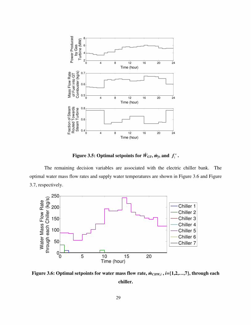
29

Figure 3.5: Optimal setpoints for ẆGT, ṁf, and 1

sf .

The remaining decision variables are associated with the electric chiller bank. The

optimal water mass flow rates and supply water temperatures are shown in Figure 3.6 and Figure

3.7, respectively.

Figure 3.6: Optimal setpoints for water mass flow rate, ṁCHW,i , i={1,2,…,7}, through each

chiller.

0 4 8 12 16 20 242

4

6

8

Time (hour)P

ow

er

Pro

du

ce

db

y G

as

Tu

rbin

e (

MW

)

0 4 8 12 16 20 240.5

0.6

0.7

Time (hour)

Ma

ss F

low

Ra

te

of F

ue

l in

to G

T

Co

mb

uste

r (k

g/s

)

0 4 8 12 16 20 240.4

0.6

0.8

Time (hour)

Fra

ctio

n o

f S

tea

m

Ro

ute

d T

ow

ard

s

Ste

am

Tu

rbin

e

0 5 10 15 200

50

100

150

200

250

Time (hour)

Wate

r M

ass F

low

Rate

thro

ug

h e

ach

Chill

er

(kg

/s)

Chiller 1

Chiller 2

Chiller 3

Chiller 4

Chiller 5

Chiller 6

Chiller 7

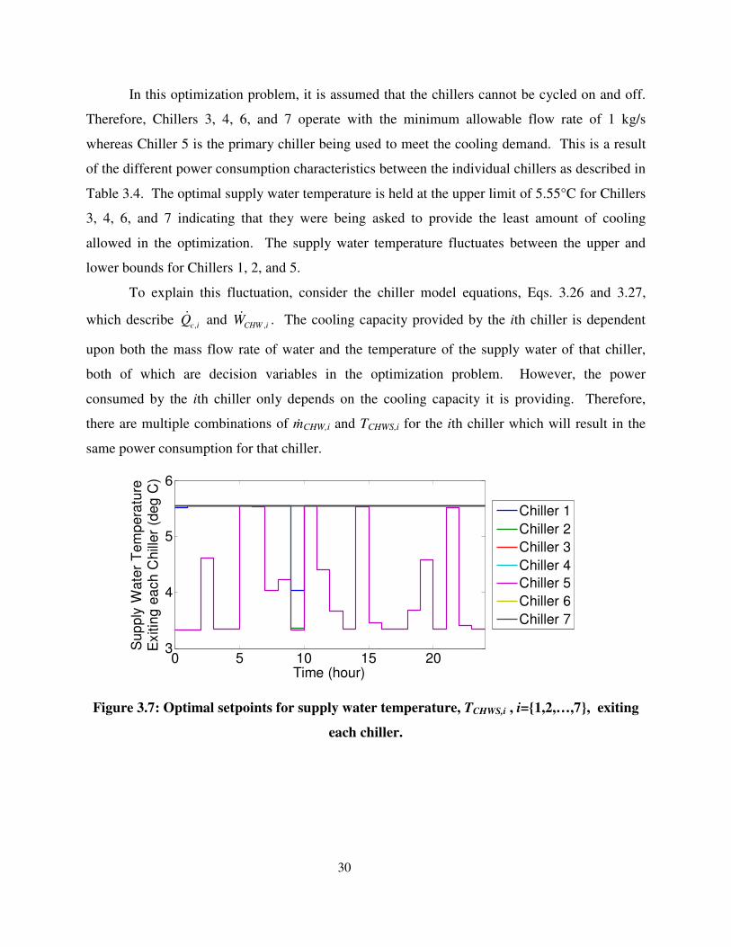
30

In this optimization problem, it is assumed that the chillers cannot be cycled on and off.

Therefore, Chillers 3, 4, 6, and 7 operate with the minimum allowable flow rate of 1 kg/s

whereas Chiller 5 is the primary chiller being used to meet the cooling demand. This is a result

of the different power consumption characteristics between the individual chillers as described in

Table 3.4. The optimal supply water temperature is held at the upper limit of 5.55°C for Chillers

3, 4, 6, and 7 indicating that they were being asked to provide the least amount of cooling

allowed in the optimization. The supply water temperature fluctuates between the upper and

lower bounds for Chillers 1, 2, and 5.

To explain this fluctuation, consider the chiller model equations, Eqs. 3.26 and 3.27,

which describe ,c iQɺ and ,CHW i

Wɺ . The cooling capacity provided by the ith chiller is dependent

upon both the mass flow rate of water and the temperature of the supply water of that chiller,

both of which are decision variables in the optimization problem. However, the power

consumed by the ith chiller only depends on the cooling capacity it is providing. Therefore,

there are multiple combinations of ṁCHW,i and TCHWS,i for the ith chiller which will result in the

same power consumption for that chiller.

Figure 3.7: Optimal setpoints for supply water temperature, TCHWS,i , i={1,2,…,7}, exiting

each chiller.

0 5 10 15 203

4

5

6

Time (hour)

Sup

ply

Wate

r T

em

pera

ture

Exitin

g e

ach C

hill

er

(deg

C)

Chiller 1

Chiller 2

Chiller 3

Chiller 4

Chiller 5

Chiller 6

Chiller 7

31

3.5 Reversible Power

3.5.1 Reversible Power for Overall CCHP System

As discussed in Chapter 2, power minimization and exergy destruction rate minimization

are related by the Gouy-Stodola theorem. Here we apply Eq. 2.8 to the entire CCHP system so

that we can derive an expression for rev

Wɺ :

( )ch

, ,

,1

0

,0

,

1

2 , ,

7

1

1

comp f f g exhaust g exhaust

p p ST co

turb H

HWR

C i

i C

mp ref i v

HWR

re

m m

W W

TW W Q

T

TQ

TW W W W

ψ ψ

=

+ − + − −

+ + − + − + =

−

−∑

ɺ ɺ

ɺ ɺ ɺ ɺ ɺ ɺ

ɺɺ ɺ

ɺ

( 3.42 )

where

4CHLHV

fW m=ɺ ɺ . ( 3.43 )

By virtue of the performance constraints imposed in the optimization problem, nearly all of the

terms in rev

Wɺ are constant (with respect to the decision variables in the optimization problem):

( )

,1 ,2 , ,

constrained to be equal to the total campus electricity demand

cspecified

in optimizationpr

7

1

0

oblem

1

rev comp ST p p comp refturb

i

H

HW

i

R

W W

TQ

T

W W W W W=

= − + − − −

− − −

∑ɺ ɺ

��

ɺ

��

ɺ

��

ɺ

�

ɺ ɺ ɺ

�constrained to be onstrained to be equal to the total equal to the total specified campus cooling campus hot water in optimization

demanddemand problem

,

,

,

70

1

1C i

i CH

g exhaus

WR

t g exm

TQ

T

ψ

=

− −

+

∑ ɺ��

ɺ

��

( )4

ch

CHLHV .haust f f

m ψ+ −ɺ

( 3.44 )

However, in this case, there are two terms which are not: , ,g exhaust g exhaustm ψɺ is the amount of flow

exergy that exits the HRSG, and ( )4

ch

CHLHVf f

m ψ−ɺ is the difference between the flow exergy

entering the combustor, ch

f fm ψɺ , and the amount of energy released during the combustion

reaction, 4CHLHV

fmɺ . It is possible for the three performance constraints to be met for different

values of , ,g exhaust g exhaustm ψɺ and ( )

4

ch

CHLHVf f

m ψ−ɺ , suggesting that minimizing exergy

32

destruction has the potential to provide a different solution than minimizing power consumption

(in terms of mass flow rate of fuel) for the overall system. A comparison between EDM and

energy consumption minimization for the CCHP system is presented in Section 3.7.

3.5.2 Reversible Power for Electric Chiller Bank

Although the reversible power for the overall CCHP system is not constant with respect

to the optimization problem, we can re-examine the reversible power for individual subsystems.

In particular, we will show that the reversible power is constant for the electric chiller bank and

introduce the concept of interchangeability wherein the exergy destruction rate and power

consumption can be combined within the same objective function to be minimized and yield the

same solution as EDM.

The exergy destruction rate for the electric chiller bank was given in Eq. 3.38 and is

restated here:

7

0

1

, ,,, 1 Cdest CHW comp ref

CHWR

ii

i

X WT

QT=

− +

=

∑ɺ ɺ ɺ . ( 3.45 )

The actual power consumed by the electric chiller bank is described by

( )7

1

, ,CHW comp ref i

i

W W=

=∑ɺ ɺ . ( 3.46 )

Applying Eq. 2.8 to the electric chiller bank yields

,

70

,

1

1 C i

i CW

rev CHW

RTW

TQ

=

−

= −∑ ɺɺ . ( 3.47 )

Therefore the EDM objective function for the CCHP system can be redefined as

,

24

, , , ,

1

[ ] [ ] [ ] [ ] [ ]

dest CHW

dest GT dest HRSG dest SL CHW rev CHWD I T

Xk

E M NWJ X k X k X k k kW−

=

= + + + −

∑ɺ

ɺ ɺ ɺ��

ɺ�

ɺ� �

( 3.48 )

where ,dest CHWXɺ has been replaced by ,CHW rev CHW

W W−ɺ ɺ . However,

24

, , ,

1

[ ] [ ] [ ] [ ]dest GT dest HREDM INT SG dest SL CHW

k

J X k X k X k kW C=

−

= + + + − ∑ ɺ ɺɺ ɺ ( 3.49 )

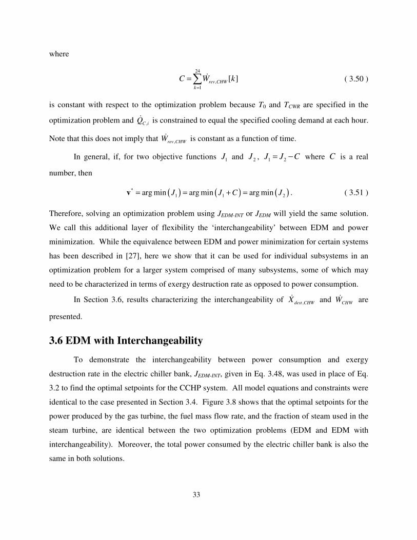
33

where

,

24

1

[ ]rev CHW

k

C kW=

=∑ ɺ ( 3.50 )

is constant with respect to the optimization problem because T0 and TCWR are specified in the

optimization problem and ,C iQɺ is constrained to equal the specified cooling demand at each hour.

Note that this does not imply that ,rev CHWWɺ is constant as a function of time.

In general, if, for two objective functions 1J and 2J , 1 2J J C= − where C is a real

number, then

( ) ( ) ( )1

*

21arg min arg min arg minCJ J J= = =+v . ( 3.51 )

Therefore, solving an optimization problem using JEDM-INT or JEDM will yield the same solution.

We call this additional layer of flexibility the ‘interchangeability’ between EDM and power

minimization. While the equivalence between EDM and power minimization for certain systems

has been described in [27], here we show that it can be used for individual subsystems in an

optimization problem for a larger system comprised of many subsystems, some of which may

need to be characterized in terms of exergy destruction rate as opposed to power consumption.

In Section 3.6, results characterizing the interchangeability of ,dest CHWXɺ and

CHWWɺ are

presented.

3.6 EDM with Interchangeability

To demonstrate the interchangeability between power consumption and exergy

destruction rate in the electric chiller bank, JEDM-INT, given in Eq. 3.48, was used in place of Eq.

3.2 to find the optimal setpoints for the CCHP system. All model equations and constraints were

identical to the case presented in Section 3.4. Figure 3.8 shows that the optimal setpoints for the

power produced by the gas turbine, the fuel mass flow rate, and the fraction of steam used in the

steam turbine, are identical between the two optimization problems (EDM and EDM with

interchangeability). Moreover, the total power consumed by the electric chiller bank is also the

same in both solutions.

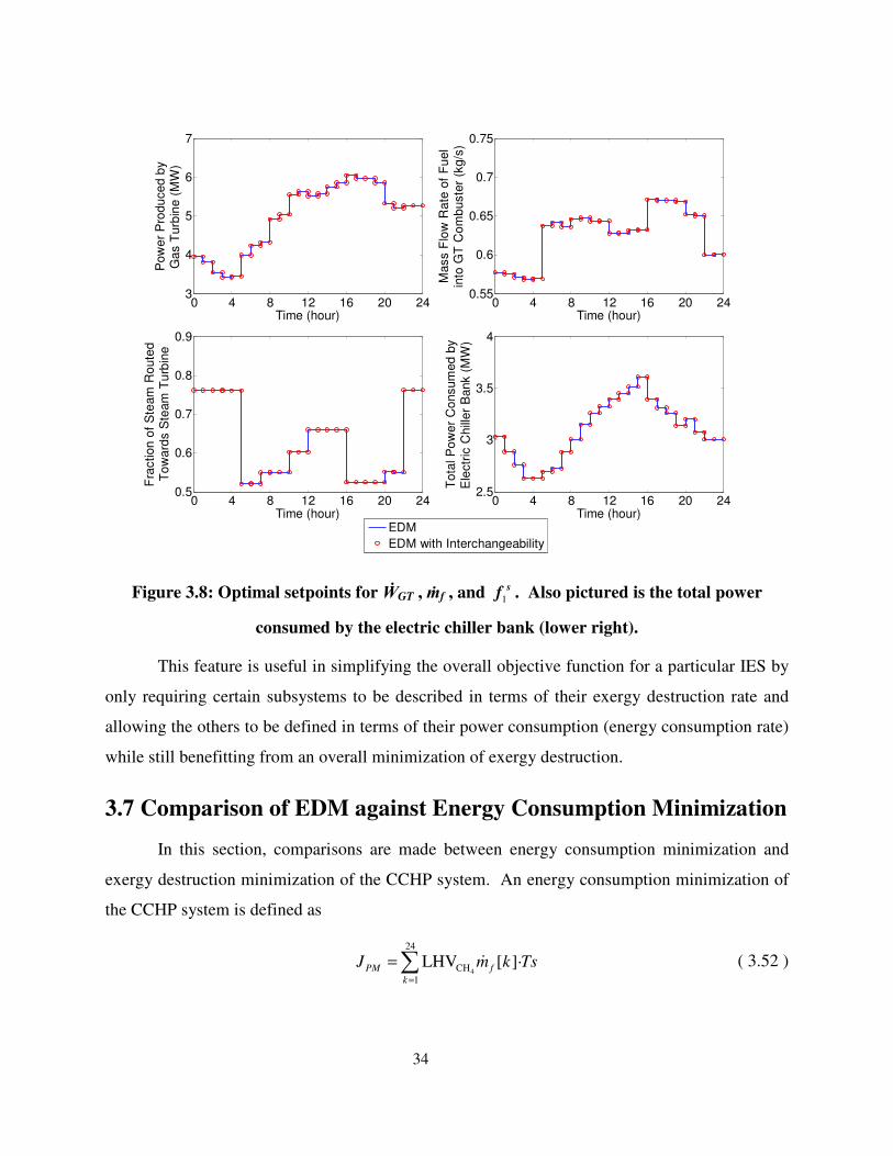
34


sf . Also pictured is the total power

consumed by the electric chiller bank (lower right).

This feature is useful in simplifying the overall objective function for a particular IES by

only requiring certain subsystems to be described in terms of their exergy destruction rate and

allowing the others to be defined in terms of their power consumption (energy consumption rate)

while still benefitting from an overall minimization of exergy destruction.

3.7 Comparison of EDM against Energy Consumption Minimization

In this section, comparisons are made between energy consumption minimization and

exergy destruction minimization of the CCHP system. An energy consumption minimization of

the CCHP system is defined as

4H

24

1

CLHV [ ·]fPM

k

m TsJ k=

=∑ ɺ ( 3.52 )

0 4 8 12 16 20 243

4

5

6

7

Time (hour)

Pow

er

Pro

du

ce

d b

yG

as T

urb

ine (

MW

)

0 4 8 12 16 20 240.55

0.6

0.65

0.7

0.75

Time (hour)

Mass F

low

Ra

te o

f F

uel

into

GT

Co

mb

uste

r (k

g/s

)

0 4 8 12 16 20 240.5

0.6

0.7

0.8

0.9

Time (hour)

Fra

ction o

f S

team

Ro

ute

dT

ow

ard

s S

team

Tu

rbin

e

0 4 8 12 16 20 242.5

3

3.5

4

Time (hour)

To

tal P

ow

er

Co

nsum

ed

by

Ele

ctr

ic C

hill

er

Bank (

MW

)

EDM

EDM with Interchangeability

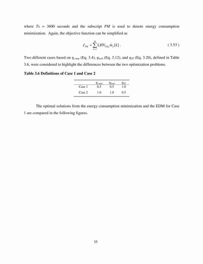
35

where Ts = 3600 seconds and the subscript PM is used to denote energy consumption

minimization. Again, the objective function can be simplified as

4H

24

1

CLHV [ ] .fPM

k

mJ k=

=∑ ɺ ( 3.53 )

Two different cases based on ηcomp (Eq. 3.4), ηturb (Eq. 3.12), and ηST (Eq. 3.20), defined in Table

3.6, were considered to highlight the differences between the two optimization problems.

Table 3.6 Definitions of Case 1 and Case 2

ηcomp ηturb ηST

Case 1 0.5 0.5 1.0

Case 2 1.0 1.0 0.5

The optimal solutions from the energy consumption minimization and the EDM for Case

1 are compared in the following figures.

36


sf as produced by EDM and energy

consumption minimization in Case 1. Also pictured is the total power consumed by the

electric chiller bank (lower right) computed using the optimal solution of each optimization

problem. Circle markers indicate that the two curves lie directly on top of one another

Figure 3.10: Optimal setpoints for ṁCHW,i and TCHWS,i , i={1,2,…,7}, using EDM in Case 1.

0 4 8 12 16 20 240

2

4

6

Time (hour)

Po

we

r P

rodu

ced b

yG

as T

urb

ine (

MW

)

0 4 8 12 16 20 240.5

0.55

0.6

0.65

0.7

Time (hour)

Ma

ss F

low

Ra

te o

f F

uel

into

GT

Com

buste

r (k

g/s

)

0 4 8 12 16 20 240.2

0.4

0.6

0.8

1

Time (hour)

Fra

ction

of

Ste

am

Ro

ute

dT

ow

ard

s S

team

Tu

rbin

e

EDM

Energy Consumption Minimization

0 4 8 12 16 20 242.5

3

3.5

4

Time (hour)

Tota

l P

ow

er

Co

nsum

ed

by

Ele

ctr

ic C

hill

er

Bank (

MW

)

0 4 8 12 16 20 240

50

100

150

200

250

Time (hour)

Wa

ter

Mass F

low

Rate

thro

ugh e

ach

Chill

er

(kg/s

)

0 4 8 12 16 20 243

3.5

4

4.5

5

5.5

6

Time (hour)

Supp

ly W

ate

r T

em

pera

ture

Exitin

g e

ach C

hill

er

(deg

C)

Chiller 1

Chiller 2

Chiller 3

Chiller 4

Chiller 5

Chiller 6

Chiller 7

37

Figure 3.11: Optimal setpoints for ṁCHW,i and TCHWS,i , i={1,2,…,7}, using energy

consumption minimization in Case 1.

Both objective functions, JEDM and JPM, were evaluated using the optimal solution from both the

EDM and the energy consumption minimization. These results are shown in Table 3.7 where the

percent difference is defined as

( ) ( )

( )

* *

*% 100 .

EDM PM

EDM

J differ

J

Jence

−×=

v v

v ( 3.54 )

Table 3.7 JEDM and JPM Evaluated Using Optimal Solutions from both EDM and PM in

Case 1

Objective

Function

Exergy Destruction

Minimization (kW)

Energy Consumption

Minimization (kW)

Percent

Difference (%)

JEDM 537,800 549420 -2.16

JPM 739,940 725380 1.97

As expected, in Case 1, the EDM outperformed the energy consumption minimization

with respect to exergy destruction whereas the energy consumption minimization outperformed

the EDM with respect to energy consumption. Figure 3.9 shows that the EDM significantly

favored producing power with the steam turbine over the gas turbine by choosing to operate the

gas turbine at its lower bound of 1MW for a large portion of the 24-hour time horizon. This is

consistent with the fact that the steam turbine was designed to be significantly more efficient

than the gas turbine in Case 1. The effects of the difference between ηcomp, ηturb, and ηST manifest

themselves explicitly in JEDM via the terms Ẋdest,GT and Ẋdest,SL. As mentioned in Chapter 2, these

0 4 8 12 16 20 240

50

100

150

200

250

Time (hour)

Wate

r M

ass F

low

Rate

thro

ug

h e

ach C

hill

er

(kg

/s)

0 4 8 12 16 20 243

3.5

4

4.5

5

5.5

6

Time (hour)

Su

pply

Wa

ter

Tem

pe

ratu

reE

xitin

g e

ach

Chill

er

(de

g C

)

Chiller 1

Chiller 2

Chiller 3

Chiller 4

Chiller 5

Chiller 6

Chiller 7

38

two terms are naturally weighted against one another because they describe the same physical

quantity, rate of exergy destruction, for two interacting systems. In JPM the effects of the

difference between ηcomp, ηturb, and ηST only manifest themselves through the equality constraints

to meet the specified cooling, heating, and electricity demands.

Next we compare energy consumption minimization and EDM when the gas turbine is

significantly more efficient than the steam turbine (described as Case 2 in Table 3.6).


sf as produced by EDM and energy

consumption minimization in Case 2. Also pictured is the total power consumed by the

electric chiller bank (lower right) computed using the optimal solution of each optimization

problem. Circle markers indicate that the two curves lie directly on top of one another.

0 4 8 12 16 20 244

6

8

10

Time (hour)

Pow

er

Pro

du

ce

d b

yG

as T

urb

ine (

MW

)

EDM

Energy Consumption Minimization

0 4 8 12 16 20 240.5

0.55

0.6

0.65

0.7

Time (hour)

Mass F

low

Ra

te o

f F

uel

into

GT

Co

mb

uste

r (k

g/s

)

0 4 8 12 16 20 240

0.2

0.4

0.6

0.8

Time (hour)

Fra

ctio

n o

f S

tea

m R

ou

ted

Tow

ard

s S

tea

m T

urb

ine

0 4 8 12 16 20 242.5

3

3.5

4

Time (hour)

Tota

l P

ow

er

Con

su

me

d b

yE

lectr

ic C

hill

er

Ba

nk (

MW

)

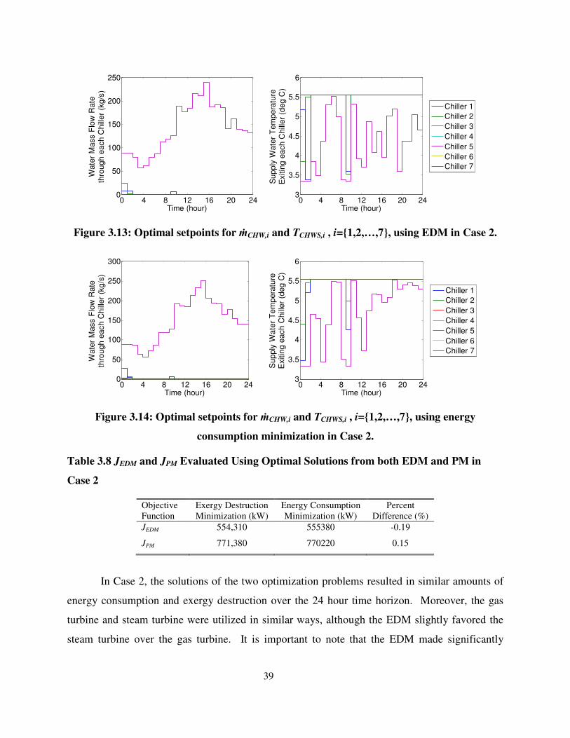
39

Figure 3.13: Optimal setpoints for ṁCHW,i and TCHWS,i , i={1,2,…,7}, using EDM in Case 2.

Figure 3.14: Optimal setpoints for ṁCHW,i and TCHWS,i , i={1,2,…,7}, using energy

consumption minimization in Case 2.

Table 3.8 JEDM and JPM Evaluated Using Optimal Solutions from both EDM and PM in

Case 2

Objective

Function

Exergy Destruction

Minimization (kW)

Energy Consumption

Minimization (kW)

Percent

Difference (%)

JEDM 554,310 555380 -0.19

JPM 771,380 770220 0.15

In Case 2, the solutions of the two optimization problems resulted in similar amounts of

energy consumption and exergy destruction over the 24 hour time horizon. Moreover, the gas

turbine and steam turbine were utilized in similar ways, although the EDM slightly favored the

steam turbine over the gas turbine. It is important to note that the EDM made significantly

0 4 8 12 16 20 240

50

100

150

200

250

Time (hour)

Wate

r M

ass F

low

Rate

thro

ug

h e

ach C

hill

er

(kg

/s)

0 4 8 12 16 20 243

3.5

4

4.5

5

5.5

6

Time (hour)

Su

pply

Wa

ter

Tem

pe

ratu

reE

xitin

g e

ach

Chill

er

(de

g C

)

Chiller 1

Chiller 2

Chiller 3

Chiller 4

Chiller 5

Chiller 6

Chiller 7

0 4 8 12 16 20 240

50

100

150

200

250

300

Time (hour)

Wa

ter

Ma

ss F

low

Ra

teth

rou

gh

ea

ch

Ch

ille

r (k

g/s

)

0 4 8 12 16 20 243

3.5

4

4.5

5

5.5

6

Time (hour)

Su

pply

Wa

ter

Te

mp

era

ture

Exitin

g e

ach

Chill

er

(de

g C

)

Chiller 1

Chiller 2

Chiller 3

Chiller 4

Chiller 5

Chiller 6

Chiller 7

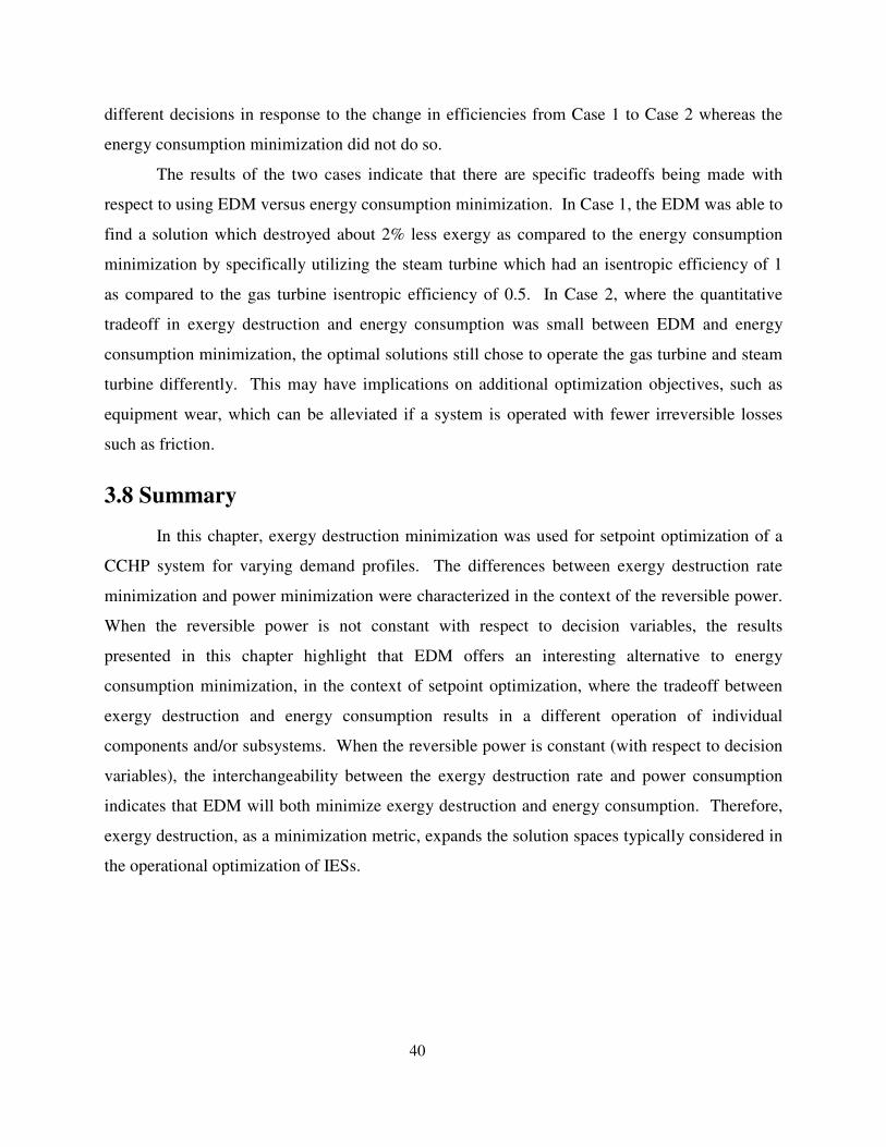
40

different decisions in response to the change in efficiencies from Case 1 to Case 2 whereas the

energy consumption minimization did not do so.

The results of the two cases indicate that there are specific tradeoffs being made with

respect to using EDM versus energy consumption minimization. In Case 1, the EDM was able to

find a solution which destroyed about 2% less exergy as compared to the energy consumption

minimization by specifically utilizing the steam turbine which had an isentropic efficiency of 1

as compared to the gas turbine isentropic efficiency of 0.5. In Case 2, where the quantitative

tradeoff in exergy destruction and energy consumption was small between EDM and energy

consumption minimization, the optimal solutions still chose to operate the gas turbine and steam

turbine differently. This may have implications on additional optimization objectives, such as

equipment wear, which can be alleviated if a system is operated with fewer irreversible losses

such as friction.

3.8 Summary

In this chapter, exergy destruction minimization was used for setpoint optimization of a

CCHP system for varying demand profiles. The differences between exergy destruction rate

minimization and power minimization were characterized in the context of the reversible power.

When the reversible power is not constant with respect to decision variables, the results

presented in this chapter highlight that EDM offers an interesting alternative to energy

consumption minimization, in the context of setpoint optimization, where the tradeoff between

exergy destruction and energy consumption results in a different operation of individual

components and/or subsystems. When the reversible power is constant (with respect to decision

variables), the interchangeability between the exergy destruction rate and power consumption

indicates that EDM will both minimize exergy destruction and energy consumption. Therefore,

exergy destruction, as a minimization metric, expands the solution spaces typically considered in

the operational optimization of IESs.

41

Chapter 4

EDM-Based Setpoint Optimization and Control of a

VCC System

In this chapter, the exergy destruction minimization (EDM) framework outlined in

Chapter 2 is applied to a vapor-compression cycle (VCC) system. After a brief introduction to

VCC systems, a static setpoint optimization problem is formulated. In order to operate an

experimental VCC system at the optimized setpoints, a feedforward plus feedback control

approach is described and then implemented experimentally. The experimental results are also

compared to design point operation of the same system to quantify how optimization and control

of the VCC system can lead to improvements in efficiency.

4.1 Introduction to Vapor-Compression Cycle Systems

VCC systems are used to remove heat from a low-temperature (TL) environment and

reject it to a high-temperature (TH) reservoir (typically ambient air). A standard VCC system

contains four components – a compressor, a condenser, an expansion device, and an evaporator –

and operates between high and low temperature reservoirs as shown in Figure 4.1.

The basic operation of a VCC system is as follows. Beginning at transition point 1, near-

saturated refrigerant vapor is compressed to a higher temperature and pressure. The superheated

refrigerant vapor enters the condenser at transition point 2 where it loses energy to ambient air

(or another secondary fluid) passing over the condenser coil. The refrigerant leaves as a

subcooled liquid and then enters an expansion device at transition point 3 (e.g. thermostatic

expansion valve, electronic expansion valve, capillary tube, etc.) where it undergoes a rapid drop

in pressure and temperature. At transition point 4, the refrigerant enters the evaporator as a two-

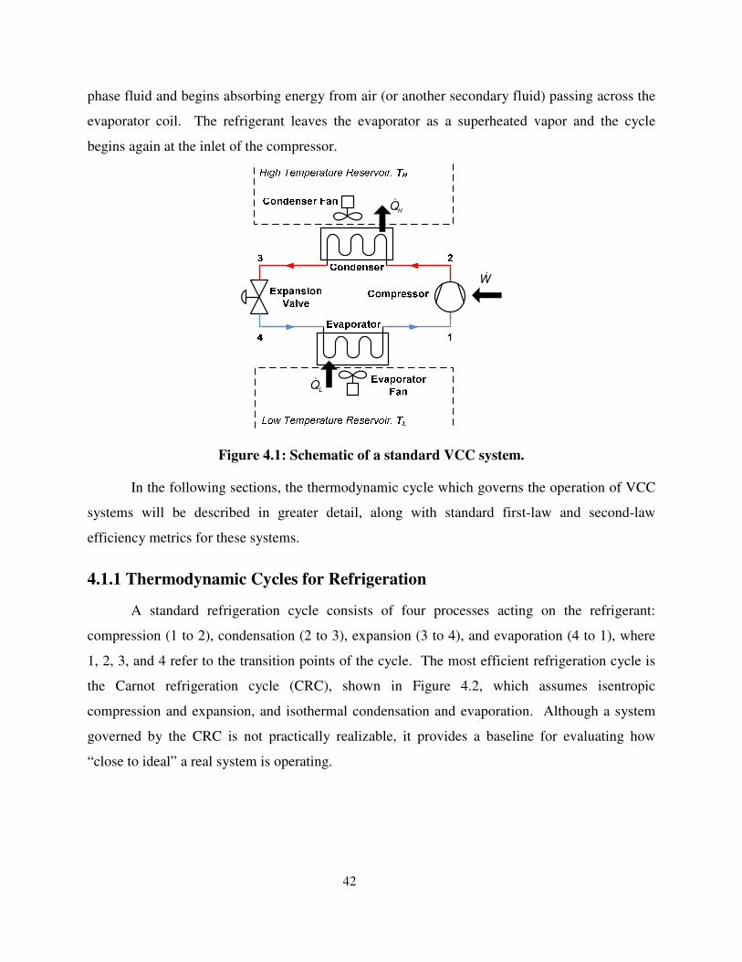
42

phase fluid and begins absorbing energy from air (or another secondary fluid) passing across the

evaporator coil. The refrigerant leaves the evaporator as a superheated vapor and the cycle

begins again at the inlet of the compressor.

Figure 4.1: Schematic of a standard VCC system.

In the following sections, the thermodynamic cycle which governs the operation of VCC

systems will be described in greater detail, along with standard first-law and second-law

efficiency metrics for these systems.

4.1.1 Thermodynamic Cycles for Refrigeration

A standard refrigeration cycle consists of four processes acting on the refrigerant:

compression (1 to 2), condensation (2 to 3), expansion (3 to 4), and evaporation (4 to 1), where

1, 2, 3, and 4 refer to the transition points of the cycle. The most efficient refrigeration cycle is

the Carnot refrigeration cycle (CRC), shown in Figure 4.2, which assumes isentropic

compression and expansion, and isothermal condensation and evaporation. Although a system

governed by the CRC is not practically realizable, it provides a baseline for evaluating how

“close to ideal” a real system is operating.

ɺW

ɺL

Q

ɺH

Q

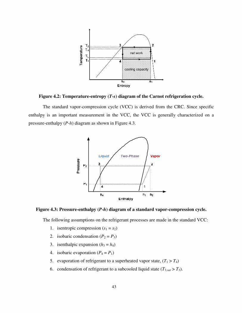
43

Figure 4.2: Temperature-entropy (T-s) diagram of the Carnot refrigeration cycle.

The standard vapor-compression cycle (VCC) is derived from the CRC. Since specific

enthalpy is an important measurement in the VCC, the VCC is generally characterized on a

pressure-enthalpy (P-h) diagram as shown in Figure 4.3.

Figure 4.3: Pressure-enthalpy (P-h) diagram of a standard vapor-compression cycle.

The following assumptions on the refrigerant processes are made in the standard VCC:

1. isentropic compression (s1 = s2)

2. isobaric condensation (P2 = P3)

3. isenthalpic expansion (h3 = h4)

4. isobaric evaporation (P4 = P1)

5. evaporation of refrigerant to a superheated vapor state, (T1 > T4)

6. condensation of refrigerant to a subcooled liquid state (T3,sat > T3).

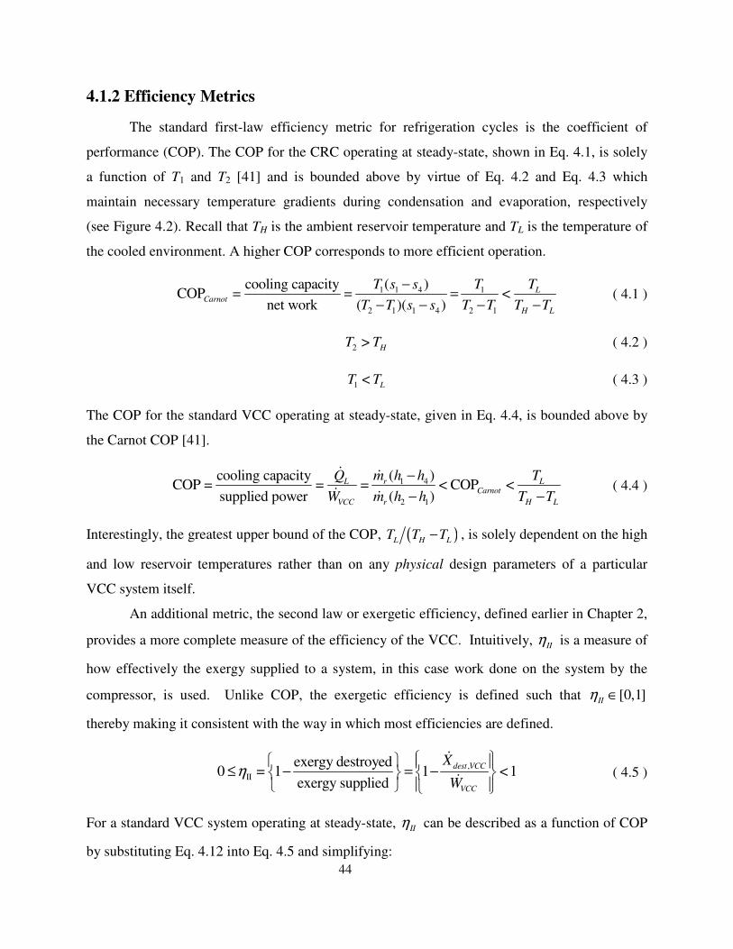
44

4.1.2 Efficiency Metrics

The standard first-law efficiency metric for refrigeration cycles is the coefficient of

performance (COP). The COP for the CRC operating at steady-state, shown in Eq. 4.1, is solely

a function of T1 and T2 [41] and is bounded above by virtue of Eq. 4.2 and Eq. 4.3 which

maintain necessary temperature gradients during condensation and evaporation, respectively

(see Figure 4.2). Recall that TH is the ambient reservoir temperature and TL is the temperature of

the cooled environment. A higher COP corresponds to more efficient operation.

1 1 4 1

2 1 1 4 2 1

( )cooling capacityCOP = = <

net work ( )( )

LCarnot

H L

T s s T T

T T s s T T T T

−=

− − − − ( 4.1 )

2 > HT T ( 4.2 )

1 < LT T ( 4.3 )

The COP for the standard VCC operating at steady-state, given in Eq. 4.4, is bounded above by

the Carnot COP [41].

1 4

2 1

( )cooling capacityCOP = = = < COP <

supplied power ( )VC

L r LCarnot

r H LC

Q m h h T

W m h h T T

−

− −

ɺ ɺɺ ɺ

( 4.4 )

Interestingly, the greatest upper bound of the COP, ( )L H LT T T− , is solely dependent on the high

and low reservoir temperatures rather than on any physical design parameters of a particular

VCC system itself.

An additional metric, the second law or exergetic efficiency, defined earlier in Chapter 2,

provides a more complete measure of the efficiency of the VCC. Intuitively, IIη is a measure of

how effectively the exergy supplied to a system, in this case work done on the system by the

compressor, is used. Unlike COP, the exergetic efficiency is defined such that [0,1]IIη ∈

thereby making it consistent with the way in which most efficiencies are defined.

,

II

exergy destroyed0 = 1 1 <1

exergy supplied

dest VCC

VCC

X

Wη

≤ − = −

ɺ

ɺ ( 4.5 )

For a standard VCC system operating at steady-state, IIη can be described as a function of COP

by substituting Eq. 4.12 into Eq. 4.5 and simplifying:

45

II

COP0 = <1.

L

H L

T

T T

η≤

−

( 4.6 )

4.1.3 Control of VCC Systems

Electronic actuators, such as variable-speed compressors, electronic expansion valves

(EEVs), and variable-speed fans, have long been advocated as integral to improving the

efficiency of VCC systems [42] [43] [44]. Moreover, these actuators provide the control engineer

with access to the various degrees of freedom (DOFs) of the system and consequently, the ability

to operate the system without cycling the compressor. Therefore, there is significant potential for

improving the partial-load operational efficiency of any given VCC system through optimization

and control of these available DOFs.

Conducting a setpoint optimization relies on an understanding of the DOFs which are

available to be optimized. As will be discussed in Section 4.2.1, the standard VCC has five

optimization DOFs. However, research in setpoint optimization of VCC system operation has

been characterized by the number of DOFs being constrained a priori [45] [46] [47]. In this

chapter, we are specifically interested in considering all available DOFs of the VCC system.

Finally, beyond the optimization of operation setpoints, a control framework is necessary

to ensure that the system does indeed operate optimally. The typical choice of feedback control

variables for VCC systems are evaporator refrigerant pressure or saturation temperature, and

evaporator superheat, controlled by the compressor and EEV, respectively [44] [48] [49] [50].

However, this particular choice of input-output control variables is rooted in the legacy of

mechanical control of VCC systems. Before the advent of electronic control, mechanical control

devices, such as the thermostatic expansion valve (TEV), were developed in which the sensor

and actuator were mechanically coupled and only tunable manually offline. Today, with

electronic sensing and actuation, the sensor and actuator are decoupled. In [51], the authors

explored this flexibility and, using a different choice of input-output pairings for a standard VCC

system, designed and implemented a decentralized controller which accurately tracked given

reference commands. The control framework presented in this chapter is independent of a

particular choice of input-output pairings, instead introducing a design variable Λ which allows

46

the user to specify his/her choice of input-output pairings for a particular system hardware

configuration.

4.2 Optimization Problem Formulation

4.2.1 Determining the Decision Variables

Based on the constitutive relationships between pressure, temperature, entropy, etc., [16]

the VCC has 8 thermodynamic degrees of freedom (DOFs) – two DOFs for each of the four

transition points in the cycle. However, the four equality constraints (specified in the previous

section) which arise from isentropic, isobaric, and isenthalpic assumptions constrain 4 of these

DOFs. Therefore, the three specific enthalpies of the cycle, {h1, h2, h3=h4}, and any one of the

following three quantities, {P1, P2, T1}, uniquely define the remaining thermodynamic states at

each of the transition points. Moreover, to actually compute critical quantities of interest, such

as the amount of cooling that is achieved (Eq. 4.7) or the amount of power consumed by the

compressor (Eq. 4.8), there is one additional DOF which must be considered: the refrigerant

mass flow rate, rmɺ . This DOF is a fluid dynamic variable, rather than a thermodynamic variable,

and is not captured in the P-h diagram of the VCC.

1 4= ( )L r

Q m h h−ɺ ɺ ( 4.7 )

( )2 1=CC k rV

W hW m h= −ɺɺ ɺ ( 4.8 )

4.2.2 Objective Function Development

For VCC system setpoint optimization, we will again consider two primary objectives: a

performance objective and an efficiency objective. For a VCC system, the performance

objective is to achieve some desired cooling capacity. Following the framework outlined in

Chapter 2, the optimization problem will be formulated as an exergy destruction minimization

(EDM) problem with the performance objective enforced as an equality constraint. Whereas in

Chapter 3 the objective was to minimize the total exergy destroyed over a 24-hour time period,

here we do not consider a time-varying performance objective. Therefore, the objective function

JVCC is defined as

47

,VCC dest VCCJ X= ɺ . ( 4.9 )

Since the VCC is a closed thermodynamic cycle, the exergy rate balance for a closed

system (control mass) is used to derive an expression for the total rate of exergy destruction:

ch0

01 j dest

j j

TdX dVQ W P X X

dt T dt

= − − − +

−

∑ ɺ ɺ ɺ ɺ . ( 4.10 )

During steady-state operation of the VCC system, the following simplifications can be made to

Eq. 4.10:

dX

dt

001 j

j j

T dVQ W P

T dt

= − − −

∑ ɺ ɺ ch

X

+

ɺdestX− ɺ . ( 4.11 )

Moreover, by assuming the ambient temperature, TH, is the reference temperature, T0, Eq. 4.11

reduces to

, = ( ) 1 Hdest VCC VCC L

L

TX W Q

T

− − + −

ɺɺ ɺ ( 4.12 )

where Tj has been replaced by TL. Equation 4.12 is evaluated with TH and TL in degrees Kelvin.

Substituting Eq. 4.7 and Eq. 4.8 into Eq. 4.12 yields

( ), 1 14 2= ( ) 1 0 .Hdest V rCC r

L

TmX m h h

Th h

− − + ≥ −

ɺ ɺ ɺ ( 4.13 )

As discussed in Chapter 2, the exergy destruction rate is nonnegative by definition. Therefore,

the theoretical minimum value of JVCC is zero, and its solution is defined as

( ) ( )* * * * *

4 1

*

1

5

2arg minv

v VCC

T

J h h h P m= = ∈ɺ ℝ . ( 4.14 )

subject to a number of different constraints which will be defined in the next section.

4.2.3 Defining Constraints

There are a number of different constraints which need to be defined for this optimization

problem. They include performance, thermodynamic, and design constraints, in addition to

48

upper and lower bound constraints on the individual decision variables. Each of these different

constraints will be described in the following subsections.

4.2.3.1 Performance Constraint

In this optimization problem, the performance objective of achieving a desired cooling

capacity is enforced as the following equality constraint:

1 4= ( )rdes L

C mQ h h= −ɺɺ . ( 4.15 )

Note that if some deviation away from the desired cooling capacity is allowed, the performance

constraint can be defined as an inequality constraint of the form

1 4( )des r

C m h h γ− − ≤ɺ ( 4.16 )

where γ is the maximum allowable error between the desired and achieved cooling capacities.

4.2.3.2 Thermodynamic Constraints

The following thermodynamic constraints must be enforced in the optimization of a

standard VCC system:

1. 1 2h h< 2. 4 1h h<

3. 1 LT T< 4. 3 HT T>

5. 1 4 0T T− > 6. 3, 3

0sat

TT − >

where T3,sat is the saturated refrigerant temperature at P2. The first two constraints ensure that

compression and evaporation, respectively, occur. The third and fourth constraints impose the

correct temperature gradients during evaporation and condensation, respectively. Note that in

the VCC, the refrigerant temperature at the outlet of the condenser is denoted T3 whereas in the

CRC it is T2. The fifth constraint ensures that only refrigerant vapor is compressed. Finally, the

sixth constraint ensures that only refrigerant liquid is expanded.

4.2.3.3 Design Constraints

The hardware in a particular VCC system constrains the setpoints achievable by that

system when it is operated. The design constraints imposed by the two heat exchangers

49

(evaporator and condenser) as well as their corresponding fans are defined by the following

inequalities:

1 4 ,max 4

,

( ) ( ) ( ) ,r L

L L max

L

Q

Am

Q

Uh h T T

≤

− −≤

ɺ

ɺ

ɺ ( 4.17 )

and

2 4 ,max 3

,

( ) ( ) ( ) ,

H

r H

H max

Hm

Q Q

UAh h T T

≤

− −≤

ɺ

ɺ

ɺ ( 4.18 )

where (UA)L,max and (UA)H,max are the maximum overall heat transfer coefficients across the

evaporator and condenser, respectively. These coefficients can be estimated using heat transfer

correlations and a thermal resistance circuit as shown in Figure 4.4 [52]. In order to simplify the

estimation of the maximum UA values for the evaporator and condenser, respectively, the

following assumptions are made:

1. ,a emɺ and ,a c

mɺ are assumed to be their maximum possible values based on the

design of the evaporator and condenser fans, respectively,

2. the refrigerant in each heat exchanger is entirely a two-phase fluid,

3. and are constant throughout the condenser and evaporator, respectively,

4. fin heat transfer is one-dimensional.

Figure 4.4: Thermal resistance circuit used to estimate overall heat transfer coefficients for

the evaporator and condenser.

The correlations used to estimate the heat transfer coefficients rα and aα for the specific

evaporator and condenser considered in the experimental case study are described in [53]. The

fraction of the outer tube surface area covered by fins is denoted by Fa.

HT LT

50

1 1 1

=(1 )r i o a a o

t

UA A kA F Aα α

+ +

− ( 4.19 )

4.2.3.4 Upper and Lower Bound Constraints

The final set of constraints which is enforced in the optimization problem consists of

upper and lower bound constraints on the decision variables. The thermodynamic decision

variables in the optimization of any VCC system will be bounded (above and below) by the fluid

properties of the refrigerant used in that particular VCC system [54]. For the case study

presented in this chapter, refrigerant R134a will be considered. The bound on the refrigerant

mass flow rate, ɺ rm , is based on typical performance characteristics of R134a as reported in the

ASHRAE Handbook [54] but will also depend on the physical hardware of the system being

optimized.

Table 4.1: Upper and Lower Bound Constraints on Decision Variables for R134a

Decision

Variable Units Lower Bound Upper Bound

1h kJ/kg 220 350

2h kJ/kg 220 350

4h kJ/kg 20 220

1P kPa 150 550

rmɺ kg/s 0.00 0.00611

4.3 Control Synthesis

In this section, we characterize the steady-state behavior of a standard VCC system and

create a control framework for realizing the optimized operation setpoints on an actual VCC

system.

The control inputs for a standard VCC system are the electronic expansion valve (EEV)

aperture, av, the compressor speed, ωk and the evaporator and condenser fan speeds, ωf,e and ωf,c

respectively. It is assumed that the compressor, and evaporator and condenser fans, are variable-

speed. The vector of control input variables, u, is defined as

( ) 4

, ,

T

v k f e f ca ω ω ω= ∈u ℝ . ( 4.20 )

51

The four thermodynamic optimization variables, h1, h2, h4, and P1, are rewritten via

constitutive relationships [16] in terms of an equivalent set of pressures and temperatures which

can be measured on a physical system. Therefore, the vector of decision variables is redefined as

( )1 2 1

5

3v

T

rP P T T m= ∈ɺ ℝ ( 4.21 )

where

( ) ( )* * 5* * * *

1 2 1 3arg minv

vT

V rCCJ P P T mT= = ∈ɺ ℝ . ( 4.22 )

The decision variables and the control inputs are related during steady-state operation of the

standard VCC system by the following 9 equations:

1 1 2ˆ = ( , , )

vvK f a P P , ( 4.23 )

2 1 2ˆ = ( , , )vo kl f P Pωη , ( 4.24 )

3 1 2 ,

( ) = ( , , , )r f eL

UA f P P m ωɺ , ( 4.25 )

4 2 ,

( ) = ( , , )r f cH

UA f P m ωɺ , ( 4.26 )

4 1 4

ˆ= ( ) ( ) = ( )

L L rLQ UA T T m h h− −ɺ ɺ , ( 4.27 )

3 2 4

ˆ= ( ) ( ) = ( )

H H rHQ UA T T m h h− −ɺ ɺ , ( 4.28 )

, 3 2 1

ˆ ˆ= ( )r v vm K P Pρ −ɺ , ( 4.29 )

, 1

ˆ ˆ=r k vol k km η δ ω ρɺ , ( 4.30 )

, ,

ˆ ˆ=r v r km mɺ ɺ , ( 4.31 )

where Kv is the valve flow coefficient, ηvol is the compressor volumetric efficiency, and (UA)L

and (UA)H are the overall heat transfer coefficients [52] at the low and high temperature

reservoirs, respectively. The functions fi, i={1,2,3,4} are empirically-derived nonlinear

relationships; additional details are provided in [53].

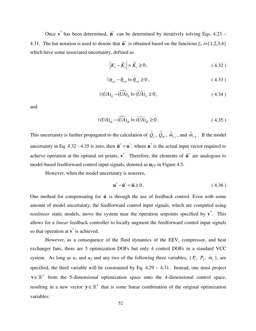
52

Once v* has been determined, *u can be determined by iteratively solving Eqs. 4.23 –

4.31. The hat notation is used to denote that *u is obtained based on the functions fi, i={1,2,3,4}

which have some associated uncertainty, defined as

ˆ 0v v vK K K− = ≥ɶ , ( 4.32 )

ˆ| |= 0vol vol volη η η− ≥ɶ , ( 4.33 )

�| ( ) ( ) |= ( ) 0L L L

UA UA UA− ≥ , ( 4.34 )

and

�| ( ) ( ) |= ( ) 0H H H

UA UA UA− ≥ . ( 4.35 )

This uncertainty is further propagated to the calculation of ˆ

LQɺ , ˆ

HQɺ , ,ˆ

r vmɺ , and ,ˆ

r kmɺ . If the model

uncertainty in Eq. 4.32 - 4.35 is zero, then * *ˆ =u u , where u* is the actual input vector required to

achieve operation at the optimal set points, v*. Therefore, the elements of *u are analogous to

model-based feedforward control input signals, denoted as uFF in Figure 4.5.

However, when the model uncertainty is nonzero,

* *ˆ 0− = ≥u u uɶ . ( 4.36 )

One method for compensating for uɶ is through the use of feedback control. Even with some

amount of model uncertainty, the feedforward control input signals, which are computed using

nonlinear static models, move the system near the operation setpoints specified by v*. This

allows for a linear feedback controller to locally augment the feedforward control input signals

so that operation at v* is achieved.

However, as a consequence of the fluid dynamics of the EEV, compressor, and heat

exchanger fans, there are 5 optimization DOFs but only 4 control DOFs in a standard VCC

system. As long as u1 and u2 and any two of the following three variables, { 1P , 2P , ɺ rm }, are

specified, the third variable will be constrained by Eq. 4.29 – 4.31. Instead, one must project

5∈v ℝ from the 5-dimensional optimization space onto the 4-dimensional control space,

resulting in a new vector 4∈y ℝ that is some linear combination of the original optimization

variables:

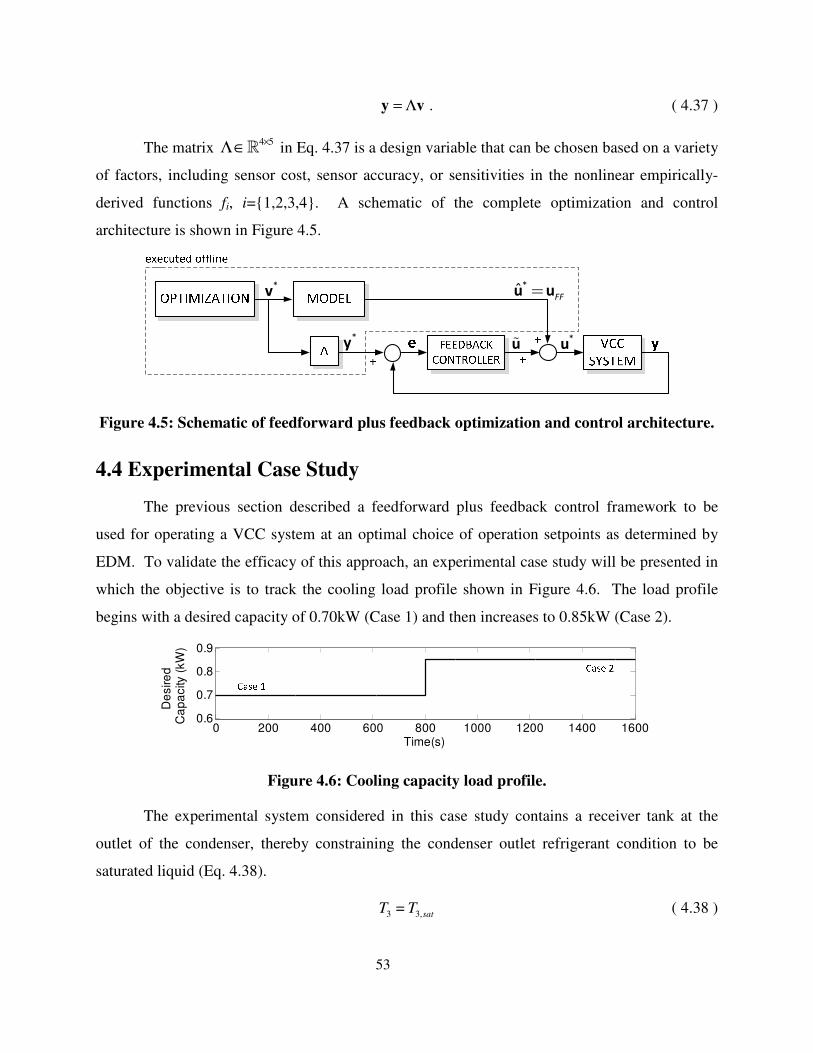
53

.= Λy v ( 4.37 )

The matrix 4 5×Λ∈ℝ in Eq. 4.37 is a design variable that can be chosen based on a variety

of factors, including sensor cost, sensor accuracy, or sensitivities in the nonlinear empirically-

derived functions fi, i={1,2,3,4}. A schematic of the complete optimization and control

architecture is shown in Figure 4.5.

Figure 4.5: Schematic of feedforward plus feedback optimization and control architecture.

4.4 Experimental Case Study

The previous section described a feedforward plus feedback control framework to be

used for operating a VCC system at an optimal choice of operation setpoints as determined by

EDM. To validate the efficacy of this approach, an experimental case study will be presented in

which the objective is to track the cooling load profile shown in Figure 4.6. The load profile

begins with a desired capacity of 0.70kW (Case 1) and then increases to 0.85kW (Case 2).

Figure 4.6: Cooling capacity load profile.

The experimental system considered in this case study contains a receiver tank at the

outlet of the condenser, thereby constraining the condenser outlet refrigerant condition to be

saturated liquid (Eq. 4.38).

3 3,=sat

T T ( 4.38 )

uɶ

v*

u*

u u*

ˆFF

=

y*

0 200 400 600 800 1000 1200 1400 16000.6

0.7

0.8

0.9

De

sire

d

Ca

pa

city

(kW

)

Time(s)

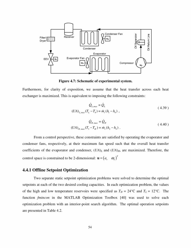
54

Figure 4.7: Schematic of experimental system.

Furthermore, for clarity of exposition, we assume that the heat transfer across each heat

exchanger is maximized. This is equivalent to imposing the following constraints:

,

, 4 1 4

=

( ) ( ) = ( ) ,

L max L

L max L r

Q Q

UA T T m h h− −

ɺ ɺ

ɺ ( 4.39 )

,

, 3 2 4

=

( ) ( ) = ( ) .

H max H

H max H r

Q Q

UA T T m h h− −

ɺ ɺ

ɺ ( 4.40 )

From a control perspective, these constraints are satisfied by operating the evaporator and

condenser fans, respectively, at their maximum fan speed such that the overall heat transfer

coefficients of the evaporator and condenser, (UA)L and (UA)H, are maximized. Therefore, the

control space is constrained to be 2-dimensional: ( )T

v ka ω=u

4.4.1 Offline Setpoint Optimization

Two separate static setpoint optimization problems were solved to determine the optimal

setpoints at each of the two desired cooling capacities. In each optimization problem, the values

of the high and low temperature reservoirs were specified as TH = 24°C and TL = 12°C. The

function fmincon in the MATLAB Optimization Toolbox [40] was used to solve each

optimization problem with an interior-point search algorithm. The optimal operation setpoints

are presented in Table 4.2.

Condenser

Evaporator

ReceiverCondenser Fan

Evaporator Fan

Compressor

u4

u3u2

Filter/

Dryer

EEV u1

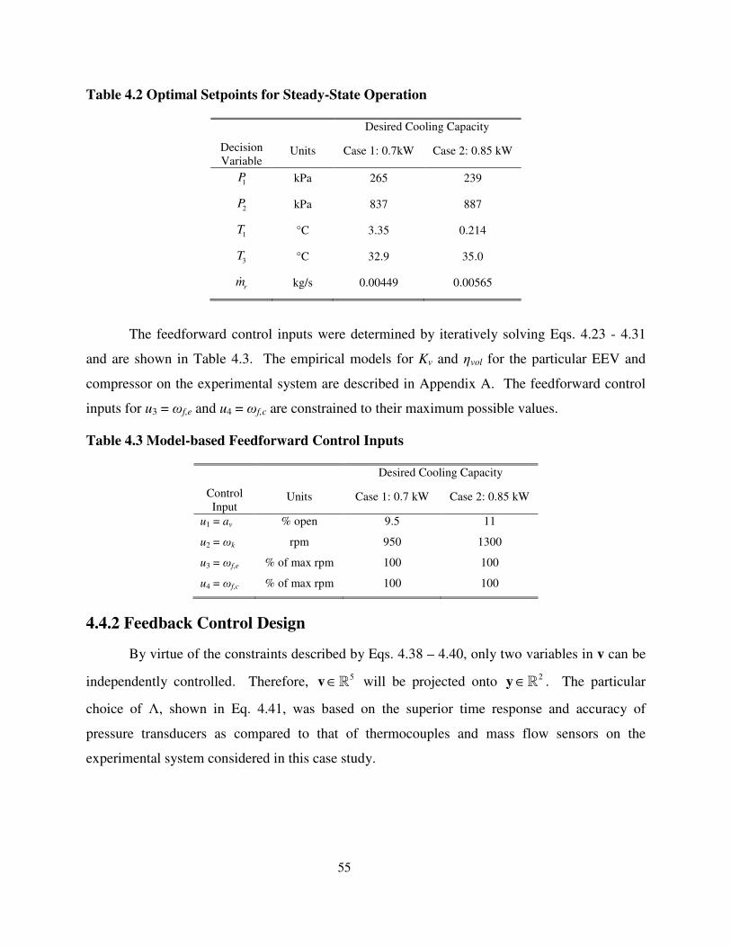
55

Table 4.2 Optimal Setpoints for Steady-State Operation

Desired Cooling Capacity

Decision

Variable Units Case 1: 0.7kW Case 2: 0.85 kW

1P kPa 265 239

2P kPa 837 887

1T °C 3.35 0.214

3T

°C 32.9 35.0

rmɺ kg/s 0.00449 0.00565

The feedforward control inputs were determined by iteratively solving Eqs. 4.23 - 4.31

and are shown in Table 4.3. The empirical models for Kv and ηvol for the particular EEV and

compressor on the experimental system are described in Appendix A. The feedforward control

inputs for u3 = ωf,e and u4 = ωf,c are constrained to their maximum possible values.

Table 4.3 Model-based Feedforward Control Inputs

Desired Cooling Capacity

Control

Input Units Case 1: 0.7 kW Case 2: 0.85 kW

u1 = av % open 9.5 11

u2 = ωk rpm 950 1300

u3 = ωf,e % of max rpm 100 100

u4 = ωf,c % of max rpm 100 100

4.4.2 Feedback Control Design

By virtue of the constraints described by Eqs. 4.38 – 4.40, only two variables in v can be

independently controlled. Therefore, 5v ∈ℝ will be projected onto 2

y ∈ℝ . The particular

choice of Λ, shown in Eq. 4.41, was based on the superior time response and accuracy of

pressure transducers as compared to that of thermocouples and mass flow sensors on the

experimental system considered in this case study.

56

1

2

1

1

2

3

0.5 0.5 0 0 0= =

1 1 0 0 0y

r

P

Py

Ty

T

m

− ɺ

( 4.41 )

A feedback controller will be used to compensate for *

FF= −u u uɶ to regulate y. The

desire to regulate the system to optimal operation setpoints with minimal root-mean-square

(RMS) error leads to the choice of a 2-norm based optimal controller such as a linear quadratic

regulator (LQR). However, this is just one of many possible feedback controllers that could be

used here.

A standard prediction error/maximum likelihood system identification (ID) algorithm in

the MATLAB System ID Toolbox [55] was used to identify a second-order, 2-input 2-output

linear state space mapping between u and y. Details of the identification are given in Appendix

B. Since the identified system order is the same as the number of inputs and outputs, the original

state space realization of the plant (given in Eq. B.6 in Appendix B) is transformed by replacing

x with −1

C y , as shown in Eq. 4.42, such that the output vector, y is the new state vector of the

system. Note that y and u represent scaled vectors; x was not scaled during the system ID

process. Moreover, all variables represent deviation variables from a nominal operation

condition.

2, , −

= +

=

= = =1

y Ay Bu

y Cy

A CAC B CB C I

ɶ ɶɺ

ɶ

ɶ ɶɶ

( 4.42 )

The original system is Type 0 and will therefore only track step reference inputs with a

non-zero static error constant [56]. Consequently, the scaled identified plant model is augmented

with 2 integrators to ensure zero steady-state error when the system is required to track step

references, as shown in Eq. 4.43, where 2∈e ℝ represents the tracking error, 2∈z ℝ represents

the additional integrator states, and 4∈u ℝ represents the input vector.

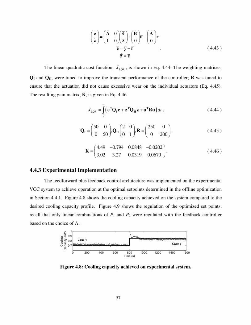
57

0=

00 0

+ +

= −

=

ee BA Au r

zz I

e y r

z e

ɶ ɶɺ ɶ

ɺ

ɺ

. ( 4.43 )

The linear quadratic cost function, , is shown in Eq. 4.44. The weighting matrices,

QI and QII, were tuned to improve the transient performance of the controller; R was tuned to

ensure that the actuation did not cause excessive wear on the individual actuators (Eq. 4.45).

The resulting gain matrix, K, is given in Eq. 4.46.

( )LQR

0

=J dt

∞

+ +∫T T T

I IIe Q e z Q z u Ru . ( 4.44 )

50 0 2 0 250 0

= , , =0 50 0 1 0 200

I IIQ Q R . ( 4.45 )

4.49 0.794 0.0848 0.0202

3.02 3.27 0.0319 0.0670K

− − =

. ( 4.46 )

4.4.3 Experimental Implementation

The feedforward plus feedback control architecture was implemented on the experimental

VCC system to achieve operation at the optimal setpoints determined in the offline optimization

in Section 4.4.1. Figure 4.8 shows the cooling capacity achieved on the system compared to the

desired cooling capacity profile. Figure 4.9 shows the regulation of the optimized set points;

recall that only linear combinations of P1 and P2 were regulated with the feedback controller

based on the choice of Λ.

Figure 4.8: Cooling capacity achieved on experimental system.

LQRJ

0 200 400 600 800 1000 1200 1400 1600

0.7

0.8

0.9

1

Co

olin

g

Ca

pa

city (

kW

)

Time (s)

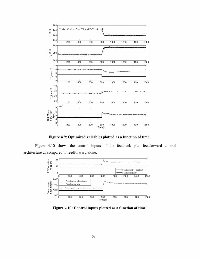
58

Figure 4.9: Optimized variables plotted as a function of time.

Figure 4.10 shows the control inputs of the feedback plus feedforward control

architecture as compared to feedforward alone.

Figure 4.10: Control inputs plotted as a function of time.

0 200 400 600 800 1000 1200 1400 1600220

240

260

280

P1 (

kP

a)

0 200 400 600 800 1000 1200 1400 1600800

850

900

P2 (

kP

a)

0 200 400 600 800 1000 1200 1400 1600-5

0

5

10

15

T1 (

de

g C

)

0 200 400 600 800 1000 1200 1400 160025

30

35

40

T3 (

de

g C

)

0 200 400 600 800 1000 1200 1400 16003

4

5

6

7x 10

-3

Re

f. M

ass

Flo

w R

ate

(k

g/s

)

Time(s)

0 200 400 600 800 1000 1200 1400 1600

5

10

15

EE

V A

pe

rtu

re

(% o

pe

n)

0 200 400 600 800 1000 1200 1400 1600500

1000

1500

2000

Time(s)

Co

mp

resso

r S

pe

ed

(rp

m)

Feedforward + Feedback

Feedforward only

Feedforward + Feedback

Feedforward only

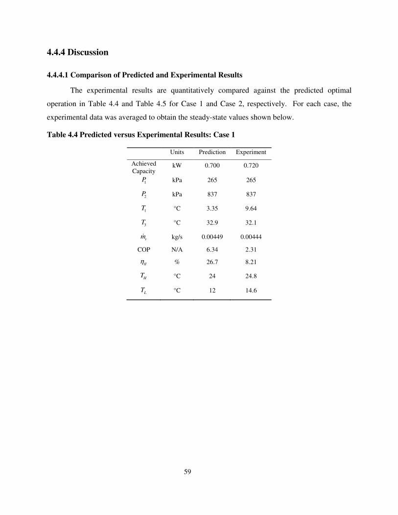
59

4.4.4 Discussion

4.4.4.1 Comparison of Predicted and Experimental Results

The experimental results are quantitatively compared against the predicted optimal

operation in Table 4.4 and Table 4.5 for Case 1 and Case 2, respectively. For each case, the

experimental data was averaged to obtain the steady-state values shown below.

Table 4.4 Predicted versus Experimental Results: Case 1

Units Prediction Experiment

Achieved

Capacity kW 0.700 0.720

1P kPa 265 265

2P kPa 837 837

1T °C 3.35 9.64

3T

°C 32.9 32.1

rmɺ kg/s 0.00449 0.00444

COP N/A 6.34 2.31

IIη

% 26.7 8.21

HT

°C 24 24.8

LT

°C 12 14.6

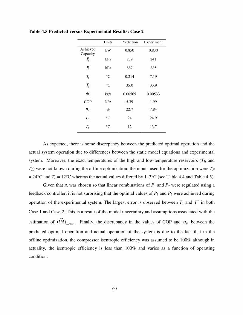
60

Table 4.5 Predicted versus Experimental Results: Case 2

Units Prediction Experiment

Achieved

Capacity kW 0.850 0.830

1P kPa 239 241

2P kPa 887 885

1T °C 0.214 7.19

3T °C 35.0 33.9

rmɺ kg/s 0.00565 0.00533

COP N/A 5.39 1.99

IIη

% 22.7 7.84

HT

°C 24 24.9

LT

°C 12 13.7

As expected, there is some discrepancy between the predicted optimal operation and the

actual system operation due to differences between the static model equations and experimental

system. Moreover, the exact temperatures of the high and low-temperature reservoirs (TH and

TL) were not known during the offline optimization; the inputs used for the optimization were TH

= 24°C and TL = 12°C whereas the actual values differed by 1‒3°C (see Table 4.4 and Table 4.5).

Given that Λ was chosen so that linear combinations of P1 and P2 were regulated using a

feedback controller, it is not surprising that the optimal values of P1 and P2 were achieved during

operation of the experimental system. The largest error is observed between T1 and *

1T in both

Case 1 and Case 2. This is a result of the model uncertainty and assumptions associated with the

estimation of � ,( )L max

UA . Finally, the discrepancy in the values of COP and IIη between the

predicted optimal operation and actual operation of the system is due to the fact that in the

offline optimization, the compressor isentropic efficiency was assumed to be 100% although in

actuality, the isentropic efficiency is less than 100% and varies as a function of operating

condition.

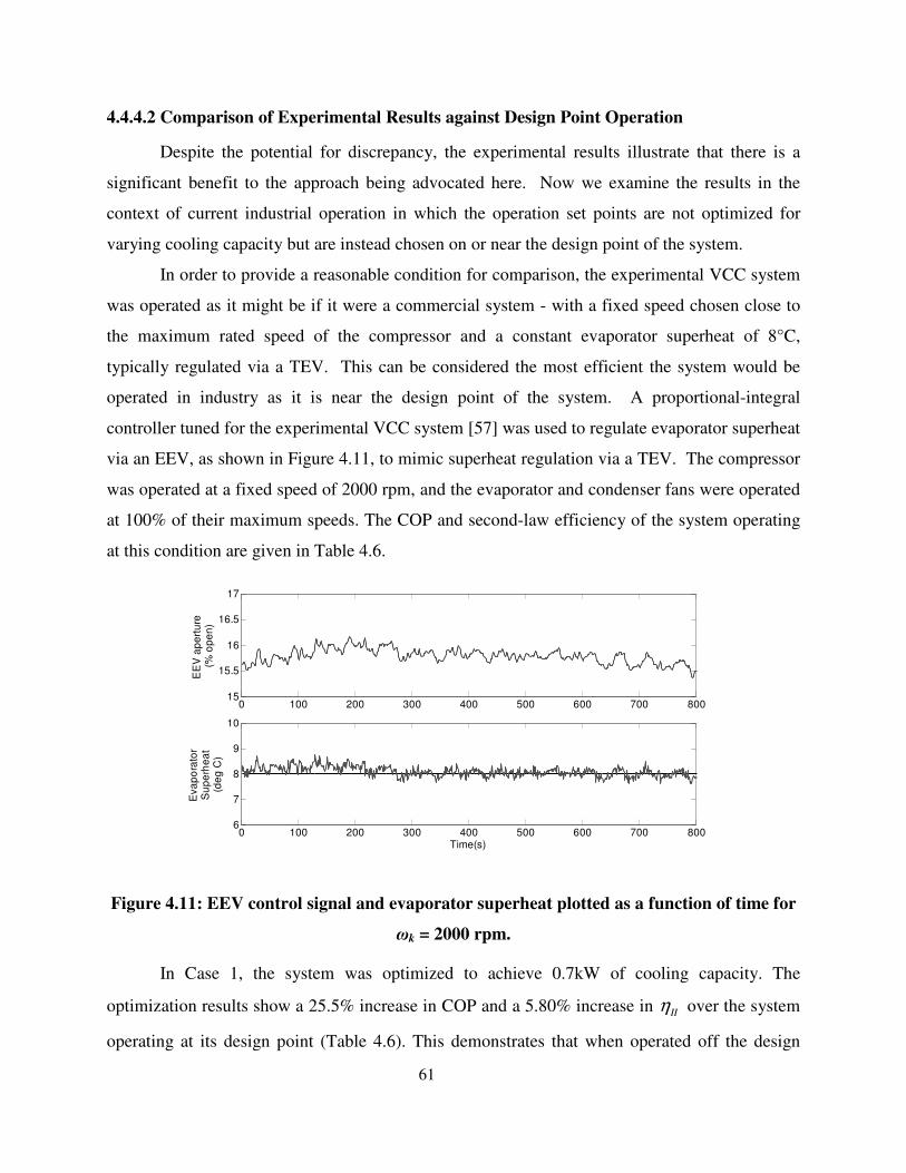
61

4.4.4.2 Comparison of Experimental Results against Design Point Operation

Despite the potential for discrepancy, the experimental results illustrate that there is a

significant benefit to the approach being advocated here. Now we examine the results in the

context of current industrial operation in which the operation set points are not optimized for

varying cooling capacity but are instead chosen on or near the design point of the system.

In order to provide a reasonable condition for comparison, the experimental VCC system

was operated as it might be if it were a commercial system - with a fixed speed chosen close to

the maximum rated speed of the compressor and a constant evaporator superheat of 8°C,

typically regulated via a TEV. This can be considered the most efficient the system would be

operated in industry as it is near the design point of the system. A proportional-integral

controller tuned for the experimental VCC system [57] was used to regulate evaporator superheat

via an EEV, as shown in Figure 4.11, to mimic superheat regulation via a TEV. The compressor

was operated at a fixed speed of 2000 rpm, and the evaporator and condenser fans were operated

at 100% of their maximum speeds. The COP and second-law efficiency of the system operating

at this condition are given in Table 4.6.

Figure 4.11: EEV control signal and evaporator superheat plotted as a function of time for

ωk = 2000 rpm.

In Case 1, the system was optimized to achieve 0.7kW of cooling capacity. The

optimization results show a 25.5% increase in COP and a 5.80% increase in IIη over the system

operating at its design point (Table 4.6). This demonstrates that when operated off the design

0 100 200 300 400 500 600 700 80015

15.5

16

16.5

17

EE

V a

pe

rtu

re

(% o

pe

n)

0 100 200 300 400 500 600 700 8006

7

8

9

10

Time(s)

Eva

po

rato

r S

up

erh

ea

t (d

eg

C)

62

point, the system achieved a higher system efficiency with the use of optimized operation

setpoints and flexible system control.

Table 4.6 Comparison of Optimization Case 1 with Design Point Operation

Parameter Units Design Point Case 1 % Improvement

Achieved

Capacity kW 0.981 0.720 --

COP

N/A 1.84 2.31 25.5

IIη % 7.76 8.21 5.80

TH

°C 24.9 24.8 --

TL

°C 12.8 14.6 --

In Case 2, the system was optimized to achieve 0.85 kW of cooling capacity, thereby

operating closer to the design point of the system. Table 4.7 shows that when operated at

optimized setpoints, an 8.15% increase in COP and a 1.03% increase in IIη were achieved.

Therefore, even as the operation of the system approached the design point operating capacity,

the optimized setpoints in conjunction with the feedforward plus feedback control scheme

enabled more efficient operation of the system. However, as evidenced by the results in the two

cases, the benefits are greater with greater deviation from the design point.

Table 4.7 Comparison of Optimization Case 2 with Design Point Operation

Parameter Units Design Point Case 2 % Improvement

Achieved

Capacity kW 0.981 0.830 --

COP

N/A 1.84 1.99 8.15

IIη % 7.76 7.84 1.03

TH

°C 24.9 24.9 --

TL

°C 12.8 13.7 --

These results highlight that optimization at the design stage alone is insufficient to ensure

efficient operation of VCC systems. A particular feature of the exergy-based objective function

is that it explicitly accounts for TH and TL, parameters that are often variable during system

operation. Regardless of how optimally a system is designed to provide a given amount of

cooling, conventional system design can only account for nominal values of TH and TL at best.

63

On the other hand, an optimization of the system that monitors environmental conditions and

adjusts system operation will likely lead to more efficient operation.

Finally, it is important to recognize the role of control in achieving efficiency

improvements during VCC system operation. The optimal operation setpoints can only be

achieved through regulation of the optimized variables, highlighting a fundamental tradeoff in

the control of VCC systems. While adding a variable frequency drive (VFD) to the compressor

and fans, and/or replacing a TEV with an EEV, requires an initial monetary investment, an

improvement in efficiency is then achievable. These results quantify, for steady-state operation,

an increase in COP that is achievable in the case of multivariable control of the VCC via a

variable-speed compressor and EEV. The results also provide concrete motivation for further

research in developing optimization and control strategies which specifically utilize all available

DOFs of the VCC.

64

Chapter 5

Optimal Control of a VCC System using EDM

In this chapter, exergy destruction minimization will be used to optimize the control

inputs for a VCC system in an optimal control framework. First, a dynamic expression for the

exergy destruction rate in a standard VCC system will be derived. Next, a finite-horizon optimal

control problem is solved to determine the control input sequences which minimize the total

exergy destroyed over the specified time horizon while tracking a desired cooling capacity

reference trajectory. The results are compared to an energy consumption minimization over the

same time horizon and highlight that the EDM chooses to actuate the system so as to consume

more energy, but operate the system with significantly higher exergetic efficiency, than the

energy consumption minimization.

5.1 Dynamic Modeling of VCC Systems

In order to use EDM with an optimal control algorithm, such as model predictive control,

it is necessary to have a dynamic model of the system to be optimized. In a four component

VCC system (compressor, condenser, expansion device, and evaporator), the compressor and

expansion device are typically modeled statically because their dynamics are significantly faster

than the dynamics of the heat exchangers. For dynamic modeling of the heat exchangers, two

different approaches have been primarily used: a finite-volume approach and a lumped parameter

moving boundary approach. Although commercial modeling packages such as e-Thermal [58],

Modelica [59], and SINDA/FLUENT [60] use a discretized modeling approach for detailed and

accurate models, this is done at the expense of model complexity, resulting in models that are not

suitable for control design. In the lumped parameter moving boundary modeling approach, the

heat exchanger is modeled with a fixed number of fluid regions (defined by fluid phase), and the

65

location of the boundary between each fluid region is a dynamic variable, allowing the length of

the fluid regions to vary. Fluid properties such as temperature, density, etc., are lumped in each

region, and an average is used for model computations. Although this approach results in some

loss in accuracy, the resulting models are of low dynamic order, making them very well suited

for control design. A review of the literature shows that this approach has been applied to a

variety of VCC systems, often with variations in the details of the modeling approach [61].

The condenser and evaporator models that are used in this chapter are described in detail

in [62] and [63]. For the purpose of control design in Section 5.3, the nonlinear models are

linearized; see Appendix C for details.

5.2 Derivation of Dynamic Rate of Exergy Destruction

To develop a dynamic expression for the total rate of exergy destruction in a standard

VCC system, it is necessary to consider each component individually as a control volume, as

shown in Figure 5.1 . The total rate of exergy destruction in the VCC system (assuming a four-

component system) is a sum of the rates of exergy destruction in each individual component:

, , , , ,dest VCC dest k dest v dest c dest eX X X X X= + + +ɺ ɺ ɺ ɺ ɺ . ( 5.1 )

Note that the evaporator and condenser fans are not considered in this analysis for the purpose of

illustrative clarity. They could be added if needed, but the refrigerant-focused construct here is

sufficient for illustrating the primary contributions of the EDM approach.

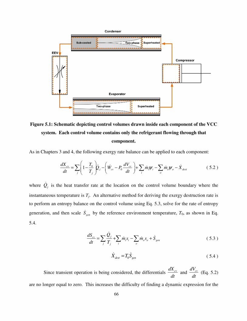
66

Figure 5.1: Schematic depicting control volumes drawn inside each component of the VCC

system. Each control volume contains only the refrigerant flowing through that

component.

As in Chapters 3 and 4, the following exergy rate balance can be applied to each component:

001cv cv

j o o dest

j i oj

cv i i

dX T dVQ W P m m X

dt T dtψ ψ

= − − − + − − ∑ ∑ ∑ɺ ɺ ɺɺ ɺ ( 5.2 )

where jQɺ is the heat transfer rate at the location on the control volume boundary where the

instantaneous temperature is Tj. An alternative method for deriving the exergy destruction rate is

to perform an entropy balance on the control volume using Eq. 5.3, solve for the rate of entropy

generation, and then scale gen

Sɺ by the reference environment temperature, T0, as shown in Eq.

5.4.

jcv

i i gen

i o

o

j

o

j

QdSm s m s S

dt T= + − +∑ ∑ ∑

ɺɺɺ ɺ ( 5.3 )

0dest genX T S= ɺɺ ( 5.4 )

Since transient operation is being considered, the differentials cvdX

dt and cvdV

dt (Eq. 5.2)

are no longer equal to zero. This increases the difficulty of finding a dynamic expression for the

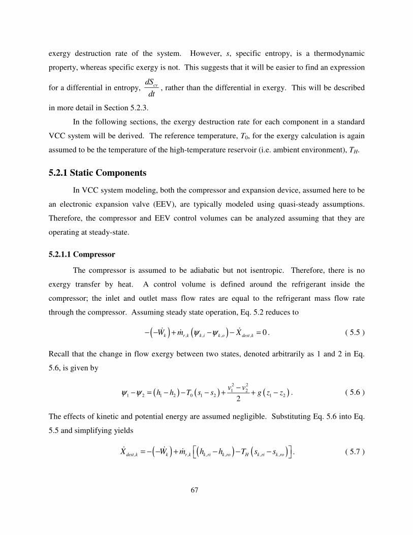
67

exergy destruction rate of the system. However, s, specific entropy, is a thermodynamic

property, whereas specific exergy is not. This suggests that it will be easier to find an expression

for a differential in entropy, cvdS

dt, rather than the differential in exergy. This will be described

in more detail in Section 5.2.3.

In the following sections, the exergy destruction rate for each component in a standard

VCC system will be derived. The reference temperature, T0, for the exergy calculation is again

assumed to be the temperature of the high-temperature reservoir (i.e. ambient environment), TH.

5.2.1 Static Components

In VCC system modeling, both the compressor and expansion device, assumed here to be

an electronic expansion valve (EEV), are typically modeled using quasi-steady assumptions.

Therefore, the compressor and EEV control volumes can be analyzed assuming that they are

operating at steady-state.

5.2.1.1 Compressor

The compressor is assumed to be adiabatic but not isentropic. Therefore, there is no

exergy transfer by heat. A control volume is defined around the refrigerant inside the

compressor; the inlet and outlet mass flow rates are equal to the refrigerant mass flow rate

through the compressor. Assuming steady state operation, Eq. 5.2 reduces to

( ) ( ), , , , 0k ik k o estr k d k

W m Xψ ψ− − + − − =ɺ ɺɺ . ( 5.5 )

Recall that the change in flow exergy between two states, denoted arbitrarily as 1 and 2 in Eq.

5.6, is given by

( ) ( ) ( )2 2

1 21 2 1 2 0 1 2 1 2

2

v vh h T s s g z zψ ψ

−− = − − − + + − . ( 5.6 )

The effects of kinetic and potential energy are assumed negligible. Substituting Eq. 5.6 into Eq.

5.5 and simplifying yields

( ) ( ) ( ), ,, , , ,dest k k ri k ro H kk r k ri k roX W m h h T s s = − − + − − − ɺ ɺ ɺ . ( 5.7 )

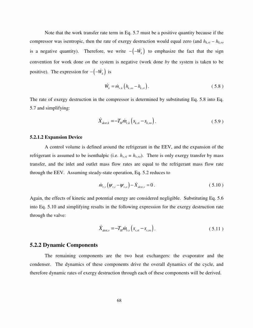
68

Note that the work transfer rate term in Eq. 5.7 must be a positive quantity because if the

compressor was isentropic, then the rate of exergy destruction would equal zero (and hk,ri – hk,ro

is a negative quantity). Therefore, we write ( )kW− − ɺ to emphasize the fact that the sign

convention for work done on the system is negative (work done by the system is taken to be

positive). The expression for ( )kW− − ɺ is

( ), , ,k ror rk k ikW m h h−=ɺ ɺ . ( 5.8 )

The rate of exergy destruction in the compressor is determined by substituting Eq. 5.8 into Eq.

5.7 and simplifying:

( ), , ,,r kdest k H k ri k roX T m s s= − −ɺ ɺ . ( 5.9 )

5.2.1.2 Expansion Device

A control volume is defined around the refrigerant in the EEV, and the expansion of the

refrigerant is assumed to be isenthalpic (i.e. hv,ri = hv,ro). There is only exergy transfer by mass

transfer, and the inlet and outlet mass flow rates are equal to the refrigerant mass flow rate

through the EEV. Assuming steady-state operation, Eq. 5.2 reduces to

( ), , ,, 0v i v o desr v t v

m Xψ ψ− − =ɺɺ . ( 5.10 )

Again, the effects of kinetic and potential energy are considered negligible. Substituting Eq. 5.6

into Eq. 5.10 and simplifying results in the following expression for the exergy destruction rate

through the valve:

( ), , ,,r vdest v H v ri v roX T m s s= − −ɺ ɺ . ( 5.11 )

5.2.2 Dynamic Components

The remaining components are the two heat exchangers: the evaporator and the

condenser. The dynamics of these components drive the overall dynamics of the cycle, and

therefore dynamic rates of exergy destruction through each of these components will be derived.

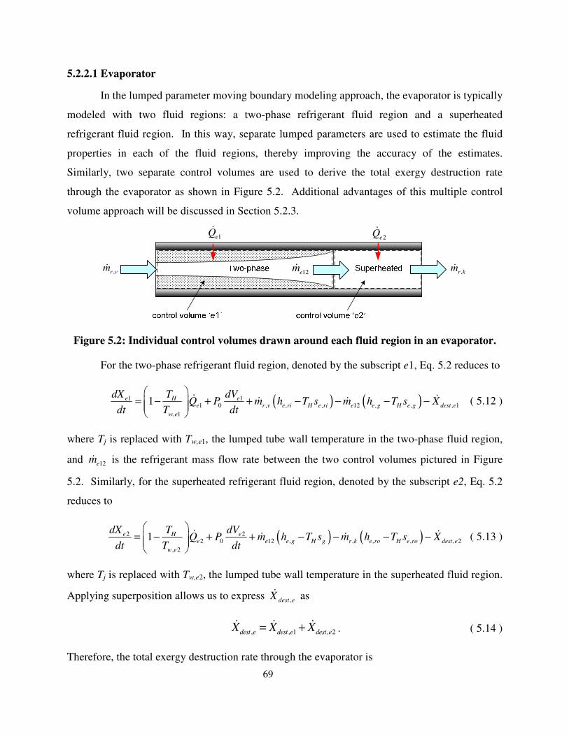
69

5.2.2.1 Evaporator

In the lumped parameter moving boundary modeling approach, the evaporator is typically

modeled with two fluid regions: a two-phase refrigerant fluid region and a superheated

refrigerant fluid region. In this way, separate lumped parameters are used to estimate the fluid

properties in each of the fluid regions, thereby improving the accuracy of the estimates.

Similarly, two separate control volumes are used to derive the total exergy destruction rate

through the evaporator as shown in Figure 5.2. Additional advantages of this multiple control

volume approach will be discussed in Section 5.2.3.

Figure 5.2: Individual control volumes drawn around each fluid region in an evaporator.

For the two-phase refrigerant fluid region, denoted by the subscript e1, Eq. 5.2 reduces to

( ) ( )1,

11 0 , , 12 , , , 1

, 1

1e

r v

eHe e ri e ri e e g e g destH H e

w e

dXT s

dVTQ P m h h X

T dm T s

tdt=

− + + − − −

−ɺ ɺ ɺɺ ( 5.12 )

where Tj is replaced with Tw,e1, the lumped tube wall temperature in the two-phase fluid region,

and 12emɺ is the refrigerant mass flow rate between the two control volumes pictured in Figure

5.2. Similarly, for the superheated refrigerant fluid region, denoted by the subscript e2, Eq. 5.2

reduces to

( ) ( )22 0 , ,

212 , , , 2

, 2

1e

e H

eHe e g g r k e ro e ro dest e

w e

H

dVTQ P m h h X

T d

dXT s m T s

d tt

− + + − −

= − −

ɺɺɺ ɺ ( 5.13 )

where Tj is replaced with Tw,e2, the lumped tube wall temperature in the superheated fluid region.

Applying superposition allows us to express ,dest eXɺ as

, , 1 , 2dest e dest e dest eX X X= +ɺ ɺ ɺ . ( 5.14 )

Therefore, the total exergy destruction rate through the evaporator is

,ɺ

r vm,ɺ

r km

1eQɺ

12emɺ

2eQɺ

70

( )

( )

1 2, 1 2 0 , , ,

, 1 , 2

,1

, ,2

1 1 e eH Hdest e e e r v e ri e ri

w e w e

r k e ro e ro

H

e eH

dV dVT TX Q Q P m h

T T dt dt

h

T s

dX dXm T s

dt dt

− + − + + +

= −

− +

− −

ɺ

ɺ

ɺɺ ɺ

( 5.15 )

where it is assumed that

( ) ( ) ( ) ( )

1 2

, 1 , 1 , 2 , 21 2.

e e e

w e r e w e r ee eUA T T UA T T

Q Q Q= +

= − + −

ɺ ɺ ɺ

( 5.16 )

In other words, it is assumed that there is no heat transfer between the refrigerant in control

volume e1 and the refrigerant in control volume e2. In Eq. 5.16, Tr,e1 and Tr,e2 refer to the

lumped refrigerant temperature in each fluid region, and (UA)e1 and (UA)e2 are the overall heat

transfer coefficients between the refrigerant and tube wall in each fluid region.

As described earlier in this chapter, it is difficult to evaluate cvdX

dt. Fortunately, the

entropy rate balance (Eq. 5.3) can be used to derive an expression for the exergy destruction rate

in terms of cvdS

dt instead of cvdX

dt. Applying Eq. 5.3 to each control volume of the evaporator

yields

( )1 1, 12 ,

, 1

, , 1,e eer v gri e e g en

w

e

e

QdSs m S

dtm s

T= + − + ɺɺ

ɺ ɺ ( 5.17 )

( )2 212 , , , 2,

, 2

,e ee e g r k e ro

w e

gen e

dSs m S

Qm s

dt T= + − +ɺ

ɺ ɺɺ ( 5.18 )

where

, , 1 , 2gen e gen e gen eS S S= +ɺ ɺ ɺ . ( 5.19 )

Substituting Eq. 5.17 and Eq. 5.18 into Eq. 5.19 and rearranging yields the following alternative

expression for the exergy destruction rate in the evaporator:

( )1 2 1 2, ,

, 1 ,

,

2

, , ,e e e e

e ri e ro

w e w e

dest e H gen e H r v H r k H H

dS dSX T S T s m T

dt d

Q Qm T T s

T tT

+ − − +

= =

− +

ɺɺ

ɺɺ ɺ

ɺ.( 5.20 )

71

Furthermore, the equivalence between the two approaches for deriving ,dest eXɺ can be verified by

setting Eq. 5.20 equal to Eq. 5.15. This yields

( )1 2 1 21 2 ,, ,

1 20 ,

e e e

e e e ee e e ri e ro

e er v r k H

dX dE

dt

dS

dt dt

Q Q P mdX dX dV dV dS dS

h m Tdt dt dt dt dt d

ht

+ +

+ = + +

+ − −

ɺ

��

ɺ ɺ ɺ

��

( 5.21 )

which is the definition of exergy (recall Eq. 2.12.1). Expressions for 1edS

dt and 2edS

dt will be

derived in Section 5.2.3.

5.2.2.2 Condenser

In the lumped parameter moving boundary modeling approach, the condenser is typically

modeled with 3 refrigerant fluid regions: a superheated fluid region, a two-phase fluid region,

and a subcooled fluid region. Therefore, separate lumped parameters are used to estimate the

fluid properties in each of the fluid regions, thereby improving the accuracy of the estimates. To

remain consistent with the modeling approach, three separate control volumes are used to derive

the total exergy destruction rate through the condenser as shown in Figure 5.3.

Figure 5.3: Individual control volumes drawn around each fluid region in a condenser.

Although at steady-state it can be assumed that the heat transfer out of the condenser is

occurring at the reference temperature, TH, the control volumes defined in Figure 5.3 for the

condenser only contain the refrigerant flowing through the condenser tube. Therefore, the

transfer of heat away from the refrigerant is occurring at the tube wall temperatures of each fluid

region.

For the superheated refrigerant fluid region, denoted by the subscript c1, Eq. 5.2 reduces

to

,r vmɺ

,r kmɺ

1cQɺ

12cmɺ 23cmɺ2c

Qɺ 3cQɺ

72

( ) ( ) ( )1,

11 0 , , , ,12 , 1

, 1

1cr k H

cHc c ri c ri c g c g dest cH

w

c

c

dXT s

dVTQ P m h h X

T dtm T s

dt=

− − + + − −

− −ɺ ɺ ɺɺ .( 5.22 )

Similarly, for the two-phase refrigerant fluid region, denoted by the subscript c2, Eq. 5.2 reduces

to

( ) ( ) ( )212 2

22 0 , , , , , 2

,

3

2

1cc H

cHc c g c g c l c l des

w c

H tc c

dXT s

dVTQ P m h h X

T dtm T s

dt=

− − + + − − −

−

ɺ ɺ ɺ ɺ .( 5.23 )

Finally, for the subcooled refrigerant fluid region, denoted by the subscript c3, Eq. 5.2 reduces to

( ) ( )

( )

323

33 0 , ,

, 3

, , , , 3

1

.

cHc c l c l

w c

r v c ro c ro des

c

c

c

H

H t

dVTQ P m h

dXT s

dt

m T

T dt

h Xs

− − + +

= −

−− −ɺ

ɺ ɺ

ɺ

( 5.24 )

As in the case of the evaporator,

, , 1 , 2 , 3dest c dest c dest c dest cX X X X= + +ɺ ɺ ɺ ɺ . ( 5.25 )

Therefore, the total exergy destruction rate through the condenser is

( ) ( ) ( )

( ) ( )

, 1 2 3

, 1 , 2 , 3

1 2 3

1 2 3

0 , , , , , ,

1 1 1

.

H H Hdest c c c c

w c w c w c

c c cr k c ri c rH H

c c

i r v c ro c o

c

rT s m T s

dX dX dX

dt dt d

T T TX Q Q Q

T T T

dV dV dVP m h h

dt dt d

t

t

− − + − − + − −

+ + + + −

=

− −

− + +

ɺ ɺ ɺɺ

ɺ ɺ ( 5.26 )

The entropy rate balance shown in Eq. 5.3 can again be applied to each control volume in

the condenser:

1 1,, , 112 ,

, 1

c cc ri c c g

w

r k g n

c

e c

QdSs m S

dt Tm s

− = + − +

ɺɺɺ ɺ , ( 5.27 )

2 212 , , 2

, 2

23 , gc c

c en c

w c

c g c c l

dSs

Qm s

Tm S

dt = + −

−+ ɺɺ

ɺɺ , ( 5.28 )

and

73

3 323 ,

,

, , , 3

3

c cc c l r v gc ro en c

w c

Qm s

dSs m S

dt T = + − +

−ɺɺ

ɺɺ ( 5.29 )

where

, , 1 , 2 , 3gen c gen c gen c gen cS S S S= + +ɺ ɺ ɺ ɺ . ( 5.30 )

Substituting Eqs. 5.27 – 5.29 into Eq. 5.30 and rearranging yields the following alternative

expression for the exergy destruction rate in the condenser:

( )1 2 3, ,, , , ,

, 1 , 2

1 2 3

, 3

c ri c roc c c

dest c H gen c H

c c c

r k H r v H

w c w c w c

H

Q Q QX T S T s m

T T Tm T T

dS

s

dS dST

dt dt dt

− −

+

= = +

+ +

+

ɺ ɺ ɺɺɺ ɺ ɺ

( 5.31 )

where it is assumed that

1 2 3cc c cQ Q Q Q= + +ɺ ɺ ɺ ɺ . ( 5.32 )

Again, Eq. 5.32 relies on the assumption that there is no heat transfer between the refrigerant in

control volumes c1, c2, and c3.

Expressions for cidS

dt, i={1,2,3}, will be derived in the next section.

5.2.3 Evaluating the Entropy Differential

In order to express cvdS

dt in terms of thermodynamic variables, the method proposed in

[64], described in Eqs. 5.33 – 5.36, is used.

{ } { } { }

( 1, 2) ( 1, 2)

cv cv

cv cv c

cv

v

dS dm dsdm s var var s var var m

dt dt dt dt= = + ( 5.33 )

( ) ( ) ( 1) ( 2)

( 1) ( 2)

cv cv cvds s sd var d var

dt var dt var dt

∂ ∂ = +

∂ ∂ ( 5.34 )

{ } ( ) ( )

( , )

cv cv cv

hP

ds s sd dh dPs h P

dt dt h dt P dt

∂ ∂= = +

∂ ∂ ( 5.35 )

74

( ) ( )

cv cv cv cv

c

P

v cv

h

dS dm s sdh dPs m

dt dt h dt P dt

∂ ∂= + +

∂ ∂

( 5.36 )

In Eq. 5.35 the dependent variables were chosen as specific enthalpy and pressure, but they can

be chosen as any two independent thermodynamic state variables. Equation 5.36 highlights why

it is helpful to define multiple control volumes for the heat exchangers in which a separate

control volume is drawn around each fluid region (recall Figure 5.2). This formulation allows

for lumped parameters to be used to approximate scv and mcv for each control volume as is done

in the lumped parameter moving boundary dynamic modeling approach.

The expression for cvdm

dt can be derived in the lumped parameter moving boundary

framework for each control volume as described in [65].

5.2.3.1 Entropy Rate of Change in Evaporator

For the two-phase fluid region of the evaporator, refrigerant mean void fraction, rather

than specific enthalpy, and pressure will be used to describe specific entropy. Mean void

fraction is related to mean quality, x , by the following relationship:

g

xρ

γρ

= . ( 5.37 )

Evaluating Eq. 5.36 for the two-phase fluid region of the evaporator yields

1 1 1 11 1

( ) ( )

e e

e eP

e e e e

e e

dS dm s d s dPs m

dt dt dt P dtγ

γ

γ

∂ ∂= + +

∂ ∂

( 5.38 )

which can be further simplified as

1 1 11 1 ,

11 ,

( ) ( )

e e

e e CR e

e eP

e e e e

e R e

dS dm s d s dPs L A

dt dt dt P dtγ

γρ ζ

γ

∂ ∂

=∂ ∂

+ + ( 5.39 )

where

( )1 1, 12 1 , ,

e er v e e CR e R e

dm dm m A L

dt dt

ζρ= − +ɺ ɺ ( 5.40 )

and

75

( )( )( )

, ,, ,

,

,1

,

,

11 .

1

e l e l

e l

e l

e e g e g e

e e e g e

e e g e

s ss x s x s

γ ρ γ ρ

γ ρ γ ρ

+ −= + − =

+ − ( 5.41 )

The variables ,e l

ρ , ,e g

ρ , ,e l

s , and ,e g

s are all solely functions of pressure. The partial derivatives

1

e P

es

γ

∂

∂ and 1

e

es

Pγ

∂

∂, shown in Eq. 5.42 and Eq. 5.43 respectively, are derived using Eq. 5.41.

( )( )( ) ( )( )( )

( )( ), , , , ,1

,

, , , , , , ,

2

,

1 1

1

e e g e e g e g e l e e g e g e e g

e P e e g e

e l e l e l e l e le

e l

s s s ss γ ρ γ ρ ρ ρ γ ρ γ ρ ρ ρ

γ γ ρ γ ρ

+ − − − + − −∂=

∂ + − ( 5.42 )

1 2

3

1

e

e

s

Pγ

β β

β

∂ −=

∂ ( 5.43 )

( )( ) ( ) ( )

( )( ) ( )

( )( )

, ,

, , ,

,

, ,

,

, ,

1 , , ,

,

2 , ,

2

3 ,

1 1 1

1 1

1

e g e g

e e g e e e g e g e e e

e e e e

e g

e e g e g e

e l e l

e l e l e l

e l

e l e e

e

e l

e l

e

e e g e

ds d ds ds s

dP dP dP dP

d ds s

dP dP

ρ ρβ γ ρ γ ρ γ ρ γ γ ρ γ

ρ ρβ γ ρ γ ρ γ γ

β γ ρ γ ρ

= + − + + − + −

= + − + −

= + −

( 5.44 )

Evaluating Eq. 5.36 for the superheated fluid region of the evaporator yields

2 22 22 2 2

2,

2

,

( ) ( )

e e e

e e e CR

e e e

e e

P

R

e e h

dS dm s dh s dPs L A

dt dt h dt P dtρ ζ

∂= +

∂ ∂

∂+ ( 5.45 )

where

( )2 1,12 , , , .

e r k ge e

CR e Re e

dm dm m A L

dt dt

ζρ= − +ɺ ɺ ( 5.46 )

5.2.3.2 Entropy Rate of Change in Condenser

The procedure described in the previous section can be applied to the rate of change of

entropy in each of the condenser control volumes. It is assumed that the outlet refrigerant

condition of the condenser is subcooled liquid; therefore, the condenser is characterized using

three fluid regions. As in the case of the evaporator, specific enthalpy and pressure are used to

describe specific entropy in the superheated and subcooled fluid regions, and mean void fraction

and pressure are used in the two-phase fluid region.

76

The expressions for 1cdS

dt, 2c

dS

dt, and 3c

dS

dt are given in Eqs. 5.47 – 5.52, respectively.

1 1 1 11 1 1 , ,

1

1 ( ) ( )

c c

c c c R c CR c

c cP

c c c c

h



∂ ∂= + +

∂ ∂

( 5.47 )

( ) 1, 12

1, ,,

cr k c CR c R c

cg c

dm dm m A L

dt dt

ζρ= − +ɺ ɺ ( 5.48 )

,2

2 2 2 , ,

,22 2( ) ( )

c cc c c R c CR c

c cP

c cc cs sdS dm d dP

s L Adt dt dt P dt

γ

γρ ζ

γ

∂ ∂= +

∂ +

∂ ( 5.49 )

( ) 1 2 1, , , ,

212 23 , ,

c c c

CR c R c C

c

c c l c g c R c R c

dm d d dm m A L A L

dt dt dt dt

ζ ζ ζρ ρ= − + +

−

ɺ ɺ ( 5.50 )

3 3 3 33 3 3 , ,

3

3 ( ) ( )

c c

c c c R c CR c

c cP

c c c c

h



∂ ∂= + +

∂ ∂

( 5.51 )

( ) 1 2, ,

323 , ,

c c

CR c R c

c

c r v l c

dm d dm m A L

dt dt dt

ζ ζρ= − +

−

ɺ ɺ ( 5.52 )

5.2.4 Dynamic Rate of Exergy Destruction for Complete VCC System

Substituting Eqs. 5.9, 5.11, 5.20, and 5.31 into Eq. 5.1 and simplifying results in

, ,dest VCCXɺ the instantaneous exergy destruction rate in the standard VCC system:

2,

1 2

1 2 3 1

, 1 , 2 , 3 1 , 2

1 3

,

2

c c c eH

w c w c

edest VCC

e

w c w e w e

c cH

e c

Q Q Q Q QT

T T T T T

dS dS d

X

S dS dST

dt dt dt dt dt

=

+ + − −

+ + + +

+

ɺ ɺ ɺ ɺ ɺɺ

( 5.53 )

where

1 1 11 1 ,

11 ,

( ) ( )

e ee e CR e

e eP

e e e ee R e

dS dm s d s dPs L A

dt dt dt P dtγ

γρ ζ

γ

∂ ∂

=∂ ∂

+ + , ( 5.54 )

2 22 22 2 2

2,

2

,

( ) ( )

e e e

e e e CR

e e e

e e

P

R

e e h



∂= +

∂ ∂

∂+ , ( 5.55 )

77

1 1 1 11 1 1 , ,

1

1 ( ) ( )

c c

c c c R c CR c

c cP

c c c c

h



∂ ∂= + +

∂ ∂

, ( 5.56 )

,2

2 2 2 , ,

,22 2( ) ( )

c cc c c R c CR c

c cP

c cc cs sdS dm d dP

s L Adt dt dt P dt

γ

γρ ζ

γ

∂ ∂= +

∂ +

∂, ( 5.57 )

and

3 3 3 33 3 3 , ,

3

3 ( ) ( )

c c

c c c R c CR c

c cP

c c c c

h



∂ ∂= + +

∂ ∂

. ( 5.58 )

5.3 Optimal Control Problem Formulation

In this section, an optimal control problem is formulated using total exergy destruction as

the minimization metric. Rather than optimizing operational setpoints as was done in Chapters 3

and 4, the decision variables in the optimal control problem formulated in this section are the

control inputs themselves. Additionally, the optimization is a dynamic one in the sense that

dynamic model information about how the system will behave at future time steps is used to

influence control decisions at the current time step.

In Section 5.3.1, model predictive control (MPC) is introduced. In Section 5.3.2, an

objective function is defined based on the dynamic exergy destruction rate derived in Section

5.2. Finally, in Section 5.3.3, the constraints enforced in the optimal control problem are

defined.

5.3.1 Model Predictive Control

There are many different optimal control algorithms. However, all of them are used to

find optimal control decisions by minimizing some objective function. Here, model predictive

control (MPC), a receding-horizon optimal control framework, will be used. MPC uses a

dynamic model to predict how a system will behave in response to a particular sequence of

control decisions over a specified prediction horizon.

The prediction horizon, np, is the number of discrete time steps over which the system

behavior is predicted. It is defined as

78

horiz

p

ont

nt

=∆

. ( 5.59 )

where t∆ is the length of the discrete time step and thorizon is the length of time over which the

algorithm predicts the system behavior. The control horizon, nu, is the number of discrete time

steps for which control decisions are optimized, where u p

n n≤ .

A linearized discrete model of the system dynamics of the form

[ ] [ ] [ ] [ ]211k k k kδ δ δ δ+ = + +x A x B u B d ( 5.60 )

is used to predict the system behavior over the prediction horizon. Since the model is linearized

about some equilibrium condition of the system, δx, δu, and δd represent deviations from the

equilibrium condition. The state, input, and disturbance vectors are described in Eqs. 5.61, 5.62,

and 5.63, respectively. Note that instead of treating the evaporator and condenser fan speeds as

the decision variables, the air mass flow rates produced by each fan, ,a emɺ and ,a c

mɺ , are the

decision variables. Details of the model linearization are provided in Appendix C. To simplify

the notation, the use of δ will be dropped since it is understood that we are discussing deviations

about some nominal operating condition when referring to state, input, and disturbance variables.

1 2 , 1 , 2 1 1 1 3 , 1 , 2 3

15

,

T

e e e w e w e e c c c c c w c w c w c cP h T P h h T T TTζ γ ζ ζ γ = ∈ x ℝ ( 5.61 )

4

, ,

T

v k a e a ca m mω = ∈ u ɺ ɺ ℝ ( 5.62 )

,

2

,

T

e ai c aiT T = ∈ d ℝ ( 5.63 )

One can constrain the rate of change in control decisions over the control horizon by

augmenting the system with additional states defined as

[ ] [ ]1k k= −ux u ( 5.64 )

where

[ ] [ ] [ ]1 .k k k= − + ∆u u u ( 5.65 )

Therefore,

79

[ ] [ ] [ ]1k k k+ = + ∆u ux x u ( 5.66 )

and the augmented state-space representation of the system is given by

[ ][ ]

[ ][ ]

[ ] [ ]1

1

k kk k

k k

+ = + ∆ +

+

1 1 2

u u

x xA B B Bu d

x x0 I I 0 ( 5.67 )

which is represented with the simplified notation shown in Eq. 5.68.

[ ] [ ] [ ] [ ]1k k k k+ = + ∆ +1 2x Ax B u B d ( 5.68 )

, , , 1 1 2

1 2

u

x A B B Bx A B B

x 0 I I 0

= =

=

( 5.69 )

For a numerical optimization, it is convenient to define the input vector in its lifted form,

[ ][ ] [ 1] .[ 1]T

uk k k n∆ = ∆ ∆ + ∆ + −U u u u⋯ ( 5.70 )

Using the lifted input vector, ∆U, and the initial value of the state vector, [0]x , the evolution of

all of the states can be quickly evaluated in the lifted vector X using the lifted matrix equation

[ ]k= + ∆ +1 2

X Tx S U S D ( 5.71 )

where

[ ] [ 1] [ .1]T

pk k k n = + + − X x x x⋯ ( 5.72 )

The expressions for T, S1, and S2 are given by

2

,

pn

=

A

AT

A

⋮ ( 5.73 )

80

1

12

11

0 0

0

,

pp

p pp

u

u

u u

n

n nn

n n n nn

−

− −−

− − −−

=

1

1

1

11 11

11

1 11

B

AB

B

BA B ABS

A BA B

A B A BA B

…

⋱ ⋱ ⋮

⋮ ⋱

⋯

⋮⋮ ⋮⋮

⋱⋱

⋯

( 5.74 )

and

1

2

12

11

0 0

0

.u

upp

p pp u u

n

n nn

n n n nn

−

− −−

− − −−

=

2

2

2

22 2

22

2 22

B

AB

B

BA B ABS

A BA B

A B A BA B

…

⋱ ⋱ ⋮

⋮ ⋱

⋯

⋮⋮ ⋮⋮

⋱⋱

⋯

( 5.75 )

The objective function JEDM,VCC, which will be defined in the next section, is a function of X .

5.3.2 Objective Function

Since the optimal control framework that will be used considers a finite time horizon, the

total exergy destroyed over the time horizon, as opposed to the exergy destruction rate at each

time instant, will be minimized. Additionally, for robustness considerations, the performance

objective of achieving a specified cooling capacity is included in the objective function rather

than as an equality constraint, and a weighting parameter, λ, is used to emphasize the importance

of one objective over the other. Finally, in order to numerically solve this type of optimization

problem, the cost function must be evaluated in discrete time. Therefore, numerical integration

will be used to approximate the total exergy destroyed over the finite time horizon.

The complete objective function is expressed as

( ), ,21

· [ ]p

EDM VCC des ach dest VCC

PerformanceObjective Efficiency

Object

k

v

n

i e

J = C C X k tλ=

− ∆

+ ∑ ɺ

��

( 5.76 )

81

where pn

desC ∈ℝ is specified in the optimization problem and ∈ℝ p

ach

nC is calculated using the

expression

( ) ( ) ( ) ( ), 1 , 1 , 2 , 21 2.

ach w e r e w ree e eeUA T T UAQ TC T = = − + −ɺ ( 5.77 )

The efficiency objective can be expanded as

( )

2

1

1 2 3 1,

, 1 , 2 , 3 , 1 , 2

1 2 1

1

2 3

1

[ ] [ ] [ ] [ ] [ ][ ]

[ ] [ ] [ ] [ ] [ ]

[ ] [ ] [ ] [ ] [ ]

p p

p

c c c edest VCC H

w c w c w

n n

e

k k

n

c c

c w e w e

H e c

k

e

Q k Q k Q k Q k Q kX k t T t

T k T k T k T k T k

T g k g k g k g k g k t

= =

=

∆ + + − − ∆

=

+ + +

+ +

∆

∑ ∑

∑

ɺ ɺ ɺ ɺ ɺɺ

( 5.78 )

where

( ) ( ), ,[ ] [ ] [· {1, 2[ ] }] , ,w ei eeii r ie

k UA k T k T iQ k ∈= −ɺ ( 5.79 )

( ) ( ), ,· {1,2[ ] [ ] [ ] , }[ 3] ,r ci w cicc ii

k UA k T k TQ ik , ∈= −ɺ ( 5.80 )

1

1 1

1

1 1

1 , 12 , , 1

1, , [ ] [ ]

[ ] [ 1][ ] [ ] [ ] [ ] [ ]

( ) [ ] [ 1] ( ) [ ] [ 1][ ] [ ] ,

e

e

e

e r v e R e CR e

e e e e e

e

R e CR e

e

e

e

e

e

s

k

k kg k k m k m k L A k

t

s k k s P k P kL A k k

t P k

t

ζ ζρ

γ γρ ζ

γ

− − = − +

∆

∂ − − ∂ − − + +

∂ ∆ ∂ ∆

ɺ ɺ

( 5.81 )

2

1 1

2 , ,

, ,

2

12 , ,

2 2 2 2

2 2[

[ ] [ 1][ ] [ ] [ ] [ ] [ ]

( ) [ ] [ 1] ( ) [ ] [ 1][ ]] [ ] [ ]

e e

e R e CR e

R e CR e

e

e e r k g e

e e e e e e

e e

e


t

s h k h k s P k P kL A k k

s

k k ,h t P t

ζ ζρ

ρ ζ

− − = − +

∆

∂ − − ∂ − − + +

∂ ∆ ∂ ∆

ɺ ɺ

( 5.82 )

1 1

1 1 , 12 , ,

1 1

, ,

,

1

1 1

1

1

[

[ ] [ 1][ ] [ ] [ ] [ ] [ ]

( ) [ ] [ 1] ( ) [ ] [ 1][] [ ] ] [ ] ,

c c

c c r k c R c CR c

c c c c

R c CR c c c

c c

g c

c c


t

s h k h k s P k P kL A k k

h t P k

t

s

k

ζ ζρ

ρ ζ

− − = − +

∆

∂ − − ∂ − − +

∂ ∆ ∂ ∆

+

ɺ ɺ

( 5.83 )

12 23

1 1 2 2

2 2 , ,

1

,

,

1

2 , ,

, 2

2

, 2

[ ] [ 1] [ ] [ 1][ ] [ ] [ ] [ ] [ ]

[ ] [ 1][ ]

[ ] [ ]

[ ]

( ) [ ] [ 1][ ]

c c c c

c c R c CR c

c c

c R c CR c

c c

R c CR c c c

c c l c

g c

c

c

k k k kg k k m k m k Ls

s

A kt t

k kk L A k

t

s k kL A k

tk k

ζ ζ ζ ζρ

ζ ζρ

γ γρ ζ

γ

− − − − = − + +

∆ ∆

− −

∆

∂ − −+

∂ ∆

−

ɺ ɺ

2( ) [ ] [ 1][ ] ,c cc

c

s P k P kk

P t

∂ − − +

∂ ∆

( 5.84 )

82

and

23 , ,

3 3

1 1 2 2

3 3 , ,

3 3

, , 3 3

3

[ ] [ 1] [ ] [ 1][ ] [ ] [ ] [ ] [ ]

( ) [ ] [ 1] ( ) [ ] [ 1[ ] [ ]

][ ] [ ]

c c c c

c c R c CR c

c c c c

R c CR c c c

c c

c r v l c

c c

k k k kg k k m k m k L A k

t t

s h k h k s P k P kL A k k .

h t P t

s

k k

ζ ζ ζ ζρ

ρ ζ

− − − − = − +

∆ ∆

∂ − − ∂

−

− − + +

∂ ∆ ∂ ∆

ɺ ɺ

( 5.85 )

For clarity of notation, the rate of change of entropy in each evaporator control volume is

denoted by the function gei where i = {1,2}. Similarly, in each condenser control volume, the

rate of change of entropy is denoted by the function gci where i = {1,2,3}. It should also be noted

that JEDM,VCC is not only a function of the states of the dynamical system representation of the

VCC system, but also a function of variables such as Tr,c1 and 2( )e

s

h

∂

∂ which are nonlinear

functions of the states. These variables are typically evaluated using data-based refrigerant look-

up tables [65].

5.3.3 Constraints

In the MPC framework, upper and lower bound constraints can easily be placed on the

values of the control decisions at each time instant. These are detailed in Section 5.4.1 for the

specific VCC system considered in the case study. Additionally, upper and/or lower bound

constraints can be enforced on specific state variables in the dynamical system. The constraints

enforced in the case study are

1

0.9[ 5]ζ ≤ ∀e

k k ( 5.86 )

and

1 2[ ] [ ] 0.95 .ζ ζ ≤ ∀+

c c k k k ( 5.87 )

Equations 5.86 and 5.87 ensure that the normalized lengths of the superheated fluid region in the

evaporator and subcooled region in the condenser, respectively, are maintained at some

minimum fraction of the total tube length in each heat exchanger. These constraints are

necessary for the purpose of this discussion since the linearized model assumes that the

evaporator is operating with 2 fluid regions and that the condenser is operating with 3 fluid

regions.

83

Finally, the following three nonlinear thermodynamic constraints are introduced to satisfy

the second law of thermodynamics:

,[ ] [ ] 0− ≥ ∀ɺ ɺdestVCC VCC

X kW k k ( 5.88 )

where ɺVCC

W is equal to the power (energy consumption rate) of the compressor, ɺk

W , and

,

,

,

,

0

0

0

0

[ ]

[ ]

[ ]

[ ] .

dest k

dest v

dest e

dest c

X k

X k

X

k

k

k

X k

k

k

≥ ∀

≥ ∀

≥ ∀

≥ ∀

ɺ

ɺ

ɺ

ɺ

( 5.89 )

Equation 5.88 ensures that the reversible power is always nonnegative, and the inequalities

shown in Eq. 5.89 ensure that the exergy destruction rate for each individual component of the

VCC system is always nonnegative.

5.4 Simulated Case Study

In this section, a case study will be presented in which the exergy destruction

minimization (EDM) optimal control problem is solved for a particular VCC system and

specified cooling capacity demand profile. In Section 5.4.1 the solution of the EDM optimal

control problem will be presented. In Section 5.4.2, a second optimal control problem

minimizing energy consumption over a finite time horizon will be formulated and solved, and

the solution will be compared against the results presented in Section 5.4.1. The tradeoffs

between minimizing energy consumption and minimizing exergy destruction will discussed,

specifically in the context of transient VCC system operation.

5.4.1 Solution of EDM Optimal Control Problem

The exergy destruction minimization (EDM) optimal control problem formulated in the

previous section is solved offline as a finite-horizon optimization problem and then validated on

the corresponding nonlinear VCC system model in the ATTMO Toolbox [66]. The function

fmincon in the MATLAB Optimization Toolbox was used with a sequential quadratic

programming algorithm to find the solution, defined as

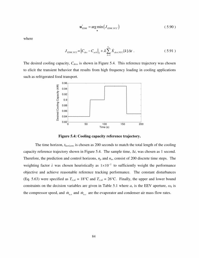
84

( )*

,arg min

u

uEDM EDM VCC

J= ( 5.90 )

where

,21

, · [ ]· .p

EDM VCC des ach

n

k

dest VCCJ = C C X k t λ

=

+− ∆∑ ɺ ( 5.91 )

The desired cooling capacity, Cdes, is shown in Figure 5.4. This reference trajectory was chosen

to elicit the transient behavior that results from high frequency loading in cooling applications

such as refrigerated food transport.

Figure 5.4: Cooling capacity reference trajectory.

The time horizon, thorizon, is chosen as 200 seconds to match the total length of the cooling

capacity reference trajectory shown in Figure 5.4. The sample time, ∆t, was chosen as 1 second.

Therefore, the prediction and control horizons, np and nu, consist of 200 discrete time steps. The

weighting factor λ was chosen heuristically as 21 10−× to sufficiently weight the performance

objective and achieve reasonable reference tracking performance. The constant disturbances

(Eq. 5.63) were specified as Te,ai = 18°C and Tc,ai = 26°C. Finally, the upper and lower bound

constraints on the decision variables are given in Table 5.1 where av is the EEV aperture, ωk is

the compressor speed, and ,a emɺ and ,a c

mɺ are the evaporator and condenser air mass flow rates.

0 50 100 150 2000.82

0.84

0.86

0.88

0.9

0.92

0.94

0.96

Time (s)

De

sire

d C

oo

ling

Ca

pa

city

(kW

)

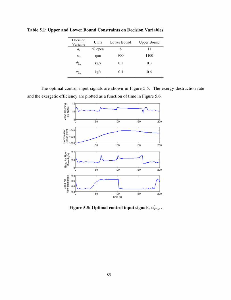
85

Table 5.1: Upper and Lower Bound Constraints on Decision Variables

Decision

Variable Units Lower Bound Upper Bound

av % open 8 11

ωk rpm 900 1100

,a emɺ kg/s 0.1 0.3

,a emɺ kg/s 0.3 0.6

The optimal control input signals are shown in Figure 5.5. The exergy destruction rate

and the exergetic efficiency are plotted as a function of time in Figure 5.6.

Figure 5.5: Optimal control input signals,

*uEDM

.

0 50 100 150 2008

10

12

Valv

e O

pe

nin

g (

% o

pe

n)

0 50 100 150 2001000

1020

1040

Co

mp

ressor

Sp

ee

d (rp

m)

0 50 100 150 2000

0.2

0.4

Eva

p A

ir F

low

R

ate

(kg

/s)

0 50 100 150 2000.2

0.4

0.6

0.8

Time (s)

Co

nd

Air

F

low

Rate

(kg

/s)

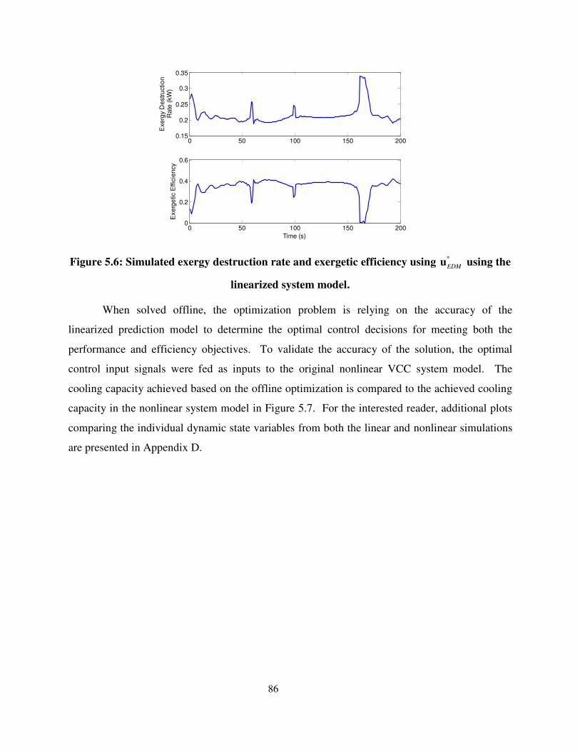
86

Figure 5.6: Simulated exergy destruction rate and exergetic efficiency using *uEDM

using the

linearized system model.

When solved offline, the optimization problem is relying on the accuracy of the

linearized prediction model to determine the optimal control decisions for meeting both the

performance and efficiency objectives. To validate the accuracy of the solution, the optimal

control input signals were fed as inputs to the original nonlinear VCC system model. The

cooling capacity achieved based on the offline optimization is compared to the achieved cooling

capacity in the nonlinear system model in Figure 5.7. For the interested reader, additional plots

comparing the individual dynamic state variables from both the linear and nonlinear simulations

are presented in Appendix D.

0 50 100 150 2000.15

0.2

0.25

0.3

0.35

Exe

rgy D

estr

uctio

n R

ate

(kW

)

0 50 100 150 2000

0.2

0.4

0.6

Time (s)

Exe

rge

tic E

ffic

ien

cy

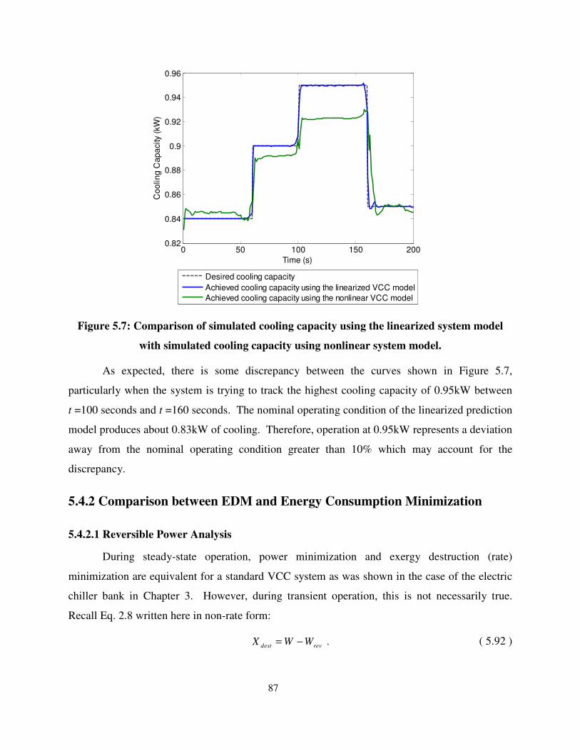
87

Figure 5.7: Comparison of simulated cooling capacity using the linearized system model

with simulated cooling capacity using nonlinear system model.

As expected, there is some discrepancy between the curves shown in Figure 5.7,

particularly when the system is trying to track the highest cooling capacity of 0.95kW between

t =100 seconds and t =160 seconds. The nominal operating condition of the linearized prediction

model produces about 0.83kW of cooling. Therefore, operation at 0.95kW represents a deviation

away from the nominal operating condition greater than 10% which may account for the

discrepancy.

5.4.2 Comparison between EDM and Energy Consumption Minimization

5.4.2.1 Reversible Power Analysis

During steady-state operation, power minimization and exergy destruction (rate)

minimization are equivalent for a standard VCC system as was shown in the case of the electric

chiller bank in Chapter 3. However, during transient operation, this is not necessarily true.

Recall Eq. 2.8 written here in non-rate form:

.dest rev

X W W = − ( 5.92 )

0 50 100 150 2000.82

0.84

0.86

0.88

0.9

0.92

0.94

0.96

Time (s)

Co

olin

g C

ap

acity (

kW

)

Desired cooling capacity

Achieved cooling capacity using the linearized VCC model

Achieved cooling capacity using the nonlinear VCC model

88

Using Eq. 5.92, the reversible work during a finite time horizon assuming transient operation of

the VCC system is

( )( )

( )

2

,

1 2 3 1

,

, 1 , 2 , 3 , 1 , 2

1

,

1 1

2 31

1

2

[ ] [ ] [ ] [ ] [ ][ ] [ ] [ ]

[ ] [ ] [ ] [ ] [ ]

[ ] [ ] [ ] [ ] [ ]

p p

p

rev dest

n n

e

k ro k ri

k k

n

c c

c c c e

r k H

w c w c w c w e w e

e e c

k

H

k k

W W X

Q Q Q Q Qm T

T T T T T

T g g g g g

k k kk h k h k

k k k k k

k k k k k

= =

=

=

= − −

−

+ + − −

+ + + +−

∑ ∑

∑

ɺ ɺ ɺ ɺ ɺɺ ( 5.93 )

which will not be constant with respect to the decision variables in the optimization problem.

Therefore, we expect that the optimal control problem formulated with a power minimization

metric will produce a different optimal solution than was presented in the previous section.

We will now define a second optimal control problem where the objective function,

JPM,VCC, is formulated to minimize the total energy consumed over the time horizon:

( )

( ) ( )

, 2

, ,2

1

1

· [ ]

· [ ] [ ] [ ]

p

p

PM VCC des ach k

des ach k k ro k r

n

i

k

n

k

J C C W k t

C C m k h k h k t

λ

λ

=

=

− ∆

= −

− ∆

= +

+

∑

∑

ɺ

ɺ

( 5.94 )

where k

Wɺ is the instantaneous power consumption (i.e. energy consumption rate) in the VCC

system. The optimal solution is defined as

( )*

,arg min .

u

uPM PM VCC

J = ( 5.95 )

Using an abuse of notation, the subscript PM, signifying power minimization, will be used to

represent energy consumption minimization, rather than using the abbreviation ECM which can

be easily confused with EDM.

The energy consumption minimization optimal control problem was formulated with the

same constraints, weighting factor λ, and constant disturbances that were specified in the optimal

control problem designed to minimize total exergy destruction. The solutions of the two optimal

control problems will be compared in the following figures. Note that all of the figures contain

simulated results using the linearized model.

First the tracking of the desired cooling capacity by each optimal controller is compared

in Figure 5.8. Both optimal solutions produce very similar results.

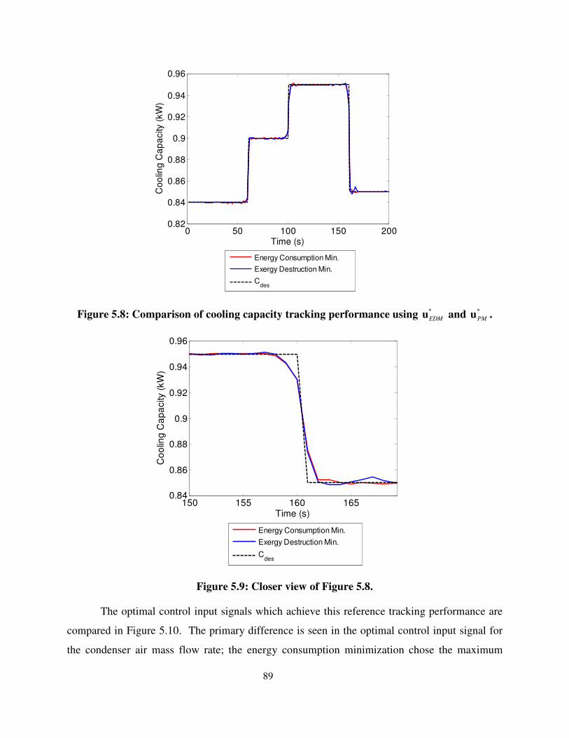
89

Figure 5.8: Comparison of cooling capacity tracking performance using *uEDM

and *uPM

.

Figure 5.9: Closer view of Figure 5.8.

The optimal control input signals which achieve this reference tracking performance are

compared in Figure 5.10. The primary difference is seen in the optimal control input signal for

the condenser air mass flow rate; the energy consumption minimization chose the maximum

0 50 100 150 2000.82

0.84

0.86

0.88

0.9

0.92

0.94

0.96

Time (s)

Co

olin

g C

ap

acity

(kW

)

Energy Consumption Min.

Exergy Destruction Min.

Cdes

150 155 160 1650.84

0.86

0.88

0.9

0.92

0.94

0.96

Time (s)

Co

olin

g C

ap

acity (

kW

)



Cdes

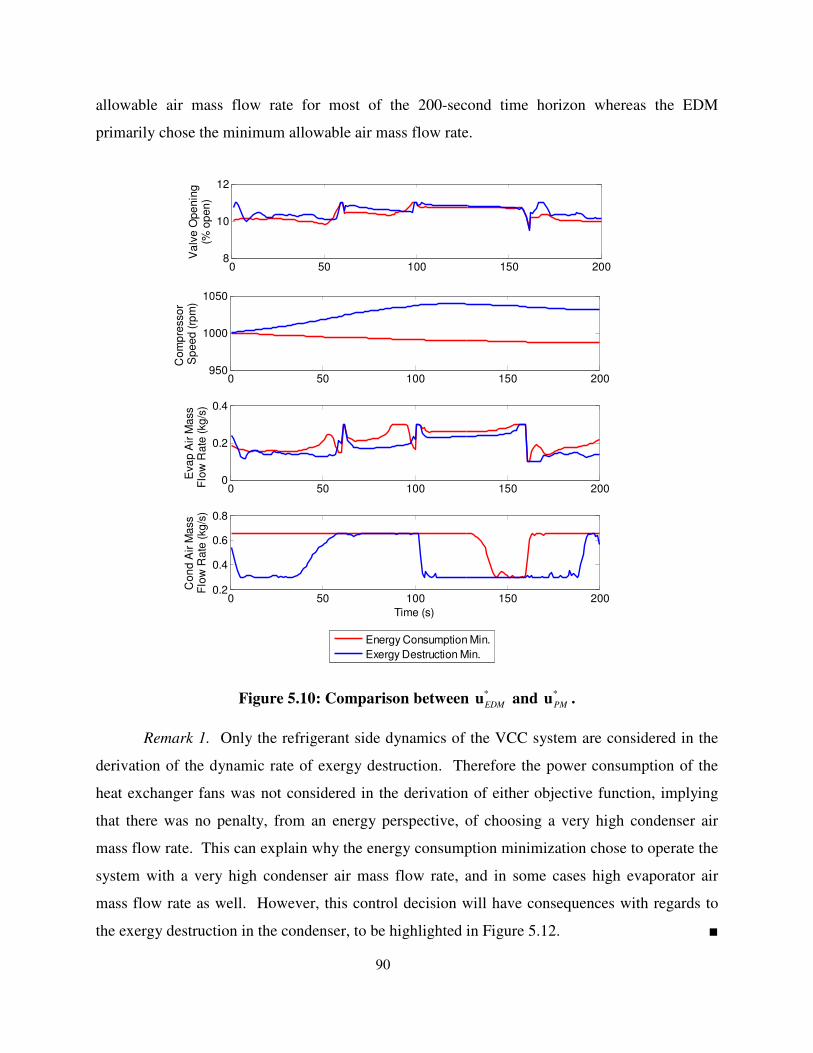
90

allowable air mass flow rate for most of the 200-second time horizon whereas the EDM

primarily chose the minimum allowable air mass flow rate.

Figure 5.10: Comparison between *uEDM

and *uPM

.

Remark 1. Only the refrigerant side dynamics of the VCC system are considered in the

derivation of the dynamic rate of exergy destruction. Therefore the power consumption of the

heat exchanger fans was not considered in the derivation of either objective function, implying

that there was no penalty, from an energy perspective, of choosing a very high condenser air

mass flow rate. This can explain why the energy consumption minimization chose to operate the

system with a very high condenser air mass flow rate, and in some cases high evaporator air

mass flow rate as well. However, this control decision will have consequences with regards to

the exergy destruction in the condenser, to be highlighted in Figure 5.12. ■

0 50 100 150 2008

10

12V

alv

e O

pe

nin

g

(% o

pe

n)



0 50 100 150 200950

1000

1050

Co

mp

resso

r S

pe

ed

(rp

m)

0 50 100 150 2000

0.2

0.4

Eva

p A

ir M

ass

Flo

w R

ate

(kg

/s)

0 50 100 150 2000.2

0.4

0.6

0.8

Time (s)

Co

nd

Air

Ma

ss

Flo

w R

ate

(kg

/s)

91

The exergy destruction rate, energy consumption rate, and reversible power resulting

from each of the two optimal solutions are shown in Figure 5.11.

Figure 5.11: Comparison of exergy destruction rate, energy consumption rate, and

reversible power over 200 second time horizon using *uEDM

and *uPM

. The same range is

used for each plot.

First, it is important to highlight that the reversible work is not equivalent between the

two optimal control problems, verifying the statement made earlier regarding the expected

difference in the two optimal control solutions. This is particularly important because transient

exergy analyses are not typically applied to VCC systems nor is EDM typically conducted using

a dynamic exergy destruction rate. These results show that when considering transient operation

of a VCC system, EDM has the potential to make different decisions about how to operate the

0 50 100 150 2000.15

0.2

0.25

0.3

0.35

Exe

rgy D

estr

uctio

n R

ate

(kW

)



0 50 100 150 2000.15

0.2

0.25

0.3

0.35

En

erg

y C

on

su

mp

tio

n

Ra

te (

kW

)

0 50 100 150 200-0.05

0

0.05

0.1

0.15

Re

ve

rsib

le

Po

we

r (k

W)

Time (s)

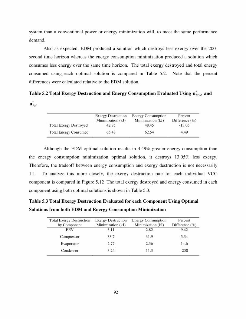
92

system than a conventional power or energy minimization will, to meet the same performance

demand.

Also as expected, EDM produced a solution which destroys less exergy over the 200-

second time horizon whereas the energy consumption minimization produced a solution which

consumes less energy over the same time horizon. The total exergy destroyed and total energy

consumed using each optimal solution is compared in Table 5.2. Note that the percent

differences were calculated relative to the EDM solution.

Table 5.2 Total Exergy Destruction and Energy Consumption Evaluated Using *uEDM

and

*uPM

Exergy Destruction

Minimization (kJ)

Energy Consumption

Minimization (kJ)

Percent

Difference (%)

Total Exergy Destroyed 42.85 48.45 -13.05

Total Energy Consumed 65.48 62.54 4.49

Although the EDM optimal solution results in 4.49% greater energy consumption than

the energy consumption minimization optimal solution, it destroys 13.05% less exergy.

Therefore, the tradeoff between energy consumption and exergy destruction is not necessarily

1:1. To analyze this more closely, the exergy destruction rate for each individual VCC

component is compared in Figure 5.12 The total exergy destroyed and energy consumed in each

component using both optimal solutions is shown in Table 5.3.

Table 5.3 Total Exergy Destruction Evaluated for each Component Using Optimal

Solutions from both EDM and Energy Consumption Minimization

Total Exergy Destruction

by Component

Exergy Destruction

Minimization (kJ)

Energy Consumption

Minimization (kJ)

Percent

Difference (%)

EEV 3.11 2.82 9.42

Compressor 33.7 31.9 5.34

Evaporator 2.77 2.36 14.6

Condenser 3.24 11.3 -250

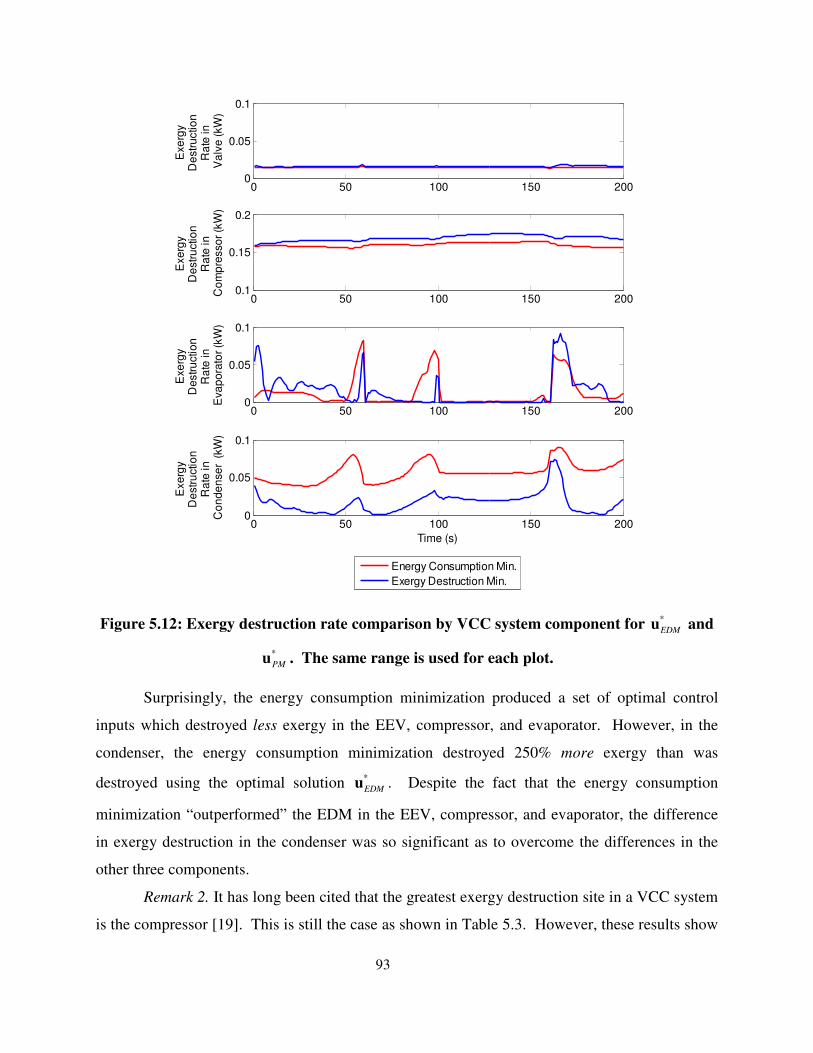
93

Figure 5.12: Exergy destruction rate comparison by VCC system component for *uEDM

and

*uPM

. The same range is used for each plot.

Surprisingly, the energy consumption minimization produced a set of optimal control

inputs which destroyed less exergy in the EEV, compressor, and evaporator. However, in the

condenser, the energy consumption minimization destroyed 250% more exergy than was

destroyed using the optimal solution *

EDMu . Despite the fact that the energy consumption

minimization “outperformed” the EDM in the EEV, compressor, and evaporator, the difference

in exergy destruction in the condenser was so significant as to overcome the differences in the

other three components.

Remark 2. It has long been cited that the greatest exergy destruction site in a VCC system

is the compressor [19]. This is still the case as shown in Table 5.3. However, these results show

0 50 100 150 2000

0.05

0.1

Exe

rgy

De

str

uctio

n

Ra

te in

V

alv

e (

kW

)



0 50 100 150 2000.1

0.15

0.2

Exerg

y

De

str

uctio

n

Ra

te in

Co

mp

resso

r (k

W)

0 50 100 150 2000

0.05

0.1

Exe

rgy

Destru

ction

R

ate

in

E

va

pora

tor (k

W)

0 50 100 150 2000

0.05

0.1

Time (s)

Exerg

y

De

str

uctio

n

Ra

te in

Co

nde

nse

r (

kW

)

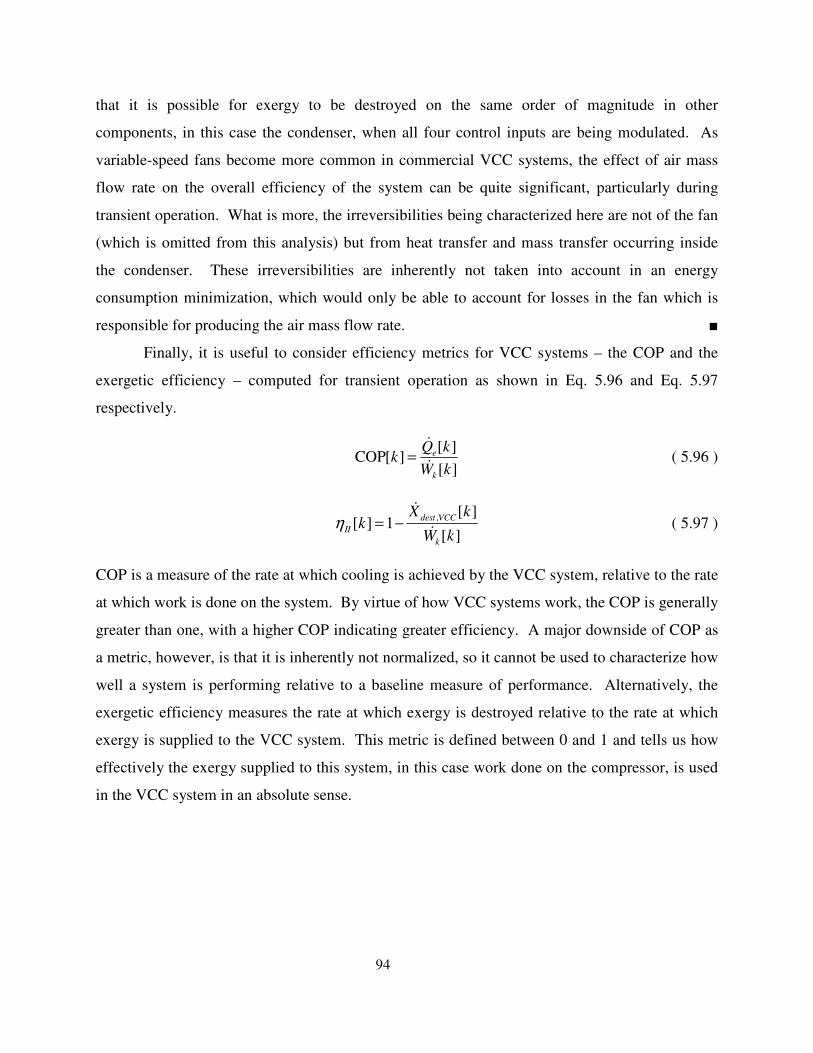
94

that it is possible for exergy to be destroyed on the same order of magnitude in other

components, in this case the condenser, when all four control inputs are being modulated. As

variable-speed fans become more common in commercial VCC systems, the effect of air mass

flow rate on the overall efficiency of the system can be quite significant, particularly during

transient operation. What is more, the irreversibilities being characterized here are not of the fan

(which is omitted from this analysis) but from heat transfer and mass transfer occurring inside

the condenser. These irreversibilities are inherently not taken into account in an energy

consumption minimization, which would only be able to account for losses in the fan which is

responsible for producing the air mass flow rate. ■

Finally, it is useful to consider efficiency metrics for VCC systems – the COP and the

exergetic efficiency – computed for transient operation as shown in Eq. 5.96 and Eq. 5.97

respectively.

[ ]

[ ]COP[ ] e

k

Qk

W

k

k=ɺ

ɺ ( 5.96 )

, [ ]

[ ] 1[ ]

dest VCC

II

k

X kk

W kη = −

ɺ

ɺ ( 5.97 )

COP is a measure of the rate at which cooling is achieved by the VCC system, relative to the rate

at which work is done on the system. By virtue of how VCC systems work, the COP is generally

greater than one, with a higher COP indicating greater efficiency. A major downside of COP as

a metric, however, is that it is inherently not normalized, so it cannot be used to characterize how

well a system is performing relative to a baseline measure of performance. Alternatively, the

exergetic efficiency measures the rate at which exergy is destroyed relative to the rate at which

exergy is supplied to the VCC system. This metric is defined between 0 and 1 and tells us how

effectively the exergy supplied to this system, in this case work done on the compressor, is used

in the VCC system in an absolute sense.

95

Figure 5.13: Instantaneous COP and exergetic efficiency resulting from operating the

system with *uEDM

and *uPM

.

Figure 5.13 shows that the energy consumption minimization operates the system at a

higher COP but with a lower exergetic efficiency. On average, the COP achieved by minimizing

exergy destruction was 4.68% lower than that achieved by minimizing energy consumption. On

the other hand, on average, the exergetic efficiency achieved by minimizing exergy destruction

was 36.6% greater than that achieved by minimizing energy consumption. These results indicate

that although the EDM optimal solution would operate the system in such a way as to consume

more energy, that energy is being used by the system more “effectively”. To be more precise,

this means operating the system with fewer irreversibilities, such as friction in refrigerant flow

and losses in heat transfer across finite temperature differences. Operating the system in this

way can have implications on the wear of the physical components themselves, a longer term

objective for the operation of thermal systems which was not explicitly accounted for in either

objective function considered in this case study.

5.4.3 Summary

To summarize, the results in this section showed that during transient operation of a VCC

system, there exists a distinct tradeoff in system operation based on minimization of exergy

destruction versus minimization of energy consumption. Major conclusions are reiterated below.

0 50 100 150 2002.2

2.4

2.6

2.8

3

3.2

CO

P



0 50 100 150 2000

0.1

0.2

0.3

0.4

Time (s)

Exe

rge

tic E

ffic

ien

cy

96

� Exergy destruction minimization and energy consumption minimization are not

equivalent when the dynamic exergy destruction rate for a VCC system is

considered.

� The dynamic EDM objective function specifically accounted for irreversibilities

in each component of the VCC whereas the energy consumption minimization did

not.

� The distribution of exergy destruction across the components of the VCC system

changes as a function of the control inputs, demonstrating not only the importance

of considering the dynamic exergy destruction rate but also of optimal control of

VCC systems with full actuation.

� Minimizing total exergy destruction leads to operation with a higher exergetic

efficiency which may result in less component wear over time.

97

Chapter 6

Conclusion

6.1 Summary of Research Contributions

Integrated energy systems (IESs) are complex systems which operate across multiple

energy domains and offer a reliable and efficient way to generate both electrical power and

thermal energy to meet multiple end requirements. In order to operate these systems effectively,

setpoint optimization and/or optimal control is needed. In this thesis, an optimization and control

framework for the operation of IESs was developed with a specific emphasis on providing a

systematic method for obtaining a physics-based, generalizable, and modular objective function.

We have proposed the use of exergy destruction as the metric for obtaining such a

versatile objective function. Exergy destruction minimization (EDM) is a tool which has

primarily been used for design optimization but not for real-time optimization and control of

thermodynamic and other energy systems. Nevertheless, it is well suited for IESs because it can

fully characterize irreversibilities across multiple energy domains. Moreover, the exergy

destruction rate for a complex system can be derived by analyzing subsystems and/or

components individually and then summing these rates for the overall system.

The generalizability and modularity of the framework was demonstrated through its

application to a combined cooling, heating, and power (CCHP) system. The CCHP system was

easily divided into 4 subsystems which were analyzed individually, thereby greatly simplifying

the derivation of the complete objective function. An additional layer of flexibility was

introduced as the “interchangeability” between power minimization and exergy destruction rate

minimization for those subsystems in which the reversible power is constant with respect to the

decision variables. Interchangeability allows the user to only derive the exergy destruction rate

98

for those systems in which the equivalence does not hold and construct an objective function

which would result in the same solution as minimizing the rate of exergy destruction in every

subsystem.

Exergy analyses have long been used to better understand the behavior of a variety of

thermodynamic systems, primarily from a static design and operation point of view. However,

as the complexity of integrated energy systems grows, for example as a result of intermittent grid

power from renewable energy technologies such as wind and solar, an understanding of transient

behavior is needed. As a case study, a detailed derivation of the dynamic exergy destruction rate

in a standard VCC system was derived for the refrigerant-side dynamics assuming a lumped

parameter moving boundary model framework for the heat exchanger dynamics. The dynamic

rate of exergy destruction was then used in formulating an EDM optimal control problem for a

VCC system wherein the decision variables were the control inputs to the system. Moreover, the

VCC system was assumed to be fully actuated with an electronic expansion valve (EEV), and

variable-speed compressor, evaporator fan, and condenser fan. The results highlighted how

time-varying control decisions can affect the distribution of irreversibilities throughout the

overall system, particularly in the heat exchangers which are typically considered to have fewer

irreversibilities compared to the compressor and EEV.

The relationship between exergy destruction rate, power consumption, and reversible

power was utilized throughout this work to specifically characterize when tradeoffs exists

between the minimization of energy consumption versus exergy destruction. During both

steady-state operation of the CCHP system and transient operation of the VCC system, it was

shown that minimizing exergy destruction increases exergetic efficiency at some expense of

energy consumption, but that the decrease in exergy destruction can possibly outweigh the

increases in energy consumption.

As electrification of individual and integrated energy systems continues to increase,

model-based optimization and control techniques offer many tools for improving the efficiency

of such systems during many different modes of operation. This thesis showed that an exergy

destruction minimization has the potential to uncover a different set of solutions than those

produced by an energy or power minimization, and should therefore be considered as a valuable

tool for operational optimization of IESs. Moving forward, increased complexity and a greater

99

diversity of systems can be analyzed to ensure that this potential does indeed scale across a wide

class of IESs. Specific areas of future investigation are detailed in the next section.

6.2 Future Work

The generalizability and modularity of the approach are key features which are needed

for widespread applicability of this framework to IESs. Further investigation should include

consideration of irreversibilities in non-thermodynamic energy systems, such as wind turbines,

and in storage devices, such as chemical batteries or chilled water storage tanks. These

subsystems are becoming integral parts of IESs. Energy storage devices particularly lend

themselves to the EDM approach because they neither produce nor consume energy but instead

are used for the transfer of energy from one medium to another (and also often one form of

energy to another). The storage and discharge processes are inherently irreversible, and these

losses affect the overall efficiency of a given system.

Exergy destruction minimization has not previously been combined with optimal control

algorithms for online control of energy systems. Based on the results of this work, further

complexity can be addressed. The dynamic exergy destruction rate derived for the standard

VCC system currently does not account for irreversibilities on the secondary fluid side of the

heat exchangers, nor the two components which act solely on the secondary fluid – the heat

exchanger fans. An augmentation of the dynamic exergy rate to include these features will offer

further insight into the distribution of irreversibilities in the system during transient operation,

particularly during high frequency actuation of the system.

It is also important to validate the ideas proposed in this work on physical hardware to

gain a deeper understanding of the benefits of EDM for operational optimization of energy

systems. To make the dynamic EDM metric more viable for experimental implementation,

additional investigation should consider alternative nonlinear search algorithms which may

increase the speed of solving the optimal control problem. Moreover, in the specific case of

VCC systems, alternative formulations of the control architecture, such as a time-scale separation

of the fast and slow dynamics, can be considered.

100

List of References

[1] D. Wu and R. Wang, "Combined cooling, heating and power: A review," Progress in Energy and

Combustion Science, vol. 32, no. 5-6, pp. 459-495, 2006.

[2] "Combined heat and power partnership," U.S. Environmental Protection Agency, 12 September

2012. [Online]. Available: http://epa.gov/chp/index.html.

[3] P. LeMar, "Integrated Energy Systems (IES) for Buildings: A Market Assessment," Resource

Dynamics Corporation, 2002.

[4] "White House Announces Executive Order on Industrial Energy Efficiency, including Combined

Heat and Power," Federal Energy Management Program, 30 August 2012. [Online]. Available:

http://www1.eere.energy.gov/femp/news/news_detail.html?news_id=18599.

[5] M. Hosseini, I. Dincer and M. A. Rosen, "Hybrid solar-fuel cell combined heat and power systems

for residential applications: Energy and exergy analyses," Journal of Power Sources, vol. 221, pp.

372-380, 2013.

[6] X. P. Chen, Y. D. Wang, H. D. Yu, D. W. Wu, Y. Li and A. P. Roskilly, "A domestic CHP system

with hybrid electrical energy storage," Energy and Buildings, 2012.

[7] "Combined heat and power technology fills an important energy niche," U.S. Energy Information

Administration, 4 October 2012. [Online]. Available:

http://www.eia.gov/todayinenergy/detail.cfm?id=8250#.

[8] O. A. Shaneb, P. C. Taylor and G. Coates, "Optimal online operation of residential mu systems

using linear programming," Energy and Buildings, vol. 44, pp. 17-25, 2012.

[9] H. Cho, R. Luck and L. M. Chamra, "Supervisory Feed-Forward Control for Real-Time Topping

Cycle CHP Operation," Journal of Energy Resources Technology, 2010.

[10] V. Tsourapas, A. Stefanopoulou and J. Sun, "Dynamics, optimization and control of a fuel cell

based combined heat power (chp) system for shipboard applications," in Proceedings of the 2005

101

American Control Conference, 2005.

[11] A. Y. Petrov, A. Zaltash, S. D. Labinov, D. T. Rizy and R. L. Linkous, "Dynamic performance of a

30-kW microturbine-based CHP system," ASHRAE Transactions, vol. 111, no. 1, 2005.

[12] X. Q. Kong, R. Z. Wang and X. H. Huang, "Energy optimization model for a CCHP system with

available gas turbines," Applied Thermal Engineering, vol. 25, no. 2, pp. 377-391, 2005.

[13] T. A. Reddy and I. Maor, "Cost penalties of near optimal scheduling control of BCHP systems: part

II - modeling, optimization, and analysis results," ASHRAE Transactions, vol. 115, no. 1, pp. 287-

307, 2009.

[14] H. Cho, R. Luck, S. D. Eksioglu and L. M. Chamra, "Cost-optimized real-time operation of CHP

systems," Energy and Buildings, vol. 41, no. 4, pp. 445-451, 2009.

[15] E. Thorin, H. Brand and C. Weber, "Long-term optimization of cogeneration systems in a

competitive market environment," Applied Energy, vol. 81, no. 2, pp. 152-169, 2005.

[16] M. J. Moran and H. N. Shapiro, Fundamentals of Engineering Thermodynamics, John Wiley &

Sons, Inc., 2004.

[17] A. Bejan, Entropy Generation Minimization, Boca Raton: CRC Press LLC, 1996q.

[18] Y. A. Cengel and M. A. Boles, Thermodynamics: An Engineering Approach, 6th ed., Boston: The

McGraw-Hill Companies, Inc., 2008.

[19] T. J. Kotas, The Exergy Method of Thermal Plant Analysis, London: Butterworths, 1985.

[20] J. U. Ahamed, R. Saidur and H. H. Masjuki, "A review on exergy analysis of vapor compression

refrigeration system," Renewable and Sustainable Energy Reviews, vol. 15, no. 3, pp. 1593-1600,

2011.

[21] H. Mahabadipour and H. Ghaebi, "Development and comparison of two expander cycles used in

refrigeration system of olefin plant based on exergy analysis," Applied Thermal Engineering, vol.

50, no. 1, pp. 771-780, 2012.

[22] A. Cihan, O. Hachafzoglu and K. Kahveci, "Energy-exergy analysis and modernization suggestions

for a combined-cycle power plant," International Journal of Energy Research, vol. 30, no. 2, pp.

115-126, 2006.

[23] G. Tsatsaronis, "Thermoeconomic Analysis and Optimization of Energy Systems," Progress in

Energy and Combustion Science, vol. 19, no. 3, pp. 227-257, 1993.

[24] G. Tsatsaronis and M. J. Moran, "Exergy-Aided Cost Minimization," Energy Conversion and

Management, vol. 38, no. 15-17, pp. 1535-1542, 1997.

102

[25] A. Abusoglu and M. Kanoglu, "Exergoeconomic analysis and optimization of combined heat and

power production: A review," Renewable and Sustainable Energy Reviews, vol. 13, pp. 2295-2308,

2009.

[26] A. Lazzaretto and G. Tsatsaronis, "SPECO: A systematic and general methodology for calculating

efficiencies and costs in thermal systems," Energy, vol. 31, no. 8-9, pp. 1257-1289, 2006.

[27] A. Bejan, "Fundamentals of exergy analysis, entropy generation minimization, and the generation of

flow architecture," International Journal of Energy Research, vol. 26, pp. 545-565, 2002.

[28] R. J. Krane, "A Second Law analysis of the optimum design and operation of thermal energy storage

systems," International Journal of Heat and Mass Transfer, vol. 30, no. 1, pp. 43-57, 1987.

[29] W. G. le Roux, T. Bello-Ochende and J. P. Meyer, "Thermodynamic optimisation of the integrated

design of a small-scale solar thermal Brayton cycle," International Journal of Energy Research, vol.

36, pp. 1088-1104, 2012.

[30] P. K. Nag and S. De, "Design and Operation of a Heat Recovery Steam Generator with Minimum

Irreversibility," Applied Thermal Engineering, vol. 17, no. 4, pp. 385-391, 1997.

[31] J. Vargas and A. Bejan, "Thermodynamic optimization of finned crossflow heat exchangers for

aircraft environmental control systems," International Journal of Heat and Fluid Flow, vol. 22, pp.

657-665, 2001.

[32] B. David, J. Ramousse and L. Luo, "Optimization of thermoelectric heat pumps by operating

condition management and heat exchanger design," Energy Conversion and Management, vol. 60,

pp. 125-133, 2012.

[33] N. Jain and A. G. Alleyne, "A framework for the optimization of integrated energy systems,"

Applied Thermal Engineering, vol. 48, pp. 495-505, 2012.

[34] V. Chandan, A.-T. Do, B. Jin, F. Jabbari, J. Brouwer, I. Akrotirianakis, A. Chakraborty and A.

Alleyne, "Modeling and Optimization of a Combined Cooling, Heating and Power Plant System," in

Proceedings of ACC 2012, the 31st American Control Conference, Montreal, 2012.

[35] V. Chandan and A. Torzhkov, "Gray-Box Model Formulation of a Cogenerating Microgrid, Part 1:

Physical Formulation," 2011. [Online]. Available:

http://mechse.illinois.edu/media/uploads/web_sites/104/files/cchp_modeling_chandan_vikas_2011.2

0121117.50a84437378641.65743102.pdf. [Accessed September 2012].

[36] A. H. Harvey, A. P. Peskin and S. A. Klein, NIST Standard Reference Database 10, Boulder:

National Institute of Standards and Technology, 1997.

[37] M. Pidwirny, "Chapter 7: Introduction to the Atmosphere," May 2009. [Online]. Available:

103

http://www.physicalgeography.net/fundamentals/7l.html. [Accessed September 2012].

[38] X. Li and J. M. Ogden, "Understanding the design and economics of distributed tri-generation

systems," Journal of Power Sources, no. 197, pp. 186-195, 2012.

[39] L. Ni, S. K. Lau, H. Li, T. Zhang, J. S. Stansbury, J. Shi and J. Neal, "Feasibility study of a localized

residential grey water energy-recovery system," Applied Thermal Engineering, no. 39, pp. 53-62,

2012.

[40] Toolbox, MATLAB Optimization, The Mathworks Inc., Natick, MA, 2002.

[41] W. Stoecker and J. Jones, Refrigeration and Air-Conditioning, New York: McGraw-Hill Book

Company, 1983.

[42] T. Q. Qureshi and S. A. Tassou, "Variable-speed capacity control in refrigeration systems," Applied

Thermal Engineering, vol. 16, no. 2, pp. 103-113, 1996.

[43] Braven, K. D, Penoncello, S., Herold, K., et. al., "Improving heat pumps and air conditioning,"

Mechanical Engineering, vol. 115, no. 9, 1993.

[44] X. D. He, S. Liu, H. H. Asada and H. Itoh, "Multivariable Control of Vapor Compression Systems,"

HVAC&R Research, vol. 4, no. 3, pp. 205-230, 1998.

[45] L. S. Larsen, C. Thybo, J. Stoustrup and H. Rasmussen, "Control methods utilizing energy

optimizing schemes in refrigeration systems," in European Control Conference, 2003.

[46] L. F. S. Larsen and C. Thybo, "Potential energy savings in refrigeration systems using optimal

setpoints," in Conference on Control Applications, 2002.

[47] J. B. Jensen and S. Skogestad, "Optimal operation of simple refrigeration cycles; Part I: Degrees of

freedom and optimality of sub-cooling," Computers and Chemical Engineering, vol. 31, no. 5-6, pp.

712-721, 2007.

[48] M. S. Elliott and B. P. Rasmussen, "A Model-Based Predictive Supervisory Controller for Multi-

Evaporator HVAC Systems," in Proceedings of the American Control Conference, 2009.

[49] R. Shah, B. P. Rasmussen and A. G. Alleyne, "Application of a Multivariable Adaptive Control

Strategy to Automotive Air Conditioning Systems," International Journal of Adaptive Control and

Signal Processing, vol. 18, no. 2, pp. 199-221, 2004.

[50] L. F. S. Larsen, C. Thybo, J. Stoustrup and H. Rasmussen, "A Method for Online Steady State

Energy Minimization with Application to Refrigeration Systems," in Proceedings of the 43rd IEEE

Conference on Decision and Control, 2004.

[51] N. Jain, B. Li, M. Keir, B. Hencey and A. Alleyne, "Decentralized Feedback Structures of a Vapor

104

Compression Cycle System," IEEE Transactions on Control Systems Technology, vol. 18, no. 1, pp.

185-193, 2010.

[52] F. P. Incropera and D. P. DeWitt, Fundamentals of Heat and Mass Transfer, New York: John Wiley

and Sons Inc., 1985.

[53] B. Eldredge, Improving the Accuracy and Scope of Control-Oriented Vapor Compression Cycle

System Models, Master's thesis, University of Illinois at Urbana-Champaign, 2006.

[54] ASHRAE Handbook: Fundamentals, American Society of Heating, Refrigeration, and Air-

Conditioning Engineers, Inc., 2009.

[55] L. Ljung, System Identification Toolbox for Use with MATLAB, 2007.

[56] K. Ogata, Modern Control Engineering, 4th ed., Prentice Hall, 2002.

[57] R. Otten, Superheat Control for Air Conditioning and Refrigeration Systems: Simulation and

Experiments, Master's Thesis: University of Illinois at Urbana-Champaign, 2010.

[58] G. Anand, M. Mahajan, N. Jain, B. Maniam and T. M. Tumas, "e-Thermal: Automobile Air

Conditioning Module," in Society of Automotive Engineers 2004 World Congress, Detroit, 2004.

[59] H. Tummescheit and J. Eborn, "Design of a Thermo-Hydraulic Model Library in Modelica," in 12th

European Simulation Multiconference, San Diego.

[60] B. A. Cullimore and T. J. Hendricks, "Design and Transient Simulation of Vehicle Air Conditioning

Systems," in Society of Automotive Engineers 2004 World Congress, Detroit, 2004.

[61] S. Bendapudi and J. E. Braun, "A Review of Literature on Dynamic Models of Vapor Compression

Equipment," ASHRAE Report #4036-5, May 2002.

[62] T. L. McKinley and A. G. Alleyne, "An advanced nonlinear switched heat exchanger model for

vapor compression cycles using the moving-boundary method," International Journal of

Refrigeration, vol. 31, no. 7, pp. 1253-1264, 2008.

[63] B. Li and A. G. Alleyne, "A dynamic model of a vapor compression cycle with shut-down and start-

up operations," International Journal of Refrigeration, vol. 33, no. 3, pp. 538-552, 2010.

[64] J. H. Doty, J. A. Camberos and K. L. Yerkes, "Approximate Approach for Direct Calculation of

Unsteady Entropy Generation Rate for Engineering Applications," in Proceedings of the 50th AIAA

Aersopace Sciences Meeting, Nashville, 2012.

[65] B. P. Rasmussen, Control-Oriented Modeling of Transcritical Vapor Compression Systems, Urbana,

IL: University of Illinois at Urbana-Champaign, M.S. Thesis, 2000.

[66] M. Kania, J. Koeln, A. Alleyne, K. McCarthy , N. Wu and S. Patnaik, "A Dynamic Modeling

105

Toolbox for Air Vehicle Vapor Cycle Systems," in SAE Power Systems International, Phoenix, AZ,

2012.

[67] B. P. Rasmussen, Dynamic Modeling and Advanced Control of Air Conditioning and Refrigeration

Systems, Urbana, IL: University of Illinois at Urbana-Champaign, Ph.D. Thesis, 2005.

[68] J. Nocedal and S. J. Wright, Numerical Optimization, New York: Springer Science+Business

Media, LLC., 2006.

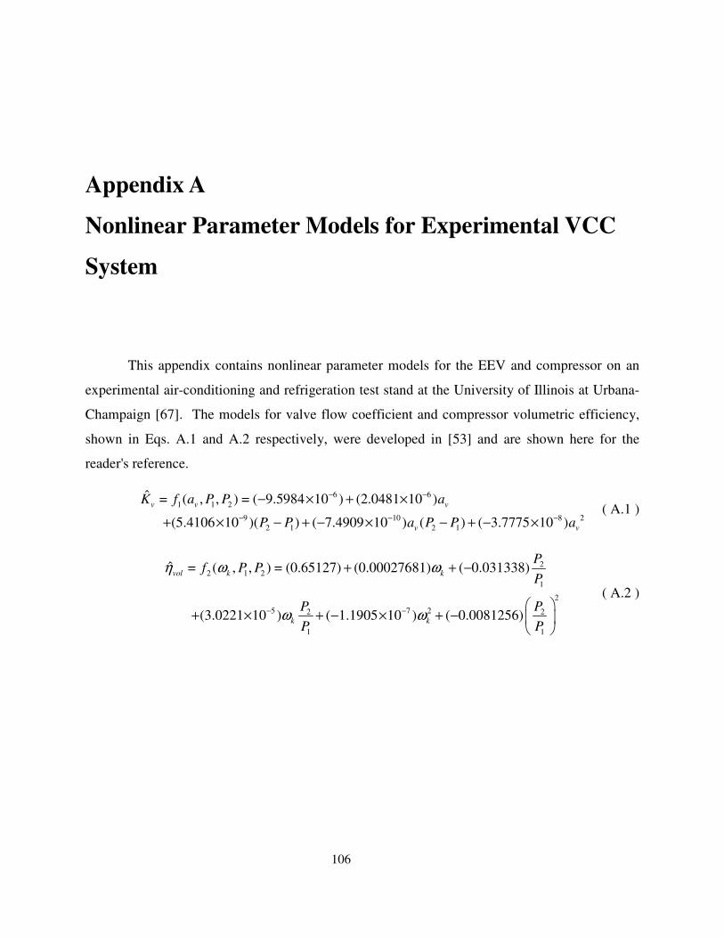
106

Appendix A

Nonlinear Parameter Models for Experimental VCC

System

This appendix contains nonlinear parameter models for the EEV and compressor on an

experimental air-conditioning and refrigeration test stand at the University of Illinois at Urbana-

Champaign [67]. The models for valve flow coefficient and compressor volumetric efficiency,

shown in Eqs. A.1 and A.2 respectively, were developed in [53] and are shown here for the

reader's reference.

6 6

1 1 2

9 10 8 2

2 1 2 1

ˆ = ( , , ) = ( 9.5984 10 ) (2.0481 10 )

(5.4106 10 )( ) ( 7.4909 10 ) ( ) ( 3.7775 10 )

v v

v

v

v

K f a P P a

P P a P P a

− −

− − −

− × + ×

+ × − + − × − + − × ( A.1 )

22 1 2

1

2

5 7 22 2

1 1

ˆ = ( , , ) = (0.65127) (0.00027681) ( 0.031338)

(3.0221 10 ) ( 1.1905 10 ) ( 0.0081256)

vol k

k k

k

Pf P P

P

P P

P P

η ω

ω ω

ω

− −

+ + −

+ × + − × + −

( A.2 )

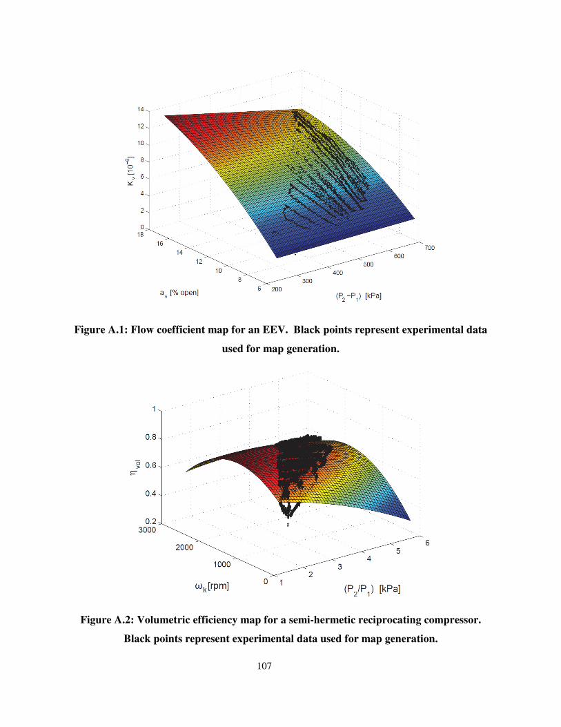
107

Figure A.1: Flow coefficient map for an EEV. Black points represent experimental data

used for map generation.

Figure A.2: Volumetric efficiency map for a semi-hermetic reciprocating compressor.

Black points represent experimental data used for map generation.

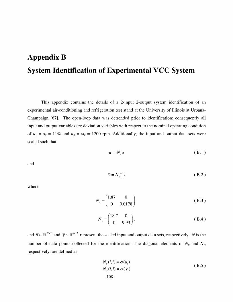
108

Appendix B

System Identification of Experimental VCC System

This appendix contains the details of a 2-input 2-output system identification of an

experimental air-conditioning and refrigeration test stand at the University of Illinois at Urbana-

Champaign [67]. The open-loop data was detrended prior to identification; consequently all

input and output variables are deviation variables with respect to the nominal operating condition

of u1 = av = 11% and u2 = ωk = 1200 rpm. Additionally, the input and output data sets were

scaled such that

= uu N u ( B.1 )

and

1=y

y N y− ( B.2 )

where

1.87 0

= ,0 0.0178

uN

( B.3 )

18.7 0

= ,0 9.93

yN

( B.4 )

and 2Nu

×∈ℝ and 2N

y×∈ℝ represent the scaled input and output data sets, respectively. N is the

number of data points collected for the identification. The diagonal elements of Nu and Ny,

respectively, are defined as

( , ) = ( )

( , ) = ( )

u i

y i

N i i u

N i i y

σ

σ ( B.5 )

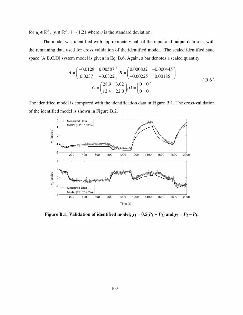
109

for N

iu ∈ℝ , N

iy ∈ℝ , i ={1,2} where σ is the standard deviation.

The model was identified with approximately half of the input and output data sets, with

the remaining data used for cross validation of the identified model. The scaled identified state

space [A,B,C,D] system model is given in Eq. B.6. Again, a bar denotes a scaled quantity.

0.0128 0.00587 0.000832 0.000445= , =

0.0237 0.0322 0.00225 0.00185

28.9 3.02 0 0= , =

12.4 22.0 0 0

A B

C D

− −

− −

( B.6 )

The identified model is compared with the identification data in Figure B.1. The cross-validation

of the identified model is shown in Figure B.2.

Figure B.1: Validation of identified model; y1 = 0.5(P1 + P2) and y2 = P2 – P1.

200 400 600 800 1000 1200 1400 1600 1800 2000-2

-1

0

1

2

y1 (

sca

led

)

200 400 600 800 1000 1200 1400 1600 1800 2000-4

-2

0

2

4

Time (s)

y2 (

sca

led

)

Measured Data

Model (Fit: 67.58%)

Measured Data

Model (Fit: 57.43%)

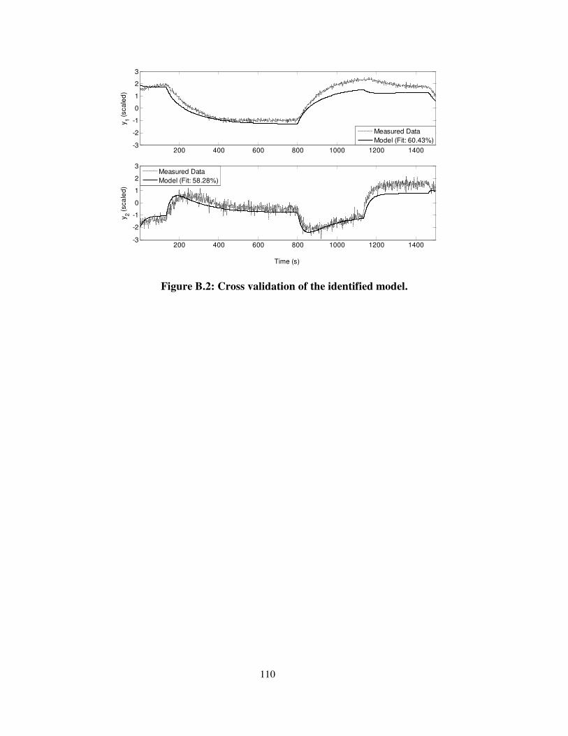
110

Figure B.2: Cross validation of the identified model.

200 400 600 800 1000 1200 1400-3

-2

-1

0

1

2

3

y 1 (

sca

led

)

200 400 600 800 1000 1200 1400-3

-2

-1

0

1

2

3

Time (s)

y 2 (

sca

led

)

Measured Data

Model (Fit: 60.43%)

Measured Data

Model (Fit: 58.28%)

111

Appendix C

VCC System Model Linearization

This appendix describes the linearization procedure used to obtain a first-principles

linearized model of a standard VCC system in the lumped parameter moving boundary modeling

framework.

C.1 Individual Component Linearization

C.1.1 Linearization of Heat Exchanger Models

The linearization procedure for the lumped parameter moving boundary heat exchanger

models is described in detail in [67]. The procedure is summarized here for the benefit of the

reader. The governing equations for a given heat exchanger model in the lumped parameter

moving boundary framework can be written in the form

( ) ( ),·, fZ =x u x x uɺ ( C.1 )

where Z can be assumed to be invertible. Then the state derivative vector can be expressed as

( ) ( )

( )

1

.

, ,

,

· fZ

g

−=

=

x x u x u

x u

ɺ ( C.2 )

Linearizing the system about some operating condition (x0,u0) where = − 0δx x x and = − 0δu u u

yields

, ,

g gδ δ δ

∂ ∂ ∂

+∂

=0 0 0 0x u x u

x x ux u

ɺ ( C.3 )

112

which can be rewritten as

( ) ( ), ,

.g g

= − + ∂ ∂ ∂ ∂

−0 0 0 0

0 0

x u x u

x x x u ux u

ɺ ( C.4 )

Expanding the first term in Eq. C.4 results in

( ) ( ), ,

11 2

,, , ,

· · .g f Z

Z Z f

−− − ∂ ∂ ∂

= − ∂ ∂ ∂ 0 0 0 0 0 0

0 0 0 0 0 0

x u x u x ux u x u x ux x x

( C.5 )

If the linearization point is chosen to be an equilibrium point of the system, then

( ),

0,f f= =0 0

0 0x ux u ( C.6 )

thereby simplifying Eq. C.5 to

( )1

,, , .

·g f

Z−∂ ∂

=∂ ∂0 0

0 0 0 0

x ux u x ux x

( C.7 )

Similarly, for the second term in Eq. C.4, choosing (x0,u0) to be an equilibrium point of the

system results in

( )1

,, , .

·g f

Z−∂ ∂

=∂ ∂0 0

0 0 0 0

x ux u x uu u

( C.8 )

Substituting Eq. C.7 and Eq. C.8 into Eq. C.4 yields

( ) ( ) ( ) ( ), ,

, ,

1 1

· ·f f

Z Z− −

= − + −

∂ ∂

∂ ∂0 0 0 0

0 0 0 0

0 0x u x ux u x u

x x x u ux u

ɺ ( C.9 )

which is in the familiar state space form of

δ δ= +x A x B uɺ ( C.10 )

where

( )1

,,

1· x

fZ Z F

−−∂

=∂

=0 0

0 0

x ux u

Ax

( C.11 )

and

113

( )1

1

,,

· .u

fZ Z F

−−∂

=∂

=0 0

0 0

x ux u

Bu

( C.12 )

In the next section, this procedure is demonstrated for the evaporator model with two

refrigerant fluid regions. Since the linearization procedure is analogous for the condenser model

with three refrigerant fluid regions, details of that linearization will not be provided in this

appendix. The governing equations for the condenser model are provided in [66].

C.1.1.1 Evaporator Model with Two Refrigerant Fluid Regions

The mass and energy conservation equations for the two-phase refrigerant fluid region in

the evaporator are given in Eq. C.13 and Eq. C.14, respectively.

,1 1 1 1 1 12

1 1 1 1

e ine e e e e e e e

e e e e e e e e

md dP d m

dt P dt dt V V

ζ ζ ρ ζ ρ γ

ρ ρ γ ρ ρ

∂ ∂+ + + =

∂ ∂

ɺɺ ( C.13 )

, 1 1 , , 11 112

1 1 1 1 1

( )1 e g e e e in e in ee e e e

e

e e e e e e e e e

h h Q m h hh dP h dm

P dt dt V V

γ

ρ γ ρ ζ ρ ζ

− + − ∂ ∂− + + =

∂ ∂

ɺ ɺɺ ( C.14 )

The mass and energy conservation equations for the superheated refrigerant fluid region in the

evaporator are given in Eq. C.15 and Eq. C.16, respectively.

,1 2 2 2 2 2 12

2 2 2 2 2

e oute e e e e e e e

e e e e e e e e

md dP dh m

dt P dt h dt V V

ζ ζ ρ ζ ρ

ρ ρ ρ ρ

∂ ∂− − + =

∂ ∂

ɺɺ ( C.15 )

, 2 2 , 2 ,212

2 2 2 2 2

( )1 e g e e e out e e ge ee

e e e e e e e

h h Q m h hdP dhm

dt dt V Vρ ρ ζ ρ ζ

− − −− + − =

ɺ ɺɺ ( C.16 )

The governing equation for mean-void fraction is given in Eq. C.17.

( ),

, ,

tot e e ee e e tot

e

dP dK

P dt dtγ

γ γγ γ

∂− = −

∂ ( C.17 )

The governing equations for the tube wall in the two-phase and superheated regions respectively

are

( ), 1 11 , 1 , 1 1, 1,( ) ( )

w e eew e ew wt e w e e r e a

dT dmc mc T T Q Q

dt dt

ζζ − − = − −ɺ ɺ ( C.18 )

and

114

( ), 2 12 , 2 , 1 2, 2 ,( ( .) )

w e eew e ew w e wt e e r e a

dT dmc mc T T Q Q

dt dt

ζζ − − = − −ɺ ɺ ( C.19 )

These 6 nonlinear equations can written in the matrix form e e eZ f=xɺ where

[ ]

( ) ( ) ( )

( ) ( )

1 2 2 1

1 2 1 2 2 1

2

2 2, 2 2 2 , 2 2 2 , 2

2

1

1 , 1 1 1 , 1

1

0

1

1

0 0

0

0

e e e e

e e e e e e e e e e

e e e e

e ee g e e e e e e g e e e e e g e

e e

e e

e e e g e e e e e g e

e e

e

V V V VP P h

h h V V h h V h hP h

hV h h V h h

PZ

ρ ρ ρ ρρ ρ ζ ζ ζ ζ

γ

ρ ρρ ζ ζ ρ

ρρ ζ ρ

ρ

∂ ∂ ∂ ∂− +

∂ ∂ ∂ ∂

∂ ∂− − + − − −

∂ ∂

∂ ∂ − − − −

− ∂

=

( )

( )

( )

1 1 1

1 1 , 1

, 1 , 1 1

, 2 , 1 2

,

0

( ) ( ) 0

( ) 0 ( )

0

0 0

,

0 0 0

0 0 0

0 0 0 1

e e

e e e e g e

e e e

ew wt e w e ew e

ew w e wt e ew e

e tot

e

hV h h

P

mc T T mc

mc T T mc

P

ρζ ρ

γ γ

ζ

ζ

γ

∂ ∂− −

∂ ∂ ∂

− −

− −

∂

∂−

( C.20 )

1

2

, 1

, 2

,

e

e

e

e

w e

w e

e

P

h

T

T

ζ

γ

=x

ɺ

ɺ

ɺɺ

ɺ

ɺ

ɺ

( C.21 )

and

( )

( )

( )

, ,

2, , , 2

1, , ,

1, 1,

2, 2

,

,

, ,

2

.

e in e out

e r e out e g e

e r e in e in

e

e r e a

e r e a

e e e tot

e g

m m

Q m h h

Q m h hf

Q Q

Q Q

K γ γ γ

+ − + − = − − − − −

−ɺ ɺ

ɺ ɺ

ɺ

ɺ

ɺ

ɺ

ɺ ɺ

( C.22 )

Detailed expressions for the heat transfer rates 1,e rQɺ , 2,e rQɺ , 1,e aQɺ , and 2,e aQɺ , are given in Eq. C.23.

( )

( )

( )

( )

1, 1 1 , 1 , 1

2, 2 2 , 2 , 2

1, 1 , 1, ,

2, 2 , 2

,

, , ,

e r e e e w e r e

e r e e e w e r e

e a e p a e ao e ai

e a e p a e ao e ai

a e

a e

Q A T

Q A T

Q m c T

Q m

T

T

T

c TT

ζ α

ζ α

ζ

ζ

=

=

=

=

−

−

−

−

ɺ ɺ

ɺ ɺ

ɺ

ɺ ( C.23 )

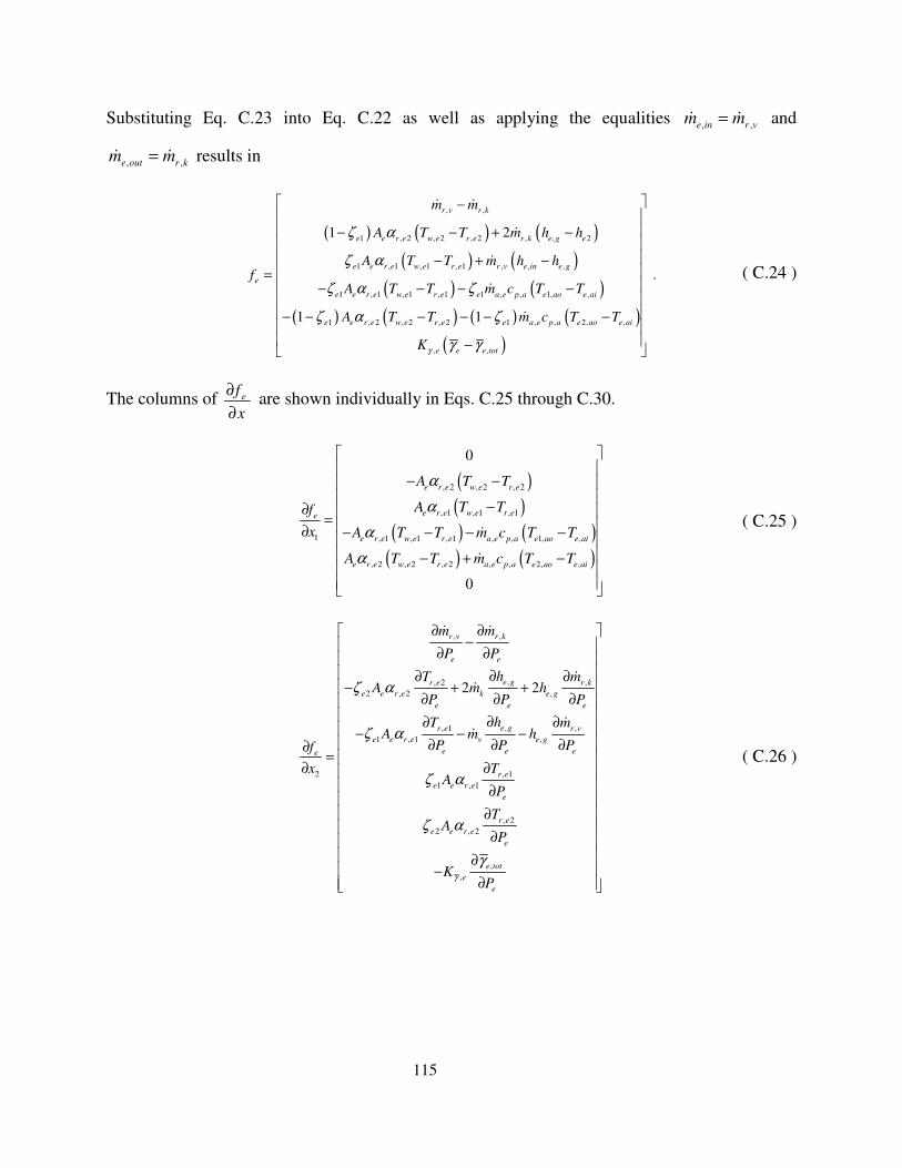
115

Substituting Eq. C.23 into Eq. C.22 as well as applying the equalities , ,e in r v

m m=ɺ ɺ and

, ,e out r km m=ɺ ɺ results in

( ) ( ) ( )

( ) ( )

( ) ( )

( ) ( ) ( ) ( )

( )

,

1 , 2 , 2 , 2 , , 2

1 , 1 , 1 , 1 ,

1 , 1 , 1 , 1 1 , 1, ,

1 , 2 , 2 , 2 1 ,

,

2, ,

, ,

, ,

,

,

1 2

1 1

r k

e e r e w e r e r k e g e

e e r e w e r e e in

e

e e r e w e r e e p a e ao e ai

e e r e w e r e e

r v

r v e g

a e

a p a e ao e ai

e e e o

e

t t

T

T

T

m m

A T m h h

A T m h hf

A T m c T

A T m

T

c TT T

Kγ

ζ α

ζ α

ζ α ζ

ζ α ζ

γ γ

− − + −

− + −=

− − − −

− − − −

−

− −

−

ɺ

ɺ

ɺ

ɺ

ɺ

ɺ .

( C.24 )

The columns of ef

x

∂

∂ are shown individually in Eqs. C.25 through C.30.

( )( )

( ) ( )( ) ( )

, 2 , 2 , 2

, 1 , 1 , 1

1 , 1 , 1 , 1 , 1, ,

, 2 , 2 , 2 , 2, ,

,

,

0

0

e r e w e r e

e r e w e r ee

e r e w e r e p a e ao e ai

e r e w e r e p a e ao e ai

a e

a e

A T T

A T T

A T T m c T T

A T T m c

f

T T

x

α

α

α

α

− −

− = − − − − −

∂

∂ −

+

ɺ

ɺ

( C.25 )

,

,, 2 ,

2 , 2 ,

,, 1

1 , 1 ,

, 1

1 , 1

, 2

2 , 2

,

2

,

,

,

2 2

r k

e e

e gr e r k

e e r e e g

e e e

e gr e

e e r e e g

e e ee

r e

e e r e

e

r e

e e r e

e

e tot

v

e

r v

k

e

r v

m m

hT mA m h

P P

hT m

P P

P

PfA m h

P P

x TA

P

K

TA

P

Pγ

ζ α

ζ α

ζ α

ζ α

γ

∂ ∂−

∂ ∂

∂

∂

∂

∂∂

∂∂ − + +

∂ ∂ ∂∂ − − − ∂ ∂

= ∂

∂ ∂

∂ ∂

∂

∂

−

ɺ ɺ

ɺɺ

ɺɺ

( C.26 )

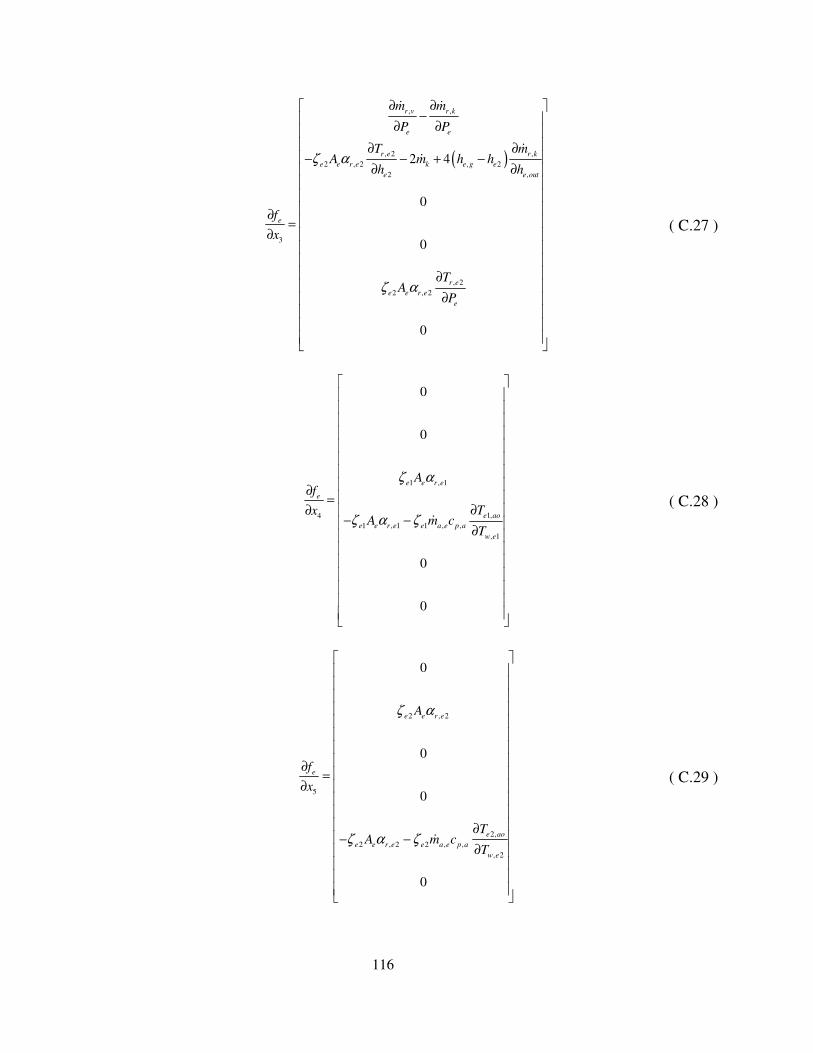
116

( )

,

, 2

, 2

2 , 2

,

, 2 ,

2 , 2

2 ,

3

2

0

4

0

0

r v

r e r k

e

r k

e e

r e

e

r e

e e r e

e

e k e g e

e e out

m m

T

P P

T mA m h h

h h

f

x

AP

ζ α

ζ α

∂ ∂−

∂ ∂

∂ ∂− − + −

∂ ∂

= ∂

∂

∂

∂

ɺ ɺ

ɺɺ

( C.27 )

1 , 1

1,

1 ,

4

1 1 ,

, 1

,

0

0

0

0

e e r e

e

e ao

ae e r e

w e

ee p a

f

x

A

TA m c

T

ζ α

ζ α ζ

=

∂ −

∂

−

∂

∂

ɺ

( C.28 )

2 , 2

2,

2 , 2 2 ,

, 2

5

,

0

0

0

0

e e r e

e

e a

a e

o

e e r e e p a

w e

A

TA m c

f

x

T

ζ α

ζ α ζ

= ∂ −

∂

∂

∂

−

ɺ

( C.29 )

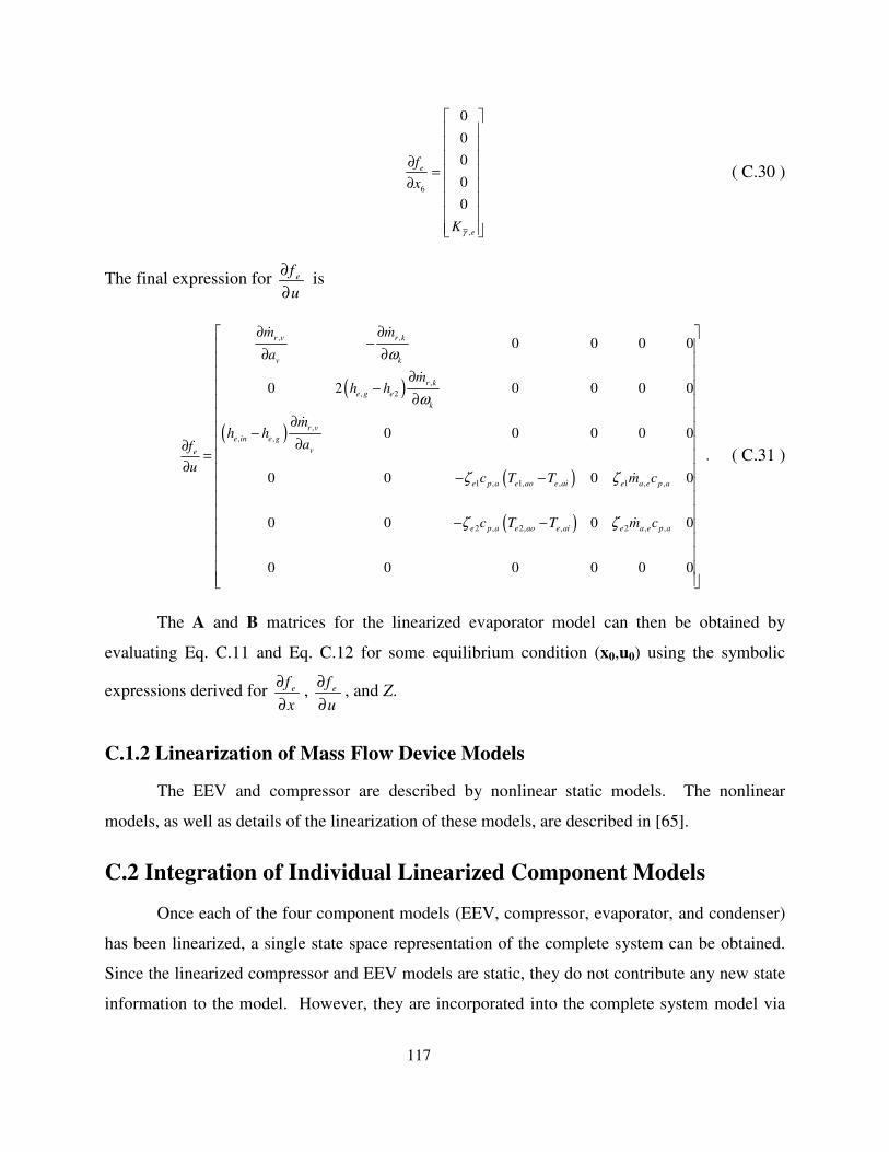
117

6

,

0

0

0

0

0

e

e

f

x

Kγ

∂

∂

=

( C.30 )

The final expression for ef

u

∂

∂ is

( )

( )

( )

( )

, ,

,

, 2

, ,

1 , 1, , 1 ,

2 , 2, , 2 ,

,

,

,

0 0 0 0

0 2 0 0 0 0

0 0 0 0 0

.

0 0 0 0

0 0 0 0

0 0 0 0 0 0

r

v k

e g e

k

e in e g

e

e p a e ao e ai e p a

e p a e a

v r k

r k

r v

v

a e

ao e ai e p ae

m m

mh

mh

c T T m c

c T T m

ha

u

c

a

h

f

ω

ω

ζ ζ

ζ ζ

∂ ∂

∂ ∂ ∂

∂ ∂ ∂∂

= ∂

−

−

−

− −

− −

ɺ ɺ

ɺ

ɺ

ɺ

ɺ

( C.31 )

The A and B matrices for the linearized evaporator model can then be obtained by

evaluating Eq. C.11 and Eq. C.12 for some equilibrium condition (x0,u0) using the symbolic

expressions derived for ef

x

∂

∂,

ef

u

∂

∂, and Z.

C.1.2 Linearization of Mass Flow Device Models

The EEV and compressor are described by nonlinear static models. The nonlinear

models, as well as details of the linearization of these models, are described in [65].

C.2 Integration of Individual Linearized Component Models

Once each of the four component models (EEV, compressor, evaporator, and condenser)

has been linearized, a single state space representation of the complete system can be obtained.

Since the linearized compressor and EEV models are static, they do not contribute any new state

information to the model. However, they are incorporated into the complete system model via

118

terms such as ,r v

v

m

a

∂

∂

ɺ which appear in the derivation of the linearized evaporator and condenser

models. After a considerable amount of algebra, symbolic expressions for the final A and B

matrices can be obtained with the following state and input vectors:

1 2 , 1 , 2 1 1 1 3 , 1 , 2 3

15

,

T

e e e w e w e e c c c c c w c w c w c cP h T P h h T T TTζ γ ζ ζ γ = ∈ x ℝ ( C.32 )

and

, , ,

6

, .T

v k a e a c e ai c aia m m T Tω = ∈ u ɺ ɺ ℝ ( C.33 )

Due to their size and complexity, the symbolic representations of A and B are not shown here.

C.3 Linearized Model Validation

The operating condition about which the system was linearized for the case study

presented in Chapter 5 is given in Eqs. C.34 and C.35.

[ ]0.860 290 256 2.32 12.2 0.979 0.148 0.688 910 295 93.5 37.0 33.7 27.7 0.852T

=0x ( C.34 )

[ ]10 1000 0.15 0.6 18 26T

=0u ( C.35 )

Note that the linearized model contains six inputs, where u0(5) and u0(6) are the evaporator and

condenser air inlet temperatures. In the optimal control problem formulation used in Chapter 5,

these two inputs are treated as disturbances because they are not controllable.

The continuous-time A and B matrices of the linearized model are shown in Eq. C.37 and

Eq. C.36 which are located at the end of this appendix because of the size of the matrices. For

the case study presented in Chapter 5, the continuous-time state space representation was

converted to discrete time with a sample time of 1 second using the c2d command in MATLAB.

The linearization is first done in continuous time because the moving boundary model governing

equations are derived in continuous time. Then for a given control methodology, the user can

choose to convert the linearized state-space representation into the most appropriate form.

The nonlinear VCC system model, simulated using the ATTMO Toolbox [66], and the

linearized model, were both perturbed using pseudo-random binary signals generated in

MATLAB. The nonlinear model inputs are shown in Figure C.1.

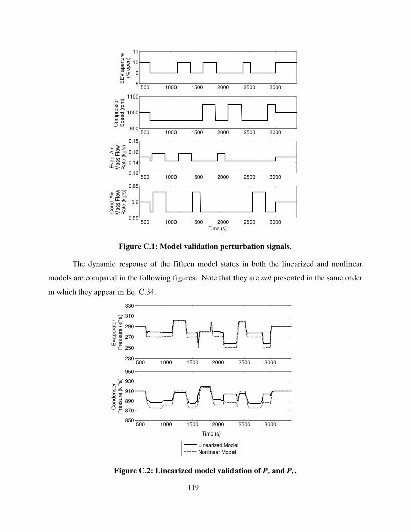
119

Figure C.1: Model validation perturbation signals.

The dynamic response of the fifteen model states in both the linearized and nonlinear

models are compared in the following figures. Note that they are not presented in the same order

in which they appear in Eq. C.34.

Figure C.2: Linearized model validation of Pc and Pe.

500 1000 1500 2000 2500 30008

9

10

11

EE

V a

pe

rtu

re

(% o

pe

n)

500 1000 1500 2000 2500 3000900

1000

1100

Co

mp

resso

rS

pe

ed

(rp

m)

500 1000 1500 2000 2500 30000.12

0.14

0.16

0.18

Eva

p. A

ir

Ma

ss F

low

Ra

te (

kg

/s)

500 1000 1500 2000 2500 30000.55

0.6

0.65

Time (s)

Co

nd

. A

ir

Ma

ss F

low

Ra

te (

kg

/s)

500 1000 1500 2000 2500 3000230

250

270

290

310

330

Eva

po

rato

r P

ressu

re (

kP

a)

500 1000 1500 2000 2500 3000850

870

890

910

930

950

Time (s)

Co

nd

en

se

r P

ressu

re (

kP

a)

Linearized Model

Nonlinear Model

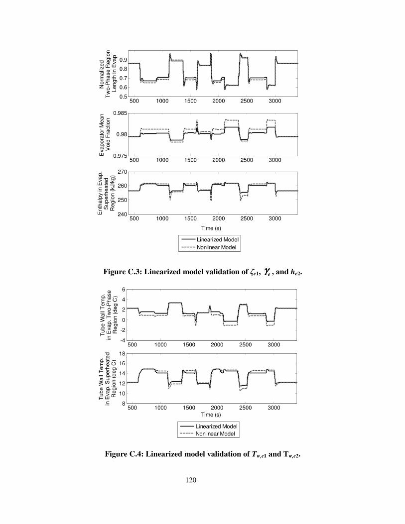
120

Figure C.3: Linearized model validation of ζe1, eγγγγ , and he2.

Figure C.4: Linearized model validation of Tw,e1 and Tw,e2.

500 1000 1500 2000 2500 30000.5

0.6

0.7

0.8

0.9

No

rma

lize

d

Tw

o-P

ha

se

Re

gio

n

Le

ng

th in

Eva

p

500 1000 1500 2000 2500 30000.975

0.98

0.985

Eva

po

rato

r M

ea

n

Vo

id F

ractio

n

500 1000 1500 2000 2500 3000240

250

260

270

Time (s)

En

tha

lpy in

Eva

p.

Su

pe

rhe

ate

d

Re

gio

n (

kJ/k

g)

Linearized Model

Nonlinear Model

500 1000 1500 2000 2500 3000-4

-2

0

2

4

6

Tu

be

Wa

ll T

em

p.

in E

va

p. T

wo

-Ph

ase

R

eg

ion

(d

eg

C)

Linearized Model

Nonlinear Model

500 1000 1500 2000 2500 30008

10

12

14

16

18

Time (s)

Tu

be

Wa

ll T

em

p.

in E

va

p. S

up

erh

ea

ted

R

eg

ion

(d

eg

C)

121

Figure C.5: Linearized model validation of ζc1, ζc2, and cγγγγ .

Figure C.6: Linearized model validation of hc1 and hc3.

500 1000 1500 2000 2500 30000

0.1

0.2

0.3

0.4

0.5

No

rma

lize

dS

up

erh

ea

ted

Re

gio

nL

en

gth

in

Co

nd

.

500 1000 1500 2000 2500 30000.5

0.6

0.7

0.8

0.9

11N

orm

alize

dT

wo

-Ph

ase

Re

gio

nL

en

gth

in

Co

nd

.

500 1000 1500 2000 2500 30000.85

0.855

0.86

Time (s)

Co

nd

ense

r M

ea

n

Vo

id F

raction

Linearized Model

Nonlinear Model

500 1000 1500 2000 2500 3000280

290

300

310

Enth

alp

y in C

on

d.

Su

pe

rhe

ate

dR

egio

n (

kJ/k

g)

500 1000 1500 2000 2500 300080

90

100

110

Time (s)

En

tha

lpy in

Co

nd

.S

ub

coo

led

Reg

ion

(kJ/k

g)

Linearized Model

Nonlinear Model

122

Figure C.7: Linearized model validation of Tw,c1, Tw,c2, and Tw,c3.

4

4

4

0.0257 4.00 0 0 0 0

4.39 0.171 0 0 0 0

1.40 0.0547 0 0 0 0

0 0 2.78 0 0.0434 0

0 0 1.03 0 0.0434 0

0.00030 0 0 0 0 0

0.0001 5.00 0 0 0 0

0.00120 6.00 0 0 0 0

0.642 0.178 0 0 0 0

0.0117 0.00320 0 0 0 0

0.00850 0

10

10

.00450 0 0 0 0

0 0 0 0.421 0 0 0

0

26

1

. 7

−

−

−

−

−

−

= −

−

−

−

−

−

×

×

×B

4

4

4.00 0.00250 0 0.293 0 0.0726

0.454 0.0030 0 0.0645 0 0.0726

1.00 0 0 0 0

10

1 00

−

−

×

×

− −

− −

( C.36 )

500 1000 1500 2000 2500 300032

34

36

38

40

42

Tu

be

Wa

ll T

em

p.

in C

on

d. S

up

erh

ea

ted

R

eg

ion

(d

eg

C)

500 1000 1500 2000 2500 300028

30

32

34

36

38

Tu

be

Wa

ll T

em

p.

in C

on

d. T

wo

-Ph

ase

R

eg

ion

(d

eg

C)

500 1000 1500 2000 2500 300024

26

28

30

32

34

Time (s)

Tu

be

Wa

ll T

em

p.

in C

on

d. S

ub

co

ole

d

Re

gio

n (

de

g C

)

Linearized Model

Nonlinear Model

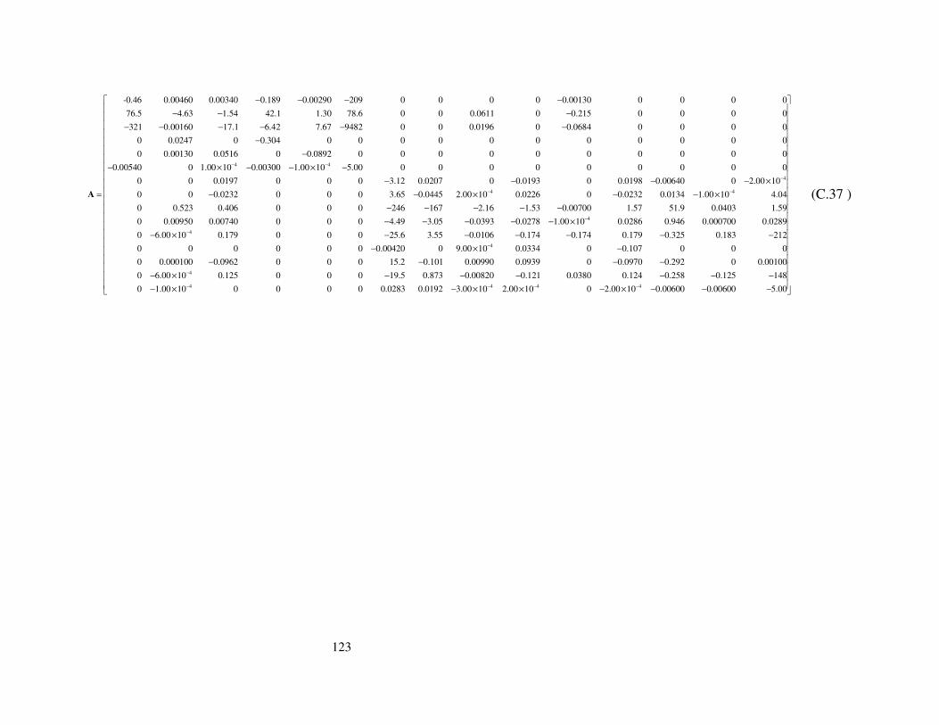
123

-0.46 0.00460 0.00340 0.189 0.00290 209 0 0 0 0 0.00130 0 0 0 0

4.63 1.54 42.1 1.30 78.6 0 0 0.0611 0 0.215 0 0 0 0

321 0.00160 17.1 6.42 7.67 9482 0 0 0.0196 0 0.0684 0 0 0 0

0 0.0247 0 0.304 0 0 0 0 0 0 0 0 0 0 0

0 0.00130 0.0516 0

76.5

0.0892 0 0

− − − −

− − −

− − − − − −

−

−

=A

4 4

4

4 4

0 0 0 0 0 0 0 0

0.00540 0 1.00 0.00300 1.00 5.00 0 0 0 0 0 0 0 0 0

0 0 0.0197 0 0 0 3.12 0.0207 0 0.0193 0 0.0198 0.00640 0 2.00

0 0 0.0232 0 0 0 3.65 0.0445 2.00 0.0226 0 0.0232 0.0134 1.00 4.04

0 0.52

10 10

10

3 0.406 0

10 1

0 0 246

0

1

− −

−

− −

× ×

×

− − − −

− −

× ×

− −

− − − −

− −4

4

67 2.16 1.53 0.00700 1.57 51.9 0.0403 1.59

0 0.00950 0.00740 0 0 0 4.49 3.05 0.0393 0.0278 1.00 0.0286 0.946 0.000700 0.0289

0 6.00 0.179 0 0 0 25.6 3.55 0.0106 0.174 0.174 0.179 0.325 0.183 212

0 0 0 0 0 0 0.00420 0 9.

1

0

0

0

1

−

−

− − −

− − − − −

− − − − − − −

−

×

×4

4

4 4

0 0.0334 0 0.107 0 0 0

0 0.000100 0.0962 0 0 0 15.2 0.101 0.00990 0.0939 0 0.0970 0.292 0 0.00100

0 6.00 0.125 0 0 0 19.5 0.873 0.00820 0.121 0.0380 0.124 0.25

10

10

10

8 0.125 148

0 1.00 0 0 0 0 0.0283 0.0192 3.00 2.010 00 1

−

−

− −

−

− − − −

− − − − − − −

×

×

× × ×− − 4 40 2.00 0.00600 0.00600 5.010 0− −

− −× − −

(C.37 )

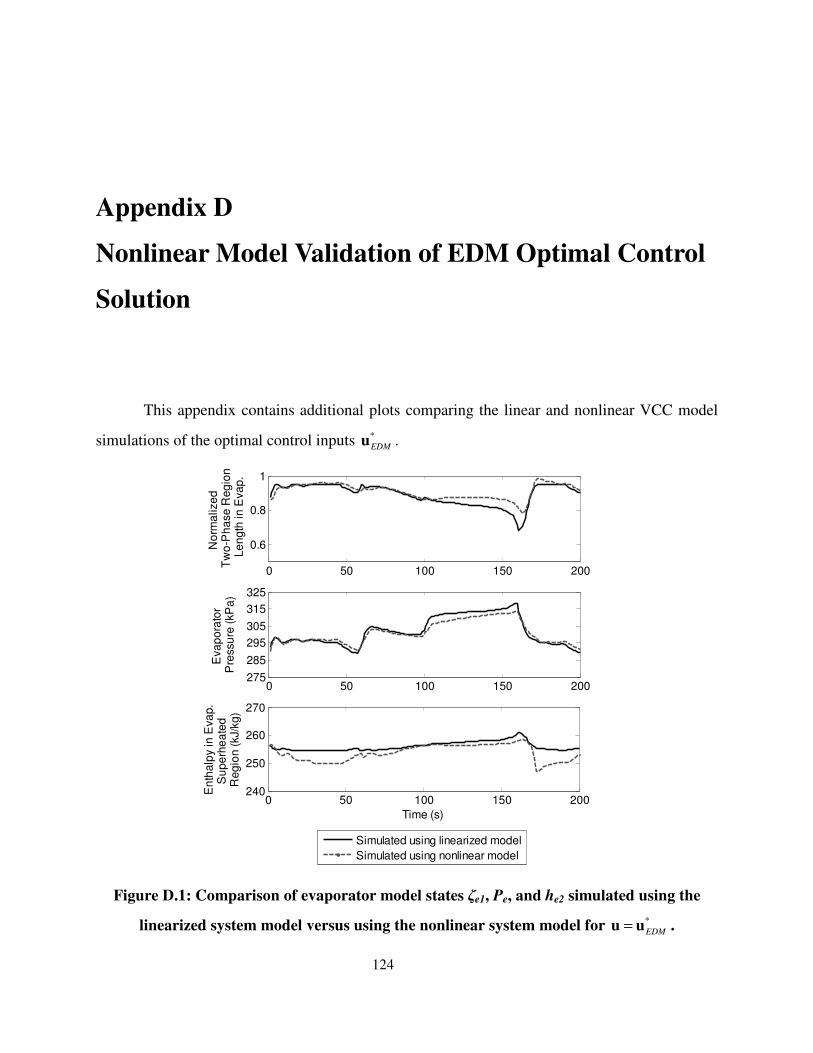
124

Appendix D

Nonlinear Model Validation of EDM Optimal Control

Solution

This appendix contains additional plots comparing the linear and nonlinear VCC model

simulations of the optimal control inputs *

EDMu .

Figure D.1: Comparison of evaporator model states ζe1, Pe, and he2 simulated using the

linearized system model versus using the nonlinear system model for *

EDM=u u .

0 50 100 150 200

0.6

0.8

1

No

rma

lize

d

Tw

o-P

ha

se R

eg

ion

Le

ngth

in

Evap

.

0 50 100 150 200275

285

295

305

315

325

Eva

pora

tor

Pre

ssu

re (

kP

a)

0 50 100 150 200240

250

260

270

Time (s)

En

thalp

y in

Eva

p.

Su

pe

rhe

ate

d

Reg

ion (

kJ/k

g)

Simulated using linearized model

Simulated using nonlinear model

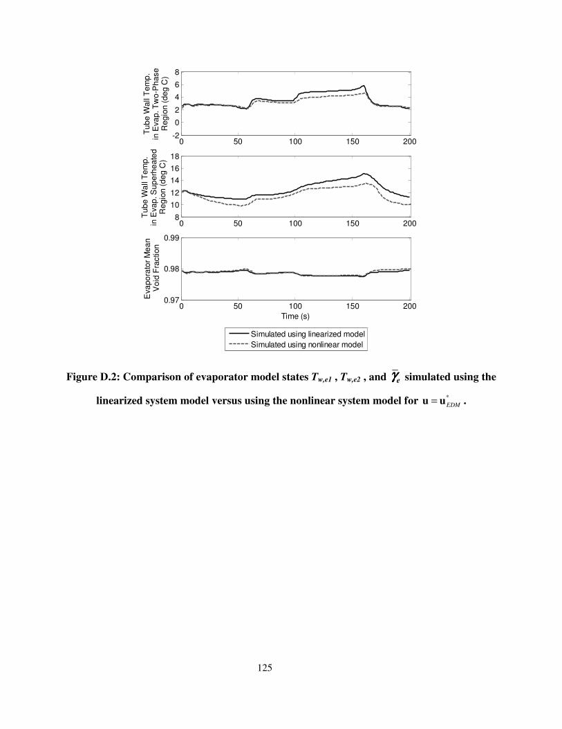
125

Figure D.2: Comparison of evaporator model states Tw,e1 , Tw,e2 , and eγγγγ simulated using the


EDM=u u .

0 50 100 150 200-2

0

2

4

6

8

Tub

e W

all T

em

p.

in E

va

p. T

wo

-Ph

ase

Re

gio

n (

de

g C

)

0 50 100 150 2008

10

12

14

16

18

Tub

e W

all T

em

p.

in E

vap

. S

up

erh

eate

d

Re

gio

n (

de

g C

)

0 50 100 150 2000.97

0.98

0.99

Time (s)

Eva

po

rato

r M

ea

n V

oid

Fra

ction



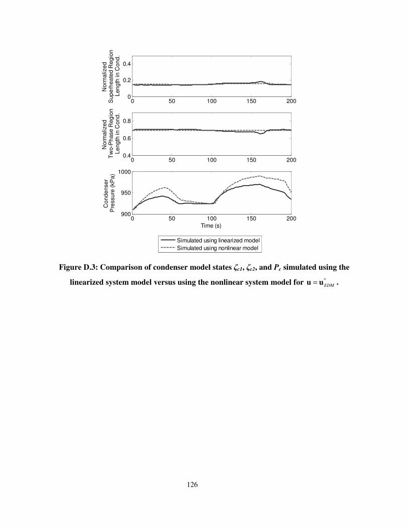
126

Figure D.3: Comparison of condenser model states ζc1, ζc2, and Pc simulated using the


EDM=u u .

0 50 100 150 2000

0.2

0.4

Norm

alize

d

Su

pe

rhea

ted R

egio

n

Len

gth

in

Con

d.

0 50 100 150 2000.4

0.6

0.8

No

rmalize

d

Tw

o-P

hase

Reg

ion

Le

ng

th in

Con

d.

0 50 100 150 200900

950

1000

Time (s)

Co

nde

nse

r P

ressu

re (kP

a)



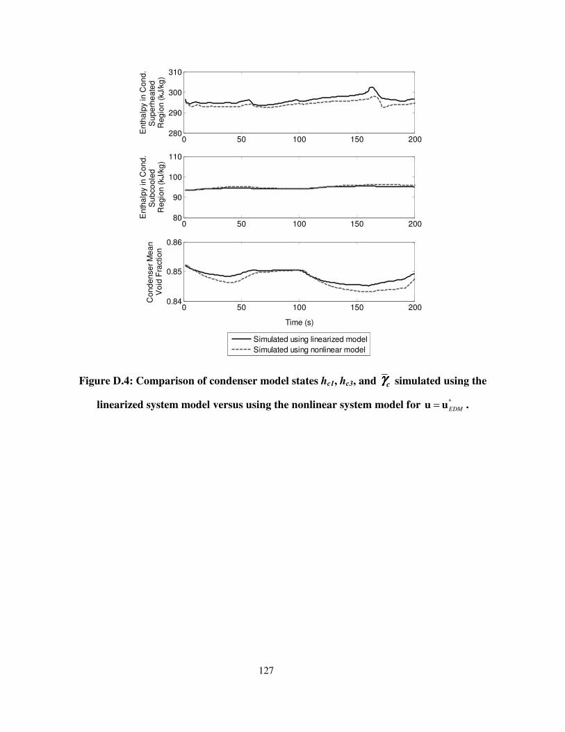
127

Figure D.4: Comparison of condenser model states hc1, hc3, and cγγγγ simulated using the


EDM=u u .

0 50 100 150 200280

290

300

310

En

tha

lpy in

Co

nd

. S

up

erh

ea

ted

R

eg

ion

(kJ/k

g)

0 50 100 150 20080

90

100

110

En

tha

lpy in

Co

nd

. S

ub

co

ole

d

Re

gio

n (

kJ/k

g)

0 50 100 150 2000.84

0.85

0.86

Time (s)

Co

nd

en

se

r M

ea

n

Vo

id F

ractio

n



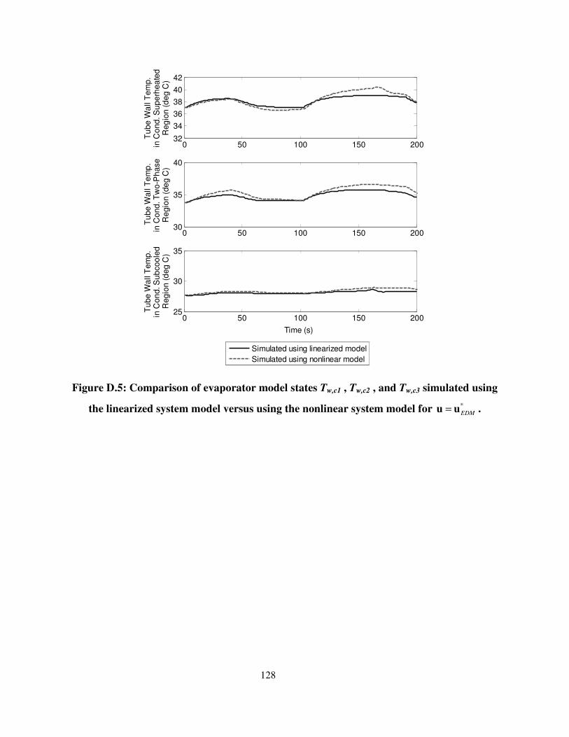
128

Figure D.5: Comparison of evaporator model states Tw,c1 , Tw,c2 , and Tw,c3 simulated using

the linearized system model versus using the nonlinear system model for *

EDM=u u .

0 50 100 150 20032

34

36

38

40

42

Tu

be

Wa

ll T

em

p.

in C

on

d. S

up

erh

ea

ted

R

eg

ion

(d

eg

C)

0 50 100 150 20030

35

40

Tu

be

Wa

ll T

em

p.

in C

on

d. T

wo

-Ph

ase

R

eg

ion

(d

eg

C)

0 50 100 150 20025

30

35

Time (s)

Tu

be

Wa

ll T

em

p.

in C

on

d. S

ub

co

ole

d

Re

gio

n (

de

g C

)



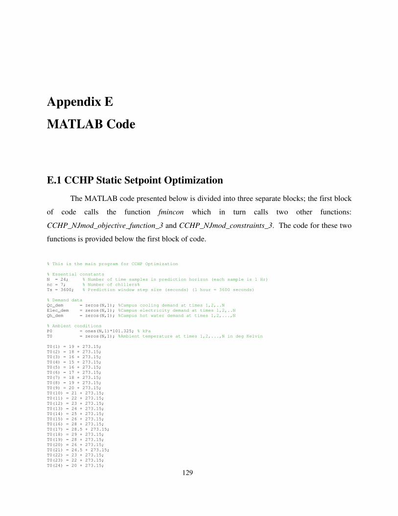
129

Appendix E

MATLAB Code

E.1 CCHP Static Setpoint Optimization

The MATLAB code presented below is divided into three separate blocks; the first block

of code calls the function fmincon which in turn calls two other functions:

CCHP_NJmod_objective_function_3 and CCHP_NJmod_constraints_3. The code for these two

functions is provided below the first block of code.

% This is the main program for CCHP Optimization

% Essential constants

N = 24; % Number of time samples in prediction horizon (each sample is 1 Hr)

nc = 7; % Number of chillers%

Ts = 3600; % Prediction window step size (seconds) (1 hour = 3600 seconds)

% Demand data

Qc_dem = zeros(N,1); %Campus cooling demand at times 1,2,..N

Elec_dem = zeros(N,1); %Campus electricity demand at times 1,2,..N

Qh_dem = zeros(N,1); %Campus hot water demand at times 1,2,...,N

% Ambient conditions

P0 = ones(N,1)*101.325; % kPa

T0 = zeros(N,1); %Ambient temperature at times 1,2,...,N in deg Kelvin

T0(1) = 19 + 273.15;

T0(2) = 18 + 273.15;

T0(3) = 16 + 273.15;

T0(4) = 15 + 273.15;

T0(5) = 16 + 273.15;

T0(6) = 17 + 273.15;

T0(7) = 18 + 273.15;

T0(8) = 19 + 273.15;

T0(9) = 20 + 273.15;

T0(10) = 21 + 273.15;

T0(11) = 22 + 273.15;

T0(12) = 23 + 273.15;

T0(13) = 24 + 273.15;

T0(14) = 25 + 273.15;

T0(15) = 26 + 273.15;

T0(16) = 28 + 273.15;

T0(17) = 28.5 + 273.15;

T0(18) = 29 + 273.15;

T0(19) = 28 + 273.15;

T0(20) = 26 + 273.15;

T0(21) = 24.5 + 273.15;

T0(22) = 23 + 273.15;

T0(23) = 22 + 273.15;

T0(24) = 20 + 273.15;

130

% Predicted campus hot water demand at times 1,2,...,N (in units of MW)

Qh_dem(1) = 1.2;

Qh_dem(2) = 1.2;

Qh_dem(3) = 1.2;

Qh_dem(4) = 1.2;

Qh_dem(5) = 1.2;

Qh_dem(6) = 5.64;

Qh_dem(7) = 5.64;

Qh_dem(8) = 4.92;

Qh_dem(9) = 4.92;

Qh_dem(10) = 4.92;

Qh_dem(11) = 3.72;

Qh_dem(12) = 3.72;

Qh_dem(13) = 2.64;

Qh_dem(14) = 2.64;

Qh_dem(15) = 2.64;

Qh_dem(16) = 2.64;

Qh_dem(17) = 5.64;

Qh_dem(18) = 5.64;

Qh_dem(19) = 5.64;

Qh_dem(20) = 5.64;

Qh_dem(21) = 4.92;

Qh_dem(22) = 4.92;

Qh_dem(23) = 1.2;

Qh_dem(24) = 1.2;

Qh_dem = 1000*Qh_dem/2.5; % Convert campus hot water demand into units of kW and scale down

%Predicted campus cooling demands at times 1,2,...N (in units of kW)

Qc_dem(1) = 26260;

Qc_dem(2) = 21883;

Qc_dem(3) = 17506;

Qc_dem(4) = 13130;

Qc_dem(5) = 13130;

Qc_dem(6) = 15318;

Qc_dem(7) = 16412;

Qc_dem(8) = 21883;

Qc_dem(9) = 26260;

Qc_dem(10) = 30637;

Qc_dem(11) = 35014;

Qc_dem(12) = 37202;

Qc_dem(13) = 39390;

Qc_dem(14) = 41579;

Qc_dem(15) = 43767;

Qc_dem(16) = 47049;

Qc_dem(17) = 0.8*49238;

Qc_dem(18) = 0.8*45955;

Qc_dem(19) = 0.8*43767;

Qc_dem(20) = 0.8*38296;

Qc_dem(21) = 32825;

Qc_dem(22) = 28448;

Qc_dem(23) = 26260;

Qc_dem(24) = 26260;

Qc_dem = Qc_dem/4.2; % Scale down hot water load

%Predicted campus electricity demands at times 1,2,...N based on real data

%in units of MW

Elec_dem(1) = 12.0;

Elec_dem(2) = 12.0;

Elec_dem(3) = 11.65;

Elec_dem(4) = 11.65;

Elec_dem(5) = 11.70;

Elec_dem(6) = 11.70;

Elec_dem(7) = 12.25;

Elec_dem(8) = 12.25;

Elec_dem(9) = 13.45;

Elec_dem(10) = 13.45;

Elec_dem(11) = 14.77;

Elec_dem(12) = 14.77;

Elec_dem(13) = 14.65;

Elec_dem(14) = 14.65;

Elec_dem(15) = 14.93;

Elec_dem(16) = 14.93;

Elec_dem(17) = 15.21;

Elec_dem(18) = 15.21;

Elec_dem(19) = 15.33;

Elec_dem(20) = 15.33;

Elec_dem(21) = 14.05;

131

Elec_dem(22) = 14.05;

Elec_dem(23) = 15.35;

Elec_dem(24) = 15.35;

Elec_dem = 1000*Elec_dem/2.5; % Convert campus electricity demand into units of kW and scale down

%*************************************************************************

%**Set Initial values to optimization variables for passing into fmincon**

%*************************************************************************

m_L_init = 9*Qc_dem/(4.18*5*(60-40)); % Initial values of mass flow rate supplied to campus at times 1,2,..N

calculated based on predicted cooling loads and design campus supply and return loads

%Initial values of overall stream mass flow rates through chillers are set

%below.

m_CHW_init(1,1) = m_L_init(1);
























m_CHW_mat_init = zeros(N,nc); % Initial values of individual chiller mass flow rates expressed as a matrix

for k = 1:N

for i = 1:nc

m_CHW_mat_init(k,i) = (m_CHW_init(k,1))/nc; % Overall stream mass flow rate uniformly distributed among

% individual chillers

end

end

T_CHWS_mat_init = ones(N,nc)*(273.15+5*(40-32)/9); % Initial values of Chiller supply water temperatures

% expressed as a matrix

m_CHW_vec_init = reshape(m_CHW_mat_init',N*nc,1); % Reshaping of initial values of individual chiller mass

% flow rates

T_CHWS_vec_init = reshape(T_CHWS_mat_init',N*nc,1); % Reshaping of initial values of individual chiller supply

% water temperatures

m_f_vec_init = ones(N,1)*0.7; % arbitrarily chosen

f_s_1_vec_init = ones(N,1)*0.5; % arbitrarily chosen

W_GT_vec_init = ones(N,1)*6000; % arbitrarily chosen

x0 = [m_CHW_vec_init; m_f_vec_init; T_CHWS_vec_init; f_s_1_vec_init; W_GT_vec_init]; %Expression for overall

% vector for initial values for passing to fmicon

%*************************************************************************

%***********************Call Optimization Solver**************************

%*************************************************************************

% Minimum mass flow permitted through each chiller

m_CHW_mat_min(1) = 1;







% Maximum mass flow permitted through each chiller

m_CHW_mat_max(1) = 88.6;




132




m_CHW_min = 5; % Minimum total water mass flow rate through chillers (not set to zero to avoid

% division by zero later on)

m_CHW_max = 1582.3; % Maximum total water mass flow rate through chillers

m_f_min = 0.2; % Minimum fuel flow rate through combustor (kg/s)

m_f_max = 0.8322; % Maximum fuel flow rate through combustor (kg/s)

f_s_1_min = 0.05; % Minimum fraction

f_s_1_max = 0.95; % Maximum fraction

T_CHWS_max = (273.15+5*(42-32)/9); %Maximum allowed temperature of overall supply stream from chillers at at

% all times

T_CHWS_min = (273.15+5*(38-32)/9); %Minimum allowed temperature of overall supply stream from chillers at at

% all times

W_GT_min = 1000; % Minimum allowed power to be generated from Gas Turbine

W_GT_max = 13500; % Maximum allowed power to be generated from Gas Turbine

% Define Upper and Lower Bound Constraints

UB = zeros(17*N,1);

LB = zeros(17*N,1);

UB(1:N) = m_CHW_mat_max(1);

UB(N+1:2*N) = m_CHW_mat_max(2);

UB(2*N+1:3*N) = m_CHW_mat_max(3);





UB(7*N+1:8*N) = m_f_max;

UB(8*N+1:9*N) = T_CHWS_max;







UB(15*N+1:16*N) = f_s_1_max;

UB(16*N+1:17*N) = W_GT_max;

LB(1:N) = m_CHW_mat_min(1);

LB(N+1:2*N) = m_CHW_mat_min(2);

LB(2*N+1:3*N) = m_CHW_mat_min(3);





LB(7*N+1:8*N) = m_f_min;

LB(8*N+1:9*N) = T_CHWS_min;







LB(15*N+1:16*N) = f_s_1_min;

LB(16*N+1:17*N) = W_GT_min;

%Perform optimization

tic;

OPTIONS =

optimset('FunValCheck','on','UseParallel','always','Display','iter','MaxFunEvals',100000000,'MaxIter',...

100000,'Algorithm','interior-point','Diagnostics','on','TolX',1e-10,'TolCon',1e-4,'TolFun',1e-10);

[x_star,fstar] =

fmincon(@CCHP_NJmod_objective_function_3,x0,[],[],[],[],LB,UB,@CCHP_NJmod_constraints_3,OPTIONS,T0,P0,Qc_dem,Qh

_dem,Elec_dem,N,nc,Ts);%xstar stores optimal variables, fstar is optimal objective function at xstar

m_CHW_mat = vec2mat(x_star(1:N*nc),nc); % (kg/s) Chilled water mass flows stored in a matrix (rows

% denote time sample (1,2,...N) and columns denote chiller number (1,2,...nc))

m_f = x_star(N*nc+1:N*nc+N); % (kg/s) Mass flow rate of fuel supplied to gas turbine at

% times 1,2,..N

T_CHWS_mat = vec2mat(x_star(N*nc+N+1:2*N*nc+N),nc);% (deg K) Chilled water supply temperatures stored in a

% matrix (rows denote time sample (1,2,...N) and columns denote chiller number (1,2,...nc))

f_s_1 = x_star(2*N*nc+N+1:2*N*nc+2*N); % (unitless) Fraction of mass flow rate diverted to steam

% turbine at times 1,2,..N

133

W_GT = x_star(2*N*nc+2*N+1:2*N*nc+3*N); % (kW) Power supplied by Gas Turbine at times 1,2,..N

T = toc

~~~~~~~~~~~~~~~~~~~~~~~~~~~~~~~~~~~~~~~~~~~~~~~~~~~~~~~~~~~~~~~~~~~~~~~~~~~~~~~~~~~~~~~~~~~~~~~~~~~~~~~~~~~~~~~~~~~~~~~~~~~

function J = CCHP_NJmod_objective_function_3(x,T0,P0,Qc_dem,Qh_dem,Elec_dem,N,nc,Ts)

% Nomenclature

% m - mass flow rate

% Q - heat transfer rate

% W - work transfer rate (power)

% T - temperature

% P - pressure

% psi - specific exergy

% ndv - number of decision variables

% np - length of prediction window

% Decision Variables

m_CHW_mat = vec2mat(x(1:N*nc),nc); % Chilled water mass flows stored in a matrix (rows denote

% time sample (1,2,...N) and columns denote chiller number (1,2,...nc))

m_f = x(N*nc+1:N*nc+N); % Mass flow rate of fuel supplied to gas turbine at times

% 1,2,..N

T_CHWS_mat = vec2mat(x(N*nc+N+1:2*N*nc+N),nc); % Chilled water supply temperatures stored in a matrix (rows


f_s_1 = x(2*N*nc+N+1:2*N*nc+2*N); % Fraction of mass flow rate diverted to steam turbine at

% times 1,2,..N

W_GT = x(2*N*nc+2*N+1:2*N*nc+3*N); % Power supplied by Gas Turbine at times 1,2,..N

% Fluid Properties (constants wrt optimization)

% Specific heat capacities (kJ/kg-K) at times 1,2,..N

c_pa = ones(N,1)*1.01; % air

c_pg = ones(N,1)*1.1; % natural gas (CH4) exhaust gas

c_pw = ones(N,1)*4.186; % water

R = 0.287*ones(N,1); % kJ/kg-K (value for air used for exhaust gas)

rho_w= 1000*ones(N,1); % kg/m^3

LHV = 50.020*1000*ones(N,1); % kJ/kg Corrected on 04/03/2013 by Neera Jain

psi_f= 51.849*1000*ones(N,1); % kJ/kg Corrected on 04/03/2013 by Neera Jain

% Operating Parameters (specified by user and constant wrt optimization)

% Pressures (kPa)

P_dae = (101.325 + 9*6.894)*ones(N,1); % Deaerator pressure in steam loop at times 1,2,..N

P_cond1 = (0.6203*101.325)*ones(N,1); % Condensor 1 pressure in steam loop at times 1,2,..N

P_w_in = (101.325 + 285*6.894)*ones(N,1); % Inlet water pressure to HRSG at times 1,2,..N

% Temperatures (deg Kelvin)

T_w_in = (5*(240-32)/9 + 273.15)*ones(N,1); % Inlet water temperatures to HRSG at times 1,2,..N in deg

% Kelvin

T_hw_sink = (5*(224-32)/9 + 273.15)*ones(N,1); % Hot water return temperature from campus hot water loop

% at times 1,2,..N in deg Kelvin

T_chwr = ( (60-32)*(5/9) + 273.15 )*ones(N,1); % 60F converted into deg Kelvin

% Enthalpy (kJ/kg)

h_w_in = 462.8*ones(N,1); % Inlet water enthalpy to HRSG in kJ/kg for specified value of P_w_in;

% 3 different cases – only one should be uncommented at any given time

% Case 1:

% Component efficiencies at times 1,2,..N

eta_compair = ones(N,1)*0.5;

eta_GT = ones(N,1)*0.5;

eta_ST = ones(N,1)*1.0;

% Case 2:


eta_compair = ones(N,1)*1.0;


eta_ST = ones(N,1)*0.5; % based on Vikas' code

% Case 0:


eta_compair = ones(N,1)*0.85; % based on data



% Other

Pr_compair = (16)*ones(N,1); % Chosen based on pressure ratio of 16 from UC Irvine slides

134

epsil = 0.8455; % HRSG overall effectiveness

f_SG_pw = 0.95; % Water stream pressure loss factor in HRSG

m_w = ( 1/1 )*( 122.6*0.001196/15.8/0.001 )*ones(N,1); % Water mass flow rate through HRSG at times

% 1,2,..N

theta_T1 = 0.0249*ones(N,1); %Defined in Eq. (22)


theta_cp1= 0.0006*ones(N,1); %Defined in Excel File created by Neera


theta_Ts1= 0.4445*ones(N,1); %Theta "Steam Temp" 1


% Control Volume 1 - Gas Turbine and Generator

m_a = ( 22.0 )*m_f; % based on non-stoichiometric combustion of methane

m_g = 1.02*m_a; % based on non-stoichiometric combustion of methane

T_air_in = T0;

T_compair_out = T_air_in.*( ones(N,1) + ( 1./eta_compair ).*( Pr_compair.^(0.4/1.4) - ones(N,1) ) ); % Units

% Kelvin

P_compair_out = P0.*Pr_compair;

W_compair = ( m_a.*c_pa.*( T_compair_out - T_air_in ) );

W_turb = W_compair + W_GT; % W_GT is the net power produced by the gas turbine; W_turb is the amount produced

% just by the turbine.

T_comb_out = ( m_f.*psi_f )./( m_a.*c_pa ) + T_compair_out;

P_comb_out = P_compair_out; % Corrected 4/3/2013 by Neera Jain

T_turb_out = T_comb_out - W_turb./( m_g.*c_pg );

P_turb_out = P_comb_out.*( ( -( 1 - T_turb_out./T_comb_out )./( eta_GT ) + 1 ).^(1.4/0.4) );

% Control Volume 2 - Heat Recovery Steam Generator (HRSG)

% Assumptions

% 1. The pressure and temperature of water exiting the steam loop ( P_w_in and T_w_in ) are controlled to be

% constant

% 2. There is no pressure drop in the gas stream from inlet to outlet ( P_g_in = P_g_out )*

% 3. The pressure in the steam/water stream drops by a constant factor f_SG_pw from inlet to outlet

T_g_in = T_turb_out; % Exhaust gas from turbine becomes inlet gas to HRSG

P_g_in = P_turb_out; % Exhaust gas from turbine becomes inlet gas to HRSG

T_g_out = T_g_in - epsil.*( T_g_in - T_w_in );

P_g_out = P_g_in; % See assumption (2)

h_s_out = h_w_in + ( m_g ./ m_w ).*c_pg.*( T_turb_out - T_g_out );

%constraint: h_s_out > hg_sat = 2797.27 kJ/kg (Tsat = 210C)

T_w_out = ( theta_Ts1.*h_s_out - theta_Ts2 ) + 273.15*ones(N,1);

P_w_out = f_SG_pw.*P_w_in;

psi_g = c_pg.*( T_g_out - T0 ) - T0.*( c_pg.*log(T_g_out./T0) - R.*log(P_g_out./P0) );

% Control Volume 3 - Steam Loop (Steam Turbine and Heating Load)

% Assumptions

% 1. The deaerator and condensers operate at constant pressures, i.e. P_cond1, P_cond2, P_dae are controlled to

% be constant

% 2. The pressure and temperature of water exiting the steam loop ( P_w_out and T_hwr ) are controlled to be

% constant

% 3. Stream driving the steam turbine behaves like an ideal gas

m_s = m_w; % The mass flow rate of water/steam is constant throughout the entire loop

m_s1 = f_s_1.*m_s;

m_s2 = m_s - m_s1;

T_s_in = T_w_out; % The hot water vapor exiting the HRSG is the steam which enters the steam loop

P_s_in = P_w_out; % The hot water vapor exiting the HRSG is the steam which enters the steam loop

T_hwr = T_w_in; % The hot water into the HRSG is the same as the hot water return wrt the steam loop

P_hwr = P_w_in; % The hot water into the HRSG is the same as the hot water return wrt the steam loop

c_ps = theta_cp1.*T_s_in + theta_cp2; %kJ/kg-K

Qh = m_s2.*c_ps.*( T_s_in - (theta_T1.*P_s_in + theta_T2) ); % The heat transferred out of the control

volume to meet the heating load

W_p1 = ( m_s1./rho_w ).*( P_dae - P_cond1 ); % Power consumed by Pump 1

W_p2 = ( m_s./rho_w ).*( P_hwr - P_dae ); % Power consumed by Pump 2

W_ST = m_s1.*c_ps.*eta_ST.*T_s_in.*( 1 - ( P_cond1./P_s_in ).^0.25 ); % Power generated by the Steam

Turbine

135

% Control Volume 4

% Assumptions

% 1. The chilled water return temperature is uniform for each chiller ( T_chwr ) and is controlled to be

% constant

% 2. The chilled water supply temperatures are allowed to vary within a small band around 40 deg F


coeff1 = [0.1357;0.1357;0.1716;0.1604;0.1213;0.3683;0.3127]; %First Regression coefficients in Eq. (2)

coeff2 = [204.91;204.91;99.453;686.29;454.94;151.29;427.63]; %Second Regression coefficients in Eq. (2)

Qc_1 = m_CHW_mat(:,1).*c_pw.*( T_chwr - T_CHWS_mat(:,1) );







W_compref1 = coeff1(1)*Qc_1 + coeff2(1)*ones(N,1);







X_d_ch_1 = (ones(N,1) - T0./T_chwr).*(Qc_1) + W_compref1;







%Objective Function – only one should be uncommented at any given time

% J - exergy

J = 0;

for k = 1:N

J = J + ( W_compair(k) - W_turb(k) + m_f(k)*psi_f(k) - m_g(k)*psi_g(k) ) + ( (1 - T0(k)/T_hwr(k))*(-Qh(k))

+ W_p1(k) + W_p2(k) - W_ST(k) ) ...

+ ( X_d_ch_1(k) + X_d_ch_2(k) + X_d_ch_3(k) + X_d_ch_4(k) + X_d_ch_5(k) + X_d_ch_6(k) + X_d_ch_7(k)

);

end

% J - exergy + energy

J = 0;

for k = 1:N

J = J + (W_compair(k) - W_turb(k) + m_f(k)*psi_f(k) - m_g(k)*psi_g(k) ) + ( (1 - T0(k)/T_hwr(k))*(-

Qh(k)) + W_p1(k) + W_p2(k) - W_ST(k) ) ...

+ ( W_compref1(k) + W_compref2(k) + W_compref3(k) + W_compref4(k) + W_compref5(k) + W_compref6(k)

+ W_compref7(k) );

end

% J - fuel

J = 0;

for k = 1:N

J = J + LHV(k)*m_f(k);

end

end

~~~~~~~~~~~~~~~~~~~~~~~~~~~~~~~~~~~~~~~~~~~~~~~~~~~~~~~~~~~~~~~~~~~~~~~~~~~~~~~~~~~~~~~~~~~~~~~~~~~~~~~~~~~~~~~~~~~~~~~~~~~

function [c,ceq] = CCHP_NJmod_constraints_3(x,T0,P0,Qc_dem,Qh_dem,Elec_dem,N,nc,Ts)

% This Function Expresses all the Equality and Inequality Constraints in the Optimization

% Nomenclature

% m - mass flow rate

% Q - heat transfer rate

% W - work transfer rate (power)

% T - temperature

% P - pressure

136

% psi - specific exergy

% ndv - number of decision variables

% np - length of prediction window

% Decision Variables

m_CHW_mat = vec2mat(x(1:N*nc),nc); % Chilled water mass flows stored in a matrix (rows denote

% time sample (1,2,...N) and columns denote chiller number (1,2,...nc))

m_f = x(N*nc+1:N*nc+N); % Mass flow rate of fuel supplied to gas turbine at times

% 1,2,..N

T_CHWS_mat = vec2mat(x(N*nc+N+1:2*N*nc+N),nc); % Chilled water supply temperatures stored in a matrix (rows


f_s_1 = x(2*N*nc+N+1:2*N*nc+2*N); % Fraction of mass flow rate diverted to steam turbine at

% times 1,2,..N

W_GT = x(2*N*nc+2*N+1:2*N*nc+3*N); % Power supplied by Gas Turbine at times 1,2,..N

% Fluid Properties (constants wrt optimization)

% Specific heat capacities (kJ/kg-K) at times 1,2,..N

c_pa = ones(N,1)*1.01; % air

c_pg = ones(N,1)*1.1; % natural gas (CH4) exhaust gas

c_pw = ones(N,1)*4.186; % water

R = 0.287*ones(N,1); % kJ/kg-K (value for air used for exhaust gas)

rho_w= 1000*ones(N,1); % kg/m^3

LHV = 50.020*1000*ones(N,1); % kJ/kg Corrected on 04/03/2013 by Neera Jain

psi_f= 51.849*1000*ones(N,1); % kJ/kg Corrected on 04/03/2013 by Neera Jain

% Operating Parameters (specified by user and constant wrt optimization)

% Pressures (kPa)

P_dae = (101.325 + 9*6.894)*ones(N,1); % Deaerator pressure in steam loop at times 1,2,..N

P_cond1 = (0.6203*101.325)*ones(N,1); % Condensor 1 pressure in steam loop at times 1,2,..N

P_w_in = (101.325 + 285*6.894)*ones(N,1); % Inlet water pressure to HRSG at times 1,2,..N

% Temperatures (deg Kelvin)

T_w_in = (5*(240-32)/9 + 273.15)*ones(N,1); % Inlet water temperatures to HRSG at times 1,2,..N in deg

% Kelvin

T_hw_sink = (5*(224-32)/9 + 273.15)*ones(N,1); % Hot water return temperature from campus hot water loop

% at times 1,2,..N in deg Kelvin

T_chwr = ( (60-32)*(5/9) + 273.15 )*ones(N,1); % 60F converted into deg Kelvin

% Enthalpy (kJ/kg)

h_w_in = 462.8*ones(N,1); % Inlet water enthalpy to HRSG in kJ/kg for specified value of P_w_in;

% Case 1:





% Case 2:





% Case 0:





% Other

Pr_compair = (16)*ones(N,1); % Chosen based on pressure ratio of 16 from UC Irvine slides

epsil = 0.8455; % HRSG overall effectiveness

f_SG_pw = 0.95; % Water stream pressure loss factor in HRSG

m_w = ( 1/1 )*( 122.6*0.001196/15.8/0.001 )*ones(N,1); % Water mass flow rate through HRSG at times

% 1,2,..N







% Control Volume 1 - Gas Turbine and Generator

m_a = ( 22.0 )*m_f; % based on non-stoichiometric combustion of methane

m_g = 1.02*m_a; % based on non-stoichiometric combustion of methane

137

T_air_in = T0;

T_compair_out = T_air_in.*( ones(N,1) + ( 1./eta_compair ).*( Pr_compair.^(0.4/1.4) - ones(N,1) ) ); % Units

Kelvin

P_compair_out = P0.*Pr_compair;

W_compair = ( m_a.*c_pa.*( T_compair_out - T_air_in ) );

W_turb = W_compair + W_GT;

T_comb_out = ( m_f.*psi_f )./( m_a.*c_pa ) + T_compair_out;

P_comb_out = P_compair_out;

T_turb_out = T_comb_out - W_turb./( m_g.*c_pg );

P_turb_out = P_comb_out.*( ( -( 1 - T_turb_out./T_comb_out )./( eta_GT ) + 1 ).^(1.4/0.4) );

% Control Volume 2 - Heat Recovery Steam Generator (HRSG)

% Assumptions

% 1. The pressure and temperature of water exiting the steam loop ( P_w_in and T_w_in ) are controlled to be

% constant

% 2. There is no pressure drop in the gas stream from inlet to outlet ( P_g_in = P_g_out )*

% 3. The pressure in the steam/water stream drops by a constant factor f_SG_pw from inlet to outlet

T_g_in = T_turb_out; % Exhaust gas from turbine becomes inlet gas to HRSG

P_g_in = P_turb_out; % Exhaust gas from turbine becomes inlet gas to HRSG

T_g_out = T_g_in - epsil.*( T_g_in - T_w_in );

P_g_out = P_g_in; % See assumption (2)

h_s_out = h_w_in + ( m_g ./ m_w ).*c_pg.*( T_turb_out - T_g_out );

%constraint: h_s_out > hg_sat = 2797.27 kJ/kg (Tsat = 210C)

T_w_out = ( theta_Ts1.*h_s_out - theta_Ts2 ) + 273.15*ones(N,1);

P_w_out = f_SG_pw.*P_w_in;

psi_g = c_pg.*( T_g_out - T0 ) - T0.*( c_pg.*log(T_g_out./T0) - R.*log(P_g_out./P0) );

% Control Volume 3 - Steam Loop (Steam Turbine and Heating Load)

% Assumptions

% 1. The deaerator and condensers operate at constant pressures, i.e. P_cond1, P_cond2, P_dae are controlled to

% be constant

% 2. The pressure and temperature of water exiting the steam loop ( P_w_out and T_hwr ) are controlled to be

% constant


m_s = m_w; % The mass flow rate of water/steam is constant throughout the entire loop

m_s1 = f_s_1.*m_s;

m_s2 = m_s - m_s1;

T_s_in = T_w_out; % The hot water vapor exiting the HRSG is the steam which enters the steam loop

P_s_in = P_w_out; % The hot water vapor exiting the HRSG is the steam which enters the steam loop

T_hwr = T_w_in; % The hot water into the HRSG is the same as the hot water return wrt the steam loop

P_hwr = P_w_in; % The hot water into the HRSG is the same as the hot water return wrt the steam loop

c_ps = theta_cp1.*T_s_in + theta_cp2; %kJ/kg-K

Qh = m_s2.*c_ps.*( T_s_in - (theta_T1.*P_s_in + theta_T2) ); % The heat transfered out of the control

volume to meet the heating load

W_p1 = ( m_s1./rho_w ).*( P_dae - P_cond1 ); % Power consumed by Pump 1

W_p2 = ( m_s./rho_w ).*( P_hwr - P_dae ); % Power consumed by Pump 2

W_ST = m_s1.*c_ps.*eta_ST.*T_s_in.*( 1 - ( P_cond1./P_s_in ).^0.25 ); % Power generated by the Steam

Turbine

% Control Volume 4

% Assumptions

% 1. The chilled water return temperature is uniform for each chiller ( T_chwr ) and is controlled to be

% constant

% 2. The chilled water supply temperatures are allowed to vary within a small band around 40 deg F


coeff1 = [0.1357;0.1357;0.1716;0.1604;0.1213;0.3683;0.3127]; %First Regression coefficients in Eq. (2)

coeff2 = [204.91;204.91;99.453;686.29;454.94;151.29;427.63]; %Second Regression coefficients in Eq. (2)






138










Qc_Total = Qc_1 + Qc_2 + Qc_3 + Qc_4 + Qc_5 + Qc_6 + Qc_7;

W_compref_Total = W_compref1 + W_compref2 + W_compref3 + W_compref4 + W_compref5 + W_compref6 + W_compref7;

%*************************************************************************

%******COOLING PLUS POWER PLANT EQUALITY AND INEQUALITY CONSTRAINTS*******

%*************************************************************************

%Equality constraints

ceq = zeros(3*N,1); %Pre-allocation for equality constraints

ceq(1:N,1) = Qc_dem - Qc_Total; % kW

ceq(N+1:2*N,1) = Qh_dem - Qh; % kW

ceq(2*N+1:3*N,1) = W_GT + W_ST - Elec_dem - W_compref_Total - (W_p1 + W_p2); % kW

%Inequality constraints

c = zeros(2*N,1);

c(1:N,1) = 2797.27*ones(N,1) - h_s_out;

c(N+1:2*N,1) = P0 - P_g_out;

end

E.2 EDM-based Optimal Control of a VCC System

The MATLAB code presented below is divided into 4 separate blocks; the first block of

code calls is an initialization script which loads various parameters to the workspace. This script

calls the function Dynamic_Optim_Exergy_R134a_Offline which in turn calls two other

functions: Dynamic_Solver_Exergy_R134a_offline, Dynamic_Nonlcon_Exergy_R134a_offline.

% Initialization File for Offline Optimization

clear all;clc;

%Updated 11-23-12

load dnom_112312

load xnom_112312

load unom_112312

X0 = xnom;

U0 = unom;

Ts = 1; % sampling time

nu = 200; % control horizon

np = 200; % prediction horizon

n = 15; % number of states

u = 4; % number of control inputs

nd = 2; % number of disturbances

%% Load Desired Capacity and Ambient Temperature Profiles

load C_des_400_pt_84_2

C_des = C_desired(1:200);

T_H = ones(np,1)*26;

139

T_L = ones(np,1)*18;

%% Define optim_input

optim_input = [X0; U0; xnom; unom; dnom];

clear xnom unom dnom X0 U0 C_desired

%% Load Heat Transfer Coefficients

load UA_values_112312

U_guess = zeros(u*np,1);

%% Load System Model

A = eye(n);

B1 = zeros(n,u);

B2 = zeros(n,nd);

load VCC_A_matrix_discrete_point83_nonIScomp_TS1

load VCC_B1_matrix_discrete_point83_nonIScomp_TS1

load VCC_B2_matrix_discrete_point83_nonIScomp_TS1

% Load these but they will not be used

load E_matrix

load D_matrix

D_matrix = D;

E_matrix = E;

A = VCC_A;

B1 = VCC_B1;

B2 = VCC_B2;

clear VCC_A VCC_B1 VCC_B2

%% Define Max and Min bounds on U

Mins = [8; 900; 0.10; 0.30];

Maxs = [11; 1100; 0.3; 0.65];

%%

output = Dynamic_Optim_Exergy_R134a_Offline(optim_input, C_des, T_L, T_H, Ts, nu, np, n, u, nd, UA, A, B1, B2,

D_matrix, E_matrix, Mins, Maxs, U_guess)

~~~~~~~~~~~~~~~~~~~~~~~~~~~~~~~~~~~~~~~~~~~~~~~~~~~~~~~~~~~~~~~~~~~~~~~~~~~~~~~~~~~~~~~~~~~~~~~~~~~~~~~~~~~~~~~~~~~~~~~~~~~

function [output] = Dynamic_Optim_Exergy_R134a_Offline(optim_input, C_des, T_L, T_H, Ts, nu, np, n, u, nd, UA,

A, B1, B2, D_matrix, E_matrix, Mins, Maxs, U_guess)

tic;

X0 = optim_input(1:15); % absolute X0

U0 = optim_input(16:19); % absolute U0

xnom = optim_input(20:34); % nominal x

unom = optim_input(35:38); % nominal u

dnom = optim_input(39:40); % nominal d

% Create lifted nominal vectors for U, X, and D

Unom_Lifted = zeros(nu*u,1);

for i = 1:u:u*nu

Unom_Lifted(i:i+u-1) = unom;

end

clear i

Xnom_Lifted = zeros(np*n,1);

for i = 1:n:n*np

Xnom_Lifted(i:i+n-1) = xnom;

end

clear i

Dnom_Lifted = zeros(np*nd,1);

for i = 1:nd:nd*np

Dnom_Lifted(i:i+nd-1) = dnom;

end

clear i

140

% Create lifted D and D_delta vectors

D = zeros(np*nd,1);

k = 1;

for i = 1:nd:nd*np

D(i:i+nd-1) = [T_L(k); T_H(k)];

k = k + 1;

end

clear i k

D_delta = D - Dnom_Lifted;

% Define Augmented x vector (not lifted yet)

X0_delta = X0 - xnom;

U0_delta = U0 - unom;

X_bar0_delta = [X0_delta;U0_delta];

% State Space System Representation

C1 = eye(n);

C2 = eye(u);

% Define Augmented System [x x_u]

A_bar = [A B1; zeros(u,n) eye(u)];

B1_bar = [B1;eye(u)];

B2_bar = [B2;zeros(u,nd)];

% c_bar = [C1 zeros(n,u); zeros(u,n) C2];

c_bar = [C1 zeros(n,u)];

c2_bar = [zeros(u,n) C2];

C_bar = zeros(n*np,(n+u)*np);

for i = 1:np

C_bar((i-1)*n+1:i*n,(i-1)*(n+u)+1:i*(n+u)) = c_bar;

end

C2_bar = zeros(u*np, (n+u)*np);

for i = 1:np

C2_bar((i-1)*u+1:i*u,(i-1)*(n+u)+1:i*(n+u)) = c2_bar;

end

% Define Lifted Matrices for Determining X_bar

T = zeros((n+u)*np,n+u);

for i = 1:np

T((i-1)*(n+u)+1:i*(n+u),:) = A_bar^i;

end

S1 = zeros((n+u)*np,u*nu);

for i = 1:np

for j = 1:nu

if i-j < 0

S1((i-1)*(n+u)+1:i*(n+u),(j-1)*u+1:j*u) = zeros((n+u),u);

elseif i-j == 0

S1((i-1)*(n+u)+1:i*(n+u),(j-1)*u+1:j*u) = B1_bar;

elseif i-j > 0

S1((i-1)*(n+u)+1:i*(n+u),(j-1)*u+1:j*u) = A_bar^(i-j)*B1_bar;

end

end

end

S2 = zeros((n+u)*np,nd*np);

for i = 1:np

for j = 1:nu

if i-j < 0

S2((i-1)*(n+u)+1:i*(n+u),(j-1)*nd+1:j*nd) = zeros((n+u),nd);

elseif i-j == 0

S2((i-1)*(n+u)+1:i*(n+u),(j-1)*nd+1:j*nd) = B2_bar;

elseif i-j > 0

S2((i-1)*(n+u)+1:i*(n+u),(j-1)*nd+1:j*nd) = A_bar^(i-j)*B2_bar;

end

end

end

% Define Matrices for Linear Constraints

141

% Linear constraints on 'Zeta_e1' and 'Zeta_c1+Zeta_c2'

m = zeros(2,n);

m(1,1) = 1;

m(2,7) = 1;

m(2,8) = 1;

M = zeros(2*np,n*np);

for i = 1:np

M((i-1)*2+1:i*2,(i-1)*n+1:i*n) = m;

end

zmax = [(1-0.05);(1-0.05)];

znom = [xnom(1);(xnom(7)+xnom(8))];

Zmax = zeros(2*np,1);

Znom = zeros(2*np,1);

for i = 1:np

Zmax((i-1)*2+1:i*2) = zmax;

Znom((i-1)*2+1:i*2) = znom;

end

bZETAmax = (Zmax - Znom) - M*C_bar*T*X_bar0_delta - M*C_bar*S2*D_delta;

aZETAmax = M*C_bar*S1;

clear M m znom zmax Znom Zmax

% Linear constraints on 'Tw3c'

m = zeros(1,n);

m(1,14) = 1;

M = zeros(1*np,n*np);

for i = 1:np

M((i-1)*1+1:i*1,(i-1)*n+1:i*n) = m;

end

Zmax = T_H + 0.2;

znom = [xnom(14)];

Znom = zeros(1*np,1);

for i = 1:np

Znom((i-1)*1+1:i*1) = znom;

end

bTwmax = -Zmax + Znom + M*C_bar*T*X_bar0_delta + M*C_bar*S2*D_delta;

aTwmax = -M*C_bar*S1;

% Upper and Lower Bound Constraints on U

bmin = zeros(u*nu,1);

for i = 1:nu;

bmin((i-1)*u+1:i*u,1) = -Mins+U0;

end

bmax = zeros(u*nu,1);

for i = 1:nu;

bmax((i-1)*u+1:i*u,1) = Maxs-U0;

end

amin = zeros(u*nu);

for i = 1:nu

for j = 1:nu

if i-j >= 0

amin((i-1)*u+1:i*u,(j-1)*u+1:j*u)=-1*eye(u);

else

amin((i-1)*u+1:i*u,(j-1)*u+1:j*u)=zeros(u);

end

end

end

amax = zeros(u*nu);

for i = 1:nu

for j = 1:nu

if i-j >= 0

amax((i-1)*u+1:i*u,(j-1)*u+1:j*u)=eye(u);

else

amax((i-1)*u+1:i*u,(j-1)*u+1:j*u)=zeros(u);

end

end

end

a = [amin;amax;aZETAmax;aTwmax];

b = [bmin;bmax;bZETAmax;bTwmax];

142

%%%%%%%%%%%%%%%%%%%%%%%%%%%%%%%%%%%%%%%%%%%%%%%%%%%%%%%%%%%%%%%%%%%%%%%%%%%

% Stage 2: Optimization

%%%%%%%%%%%%%%%%%%%%%%%%%%%%%%%%%%%%%%%%%%%%%%%%%%%%%%%%%%%%%%%%%%%%%%%%%%%

I_L = amax;

OPTIONS =

optimset('FunValCheck','on','UseParallel','always','Display','iter','MaxFunEvals',2000000,'MaxIter',...

2000000,'Algorithm','sqp','Diagnostics','on','TolX',1e-3,'TolCon',5e-4,'TolFun',1e-3);

% Call FMINCON

[U,J_fval,Exitflag] = fmincon(@Dynamic_Solver_Exergy_R134a_offline,U_guess,a,b,[],[],[],[],...

@Dynamic_Nonlcon_Exergy_R134a_offline,OPTIONS,T,S1,S2,X0_delta,U0_delta,D_delta,Xnom_Lifted,Unom_Lifted,C_bar,C

2_bar,C_des,T_L,T_H,Ts,nu,np,n,u,nd,I_L,UA,D_matrix,E_matrix);

T = toc

%%%%%%%%%%%%%%%%%%%%%%%%%%%%%%%%%%%%%%%%%%%%%%%%%%%%%%%%%%%%%%%%%%%%%%%%%%%

% Stage 3: Create output vector

%%%%%%%%%%%%%%%%%%%%%%%%%%%%%%%%%%%%%%%%%%%%%%%%%%%%%%%%%%%%%%%%%%%%%%%%%%%

output = [U; J_fval; Exitflag; T];

end

~~~~~~~~~~~~~~~~~~~~~~~~~~~~~~~~~~~~~~~~~~~~~~~~~~~~~~~~~~~~~~~~~~~~~~~~~~~~~~~~~~~~~~~~~~~~~~~~~~~~~~~~~~~~~~~~~~~~~~~~~~~

function J =

Dynamic_Solver_Exergy_R134a_offline(U,T,S1,S2,X0_delta,U0_delta,D_delta,Xnom_Lifted,Unom_Lifted,C_bar,C2_bar,C_

des,T_L,T_H,Ts,nu,np,n,u,nd,I_L,UA,D_matrix,E_matrix)

load FluidProp_R134a_Thermosys

% Assign values to physical parameters of HX's

L_ref_e = 11.45;

Ac_ref_e = 5.165e-5;

L_ref_c = 10.6895;

Ac_ref_c = 5.156e-5;

% Convert T_H and T_L to Kelvin

Tcai_K = T_H + ones(np,1)*273;

Teai_K = T_L + ones(np,1)*273;

% Initial State Vector - X0_delta (dimension: 15 x 1) - delta away from nominal

% Initial Input Vector - U0_delta (dimension: 4 x 1) - delta away from nominal

% Define X_bar0


X_bar_delta = T*X_bar0_delta + S1*U + S2*D_delta; % delta away from nominal

X_delta = C_bar*X_bar_delta; % (separating X from X_bar)

Xu_delta = C2_bar*X_bar_delta; % (separating Xu from X_bar)

X = X_delta + Xnom_Lifted; % column vector of states

X_0 = X0_delta + Xnom_Lifted(1:n); % column vector

% Separate lifted state vector X_bar into individual state sequences:

zeta_e1 = zeros(np+1,1);

Pe = zeros(np+1,1);

He2 = zeros(np+1,1);

Tw1e = zeros(np+1,1);


GammaE = zeros(np+1,1);

zeta_c1 = zeros(np+1,1);


Pc = zeros(np+1,1);

Hc1 = zeros(np+1,1);


Tw1c = zeros(np+1,1);



GammaC = zeros(np+1,1);

i = 1;

zeta_e1(i) = X_0(1);

143

Pe(i) = X_0(2);

He2(i) = X_0(3);

Tw1e(i) = X_0(4);

Tw2e(i) = X_0(5);

GammaE(i) = X_0(6);

zeta_c1(i) = X_0(7);

zeta_c2(i) = X_0(8);

Pc(i) = X_0(9);

Hc1(i) = X_0(10);

Hc3(i) = X_0(11);

Tw1c(i) = X_0(12);

Tw2c(i) = X_0(13);

Tw3c(i) = X_0(14);

GammaC(i) = X_0(15);

clear i

zeta_e1(2:end) = X(1:n:end);

Pe(2:end) = X(2:n:end);

He2(2:end) = X(3:n:end);

Tw1e(2:end) = X(4:n:end);


GammaE(2:end) = X(6:n:end);

zeta_c1(2:end) = X(7:n:end);


Pc(2:end) = X(9:n:end);

Hc1(2:end) = X(10:n:end);


Tw1c(2:end) = X(12:n:end);



GammaC(2:end) = X(15:n:end);

zeta_e2 = ones(np+1,1) - zeta_e1;

zeta_c3 = ones(np+1,1) - zeta_c1 - zeta_c2;

U0_Lifted = zeros(np*u,1);

U_MPC = U0_Lifted + I_L*U + Unom_Lifted;

a_v = zeros(np,1);

omega_k = zeros(np,1);

me_air = zeros(np,1);

mc_air = zeros(np,1);

a_v = U_MPC(1:u:end);

omega_k = U_MPC(2:u:end);

me_air = U_MPC(3:u:end);

mc_air = U_MPC(4:u:end);

U_MPC2 = U0_Lifted + I_L*U + Unom_Lifted;

omega_k2 = U_MPC2(2:u:end);

%%%%%%%%%%%%%%%%%%%%%%%%%%%%%%%%%%%%%%%%%%%%%%%%%%%%%%%%%%%%%%%%%%%%%%%%%%%

%%%%%%%%%%%%%%%%%%%%%%%%%%%%%%%%%%%%%%%%%%%%%%%%%%%%%%%%%%%%%%%%%%%%%%%%%%%

% Determing necessary refrigerant properties via interpolation

% Evaporator

% Two-Phase Zone (Evaporator)

Tr1e = interp1(FluidProp.Psat, FluidProp.Tsat, Pe);

H1g = interp1(FluidProp.Psat, FluidProp.Hg, Pe);

rho1g = interp1(FluidProp.Psat, FluidProp.Rhog, Pe);

rho1f = interp1(FluidProp.Psat, FluidProp.Rhof, Pe);

drho1g_dP = interp1(FluidProp.Psat, FluidProp.dRhog_dP, Pe);

drho1f_dP = interp1(FluidProp.Psat, FluidProp.dRhof_dP, Pe);

rho_e1 = GammaE.*rho1g+(ones(np+1,1)-GammaE).*rho1f;

drho_e1_dP = GammaE.*drho1g_dP+(ones(np+1,1)-GammaE).*drho1f_dP;

s1g = interp1(FluidProp.Psat, FluidProp.sg, Pe);

s1f = interp1(FluidProp.Psat, FluidProp.sf, Pe);

ds1g_dP = interp1(FluidProp.Psat, FluidProp.dsg_dP, Pe);

ds1f_dP = interp1(FluidProp.Psat, FluidProp.dsf_dP, Pe);

xbar_e = (rho1g./rho_e1).*GammaE;

s_e1 = xbar_e.*s1g+(ones(np+1,1)-xbar_e).*s1f;

ds1_dGamma_P = ((GammaE.*rho1g + (ones(np+1,1)-GammaE).*rho1f).*(rho1g.*s1g - rho1f.*s1f) - ...

144

(GammaE.*rho1g.*s1g + rho1f.*s1f - GammaE.*rho1f.*s1f).*(rho1g - rho1f))./((GammaE.*rho1g + (ones(np+1,1)-

GammaE).*rho1f).^2);

ds1_dP_Gamma = (rho_e1.*((GammaE.*rho1g.*ds1g_dP + GammaE.*s1g.*drho1g_dP)+(rho1g.*ds1f_dP +

s1f.*drho_e1_dP)+...

(GammaE.*rho1g.*ds1f_dP + GammaE.*s1f.*drho1g_dP)) - (GammaE.*rho1g.*s1g + rho_e1.*s1f -

GammaE.*rho1g.*s1f).*drho_e1_dP) ./ (rho_e1.^2);

% Superheated Zone (Evaporator)

Tr2e = interp2(FluidProp.H, FluidProp.P, FluidProp.T_ph, He2, Pe);

rho_e2 = interp2(FluidProp.H, FluidProp.P, FluidProp.Rho_ph, He2, Pe);

s_e2 = interp2(FluidProp.H, FluidProp.P, FluidProp.S_ph, He2, Pe);

ds2_dH_P = interp2(FluidProp.H, FluidProp.P, FluidProp.dS_dH_P_ph, He2, Pe);

ds2_dP_H = interp2(FluidProp.H, FluidProp.P, FluidProp.dS_dP_H_ph, He2, Pe);

drho2_dH_P = interp2(FluidProp.H, FluidProp.P, FluidProp.dRho_dH_P_ph, He2, Pc);

drho2_dP_H = interp2(FluidProp.H, FluidProp.P, FluidProp.dRho_dP_H_ph, He2, Pc);

He_out = 2.*He2 - H1g;

s_k_in = interp2(FluidProp.H, FluidProp.P, FluidProp.S_ph, He_out, Pe);

Xe = GammaE.*(rho1g./rho_e1);

%%%%%%%%%%%%%%%%%%%%%%%%%%%%%%%%%%%%%%%%%%%%%%%%%%%%%%%%%%%%%%%%%%%%%%%%%%%

% Calculate valve mass flow rate

Pdelta = Pc(2:np+1)-Pe(2:np+1);

Cd = (-9.5984e-6) + (2.0481e-6).*a_v + (5.4106e-9).*Pdelta + (-7.4909e-10).*a_v.*Pdelta + ...

(-3.7775e-8).*(a_v.^2);

rho_c3 = interp2(FluidProp.H, FluidProp.P, FluidProp.Rho_ph, Hc3, Pc);

mdot_v = zeros(np+1,1);

mdot_v(2:np+1) = Cd.*sqrt(rho_c3(2:np+1).*Pdelta);

% Calculate compressor mass flow rate

rho_k_in = interp2(FluidProp.H_mg_ph,FluidProp.P_mg_ph,FluidProp.Rho_ph,He_out,Pe);

rps = omega_k./60;

P_ratio = Pc(2:np+1)./Pe(2:np+1);

eta_v = 0.65127 + 0.00027681.*omega_k - 0.031338.*P_ratio + 3.0221e-5.*omega_k.*P_ratio...

- 1.1905e-7.*(omega_k.^2) - 0.0081256.*(P_ratio.^2);

volume = 3.042e-5;

mdot_k = zeros(np+1,1);

mdot_k(2:np+1)= rps.*volume.*rho_k_in(2:np+1).*eta_v;

Hk_out_s = interp2(FluidProp.S, FluidProp.P, FluidProp.H_ps, s_k_in, Pc);

eta_is = ( (0.054812149750754) + (0.220895407941643).*P_ratio + (0.000034670672050).*omega_k2.*P_ratio +

...

(-0.000000036818854).*omega_k2.^2 + (-0.041677058377446).*P_ratio.^2 );

Hk_out(2:np+1)= (Hk_out_s(2:np+1) - He_out(2:np+1))./eta_is + He_out(2:np+1);

Hc_in(2:np+1) = Hk_out(2:np+1);

H2g = interp1(FluidProp.Psat, FluidProp.Hg, Pc);

Hc1(2:np+1) = 0.5*(H2g(2:np+1) + Hc_in(2:np+1)');

s_k_out(2:np+1) = interp2(FluidProp.H, FluidProp.P, FluidProp.S_ph, Hc_in(2:np+1)', Pc(2:np+1));

%%%%%%%%%%%%%%%%%%%%%%%%%%%%%%%%%%%%%%%%%%%%%%%%%%%%%%%%%%%%%%%%%%%%%%%%%%%


% Condenser

% Superheated Zone (Condenser)

Tr1c = interp2(FluidProp.H, FluidProp.P, FluidProp.T_ph, Hc1, Pc);


s_c1 = interp2(FluidProp.H, FluidProp.P, FluidProp.S_ph, Hc1, Pc);

ds1_dH_P = interp2(FluidProp.H, FluidProp.P, FluidProp.dS_dH_P_ph, Hc1, Pc);

ds1_dP_H = interp2(FluidProp.H, FluidProp.P, FluidProp.dS_dP_H_ph, Hc1, Pc);

drho1_dH_P = interp2(FluidProp.H, FluidProp.P, FluidProp.dRho_dH_P_ph, Hc1, Pc);

drho1_dP_H = interp2(FluidProp.H, FluidProp.P, FluidProp.dRho_dP_H_ph, Hc1, Pc);

% Two-Phase Zone (Condenser)

Tr2c = interp1(FluidProp.Psat, FluidProp.Tsat, Pc);

H2f = interp1(FluidProp.Psat, FluidProp.Hf, Pc);

rho2g = interp1(FluidProp.Psat, FluidProp.Rhog, Pc);

rho2f = interp1(FluidProp.Psat, FluidProp.Rhof, Pc);

drho2g_dP = interp1(FluidProp.Psat, FluidProp.dRhog_dP, Pc);

drho2f_dP = interp1(FluidProp.Psat, FluidProp.dRhof_dP, Pc);

rho_c2 = GammaC.*rho2g+(ones(np+1,1)-GammaC).*rho2f;

drho_c2_dP = GammaC.*drho2g_dP+(ones(np+1,1)-GammaC).*drho2f_dP;

145

s2g = interp1(FluidProp.Psat, FluidProp.sg, Pc);

s2f = interp1(FluidProp.Psat, FluidProp.sf, Pc);

ds2g_dP = interp1(FluidProp.Psat, FluidProp.dsg_dP, Pc);

ds2f_dP = interp1(FluidProp.Psat, FluidProp.dsf_dP, Pc);

xbar_c = (rho2g./rho_c2).*GammaC;

s_c2 = xbar_c.*s2g+(ones(np+1,1)-xbar_c).*s2f;

ds2_dGamma_P = ((GammaC.*rho2g + (ones(np+1,1)-GammaC).*rho2f).*(rho2g.*s2g - rho2f.*s2f) - ...

(GammaC.*rho2g.*s2g + rho2f.*s2f - GammaC.*rho2f.*s2f).*(rho2g - rho2f))./((GammaC.*rho2g + (ones(np+1,1)-

GammaC).*rho2f).^2);

ds2_dP_Gamma = (rho_c2.*((GammaC.*rho2g.*ds2g_dP + GammaC.*s2g.*drho2g_dP)+(rho2g.*ds2f_dP +

s2f.*drho_c2_dP)+...

(GammaC.*rho2g.*ds2f_dP + GammaC.*s2f.*drho2g_dP)) - (GammaC.*rho2g.*s2g + rho_c2.*s2f -

GammaC.*rho2g.*s2f).*drho_c2_dP) ./ (rho_c2.^2);

Xc = GammaC.*(rho2g./rho_c2);

% Subcooled Zone (Condenser)





Hc_out = 2.*Hc3 - H2f;


%%%%%%%%%%%%%%%%%%%%%%%%%%%%%%%%%%%%%%%%%%%%%%%%%%%%%%%%%%%%%%%%%%%%%%%%%%%

Ae_i = 0.29166; %m^2

Ac_i = 0.275; %m^2

UAe1 = (UA(1)*Ae_i).*zeta_e1;


UAc1 = (UA(4)*Ac_i).*zeta_c1;



Tw1e_k = Tw1e + ones(np+1,1)*273;

Tw2e_k = Tw2e + ones(np+1,1)*273;

Tw1c_k = Tw1c + ones(np+1,1)*273;

Tw2c_k = Tw2c + ones(np+1,1)*273;

Tw3c_k = Tw3c + ones(np+1,1)*273;

%%%%%%%%%%%%%%%%%%%%%%%%%%%%%%%%%%%%%%%%%%%%%%%%%%%%%%%%%%%%%%%%%%%%%%%%%%%

%%%%%%%%%%%%%%%%%%%%%%%%%%%%%%%%%%%%%%%%%%%%%%%%%%%%%%%%%%%%%%%%%%%%%%%%%%%

% Evaluating J_VCC (first for-loop calculates exergy based cost function and second for-loop calculates energy

based cost function; only evaluate one at a time)

% Initialize SUM

SUM = 0; % scalar

delta_t = Ts;

for i = 2:np+1

% Condenser Entropy Terms

mc_12 = mdot_k(i) - L_ref_c*Ac_ref_c*( ( rho_c1(i) - rho2g(i) )*( zeta_c1(i)-zeta_c1(i-1) )/delta_t +

zeta_c1(i)*drho1_dP_H(i)*( Pc(i)-Pc(i-1) )/delta_t ...

+ zeta_c1(i)*drho1_dH_P(i)*( Hc1(i)-Hc1(i-1) )/delta_t );

mc_23 = mdot_v(i) + L_ref_c*Ac_ref_c*( rho2f(i) - rho_c3(i) )*( ( zeta_c1(i)-zeta_c1(i-1) )/delta_t + (

zeta_c2(i)-zeta_c2(i-1) )/delta_t ) ...

+ L_ref_c*Ac_ref_c*zeta_c3(i)*drho3_dH_P(i)*( Hc3(i)-Hc3(i-1) )/delta_t;

dmc1_dt = ( mdot_k(i) - mc_12 ) + L_ref_c*Ac_ref_c*rho2g(i)*( ( zeta_c1(i)-zeta_c1(i-1) )/delta_t );

dmc2_dt = ( mc_12 - mc_23 ) + L_ref_c*Ac_ref_c*rho2f(i)*( ( zeta_c1(i)-zeta_c1(i-1) )/delta_t + (

zeta_c2(i)-zeta_c2(i-1) )/delta_t ) - ...

L_ref_c*Ac_ref_c*rho2g(i)*( ( zeta_c1(i)-zeta_c1(i-1) )/delta_t );

dmc3_dt = ( mc_23 - mdot_v(i) ) - L_ref_c*Ac_ref_c*rho2f(i)*( ( zeta_c1(i)-zeta_c1(i-1) )/delta_t + (

zeta_c2(i)-zeta_c2(i-1) )/delta_t );

Term_2 = s_c1(i)*dmc1_dt + L_ref_c*Ac_ref_c*rho_c1(i)*zeta_c1(i)*( ds1_dH_P(i)*( Hc1(i)-Hc1(i-1)

)/delta_t + ds1_dP_H(i)*( Pc(i)-Pc(i-1) )/delta_t );

Term_3 = s_c2(i)*dmc2_dt + L_ref_c*Ac_ref_c*rho_c2(i)*zeta_c2(i)*( ds2_dGamma_P(i)*( GammaC(i)-GammaC(i-

1) )/delta_t + ds2_dP_Gamma(i)*( Pc(i)-Pc(i-1) )/delta_t );



% Evaporator Entropy Terms

146

me_12 = mdot_k(i) + L_ref_e*Ac_ref_e*( rho1g(i) - rho_e2(i) )*( zeta_e1(i)-zeta_e1(i-1) )/delta_t + ...

L_ref_e*Ac_ref_e*zeta_e2(i)*( drho2_dP_H(i)*( Pe(i)-Pe(i-1) )/delta_t + drho2_dH_P(i)*( He2(i)-He2(i-1)

)/delta_t );

dme1_dt = ( mdot_v(i) - me_12 ) + L_ref_e*Ac_ref_e*rho_e1(i)*( zeta_e1(i)-zeta_e1(i-1) )/delta_t;

dme2_dt = ( me_12 - mdot_k(i) ) - L_ref_e*Ac_ref_e*rho1g(i)*( zeta_e1(i)-zeta_e1(i-1) )/delta_t;

Term_5 = s_e1(i)*dme1_dt + L_ref_e*Ac_ref_e*rho_e1(i)*zeta_e1(i)*( ds1_dGamma_P(i)*( GammaE(i)-GammaE(i-

1) )/delta_t + ds1_dP_Gamma(i)*( Pe(i)-Pe(i-1) )/delta_t );

Term_6 = s_e2(i)*dme2_dt + L_ref_e*Ac_ref_e*rho_e2(i)*zeta_e2(i)*( ds2_dH_P(i)*( He2(i)-He2(i-1)

)/delta_t + ds2_dP_H(i)*( Pe(i)-Pe(i-1) )/delta_t );

Term_1 = ((-Tcai_K(i-1)/Tw1e_k(i))*( UAe1(i)*(Tw1e(i) - Tr1e(i)) ) + (-Tcai_K(i-1)/Tw2e_k(i))*(

UAe2(i)*(Tw2e(i) - Tr2e(i)) ));

Term_2a = ((-Tcai_K(i-1)/Tw1c_k(i))*( UAc1(i)*(Tw1c(i) - Tr1c(i)) ) + (-Tcai_K(i-1)/Tw2c_k(i))*(

UAc2(i)*(Tw2c(i) - Tr2c(i)) ) + (-Tcai_K(i-1)/Tw3c_k(i))*( UAc3(i)*(Tw3c(i) - Tr3c(i)) ));

SUM = SUM + (Term_1 + Term_2a + Tcai_K(i-1)*Term_2 + Tcai_K(i-1)*Term_3 + Tcai_K(i-1)*Term_4 + Tcai_K(i-

1)*Term_5 + Tcai_K(i-1)*Term_6)*delta_t;

end

% Initialize Cost 2

SUM = 0; % scalar

delta_t = Ts;

Wdot = zeros(np,1);

k = 1;

for i = 2:np+1

Wdot(k) = mdot_k(i)*(Hc_in(i) - He_out(i));

SUM = SUM + Wdot(k)*delta_t;

k = k + 1;

end

% Calculate J_VCC

J_VCC = SUM;

C_ach = zeros(np,1);

C_ach = UAe1(2:np+1).*(Tw1e(2:np+1) - Tr1e(2:np+1)) + UAe2(2:np+1).*(Tw2e(2:np+1) - Tr2e(2:np+1));

J_Capacity = norm(C_des - C_ach);

%%%%%%%%%%%%%%%%%%%%%%%%%%%%%%%%%%%%%%%%%%%%%%%%%%%%%%%%%%%%%%%%%%%%%%%%%%%

%%%%%%%%%%%%%%%%%%%%%%%%%%%%%%%%%%%%%%%%%%%%%%%%%%%%%%%%%%%%%%%%%%%%%%%%%%%

% Complete Objective Function

lambda = 1e-2;

J = lambda*J_VCC + J_Capacity;

~~~~~~~~~~~~~~~~~~~~~~~~~~~~~~~~~~~~~~~~~~~~~~~~~~~~~~~~~~~~~~~~~~~~~~~~~~~~~~~~~~~~~~~~~~~~~~~~~~~~~~~~~~~~~~~~~~~~~~~~~~~

function [c,ceq] =

Dynamic_Nonlcon_Exergy_R134a_offline(U,T,S1,S2,X0_delta,U0_delta,D_delta,Xnom_Lifted,Unom_Lifted,C_bar,C2_bar,C

_des,T_L,T_H,Ts,nu,np,n,u,nd,I_L,UA,D_matrix,E_matrix)

load FluidProp_R134a_Thermosys

% Assign values to physical parameters of HX's

L_ref_e = 11.45;

Ac_ref_e = 5.165e-5;

L_ref_c = 10.6895;

Ac_ref_c = 5.156e-5;

% Convert T_H and T_L to Kelvin

Tcai_K = T_H + ones(np,1)*273;

Teai_K = T_L + ones(np,1)*273;

% Initial State Vector - X0_delta (dimension: 15 x 1) - delta away from nominal

% Initial Input Vector - U0_delta (dimension: 4 x 1) - delta away from nominal

% Define X_bar0


X_bar_delta = T*X_bar0_delta + S1*U + S2*D_delta; % delta away from nominal

X_delta = C_bar*X_bar_delta; % (separating X from X_bar)

147

Xu_delta = C2_bar*X_bar_delta; % (separating Xu from X_bar)

X = X_delta + Xnom_Lifted; % column vector of states

X_0 = X0_delta + Xnom_Lifted(1:n); % column vector

% Separate lifted state vector X_bar into individual state sequences:

zeta_e1 = zeros(np+1,1);

Pe = zeros(np+1,1);

He2 = zeros(np+1,1);



GammaE = zeros(np+1,1);



Pc = zeros(np+1,1);






GammaC = zeros(np+1,1);

i = 1;

zeta_e1(i) = X_0(1);

Pe(i) = X_0(2);

He2(i) = X_0(3);

Tw1e(i) = X_0(4);

Tw2e(i) = X_0(5);

GammaE(i) = X_0(6);

zeta_c1(i) = X_0(7);

zeta_c2(i) = X_0(8);

Pc(i) = X_0(9);

Hc1(i) = X_0(10);

Hc3(i) = X_0(11);

Tw1c(i) = X_0(12);

Tw2c(i) = X_0(13);

Tw3c(i) = X_0(14);

GammaC(i) = X_0(15);

clear i

zeta_e1(2:end) = X(1:n:end);

Pe(2:end) = X(2:n:end);

He2(2:end) = X(3:n:end);



GammaE(2:end) = X(6:n:end);



Pc(2:end) = X(9:n:end);






GammaC(2:end) = X(15:n:end);

zeta_e2 = ones(np+1,1) - zeta_e1;

zeta_c3 = ones(np+1,1) - zeta_c1 - zeta_c2;

U0_Lifted = zeros(np*u,1);

U_MPC = U0_Lifted + I_L*U + Unom_Lifted;

a_v = zeros(np,1);

omega_k = zeros(np,1);

me_air = zeros(np,1);

mc_air = zeros(np,1);

a_v = U_MPC(1:u:end);

omega_k = U_MPC(2:u:end);

me_air = U_MPC(3:u:end);

mc_air = U_MPC(4:u:end);

U_MPC2 = U0_Lifted + I_L*U + Unom_Lifted;

omega_k2 = U_MPC2(2:u:end);

%%%%%%%%%%%%%%%%%%%%%%%%%%%%%%%%%%%%%%%%%%%%%%%%%%%%%%%%%%%%%%%%%%%%%%%%%%%

%%%%%%%%%%%%%%%%%%%%%%%%%%%%%%%%%%%%%%%%%%%%%%%%%%%%%%%%%%%%%%%%%%%%%%%%%%%

148


% Evaporator

% Two-Phase Zone (Evaporator)

Tr1e = interp1(FluidProp.Psat, FluidProp.Tsat, Pe);

H1g = interp1(FluidProp.Psat, FluidProp.Hg, Pe);

rho1g = interp1(FluidProp.Psat, FluidProp.Rhog, Pe);

rho1f = interp1(FluidProp.Psat, FluidProp.Rhof, Pe);

drho1g_dP = interp1(FluidProp.Psat, FluidProp.dRhog_dP, Pe);

drho1f_dP = interp1(FluidProp.Psat, FluidProp.dRhof_dP, Pe);

rho_e1 = GammaE.*rho1g+(ones(np+1,1)-GammaE).*rho1f;

drho_e1_dP = GammaE.*drho1g_dP+(ones(np+1,1)-GammaE).*drho1f_dP;

s1g = interp1(FluidProp.Psat, FluidProp.sg, Pe);

s1f = interp1(FluidProp.Psat, FluidProp.sf, Pe);

ds1g_dP = interp1(FluidProp.Psat, FluidProp.dsg_dP, Pe);

ds1f_dP = interp1(FluidProp.Psat, FluidProp.dsf_dP, Pe);

xbar_e = (rho1g./rho_e1).*GammaE;

s_e1 = xbar_e.*s1g+(ones(np+1,1)-xbar_e).*s1f;

ds1_dGamma_P = ((GammaE.*rho1g + (ones(np+1,1)-GammaE).*rho1f).*(rho1g.*s1g - rho1f.*s1f) - ...

(GammaE.*rho1g.*s1g + rho1f.*s1f - GammaE.*rho1f.*s1f).*(rho1g - rho1f))./((GammaE.*rho1g + (ones(np+1,1)-

GammaE).*rho1f).^2);

ds1_dP_Gamma = (rho_e1.*((GammaE.*rho1g.*ds1g_dP + GammaE.*s1g.*drho1g_dP)+(rho1g.*ds1f_dP +

s1f.*drho_e1_dP)+...

(GammaE.*rho1g.*ds1f_dP + GammaE.*s1f.*drho1g_dP)) - (GammaE.*rho1g.*s1g + rho_e1.*s1f -

GammaE.*rho1g.*s1f).*drho_e1_dP) ./ (rho_e1.^2);

% Superheated Zone (Evaporator)

Tr2e = interp2(FluidProp.H, FluidProp.P, FluidProp.T_ph, He2, Pe);

rho_e2 = interp2(FluidProp.H, FluidProp.P, FluidProp.Rho_ph, He2, Pe);

s_e2 = interp2(FluidProp.H, FluidProp.P, FluidProp.S_ph, He2, Pe);

ds2_dH_P = interp2(FluidProp.H, FluidProp.P, FluidProp.dS_dH_P_ph, He2, Pe);

ds2_dP_H = interp2(FluidProp.H, FluidProp.P, FluidProp.dS_dP_H_ph, He2, Pe);

drho2_dH_P = interp2(FluidProp.H, FluidProp.P, FluidProp.dRho_dH_P_ph, He2, Pc);

drho2_dP_H = interp2(FluidProp.H, FluidProp.P, FluidProp.dRho_dP_H_ph, He2, Pc);

He_out = 2.*He2 - H1g;

s_k_in = interp2(FluidProp.H, FluidProp.P, FluidProp.S_ph, He_out, Pe);

Xe = GammaE.*(rho1g./rho_e1);

%%%%%%%%%%%%%%%%%%%%%%%%%%%%%%%%%%%%%%%%%%%%%%%%%%%%%%%%%%%%%%%%%%%%%%%%%%%

% Calculate valve mass flow rate

Pdelta = Pc(2:np+1)-Pe(2:np+1);

Cd = (-9.5984e-6) + (2.0481e-6).*a_v + (5.4106e-9).*Pdelta + (-7.4909e-10).*a_v.*Pdelta + ...

(-3.7775e-8).*(a_v.^2);


mdot_v = zeros(np+1,1);

mdot_v(2:np+1) = Cd.*sqrt(rho_c3(2:np+1).*Pdelta);

% Calculate compressor mass flow rate

rho_k_in = interp2(FluidProp.H_mg_ph,FluidProp.P_mg_ph,FluidProp.Rho_ph,He_out,Pe);

rps = omega_k./60;

P_ratio = Pc(2:np+1)./Pe(2:np+1);

eta_v = 0.65127 + 0.00027681.*omega_k - 0.031338.*P_ratio + 3.0221e-5.*omega_k.*P_ratio...

- 1.1905e-7.*(omega_k.^2) - 0.0081256.*(P_ratio.^2);

volume = 3.042e-5;

mdot_k = zeros(np+1,1);

mdot_k(2:np+1)= rps.*volume.*rho_k_in(2:np+1).*eta_v;

Hk_out_s = interp2(FluidProp.S, FluidProp.P, FluidProp.H_ps, s_k_in, Pc);

eta_is = ( (0.054812149750754) + (0.220895407941643).*P_ratio + (0.000034670672050).*omega_k2.*P_ratio +

...

(-0.000000036818854).*omega_k2.^2 + (-0.041677058377446).*P_ratio.^2 );

Hk_out(2:np+1)= (Hk_out_s(2:np+1) - He_out(2:np+1))./eta_is + He_out(2:np+1);

Hc_in(2:np+1) = Hk_out(2:np+1);

H2g = interp1(FluidProp.Psat, FluidProp.Hg, Pc);

Hc1(2:np+1) = 0.5*(H2g(2:np+1) + Hc_in(2:np+1)');

s_k_out(2:np+1) = interp2(FluidProp.H, FluidProp.P, FluidProp.S_ph, Hc_in(2:np+1)', Pc(2:np+1));

%%%%%%%%%%%%%%%%%%%%%%%%%%%%%%%%%%%%%%%%%%%%%%%%%%%%%%%%%%%%%%%%%%%%%%%%%%%

149


% Condenser

% Superheated Zone (Condenser)







drho1_dP_H = interp2(FluidProp.H, FluidProp.P, FluidProp.dRho_dP_H_ph, Hc1, Pc);

% Two-Phase Zone (Condenser)

Tr2c = interp1(FluidProp.Psat, FluidProp.Tsat, Pc);

H2f = interp1(FluidProp.Psat, FluidProp.Hf, Pc);

rho2g = interp1(FluidProp.Psat, FluidProp.Rhog, Pc);

rho2f = interp1(FluidProp.Psat, FluidProp.Rhof, Pc);

drho2g_dP = interp1(FluidProp.Psat, FluidProp.dRhog_dP, Pc);

drho2f_dP = interp1(FluidProp.Psat, FluidProp.dRhof_dP, Pc);

rho_c2 = GammaC.*rho2g+(ones(np+1,1)-GammaC).*rho2f;

drho_c2_dP = GammaC.*drho2g_dP+(ones(np+1,1)-GammaC).*drho2f_dP;

s2g = interp1(FluidProp.Psat, FluidProp.sg, Pc);

s2f = interp1(FluidProp.Psat, FluidProp.sf, Pc);

ds2g_dP = interp1(FluidProp.Psat, FluidProp.dsg_dP, Pc);

ds2f_dP = interp1(FluidProp.Psat, FluidProp.dsf_dP, Pc);

xbar_c = (rho2g./rho_c2).*GammaC;

s_c2 = xbar_c.*s2g+(ones(np+1,1)-xbar_c).*s2f;

ds2_dGamma_P = ((GammaC.*rho2g + (ones(np+1,1)-GammaC).*rho2f).*(rho2g.*s2g - rho2f.*s2f) - ...

(GammaC.*rho2g.*s2g + rho2f.*s2f - GammaC.*rho2f.*s2f).*(rho2g - rho2f))./((GammaC.*rho2g + (ones(np+1,1)-

GammaC).*rho2f).^2);

ds2_dP_Gamma = (rho_c2.*((GammaC.*rho2g.*ds2g_dP + GammaC.*s2g.*drho2g_dP)+(rho2g.*ds2f_dP +

s2f.*drho_c2_dP)+...

(GammaC.*rho2g.*ds2f_dP + GammaC.*s2f.*drho2g_dP)) - (GammaC.*rho2g.*s2g + rho_c2.*s2f -

GammaC.*rho2g.*s2f).*drho_c2_dP) ./ (rho_c2.^2);

Xc = GammaC.*(rho2g./rho_c2);

% Subcooled Zone (Condenser)





Hc_out = 2.*Hc3 - H2f;


Ae_i = 0.29166; %m^2

Ac_i = 0.275; %m^2






Tw1e_k = Tw1e + ones(np+1,1)*273;

Tw2e_k = Tw2e + ones(np+1,1)*273;

Tw1c_k = Tw1c + ones(np+1,1)*273;

Tw2c_k = Tw2c + ones(np+1,1)*273;

Tw3c_k = Tw3c + ones(np+1,1)*273;

%%%%%%%%%%%%%%%%%%%%%%%%%%%%%%%%%%%%%%%%%%%%%%%%%%%%%%%%%%%%%%%%%%%%%%%%%%%

%%%%%%%%%%%%%%%%%%%%%%%%%%%%%%%%%%%%%%%%%%%%%%%%%%%%%%%%%%%%%%%%%%%%%%%%%%%

% Evaluating J_VCC

% Initialize SUM

Xdot_dest = zeros(np,1);

dSedt = zeros(np,1);

dScdt = zeros(np,1);

delta_t = Ts;

k = 1;

for i = 2:np+1

150

% Condenser Entropy Terms

mc_12 = mdot_k(i) - L_ref_c*Ac_ref_c*( ( rho_c1(i) - rho2g(i) )*( zeta_c1(i)-zeta_c1(i-1) )/delta_t +

zeta_c1(i)*drho1_dP_H(i)*( Pc(i)-Pc(i-1) )/delta_t ...

+ zeta_c1(i)*drho1_dH_P(i)*( Hc1(i)-Hc1(i-1) )/delta_t );

mc_23 = mdot_v(i) + L_ref_c*Ac_ref_c*( rho2f(i) - rho_c3(i) )*( ( zeta_c1(i)-zeta_c1(i-1) )/delta_t + (

zeta_c2(i)-zeta_c2(i-1) )/delta_t ) ...

+ L_ref_c*Ac_ref_c*zeta_c3(i)*drho3_dH_P(i)*( Hc3(i)-Hc3(i-1) )/delta_t;

dmc1_dt = ( mdot_k(i) - mc_12 ) + L_ref_c*Ac_ref_c*rho2g(i)*( ( zeta_c1(i)-zeta_c1(i-1) )/delta_t );

dmc2_dt = ( mc_12 - mc_23 ) + L_ref_c*Ac_ref_c*rho2f(i)*( ( zeta_c1(i)-zeta_c1(i-1) )/delta_t + (

zeta_c2(i)-zeta_c2(i-1) )/delta_t ) - ...

L_ref_c*Ac_ref_c*rho2g(i)*( ( zeta_c1(i)-zeta_c1(i-1) )/delta_t );

dmc3_dt = ( mc_23 - mdot_v(i) ) - L_ref_c*Ac_ref_c*rho2f(i)*( ( zeta_c1(i)-zeta_c1(i-1) )/delta_t + (

zeta_c2(i)-zeta_c2(i-1) )/delta_t );



Term_3 = s_c2(i)*dmc2_dt + L_ref_c*Ac_ref_c*rho_c2(i)*zeta_c2(i)*( ds2_dGamma_P(i)*( GammaC(i)-GammaC(i-

1) )/delta_t + ds2_dP_Gamma(i)*( Pc(i)-Pc(i-1) )/delta_t );



% Evaporator Entropy Terms

me_12 = mdot_k(i) + L_ref_e*Ac_ref_e*( rho1g(i) - rho_e2(i) )*( zeta_e1(i)-zeta_e1(i-1) )/delta_t + ...

L_ref_e*Ac_ref_e*zeta_e2(i)*( drho2_dP_H(i)*( Pe(i)-Pe(i-1) )/delta_t + drho2_dH_P(i)*( He2(i)-He2(i-1)

)/delta_t );

dme1_dt = ( mdot_v(i) - me_12 ) + L_ref_e*Ac_ref_e*rho_e1(i)*( zeta_e1(i)-zeta_e1(i-1) )/delta_t;

dme2_dt = ( me_12 - mdot_k(i) ) - L_ref_e*Ac_ref_e*rho1g(i)*( zeta_e1(i)-zeta_e1(i-1) )/delta_t;

Term_5 = s_e1(i)*dme1_dt + L_ref_e*Ac_ref_e*rho_e1(i)*zeta_e1(i)*( ds1_dGamma_P(i)*( GammaE(i)-GammaE(i-

1) )/delta_t + ds1_dP_Gamma(i)*( Pe(i)-Pe(i-1) )/delta_t );

Term_6 = s_e2(i)*dme2_dt + L_ref_e*Ac_ref_e*rho_e2(i)*zeta_e2(i)*( ds2_dH_P(i)*( He2(i)-He2(i-1)

)/delta_t + ds2_dP_H(i)*( Pe(i)-Pe(i-1) )/delta_t );

dScdt(k) = Term_2 + Term_3 + Term_4;

dSedt(k) = Term_5 + Term_6;

Term_1 = ((-Tcai_K(i-1)/Tw1e_k(i))*( UAe1(i)*(Tw1e(i) - Tr1e(i)) ) + (-Tcai_K(i-1)/Tw2e_k(i))*(

UAe2(i)*(Tw2e(i) - Tr2e(i)) ));

Term_2a = ((-Tcai_K(i-1)/Tw1c_k(i))*( UAc1(i)*(Tw1c(i) - Tr1c(i)) ) + (-Tcai_K(i-1)/Tw2c_k(i))*(

UAc2(i)*(Tw2c(i) - Tr2c(i)) ) + (-Tcai_K(i-1)/Tw3c_k(i))*( UAc3(i)*(Tw3c(i) - Tr3c(i)) ));

Xdot_dest(k) = (Term_1 + Term_2a + Tcai_K(i-1)*Term_2 + Tcai_K(i-1)*Term_3 + Tcai_K(i-1)*Term_4 + Tcai_K(i-

1)*Term_5 + Tcai_K(i-1)*Term_6);

k = k + 1;

end

Wdot_k = mdot_k(2:np+1).*( Hc_in(2:np+1)' - He_out(2:np+1) );

sv_ri = interp2(FluidProp.H, FluidProp.P, FluidProp.S_ph, Hc3(2:np+1), Pc(2:np+1));

sv_ro = interp2(FluidProp.H, FluidProp.P, FluidProp.S_ph, Hc3(2:np+1), Pe(2:np+1));

sk_ri = s_k_in(2:np+1);

sk_ro = s_k_out(2:np+1)';

se_ri = sv_ro;

se_ro = sk_ri;

sc_ri = sk_ro;

sc_ro = sv_ri;

% % Evaporator

Xdest_e = ((-Tcai_K./Tw1e_k(2:np+1)).*( UAe1(2:np+1).*(Tw1e(2:np+1) - Tr1e(2:np+1)) ) + (-

Tcai_K./Tw2e_k(2:np+1)).*( UAe2(2:np+1).*(Tw2e(2:np+1) - Tr2e(2:np+1)) )) - ...

Tcai_K.*( mdot_v(2:np+1).*se_ri - mdot_k(2:np+1).*se_ro ) + Tcai_K.*(dSedt);

% Condenser

Xdest_c = ((-Tcai_K./Tw1c_k(2:np+1)).*( UAc1(2:np+1).*(Tw1c(2:np+1) - Tr1c(2:np+1)) ) + (-

Tcai_K./Tw2c_k(2:np+1)).*( UAc2(2:np+1).*(Tw2c(2:np+1) - Tr2c(2:np+1)) ) + ...

(-Tcai_K./Tw3c_k(2:np+1)).*( UAc3(2:np+1).*(Tw3c(2:np+1) - Tr3c(2:np+1)) )) - ...

Tcai_K.*( mdot_k(2:np+1).*sc_ri - mdot_v(2:np+1).*sc_ro ) + Tcai_K.*(dScdt);

% Define nonlinear inequality constraints

c = zeros(3*np,1);

151

c(1:np) = Xdot_dest - Wdot_k;

c(np+1:2*np) = -Xdest_e;

c(2*np+1:3*np) = -Xdest_c;

ceq = [];

Documents

2013 Neera Jain - Ideals - University of Illinois at Urbana-Champaign