21605 23 Webappendix C

WC-1

� MANAGERIAL CHALLENGEMilitary Airlift Command2

The United States Air Force’s Military Airlift Com-mand (MAC) uses approximately 1,000 planes (ofvarying capacity, speed, and range) to ferry cargoand passengers among more than 300 airports scat-tered around the world. Resource constraints, suchas the availability of planes, pilots, and other flightpersonnel, place limitations or constraints on the ca-pacity of the airlift system. Additionally, MAC mustdetermine whether it is more efficient to reduce cargoand top off the fuel tanks at the start of each flight orto refuel at stops along the way and pay for the costs

WEB APPENDIX C

LINEAR-PROGRAMMINGAPPLICATIONS

WEB APPENDIX PREVIEW Most business

resource-allocation problems require the decision

maker to take into account various types of con-

straints, such as capital, labor, legal, and behav-

ioral restrictions. Linear-programming techniques

can be used to provide relatively simple and real-

istic solutions to problems involving constrained

resource-allocation decisions. A wide variety of

production, finance, marketing, and distribution

problems have been formulated in the linear-

programming framework.1 Consequently, managers

should understand the linear-programming model

so they may allocate the resources of the enter-

prise most efficiently, particularly in situations

where important constraints are placed on the ac-

tions that may be taken. The appendix begins by

developing the formulation and graphical solution

to a profit-maximization production problem.

The following section discusses the concept of

dual variables and their interpretations. A com-

puter solution to a cost-minimization problem is

presented next. Finally, the formulation and solu-

tion of two problems from finance and distribu-

tion are presented.

©D

AN

IEL

MA

CK

IE/S

TO

NE

1 For an extensive bibliography of linear-programming applications, see David Anderson, Dennis Sweeney, and Thomas Williams, Quantita-tive Methods for Business, 6th ed. (St. Paul, MN: West Publishing Company, 1995). Also, most recent edition for this text is the 11th ed.(Mason, OH: South-Western, 2008).

21605_23_Webappendix_C.qxd 4/25/07 11:55 Page WC-1

WC-2 WEB APPENDIX C Linear-Programming Applications

A PROFIT-MAXIMIZATION PROBLEM

This section discusses the formulation of linear-programming problems and presentsa graphical solution to a simple profit-maximization problem.

STATEMENT OF THE PROBLEM

A multiproduct firm often has the problem of determining the optimal productmix, that is, the combination of outputs that will maximize its profits. The firm isnormally subject to various constraints on the amount of resources, such as rawmaterials, labor, and production capacity, that may be employed in the productionprocess.

PROFIT MAXIMIZATION: WHITE COMPANY

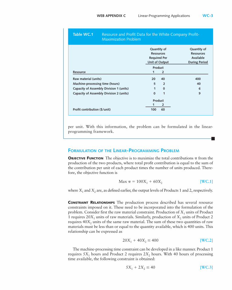
Consider the White Company, a manufacturer of gas (Product 1) and electric(Product 2) clothes dryers. The problem is to determine the optimal level of output(X1 and X2) for two products (1 and 2). Information about the problem is sum-marized in Table WC.1. Production consists of a machining process that takes rawmaterials and converts them into unassembled parts. These are then sent to one oftwo divisions for assembly into the final product—Division 1 for Product 1 andDivision 2 for Product 2.3 As listed in Table WC.1, Product 1 requires 20 units ofraw material and 5 hours of machine-processing time, whereas Product 2 requires40 units of raw material and 2 hours of machine-processing time. During theperiod, 400 units of raw material and 40 hours of machine-processing time areavailable. The capacities of the two assembly divisions during the period are 6 and9 units, respectively. The operating profit contribution per unit or, more accurately,the per-unit contribution to profit and overhead (fixed costs) is $100 for eachunit of Product 1 and $60 for each unit of Product 2. The contribution per unitrepresents the difference between the selling price per unit and the variable cost

3 This problem ignores any scheduling difficulties that may exist in the production process.

EXAMPLE

� MANAGERIAL CHALLENGEof shipping fuel. The airlift system also requires thatcargo handlers and ground crews be available to ser-vice the aircraft. Furthermore, schedulers must beable to deal with disruptions caused by bad weatherand emergency changes in shipping priorities.Adding just a couple of percentage points to the effi-ciency of the airlift system can save the Air Forcemillions of dollars annually in equipment, labor,

and fuel costs. Major commercial airlines, such asAmerican and United, face similar scheduling prob-lems. Complex resource-allocation problems suchas these can be solved using linear-programmingtechniques.

2 Based on articles in BusinessWeek (September 21, 1987), pp. 69–76; and (March 13, 1989), p. 77.


WEB APPENDIX C Linear-Programming Applications WC-3

per unit. With this information, the problem can be formulated in the linear-programming framework.

FORMULATION OF THE LINEAR-PROGRAMMING PROBLEM

OBJECTIVE FUNCTION The objective is to maximize the total contributions � from theproduction of the two products, where total profit contribution is equal to the sum ofthe contribution per unit of each product times the number of units produced. There-fore, the objective function is

Max � � 100X1 � 60X2 [WC.1]

where X1 and X2 are, as defined earlier, the output levels of Products 1 and 2, respectively.

CONSTRAINT RELATIONSHIPS The production process described has several resourceconstraints imposed on it. These need to be incorporated into the formulation of theproblem. Consider first the raw material constraint. Production of X1 units of Product1 requires 20X1 units of raw materials. Similarly, production of X2 units of Product 2requires 40X2 units of the same raw material. The sum of these two quantities of rawmaterials must be less than or equal to the quantity available, which is 400 units. Thisrelationship can be expressed as

20X1 � 40X2 � 400 [WC.2]

The machine-processing time constraint can be developed in a like manner. Product 1requires 5X1 hours and Product 2 requires 2X2 hours. With 40 hours of processingtime available, the following constraint is obtained:

5X1 � 2X2 � 40 [WC.3]

Quantity of Quantity of Resources Resources

Required Per Available Unit of Output During Period

ProductResource 1 2

Raw material (units) 20 40 400

Machine-processing time (hours) 5 2 40

Capacity of Assembly Division 1 (units) 1 0 6

Capacity of Assembly Division 2 (units) 0 1 9

Product1 2

Profit contribution ($/unit) 100 60

Table WC.1 Resource and Profit Data for the White Company Profit-Maximization Problem


The capacities of the two assembly divisions also limit output and consequentlyprofits. For Product 1, which must be assembled in Division 1, the constraint is

X1 � 6 [WC.4]

For Product 2, which must be assembled in Division 2, the constraint is

X2 � 9 [WC.5]

Finally, the logic of the production process suggests that negative output quantitiesare not possible. Therefore, each of the decision variables is constrained to benonnegative:

X1 � 0 X2 � 0 [WC.6]

Equations WC.1 through WC.6 constitute a linear-programming formulation of theprofit-maximization production problem.

ECONOMIC ASSUMPTIONS OF THE LINEAR-PROGRAMMING MODEL

In formulating this problem as a linear-programming model, one must understand theeconomic assumptions that are incorporated into the model. Basically, one assumesthat a series of linear (or approximately linear) relationships involving the decisionvariables exist over the range of alternatives being considered in the problem. For theresource inputs, one assumes that the prices of these resources to the firm are con-stant over the range of resource quantities under consideration. This assumption im-plies that the firm can buy as much or as little of these resources as it needs withoutaffecting the per unit cost.4 Such an assumption would rule out quantity discounts.One also assumes that there are constant returns to scale in the production process.In other words, in the production process, a doubling of the quantity of resourcesemployed doubles the quantity of output obtained, for any level of resources.5 Finally,one assumes that the market selling prices of the two products are constant over therange of possible output combinations.6 These assumptions are implied by the fixedper-unit profit contribution coefficients in the objective function. If the assumptionsare not valid, then the optimal solution to the linear-programming model will notnecessarily be an optimal solution to the actual decision-making problem. Althoughthese relationships need not be linear over the entire range of values of the decisionvariables, the linearity assumptions must be valid over the full range of values beingconsidered in the problem.


4 This assumption involves the concept of an atomistic buyer in a competitive factor or input market. SeeChapter 10 of the textbook for a discussion of this type of market.5 “Doubling the quantity of resources” is used as an example. More generally, one would say that a givenpercentage increase in each of the resources would result in an equivalent percentage increase in outputfor any given level of resources. See Chapter 7 of the textbook for a further discussion of the concept of returnsto scale.6 This assumption is satisfied in a perfectly competitive market for the two final products. Further discussion ofthis type of market is in Chapter 10 of the textbook.



GRAPHICAL SOLUTION OF THE LINEAR-PROGRAMMING PROBLEM

Various techniques are available for solving linear-programming problems. Forlarger problems involving more than two decision variables, one needs to employalgebraic methods to obtain a solution. Further discussion of these methods ispostponed until later in the appendix. For problems containing only two decisionvariables, graphical methods can be used to obtain an optimal solution. To under-stand the nature of the objective function and constraint relationships, it is helpfulto solve the preceding problem graphically. For this approach, graph the feasiblesolution space and objective function separately and then combine the two graphs toobtain the optimal solution.

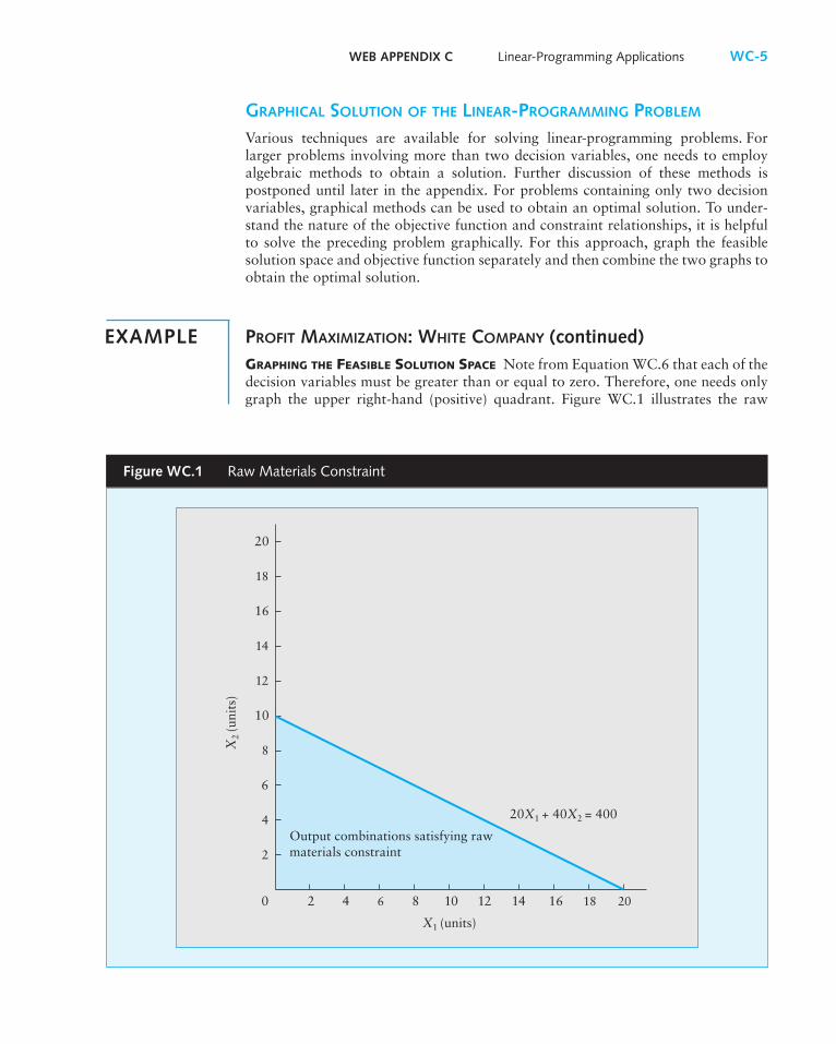
PROFIT MAXIMIZATION: WHITE COMPANY (continued)GRAPHING THE FEASIBLE SOLUTION SPACE Note from Equation WC.6 that each of thedecision variables must be greater than or equal to zero. Therefore, one needs onlygraph the upper right-hand (positive) quadrant. Figure WC.1 illustrates the raw

EXAMPLE

Figure WC.1 Raw Materials Constraint

0

X1 (units)

4

8

12

16

2 4 10 12 14 16

2

6

10

14

6 8 18 20

18

20

20X1 + 40X2 = 400

Output combinations satisfying rawmaterials constraint

X2

(uni

ts)



Feasible SolutionSpace

The set of all possiblecombinations of thedecision variables thatsimultaneously satis-fies all the constraintsof the problem.

material constraint as given by Equation WC.2. The upper limit or maximum quan-tity of raw materials that may be used occurs when the inequality is satisfied as anequality; in other words, the set of points that satisfies the equation

20X1 � 40X2 � 400

Because it is possible to use less than the amount of raw materials available, anycombination of outputs lying on or below this line (that is, the shaded area) willsatisfy the raw materials constraint.

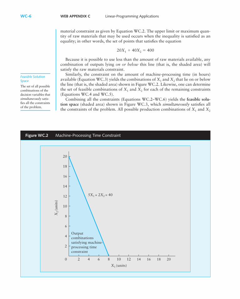
Similarly, the constraint on the amount of machine-processing time (in hours)available (Equation WC.3) yields the combinations of X1 and X2 that lie on or belowthe line (that is, the shaded area) shown in Figure WC.2. Likewise, one can determinethe set of feasible combinations of X1 and X2 for each of the remaining constraints(Equations WC.4 and WC.5).

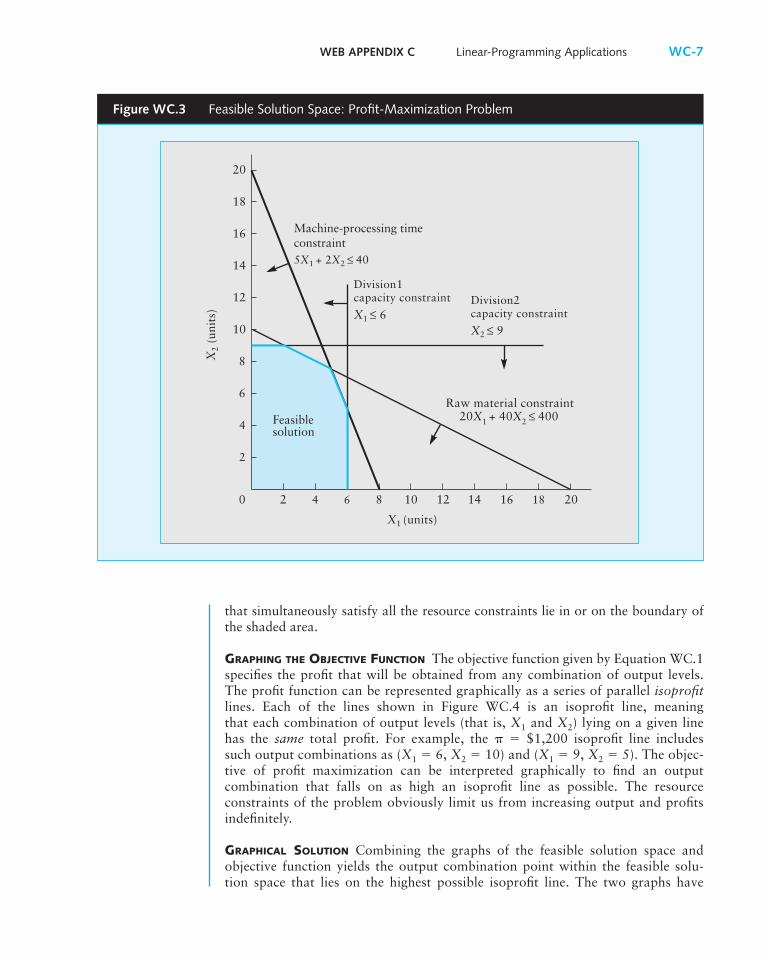
Combining all the constraints (Equations WC.2–WC.6) yields the feasible solu-tion space (shaded area) shown in Figure WC.3, which simultaneously satisfies allthe constraints of the problem. All possible production combinations of X1 and X2

Figure WC.2 Machine-Processing Time Constraint

0

X1 (units)

4

8

12

16

2 4 10 12 14 16

2

6

10

14

6 8 18 20

18

20

5X1 + 2X2 = 40

Outputcombinationssatisfying machine-processing timeconstraint

X2

(uni

ts)



Figure WC.3 Feasible Solution Space: Profit-Maximization Problem

0

X1 (units)

4

8

12

16

2 4 10 12 14 16

2

6

10

14

6 8 18 20

18

20

Feasible solution

Machine-processing timeconstraint 5X1 + 2X2 ≤ 40

Division1capacity constraint

X1 ≤ 6Division2capacity constraint

X2 ≤ 9

Raw material constraint20X1 + 40X2 ≤ 400

X2

(uni

ts)

that simultaneously satisfy all the resource constraints lie in or on the boundary ofthe shaded area.

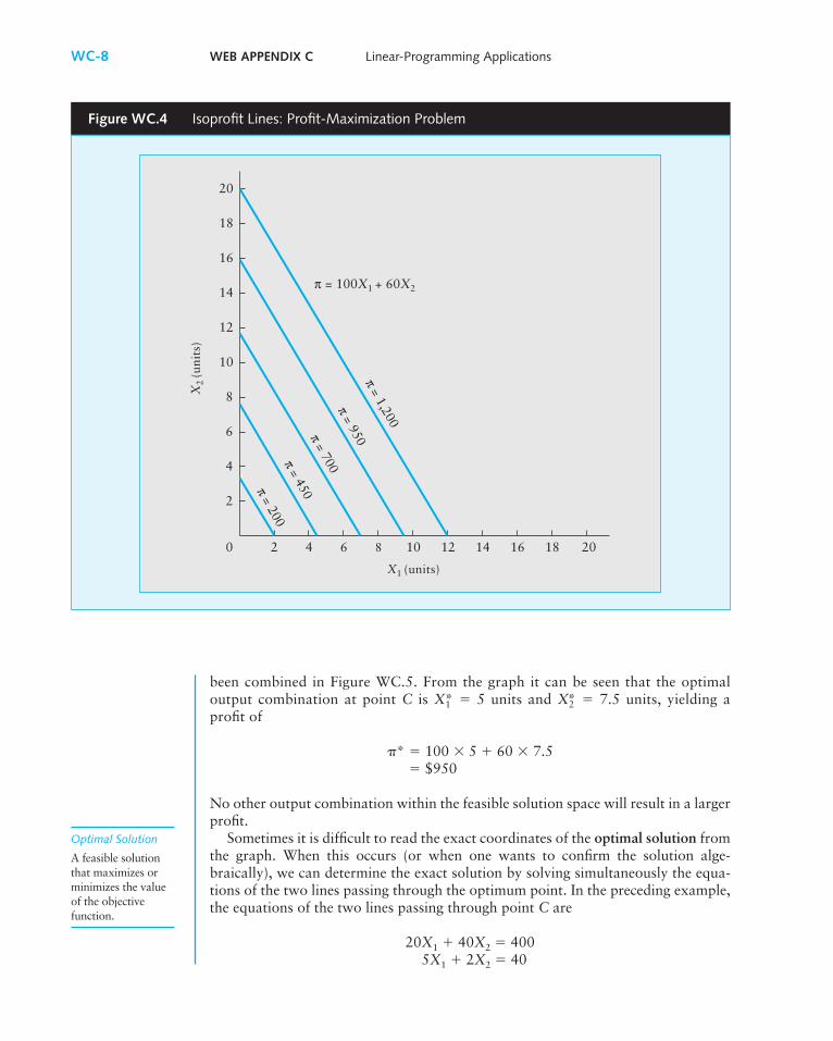
GRAPHING THE OBJECTIVE FUNCTION The objective function given by Equation WC.1specifies the profit that will be obtained from any combination of output levels.The profit function can be represented graphically as a series of parallel isoprofitlines. Each of the lines shown in Figure WC.4 is an isoprofit line, meaningthat each combination of output levels (that is, X1 and X2) lying on a given linehas the same total profit. For example, the � � $1,200 isoprofit line includessuch output combinations as (X1 � 6, X2 � 10) and (X1 � 9, X2 � 5). The objec-tive of profit maximization can be interpreted graphically to find an outputcombination that falls on as high an isoprofit line as possible. The resourceconstraints of the problem obviously limit us from increasing output and profitsindefinitely.

GRAPHICAL SOLUTION Combining the graphs of the feasible solution space andobjective function yields the output combination point within the feasible solu-tion space that lies on the highest possible isoprofit line. The two graphs have


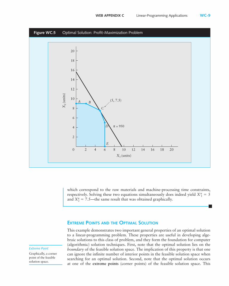
been combined in Figure WC.5. From the graph it can be seen that the optimaloutput combination at point C is X1* � 5 units and X2* � 7.5 units, yielding aprofit of

�* � 100 � 5 � 60 � 7.5� $950

No other output combination within the feasible solution space will result in a largerprofit.

Sometimes it is difficult to read the exact coordinates of the optimal solution fromthe graph. When this occurs (or when one wants to confirm the solution alge-braically), we can determine the exact solution by solving simultaneously the equa-tions of the two lines passing through the optimum point. In the preceding example,the equations of the two lines passing through point C are

20X1 � 40X2 � 4005X1 � 2X2 � 40


Optimal Solution

A feasible solutionthat maximizes orminimizes the valueof the objectivefunction.

Figure WC.4 Isoprofit Lines: Profit-Maximization Problem

0

X1 (units)

4

8

12

16

2 4 10 12 14 16

2

6

10

14

6 8 18 20

18

20

π = 100X1 + 60X2

π = 1,200

π = 950π = 700π = 450π = 200

X2

(uni

ts)



Figure WC.5 Optimal Solution: Profit-Maximization Problem

0

X1 (units)

4

8

12

16

2 4 10 12 14 16

2

6

10

14

201886

18

20

E

D

C

BA (5, 7.5)

π = 950

X2

(uni

ts)

which correspond to the raw materials and machine-processing time constraints,respectively. Solving these two equations simultaneously does indeed yield X*1 � 5and X*2 � 7.5—the same result that was obtained graphically.

EXTREME POINTS AND THE OPTIMAL SOLUTION

This example demonstrates two important general properties of an optimal solutionto a linear-programming problem. These properties are useful in developing alge-braic solutions to this class of problem, and they form the foundation for computer(algorithmic) solution techniques. First, note that the optimal solution lies on theboundary of the feasible solution space. The implication of this property is that onecan ignore the infinite number of interior points in the feasible solution space whensearching for an optimal solution. Second, note that the optimal solution occursat one of the extreme points (corner points) of the feasible solution space. This

Extreme Point

Graphically, a cornerpoint of the feasiblesolution space.


property reduces even further the magnitude of the search procedure for an optimalsolution. For this example it means that from among the infinite number of pointslying on the boundary of the feasible solution space, only six points—A, B, C, D, E,and zero—need to be examined to find an optimal solution.

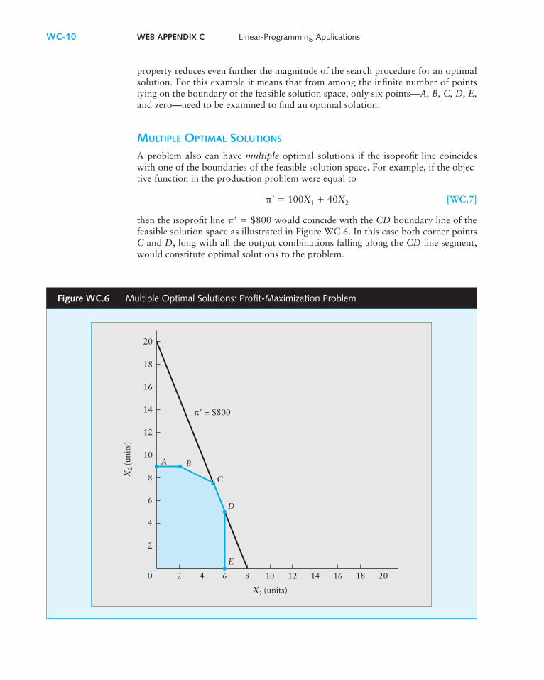
MULTIPLE OPTIMAL SOLUTIONS

A problem also can have multiple optimal solutions if the isoprofit line coincideswith one of the boundaries of the feasible solution space. For example, if the objec-tive function in the production problem were equal to

�� 100X1 � 40X2 [WC.7]

then the isoprofit line �� $800 would coincide with the CD boundary line of thefeasible solution space as illustrated in Figure WC.6. In this case both corner pointsC and D, long with all the output combinations falling along the CD line segment,would constitute optimal solutions to the problem.


Figure WC.6 Multiple Optimal Solutions: Profit-Maximization Problem

0

X1 (units)

4

8

12

16

2 4 10 12 14 16

2

6

10

14

6 20188

18

20

E

D

C

BA

π = $800

X2

(uni

ts)


SLACK VARIABLES

In addition to the optimal combination of output to produce (X*1 and X*2) and themaximum total profit (�*), we are also interested in the amount of each resourceused in the production process. For the production of 5 units (�X*1) and 7.5 units(�X*2 ) of products 1 and 2, respectively, the resource requirements (from EquationsWC.2–WC.5) are as follows:

20(5) � 40(7.5) � 400 units of raw materials5(5) � 2(7.5) � 40 hours of machine-processing time

1(5) � 5 units of Division 1 assembly capacity1(7.5) � 7.5 units of Division 2 assembly capacity

This information indicates that all available raw materials (400 units) and allavailable machine-processing time (40 hours) will be used in producing the optimaloutput combination. However, 1 unit of Division 1 assembly capacity (6 – 5) and1.5 units of Division 2 assembly capacity (9 – 7.5) will be unused in producing theoptimal output combination. These unused or idle resources associated with a lessthan or equal to constraint (�) are referred to as slack.

Slack variables can be added to the formulation of a linear-programmingproblem to represent this slack or idle capacity. Slack variables are given a coef-ficient of zero in the objective function because they make no contributionto profit. Slack variables can be thought of as representing the difference betweenthe right-hand side and left-hand side of a less than or equal to inequality (�)constraint.

In the preceding profit-maximization problem (Equations WC.1–WC.6), fourslack variables (S1, S2, S3, S4) are used to convert the four (less than or equal to) con-straints to equalities as follows:

Max � � 100X1 � 60X2 � 0S1 � 0S2 � 0S3 � 0S4

20X1 � 40X2 � 1S1 � 4005X1 � 2X2 � 1S2 � 40X1 � 1S3 � 6

X2 � 1S4 � 9X1, X2, S1, S2, S3, S4 � 0

As shown later in the appendix, a computer solution of a linear-programmingproblem automatically provides the optimal values of the slack variables along withthe optimal values for the original decision variables.

THE DUAL PROBLEM AND INTERPRETATIONOF THE DUAL VARIABLES

The solution of a linear-programming problem, in addition to providing the opti-mal values of the decision variables, contains information that can be very usefulin making marginal resource-allocation decisions. This marginal information iscontained in what are known as the dual variables of the linear-programmingproblem.


Slack Variable

A variable that representsthe difference betweenthe right-hand side andleft-hand side of a lessthan or equal to (�)inequality constraint. Itis added to the left-handside of the inequality toconvert the constraint toan equality. It measuresthe amount of an unusedor idle resource.

Dual Variable

A variable that mea-sures how much theobjective function(e.g., profit or cost) willchange if a given con-straint is increased byone unit, provided theincrease in the resourcedoes not shift the opti-mal solution to anotherextreme point of thefeasible solution space.


THE DUAL LINEAR-PROGRAMMING PROBLEM

Associated with every linear-programming problem is a related dual linear-programming problem. The originally formulated problem, in relation to the dualproblem, is known as the primal linear-programming problem.7 If the objective inthe primal problem is maximization of some function, then the objective in the dualproblem is minimization of a related (but different) function. Conversely, a primalminimization problem has a related dual maximization problem. The dual variablesrepresent the variables contained in the dual problem.

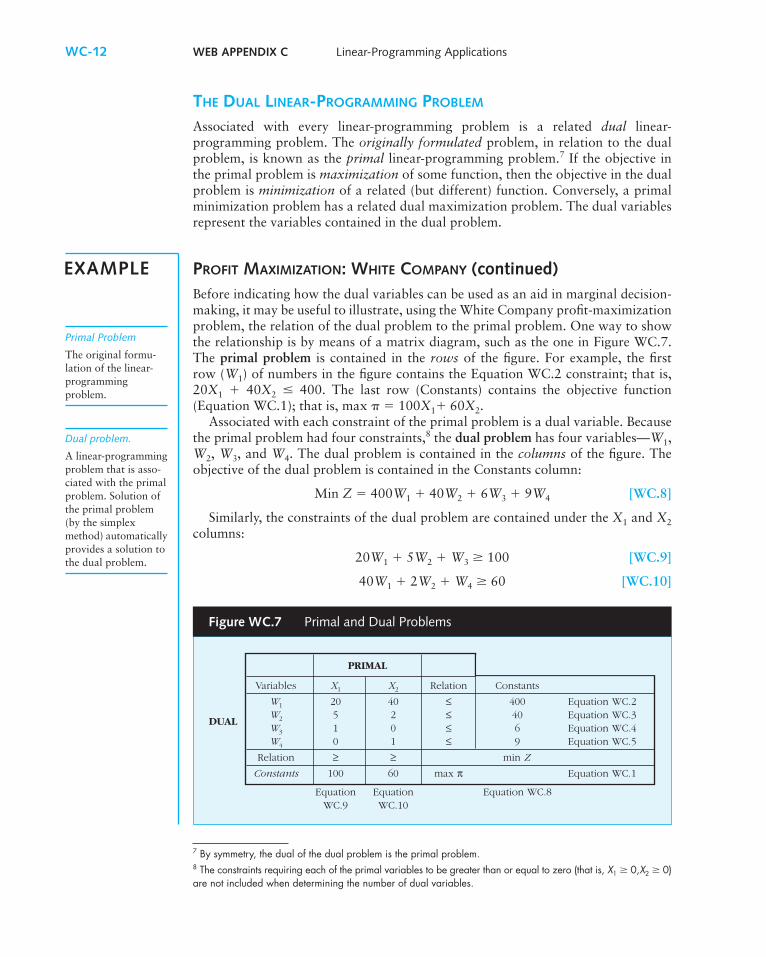
PROFIT MAXIMIZATION: WHITE COMPANY (continued)Before indicating how the dual variables can be used as an aid in marginal decision-making, it may be useful to illustrate, using the White Company profit-maximizationproblem, the relation of the dual problem to the primal problem. One way to showthe relationship is by means of a matrix diagram, such as the one in Figure WC.7.The primal problem is contained in the rows of the figure. For example, the firstrow (W1) of numbers in the figure contains the Equation WC.2 constraint; that is,20X1 � 40X2 � 400. The last row (Constants) contains the objective function(Equation WC.1); that is, max � � 100X1� 60X2.

Associated with each constraint of the primal problem is a dual variable. Becausethe primal problem had four constraints,8 the dual problem has four variables—W1,W2, W3, and W4. The dual problem is contained in the columns of the figure. Theobjective of the dual problem is contained in the Constants column:

Min Z � 400W1 � 40W2 � 6W3 � 9W4 [WC.8]

Similarly, the constraints of the dual problem are contained under the X1 and X2columns:

20W1 � 5W2 � W3 � 100 [WC.9]

40W1 � 2W2 � W4 � 60 [WC.10]


7 By symmetry, the dual of the dual problem is the primal problem.8 The constraints requiring each of the primal variables to be greater than or equal to zero (that is, X1 � 0,X2 � 0)are not included when determining the number of dual variables.

Primal Problem

The original formu-lation of the linear-programmingproblem.

Dual problem.

A linear-programmingproblem that is asso-ciated with the primalproblem. Solution ofthe primal problem(by the simplexmethod) automaticallyprovides a solution tothe dual problem.

EXAMPLE

Figure WC.7 Primal and Dual Problems

PRIMAL

Variables X1 X2 Relation Constants

W1 20 40 ≤ 400 Equation WC.2

DUALW2 5 2 ≤ 40 Equation WC.3W3 1 0 ≤ 6 Equation WC.4W4 0 1 ≤ 9 Equation WC.5

Relation ≥ ≥ min Z

Constants 100 60 max π Equation WC.1

Equation Equation Equation WC.8WC.9 WC.10


One also requires

W1 � 0, W2 � 0, W3 � 0, W4 � 0 [WC.11]

In general, a primal problem with n variables and m constraints will have as its duala problem with m variables and n constraints.

ECONOMIC INTERPRETATION OF THE DUAL VARIABLES

In the preceding resource-constrained profit-maximization problem, a dual variableexisted for each of the limited resources required in the production process. In sucha problem the dual variables measure the “imputed values” or shadow prices of eachof the scarce resources. Expressed in dollars per unit of resource, they give anindication of how much each resource contributes to the overall profit function. Withthis interpretation of the dual variables, the dual objective function (Equation WC.8)is to minimize the total cost or value of the resources employed in the process. The twodual constraints (Equations WC.9 and WC.10) require that the value of the resourcesused in producing one unit each of X1 and X2 be at least as great as the profit re-ceived from the sale of one unit of each product. An important linear-programmingtheorem, known as the duality theorem, indicates that the maximum value of theprimal profit function will also be equal to the minimum value of the dual “imputedvalue” function.9 The solution of the dual problem in effect apportions the totalprofit figure among the various scarce resources employed in the process.

The interpretation of the dual variables and dual problem depends on the natureand objective of the primal problem. Thus a completely different interpretation isinvolved whenever the primal problem is one of cost minimization.10

PROFIT MAXIMIZATION: WHITE COMPANY (continued)The preceding example illustrates how the dual variables can be used to makemarginal resource-allocation decisions. The values of the dual variables, which areobtained automatically in an algebraic solution of the linear-programming problem,are W1* � $0.625per unit, W2* � $17.50 per unit, W3* � $0 per unit, W4* � $0 perunit. Each dual variable indicates the rate of change in total profits for an incremen-tal change in the amount of each of the various resources. In this way they are simi-lar to the values used in the Lagrangian multiplier technique. The dual variablesindicate how much the total profit will change (i.e., marginal profit) if one additionalunit of a given resource is made available, provided the increase in the resource doesnot shift the optimal solution to another corner point of the feasible solution space.For example, W2* � $17.50 indicates that profits could be increased by as much as$17.50 if an additional unit (hour) of machine capacity could be made available to


9 See any standard linear-programming text, such as the previously cited Anderson et al., and George B.Dantzig, Linear Programming and Extensions (Princeton, NJ: Princeton University Press, 1963); see G. Hadley,Linear Programming (Reading, MA: Addison-Wesley, 1962), for a complete discussion of the concept of dualityand the duality theorem.10 See Hadley, Linear Programming, pp. 485–487; and J. G. Kemeny, H. Mirkil, J. L. Snell, and G. L. Thompson,Finite Mathematical Structures (Englewood Cliffs, NJ: Prentice Hall, 1959), pp. 364–366, and the next section,for examples of the interpretation of other types of dual problems.

Shadow Price

Measures the value (thatis, contribution to theobjective function) ofone additional unit of aresource. It is equivalentto the dual variable.

EXAMPLE


the production process. This type of information is potentially useful in making de-cisions about purchasing or renting additional machine capacity or using existingmachine capacity more fully through the use of overtime and multiple shifts. A dualvariable equal to zero, such as W*3 and W*4, indicates that profits would not increaseif additional resources of these types were made available; in fact, excess capacity inthese resources exists. (Recall in the discussion of slack variables, portions of theseresources were unused or idle in the optimal solution.) This discussion only indicatesthe type of analysis that is possible. Much more detailed analysis of this nature canbe performed using parametric-programming techniques.11

A COST-MINIMIZATION PROBLEM

This section develops a cost-minimization problem and illustrates the use of com-puter programs for its solution.

STATEMENT OF THE PROBLEM

Large multiplant firms often produce the same products at two or more factories.Often these factories employ different production technologies and have differentunit production costs. The objective is to produce the desired amount of outputusing the given facilities (that is, plants and production processes) to minimize pro-duction costs.

COST MINIMIZATION: SILVERADO MINING COMPANY

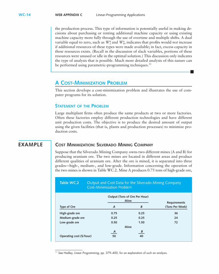
Suppose that the Silverado Mining Company owns two different mines (A and B) forproducing uranium ore. The two mines are located in different areas and producedifferent qualities of uranium ore. After the ore is mined, it is separated into threegrades—high-, medium-, and low-grade. Information concerning the operation ofthe two mines is shown in Table WC.2. Mine A produces 0.75 tons of high-grade ore,


11 See Hadley, Linear Programming, pp. 379–400, for an explanation of such an analysis.

EXAMPLE

Output (Tons of Ore Per Hour) Mine

Requirements Type of Ore A B (Tons Per Week)

High-grade ore 0.75 0.25 36

Medium-grade ore 0.25 0.25 24

Low-grade ore 0.50 1.50 72

Mine

A B

Operating cost ($/hour) 50 40

Table WC.2 Output and Cost Data for the Silverado Mining Company Cost-Minimization Problem


0.25 tons of medium-grade ore, and 0.50 tons of low-grade ore per hour. Likewise,Mine B produces 0.25, 0.25, and 1.50 tons of high-, medium-, and low-grade ore perhour, respectively. The firm has contracts with uranium-processing plants to supplya minimum of 36 tons of high-grade ore, 24 tons of medium-grade ore, and 72 tonsof low-grade ore per week. These figures are shown in the Requirements column ofTable WC.2. Finally, as shown in the bottom row of Table WC.2, it costs the com-pany $50 per hour to operate Mine A and $40 per hour to operate Mine B. The com-pany wishes to determine the number of hours per week it should operate each mineto minimize the total cost of fulfilling its supply contracts.

FORMULATION OF THE LINEAR-PROGRAMMING PROBLEM

OBJECTIVE FUNCTION The objective is to minimize the total cost per week (C) fromthe operation of the two mines, where the total cost is equal to the sum of the oper-ating cost per hour of each mine times the number of hours per week that each mine isoperated. Defining X1 as the number of hours per week that Mine A is operated andX2 as the number of hours per week that Mine B is operated, the objective function is

Min C � 50X1 � 40X2 [WC.12]

CONSTRAINT RELATIONSHIPS The Silverado Mining Company’s contracts with uranium-processing plants require it to operate the two mines for a sufficient number of hoursto produce the required amount of each grade of uranium ore. In the production ofhigh-grade ore, Mine A produces 0.75 tons per hour times the number of hours perweek (X1) that it operates, and Mine B produces 0.25 tons per hour times the numberof hours per week (X2) that it operates. The sum of these two quantities must begreater than or equal to the required output of 36 tons per week. This relationshipcan be expressed as

0.75X1 � 0.25X2 � 36 [WC.13]

Similar constraints can be developed for the production of medium-grade ore

0.25X1 � 0.25X2 � 24 [WC.14]

and low-grade ore

0.50X1 � 1.50X2 � 72 [WC.15]

Finally, negative production times are not possible. Therefore, each of the deci-sion variables is constrained to be nonnegative:

X1 � 0, X2 � 0 [WC.16]

Equations WC.12 through WC.16 represent a linear-programming formulationof the cost-minimization production problem.

SLACK (SURPLUS) VARIABLES

Recall from the discussion of the maximization problem earlier in the appendix thatslack variables were added to the less than or equal to inequality (�) constraints toconvert these constraints to equalities. Similarly, in a minimization problem, surplusvariables are subtracted from the greater than or equal to inequality (�) constraints


Surplus Variables

A variable that repre-sents the differencebetween the right-handside and left-hand side ofa greater than or equalto (�) inequality con-straint. It is subtractedfrom the left-hand sideof the inequality to con-vert the constraint toan equality. It measuresthe amount of a prod-uct (or output) in excessof the required amount.


to convert these constraints to equalities. Like the slack variables, surplus variablesare given coefficients of zero in the objective function because they have no effect onthe value.

COST MINIMIZATION: SILVERADO MINING COMPANY (continued)In the preceding cost-minimization problem, three surplus variables (S1, S2, S3)are used to convert the three (greater than or equal to) constraints to equalitiesas follows:

Min C � 50X1 � 40X2 � 0S1 � 0S2 � 0S3s.t. 0.75X1 � 0.25X2 1S1 � 36

0.25X1 � 0.25X2 1S2 � 240.50X1 � 1.50X2 1S3 � 72

X1, X2, S1, S2, S3 � 0

COMPUTER SOLUTION OF THE LINEAR-PROGRAMMING PROBLEM

The solution of large-scale linear-programming problems typically employs a proce-dure (or variation of the procedure) known as the simplex method. Basically, the sim-plex method is a step-by-step procedure for moving from corner point to corner pointof the feasible solution space in such a manner that successively larger (or smaller)values of the maximization (or minimization) objective function are obtained at eachstep. The procedure is guaranteed to yield the optimal solution in a finite number ofsteps. Further discussion of this method is beyond the scope of this appendix.12

Most practical applications of linear programming use computer programs toperform the calculations and obtain the optimal solution. Although many differentprograms are available for solving linear-programming problems, the output of theseprograms usually includes the optimal solution to the primal problem as well as theoptimal values of the dual variables. The particular program illustrated here isknown as SIMPLX.13 (Similar programs are likely to be readily available on yourpersonal computer or school’s computer system.)

COST MINIMIZATION: SILVERADO MINING COMPANY (continued)Putting the objective function and constraints (Equations WC.12 through WC.16)along with the appropriate control statements into the SIMPLX program yields theoutput shown in Figure WC.8. The optimal values of the decision variables are shownin the Primal Solution column—X*1 � 24 and X*2 � 72. The firm should operateMine A for 24 hours per week and Mine B for 72 hours per week to minimize totaloperating costs, which yields a minimum total cost of $4,080 per week.

Note also that the optimal value of the surplus variable S*3 [that is, X(5) on thecomputer output] is 48, to indicate that a surplus of 48 tons of low-grade ore (that


Simplex Method

A step-by-step mathe-matical procedure forfinding the optimalsolution to a linear-programming problem.

EXAMPLE

EXAMPLE

12 Any basic linear-programming textbook, such as the previously cited Anderson et al., Dantzig, and Hadleybooks, contains detailed discussions of this procedure.13 “SIMPLX” is a terminal-oriented computer program. See E. Pearsall and B. Price, Linear Programming andSimulation (No. MS(350)), CONDUIT (Ames: Iowa State University).


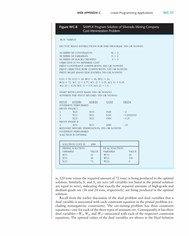
is, 120 tons versus the required amount of 72 tons) is being produced in the optimalsolution. Similarly, S1 and S2 are zero (all variables not listed in the primal solutionare equal to zero), indicating that exactly the required amounts of high-grade andmedium-grade ore (36 and 24 tons, respectively) are being produced in the optimalsolution.

Recall from the earlier discussion of the dual problem and dual variables that adual variable is associated with each constraint equation in the primal problem (ex-cluding nonnegativity constraints). The ore-mining problem has three constraintequations—one for each of the three types of uranium ore. Consequently, it has threedual variables—W1, W2, and W3—associated with each of the respective constraintequations. The optimal values of the dual variables are shown in the Dual Solution


Figure WC.8 SIMPLX Program Solution of Silverado Mining Company Cost-Minimization Problem

:RUN “SIMPLX”

DO YOU WANT INSTRUCTIONS FOR THIS PROGRAM: YES OR NO?$NO

NUMBER OF CONSTRAINTS: M � 3NUMBER OF VARIABLES: N � 2NUMBER OF SLACKS CREATED: S � 3OBJECTIVE IS TO MINIMIZE COSTPRINT CONSTRAINT COEFFICIENTS: YES OR NO?$YESPRINT OBJECTIVE ROW COEFFICIENTS: YES OR NO?$YESPRINT RIGHT HAND SIDE ENTRIES: YES OR NO?$YES

C(1) � 50, C(2) � 40, B(1) � 36, B(2) � 24.B(3) � 72, A(1, 1) � 0.75, A(1, 2) � 0.25, A(2, 1) � 0.25,A(2, 2) � 0.25, A(3, 1) � 0.5, A(3, 2) � 1.5,

START WITH GIVEN BASIS: YES OR NO?$NOSUPPRESS THE PIVOT RECORD: YES OR NO?$NO

PIVOT ENTERS LEAVES COST DELTAINVERSION PERFORMEDBEGIN PHASE I1 X(2) X(0) 1920 22 X(1) X(0) 3240 0.83333333 X(3) X(0) 4560 0.25BEGIN PHASE II4 X(5) X(3) 4080 10REINVERT BEFORE TERMINATION: YES OR NO?$YESINVERSION PERFORMEDSOLUTION IS OPTIMAL

SOLUTION COST IS 4080

PRIMAL SOLUTION DUAL SOLUTIONVARIABLE VALUE VARIABLE VALUEX(1) 24 W(1) 20X(5) 48 W(2) 140X(2) 72 W(3) 0


column of Figure WC.8—W*1 � $20, W*2 � $140, and W*3 � $0. Each dual variablemeasures the change in total cost (i.e., marginal cost) that results from a one-unit(ton) increase in the required output, provided that the increase does not shift the op-timal solution to another corner point of the feasible solution space. For example,W*1 � $20 indicates that total costs will increase by as much as $20 if the firm isrequired to produce an additional ton of high-grade uranium ore. Comparison ofthis value to the revenue received per ton of ore can help the firm in making decisionsabout whether to expand or contract its mining operations.

Next, consider the interpretation of W*3 � $0. This zero value indicates thatsurplus low-grade ore is being produced by the firm. (Recall that S*3 � 48.) At theoptimal solution (operating Mines A and B at 24 and 72 hours per week, respec-tively), the cost of producing an additional ton of low-grade ore is $0.

A NEW TECHNIQUE FOR SOLVING LARGE-SCALELINEAR-PROGRAMMING PROBLEMS

Since its development in 1947 by operations research pioneer George Dantzig, mostlinear-programming problems have been solved using the simplex method (or varia-tions thereof). Approximately 80 to 90 percent of these constrained optimizationproblems can be solved on computers using this algorithm. However, when solvingextremely large problems or problems that are changing rapidly, the simplex methodoften is too slow to be practical.

An AT&T Bell Laboratories researcher, Narendra Karmarkar, developed analternative solution technique that is potentially 50 to 100 times faster than the sim-plex method in solving large, complex linear-programming problems. For example,Bell Laboratories (now Lucent Technologies) is using Karmarkar’s algorithm to fore-cast the most cost-effective way to satisfy the future needs over a 10-year horizon ofthe telephone network linking 20 countries on the rim of the Pacific Ocean. Theresulting linear-programming problem contains 42,000 variables. Solving this prob-lem using the simplex method would require 4 to 7 hours of mainframe computertime to answer each “what-if” question, whereas this new technique would requireless than 4 minutes.

In another application, Karmarkar’s algorithm was used to solve the MilitaryAirlift Command’s scheduling problem described in the Managerial Challenge sectionat the beginning of the appendix. Solving this linear-programming problem, whichinvolves 321,000 variables and 14,000 constraints, required only one hour of com-puter time—just a fraction of the time that would be required using the simplexmethod. Given the new method’s ability to solve large problems quickly, the MilitaryAirlift Command, as well as commercial airlines such as American and United,should be able to solve complex scheduling problems and make efficient adjustmentsrapidly in response to changing operating constraints.

ADDITIONAL LINEAR-PROGRAMMING EXAMPLES

Linear programming is useful in a wide variety of managerial resource-allocationproblems. This section examines some additional applications in finance, marketing,and distribution.



THE CAPITAL-RATIONING PROBLEM: ASPEN SKI COMPANY

Rather than letting the size of their capital budgets (expenditures that areexpected to provide long-term benefits to the firm, such as plants and equipment)be determined by the number of profitable investment opportunities available(all investment projects meeting some acceptance standard), many firms placean upper limit or constraint on the amount of funds allocated to capital invest-ment. Capital rationing takes place whenever the total cash outlays for all pro-jects that meet some acceptance standard exceed the constraint on total capitalinvestment.

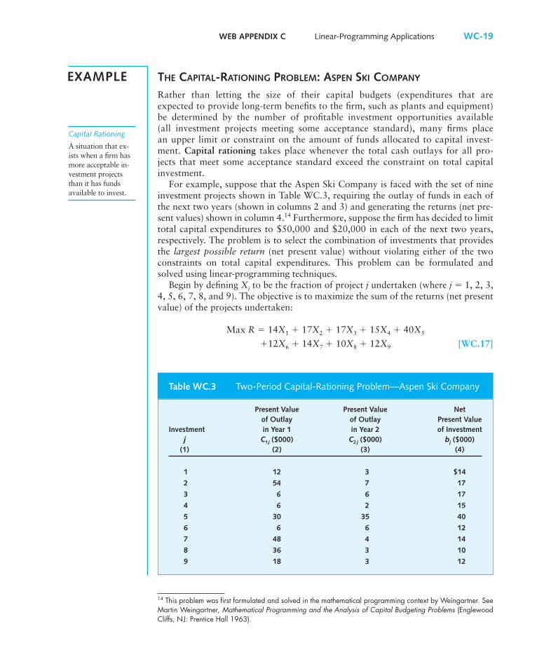
For example, suppose that the Aspen Ski Company is faced with the set of nineinvestment projects shown in Table WC.3, requiring the outlay of funds in each ofthe next two years (shown in columns 2 and 3) and generating the returns (net pre-sent values) shown in column 4.14 Furthermore, suppose the firm has decided to limittotal capital expenditures to $50,000 and $20,000 in each of the next two years,respectively. The problem is to select the combination of investments that providesthe largest possible return (net present value) without violating either of the twoconstraints on total capital expenditures. This problem can be formulated andsolved using linear-programming techniques.

Begin by defining Xj to be the fraction of project j undertaken (where j � 1, 2, 3,4, 5, 6, 7, 8, and 9). The objective is to maximize the sum of the returns (net presentvalue) of the projects undertaken:

Max R � 14X1 � 17X2 � 17X3 � 15X4 � 40X5

�12X6 � 14X7 � 10X8 � 12X9 [WC.17]


EXAMPLE

Capital Rationing

A situation that ex-ists when a firm hasmore acceptable in-vestment projectsthan it has fundsavailable to invest.

Present Value Present Value Netof Outlay of Outlay Present Value

Investment in Year 1 in Year 2 of Investmentj C1j ($000) C2 j ($000) bj ($000)

(1) (2) (3) (4)

1 12 3 $14

2 54 7 17

3 6 6 17

4 6 2 15

5 30 35 40

6 6 6 12

7 48 4 14

8 36 3 10

9 18 3 12

Table WC.3 Two-Period Capital-Rationing Problem—Aspen Ski Company

14 This problem was first formulated and solved in the mathematical programming context by Weingartner. SeeMartin Weingartner, Mathematical Programming and the Analysis of Capital Budgeting Problems (EnglewoodCliffs, NJ: Prentice Hall 1963).


The constraints are the restrictions placed on total capital expenditures in each ofthe two years:

12X1 � 54X2 � 6X3 � 6X4 � 30X5 � 6X6 � 48X7

� 36X8 � 18X9 � 50 [WC.18]

3X1 � 7X2 � 6X3 � 2X4 � 35X5 � 6X6 � 4X7

� 3X8 � 3X9 � 20 [WC.19]

Also, so that no more than one of any project will be included in the final solu-tion, all the Xj’s must be less than or equal to 1:

X1 � 1 [WC.20]

X2 � 1 [WC.21]

X3 � 1 [WC.22]

X4 � 1 [WC.23]

X5 � 1 [WC.24]

X6 � 1 [WC.25]

X7 � 1 [WC.26]

X8 � 1 [WC.27]

X9 � 1 [WC.28]

Finally, all the Xj’s must be nonnegative:

X1 � 0, X2 � 0, X3 � 0, X4 � 0, X5 � 0, X6 � 0, X7 � 0, X8 � 0, X9 � 0 [WC.29]

Equations WC.17–WC.29 represent a linear-programming formulation of thiscapital-rationing problem.

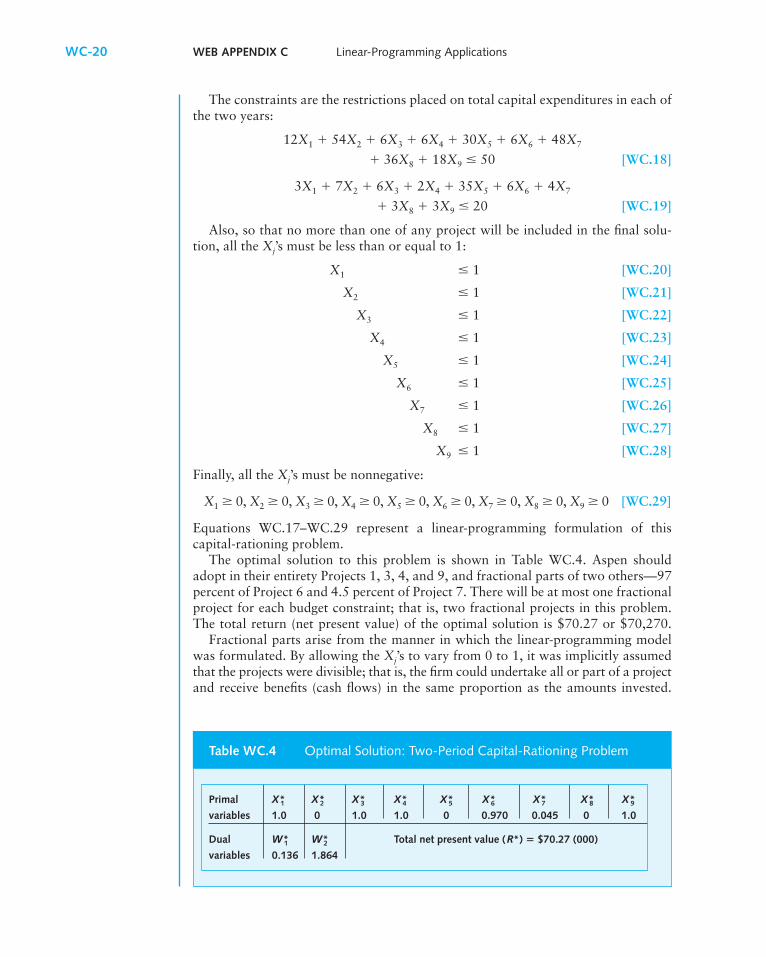
The optimal solution to this problem is shown in Table WC.4. Aspen shouldadopt in their entirety Projects 1, 3, 4, and 9, and fractional parts of two others—97percent of Project 6 and 4.5 percent of Project 7. There will be at most one fractionalproject for each budget constraint; that is, two fractional projects in this problem.The total return (net present value) of the optimal solution is $70.27 or $70,270.

Fractional parts arise from the manner in which the linear-programming modelwas formulated. By allowing the Xj’s to vary from 0 to 1, it was implicitly assumedthat the projects were divisible; that is, the firm could undertake all or part of a projectand receive benefits (cash flows) in the same proportion as the amounts invested.


Primal X*1 X*2 X*3 X*4 X*5 X*6 X*7 X*8 X*9variables 1.0 0 1.0 1.0 0 0.970 0.045 0 1.0

Dual W*1 W*2 Total net present value (R*) � $70.27 (000)

variables 0.136 1.864

Table WC.4 Optimal Solution: Two-Period Capital-Rationing Problem


This assumption is somewhat unrealistic because most investments must either beundertaken in their entirety or not at all. One possible way to eliminate these fractionalprojects is to adjust the budget constraints upward to be able to include the entireproject. Generally, total capital expenditure limits are flexible enough to allow slightupward adjustments to be made. Another method for eliminating fractional pro-jects in the solution is to use an integer-programming formation of the problem.This would be done by adding constraints to the model that require the Xj’s to haveinteger values:

Xj an integer j � 1, . . . , 9

that is X1, X2, X3, X4, X5, X6, X7, X8, X9 are integers. Requiring the Xj’s to be inte-gers and also to be between 0 and 1 forces these variables to take on the values ofeither 1 or 0; that is, the projects would have to be accepted either in their entiretyor not at all.

The solution to this primal linear-programming problem also yields a solution tothe dual problem. There is one dual variable for every constraint in the primal problem.The optimal values of the dual variables associated with the two budget constraints(Equations WC.18 and WC.19) are shown in Table WC.4. In this problem thesedual variables indicate the amount that the total present value could be increased ifthe budget limits (constraints) were increased to permit an additional $1 investmentin the given period. In the example, if the budget constraint in Year 1 were increasedfrom $50,000 to $51,000, then the total net present value would increase by W*1 �$0.136 � 1,000 or $136. Similarly, if the budget constraint in Year 2 were increasedfrom $20,000 to $21,000, the total net present value would increase by W*2 �$1.864 � 1,000 or $1,864. Because the dual variables measure the opportunity costof not having additional funds available for investment in a given period, they canbe used in deciding whether or not to shift funds from one period to another.15 If thevalues of the dual variables are fairly large, indicating that total net present valuecould be increased significantly through additional investment, the firm may decide toincrease its capital expenditure budget through such methods as new borrowing orequity financing.

THE TRANSPORTATION PROBLEM: MERCURY CANDY COMPANY

Large multiplant firms often produce their products at several different factories andthen ship the products to various regional warehouses located throughout their mar-keting area. The objective is to minimize shipping costs subject to the constraints ofmeeting the demand for the product in each region and not exceeding the supply ofthe product available at each plant.


EXAMPLE

15 The formulation of the capital-rationing problem in a linear-programming framework creates a difficulty ininterpreting the dual variables associated with budget constraints. A problem arises because two interdependentmeasures of the opportunity cost of investment funds are available—the dual variable value and the cost ofcapital (discount rate), which is used in finding the net present values (bj’s) of the investment projects. For afurther discussion of the problem, see William J. Baumol and Richard E. Quandt, “Investment and Discount RatesUnder Capital Rationing—A Programming Approach,” Economic Journal 75 (June 1965), pp. 317–329.


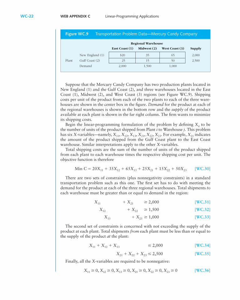
Suppose that the Mercury Candy Company has two production plants located inNew England (1) and the Gulf Coast (2), and three warehouses located in the EastCoast (1), Midwest (2), and West Coast (3) regions (see Figure WC.9). Shippingcosts per unit of the product from each of the two plants to each of the three ware-houses are shown in the center box in the figure. Demand for the product at each ofthe regional warehouses is shown in the bottom row and the supply of the productavailable at each plant is shown in the far right column. The firm wants to minimizeits shipping costs.

Begin the linear-programming formulation of the problem by defining Xij to bethe number of units of the product shipped from Plant i to Warehouse j. This problemhas six X-variables—namely, X11, X12, X13, X21, X22, X23. For example, X21 indicatesthe amount of the product shipped from the Gulf Coast plant to the East Coastwarehouse. Similar interpretations apply to the other X-variables.

Total shipping costs are the sum of the number of units of the product shippedfrom each plant to each warehouse times the respective shipping cost per unit. Theobjective function is therefore

Min C � 20X11 � 35X12 � 65X13 � 25X21 � 15X22 � 50X23 [WC.30]

There are two sets of constraints (plus nonnegativity constraints) in a standardtransportation problem such as this one. The first set has to do with meeting thedemand for the product at each of the three regional warehouses. Total shipments toeach warehouse must be greater than or equal to demand in the region:

X11 � X21 � 2,000 [WC.31]

X12 � X22 � 1,500 [WC.32]

X13 � X23 � 1,000 [WC.33]

The second set of constraints is concerned with not exceeding the supply of theproduct at each plant. Total shipments from each plant must be less than or equal tothe supply of the product at the plant:

X11 � X12 � X13 � 2,000 [WC.34]

X21 � X22 � X23 � 2,500 [WC.35]

Finally, all the X-variables are required to be nonnegative:

X11 � 0, X12 � 0, X13 � 0, X21 � 0, X22 � 0, X23 � 0 [WC.36]


Figure WC.9 Transportation Problem Data—Mercury Candy Company

Regional Warehouse

East Coast (1) Midwest (2) West Coast (3) Supply

New England (1) $20 35 65 2,000

Plant Gulf Coast (2) 25 15 50 2,500

Demand 2,000 1,500 1,000


Equations WC.30 through WC.36 constitute a linear-programming formulation ofthe transportation problem.

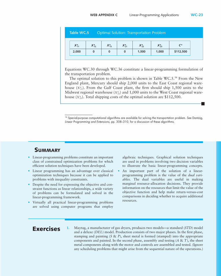
The optimal solution to this problem is shown in Table WC.5.16 From the NewEngland plant, Mercury should ship 2,000 units to the East Coast regional ware-house (X*11). From the Gulf Coast plant, the firm should ship 1,500 units to theMidwest regional warehouse (X*22) and 1,000 units to the West Coast regional ware-house (X*23). Total shipping costs of the optimal solution are $112,500.


X*11 X*12 X*13 X*21 X*22 X*23 C*

2,000 0 0 0 1,500 1,000 $112,500

Table WC.5 Optimal Solution: Transportation Problem

16 Special-purpose computational algorithms are available for solving the transportation problem. See Dantzig,Linear Programming and Extensions, pp. 308–310, for a discussion of these algorithms.

SUMMARY• Linear-programming problems constitute an important

class of constrained optimization problems for whichefficient solution techniques have been developed.

• Linear programming has an advantage over classicaloptimization techniques because it can be applied toproblems with inequality constraints.

• Despite the need for expressing the objective and con-straint functions as linear relationships, a wide varietyof problems can be formulated and solved in thelinear-programming framework.

• Virtually all practical linear-programming problemsare solved using computer programs that employ

algebraic techniques. Graphical solution techniquesare used in problems involving two decision variablesto illustrate the basic linear-programming concepts.

• An important part of the solution of a linear-programming problem is the value of the dual vari-ables. The dual variables are useful in makingmarginal resource-allocation decisions. They provideinformation on the resources that limit the value of theobjective function and help make return-versus-costcomparisons in deciding whether to acquire additionalresources.

1. Maytag, a manufacturer of gas dryers, produces two models—a standard (STD) modeland a deluxe (DEL) model. Production consists of two major phases. In the first phase,stamping and painting (S & P), sheet metal is formed (stamped) into the appropriatecomponents and painted. In the second phase, assembly and testing (A & T ), the sheetmetal components along with the motor and controls are assembled and tested. (Ignoreany scheduling problems that might arise from the sequential nature of the operations.)

Exercises


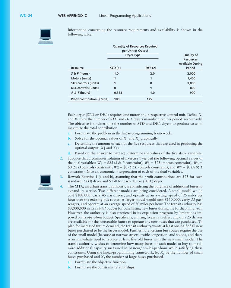
Each dryer (STD or DEL) requires one motor and a respective control unit. Define X1

and X2 to be the number of STD and DEL dryers manufactured per period, respectively.The objective is to determine the number of STD and DEL dryers to produce so as tomaximize the total contribution. a. Formulate the problem in the linear-programming framework.b. Solve for the optimal values of X1 and X2 graphically.c. Determine the amount of each of the five resources that are used in producing the

optimal output (X*1 and X*2).d. Based on the answer to part (c), determine the values of the five slack variables.

2. Suppose that a computer solution of Exercise 1 yielded the following optimal values ofthe dual variables: W*1 � $25 (S & P constraint), W*2 � $75 (motors constraint), W*3 �$0 (STD controls constraint), W*4 � $0 (DEL controls constraint), and W*5 � $0 (A & Tconstraint). Give an economic interpretation of each of the dual variables.

3. Rework Exercise 1 (a and b), assuming that the profit contributions are $75 for eachstandard (STD) dryer and $150 for each deluxe (DEL) dryer.

4. The MTA, an urban transit authority, is considering the purchase of additional buses toexpand its service. Two different models are being considered. A small model wouldcost $100,000, carry 45 passengers, and operate at an average speed of 25 miles perhour over the existing bus routes. A larger model would cost $150,000, carry 55 pas-sengers, and operate at an average speed of 30 miles per hour. The transit authority has$3,000,000 in its capital budget for purchasing new buses during the forthcoming year.However, the authority is also restricted in its expansion program by limitations im-posed on its operating budget. Specifically, a hiring freeze is in effect and only 25 driversare available for the foreseeable future to operate any new buses that are purchased. Toplan for increased future demand, the transit authority wants at least one-half of all newbuses purchased to be the larger model. Furthermore, certain bus routes require the useof the small model (because of narrow streets, traffic congestion, and so on), and thereis an immediate need to replace at least five old buses with the new small model. Thetransit authority wishes to determine how many buses of each model to buy to maxi-mize additional capacity measured in passenger-miles-per-hour while satisfying theseconstraints. Using the linear-programming framework, let X1 be the number of smallbuses purchased and X2 the number of large buses purchased.a. Formulate the objective function.b. Formulate the constraint relationships.


Quantity of Resources Required per Unit of Output

Dryer Type Quality ofResources

Available DuringResource STD (1) DEL (2) Period

S & P (hours) 1.0 2.0 2,000

Motors (units) 1 1 1,400

STD controls (units) 1 0 1,000

DEL controls (units) 0 1 800

A & T (hours) 0.333 1.0 900

Profit contribution ($/unit) 100 125

Information concerning the resource requirements and availability is shown in thefollowing table:



c. Using graphical methods, determine the optimal combination of buses to purchase.d. Formulate (but do not solve) the dual problem, and give an interpretation of the

dual variables.5. Consider the cost-minimization production problem described in Equations WC.12–

WC16.a. Graph the feasible solution space.b. Graph the objective function as a series of isocost lines.c. Using graphical methods, determine the optimal solution. Compare the graphical

solution to the computer solution given in Figure WC.8.6. Assume that the Agrex Company, a fertilizer manufacturer, wishes to determine the

profit-maximizing level of output of two products, Alphagrow (X1) and Better Grow(X2). Each pound of X1 produced and sold contributes $2 to overhead and profit,whereas X2’s contribution is $3 per pound. Additional information:• The total productive capacity of the firm is 2,000 pounds of fertilizer per week. This

capacity may be used to produce all X1, all X2, or some linear proportional mix ofthe two.

• Because of the light weight and bulk of X2 relative to X1, the packaging departmentcan handle a maximum of 2,400 pounds of X1, 1,200 pounds of X2, or some linearproportional mix of the two each week.

• Large amounts of propane are required in the production process. Because of an en-ergy shortage, the firm is limited to producing 2,100 pounds of X2, 1,400 pounds ofX1, or some linear proportional mix of the two each week.

• On the average, the firm expects to have $5,000 in cash available to meet operatingexpenses each week. Each pound of X1 produced requires an initial cash outflow of$2, whereas each pound of X2 requires an outflow of $4.a. Formulate this as a profit-maximization problem in the linear-programming

framework. Be sure to clearly specify all constraints.b. Solve for the approximate profit-maximizing levels of output of X1 and X2, using

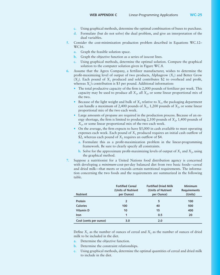
the graphical method.7. Suppose a nutritionist for a United Nations food distribution agency is concerned

with developing a minimum-cost-per-day balanced diet from two basic foods—cerealand dried milk—that meets or exceeds certain nutritional requirements. The informa-tion concerning the two foods and the requirements are summarized in the followingtable.

Fortified Cereal Fortified Dried Milk Minimum(Units of Nutrient (Units of Nutrient Requirements

Nutrient per Ounce) per Ounce) (Units)

Protein 2 5 100

Calories 100 40 500

Vitamin D 10 15 400

Iron 1 0.5 20

Cost (cents per ounce) 3.0 2.0

Define X1 as the number of ounces of cereal and X2 as the number of ounces of driedmilk to be included in the diet.a. Determine the objective function.b. Determine the constraint relationships.c. Using graphical methods, determine the optimal quantities of cereal and dried milk

to include in the diet.



d. Determine the amount of the four nutrients used in producing the optimal diet (X*1 and X*2).

e. Based on your answer to part (d), determine the values of the four surplusvariables.

8. Suppose that a computer solution of Exercise 7 yielded the following optimal values ofthe dual variables: W1* � 0 (protein constraint), W2* � 0 (calories constraint), W3* � 0.05cents (vitamin D constraint), and W4* � 2.5 cents (iron constraint). Give an economicinterpretation of each of the dual variables.

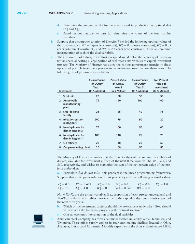
9. The government of Indula, in an effort to expand and develop the economy of the coun-try, has been allocating a large portion of each year’s tax revenues to capital investmentprojects. The Ministry of Finance has asked the various government agencies to drawup a list of possible investment projects to be undertaken over the next three years. Thefollowing list of proposals was submitted.

Present Value Present Value Present Value Net Presentof Outlay of Outlay of Outlay Value of

Year 1 Year 2 Year 3 InvestmentInvestment (In $ Million) (In $ Million) (In $ Million) (In $ Million)

1. Steel mill 20 80 50 50

2. Automobile 75 150 100 100manufacturingplant

3. Ship-docking 25 25 40 75facility

4. Irrigation system 200 75 50 20in Region 1

5. New hydroelectric 75 100 50 40dam in Region 3

6. New hydroelectric 100 110 75 75dam in Region 1

7. Oil refinery 25 40 25 60

8. Copper-smelting plant 20 50 50 50

The Ministry of Finance estimates that the present values of the amount (in millions ofdollars) available for investment in each of the next three years will be 300, 325, and350, respectively, and wishes to maximize the sum of the net present value of the pro-jects undertaken.a. Formulate (but do not solve) this problem in the linear-programming framework.Suppose that a computer solution of this problem yields the following optimal values:

X*1 � 0.0 X*2 � 0.667 X*3 � 1.0 X*4 � 0.0 X*5 � 0.0 X*6 � 1.0X*7 � 1.0 X*8 � 1.0 W*1 � 0.0 W*2 � 0.667 W*3 � 0.0

Note: X1–X8 are the primal variables (i.e., proportion of each project undertaken) andW1–W3 are the dual variables associated with the capital budget constraints in each ofthe next three years.b. Which of the investment projects should the government undertake? How should

we deal with the fractional projects in the optimal solution?c. Give an economic interpretation of the dual variables.

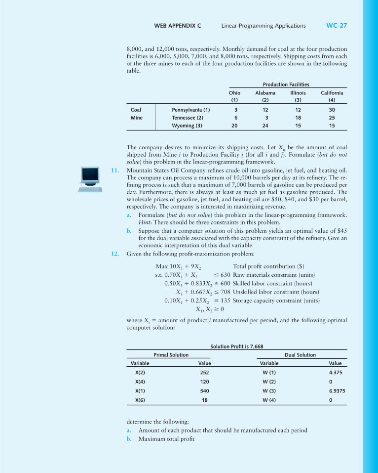
10. American Steel Company has three coal mines located in Pennsylvania, Tennessee, andWyoming. These mines supply coal to its four steel-making facilities located in Ohio,Alabama, Illinois, and California. Monthly capacities of the three coal mines are 6,000,



8,000, and 12,000 tons, respectively. Monthly demand for coal at the four productionfacilities is 6,000, 5,000, 7,000, and 8,000 tons, respectively. Shipping costs from eachof the three mines to each of the four production facilities are shown in the followingtable.

Production Facilities

Ohio Alabama Illinois California(1) (2) (3) (4)

Coal Pennsylvania (1) 3 12 12 30

Mine Tennessee (2) 6 3 18 25

Wyoming (3) 20 24 15 15

Solution Profit is 7,668

Primal Solution Dual Solution

Variable Value Variable Value

X(2) 252 W (1) 4.375

X(4) 120 W (2) 0

X(1) 540 W (3) 6.9375

X(6) 18 W (4) 0

The company desires to minimize its shipping costs. Let Xij be the amount of coalshipped from Mine i to Production Facility j (for all i and j). Formulate (but do notsolve) this problem in the linear-programming framework.

11. Mountain States Oil Company refines crude oil into gasoline, jet fuel, and heating oil.The company can process a maximum of 10,000 barrels per day at its refinery. The re-fining process is such that a maximum of 7,000 barrels of gasoline can be produced perday. Furthermore, there is always at least as much jet fuel as gasoline produced. Thewholesale prices of gasoline, jet fuel, and heating oil are $50, $40, and $30 per barrel,respectively. The company is interested in maximizing revenue. a. Formulate (but do not solve) this problem in the linear-programming framework.

Hint: There should be three constraints in this problem.b. Suppose that a computer solution of this problem yields an optimal value of $45

for the dual variable associated with the capacity constraint of the refinery. Give aneconomic interpretation of this dual variable.

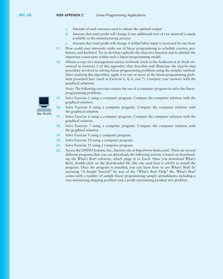
12. Given the following profit-maximization problem:

Max 10X1 � 9X2 Total profit contribution ($)s.t. 0.70X1 � X2 � 630 Raw materials constraint (units)

0.50X1 � 0.833X2 � 600 Skilled labor constraint (hours)X1 � 0.667X2 � 708 Unskilled labor constraint (hours)

0.10X1 � 0.25X2 � 135 Storage capacity constraint (units)X1, X2 � 0

where Xi � amount of product i manufactured per period, and the following optimalcomputer solution:

determine the following:a. Amount of each product that should be manufactured each periodb. Maximum total profit



c. Amount of each resource used to obtain the optimal outputd. Amount that total profit will change if one additional unit of raw material is made

available to the manufacturing processe. Amount that total profit will change if skilled labor input is increased by one hour

13. How could your university make use of linear programming to schedule courses, pro-fessors, and facilities? Try to develop explicitly the objective function and to identify theimportant constraints within such a linear-programming model.

14. Obtain a copy of a management science textbook (such as the Anderson et al. book ref-erenced in footnote 1 of this appendix) that describes and illustrates the step-by-stepprocedure involved in solving linear-programming problems using the simplex method.After studying this algorithm, apply it to one or more of the linear-programming prob-lems presented here (such as Exercise 1, 4, 6, and 7). Compare your answers with thegraphical solutions.

Note: The following exercises require the use of a computer program to solve the linear-programming problems.

15. Solve Exercise 1 using a computer program. Compare the computer solution with thegraphical solution.

16. Solve Exercise 4 using a computer program. Compare the computer solution withthe graphical solution.

17. Solve Exercise 6 using a computer program. Compare the computer solution with thegraphical solution.

18. Solve Exercise 7 using a computer program. Compare the computer solution withthe graphical solution.

19. Solve Exercise 9 using a computer program.20. Solve Exercise 10 using a computer program.21. Solve Exercise 11 using a computer program.22. Access the LINDO Systems, Inc., Internet site at http://www.lindo.com/. There are several

different programs that you can download; the following activity is based on download-ing the What’s Best! software, which plugs in to Excel. Once you download What’sBest!, double-click on the downloaded file (the one used here is wb30) to install theprogram. Once the program is installed, you can learn how to use What’s Best! byaccessing “A Simple Tutorial” by way of the “What’s Best! Help” file. What’s Best!comes with a number of sample linear programming sample spreadsheets, including acost-minimizing shipping problem and a profit-maximizing product mix problem.

(for 15–21)


Documents

21605 23 Webappendix C