Embed Size (px)
Citation preview
European Consortium for Mathematics in Industry
28th ECMI Modelling WeekFinal Report
19.07.2015—26.07.2015Lisboa, Portugal
Group 10
Mathematical Modelling ofFinancial Data in ManyDimensions
Astrid VestergrdDTU Compute, Technical University of Denmark,
Anker Engelunds Vej 1, Building 101A, 2800 Kgs. Lyngby , DenmarkCamara Mamadou,
UFR Mathematiques Informatique,University of Strasbourg 7 Rue Rene Descartes 67084 Strasbourg, France
Matilde Lopes RosaInstituto Superior Tecnico, University of Lisbon,
Rua dos Arneiros n.o 26 2.o A 1550-059 Lisboa, PortugalRamona Maraia
Department of Mathematics, Faculty of Science and Technology, Univesityof Milan, via Saldini 50 Milan, Italy
Velislav BodurovFaculty of Mathematics and Informatics, Sofia University,
5 James Bourchier Blvd., Sofia, Bulgaria
Instructor: Janusz GajdaDepartment of Pure and Applied Mathematics, Wrocaw University of
Technologyul. Wybrzee Wyspiaskiego 27 50-370 Wrocaw, Poland
2
Abstract
Forecasting stock price movements is not an easy task. The data is complexand each set of prices for a stock may have dependencies, therefore financialdata may be better modelled as multidimensional data. In this report thedata has been considered as time series, multidimensional time series. Threesets of data have been considered and modelled, that is, the stock prices ofTech companies, the price of precious metals, and finally, the behavior ofthe Portuguese inflation rate, consumption, unemployment rate and realexchange rate.We find that for the first data set, the movements are random after removingtrends and a multivariate modelling approach is not the best suited forthe problem. The second data set was more correlated and well suited formultivariate modelling, however the predictions did not do well. The thirddata was also well suited for multivariate modelling, and the final model wasable to predict the data well for the first time period but not so well for thesecond, as the financial crisis was not taken into account in the data usedfor modelling.
2 Mathematical modeling of financial data in many dimensions
10.1 Introduction
The aim of this project is to build a multivariate time series model to modelreal financial data. A time series is an ordered sequence of values of a variableat equally spaced time intervals, which is useful to see how a given variablechanges over time or how it changes compared to other variables over thesame time period. The idea is to find correlated variables and build a modelto predict the future behavior of those variables by using the dependenciesbetween them. We built three models for different data sets. First wepresent a financial model to predict stock prices of Tech companies but whichturned out to be stochastic. Secondly, we show a model to predict the priceof some precious metals (gold, silver, palladium and platinum). The lastmodel aims to predict the behavior of several Portuguese macroeconomicvariables (inflation, consumption, unemployment and real exchange rate).Finally, we discuss further work, especially regarding the two latter datasets.
10.2 Theory
VAR(p) model in the multivariate case
The vector autoregression (VAR) model is one of the most successful, flexi-ble, and easy to use models for the analysis of multivariate time series. It isan extension of the univariate autoregressive model to dynamic multivariatetime series. The VAR model has proven to be especially useful for describingthe dynamic behavior of economic and financial time series as well as forforecasting.
The model captures the relationship between different time series in time,time series observations are available for variables of interest.
VAR models are a specific case of the more general VARMA models.VARMA models for multivariate time series include the VAR structureabove along with moving average terms for each variable. More generallyyet, these are special cases of ARMAX models that allow for the addition ofother predictors that are outside the multivariate set of principal interest.
The structure is that each variable is a linear function of past lags ofitself and past lags of the other variables. In general, for a VAR(p) model,the first p lags of each variable in the system would be used as regressionpredictors for each variable.
Let
Yt = (y1t, y2t, ..., ynt)′,
28th ECMI Modelling Week 3
denote an (n× 1) vector of n different time series variables.The basic p-lag VAR(p) model has the form
Yt = c+ Π1Yt−1 + Π2Yt−2 + · · ·+ ΠpYt−p + εt, t = p, . . . , T,
where Πi are (n×n) coefficient matrices and εt is an (n×1) unobservable zeromean white noise vector process (uncorrelated or independent) with timeinvariant covariance matrix Σ. εt is Gaussian white noise, εt ∼ N(0,Πε) ∀tand εt and εs are independent for s 6= t.
In economic time series, the white noise series is often thought of asrepresenting innovations, or shocks. That is, εt represents those aspects ofthe time series of interest which could not have been predicted in advance.In lag operator notation, the VAR(p) is written as
Π(L)Yt = c+ εt,
where Π(L) = In −Π1z − · · · −Πpzp.
The VAR(p) is stable if the root of
det(In −Π1z − ...−Πpzp) = 0,
lies outside the complex unit circle (have modulus greater than one),or,equivalently, if the eigenvalues of the companion matrix
F =
Π1 Π2 . . . Πn
In 0 . . . 0
0. . . 0
...0 0 In 0
,have modulus less than one.Assuming that the process has been initialized in the infinite past, then astable VAR(p) process is stationary and ergodic with time invariant means,variances, and autocovariances.
Parameter estimation
Given a sample of size T, y1, . . . , yT , and p presample vectors, yp−1, . . . , y0,the parameters can be estimated efficiently by ordinary least squares (OLS)for each equation separately.
The VAR model should include all variables which the theory indicatesare relevant and we should choose the lag length which has a high likelihoodof capturing all of the dynamics. Once these values have been set, either ageneral-to-specific search can be conducted or an information criteria (IC)
4 Mathematical modeling of financial data in many dimensions
can be used to select the appropriate lag length.In the VAR case, the main information criteria are:
Akaike information criterion (AIC) is a measure of the relative qual-ity of statistical models. Given a set of candidate models for the data, thepreferred model is the one with the minimum AIC value.
Bayesian information criterion (BIC) is a criterion for model se-lection among a finite set of models. The model with the lowest BIC ispreferred; it is based, in part, on the likelihood function and it is closelyrelated to the Akaike information criterion (AIC).
Hannan – Quinn information criterion (HQC) is a criterion formodel selection. It is an alternative to the Akaike information criterion(AIC) and the Bayesian information criterion (BIC).
The lag length should be chosen to minimize one of these criteria, andthe BIC will always choose a (weakly) smaller model than the HQC whichin turn will select a (weakly) smaller model than the AIC.
Random Walk
A random walk is a mathematical formalization of a path that consists of asuccession of random steps. Often, the walk is in discrete time, and indexedby the natural numbers, as in X0, X1, X2, . . . . However, some walks taketheir steps at random times, and in that case the position Xt is definedfor the continuum of times t ≥ 0. Specific cases or limits of random walksinclude the Levy flight. Random walks are related to the diffusion modelsand are a fundamental topic in discussions of Markov processes.
In economics, the ”random walk hypothesis” is used to model sharesprices and other factors. Empirical studies found some deviations from thistheoretical model, especially in short term and long term correlations.
10.3 A financial model
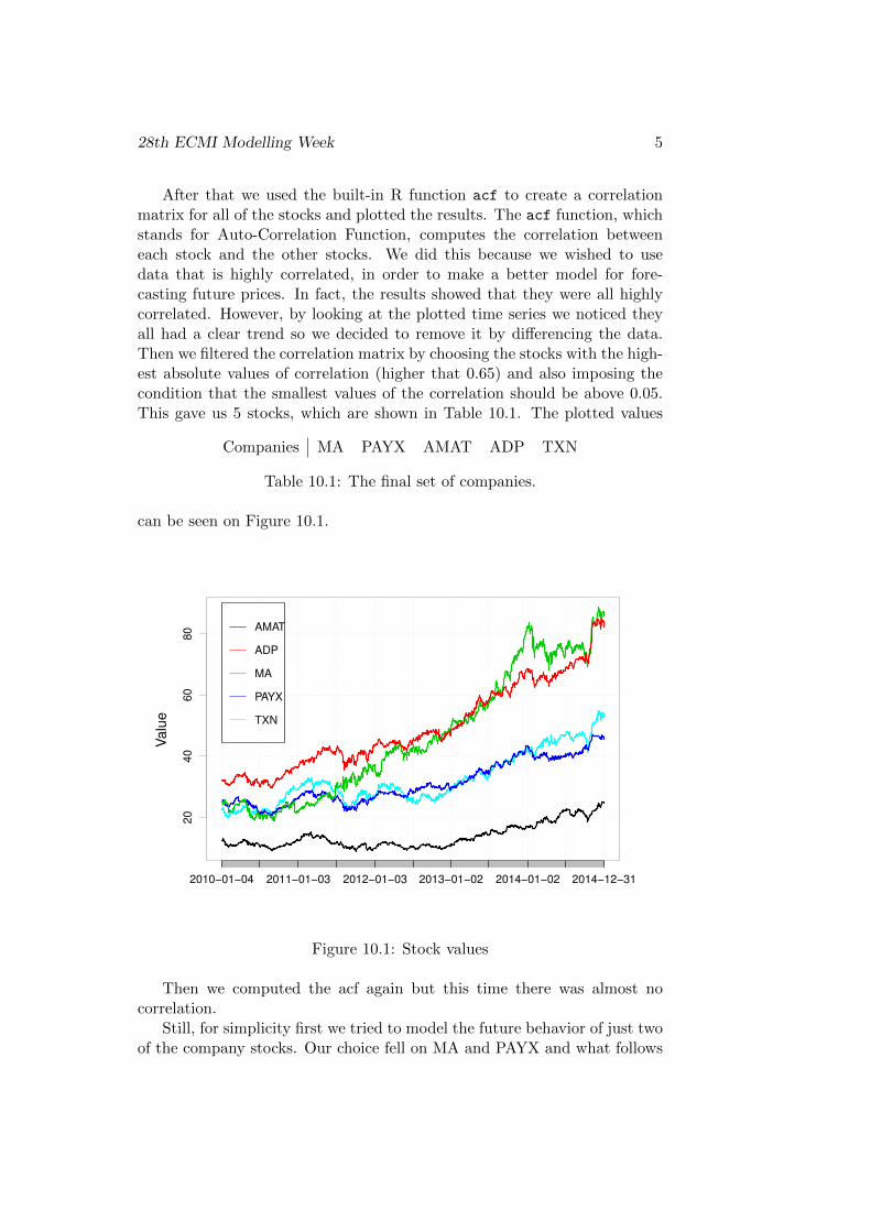
The data used for this project has been gathered from Yahoo Finance. Westarted with 50 tech companies listed on NASDAQ from [5], and eliminatedthe companies that did not have data for the entire period we are considering,leaving 46 to be used. The chosen period is five years long and goes from01/01/2010 to 31/12/2014 and the data is the adjusted daily closing prices.For this part of the data preparation we have used first Matlab to get thedata from Yahoo and build a matrix with the stocks and the dates, and thenwe used R to analyse the data. In R we transformed the data into a timeseries object with the function ts.
28th ECMI Modelling Week 5
After that we used the built-in R function acf to create a correlationmatrix for all of the stocks and plotted the results. The acf function, whichstands for Auto-Correlation Function, computes the correlation betweeneach stock and the other stocks. We did this because we wished to usedata that is highly correlated, in order to make a better model for fore-casting future prices. In fact, the results showed that they were all highlycorrelated. However, by looking at the plotted time series we noticed theyall had a clear trend so we decided to remove it by differencing the data.Then we filtered the correlation matrix by choosing the stocks with the high-est absolute values of correlation (higher that 0.65) and also imposing thecondition that the smallest values of the correlation should be above 0.05.This gave us 5 stocks, which are shown in Table 10.1. The plotted values
Companies MA PAYX AMAT ADP TXN
Table 10.1: The final set of companies.
can be seen on Figure 10.1.
2010−01−04 2011−01−03 2012−01−03 2013−01−02 2014−01−02 2014−12−31
20
40
60
80
Valu
e
AMAT
ADP
MA
PAYX
TXN
Figure 10.1: Stock values
Then we computed the acf again but this time there was almost nocorrelation.
Still, for simplicity first we tried to model the future behavior of just twoof the company stocks. Our choice fell on MA and PAYX and what follows
6 Mathematical modeling of financial data in many dimensions
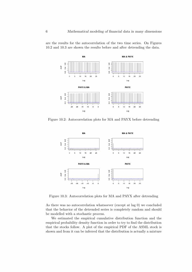
are the results for the autocorrelation of the two time series. On Figures10.2 and 10.3 are shown the results before and after detrending the data.
Figure 10.2: Autocorrelation plots for MA and PAYX before detrending
Figure 10.3: Autocorrelation plots for MA and PAYX after detrending
As there was no autocorrelation whatsoever (except at lag 0) we concludedthat the behavior of the detrended series is completely random and shouldbe modelled with a stochastic process.
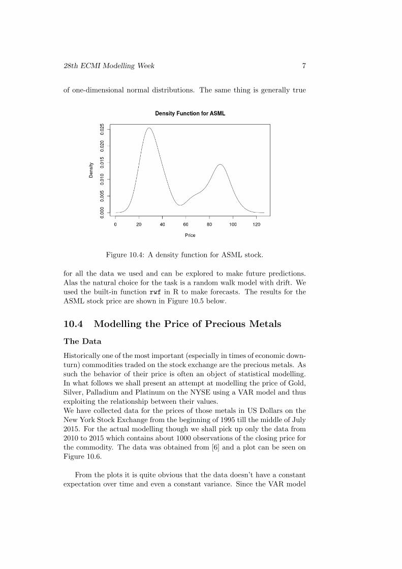
We estimated the empirical cumulative distribution function and theempirical probability density function in order to try to find the distributionthat the stocks follow. A plot of the empirical PDF of the ASML stock isshown and from it can be inferred that the distribution is actually a mixture
28th ECMI Modelling Week 7
of one-dimensional normal distributions. The same thing is generally true
Figure 10.4: A density function for ASML stock.
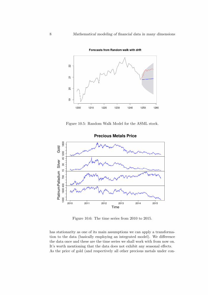
for all the data we used and can be explored to make future predictions.Alas the natural choice for the task is a random walk model with drift. Weused the built-in function rwf in R to make forecasts. The results for theASML stock price are shown in Figure 10.5 below.
10.4 Modelling the Price of Precious Metals
The Data
Historically one of the most important (especially in times of economic down-turn) commodities traded on the stock exchange are the precious metals. Assuch the behavior of their price is often an object of statistical modelling.In what follows we shall present an attempt at modelling the price of Gold,Silver, Palladium and Platinum on the NYSE using a VAR model and thusexploiting the relationship between their values.We have collected data for the prices of those metals in US Dollars on theNew York Stock Exchange from the beginning of 1995 till the middle of July2015. For the actual modelling though we shall pick up only the data from2010 to 2015 which contains about 1000 observations of the closing price forthe commodity. The data was obtained from [6] and a plot can be seen onFigure 10.6.
From the plots it is quite obvious that the data doesn’t have a constantexpectation over time and even a constant variance. Since the VAR model
8 Mathematical modeling of financial data in many dimensions
Figure 10.5: Random Walk Model for the ASML stock.
12
00
18
00
Go
ld
15
30
45
Silve
r
40
07
00
Pa
lla
diu
m
10
00
16
00
2010 2011 2012 2013 2014 2015
Pla
tinu
m
Time
Precious Metals Price
Figure 10.6: The time series from 2010 to 2015.
has stationarity as one of its main assumptions we can apply a transforma-tion to the data (basically employing an integrated model). We differencethe data once and these are the time series we shall work with from now on.It’s worth mentioning that the data does not exhibit any seasonal effects.As the price of gold (and respectively all other precious metals under con-
28th ECMI Modelling Week 9
sideration) is highly influenced by the value of the US Dollar compared toother world currencies it seemed natural to try and incorporate that valueinto the model in some way. Overall though this turned out to be of almostno use as it did not improve the strength of our model in any meaningfulway while introducing yet another set of parameters. For the sake of sim-plicity this idea was abandoned and we proceed to model only the prices ofthe four metals.
Model Selection
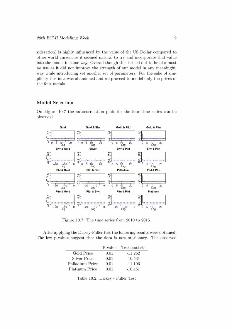
On Figure 10.7 the autocorrelation plots for the four time series can beobserved.
0 5 10 20−0
.20
.8
Lag
AC
F
Gold
0 5 10 20−0
.20
.8
Lag
Gold & Slvr
0 5 10 20−0
.20
.8
Lag
Gold & Plld
0 5 10 20−0
.20
.8
Lag
Gold & Pltn
−20 −10 0−0.2
0.8
Lag
AC
F
Slvr & Gold
0 5 10 20−0.2
0.8
Lag
Silver
0 5 10 20−0.2
0.8
Lag
Slvr & Plld
0 5 10 20−0.2
0.8
Lag
Slvr & Pltn
−20 −10 0−0
.20
.8
Lag
AC
F
Plld & Gold
−20 −10 0−0
.20
.8
Lag
Plld & Slvr
0 5 10 20−0
.20
.8
Lag
Palladium
0 5 10 20−0
.20
.8
Lag
Plld & Pltn
−20 −10 0−0
.20
.8
Lag
AC
F
Pltn & Gold
−20 −10 0−0
.20
.8
Lag
Pltn & Slvr
−20 −10 0−0
.20
.8
Lag
Pltn & Plld
0 5 10 20−0
.20
.8
Lag
Platinum
Figure 10.7: The time series from 2010 to 2015.
After applying the Dickey-Fuller test the following results were obtained:The low p-values suggest that the data is now stationary. The observed
P-value Test statistic
Gold Price 0.01 -11.262Silver Price 0.01 -10.531
Palladium Price 0.01 -11.106Platinum Price 0.01 -10.461
Table 10.2: Dickey - Fuller Test
10 Mathematical modeling of financial data in many dimensions
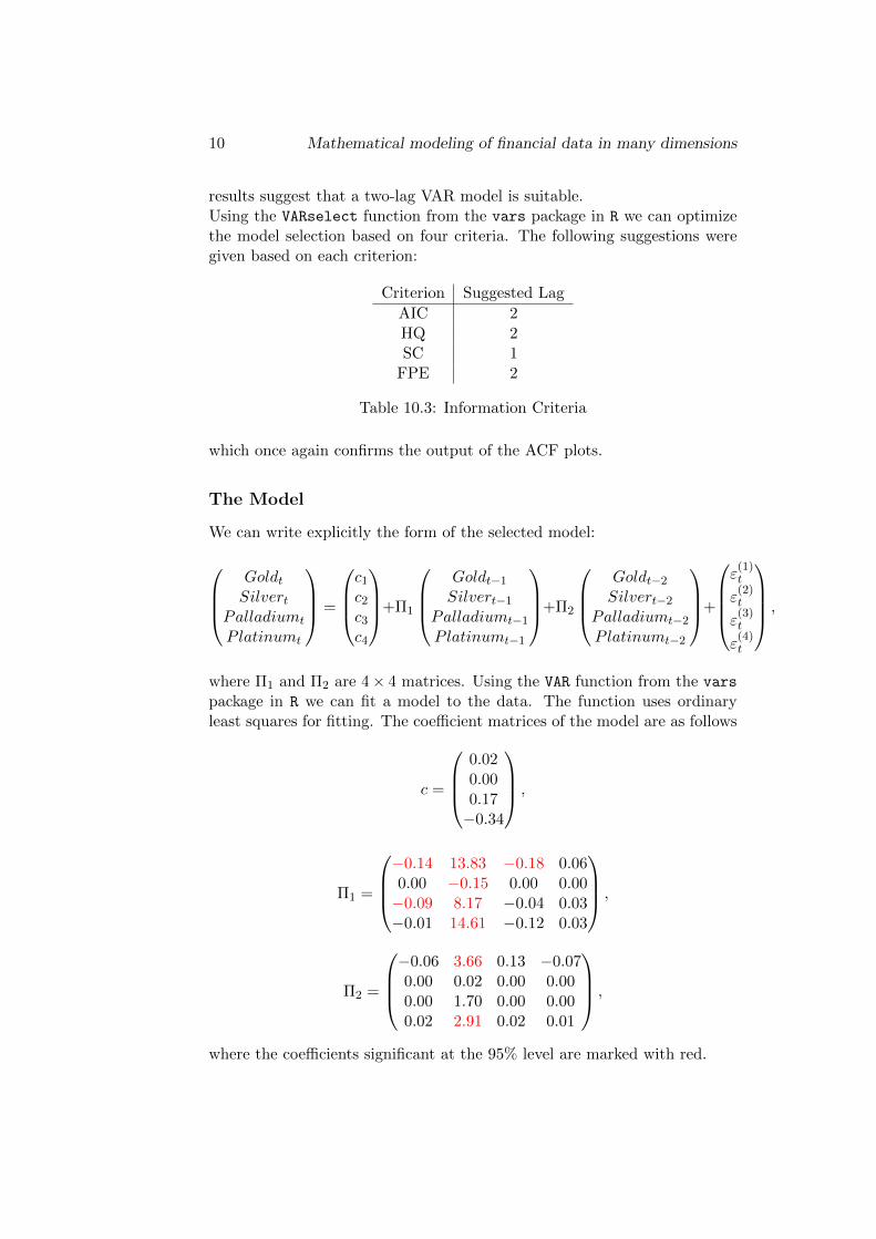
results suggest that a two-lag VAR model is suitable.Using the VARselect function from the vars package in R we can optimizethe model selection based on four criteria. The following suggestions weregiven based on each criterion:
Criterion Suggested Lag
AIC 2HQ 2SC 1
FPE 2
Table 10.3: Information Criteria
which once again confirms the output of the ACF plots.
The Model
We can write explicitly the form of the selected model:
GoldtSilvert
Palladiumt
Platinumt
=
c1
c2
c3
c4
+Π1
Goldt−1
Silvert−1
Palladiumt−1
Platinumt−1
+Π2
Goldt−2
Silvert−2
Palladiumt−2
Platinumt−2
+
ε
(1)t
ε(2)t
ε(3)t
ε(4)t
,
where Π1 and Π2 are 4× 4 matrices. Using the VAR function from the vars
package in R we can fit a model to the data. The function uses ordinaryleast squares for fitting. The coefficient matrices of the model are as follows
c =
0.020.000.17−0.34
,
Π1 =
−0.14 13.83 −0.18 0.060.00 −0.15 0.00 0.00−0.09 8.17 −0.04 0.03−0.01 14.61 −0.12 0.03
,
Π2 =
−0.06 3.66 0.13 −0.070.00 0.02 0.00 0.000.00 1.70 0.00 0.000.02 2.91 0.02 0.01
,
where the coefficients significant at the 95% level are marked with red.
28th ECMI Modelling Week 11
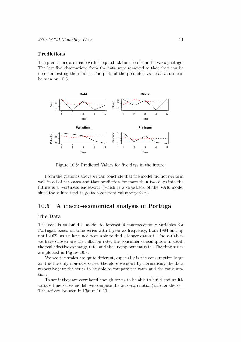
Predictions
The predictions are made with the predict function from the vars package.The last five observations from the data were removed so that they can beused for testing the model. The plots of the predicted vs. real values canbe seen on 10.8.
Gold
Time
Gold
1 2 3 4 5
−10
0
Silver
Time
Silver
1 2 3 4 5
−0.3
0.0
Palladium
Time
Palladiu
m
1 2 3 4 5
−20
0
Platinum
Time
Pla
tinum
1 2 3 4 5
−15
015
Figure 10.8: Predicted Values for five days in the future.
From the graphics above we can conclude that the model did not performwell in all of the cases and that prediction for more than two days into thefuture is a worthless endeavour (which is a drawback of the VAR modelsince the values tend to go to a constant value very fast).
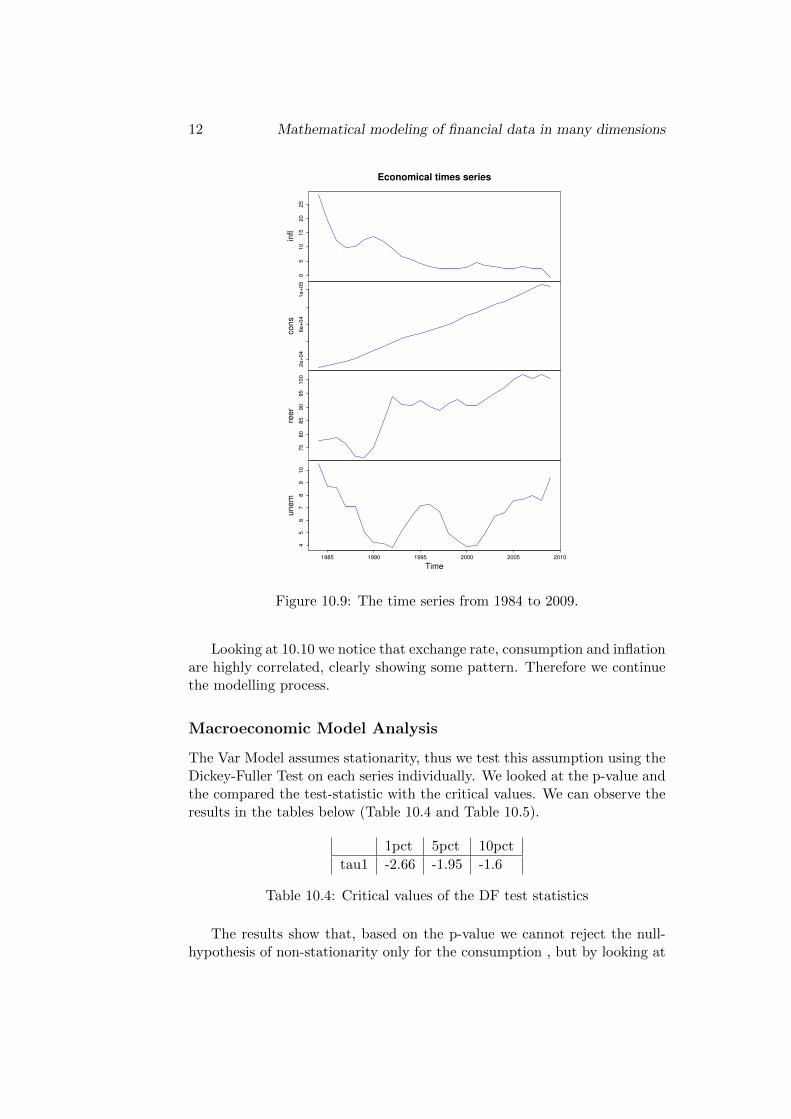
10.5 A macro-economical analysis of Portugal
The Data
The goal is to build a model to forecast 4 macroeconomic variables forPortugal, based on time series with 1 year as frequency, from 1984 and upuntil 2009, as we have not been able to find a longer dataset. The variableswe have chosen are the inflation rate, the consumer consumption in total,the real effective exchange rate, and the unemployment rate. The time seriesare plotted in Figure 10.9.
We see the scales are quite different, especially is the consumption largeas it is the only non-rate series, therefore we start by normalising the datarespectively to the series to be able to compare the rates and the consump-tion.
To see if they are correlated enough for us to be able to build and multi-variate time series model, we compute the auto-correlation(acf) for the set.The acf can be seen in Figure 10.10.
12 Mathematical modeling of financial data in many dimensions
05
10
15
20
25
infl
2e
+0
46
e+
04
1e
+0
5
cons
75
80
85
90
95
10
0
reer
45
67
89
10
1985 1990 1995 2000 2005 2010
unem
Time
Economical times series
Figure 10.9: The time series from 1984 to 2009.
Looking at 10.10 we notice that exchange rate, consumption and inflationare highly correlated, clearly showing some pattern. Therefore we continuethe modelling process.
Macroeconomic Model Analysis
The Var Model assumes stationarity, thus we test this assumption using theDickey-Fuller Test on each series individually. We looked at the p-value andthe compared the test-statistic with the critical values. We can observe theresults in the tables below (Table 10.4 and Table 10.5).
1pct 5pct 10pct
tau1 -2.66 -1.95 -1.6
Table 10.4: Critical values of the DF test statistics
The results show that, based on the p-value we cannot reject the null-hypothesis of non-stationarity only for the consumption , but by looking at
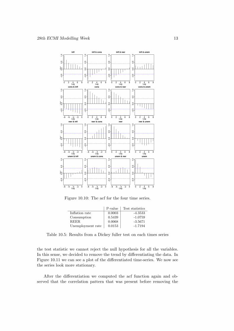
28th ECMI Modelling Week 13
0 2 4 6 8
−0.5
0.0
0.5
1.0
Lag
AC
F
infl
0 2 4 6 8−
0.5
0.0
0.5
1.0
Lag
infl & cons
0 2 4 6 8
−0.5
0.0
0.5
1.0
Lag
infl & reer
0 2 4 6 8
−0.5
0.0
0.5
1.0
Lag
infl & unem
−8 −6 −4 −2 0
−0.5
0.0
0.5
1.0
Lag
AC
F
cons & infl
0 2 4 6 8
−0.5
0.0
0.5
1.0
Lag
cons
0 2 4 6 8
−0.5
0.0
0.5
1.0
Lag
cons & reer
0 2 4 6 8
−0.5
0.0
0.5
1.0
Lag
cons & unem
−8 −6 −4 −2 0
−0.5
0.0
0.5
1.0
Lag
AC
F
reer & infl
−8 −6 −4 −2 0
−0.5
0.0
0.5
1.0
Lag
reer & cons
0 2 4 6 8
−0.5
0.0
0.5
1.0
Lag
reer
0 2 4 6 8
−0.5
0.0
0.5
1.0
Lag
reer & unem
−8 −6 −4 −2 0
−0.5
0.0
0.5
1.0
Lag
AC
F
unem & infl
−8 −6 −4 −2 0
−0.5
0.0
0.5
1.0
Lag
unem & cons
−8 −6 −4 −2 0
−0.5
0.0
0.5
1.0
Lag
unem & reer
0 2 4 6 8
−0.5
0.0
0.5
1.0
Lag
unem
Figure 10.10: The acf for the four time series.
P-value Test statistics
Inflation rate 0.0003 -4.3533Consumption 0.5439 -1.0759REER 0.0068 -3.5671Unemployment rate 0.0153 -1.7194
Table 10.5: Results from a Dickey fuller test on each times series
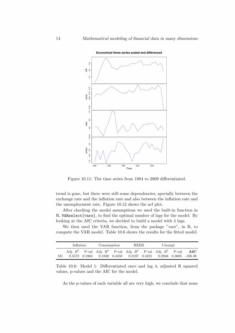
the test statistic we cannot reject the null hypothesis for all the variables.In this sense, we decided to remove the trend by differentiating the data. InFigure 10.11 we can see a plot of the differentiated time-series. We now seethe series look more stationary.
After the differentiation we computed the acf function again and ob-served that the correlation pattern that was present before removing the
14 Mathematical modeling of financial data in many dimensions
−1
.0−
0.5
0.0
infl
−0
.05
0.0
50
.10
0.1
5
cons
−0
.50
.00
.51
.0
reer
−1
.0−
0.5
0.0
0.5
1.0
1985 1990 1995 2000 2005
unem
Time
Economical times series scaled and differenced
Figure 10.11: The time series from 1984 to 2009 differentiated.
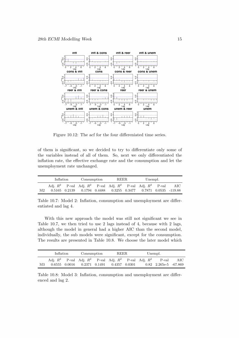
trend is gone, but there were still some dependencies, specially between theexchange rate and the inflation rate and also between the inflation rate andthe unemployment rate. Figure 10.12 shows the acf plot.
After checking the model assumptions we used the built-in function inR, VARselect{vars}, to find the optimal number of lags for the model. Bylooking at the AIC criteria, we decided to build a model with 4 lags.
We then used the VAR function, from the package ”vars”, in R, tocompute the VAR model. Table 10.6 shows the results for the fitted model.
Inflation Consumption REER Unempl.
Adj. R2 P-val Adj. R2 P-val Adj. R2 P-val Adj. R2 P-val AICM1 0.5572 0.1864 0.1838 0.4458 0.2187 0.4221 0.2946 0.3695 -106.38
Table 10.6: Model 1: Differentiated once and lag 4, adjusted R squaredvalues, p-values and the AIC for the model.
As the p-values of each variable all are very high, we conclude that none
28th ECMI Modelling Week 15
0 2 4 6
−0.5
0.5
Lag
AC
F
infl
0 2 4 6
−0.5
0.5
Lag
infl & cons
0 2 4 6
−0.5
0.5
Lag
infl & reer
0 2 4 6
−0.5
0.5
Lag
infl & unem
−7 −5 −3 −1
−0.5
0.5
Lag
AC
F
cons & infl
0 2 4 6−
0.5
0.5
Lag
cons
0 2 4 6
−0.5
0.5
Lag
cons & reer
0 2 4 6
−0.5
0.5
Lag
cons & unem
−7 −5 −3 −1
−0.5
0.5
Lag
AC
F
reer & infl
−7 −5 −3 −1
−0.5
0.5
Lag
reer & cons
0 2 4 6
−0.5
0.5
Lag
reer
0 2 4 6
−0.5
0.5
Lag
reer & unem
−7 −5 −3 −1
−0.5
0.5
Lag
AC
F
unem & infl
−7 −5 −3 −1
−0.5
0.5
Lag
unem & cons
−7 −5 −3 −1
−0.5
0.5
Lag
unem & reer
0 2 4 6
−0.5
0.5
Lag
unem
Figure 10.12: The acf for the four differeniated time series.
of them is significant, so we decided to try to differentiate only some ofthe variables instead of all of them. So, next we only differentiated theinflation rate, the effective exchange rate and the consumption and let theunemployment rate unchanged.
Inflation Consumption REER Unempl.
Adj. R2 P-val Adj. R2 P-val Adj. R2 P-val Adj. R2 P-val AICM2 0.5165 0.2139 0.1794 0.4488 0.3255 0.3477 0.7871 0.0535 -119.88
Table 10.7: Model 2: Inflation, consumption and unemployment are differ-entiated and lag 4.
With this new approach the model was still not significant we see inTable 10.7, we then tried to use 2 lags instead of 4, because with 2 lags,although the model in general had a higher AIC than the second model,individually, the sub models were significant, except for the consumption.The results are presented in Table 10.8. We choose the later model which
Inflation Consumption REER Unempl.
Adj. R2 P-val Adj. R2 P-val Adj. R2 P-val Adj. R2 P-val AICM3 0.6555 0.0016 0.2371 0.1491 0.4357 0.0301 0.82 2.265e-5 -67.869
Table 10.8: Model 3: Inflation, consumption and unemployment are differ-enced and lag 2.
16 Mathematical modeling of financial data in many dimensions
consists ofinfltconstreertuenmt
=
c1
c2
c3
c4
+ Π1
inflt−1
const−1
reert−1
unemt−1
+ Π2
inflt−2
const−2
reert−2
unemt−2
+
ε
(1)t
ε(2)t
ε(3)t
ε(4)t
, (10.1)
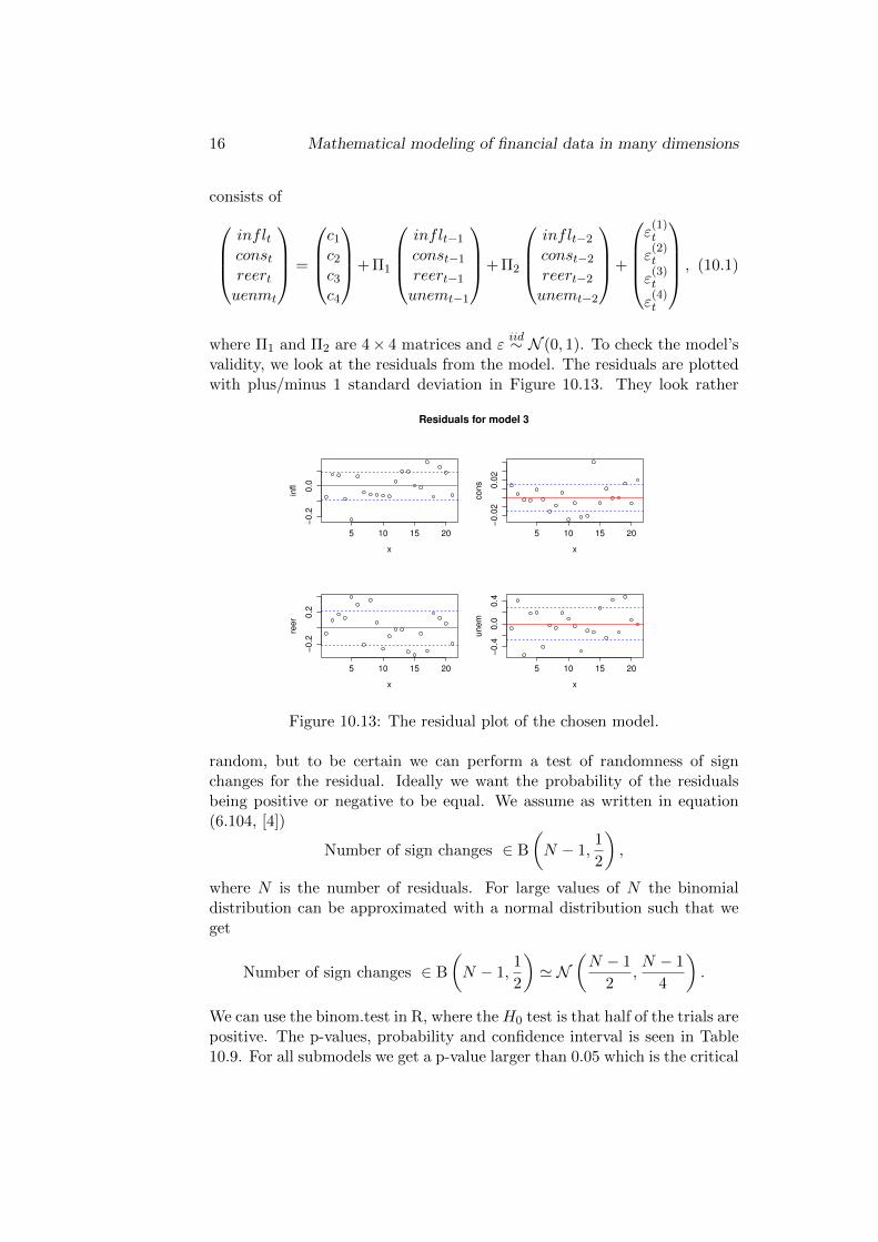
where Π1 and Π2 are 4× 4 matrices and εiid∼ N (0, 1). To check the model’s
validity, we look at the residuals from the model. The residuals are plottedwith plus/minus 1 standard deviation in Figure 10.13. They look rather
5 10 15 20
−0
.20
.0
x
infl
5 10 15 20
−0
.02
0.0
2
x
co
ns
5 10 15 20
−0
.20
.2
x
ree
r
5 10 15 20
−0
.40
.00
.4
x
un
em
Residuals for model 3
Figure 10.13: The residual plot of the chosen model.
random, but to be certain we can perform a test of randomness of signchanges for the residual. Ideally we want the probability of the residualsbeing positive or negative to be equal. We assume as written in equation(6.104, [4])
Number of sign changes ∈ B
(N − 1,
1
2
),
where N is the number of residuals. For large values of N the binomialdistribution can be approximated with a normal distribution such that weget
Number of sign changes ∈ B
(N − 1,
1
2
)' N
(N − 1
2,N − 1
4
).
We can use the binom.test in R, where the H0 test is that half of the trials arepositive. The p-values, probability and confidence interval is seen in Table10.9. For all submodels we get a p-value larger than 0.05 which is the critical
28th ECMI Modelling Week 17
number. Since it is larger than 0.05 we cannot reject the null hypothesis.From the output we also get the 95 % confidence interval, which is the 95% CI for where the true probability for success lies. We get a probability ofsuccess on 0.5 and 0.6. This probability lies within the confidence intervaland is therefore accepted. We notice it is close to the 0.5 that we assumed.
Parameter Lower bound Upper bound Probability P-valueof success
Infl. 0.2719578 0.7280422 0.5 1Cons. 0.3605426 0.8088099 0.6 0.5034REER 0.3605426 0.8088099 0.6 0.5034Unem 0.3605426 0.8088099 0.6 0.5034
Table 10.9: Result of test for sign change using N .
From the residual analysis we conclude that the residuals are randomand the assumptions about this are kept.
The final model coefficients are
c =
0.180.15−0.59−0.83
,
Π1 =
0.84 2.13 −0.13 0.040.05 0.06 0.01 −0.01−0.82 5.72 0.11 −0.04−0.01 −5.01 −0.04 1.19
,
Π2 =
−0.35 −3.93 0.11 −0.060.04 −0.12 0.03 0.020.76 0.51 −0.63 0.05−0.04 11.08 0.20 −0.35
,
where the numbers in red are significant at a 95%-level.
Predicting
When the model has been validated a prediction can be made. We haveused the predict function in the ”vars” package in R. We remove the lasttwo observations from the data to use as a ”test” set, leaving us with only23 observations for predicting. The prediction and a 95% confidence intervalcan be seen in Figure 10.14.
We notice that the model predicts the inflation rate, the consumptionand the unemployment rate are predicted quite well for the first period.The second prediction is only close for the inflation rate. We predict for the
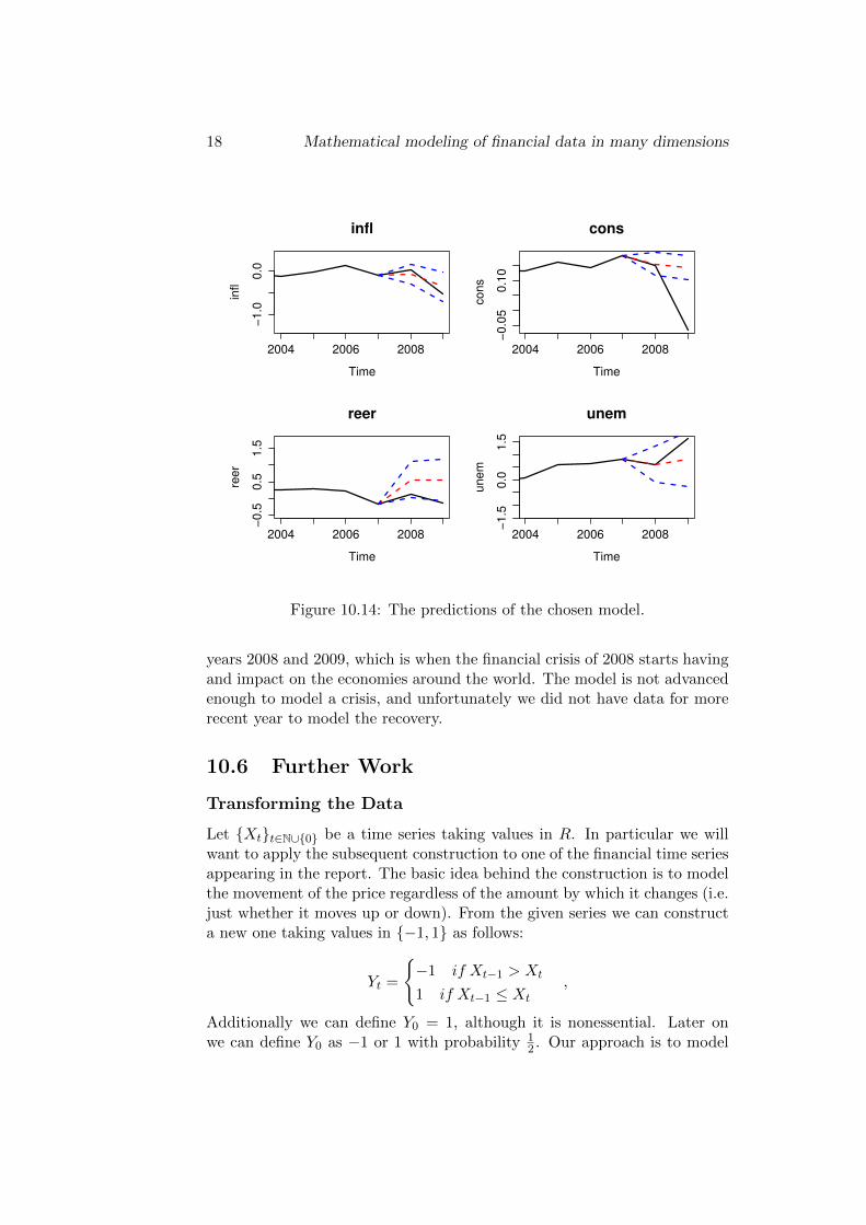
18 Mathematical modeling of financial data in many dimensions
infl
Time
infl
2004 2006 2008
−1
.00
.0
cons
Time
co
ns
2004 2006 2008
−0
.05
0.1
0
reer
Time
ree
r
2004 2006 2008
−0
.50
.51
.5
unem
Time
un
em
2004 2006 2008
−1
.50
.01
.5
Figure 10.14: The predictions of the chosen model.
years 2008 and 2009, which is when the financial crisis of 2008 starts havingand impact on the economies around the world. The model is not advancedenough to model a crisis, and unfortunately we did not have data for morerecent year to model the recovery.
10.6 Further Work
Transforming the Data
Let {Xt}t∈N∪{0} be a time series taking values in R. In particular we willwant to apply the subsequent construction to one of the financial time seriesappearing in the report. The basic idea behind the construction is to modelthe movement of the price regardless of the amount by which it changes (i.e.just whether it moves up or down). From the given series we can constructa new one taking values in {−1, 1} as follows:
Yt =
{−1 if Xt−1 > Xt
1 if Xt−1 ≤ Xt
,
Additionally we can define Y0 = 1, although it is nonessential. Later onwe can define Y0 as −1 or 1 with probability 1
2 . Our approach is to model
28th ECMI Modelling Week 19
{Yt}t∈N∪{0} instead of {Xt}t∈N∪{0}.
The Poisson Process and the Telegraphic Process
Let Nt be a Poisson process with intensity λ. An appropriate model for Ytis something in the lines of (−1)Nt . Now the parameter λ is what remainsto be estimated from the data. Having done that we can build a model ofthe stock price and make predictions employing a monte carlo simulation.If we already have an estimate of the parameter λ we can consider as avery crude approximation to the stock price at time t given by the followingprocess
Zt = v ·btc∑i=0
(−1)Ni ,
where v is the amount by which the value of the time series changes (in ourcase v = 1). Further we can consider the stochastic process
At = A0(µt+ σZt).
The parameters µ and σ can be estimated based on our knowledge of Ztat certain points in time using OLS. This process can be used as a suitablemodel for the stock price.
Estimation of the Parameter λ
According to [2] such an estimate can be obtained explicitly.Let {Xi}ni=0 be the n available observations (we shall assume observationsequidistant in time). Letm2 = 1
n
∑ni=1(Xi−Xi−1) be the quadratic variation
of the series up to time n. Then the following estimator can be considered
λ = argminλ
{m2 −
v2
2
(∆− 1− e−2λ∆
2λ
)},
where v is the constant amount with which the price moves and ∆ is thestep size (in our case 1 day). Using a numerical procedure we can get anapproximation to the real value of λ which can subsequently be used in themodels discussed.
20 Mathematical modeling of financial data in many dimensions
10.7 Appendix
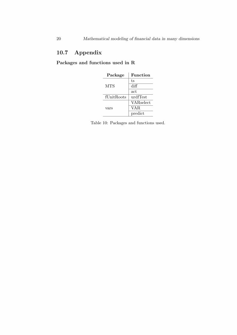
Packages and functions used in R
Package Function
MTStsdiffact
fUnitRoots urdfTest
varsVARselectVARpredict
Table 10: Packages and functions used.
Bibliography
[1] Brockwell, PJ and Davis, RA. Introduction to Time Series andForecasting. Springer Texts in Statistics. Springer, 2002.
[2] De Gregorio, A and Iacus, S. Parametric Estimation for the Stan-dard and Geometric Telegraph Process Observed at Discrete Times. 2013.
[3] Ltkepo, H. New Introduction to Multiple Time Series Analysis.Springer, 2005.
[4] Madsen, H. Time Series Analysis. Texts in Statistics Science. Chapmanand Hall, 2008.
[5] Navellier, L. Stocks to Buy and Sell: Ratings for the Top 50 TechStocks kernel description, 2010.URL http://www.nasdaq.com/article/
stocks-to-buy-and-sell-ratings-for-the-top-50-tech-stocks-cm18960
[6] Quandl.URL https://www.quandl.com/collections/markets
21

![ECMI Updates (1/2018) · Programmes, job announcements. [Read more] Our activities? Check out the ECMI Public Calendar to see what we do, where and when. [Read more] For other news](https://img.pdfslide.net/doc/110x75/5fc855d7497e284bc460ba45/ecmi-updates-12018-programmes-job-announcements-read-more-our-activities.jpg)