3 – DIMENSIONAL COMPUTATIONAL ANALYSIS OF …eprints.usm.my/8922/1/3_–_DIMENSIONAL... · 1.5 Literature Reviews 6 CHAPTER 2: THEORY: COMPUTATIONAL SCHEME 2.1 Finite ... 1.50 Gauge

3 – DIMENSIONAL COMPUTATIONAL ANALYSIS OF FLUID FLOW AROUND MICRO FLOW SENSOR AT DIFFERENT

POSITIONS AND PILLAR ARRANGEMENTS

TONY TAN HIN JOO

UNIVERSITI SAINS MALAYSIA 2008

ii

ACKNOWLEDGEMENT

I would like to take this opportunity to express my special thanks to my

supervisor, Dr. Mohd. Zulkifly Bin Abdullah, who gave me a lot of advice and guidance

in conducting the research.

Again, I also want to thank my supervisor as well as USM for giving financial

support to me during my study.

Besides this, special thanks are also given to Dr. Al – Badlishah, Mr. Roslan

(Technician) and Mr. Amir (Technician) from Electrical And Electronic Engineering

School, who gave me technical supports for completion of the research.

Lastly, I would like to thank my parents who gave me continuous supports during

the whole research.

iii

CONTENTS Page ACKNOWLEDGEMENT ii

TABLE OF CONTENTS iii

LIST OF TABLES v

LIST OF FIGURES vi

LIST OF ABBREVIATION xiii

NOMENCLATURES xiii

LIST OF REFERENCES xiv

ABSTRAK xv

ABSTRACT xvii

CHAPTER 1: INTRODUCTION

1.1 General 1

1.2 Objectives 3

1.3 Problem Statement 4

1.4 Principle Of Thermal Mass Flow Meters For Conventional

Flow Sensor 4

1.5 Literature Reviews 6

CHAPTER 2: THEORY: COMPUTATIONAL SCHEME

2.1 Finite Difference Method 47

2.2 First – Order Upwind Scheme and Third – Order Upwind Scheme 49

2.3 MAC Method 60

2.4 Initial Boundary Conditions 63

CHAPTER 3: RESULTS AND DISCUSSION

3.1 Fluid Flow Around Micro Flow Sensor In Rectangular Channel 70

3.2 Result Verification 73

3.3 Optimization of Sensor Height Position 75

iv

3.4 Analysis of Air Cavity Effect in Sensor Body 76

3.5 Micro Flow Sensor Without Pillar 79

3.5.1 Reynolds Number Effect On Micro Flow Sensor Without Pillar 79

3.5.2 Comparison of Horizontal Position and Diagonal Position For

Micro Flow Sensor Without Pillar 85

3.6 Micro Flow Sensor With Single Pillar 87

3.6.1 Reynolds Number Effect On Micro Flow Sensor With Single

Pillar 87


Micro Flow Sensor With Single Pillar 93

3.7 Micro Flow Sensor With Two Pillars 94

3.7.1 Reynolds Number Effect On Micro Flow Sensor With Two

Pillars 94

3.7.2 Comparison of Different Positions For Micro Flow Sensor

With Two Pillars 101

3.8 Micro Flow Sensor With Four Pillars 103

3.8.1 Reynolds Number Effect On Micro Flow Sensor With Four

Pillars 103


Micro Flow Sensor With Four Pillars 110

3.9 Comparison Of Boundary Layers Thickness Among Various Sensor

Designs For Various Fluid Velocity At Diagonal Position 111

CHAPTER 4: CONCLUSION

4.1 Conclusion 114

REFERENCES 116

v

LIST OF TABLES Page 1.1 Measured and predicted overall pressure drops in the S5 (‘short’)

micro channels 25

vi

LIST OF FIGURES

Page

1.1 Micro Flow Sensor At Diagonal Position In Conduit 2

1.2 Cross Sectional View of Conduit Containing Micro Flow Sensor 2

1.3 The basic function of conventional flow sensor 5

1.4 Schematic of sensor model (not to scale) (Yoshino et al. 2003) 6

1.5 Computational domain and boundary condition

(Yoshino et al. 2003) 7

1.6 Temperature distribution around the sensor model.

a) With slit and air cavity, b) Without slits and vacuum cavity


1.7 Magnified view of micro hot – film shear stress sensor


1.8 Magnified view of micro hot – film shear stress sensor (cont’)


1.9 A microchannel – based flow sensing approach (Wu et al. 2001) 9

1.10 An improved flow sensing approach with a suspended

microchannel (Wu et al. 2001) 10

1.11 Three flow sensor designs (Wu et al. 2001) 10

1.12 Temperature change of the sensors due to liquid flow

(Wu et al. 2001) 11

1.13 Simulated vs. measured flow-induced temperature change for

sensor No.3 (Wu et al. 2001) 12

1.14 Real time output of sensor #1. Temperature spikes indicate

passage of an air bubble (Wu et al. 2001) 13

1.15 Schematic of suspended microchannel integrated with

temperature sensor (Wu et al.) 14

1.16 SEM of a freestanding channel with a temperature sensor

embedded onto the top wall (Wu et al.) 14

1.17 Photograph of the top view of a free standing microchannel

(Wu et al.) 14

1.18 Explosion view of the sensor structure (Berberig et al. 1998) 15

vii

1.19 Operation principle of the sensor (Berberig et al. 1998) 16

1.20 Readout signal as a function of flow velocity (Berberig et al. 1998) 17

1.21 The cross section of the micro TOF flow sensor (both oxygen

producer and oxygen sensor consist of a working electrode

respectively. Only the working electrodes of both cells are

shown for simplicity) (Wu and Sansen, 2002) 18

1.22 Shows the cross section of the fabricated TOF sensor and the flow

channel (Wu and Sansen, 2002) 18

1.23 The simulation of the oxygen sensor at the different flow rates.

(a) The current vs. time curves; (b) the relationship between the

flow rate and the position of the current maximum

(Wu and Sansen, 2002) 20

1.24 The current vs. time curves of the oxygen sensor at the different

flow rates. Fluid: PBS. Flow rate: (a) 10μl/min; (b) 6μl/min; and

(c) 4μl/min (Wu and Sansen, 2002) 21

1.25 Schematic of the experimental apparatus (Liu and Garimella, 2003) 21

1.26 Schematic of the micro channel test section (Liu and Garimella, 2003) 22

1.27 Friction factor variation with Reynolds number in ‘long’ micro

channels (Liu and Garimella, 2003) 23

1.28 Corrected friction factor variation with Reynolds number in ‘short’

micro channels (Liu and Garimella, 2003) 24

1.29 Computational domain for flow calculations in the micro channel

test section (Liu and Garimella, 2003) 25

1.30 Porous medium layer equivalent to surface roughness and simple

micro channel geometry: (a) real surface roughness;

(b) homogeneous distribution of identical roughness elements; and

(c) mid – plane view of conduit with idealized roughness layer, or

porous medium layer (PML) (Kleinstreuer and Koo, 2004) 26

1.31 SEM view of the sensor structure (Furjes et al.) 27

1.32 Simulated flow rate distribution in the flow channel (Furjes et al.) 28

1.33 Temperature distribution around the heater element in case of the

stationary flow rate of 1cm/s (close – to – static condition), 100cm/s

and 400cm/s (Furjes et al.) 28

viii

1.34 Simulated temperature vs. flow rate function in the position of the

platinum resistors (in synthetic air) (Furjes et al.) 29

1.35 Measured temperature vs. flow rate function of the platinum

resistors (in synthetic air) (Furjes et al.) 30

1.36 Photograph of the miniature LDA, traversing mechanism and the

enclosure (Fourguette et al. 2001) 31

1.37 Shear stress sensor mount (Fourguette et al. 2001) 31

1.38 Schematic of the test section with the flat plate

(Fourguette et al. 2001) 32

1.39 Results of the velocity survey using the miniature LDA for

Uo=18.1cm/s (Fourguette et al. 2001) 32

1.40 Results of the velocity survey using the miniature LDA for

Uo=26.9cm/s (Fourguette et al. 2001) 33

1.41 Histogram of the velocity gradient measurements for the

Uo=18.1cm/s case (Fourguette et al. 2001) 33

1.42 Histogram of the velocity gradient measurement for the

Uo=26.9cm/s case (Fourguette et al. 2001) 34

1.43 Comparison of wall velocity gradients obtained with the

miniature LDA and the micro – shear stress sensor

(Fourguette et al. 2001) 34

1.44 Principle of thermal microfluidic sensor. (a) The sketch map of

microfluidic sensor. (b) The temperature distribution of capillary. 35

1.45 EPMA photographs of Ni thin film fabricated on different substrate.

(a) Nickel on silicon. (b) Nickel on silicon dioxide. (c) Nickel on

silicon nitride. 36

1.46 The relationship between Ni film resistivity and the temperature. 37

1.47 Structure of MEMS tactile sensor. 38

1.48 SEM image of the fabricated tactile sensor. 38

1.49 The setup for force – sensing experiment. 39

1.50 Gauge factor vs. oxygen flow rate of the ITO piezoresistor with

different thickness. 40

1.51 Vertical displacement vs. applied force of the fabricated tactile

sensor. 41

1.52 Cross – sectional scheme of the flow sensor. 42

ix

1.53 Qualitative FEM results of the modification of the temperature

distribution due to the presence of an incoming flow. 42

1.54 Temperature variation of the sensing resistors versus incoming

flow rate. 43

1.55 Sensor response to low flow ranges. 44

1.56 Sensor response to flows up to 4SLM. 44

1.57 Sensor response from 4 to 8 SLM. 44

1.58 Contour plots of the temperature distribution obtain from the

numerical simulation. Upper figure shows the symmetrical

temperature distribution at zero flow and its modification under

the presence of a flow of 0.5m/s (lower figure). 45

1.59 Simulated sensor response for the range 0 – 3 m/s. 45

2.1 t against x curve. 47

2.2 (a) Physical Space; (b) Computational Space. 50

2.3 Process Flow of Governing Equations Solution. 62

2.4 The cutting unit cell of rectangular channel for analysis domain. 63

2.5 Assumption of fully developed fluid flow between the parallel

Plates. 64

2.6 Micro flow sensor. 65

2.7 Micro flow sensor without pillar. 66

2.8 Micro flow sensor with single pillar. 66

2.9 Micro flow sensor with two pillars (Case A). 67

2.10 Micro flow sensor with two pillars (Case B). 67

2.11 Micro flow sensor with four pillars. 68

3.1 Three - Dimensional Coordinates and Velocity Components. 71

3.2 Horizontal Position of Micro Flow Sensor in Fluid Flow. 71

3.3 Diagonal Position of Micro Flow Sensor in Fluid Flow. 71

3.4 Grid Points Generated In Small Scale For Fluid Flow Analysis. 72

3.5 Velocity Profile of Fluid Flow Above The Top Surface of Micro

Flow Sensor. 73

3.6 Velocity Profile of Fully Developed Fluid Flow In Rectangular

Channel. 74

3.7 Hydro-dynamic and Thermal Boundary Layer For

Optimization of Single –Pillar Height. 75

x

3.8 Flow – induced Temperature Contour For Non – Pillar Sensor

With Air Cavity and Non – Air Cavity At Horizontal Position. 77

3.9 Flow – induced Temperature Change Between Non – Pillar

Sensor With Air Cavity and Non – Air Cavity At Horizontal

Position. 78

3.10 Micro Flow Sensor Without Pillar At Reynolds Number Of 90,

At Temperature of 300K, and At Horizontal Position. 79





3.13 Comparison of Boundary Layer Thickness At Various Velocity

For Non – Pillar Sensor At Horizontal Position. 82


At Temperature of 300K, and At Diagonal Position. 83






For Non – Pillar Sensor At Diagonal Position. 85

3.18 Comparison of Hydro – dynamic Boundary Layer Thickness

For Non – Pillar Sensor At Different Position. 86

3.19 Micro Flow Sensor With Single Pillar At Reynolds Number Of 90,







For Single Pillar Sensor At Horizontal Position. 90



xi






For Single Pillar Sensor At Diagonal Position. 93

3.27 Comparison of Hydro–dynamic Boundary Layer Thickness

For Single Pillar Sensor At Different Position. 94

3.28 Micro Flow Sensor With Two Pillars At Reynolds Number Of 90,

At Temperature of 300K, and At Diagonal Position (Case A). 95






For Two Pillars Sensor At Diagonal Position (Case A). 97


At Temperature of 300K, and At Diagonal Position (Case B). 98






For Two Pillars Sensor At Diagonal Position (Case B). 101


For Two Pillars Sensor At Different Position. 102

3.37 Micro Flow Sensor With Four Pillars At Reynolds Number Of 90,







For Four Pillars Sensor At Horizontal Position. 106

xii








For Four Pillars Sensor At Diagonal Position. 110


For Four Pillars Sensor At Different Position. 111


For Various Sensor Designs At Diagonal Position And At

Various Fluid Velocity. 112

3.47 Comparison of Thermal Boundary Layer Thickness For

Various Sensor Designs At Diagonal Position And At Various

Fluid Velocity. 113

xiii

LIST OF ABBREVIATIONS CFD Computational Fluid Dynamic

FVM Finite Volume Method

FDM Finite Difference Method

Exp. Experimental

MAC Marker and Cell Method

NOMENCLATURES

u, v, w velocity in directions of x, y, and z, m/s

T temperature, K

Re Reynolds number

ρ density, kg/m3

μ dynamic viscosity of fluid, Ns/m2

p pressure, Pa

t time, s

cp specific heat of fluid flow, J/kg K

k conductivity of fluid flow, W/m K

Umax velocity maximum, m/s

ν kinematic viscosity, m2/s

∇ vector differential operator, )(zyx ∂∂

+∂∂

+∂∂

x, y, z variable in physical plane

ξ, η, φ variable in computational plane

xiv

LIST OF REFERENCES Page 1.1 List Of References 116

xv

ANALISA KOMPUTERAN TIGA DIMENSI BAGI ALIRAN BENDALIR DI SEKITAR PENDERIA ALIRAN MIKRO PADA

PERBEZAAN POSISI DAN SUSUNAN TIANG

ABSTRAK

Analisis pengaliran bendalir mengelilingi pengesan mikro telah dipamerkan

dalam penyelidikan ini. Dalam analisis tersebut, pengesan mikro dianggap

dipasangkan dalam saluran berbentuk segi empat tepat. Dua langkah penting telah

diambil iaitu mengoptimumkan rekebentuk pengesan mikro dan kecekapan

pengesanannya. Kaedah Perbezaan Terhingga telah dipilih sebagai penyelesaian

utama bagi menyelesaikan persamaan-persamaan seperti Persamaan Keselanjaran,

Persamaan ‘Navier-Stokes’, dan Persamaan Tenaga. Dengan itu, penyelesaian

daripada persamaan-persamaan tersebut boleh digunakan dalam proses visual untuk

memerhatikan kontur pengaliran bendalir mengelilingi pengesan mikro. Kaedah

‘MAC’ yang dikenali sebagai ‘Marker And Cell’ juga telah diaplikasikan dalam

analisis tersebut bagi menyelesaikan bahagian tekanan dalam persamaan ‘Navier-

Stokes’. Bagi membolehkan proses pengiraan yang kompleks berjalan dengan efektif,

semua penyelesaian persamaan-persamaan diprogramkan ke dalam FORTRAN 77.

Kemudian, hasil keputusan dari pengiraan tersebut disimpan dalam fail keputusan, di

mana keputusan tersebut akan digunakan untuk menghasilkan kontur pengaliran

bendalir mengelilingi pengesan mikro dalam bentuk visual. Proses mengoptimumkan

kecekapan pengesanan mikro pengesan yang dijalankan adalah berdasarkan kepada

ketebalan lapisan sempadan yang disimulasikan pada permukaan atas mikro

pengesan. Kesan nombor Reynolds, ketinggian pengesan mikro dari permukaan

saluran, bilangan / susunan penyokong, ruang udara dalam mikro pengesan dan

orientasi juga diambilkira dan mendapati bahawa peningkatan nombor tersebut boleh

xvi

meningkatkan kesan pengesanan pengesan mikro. Selepas menjalankan analisis

dengan terperinci, didapati bahawa ketebalan bagi kedua-dua lapisan sempadan hidro-

dinamik dan terma kurang dengan peningkatan nombor Reynolds. Dengan adanya

ruang udara dalam strukturnya, kadar kehilangan tenaga melalui struktur pengesan

tersebut dapat dikurangkan dengan berkesan. Oleh yang demikian, pengesan mikro

yang optimum mesti mempunyai ciri-ciri seperti: disokong dengan empat unit

penyokong, berorientasi secara tangen, disokong pada ketinggian 0.5mm dari

permukaan dinding saluran, dan mempunyai ruang udara dalam strukturnya.

xvii

3 – DIMENSIONAL COMPUTATIONAL ANALYSIS OF FLUID FLOW AROUND MICRO FLOW SENSOR AT DIFFERENT

POSITIONS AND PILLAR ARRANGEMENTS

ABSTRACT

The numerical analysis of fluid flow around micro flow sensor is presented in

the research. The sensor is assumed as installed in a rectangular channel. There are

two approaches that have been performed in order to optimize the sensor design and

obtain optimum sensing efficiency of the sensor. The finite difference method has

been chosen as the primary solution procedure for the Continuity equation, Navier –

Stokes equation and Energy equation in order to predict the non – linear rotational

physics of fluid flow around the sensor. MAC method, which is known as ‘Marker

And Cell’, is applied to solve for the pressure term in Navier – Stokes equation. To

ensure effective calculation process, all solutions of governing equations are coded

into FORTRAN 77. Then, the results of the calculation will be stored into result file

and visualized in order to observe the fluid flow contour around the sensor. The

optimization of micro flow sensor is conducted based on the boundary layers

thickness that developed on the top surface of the sensor. The effect of Reynolds

Number, air cavity inside sensor body, height of sensor above surface channel, and

number / arrangement of pillar are investigated and it was found that these effects are

significant on the boundary layer thickness that is produced on the top surface of the

sensor. After detail investigation, the increase of Reynolds number shows obvious

improvement on the sensor sensing efficiency at tangential position, with four pillars

arrangement and at the pillar height of 0.5mm above the channel wall surface. In

addition, by introducing air cavity into micro flow sensor body, the energy loss

through sensor can be reduced effectively.

1

CHAPTER 1

INTRODUCTION

1.1 General

After the development of micro technology which is known as Micro Electro

Mechanical Systems (MEMS), the design of flow sensor in micro size becomes more

important. The purpose of the design is to overcome the difficulties that arose in flow

measurement, especially in a very small space in which conventional sensor can not

perform measurement as required. Even there are many kinds of micro flow sensor

that had been designed or produced recently, some of them still cannot meet the

requirement in certain flow measurement condition. There are several factors that

affected them, such as size, shape, type of function, etc.

In order to overcome the problems mentioned above, the optimization analysis on

micro flow sensor design has been performed and presented in this study. The finite

difference method has been applied in order to solve the governing equations, which

are continuity equation, Navier–Stokes Equations, and Energy equation. By solving

these equations, the fluid flow around the micro flow sensor can be described and

simulated as proposed by Kawamura and Kuwahara (1984 and 1985). The MAC

method has also been applied to solve the pressure term in Navier–Stokes equations.

The numerical formulation has been programmed using Fortran77 programming

language. Then, the solutions are visualized into graphical forms in which the fluid

flow around micro flow sensor can be observed clearly.

There are two positions of micro flow sensor that are taken into consideration, i.e.

diagonal position and horizontal position. For each position, different types of sensor

designs (non pillar sensor, single pillar sensor, two pillars sensor, and four pillars

2

sensor) are also taken into consideration. In this study, three stages of optimization

analysis are performed, i.e. determination of optimum height of sensor, analysis of air

cavity effect inside sensor body, and analysis of optimum pillar arrangement of

sensor.

The main function of the micro flow sensor, which is presented in this research

work, is using the heat dissipation to measure the velocity and temperature of the fluid

flow. It is designed and installed in a micro channel with height of 3.0mm. Sample of

the micro flow sensor can be seen from Figures 1.1 and 1.2.

Figure 1.1: Micro Flow Sensor At Diagonal Position In Conduit

Figure 1.2: Cross Sectional View of Conduit Containing Micro Flow Sensor

3

1.2 Objectives

The main purpose of the research is to design an effective micro flow sensor that

would help to meet the requirement of engineering technology, especially in the

engineering parameters measurement. The new micro sensor is to replace the role that

was played by conventional sensor. This is because of some circumstances which will

not allow the conventional sensor to do measurement since the available space is too

small. For example in the micro channel and small pipeline in which their cross –

sectional area are very small. Besides this, even the more sophisticated micro sensors

have been designed and available in the market but in some conditions, the

conventional sensor still cannot meet the specific engineering measurement, which is

restricted by several factors such as shape and type of function. In order to overcome

the difficulties, the following factors have been identified and analyzed, and presented

as well in the present research work:

a. To study the effect of sensor position in fluid flow.

b. Height of sensor above channel surface.

c. Pillars arrangements beneath sensor body.

d. Effects of different Reynolds number on the sensor performance.

e. Effect of air cavity inside sensor body.

All the factors above are analyzed based on the hydrodynamic boundary layer

thickness and thermal boundary layer thickness at the top surface of micro flow

sensor. Hydrodynamic and thermal boundary layers thicknesses are chosen as primary

parameters in determining the sensing efficiency of micro flow sensor, because the

thinner boundary layers can produce low drag and high heat transfer coefficient. As a

result, the heat transfer through boundary layers thickness is high and the sensing

efficiency of the micro flow sensor will increase.

4

1.3 Problem Statements

There are several problems associated with conventional sensors:

a. The size of conventional sensor is large and it can not be installed in a very

small space.

b. The conventional sensor design, that uses heat dissipation for

measurement, does not have energy saving concept. As a result, the heat

that is generated from sensing element loss through its structural body.

c. The sensitivity of conventional sensor needs improvement in terms of drag

and heat transfer performance. These can be improved by considering the

orientation position, the height of sensor, and the sensor structural design.

1.4 Principle of Thermal Mass Flow Meters For Conventional Flow Sensor

Flow of fluid can be seen as the motion of continuum in a closed structure and is

the object of measurement. The related physical quantity that are taken into account in

engineering measurement is the mass flux which flows through a unit cross-section.

Thermal mass flow measurement is a basic principle for most common conventional

flow sensor. They convert the mechanical variable (mass flow) via thermal variable

(heat transfer) into electrical signal, in which the signal can be processed to indicate

essential result of the flow.

5

Figure 1.3 shows the basic function of conventional flow sensor as follow:

Figure 1.3 The basic function of conventional flow sensor

6

1.5 Literature Reviews

In the study of optimum design of micro thermal flow sensor that was

conducted by Yoshino et al. (2003), two types of analysis have been performed i.e.

numerical analysis and experimental investigation. In their research work, the design

of micro thermal flow sensor is as shown in the Figure 1.4:

Figure 1.4: Schematic of sensor model (not to scale) (Yoshino et al. 2003).

The purpose of the research work was to perform an analysis of unsteady conjugate

heat transfer for micro thermal flow sensor in order to improve its frequency response

in the wall shear stress measurement. The fluid flow over the sensor was assumed as

air and in turbulent flow condition. The sensor contains air inside its body, which act

as heat resistance, in order to reduce heat loss through its body. In the numerical

analysis, they apply two–dimensional computational model to predict the temperature

distribution above the sensor surface in the air flow stream. Figure 1.5 shows the two–

dimensional computational model that was used in the study.

7

Figure 1.5: Computational domain and boundary condition (Yoshino et al. 2003).

In order to mimic the fluctuating flow velocity near the wall, the fluid velocity was

given as a linear function of the distance to the wall. Since the velocity profile is

given, the following governing equation was used for thermal field, i.e.:

)**(Pr1**

22

22

++++

+ ∂

∂+

∂

∂=

∂∂

+∂∂

yT

xT

xTu

tT ; where x+ and y+ denote non–dimensionalized

distance using the mean velocity gradient at the wall dydU and the kinematic viscosity,

ν. The response of the sensor models having thermal insulation slit on the both sides

of the hot–film are examined numerically. As shown in Figure 1.6(a), the extent of

‘thermal cloud’ is confined between the slits, and contour of the temperature field

becomes dense especially close to the slits. Figure 1.6(b) shows temperature

distribution of the sensor model assuming a vacuum cavity underneath the diaphragm.

The temperature distribution spreads out to the upstream and downstream directions

due to the heat conduction in fluid, and this ‘thermal cloud’ inhibits the hot–film to be

exposed to the ambient temperature. Therefore, sensors with air cavity and slits on the

diaphragm should have superior response than the sensor with continuous diaphragm

and vacuum cavity underneath.

8

Figure 1.6: Temperature distribution around the sensor model. a) With slit and air cavity, b) Without slits and vacuum cavity (Yoshino et al. 2003).

In the experimental approach, two types of sensor models have been fabricated and

analyzed, as indicated in Figures 1.7 and 1.8. The experiment was conducted in the

turbulent channel flow facility having a channel width of 50mm. The bulk mean

velocity is 2.5 – 9.3m/s.

Type 1

Figure 1.7: Magnified view of micro hot – film shear stress sensor (Yoshino et al. 2003).

9

Type 2

Figure 1.8: Magnified view of micro hot – film shear stress sensor (cont’) (Yoshino et al. 2003).

The frequency response of Type 2 was found to be significantly better than that of

Type 1. This is because of the diaphragm length effect in both of the sensor models,

i.e. between 200μm and 700μm in diaphragm width. Hence, the shorter diaphragm

length produces better performance in response. Finally, they concluded that heat

conduction to the fluid has large effect on the sensor response and the sensor which

have deep air cavity exhibit better performance than vacuum cavity sensor.

Wu et al. (2001) has studied the effect of suspended microchannel from

substrate in order to determine the improvement of thermal isolation as shown in

Figures 1.9 and 1.10. His study was conducted in two ways, i.e. numerical analysis

and experimental analysis.

Figure 1.9: A microchannel – based flow sensing approach (Wu et al. 2001).

10

Figure 1.10: An improved flow sensing approach with a suspended microchannel (Wu et al. 2001)

Figure 1.11 shows the three designs of microchannel flow sensors that have been

analyzed in the research work.

Figure 1.11: Three flow sensor designs (Wu et al. 2001).

11

They found that the suspended flow sensor gives the best result of temperature – to –

flow ratio (0.026 °C/nL/min) approximately 5 times better than the first two sensors.

The results have been compiled into the Figure 1.12.

Figure 1.12: Temperature change of the sensors due to liquid flow (Wu et al. 2001).

This phenomenon shows that better thermal isolation can be achieved by channel

suspension in order to obtain better sensitivity. The flow – induced sensor temperature

changes as a function of flow rate is plotted in the Figure 1.13 for sensor no.3 along

with the experimental data.

12

Figure 1.13: Simulated vs. measured flow – induced temperature change for sensor no.3 (Wu et al. 2001).

There is a good agreement between theory and experiment. In figure 1.13, ∆T(°C) =

T(Q) – T(0); where T(Q) is the heater temperature as a function of flow rate and T(0)

is the initial heater temperature. As the liquid flow increases, the flow – induced

temperature in the micro channel reduces. Finally, the sensor design not only can

measure the flow rates, but also detect the presence of air bubbles. Since air has a

lower heat capacity and conductivity than water, the sensor can detect a sudden

temperature rise, as shown in Figure 1.14.

13

Figure 1.14: Real time output of sensor #1. Temperature spikes indicate passage of an air bubble (Wu et al. 2001).

Thus, they concluded that removing a portion of silicon substrate underneath the

sensor better gave thermal isolation.

Wu et al. also studied a suspended micro channel with integrated temperature

sensors for high – pressure flow studies. These microchannels are approximately

20μm x 2μm x 4400μm, and are suspended above 80μm deep cavities. Experimental

study of gas and liquid flow through the microchannel under high inlet pressures was

conducted. Theoretical analysis was also conducted with an analytical model

developed for capillary flow that accounts for 2D, slip and compressibility and

corrected for flow acceleration and non – parabolicity. The resulting change in

channel geometry has also been considered under high pressures. Figure 1.15 shows

the cut – section of suspended microchannel integrated with temperature sensor.

14

Figure 1.15: Schematic of suspended microchannel integrated with temperature sensor (Wu et al.).

Figure 1.16: SEM of a freestanding channel with a temperature sensor embedded onto the top wall (Wu et al.).

Figure 1.17: Photograph of the top view of a free standing microchannel (Wu et al.).

Lightly Doped Poly Heavily Doped Poly

15

Berberig et al. (1998) has designed a micro flow sensor known as Prandtl

Micro Flow Sensor, which is a novel silicon diaphragm capacitive sensor for flow –

velocity measurement. Figure 1.18 below that shows the detail of sensor structure.

Figure 1.18: Exploded view of the sensor structure (Berberig et al. 1998).

The sensor consists of two plates and both plates enclose a cavity that forms a

detection and reference capacitor between the electrodes on the glass, and the boss

and the recess, respectively. The flowing fluid will flow through the fluid passage and

filled into the cavity of the sensor. Then, the fluid velocity is measured by simple

electrical connection of the detection electrode. The main purpose of the fluid passage

is the transmission of the stagnation pressure into the sensor cavity. Theoretically, the

simulation of flow around the micro flow sensor is based on the Bernoulli equation,

.2

2

constvpgz stat =++ρρ , where ρ = fluid density, g = gravity, z = height, p =

pressure, and v = velocity. Although the Bernoulli equation is only valid for inviscid

and incompressible fluid flow, the application of the equation is limited to the

16

measurement of velocities up to about 100 ms-1. Fluid flow with velocity below 100

ms-1 can be taken as incompressible, in which the gas density can safely be assumed

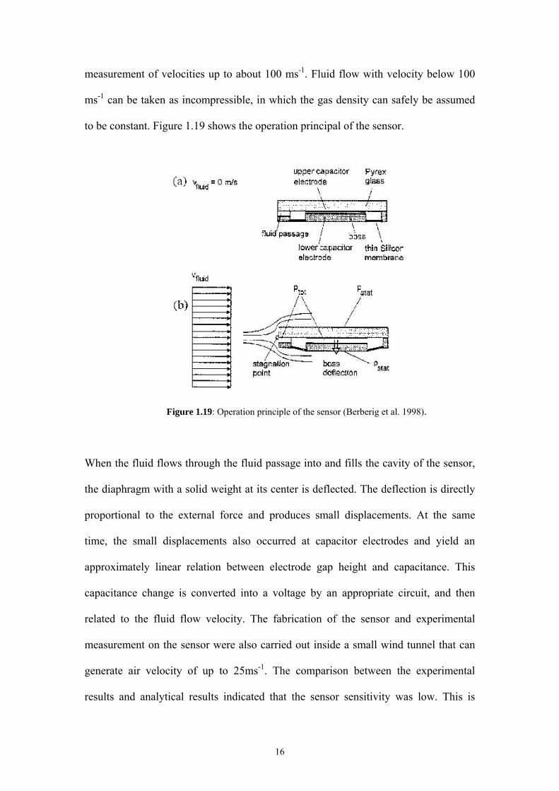
to be constant. Figure 1.19 shows the operation principal of the sensor.

Figure 1.19: Operation principle of the sensor (Berberig et al. 1998).

When the fluid flows through the fluid passage into and fills the cavity of the sensor,

the diaphragm with a solid weight at its center is deflected. The deflection is directly

proportional to the external force and produces small displacements. At the same

time, the small displacements also occurred at capacitor electrodes and yield an

approximately linear relation between electrode gap height and capacitance. This

capacitance change is converted into a voltage by an appropriate circuit, and then

related to the fluid flow velocity. The fabrication of the sensor and experimental

measurement on the sensor were also carried out inside a small wind tunnel that can

generate air velocity of up to 25ms-1. The comparison between the experimental

results and analytical results indicated that the sensor sensitivity was low. This is

17

because of the unfavorable ratio of Si wafer thickness (tSi=0.2mm) to Pyrex plate

thickness (tPy=1.2mm) which is causing significant reduction of the pressure inside

the PMFS (Prandtl Micro Flow Sensor) cavity. Figure 1.20 shows the comparison

results between experimental and analytical approach.

Figure 1.20: Readout signal as a function of flow velocity (Berberig et al. 1998).

In the electrochemical time of flight flow (TOF) sensor, the detection of

oxygen in the micro sensor is applied. This sensor design is made by Wu and Sansen

(2002). Figure 1.21 shows the cross section of the micro TOF flow sensor.

Figure 1.21: The cross section of the micro TOF flow sensor (both oxygen producer and oxygen sensor consist of a working electrode respectively. Only the working electrodes of both cells are shown for

simplicity) (Wu and Sansen, 2002).

18

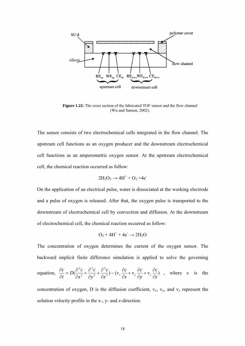
Figure 1.22: The cross section of the fabricated TOF sensor and the flow channel (Wu and Sansen, 2002).

The sensor consists of two electrochemical cells integrated in the flow channel. The

upstream cell functions as an oxygen producer and the downstream electrochemical

cell functions as an amperometric oxygen sensor. At the upstream electrochemical

cell, the chemical reaction occurred as follow:

2H2O2 → 4H+ + O2 +4e-

On the application of an electrical pulse, water is dissociated at the working electrode

and a pulse of oxygen is released. After that, the oxygen pulse is transported to the

downstream of electrochemical cell by convection and diffusion. At the downstream

of electrochemical cell, the chemical reaction occurred as follow:

O2 + 4H+ + 4e- → 2H2O

The concentration of oxygen determines the current of the oxygen sensor. The

backward implicit finite difference simulation is applied to solve the governing

equation, )()( 2

2

2

2

2

2

zcv

ycv

xcv

zc

yc

xcD

tc

zyx ∂∂

+∂∂

+∂∂

−∂∂

+∂∂

+∂∂

=∂∂ , where c is the

concentration of oxygen, D is the diffusion coefficient, vx, vy, and vz represent the

solution velocity profile in the x-, y- and z-direction.

19

Based on Figure 1.23, an oxygen pulse is produced at the upstream oxygen

producer and transported to the downstream by convection and diffusion. On the

passing of the oxygen pulses, peaks are formed on the current curves of the oxygen

sensor as shown in Figure 1.23(a). The breadth of the current peak depends on the

flow rate. Hence, the slower the flow rate, the wider the current peak. By observing

Figure 1.23(b), there is a good linearity between the reciprocal volume flow rates and

the positions of curve maxima.

Figure 1.23: The simulation of the oxygen sensor at the different flow rates. (a) The current vs. time curves; (b) the relationship between the flow rate and the position of the current maximum

(Wu and Sansen, 2002).

20

The experiment was also carried out and the corresponding results are shown in

Figure 1.24. Arrow ‘A’ points at the application of the electrical pulse on the

upstream cell, where the oxygen is produced. As already mentioned in the theoretical

part above, the passing of the oxygen pulse on the working electrode, distinct peak

forms on the current curve of the oxygen sensor. The experimental results also show

that the oxygen pulse is deformed and broadened by convection and diffusion during

the transportation. As the result, the positions of these peaks depend on the flow rates.

The study concluded that both digital simulation and measurement results show the

time difference between the production and detection of the oxygen pulse is only

related to the flow rate. The detection range of the sensor is between 1 and 15μl/min.

Figure 1.24: The current vs. time curves of the oxygen sensor at the different flow rates. Fluid: PBS. Flow rate: (a) 10μl/min; (b) 6μl/min; and (c) 4μl/min (Wu and Sansen, 2002).

21

Liu and Garimella (2003) have performed an investigation of liquid flow in

micro channels. Figures 1.25 and 1.26 shows the apparatus that was used to conduct

the experiment on the fluid flow in micro channel.

Figure 1.25: Schematic of the experimental apparatus (Liu and Garimella, 2003).

Figure 1.26: Schematic of the micro channel test section (Liu and Garimella, 2003).

After they conducted the experiment and analyzed the friction factor of the fluid flow

in micro channel, they found that the experimental results agree closely with the

theoretical predictions in the laminar region (see Figure 1.27). The experimental

results also show that the friction factors deviate from the laminar region when the

Reynolds number is approximately 3102× , which indicate the onset of transition. The

22

onset of transition of fluid flow for the micro channels are seen to agree with the

behavior in conventional channels.

Figure 1.27: Friction factor variation with Reynolds number in ‘long’ micro channels (Liu and Garimella, 2003).

When they analyzed the onset of transition in micro channel, they found that the

channel flow can stay laminar for Reynolds numbers of up to 50000 if completely

undisturbed. With the presence of perturbations, the onset of turbulence will occur at

3108.1Re ×= , below which the flow will remain laminar even with very strong

b)L3(Dh = 414μm)

23

disturbances. Results from the present work also suggest that no such early transition

occurs, at least down to hydraulic diameters of approximately 200μm. By observing

Figure 1.27, especially in Figure 1.27(b) and Figure 1.27(c) indicate that the transition

range extends up to Reynolds number of 4000. There are indications from Figure

1.27(a) that the flow becomes fully turbulent at 3105Re ×= . These values compare

favorably to 3103Re ×= , which is considered to be the minimum Reynolds number

for fully turbulent flow in conventional channels.

The examination on short micro channel had also been carried out in the experiment.

The experimental results showed that good agreement between experiment and

conventional correlations in the laminar regime, as shown in Figure 1.28.

Figure 1.28: Corrected friction factor variation with Reynolds number in ‘short’ micro channels (Liu and Garimella, 2003).

24

Figure 1.28: Corrected friction factor variation with Reynolds number in ‘short’ micro channels (cont’)

(Liu and Garimella, 2003).

Simulation by using a general – purposed finite volume – based computational fluid

dynamics (CFD) software package (FLUENT) have been carried out. The calculation

domain is shown in Figure 1.29. The results of the numerically predicted overall

pressure drop in the micro channels against the experimentally measured overall

pressure drop can be considered as satisfactory agreement, which are shown in Table

1.1.

Documents

3 – DIMENSIONAL COMPUTATIONAL ANALYSIS OF …eprints.usm.my/8922/1/3_–_DIMENSIONAL... · 1.5 Literature Reviews 6 CHAPTER 2: THEORY: COMPUTATIONAL SCHEME 2.1 Finite ... 1.50 Gauge