Embed Size (px)
Citation preview

1
Sanjeev Kumar JhaAssistant Professor
Earth and Environmental SciencesIndian Institute of Science Education and Research Bhopal
Email: [email protected]
Outline1.1. MotivationMotivation
FloodNet Project in CanadaFloodNet Project in Canada
Visits to the Canadian Flood Forecast Centres (FFCs)Visits to the Canadian Flood Forecast Centres (FFCs)
2.2. Identified Identified challenges/needs challenges/needs of the forecast centresof the forecast centres
3.3. Rainfall postRainfall post--processing (RPP) techniqueprocessing (RPP) technique
4.4. Application of RPP on the watersheds in Alberta and British ColumbiaApplication of RPP on the watersheds in Alberta and British Columbia
5.5. Ongoing development Ongoing development
2
FloodNet motivation
Floods are a major concern in Canada
Need for improved flood forecasting methods Need for improved flood forecasting methods
Opportunity for universities to work closely with flood forecast centres and conservation authorities
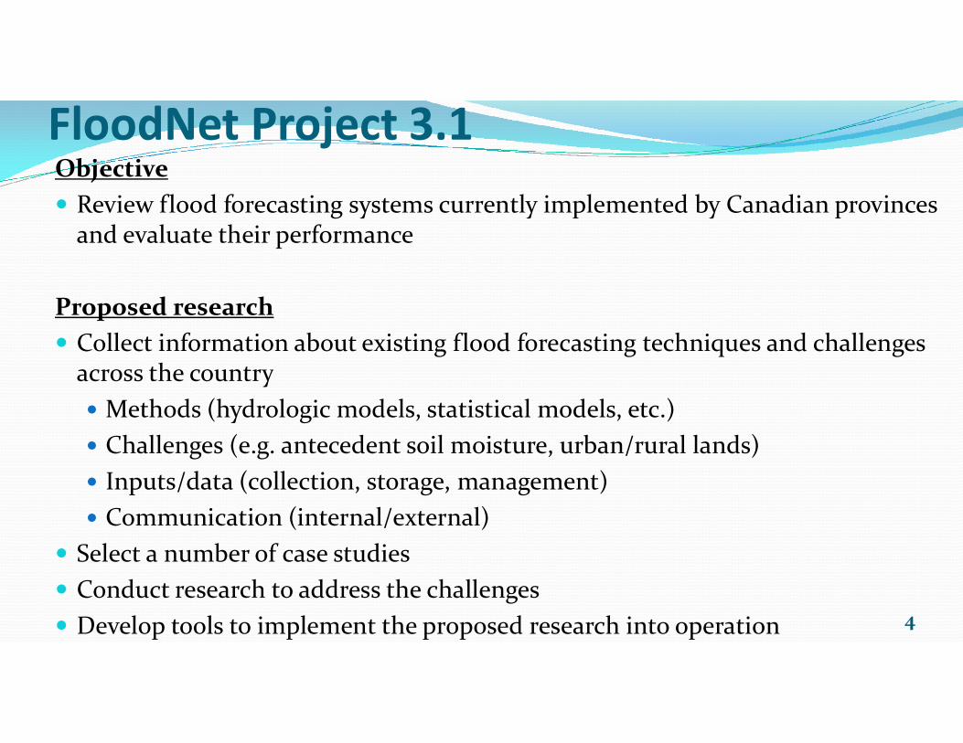
FloodNet Project 3.1Objective Review flood forecasting systems currently implemented by Canadian provinces
and evaluate their performance
Proposed research Collect information about existing flood forecasting techniques and challenges
across the countryacross the country Methods (hydrologic models, statistical models, etc.) Challenges (e.g. antecedent soil moisture, urban/rural lands) Inputs/data (collection, storage, management) Communication (internal/external)
Select a number of case studies Conduct research to address the challenges Develop tools to implement the proposed research into operation 4

Site visits
5
Ontario Ministry of Natural ResourcesSurface Water Monitoring System
CA’s:Toronto and Region Conservation Authority (TRCA)Credit Valley Conservation (CVC)

Research questions identified Data sources, collection and processing
Uncertainty in precipitation forecast obtained from Numerical Weather Prediction models The accuracy of streamflow forecast at upstream locations in neighbouring provinces or US states Determining antecedent soil moisture Estimating snow-water equivalent
Hydrologic and hydraulic modeling Hydrologic modelling of the Prairie region, characterized by a high percentage of non-contributing
areas due to potholes (western provinces) Presence of urban and rural areas in the same watershed (mostly eastern provinces) Consideration of regulated flow in hydrologic modelling Selection of the appropriate modelling system Need for an automated and integrated real-time forecast system
6
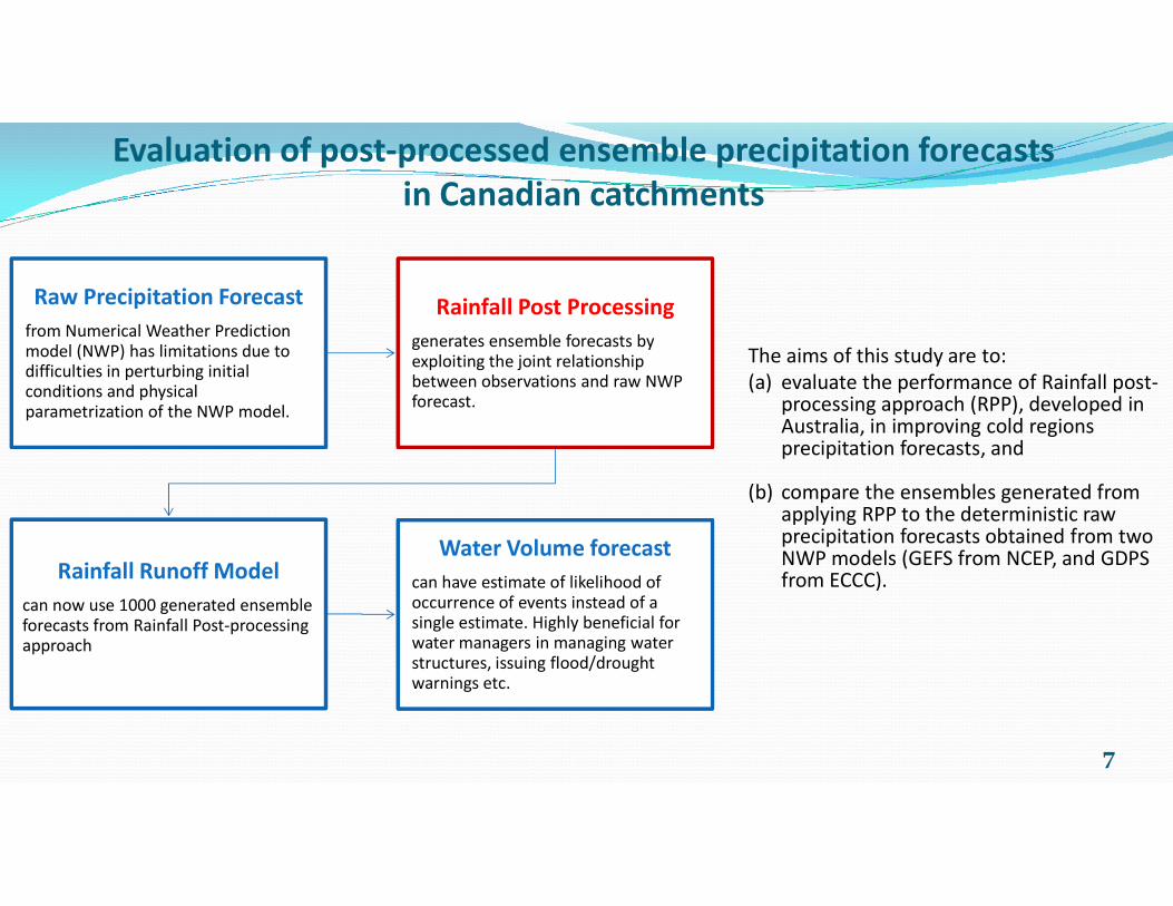
Raw Precipitation Forecastfrom Numerical Weather Prediction model (NWP) has limitations due to difficulties in perturbing initial conditions and physical parametrization of the NWP model.
Rainfall Post Processinggenerates ensemble forecasts by exploiting the joint relationship between observations and raw NWP forecast.
Evaluation of post-processed ensemble precipitation forecasts in Canadian catchments
The aims of this study are to: (a) evaluate the performance of Rainfall post-
processing approach (RPP), developed in Australia, in improving cold regions precipitation forecasts, and
7
Rainfall Runoff Modelcan now use 1000 generated ensemble forecasts from Rainfall Post-processing approach
Water Volume forecastcan have estimate of likelihood of occurrence of events instead of a single estimate. Highly beneficial for water managers in managing water structures, issuing flood/drought warnings etc.
precipitation forecasts, and
(b) compare the ensembles generated from applying RPP to the deterministic raw precipitation forecasts obtained from two NWP models (GEFS from NCEP, and GDPS from ECCC).
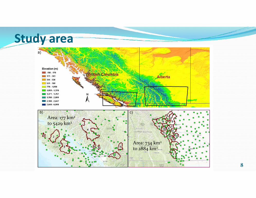
Study area
8
Area: 734 km2
to 2884 km2
Area: 177 km2
to 5429 km2
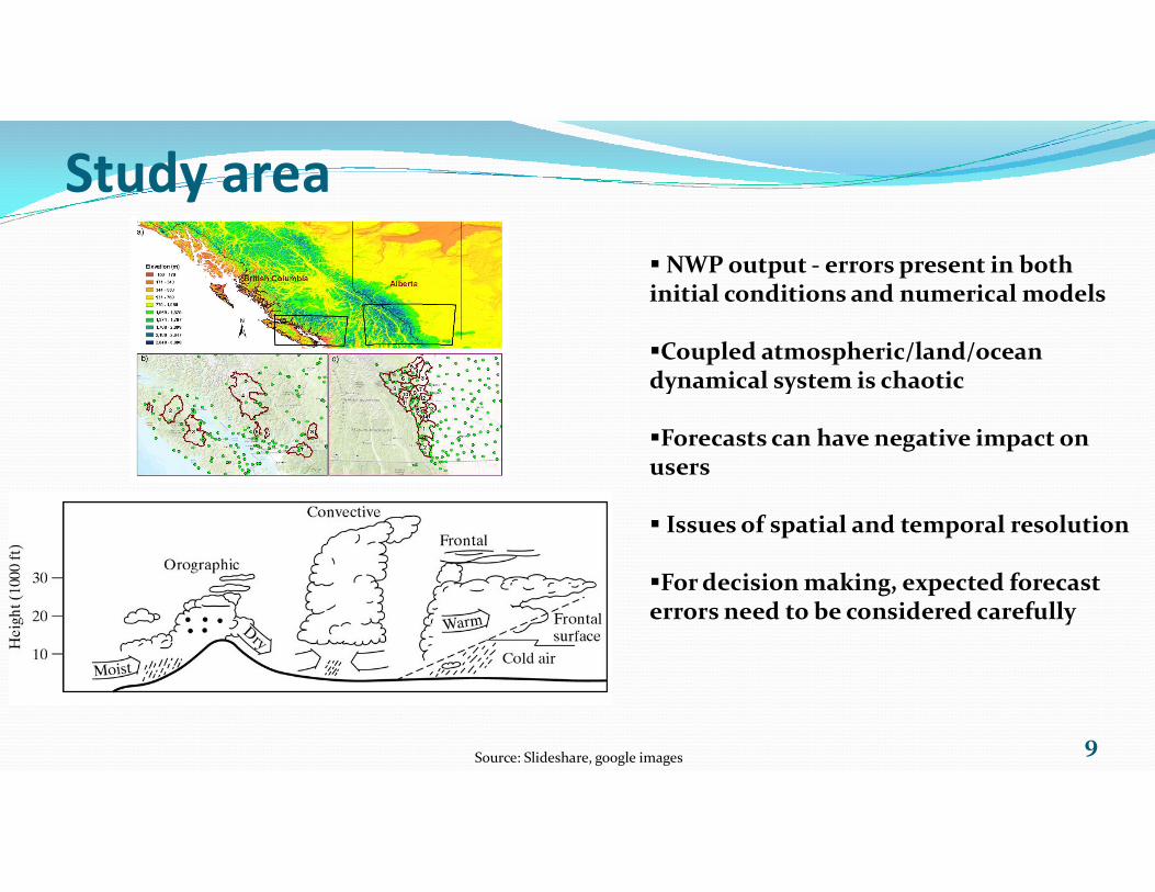
Study area NWP output - errors present in both initial conditions and numerical models
Coupled atmospheric/land/ocean dynamical system is chaotic
Forecasts can have negative impact on
9
Forecasts can have negative impact on users
Issues of spatial and temporal resolution
For decision making, expected forecast errors need to be considered carefully
Source: Slideshare, google images
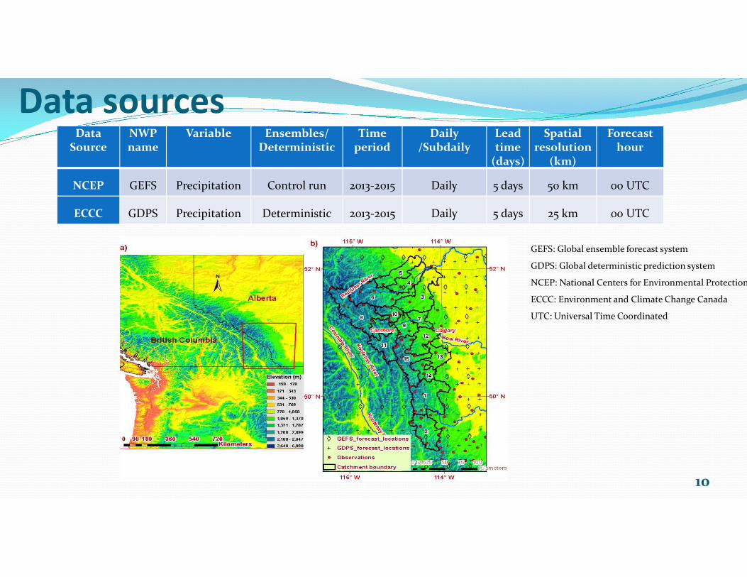
Data sourcesData
SourceNWP name
Variable Ensembles/Deterministic
Time period
Daily/Subdaily
Lead time
(days)
Spatial resolution
(km)
Forecast hour
NCEP GEFS Precipitation Control run 2013-2015 Daily 5 days 50 km 00 UTC
ECCC GDPS Precipitation Deterministic 2013-2015 Daily 5 days 25 km 00 UTC
GEFS: Global ensemble forecast system
GDPS: Global deterministic prediction system
NCEP: National Centers for Environmental Protection
10
ECCC: Environment and Climate Change Canada
UTC: Universal Time Coordinated
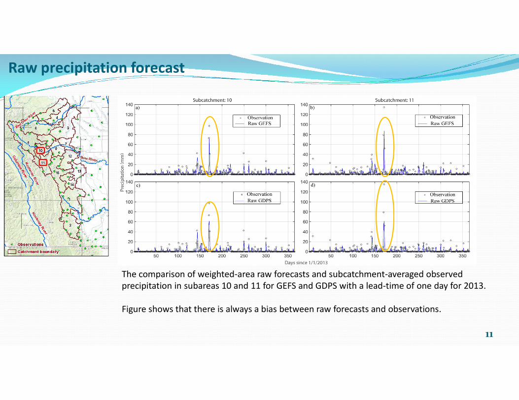
Raw precipitation forecast
11
The comparison of weighted-area raw forecasts and subcatchment-averaged observed precipitation in subareas 10 and 11 for GEFS and GDPS with a lead-time of one day for 2013.
Figure shows that there is always a bias between raw forecasts and observations.
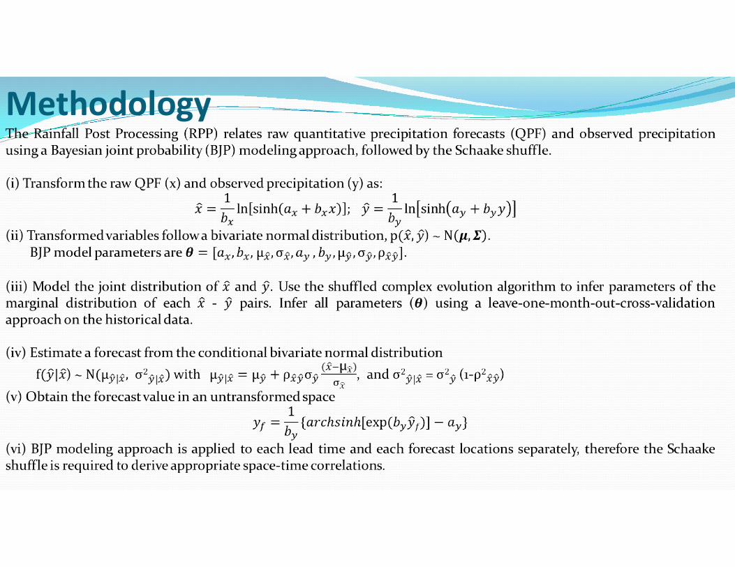
Methodology
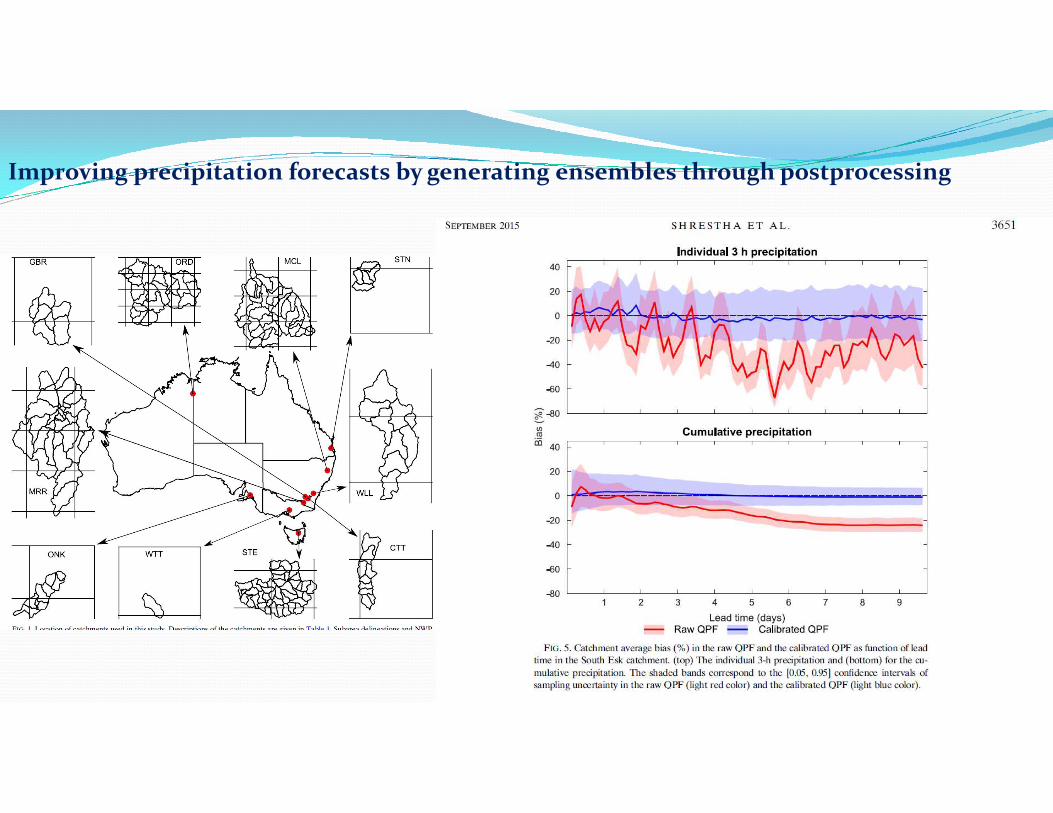
Improving precipitation forecasts by generating ensembles through postprocessing
13

Evaluation statistics
100
1
11
t
o
t
o
t
f
z
zz
Bias
Continuous rank probability score
t
of zzt
MAE1
1
Receiver operating characteristic
Hit
rate
False alarm rate
14
Spread-skill plotContinuous rank probability score
Source: pinimg.com; Nester et al. (2012), WRR; online presentation of Tom Hill, NOAA
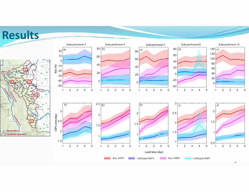
Results
15
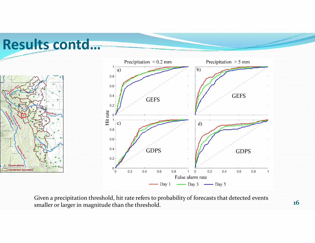
GEFSGEFS
Results contd…
16
GDPS GDPS
Given a precipitation threshold, hit rate refers to probability of forecasts that detected events smaller or larger in magnitude than the threshold.
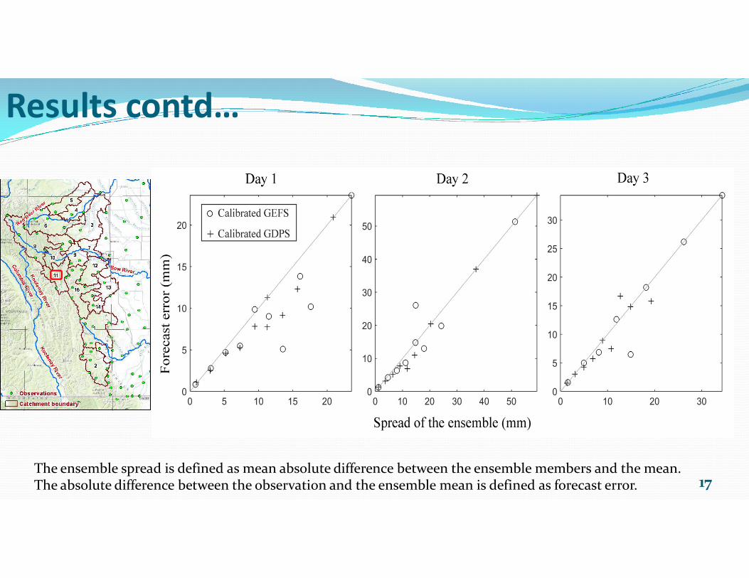
Results contd…
17The ensemble spread is defined as mean absolute difference between the ensemble members and the mean. The absolute difference between the observation and the ensemble mean is defined as forecast error.
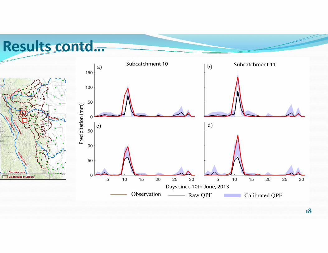
Results contd…
18
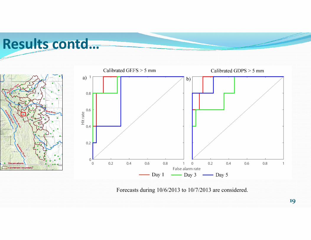
Results contd…
19
Forecasts during 10/6/2013 to 10/7/2013 are considered.
Conclusion:o Post-processed forecasts are demonstrated to have low bias, and higher accuracy for each lead-time in
15 subareas covering a range of topographical conditions from hills to plains.
o Post-processed forecast ensembles are able to capture peak precipitation events, which caused a major
flood event in the study area.
o Raw QPF need to be carefully examined before using in streamflow forecasting.
20
Ongoing work: o Apply RPP to other Canadian catchments under different climatic conditions
o Investigate into the influence of density of rain gauges
o Use a gridded reanalysis type data, e.g., CaPA as a substitute for observations.
o Uncertainty in streamflow forecasts using post-processed precipitation forecasts in a hydrologic model.
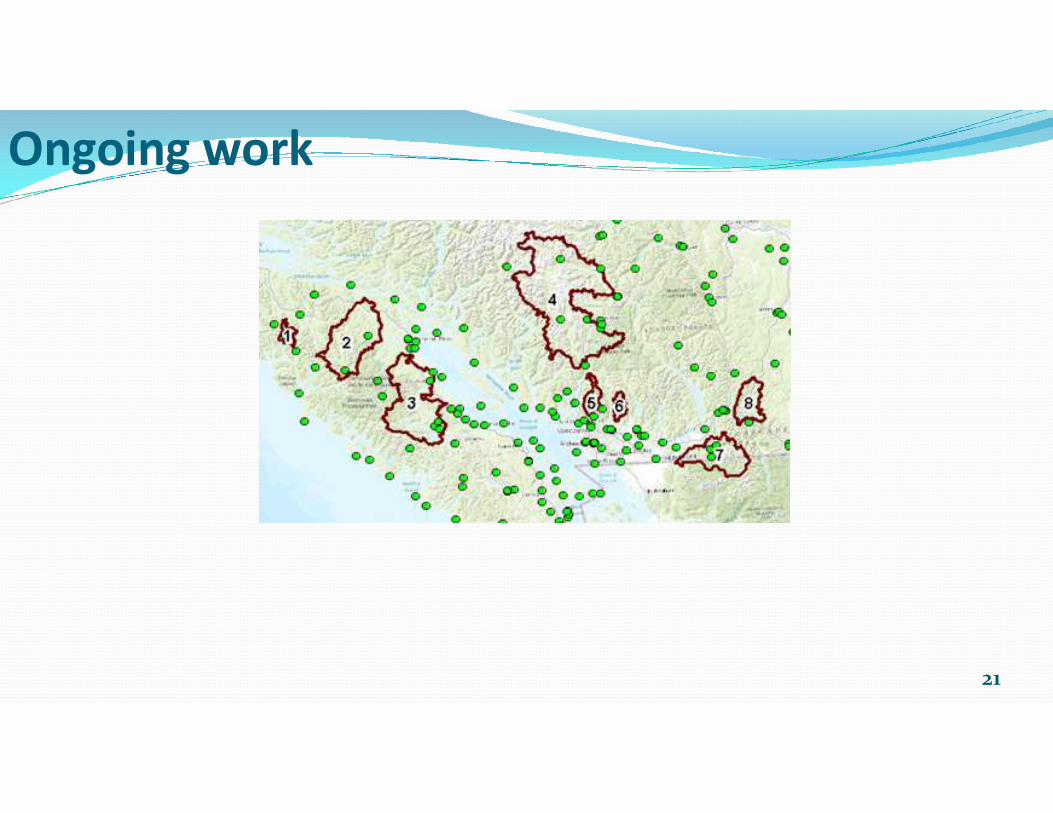
Ongoing work
21

Ongoing development at IISER Bhopal Development of SWAT model for river basins in MP NCMWRF agreed to share 35 km resolution NWP model output IIITM provided medium-range 100 km resolution NWP output
Observation data collected from MPWRD Observation data collected from MPWRD Gridded precipitation data from IMD
22

Acknowledgmentso Alberta and British Columbia River Forecast Centres provided rain gauge data and shape
files of catchments.
o Environment Canada provided GDPS forecast data
23
o Environment Canada provided GDPS forecast data
o CSIRO, Australia to share Rainfall Post-processing tool
o Dr. Gary Bates at NOAA – for his support related to GEFS data
o Late Dr. Peter Rasmussen – for leading FloodNet 3.1 project till January 2017
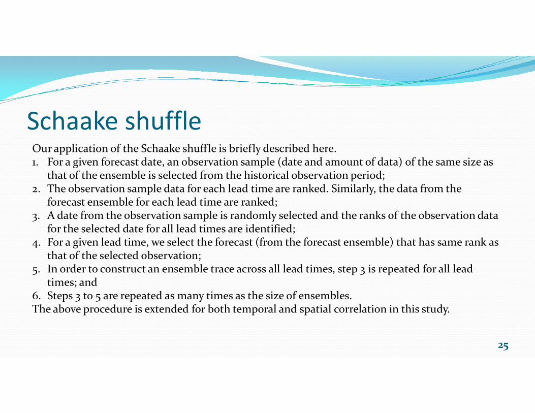
Schaake shuffleOur application of the Schaake shuffle is briefly described here.1. For a given forecast date, an observation sample (date and amount of data) of the same size as
that of the ensemble is selected from the historical observation period; 2. The observation sample data for each lead time are ranked. Similarly, the data from the
forecast ensemble for each lead time are ranked;
25
forecast ensemble for each lead time are ranked;3. A date from the observation sample is randomly selected and the ranks of the observation data
for the selected date for all lead times are identified; 4. For a given lead time, we select the forecast (from the forecast ensemble) that has same rank as
that of the selected observation;5. In order to construct an ensemble trace across all lead times, step 3 is repeated for all lead
times; and 6. Steps 3 to 5 are repeated as many times as the size of ensembles. The above procedure is extended for both temporal and spatial correlation in this study.