3. SEDIMAGING HARDWARE

This chapter describes the Sedimaging system hardware. The hardware consists of the

following subsystems as identified in Figure 3.1:

1. Sedimentation Column

2. Support Tower & Base

3. Positioning system

4. Pre-Segregation & Soil Release System

5. Connector & Drainage

6. Sediment Accumulator

7. Camera & Illumination

8. Computer & Monitor

Numbers shown in square brackets throughout this chapter refer to the labeled parts shown

in Figures 3.1 through 3.6. For brevity, further references to figure numbers are omitted

since the parts are easily located via the numbering scheme.

3.1 Sedimentation Column

The sedimentation column [1] is a 2.5 in. x 2.5 in. x 8 ft. aluminum square tube with 0.25

in. wall thickness. The sedimentation column is filled with water and the soil specimen is

introduced at its top. The particles settle down through this column and into the

accumulator below.

3.2 Support Tower & Base

The support tower [2] is a 4 in. x 6 in. x 6.5 ft. aluminum I-beam. The base [2] is a 1.5 ft. x

3.0 ft. x 0.5 in. aluminum plate. The support tower is bolted to the base. Together, they

provide resistance to overturning of the sedimentation column.

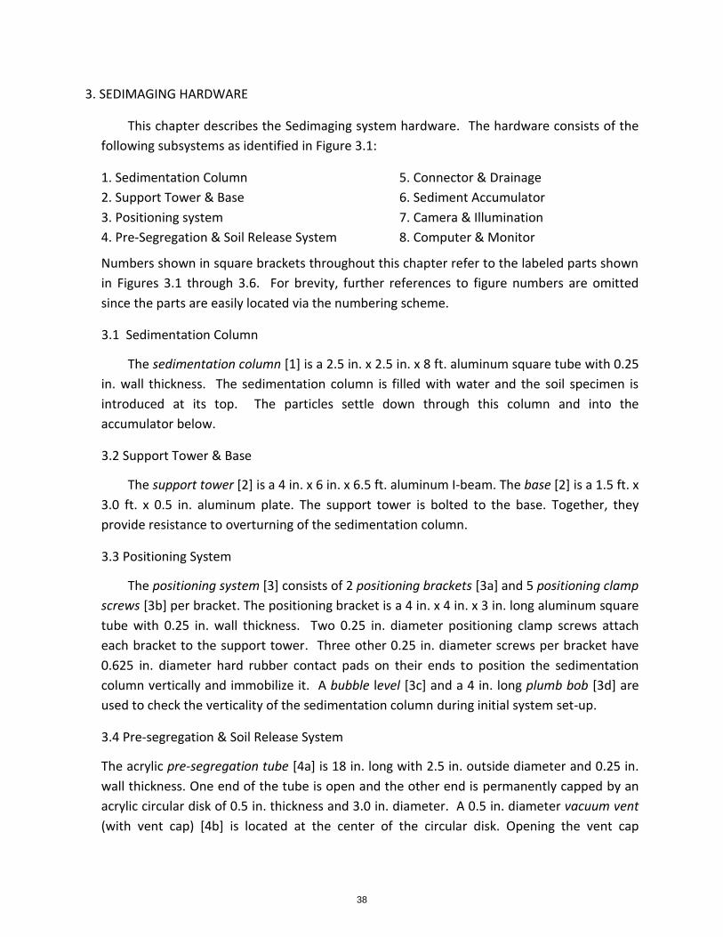
3.3 Positioning System

The positioning system [3] consists of 2 positioning brackets [3a] and 5 positioning clamp

screws [3b] per bracket. The positioning bracket is a 4 in. x 4 in. x 3 in. long aluminum square

tube with 0.25 in. wall thickness. Two 0.25 in. diameter positioning clamp screws attach

each bracket to the support tower. Three other 0.25 in. diameter screws per bracket have

0.625 in. diameter hard rubber contact pads on their ends to position the sedimentation

column vertically and immobilize it. A bubble level [3c] and a 4 in. long plumb bob [3d] are

used to check the verticality of the sedimentation column during initial system set-up.

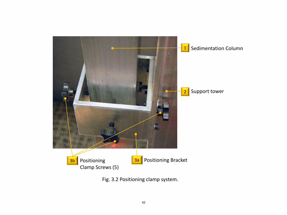
3.4 Pre-segregation & Soil Release System

The acrylic pre-segregation tube [4a] is 18 in. long with 2.5 in. outside diameter and 0.25 in.

wall thickness. One end of the tube is open and the other end is permanently capped by an

acrylic circular disk of 0.5 in. thickness and 3.0 in. diameter. A 0.5 in. diameter vacuum vent

(with vent cap) [4b] is located at the center of the circular disk. Opening the vent cap

38

releases the soil into the sedimentation column. Rubber membranes (party balloons with

snipped ends) [4c] are used to create a vacuum inside the pre-segregation tube as will be

explained in Chapter 6. A soil funnel [4d] with a 4 in. top diameter and a 0.7 in. spout

diameter assists with pouring of soil into the pre-segregation tube. A water container [4e]

fills the sedimentation column with 6000 mL of water. It also fills the pre-segregation tube

with about 1000 mL of water. The soil container [4f] is a 3.5 in. diameter x 2.0 in. high

aluminum canister. It is used to measure an appropriate volume of soil for transfer (through

the funnel) to the pre-segregation tube and subsequently for sedimentation.

A pre-segregation tube adaptor [4g] is also made of acrylic. It is circular on top and square

on the bottom. The pre-segregation tube adaptor mates the circular pre-segregation tube to

the square sedimentation column. The square part of the adaptor contains a 0.3 in.

diameter air vent on one side. It lines up with an identical hole in the sedimentation column.

This vent releases air from the sedimentation column allowing the introduction of the soil-

water mixture into the column. A 2.5 in. x 2.5 in. square gasket [4h] with a concentric 2.0 in.

diameter hole prevents water from escaping between the sedimentation column and the

pre-segregation tube adaptor. Similarly a round gasket [4i] with 2.5 in. outside diameter and

2.0 in. inside diameter is used to prevent leaks between the pre-segregation tube and the

pre-segregation tube adaptor.

3.5 Connector & Drainage

Located beneath the sedimentation column is a connector [5a] to the sediment accumulator

below. It consists of an outer 3 in. x 3 in. square tube with a 0.25 in. wall thickness and a 2.5

in. x 2.5 in. inner connector made from a square aluminum tube with 0.25 in. wall thickness.

Two 2.875 in. outside diameter x 0.09375 in. diameter rubber O-rings are positioned in

grooves inside the connector to prevent leaks between the sedimentation column and

connector and between the connector and the sediment accumulator. A drainage valve [5b]

with a socket cap screw for a valve stem has a 0.5 in. thread diameter and 1.75 in. length.

The valve stem passes through the connector and the 0.25 in. diameter tip of the stem is

flush with the inside wall of the connector when in the “closed” position. A 0.375 in. outside

diameter x 0.0625 in. diameter O-ring surrounds the drainage valve stem to prevent leaks

between the connector and the drainage valve when the valve is closed. When the drainage

valve is opened by unscrewing it, water is released from the system through a flexible 0.25 in.

inside diameter drainage tube [5c].

3.6 Sediment Accumulator

The sediment accumulator [6] consists of the sediment cartridge [6a], a cartridge pedestal

[6b], the cartridge support [6c], lower accumulator clamps [6d] and upper accumulator

39

clamps [6e]. The sediment cartridge [6a] is a 2.5 in. x 2.5 in. x 1 ft. long aluminum tube of

0.25 in. wall thickness. Two 10.25 in. x 2.0 in. x 0.125 in. borosilicate (Pyrex®) glass windows

are attached over openings on opposite sides of the sediment cartridge. The images of the

sedimented soils are taken through these windows. The largest soil particles which settle at

the very bottom of the sediment cartridge sit on top of the cartridge pedestal [6b] whose top

surface is 0.5 in. above the bottom of the windows to provide an unobstructed view of the

bottom of the sedimented soil column. The cartridge pedestal is milled down from a solid

square aluminum bar originally having 2.5 in. x 2.5 in. cross section and 2.25 in. length. The

pedestal is 2.0 in. x 2.0 in. in plan to fit precisely inside the sediment cartridge (above) and

inside the cartridge support (below). A 2.875 in. outside diameter x 0.09375 in. diameter O-

ring prevents leaks between the sediment cartridge and the cartridge pedestal. The pedestal

sits atop the 2.5 in. x 2.5 in. x 7.0 in. x 0.25 in. wall cartridge support [6c]. The two lower

accumulator clamps [6d] hold the sediment cartridge, the cartridge pedestal, and the

cartridge support together while the two upper accumulator clamps [6e] hold the

sedimentation column, connector, and the sediment cartridge together during a test.

3.7 Camera & Illumination

A 16.2 Mpix Nikon D7000 camera [7a] with and AF-S Micro NIKKOR 60 mm f/2.8G ED

Nikon lens [7b] are used to capture the images. A UC-E4 Nikon computer cable [7c] connects

the camera to a computer. An EH-5A Nikon AC power cord with EP-5 Nikon adaptor [7d]

provides AC power. A bi-directional bubble level [7e] is used to level the camera. A 4 in. x 6

in. x 1.5 ft. aluminum support column [7f] holds the camera and lighting. A camera bracket

[7g] is attached to the I-beam using 4 holding screws and the camera is attached to the

bracket using a single camera mounting screw. The 0.25 in. diameter camera holding screws

are used to adjust the camera in the x and y directions while the 0.25 in. diameter camera

mounting screw adjusts the camera in the y and z directions. The lighting [7h] is attached to

a light bracket [7i] fixed atop of the I-beam. The lighting removes shadows from the

sediment cartridge. A 6 in. engineering scale [7i] assists in precisely determining the camera

magnification.

3.8 Computer & Monitor

A microcomputer and monitor are used to control the camera and remotely capture

images using software NK Remote by Breeze Systems and then to analyze the image and

produce the grain size distribution curve through the computer program sedimaging.exe.

40

1

2

3

5

6

Sedimentation Column

Support Tower & Base

Positioning System

Connector & Drainage

Sediment Accumulator

7 Camera & Illumination

8 Computer & Monitor

4 Pre-segregation & Soil Release System (not shown in this figure)

Fig. 3.1 Sedimaging system overview photographs. 41

3a Positioning Bracket 3b Positioning Clamp Screws (5)

1

2

Sedimentation Column

Support tower

Fig. 3.2 Positioning clamp system.

42

6

4g 4a

4h Round Gasket

5 Connector & Drain Pre-segregation Tube Adaptor

Pre-segregation Tube

Sediment Accumulator Plumb Bob

Soil Funnel

Water Container

Soil Container

Rubber Membranes (party balloons)

Level

Engineering Scale

4i Square Gasket

4c

4f

4e

3c

7i

4d

3d

Fig. 3.3 Various sedimaging system parts and accessories. 43

Pre-segregation Tube

Vacuum vent

Pre-segregation Tube Adaptor

exploded view

4b

4a

4g

Fig. 3.4 Pre-segregation and soil release system.

44

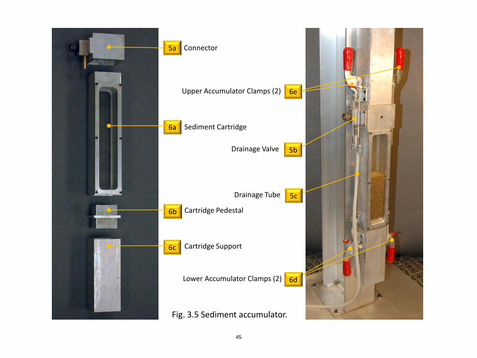
5a

6a

Connector

Sediment Cartridge

6b Cartridge Pedestal

6c Cartridge Support

Lower Accumulator Clamps (2)

Upper Accumulator Clamps (2)

Drainage Valve

Drainage Tube

6d

6e

5b

5c

Fig. 3.5 Sediment accumulator.

45

Nikon D7000 Camera

Lighting

Camera Support Column

7h

7a

7f

Nikor AF-S 60 mm Lens 7b

Bi-directional Bubble Level 7e

AC Power Cord w/ Adaptor 7d

Computer Cable 7c

Camera Bracket 7g

Light Bracket 7i

Fig. 3.6 Camera and illumination system.

46

4. SEDIMAGING SOFTWARE

4.1 NKRemote

NKRemote by Breeze Systems ($175) (http://www.breezesys.com/index.htm) facilitates remote control of Nikon digital SLR cameras from a microcomputer. It is ideally suited for Sedimaging as several of the program’s features are utilized including:

a) Live view on a computer monitor of the scene in the camera’s field of view.

b) Full control of all camera settings from the computer.

c) Digital zooming on a zone of interest in the field of view.

d) Remote manual focusing on a zone of interest, or on the full image.

e) Remote image capture and direct file storage to the computer hard drive.

4.2 Sedimaging.exe

Sedimaging.exe is an executable program that was developed at the University

of Michigan using MATLAB by Mathworks. MATLAB is a high-level computer

language that performs many mathematical tasks, particularly those involving matrix

algebra, faster than traditional programming languages such as Fortran and C++.

The Sedimaging program crops the image taken by NKRemote, performs the image

processing and outputs the test results with minimal user interaction. Since

Sedimaging.exe is a compiled executable program, the user does not use MATLAB

directly and will not need to have it installed on the Sedimaging system’s

microcomputer.

47

5. SEDIMAGING SYSTEM SET-UP

5.1 System Location

The sedimaging system’s current design requires 10 ft. clearance to permit installation

of the pre-segregation tube above the sedimentation column. To attach the pre-

segregation system, a ladder with a platform 5 ft. above the ground may be used, although

any system deemed appropriate by the user may be used. The base should be located on as

even a surface as possible. A leveling bubble should be used to find the permanent location.

Shims may be used if necessary. However, shims can slip and re-leveling may be necessary.

It is best to quasi-permanently affix the base using floor bolts to avoid having to re-level

after initial installation.

5.2 Camera System Installation

a. The required distance between the surface of the camera lens and the outside surface

of the sediment accumulator window is 12.7 in. This distance is based on the 23.6

mm x 15.6 mm sensor size of the D7000 camera, the 60 mm camera focal length, and

the nominal 5 in. required height of the sedimented soil column.

b. Attach the camera bracket to the camera support column using four 0.25 in. diameter

screws and nuts. These screws adjust the camera position in the plane parallel to the

surface of the sediment accumulator window.

c. Attach the camera to the camera bracket using a 0.25 in. diameter camera mounting

screw. The distance between the camera and soil accumulator can be adjusted over a

range of 2.2 in. by choosing different mounting holes on the bracket. Choose the hole

that provides as closely as possible the required 12.7 in. camera lens to accumulator

window distance.

d. Insert the EP-5 Nikon adaptor into the battery compartment of the camera and

connect the EH-5A Nikon AC power adaptor. Connect the adaptor to a laboratory

power source.

e. Connect the UC-E4 Nikon camera-to-computer cable to the camera’s micro-USB

socket. The socket can be found under a rubber panel of the D7000. Connect the

other end of the cable to a free USB port on the computer.

f. Level the camera using the bi-directional bubble level so that the surface of the

camera lens is vertical. If the camera is not vertical adjust it using the camera

mounting screw.

48

5.3 Sedimaging System Alignment

a. Use the bubble level and plumb bob to establish sedimentation column verticality.

The plumb bob can be lowered on its string through the center of the sedimentation

column. A top cap fits snugly into the top of the sedimentation column to position

the string at dead center. The plumb bob should be lowered to within a few

millimeters of the accumulator pedestal. Adjust the column location using the

positioning clamp screws which are attached to the positioning bracket until column

verticality is achieved. This happens when the plumb bob is directly above the center

mark on the pedestal. Check with the bubble level placed on the outside of the

column.

Advanced Problems and Troubleshooting: Disagreement between plumb bob and

bubble level occurs only if the soil accumulator is not evenly clamped to the

sedimentation column. A long straight edge with a cut-out for the connector can be

used to see if the outside surfaces of the column and accumulator are parallel. If

they are not, consider replacing the O-rings. Another possibility is that the clamping

compressive forces are uneven on the two sides. The user can check this by “feel”

when clamping down on both sides simultaneously. If this happens, and O-Rings are

not worn, try rotating the accumulator 180 degrees. If the compression forces flip

sides the nuts on the clamping rods require adjustment.

b. Set the exposure mode of the camera to manual by turning the mode dial to < M >.

Set the camera to autofocus by setting the AF mode switch to < AF >.

c. Open < NKRemote > and adjust camera settings to the following (Figure 5.1 Step 1):

Shutter speed (Tv) < 1/10 >

Aperture size (Av) < 3.2 >

Sensitivity (ISO) < 100 >

Exposure compensation < none >

Image quality < JPEG Normal >

Image size < Large 4928x3264 >

White balance < Auto >

Metering mode < Matrix >

Picture control < Standard >

Autofocus mode < Single >

Check the center focus point box from 39 focus point boxes.

49

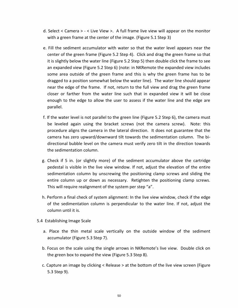
d. Select < Camera > - < Live View >. A full frame live view will appear on the monitor

with a green frame at the center of the image. (Figure 5.1 Step 3)

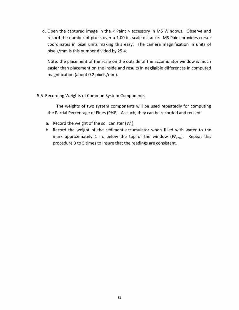
e. Fill the sediment accumulator with water so that the water level appears near the

center of the green frame (Figure 5.2 Step 4). Click and drag the green frame so that

it is slightly below the water line (Figure 5.2 Step 5) then double click the frame to see

an expanded view (Figure 5.2 Step 6) (note: in NKRemote the expanded view includes

some area outside of the green frame and this is why the green frame has to be

dragged to a position somewhat below the water line). The water line should appear

near the edge of the frame. If not, return to the full view and drag the green frame

closer or farther from the water line such that in expanded view it will be close

enough to the edge to allow the user to assess if the water line and the edge are

parallel.

f. If the water level is not parallel to the green line (Figure 5.2 Step 6), the camera must

be leveled again using the bracket screws (not the camera screw). Note: this

procedure aligns the camera in the lateral direction. It does not guarantee that the

camera has zero upward/downward tilt towards the sedimentation column. The bi-

directional bubble level on the camera must verify zero tilt in the direction towards

the sedimentation column.

g. Check if 5 in. (or slightly more) of the sediment accumulator above the cartridge

pedestal is visible in the live view window. If not, adjust the elevation of the entire

sedimentation column by unscrewing the positioning clamp screws and sliding the

entire column up or down as necessary. Retighten the positioning clamp screws.

This will require realignment of the system per step “a”.

h. Perform a final check of system alignment: In the live view window, check if the edge

of the sedimentation column is perpendicular to the water line. If not, adjust the

column until it is.

5.4 Establishing Image Scale

a. Place the thin metal scale vertically on the outside window of the sediment

accumulator (Figure 5.3 Step 7).

b. Focus on the scale using the single arrows in NKRemote’s live view. Double click on

the green box to expand the view (Figure 5.3 Step 8).

c. Capture an image by clicking < Release > at the bottom of the live view screen (Figure

5.3 Step 9).

50

d. Open the captured image in the < Paint > accessory in MS Windows. Observe and

record the number of pixels over a 1.00 in. scale distance. MS Paint provides cursor

coordinates in pixel units making this easy. The camera magnification in units of

pixels/mm is this number divided by 25.4.

Note: the placement of the scale on the outside of the accumulator window is much

easier than placement on the inside and results in negligible differences in computed

magnification (about 0.2 pixels/mm).

5.5 Recording Weights of Common System Components

The weights of two system components will be used repeatedly for computing

the Partial Percentage of Fines (P%F). As such, they can be recorded and reused:

a. Record the weight of the soil canister (Wc)

b. Record the weight of the sediment accumulator when filled with water to the

mark approximately 1 in. below the top of the window (Wa+w). Repeat this

procedure 3 to 5 times to insure that the readings are consistent.

51

1 3

1

3

Inputting the camera settings from NKRemote’s main window.

Live view window will pop-up showing the sediment accumulator.

Fig. 5.1 Inputting the camera settings and opening the live view window.

2

2 Opening the live view window.

52

Fig. 5.2 Leveling the sedimentation column using a water level in the sediment accumulator.

4

5

6

Filling the sediment accumulator with water to about the center of the green frame.

Fine-tuning the focus using the single arrow keys and checking camera alignment relative to the water level.

6

Moving the green box below the water level by clicking & draging then double clicking the box to expand the view.

5 4

53

7 8

9 Fig. 5.3 Determining image magnification using a scale on the sediment accumulator window.

7

8

9

Putting a scale on the sediment accumulator.

Fine-tuning the focus using the single arrow keys from the zoomed view of the scale.

Captured image of the sediment accumulator with a scale.

54

6. SEDIMAGING TEST PROCEDURE

This chapter assumes that the soil specimen contains only particles smaller than 2 mm

(100% passing a #10 sieve). For soils containing particles larger than 2 mm please refer to

procedures in Section 12. To determine the percentage of fines, the weight of the soil

canister (Wc) and the weight of the sediment accumulator filled with water (Wa+w) should

have been determined per instructions in Section 5.5. Sections 6.1 through 6.14, are all

associated with correspondingly numbered figures.

6.1 Soil and Sedimentation Column Preparation

1) Fill the soil canister with a dry specimen. For soils with a typical specific gravity (Gs) of

2.65 this will be approximately 450 g +/- 25 g.

2) Weigh and record the weight of soil (Ws = Ws+c – Wc).

3) Fill the sedimentation column with 6000 mL of water.

6.2 Assembling the Pre-segregation Tube Adaptor

4) Place the square gasket on top of the sedimentation column

5) Slide the pre-segregation tube adaptor onto the sedimentation column making sure

that the vent holes in the adaptor and sedimentation column line up.

6) Lower the circular gasket into the adaptor

6.3 Placing Water and Soil into the Pre-Segregation Tube

7) Fill the pre-segregation tube with water until about half full and using the funnel pour

the soil specimen into the tube.

8) Add additional water to the pre-segregation tube to the fill mark on the tube.

6.4 Installing the Rubber Membrane on the Pre-Segregation Tube

9) Stretch a rubber membrane over the open end of the tube.

10) Push the membrane into the tube while lifting one edge of the membrane so that a

vacuum remains in the tube once the membrane snaps back onto the tube.

11) Insure that a vacuum has been created by observing a concave surface in the

membrane. The center of the membrane should be approximately 0.5 in. below the

end of the tube. If 0.5 in. concavity has not been achieved try again.

6.5 Soil Pre-Segregation

12) Invert the pre-segregation tube containing the soil and water mixture several times

until the particles are well mixed then turn vertically with the membrane on the

bottom.

13) Hold the tube vertically with the membrane on the bottom for several seconds

allowing the coarser particles to settle down. At this point, an optional step may be

55

added to remove excessive fines from the specimen. If the pre-segregation tube is

inverted such that the open end is on top, the membrane can be removed and the

dirty water can be syphoned or syringed from the tube (a turkey baster is

recommended). The removed dirty water should be released over a #20 sieve to

recover and return particles larger than 0.075 mm to the pre-segregation tube. In a

related case, if a specimen contains small amounts of very low specific gravity

particles such as organic debris, mica flakes or chips of shale rock, they should be

permanently removed. Otherwise these objects would come to rest within the

matrix of finer particles and the image processing would interpret the soil as being

somewhat coarser than by sieving.

14) Roll the membrane off of the end of the tube.

15) Removal of the membrane creates an upward seepage gradient through the soil which

will prevent the soil from slipping out of the tube.

6.6 Soil Release into the Sedimentation Column

16) Lower the pre-segregation tube into the adaptor.

17) Remove the vent cap from the top of the pre-segregation tube.

18) The soil-water mixture immediately drops into the sedimentation column. Air from

the top of the sedimentation column escapes through small holes in the side of the

sedimentation column and adaptor.

6.7 Draining the Sedimentation Column

19) Once approximately 3 to 4 mm of particles smaller than 0.075 mm have settled in the

accumulator (this takes 5 to 10 minutes depending on the specimen particle sizes and

gradation), open the drainage valve to allow water to drain completely from the

column. The drainage can begin sooner if it is obvious that the entire soil specimen

has settled in the accumulator.

20) Complete drainage of the water (with fines) from the sedimentation column will occur

in approximately 3 minutes. As just mentioned, some fines will have entered into

the accumulator prior to opening the drainage valve. This is desirable for accurate

determination of the percentage of fines in the specimen. The imaging will account

for the fines that have settled in the accumulator.

6.8 Tapping the Column

21-23) After drainage ends, tap the accumulator sharply once so that the top surface of

the soil becomes perfectly flat. A ¼ in. Allen wrench is suggested for the task.

6.9 Focusing and Capturing an Image

56

24) Open the program NKRemote and select <Camera> then <Live view>. The live image

appears with a green rectangular frame at the center of the image.

25) Double-click the area in the green frame. This expands the view of this area for closer

inspection. Using the single arrows at the bottom of the screen will fine- tune the

focus. Double clicking the image returns the full view. By clicking on a different part

of the image other areas can be expanded and similarly inspected. If the camera and

sedimentation column are properly aligned, all areas should be in focus after fine-

tuning the focus on the center area. A lack of focus in other areas is an indication

that either the camera or the sedimentation column or both are out of alignment and

need to be realigned per instructions in Chapter 5.

26) Take an image of the soil column by pressing the <Release> button and immediately

move to the next step.

6.10 Detaching Connector and Accumulator, Removing Water with Fines

27) Release the sediment accumulator from the sedimentation column by pulling down on

the two upper accumulator clamps.

28) Lower and remove the detached connector and accumulator assembly.

29) Using a large syringe (e.g. a turkey baster), remove all but about 3 inches of the dirty

water from above the sedimented soil. Keep the syringe well above the soil

surface and fill it slowly enough so as to not remove fines that settled prior to

image capture. Steps 27 through 29 should be performed as rapidly as possible.

Theoretically, all fines that had not settled prior to image capture should be

removed during this step.

6.11 Refilling with Clean Water, Removing Connector and Weighing

30) Using the syringe, refill the accumulator with clean water to the same level as was

used to determine Wwf+a (Section 5.5).

31) The water fill mark is indicated by the horizontal etched lines on the accumulator

window frame.

32) Detach the connector & drainage valve from the column.

33) Weigh the sediment accumulator containing soil and water (Ws+wf+a).

Determine the partial percentage of fines (P%F) by:

P%F = (Ws -Wsa)/Ws x 100(%)

where

Wsa = Gs[Ws+wf+a – Wa+w]/(Gs – 1)

For most silica sands, Gs is in the range between 2.64 and 2.69 in which case Wsa

may be approximated by:

57

Wsa = 1.6[Ws+wf+a – Wa+w]

For the required 450 +/- 25 g soil specimen the error in P%F will be less than

0.5% by this approximation. However, use of a known Gs is always preferred.

Note: the term “partial percentage of fines” is used because other fines have

settled in the accumulator and were photographed. The fines in the

accumulator are accounted for by the image processing software. The

Sedimaging program combines the two fines components to yield the total

percentage of fines.

6.12 Inputing Soil and Image Information into the Sedimaging Computer Program

34) Place the captured image file in the folder that contains the Sedimaging program <

Sedimaging.exe >. Then open <Sedimaging.exe >. Dialog boxes will appear.

35) Enter a soil name, file name, magnification, Ws+c and Ws+wf+a. Press “OK” after each

entry.

36) Enter the requested background data for the specimen.

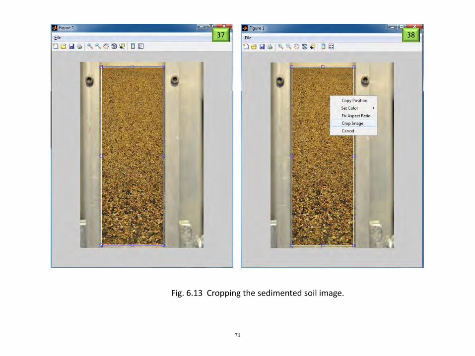
6.13 Cropping the Sedimented Soil Image

37) After pressing the last “OK” the sedimented soil image will appear. Click to create a

cropping box. Adjust the box by stretching the little blue squares located on the

edges of the box to encompass the soil area. Avoid cropping the image outside of the

soil area.

38) Right-click and select “Crop Image”.

6.14 Viewing, Saving and Printing Sedimaging Results

39) After cropping, the test results will automatically appear. Print and/or save the image

as a jpg file.

6.15 Printing Results in Tabular Form

40) Percents passing standard sieves are presented in tabular form.

6.16 Cleaning the System

Empty the sediment accumulator then rinse it and the pre-segregation tube, pre-

segregation tube adaptor, and rubber gaskets. Occasional rinsing the sedimentation

column interior is also recommended to remove leftover fines from interior walls.

The lower sediment accumulator clamps do not need to be opened except for very

occasional cleaning. The tolerances are small enough that only very fine sands could

fall into the gap between the window and pedestal. If they do, it will be visually

apparent that a cleaning is necessary.

58

1

3

2

Filling the soil canister with a representative specimen of the soil.

Weighing the soil & canister.

1

2

3 Filling the sedimentation column with 6000 mL of water.

Fig. 6.1 Soil and sedimentation column preparation.

59

4

6

5

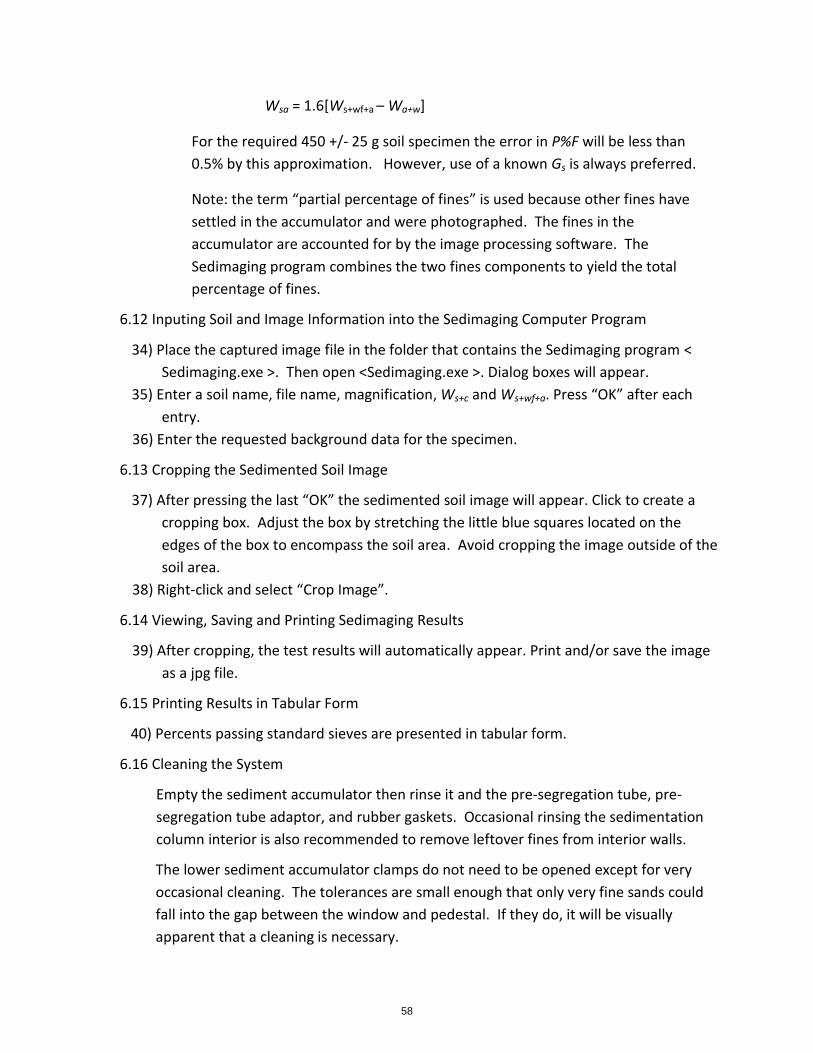
Laying square gasket on top of the the sedimentation column.

Sliding pre-segregation tube adaptor onto the sedimentation column.

4

5

6 Lowering the circular gasket into the adaptor.

Fig. 6.2 Assembling the pre-segregation tube adaptor.

60

7 8

Pouring soil through funnel into the pre-segregation tube about half pre-filled with water.

7 8 Filling tube with water up to mark.

Fig. 6.3 Placing water and soil into the pre-segregation tube.

61

9

10

11

Fig. 6.4 Installing the rubber membrane on the pre-segregation tube.

9

10

11

Stretching rubber membrane over open end of pre-segregation tube.

Pressing rubber membrane into tube while allowing air to escape.

Vacuum in tube results in membrane concavity.

62

12 13 14

15 Fig. 6.5 Soil pre-segregation.

12

13

14

Rotating pre-segregation tube 180 degrees several times

and shaking to mix soil very well in the water.

Allowing coarse-grained fraction of the sediment to Settle to the membrane-capped end of the tube.

Slipping the membrane off.

15 Saturated soil will not slip out of the tube because of the vacuum.

63

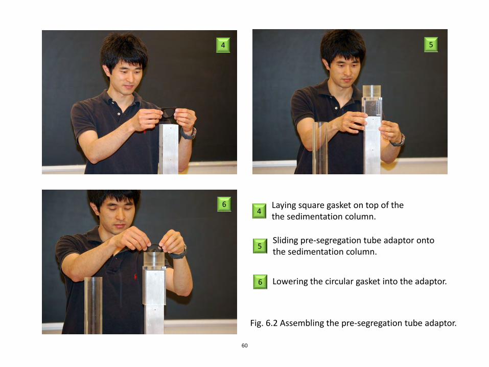
16 17 18

Fig. 6.6 Soil release into sedimentation column.

16

17

18

Pre-segregation tube with soil placed in adaptor.

Opening vent releases soil into the sedimentation column.

Soil-water mixture enters column in 1 to 2 seconds.

64

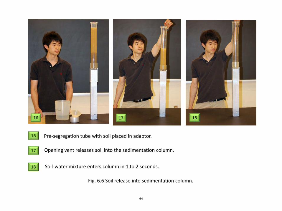
Fig. 6.7 Draining the sedimentation column

19

20

Opening drainage valve.

Emptying through drainage line.

19

20

65

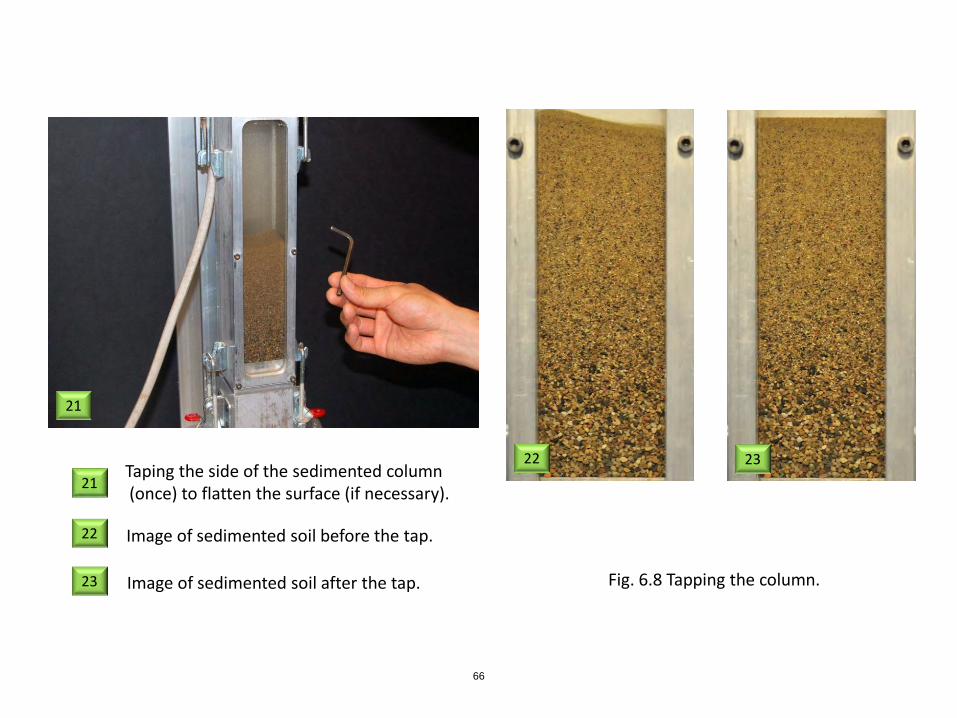
Fig. 6.8 Tapping the column.

21

21

22

23

Taping the side of the sedimented column (once) to flatten the surface (if necessary).

Image of sedimented soil before the tap.

22 23

Image of sedimented soil after the tap.

66

24 25

26 Fig. 6.9 Focusing and capturing an image.

24

25

26

Selecting an area to zoom in on.

Fine-tuning the focus using the single arrow keys.

Returning to full view to capture an image.

67

Fig. 6.10 Detaching connector and accumulator, removing water with fines

27 Releasing the clamps.

28 Detaching the connector & accumulator.

27

28

29 Removing some dirty water.

29

68

Fig. 6.11 Refilling with clean water, removing connector and weighing.

33

Lifting and removing the connector.

Refilling with clean water to the mark on the accumulator.

30

31

32

33

30

32

31

Weighing the accumulator with soil and water.

&

69

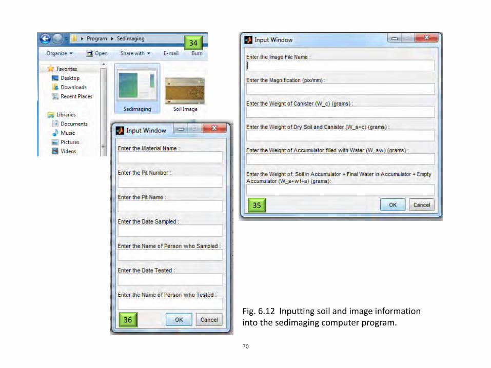
34

35

36 Fig. 6.12 Inputting soil and image information into the sedimaging computer program.

70

37 38

Fig. 6.13 Cropping the sedimented soil image.

71

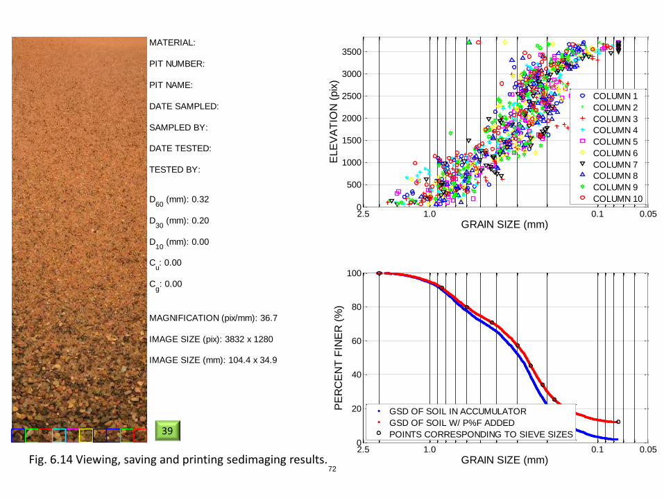
MATERIAL:

PIT NUMBER:

PIT NAME:

DATE SAMPLED:

SAMPLED BY:

DATE TESTED:

TESTED BY:

D60

(mm): 0.32

D30

(mm): 0.20

D10

(mm): 0.00

Cu: 0.00

Cg: 0.00

MAGNIFICATION (pix/mm): 36.7

IMAGE SIZE (pix): 3832 x 1280

IMAGE SIZE (mm): 104.4 x 34.9

0.050.11.02.50

500

1000

1500

2000

2500

3000

3500

GRAIN SIZE (mm)

ELE

VA

TIO

N (

pix

)

COLUMN 1

COLUMN 2

COLUMN 3

COLUMN 4

COLUMN 5

COLUMN 6

COLUMN 7

COLUMN 8

COLUMN 9

COLUMN 10

0.050.11.02.50

20

40

60

80

100

GRAIN SIZE (mm)

PE

RC

EN

T F

INE

R (

%)

GSD OF SOIL IN ACCUMULATOR

GSD OF SOIL W/ P%F ADDED

POINTS CORRESPONDING TO SIEVE SIZES

Fig. 6.14 Viewing, saving and printing sedimaging results.

39

72

Fig. 6.15 Printing results in tabular form.

40

73

7. TRANSLUCENT SEGREGATION TABLE (TST) THEORETICAL CONCEPTS

7.1 Thresholding and Binary Image Creation

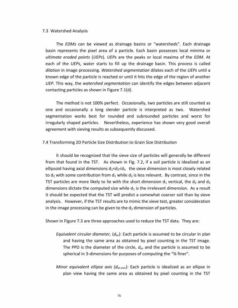
If the pixels representing each particle in an image can be counted the grain size

distribution can easily be determined. In order to count the number of pixels in each

particle, the particles need to be separated from the background by assigning

different pixel values to the particles than to the background. This is accomplished by

first converting the original 8-bit RGB color image to a gray scale image then

converting the gray scale image to a binary image. The RGB color image has three

color channels (red, green and blue) and each color has 256 shades ranging from 0 to

255. The grayscale image has 256 shades of gray from pure black to pure white. By

contrast, a binary image has only two pixel values; black (0) and white (1). The RGB

color image is converted to the grayscale image using the formula gray = (red + green

+ blue) / 3. Then, the grayscale image is converted to the binary image using a

threshold value. If the pixel value of the grayscale image is smaller than the threshold

value, the pixel value will be replaced by 0. On the other hand, if the pixel value of the

grayscale image is larger than the threshold value, the pixel value becomes 1. Figure

7.1(b) shows a binary image created from a section of a TST image, Figure 7.1(a).

The threshold value can be set manually or set automatically by the ImageJ

program. Because the translucent segregation table has very bright illumination

coming from five 24 in fluorescent light bulbs in the light box beneath the translucent

plate, the grayscale value of particle pixels is close to black (0) and the grayscale value

of the background is nearly white (255) as was observed in Figure 7.1(a). This allows

ImageJ to automatically convert the grayscale image to the binary image without

setting the threshold value manually.

7.2 Euclidian Distance Map

The translucent segregation table does not prevent the particles from being in

contact with each other; it only prevents small particles from hiding behind large

particles by segregating them somewhat and, with user assistance, arranging them in

a single layer. Separating the contacting particles is called segmentation in image

processing and the segmentation method that ImageJ uses is watershed segmentation

from a Euclidian distance map (EDM).

The EDM is generated by replacing each foreground (particle) pixel with a pixel

value equal to that pixel’s distance from the nearest background (light table) pixel.

74

7.3 Watershed Analysis

The EDMs can be viewed as drainage basins or “watersheds”. Each drainage

basin represents the pixel area of a particle. Each basin possesses local minima or

ultimate eroded points (UEPs). UEPs are the peaks or local maxima of the EDM. At

each of the UEPs, water starts to fill up the drainage basin. This process is called

dilation in image processing. Watershed segmentation dilates each of the UEPs until a

known edge of the particle is reached or until it hits the edge of the region of another

UEP. This way, the watershed segmentation can identify the edges between adjacent

contacting particles as shown in Figure 7.1(d).

The method is not 100% perfect. Occasionally, two particles are still counted as

one and occasionally a long slender particle is interpreted as two. Watershed

segmentation works best for rounded and subrounded particles and worst for

irregularly shaped particles. Nevertheless, experience has shown very good overall

agreement with sieving results as subsequently discussed.

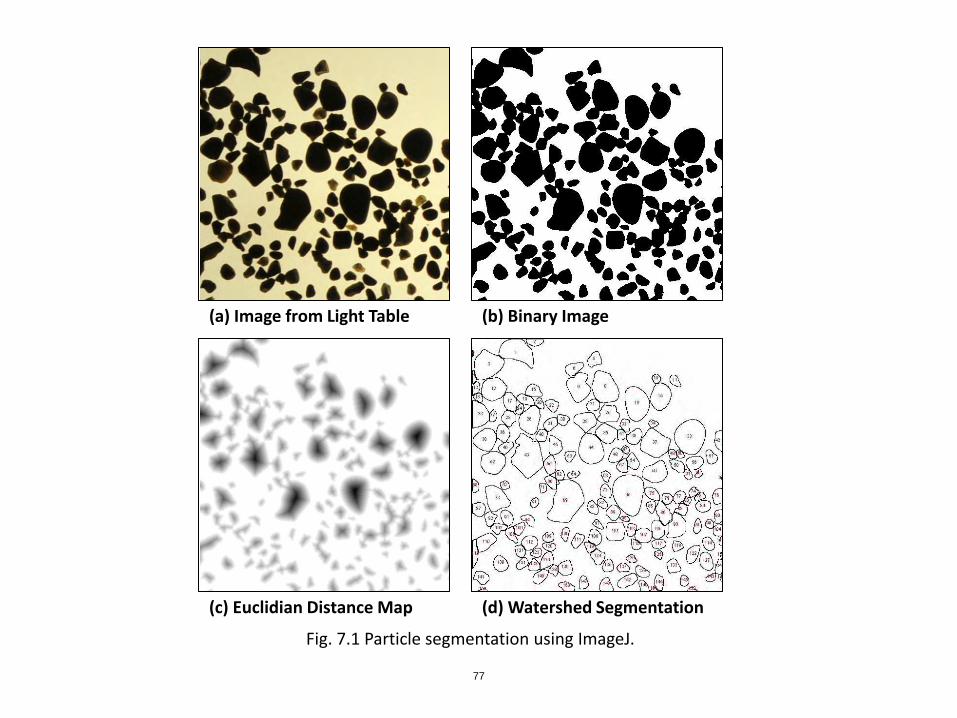
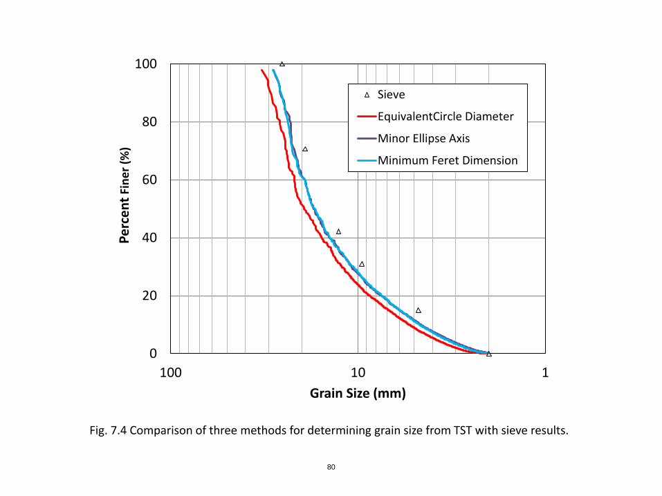
7.4 Transforming 2D Particle Size Distribution to Grain Size Distribution

It should be recognized that the sieve size of particles will generally be different

from that found in the TST. As shown in Fig. 7.2, if a soil particle is idealized as an

ellipsoid having axial dimensions d1<d2<d3 the sieve dimension is most closely related

to d2 with some contribution from d1 while d3 is less relevant. By contrast, since in the

TST particles are more likely to lie with the short dimension d1 vertical, the d2 and d3

dimensions dictate the computed size while d1 is the irrelevant dimension. As a result

it should be expected that the TST will predict a somewhat coarser soil than by sieve

analysis. However, if the TST results are to mimic the sieve test, greater consideration

in the image processing can be given to the d2 dimension of particles.

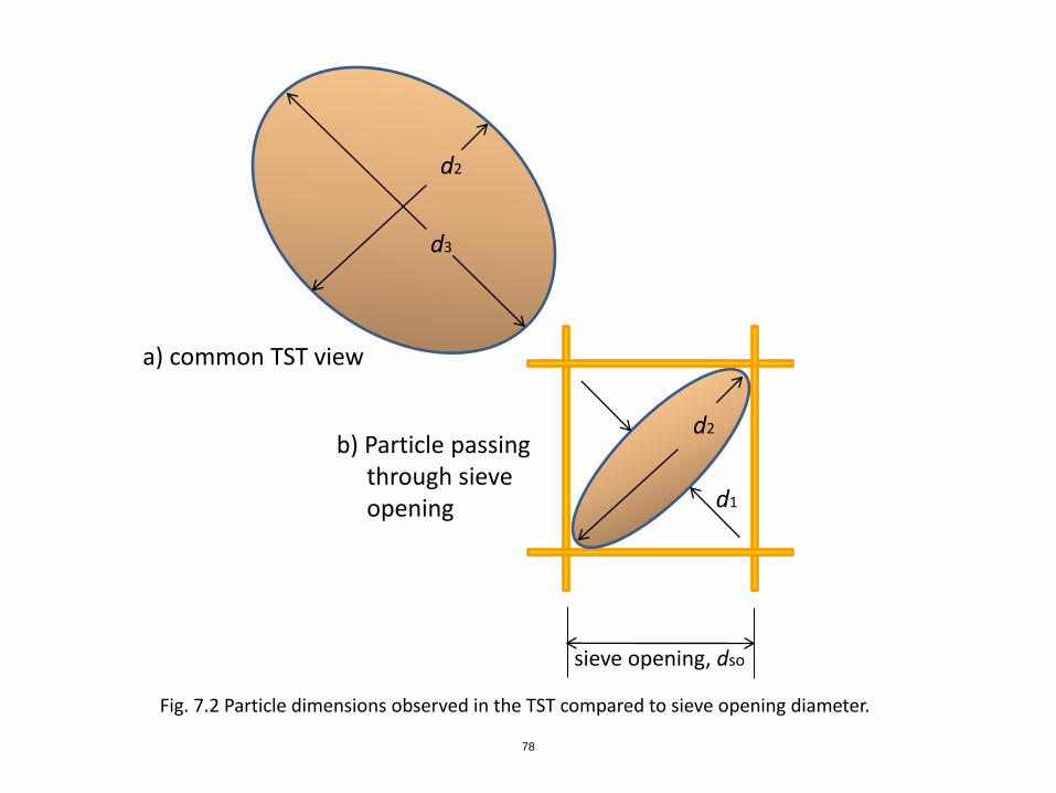
Shown in Figure 7.3 are three approaches used to reduce the TST data. They are:

Equivalent circular diameter, (dec): Each particle is assumed to be circular in plan

and having the same area as obtained by pixel counting in the TST image.

The PPD is the diameter of the circle, dec and the particle is assumed to be

spherical in 3-dimensions for purposes of computing the “% finer”.

Minor equivalent ellipse axis (del-min): Each particle is idealized as an ellipse in

plan view having the same area as obtained by pixel counting in the TST

75

image. To fit each particle with an ellipse the centroid of the ellipse is made

to coincide with centroid of the particle. The PPD is assumed to be del-min.

To compute the “% finer” the volume may be assumed proportional to

del-min3, or better, proportional to (del-min

2)( del-max).

Minimum feret dimension (df-min) the minimum feret dimension can be thought

of as the smallest caliper distance or the shortest distance between two

parallel lines both tangent to the particle on opposite sides. The PPD is

assumed to be df-min. To compute the “% finer” the volume may be assumed

proportional to df-min 3, or better, proportional to (df-min

2)( df-max).

In both the minor equivalent ellipse axis method and the minimum feret dimension

method the vertical dimension (d1) is assumed to be equal to the smaller plan view

dimension, del-min or df-min for purposes of computing particle volumes.

Fig. 7.4 compares sieve test results with TST results using the three methods described

above. As expected, the equivalent circle method yields the coarsest grain size curve

and is least similar to sieve results. The minor equivalent ellipse axis method and the

minimum feret dimension method yield virtually identical results and are much more

similar to sieve results. Finally, Figure 7.5 shows that a slight improvement is achieved

by using (del-min 2)( del-max) rather than del-min

3 to compute soil particle volumes for “%

finer”. As such, this method is presently recommended for use with the TST.

However, it is also recommended that in future testing the bridge underpass heights

be utilized to estimate d1 thereby allowing all three particle dimensions to be used for

computing particle volumes.

Note: Referring to Fig. 7.2, for a very flat disk-like particles (d1 approaching zero) the

difference between the sieve-based grain size and the TST-based PPD is a factor of √2

= 1.4. For perfect spheres, the sieve results and the TST methods should produce

identical results. As such, the grain size curves will always be offset by a factor

between 1.0 and about 1.4 with the former value expected for very rounded particles

and the latter expected for very flat particles. The curves in Fig. 7.5 are offset by a

factor of 1.2.

The TST.exe program discussed in Chapter 11 prints the results by both the equivalent

circular diameter method and by the minor equivalent ellipse axis method. The

difference between the two curves serves as an indication of the particle aspect ratios.

76

(a) Image from Light Table (b) Binary Image

(c) Euclidian Distance Map (d) Watershed Segmentation

Fig. 7.1 Particle segmentation using ImageJ. 77

sieve opening, dso

d3

d2

d1

d2

a) common TST view

Fig. 7.2 Particle dimensions observed in the TST compared to sieve opening diameter.

b) Particle passing through sieve opening

78

dec . c

del-min

del-max

df-min

a) Diameter of equivalent area circle

b) Minimum and maximum dimensions of equivalent area ellipse

c) Minimum ferret dimension.

Fig. 7.3 Definitions of particle diameter.

79

0

20

40

60

80

100

110100

Pe

rce

nt

Fin

er

(%)

Grain Size (mm)

Sieve

EquivalentCircle Diameter

Minor Ellipse Axis

Minimum Feret Dimension

Fig. 7.4 Comparison of three methods for determining grain size from TST with sieve results.

80

0

20

40

60

80

100

110100

Pe

rce

nt

Fin

er

(%)

Grain Size (mm)

Sieve

(Minor Ellipse Axis)^3

(Minor Ellipse Axis)^2 x (Major EllipseAxis)

Fig. 7.5 Comparison of TST results using only d2 versus using d2 and d3 for computing particle volume.

81

8. TST HARDWARE

The Translucent Segregation Table (TST) hardware can be grouped into four subsystems as shown in the photographs in Figure 8.1:

1. Camera System; 2. Computer and Monitor;

3. Translucent Segregation Table; 4. Ancillary Supplies

Bracketed numbers in this chapter refer to the parts labeled in Figures 8.1 to 8.6.

8.1 Camera System

The camera system [1] consists of a 16.2 Mpixel Nikon D7000 [1a], an AF-S Micro

NIKKOR 60 mm f/2.8G ED lens [1b], a bi-directional bubble level [1c], an EH-5A Nikon AC

power cord with EP-5 Nikon adaptor [1d], the UC-E4 Nikon camera-to-computer cable [1e], a

camera bracket [1f] and a ceiling bracket [1g]. The camera bracket is made from 2

aluminum pieces of dimensions 2 in. x 3 in. x 0.5 in. and 5 in. x 3 in. x 0.5 in.. The first piece

of the camera bracket is attached to the ceiling bracket with four 0.25 in. diameter screws

while the second piece of the camera bracket holds the camera with another 0.25 in.

diameter screw. The holding screw location can be adjusted to achieve different camera

magnifications as dictated by the ceiling height. The ceiling bracket is a 3 in. x 24 in. x 0.5 in.

aluminum bar which drop-mounts into a conventional drop ceiling panel.

8.2 Computer and Monitor

A microcomputer and monitor are used to control the camera and capture images remotely

through NK Remote software. The computer analyzes the images and determines the grain

size distribution by ImageJ and MATLAB software.

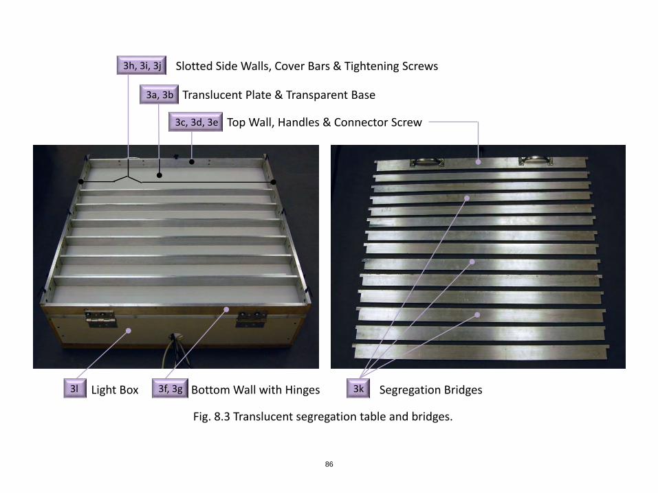
8.3 Translucent Segregation Table (TST)

The Translucent Segregation Table is the heart of the system. Its main component is a

36 in. x 36 in. x 0.375 in. square translucent plate [3a] made of white acrylic which is fixed to

a 36 in. x 36 in. x 0.5 in. transparent base [3b]. The translucent plate acts as a diffuser for

the light coming from below. It provides a bright and uniform background for the soil image.

Scratches on this translucent surface do not appear in the images. The transparent base is

attached to the underside of the translucent plate to stiffen the plate system. By increasing

the plate rigidity displacements of the translucent plate caused by self-weight and the

weight of soil are minimized. A 35 in. x 2 in. x 0.5 in. top wall [3c] has two 5.7 in. handles

[3d] for lifting and inclining the plate assembly. By removing a 3 in. x 0.25 in. diameter

connector screw [3e], the top plate can be lifted out to allow sweeping out the soil after

testing. The connector screw extends from the top of the top wall to the transparent base

and provides additional support to the plate system. A 35 in. x 2 in. x 0.5 in. aluminum

82

bottom wall [3f] is permanently attached to the translucent plate, the translucent base and

slotted side walls. Two 4 in. x 2 in. hinges [3g] connect the bottom wall to the light box and

allow the translucent plate, with all walls and bridges, to incline while still connected to the

light box. Two 36 in. x 2 in. x 0.5 in. slotted aluminum side walls [3h] are permanently fixed

to the lateral sides of the TST plate. They contain 18 0.375 in. x 0.5 in. x 0.5 in. matched

slots for the bridges. Only some of the slots are used in any one test, but the large number

of available slots provides great flexibility to achieve more uniform particle distribution.

The TST system comes with 13 interchangeable segregation bridges [3k] each being 36 in. x

0.375 in. x various heights. The different bridges provide different underpass heights, the

equivalent of sieve opening sizes. The two bridge ends slide into the slotted side walls in

various bridge combinations and spacings as deemed suitable for a particular specimen.

Two prismatic square 0.5 in. x 0.5 in. x 36 in. cover bars [3i] sit on top of the side walls and

immobilize the segregation bridges using tightening screws [3j]. With a quarter turn, two of

the tightening screws on each side release the cover bar entirely while the third screw on

each side allows the cover bar to pivot out from the slotted side walls. This allows for bridge

placement or removal.

Two 23 in. long L-channels serve as support feet [3m] for the inclined translucent plate

assembly. During system transport, the two support feet are attached to the two side walls

using two 0.25 in. threaded immobilizing screws [3n]. Two 0.5 in. pivot screws and nuts [3o]

on the other end of the L-channels allow the support feet to rotate down into a vertical

position for particle segregation. As a safety measure against accidental kick-out of the

feet, the immobilizing screws are installed into threaded holes at the base of the light box.

The light box [3l] is a 36 in. x 36 in. x 7 in. particle board frame. It houses five 24 in.

fluorescent lights [3p]. A 7 in. high translucent acrylic support column [3q] stands at the

center of the light box to provide additional support to the translucent plate assembly when

the plate is in the lowered position.

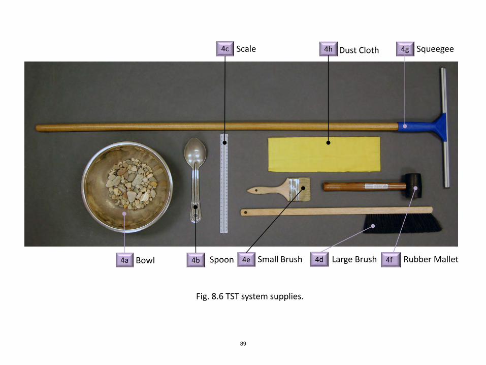
8.4 Ancillary Supplies

A number of ancillary items assist in the performance of the TST test. They include a

large bowl [4a] and spoon [4b] used to prepare soil and place it on the translucent plate. An

engineering scale [4c] is used to determine the camera magnification. A large brush [4d]

loosens soil clogs behind the segregation bridges and distributes soil evenly along the length

of the bridges. A small brush [4e] performs the same task for smaller particles. A rubber

mallet [4f] is employed to tap the corner of the light table after segregation to spread the

soil particles into a single layer. A squeegee [4g] removes soil from the light table and a dust

cloth (4h) wipes the translucent plate surface after a test.

83

1

2

3

Camera System

Computer & Monitor

Translucent Segregation Table

4 Ancillary Supplies (not shown)

Fig. 8.1 Translucent Segregation Table (TST) system overview. 84

Nikon D7000 Camera

1a

Nikor AF-S 60 mm Lens

1b

Bi-directional Bubble Level

1c

Power Adaptor 1d

Computer Cable 1e

Camera Bracket 1f

Ceiling Bracket 1g

Fig. 8.2 TST camera system.

85

3a, 3b

Segregation Bridges 3l

3c, 3d, 3e

3f, 3g

3h, 3i, 3j

3k

Translucent Plate & Transparent Base

Light Box

Top Wall, Handles & Connector Screw

Bottom Wall with Hinges

Slotted Side Walls, Cover Bars & Tightening Screws

Fig. 8.3 Translucent segregation table and bridges.

86

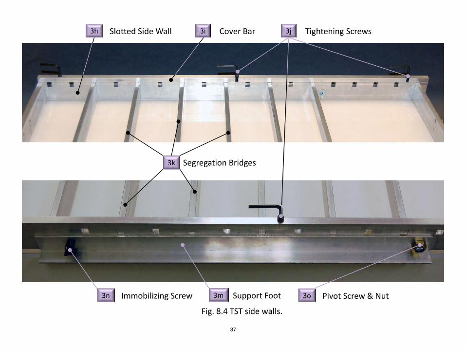
3h Slotted Side Wall 3i Cover Bar 3j Tightening Screws

Segregation Bridges 3k

3m Support Foot 3n Immobilizing Screw 3o Pivot Screw & Nut

Fig. 8.4 TST side walls.

87

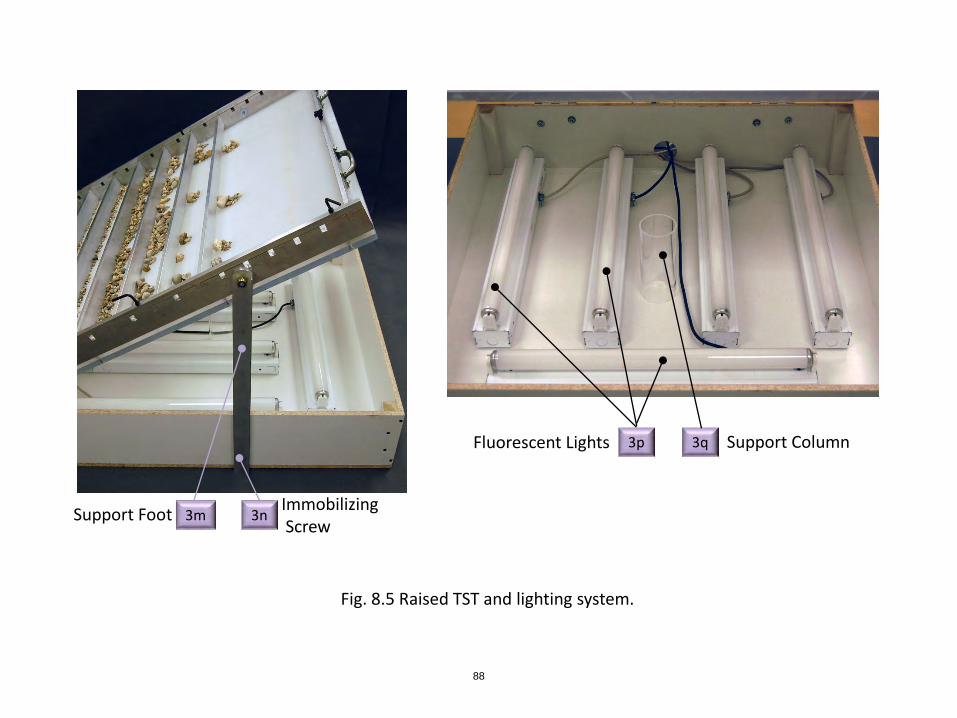
3m Support Foot 3n Immobilizing Screw

3p Fluorescent Lights 3q Support Column

Fig. 8.5 Raised TST and lighting system.

88

4a 4b

4c

4d 4e 4f

4h 4g

Bowl Spoon Large Brush

Scale

Small Brush Rubber Mallet

Squeegee Dust Cloth

Fig. 8.6 TST system supplies.

89