Embed Size (px)
Citation preview

3,350+OPEN ACCESS BOOKS
108,000+INTERNATIONAL
AUTHORS AND EDITORS115+ MILLION
DOWNLOADS
BOOKSDELIVERED TO
151 COUNTRIES
AUTHORS AMONG
TOP 1%MOST CITED SCIENTIST
12.2%AUTHORS AND EDITORS
FROM TOP 500 UNIVERSITIES
Selection of our books indexed in theBook Citation Index in Web of Science™
Core Collection (BKCI)
Chapter from the book Industrial Robotics : Theory, Modelling and ControlDownloaded from:http://www.intechopen.com/books/industrial_robotics_theory_modelling_and_control
PUBLISHED BY
World's largest Science,Technology & Medicine
Open Access book publisher
Interested in publishing with IntechOpen?Contact us at [email protected]

237
8
A Complete Family of Kinematically-Simple Joint Layouts: Layout Models, Associated Displacement
Problem Solutions and Applications
Scott Nokleby and Ron Podhorodeski
1. Introduction
Podhorodeski and Pittens (1992, 1994) and Podhorodeski (1992) defined a ki-nematically-simple (KS) layout as a manipulator layout that incorporates a spherical group of joints at the wrist with a main-arm comprised of success-fully parallel or perpendicular joints with no unnecessary offsets or link lengths between joints. Having a spherical group of joints within the layouts ensures, as demonstrated by Pieper (1968), that a closed-form solution for the inverse displacement problem exists. Using the notation of possible joint axes directions shown in Figure 1 and ar-guments of kinematic equivalency and mobility of the layouts, Podhorodeski and Pittens (1992, 1994) showed that there are only five unique, revolute-only, main-arm joint layouts representative of all layouts belonging to the KS family. These layouts have joint directions CBE, CAE, BCE, BEF, and AEF and are de-noted KS 1 to 5 in Figure 2.
Figure 1. Possible Joint Directions for the KS Family of Layouts
Source: Industrial-Robotics-Theory-Modelling-Control, ISBN 3-86611-285-8, pp. 964, ARS/plV, Germany, December 2006, Edited by: Sam Cubero
Ope
n A
cces
s D
atab
ase
ww
w.i-
tech
onlin
e.co
m
238 Industrial Robotics: Theory, Modelling and Control
KS 1 - CBE KS 2 - CAE
KS 3 - BCE
KS 4 - BEF
KS 5 - AEF
KS 6 - CCE
KS 7 - BBE
KS 8 - CED
KS 9 - ACE
KS 10 - ACF
KS 11 - CFD
KS 12 - BCF
KS 13 - CED
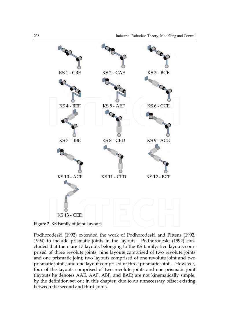
Figure 2. KS Family of Joint Layouts
Podhorodeski (1992) extended the work of Podhorodeski and Pittens (1992, 1994) to include prismatic joints in the layouts. Podhorodeski (1992) con-cluded that there are 17 layouts belonging to the KS family: five layouts com-prised of three revolute joints; nine layouts comprised of two revolute joints and one prismatic joint; two layouts comprised of one revolute joint and two prismatic joints; and one layout comprised of three prismatic joints. However, four of the layouts comprised of two revolute joints and one prismatic joint (layouts he denotes AAE, AAF, ABF, and BAE) are not kinematically simple, by the definition set out in this chapter, due to an unnecessary offset existing between the second and third joints.

A Complete Family of Kinematically-Simple Joint Layouts: Layout Models… 239
Yang et al. (2001) used the concepts developed by Podhorodeski and Pittens (1992, 1994) to attempt to generate all unique KS layouts comprised of two revolute joints and one prismatic joint. The authors identified eight layouts. Of these eight layouts, five layouts (the layouts they denote CAE, CAF, CBF, CFE, and CCE) are not kinematically simple, as defined in this chapter, in that they incorporate unnecessary offsets and one layout (the layout they denote CBE) is not capable of spatial motion. The purpose of this chapter is to clarify which joint layouts comprised of a combination of revolute and/or prismatic joints belong to the KS family. The chapter first identifies all layouts belonging to the KS family. Zero-displacement diagrams and Denavit and Hartenberg (D&H) parameters (1955) used to model the layouts are presented. The complete forward and inverse displacement solutions for the KS family of layouts are shown. The applica-tion of the KS family of joint layouts and the application of the presented for-ward and inverse displacement solutions to both serial and parallel manipula-tors is discussed.
2. The Kinematically-Simple Family of Joint Layouts
The possible layouts can be divided into four groups: layouts with three revo-lute joints; layouts with two revolute joints and one prismatic joint; layouts with one revolute joint and two prismatic joints; and layouts with three pris-matic joints.
2.1 Layouts with Three Revolute Joints
Using arguments of kinematic equivalency and motion capability, Podhorode-ski and Pittens (1992, 1994) identified five unique KS layouts representative of all layouts comprised of three revolute joints. Referring to Figure 1, the joint directions for these layouts can be represented by the axes directions CBE, CAE, BCE, BEF, and AEF, and are illustrated as KS 1 to 5 in Figure 2, respec-tively. Fundamentally degenerate layouts occur when either the three axes of the main arm intersect to form a spherical group (see Figure 3a) or when the axis of the final revolute joint intersects the spherical group at the wrist (see Figure 3b), i.e., the axis of the third joint is in the D direction of Figure 1. Note that for any KS layout, if the third joint is a revolute joint, the axis of the joint cannot intersect the spherical group at the wrist or the layout will be incapable of fully spatial motion.

240 Industrial Robotics: Theory, Modelling and Control
(a) Layout CBF
(b) Layout CBD
Figure 3. Examples of the Two Types of Degenerate Revolute-Revolute-Revolute Lay-outs
2.2 Layouts with Two Revolute Joints and One Prismatic Joint
Layouts consisting of two revolute joints and one prismatic joint can take on three forms: prismatic-revolute-revolute; revolute-revolute-prismatic; and revolute-prismatic-revolute.
2.2.1 Prismatic-Revolute-Revolute Layouts
For a prismatic-revolute-revolute layout to belong to the KS family, either the two revolute joints will be perpendicular to one another or the two revolute joints will be parallel to one another. If the two revolute joints are perpendicu-lar to one another, then the two axes must intersect to form a pointer, other-wise an unnecessary offset would exist between the two joints and the layout would not be kinematically simple. The prismatic-pointer layout can be repre-sented by the axes directions CCE and is illustrated as KS 6 in Figure 2. For the case where the two revolute joints are parallel to one another, in order to achieve full spatial motion, the axes of the revolute joints must also be paral-lel to the axis of the prismatic joint. If the axes of the revolute joints were per-pendicular to the axis of the prismatic joint, the main-arm's ability to move the centre of the spherical group would be restricted to motion in a plane, i.e., fundamentally degenerate. In addition, a necessary link length must exist be-tween the two revolute joints. The axes for this layout can be represented with the directions BBE and the layout is illustrated as KS 7 in Figure 2.
2.2.2 Revolute-Revolute-Prismatic Layouts
For a revolute-revolute-prismatic layout to belong to the KS family, either the two revolute joints will be perpendicular to one another or the two revolute joints will be parallel to one another. If the two revolute joints are perpendicu-lar to one another, then the two axes must intersect to form a pointer, other-wise an unnecessary offset would exist between the two joints and the layout would not be kinematically simple. The pointer-prismatic layout can be repre-sented by the axes directions CED and is illustrated as KS 8 in Figure 2.
A Complete Family of Kinematically-Simple Joint Layouts: Layout Models… 241
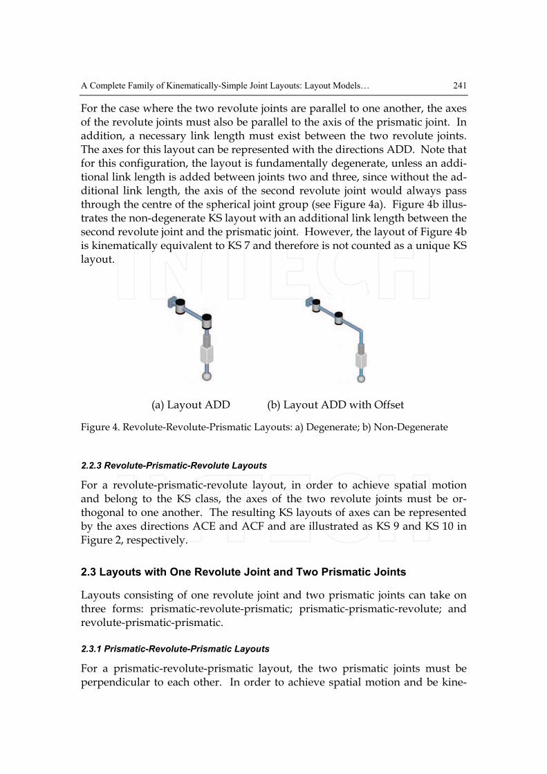
For the case where the two revolute joints are parallel to one another, the axes of the revolute joints must also be parallel to the axis of the prismatic joint. In addition, a necessary link length must exist between the two revolute joints. The axes for this layout can be represented with the directions ADD. Note that for this configuration, the layout is fundamentally degenerate, unless an addi-tional link length is added between joints two and three, since without the ad-ditional link length, the axis of the second revolute joint would always pass through the centre of the spherical joint group (see Figure 4a). Figure 4b illus-trates the non-degenerate KS layout with an additional link length between the second revolute joint and the prismatic joint. However, the layout of Figure 4b is kinematically equivalent to KS 7 and therefore is not counted as a unique KS layout.
(a) Layout ADD
(b) Layout ADD with Offset
Figure 4. Revolute-Revolute-Prismatic Layouts: a) Degenerate; b) Non-Degenerate
2.2.3 Revolute-Prismatic-Revolute Layouts
For a revolute-prismatic-revolute layout, in order to achieve spatial motion and belong to the KS class, the axes of the two revolute joints must be or-thogonal to one another. The resulting KS layouts of axes can be represented by the axes directions ACE and ACF and are illustrated as KS 9 and KS 10 in Figure 2, respectively.
2.3 Layouts with One Revolute Joint and Two Prismatic Joints
Layouts consisting of one revolute joint and two prismatic joints can take on three forms: prismatic-revolute-prismatic; prismatic-prismatic-revolute; and revolute-prismatic-prismatic.
2.3.1 Prismatic-Revolute-Prismatic Layouts
For a prismatic-revolute-prismatic layout, the two prismatic joints must be perpendicular to each other. In order to achieve spatial motion and be kine-

242 Industrial Robotics: Theory, Modelling and Control
matically simple, the axis of the revolute joint must be parallel to the axis of one of the prismatic joints. The feasible layout of joint directions can be repre-sented by the axes directions CFD and is illustrated as KS 11 in Figure 2.
2.3.2 Prismatic-Prismatic-Revolute Layouts
For a prismatic-prismatic-revolute layout, the two prismatic joints must be perpendicular to each other. In order to achieve spatial motion and be kine-matically simple, the axis of the revolute joint must be parallel to one of the prismatic joints. The feasible layout of joint directions can be represented by the axes directions BCF and is illustrated as KS 12 in Figure 2.
2.3.3 Revolute-Prismatic-Prismatic Layouts
For a revolute-prismatic-prismatic layout, the two prismatic joints must be perpendicular to each other. In order to achieve spatial motion and be kine-matically simple, the axis of the revolute joint must be parallel to the axis of one of the prismatic joints. The feasible layout of joint directions can be repre-sented by the axes directions CCD. Note that this layout is kinematically equivalent to the prismatic-revolute-prismatic KS 11. Therefore, the revolute-prismatic-prismatic layout is not kinematically unique. For a further discus-sion on collinear revolute-prismatic axes please see Section 2.5.
2.4 Layouts with Three Prismatic Joints
To achieve spatial motion with three prismatic joints and belong to the KS class, the joint directions must be mutually orthogonal. A representative lay-out of joint directions is CED. This layout is illustrated as KS 13 in Figure 2.
2.5 Additional Kinematically-Simple Layouts
The layouts above represent the 13 layouts with unique kinematics belonging to the KS family. However, additional layouts that have unique joint struc-tures can provide motion that is kinematically equivalent to one of the KS lay-outs. For branches where the axes of a prismatic and revolute joint are collin-ear, there are two possible layouts to achieve the same motion. Four layouts, KS 6, 7, 11, and 12, have a prismatic joint followed by a collinear revolute joint. The order of these joints could be reversed, i.e., the revolute joint could come first followed by the prismatic joint. The order of the joints has no bearing on the kinematics of the layout, but would be very relevant in the physical design of a manipulator. Note that the dj and θj elements of the corresponding rows in the D&H tables (see Section 3.2) would need to be interchanged along with
A Complete Family of Kinematically-Simple Joint Layouts: Layout Models… 243
an appropriate change in subscripts. The presented forward and inverse dis-placement solutions in Sections 4.1 and 4.2 would remain unchanged except for a change in the relevant subscripts. In addition to the above four layouts, as discussed in Section 2.2.2, the layout shown in Figure 4b is kinematically equivalent to KS 7. Therefore, there are five additional kinematically-simple layouts that can be considered part of the KS family.
3. Zero-Displacement Diagrams and D&H Parameters
3.1 Zero-Displacement Diagrams
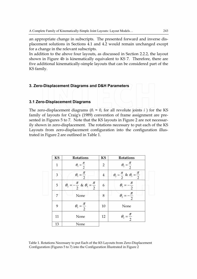
The zero-displacement diagrams (θi = 0, for all revolute joints i ) for the KS family of layouts for Craig's (1989) convention of frame assignment are pre-sented in Figures 5 to 7. Note that the KS layouts in Figure 2 are not necessar-ily shown in zero-displacement. The rotations necessary to put each of the KS Layouts from zero-displacement configuration into the configuration illus-trated in Figure 2 are outlined in Table 1.
KS Rotations KS Rotations
1 2
2
πθ = 2
22
πθ =
3 2
3
πθ = 4
22
πθ = &
23
πθ =
5 2
2
πθ −= &
23
πθ = 6
23
πθ −=
7 None 8 2
2
πθ −=
9 2
3
πθ = 10 None
11 None 12 2
3
πθ =
13 None
Table 1. Rotations Necessary to put Each of the KS Layouts from Zero-Displacement Configuration (Figures 5 to 7) into the Configuration Illustrated in Figure 2
244 Industrial Robotics: Theory, Modelling and Control
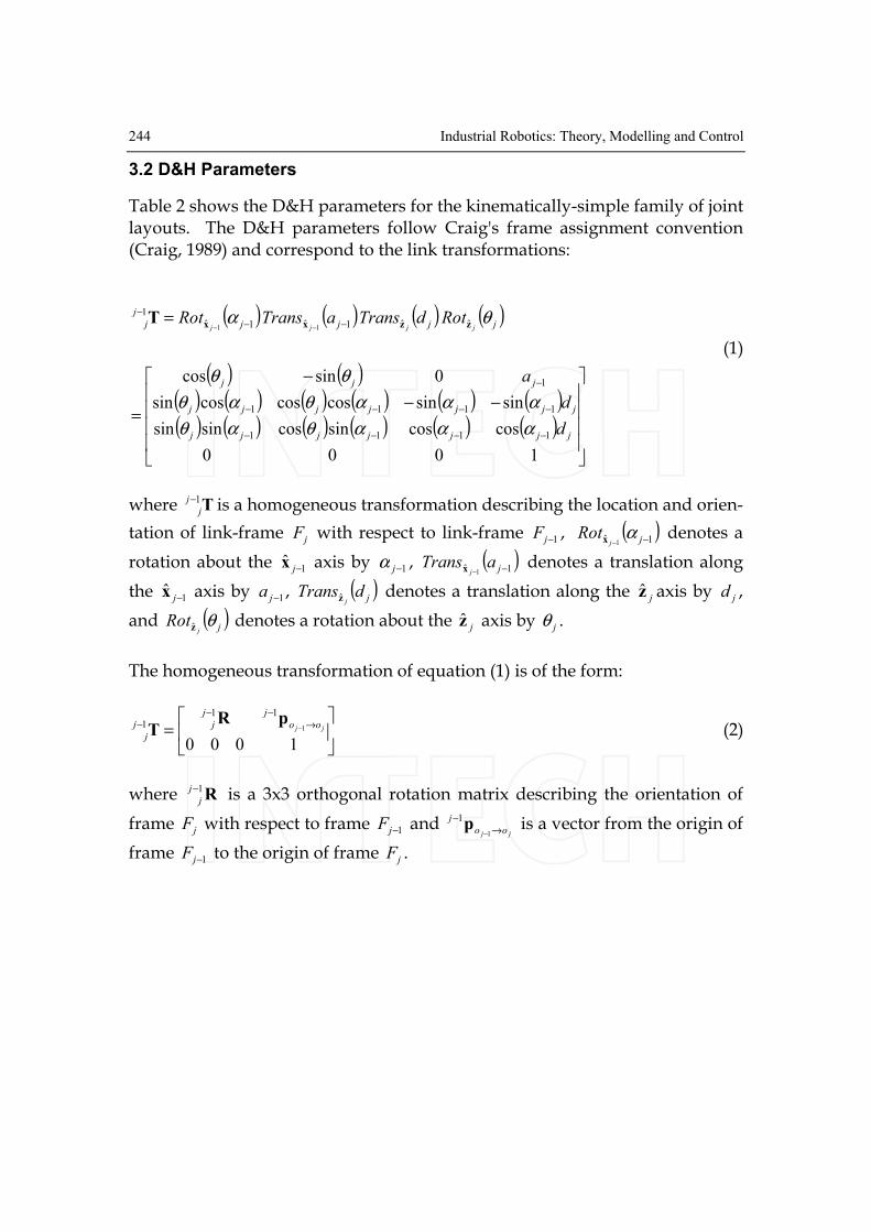
3.2 D&H Parameters
Table 2 shows the D&H parameters for the kinematically-simple family of joint layouts. The D&H parameters follow Craig's frame assignment convention (Craig, 1989) and correspond to the link transformations:
( ) ( ) ( ) ( )
( ) ( )( ) ( ) ( ) ( ) ( ) ( )( ) ( ) ( ) ( ) ( ) ( ) ⎥⎥
⎥⎥
⎦
⎤
⎢⎢⎢⎢
⎣
⎡−−
−
=
=
−−−−
−−−−
−
−−
−
−−
1000
coscossincossinsin
sinsincoscoscossin
0sincos
1111
1111
1
ˆˆ1ˆ1ˆ
1
11
jjjjjjj
jjjjjjj
jjj
jjjj
j
j
d
d
a
RotdTransaTransRotjjjj
αααθαθ
αααθαθ
θθ
θα zzxxT
(1)
where T1−j
j is a homogeneous transformation describing the location and orien-
tation of link-frame jF with respect to link-frame 1−jF , ( )1ˆ 1 −− jjRot αx denotes a
rotation about the 1ˆ
−jx axis by 1−jα , ( )1ˆ 1 −− jaTrans
jx denotes a translation along
the 1ˆ
−jx axis by 1−ja , ( )jdTrans
jz denotes a translation along the jz axis by jd ,
and ( )jj
Rot θz denotes a rotation about the jz axis by jθ .
The homogeneous transformation of equation (1) is of the form:
⎥⎦⎤⎢⎣
⎡= →
−−
− −
10001
11
1 jj oo
jj
jj
j
pRT (2)
where R1−j
j is a 3x3 orthogonal rotation matrix describing the orientation of
frame jF with respect to frame 1−jF and jj oo
j
→
−
−1
1p is a vector from the origin of
frame 1−jF to the origin of frame jF .
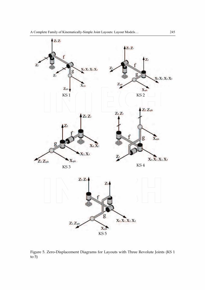
A Complete Family of Kinematically-Simple Joint Layouts: Layout Models… 245
KS 1
KS 2
KS 3
KS 4
KS 5
Figure 5. Zero-Displacement Diagrams for Layouts with Three Revolute Joints (KS 1 to 5)

246 Industrial Robotics: Theory, Modelling and Control
KS 6
KS 7
KS 8
KS 9
KS 10
Figure 6. Zero-Displacement Diagrams for Layouts with Two Revolute Joints and One Prismatic Joint (KS 6 to 10)
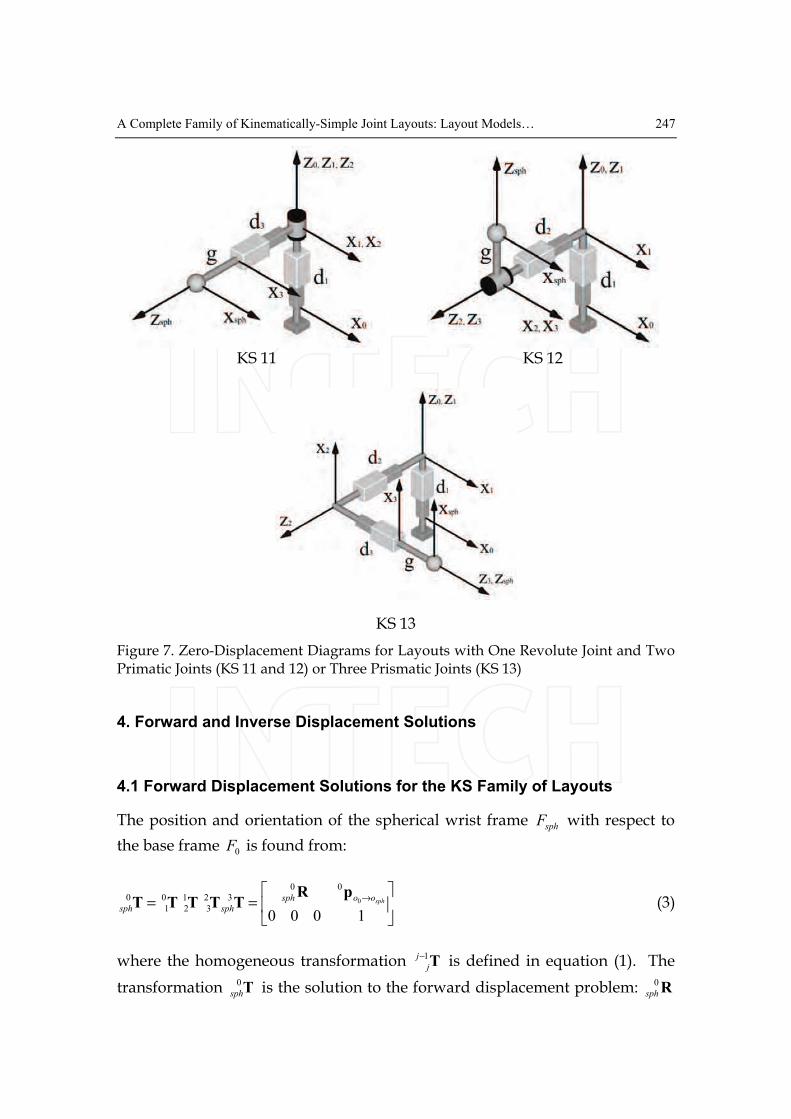
A Complete Family of Kinematically-Simple Joint Layouts: Layout Models… 247
KS 11
KS 12
KS 13
Figure 7. Zero-Displacement Diagrams for Layouts with One Revolute Joint and Two Primatic Joints (KS 11 and 12) or Three Prismatic Joints (KS 13)
4. Forward and Inverse Displacement Solutions
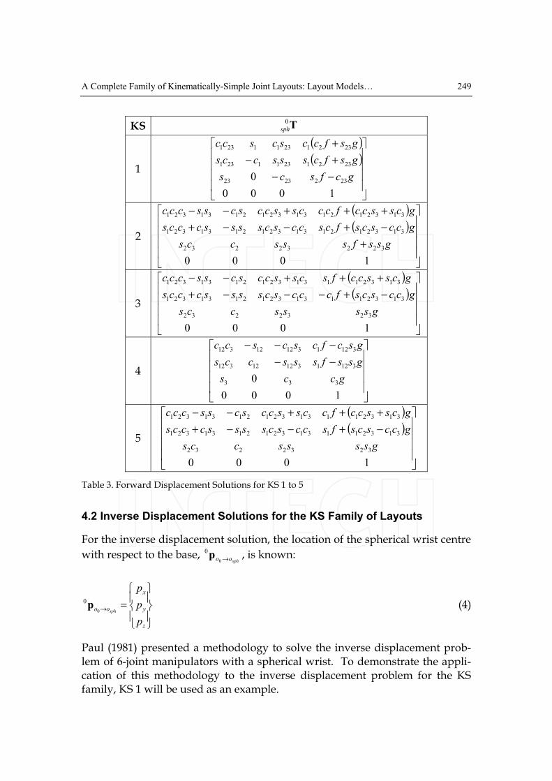
4.1 Forward Displacement Solutions for the KS Family of Layouts
The position and orientation of the spherical wrist frame sphF with respect to
the base frame 0F is found from:
⎥⎦⎤⎢⎣
⎡== →
1000 0
00
32
3
1
2
0
1
0 sphoosph
sphsph
pRTTTTT (3)
where the homogeneous transformation T1−j
j is defined in equation (1). The
transformation T0
sph is the solution to the forward displacement problem: R0
sph
248 Industrial Robotics: Theory, Modelling and Control
is the change in orientation due to the first three joints and sphoo →0
0p is the loca-
tion of the spherical wrist centre. The homogeneous transformations T0
sph for
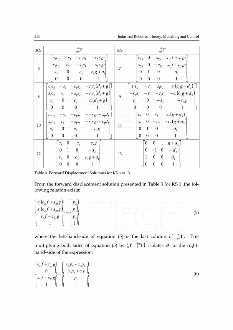
the KS family of layouts can be found in Tables 3 and 4. Note that in Tables 3
and 4, ic and is denote ( )iθcos and ( )iθsin , respectively.
KS 1−jF 1−jα 1−ja jd jθ jF KS 1−jF 1−jα 1−ja jd jθ jF
1 0F 0 0 0 1θ 1F 2
0F 0 0 0 1θ 1F
1F 2/π 0 0 2θ 2F
1F 2/π 0 0 2θ 2F
2F 0 f 0 3θ 3F
2F 2/π− f 0 3θ 3F
3F 2/π 0 g 0 sphF 3F 2/π 0 g 0 sphF
3 0F 0 0 0 1θ 1F 4
0F 0 0 0 1θ 1F
1F 2/π 0 f 2θ 2F
1F 0 f 0 2θ 2F
2F 2/π− 0 0 3θ 3F
2F 2/π 0 0 3θ 3F
3F 2/π 0 g 0 sphF 3F 2/π− 0 g 0 sphF
5 0F 0 0 0 1θ 1F 6
0F 0 0 1d 0
1F
1F 2/π f 0 2θ 2F
1F 0 0 0 2θ 2F
2F 2/π− 0 0 3θ 3F
2F 2/π 0 0 3θ 3F
3F 2/π 0 g 0 sphF 3F 2/π− 0 g 0 sphF
7 0F 0 0 1d 0
1F 8 0F 0 0 0
1θ 1F
1F 0 0 0 2θ 2F
1F 2/π 0 0 2θ 2F
2F 0 f 0 3θ 3F
2F 2/π− 0 3d 0
3F
3F 2/π 0 g 0 sphF 3F 0 0 g 0 sphF
9 0F 0 0 0 1θ 1F 10
0F 0 0 0 1θ 1F
1F 2/π 0 2d 2/π 2F
1F 2/π 0 2d 0
2F
2F 2/π 0 0 3θ 3F
2F 0 0 0 3θ 3F
3F 2/π− 0 g 0 sphF 3F 2/π− 0 g 0 sphF
11 0F 0 0 1d 0
1F 12 0F 0 0
1d 0 1F
1F 0 0 0 2θ 2F
1F 2/π 0 2d 0
2F
2F 2/π 0 3d 0
3F 2F 0 0 0
3θ 3F
3F 0 0 g 0 sphF 3F 2/π− 0 g 0 sphF
13 0F 0 0 1d 0
1F
1F 2/π 0 2d 2/π 2F
2F 2/π 0 3d 0
3F
3F 0 0 g 0 sphF
Table 2. D&H Parameters for the KS Layouts
A Complete Family of Kinematically-Simple Joint Layouts: Layout Models… 249
KS T0
sph
1
( )
( )
⎥⎥⎥⎥
⎦
⎤
⎢⎢⎢⎢
⎣
⎡−−
+−
+
1000
0 2322323
23212311231
23212311231
gcfscs
gsfcsssccs
gsfccscscc
2
( )
( )
⎥⎥⎥⎥
⎦
⎤
⎢⎢⎢⎢
⎣
⎡+
−+−−+
+++−−
1000
32232232
3132121313212131321
3132121313212131321
gssfsssccs
gccscsfcsccscsssscccs
gcssccfcccssccscssccc
3
( )
( )
⎥⎥⎥⎥
⎦
⎤
⎢⎢⎢⎢
⎣
⎡−+−−−+
+++−−
1000
3232232
313211313212131321
313211313212131321
gssssccs
gccscsfcccscsssscccs
gcssccfscssccscssccc
4
⎥⎥⎥⎥
⎦
⎤
⎢⎢⎢⎢
⎣
⎡−−
−−−
1000
0 333
312131212312
312131212312
gccs
gssfsssccs
gscfcscscc
5
( )
( )
⎥⎥⎥⎥
⎦
⎤
⎢⎢⎢⎢
⎣
⎡−+−−+
+++−−
1000
3232232
313211313212131321
313211313212131321
gssssccs
gccscsfsccscsssscccs
gcssccfccssccscssccc
Table 3. Forward Displacement Solutions for KS 1 to 5
4.2 Inverse Displacement Solutions for the KS Family of Layouts
For the inverse displacement solution, the location of the spherical wrist centre
with respect to the base, sphoo →0
0p , is known:
⎪⎭⎪⎬⎫
⎪⎩⎪⎨⎧
=→
z
y
x
oo
p
p
p
sph0
0p (4)
Paul (1981) presented a methodology to solve the inverse displacement prob-lem of 6-joint manipulators with a spherical wrist. To demonstrate the appli-cation of this methodology to the inverse displacement problem for the KS family, KS 1 will be used as an example.
250 Industrial Robotics: Theory, Modelling and Control
KS T0
sph KS T0
sph
6
⎥⎥⎥⎥
⎦
⎤
⎢⎢⎢⎢
⎣
⎡+
−−
−−−
1000
0 1333
3232232
3232232
dgccs
gssssccs
gscscscc
7
⎥⎥⎥⎥
⎦
⎤
⎢⎢⎢⎢
⎣
⎡−−
+
1000
010
0
0
1
2322323
2322323
d
gcfscs
gsfcsc
8
( )
( )
( ) ⎥⎥⎥⎥
⎦
⎤
⎢⎢⎢⎢
⎣
⎡+
+−−
+−−−
1000
0 3222
32121121
32121121
gdccs
gdssssccs
gdscscscc
9
( )
( )
⎥⎥⎥⎥
⎦
⎤
⎢⎢⎢⎢
⎣
⎡−−
+−−−−
+−
1000
0 333
23131131
23131131
gssc
dgccccssc
dgcscscss
10
⎥⎥⎥⎥
⎦
⎤
⎢⎢⎢⎢
⎣
⎡−−−
+−−−
1000
0 333
213131131
213131131
gccs
dcgssssccs
dsgscscscc
11
( )
( )
⎥⎥⎥⎥
⎦
⎤
⎢⎢⎢⎢
⎣
⎡+−−
+
1000
010
0
0
1
3222
3222
d
dgccs
dgssc
12
⎥⎥⎥⎥
⎦
⎤
⎢⎢⎢⎢
⎣
⎡+
−
−−
1000
0
010
0
1333
2
333
dgccs
d
gssc
13
⎥⎥⎥⎥
⎦
⎤
⎢⎢⎢⎢
⎣
⎡−−
+
1000
001
010
100
1
2
3
d
d
dg
Table 4. Forward Displacement Solutions for KS 6 to 13
From the forward displacement solution presented in Table 3 for KS 1, the fol-lowing relation exists:
( )
( )
⎪⎪⎭⎪⎪⎬⎫
⎪⎪⎩⎪⎪⎨⎧
=
⎪⎪⎭⎪⎪⎬⎫
⎪⎪⎩⎪⎪⎨⎧
−
+
+
11
232
2321
2321
z
y
x
p
p
p
gcfs
gsfcs
gsfcc
(5)
where the left-hand-side of equation (5) is the last column of T0
sph . Pre-
multiplying both sides of equation (5) by ( ) 10
1
1
0
−
= TT isolates 1θ to the right-
hand-side of the expression:
⎪⎪⎭⎪⎪⎬⎫
⎪⎪⎩⎪⎪⎨⎧
+−
+
=
⎪⎪⎭⎪⎪⎬⎫
⎪⎪⎩⎪⎪⎨⎧
−
+
11
0 11
11
232
232
z
yx
yx
p
pcps
pspc
gcfs
gsfc
(6)
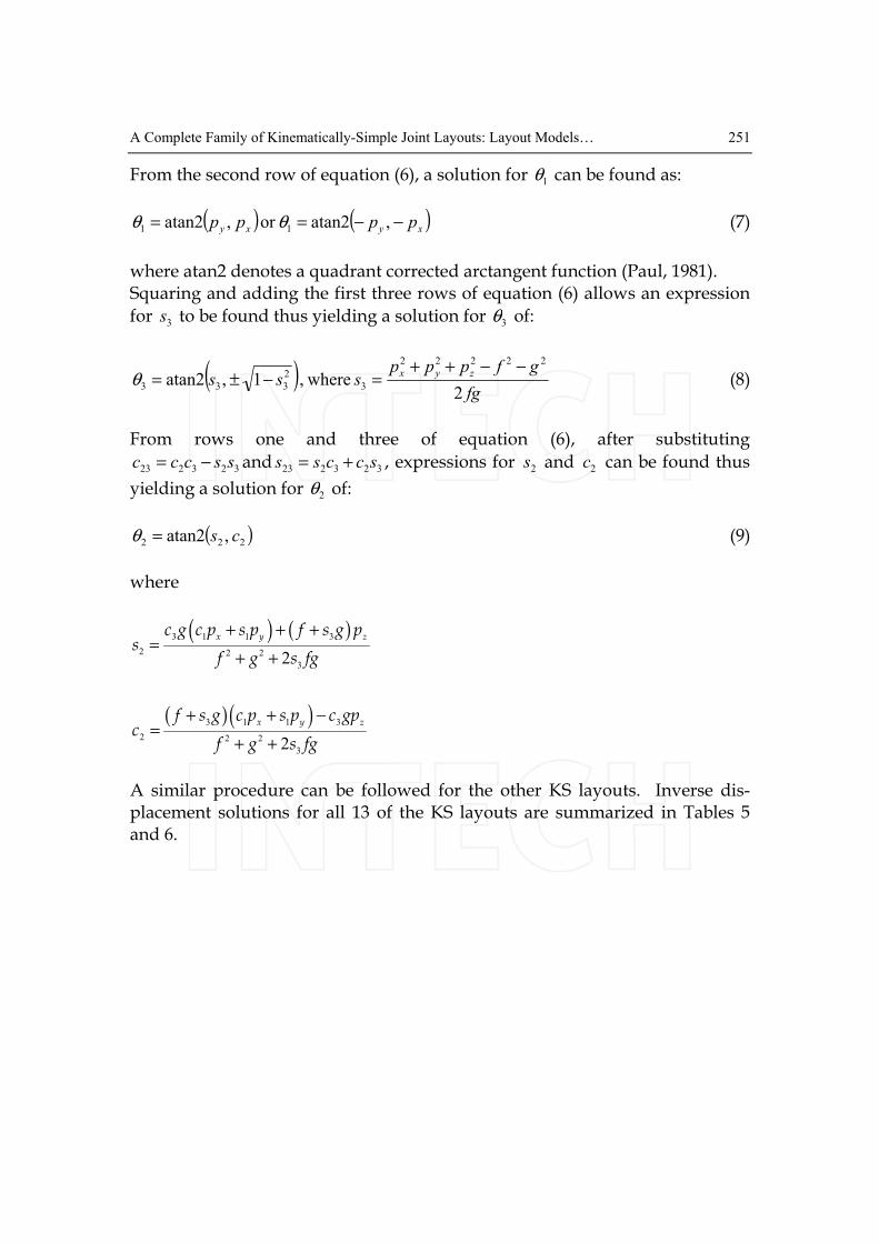
A Complete Family of Kinematically-Simple Joint Layouts: Layout Models… 251
From the second row of equation (6), a solution for 1θ can be found as:
( ) ( ) ,atan2or ,atan2 11 xyxy pppp −−== θθ (7)
where atan2 denotes a quadrant corrected arctangent function (Paul, 1981). Squaring and adding the first three rows of equation (6) allows an expression
for 3s to be found thus yielding a solution for 3θ of:
( ) 2
where, 1 ,atan2
22222
3
2
333fg
gfpppsss
zyx −−++=−±=θ (8)
From rows one and three of equation (6), after substituting
323223 ssccc −= and 323223 sccss += , expressions for 2s and 2c can be found thus
yielding a solution for 2θ of:
( )222 ,atan2 cs=θ (9)
where
( ) ( )
( )( )
3 1 1 3
2 2 2
3
3 1 1 3
2 2 2
3
2
2
x y z
x y z
c g c p s p f s g ps
f g s fg
f s g c p s p c gpc
f g s fg
+ + +=
+ +
+ + −=
+ +
A similar procedure can be followed for the other KS layouts. Inverse dis-placement solutions for all 13 of the KS layouts are summarized in Tables 5 and 6.
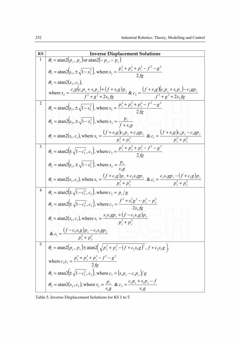
252 Industrial Robotics: Theory, Modelling and Control
KS Inverse Displacement Solutions 1 ( ) ( ) ,atan2or ,atan21 xyxy pppp −−=θ
( ) 2
where, 1 ,atan2
22222
3
2
333fg
gfpppsss
zyx −−++=−±=θ
( ) , ,atan2 222 cs=θ
( ) ( ) ( )( )
2 &
2 where
3
22
3113
2
3
22
3113
2fgsgf
gpcpspcgsfc
fgsgf
pgsfpspcgcs
zyxzyx
++
−++=
++
+++=
2 ( )
2 where, 1 ,atan2
22222
3
2
333fg
gfpppsss
zyx −−++=−±=θ
( ) where, 1 ,atan23
2
2
222gsf
psss z
+=−±=θ
( )( ) ( )
22
323
122
323
1111 & where, ,atan2yx
yx
yx
xy
pp
gpcpcgsfc
pp
gpcpcgsfscs
+
−+=
+
++==θ
3 ( )
2 where, ,1atan2
22222
33
2
33fg
gfpppccc
zyx −−++=−±=θ
( ) where, 1 ,atan23
2
2
222gs
psss z=−±=θ
( )( ) ( )
22
332
122
323
1111 & where, ,atan2yx
yx
yx
yx
pp
pgcfgpscc
pp
gpscpgcfscs
+
+−=
+
++==θ
4 ( ) where, ,1atan2 33
2
33 gpccc z=−±=θ
( ) 2
where, ,1atan23
2222
3
2
22
2
22fgs
ppgsfccc
yx −−+=−±=θ
( )( )
( )22
3232
1
22
3232
1111
&
where, ,atan2
yx
yx
yx
yx
pp
gpsspgscfc
pp
pgscfgpssscs
+
−−=
+
−+==θ
5 ( ) ( ) , ,atan2 ,atan2 32
2
32
22
1 ⎟⎠⎞⎜⎝⎛ ++−+±= gscfgscfpppp yxxyθ
2
where
22222
32fg
gfpppsc
zyx −−++=
( ) ( ) where, ,1atan2 1133
2
33 gpcpsccc yx −=−±=θ
( )gs
fpspcc
gs
pscs
yxz
3
11
2
3
2222 & where, ,atan2−+
===θ
Table 5. Inverse Displacement Solutions for KS 1 to 5

A Complete Family of Kinematically-Simple Joint Layouts: Layout Models… 253
KS Inverse Displacement Solutions
6 222
1 gpppd yxz +−−±=
( ) ( ) where, ,1atan2 133
2
33 gdpccc z −=−±=θ
( )gs
pc
gs
pscs xy
3
2
3
2222 & where, ,atan2−
=−
==θ
7 zpd =1
( ) 2
where, 1 ,atan2
2222
3
2
333fg
gfppsss
yx −−+=−±=θ
( )( )
( )
( )
( ) & where, ,atan2
22
3
2
3
33
222
3
2
3
33
2222gcgsf
gpcpgsfc
gcgsf
pgsfgpcscs
yxyx
++
−+=
++
++==θ
8 ( ) ( ) ,atan2or ,atan21 xyxy pppp −−=θ
gpppd zyx −++±=222
3
( )gd
pc
gd
pspcscs zyx
+=
+
−−==
3
2
3
11
2222 & where, ,atan2θ
9 ( ) ( ) ,atan2or ,atan21 yxyx pppp −−=θ
22
112 zyx pgpcpsd −±−=
( ) ( ) gdpcpscgpscs yxz 21133333 & where, ,atan2 −−=−==θ
10 ( ) gpccc z=−±= 33
2
33 where, ,1atan2θ
22
3
22
2 gsppd yx −+±=
( )22
23
122
23
1111 & where, ,atan2yx
yx
yx
xy
pp
pdgpsc
pp
pdgpsscs
+
−−=
+
+−==θ
11 zpd =1
gppd yx −+±=22
3
( )gd
pc
gd
pscs
yx
+
−=
+==
3
2
3
2222 & where, ,atan2θ
12 ypd −=2
22
1 gppd xz +−±=
( ) ( ) gdpcgpscs zx 133333 & where, ,atan2 −=−==θ
13 gpd x −=3
ypd −=2
zpd =1
Table 6. Inverse Displacement Solutions for KS 6 to 13
254 Industrial Robotics: Theory, Modelling and Control
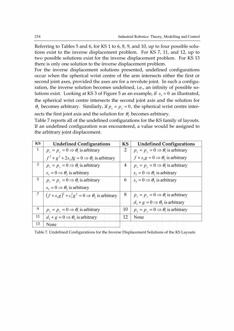
Referring to Tables 5 and 6, for KS 1 to 6, 8, 9, and 10, up to four possible solu-tions exist to the inverse displacement problem. For KS 7, 11, and 12, up to two possible solutions exist for the inverse displacement problem. For KS 13 there is only one solution to the inverse displacement problem. For the inverse displacement solutions presented, undefined configurations occur when the spherical wrist centre of the arm intersects either the first or second joint axes, provided the axes are for a revolute joint. In such a configu-ration, the inverse solution becomes undefined, i.e., an infinity of possible so-
lutions exist. Looking at KS 3 of Figure 5 as an example, if 03 =s as illustrated,
the spherical wrist centre intersects the second joint axis and the solution for
2θ becomes arbitrary. Similarly, if 0== yx pp , the spherical wrist centre inter-
sects the first joint axis and the solution for 1θ becomes arbitrary.
Table 7 reports all of the undefined configurations for the KS family of layouts. If an undefined configuration was encountered, a value would be assigned to the arbitrary joint displacement. KS Undefined Configurations KS Undefined Configurations 1 arbitrary is 0 1θ⇒== yx pp
arbitrary is 02 23
22 θ⇒=++ fgsgf
2 arbitrary is 0 1θ⇒== yx pp
arbitrary is 0 23 θ⇒=+ gsf
3 arbitrary is 0 1θ⇒== yx pp
arbitrary is 0 23 θ⇒=s
4 arbitrary is 0 1θ⇒== yx pp
arbitrary is 0 23 θ⇒=s
5 arbitrary is 0 1θ⇒== yx pp
arbitrary is 0 23 θ⇒=s
6 arbitrary is 0 23 θ⇒=s
7 ( ) arbitrary is 0 2
22
3
2
3 θ⇒=++ gcgsf 8 arbitrary is 0 1θ⇒== yx pp
arbitrary is 0 23 θ⇒=+ gd
9 arbitrary is 0 1θ⇒== yx pp 10 arbitrary is 0 1θ⇒== yx pp
11 arbitrary is 0 23 θ⇒=+ gd 12 None
13 None
Table 7. Undefined Configurations for the Inverse Displacement Solutions of the KS Layouts

A Complete Family of Kinematically-Simple Joint Layouts: Layout Models… 255
5. Discussion
5.1 Application of the KS Layouts
The KS family of layouts can be used as main-arms for serial manipulators or as branches of parallel manipulators. For example, KS 1 is a common main-arm layout for numerous industrial serial manipulators. KS 4 is the branch configuration used in the RSI Research 6-DOF Master Controller parallel joy-stick (Podhorodeski, 1991). KS 8 is a very common layout used in many paral-lel manipulators including the Stewart-Gough platform (Stewart, 1965-66). KS 13 is the layout used in Cartesian manipulators. The choice of which KS layout to use for a manipulator would depend on fac-tors such as the shape of the desired workspace, the ease of manufacture of the manipulator, the task required, etc. For example, layout KS 1 provides a large spherical workspace. Having the second and third joints parallel in KS 1 al-lows for the motors of the main-arm to be mounted close to the base and a simple drive-train can used to move the third joint.
5.2 Reconfigurable Manipulators
KS layouts are also very useful for reconfigurable manipulators. Podhorode-ski and Nokleby (2000) presented a Reconfigurable Main-Arm (RMA) manipu-lator capable of configuring into all five KS layouts comprised of revolute only joints (KS 1 to 5). Depending on the task required, one of the five possible lay-outs can be selected. Yang, et al. (2001) showed how KS branches are useful for modular recon-figurable parallel manipulators.
5.3 Application of the Presented Displacement Solutions
5.3.1 Serial Manipulators
If a KS layout is to be used as a main-arm of a serial manipulator, the spherical wrist needs to be actuated. Figure 8 shows the zero-displacement configura-tion and Table 8 the D&H parameters for the common roll-pitch-roll spherical-wrist layout. The wrist shown in Figure 8 can be attached to any of the KS layouts.

256 Industrial Robotics: Theory, Modelling and Control
Figure 8. Zero-Displacement Diagram for the Roll-Pitch-Roll Spherical Wrist
1−jF 1−jα 1−ja jd jθ jF
sphF 0 0 0 4θ 4F
4F 2/π− 0 0 5θ 5F
5F 2/π 0 0 6θ 6F
Table 8. D&H Parameters for the Roll-Pitch-Roll Spherical Wrist
For the KS family of layouts with a spherical wrist, the forward displacement solution is:
( )( ) TTTTTTTTTTTT6
6
065
6
4
54
32
3
1
2
0
1
0 ee
sph
sphee
sph
sphee == (10)
where T6
ee is the homogeneous transformation describing the end-effector
frame eeF with respect to frame 6F and would be dependent on the type of
tool attached, T0
sph is defined in equation (3), and Tsph
6 is:
⎥⎥⎥⎥
⎦
⎤
⎢⎢⎢⎢
⎣
⎡−
+−+
−−−
=
1000
0
0
0
56565
546465464654
546465464654
6csscs
ssccscsscccs
sccssccssccc
sphT (11)
For a 6-joint serial manipulator, Pieper (1968) demonstrated that for a manipu-lator with three axes intersecting, a closed-form solution to the inverse dis-placement problem can be found. As demonstrated by Paul (1981), for a 6-joint manipulator with a spherical wrist, the solutions for the main-arm and wrist displacements can be solved separately. Therefore, the presented inverse

A Complete Family of Kinematically-Simple Joint Layouts: Layout Models… 257
displacement solutions for the KS family of layouts (see Section 4.2) can be used to solve for the main-arm joint displacements for serial manipulators that use KS layouts as their main-arm and have a spherical wrist. For the inverse displacement solution of the main-arm joints, the location
(60
0
oo →p ) and orientation ( R0
6 ) of frame 6F with respect to the base frame in
terms of the known value T0
ee can be found from:
( ) ⎥⎦⎤⎢⎣
⎡=== →
1000 60
00
6
6
01-600
6
ooee
eeeeee
pRTTTTT (12)
where Tee6 is constant and known. Since the manipulator has a spherical wrist:
⎪⎭⎪⎬⎫
⎪⎩⎪⎨⎧
==== →→→→
z
y
x
oooooooo
p
p
p
sph 4050600
0000 pppp (13)
where xp , yp , and zp are found from equation (12). The inverse displacement
solutions for the KS family of layouts discussed in Section 4.2 can now be used to solve for the main-arm joint displacements. For the inverse displacement solution of the spherical wrist joints, in terms of
the known value T0
ee , the orientation of 6F with respect to the base frame, R0
6 ,
was defined in equation (12). Note that:
⎥⎥⎥⎦
⎤⎢⎢⎢⎣
⎡===
333231
232221
131211
0
6
3
0
0
6
0
3
3
6
rrr
rrr
rrrT
RRRRR (14)
Since the main arm joint displacements were solved above, the elements of
matrix R3
0 are known values and thus the right-hand-side of equation (14) is
known, i.e., ijr , i = 1 to 3 and j = 1 to 3, are known values.
Substituting the elements of the rotation matrix RRRsph
sph 6
33
6 = into equation
(14) yields:
⎥⎥⎥⎦
⎤⎢⎢⎢⎣
⎡=
⎥⎥⎥⎦
⎤⎢⎢⎢⎣
⎡−
+−+
−−−
==
333231
232221
131211
56565
546465464654
546465464654
3
6
33
6
rrr
rrr
rrr
csscs
ssccscsscccs
sccssccssccc
sph
sph
sph RRRR (15)
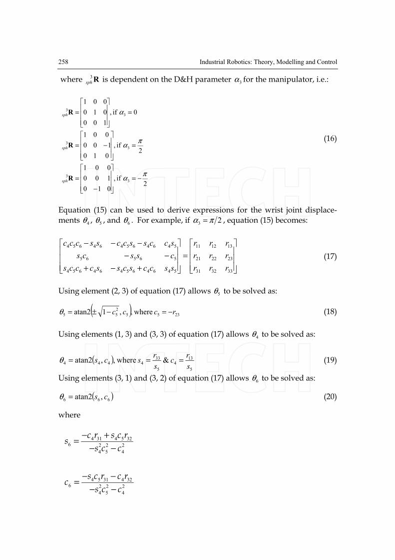
258 Industrial Robotics: Theory, Modelling and Control
where R3
sph is dependent on the D&H parameter 3α for the manipulator, i.e.:
2 if ,
010
100
001
2 if ,
010
100
001
0 if ,
100
010
001
3
3
3
3
3
3
πα
πα
α
−=
⎥⎥⎥⎦
⎤⎢⎢⎢⎣
⎡−
=
=
⎥⎥⎥⎦
⎤⎢⎢⎢⎣
⎡−=
=
⎥⎥⎥⎦
⎤⎢⎢⎢⎣
⎡=
R
R
R
sph
sph
sph
(16)
Equation (15) can be used to derive expressions for the wrist joint displace-
ments 4θ , 5θ , and 6θ . For example, if 23 πα = , equation (15) becomes:
⎥⎥⎥⎦
⎤⎢⎢⎢⎣
⎡=
⎥⎥⎥⎦
⎤⎢⎢⎢⎣
⎡+−+
−−
−−−
333231
232221
131211
546465464654
56565
546465464654
rrr
rrr
rrr
ssccscsscccs
csscs
sccssccssccc
(17)
Using element (2, 3) of equation (17) allows 5θ to be solved as:
( ) 2355
2
55 where, ,1atan2 rccc −=−±=θ (18)
Using elements (1, 3) and (3, 3) of equation (17) allows 4θ to be solved as:
( ) & where, ,atan25
134
5
334444
s
rc
s
rscs ===θ (19)
Using elements (3, 1) and (3, 2) of equation (17) allows 6θ to be solved as:
( )666 ,atan2 cs=θ (20)
where
4 31 4 5 32
6 2 2 2
4 5 4
4 5 31 4 32
6 2 2 2
4 5 4
c r s c rs
s c c
s c r c rc
s c c
− +=
− −
− −=
− −

A Complete Family of Kinematically-Simple Joint Layouts: Layout Models… 259
Note that if 05 =s , joint axes 4 and 6 are collinear and the solutions for 4θ and
6θ are not unique. In this case, 4θ can be chosen arbitrarily and 6θ can be
solved for.
Similar solutions can be found for the cases where 3α equals 0 and 2π− .
5.3.2 Parallel Manipulators
Two frames common to the branches of the parallel manipulator are estab-
lished, one frame attached to the base ( baseF ) and the other attached to the plat-
form ( platF ). The homogeneous transformations from the base frame baseF to
the base frame of each of the m branches i
F0 are denoted Tbase
i0 , i = 1 to m. The
homogeneous transformations from the platform frame platF to the m passive
spherical group frames isphF are denoted T
plat
sphi, i = 1 to m. Note that for a given
parallel manipulator all Tbase
i0 and Tplat
sphi would be known and would be con-
stant. For the inverse displacement solution, for the ith branch, the location and orien-
tation of the spherical wrist frame, isphF , with respect to the base frame of the
branch, i
F0 , in terms of the known value Tbase
plat can be found from:
( ) ⎥⎦⎤⎢⎣
⎡=== →
1000 0
0001-
0
0isphi
ii
i
i
i
ii
i
i
oosphplat
sph
base
platbase
plat
sph
base
plat
base
sph
pRTTTTTTT (21)
where Riisph
0 is the orientation of isphF with respect to
iF0 and
isphi
i
oo →0
0p is the po-
sition vector from the origin of i
F0 to the origin of isphF with respect to
iF0 . The
position vector is defined as:
⎪⎭⎪⎬⎫
⎪⎩⎪⎨⎧
=→
i
i
i
isphi
i
z
y
x
oo
p
p
p
0
0p (22)
where ix
p , iy
p , and izp are known values. The inverse displacement solutions
for the KS family of layouts shown in Section 4.2 can then be used to solve for the joint displacements for branches i =1 to m. Unlike the forward displacement problem of serial manipulators, the forward displacement problem of parallel manipulators is challenging. Raghavan
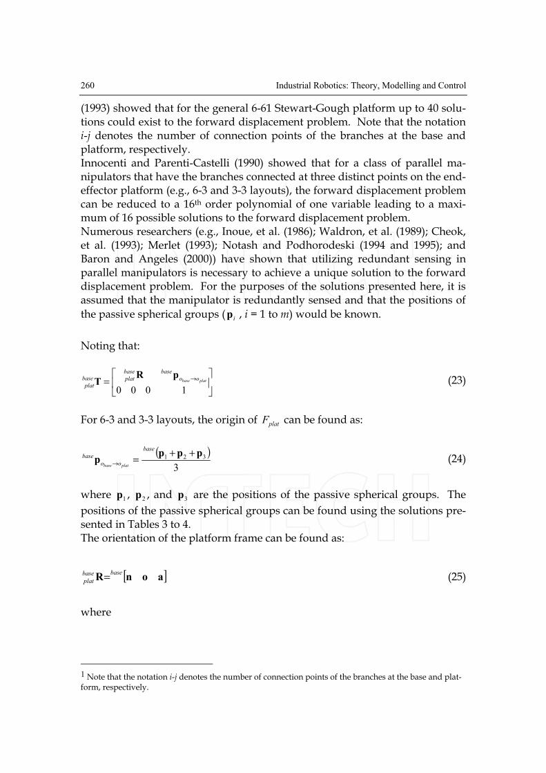
260 Industrial Robotics: Theory, Modelling and Control
(1993) showed that for the general 6-61 Stewart-Gough platform up to 40 solu-tions could exist to the forward displacement problem. Note that the notation i-j denotes the number of connection points of the branches at the base and platform, respectively. Innocenti and Parenti-Castelli (1990) showed that for a class of parallel ma-nipulators that have the branches connected at three distinct points on the end-effector platform (e.g., 6-3 and 3-3 layouts), the forward displacement problem can be reduced to a 16th order polynomial of one variable leading to a maxi-mum of 16 possible solutions to the forward displacement problem. Numerous researchers (e.g., Inoue, et al. (1986); Waldron, et al. (1989); Cheok, et al. (1993); Merlet (1993); Notash and Podhorodeski (1994 and 1995); and Baron and Angeles (2000)) have shown that utilizing redundant sensing in parallel manipulators is necessary to achieve a unique solution to the forward displacement problem. For the purposes of the solutions presented here, it is assumed that the manipulator is redundantly sensed and that the positions of
the passive spherical groups ( ip , i = 1 to m) would be known.
Noting that:
⎥⎦⎤⎢⎣
⎡= →
1000platbase oo
basebase
platbase
plat
pRT (23)
For 6-3 and 3-3 layouts, the origin of platF can be found as:
( )3
321 pppp
++=→
base
oo
base
platbase (24)
where 1p , 2p , and 3p are the positions of the passive spherical groups. The
positions of the passive spherical groups can be found using the solutions pre-sented in Tables 3 to 4. The orientation of the platform frame can be found as:
[ ]aonRbasebase
plat = (25)
where
1 Note that the notation i-j denotes the number of connection points of the branches at the base and plat-form, respectively.

A Complete Family of Kinematically-Simple Joint Layouts: Layout Models… 261
nao
cn
cna
pp
ppn
basebasebase
basebase
basebasebase
base
base
23
23
×=
×
×=
⎟⎟⎠⎞
⎜⎜⎝⎛
−
−=
with
⎟⎟⎠⎞
⎜⎜⎝⎛
−
−=
21
21
pp
ppc
base
base
For 6-6 and 3-6 layouts, the origin of platF can be found as:
( )6
654321 ppppppp
+++++=→
base
oo
base
platbase
(26)
where 1p to 6p are the positions of the passive spherical groups. Note that it is
assumed that the passive spherical groups are symmetrically distributed about the platform. The positions of the passive spherical groups can be found using the solutions presented in Tables 3 and 4. The orientation of the platform frame can be found as:
[ ]aonRbasebase
plat = (27)
where
nao
cn
cna
pp
ppn
basebasebase
basebase
basebasebase
bc
bc
base
base
×=
×
×=
⎟⎟⎠⎞
⎜⎜⎝⎛
−
−=
with
( )
( )
( ) 2
2
2
65
43
21
ppp
ppp
ppp
pp
ppc
+=
+=
+=
−
−=
c
b
a
ba
babase
262 Industrial Robotics: Theory, Modelling and Control
6. Conclusions
The complete set of layouts belonging to a kinematically simple (KS) family of spatial joint layouts were presented. The considered KS layouts were defined as ones in which the manipulator (or branch of a parallel manipulator) incor-porates a spherical group of joints at the wrist with a main-arm comprised of successfully parallel or perpendicular joints with no unnecessary offsets or lengths between joints. It was shown that there are 13 layouts having unique kinematics belonging to the KS family: five layouts comprised of three revolute joints; five layouts comprised of two revolute joints and one prismatic joint; two layouts comprised of one revolute joint and two prismatic joints; and one layout comprised of three prismatic joints. In addition, it was shown that there are a further five kinematically-simple lay-outs having unique joint structures, but kinematics identical to one of the 13 KS layouts. Zero-displacement diagrams, D&H parameters, and the complete forward and inverse displacement solutions for the KS family of layouts were presented. It was shown that for the inverse displacement problem up to four possible solu-tions exist for KS 1 to 6, 8, 9, and 10, up to two possible solutions exist for KS 7, 11, and 12, and only one solution exists for KS 13. The application of the KS family of joint layouts and the application of the presented forward and in-verse displacement solutions to both serial and parallel manipulators was dis-cussed.
Acknowledgements
The authors wish to thank the Natural Sciences and Engineering Research Council (NSERC) of Canada for providing funding for this research.

A Complete Family of Kinematically-Simple Joint Layouts: Layout Models… 263
7. References
Baron, L. & Angeles, J. (2000). The Direct Kinematics of Parallel Manipulators Under Joint-Sensor Redundancy. IEEE Transactions on Robotics and Automation, Vol. 16, No. 1, pp. 12-19.
Cheok, K. C.; Overholt, J. L. & Beck, R. R. (1993). Exact Methods for Determin-ing the Kinematics of a Stewart Platform Using Additional Displace-ment Sensors. Journal of Robotic Systems, Vol. 10, No. 5, pp. 689-707.
Craig, J. J. (1989). Introduction To Robotics: Mechanics and Control - Second Edi-tion, Addison-Wesley Publishing Company, Don Mills, Ontario, Can-ada.
Denavit, J. & Hartenberg, R. S. (1955). A Kinematic Notation for Lower-Pair Mechanisms Based on Matrices. Transactions of the ASME, Journal of Ap-plied Mechanics, June, pp. 215-221.
Innocenti, C. & Parenti-Castelli, V. (1990). Direct Position Analysis of the Stewart Platform Mechanism. Mechanism and Machine Theory, Vol. 25, No. 6, pp. 611-621.
Inoue, H.; Tsusaka, Y. & and Fukuizumi, T. (1986). Parallel Manipulator, In: Robotics Research: The Third International Symposium, Faugeras, O. D. & Giralt, G., (Ed.), pp. 321-327, MIT Press, Cambridge, Massachusetts, USA.
Merlet, J.-P. (1993). Closed-Form Resolution of the Direct Kinematics of Paral-lel Manipulators Using Extra Sensors Data, Proceedings of the 1993 IEEE International Conference on Robotics and Automation - Volume 1, May 2-6, 1993, Atlanta, Georgia, USA, pp. 200-204.
Notash, L. & Podhorodeski, R. P. (1994). Complete Forward Displacement So-lutions for a Class of Three-Branch Parallel Manipulators. Journal of Ro-botic Systems, Vol. 11, No. 6, pp. 471-485.
Notash, L. & Podhorodeski, R. P. (1995). On the Forward Displacement Prob-lem of Three-Branch Parallel Manipulators. Mechanism and Machine Theory, Vol. 30, No. 3, pp. 391-404.
Paul, R. P. (1981). Robot Manipulators: Mathematics, Programming, and Control, MIT Press, Cambridge, Massachusetts, USA.
Pieper, D. L. (1968). The Kinematics of Manipulators Under Computer Control. Ph.D. Dissertation, Stanford University, Stanford, California, USA.
Podhorodeski, R. P. (1991). A Screw Theory Based Forward Displacement So-lution for Hybrid Manipulators, Proceedings of the 2nd National Applied Mechanisms and Robotics Conference - Volume I, November 3-6, 1991, Cin-cinnati, Ohio, USA, pp. IIIC.2--1 - IIIC.2-7.
Podhorodeski, R. P. (1992). Three Branch Hybrid-Chain Manipulators: Struc-ture, Displacement, Uncertainty and Redundancy Related Concerns, Proceedings of the 3rd Workshop on Advances in Robot Kinematics, Septem-ber 7-9, 1992, Ferrara, Italy, pp. 150-156.

264 Industrial Robotics: Theory, Modelling and Control
Podhorodeski, R. P. & Nokleby, S. B. (2000). Reconfigurable Main-Arm for As-sembly of All Revolute-Only Kinematically Simple Branches. Journal of Robotic Systems, Vol. 17, No. 7, pp. 365-373.
Podhorodeski, R. P. & Pittens, K. H. (1992). A Class of Hybrid-Chain Manipu-lators Based on Kinematically Simple Branches, Proceedings of the 1992 ASME Design Technical Conferences - 22nd Biennial Mechanisms Conference, September 13-16, 1992, Phoenix, Arizona, USA, pp. 59-64.
Podhorodeski, R. P. & Pittens, K. H. (1994). A Class of Parallel Manipulators Based on Kinematically Simple Branches. Transactions of the ASME, Journal of Mechanical Design, Vol. 116, No. 3, pp. 908-914.
Raghavan, M. (1993). The Stewart Platform of General Geometry Has 40 Con-figurations. Transactions of the ASME, Journal of Mechanical Design, Vol. 115, No. 2, pp. 277-282.
Stewart, D. (1965-66). A Platform With Six Degrees of Freedom. Proceedings of the Institution of Mechanical Engineers, Vol. 180, Part 1, No. 15, pp. 371-386.
Waldron, K. J.; Raghavan, M. & Roth, B. (1989). Kinematics of a Hybrid Series-Parallel Manipulation System. Transactions of the ASME, Journal of Dy-namic Systems, Measurement, and Control, Vol. 111, No. 2, pp. 211-221.
Yang, G.; Chen, I.-M.; Lim, W. K. & Yeo, S. H. (2001). Kinematic Design of Modular Reconfigurable In-Parallel Robots. Autonomous Robots, Vol. 10,
Issue 1, pp. 83-89.
Industrial Robotics: Theory, Modelling and ControlEdited by Sam Cubero
ISBN 3-86611-285-8Hard cover, 964 pagesPublisher Pro Literatur Verlag, Germany / ARS, Austria Published online 01, December, 2006Published in print edition December, 2006
InTech EuropeUniversity Campus STeP Ri Slavka Krautzeka 83/A 51000 Rijeka, Croatia Phone: +385 (51) 770 447 Fax: +385 (51) 686 166www.intechopen.com
InTech ChinaUnit 405, Office Block, Hotel Equatorial Shanghai No.65, Yan An Road (West), Shanghai, 200040, China
Phone: +86-21-62489820 Fax: +86-21-62489821
This book covers a wide range of topics relating to advanced industrial robotics, sensors and automationtechnologies. Although being highly technical and complex in nature, the papers presented in this bookrepresent some of the latest cutting edge technologies and advancements in industrial robotics technology.This book covers topics such as networking, properties of manipulators, forward and inverse robot armkinematics, motion path-planning, machine vision and many other practical topics too numerous to list here.The authors and editor of this book wish to inspire people, especially young ones, to get involved with roboticand mechatronic engineering technology and to develop new and exciting practical applications, perhaps usingthe ideas and concepts presented herein.
How to referenceIn order to correctly reference this scholarly work, feel free to copy and paste the following:
Scott Nokleby and Ron Podhorodeski (2006). A Complete Family of Kinematically-Simple Joint Layouts: LayoutModels, Associated Displacement Problem Solutions and Applications, Industrial Robotics: Theory, Modellingand Control, Sam Cubero (Ed.), ISBN: 3-86611-285-8, InTech, Available from:http://www.intechopen.com/books/industrial_robotics_theory_modelling_and_control/a_complete_family_of_kinematically-simple_joint_layouts__layout_models__associated_displacement_prob


![CIT 384: Network AdministrationSlide #1 CIT 384: Network Administration Routing ][](https://img.pdfslide.net/doc/110x75/56649f4a5503460f94c6bec3/cit-384-network-administrationslide-1-cit-384-network-administration-routing.jpg)