1

A Brief on Climate Downscaling: Motivation, Approaches,

Applications, Discussions

David Yates and David GochisNational Center for Atmospheric Research

31 May 2011

2

Outline

• Climate downscaling Motivation• Overview of RAL’s Climate Four Dimensional

Data Assimilation System• Overview of the NCAR Nested Regional Climate

Model• Examples of downscaled climate information

3

Science Questions:

Questions:• How will precipitation change over key river basin?

– Seasonality– Phase– Intensity

• What is the influence of the precipitation changes on terrestrial hydrology?– SWE (peak, seasonal accumulation and ablation)– Soil moisture and ET– Runoff

4

Climate downscaling methods

• Empirical or statistical techniques− Identify links between large-scale climate elements

(predictors) and local climate (the predictand), and apply to output from global or regional models. Terrain elevation and slope. Land cover (forest, water body, crop land). Historical meteorological measurements. Expert knowledge.

• Dynamical techniques – Explicitly predicts the physical processes of the

climate system.

5

Downscaling Paradigms:

• Emphasizes range of probabilities over process

• More complete in terms of distribution of outcomes

• Applies suspect assumptions in ‘cross-scale’ interpretations

• Can’t account for many ‘non-linearites’ in climate system processes

• Neglects, rigorous process evaluation

6

Downscaling Paradigms:

• Emphasizes process over representation

• Identifies processes behind the ‘answer’

• Accounts for changes in dynamical and microphysical structures (e.g. non-linear impacts)

• Neglects the plausible range of likely outcomes

7

Downscaling Paradigms:

• Emphasizes range of probabilities over process

• More complete in terms of distribution of outcomes

• Applies suspect assumptions in ‘cross-scale’ interpretations

• Can’t account for many ‘non-linearites’ in climate system processes

• Neglects, rigorous process evaluation

• Emphasizes process over representation

• Identifies processes behind the ‘answer’

• Accounts for changes in dynamical and microphysical structures (e.g. non-linear impacts)

• Neglects the plausible range of likely outcomes

88

Statistical downscaling

• A statistical regression between local climate variables and large scale predictors (e.g., large scale atmospheric flow local temperature).

• Example: Model output statistics (MOS).

`

Predictors (Global/Regional Model)

Predictands (values at local scale)

large-scale analysis

local value

9

Dynamical Downscaling

• Empirical or statistical techniques− Identify links between large-scale climate elements

(predictors) and local climate (the predictand), and apply to output from global or regional models. Terrain elevation and slope. Land cover (forest, water body, crop land). Historical meteorological measurements. Expert knowledge.

• Dynamical techniques – Explicitly predicts the physical processes of the

climate system.

10Source: Clifford Mass, Univ. Washington

Global scale data mapped to local regionwhile adding small scale variability

Process-Based Climate Downscaling

11

Dynamical downscaling

• Limited area model (LAM) “embedded” within a global model.– Global model

constrains LAM.

– LAM defines small scale features.

– Information only passed from global model to LAM.

LAMgrid

Global analysis

12

Statistical versus dynamical downscaling

Source: Clifford Mass, Univ. of Washington

Statistical downscaling• Cheap.• Makes simplifying

assumptions about how local weather works.

• Statistical relationships might not be valid if climate undergoes change.

Dynamical downscaling• Computationally

Expensive.• Physical systems explicitly

predicted.• May produce local trends

not depicted by global models.

13

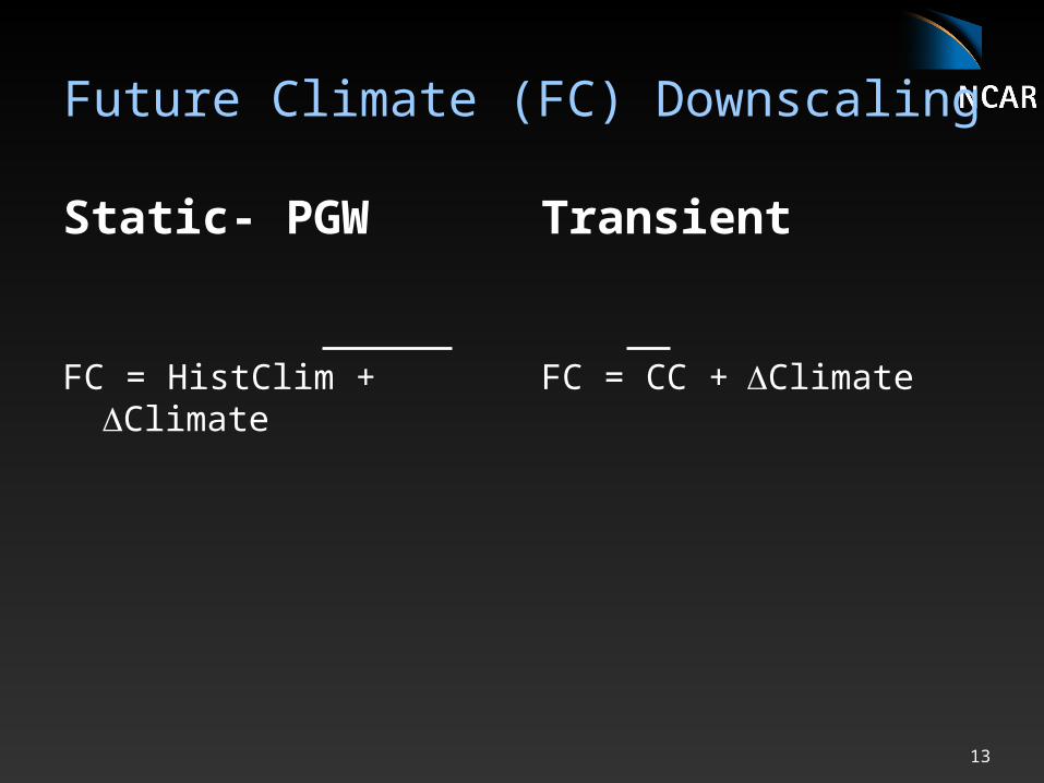
Future Climate (FC) Downscaling

Static- PGW

FC = HistClim + Climate

Transient

FC = CC +Climate

14

Static “Pseudo-Global Warming” (SPGW)

1. Derive Difference field : U, V, T, geopot. hgt., Psfc and Qv between current and future climate periods from a CGCM

2. Add difference to current period atmospheric conditions (North American Regional Reanalysis, 3-hrly) (2.0 oC temperature increase over Colorado, and an increase of mixing ratio on the order of 15 - 20%.)

Caveat: No change in transient spectra (i.e. same climate variability in the future

except for changes in storms within the domain)

Monthly mean of past condition

CCSM 1995-2005

Monthly mean of past condition

CCSM 1995-2005

Monthly mean of future condition

CCSM 2045-2055

Monthly mean of future condition

CCSM 2045-2055

15

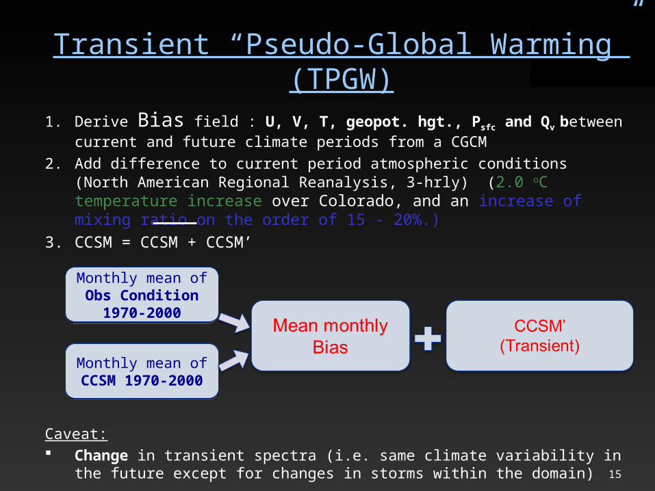
Transient “Pseudo-Global Warming” (TPGW)

1. Derive Bias field : U, V, T, geopot. hgt., Psfc and Qv between current and future climate periods from a CGCM

2. Add difference to current period atmospheric conditions (North American Regional Reanalysis, 3-hrly) (2.0 oC temperature increase over Colorado, and an increase of mixing ratio on the order of 15 - 20%.)

3. CCSM = CCSM + CCSM’

Caveat: Change in transient spectra (i.e. same climate variability in the future

except for changes in storms within the domain)

Monthly mean of Obs Condition

1970-2000

Monthly mean of Obs Condition

1970-2000

Monthly mean of CCSM 1970-2000Monthly mean of CCSM 1970-2000

16

17

Imposed Warming Experiment:

Current

Future-Current

Future

500mb Wind and Geopotential Height500mb Wind and Geopotential Height

All positive changes

18

Imposed Warming Experiment:

Current

Future-Current

Future

19

Imposed Warming Experiment:

Current

Future-Current

Future

500mb RH500mb RH

Current

Future-Current

Future

20

Assessing Climate Phase: Mean Annual Cycle

Precipitation Temperature

21

Motivation

• Large-scale climate models use horizontal grid increments of 60-300 km.

• Consequence or impact models require grid increments of 10 km or smaller.

Source: David Viner, Climatic Res. Unit, Univ. of East Anglia, UK.

22

Motivation

• Seasonal, yearly, inter-annual to decadal climate variability strongly impacts society.

−Water resources.− Flood risk.− Spread of infectious disease.− Energy demand and production.− Building design and construction.−Regional transport and dispersion.− Locating weather-sensitive installations (airports).− Locating new observing systems.

23

Science Questions:Questions:• How will precipitation change over river basin?

– Seasonality– Phase– Intensity

• What is the influence of precipitation changes on terrestrial hydrology?– Snow Water (peak, seasonal accumulation and ablation)– Soil moisture and ET– Runoff

Pprocess/physics-based approach:• Interested in identifying the processes

behind the ‘answer’• Ability to consistently account for

changes in dynamical and microphysical structures (e.g. non-linear impacts)

24

How will vulnerability to dengue evolve with climate and land use changes?

NRCM: Impacts of climate change on spread of disease

25

CCSM3 (~150 km resolution)

NRCM(20 km resolution)

1800 UTC 2-m temperature difference for March 2057-2059 and March 2007-2009.

Map

(Simulations performed by Cody Phillips, NSAP)

NRCM: Impacts of climate change on spread of disease

26

CCSMNRCMNRCM DOMAINS

Temperature (deg C)

GDF SUEZ interested in impacts of climate change on a proposed wind farm near the Belgian coast.

Comparison of CCSM and NRCM wind vectors, near-surface temperature (colors), and sea level pressure (blue lines) for 1200 UTC 02 January 2020.

D_01

D_02

D_03

NRCM: Impacts of climate change on wind energy production