3D Models of Vibration Isolation Systems in Mathematica

April 12th,2011

Takanori Sekiguchi

Concept

Three-dimensional rigid-body models in Mathematica

Inspired by Mark Barton’s suspension models

http://www.ligo.caltech.edu/~e2e/SUSmodels/

The model can provide eigenfrequencies and eigenmodes of the system (with 3D

Graphics), transfer functions from disp to disp, and from force/torque to disp of every

6 DOFs of the given objects.

Asymmetry in geometry, wire length, stiffness, and etc. may be taken into account.

The simulation provides state-space matrices of the system and exports them to a

MATLAB code, for studying active controls and etc.

Method of Calculation

(1) Express the potential energy EP, kinetic energy EK and damping energy ED of the

system in terms of the coordinates and coordinate velocities.

),,(),,,,,,(),,,( 1111 nDDnnKKnPP xxEExxxxEExxEE

(2) Minimize the potential energy EP to find the equilibrium points of the system.

),,( )()(1)( eqneqeq xxx

(3) Differentiate the potential energy of the system with respect to pairs of coordinates

at equilibrium to create the stiffness matrix K. In a similar way, differentiate the

kinetic energy and damping energy with respect to coordinate velocities to create the

mass matrix M and damping matrix G.

)()()(

,,

eqeqeq xxji

Dij

xxji

Kij

xxji

Pij

xx

EG

xx

EM

xx

EK

(4) Do diagonalization of the stiffness and mass matrices to obtain the eigenfrequencies

and eigenmodes of the system.

iii eeKM 21 )(

(5) Calculate transfer functions of the system from the stiffness, mass and damping

matrices.

More details are in LIGO-T020205-02-D (“Models of the Advanced LIGO Suspensions in

Mathematica” by Mark Barton).

Potential Terms

Wires

Assume a wire as a massless beam, with a spring constant defined by its young’s

modulus, length and diameter. The potential energy of each wire is broken up in two

terms, longitudinal stretching energy and torsional energy.

torsiontorsionstretchl

GJElxlE

0

2

02

1,))((

2

1

Springs (GAS Filters)

A spring is taken to join two points in different objects and apply restoring forces and

pre-load forces to them. The potential energy is given by:

Roll

Yaw

Pitch

z

y

x

f

Roll

Yaw

Pitch

z

y

x

KRollYawPitchzyxE preloadspringspring ),,,,,(2

1.

Coordinate System

(VIRGO's Reference)

X-axis: Transversal, Y-axis: Vertical, Z-axis: Longitudinal (Beam-axis)

Pitch: Rotation around x-axis, Yaw: Rotation around y-axis, Roll: Rotation around z-axis

Demonstration

1. Simple Pendulum (Suspending LIGO mirror with four 50-cm wires)

Parameters Body (Test Mass)

mTM=10.7kg;(*Mass*)

ixTM=0.051kg meter2;(*MOI around x-axis*)

iyTM=0.051kg meter2;(*MOI around y-axis*)

izTM=0.078kg meter2;(*MOI around z-axis*)

iTM={{ixTM,0,0},{0,iyTM,0},{0,0,izTM}};(*MOI Tensor*)

rTM=12.5cm;(*radius*)

lTM=10cm;(*length*)

shapeTM="Cylinder";(*Body Shape*)

Geometry

dzTM=3cm;(*z-separation of wires *)

dxTM=25cm;(*x-separation of wires *)

dyTM=1mm;(*height of wire break-off above COM at TM*)

Wires

lNwire={50,50,50,50}cm;(*Natural length*)

dwire={0.20,0.20,0.20,0.20}mm;(*Diameter*)

matwire={"W","W","W","W"};(*Material*)

The attachment points for wires (in local body coordinate)

clampu={{-dxu/2,0,+dzu/2},{+dxu/2,0,+dzu/2},{-dxu/2,0,-dzu/2},{+dxu/2,0,-dzu/2}};

clampl={{-dxl/2,dyTM,+dzl/2},{+dxl/2,dyTM,+dzl/2},{-dxl/2,dyTM,-dzl/2},{+dxl/2,dyTM,-dzl/2}};

Initial Position & Orientation

lw=50cm;(*typical wire length*)

initg={0,0,0,0,0,0};(*Ground*)

initTM={0,-lw,0,0,0,0};(*Test Mass*)

Equilibrium Point of the System {xTM0.,yTM-0.502016,zTM0.,pitchTM0.,yawTM0.,rollTM0.}

Eigen Mode List {N, Freq, Type(Amplitude)},

{1, 0.70425, zTM(-0.999956)},

{2, 0.704253, xTM(-1.)},

{3, 1.28425, yawTM(1.)},

{4, 3.40524, pitchTM(-1.)},

{5, 15.6376, yTM(1.)},

{6, 22.8949, rollTM(-1.)}

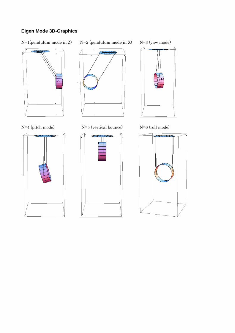
Eigen Mode 3D-Graphics

N=1(pendulum mode in Z) N=2 (pendulum mode in X) N=3 (yaw mode)

N=4 (pitch mode) N=5 (vertical bounce) N=6 (roll mode)

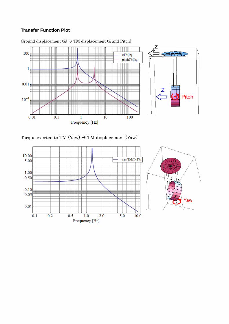
Transfer Function Plot

Ground displacement (Z) TM displacement (Z and Pitch)

Torque exerted to TM (Yaw) TM displacement (Yaw)

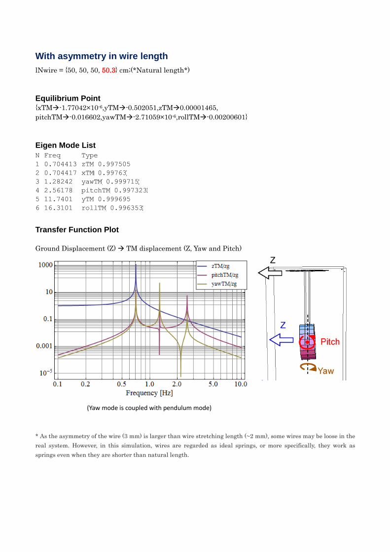
With asymmetry in wire length

lNwire = {50, 50, 50, 50.3} cm;(*Natural length*)

Equilibrium Point {xTM-1.77042×10-6,yTM-0.502051,zTM0.00001465,

pitchTM-0.016602,yawTM-2.71059×10-6,rollTM-0.00200601}

Eigen Mode List

Transfer Function Plot

Ground Displacement (Z) TM displacement (Z, Yaw and Pitch)

(Yaw mode is coupled with pendulum mode)

* As the asymmetry of the wire (3 mm) is larger than wire stretching length (~2 mm), some wires may be loose in the

real system. However, in this simulation, wires are regarded as ideal springs, or more specifically, they work as

springs even when they are shorter than natural length.

N Freq Type

1 0.704413 zTM 0.997505

2 0.704417 xTM 0.99763

3 1.28242 yawTM 0.999715

4 2.56178 pitchTM 0.997323

5 11.7401 yTM 0.999695

6 16.3101 rollTM 0.996353

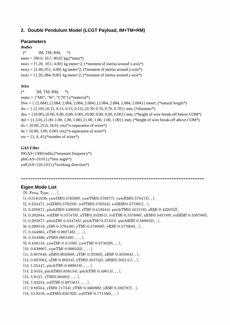
2. Double Pendulum Model (LCGT Payload, IM+TM+RM)

Parameters Bodies

(* IM, TM, RM, *)

mass = {80.0, 10.7, 90.0} kg;(*mass*)

moix = {1.20, .051, 4.00} kg meter^2; (*moment of inertia around x-axis*)

moiy = {2.40,.051, 4.00} kg meter^2; (*moment of inertia around y-axis*)

moiz = {1.20,.084, 8.00} kg meter^2; (*moment of inertia around z-axis*)

Wire

(* IM, TM, RM, *)

matw = {"MS", "W", "C70"};(*material*)

lNw = { {2.084},{2.084, 2.084, 2.084, 2.084},{2.084, 2.084, 2.084, 2.084}} meter; (*natural length*)

dw = { {2.10},{0.15, 0.15, 0.15, 0.15},{0.70, 0.70, 0.70, 0.70}} mm; (*diameter*)

dyu = {{0.00},{0.00, 0.00, 0.00, 0.00},{0.00, 0.00, 0.00, 0.00}} mm; (*height of wire break-off below COM*)

dyl = {{-3.0},{1.00, 1.00, 1.00, 1.00},{1.00, 1.00, 1.00, 1.00}} mm; (*height of wire break-off above COM*)

dx = {0.00, 25.0, 34.0} cm;(*x-separation of wires*)

dz = {0.00, 3.00, 6.00} cm;(*z-separation of wires*)

nw = {1, 4, 4};(*number of wires*)

GAS Filter

f0GAS={300}mHz;(*resonant frequency*)

phiGAS={0.01};(*loss angle*)

wdGAS={{0,1,0}};(*working direction*)

Eigen Mode List {N, Freq, Type, , , , },

{1, 0.0161036, yawIM(0.576599), yawTM(0.576977), yawRM(0.578473), , },

{2, 0.223471, rollIM(0.576258), rollTM(0.576524), rollRM(0.577891), , },

{3, 0.259871, pitchIM(0.439005), zTM(-0.418244), pitchTM(0.451518), zRM(-0.422052)},

{4, 0.262844, rollIM(-0.337478), xTM(0.552851), rollTM(-0.337686), xRM(0.545749), rollRM(-0.338786)},

{5, 0.293877, pitchIM(-0.554785), pitchTM(-0.57433), pitchRM(-0.599832), , },

{6, 0.299516, yIM(-0.576436), yTM(-0.578006), yRM(-0.577608), , },

{7, 0.344863, xTM(-0.992746), , , , },

{8, 0.344886, zTM(0.990168), , , , },

{9, 0.456134, yawIM(-0.41356), yawTM(-0.873029), , , },

{10, 0.639907, yawTM(-0.999322), , , , },

{11, 0.687048, zIM(0.902068), zTM(-0.30365), zRM(-0.305064), , },

{12, 0.687064, xIM(-0.90234), xTM(0.303722), xRM(0.305141), , },

{13, 1.25447, pitchTM(-0.999818), , , , },

{14, 2.0554, pitchIM(0.838134), pitchTM(-0.49613), , , },

{15, 5.8127, yTM(0.99493), , , , },

{16, 7.83234, rollTM(-0.997561), , , , },

{17, 9.88554, yIM(0.71734), yTM(-0.366096), yRM(-0.592787), , },

{18, 10.9316, rollIM(0.630762), rollTM(-0.771166), , , }

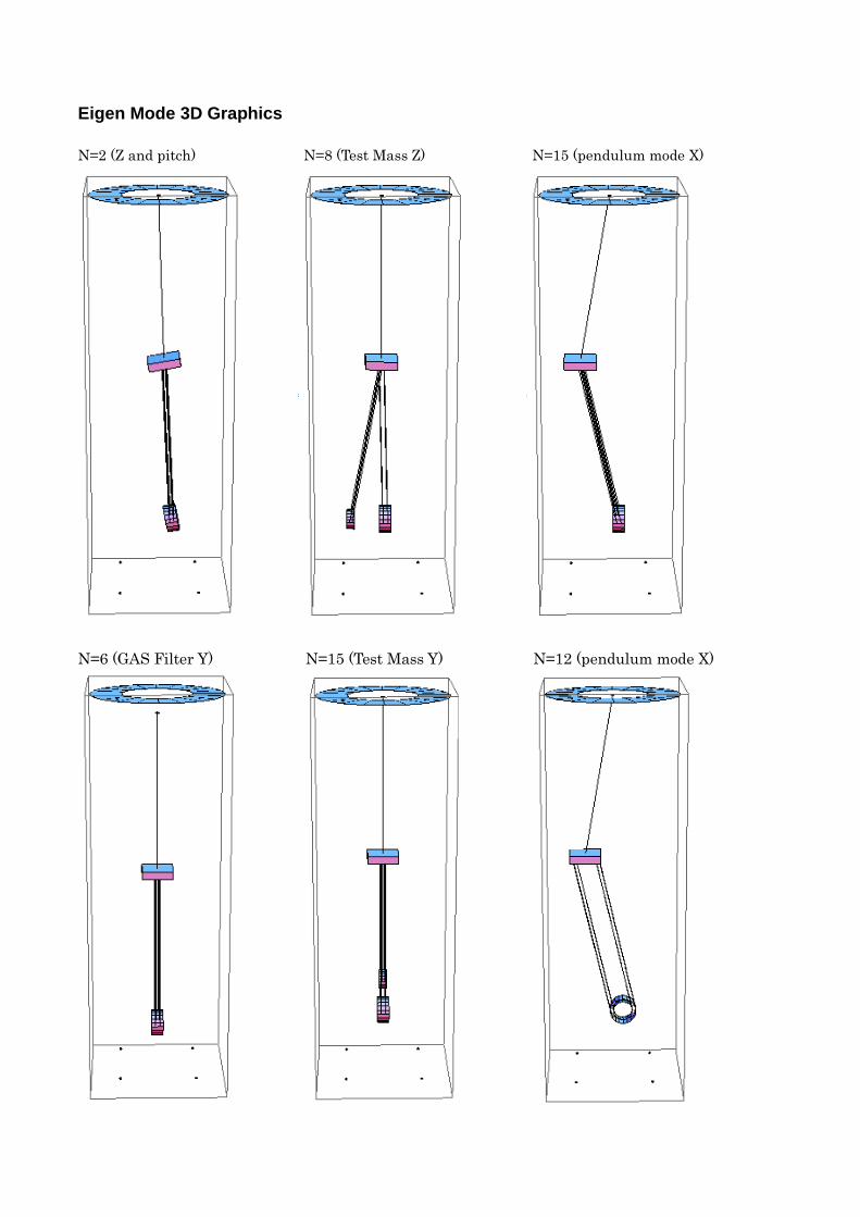
Eigen Mode 3D Graphics

N=2 (Z and pitch) N=8 (Test Mass Z) N=15 (pendulum mode X)

N=6 (GAS Filter Y) N=15 (Test Mass Y) N=12 (pendulum mode X)

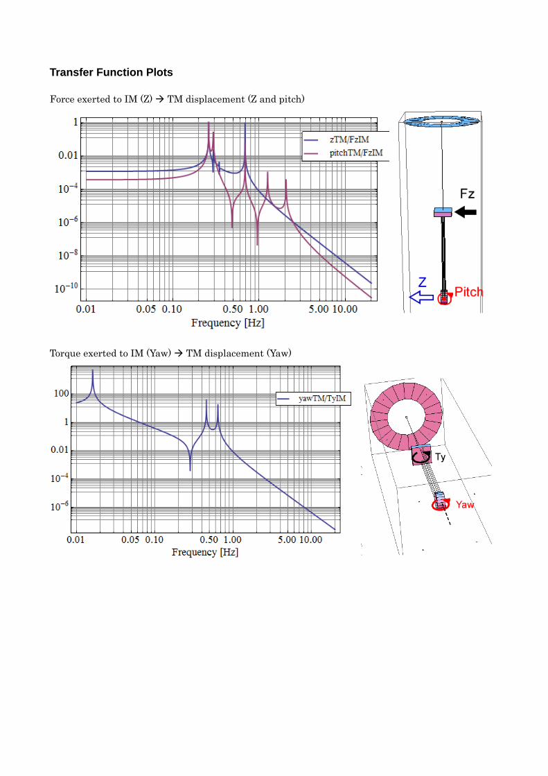
Transfer Function Plots

Force exerted to IM (Z) TM displacement (Z and pitch)

Torque exerted to IM (Yaw) TM displacement (Yaw)

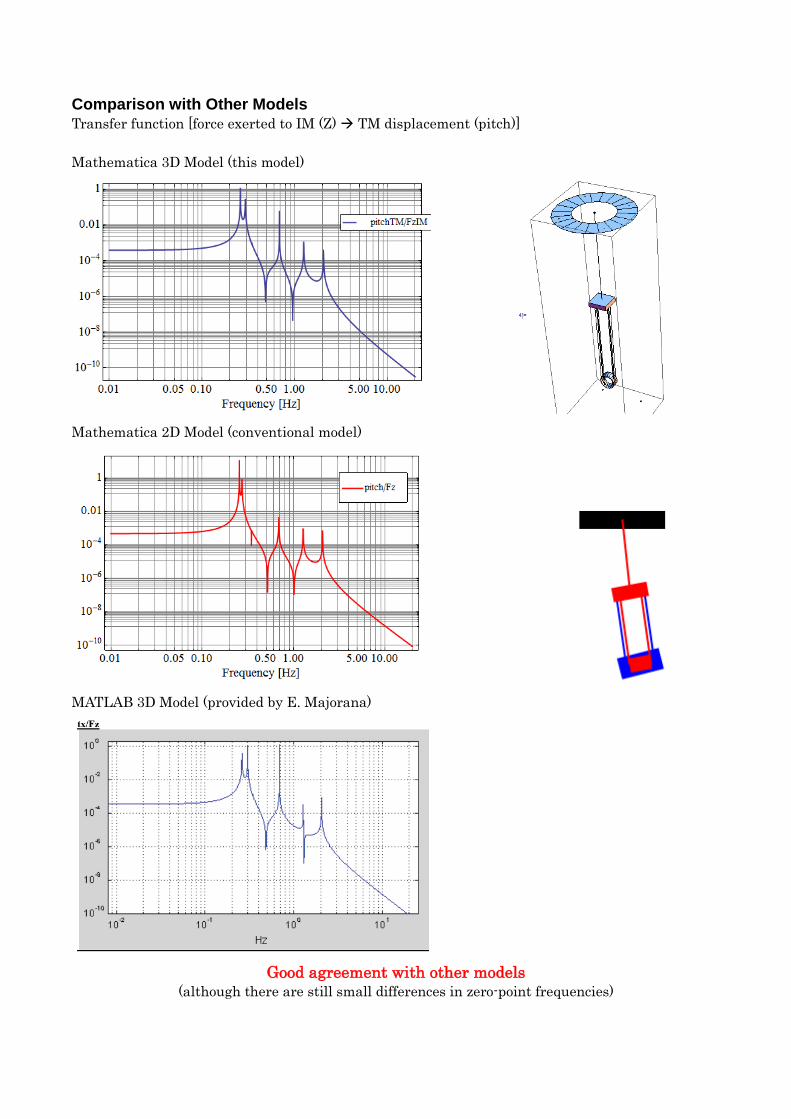
Comparison with Other Models

Transfer function [force exerted to IM (Z) TM displacement (pitch)]

Mathematica 3D Model (this model)

Mathematica 2D Model (conventional model)

MATLAB 3D Model (provided by E. Majorana)

Good agreement with other models (although there are still small differences in zero-point frequencies)

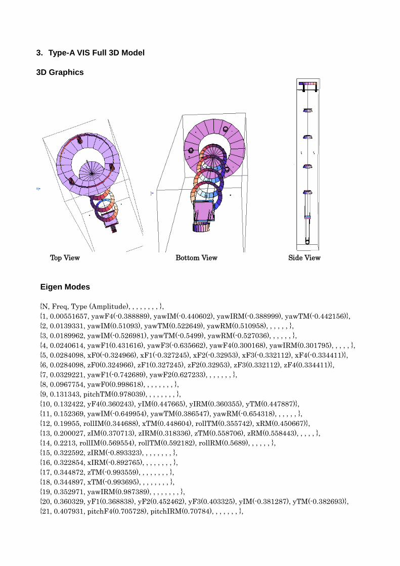
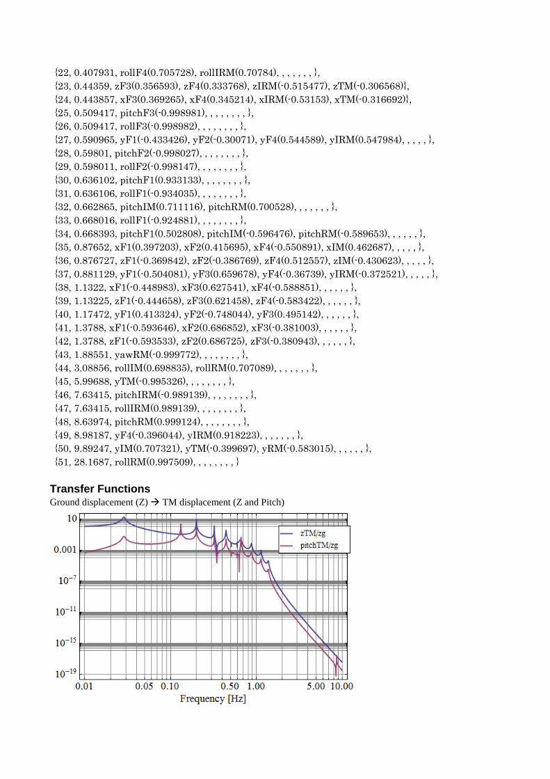
3. Type-A VIS Full 3D Model

3D Graphics

Top View Bottom View Side View

Eigen Modes

{N, Freq, Type (Amplitude), , , , , , , , },

{1, 0.00551657, yawF4(-0.388889), yawIM(-0.440602), yawIRM(-0.388999), yawTM(-0.442156)},

{2, 0.0139331, yawIM(0.51093), yawTM(0.522649), yawRM(0.510958), , , , , , },

{3, 0.0189962, yawIM(-0.526981), yawTM(-0.5499), yawRM(-0.527036), , , , , , },

{4, 0.0240614, yawF1(0.431616), yawF3(-0.635662), yawF4(0.300168), yawIRM(0.301795), , , , , },

{5, 0.0284098, xF0(-0.324966), xF1(-0.327245), xF2(-0.32953), xF3(-0.332112), xF4(-0.334411)},

{6, 0.0284098, zF0(0.324966), zF1(0.327245), zF2(0.32953), zF3(0.332112), zF4(0.334411)},

{7, 0.0329221, yawF1(-0.742689), yawF2(0.627233), , , , , , , },

{8, 0.0967754, yawF0(0.998618), , , , , , , , },

{9, 0.131343, pitchTM(0.978039), , , , , , , , },

{10, 0.132422, yF4(0.360243), yIM(0.447665), yIRM(0.360355), yTM(0.447887)},

{11, 0.152369, yawIM(-0.649954), yawTM(0.386547), yawRM(-0.654318), , , , , , },

{12, 0.19955, rollIM(0.344688), xTM(0.448604), rollTM(0.355742), xRM(0.450667)},

{13, 0.200027, zIM(0.370713), zIRM(0.318336), zTM(0.558706), zRM(0.558443), , , , , },

{14, 0.2213, rollIM(0.569554), rollTM(0.592182), rollRM(0.5689), , , , , , },

{15, 0.322592, zIRM(-0.893323), , , , , , , , },

{16, 0.322854, xIRM(-0.892765), , , , , , , , },

{17, 0.344872, zTM(-0.993559), , , , , , , , },

{18, 0.344897, xTM(-0.993695), , , , , , , , },

{19, 0.352971, yawIRM(0.987389), , , , , , , , },

{20, 0.360329, yF1(0.368838), yF2(0.452462), yF3(0.403325), yIM(-0.381287), yTM(-0.382693)},

{21, 0.407931, pitchF4(0.705728), pitchIRM(0.70784), , , , , , , },

{22, 0.407931, rollF4(0.705728), rollIRM(0.70784), , , , , , , },

{23, 0.44359, zF3(0.356593), zF4(0.333768), zIRM(-0.515477), zTM(-0.306568)},

{24, 0.443857, xF3(0.369265), xF4(0.345214), xIRM(-0.53153), xTM(-0.316692)},

{25, 0.509417, pitchF3(-0.998981), , , , , , , , },

{26, 0.509417, rollF3(-0.998982), , , , , , , , },

{27, 0.590965, yF1(-0.433426), yF2(-0.30071), yF4(0.544589), yIRM(0.547984), , , , , },

{28, 0.59801, pitchF2(-0.998027), , , , , , , , },

{29, 0.598011, rollF2(-0.998147), , , , , , , , },

{30, 0.636102, pitchF1(0.933133), , , , , , , , },

{31, 0.636106, rollF1(-0.934035), , , , , , , , },

{32, 0.662865, pitchIM(0.711116), pitchRM(0.700528), , , , , , , },

{33, 0.668016, rollF1(-0.924881), , , , , , , , },

{34, 0.668393, pitchF1(0.502808), pitchIM(-0.596476), pitchRM(-0.589653), , , , , , },

{35, 0.87652, xF1(0.397203), xF2(0.415695), xF4(-0.550891), xIM(0.462687), , , , , },

{36, 0.876727, zF1(-0.369842), zF2(-0.386769), zF4(0.512557), zIM(-0.430623), , , , , },

{37, 0.881129, yF1(-0.504081), yF3(0.659678), yF4(-0.36739), yIRM(-0.372521), , , , , },

{38, 1.1322, xF1(-0.448983), xF3(0.627541), xF4(-0.588851), , , , , , },

{39, 1.13225, zF1(-0.444658), zF3(0.621458), zF4(-0.583422), , , , , , },

{40, 1.17472, yF1(0.413324), yF2(-0.748044), yF3(0.495142), , , , , , },

{41, 1.3788, xF1(-0.593646), xF2(0.686852), xF3(-0.381003), , , , , , },

{42, 1.3788, zF1(-0.593533), zF2(0.686725), zF3(-0.380943), , , , , , },

{43, 1.88551, yawRM(-0.999772), , , , , , , , },

{44, 3.08856, rollIM(0.698835), rollRM(0.707089), , , , , , , },

{45, 5.99688, yTM(-0.995326), , , , , , , , },

{46, 7.63415, pitchIRM(-0.989139), , , , , , , , },

{47, 7.63415, rollIRM(0.989139), , , , , , , , },

{48, 8.63974, pitchRM(0.999124), , , , , , , , },

{49, 8.98187, yF4(-0.396044), yIRM(0.918223), , , , , , , },

{50, 9.89247, yIM(0.707321), yTM(-0.399697), yRM(-0.583015), , , , , , },

{51, 28.1687, rollRM(0.997509), , , , , , , , }

Transfer Functions Ground displacement (Z) TM displacement (Z and Pitch)

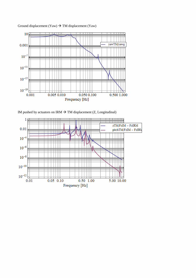
Ground displacement (Yaw) TM displacement (Yaw)

IM pushed by actuators on IRM TM displacement (Z, Longitudinal)