INL/EXT-15-36773

Light Water Reactor Sustainability Program

3D Simulation of External Flooding Events for the RISMC Pathway

September 2015

DOE Office of Nuclear Energy

DISCLAIMER This information was prepared as an account of work sponsored by an agency of the U.S. Government. Neither the U.S. Government nor any agency thereof, nor any of their employees, makes any warranty, expressed or implied, or assumes any legal liability or responsibility for the accuracy, completeness, or usefulness, of any information, apparatus, product, or process disclosed, or represents that its use would not infringe privately owned rights. References herein to any specific commercial product, process, or service by trade name, trade mark, manufacturer, or otherwise, do not necessarily constitute or imply its endorsement, recommendation, or favoring by the U.S. Government or any agency thereof. The views and opinions of authors expressed herein do not necessarily state or reflect those of the U.S. Government or any agency thereof.

INL/EXT-15-36773

Light Water Reactor Sustainability Program

3D Simulation of External Flooding Events for the RISMC Pathway

Steven Prescott, Diego Mandelli, Ramprasad Sampath, Curtis Smith, Linyu Lin

September 2015

Idaho National Laboratory Idaho Falls, Idaho 83415

http://www.inl.gov/lwrs

Prepared for the U.S. Department of Energy Office of Nuclear Energy

Under DOE Idaho Operations Office Contract DE-AC07-05ID14517

ii

ABSTRACT

Incorporating 3D simulations as part of the Risk-Informed Safety Margins Characterization (RISMIC) Toolkit allows analysts to obtain a more complete picture of complex system behavior for events including external plant hazards. External events such as flooding have become more important recently – however these can be analyzed with existing and validated simulated physics toolkits. In this report, we describe these approaches specific to flooding-based analysis using an approach called Smoothed Particle Hydrodynamics. The theory, validation, and example applications of the 3D flooding simulation are described. Integrating these 3D simulation methods into computational risk analysis provides a spatial/visual aspect to the design, improves the realism of results, and can prove visual understanding to validate the analysis of flooding.

iii

CONTENTS ABSTRACT .................................................................................................................................................. ii

FIGURES ..................................................................................................................................................... iv

TABLES ....................................................................................................................................................... v

ACRONYMS ............................................................................................................................................... vi

1. Introduction ........................................................................................................................................ 9

2. SPH Theory ...................................................................................................................................... 13

2.1 SPH Calculation Functions and Optimizations ................................................................... 14

2.1.1 Smoothing Kernels ............................................................................................ 14 2.1.2 Neighborhood Search ........................................................................................ 14 2.1.3 Approximating Fluid Equations of Motion ....................................................... 15 2.1.4 Calculating Density ........................................................................................... 16 2.1.5 Incompressible SPH .......................................................................................... 16 2.1.6 Boundary Handling ........................................................................................... 16

3. Validation of flooding models .......................................................................................................... 18

3.1 Dam Break Test ................................................................................................................... 18

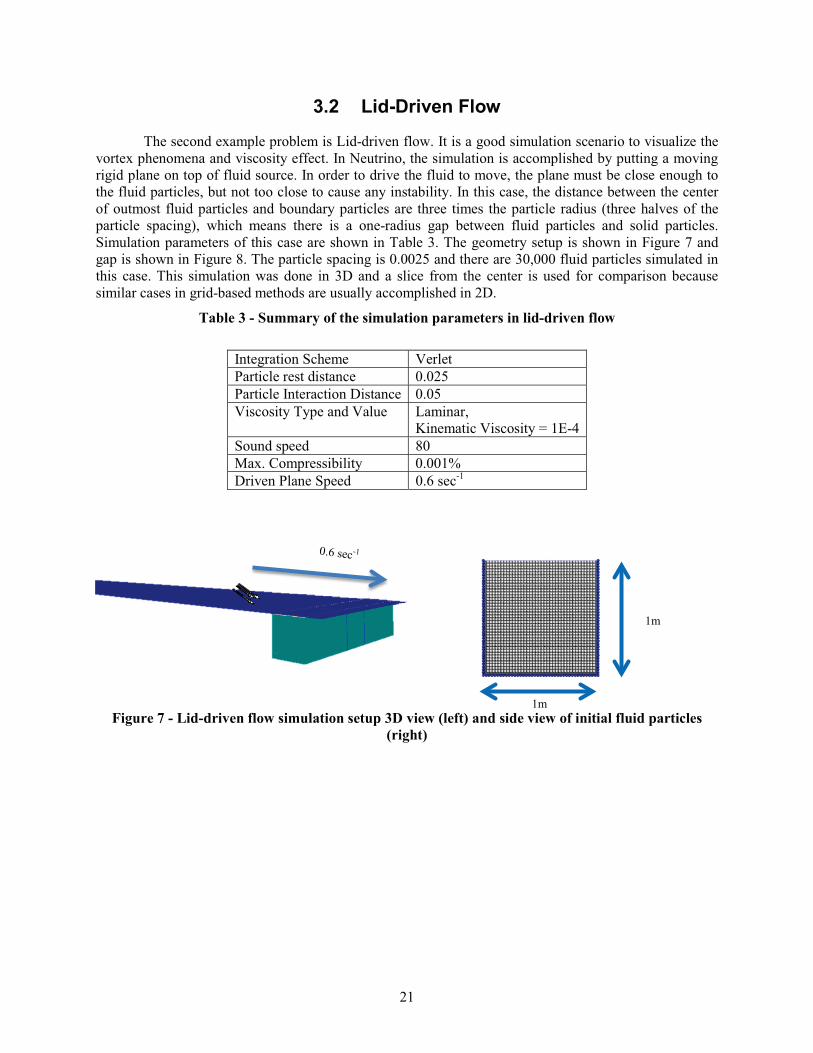
3.2 Lid-Driven Flow .................................................................................................................. 21

3.3 Vortex Shedding .................................................................................................................. 25

4. Plant damage metrics ........................................................................................................................ 27

5. Flooding Examples ........................................................................................................................... 30

5.1 Seawall analysis................................................................................................................... 30

5.2 Condensate Storage Tank .................................................................................................... 32

5.3 Power Grid Switch Yard ..................................................................................................... 34

5.4 Accessibility ........................................................................................................................ 35

6. Conclusions ...................................................................................................................................... 37

7. References ........................................................................................................................................ 38

iv

FIGURES

Figure 1 - Overview of the RISMC approach ............................................................................................. 10

Figure 2 – Multi-layer PRA approach within the RISMC Project .............................................................. 11

Figure 3 - Illustration of SPH approximation for a field variable of the red particle, where W denotes a Gaussian-like interpolation function (SPH kernel), h is the influence radius (smoothing length). .. 14

Figure 4 - Schematic diagram of the dam geometry [Cum12] .................................................................... 18

Figure 5 - Evolution of the water collapse and interaction with the column .............................................. 19

Figure 6 - Comparison of Neutrino output to experimental data ................................................................ 20

Figure 7 - Lid-driven flow simulation setup 3D view (left) and side view of initial fluid particles (right) 21

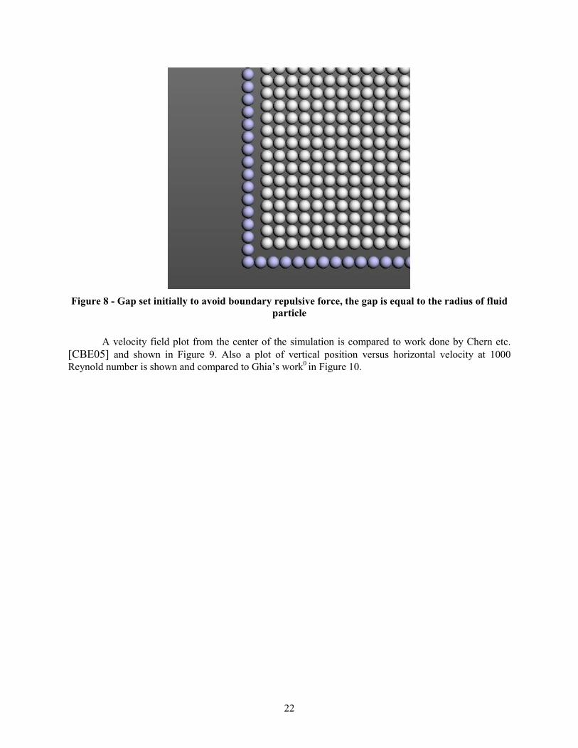
Figure 8 - Gap set initially to avoid boundary repulsive force, the gap is equal to the radius of fluid particle .............................................................................................................................................. 22

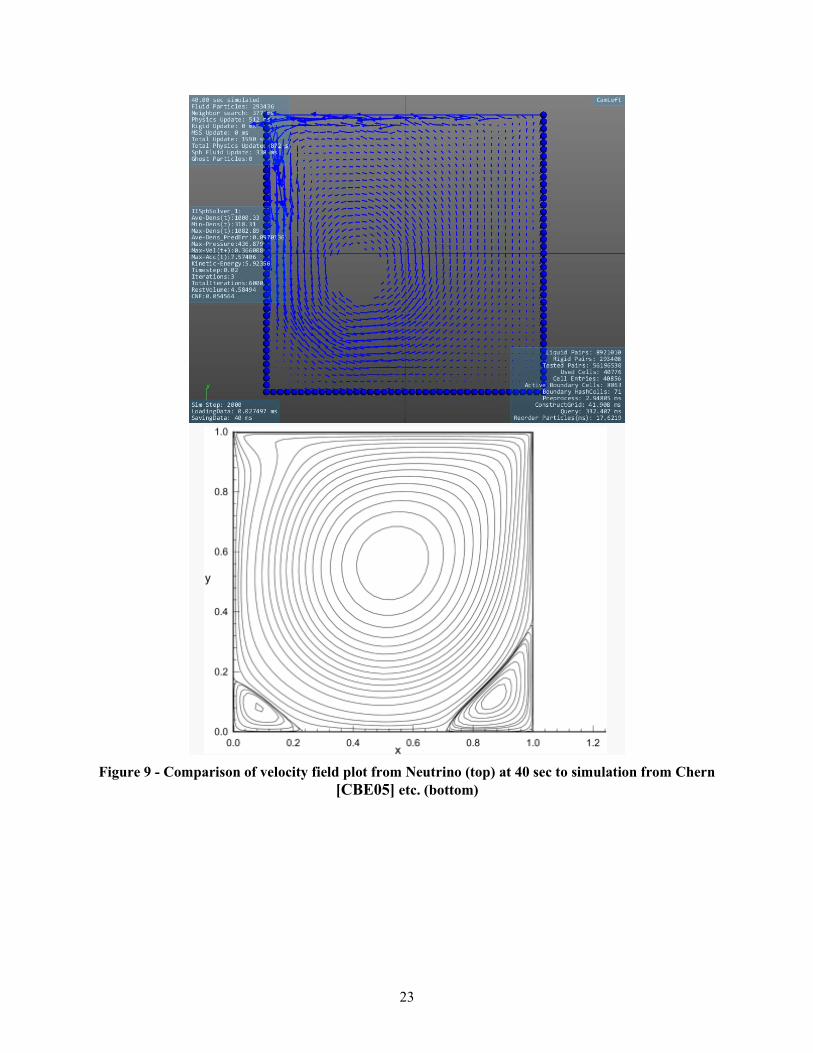
Figure 9 - Comparison of velocity field plot from Neutrino (top) at 40 sec to simulation from Chern [CBE05] etc. (bottom) ...................................................................................................................... 23

Figure 10 - Plot of vertical position versus horizontal velocity at middle line compared to Ghia’s data [Ghi82]. ............................................................................................................................................ 24

Figure 11 - Comparison of particle profile at middle of the box after 20 sec simulation with artificial viscosity (top, no spinning or vortex formed) again profile with laminar viscosity with equivalent viscosity value (bottom, spinning and vortex hole) .......................................................................... 25

Figure 12 - Vortex shedding after flow pass cylinder from Neutrino (top) and from Giosan (bottom) ..... 26

Figure 13 - Representation as even-tree structure of the RAVEN/RELAP-7 simulation. Note that the parameter characterizing the initiating event, i.e. wave height, affects timing of the event-tree branches (e.g., recovery time for PG) ............................................................................................... 27

Figure 14 - Max flooding levels for several wave heights. ......................................................................... 28

Figure 15 – Extended flooding event-tree ................................................................................................... 29

Figure 16 – Seawall modification analysis for a tsunami several meters over seawall height. .................. 31

Figure 17 – Seawall modification analysis for a tsunami slightly over seawall height .............................. 32

Figure 18 - The impact force being measured on the Condensate Storage Tank ........................................ 33

Figure 19 - Total force on the tank from two scenarios. ............................................................................. 34

Figure 20 – Off-site power grid switchyard location and flooding status for a 15m wave ......................... 35

Figure 21 – 3D simulation estimating the movement of debris (left). Interior flooding can impact human accessibility (right). .......................................................................................................................... 36

v

TABLES

Table 1 - Summary of the simulation parameters in dam break case ......................................................... 19

Table 2 - Comparison of experimental measurement, neutrino, LAMMPS-SPH and Dual-SPHysics ...... 20

Table 3 - Summary of the simulation parameters in lid-driven flow .......................................................... 21

vi

ACRONYMS

AC Alternating Current

ADS Automatic Depressurization System

BWR Boiling Water Reactor

CDF Cumulative Distribution Function

CRA Computational Risk Assessment

DOE Department of Energy

DG Diesel generator

DW Drywell

EOP Emergency Operating Procedures

ET Event-Tree

FT Fault-Tree

FW Firewater

HPCI High Pressure Core Injection

IE Initiating Event

INL Idaho National Laboratory

LOOP Loss Of Offsite Power

LWR Light Water Reactor

LWRS Light Water Reactor Sustainability

MOOSE Multi-physics Object-Oriented Simulation Environment

NPP Nuclear Power Plant

PDF Probability Distribution Function

PG Power Grid

PRA Probabilistic Risk Assessment

PSP Pressure Suppression Pool

vii

PWR Pressurized Water Reactor

R&D Research and Development

RCIC Reactor Core Isolation Cooling

RISMC Risk Informed Safety Margin Characterization

T-H Thermal-Hydraulics

9

3D Simulation of External Flooding Events for the RISMC Pathway

1. Introduction

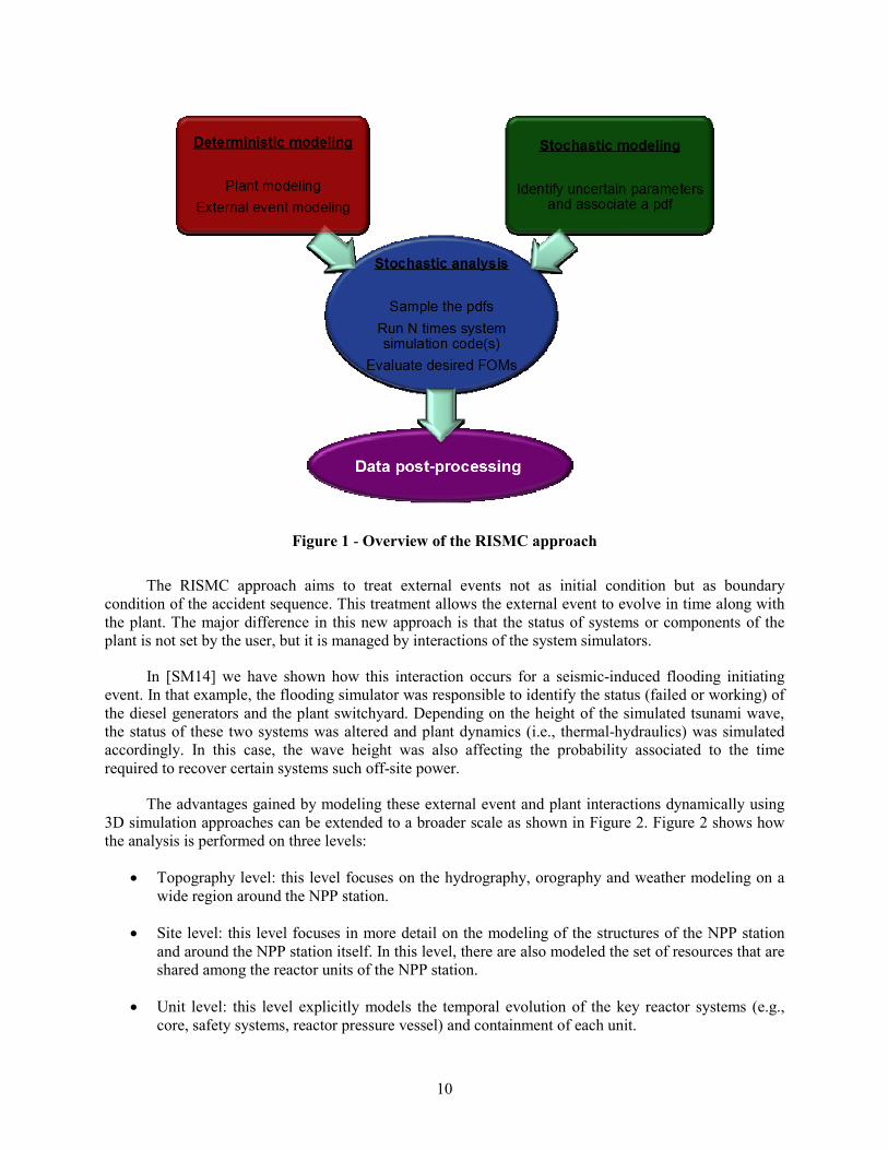
The Risk-Informed Safety Margins Characterization (RISMC) Pathway [SRM11] uses probabilistic methods to determine safety margins and to quantify their impacts on reliability and safety for existing Nuclear Power Plants (NPPs), i.e., pressurized and boiling water reactors (PWRs and BWRs). As part of the quantification, we use both probabilistic (via risk simulation) and mechanistic (via system simulators) approaches (see Figure 1). In the plant simulation, all the deterministic aspects that characterize system dynamics (e.g., thermal-hydraulic, thermal-mechanics, neutronics) are coupled to each other.

For the deterministic side we include:

• Modeling of thermal-hydraulic behavior of plant

• Modeling of external events such as flooding

• Modeling of the operators’ responses to the accident scenario

Note that deterministic modeling of plant or external events can be performed by employing specific simulator codes or by surrogate models, known as reduced order models (ROM). ROMs would be employed in order to decrease the high computational costs of employed codes where applicable.

In addition, multi-fidelity codes can be used to model a system where we have the ability to switch from a low-fidelity to high-fidelity code (or selectable fidelity of the same code if it has that capability) when higher accuracy is needed (e.g., use low-fidelity codes for steady-state conditions and high-fidelity code for transient conditions).

On the other hand, in the stochastic modeling, we include all stochastic parameters that are of interest in the probabilistic assessment such as:

• Uncertain parameters

• Stochastic failure of system/components/humans

In this report we focus on the deterministic modeling of external events and in particular flooding related events. In [SM14] we showed the feasibility of an analysis that couples an external event simulation code (i.e., the NEUTRINO flooding code) and a plant system simulation code (i.e., RELAP-7). That analysis shows not only the feasibility of this coupling but, more important, how external events are modeled in the RISMC approach. In classical probabilistic risk assessment (PRA) approaches, external events are loosely considered in the analysis, i.e., they are treated as initial conditions for the analysis: for example, the status of few systems or components (e.g., off-site power is unavailable at the beginning of a SBO analysis) is typically set before the PRA analysis is performed by the user.

10

Figure 1 - Overview of the RISMC approach

The RISMC approach aims to treat external events not as initial condition but as boundary condition of the accident sequence. This treatment allows the external event to evolve in time along with the plant. The major difference in this new approach is that the status of systems or components of the plant is not set by the user, but it is managed by interactions of the system simulators.

In [SM14] we have shown how this interaction occurs for a seismic-induced flooding initiating event. In that example, the flooding simulator was responsible to identify the status (failed or working) of the diesel generators and the plant switchyard. Depending on the height of the simulated tsunami wave, the status of these two systems was altered and plant dynamics (i.e., thermal-hydraulics) was simulated accordingly. In this case, the wave height was also affecting the probability associated to the time required to recover certain systems such off-site power.

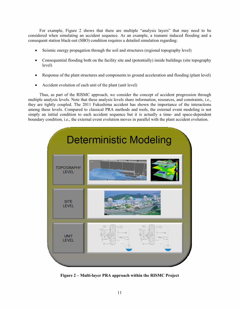
The advantages gained by modeling these external event and plant interactions dynamically using 3D simulation approaches can be extended to a broader scale as shown in Figure 2. Figure 2 shows how the analysis is performed on three levels:

• Topography level: this level focuses on the hydrography, orography and weather modeling on a wide region around the NPP station.

• Site level: this level focuses in more detail on the modeling of the structures of the NPP station and around the NPP station itself. In this level, there are also modeled the set of resources that are shared among the reactor units of the NPP station.

• Unit level: this level explicitly models the temporal evolution of the key reactor systems (e.g., core, safety systems, reactor pressure vessel) and containment of each unit.

11

For example, Figure 2 shows that there are multiple “analysis layers” that may need to be considered when simulating an accident sequence. As an example, a tsunami induced flooding and a consequent station black-out (SBO) condition requires a detailed simulation regarding:

• Seismic energy propagation through the soil and structures (regional topography level)

• Consequential flooding both on the facility site and (potentially) inside buildings (site topography level)

• Response of the plant structures and components to ground acceleration and flooding (plant level)

• Accident evolution of each unit of the plant (unit level)

Thus, as part of the RISMC approach, we consider the concept of accident progression through multiple analysis levels. Note that these analysis levels share information, resources, and constraints, i.e., they are tightly coupled. The 2011 Fukushima accident has shown the importance of the interactions among these levels. Compared to classical PRA methods and tools, the external event modeling is not simply an initial condition to each accident sequence but it is actually a time- and space-dependent boundary condition, i.e., the external event evolution moves in parallel with the plant accident evolution.

Figure 2 – Multi-layer PRA approach within the RISMC Project

12

This report also shows some of the advantages to perform risk assessments for complex systems using computational risk assessment (CRA) methods (i.e., RISMC) compared to the PRA analyses performed with classical methods based on event-tree (ET) and fault-tree (FT) static logic structures. We have identified four possible correlation factors that would require the need of CRA methods:

1. Time: correlations of timing and sequencing of events

2. Space: correlations between the spatial location of components and systems

3. Physics: correlations between physical phenomena that might evolve on different spatial (from nano-meters to meters) and temporal scale (from micro-seconds to years)

4. Complexity: correlation due to information sharing between plant systems, components and humans

In this report we will focus to show how all these four factors can be modeled by using the RISMC approach.

13

2. SPH Theory

3D animation is the movement of objects in space over a period of time; 3D simulation adds defined physical interactions between those objects. These physical interactions can be done in varying degrees and use a wide range of methods, algorithms, and fidelity. Using more advanced methods, we can mimic natural events with substantial accuracy. One of these methods of representing fluids and other interactions is known as Smoothed Particle Hydrodynamics (SPH). It is a common and viable method for simulating 3D fluid and rigid body interactions, and the use of incompressible flow of particle-based techniques has advanced it even further. SPH has important potential benefits, such as the ability to handle complex boundaries and small-scale phenomena. While there are some codes available for SPH-based simulation of large geophysical domains [Cre11], for our simulations, we use SPH for large scale domain using a parallelized Implicit Incompressible SPH method.

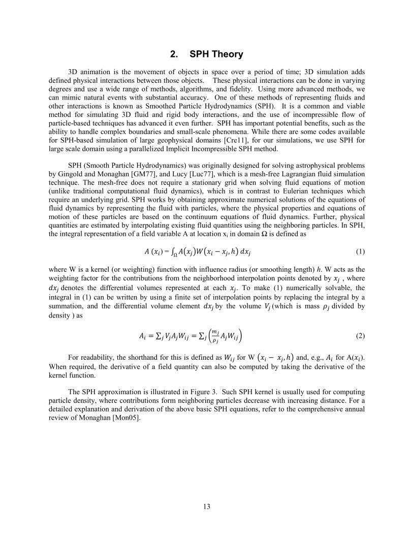
SPH (Smooth Particle Hydrodynamics) was originally designed for solving astrophysical problems by Gingold and Monaghan [GM77], and Lucy [Luc77], which is a mesh-free Lagrangian fluid simulation technique. The mesh-free does not require a stationary grid when solving fluid equations of motion (unlike traditional computational fluid dynamics), which is in contrast to Eulerian techniques which require an underlying grid. SPH works by obtaining approximate numerical solutions of the equations of fluid dynamics by representing the fluid with particles, where the physical properties and equations of motion of these particles are based on the continuum equations of fluid dynamics. Further, physical quantities are estimated by interpolating existing fluid quantities using the neighboring particles. In SPH, the integral representation of a field variable A at location xi in domain Ω is defined as

𝐴𝐴 (𝑥𝑥𝑖𝑖) = ∫ 𝐴𝐴𝑥𝑥𝑗𝑗𝑊𝑊𝑥𝑥𝑖𝑖 − 𝑥𝑥𝑗𝑗,ℎ 𝑑𝑑𝑥𝑥𝑗𝑗 Ω (1)

where W is a kernel (or weighting) function with influence radius (or smoothing length) h. W acts as the weighting factor for the contributions from the neighborhood interpolation points denoted by 𝑥𝑥𝑗𝑗 , where 𝑑𝑑𝑥𝑥𝑗𝑗 denotes the differential volumes represented at each 𝑥𝑥𝑗𝑗. To make (1) numerically solvable, the integral in (1) can be written by using a finite set of interpolation points by replacing the integral by a summation, and the differential volume element 𝑑𝑑𝑥𝑥𝑗𝑗 by the volume 𝑉𝑉𝑗𝑗 (which is mass 𝜌𝜌𝑗𝑗 divided by density ) as

𝐴𝐴𝑖𝑖 = ∑ 𝑉𝑉𝑗𝑗𝐴𝐴𝑗𝑗𝑊𝑊𝑖𝑖𝑗𝑗 = ∑ 𝑚𝑚𝑗𝑗

𝜌𝜌𝑗𝑗𝐴𝐴𝑗𝑗𝑊𝑊𝑖𝑖𝑗𝑗𝑗𝑗𝑗𝑗 (2)

For readability, the shorthand for this is defined as 𝑊𝑊𝑖𝑖𝑗𝑗 for W 𝑥𝑥𝑖𝑖 − 𝑥𝑥𝑗𝑗,ℎ and, e.g., 𝐴𝐴𝑖𝑖 for A(𝑥𝑥𝑖𝑖). When required, the derivative of a field quantity can also be computed by taking the derivative of the kernel function.

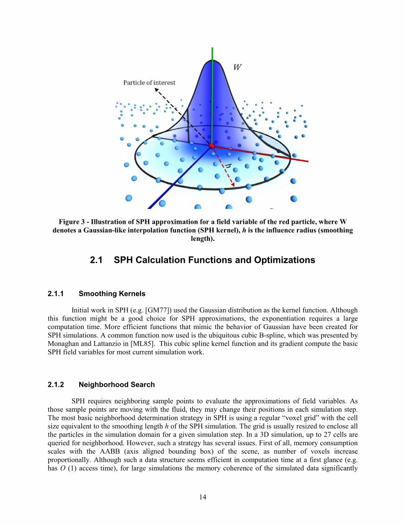
The SPH approximation is illustrated in Figure 3. Such SPH kernel is usually used for computing particle density, where contributions form neighboring particles decrease with increasing distance. For a detailed explanation and derivation of the above basic SPH equations, refer to the comprehensive annual review of Monaghan [Mon05].

14

Figure 3 - Illustration of SPH approximation for a field variable of the red particle, where W denotes a Gaussian-like interpolation function (SPH kernel), h is the influence radius (smoothing

length).

2.1 SPH Calculation Functions and Optimizations

2.1.1 Smoothing Kernels

Initial work in SPH (e.g. [GM77]) used the Gaussian distribution as the kernel function. Although this function might be a good choice for SPH approximations, the exponentiation requires a large computation time. More efficient functions that mimic the behavior of Gaussian have been created for SPH simulations. A common function now used is the ubiquitous cubic B-spline, which was presented by Monaghan and Lattanzio in [ML85]. This cubic spline kernel function and its gradient compute the basic SPH field variables for most current simulation work.

2.1.2 Neighborhood Search

SPH requires neighboring sample points to evaluate the approximations of field variables. As those sample points are moving with the fluid, they may change their positions in each simulation step. The most basic neighborhood determination strategy in SPH is using a regular “voxel grid” with the cell size equivalent to the smoothing length h of the SPH simulation. The grid is usually resized to enclose all the particles in the simulation domain for a given simulation step. In a 3D simulation, up to 27 cells are queried for neighborhood. However, such a strategy has several issues. First of all, memory consumption scales with the AABB (axis aligned bounding box) of the scene, as number of voxels increase proportionally. Although such a data structure seems efficient in computation time at a first glance (e.g. has O (1) access time), for large simulations the memory coherence of the simulated data significantly

15

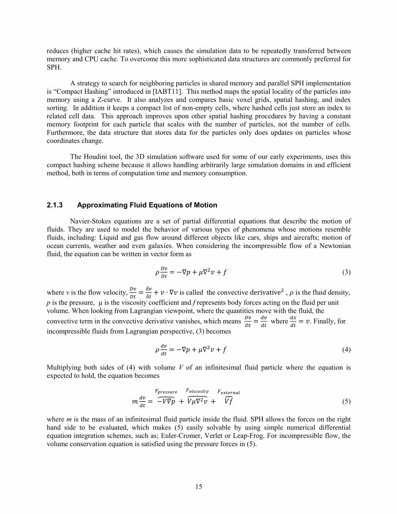
reduces (higher cache hit rates), which causes the simulation data to be repeatedly transferred between memory and CPU cache. To overcome this more sophisticated data structures are commonly preferred for SPH.

A strategy to search for neighboring particles in shared memory and parallel SPH implementation is “Compact Hashing” introduced in [IABT11]. This method maps the spatial locality of the particles into memory using a Z-curve. It also analyzes and compares basic voxel grids, spatial hashing, and index sorting. In addition it keeps a compact list of non-empty cells, where hashed cells just store an index to related cell data. This approach improves upon other spatial hashing procedures by having a constant memory footprint for each particle that scales with the number of particles, not the number of cells. Furthermore, the data structure that stores data for the particles only does updates on particles whose coordinates change.

The Houdini tool, the 3D simulation software used for some of our early experiments, uses this compact hashing scheme because it allows handling arbitrarily large simulation domains in and efficient method, both in terms of computation time and memory consumption.

2.1.3 Approximating Fluid Equations of Motion

Navier-Stokes equations are a set of partial differential equations that describe the motion of fluids. They are used to model the behavior of various types of phenomena whose motions resemble fluids, including: Liquid and gas flow around different objects like cars, ships and aircrafts; motion of ocean currents, weather and even galaxies. When considering the incompressible flow of a Newtonian fluid, the equation can be written in vector form as

𝜌𝜌 𝐷𝐷𝐷𝐷𝐷𝐷𝐷𝐷

= −∇𝑝𝑝 + 𝜇𝜇∇2𝑣𝑣 + 𝑓𝑓 (3)

where v is the flow velocity, 𝐷𝐷𝐷𝐷𝐷𝐷𝐷𝐷

= 𝛿𝛿𝐷𝐷𝛿𝛿𝐷𝐷

+ 𝑣𝑣 ∙ ∇𝑣𝑣 is called the convective derivative2 , 𝜌𝜌 is the fluid density, p is the pressure, µ is the viscosity coefficient and f represents body forces acting on the fluid per unit volume. When looking from Lagrangian viewpoint, where the quantities move with the fluid, the convective term in the convective derivative vanishes, which means 𝐷𝐷𝐷𝐷

𝐷𝐷𝐷𝐷= 𝑑𝑑𝐷𝐷

𝑑𝑑𝐷𝐷 where 𝑑𝑑𝑑𝑑

𝑑𝑑𝐷𝐷= 𝑣𝑣. Finally, for

incompressible fluids from Lagrangian perspective, (3) becomes

𝜌𝜌 𝑑𝑑𝐷𝐷𝑑𝑑𝐷𝐷

= −∇𝑝𝑝 + 𝜇𝜇∇2𝑣𝑣 + 𝑓𝑓 (4)

Multiplying both sides of (4) with volume V of an infinitesimal fluid particle where the equation is expected to hold, the equation becomes

𝑚𝑚𝑑𝑑𝐷𝐷𝑑𝑑𝐷𝐷

= −𝑉𝑉𝛻𝛻𝑝𝑝𝐹𝐹𝑝𝑝𝑝𝑝𝑝𝑝𝑝𝑝𝑝𝑝𝑝𝑝𝑝𝑝𝑝𝑝

+ 𝑉𝑉𝜇𝜇∇2𝑣𝑣𝐹𝐹𝑣𝑣𝑣𝑣𝑝𝑝𝑣𝑣𝑣𝑣𝑝𝑝𝑣𝑣𝑣𝑣𝑣𝑣

+ 𝑉𝑉𝑓𝑓𝐹𝐹𝑝𝑝𝑒𝑒𝑣𝑣𝑝𝑝𝑝𝑝𝑛𝑛𝑛𝑛𝑛𝑛

(5)

where m is the mass of an infinitesimal fluid particle inside the fluid. SPH allows the forces on the right hand side to be evaluated, which makes (5) easily solvable by using simple numerical differential equation integration schemes, such as; Euler-Cromer, Verlet or Leap-Frog. For incompressible flow, the volume conservation equation is satisfied using the pressure forces in (5).

16

2.1.4 Calculating Density

Since the pressure force arises as a result of the changes in the fluid density it is the most important field variable of SPH simulations. A well-known way to compute fluid density in SPH is using the summation density approach [Mon05]. It can be easily derived from the basic SPH scheme by substituting fluid density 𝜌𝜌 as the field variable A into (2), which results in

𝜌𝜌𝑖𝑖 = ∑ 𝑚𝑚𝑗𝑗𝑊𝑊𝑖𝑖𝑗𝑗𝑗𝑗 . (6)

The most important issue with the summation density technique is that it results in underestimated density values near fluid interfaces. Reconstruction the density field as correctly as possible is very crucial in SPH, since pressure force that is to satisfy incompressibility solely relies on the density field.

Another way to update density is to use the mass continuity equation

𝐷𝐷𝜌𝜌𝐷𝐷𝐷𝐷

+ ρ(∇ ∙ 𝑣𝑣) = 0 (7)

as a basis. Expanding the convective derivative and leaving the time rate of change of density and approximating 𝐷𝐷𝜌𝜌

𝐷𝐷𝐷𝐷 using SPH results in

𝑑𝑑𝜌𝜌𝑣𝑣𝑑𝑑𝐷𝐷

= ∑ 𝑚𝑚𝑗𝑗(𝑣𝑣𝑖𝑖 − 𝑣𝑣𝑗𝑗) ∙ ∇𝑊𝑊𝑖𝑖𝑗𝑗𝑗𝑗 (8)

where the rate of change of density is computed based on the relative motion of the particles [Mon92]. (8) has computational advantage over (7), as all field variables that are necessary to solve fluid equations of motion can be computed in a single loop over the particles. Although (8) looks as if it is unaffected by the underestimated densities near fluid interfaces, it has different issues. First of all, the accumulation of numerical errors, and the errors caused by time integration schemes cause stability issues. The common practice to alleviate these problems is to reinitialize the particles’ densities time to a time using (7), and using a density correction strategy. One of the most common correction strategies is to use Shepard filter [She68] as done in [Pan04]. Another strategy is to use Moving Least Squares (MLS) technique as used in [Pan04].

2.1.5 Incompressible SPH

Ihmsen et al. [ICS+13] proposed a technique that uses an SPH approximation of the continuity equation to obtain a discretized form of pressure Poisson equation. They call the technique Implicit Incompressible SPH (IISPH). Different from the previous projection-based techniques, IISPH also considers the actual computation of the pressure force, which improves the convergence rate of the solver. Additionally, the density deviation in IISPH is computed based on particle velocities instead of positions, which improves the robustness of the solver.

2.1.6 Boundary Handling

The Houdini simulation software uses a versatile method for the two-way coupling of SPH fluids and rigid bodies. Boundary particles are used to sample the surface of rigid objects, which has several benefits. First, the use of particles gives the ability to derive a model that can cope with different shapes,

17

including lower-dimensional rigid bodies consisting of one layer (referred to as thin shells) or one line of boundary particles (referred to as rods), as well as non-manifold geometries. Second, the inclusion of boundary particles successfully alleviates the particle deficiency problem of SPH near boundaries, preventing density (and consequently pressure) discontinuities at the boundary and particle sticking artifacts.

This model addresses the problem of inhomogeneous particle sampling at the boundary by deriving new equations that consider the relative contribution of a boundary particle to a physical quantity. This does not only facilitate the particle initialization at complex boundaries, but also enables the use of multiple dynamic objects where the boundary sampling in the neighborhood may change due to contacts. A friction model is additionally included to simulate various slip conditions and drag effects. All pressure and viscous forces that are applied between fluid and boundary particles are symmetric, conserving linear and angular momentum. The approach is designed such that even very large density ratios between fluids and rigid bodies can be handled.

Since the focus is on the interaction of fluids with non-deformable rigid bodies without melting effects, particles do not necessarily need to be generated inside a rigid. Therefore, particles are generated as a single layer at the surface similar to [BYM05]. This approach saves memory and improves performance. The particle representations of rigid bodies in the framework are computed either directly (e.g. for analytical shapes) or from mesh representations. Particle representations of triangle meshes are generated based on [BYM05], which permits placing particles at an arbitrary offset to the surface mesh and yields a quite homogenous sampling. However, at regions with high-curvature, the particle distribution usually remains non-homogenous, resulting in a denser sampling in such areas. Details of the boundary handling can be found in [NA12].

18

3. Validation of flooding models

Being able to virtually run a scenario provided useful risk information and makes it possible to understand plant behavior prior to seeing actual events such as floods. However, we need to be assured that these simulations can deliver valid and practical results. Initial validation tests have begun for the Neutrino simulation software being used in our external event analysis. Testing against real world data and other simulation methods has been performed and are described in this section.

3.1 Dam Break Test

The dam break scenario is a typical test case done to validate movement and forces. It is

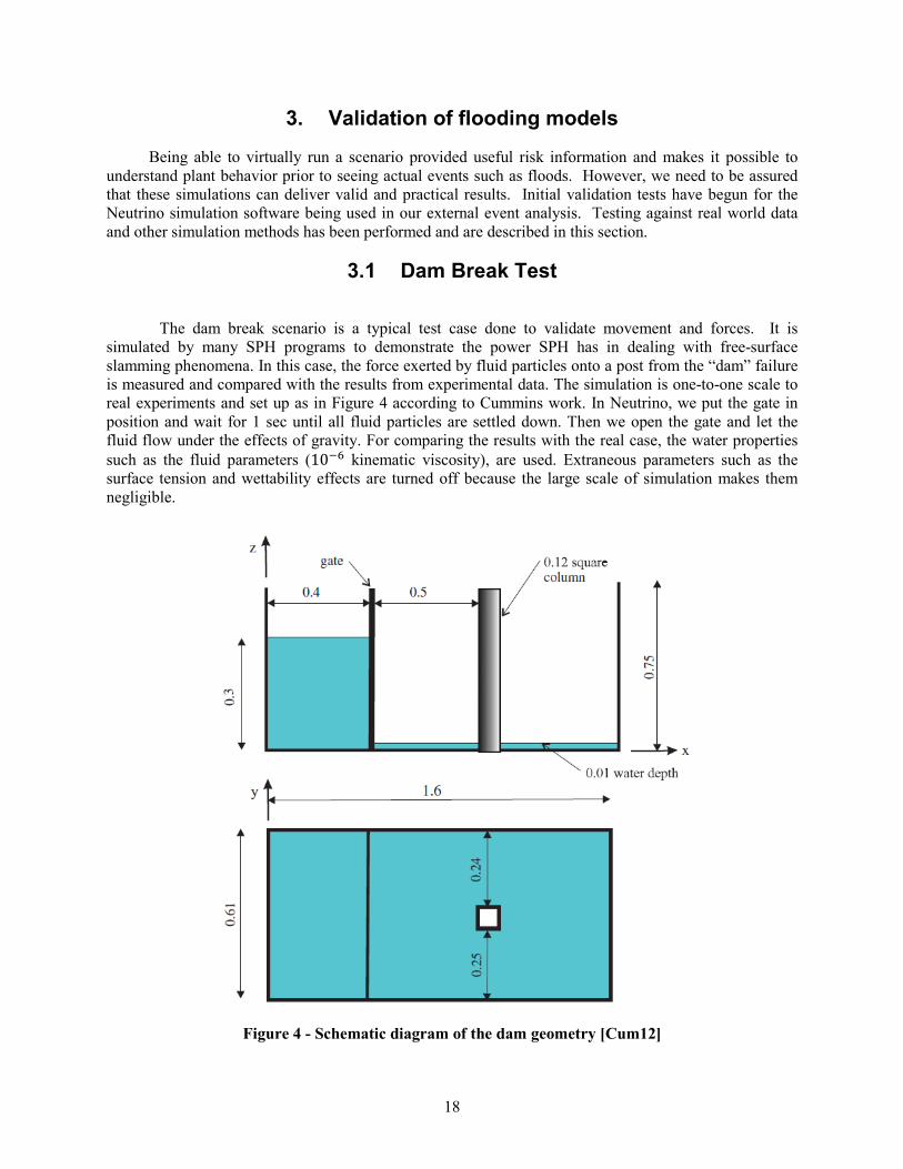
simulated by many SPH programs to demonstrate the power SPH has in dealing with free-surface slamming phenomena. In this case, the force exerted by fluid particles onto a post from the “dam” failure is measured and compared with the results from experimental data. The simulation is one-to-one scale to real experiments and set up as in Figure 4 according to Cummins work. In Neutrino, we put the gate in position and wait for 1 sec until all fluid particles are settled down. Then we open the gate and let the fluid flow under the effects of gravity. For comparing the results with the real case, the water properties such as the fluid parameters (10−6 kinematic viscosity), are used. Extraneous parameters such as the surface tension and wettability effects are turned off because the large scale of simulation makes them negligible.

Figure 4 - Schematic diagram of the dam geometry [Cum12]

19

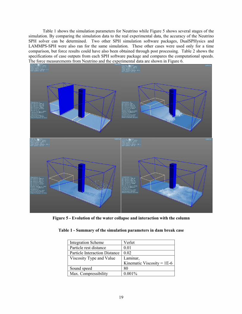
Table 1 shows the simulation parameters for Neutrino while Figure 5 shows several stages of the simulation. By comparing the simulation data to the real experimental data, the accuracy of the Neutrino SPH solver can be determined. Two other SPH simulation software packages, DualSPHysics and LAMMPS-SPH were also ran for the same simulation. These other cases were used only for a time comparison, but force results could have also been obtained through post processing. Table 2 shows the specifications of case outputs from each SPH software package and compares the computational speeds. The force measurements from Neutrino and the experimental data are shown in Figure 6.

Figure 5 - Evolution of the water collapse and interaction with the column

Table 1 - Summary of the simulation parameters in dam break case

Integration Scheme Verlet Particle rest distance 0.01 Particle Interaction Distance 0.02 Viscosity Type and Value Laminar,

Kinematic Viscosity = 1E-6 Sound speed 80 Max. Compressibility 0.001%

20

Table 2 - Comparison of experimental measurement, neutrino, LAMMPS-SPH and Dual-SPHysics

Force Measurement

Total Particle #

CPU time per simulation step (sec/step)

Avg. unit Time Step Size (sec)

Experimental Data

Yes

Neutrino Yes 67053 0.057 (4 cores 2.7 Ghz) 0.00102 LAMMPS-SPH Needs

post-processing 64906 0.136 (8 cores 2.7 Ghz) 0.00087

DualSPHysics Needs post-processing

116795 1.454 (4 cores 2.7 Ghz) 0.0004

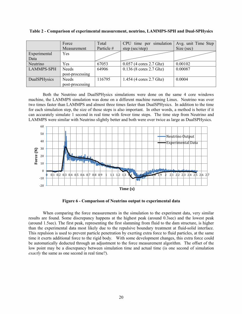
Both the Neutrino and DualSPHysics simulations were done on the same 4 core windows machine, the LAMMPS simulation was done on a different machine running Linux. Neutrino was over two times faster than LAMMPS and almost three times faster than DualSPHysics. In addition to the time for each simulation step, the size of those steps is also important. In other words, a method is better if it can accurately simulate 1 second in real time with fewer time steps. The time step from Neutrino and LAMMPS were similar with Neutrino slightly better and both were over twice as large as DualSPHysics.

Figure 6 - Comparison of Neutrino output to experimental data

When comparing the force measurements in the simulation to the experiment data, very similar results are found. Some discrepancy happens at the highest peak (around 0.3sec) and the lowest peak (around 1.5sec). The first peak, representing the first slamming from fluid to the dam structure, is higher than the experimental data most likely due to the repulsive boundary treatment at fluid-solid interface. This repulsion is used to prevent particle penetration by exerting extra force to fluid particles, at the same time it exerts additional force to the rigid body. With some development changes, this extra force could be automatically deducted through an adjustment to the force measurement algorithm. The offset of the low point may be a discrepancy between simulation time and actual time (is one second of simulation exactly the same as one second in real time?).

-20

-10

0

10

20

30

40

50

60

0 0.1 0.2 0.3 0.4 0.5 0.6 0.7 0.8 0.9 1 1.1 1.2 1.3 1.4 1.5 1.6 1.7 1.8 1.9 2 2.1 2.2 2.3 2.4 2.5 2.6 2.7

Forc

e (N

)

Time (s)

Neutrino OutputExperimental Data

22

Figure 8 - Gap set initially to avoid boundary repulsive force, the gap is equal to the radius of fluid

particle

A velocity field plot from the center of the simulation is compared to work done by Chern etc. [CBE05] and shown in Figure 9. Also a plot of vertical position versus horizontal velocity at 1000 Reynold number is shown and compared to Ghia’s work0 in Figure 10.

23

Figure 9 - Comparison of velocity field plot from Neutrino (top) at 40 sec to simulation from Chern

[CBE05] etc. (bottom)

24

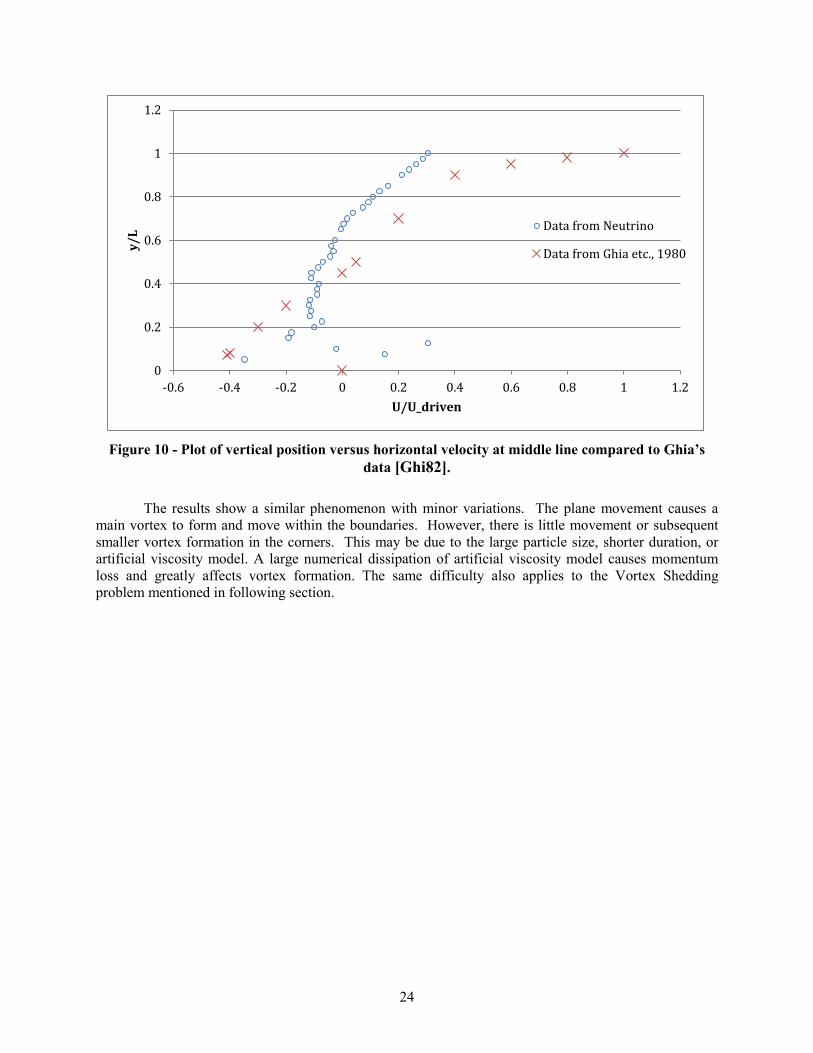
Figure 10 - Plot of vertical position versus horizontal velocity at middle line compared to Ghia’s

data [Ghi82].

The results show a similar phenomenon with minor variations. The plane movement causes a main vortex to form and move within the boundaries. However, there is little movement or subsequent smaller vortex formation in the corners. This may be due to the large particle size, shorter duration, or artificial viscosity model. A large numerical dissipation of artificial viscosity model causes momentum loss and greatly affects vortex formation. The same difficulty also applies to the Vortex Shedding problem mentioned in following section.

0

0.2

0.4

0.6

0.8

1

1.2

-0.6 -0.4 -0.2 0 0.2 0.4 0.6 0.8 1 1.2

y/L

U/U_driven

Data from Neutrino

Data from Ghia etc., 1980

25

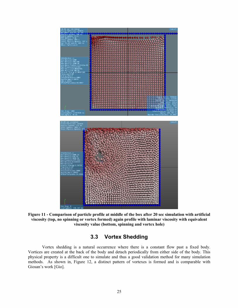
Figure 11 - Comparison of particle profile at middle of the box after 20 sec simulation with artificial

viscosity (top, no spinning or vortex formed) again profile with laminar viscosity with equivalent viscosity value (bottom, spinning and vortex hole)

3.3 Vortex Shedding

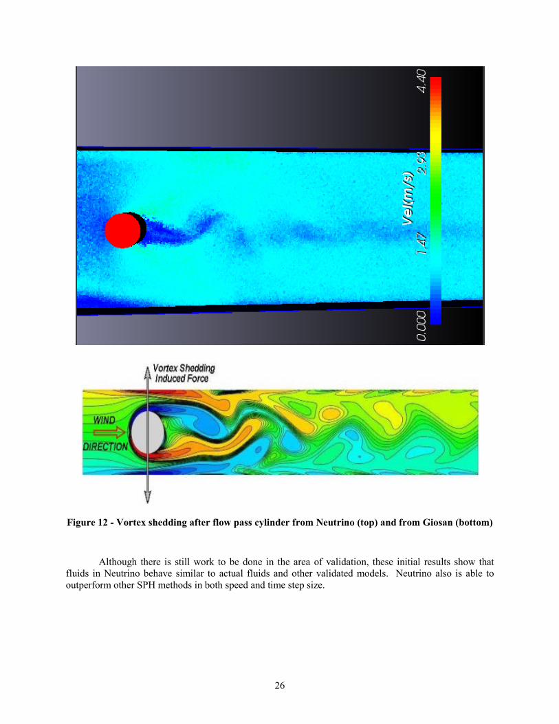
Vortex shedding is a natural occurrence where there is a constant flow past a fixed body. Vortices are created at the back of the body and detach periodically from either side of the body. This physical property is a difficult one to simulate and thus a good validation method for many simulation methods. As shown in, Figure 12, a distinct pattern of vortexes is formed and is comparable with Giosan’s work [Gio].

26

Figure 12 - Vortex shedding after flow pass cylinder from Neutrino (top) and from Giosan (bottom)

Although there is still work to be done in the area of validation, these initial results show that fluids in Neutrino behave similar to actual fluids and other validated models. Neutrino also is able to outperform other SPH methods in both speed and time step size.

27

4. Plant damage metrics

To account for the complexity of realistic events, the evolution of the flooding event is running in parallel with the plant accident scenario. This allows the user to perform an analysis that tightly couples plant and flooding dynamics. This coupling is made when the status of set of systems or components is monitored and updated throughout the simulation such as:

• Off-site power grid switchyard

• Diesel generators building

• Accessibility

• Condensate storage tanks

Figure 13 - Representation as even-tree structure of the RAVEN/RELAP-7 simulation. Note that the parameter characterizing the initiating event, i.e. wave height, affects timing of the event-tree

branches (e.g., recovery time for PG)

In [SM14] we have shown an example of flooding-plant dynamics interaction for a simplified case of PWR SBO test case where we monitored the status of the diesel generator building and the off-site power grid switchyard. In Figure 13 we have shown this interaction by using an event-tree diagram. For each branch multiple simulations are run where timing and ordering of events are randomly changed accordingly to a specific set of probabilistic distribution functions. Depending on the wave height that causes the plant flooding:

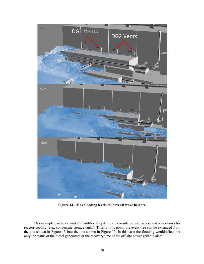
• Diesel generator may be taken out of service due to water infiltration inside their building (see Figure 14)

• Off-site power grid switchyard may be flooded and this would directly affects its recovery time

28

Figure 14 - Max flooding levels for several wave heights.

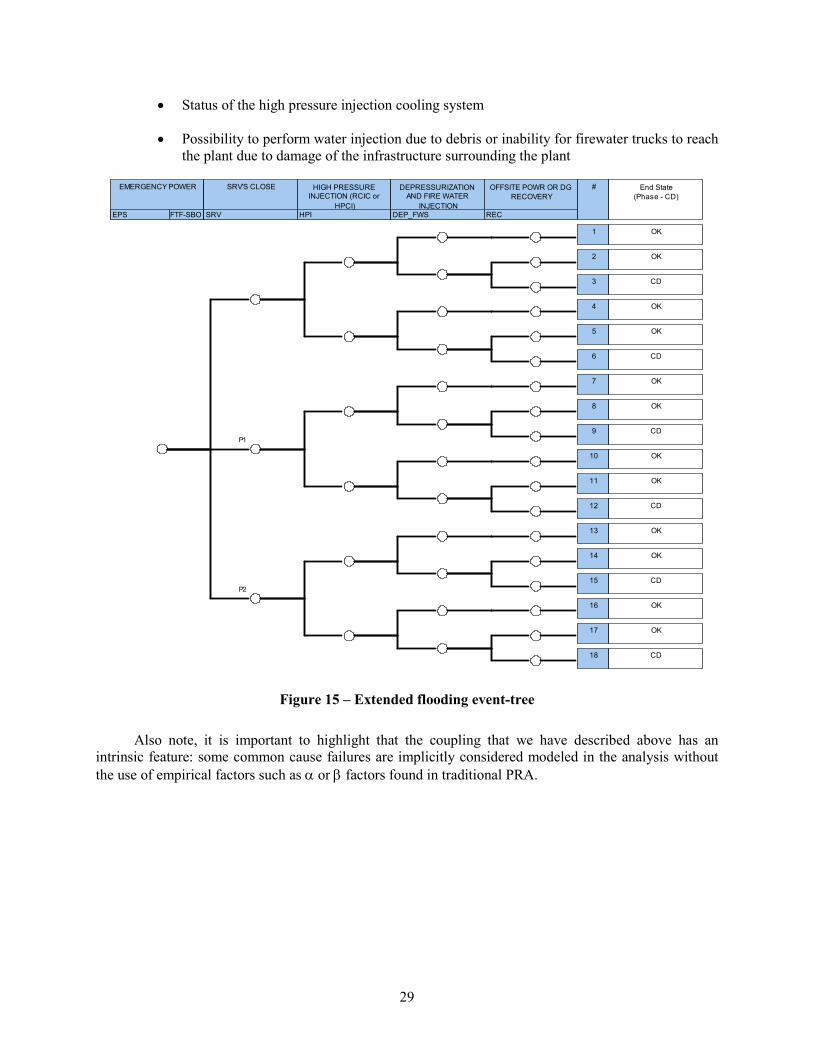
This example can be expanded if additional systems are considered: site access and water tanks for reactor cooling (e.g., condensate storage tanks). Thus, at this point, the event-tree can be expanded from the one shown in Figure 13 into the one shown in Figure 15. In this case the flooding would affect not only the status of the diesel generators or the recovery time of the off-site power grid but also:

29

• Status of the high pressure injection cooling system

• Possibility to perform water injection due to debris or inability for firewater trucks to reach the plant due to damage of the infrastructure surrounding the plant

Figure 15 – Extended flooding event-tree

Also note, it is important to highlight that the coupling that we have described above has an intrinsic feature: some common cause failures are implicitly considered modeled in the analysis without the use of empirical factors such as α or β factors found in traditional PRA.

FTF-SBOEPS

EMERGENCY POWER

SRV

SRV'S CLOSE

HPI

HIGH PRESSURE INJECTION (RCIC or

HPCI)DEP_FWS

DEPRESSURIZATION AND FIRE WATER

INJECTIONREC

OFFSITE POWR OR DG RECOVERY

# End State(Phase - CD)

1 OK

2 OK

3 CD

4 OK

5 OK

6 CD

P1

7 OK

8 OK

9 CD

10 OK

11 OK

12 CD

P2

13 OK

14 OK

15 CD

16 OK

17 OK

18 CD

30

5. Flooding Examples

Complex scenarios can be evaluated in a more natural fashion using simulation methods based upon 3D approaches. Different measuring tools are available during simulations that allow us to evaluate conditions over time. These tools include water contact detection, fluid pressure, debris movement and impact forces, water height, and flow through openings. Simulations can not only help determine the likelihood of major system failures leading to off-normal scenarios, but the more often seen smaller events that cause costly facility damage and extended shut down periods. A few scenarios are demonstrated to show how some 3D simulations can be used.

5.1 Seawall analysis

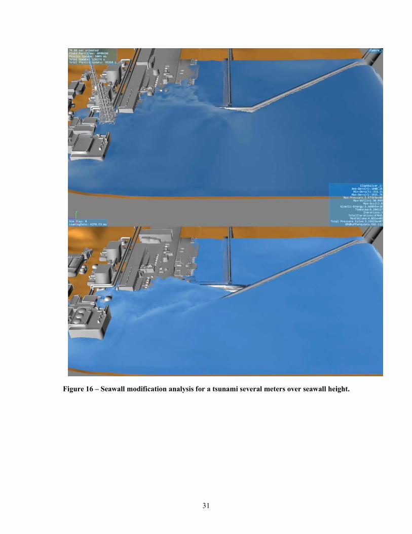
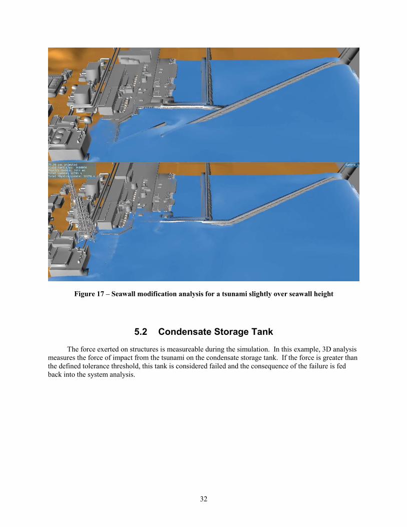
Multiple variations of the seawall configuration for a hypothetical facility were modeled and simulated at different wave heights. These simulations can be used to determine water levels and what areas are most at risk depending on the size and duration of the wave with a given configuration. This data can help with initial designs or modifications to existing facilities. In (Figure 17) we see that with the larger tsunami, there is not much difference in protection from the seawall. For a tsunami just above the same height of seawall, the modified wall is able to divert the flooding away from more critical facility areas (see Figure 17).

31

Figure 16 – Seawall modification analysis for a tsunami several meters over seawall height.

32

Figure 17 – Seawall modification analysis for a tsunami slightly over seawall height

5.2 Condensate Storage Tank

The force exerted on structures is measureable during the simulation. In this example, 3D analysis measures the force of impact from the tsunami on the condensate storage tank. If the force is greater than the defined tolerance threshold, this tank is considered failed and the consequence of the failure is fed back into the system analysis.

33

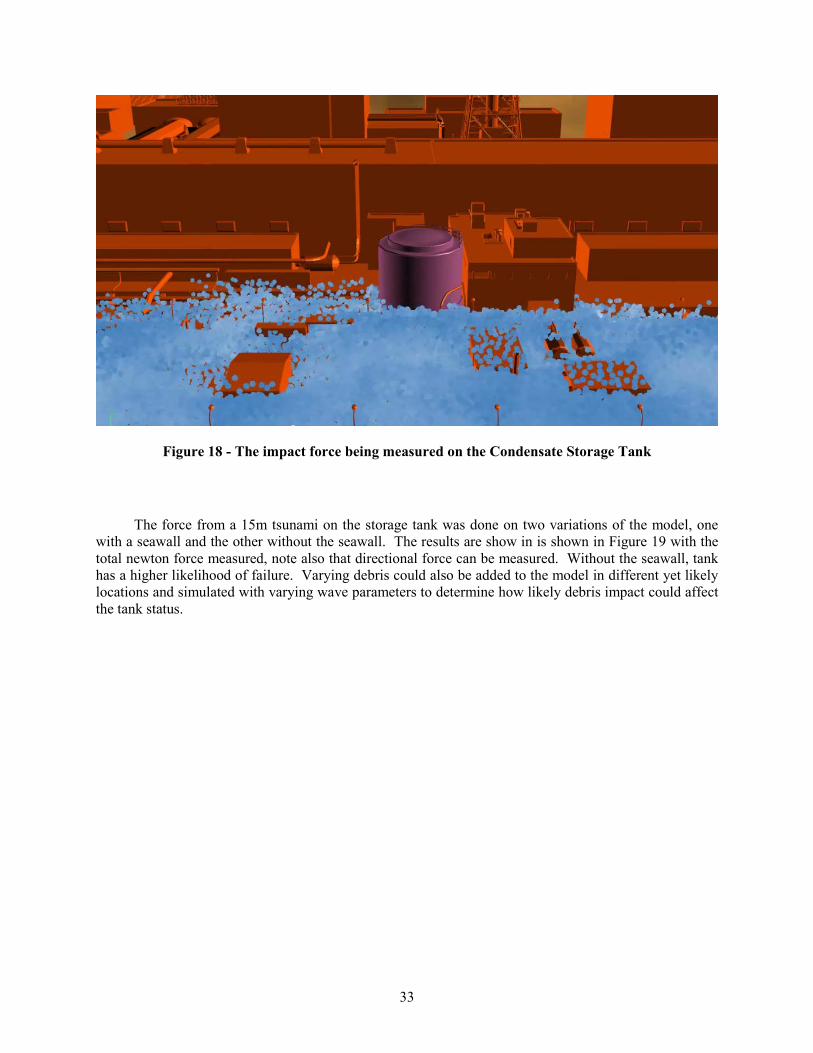
Figure 18 - The impact force being measured on the Condensate Storage Tank

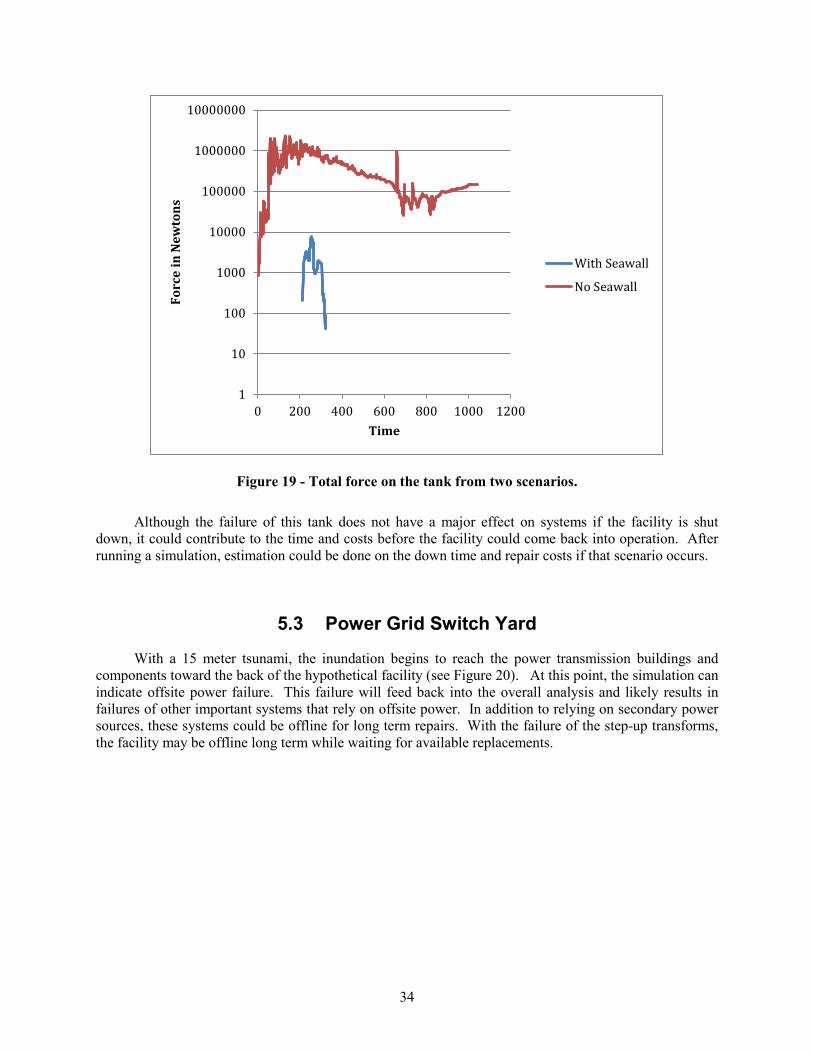
The force from a 15m tsunami on the storage tank was done on two variations of the model, one with a seawall and the other without the seawall. The results are show in is shown in Figure 19 with the total newton force measured, note also that directional force can be measured. Without the seawall, tank has a higher likelihood of failure. Varying debris could also be added to the model in different yet likely locations and simulated with varying wave parameters to determine how likely debris impact could affect the tank status.

34

Figure 19 - Total force on the tank from two scenarios.

Although the failure of this tank does not have a major effect on systems if the facility is shut down, it could contribute to the time and costs before the facility could come back into operation. After running a simulation, estimation could be done on the down time and repair costs if that scenario occurs.

5.3 Power Grid Switch Yard

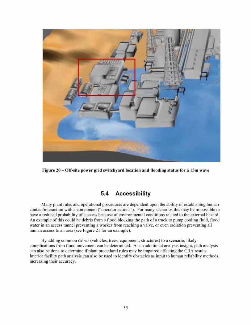
With a 15 meter tsunami, the inundation begins to reach the power transmission buildings and components toward the back of the hypothetical facility (see Figure 20). At this point, the simulation can indicate offsite power failure. This failure will feed back into the overall analysis and likely results in failures of other important systems that rely on offsite power. In addition to relying on secondary power sources, these systems could be offline for long term repairs. With the failure of the step-up transforms, the facility may be offline long term while waiting for available replacements.

1

10

100

1000

10000

100000

1000000

10000000

0 200 400 600 800 1000 1200

Forc

e in

New

tons

Time

With Seawall

No Seawall

35

Figure 20 – Off-site power grid switchyard location and flooding status for a 15m wave

5.4 Accessibility

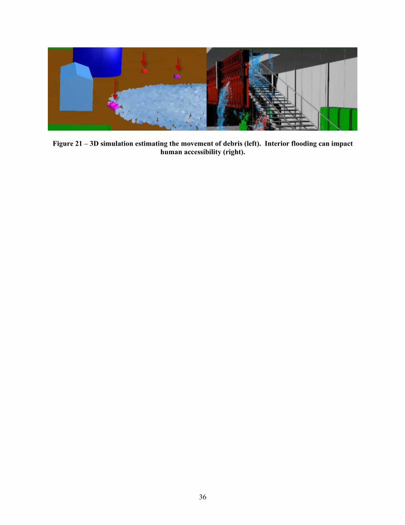
Many plant rules and operational procedures are dependent upon the ability of establishing human contact/interaction with a component (“operator actions”). For many scenarios this may be impossible or have a reduced probability of success because of environmental conditions related to the external hazard. An example of this could be debris from a flood blocking the path of a truck to pump cooling fluid, flood water in an access tunnel preventing a worker from reaching a valve, or even radiation preventing all human access to an area (see Figure 21 for an example).

By adding common debris (vehicles, trees, equipment, structures) to a scenario, likely complications from flood movement can be determined. As an additional analysis insight, path analysis can also be done to determine if plant procedural rules may be impaired affecting the CRA results. Interior facility path analysis can also be used to identify obstacles as input to human reliability methods, increasing their accuracy.

36

Figure 21 – 3D simulation estimating the movement of debris (left). Interior flooding can impact human accessibility (right).

37

6. Conclusions

Incorporating 3D simulations as part of the RISMIC Toolkit allows analysts to obtain a more complete picture of complex system behavior in a straightforward manner. External events such as flooding have become more of an issue – however these can be analyzed with existing and validated simulated physics toolkits. In this report, we describe these approaches specific to flooding-based analysis using SPH. Integrating these methods into CRA provides a spatial/visual aspect to the design, improves the realism of results, and can prove visual understanding to validate results.

38

7. References

[BYM05] N. Bell, Y. Yu, and P. J. Mucha. Particle-based simulation of granular materials. In Proc. of the 2005 ACM SIGGRAPH/Eurographics Symposium on Computer Animation, pages 77–86, 2005.

[CL03] A. Colagrossi and M. Landrini. Numerical simulation of interfacial flows by smoothed particle hydrodynamics. J. Comp. Phys., 191(2):448–475, 2003.

[Cre11] A. Crespo. User Guide for the DualSPHysics Code v1.0, 2011.

[DK01] R.A. Dalrymple and O. Knio. SPH modeling of water waves. In Proc. Coastal Dynamics, pages 779–787, 2001.

[GM77] R.A. Gingold and J.J. Monaghan. Smoothed particle hydrodynamics: theory and application to non-spherical stars. Monthly Notices of the Royal Astronomical Society, 181:375–398, 1977.

[IABT11] Markus Ihmsen, Nadir Akinci, Markus Becker, and Matthias Teschner. A parallel SPH implementation on multi-core CPUs. Computer Graphics Forum, 30(1):99–112, 2011.

[ICS+13] Markus Ihmsen, Jens Cornelis, Barbara Solenthaler, Christopher Horvath, and Matthias Teschner. Implicit incompressible sph. IEEE Transactions on Visualization and Computer Graphics, 99(PrePrints):1, 2013.

[Luc77] Leon B. Lucy. A Numerical Approach to Testing the Fission Hypothesis. The Astronomical Journal, 82(12):1013–1924, 1977.

[SM14] C. Smith, D. Mandelli, S. Prescott, A. Alfonsi, C. Rabiti, J. Cogliati, and R. Kinoshita, “Analysis of pressurized water reactor station blackout caused by external flooding using the RISMC toolkit,” Tech. Rep. INL/EXT-14-32906, Idaho National Laboratory (INL), 2014

[ML85] JJ Monaghan and JC Lattanzio. A refined particle method for astrophysical problems. Astronomy and astrophysics, 149:135–143, 1985.

[Mon05] J.J. Monaghan. Smoothed particle hydrodynamics. Reports on Progress in Physics, 68(8):1703–1759, 2005.

[NA12] Gizem Akinci Barbara Solenthaler Matthias Teschner Nadir Akinci, Markus Ihmsen. Versatile rigid-fluid coupling for incompressible sph. ACM Trans. on Graphics (SIGGRAPH Proc.), 2012.

[She68] D. Shepard. A two-dimensional interpolation function for irregularly spaced points. In Proceedings of the 23rd ACM national conference, pages 517–524, 1968.

[SRM11] C. Smith, C. Rabiti, and R. Martineau, “Risk Informed Safety Margins Characterization (RISMC) pathway technical program plan”, Idaho National Laboratory Technical Report INL/EXT-11-22977 (2011).

39

[Cum12] S. J. Cummins., etc., “Three-dimensional wave impact on a rigid structure using smoothed particle hydrodynamics”, International Journal for Numerical Methods in Fluids (2012); 68: 1471-1496, http://onlinelibrary.wiley.com/doi/10.1002/fld.2539/epdf

[CBE05] Chern, M.J., Borthwick, A.G.L. and Eatock Taylor, R. “Pseudospectral element

model for free surface viscous flows”, Int. J. Num. Meth. For Heat & Fluid Flow (2005), 15(6), 517 – 554, http://www.researchgate.net/publication/235263308_Pseudospectral_element_model_for_free_surface_viscous_flows

[Gio] I. Giosan, P.Eng, “Vortex Shedding Induced Loads on Free Standing Structures”, Structural Vortex Shedding Response Estimation Methodology and Finite Element Simulation. http://www.wceng-fea.com/vortex_shedding.pdf

[Ghi82] Ghia, U., etc., “High-Re solutions for incompressible flow using the Navier-Stokes equations and a multigrid method”, Journal of Computational Physics, v. 5, n. 48, p.387-411, 1982