Automatic Network Checkup for MobilityFeatures in 3G

Networks

André António da Costa Marques

Thesis to obtain the Master of Science Degree in

Electrical and Computer Engineering

Supervisor: Prof. António José Castelo Branco Rodrigues

Examination Committee

Chairperson: Prof. Fernando Duarte Nunes

Supervisor: Prof. António José Castelo Branco Rodrigues

Members of the Committee: Prof. António João Nunes Serrador

Eng. Pedro Luís Almeida Martins

April 2014

ii

iii

To all my family and beloved ones

iv

v

Acknowledgements

Acknowledgements

First I would like to thank professor António Rodrigues for giving me the opportunity of working with

him in the development of this work, for all the support and ideas to solve this problem.

Secondly my gratitude goes to my colleges in Alcatel-Lucent Portugal for all the support and

contributions to improve my work, mainly Artur Vargas and Pedro Martins for sharing their knowledge

and know-how about 3G technology and Alcatel-Lucent’s algorithms. For all the supervision and

availability to discuss solutions and solve blocking problems, even when time was sparse.

I also would like to thank to my colleagues from Altran Portugal for all the support and availability

shown during the development of this work.

To all my friends and colleagues who not only helped me acquire knowledge, develop skills and

overcome barriers, but also helped me to enjoy my academic life with moments of fun throughout all

this years.

To my girlfriend Ana for the patience and support during this months of lesser availability.

To my friend José Reis for the document revision.

And last, but not least, I want to thank to my parents, sister, all my family and beloved ones, for all the

support and courage given during this long path. To my grandfather António for teaching me, and

remembering me since I was little, that hard work pays off.

vi

vii

Abstract

Abstract

With the increase of mobile traffic due to new multimedia applications, video streaming and others,

mobile operators had to adapt and evolve and deploy structures and algorithms to improve the mobile

network’s capacity. To increase the network’s capacity it was developed multi-layers structures and

algorithms were developed to manage the traffic in the different layers. This work’s main objective was

to develop a tool to perform the network checkup to find different configurations implemented in the

network, and also to represent the mobility strategies implemented, in order to reduce the time spent

in the studying of the network configurations. This work is divided in three parts. First the main

concepts of the 3G/HSPA networks are presented, with special attention to the mobility procedures.

Then the mobility algorithms implemented in the network are explained. The last part presents the tool

developed to check the network configurations and as well as the implemented mobility strategies.

Keywords

UMTS, HSPA, Network Checkup Tool, Traffic Distribution, Mobility Features

viii

Resumo

Resumo

Com o aumento de tráfego móvel devido a novas aplicações multimédia, vídeo e outras, os

operadores móveis tiveram necessidade de se adaptar e desenvolver estruturas e algoritmos para

melhorar a capacidade das redes. De modo a aumentar a capacidade das redes foram desenvolvidas

estruturas multi camada e algoritmos para gerir a localização dos móveis nessas camadas. Este

trabalho teve como objectivo desenvolver uma ferramenta para verificar e representar as diferentes

configurações implementadas numa rede, assim como as estratégias de mobilidade entre as

diferentes camadas, de modo a reduzir o tempo utilizado no estudo da configuração das redes. Este

trabalho está divido em três partes. Na primeira parte são apresentados os conceitos básicos das

redes 3G/HSPA com um especial foco nos seguintes processos de mobilidade. De seguida são

explicados os algoritmos de mobilidade implementados na rede. Por ultimo é apresentada a

ferramenta desenvolvida para verificar as diferentes configurações da rede e as diferentes estratégias

de mobilidade implementadas.

Palavras-chave

UMTS,HSPA, Ferramenta para examinação da rede, Distribuição de Trafego, Estratégias de

Mobilidade

ix

Table of Contents

Table of Contents

Acknowledgements ................................................................................. v

Abstract ................................................................................................. vii

Resumo ................................................................................................ viii

Table of Contents ................................................................................... ix

List of Figures ........................................................................................ xi

List of Tables ......................................................................................... xiii

List of Acronyms .................................................................................. xiv

List of Symbols ..................................................................................... xvii

List of Software ................................................................................... xviii

1 Introduction .................................................................................. 1

1.1 Overview.................................................................................................. 3

1.2 Motivation and Contents .......................................................................... 3

2 Basic Concepts ............................................................................ 7

2.1 Radio Interface - Spectrum and Medium Access ..................................... 9

2.2 UMTS System ....................................................................................... 12

2.2.1 System Architecture ............................................................................................ 12

2.2.2 Network Protocols................................................................................................ 13

2.2.3 Channels .............................................................................................................. 14

2.3 RRC Protocol ......................................................................................... 16

2.3.1 RCC States .......................................................................................................... 16

2.3.2 System Information Block .................................................................................... 17

2.3.3 RRC Connection Establishment and RRC Connection Release ........................ 18

2.4 Call Admission Control .......................................................................... 19

2.5 Cell Selection/Reselection and Mobility ................................................. 20

2.5.1 Cell Selection and Cell Reselection..................................................................... 20

2.5.2 Handover Procedures .......................................................................................... 22

x

2.6 HSPA/HSPA+ ........................................................................................ 24

2.6.1 HSPA ................................................................................................................... 24

2.6.2 HSPA+ ................................................................................................................. 24

2.6.3 UE Categories ..................................................................................................... 25

3 Network Characterization and Traffic Distribution Algorithms ..... 27

3.1 RNC Snapshot ....................................................................................... 29

3.2 Cell Concept Configuration .................................................................... 30

3.3 Cell Reselection Strategy ...................................................................... 31

3.4 RRC Redirection .................................................................................... 32

3.5 Traffic distribution in cell DCH ............................................................... 35

3.6 Network Summary ................................................................................. 37

4 Network Checkup Tool ............................................................... 39

4.1 Parameters database and snapshot structure ....................................... 41

4.2 Algorithm Description ............................................................................ 43

4.3 User Interface and tool output ............................................................... 47

4.4 Performance and Output evaluation ...................................................... 51

5 Conclusions and Future Works................................................... 55

5.1 Conclusions ........................................................................................... 57

5.2 Future Works ......................................................................................... 58

Annex A. Parameters Type and XML Structures ....................................................................... 59

A.1 Parameters Fields .......................................................................................................... 61

A.2 Parameter type configuration and XML file structure ..................................................... 61

References............................................................................................ 67

xi

List of Figures

List of Figures Figure 1.1 Multi-Layer Configuration [4]. .................................................................................................. 4

Figure 2.1 Spreading and scrambling process [2]. .................................................................................11

Figure 2.2 UMTS System Architecture [6]. ............................................................................................12

Figure 2.3 Channel Representation. ......................................................................................................14

Figure 2.4 UE Modes and Connected Mode States (adapted from [2]). ................................................16

Figure 2.5 RRC Connection Establishment message flow. ...................................................................18

Figure 2.6 Call Admission Control Procedure and CAC failure. .............................................................19

Figure 2.7 Cell Ranking Algorithm. .........................................................................................................21

Figure 2.8 Soft Handover Scheme. ........................................................................................................22

Figure 2.9 Example of Event 2D and 2F. ...............................................................................................23

Figure 3.1 9359 WPS Graphical Interface. .............................................................................................30

Figure 3.2 RRC Redirection Strategy [4]. ...............................................................................................34

Figure 3.3 Example of a priority table [4]. ...............................................................................................36

Figure 3.4 Example of the network summary. ........................................................................................37

Figure 4.1 Example of the XML structure of a generic parameter. ........................................................42

Figure 4.2 General representation of the snapshot XML structure. .......................................................43

Figure 4.3 Network Information Import. ..................................................................................................44

Figure 4.4 Node B configuration check. .................................................................................................45

Figure 4.5 Network Representation and parameter report creation. ......................................................46

Figure 4.6 Windows interface for snapshot location. .............................................................................47

Figure 4.7 Progress bar. .........................................................................................................................48

Figure 4.8 Finish window. .......................................................................................................................48

Figure 4.9 Example of one graphical representation of the reselection strategy. ..................................48

Figure 4.10 – Example of graphical representation of RRC redirection strategy. ..................................49

Figure 4.11 Structure of the parameters report. .....................................................................................50

Figure 4.12 Network A's Summary extracted from the Excel report. .....................................................51

Figure 4.13 Network B's summary extracted from the Excel report. ......................................................51

Figure 4.14 Network C's summary extracted from the excel report. ......................................................51

Figure 4.15 Cell Reselection strategy representation. ...........................................................................52

Figure 4.16 RRC redirection strategy (IMCRA Step 2 Service) representation. ....................................53

Figure 4.17 Traffic distribution in cell DCH (IMCTA Alarm) strategy representation..............................53

Figure 4.18 Traffic distribution in cell DCH (IMCTA CAC) strategy representation. ..............................54

Figure A.1 Fields used in the parameter characterization. .....................................................................61

Figure A.2 Configuration of the field Value for one parameter type Number .........................................62

Figure A.3 XML structure of a parameter type Number. ........................................................................62

Figure A.4 XML structure of a parameter type number. .........................................................................62

Figure A.5 Content of the feild Values for one parameter type Enum. ..................................................63

Figure A.6 XML structure of a parameter type Enum. ............................................................................63

Figure A.7 Configuration of the Value field for the parameter type IntList. ............................................63

xii

Figure A.8 XML structure of a parameter type number. .........................................................................64

Figure A.9 XML structure of a parameter type number. .........................................................................64

Figure A.10 Configuration of the parameter type Binary. .......................................................................65

Figure A.11 XML structure of a parameter type number. .......................................................................65

xiii

List of Tables

List of Tables Table 2.1 ARFCN specific values for channel number calculation (adapted from [5])...........................10

Table 2.2 System Information Block Description. ..................................................................................17

Table 2.3 HSDPA UE Categories (adapted from [13]). ..........................................................................25

Table 3.1 Layer concept definition. ........................................................................................................31

Table 4.1 Parameter type description for the excel macro input. ...........................................................41

Table 4.2 Network Characterizations .....................................................................................................51

xiv

List of Acronyms

List of Acronyms 2G 2

nd Generation

3G 3rd

Generation

3GPP 3rd

Generation Partnership Project

ALU Alcatel-Lucent

BCCH Broadcast Control Channel

BCH Broadcast Channel

BS Base Station

CAC Call Admission Control

CCH Control Channel

CM Compressed Mode

CN Core Network

CPICH Common Pilot Channel

CS Circuit Switched

CS-CN Circuit Switched Core Network

DC Dual Cell

DCH Dedicated Channel

DC-HSDPA Dual-Cell HSDPA

DL Downlink

DS-CDMA Direct-Sequence Code Division Multiple Access

E-DCH Enhanced-DCH

ETSI European Telecommunication Standard Institute

FACH Forward Access Channel

FDD Frequency Division Duplexing

GSM Global System for Mobile Communications

HHO Hard Handover

HO Handover

HSDPA High-Speed Downlink Packet Access

HS-DSCH High-Speed Downlink Shared Channel

HSPA/HSxPA High-Speed Packet Access

HSUPA High-Speed Uplink Packet Access

IMCRA Intelligent Multi-Carrier RRC Redirection Traffic Allocation

IMCTA Intelligent Multi-Carrier Traffic Allocation

MAC Medium Access Control

MIB Master Information Block

xv

MIMO Multiple Input Multiple Output

MS Mobile Station

MSA Mobile Station A

MSB Mobile Station B

NBAP Node B Application Protocol

OVSF Orthogonal Variable Spreading Factor

P-CCPCH Primary Common Control Physical Channel

PCH Paging Channel

PLMN Public Land Mobile Network

PNA Priority Not Assigned

PS Packet Switched

PS-CN Packet Switched Core Network

QoS Quality of Service

R5 Release 5

R6 Release 6

R99 Release 99

RAB Radio Access Bearer

RANAP Radio Access Network Application Protocol

RAT Radio Access Technologies

RB Radio Bearer

RLC Radio Link Control

RNS Radio Network Subsystem

RNSAP Radio Network Sub-system Application Protocol

RRC Radio Resource Control

RSCP Received Signal Code Power

RSSI Received Signal Strength Indicator

S-CCPCH Secondary Common Control Physical Channel

SF Spreading Factor

SHO Soft Handover

SIB System Information Block

SIR Signal-to-Interference Ratio

SRB Signalling Radio Bearer

TCH Traffic Channel

TDD Time Division Duplex

TTI Transmission Time to Interval

UA UTRAN Architecture

UARFCN UTRAN Absolute Radio Frequency Channel Number

UE User Equipment

UL Uplink

UMTS Universal Mobile Telecommunication System

xvi

URA UTRAN Registration Area

UTRAN UMTS Terrestrial Radio Access Network

WCDMA Wideband Code Division Multiple Access

XML eXtended Markup Language

xvii

List of Symbols

List of Symbols

Ec/No Relation between the RSCP and the RSSI

Downlink carrier frequency

Downlink upper bound of the operating band

Downlink lower bound of the operating band

Uplink carrier frequency

Uplink upper bounds of operating band

Uplink lower bounds of operating band

Downlink UARFCN value

Uplink UARFCN value

Compensation factor used to penalize the low power UE

Quality of the received signal measured by the UE

Minimum quality required

Received signal power measured by the UE

Minimum received power level

xviii

List of

List of Software Microsoft Excel Microsoft application to treat large amount of data

VBA Microsoft application that allows developing applications to process data over Microsoft Excel

Alcatel-Lucent 9352 WPS

The 9352 WPS allows users to configure, change and optimize parameters of the WCDMA access network

Java SE Programing tool to develop java platforms applications

1

Chapter 1

Introduction

1 Introduction

This chapter gives a brief overview of the work. Firstly motivation for the thesis is presented. Secondly

the document structure is provided.

2

3

1.1 Overview

Universal Mobile Telecommunication System (UMTS) was developed to complement the 2nd

Generation (2G), also known as Global System for Mobile Communications (GSM). It offered a new

cluster of multimedia services that were not supported by the 2G systems. An example for the

multimedia services is the video-telephony and the internet access [1].

Wideband Code Division Multiple Access (WCDMA) was adopted as the air interface for the 3rd

Generation (3G) mobile communication system early in 1998 by the European Telecommunication

Standard Institute (ETSI). The first group of specification was released one year later, in 1999 by the

3rd

Generation Partnership Project (3GPP) and for this reason called Release 99 (R99). The first

commercial network was developed in Japan in the year of 2001. One year later, in the beginning of

2002 the first network was developed in Europe [2].

With R99 bit rates up to 2 Mbps were expected, but after all only 384 kbps were achieved. Due to this

reason and also for the growth of data communications, new releases were developed by 3GPP in

order to obtain higher capacity, throughput and better Quality of Service (QoS). In March of 2002, the

specifications of the Release 5 (R5) were published to improve, among others, the downlink (DL)

throughput. High-Speed Downlink Packet Access (HSDPA) was one of the main features of R5. It has

introduced, in between other features, a new downlink channel. The maximum rate for HSDPA is 14.4

Mbps.

In the end of 2004, Release 6 (R6) specifications to improve the Uplink (UL) services were

standardized. It introduced the High-Speed Uplink Packet Access (HSUPA) and a maximum UL peak

rate of 5.4 Mbps. The enhancements introduced with release 5 and 6 became kwon as High Speed

Packet Access (HSPA/HSxPA).

HSPA evolution is known as HSPA+, was specified in the Release 7 in 2006. It introduces the Multiple

Input Multiple Output and Release 8 adds the Dual Cell (DC) HSDPA features. In parallel with the

network evolution, new mobile devices also were deployed to take advantage of the new network

capacities.

In the beginning of October 2013 there were more than 500 HSPA networks in service over 200

different countries and around 300 HSPA+ networks over 132 countries [3].

1.2 Motivation and Contents

To increase network capacity, operators may develop multi-layers configurations with different layers.

Analogue to this multi-layer configuration it was necessary to develop features which allowed

distributing traffic efficiently through different layers, including other Radio Access Technologies (RAT)

[4].

4

Figure 1.1 Multi-Layer Configuration [4].

Two different multi-layer topologies can be deployed:

Symmetric topologies where HSxPA/Data traffic and non HSxPA/Conversational traffic cohabit

in the same layer. [4].

Asymmetric topologies, as presented in Figure 1.1, where there is a dedicated layer for

HSxPA/Data traffic (FDD2) and other layer for non HSxPA/Conversational traffic (FDD1). [4].

To ensure that mobile devices select the right layer to perform the calls, Alcatel-Lucent (ALU)

developed traffic distribution algorithms that are in charge to distribute the mobile devices along the

correct layers. The traffic distribution can be performed based in the layer overload or in the layer

topology. Usually the first case is used in symmetric topologies while the second one is used in

asymmetric topologies.

These traffic distribution algorithms can be implemented during 3 different stages, cell reselection,

Radio Resource Control (RRC) connection establishment and also during Handover (HO) procedure.

The procedures enumerated previously are better explained in Chapter 2.

The algorithms are configured in the network with parameters. With the increase of traffic in the

mobile networks, the dimension of the networks also increased and these algorithms have become

more complex to answer the network needs. This complexity growth leads to a huge increase of new

parameters and new possible configurations. Due to these algorithm’s complexity, checking which

mobility strategy is applied in each layer can be a complex and time consuming task.

5

For the reasons presented in the previous paragraph, the current thesis is motivated by the necessity

of automatically check which are the configurations developed in a network, which mobility strategies

are applied and also to represent these mobility strategies in a way of easy interpretation. It is also

with this automatic checkup intended to reduce the duration of the configuration checkup task that

depending on the network size can be a time consuming task.

To improve the network checkup procedure a tool was developed that summarises the network

configuration and generates two different reports. This tool processes the Radio Network Control

(RNC) parameterization from ALU UMTS Terrestrial Radio Access Network (UTRAN) Architecture

(UA) 8.1. As output it retrieves the different network configurations as well as the configuration of the

traffic distribution algorithm implemented in the processes as referred previously.

This thesis is divided in five chapters. In the first chapter the motivations for the development of this

work are presented, as well as the work’s structure. In the second chapter the basic concepts of the

3G network are presented, with a special attention to the mobility procedures under study.

The third chapter is divided in two main parts. In the first part the network parameterization, different

parameters type and characteristics and the parameter organization in the network are presented. In

the second part the different traffic distribution algorithms and the main features of each one are

explained. Finally the main difficulties and limitations in the network checkup process are presented.

In chapter four, the tool’s main features are presented. First a brief overview of the parameters

database built to the tool is given. Then the algorithm developed for the network checkup process is

described. At last the tool performance and the output generated are evaluated using different

networks as examples.

In the fifth and last chapter, the main conclusions and suggestions for future work are stated, as new

features that can be integrated in the toll or application in other RAT. In the end of the document there

are three annexes for a better comprehension of the ALU algorithms, the description of the main

parameter used in each mobility features and the structure of the parameters database.

6

7

Chapter 2

Basic Concepts

2 Basic Concepts

This chapter provides an overview of the UMTS, HSDPA and HSUPA systems, with special detail to

the mobility procedures.

8

9

2.1 Radio Interface - Spectrum and Medium Access

UMTS uses Wideband Code Division Multiple Access as the multiple access technique in the radio

interface. WCDMA is a wideband Direct-Sequence Code Division Multiple Access (DS-CDMA)

system.

WCDMA has two possible working modes, Frequency Division Duplex (FDD) and Time Division

Duplex (TDD). For the scope of this thesis only WCDMA FDD will be considered.

Defined by 3GPP, the carrier frequency is designated by UTRA Absolute Radio Frequency Channel

Number (UARFCN) [5]. The channel spacing is 5MHz and the separation between two adjacent

channels is 200 kHz. The formulas to compute the Uplink (UL) and Downlink (DL) UARFCN are

presented in equation 2.1 and 2.2 respectively.

( ) (2.1) [5]

( ) (2.2) [5]

Where:

is the carrier frequency in MHz

and are the lower and upper bounds of operating band in MHz, in the uplink

is the downlink carrier frequency in MHz

and are the lower and upper bounds of operating band in MHz, in the

downlink

In Table 2.1, for each operating band, the , , , , values are presented. The

lower and higher channels are also presented.

Additional channels were added in some bands. The UARFCN specific offsets and carrier frequency

for these additional channels can be consulted in [5].

Regarding DS-CDMA, it uses a spread spectrum modulation. The spread spectrum modulation is a

technique that spreads the information to be transmitted over the available bandwidth. At the

transmitter the signal is multiplied by a code that spreads the signal all over the bandwidth. As the

receiver knows which was the spreading code used by the transmitter, it is able to recover the signal.

10

Table 2.1 ARFCN specific values for channel number calculation (adapted from [5]).

Band [MHz]

UPLINK

Band [MHz]

Downlink

Carrier Frequency ( ) range [MHz]

Carrier Frequency ( ) range [MHz]

1920-1980 0 1992.4 1977.6 2110-2170 0 2112.4 2167.6

1850-1910 0 1852.4 1907.6 1930-1990 0 1932.4 1987.6

1710-1785 1525 1712.4 1782.6 1805-1880 1575 1807.4 1877.6

1710-1755 1450 1712.4 1752.6 2110-2155 1805 2112.4 2152.6

824-849 0 826.4 846.6 869-894 0 871.4 891.6

830-840 0 832.4 837.6 875-885 0 877.4 882.6

2500-2570 2100 2502.4 2567.6 2620-2690 2175 262.4 2687.6

880-915 340 882.4 912.6 925-960 340 927.4 957.6

1749.9-1784.9 0 1752.4 1782.4

1844.9-1879.9 0 1847.4 1877.4

1710-1770 1135 1712.4 1767.6 2110-2170 1490 2112.4 2167.6

1427.9-1447.9 733 1430.4 1445.4

1475.9-1495.9 736 1478.4 1493.4

699-716 -22 701.4 713.6 729-746 -37 731.4 743.6

777-787 21 779.4 784.6 746-756 -55 748.4 753.6

788-798 12 790.4 795.6 758-768 -63 460.4 765.6

830-845 770 832.4 842.6 875-890 735 877.4 887.6

832-862 -23 834.4 859.6 791-821 -109 793.4 818.6

1447.9-1462.9 1358 1450.4 1460.4

1495.9-1510.9 1329 1498.4 1508.4

3410-3490 2525 3412.4 3487.6 3510-3590 2580 3512.4 3587.6

1850-1915 875 1852.4 1912.6 1930-1995 910 1932.4 1992.6

814-849 -291 816.4 846.6 859-894 -291 861.4 891.6

The spreading sequence is characterized by the Spreading Factor (SF). It indicates the length of the

code used in the spreading operation. The spread spectrum modulation uses the Orthogonal Variable

Spreading Factor (OVSF) technique to guarantee that even when the SF is changed, the codes keep

the orthogonally between them. [2]

The SF is the number of chips multiplied for each bit. In the uplink the spreading factors available are

4, 8, 16, 32, 64, 128, and 256, while in the downlink the spreading factor varies between 4 and 512.

The spreading factor is also known as the number of chips per bit. The chip rate has a constant value

of 3.84 Mcps. [6]

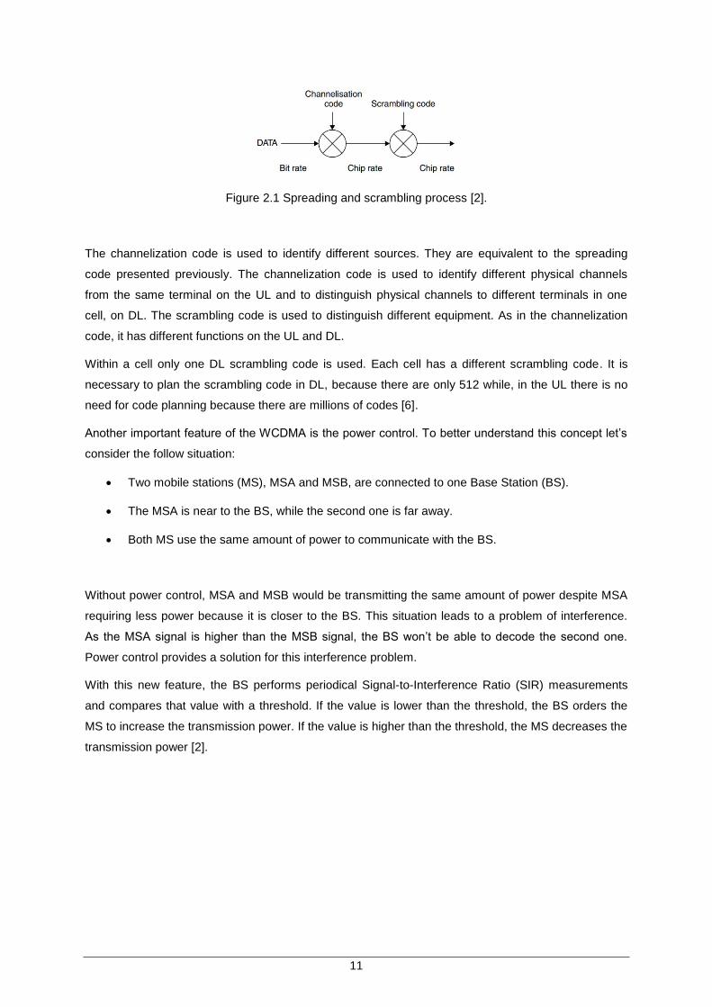
In WCDMA all users transmit on the same carrier and at the same time. To distinguish the several

users or base stations a scrambling operation was introduced. The scrambling operation comes after

the spreading operation as presented in Figure 2.1.

11

Figure 2.1 Spreading and scrambling process [2].

The channelization code is used to identify different sources. They are equivalent to the spreading

code presented previously. The channelization code is used to identify different physical channels

from the same terminal on the UL and to distinguish physical channels to different terminals in one

cell, on DL. The scrambling code is used to distinguish different equipment. As in the channelization

code, it has different functions on the UL and DL.

Within a cell only one DL scrambling code is used. Each cell has a different scrambling code. It is

necessary to plan the scrambling code in DL, because there are only 512 while, in the UL there is no

need for code planning because there are millions of codes [6].

Another important feature of the WCDMA is the power control. To better understand this concept let’s

consider the follow situation:

Two mobile stations (MS), MSA and MSB, are connected to one Base Station (BS).

The MSA is near to the BS, while the second one is far away.

Both MS use the same amount of power to communicate with the BS.

Without power control, MSA and MSB would be transmitting the same amount of power despite MSA

requiring less power because it is closer to the BS. This situation leads to a problem of interference.

As the MSA signal is higher than the MSB signal, the BS won’t be able to decode the second one.

Power control provides a solution for this interference problem.

With this new feature, the BS performs periodical Signal-to-Interference Ratio (SIR) measurements

and compares that value with a threshold. If the value is lower than the threshold, the BS orders the

MS to increase the transmission power. If the value is higher than the threshold, the MS decreases the

transmission power [2].

12

2.2 UMTS System

2.2.1 System Architecture

In a high level view the UMTS system architecture can be divided in two main domains, the User

Equipment (UE) domain and the infrastructure domain [7]. The infrastructure domain comprises the

UTRAN and the Core Network (CN). In Figure 2.2 is presented the UMTS System Architecture.

Figure 2.2 UMTS System Architecture [6].

The UE is the mobile terminal which allows the user access to network services. The interface

between the UE and the UTRAN, Uu, is defined by 3GPP as “Radio Interface between UTRAN and

the User Equipment” [8].

The UTRAN is composed by two distinct elements.

Node B: is responsible for the radio communication in one or more cells with the UE. It

converts the data from Uu to Iub interface. A cell is the radio network element broadcasted by

the node B and uniquely identified by the UE [8].

Radio Network Controller: Element in charge of controlling and managing the radio

resources. It is also the access point of UTRA services to the CN [8].

As the CN is out of scope for this thesis, it will only be presented two sub groups, the Circuit Switched

(CS) CN and the Packet Switched (PS) CN. The first one provides CS connections while the second

one is responsible for the PS connections, both to external networks.

13

Although the network elements have been specified by 3GPP, their implementation was left

unspecified aiming at competition between different manufacturers. Nevertheless, to allow

interoperability between elements from different manufacturers, the interfaces between the network’s

elements have been standardised [6].

The interfaces are:

Uu interface: As referred previously the Uu interface connects the UE to the UTRAN.

Iub interface: Interface that connects the Node B and the RNC.

Iur interface: This interface supports the communication between RNCs and allows soft

handover between cells of RNCs from different manufacturers.

Iu interface: The Iu interface can be Iu-CS and Iu-PS depending on whether it is connected to

the PS-CN or CS-CN. It provides a point of interconnection between the RNC and CN.

2.2.2 Network Protocols

Running over the different interfaces are the network protocols. They can be grouped by Iu protocols

which run over the Iu interfaces, and by radio protocols who run over the Uu interface.

The Iu protocols are the following:

Radio Access Network Application Protocol (RANAP): it is responsible for the signalling

between the UTRAN and the CN. It is responsible, among others, by relocation of serving

RNC, manage all Radio Access Bearer (RAB) procedures and also Iu resources release [2].

Radio Network Sub-system Application Protocol (RNSAP): is used to carry signalling over the

Iur. It is responsible to the communication between two RNCs.

Node B Application Protocol (NBAP): it is responsible to carry signalling between Node B and

RNC over the Iub interface. It is responsible, among others, for reserving radio resources for

the radio link [2].

The radio protocols are the following:

Radio Resource Control (RRC): This protocol is responsible by the RRC connections and the

Radio Bearer connections management. It is also responsible by the radio channel ciphering

and deciphering, and responsible for radio mobility management.

Radio Link Control (RLC): It is responsible for Radio Link connection management. It is

responsible for the control of the radio bearer service.

Medium Access Control (MAC): it is responsible, among others, by multiplex logical channels,

map logical channels to transport channels.

Later in this document, it will be given special attention to the RRC protocol.

14

2.2.3 Channels

There are three types of channels in the UMTS technology: logical channels, transport channels and

physical channels. On top of these three channels stands the Radio Bearers (RB). They are controlled

by the RAB service. This service is responsible for the transport of data and signalling between UE

and the CN, with reliability and with the required QoS. It can be split between Radio Bearers (RB) and

Iu bearers. The protocol responsible for the RAB management is the RANAP.

There are two types of RB. Signalling Radio Bearers (SRB) and user plane RBs. The first one, as its

name implies, is responsible to carry all the signalling. The second one is responsible to carry user

data. [6]

In the Figure 2.3 a high level view of the channels hierarchy is presented. On top of the hierarchy

stand the logical channels mapped successively on transport channels and physical channels.

Physical Channel

Transport Channel

Logical Channel

UE UTRAN

Figure 2.3 Channel Representation.

The logical channels can be divided into two groups: Control Channels (CCH) and Traffic Channels

(TCH). The first one is used to transfer system information, while traffic channels are used to transfer

user information [3].

The transport channels are responsible to carry higher layers data from UTRAN to the UE. The

information is transported in transport blocks that can be organized in different transport block sets.

This block structure allows to allocate different bit rates for different services. In this way the data is

organized and sent to the UE according the QoS required.

The transport channels are divided in two groups: common channels that are shared by all the UE in

the cell and Dedicated Channels (DCH) that are allocated for one UE only.

In the lower level of the channels' hierarchy there are the physical channels. Physical channels are

used to map transport channels. They are defined by a specific frequency and scrambling code.

15

Some of the physical channels are associated with transport channels and some are not. The physical

channels associated with transport channels can be dedicated to a single UE or common to a group of

UEs. They are used to carry UTRAN and CN signalling. They are also used to carry user data.

For the interest of this work, it will be given special attention to the Broadcast Control Channel

(BCCH). The BCCH is a downlink channel that is used to transport system control information.

The BCCH can be mapped over two different common transport channels: Broadcast Channel (BCH)

and the Forward Access Channel (FACH).

BCH is a downlink transport channel that transmits UTRA specific information. It is transmitted

with a low bit rate to ensure that all UEs can decode the information and with high power to

reach all users in the cell.

The FACH is also a downlink transport channel that can be used to transport control

information to UEs or small amount of data.

Although the BCCH is mapped in to different transport channels, they also are mapped in to two

different physical channels. BCH is mapped over the Primary Common Control Physical Channel (P-

CCPCH) while FACH is mapped over the Secondary Common Control Physical Channel (S-CCPCH).

The group of physical channels that are not associated with transport channels are used to carry

physical signalling. For the scope of these it will be given special attention to the group of physical

channels, with focus on the Common Pilot Channel (CPICH).

The Common Pilot Channel is a DL channel with a fixed rate of 30 kbps. It is used in the handover’s

procedure and in the cell selection/reselection. It is also used as phase reference for other channels.

There are two types of CPICH, the Primary CPICH and the Secondary CPICH.

As mentioned in the previous paragraphs, CPICH measurements are used in the handover and/or cell

selection/reselection procedures.

The UE is capable of measure three quantities over the CPICH: Received Signal Code Power

(RSCP), Received Signals Strength Indicator (RSSI) and Ec/No [9].

The RSCP is the received power on one code measured on the P-CPICH [9].

The RSSI is the received wideband power including thermal noise and noise generated in the

receiver, within the channel bandwidth [9].

The Ec/No is the relation between the RSCP and the RSSI represented on the equation (2.3)

(2.3)

16

2.3 RRC Protocol

The RRC protocol is responsible for several tasks, among them, the establishment, maintenance and

release of RRC connections between UE and UTRAN, resource management, broadcasts of system

information, cell selection and reselection procedures, RRC connection mobility functions and UE

measurement reporting and control [10].

2.3.1 RCC States

There are two main RRC modes for the UE to be. They are the idle mode and connected mode.

Connected mode, as shown in Figure 2.4 is divided in 4 states, Cell DCH, Cell FACH, URA PCH and

Cell PCH.

Idle Mode

Cell DCH

Cell FACH

URA PCH

Cell PCH

Connected Mode

Figure 2.4 UE Modes and Connected Mode States (adapted from [2]).

After the UE is turned on it will select one Public Land Mobile Network (PLMN) and a suitable cell to

camp on. When the UE finds a suitable cell, the UE enters in idle mode. In this mode the UE is

capable of, among other things, receiving system information and perform cell reselection

measurements to search for a better cell to camp on. The cell selection and cell reselection

procedures are described in section 2.5.1. In connected mode the UE is capable to transmit data to

the network.

The main difference between each state, in connected mode, is the used channel. When the UE is in

Cell DCH state it has one DCH assigned. It performs measurements, and reports the measured

values to the RNC. In cell FACH state the UE doesn’t have one dedicated channel, it uses the FACH

and RACH channels to receive and transmit data.

In Cell PCH and URA PCH the UEs are in a low battery consumption state. In cell PCH, cell FACH

and URA PCH the UE is capable of receiving system information and perform cell reselection, while in

cell DCH the UE has to perform handover to change cell.

17

The UE switches from idle mode to connected mode when a RRC connection request is accepted. If

the RRC connection is released or the connection fails, the UE returns to idle mode until new

connection is requested.

2.3.2 System Information Block

The system information may come from different sources, such as the CN, the RNC or the Node B. It

can contain static information, like the cell identity, and also dynamic information like the UL

interference level [10].

The system information is sent to the UE over the BCCH that in is turn can be mapped in the BCH or

FACH transport channel.

The system information elements are grouped together considering their characteristics. A group of

system information elements with the same characteristics form a System Information Block (SIB).

Different SIBs can also have different characteristics, like their frequency. At the top of the hierarchical

structure of the system information stands the Master Information Block (MIB).

The MIB is responsible for giving the reference and scheduling information to the SIBs in a cell [10]. It

is possible that the MIB contains one or two Scheduling Blocks. Scheduling blocks, when present, are

responsible for providing scheduling and reference information for a specific number of SIBs.

In Table 2.3 is presented some relevant SIBs for the comprehension of this thesis. SIB3 and SIB4

contain the same kind of information, cell selection and sell reselection data. If SIB4 is broadcasted,

then the UE will use these information when it is in cell FACH, cell PCH and URA PCH states. In this

case SIB3 will only be used when UE is in idle mode. If SIB4 is not broadcasted, then SIB3 will be

used in idle mode and in cell FACH, cell PCH and URA PCH states [4].

For SIB11 and SIB 12 the procedure is similar, the UE will use SIB11 when it is in idle mode and in

cell FACH, cell PCH and URA PCH states. If SIB12 is broadcasted, the UE will use it when in cell

FACH, cell PCH and URA PCH states [4].

Table 2.2 System Information Block Description.

System Information Block

Description UE mode/ state when the SIB is read

SIB3 Contains cell selection and

reselection parameters for the serving cell

Idle mode

Cell FACH, Cell PCH, URA PCH (if SIB4 is not present)

SIB4 Contains cell selection and

reselection parameters for the serving cell

Cell FACH, Cell PCH, URA PCH

SIB11 Contains cell information list dedicated to cell reselection when the UE is in idle mode

Idle mode

Cell FACH, Cell PCH, URA PCH (if SIB12 is not present)

SIB12 Contains cell information list dedicated to cell reselection

Cell FACH,Cell PCH, URA PCH

18

2.3.3 RRC Connection Establishment and RRC Connection Release

The UE only switches from idle mode to connected mode and backwards if a RRC Connection

Establishment or a RRC Connection Release is performed, respectively. To be able to transmit

signalling and data, the UE must to be in connected mode. If the UE is in idle mode it must perform a

RRC connection establishment procedure to switch from idle to connected mode [6].

RRC Connection Establishment

The RRC Connection establishment procedure is always initiated by the UE but it can be triggered by

the UE or the CN. When triggered by the CN it is preceded by a paging message. As can be seen in

Figure 2.5, the RRC Connection Establishment procedure is composed by 3 messages between the

UE and the UTRAN, the RRC Connection request, the RRC Connection set-up and finally the RRC

Connection set-up complete.

RRC Connection Request

RRC Connection set-up

RRC Connection set-up complete

UE UTRAN

Connected Mode

Idle Mode

Figure 2.5 RRC Connection Establishment message flow.

In the first message, RRC Connection Request, the UE sends to the UTRAN its identity, the

establishment cause, and the UE capability. The RRC Connection SETUP message contains the

channel information allocated to the UE. After the reception of the RRC Connection SETUP, the UE

replies with the RRC Connection setup complete. At that time the UE enters in connected mode

(Cell_DCH).

RRC Connection Release

When the UTRAN initiates the RRC Connection release procedure the UE is either in Cell FACH or

Cell DCH. The UTRAN can at any moment send a RRC Connection Release message to the UE, with

the connection release cause. The UE replies with the RRC connection release complete and it goes

back to idle mode. If the UE is in CELL FACH state it won’t reply to the UTRAN, it just leaves the

connected mode.

19

2.4 Call Admission Control

The Call Admission Control (CAC) is the procedure responsible to establish all the connections to start

a call [11]. It can be split in 3 main steps:

1. RRC Connection Establishment

2. Radio Access Bearer Assignment

3. Radio Bearer Setup

The first stage of CAC is the RRC connection establishment. In this step a Signalling Radio Bearer is

established to transmit all the signalling between the UE and the UTRAN.

\

UE UTRAN CN

RRC Connection Establishment

RAB AssignmentRadio Bearer Setup

CAC Failure

CAC Failure

Figure 2.6 Call Admission Control Procedure and CAC failure.

After the RRC connection establishment, the RAB assignment procedure is started. It is responsible to

allocate the resources, in order to guarantee the QoS required. The CN sends a RAB assignment

request to the UTRAN. In case all the resources are available, a RB is established between UE and

UTRAN. At this point the RAB assignment is completed and the CAC procedure is finished. The UE is

then able to send information [6].

CAC Failure:

If the UTRAN doesn’t have enough resources available, the CAC is not finished and the CAC failure is

triggered. These failures can happen during the RRC connection establishment and during the RAB

establishment, as highlighted in the Figure 2.6.

The UTRAN checks if it has enough resources (codes and power) when establishing RRC connection

and during the RAB assignment. If the resources are not available, the CAC procedure fails [12].

20

2.5 Cell Selection/Reselection and Mobility

2.5.1 Cell Selection and Cell Reselection

Cell Selection

When a UE is turned on it will select a Public Land Mobile Network (PLMN) and will start searching for

a suitable cell to camp on. A suitable cell is the one that belongs to one selected PLMN or equivalent.

It is not barred, does not belong to a forbidden area and satisfies the cell selection criterion S. If a

suitable cell is found the UE will camp on it and enter idle mode.

The cell selection criteria S is a selection method that uses the quality signal level and the power

signal level to check if a cell is good to be selected. The cell selection criteria S are fulfilled when the

cell selection quality value (Squal) and the cell selection Rx level value (Srxlev) are higher than zero

(Squal>0 and Srxlev>0).The equations (2.4) and (2.5) show how the values are computed [4].

(2.4)

(2.5)

is the quality of the received signal measured by the UE, CPICH EC/N0.

is the received signal power measured by the UE, CPICH RSCP.

is the minimum quality required.

is the minimum received power level.

is a compensation factor used to penalize the low power UE.

If the criteria are fulfilled the UE can camp on that cell and move to the camped normally state. In that

state the UE monitors relevant system information blocks, performs measurements and executes cell

reselection procedures [4].

Cell Reselection:

In both states the UE will perform cell reselection evaluation procedures. Periodically, the Squal value

is compared with different thresholds, sIntraSearch, sInterSearch, sSearchRatGsm.

If Squal is less or equal than sIntraSearch, the UE will perform Intra-frequency measurements.

If Squal is less or equal than sInterSearch, the UE will perform Inter-frequency measurements.

If Squal is less or equal than sSearchRatGsm, the UE will perform measurements on GSM

cells.

21

Once the cell reselection evaluation process is started, a criteria S is applied to the GSM and/or FDD

neighbours to check their eligibility to cell reselection. All the cells that fulfil the evaluation criterion

become part of the cell list that will be submitted to the ranking procedure [4]. The ranking algorithm is

presented in the Figure 2.7

Eligible Cells First Ranking R

Best Cell?

Quality Measure?

Best GSM Cell is reselected

Second Ranking R

Best FDD Cell is reselected after Second Ranking R

Best FDD Cell is reselected after First

Ranking R

FDD GSM

CPICH Ec/No CPICH RSCP

Figure 2.7 Cell Ranking Algorithm.

After the selection of the eligible cells, the FDD cells and the GSM cells in the eligible list are

submitted to a ranking criterion. The cells should be ranked based on the R criteria. The ranking R is

represented by the equations 2.5 and 2.6 [4].

Serving Cell: (2.6)

Neighbouring Cell: (2.7)

Where is the measured value to be considered on the ranking criteria.

A cell can be submitted up to 2 ranking R evaluations. The first ranking is known as the cell level

ranking, where is CPICH RSCP for FDD cells and RxLev for GSM cells. The is used to

calculate and the is used to calculate .The cell with the higher R value is the best

ranked cell.

22

If the best ranked cell is a GSM cell then the UE will reselect that GSM cell. If the best ranked cell is a

FDD cell, it is necessary checking which quality measure is selected for cell reselection. If the quality

measure is CPICH RSCP then the UE perform cell re-selection to the best cell ranked with the first

ranking R. If the quality measure is CPICH Ec/No then the UE will perform a second ranking R.

The second ranking R is known as the cell quality ranking. On equations 2.3 and 2.4 the should

be replaced by CPICH Ec/No and and are used. The best ranked cell in the end

of the second ranking criterion is the one to where UE will perform the cell reselection [4].

The cell reselection in connected mode, for Cell FACH and Cell PCH states, is the same used for idle

mode. The only differences between the reselection procedure under idle mode and connected mode

are the values used for , , sIntraSearch, sInterSearch, sSearchRatGsm, and

The values for , , sIntraSearch, sInterSearch, sSearchRatGsm for idle mode are

broadcasted in SIB3. They also can be broadcasted in SIB4 if it is enabled. In that case, if the UE is in

connected mode (Cell FACH, Cell_PCH or URA_PCH), it should use the values broadcasted in SIB4.

If SIB4 is not enabled the UE uses the values broadcasted in SIB3 for idle and connected mode. The

same happens for the ranking R criteria. For idle mode the UE should use the values broadcasted in

SIB11. If SIB12 is enabled, then that values should be used for connected mode (Cell FACH,

Cell_PCH or URA_PCH).

2.5.2 Handover Procedures

As explained before, when the UE is in connected mode, under the Cell DCH state, it has a dedicated

physical channel allocated. In case of poor radio conditions, or lack of coverage, the UE will move to

another cell. It performs Handover (HO). There are two main HO types, Soft Handover (SHO) and

Hard Handover (HHO). Both types of handover will be presented in this section, with a special

attention to hard handover.

Soft Handover:

In Soft Handover (SHO) the UE performs intra-frequency handover, i.e. the UE moves to a cell with

the same frequency as the originating cell. If this new cell belongs to the same node B then it is called

softer handover In Figure 2.8 the soft and softer handover are represented [6].

F1 F1F1 F1

Figure 2.8 Soft Handover Scheme.

23

The soft handover process is based on an active set of cells. The UE is capable of being connected to

different cells, working on the same frequency, at the same time. This group of cell is known as the

Active Set. The cells are added and removed from the active set depending on their CPICH value. It is

granted that the UE keeps always at least one radio link. The UE receives data from all the active set

cells and combines it to improve de signal quality [6].

Hard Handover:

The Hard handover (HHO), unlike the soft handover, is characterized by a total break of the radio link

before a new one is established. Hard handover is considered when the UE is moving to another

UMTS carrier or to another Radio Access Technology (RAT) [6].

For UEs that cannot listen to two different frequencies at the same time (not equipped with dual

receivers), Compressed Mode (CM) is used. The compressed mode allows these UEs to perform

measurements on other frequencies for a small amount of time during the continuous transmission.

The hard handover procedure can be triggered considering two criteria: CPICH value or UE

transmitted power [12]. In the first case, the UE performs measurements on the CPICH of the current

frequency. If the value of the CPICH is lower than a certain threshold, an event 2D is sent to the RNC

and the compressed mode is enabled. When the RNC receives the event 2D a timer is started. If the

signal value goes above a certain value, an event 2F is sent to the RNC. At the reception of the event

2F if the timer has not expired, then the process is cancelled and the CM is turned off. If the timer

reaches its end, then the handover process continues and the UE chooses a new frequency to

perform the handover [12].

In the Figure 2.9 the two situations described are presented in the previous paragraph. In 1, an event

2D is sent to the RNC, but an event 2F is sent before the timer expires. In 2 the timer expires before

the reception of the event 2F and the UE chooses one new frequency or RAT to perform the

handover.

time

CPICH Ec/No Or

CPICH RSCP

Alarm Condition Confirmed

11 222D 2F 2D 2F

Figure 2.9 Example of Event 2D and 2F.

24

If the handover is based on the UE transmitted power, the process is similar. When the UE transmitted

power is above a certain threshold, an Event 6A is sent to the RNC and a timer is started. If before the

timer expires an event 6B is received the handover procedure is cancelled, otherwise the UE moves to

a new frequency or RAT [4].

2.6 HSPA/HSPA+

2.6.1 HSPA

High Speed Packet Access (HSPA) was an upgrade of UMTS networks. It had as main purpose the

increase of throughput. First it was introduced the High-speed Downlink Packet Access (HSDPA), in

Rel.5, and then the High-speed Uplink Packet Access (HSUPA), in Rel.6.

HSDPA was designed to be an enhancement of the UMTS, by increasing the DL peak data rates and

reduce the transmission delays [2].

Some of the functions that previously were RNC’s responsibility were moved to the Node B, such as

scheduling, retransmission in order to reduce the response time.

One of the main features introduced with HSDPA was the new transport common channel, High

Speed Downlink Shared Channel (HS-DSCH). HS-DSCH is the channel used to transport data.

Instead of the channel being dedicated to one user even if the transmission is reduced, this new

channel shares its resources with other users. It has a fixed Transmission Time Interval (TTI) of 2ms

that allows the different users to transmit at the same time [2].

One new feature is the adjustable bit rate considering the quality of the channel. The schedule is

important to guarantee that the resources are not wasted. The UE can only be connected to one HS-

DSCH at the same time, due to that soft handover is not supported. The associated DCH is used

instead to create the active set and manage the soft handover.

On the UL it was introduced the HSUPA to improve the UL data throughput. Similarly to the HSDPA it

introduced a new transport channel, Enhanced-DCH (E-DCH). It is a dedicated channel, similar to the

DCH, but with fast retransmission and scheduling. The TTI for the E-DCH can be 2ms or 10ms. The

soft handover procedure in HSUPA is similar to the one explained in section 2.5.2.

2.6.2 HSPA+

HSPA+ appears to increase the bit rates of HSPA with some new functions like 64-QAM and 16-QAM

on DL and UL respectively, multiple Input and Multiple Output (MIMO) and Dual Carrier HSDPA (DC-

HSDPA) [2].

25

With MIMO it is possible to have multiple antennas transmitting different data streams and on the

reception have multiple antennas receiving different streams.

In DC-HSDPA the UE connects to two distinct cells, with adjacent frequencies, at the same time.

Different data stream is received from both the connections. It leads to a throughput increase.

2.6.3 UE Categories

Parallel with the improvements on the networks, the UE have evolved in order to enjoy the new

features. The network is informed about the UE capabilities at the RRC connection establishment. The

UE sends to the network information regarding its capabilities and the available resources will be

allocated to the UE.

In Table 2.3 is presented the different HSDPA UE categories and the correspondent HSDPA

capabilities.

Table 2.3 HSDPA UE Categories (adapted from [13]).

UE Category UE Capability

Category 1 to 12 HSDPA capable

Category 13-20 HSDPA and MIMO capable

Category 21-24 DC-HSDPA capable

26

27

Chapter 3

Network Characterization and

Traffic Distribution Algorithms

3 Network Characterization and Traffic

Distribution Algorithms

In this chapter is presented the different type of parameters in the network and how they are

configured. Then the traffic distribution algorithms are presented, as well as the difficulties in the

network checkup procedure.

28

29

3.1 RNC Snapshot

The entire UMTS network is defined, at a logical level, with parameters. They characterize, among

other things, which features are enabled, what is the capability of the network elements, the resources

available, the strategies implemented in the network, the node B and cell structure.

In general the parameter can be characterized as the following:

Booleans: true or false value, used to enable and disable features.

Numbers: Range of numbers, (integer or decimal) used do set thresholds, identify objects…

Strings: Text strings used to characterize working modes.

Pointers: This parameter contains the information of the location of other parameter.

Binary: The binary parameters are presented as base 10 numbers. These parameters are

used when a new feature is introduced in a snapshot that was already specified. Each bit can

represent a string, a number or a Boolean.

The network snapshot contains all the parameterisation in the network, in a certain time instant. The

snapshot has a tree structure where the nodes are objects and inside of each object is specified a

group of parameters.

Each object can have one or more sub objects leading to a structure that can have several levels and

branches.

The snapshot is extracted from the RNC in an eXtended Markup Language (XML) file. In this XML file

one can find all the network information. This file is opened using the Alcatel-Lucent 9352 WPS

software. This software generates a graphical interface from the snapshot. An example of the

graphical interface is presented in Figure 3.1.

On the left side of the Figure 3.1 is the object three. The root object is the Network. Under the Network

object stands among others the RNC object. Under the RNC object stands, among others, the node B

objects which by its turn contain the FDDCell object.

On the right side of the Figure 3.1 some parameters are represented. In this specific example the

parameters presented belong to the FDDCell object highlighted in the object three.

To characterize each node B, regarding its concept and mobility strategies, it is necessary to check

over then 300 parameters using the ALU 9359 WPS graphical interface. It is a complex procedure that

can be time consuming considering that it is necessary, not only, to know very well which parameters

are relevant to the strategy definition, but also to know very well where these parameters are located

in the snapshot.

30

Figure 3.1 9359 WPS Graphical Interface.

One of the ALU 9359 WPS main limitations is the fact that it is only possible to check one object at a

time. If one feature has parameter under different objects, then it is necessary to open and close

different objects that are located under different branches, in order to gather all the parameterisation

needed.

This procedure is not efficient as the user need to know really well the feature’s parameters and their

location in the snapshot. While the parameters are being checked, it is also necessary to keep a

record of their content to a posterior interpretation.

3.2 Cell Concept Configuration

One of the first steps to better understand the network configuration is to know how node Bs are

structured. It implies to check the number of frequency layers, the frequencies used and the capability

of each layer.

31

Frequency layers are differentiated by its DL/UL frequency number. Each cell has one parameter that

specifies the DL frequency number. In each node B, the amount of different DL frequency numbers in

one node B indicates the number of layers.

After all layers are identified, they are characterized by their capability. A layer can be characterized

as presented in Table 3.1. R99 if nor HSDPA and HSUPA are enabled, CS/DATA if HSDPA and

HSUPA are enabled and CS/DATA/DC if dual-cell is enabled.

Table 3.1 Layer concept definition.

Cell Concept Capability

R99 HSDPA and HSUPA are disabled

CS/DATA HSDPA and HSUPA are enabled but Dual-Cell is disabled

CS/DATA/DC HSDPA, HSUPA and Dual-Cell enabled

HSDPA and HSUPA can be activated at RNC level and at the cell level. If the flags at the RNC level

are set to false, HSPA is disabled for the entire RNC and all the cells are defined as R99. If at the

RNC level the flags are enabled it is necessary to check the cell flags. If at the flags are set to false,

the cell is set as R99.

If the layer has HSDPA and HSUPA enabled, then dual-cell capability is verified. The process is

similar; there is a flag at the RNC level and other at the cell level. If dual-cell is activated then the cell

is characterized with CS/DATA/DC.

All the parameters considered for the cell concept definition, as well as the location in the snapshot

can be consulted in the [4] and [14].

3.3 Cell Reselection Strategy

For the cell reselection strategy the UE use cell broadcast information, measured cell level and quality

to choose the cell to camp on. Is possible to use specific offset parameters, namely and

, to define the strategy.

If it is intended that the UEs camp homogeneously over the different layers, and

should be zero for all the cells. If the strategy is to favour one specific layer over the other, then

or should be lower for those cells [4].

The cell reselection algorithm applied is similar to the one explained in the section 2.5.1. It is intended

with this process to check which reselection strategy is applied in one node B.

32

Methodology to check the cell reselection strategy:

The process to determine the reselection strategy has two steps. First is necessary to check the cell

parameters (qQualMin, qRxLevMin, sIntraSearch, sInterSearch, sSearchRAT, qHyst1 and qHyst2).

With all the information from the cell, the parameters from the neighbour cells is checked.

Regarding the first phase, is mandatory to understand if SIB4 and SIB12 are broadcasted. If these two

information blocks are used, the parameters for cell selection/reselection in connected mode also

need to be checked.

With the information from the cell parameters is possible to determine if the UE starts to search first for

intra-frequency, inter-frequency or inter-RAT neighbours to perform reselection to.

Regarding the neighbours cells, for each neighbour declared under the cell several parameters are

checked: qRxLevMin, qQualMin, qOffset2sn, qOffset1sn.

The identification of the favoured neighbours is based on the ranking criteria R.

The qOffset1sn is used to perform a first filter on the neighbour cells. If the criteria presented in the

equation bellow is fulfilled the neighbours are considered favoured.

qOffset1sn – qHyst1 <= -4

After the first filtering and if the value is the same for all neighbours, the qQualMeas parameter is

checked. If the value is qualMeasEcno, the second filter is performed for the UMTS neighbours.

Otherwise the procedure is finished.

The second filter is based on the second ranking R criteria. The parameter qOffset2sn is checked and

the favoured neighbours are identified. The criteria to identify if a neighbour is favoured, is the

following:

qOffset2sn – qHyst2 <= -4

All the neighbours that meet the criterion presented above are considered to be favoured for

reselection. The neighbour frequency layer is identified and represented in the cell reselection

strategy.

The description of the cell reselection checkup procedure and the parameters used can be found in

[4].

3.4 RRC Redirection

On RRC establishment from idle mode, the Intelligent Multi-Carrier RRC Redirection Allocation

(IMCRA) algorithm is triggered. The main function of this algorithm is to choose the best cell to where

the UE should perform the RRC connection establishment [4].

33

The IMCRA algorithm takes into consideration the following values as criteria to redirect the UE.

Depending on the algorithm configuration one or several criteria can be used.

The criteria are:

UE capability

Cell capability

Establishment cause

Cell load

The cell load indicates the amount of resources, namely power and codes, available in the cell. The

cells are classified with cell colour based on the cell load value. The cell colour can be green, yellow or

red. Greed in the cell load is load and yellow if the cell load is high.

At the RRC connection the IMCRA algorithm is able to retrieve the UE capability and the

establishment cause from the RRC establishment message, and based on this information and on the

cell load the UE is redirected to the right layer. In case the originating cell is the best cell to establish

the RRC connection, the redirection is not performed.

Every cell has declared a list of target cells to where the UE can be redirected, known as twin cell list.

As this procedure is performed without using measurements only co-located cells are declared in the

twin cell list.

Usually the co-located cells belong to the same node B but they can also belong to other node B. In

the last case the two node Bs must be co-located. The UE is only allowed to redirect to one cell if it is

defined in the twin cell list.

IMCRA has three different solutions but they are all based on the same principle (the IMCRA algorithm

is explained in detail in [4]):

All cells are classified considering their capability and call type preference.

When the algorithm is triggered the UE capability or the call type is checked and from the twin

cell list and originating cell, are selected the suitable ones.

Finally, for each cell, the cell load is verified and the cell best cell is selected for redirection.

If a CAC failure occurs during the RRC establishment phase, the IMCRA algorithm is also triggered.

When it is triggered due to CAC failure the main objective is to find a cell to continue the RRC

connection establishment.

There are three main RRC redirection strategies defined:

Load Balancing.

Service Segmentation.

Sequential Loading.

34

These three strategies are represented in the Figure 3.2. For the load balancing strategy usually the

UEs are camped homogeneously and the cells have all the same capability. When the RRC

Redirection is triggered the originating cell load is checked. If it is under the load threshold the

procedure continues in that cell. Otherwise the UE is redirected to a cell with lower load. In the

example of the Figure 3.2 the red layer is overloaded and the UEs are redirected to the blue one.

Figure 3.2 RRC Redirection Strategy [4].

Regarding the other two strategies, a specific carrier is favoured in the cell reselection strategy and

the RRC redirection is triggered in that layer. In the sequential load strategy one layer is loaded first

and only then the others are used. In the example presented in Figure 3.2 the red layer is loaded first.

In case of service segmentation the UEs are distributed considering the traffic type [14].

The cell load can be used in the service segmentation strategy when there are two or more layers

available for one traffic type. In that case the cell load is used for the cell selection.

Usually the RRC redirection strategy is in line with the cell selection/reselection strategy. For the load

balancing strategy no layer is favoured, the UE camp homogeneously on the different layers. For the

service segmentation and sequential loading one layer is normally favoured in the cell reselection

strategy.

Methodology to check the IMCRA algorithm strategy:

The IMCRA algorithm can have three different solutions: IMCRA Step 1, IMCRA Step 1 with HSDPA

Downlink Load criterion and IMCRA Step 2. So it was necessary to define three processes to

determine the RRC redirection strategy.

There are different activation flags for each solution, but one main flag that enables the inter frequency

redirection. The basic solution is IMCRA Step 1. It is activated by default when the main flag is

enabled. The IMCRA Step 1 with HSDPA Downlink Load Criterion is activated at the RNC level. If the

flag is set to true the HSDPA load criterion is used in the entire RNC for the IMCRA Step 1.

Regardless of the activation of IMCRA Step1 with HSDPA Downlink Load Criterion, if Step 2 is

35

enabled it overrules the other two solutions.

There are two activation flags, one at the RNC level, and other at the node B level. Also, the list of twin

cells must be defined in the cell so that IMCRA algorithm will be able to work.

Using the cell concepts defined in section 3.4 all the cells are characterized according to its

preference. One cell can be CS preferred, data preferred or dual-cell preferred. For IMCRA step 1 is

not possible to verify if one layer is DC preferred. This specification only was introduced with IMCRA

Step 2.

The methodology to check the strategy for IMCRA Step 1 and IMCRA Step 2 are different. Although

they are based on the same principle the parameter structure for each solution is completely different.

In IMCTA Step 1, after all cells are characterized, the originating cell and the cells declared in the twin

cell list are compared. At this time the load parameter threshold are consulted and the redirection

possibilities are considered.

For the IMCRA Step 2 the algorithm is based on a priority system. Different priorities are assigned to

different carriers. If the carriers have the same frequency value as the cells declared in the twin cell

list, they will be considered for redirection with a certain priority.

The parameters used in the classification of the RRC redirection strategy and representation process

are explain in [4].

3.5 Traffic distribution in cell DCH

In order to optimize the traffic distribution between all layers, it was implemented the Intelligent Multi-

Carrier Traffic Allocation (IMCTA) algorithm. This algorithm is responsible to make the decisions for

inter-frequency and inter-RAT handovers selecting the best frequency layer to continue the call. This

algorithm is only applied when the UE is in connected Mode (Cell DCH).

IMCTA can be triggered up on 3 different events:

Alarm trigger: save a call on coverage lost.

CAC failure trigger: save call on CAC failure at the RAB establishment procedure.

Service trigger: traffic distribution to a preferred layer to improve quality of the service.

The IMCTA algorithm is explained in detail in [4].

The IMCTA is based on a priority table system. These tables have two variables: frequency layer and

service type. An example of one priority table is presented in Figure 3.3. For each frequency layer

(including one GSM layer) and for each service, a priority value is assigned. The priority value can go

from P1 (high priority) to P7 (low priority). It is also possible to exclude a layer band using the Priority

Not Assigned (PNA) value.

36

Figure 3.3 Example of a priority table [4].

Based on the service type and on the frequency band a priority table is built and assigned to a specific

IMCTA trigger. For each IMCTA trigger there is a priority table defined. There are 5 different priority

tables: Alarm Priority Table, CAC Priority Table, Service Priority Table, Service Priority Table for

HSDPA and Service Priority Table for HSUPA. The last two tables are not mandatory.

When the IMCTA is invoked is necessary to check if the trigger is enabled in the cell. There is one

parameter that defines which IMCTA triggers are valid. By default IMCTA Alarm is always on, because

the main objective of this algorithm is to save the call in case of coverage loss. The different IMCTA

modes are Alarm Only, Alarm and CAC, Alarm and Service and finally Alarm, Cac and Service. For

the last option IMCTA will be used for all the triggers.

If the trigger is supported, the priority table assigned to that trigger is evaluated and the algorithm will

select the right layer to continue the call. A detailed look in the IMCTA algorithm can be taken in [4].

Contrary to what happens with cell reselection and RRC redirection features which have defined

strategies, the traffic distribution feature does not have general defined strategy.

Methodology to check the IMCTA algorithm strategy:

The process to analyse the traffic distribution strategy implemented in one cell consists in the analysis

of the priority table for each IMCTA mode. The IMCTA mode is set at the cell level. It can support

Alarm mode only, Alarm and CAC, Alarm and Service or All modes (Alarm, CAC and Service).

The services considered for the IMCTA algorithm analysis are: CSSpeech, CSSpeechPlusOther and

Ps I/B. They are the more representative services in the network and by this reason used into the

strategy characterization.

By looking at the priority table it is possible to know the layers to where the handover can be

37

performed and the priority for each layer.

The entire process to determine the IMCTA strategy, as well as all the parameters checked in the

snapshot is presented in detail in [4].

3.6 Network Summary

With all the cell configurations checked and the mobility strategies identified it is important to

summarize the network in the different configurations available.

Firstly at the Node B level the cells are grouped by frequency value. Usually in a node B, each

frequency layer has 3 cells. At maximum one node B can have 12 cells declared.

With this information gathered the node Bs are grouped considering the number of layers, the

frequency of each layer and also by the cell concept. The node Bs which have the same configuration

are grouped and the network summary is created. In the Figure 3.4 an example of a network summary

is presented

In the example bellow is visible the different configurations in the network. Some node Bs only have

one layer while others have 4. The different cell concept is also visible.

.

F1 (CS/DATA) 35 Node B: 105 Cells F1

F1 (CS/DATA) + F2 (CS/DATA) 7 Node B: 21 Cells F1, 21 Cells F2

F1 (CS/DATA) + F2 (CS/DATA) + F4 (CS/DATA) 9 Node B: 27 Cells F1, 27 Cells F2, 27 Cells F4

F1 (CS/DATA) + F2 (CS/DATA + F4 (CS/DATA/DC) + F5 (CS/DATA/DC) 6 Node B: 18 Cells F1, 18

Cells F2, 18 Cells F4, 18 Cells F5

Figure 3.4 Example of the network summary.

Due to the huge number of parameters checked, the complexity of the algorithms in the network and

the low flexibility of the available tool to process the snapshot, the network checkup process can easily

take several hours or even days.

On average the time spent to check one parameter is 1 minute, considering that the user knows well

which are the main parameters for each mobility feature and its location in the snapshot.

From [4] and [14] it’s known that by cell, if all mobility features are enabled (10 GSM neighbours and

10 UMTS neighbours for cell reselection, IMCRA Step 2 enable and IMCTA Alarm, Cac and Service

enable) is necessary to check about 342 parameters to gather all parameters needed to determine the

38

cell concept and the configuration of the mobility strategies. If one minute is spent per parameter, the

total time spent to gather all the parameters is around 342 minutes.

What usually is done to reduce the time spent in this process is assuming that the cells with the same

frequency have the same configuration. It is also assumed that, after checking some node Bs, the

configuration can be generalized for similar node Bs (with the same number of layers and layer

configuration).

This shortcut in the process, although time saving, leads to a less accurate result and doesn’t allow

identify odd configurations which can be configuration errors.

In order to solve the problem with the time consuming process, and the lack of accuracy in the results

explained in the previous paragraph, it was developed a tool to process the snapshots, to resume the

network, to create a report with all the relevant parameters and also to create a graphical

representation of the different configurations and traffic distribution strategies implemented in the

network.

39

Chapter 4

Network Checkup Tool

4 Network Checkup Tool

In this chapter is presented the main features of the tool developed. Firstly the main characteristics of

the parameters database are stated. The algorithm developed and the outputs generated are

presented. Finally three examples are used to evaluate the tool performance.

40

41

4.1 Parameters database and snapshot structure

One of the main requests for the tool is that it should be easily updated for new UTRAN software

releases. To achieve this requirement it was necessary to create a database with the information

about all the parameters related directly or indirectly in the strategies definitions and in the network

summary.

Using the different parameter types presented in the chapter 3.1 the parameters were grouped by

type. As each parameter type has different formats, it was necessary to establish a standard format for

each parameter type.

For each parameter type it was defined a name, a path that specifies the parameter location in the

snapshot, the value format and the default value(s). In Table 4.1 the parameters types are presented.

Table 4.1 Parameter type description for the excel macro input.

Type Value Format Description

Number MinValue|MaxValue|Step| Parameter that is a number. The Value Format indicates the

minimum and maximum value that the parameter can take

Enum String1|String2|string3| The parameter is defined by a word. The value format specifies

the different values.

Binary 00|01|10|11 This parameter is extracted from a binary number. One bit, or a

range of bits are used to identify the parameter’s value

Boolean Not Defined This parameter can be true or false.

IntList |Value1|Value2|Value3| List of one or more numbers.

Pointer Not Defined The parameter is a pointer to another object or parameter.

The tool imports the parameters database from a XML formatted file that should be located on the

same directory of the tool.

To avoid the user to manually create a new XML file to a new release, it was created an excel macro

in visual basic that converts the parameter info in the excel sheet to XML format.

The XML structure of a general parameter is presented in Figure 4.1. The parameter type field should

be replaced with the field of the column “type” in Table 4.1.

42

<ParameterType name="Parameter Name">

<Path>

<RNC>

<Object1>

<Object2></Object2>

</Object1>

</RNC>

</Path>

<Attributes>

<Value>A</Value>

<Value>B</Value>

<Value>C</Value>

</Attributes>

<featureID>21091</featureID>

</ParameterType >

Figure 4.1 Example of the XML structure of a generic parameter.

The Attributes sub section is different to each parameter type. For the Enum type this section contains

all the possible values which the parameter can take. For the Number type the attribute subsection

contains the minimum and maximum value that the parameter can have and also the step with which

the value can be incremented or decremented.

In the Boolean and pointer type this section is empty.

In the Annex A examples of the different parameters configuration in the excel sheet and their XML

format are presented.

The definition of the parameters outside the tool allows it to be easily updated to new releases.

Besides the introduction of new parameters, the location of some parameters is changed. In this case

a new path must be specified in the new database.

The parameters database has also an important role in the tool performance. One snapshot may

contain thousands of parameters but we only want to select the parameters needed to the network

checkup procedure. With the database the tool will only import one parameter if it belongs to the

database.

This allows reducing the number of parameters stored in memory while the tool is running.

The snapshot information is also in the XML format. An object may contain several parameters and

also the several sub objects. A general representation of an object structure in XML is shown in the

Figure 4.2.

43

Figure 4.2 General representation of the snapshot XML structure.

It starts and finish with the tag <snapshot> and the tag </snaphost>. Each object has an attribute that

is an identification number. The parameters information is under the sub tag <attribures>. The tag of

each parameter has the name of the parameter and its values are elements of the sub tags <value>.

One object can have several parameters and several object, its sub objects. By their turn the sub

objects can have several sub objects.

4.2 Algorithm Description

The tool created to read and summarise the network configuration and the traffic distribution strategies

implemented was developed in Java SE.

As referred previously, this tool checks the network configuration and presents the strategies for all

node Bs and cells in the RNC.

Furthermore it will create a network summary, gathering all parameters by node B. The algorithm

developed to achieve the goals presented above is explained in this section.

44

To an easy interpretation it can be divided in three distinct modules:

1. Snapshot import

2. Node B configuration checkup

3. Network summary and representation

The Figures 4.3, 4.4 and 4.5 illustrate the several steps of each part of the algorithm.

Start Database Import Snapshot ImportCheck for Co

Located Node B

1

Node B Configuration

Figure 4.3 Network Information Import.

The first module is responsible for built of the tool database. It imports the database of parameters and

the parameters from the snapshot. As the Figure 4.3 presents, first it imports the database of

parameters and a reference to all the parameters that are relevant is created. These parameters

references will be used in the Snapshot import.

The second step is the RNC snapshot import. While the snapshot is read, the tool compares the

parameters from the database with the ones that are being read from the snapshot.

A parameter from the snapshot is imported, only if there is a reference to it in the database. This

inspection reduces the number of parameters imported to the tool which leads to a better

performance. The object tree is created and all parameters are associated with one object.

Finally with the network information imported is necessary to check for co-located node Bs. Co-located

node Bs are node Bs that have the same location and which interact between each other. For these

reason the co-located node Bs will be considered as one super node B. After all co-located node Bs

are found the tool will start the network check.

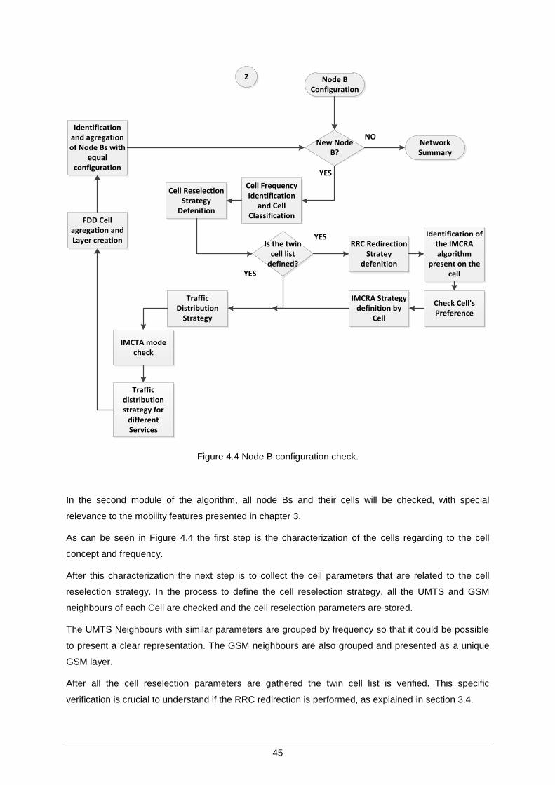
45

New Node B?

Cell Frequency Identification

and Cell Classification

Cell Reselection Strategy

Defenition

Is the twin cell list

defined?

Identification of the IMCRA algorithm

present on the cell

Check Cell's Preference

IMCRA Strategy definition by

Cell

Traffic Distribution

Strategy

IMCTA mode check

Traffic distribution strategy for

different Services

RRC Redirection Stratey

defenition

Identification and agregation of Node Bs with

equal configuration

FDD Cell agregation and Layer creation

2

NO

YES

YES

YES

Node B Configuration

Network Summary

Figure 4.4 Node B configuration check.

In the second module of the algorithm, all node Bs and their cells will be checked, with special

relevance to the mobility features presented in chapter 3.

As can be seen in Figure 4.4 the first step is the characterization of the cells regarding to the cell

concept and frequency.

After this characterization the next step is to collect the cell parameters that are related to the cell

reselection strategy. In the process to define the cell reselection strategy, all the UMTS and GSM

neighbours of each Cell are checked and the cell reselection parameters are stored.

The UMTS Neighbours with similar parameters are grouped by frequency so that it could be possible

to present a clear representation. The GSM neighbours are also grouped and presented as a unique

GSM layer.

After all the cell reselection parameters are gathered the twin cell list is verified. This specific

verification is crucial to understand if the RRC redirection is performed, as explained in section 3.4.

46

If the twin cell list is not defined for that twin cell, then the RRC redirection strategy is not determined

and jumps directly to the traffic distribution strategy identification, as it is represented in Figure 4.4.

Firstly it is necessary to understand which IMCRA solution is enabled in the cell. The activation

parameters are checked and the IMCRA solution is verified. To better represent the RRC redirection

strategies, a new cell classification is needed. For IMCRA Step 1 and Step 2 there are two distinct

ways to check the cell classification.

The RRC redirection strategy is then examined and all the parameters related to the IMCRA solution

implemented are stored. One important step is to check the frequency layer of the twin cells. This

information allows that this strategy could be represented in terms of frequency layers.

Once the RRC redirection verification is ready the last mobility feature, IMCTA, is checked. Depending

on which modes are enabled, it may be necessary to check up to 5 different traffic allocation

strategies.

After the cells from the node B are all checked, the layer summary is created. It is expected that all

cells in the same frequency layer have similar configurations and the same mobility strategies

implemented. Although it seems that some information can be lost in this step, all parameters are

saved by cell so that they can be consulted.

3

New Configuration

?

Node B configuration

design

Cell reselection strategy draw

RRC Redirection strategy

represention

Traffic distribution in DCH scheme

Network parametrisation report creation

to excel

Finish

NO

YES

Network Summary

Figure 4.5 Network Representation and parameter report creation.

47

With this representation the node B is configured by frequency layers and the network is described. All

node Bs with the same configuration are grouped together. The node B summary is presented as

follows: F1 (layer capability) + F2 (layer capability) + F3 (layer capability).

The last section of the algorithm refers to the strategies representation, and the parameters summary.

For each different node B configuration is created a graphical representation of the layers c and the

different mobility strategies implemented.

In Figure 4.5 is highlighted the four steps for the representation of each different node B configuration.

First the layer configuration is drawn. The different mobility strategies between all the layers are then

represented over the node B configuration.

In the final step of the algorithm a report with all parameters is exported to excel. It is organized by

node B configuration and for each cell the correspondent parameters are grouped by mobility feature.

4.3 User Interface and tool output

The user graphic interface to operate this tool is quite simple. It is only requested to the user to use a

search window to find the snapshot location. In Figure 4.6 is the example of the search window is

presented.

Figure 4.6 Windows interface for snapshot location.

48

During the tool’s execution a progress bar is used to indicate the status of the procedure. The

progress bar is presented in Figure 4.7.

Figure 4.7 Progress bar.

In the end of the network summary and strategies representation a window pops up with the

information that the tool as reach its end. In Figure 4.8 is an example of the finish window.

Figure 4.8 Finish window.

The tool output will be saved in the same location of the snapshot file. There outputs generated are:

graphical representation of the different node B configurations in the network and for each

configuration the representation of the strategy for the cell reselection, RRC redirection and traffic

distribution in cell DCH

As an example, in the figure 4.9 the graphical representation of one mobility strategy is presented, in

this case the cell reselection strategy. As can be observed in each layer the cell concept is presented,

CS/DATA and the frequency layer. In this case there is no interaction between the layers. This means

that the UEs are free to camp homogeneously over the layers.

Figure 4.9 Example of one graphical representation of the reselection strategy.

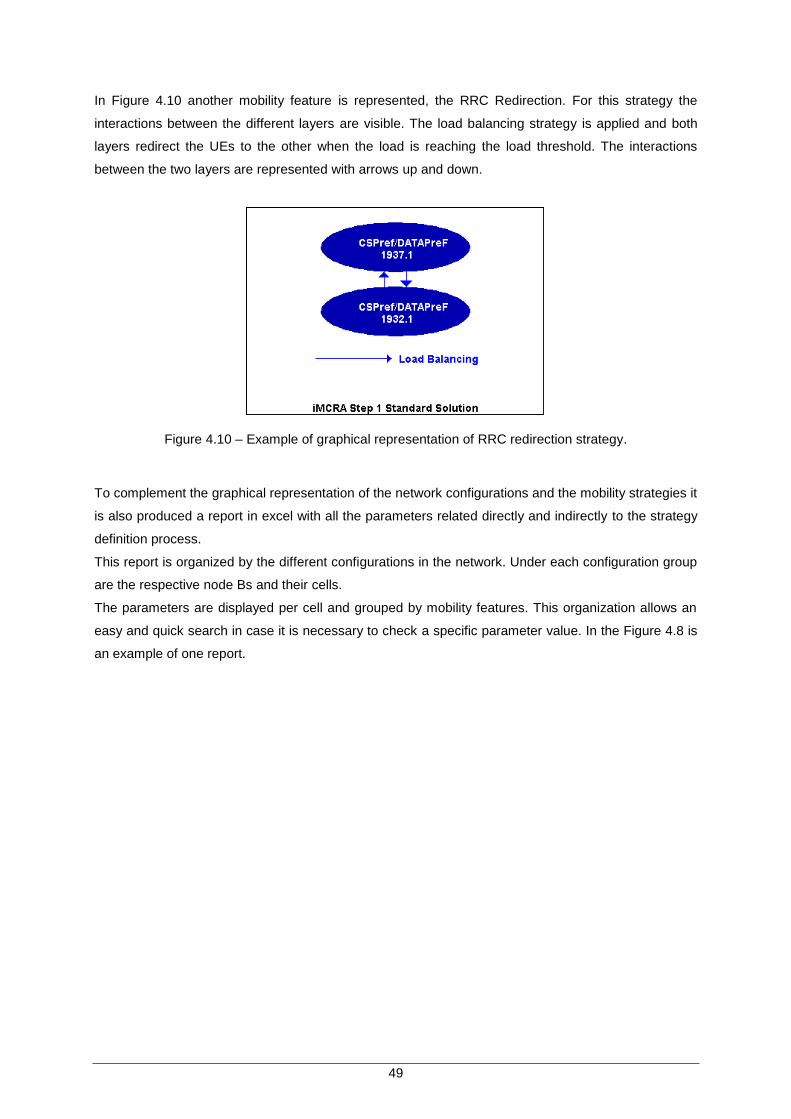
49

In Figure 4.10 another mobility feature is represented, the RRC Redirection. For this strategy the

interactions between the different layers are visible. The load balancing strategy is applied and both

layers redirect the UEs to the other when the load is reaching the load threshold. The interactions

between the two layers are represented with arrows up and down.

Figure 4.10 – Example of graphical representation of RRC redirection strategy.

To complement the graphical representation of the network configurations and the mobility strategies it

is also produced a report in excel with all the parameters related directly and indirectly to the strategy

definition process.

This report is organized by the different configurations in the network. Under each configuration group

are the respective node Bs and their cells.

The parameters are displayed per cell and grouped by mobility features. This organization allows an

easy and quick search in case it is necessary to check a specific parameter value. In the Figure 4.8 is

an example of one report.

50

Figure 4.11 Structure of the parameters report.

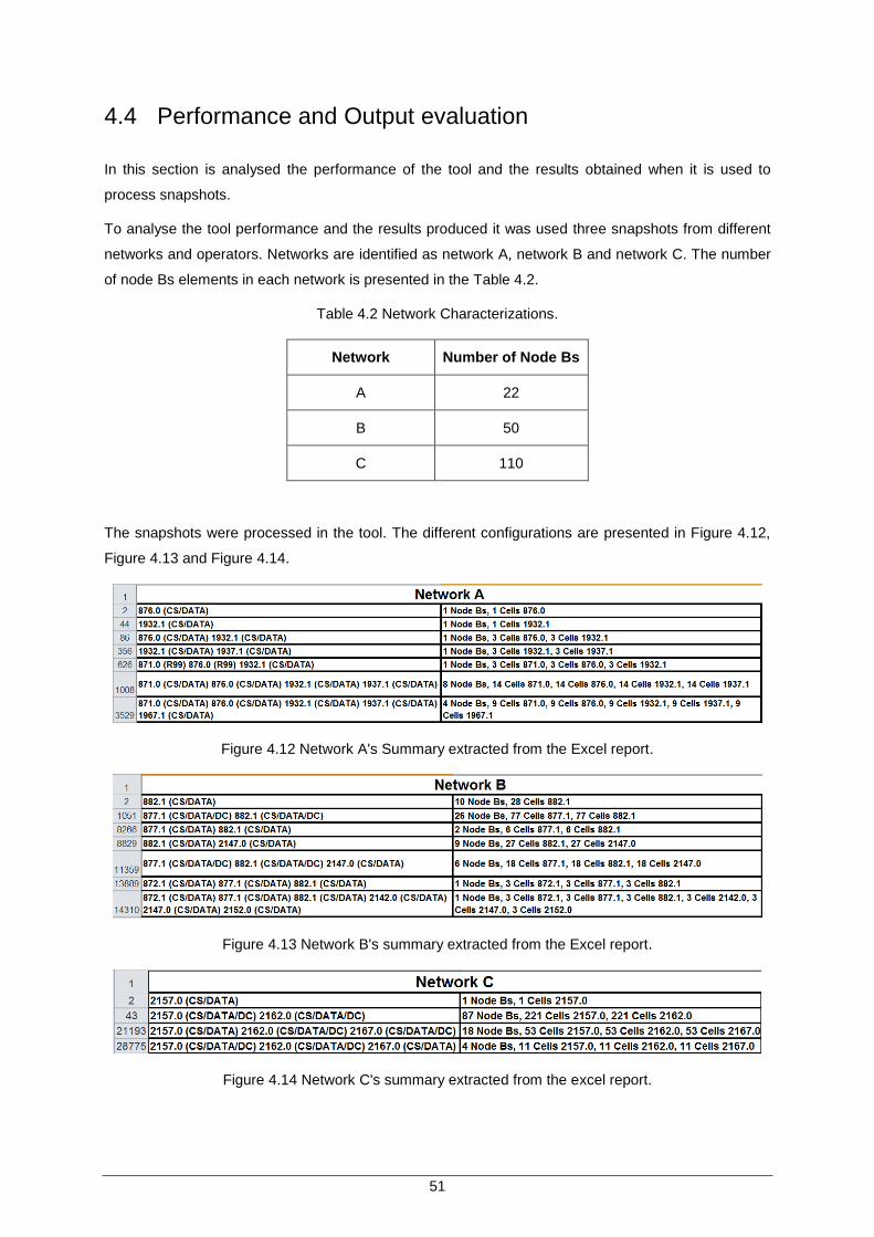
51

4.4 Performance and Output evaluation

In this section is analysed the performance of the tool and the results obtained when it is used to

process snapshots.

To analyse the tool performance and the results produced it was used three snapshots from different

networks and operators. Networks are identified as network A, network B and network C. The number

of node Bs elements in each network is presented in the Table 4.2.

Table 4.2 Network Characterizations.

Network Number of Node Bs

A 22

B 50

C 110

The snapshots were processed in the tool. The different configurations are presented in Figure 4.12,

Figure 4.13 and Figure 4.14.

Figure 4.12 Network A's Summary extracted from the Excel report.

Figure 4.13 Network B's summary extracted from the Excel report.

Figure 4.14 Network C's summary extracted from the excel report.

52

The first performance indicator to observe is the time that was spent in each network configuration

checkup. The tool took 43 seconds on the network A, 50 seconds on the network B and 124 seconds

on the network C. These values depend on the number of node Bs, number of cells in each node B

and also on the number of different configurations in the network.

On average the tool took about 1.36 seconds per node B that compared with the time spent just to

gather the parameters of one cell (20520 seconds) is approximately 15000 times faster.

From the summaries presented in Figures 4.12, 4.13, 4.14 it is possible not only to identify the

predominant configurations in each network, but to identify the unique configurations with few node

Bs. With the identification of those node Bs it is possible to perform a parameterization checkup and

discard or confirm if there is a parameterization error.

In Figure 4.13 there is an example of the case presented previously. The third configuration only has

two node Bs and they have a similar configuration to the predominant configuration, except for DC

activation. These two node Bs could be checked in order to understand if the configuration is right or if

there is a mistake.

With the network’s summary analysed, the graphical representation of the mobility strategies are used

to understand the interactions between the different layers. As an example, it will be used the

predominant strategy of the network B.

Figure 4.15 Cell Reselection strategy representation.

The Figure 4.15 presents the cell reselection strategy. The UEs camp homogeneously in the layers

8821.1 and 887.1.

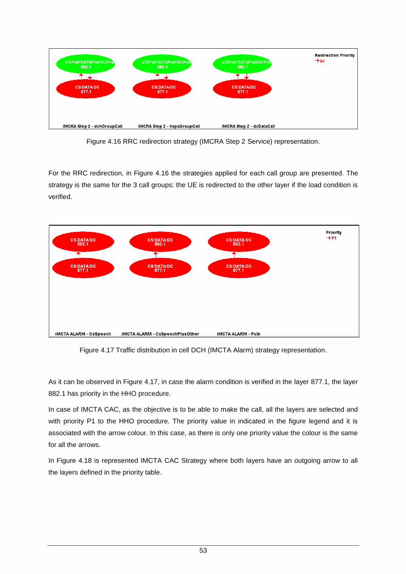
53

Figure 4.16 RRC redirection strategy (IMCRA Step 2 Service) representation.

For the RRC redirection, in Figure 4.16 the strategies applied for each call group are presented. The

strategy is the same for the 3 call groups: the UE is redirected to the other layer if the load condition is

verified.

Figure 4.17 Traffic distribution in cell DCH (IMCTA Alarm) strategy representation.

As it can be observed in Figure 4.17, in case the alarm condition is verified in the layer 877.1, the layer

882.1 has priority in the HHO procedure.

In case of IMCTA CAC, as the objective is to be able to make the call, all the layers are selected and

with priority P1 to the HHO procedure. The priority value in indicated in the figure legend and it is

associated with the arrow colour. In this case, as there is only one priority value the colour is the same

for all the arrows.

In Figure 4.18 is represented IMCTA CAC Strategy where both layers have an outgoing arrow to all

the layers defined in the priority table.

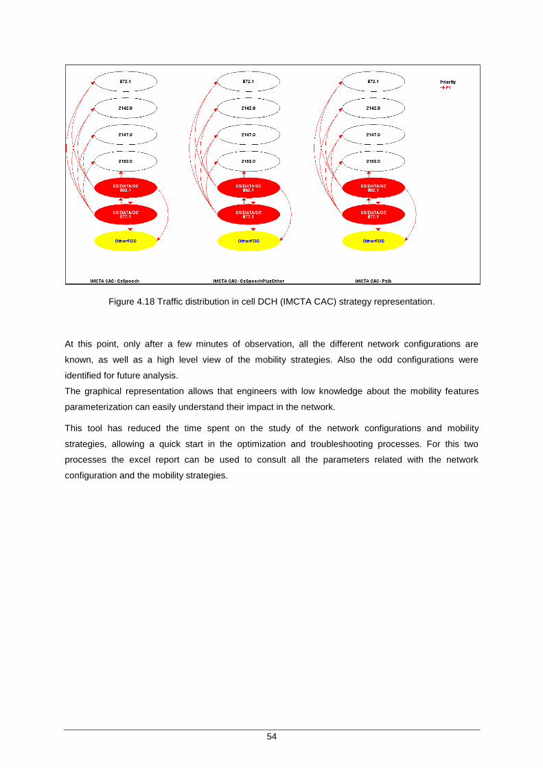
54

Figure 4.18 Traffic distribution in cell DCH (IMCTA CAC) strategy representation.

At this point, only after a few minutes of observation, all the different network configurations are

known, as well as a high level view of the mobility strategies. Also the odd configurations were

identified for future analysis.

The graphical representation allows that engineers with low knowledge about the mobility features

parameterization can easily understand their impact in the network.

This tool has reduced the time spent on the study of the network configurations and mobility

strategies, allowing a quick start in the optimization and troubleshooting processes. For this two

processes the excel report can be used to consult all the parameters related with the network

configuration and the mobility strategies.

55

Chapter 5

Conclusions and Future Works

5 Conclusions and Future Works

The main conclusions of these work and suggestions for future works are presented in this

chapter.

56

57

5.1 Conclusions

With the increase of mobile traffic due to new multimedia applications, video streaming and others,

mobile operators had to adapt, evolve and deploy new structures in the mobile networks. One of the

solutions adopted by the operators was the utilization of multi-layers networks.

To ensure a correct traffic distribution all over the different layers, traffic distribution algorithms were

also developed. To spread efficiently the traffic all over the layers there are several settings used as

decision flags for the traffic redirection namely cell capabilities, UE capabilities, call type or cell load.

Different mobility features are implemented in parallel to the network procedures. Due to constant

growth of the mobile traffic in the networks, new features were added to these algorithms. If on one

hand the constant introduction of new mobility feature improves the network efficiency, on the other

hand it also increased the network complexity.

With the increase of the network complexity and the number of new mobility features, the processes to

study the networks configurations and strategies implemented have become more complex and time

consuming. The main focus of this work was to develop one tool that automatically identifies and

resumes the different network configurations and their main mobility features.

The main mobility features from ALU UA8.1 networks were explained in the Chapter 3. The cell

reselection, the RRC redirection and the traffic distribution in cell DCH features were presented. For

each feature it was presented the main strategies.

It was also presented an high level view of the procedure to check the strategies implemented in the

network for the different mobility features.

Finally the main problems in the checkup of the strategy implemented were also identified. The time

spent in the network checkup process and the difficulty in the detection of parameterization errors

were two problems in the network checkup process. Another question identified was the difficulty into

the representation the mobility strategies implemented in the network for a quick comprehension.

As described in the Chapter 4, the network parameterisation is stored in an XML file. It was created a

database of parameters that contains all the important parameters for the mobility features. This

database has the information of the different parameter types and the parameter location in the

network.

The tool imports the parameters database as well the as the network snapshot with all the parameters

used in the network configuration. With the entire information imported the network checkup is

performed. For each cell it is identified the cell concept, the mobility features enabled and strategies

implemented in each feature.

The node Bs are then grouped by similar configuration and the different network configurations are

known, as well as the number of node Bs per configuration.

58

For the different node B configuration in the network, a graphical output is generated. In the graphical

output the different node B configuration, cell reselection, RRC redirection and traffic distribution in cell

DCH strategies are represented. With the graphical representation, the multi-layer configuration and

the mobility strategies implemented in the network are available for a high level and quick inspection.

For a closer look in the mobility strategies an excel report with all the parameters, organized by node

B configuration and mobility feature, is also created.

Finally three different networks with different number of node Bs were used to check the tool

performance. The results show that the duration of the network checkup process was reduced. The

manual procedure to collect all the parameters of one cell can take several hours. When the tool is

used, the duration of the procedure was reduced to a question of seconds.

The network summary allows us to understand the predominant configurations, and to identify the odd

ones. The graphical representation of the mobility strategies leads us to a quick understand of the

network mobility strategies, even if only in a qualitative way.

This tool allows not only to reduce the time spent in the network checkup procedure, but also allows,

with the graphical representation, that engineers with low knowledge about the mobility features

parameterization can easy understand their impact in the network.

The excel report created is also very useful in the parameter checkup, as they are all grouped together

by mobility feature.

5.2 Future Works

In this section will be presented suggestions for future works in this area.

Development of a more complex user friendly interface to allow the selection of the features

under study, as well as the selection of only some of the network elements.

Include on the algorithm other procedures besides mobility such as always-on and HSPA.

Introduce key performance indicator analysis feature to understand how the parameters

changes have impact in the network procedures and to create a representation of the UE

distribution all over the different layer and for the different mobility procedures.

59

Annex A

Parameters type format and

XML Structure

Annex A. Parameters Type and XML Structures

To generate the XML file with the parameter database it was created a VBA macro to convert the

content of an excel file to a XML file. In this annex de different parameters configurations in the excel

file and the output generated for each parameter type is shown.

60

61

A.1 Parameters Fields

The database of parameters contains all the parameters that needed to be imported to the tool. Each

parameter, depending on its type has different attributes and formats. Due to this situation, it is

necessary to classify the different parameters configuration and the XML structure use in the tool.

The fields needed to be fill in the excel file are presented in the Figure A.1

Figure A.1 Fields used in the parameter characterization.

The Name is the field for the name of the parameter. This name must be exactly the same as the one

set in the tool, to avoid having fields missed while importing the snapshot.

The second filed is the type. This will be field with Number, Enum, Boolean, Pointer, IntList and

Binary. In the Path, the path to the location of the object is stated.

The Values field is the one that have different configurations considering the parameter type. This field

will be explained in the following paragraph for each parameter type.

In case the parameter has a default value, it will be defined in the Default field. The feature Id is

defined in the field Feature and for the parameters that are activation flags, the field isActivationFlag is

set. The field reservedField, bitRange, Type2 and Values2 are only use for the binary type and will be

explained later in this annex.

A.2 Parameter type configuration and XML file structure

Each parameter type has different attributes and different configurations. In this section the

configuration of each parameter type and the correspondent XML structure is presented. The layout of

the XML file is also presented.

Number

In case the parameter is a Number, the Values field has three attributes, minimum value, maximum

value and step. The values are split with the character “|”.An example is presented in Figure C.2. In

this case the minimum value is 1, the maximum value is 999 and the step is 1.

Name Type Path Values Default Feature IsActivationFlag reservedField bitRange Type2 Values2

62

Figure A.2 Configuration of the field Value for one parameter type Number

The XML structure of one parameter type number is shown in Figure C.3. In the sub-tal Attributes are

defined three sub-tags:, Vmin which contains the minimum value , the Vmax which contains the

maximum number and the Step with the step value.

Figure A.3 XML structure of a parameter type Number.

Pointer

The parameter type Pointer has a simple configuration. In this case the field Values is left empty. It is

only necessary to insert the parameter name, parameter type and the path in the snapshot

The XML structure of one parameter type Pointer is shown in Figure C.4. The XML structure only has

information of the path and the feature identification number.

Figure A.4 XML structure of a parameter type number.

Values

1|999|1|

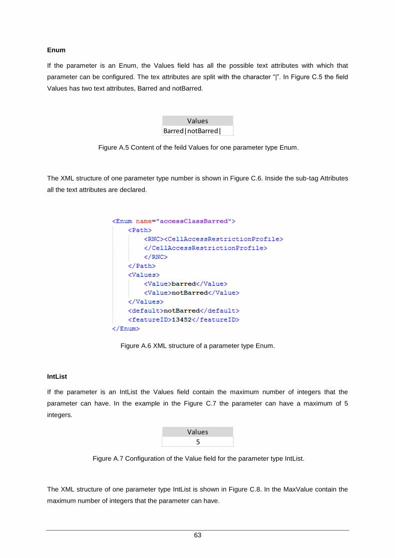
63

Enum

If the parameter is an Enum, the Values field has all the possible text attributes with which that

parameter can be configured. The tex attributes are split with the character “|”. In Figure C.5 the field

Values has two text attributes, Barred and notBarred.

Figure A.5 Content of the feild Values for one parameter type Enum.

The XML structure of one parameter type number is shown in Figure C.6. Inside the sub-tag Attributes

all the text attributes are declared.

Figure A.6 XML structure of a parameter type Enum.

IntList

If the parameter is an IntList the Values field contain the maximum number of integers that the

parameter can have. In the example in the Figure C.7 the parameter can have a maximum of 5

integers.

Figure A.7 Configuration of the Value field for the parameter type IntList.

The XML structure of one parameter type IntList is shown in Figure C.8. In the MaxValue contain the

maximum number of integers that the parameter can have.

Values

Barred|notBarred|

Values

5

64

Figure A.8 XML structure of a parameter type number.

Boolean

Similar with the Pointer, the parameter type Boolan don’t have any value in the Values field. The tool

nows that in this case the parameter has the attribute true or false.

The XML structure of one parameter type number is shown in Figure C.10. As it can be observed the

XLM structure does not have the sub-tag Attributes.

Figure A.9 XML structure of a parameter type number.

Binary

Finally the parameter type Binary is presented. The configuration of this parameter is more complex

compared with the other parameter types because we have to match the different binary

configurations with the real parameter values.

In Figure C.11 we have a configuration example. In the field Values is the possible binary

configurations for the parameter. In this case it can be 0 or 1.

The reservedField field has the information of name of the parameter in the snapshot that has the

binary information. The bitRange field indicate us which are the bits that need to be considered for the

analysis. In this case as we only have on bit, the bitRange start and finish in the same bit, 20. The last

two fields contain the parameter type that the Binary parameter is representing and the values that the

binary configuration maps. In this case if the bit 20 is 0 it means that the Boolean parameter is false,

and if the is 1 the parameter is true.

65

Figure A.10 Configuration of the parameter type Binary.

Figure A.11 XML structure of a parameter type number.

An example of the XML structure of this parameter type is presented in Figure C11. Inside the sub-tag

bitRange we have two sub-tags: Ibit that contain the number of the initial bit to be considered and Ebit

that contain the number of the last bit to be considered.

In the sub-tag Configuration are the different bit configurations. The sub-tag PmType has the true

parameter type that is being represented in the reserved parameter and the Values sub-tag contain

the possible values that this parameters can have.

XML file layout

The XML file structure is very simple. It starts with the tag <RMD> and end with the correspondent

closing tag </RMD>.

Values Default Feature IsActivationFlag reservedField bitRange Type2 Values2

0|1| 0 89857 reserved0 20|20| Boolean false|true|

66

67

References

References

[1] Correia, L. M., Mobile Broadband Multimedia Networks. Elsevier Ltd, Oxford. UK 2006

[2] Hola, H. and Toskala .A., WCDMA for UMTS – HSPA Evolution and LTE, 4th Edition, John Wiley &

Sons, UK. 2007

[3] 4G Americas, Global Deployment Status Update, October 2013

[4] Alcatel-Lucent, “UTRAN Parameter User Guide UA08”, Ver. 13.05, November 2012

[5] ETSI, Universal Mobile Telecommunications System (UMTS); Base Station (BS) radio transmission

and reception (FDD), Technical Specification 125.104, Ver. 11.5.0, April 2013

[6] Alcatel-Lucent, “9300 W-CDMA UA07 R99 Radio Principles”, Student Guide, Alcatel-Lucent

University 2010. (Internal Document)

[7] 3GPP, Technical Specification Group Services and System Aspects General UMTS Architecture,

Technical Specification 23.101, Ver. 3.1.0, December 2000

[8] 3GPP, Universal Mobile Telecommunications System (UMTS); Physical Layer; Measurements

(FDD), Technical Specification 25.215, Ver. 11.0.0, June 2002

[9] 3GPP, Technical Specification Group Services and Radio Access Network; UTRAN Overall

Description (Release 1999), Technical Specification 25.401, Ver. 30.1.0, November 2012

[10] 3GPP, Technical Specification group Radio Access Network; Radio Resource Control (RRC);

protocol specification (Release 11), Technical Specification 25.331, Ver. 11.5.0, April 2012

[11] Alcatel-Lucent, “UTRAN Performance Monitoring Guidelines UA08”, August 2012 (Internal

document)

[12] Alcatel-Lucent, “9300 W-CDMA TMO18255 UA07 R99 Algorithm Description”, Alcatel-Lucent

University, 2010 (Internal Document)

[13] 3GPP, Universal Mobile Telecommunications Systems (UMTS); UE Radio Access capabilities,

Version 8.12.0, July 2011

[14] Alcatel-Lucent, HSxPA Parameters User Guide UA08.01, V05.05, November 2012