3G Meets the Internet: Understanding

the Performance of Hierarchical

Routing in 3G Networks

Wei Dong (U T Austin)Joint work with

Zihui Ge, Seungjoon Lee

(AT&T Labs - Research)

ITC 2011, San Francisco, USA

September 2011

Outline

� Background

� Hierarchical routing vs. flat routing

� Hierarchical routing and replicated service

� Possible interaction with application layer

Summary

2

� Summary

Why do we care about 3G performance

3

3G networks now carry more traffic than ever beforeUser’s expectation on 3G performance is higher than

ever before

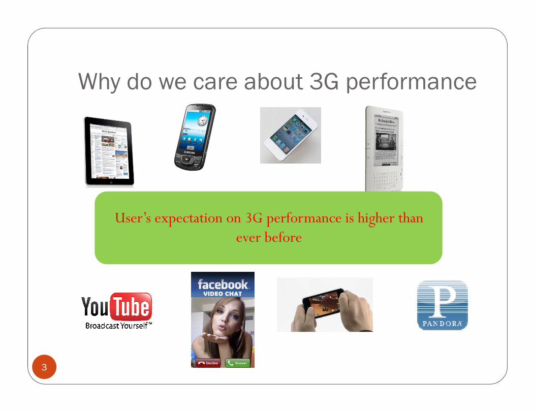
Simplified 3G Architecture

User Device

Node B

SGSN

GGSN

4

User Device

Node B

RNC

GGSN

Destination

A

C

B

Outline

� Background

� Hierarchical routing vs. flat routing

� Hierarchical routing and replicated service

� Possible interaction with application layer

Summary

5

� Summary

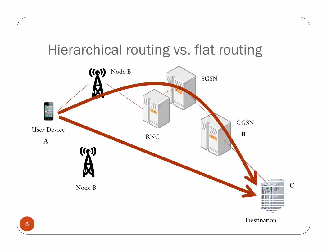
Hierarchical routing vs. flat routing

User Device

Node BSGSN

GGSN

6

User Device

Node B

RNC

GGSN

Destination

A

C

B

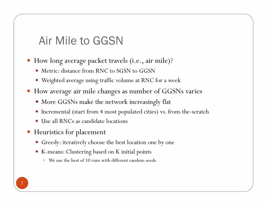
Air Mile to GGSN

� How long average packet travels (i.e., air mile)?

� Metric: distance from RNC to SGSN to GGSN

� Weighted average using traffic volume at RNC for a week

� How average air mile changes as number of GGSNs varies

� More GGSNs make the network increasingly flat

7

� More GGSNs make the network increasingly flat

� Incremental (start from 4 most populated cities) vs. from-the-scratch

� Use all RNCs as candidate locations

� Heuristics for placement

� Greedy: iteratively choose the best location one by one

� K-means: Clustering based on K initial points

� We use the best of 10 runs with different random seeds

800

1000

1200

1400Av

erag

e D

ista

nce

(km

)

Greedy from existingGreedyK−meansLower bound

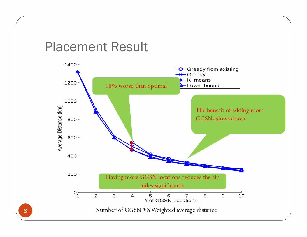
Placement Result

18% worse than optimal

The benefit of adding more

GGSNs slows down

1 2 3 4 5 6 7 8 9 100

200

400

600

800

# of GGSN Locations

Aver

age

Dis

tanc

e (k

m)

8 Number of GGSN VSWeighted average distance

GGSNs slows down

Having more GGSN locations reduces the air

miles significantly

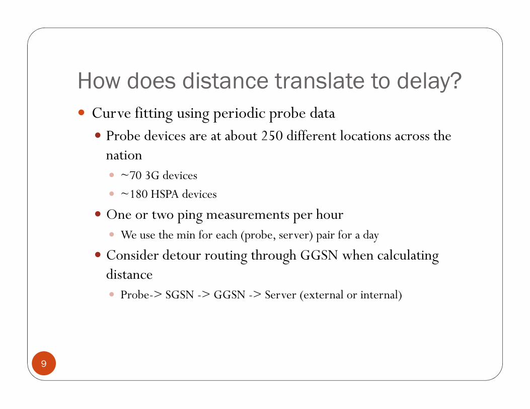
How does distance translate to delay?

� Curve fitting using periodic probe data

� Probe devices are at about 250 different locations across the

nation

� ~70 3G devices

� ~180 HSPA devices

9

� One or two ping measurements per hour

� We use the min for each (probe, server) pair for a day

� Consider detour routing through GGSN when calculating

distance

� Probe-> SGSN -> GGSN -> Server (external or internal)

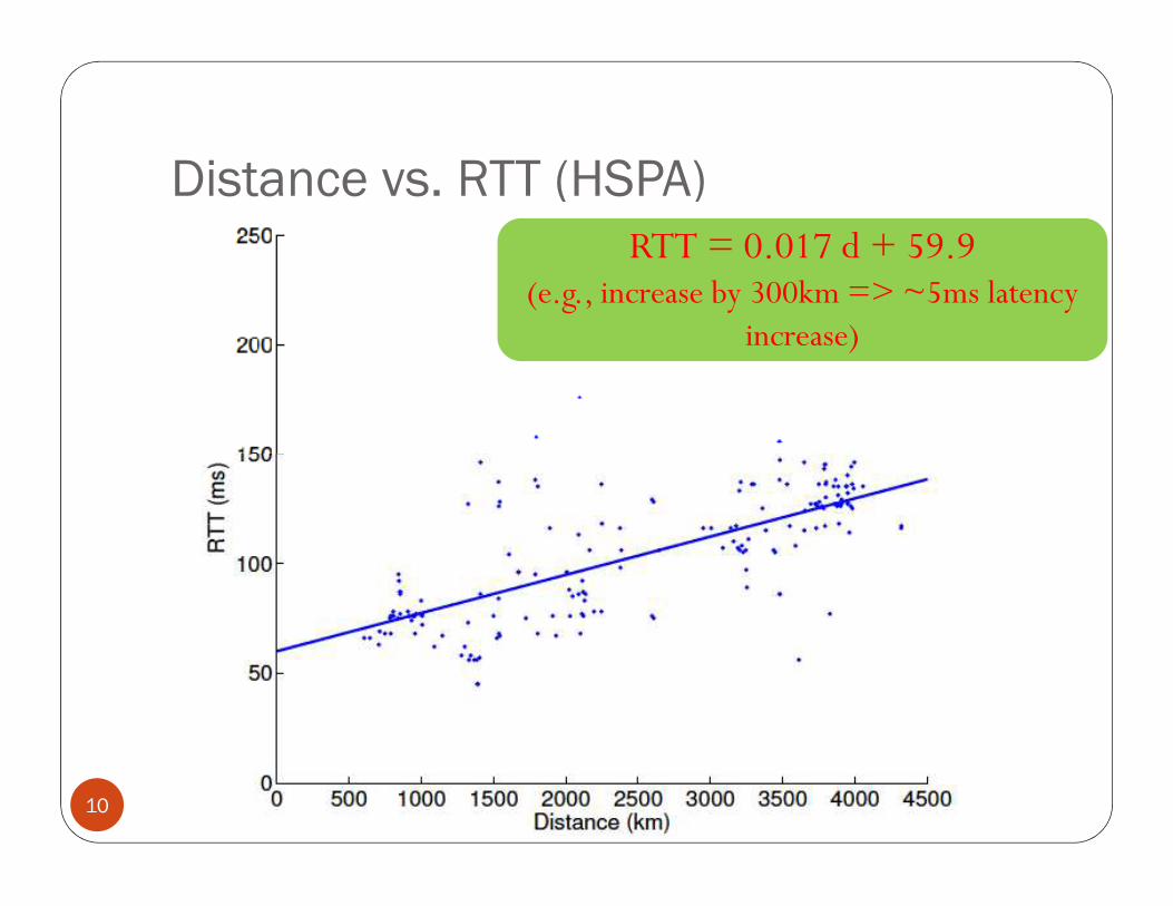
Distance vs. RTT (HSPA)

RTT = 0.017 d + 59.9(e.g., increase by 300km => ~5ms latency

increase)

10

Outline

� Background

� Hierarchical routing vs. flat routing

� Hierarchical routing and replicated service

� Possible interaction with application layer

Summary

11

� Summary

Hierarchical routing and replicated

service

User Device

Node BSGSN

GGSN

A

12

Node B

RNC

GGSN

Destination

C

B

D

With CDN, relative

performance is even worse!

Hierarchical routing and replicated

service� Air mile to CDN server (weighted average)� EAG (Exit-at-GGSN): Current routing� RNC – SGSN – GGSN – CDN server

� EAS, EAR (Exit at SGSN/RNC): idealized routing� RNC – SGSN – CDN or RNC – CDN

� CDN server selection

13

� CDN server selection

� Normal: closest to exit point

� DNS caching can cause suboptimal selection (discussed later)

� Location information� RNC (hundreds of different locations), SGSN (tens of different

locations), GGSN (tens of different locations)� Location of CDN servers (tens of different locations)

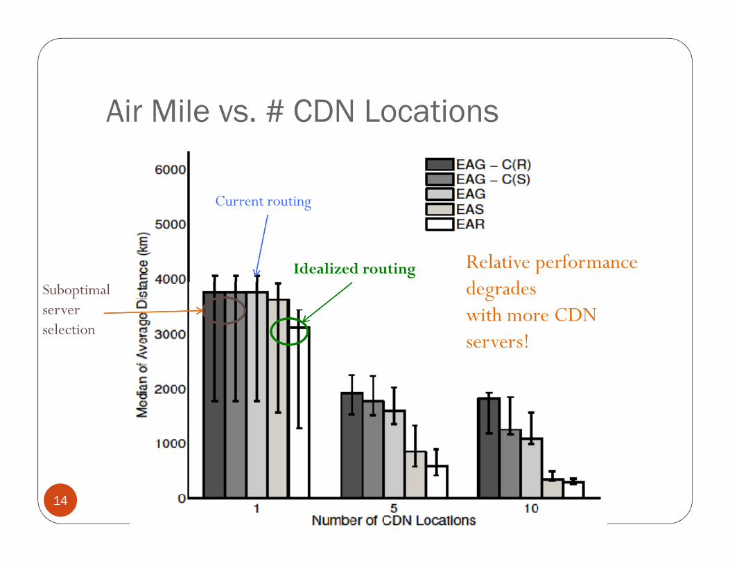
Air Mile vs. # CDN Locations

Current routing

Idealized routing

Suboptimal

Relative performance

degrades

14

Suboptimal

server

selection

degrades

with more CDN

servers!

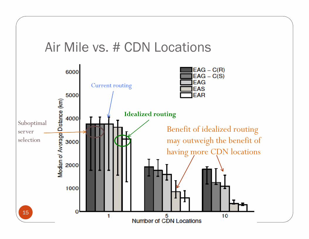
Air Mile vs. # CDN Locations

Current routing

Idealized routing

Suboptimal

15

Suboptimal

server

selection

Benefit of idealized routing

may outweigh the benefit of

having more CDN locations

Distance Distribution (tens of CDN

Locations)

0.6

0.7

0.8

0.9

1

Difference of median is

851 km which translates to

23.7% difference in RTT

16

0 500 1000 1500 2000 2500 3000 3500 4000 45000

0.1

0.2

0.3

0.4

0.5

Distance (km)

CD

F

Current

Exit at SGSN

Exit at RNC

CDF of Distance

Outline

� Background

� Hierarchical routing vs. flat routing

� Hierarchical routing and replicated service

� Possible interaction with application layer

Summary

17

� Summary

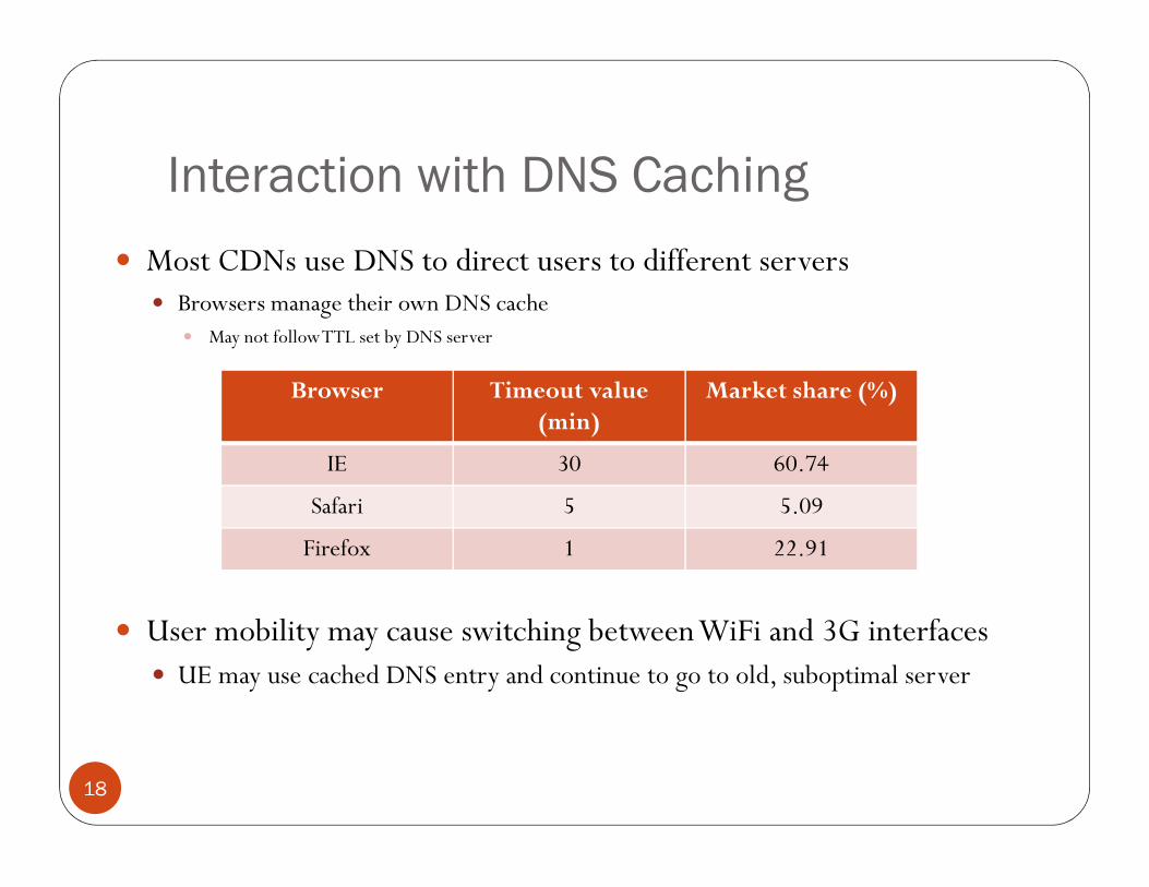
Interaction with DNS Caching

� Most CDNs use DNS to direct users to different servers� Browsers manage their own DNS cache

� May not follow TTL set by DNS server

Browser Timeout value

(min)

Market share (%)

18

� User mobility may cause switching between WiFi and 3G interfaces

� UE may use cached DNS entry and continue to go to old, suboptimal server

IE 30 60.74

Safari 5 5.09

Firefox 1 22.91

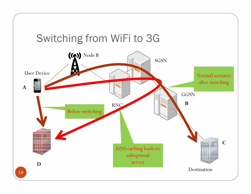
Switching from WiFi to 3G

User Device

Node BSGSN

GGSN

Normal scenario

after switchingA

19

RNC

GGSN

Destination

Before switching

DNS caching leads to

suboptimal

server

C

B

D

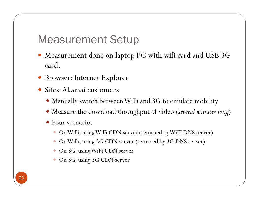
Measurement Setup

� Measurement done on laptop PC with wifi card and USB 3G

card.

� Browser: Internet Explorer

� Sites: Akamai customers

� Manually switch between WiFi and 3G to emulate mobility

20

� Manually switch between WiFi and 3G to emulate mobility

� Measure the download throughput of video (several minutes long)

� Four scenarios

� On WiFi, using WiFi CDN server (returned by WiFI DNS server)

� On WiFi, using 3G CDN server (returned by 3G DNS server)

� On 3G, using WiFi CDN server

� On 3G, using 3G CDN server

0.2

0.25

0.3

0.35

0.4

3G to 3G-

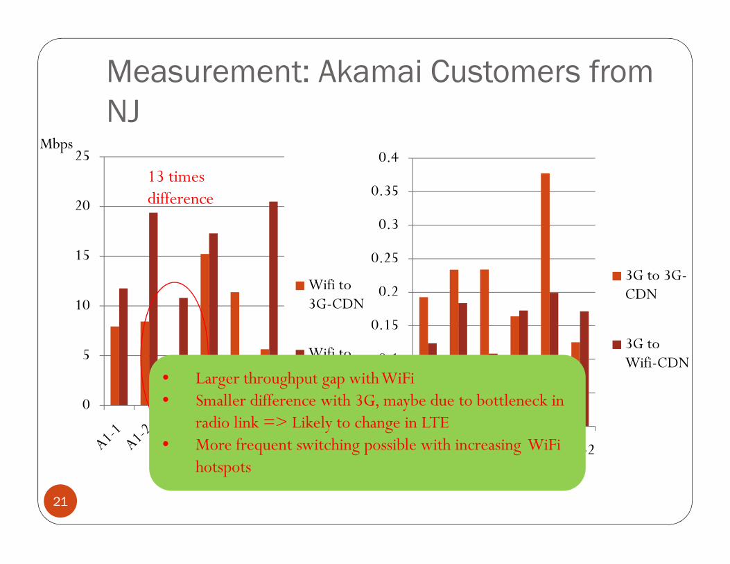
Measurement: Akamai Customers from

NJ

15

20

25

Wifi to

Mbps

13 times

difference

0

0.05

0.1

0.15

0.2

A1-1A1-2A2-1A2-2A3-1A3-2

3G to 3G-CDN

3G to Wifi-CDN

21

0

5

10

Wifi to 3G-CDN

Wifi to Wifi-CDN

WiFi 3G

• Larger throughput gap with WiFi

• Smaller difference with 3G, maybe due to bottleneck in

radio link => Likely to change in LTE

• More frequent switching possible with increasing WiFi

hotspots

Summary

� Compared between idealized routing and current detour routing in 3G architecture� Flat routing reduces air mile significantly but the difference in

end-to-end delay is only modest

� Relative performance gap grows with replicated service

� Interaction between routing change and DNS caching can cause

22

� Interaction between routing change and DNS caching can cause up to an order of magnitude throughput degradation

� Our findings not only apply to current 3G networks

� The difference in end-to-end delay can grow as wireless technology improves further

� The use of aggregation points still applies to recent cellular architectures such as EPC

Q&A

Thanks!

23

Backup Slides

24

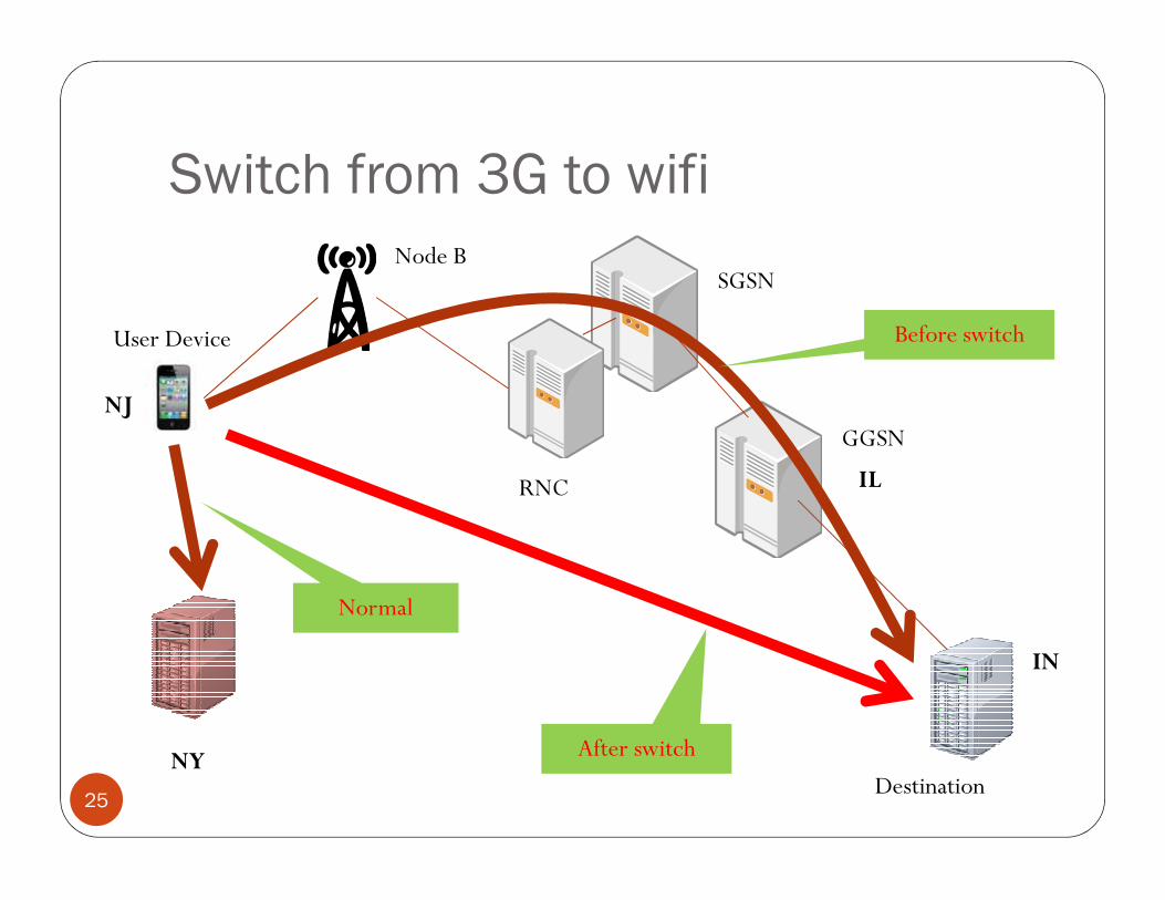
Switch from 3G to wifi

User Device

Node BSGSN

GGSN

Before switch

NJ

25

RNC

GGSN

Destination

Normal

After switch

IN

IL

NY

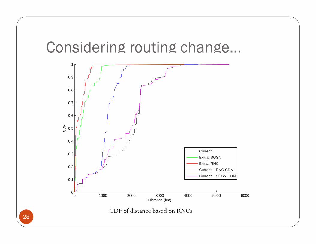
Considering routing change…

0.6

0.7

0.8

0.9

1C

DF

Over 1600 km!

26

0 1000 2000 3000 4000 5000 60000

0.1

0.2

0.3

0.4

0.5

Distance (km)

CD

F

Current

Exit at SGSN

Exit at RNC

Current − RNC CDN

Current − SGSN CDN

CDF of Distance

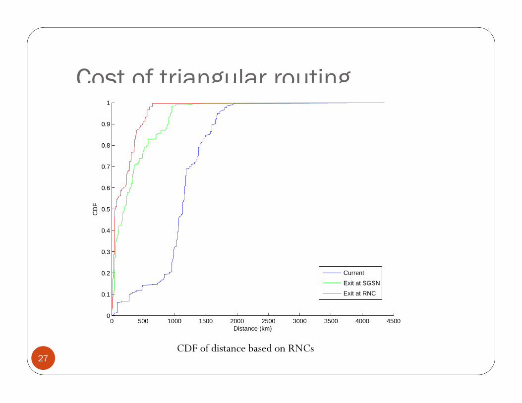
Cost of triangular routing

0.6

0.7

0.8

0.9

1C

DF

27

0 500 1000 1500 2000 2500 3000 3500 4000 45000

0.1

0.2

0.3

0.4

0.5

Distance (km)

CD

F

Current

Exit at SGSN

Exit at RNC

CDF of distance based on RNCs

Considering routing change…

0.6

0.7

0.8

0.9

1

28

0 1000 2000 3000 4000 5000 60000

0.1

0.2

0.3

0.4

0.5

Distance (km)

CD

F

Current

Exit at SGSN

Exit at RNC

Current − RNC CDN

Current − SGSN CDN

CDF of distance based on RNCs

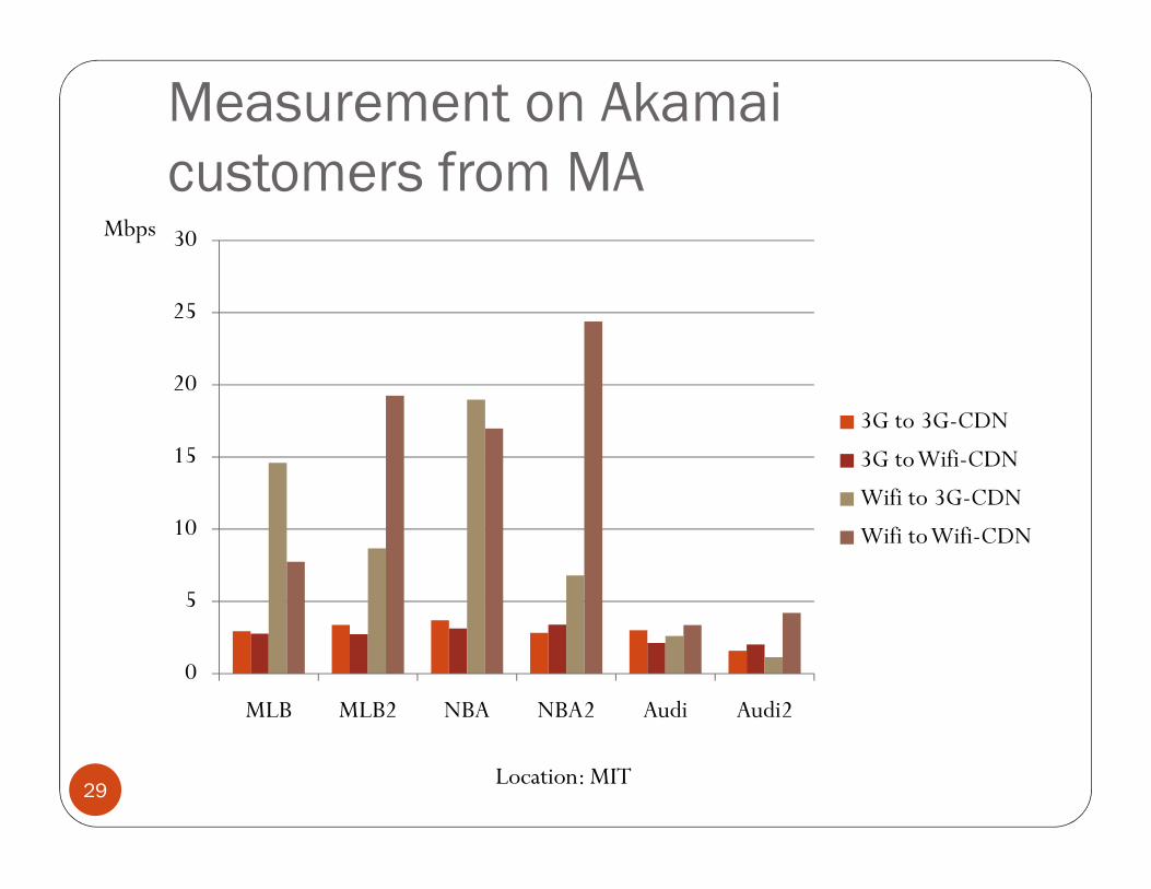
Measurement on Akamai

customers from MA

15

20

25

30

3G to 3G-CDN

3G to Wifi-CDN

Mbps

29

0

5

10

15

MLB MLB2 NBA NBA2 Audi Audi2

3G to Wifi-CDN

Wifi to 3G-CDN

Wifi to Wifi-CDN

Location: MIT

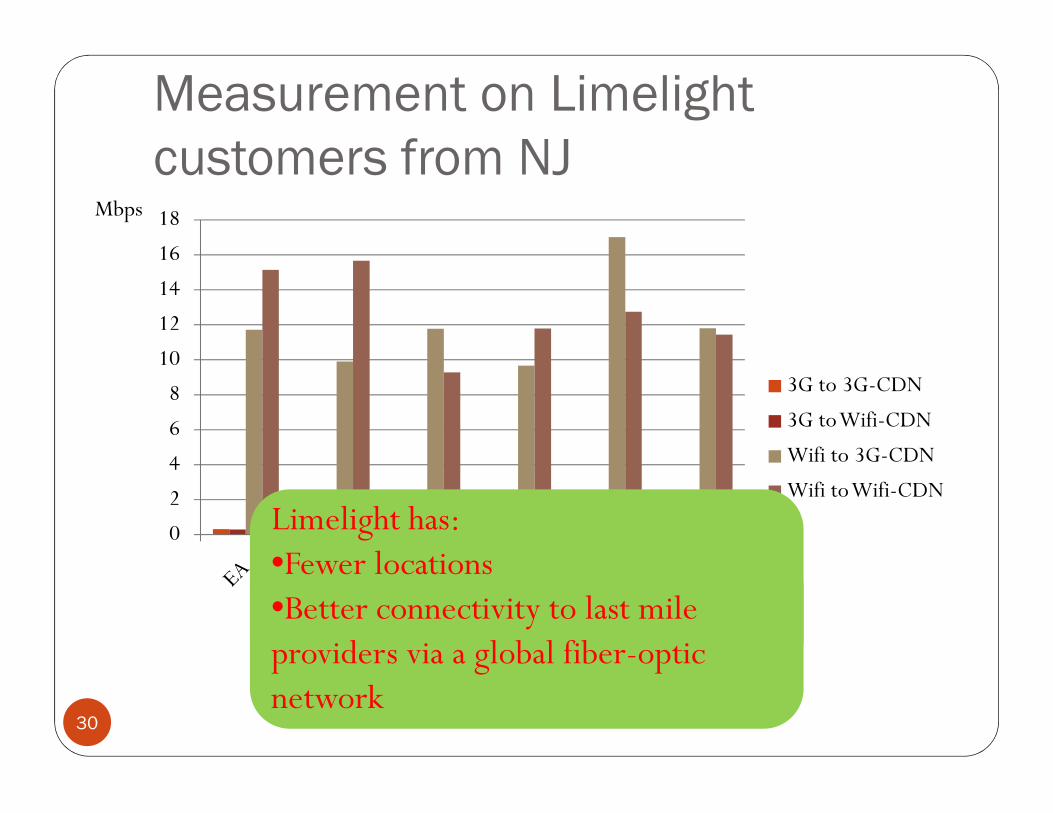
Measurement on Limelight

customers from NJ

8

10

12

14

16

18

3G to 3G-CDN

3G to Wifi-CDN

Mbps

30

0

2

4

6

83G to Wifi-CDN

Wifi to 3G-CDN

Wifi to Wifi-CDN

Inefficiency is less obvious. Why?

Location: AT&T Labs

Limelight has:

•Fewer locations•Better connectivity to last mile providers via a global fiber-optic

network

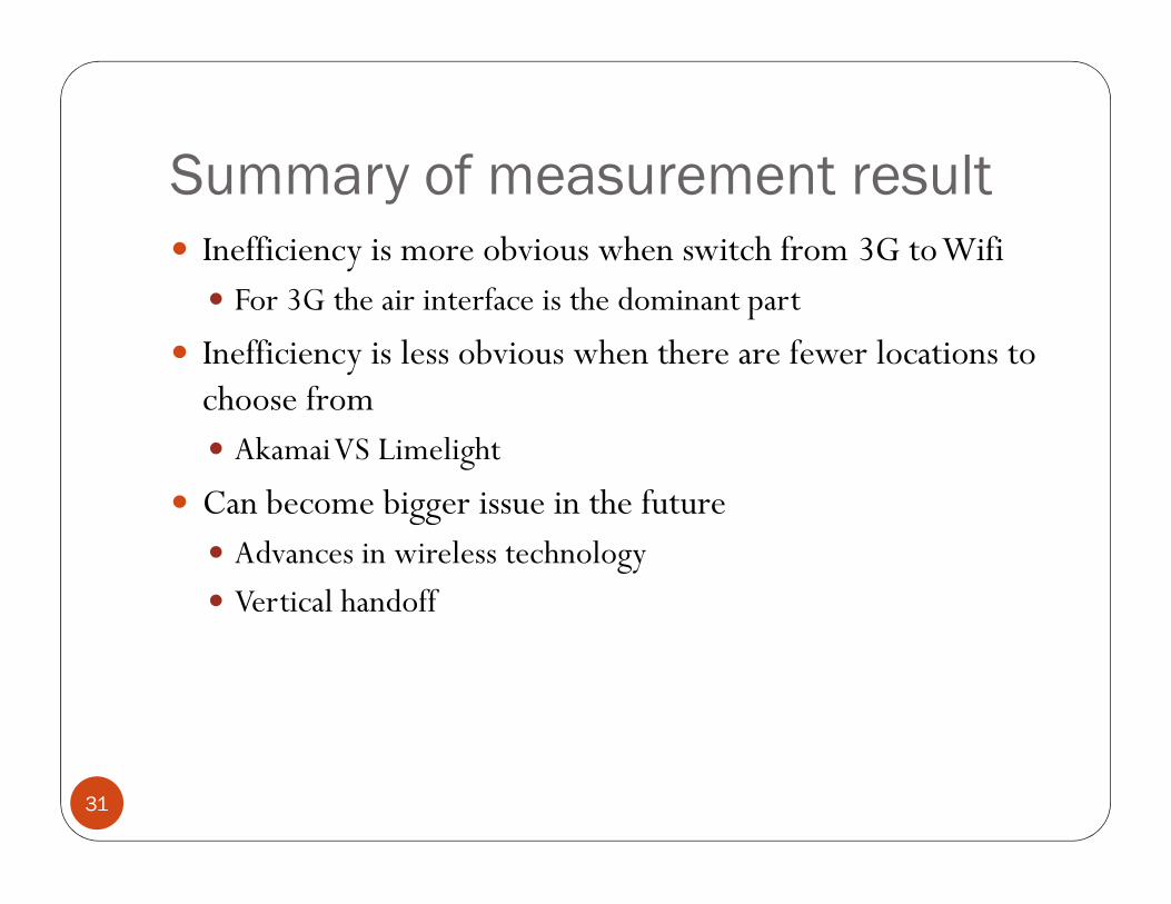
Summary of measurement result

� Inefficiency is more obvious when switch from 3G to Wifi

� For 3G the air interface is the dominant part

� Inefficiency is less obvious when there are fewer locations to

choose from

� Akamai VS Limelight

31

� Akamai VS Limelight

� Can become bigger issue in the future

� Advances in wireless technology

� Vertical handoff

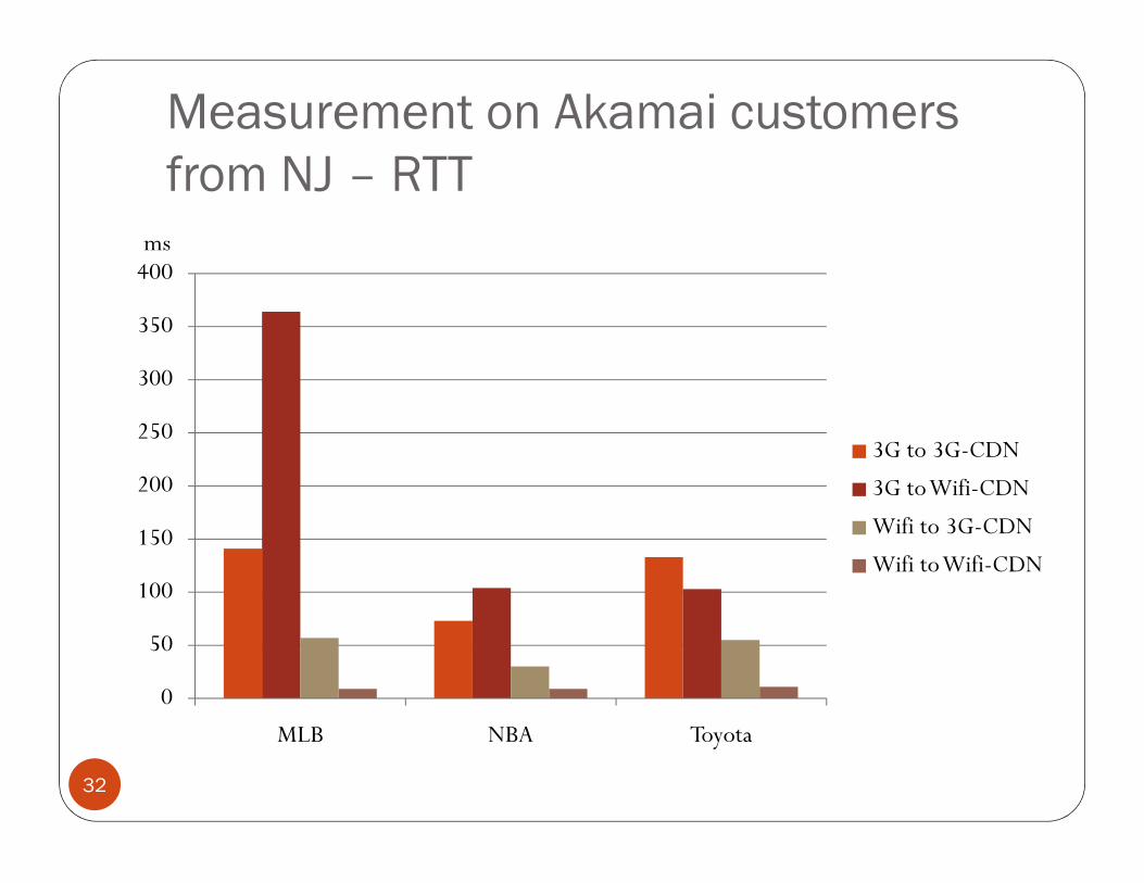
Measurement on Akamai customers

from NJ – RTT

250

300

350

400

3G to 3G-CDN

ms

32

0

50

100

150

200

250

MLB NBA Toyota

3G to 3G-CDN

3G to Wifi-CDN

Wifi to 3G-CDN

Wifi to Wifi-CDN