Embed Size (px)
Citation preview
4 Filter Analysis and Design
Filtering, the ability to selectively suppress or enhance particular parts of a signal, is perhaps
the most important tool for signal processing. Signals and Systems meets this need byproviding representations of rational pole-zero filters in both the continuous (analog) anddiscrete (digital) domains. Routines to transform a filter from analog to discrete-time areprovided, as are the most common analog filter prototypes.
While general nonlinear filters or design tools for multidimensional filters are not yet directly
supported by these routines, there are some special routines for designing two-dimensionaldecimation systems. They do not yet assist in the design of the filter itself, but they canproduce optimal decimation systems for a given passband specification with rectangularsampling.
As per usual convention, discrete-time filter design is also referred to as digital filter design in
this chapter and in Signals and Systems in general.
à 4.1 Analog Filter Design
The most common representation for a rational filter is in terms of the poles and zeros of thesystem function. Signals and Systems employs this in the AnalogFilter object.
AnalogFilter@8p1, p2, …<,8z1, z2, …<, varD an analog pole-zero filter for poles pn and zeros zn in the time variable var
Representing analog filters.
The AnalogFilter object is the basic object in this application for representing an analog
filter. Other tools are described later on that allow you to derive an analog filter in terms of
standard design classes (e.g., Bessel filters, elliptic filters, etc.). The filter object acts as aSignals and Systems operator; to determine the impulse response, you apply the filter to animpulse, and use the analysis tools to convert the system into a functional or graphical form.
Printed by Mathematica for Students
† First, make the functions available for use.
In[1]:= Needs["SignalProcessing`"]
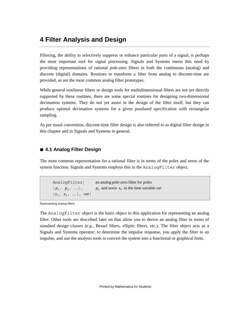
† Here is a stable analog filter. Remember that the poles of the filter's transfer function are given first, then the zeros.
In[2]:= filt = AnalogFilter[ {-.3, -.2 + .7 I, -.2 - .7 I}, {0, .2, -.2 }, t];
† The filter object normally acts in the same fashion as other operators. To determine the response of the filter to a signal, the filter object should be applied to the signal and evaluated. Here is the impulse response of our sample filter.
In[3]:= EvaluateOperators[ filt[DiracDelta[t]]]
Out[3]= 1. DiracDelta@tD − H0.03 − 1.18161×10⁻¹⁹ L −0.3 t UnitStep@tD −H0.335 + 0.245 L H−0.2−0.7 L t UnitStep@tD −H0.335 − 0.245 L H−0.2+0.7 L t UnitStep@tD† We can plot the computed response.
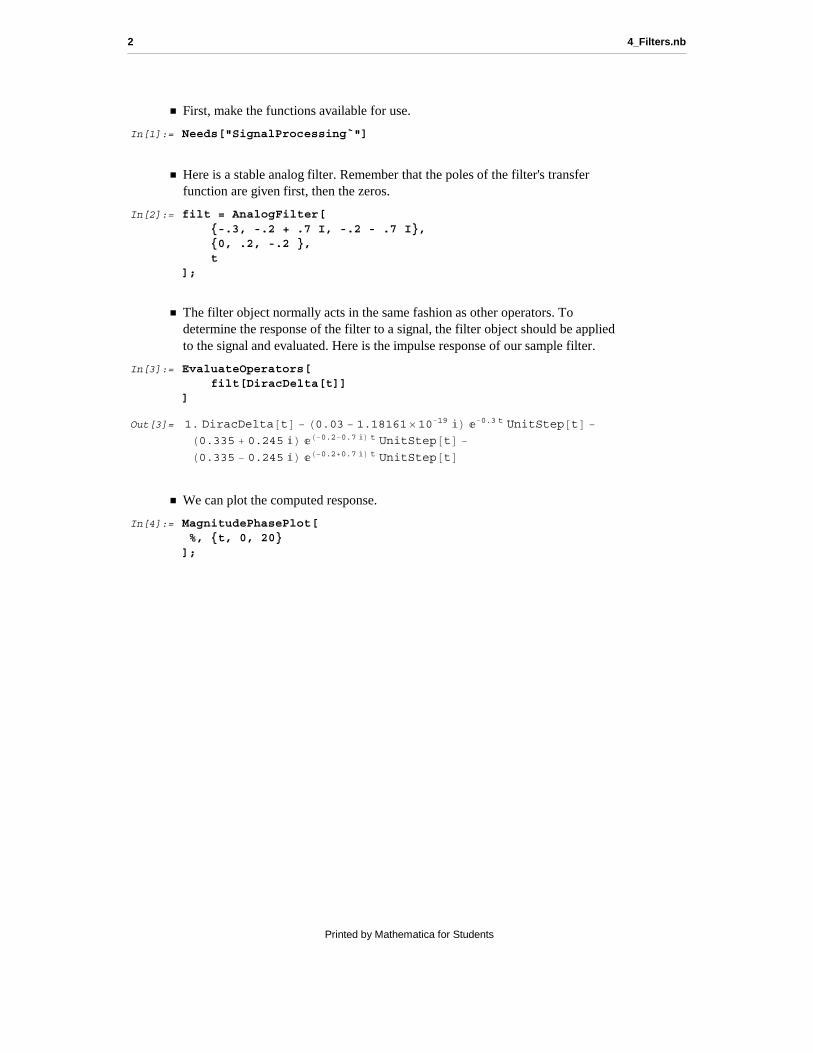
In[4]:= MagnitudePhasePlot[ %, {t, 0, 20}];
2 4_Filters.nb
Printed by Mathematica for Students
5 10 15 20t
0.1
0.2
0.3
0.4
0.5
0.6
0.7
Magnitude Response
5 10 15 20t
25
50
75
100
125
150
175
Phase Response HdegreesL
† Unlike other operators, certain functions can act solely on the filter object. For instance, here is a Laplace transform of the object, which returns the system transfer function with information about the region of convergence.
In[5]:= LaplaceTransform[filt, t, s]
Out[5]= LaplaceTransformDataA H−0.2 + sL s H0.2 + sLHH0.2 − 0.7 L + sL HH0.2 + 0.7 L + sL H0.3 + sL ,
RegionOfConvergence@−0.2, ∞D, TransformVariables@sDE
4_Filters.nb 3
Printed by Mathematica for Students
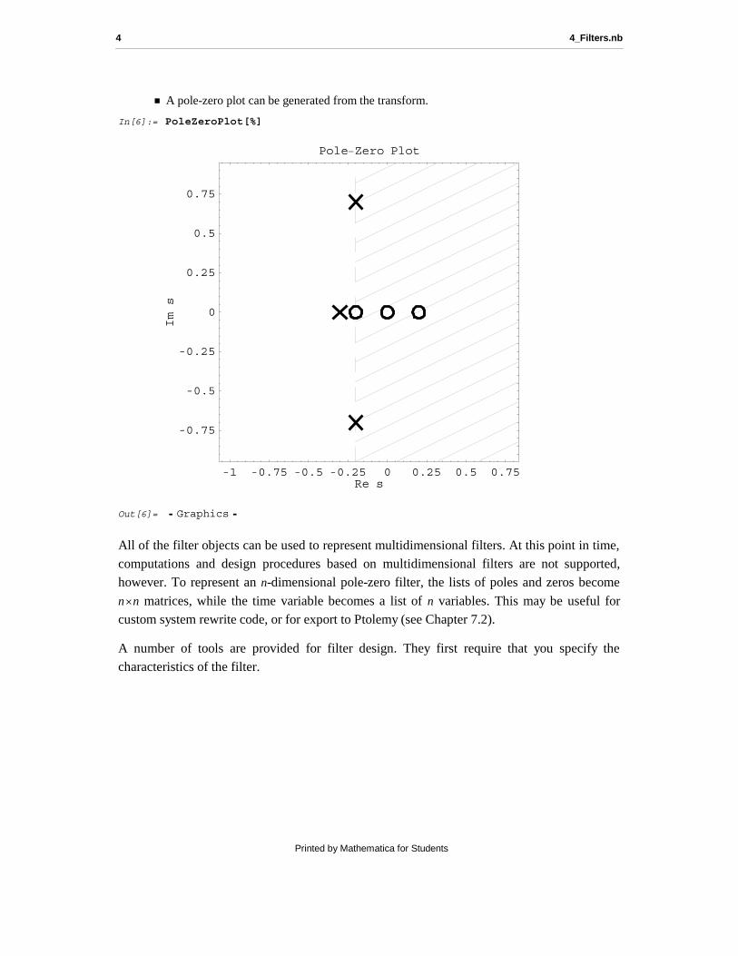
† A pole-zero plot can be generated from the transform.
In[6]:= PoleZeroPlot[%]
-1 -0.75 -0.5 -0.25 0 0.25 0.5 0.75Re s
-0.75
-0.5
-0.25
0
0.25
0.5
0.75
mI
s
Pole−Zero Plot
Out[6]= Graphics
All of the filter objects can be used to represent multidimensional filters. At this point in time,computations and design procedures based on multidimensional filters are not supported,however. To represent an n-dimensional pole-zero filter, the lists of poles and zeros become
nän matrices, while the time variable becomes a list of n variables. This may be useful forcustom system rewrite code, or for export to Ptolemy (see Chapter 7.2).
A number of tools are provided for filter design. They first require that you specify thecharacteristics of the filter.
4 4_Filters.nb
Printed by Mathematica for Students
FilterSpecification@ band1 , band2 , … D specify a normalized filter with the given bands,
which may be Passband or Stopband objects
Passband@delta,8 freqmin, freqmax<D a passband with a magnitude response from 1-d e l t a to 1 between the frequencies freqm i n and freqm a x
Stopband@delta,8 freqmin, freqmax<D a passband with a magnitude response from 0 to d e l t a between the frequencies freqm i n and freqm a x
Objects for specifying the magnitude response of a filter.
The FilterSpecification object represents the magnitude response of a filter that is
being designed. It is given in terms of Passband and Stopband objects. The passbands
and stopbands take as arguments the allowable variation in magnitude and the frequencyrange over which the band is defined (in radians/second).
† Here is a specification for a lowpass analog filter. Note in particular that the final stopband extends to Infinity.
In[7]:= spec = FilterSpecification[ Passband[0.1, {0, 8000}], Stopband[0.18, {12000, Infinity}]];
4_Filters.nb 5
Printed by Mathematica for Students
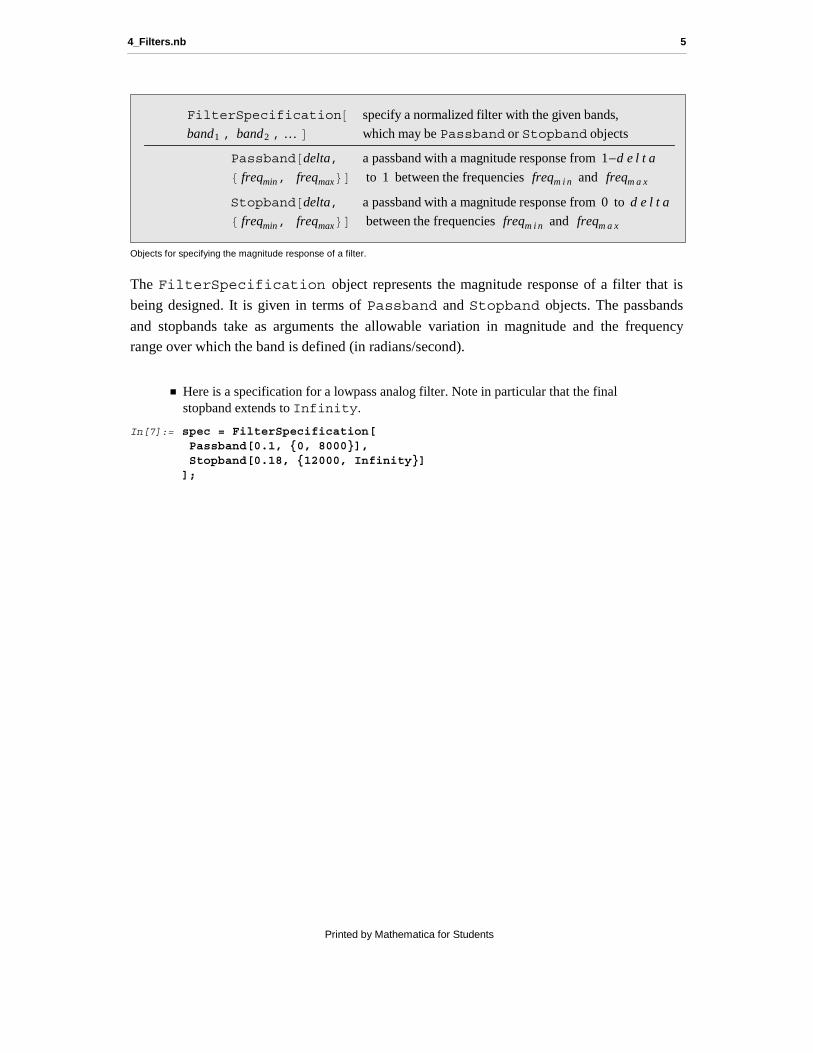
† Here is one way to visualize the specification. Note that the Infinity needed to be transformed to a finite value so that a nice graph could be generated.
In[8]:= graph = Show[Graphics[ {GrayLevel[0.8], Map[If[Head[#] === Stopband, Rectangle[{#[[2,1]], 0}, {#[[2,2]], #[[1]]} ], Rectangle[{#[[2,1]], 1 - #[[1]]}, {#[[2,2]], 1} ] ]&, List @@ spec/.Infinity -> 20000]}, Frame -> True, PlotRange -> All]]
0 5000 10000 15000 200000
0.2
0.4
0.6
0.8
1
Out[8]= Graphics
You can specify lowpass, highpass, bandpass, and bandstop filters with theFilterSpecification object. General multiband filters can be given in principle, but
the current design routines do not handle those cases.
Be aware that the FilterSpecification object has the attribute Orderless. This
means that Mathematica sorts the arguments in canonical (alphanumeric) order. They will notbe arranged by frequency range. Remember this particularly when writing programs based on
the FilterSpecification object.
6 4_Filters.nb
Printed by Mathematica for Students
† This bandpass specification demonstrates the automatic reordering of FilterSpecification arguments.
In[9]:= FilterSpecification[ Stopband[0.2, {0, 4000}], Passband[0.14, {6000, 8000}], Stopband[0.35, {9000, Infinity}]]
Out[9]= FilterSpecification@[email protected], 86000, 8000<D,[email protected], 80, 4000<D, [email protected], 89000, ∞<DD
The filter specification is passed to a design procedure to create a filter object. Currently, theonly analog design function is DesignAnalogFilter, which is used to create standard
analog filter types. The resulting analog filters may be used as prototypes for digital filterdesign.
DesignAnalogFilter@type, var, specD design a filter of the named type, with a particular
filter specification spec and the time variable var
Designing an analog filter.
DesignAnalogFilter enables automated design of a filter from an input filter
specification and a given filter type. If the filter paramaters are for a type of filter other thanlowpass, the specification will first be transformed to a lowpass type, then the resulting filter
will be inversely processed by transformation of the poles and zeros (seeAnalogFilterTransformation, below).
† Here is a lowpass elliptic filter designed with the specification we entered above. The result is a third-order filter.
In[10]:= filt = DesignAnalogFilter[ Elliptic, t, spec]
Out[10]= H1812.3 + 1.91466× 10⁻¹⁴ LAnalogFilter@8−4898.74 + 0. , −1543.22 − 8003.53 ,
−1543.22 + 8003.53 <, 813400.9 , −13400.9 <, tD
4_Filters.nb 7
Printed by Mathematica for Students
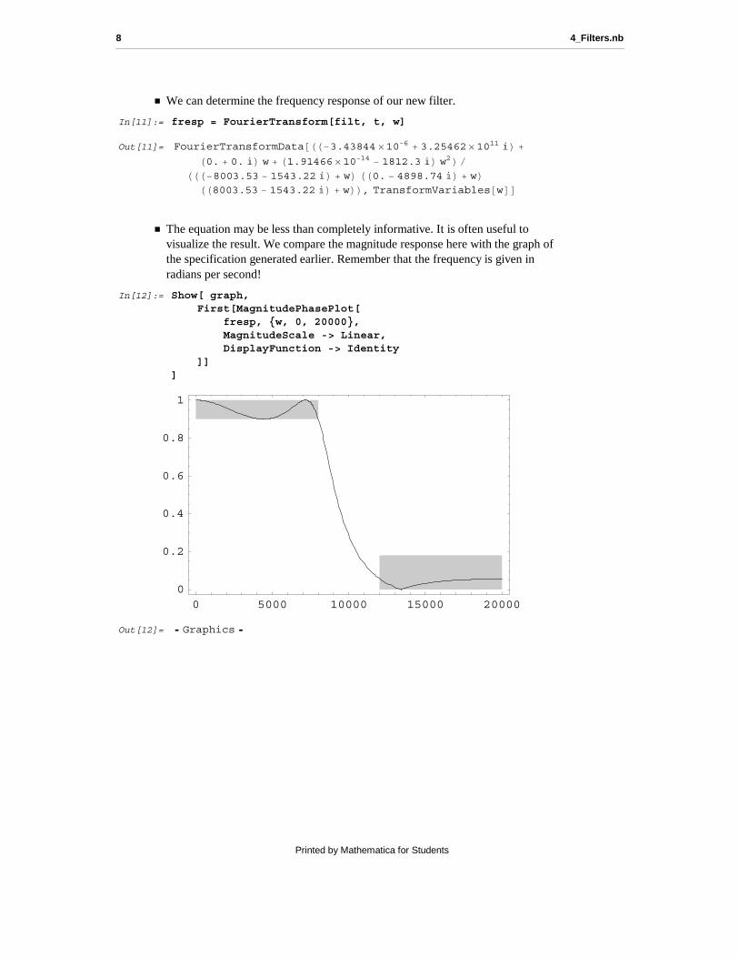
† We can determine the frequency response of our new filter.
In[11]:= fresp = FourierTransform[filt, t, w]
Out[11]= FourierTransformData@HH−3.43844 ×10⁻⁶ + 3.25462×10¹¹ L +H0. + 0. L w + H1.91466×10−14 − 1812.3 L w2LêHHH−8003.53 − 1543.22 L + wL HH0. − 4898.74 L + wLHH8003.53 − 1543.22 L + wLL, TransformVariables@wDD† The equation may be less than completely informative. It is often useful to
visualize the result. We compare the magnitude response here with the graph of the specification generated earlier. Remember that the frequency is given in radians per second!
In[12]:= Show[ graph, First[MagnitudePhasePlot[ fresp, {w, 0, 20000}, MagnitudeScale -> Linear, DisplayFunction -> Identity ]]]
0 5000 10000 15000 200000
0.2
0.4
0.6
0.8
1
Out[12]= Graphics
8 4_Filters.nb
Printed by Mathematica for Students
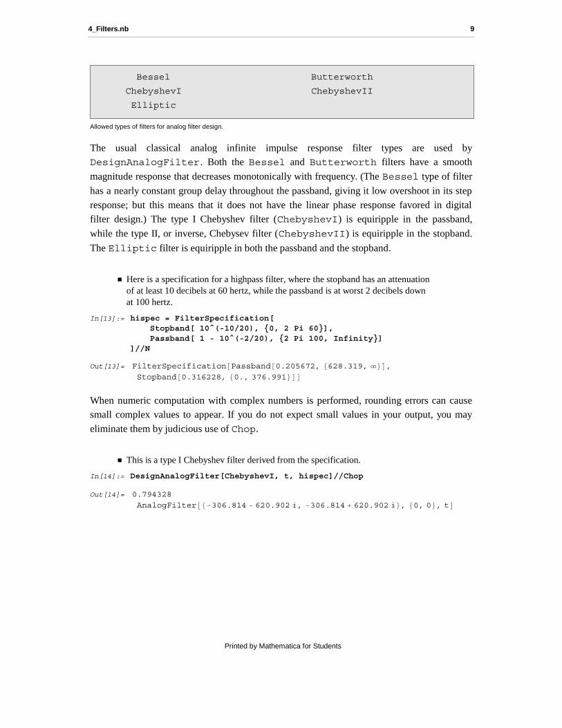
Bessel Butterworth
ChebyshevI ChebyshevII
Elliptic
Allowed types of filters for analog filter design.
The usual classical analog infinite impulse response filter types are used byDesignAnalogFilter. Both the Bessel and Butterworth filters have a smooth
magnitude response that decreases monotonically with frequency. (The Bessel type of filter
has a nearly constant group delay throughout the passband, giving it low overshoot in its step
response; but this means that it does not have the linear phase response favored in digitalfilter design.) The type I Chebyshev filter (ChebyshevI) is equiripple in the passband,
while the type II, or inverse, Chebysev filter (ChebyshevII) is equiripple in the stopband.
The Elliptic filter is equiripple in both the passband and the stopband.
† Here is a specification for a highpass filter, where the stopband has an attenuation of at least 10 decibels at 60 hertz, while the passband is at worst 2 decibels down at 100 hertz.
In[13]:= hispec = FilterSpecification[ Stopband[ 10^(-10/20), {0, 2 Pi 60}], Passband[ 1 - 10^(-2/20), {2 Pi 100, Infinity}]]//N
Out[13]= FilterSpecification@[email protected], 8628.319, ∞<D,[email protected], 80., 376.991<DD
When numeric computation with complex numbers is performed, rounding errors can causesmall complex values to appear. If you do not expect small values in your output, you may
eliminate them by judicious use of Chop.
† This is a type I Chebyshev filter derived from the specification.
In[14]:= DesignAnalogFilter[ChebyshevI, t, hispec]//Chop
Out[14]= 0.794328
AnalogFilter@8−306.814 − 620.902 , −306.814 + 620.902 <, 80, 0<, tD
4_Filters.nb 9
Printed by Mathematica for Students

† Here is the frequency response of the filter.
In[15]:= FourierTransform[%, t, w]//Chop
Out[15]= FourierTransformDataA 0.794328 w2
−479654. − 613.628 w + w2, TransformVariables@wDE
† We can check that the response has the desired characteristics. Here, we verify that the stopband attenuation is at least 10 decibels.
In[16]:= 20 Log[10, Abs[Normal[%]/.w -> 2 Pi 60]]//N
Out[16]= −11.1854
FilterOrder −> n generate a filter of order n, rather
than letting the order be computed automatically
Option to DesignAnalogFilter.
In some cases, the order of a filter that meets the given specification cannot be determinedautomatically by DesignAnalogFilter, or you may wish to design the filter with a
particular order. In these cases, you can explicitly specify an order for the filter by the option
FilterOrder. The order should be a positive integer. (The default value is the setting
Automatic, which tells DesignAnalogFilter to use the standard algorithms for
determining the minimum filter order which meets the specification.)
† Using the lowpass filter specification employed in the first example, we attempt to design a Bessel filter. The filter order could not be determined automatically, so a twelfth-order filter was used instead.
In[17]:= DesignAnalogFilter[Bessel, t, spec]
Bessel::order : Could not determine the order of the Bessel filter to
meet the specifications, so an order 12 will be used.
Out[17]= 2.18027× 1052 AnalogFilter@8−20885.4 − 2195.71 , −20885.4 + 2195.71 , −20237.2 − 6602.28 ,
−20237.2 + 6602.28 , −18891.7 − 11058.8 , −18891.7 + 11058.8 ,
−16729.2 − 15617.1 , −16729.2 + 15617.1 , −13486.9 − 20378. ,−13486.9 + 20378. , −8459.56 − 25619.7 , −8459.56 + 25619.7 <, 8<, tD
10 4_Filters.nb
Printed by Mathematica for Students
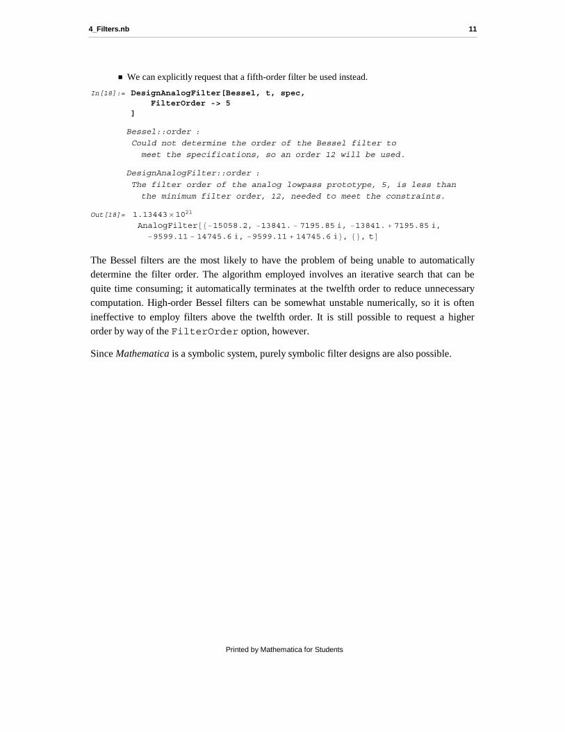
† We can explicitly request that a fifth-order filter be used instead.
In[18]:= DesignAnalogFilter[Bessel, t, spec, FilterOrder -> 5]
Bessel::order : Could not determine the order of the Bessel filter to
meet the specifications, so an order 12 will be used.
DesignAnalogFilter::order :
The filter order of the analog lowpass prototype, 5, is less than
the minimum filter order, 12, needed to meet the constraints.
Out[18]= 1.13443× 10²¹
AnalogFilter@8−15058.2, −13841. − 7195.85 , −13841. + 7195.85 ,
−9599.11 − 14745.6 , −9599.11 + 14745.6 <, 8<, tDThe Bessel filters are the most likely to have the problem of being unable to automaticallydetermine the filter order. The algorithm employed involves an iterative search that can bequite time consuming; it automatically terminates at the twelfth order to reduce unnecessarycomputation. High-order Bessel filters can be somewhat unstable numerically, so it is often
ineffective to employ filters above the twelfth order. It is still possible to request a higherorder by way of the FilterOrder option, however.
Since Mathematica is a symbolic system, purely symbolic filter designs are also possible.
4_Filters.nb 11
Printed by Mathematica for Students
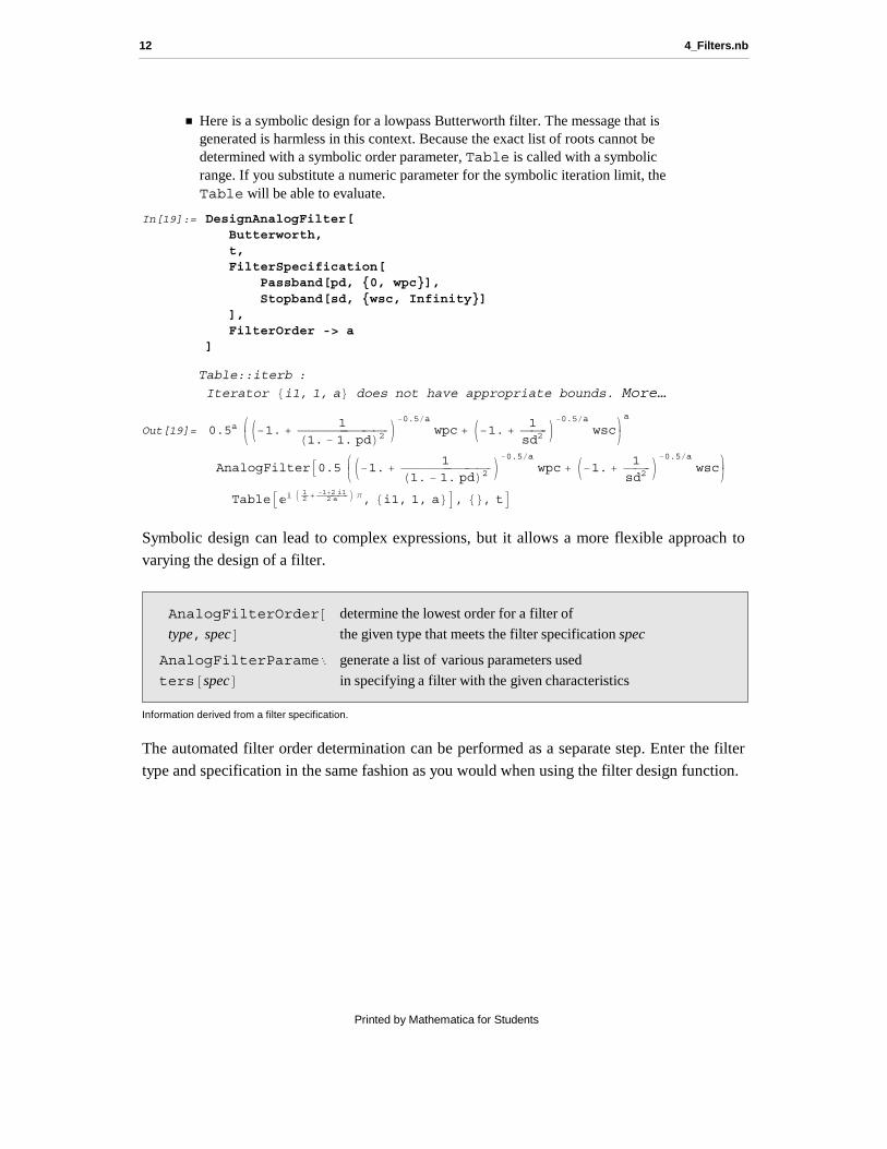
† Here is a symbolic design for a lowpass Butterworth filter. The message that is generated is harmless in this context. Because the exact list of roots cannot be determined with a symbolic order parameter, Table is called with a symbolic range. If you substitute a numeric parameter for the symbolic iteration limit, the Table will be able to evaluate.
In[19]:= DesignAnalogFilter[ Butterworth, t, FilterSpecification[ Passband[pd, {0, wpc}], Stopband[sd, {wsc, Infinity}] ], FilterOrder -> a]
Table::iterb :
Iterator 8i1, 1, a< does not have appropriate bounds. More…
Out[19]= 0.5a ikjjJ−1. +1H1. − 1. pdL2 N−0.5êa
wpc + J−1. +1sd2
N−0.5êawscy{zza
AnalogFilterA0.5 ikjjJ−1. +1H1. − 1. pdL2 N−0.5êa
wpc + J−1. +1sd2
N−0.5êawscy{zz
TableA I 12 + −1+2 i1
2 a M π, 8i1, 1, a<E, 8<, tESymbolic design can lead to complex expressions, but it allows a more flexible approach tovarying the design of a filter.
AnalogFilterOrder@type, specD determine the lowest order for a filter of
the given type that meets the filter specification spec
AnalogFilterParame
ters@specD generate a list of various parameters used
in specifying a filter with the given characteristics
Information derived from a filter specification.
The automated filter order determination can be performed as a separate step. Enter the filtertype and specification in the same fashion as you would when using the filter design function.
12 4_Filters.nb
Printed by Mathematica for Students
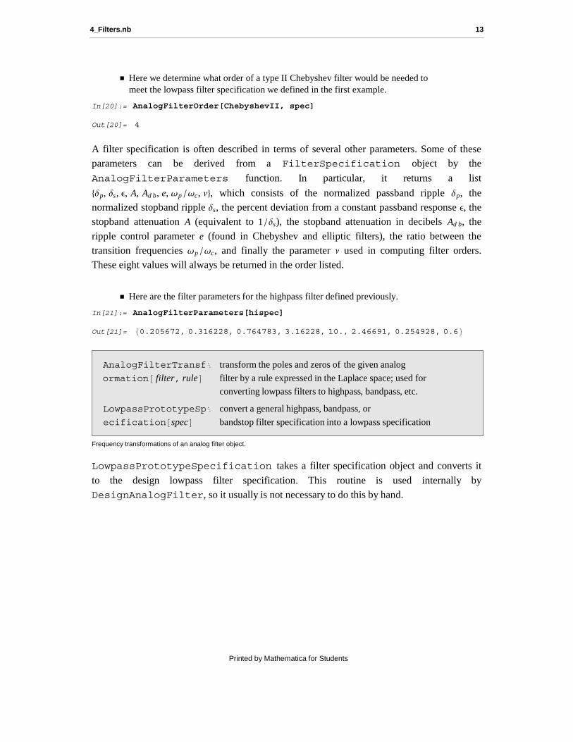
† Here we determine what order of a type II Chebyshev filter would be needed to meet the lowpass filter specification we defined in the first example.
In[20]:= AnalogFilterOrder[ChebyshevII, spec]
Out[20]= 4
A filter specification is often described in terms of several other parameters. Some of theseparameters can be derived from a FilterSpecification object by the
AnalogFilterParameters function. In particular, it returns a list8dp, ds, e, A, Ad b, e, wp ê wc, n<, which consists of the normalized passband ripple dp, thenormalized stopband ripple ds, the percent deviation from a constant passband response e, thestopband attenuation A (equivalent to 1 ê ds), the stopband attenuation in decibels Ad b, the
ripple control parameter e (found in Chebyshev and elliptic filters), the ratio between thetransition frequencies wp ê wc, and finally the parameter n used in computing filter orders.These eight values will always be returned in the order listed.
† Here are the filter parameters for the highpass filter defined previously.
In[21]:= AnalogFilterParameters[hispec]
Out[21]= 80.205672, 0.316228, 0.764783, 3.16228, 10., 2.46691, 0.254928, 0.6<AnalogFilterTransf
ormation@ filter, ruleD transform the poles and zeros of the given analog
filter by a rule expressed in the Laplace space; used for
converting lowpass filters to highpass, bandpass, etc.
LowpassPrototypeSp
ecification@specD convert a general highpass, bandpass, or
bandstop filter specification into a lowpass specification
Frequency transformations of an analog filter object.
LowpassPrototypeSpecification takes a filter specification object and converts it
to the design lowpass filter specification. This routine is used internally byDesignAnalogFilter, so it usually is not necessary to do this by hand.
4_Filters.nb 13
Printed by Mathematica for Students

† Here is the lowpass specification used in the design of the highpass filter defined earlier.
In[22]:= LowpassPrototypeSpecification[hispec]
Out[22]= FilterSpecification@[email protected], 80., 0.00159155<D,[email protected], 80.00265258, ∞<DD
The AnalogFilterTransformation function performs arbitrary mappings of the
poles and zeros of a filter object. These mappings are used to convert a lowpass filter to the
requested highpass, bandpass, bandstop, etc. filter by DesignAnalogFilter. However,
an arbitrary mapping can be employed. The first argument is the filter, while the second isgiven in the form of a transformation rule. The rule should be a mapping of the state-space
variable to some other expression (any symbol can be used for the state-space variable).
s −> a s lowpass to lowpass
s −> aês lowpass to highpass
s −> a Hs^2 + s0 L lowpass to bandpass
s −> a sêHb s^2 + s0 L lowpass to bandstop
Some common mappings for use with AnalogFilterTransformation.
The parameters involved in the transformation take on different meanings depending on thedesign procedure involved.
† Here is a normalized third-order lowpass Butterworth filter. Note that the poles are the roots of the third-order Butterworth polynomial. We will use this filter to design a highpass filter.
In[23]:= filt = AnalogFilter[ GetRootList[(s + 1)(s^2 + s + 1), s], {}, t]
Out[23]= AnalogFilter@8−1., −0.5 − 0.866025 , −0.5 + 0.866025 <, 8<, tD
14 4_Filters.nb
Printed by Mathematica for Students
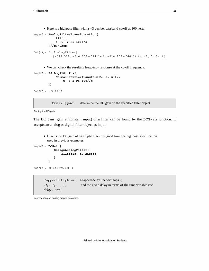
† Here is a highpass filter with a -3 decibel passband cutoff at 100 hertz.
In[24]:= AnalogFilterTransformation[ filt, s -> (2 Pi 100)/s]//N//Chop
Out[24]= 1. AnalogFilter@8−628.319, −314.159 + 544.14 , −314.159 − 544.14 <, 80, 0, 0<, tD† We can check the resulting frequency response at the cutoff frequency.
In[25]:= 20 Log[10, Abs[ Normal[FourierTransform[%, t, w]]/. w -> 2 Pi 100//N]]
Out[25]= −3.0103
DCGain@ filterD determine the DC gain of the specified filter object
Finding the DC gain.
The DC gain (gain at constant input) of a filter can be found by the DCGain function. It
accepts an analog or digital filter object as input.
† Here is the DC gain of an elliptic filter designed from the highpass specification used in previous examples.
In[26]:= DCGain[ DesignAnalogFilter[ Elliptic, t, hispec ]]
Out[26]= 0.143775 + 0.
TappedDelayLine@8t1, t2, …<,delay, varD a tapped delay line with taps ti
and the given delay in terms of the time variable var
Representing an analog tapped delay line.
4_Filters.nb 15
Printed by Mathematica for Students
The closest thing to a finite impulse response (FIR) filter in the analog domain is the tappeddelay line. Its syntax is similar to the AnalogFilter object. In this case, the first argument
is the list of tap values and the second argument is the delay between the taps.
† Here is a tapped delay line.
In[27]:= dline = TappedDelayLine[ {1, -0.2, 0.3, -0.4}, 0.5, t];
† The impulse response can be found in the same fashion as that used for an analog filter object.
In[28]:= EvaluateOperators[ dline[DiracDelta[t]]]
Out[28]= −0.4 DiracDelta@−1.5 + tD + 0.3 DiracDelta@−1. + tD −
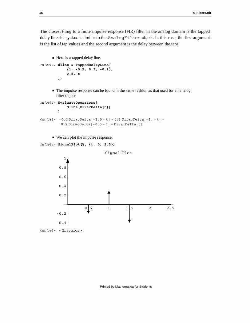
0.2 DiracDelta@−0.5 + tD + DiracDelta@tD† We can plot the impulse response.
In[29]:= SignalPlot[%, {t, 0, 2.5}]
0.5 1 1.5 2 2.5
-0.4
-0.2
0.2
0.4
0.6
0.8
1
Signal Plot
Out[29]= Graphics
16 4_Filters.nb
Printed by Mathematica for Students
à 4.2 Digital Filter Design
Signals and Systems naturally provides representations for working with filters in the
discrete-time domain. In particular, general pole-zero filters (usually infinite impulse response(IIR)) can be manipulated by way of DigitalFilter, while all-zero finite impulse
response (FIR) filters are represented with DigitalFIRFilter.
DigitalFilter@8p1, p2, …<,8z1, z2, …<, varD a digital Hdiscrete-timeL IIR filter with poles pi and zeros zi in the specified time variable
Representing a digital IIR filter.
The DigitalFilter object takes a list of poles and a list of zeros of the transfer function
to specify a particular digital filter. This notation is particularly useful for design techniquesbased on pole-zero placement. The DigitalFilter object is a Signals and Systems
operator. Like AnalogFilter, it is used in operator form to determine the output of a
signal passing through the filter. The filter object can be passed directly to transformfunctions to find out about various filter characteristics, such as the transfer function or thefrequency response.
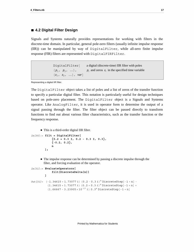
† This is a third-order digital IIR filter.
In[30]:= filt = DigitalFilter[ {0.2 + 0.3 I, 0.2 - 0.3 I, 0.3}, {-0.2, 0.2}, n];
† The impulse response can be determined by passing a discrete impulse through the filter, and forcing evaluation of the operator.
In[31]:= EvaluateOperators[ filt[DiscreteDelta[n]]]
Out[31]= H−1.34615 + 1.73077 L H0.2 − 0.3 Ln DiscreteStep@−1 + nD −H1.34615 + 1.73077 L H0.2 + 0.3 Ln DiscreteStep@−1 + nD +H1.66667 − 3.23905× 10⁻¹⁷ L 0.3n DiscreteStep@−1 + nD
4_Filters.nb 17
Printed by Mathematica for Students
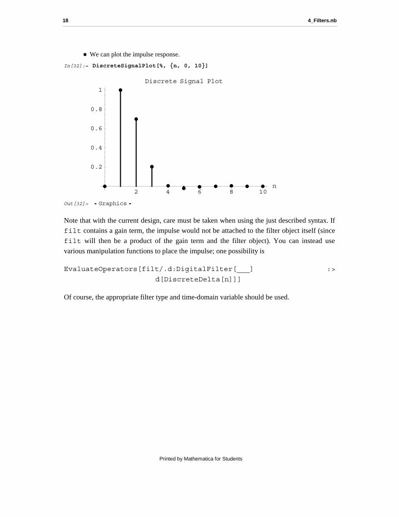
† We can plot the impulse response.
In[32]:= DiscreteSignalPlot[%, {n, 0, 10}]
2 4 6 8 10n
0.2
0.4
0.6
0.8
1
Discrete Signal Plot
Out[32]= Graphics
Note that with the current design, care must be taken when using the just described syntax. If
filt contains a gain term, the impulse would not be attached to the filter object itself (since
filt will then be a product of the gain term and the filter object). You can instead use
various manipulation functions to place the impulse; one possibility is
EvaluateOperators[filt/.d:DigitalFilter[___] :>
d[DiscreteDelta[n]]]
Of course, the appropriate filter type and time-domain variable should be used.
18 4_Filters.nb
Printed by Mathematica for Students
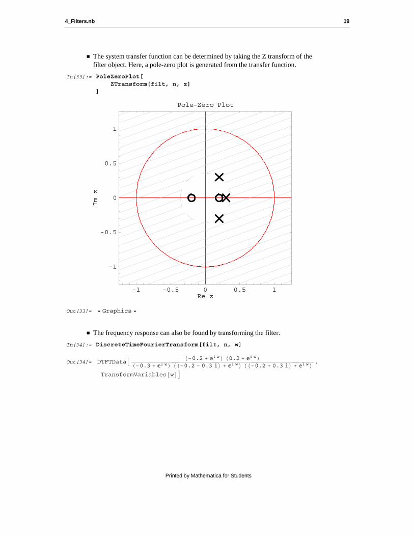
† The system transfer function can be determined by taking the Z transform of the filter object. Here, a pole-zero plot is generated from the transfer function.
In[33]:= PoleZeroPlot[ ZTransform[filt, n, z]]
-1 -0.5 0 0.5 1Re z
-1
-0.5
0
0.5
1
mI
z
Pole−Zero Plot
Out[33]= Graphics
† The frequency response can also be found by transforming the filter.
In[34]:= DiscreteTimeFourierTransform[filt, n, w]
Out[34]= DTFTDataA H−0.2 + wL H0.2 + wLH−0.3 + wL HH−0.2 − 0.3 L + wL HH−0.2 + 0.3 L + wL ,
TransformVariables@wDE
4_Filters.nb 19
Printed by Mathematica for Students
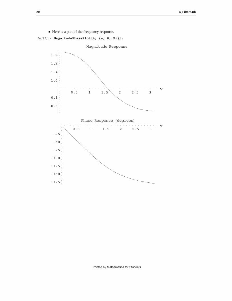
† Here is a plot of the frequency response.
In[35]:= MagnitudePhasePlot[%, {w, 0, Pi}];
0.5 1 1.5 2 2.5 3w
0.6
0.8
1.2
1.4
1.6
1.8
Magnitude Response
0.5 1 1.5 2 2.5 3w
-175
-150
-125
-100
-75
-50
-25
Phase Response HdegreesL
20 4_Filters.nb
Printed by Mathematica for Students
ImpulseInvariance@ filter, Td , t, nD convert the given analog filter in t into
a digital filter in n by the method of impulse
invariance with design sampling period Td
BilinearTransformation@filter, Td , t, nD convert the given analog filter
in t into a digital filter in n by the bilinear
transform with design sampling period Td
Methods for converting an analog prototype filter into a digital filter.
Classical design techniques for digital IIR filters involve prototyping the filter with an analogdesign, then transforming it to a digital filter. The functions ImpulseInvariance and
BilinearTransformation perform the conversion of analog filters to digital filters.
In signal processing applications, design by impulse invariance usually works directly from a
digital specification. In Signals and Systems, however, the design is implemented as atransformation of an analog filter object. Hence, the design sampling period Td must be inputto the transformation routine. (Note that Td is not necessarily the frequency at which the filteroperates.) When an analog filter is being designed specifically for a digital application, it is
useful to specify the corner frequencies in the normalized digital frequency space (between 0and p). If this is done, you can set Td to 1 without any problems.
Be aware that this procedure is only appropriate for bandlimited prototypes. Highpass andbandstop filters, for instance, will show severe aliasing when designed by impulse invariance.
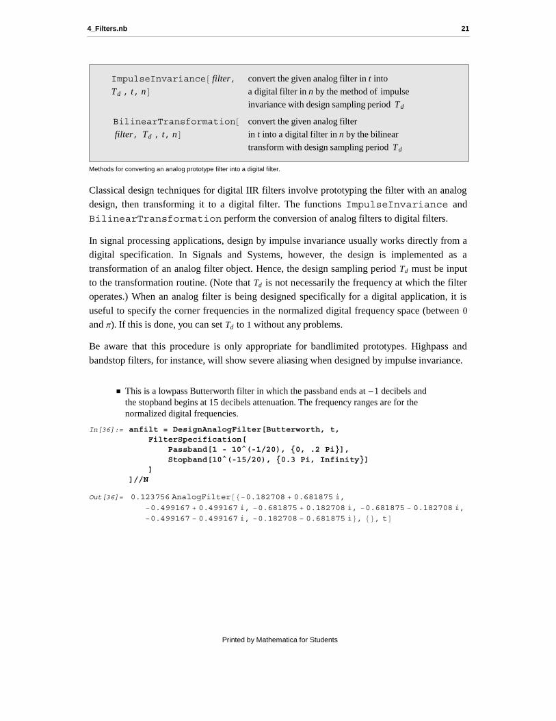
† This is a lowpass Butterworth filter in which the passband ends at -1 decibels and the stopband begins at 15 decibels attenuation. The frequency ranges are for the normalized digital frequencies.
In[36]:= anfilt = DesignAnalogFilter[Butterworth, t, FilterSpecification[ Passband[1 - 10^(-1/20), {0, .2 Pi}], Stopband[10^(-15/20), {0.3 Pi, Infinity}] ]]//N
Out[36]= 0.123756 AnalogFilter@8−0.182708 + 0.681875 ,
−0.499167 + 0.499167 , −0.681875 + 0.182708 , −0.681875 − 0.182708 ,−0.499167 − 0.499167 , −0.182708 − 0.681875 <, 8<, tD
4_Filters.nb 21
Printed by Mathematica for Students
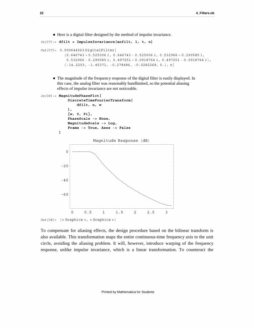
† Here is a digital filter designed by the method of impulse invariance.
In[37]:= dfilt = ImpulseInvariance[anfilt, 1, t, n]
Out[37]= 0.000644563 [email protected] + 0.525006 , 0.646743 − 0.525006 , 0.532966 + 0.290585 ,0.532966 − 0.290585 , 0.497251 + 0.0918764 , 0.497251 − 0.0918764 <,8−14.2203, −1.45371, −0.278486, −0.0282268, 0.<, nD
† The magnitude of the frequency response of the digital filter is easily displayed. In this case, the analog filter was reasonably bandlimited, so the potential aliasing effects of impulse invariance are not noticeable.
In[38]:= MagnitudePhasePlot[ DiscreteTimeFourierTransform[ dfilt, n, w ], {w, 0, Pi}, PhaseScale -> None, MagnitudeScale -> Log, Frame -> True, Axes -> False]
0 0.5 1 1.5 2 2.5 3
-60
-40
-20
0
Magnitude Response HdBL
Out[38]= 8 Graphics , Graphics <To compensate for aliasing effects, the design procedure based on the bilinear transform isalso available. This transformation maps the entire continuous-time frequency axis to the unit
circle, avoiding the aliasing problem. It will, however, introduce warping of the frequencyresponse, unlike impulse invariance, which is a linear transformation. To counteract the
22 4_Filters.nb
Printed by Mathematica for Students
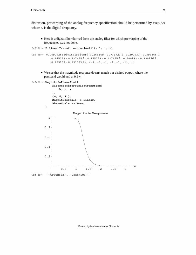
distortion, prewarping of the analog frequency specification should be performed by tanHw ê2Lwhere w is the digital frequency.
† Here is a digital filter derived from the analog filter for which prewarping of the frequencies was not done.
In[39]:= BilinearTransformation[anfilt, 1, t, n]
Out[39]= 0.00929256 [email protected] + 0.731723 , 0.200933 + 0.399866 ,0.175279 + 0.127675 , 0.175279 − 0.127675 , 0.200933 − 0.399866 ,
0.269169 − 0.731723 <, 8−1, −1, −1, −1, −1, −1<, nD† We see that the magnitude response doesn't match our desired output, where the
passband would end at 0.2 p.
In[40]:= MagnitudePhasePlot[ DiscreteTimeFourierTransform[ %, n, w ], {w, 0, Pi}, MagnitudeScale -> Linear, PhaseScale -> None]
0.5 1 1.5 2 2.5 3w
0.2
0.4
0.6
0.8
1
Magnitude Response
Out[40]= 8 Graphics , Graphics <
4_Filters.nb 23
Printed by Mathematica for Students

† Here, we redesign the analog filter with prewarped frequency bands.
In[41]:= DesignAnalogFilter[Butterworth, t, FilterSpecification[ Passband[1 - 10^(-1/20), {0, Tan[.2 Pi/2]}], Stopband[10^(-15/20), {Tan[0.3 Pi/2], Infinity}] ]]//N
Out[41]= 0.00270961 AnalogFilter@8−0.0966379 + 0.360657 ,
−0.26402 + 0.26402 , −0.360657 + 0.0966379 , −0.360657 − 0.0966379 ,
−0.26402 − 0.26402 , −0.0966379 − 0.360657 <, 8<, tD† This is the new digital filter derived from the redesigned analog filter.
In[42]:= bilinfilt = BilinearTransformation[%, 1, t, n]
Out[42]= 0.000655303 [email protected] + 0.541248 , 0.516109 + 0.316674 ,0.4625 + 0.103871 , 0.4625 − 0.103871 , 0.516109 − 0.316674 ,
0.645753 − 0.541248 <, 8−1, −1, −1, −1, −1, −1<, nD
24 4_Filters.nb
Printed by Mathematica for Students
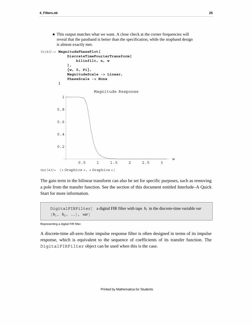
† This output matches what we want. A close check at the corner frequencies will reveal that the passband is better than the specification, while the stopband design is almost exactly met.
In[43]:= MagnitudePhasePlot[ DiscreteTimeFourierTransform[ bilinfilt, n, w ], {w, 0, Pi}, MagnitudeScale -> Linear, PhaseScale -> None]
0.5 1 1.5 2 2.5 3w
0.2
0.4
0.6
0.8
1
Magnitude Response
Out[43]= 8 Graphics , Graphics <The gain term in the bilinear transform can also be set for specific purposes, such as removing
a pole from the transfer function. See the section of this document entitled Interlude–A QuickStart for more information.
DigitalFIRFilter@8h1, h2, …<, varD a digital FIR filter with taps hi in the discrete-time variable var
Representing a digital FIR filter.
A discrete-time all-zero finite impulse response filter is often designed in terms of its impulseresponse, which is equivalent to the sequence of coefficients of its transfer function. TheDigitalFIRFilter object can be used when this is the case.
4_Filters.nb 25
Printed by Mathematica for Students
Perhaps the simplest technique for designing an FIR filter is to sample the ideal frequencyresponse. The most common expression of the ideal response is for it to be 1 in the passbandand 0 elsewhere. Remembering the symmetry of the discrete-time Fourier transform, we canwrite the ideal response as a sum of pulses. The samples can be multiplied by an additional
exponential term to generate a linear phase response.
† This small function will generate the ideal response for a linear phase FIR lowpass filter, with the normalized cutoff frequency given as the first argument in radians per second, and the filter length given as the second argument.
In[44]:= idealResponse[cutoff_, length_] := Drop[Table[ Exp[-I t (length - 1)/2] (ContinuousPulse[2 cutoff, t + cutoff] + ContinuousPulse[2 cutoff, t - 2 Pi + cutoff]), {t, 0, 2 Pi, 2 Pi/length}], -1]//N
We can conveniently use the special vector input form of theInverseDiscreteFourierTransform function.
† Here is the truncated impulse response of the ideal filter. This is equivalent to the coefficients of the filter's transfer function.
In[45]:= impresp = InverseDiscreteFourierTransform[ idealResponse[0.4 Pi, 17]]//Chop
Out[45]= 8−0.0471433, 0.0220929, 0.0654323, 0.0135446, −0.0781609, −0.0752788,0.0857227, 0.307908, 0.411765, 0.307908, 0.0857227, −0.0752788,
−0.0781609, 0.0135446, 0.0654323, 0.0220929, −0.0471433<† An FIR filter object is easily constructed from the impulse response given as a
vector.
In[46]:= dfilt = DigitalFIRFilter[impresp, n];
26 4_Filters.nb
Printed by Mathematica for Students
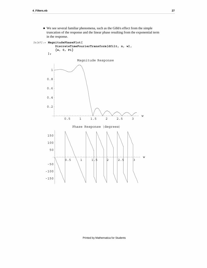
† We see several familiar phenomena, such as the Gibb's effect from the simple truncation of the response and the linear phase resulting from the exponential term in the response.
In[47]:= MagnitudePhasePlot[ DiscreteTimeFourierTransform[dfilt, n, w], {w, 0, Pi}];
0.5 1 1.5 2 2.5 3w
0.2
0.4
0.6
0.8
1
Magnitude Response
0.5 1 1.5 2 2.5 3w
-150
-100
-50
50
100
150
Phase Response HdegreesL
4_Filters.nb 27
Printed by Mathematica for Students
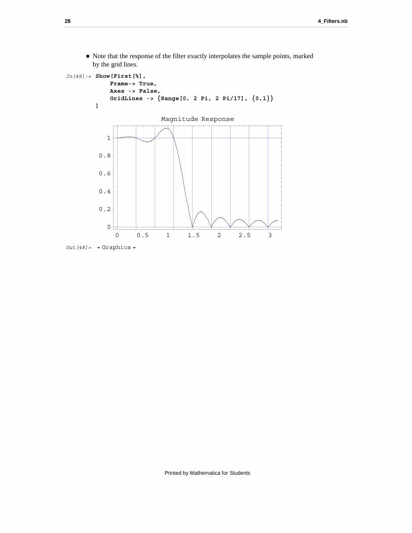
† Note that the response of the filter exactly interpolates the sample points, marked by the grid lines.
In[48]:= Show[First[%], Frame-> True, Axes -> False, GridLines -> {Range[0, 2 Pi, 2 Pi/17], {0,1}}]
0 0.5 1 1.5 2 2.5 30
0.2
0.4
0.6
0.8
1
Magnitude Response
Out[48]= Graphics
28 4_Filters.nb
Printed by Mathematica for Students
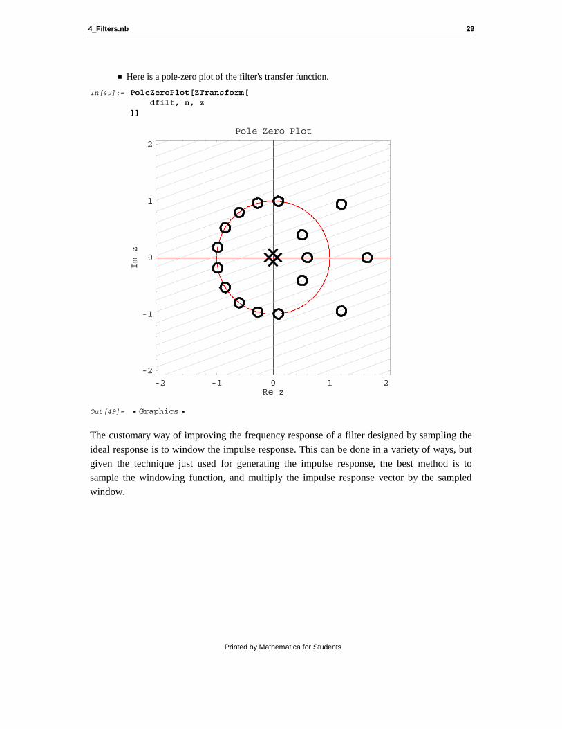
† Here is a pole-zero plot of the filter's transfer function.
In[49]:= PoleZeroPlot[ZTransform[ dfilt, n, z]]
-2 -1 0 1 2Re z
-2
-1
0
1
2mI
zPole−Zero Plot
Out[49]= Graphics
The customary way of improving the frequency response of a filter designed by sampling the
ideal response is to window the impulse response. This can be done in a variety of ways, butgiven the technique just used for generating the impulse response, the best method is tosample the windowing function, and multiply the impulse response vector by the sampledwindow.
4_Filters.nb 29
Printed by Mathematica for Students

† This samples a discrete Hamming window.
In[50]:= window = N[Table[ DiscreteWindow[Hamming, 17, n], {n, 0, 16}]];
† The filter object is created by multiplying the window vector and the impulse response computed above.
In[51]:= dfilt2 = DigitalFIRFilter[impresp window, n];
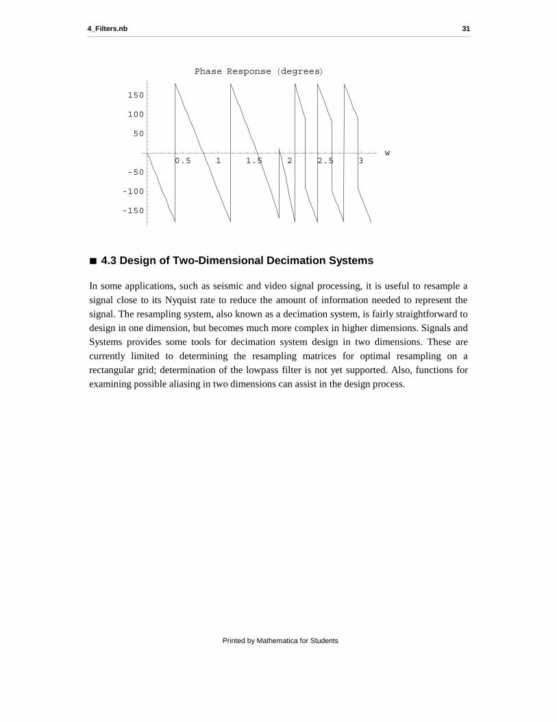
† Here is the frequency response of the windowed filter.
In[52]:= MagnitudePhasePlot[ DiscreteTimeFourierTransform[dfilt2, n, w], {w, 0, Pi}];
0.5 1 1.5 2 2.5 3w
0.2
0.4
0.6
0.8
1Magnitude Response
30 4_Filters.nb
Printed by Mathematica for Students
0.5 1 1.5 2 2.5 3w
-150
-100
-50
50
100
150
Phase Response HdegreesL
à 4.3 Design of Two-Dimensional Decimation Systems
In some applications, such as seismic and video signal processing, it is useful to resample a
signal close to its Nyquist rate to reduce the amount of information needed to represent thesignal. The resampling system, also known as a decimation system, is fairly straightforward todesign in one dimension, but becomes much more complex in higher dimensions. Signals andSystems provides some tools for decimation system design in two dimensions. These are
currently limited to determining the resampling matrices for optimal resampling on arectangular grid; determination of the lowpass filter is not yet supported. Also, functions forexamining possible aliasing in two dimensions can assist in the design process.
4_Filters.nb 31
Printed by Mathematica for Students
DesignDecimationSy
stem2D@polygonD determine the decimation system, specified as a shift
vector, an upsampling matrix, and a downsampling matrix,
that optimally samples the passband specified by polygon
DesignDecimationSy
stem2D@polygon, 8n1, n2<D determine the decimation system, returned as a cascade of
operators in the variables n1 , n2 instead of a list of matrices
DownsamplingAliasi
ng@matrix, polygonsD determine the possible aliasing of
passbands specified by a polygon or list of polygons
when downsampling by matrix is performed
Functions for assisting in the design of two-dimensional decimation systems.
A decimation system is defined as a cascade of a phase shifter (which centers the passbandabout the origin), an upsampler, a lowpass filter, and a downsampler. The passband isspecified as a two-dimensional polygon in the frequency domain, normalized to thefundamental frequency tile, using the syntax of the Mathematica Polygon graphics
primitive. The decimator design will be based on circumscribing the convex hull of thepassband with a minimal parallelogram. The parallelogram will be aligned on the grid pointsof the fundamental frequency tile, determined by the GridPoints option. A set of
resampling matrices and the shift vector that can be used to map the parallelogram to the
fundamental frequency tile will be returned. Alternately, a cascade of Signals and Systemsoperators that perform this computation can be generated.
† Here is a polygon specifying a particular passband.
In[53]:= poly = Polygon[{{-1.95, -1.94}, {-1.01, -1.64}, {-0.29, -1.05}, {0.29, -0.47}, {0.99, 0.47}, {1.54, 1.16}, {1.92, 2.07}, {1.20, 1.97}, {0.57, 1.66}, {0.07, 1.16}, {-0.51, 0.66}, {-1.17, -0.06}, {-1.70, -0.93}}];
32 4_Filters.nb
Printed by Mathematica for Students
† Here is the decimation system determined to best sample this passband given a rectangular sampling grid and the current setting for the GridPoints option.
In[54]:= DesignDecimationSystem2D[poly]
Out[54]= 99−39 π725
,157 π5800
=, 88−9009, 1001<, 813750894, −1527877<<,888736, 34925<, 8−13334200, −53307800<<=† This is the system expressed as operators.
In[55]:= DesignDecimationSystem2D[ poly, {n1, n2}]
Out[55]=ikjjjjDownsample8736 34925
−13334200 −53307800
»» n1
n2
y{zzzzADiscreteConvolution8n1,n2<Afilter1@n1, n2D,ikjjjjUpsample−9009 1001
13750894 −1527877
»» n1
n2
y{zzzzA H− 39 n1 π725 + 157 n2 π
5800 L x1@n1, n2DEEEGridPoints −> m,
GridPoints −> 8m1, m2< specify the divisions of the fundamental frequency
tile to be used for the baseband paralellogram
Justification −> All report information about
the decimation system being determined
Options for DesignDecimationSystem2D.
A good deal of useful information can be determined during this design process, such as thetheoretical best and the actual achieved compression ratios, assuming an initial rectangularsampling grid. Visualization of the design process can also be performed. This information
can be generated in the form of a report by use of the Justification option.
† Here is a report of the design procedure.
In[56]:= DesignDecimationSystem2D[ poly, Justification -> All]
The theoretical upper limit on the compression ratio,
computed as the ratio of 4 Pi^2 over the area of the
4_Filters.nb 33
Printed by Mathematica for Students
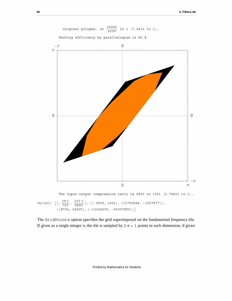
original polygon, is160002209
to 1 H7.2431 to 1L.Packing efficiency by parallelogram is 80.%.
0 π
0
π−π 0
−π
0
The input−output compression ratio is 5800 to 1001 H5.79421 to 1L.Out[56]= 99−
39 π725
,157 π5800
=, 88−9009, 1001<, 813750894, −1527877<<,888736, 34925<, 8−13334200, −53307800<<=The GridPoints option specifies the grid superimposed on the fundamental frequency tile.
If given as a single integer n, the tile is sampled by 2 n + 1 points in each dimension; if given
34 4_Filters.nb
Printed by Mathematica for Students
as a pair of integers n1 and n2 the grid has 2 n1 + 1 points on the horizontal axis and 2 n2 + 1
points on the vertical axis.
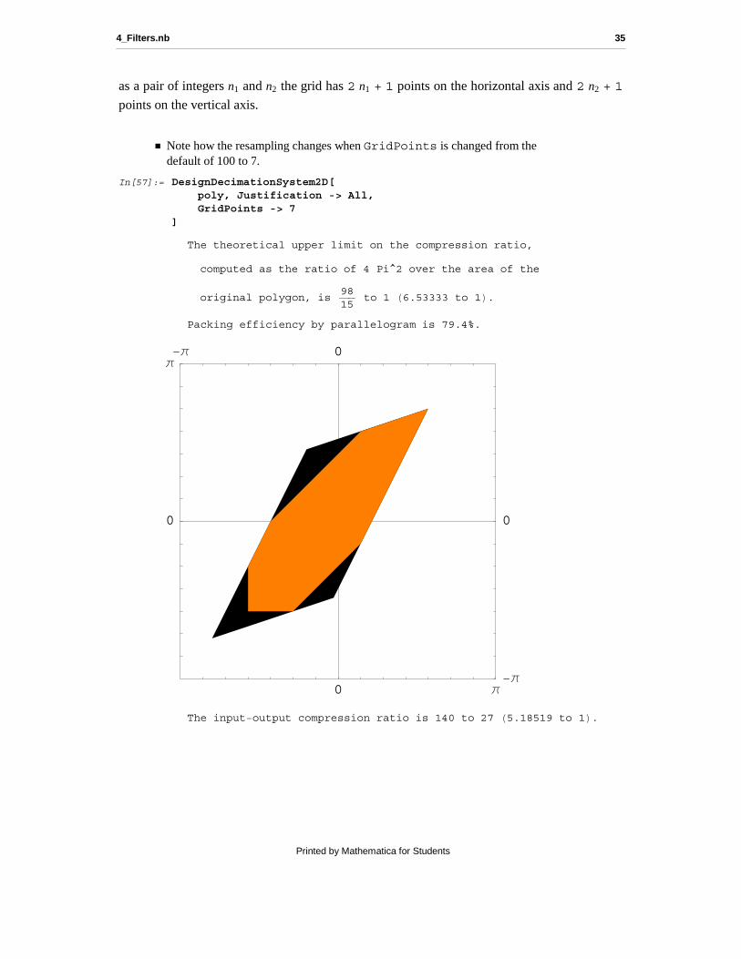
† Note how the resampling changes when GridPoints is changed from the default of 100 to 7.
In[57]:= DesignDecimationSystem2D[ poly, Justification -> All, GridPoints -> 7]
The theoretical upper limit on the compression ratio,
computed as the ratio of 4 Pi^2 over the area of the
original polygon, is9815
to 1 H6.53333 to 1L.Packing efficiency by parallelogram is 79.4%.
0 π
0
π−π 0
−π
0
The input−output compression ratio is 140 to 27 H5.18519 to 1L.
4_Filters.nb 35
Printed by Mathematica for Students
Out[57]= 99−4 π35
, −π70
=, 889, 0<, 8114, 3<<, 886, 28<, 870, 350<<=The DownsamplingAliasing function analyzes possible aliasing in a downsampling
operation. Downsampling in two dimensions produces images of the original baseband in thefundamental frequency tile. If these images overlap, aliasing occurs. The
DownsamplingAliasing function accepts the downsampling matrix as the first
argument, and the baseband polygon (or list of polygons) as the second argument. It returns alist of the image bands produced in the downsampling process. With the default option ofJustification -> All an informative report, including visualization of the possible
aliasing, is generated. You can also supply options controlling the graphics of thefundamental frequency tile.
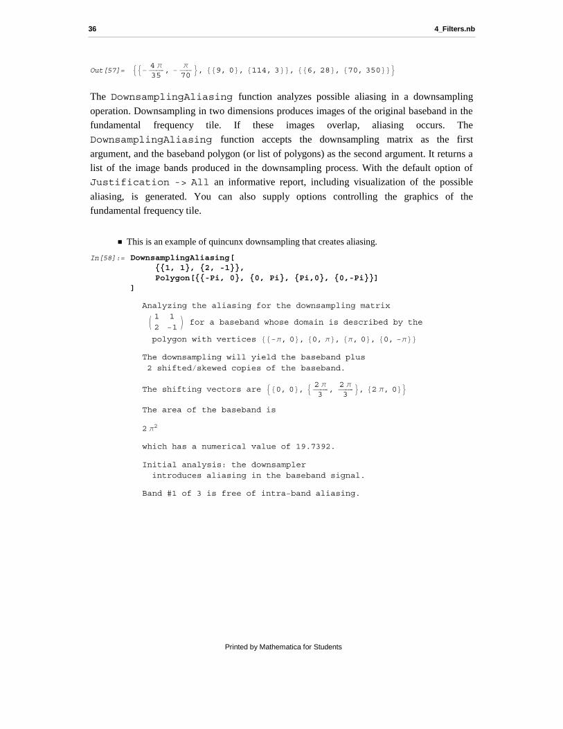
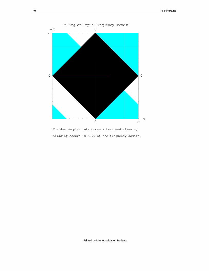
† This is an example of quincunx downsampling that creates aliasing.
In[58]:= DownsamplingAliasing[ {{1, 1}, {2, -1}}, Polygon[{{-Pi, 0}, {0, Pi}, {Pi,0}, {0,-Pi}}]]
Analyzing the aliasing for the downsampling matrixJ 1 1
2 −1N for a baseband whose domain is described by the
polygon with vertices 88−π, 0<, 80, π<, 8π, 0<, 80, −π<<The downsampling will yield the baseband plus
2 shiftedêskewed copies of the baseband.
The shifting vectors are 980, 0<, 9 2 π3
,2 π3
=, 82 π, 0<=The area of the baseband is
2 π2
which has a numerical value of 19.7392.
Initial analysis: the downsamplerintroduces aliasing in the baseband signal.
Band #1 of 3 is free of intra−band aliasing.
36 4_Filters.nb
Printed by Mathematica for Students
0 π
0
π−π 0
−π
0
Band #1 of 3
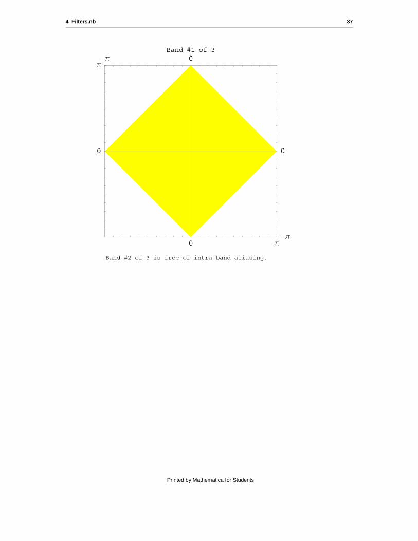
Band #2 of 3 is free of intra−band aliasing.
4_Filters.nb 37
Printed by Mathematica for Students
0 π
0
π−π 0
−π
0
Band #2 of 3
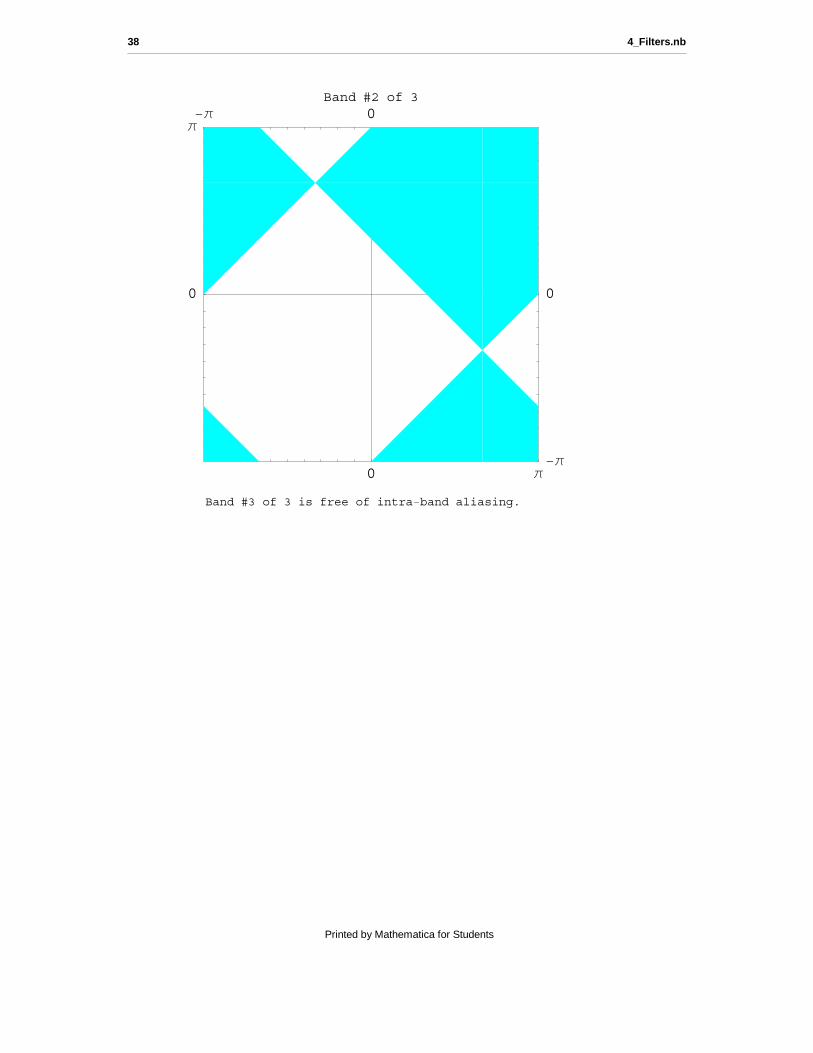
Band #3 of 3 is free of intra−band aliasing.
38 4_Filters.nb
Printed by Mathematica for Students
0 π
0
π−π 0
−π
0
Band #3 of 3
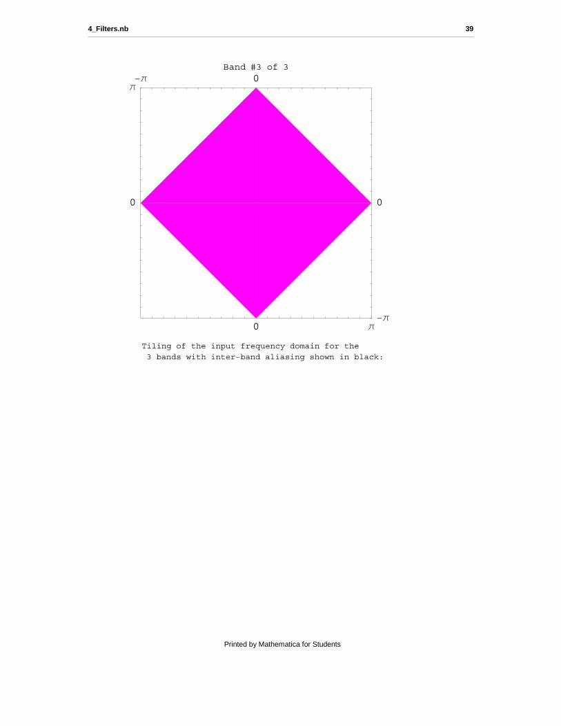
Tiling of the input frequency domain for the
3 bands with inter−band aliasing shown in black:
4_Filters.nb 39
Printed by Mathematica for Students
0 π
0
π−π 0
−π
0
Tiling of Input Frequency Domain
The downsampler introduces inter−band aliasing.
Aliasing occurs in 50.% of the frequency domain.
40 4_Filters.nb
Printed by Mathematica for Students
Out[58]= 88Polygon@88−3.14159, 0<, 80, 3.14159<, 80, 0<<D,Polygon@880, 3.14159<, 83.14159, 0<, 80, 0<<D,[email protected], 0<, 80, −3.14159<, 80, 0<<D,Polygon@880, −3.14159<, 8−3.14159, 0<, 80, 0<<D<,8Polygon@88−1.0472, 2.0944<, 80, 3.14159<,82.0944, 3.14159<, 82.0944, 2.0944<, 8−1.0472, 2.0944<<D,Polygon@880, −3.14159<, 82.0944, −1.0472<, 82.0944, −3.14159<<D,[email protected], 3.14159<, 83.14159, 2.0944<,82.0944, 2.0944<, 82.0944, 3.14159<<D,[email protected], −1.0472<, 83.14159, −2.0944<,83.14159, −3.14159<, 82.0944, −3.14159<, 82.0944, −1.0472<<D,Polygon@88−2.0944, 3.14159<, 8−1.0472, 2.0944<,8−3.14159, 2.0944<, 8−3.14159, 3.14159<<D,Polygon@88−3.14159, −2.0944<, 8−2.0944, −3.14159<,8−3.14159, −3.14159<, 8−3.14159, −2.0944<<D,[email protected], 0<, 82.0944, −1.0472<, 82.0944, 2.0944<,83.14159, 2.0944<<D, Polygon@88−1.0472, 2.0944<,8−3.14159, 0<, 8−3.14159, 2.0944<, 8−1.0472, 2.0944<<D,[email protected], −1.0472<, 8−1.0472, 2.0944<, 82.0944, 2.0944<<D<,8Polygon@88−3.14159, 0<, 80, 3.14159<, 80, 0<<D,Polygon@880, 3.14159<, 83.14159, 0<, 80, 0<<D,[email protected], 0<, 80, −3.14159<, 80, 0<<D,Polygon@880, −3.14159<, 8−3.14159, 0<, 80, 0<<D<<
4_Filters.nb 41
Printed by Mathematica for Students