M. Pettini: Structure and Evolution of Stars — Lecture 4

BASIC PROPERTIES OF STARS. III: MASS

4.1 Introduction

It was stated earlier that the most important property of a star is its mass.Stellar masses can be determined directly by studying their gravitationalinteraction with other objects. As at least half of all (nearby) stars arethought to be in multiple systems, there are many opportunities to mon-itor the motions of binary stars to deduce their masses. Considering forsimplicity only binary stars (as opposed to triple and quadruple systems),we distinguish three main classes: visual binaries, eclipsing binaries andspectroscopic binaries. We now consider them in turn.

4.2 Visual Binaries

Visual binaries tend to be systems that are relatively close to us so that theindividual stars can be resolved. They are systems in which the componentstars are also physically widely separated, tens to a few hundred AUs.The stars in such systems are gravitationally bound to each other butotherwise do not ‘interact’ as do other close binaries where one star maydraw material off the surface of the other. The brightest component in thesystem has the suffix ”A”, the next ”B” and so on. Systems with threeor four components have been identified. Less than 1,000 visual binarysystems have been detected. Two out of the three brightest stars in thesky, αCMa and αCen, are binaries.

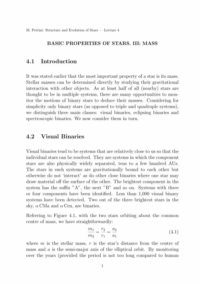
Referring to Figure 4.1, with the two stars orbiting about the commoncentre of mass, we have straightforwardly:

m1

m2=r2

r1=a2

a1(4.1)

where m is the stellar mass, r is the star’s distance from the centre ofmass and a is the semi-major axis of the elliptical orbit. By monitoringover the years (provided the period is not too long compared to human

1

m2r1

2a1

m1

Centre of Mass

r2

2a2

Figure 4.1: Schematic of a binary star system viewed face-on. In this example, m1 = 2m2.

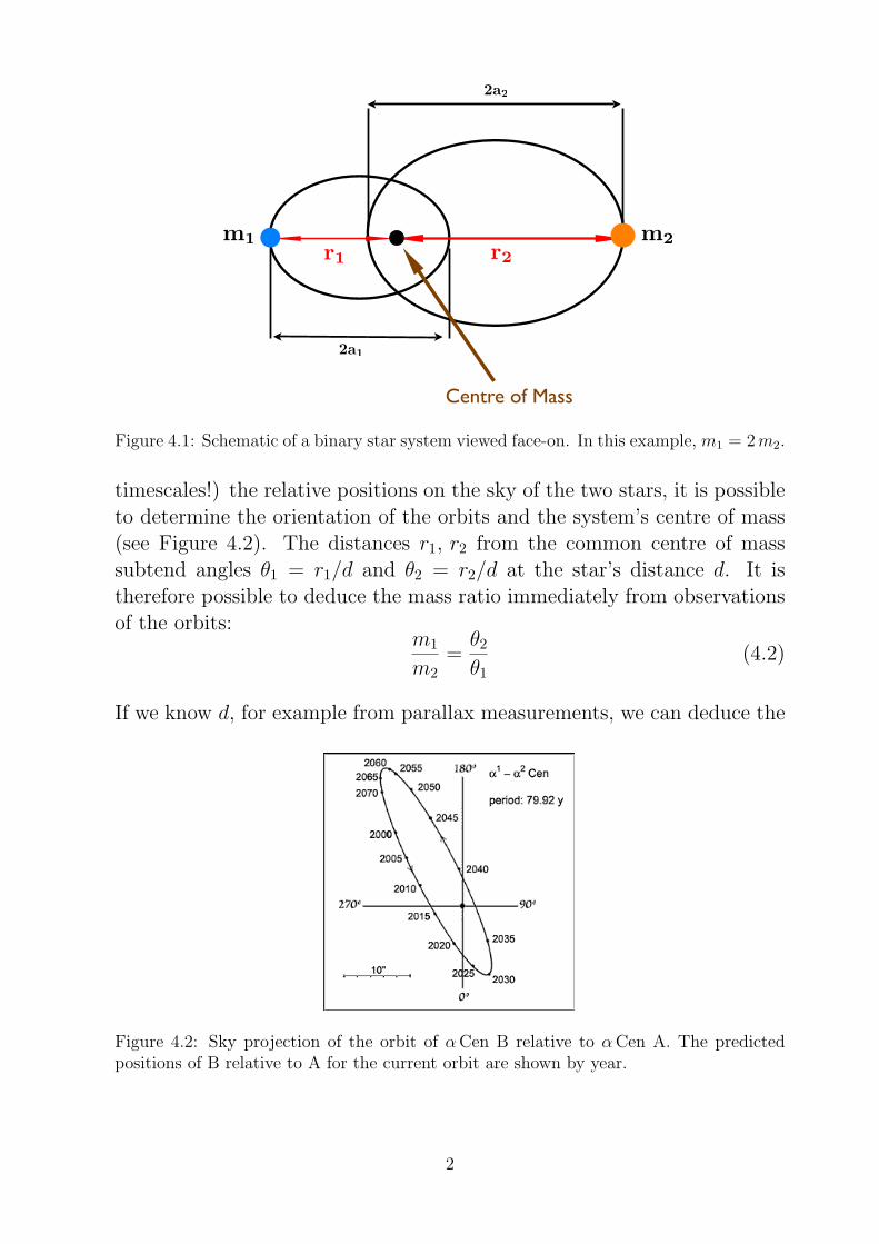
timescales!) the relative positions on the sky of the two stars, it is possibleto determine the orientation of the orbits and the system’s centre of mass(see Figure 4.2). The distances r1, r2 from the common centre of masssubtend angles θ1 = r1/d and θ2 = r2/d at the star’s distance d. It istherefore possible to deduce the mass ratio immediately from observationsof the orbits:

m1

m2=θ2

θ1(4.2)

If we know d, for example from parallax measurements, we can deduce the

Figure 4.2: Sky projection of the orbit of αCen B relative to αCen A. The predictedpositions of B relative to A for the current orbit are shown by year.

2

individual masses using Kepler’s third law:

P 2 =4π2

G (m1 +m2)a3 (4.3)

where P is the period (the same for both orbits) and a = a1 + a2 is thesemimajor axis of the orbit of the reduced mass µ,

µ =m1 ·m2

m1 +m2.

Recall that, in general, a two-body problem may be treated as an equivalentone-body problem with the reduced mass µ moving about a fixed massM = m1 +m2 at a distance r = |r2 − r1|.

In order to deduce m1 and m2 from observations of θ1, θ2 and P it isnecessary to correct for: (i) the parallax of the whole system, (ii) theproper motion of the centre of mass, and (iii) the inclination of the planeof the orbit relative to the plane of the sky. (i) is easy: just observe abinary system for more than one year cycle. (ii) is also relatively simple,since the centre of mass must move at constant velocity. (iii) is trickier.

Figure 4.3: The projection of an elliptical orbit inclined by the angle i to the plane of thesky is also an elliptical orbit. However, the real foci of the ellipse do not project to thefoci of the observed ellipese. (Reproduced from Carroll & Ostlie’s Modern Astrophysics).

3

Consider the special case where the orbital plane is inclined at angle i tothe plane of the sky (that is, it is inclined by an angle 90◦ − i to the lineof sight) and the two planes intersect along a line parallel to the minoraxis of the stellar orbit, forming a line of nodes, as in Figure 4.3. Whatwe observe in this case are angles θ′1 = θ1 cos i and θ′2 = θ2 cos i. Theunknown inclination doesn’t affect the estimate of the mass ratio, sincethe cos i factors cancel out in eq. 4.2. However, they can make a significantdifference in the estimate of a in eq. 4.3, which now becomes (solving forthe sum of the masses):

m1 +m2 =4π2

G

(θd)3

P 2 =4π2

G

(d

cos i

)3 θ′3

P 2 (4.4)

where θ is in radians and θ′ = θ′1 + θ′2.

Thus, in order to evaluate the sum of the masses properly, we need to knowthe angle of inclination i. This can be deduced by careful observation ofthe centre of mass which, as shown in Figure 4.3, will not coincide with thethe focus of the projected ellipse. The geometry of the true ellipse may bedetermined by comparing the observed stellar positions with mathematicalprojections of various ellipses onto the plane of the sky. The real situationis of course more complicated because in general the orbital plane may beinclined about both the minor and major axes.

In cases where the distance to a visual binary is not known, it may still bepossible to deduce a1 and a2 and solve for m1 and m2 using radial velocitymeasurements, which give the projections of the velocity vectors along theline of sight.

Several hundred visual pairs are known, but in most cases it has not yetbeen determined whether they are bound binary systems or chance super-positions. Many visual binaries have long orbital periods of several cen-turies or millennia and therefore have orbits which are uncertain or poorlyknown. For this reason, they only sample rather sparsely the HR diagram,with a strong bias towards the more common (and therefore more likelyto occur in the solar vicinity) low mass stars. Fortunately, other types ofbinary stars help us expand the range of reliable stellar mass determina-tions.

4

4.3 Spectroscopic Binaries

When two stars in a binary system are too far away to be resolved evenwith the largest telescopes on Earth, the binarity of the system can still beinferred from consideration of the spectrum, which will be the superposi-tion of two set of spectral features (which may be different if the stars are ofdifferent spectral types). In double-lined spectroscopic binaries, the absorp-tion lines in the composite spectrum will be seen to move in wavelength, aseach star moves in its orbit towards us and away from us (see Figure 4.4).The maximum blueshift and redshift we measure within an orbit are lowerlimits to the true velocities because of the unknown inclination i of theorbital plane to the line of sight: v1rmax = v1 sin i and v2rmax = v2 sin i.

Many spectroscopic binaries have nearly circular orbits because the timescalesof tidal interactions which tend to circularise the orbits are short comparedto the stellar lifetimes. When the eccentricities are small (ε � 1), the or-bital speed is essentially constant: v = 2πa/P and where P is the periodand the semi-major axis a is now the radius. Substituting into eq. 4.1, we

Figure 4.4: Schematic diagram of a double-lined spectroscopic binary, showing the orbitsand the resultant composite spectrum produced at different orbital phases. Note that thecentre of mass of the system has a radial velocity vr ' +15 km s−1 .

5

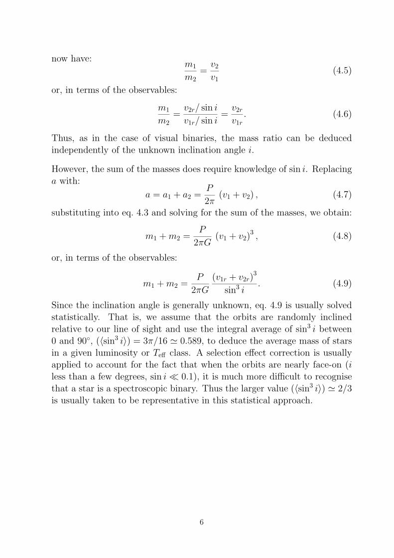
now have:m1

m2=v2

v1(4.5)

or, in terms of the observables:

m1

m2=v2r/ sin i

v1r/ sin i=v2r

v1r. (4.6)

Thus, as in the case of visual binaries, the mass ratio can be deducedindependently of the unknown inclination angle i.

However, the sum of the masses does require knowledge of sin i. Replacinga with:

a = a1 + a2 =P

2π(v1 + v2) , (4.7)

substituting into eq. 4.3 and solving for the sum of the masses, we obtain:

m1 +m2 =P

2πG(v1 + v2)

3 , (4.8)

or, in terms of the observables:

m1 +m2 =P

2πG

(v1r + v2r)3

sin3 i. (4.9)

Since the inclination angle is generally unknown, eq. 4.9 is usually solvedstatistically. That is, we assume that the orbits are randomly inclinedrelative to our line of sight and use the integral average of sin3 i between0 and 90◦, (〈sin3 i〉) = 3π/16 ' 0.589, to deduce the average mass of starsin a given luminosity or Teff class. A selection effect correction is usuallyapplied to account for the fact that when the orbits are nearly face-on (iless than a few degrees, sin i� 0.1), it is much more difficult to recognisethat a star is a spectroscopic binary. Thus the larger value (〈sin3 i〉) ' 2/3is usually taken to be representative in this statistical approach.

6

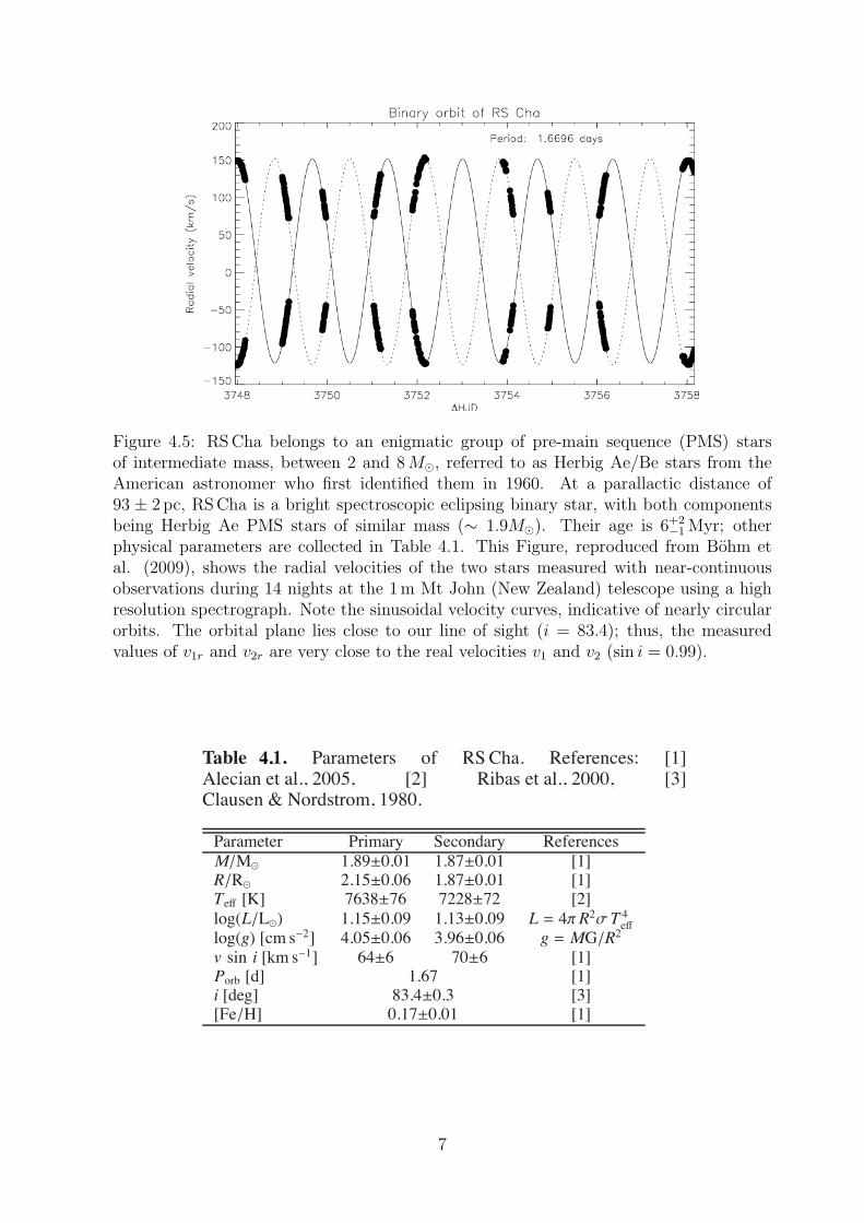
Figure 4.5: RS Cha belongs to an enigmatic group of pre-main sequence (PMS) starsof intermediate mass, between 2 and 8M�, referred to as Herbig Ae/Be stars from theAmerican astronomer who first identified them in 1960. At a parallactic distance of93 ± 2 pc, RS Cha is a bright spectroscopic eclipsing binary star, with both componentsbeing Herbig Ae PMS stars of similar mass (∼ 1.9M�). Their age is 6+2

−1 Myr; otherphysical parameters are collected in Table 4.1. This Figure, reproduced from Bohm etal. (2009), shows the radial velocities of the two stars measured with near-continuousobservations during 14 nights at the 1 m Mt John (New Zealand) telescope using a highresolution spectrograph. Note the sinusoidal velocity curves, indicative of nearly circularorbits. The orbital plane lies close to our line of sight (i = 83.4); thus, the measuredvalues of v1r and v2r are very close to the real velocities v1 and v2 (sin i = 0.99).

2 T. Bohm et al.: Discovery of non-radial pulsations in the spectroscopic binary Herbig Ae star RS Cha

tive phenomena. Even if the presence of complex fields can notbe ruled out it is of major importance to investigate other pos-sible external or internal origins of this tremendous amount ofdissipated energy, as witnessed by chromospheres and coronae,but also variable spectral lines, winds and bipolar jets.

The only way of studying in detail the internal stellarstructure is the analysis and the modelling of stellar pulsa-tions, if observed. As an example, PMS stars gain their en-ergy from gravitational contraction and therefore di!er signi-cantly from post-main-sequence stars having already processednuclear material - stellar pulsations are sensitive to these dif-ferences of internal stellar structure (see e.g. Suran et al., 2001).As of today, the internal stellar structure of PMS stars is notyet well constrained. Since few years the existence of pul-sating intermediate mass PMS stars is known (Breger, 1972;Kurtz & Marang, 1995; Donati et al., 1997). This observationalresult motivatedMarconi & Palla (Marconi & Palla, 1998) to in-vestigate the pulsation characteristics of HR5999 theoretically,which enabled them to predict the existence of a pre-main-sequence instability strip, which is being crossed by most ofthe intermediate mass PMS objects for a significant fraction oftheir evolution to the main sequence. This strip covers approxi-mately the same area in the HR diagram as the ! Scuti variables.Zwintz (Zwintz, 2008) compared, based on photometry, the ob-servational instability regions for pulsating pre-main sequenceand classical ! Scuti stars and concluded that the hot and coolboundaries of both HR diagram instability regions seem to co-incide. This preliminary result deserves further study by aim offull asteroseismological approach based on spectroscopy.

As of today, more than 30 intermediate-mass PMS starshave revealed to be pulsating at time-scales typical of ! Scutistars (see e.g. Kurtz & Marang, 1995; Kurtz & Catala, 2001;Donati et al., 1997; Bohm et al., 2004; Marconi et al., 2002;Ripepi & Marconi, 2003; Zwintz & Weiss, 2003; Catala, 2003and references therein).

RS Chamaeleontis is a bright spectroscopic eclipsing binarystar. Both components are Herbig Ae PMS stars of similar mass(close to 1.9 M!). Recently the age of RSCha has been de-termined to 6+2

"1Myr (Luhman & Steeghs, 2004), which verifies

it’s PMS nature. Andersen, 1975 already reported small ampli-tude radial velocity variations on top of the binary radial ve-locity curve for both components of RS Cha, suggesting thepossible presence of stellar pulsations. Photometric observationsby McInally & Austin, 1977 revealed short-term variations in atleast one of the two components, possibly linked to stellar pulsa-tions. Very recently, Alecian et al. (Alecian et al., 2005) reportedradial velocity variations in the residual velocity frame (cleanedfor orbital velocity) with amplitudes up to a few km s"1 and pe-riods of the order of 1h, indicative of ! Scuti type pulsations.

The aim of our study of the two components of RS Cha is toprovide a first set of asteroseismic constraints for forthcomingnon-radial pulsation models by determining unambiguously ahigher number of periodicities and identifying, in a second step,the corresponding pulsation modes with their respective degree" and azimuthal number m.

To achieve this goal, we decided to perform high resolutionspectroscopic observations on a large time basis and with opti-mized time coverage.

Section 2 reviews previous related work, Sect. 3 describesthe observations and data reduction, Sect. 4 summarizes resultsof the orbit determination, Sect. 5 reveals the detection of non-radial pulsations in both components of RS Cha, Sect. 6 and 7present frequency analysis and moment identification in the pri-

Table 1. Parameters of RSCha. References: [1]Alecian et al., 2005, [2] Ribas et al., 2000, [3]Clausen & Nordstrom, 1980.

Parameter Primary Secondary References

M/M! 1.89±0.01 1.87±0.01 [1]R/R! 2.15±0.06 1.87±0.01 [1]Te! [K] 7638±76 7228±72 [2]

log(L/L!) 1.15±0.09 1.13±0.09 L = 4#R2$T 4e!

log(g) [cm s"2] 4.05±0.06 3.96±0.06 g = MG/R2

v sin i [km s"1] 64±6 70±6 [1]Porb [d] 1.67 [1]i [deg] 83.4±0.3 [3][Fe/H] 0.17±0.01 [1]

Table 2. Log of the observations at Mt John Observatory,NZ, in Jan 2006. (1) and (2) Julian date (mean observation)(2,450,000+); (3) Number of high resolution RS Cha spectra;(4) typical range of S/N (pixel"1) at 550 nm (centre of V band)

Date JDfirst JDlast Nspec S/NRange(1) (2) (3) (4) (5)

Jan 09 3745.0101 1 120Jan 10 3745.9544 3745.9733 2 80-100Jan 12 3747.9537 3748.1779 28 70-90Jan 13 3749.0013 3749.1930 23 100-120Jan 14 3749.8911 3749.9911 12 70-90Jan 15 3750.8921 3751.1919 31 150Jan 16 3751.8958 3752.1970 29 90-120Jan 19 3754.9015 3755.2006 33 100-130Jan 20 3755.9245 3756.1993 25 90-120Jan 21 3756.9068 3757.0386 14 60-150Jan 22 3757.9004 3758.1621 32 120-170

mary and secondary component, respectively. A discussion isproposed and a conclusion is drawn in Section 8.

2. Previous related work

The pre-main sequence spectroscopic eclipsing binary RSCha has been studied extensively throughout the last years.Thanks to its eclipsing nature and the known inclination an-gle the system has fully been calibrated (Alecian et al., 2005,Alecian et al., 2007a, Alecian et al., 2007b). Table 1 summa-rizes the main results.

3. Observations

The analysis presented in this paper is based on a 14 nightsobserving run in January 2006 at the 1m Mt John telescopeequipped with the Hercules echelle spectrograph. We obtainedquasi-continuous single-site observations of the target star dur-ing these 2 weeks and obtained a total of 255 individual stel-lar echelle spectra, each spectrum having an individual exposuretime of 10min. The star was observed in high resolution spec-troscopy at R # 45000 and covering the wavelength area from457 to 704 nm, spread over 44 orders. The detector was a 1kx1kSite CCD. The highest S/N (pixel"1) values we obtained reached210 on Jan 16th, corresponding to almost 300 per resolved ele-ment (2 pixels); typical values of S/N (pixel"1) ranged around80-150 in this run. Table 2 summarizes the log of the observa-tions.

The general observing strategy was to obtain as many 10minute observations of the target star during the night as pos-

4.

7

Of much interest in astronomy are single-lined spectroscopic binaries. Theseare cases where only the spectrum of one of the pair is observed, but theperiodic variations in its radial velocity indicate the presence of an un-seen companion. This could be the case if: (a) the second star is verymuch fainter than the first—Sirius A and B are a good example; (b) thecompanion is a dark object, such as a neutron star or a black hole—suchsystems provide some of the most compelling evidence for the existence ofstellar-mass black holes; and (c) if the secondary is a planet. In this case,the radial velocity amplitudes are only m s−1, rather than km s−1.

In single-lined binaries, where we cannot measure v2r, we can substitutethe relation v2r = v1rm1/m2 (eq. 4.6) into eq. 4.9 to obtain:

m1 +m2 =P

2πG

v31r

sin3 i

(1 +

m1

m2

)3(4.10)

which can be rearranged in a form which groups together all the observableson the right-hand side of the equation:

m32

(m1 +m2)2 sin3 i =P

2πGv3

1r. (4.11)

The left-hand side of this equation is known as the mass function. Evenif m1 is not known, the mass function can still provide interesting lowerlimits to the mass of the unseen companion, since m1 > 0 and sin i ≤ 1,and therefore:

P

2πGv3

1r < m2 (4.12)

If the condition m2 � m1 is satisfied, which is the case of the secondarycomponent of the binary system is a planet, then m1 + m2 ≈ m1. Substi-tuting into 4.11, we now have:

m32 sin3 i ≈ P

2πGv3

1rm21 (4.13)

While there is still an inclination uncertainty for any particular system,statistical results can be obtained for large sample of stars with measuredoscillations attributable to planet-mass companions.

8

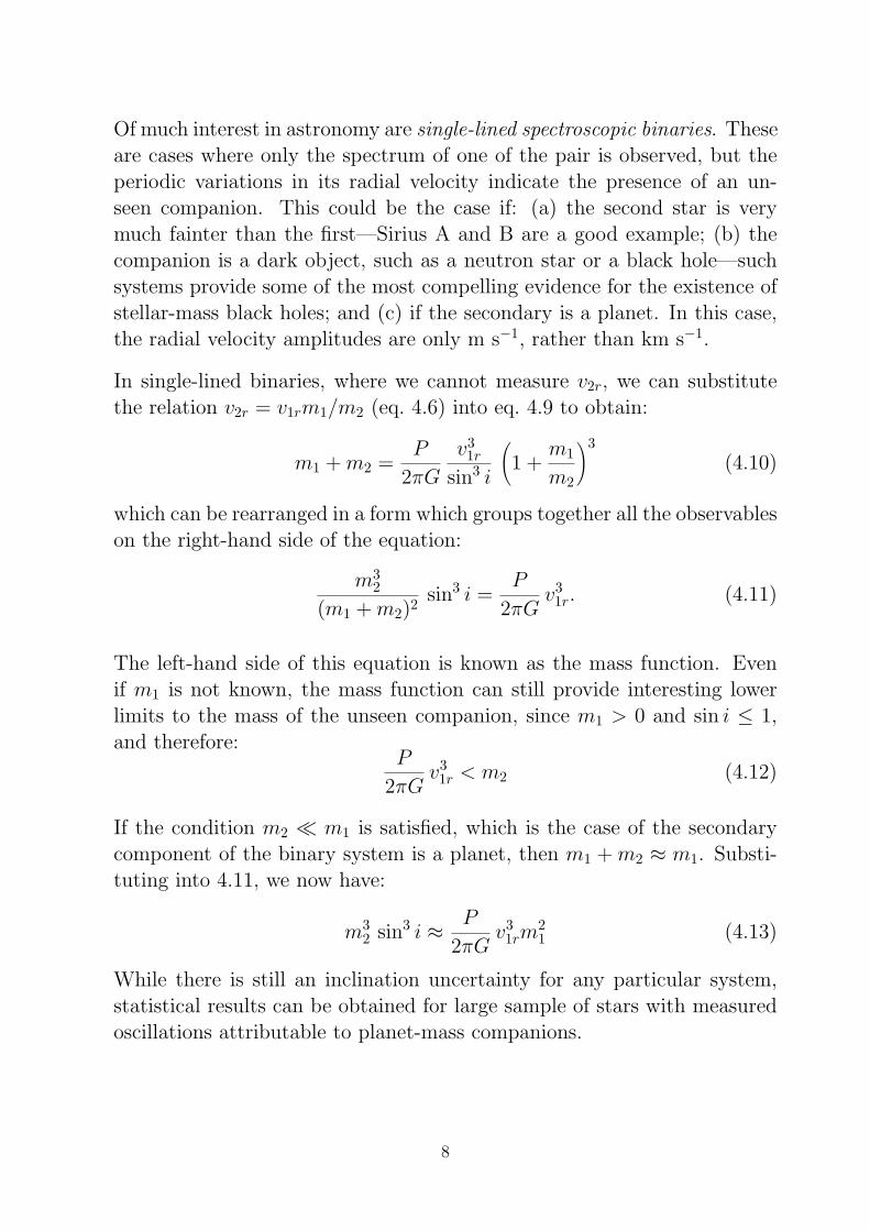
4.4 Eclipsing Binaries

The ambiguities associated with the unknown orientation can be removedin cases where we see occultations of one of the stars by the other. Providedthat the separation between the two stars is much greater than the sumof their radii (a condition which is not satisfied in contact binaries), thenit must be the case that the inclination of the orbital plane to the sky isclose to 90◦ (see Figure 4.6). Note also that for i > 75◦, sin i > 0.9, so thatthe error in the masses deduced with the assumption that i = 90◦ is lessthan 10%.

Comparing the light curves for the cases of complete (Figure 4.6) andpartial (Figure 4.7) eclipse, it can be appreciated that it is possible torecognise the cases where i < 90◦.

When the eclipse is total, we can deduce the radii of both stars fromaccurate timing of the phases of the eclipse. With the assumption thatthe smaller star is moving perpendicularly to our line of sight during theduration of the eclipse, its radius can be straightforwardly derived from

rs =v

2(tb − ta) (4.14)

where ta and tb are the times of first contact and minimum light respectively(see Figure 4.6) and v = vs + vl is the relative velocity of the two stars.

Figure 4.6: Schematic diagram of an eclipsing binary. The smaller star is assumed to behotter than the larger one. (Reproduced from Carroll & Ostlie’s Modern Astrophysics).

9

Figure 4.7: Schematic diagram of a partial eclipsing binary. The smaller star is assumed tobe hotter than the larger one. (Reproduced from Carroll & Ostlie’s Modern Astrophysics).

Similarly:

rl =v

2(tc − ta) = rs +

v

2(tc − tb) (4.15)

The light curve of eclipsing binaries gives information not only on the radiiof the two stars but also on the ratio of their effective temperatures. Thisfollows directly from eq. 2.13, L = 4πR2σT 4; as when an area πR2 iseclipsed from the system, the drop in flux will be different depending onwhether the hotter star of the two is in front or behind the cooler one (seeFigure 4.6). Assuming for simplicity a uniform flux across the stellar disk,we have:

F0 = A(πR2

lF′l + πR2

sF′s

)(4.16)

where F ′ is the radiative surface flux, F0 is the measured flux when there isno eclipse, and A is a proportionality constant to account for the fact thatwe register only a fraction of the flux emitted (due to distance, interveningabsorption and limited efficiency of the instrumentation). The deeper, orprimary, minimum in the light curve occurs when the hotter star is eclipsedby the cooler one. In the example shown in Figure 4.6, this is the smallerstar. Then, during the primary minimum we have:

F1 = AπR2lF′l , (4.17)

while during the secondary minimum:

F2 = A(πR2

l − πR2s

)F ′l + AπR2

sF′s . (4.18)

10

1983Obs...103...29S

L

L!!

!M

M!

"4L

L!!

!M

M!

"2.3

R C Smith 1983

Figure 4.8: The empirical stellar mass-luminosity relation constructed from observationsof different types of binary stars (from Smith 1983).

To circumvent uncertainties in the constant A, we concern ourselves withthe ratio of the two fluxes:

F0 − F1

F0 − F2=F ′sF ′l

=

(Ts

Tl

)4

(4.19)

What eq. 4.19 tells us is that the ratio of the measured fluxes during theprimary and secondary eclipses gives a direct measure of the ratio of theeffective temperatures of the two stars in the eclipsing binary system.

4.5 The Stellar Mass-Luminosity Relation

When we bring together the best determinations of stellar masses fromdifferent types of binary stars, we find a well defined mass-luminosity re-lation for hydrogen burning dwarfs. Figure 4.8 shows the empirical mass-luminosity relation constructed from data available in the late 1970s-early1980s. Thirty years later, the number of stars with direct measurements ofmass and radius has increased considerably, thanks in part to the adventof long-baseline optical interferometry which can resolve the stellar disks.Figure 4.9, reproduced from the review by Torres et al. 2010 (A&ARv,

11

L !M3.5

Figure 4.9: The empirical stellar mass-luminosity relation from observations of 190 starsin 95 detached binary systems, all with masses and radii known with an accuracy of 3%or better (data from Torres et al. 2010).

18, 67), is a compilation of measurements for 95 detached binary systemscontaining 190 stars satisfying the criterion that the mass and radius ofboth stars be known with an accuracy of 3% or better.

Any theory of stellar structure must be able to reproduce such a relation inorder to be deemed valid; we shall return to this point in Lecture 10. Herewe limit ourselves to some preliminary considerations. First of all, such aclear-cut M − L relation provides a natural explanation for the existenceof a prominent main sequence in the HR diagram. After forming withina collapsing interstellar cloud, stars begin their hydrogen-burning lives onthe main sequence, at a location on the MV –(B − V ) plane determined bytheir mass. Stars do not evolve along the main sequence, they evolve offthe main sequence.

A rough approximation to the slope of the mass-luminosiy relation overthe full range of stellar masses is L ∝M∼3.5. If stars shine through nuclearfusion, we can write:

dM

dt= k L

where L is the luminosity and k is a constant of proportionality. Integrat-ing, we have:

t ∝ M

L∝ M

M 3.5 ∝M−2.5 .

12

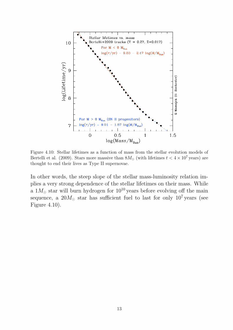
Figure 4.10: Stellar lifetimes as a function of mass from the stellar evolution models ofBertelli et al. (2009). Stars more massive than 8M� (with lifetimes t < 4× 107 years) arethought to end their lives as Type II supernovae.

In other words, the steep slope of the stellar mass-luminosity relation im-plies a very strong dependence of the stellar lifetimes on their mass. Whilea 1M� star will burn hydrogen for 1010 years before evolving off the mainsequence, a 20M� star has sufficient fuel to last for only 107 years (seeFigure 4.10).

13