Embed Size (px)
Citation preview

This page intentionally left blank
Dynamics of Particles and Rigid Bodies: A Systematic Approach
Dynamics of Particles and Rigid Bodies: A Systematic Approach is intended for under-graduate courses in dynamics. This work is a unique blend of conceptual, theoretical,and practical aspects of dynamics generally not found in dynamics books at the un-dergraduate level. In particular, in this book the concepts are developed in a highlyrigorous manner and are applied to examples using a step-by-step approach that iscompletely consistent with the theory. In addition, for clarity, the notation used to de-velop the theory is identical to that used to solve example problems. The result of thisapproach is that a student is able to see clearly the connection between the theory andthe application of theory to example problems. While the material is not new, instruc-tors and their students will appreciate the highly pedagogical approach that aids inthe mastery and retention of concepts. The approach used in this book teaches a stu-dent to develop a systematic approach to problem solving. The work is supported bya great range of examples and reinforced by numerous problems for student solution.An instructor’s solutions manual is available.
Anil V. Rao earned his B.S. in mechanical engineering and A.B. in mathematics fromCornell University, his M.S.E. in aerospace engineering from the University of Michi-gan, and his M.A. and Ph.D. in mechanical and aerospace engineering from PrincetonUniversity. After earning his Ph.D., Dr. Rao joined the Flight Mechanics Department atThe Aerospace Corporation in Los Angeles, where he was involved in mission supportfor U.S. Air Force launch vehicle programs and trajectory optimization software devel-opment. Subsequently, Dr. Rao joined The Charles Stark Draper Laboratory, Inc., inCambridge, Massachusetts. Since joining Draper, Dr. Rao has been involved in numer-ous projects related to trajectory optimization, guidance, and navigation of aerospacevehicles. Concurrently, for the past several years Dr. Rao has been an Adjunct Pro-fessor of Aerospace and Mechanical Engineering at Boston University where he hastaught the core undergraduate engineering dynamics course. Since joining BU, Dr. Raohas been voted AIAA/ASME Faculty Member of the Year Award by the Aerospace andMechanical Engineering Department and has been voted Boston University College ofEngineering Professor of the Year for outstanding teaching.

DYNAMICSOF PARTICLES AND RIGID BODIES
A SYSTEMATIC APPROACH
ANIL V. RAO
Boston University
CAMBRIDGE UNIVERSITY PRESS
Cambridge, New York, Melbourne, Madrid, Cape Town, Singapore, São Paulo
Cambridge University PressThe Edinburgh Building, Cambridge CB2 8RU, UK
First published in print format
ISBN-13 978-0-521-85811-3
ISBN-13 978-0-511-34840-2
© Anil Vithala Rao 2006
Image on cover: courtesy NASA/JPL-Caltech. Fig. 1–4 Used by permission of DiracDeltaConsultants, UK. Fig. 3–3 adapted from Figure 4.6 on page 49 of O. O’Reilly, Engineering Dynamics: A Primer, 2001 by permission of Oliver O’Reilly and Springer-Verlag, Heidelberg, Germany. Drawing of bulldozer appearing in Fig. P5-3 used by permission of the artist, Richard Neuman (URL: http://www.richard-neuman-artist.com).Questions 3.9, 5.1, 5.7, 5.11, and 5.15 and Examples 5–10, 5–8, and 5–17 adapted fromGreenwood, D. T., Principles of Dynamics,2nd Edition, 1987, by permission of Donald T. Greenwood and Pearson Education, Inc., Upper Saddle River, NJ (Pearson EducationReference Number: 103682). The illustrations in this manuscript were created using CorelDRAW Version 12. CorelDRAW is a registered trademark of Corel Corporation, 1600 Carling Avenue, Ottawa, Ontario K1Z 8R7, Canada. This manuscript was typeset
using the MikTeX version of LATEX2 using the Lucida Bright Math, Lucida New Math,and Lucida Bright Math Expert fonts manufactured by Y & Y, Inc., 106 Indian Hill, Carlisle, MA, 01741, USA.
1906
Information on this title: www.cambridge.org/9780521858113
This publication is in copyright. Subject to statutory exception and to the provision of relevant collective licensing agreements, no reproduction of any part may take place without the written permission of Cambridge University Press.
ISBN-10 0-511-34840-1
ISBN-10 0-521-85811-9
Cambridge University Press has no responsibility for the persistence or accuracy of urls for external or third-party internet websites referred to in this publication, and does not guarantee that any content on such websites is, or will remain, accurate or appropriate.
Published in the United States of America by Cambridge University Press, New York
www.cambridge.org
hardback
eBook (EBL)
eBook (EBL)
hardback
Vakratunda Mahaakaaya Soorya Koti SamaprabhaNirvighnam Kuru Mein Deva Sarva Kaaryashu Sarvadaa
I dedicate this book with love to Anita and Vikramand to my parents, Saroj and Rajeswara

Contents
Preface ix
Acknowledgments xiii
Nomenclature xv
1 Introductory Concepts 11.1 Scalars . . . . . . . . . . . . . . . . . . . . . . . . . . . . . . . . . . . . . . . . . . 21.2 Vectors . . . . . . . . . . . . . . . . . . . . . . . . . . . . . . . . . . . . . . . . . . 31.3 Tensors . . . . . . . . . . . . . . . . . . . . . . . . . . . . . . . . . . . . . . . . . 101.4 Matrices . . . . . . . . . . . . . . . . . . . . . . . . . . . . . . . . . . . . . . . . . 141.5 Ordinary Differential Equations . . . . . . . . . . . . . . . . . . . . . . . . . . . 25
2 Kinematics 272.1 Reference Frames . . . . . . . . . . . . . . . . . . . . . . . . . . . . . . . . . . . 282.2 Coordinate Systems . . . . . . . . . . . . . . . . . . . . . . . . . . . . . . . . . . 302.3 Rate of Change of Scalar and Vector Functions . . . . . . . . . . . . . . . . . 322.4 Position, Velocity, and Acceleration . . . . . . . . . . . . . . . . . . . . . . . . 352.5 Degrees of Freedom of a Particle . . . . . . . . . . . . . . . . . . . . . . . . . . 372.6 Relative Position, Velocity, and Acceleration . . . . . . . . . . . . . . . . . . . 392.7 Rectilinear Motion . . . . . . . . . . . . . . . . . . . . . . . . . . . . . . . . . . . 392.8 Using Noninertial Reference Frames to Describe Motion . . . . . . . . . . . 422.9 Rate of Change of a Vector in a Rotating Reference Frame . . . . . . . . . . 422.10 Kinematics in a Rotating Reference Frame . . . . . . . . . . . . . . . . . . . . 502.11 Common Coordinate Systems . . . . . . . . . . . . . . . . . . . . . . . . . . . . 512.12 Kinematics in a Rotating and Translating Reference Frame . . . . . . . . . 852.13 Practical Approach to Computing Velocity and Acceleration . . . . . . . . . 882.14 Kinematics of a Particle in Continuous Contact with a Surface . . . . . . . 992.15 Kinematics of Rigid Bodies . . . . . . . . . . . . . . . . . . . . . . . . . . . . . 104Summary of Chapter 2 . . . . . . . . . . . . . . . . . . . . . . . . . . . . . . . . . . . 126Problems for Chapter 2 . . . . . . . . . . . . . . . . . . . . . . . . . . . . . . . . . . . 130
3 Kinetics of Particles 1453.1 Forces Commonly Used in Dynamics . . . . . . . . . . . . . . . . . . . . . . . 1463.2 Inertial Reference Frames . . . . . . . . . . . . . . . . . . . . . . . . . . . . . . 1563.3 Newton’s Laws for a Particle . . . . . . . . . . . . . . . . . . . . . . . . . . . . . 1573.4 Comments on Newton’s Laws . . . . . . . . . . . . . . . . . . . . . . . . . . . . 1573.5 Examples of Application of Newton’s Laws in Particle Dynamics . . . . . . 158

viii Contents
3.6 Linear Momentum and Linear Impulse for a Particle . . . . . . . . . . . . . . 1763.7 Moment of a Force and Moment Transport Theorem for a Particle . . . . . 1783.8 Angular Momentum and Angular Impulse for a Particle . . . . . . . . . . . 1793.9 Instantaneous Linear and Angular Impulse . . . . . . . . . . . . . . . . . . . 1873.10 Power, Work, and Energy for a Particle . . . . . . . . . . . . . . . . . . . . . . 188Summary of Chapter 3 . . . . . . . . . . . . . . . . . . . . . . . . . . . . . . . . . . . 218Problems for Chapter 3 . . . . . . . . . . . . . . . . . . . . . . . . . . . . . . . . . . . 222
4 Kinetics of a System of Particles 2374.1 Center of Mass and Linear Momentum of a System of Particles . . . . . . . 2384.2 Angular Momentum of a System of Particles . . . . . . . . . . . . . . . . . . 2404.3 Newton’s 2nd Law for a System of Particles . . . . . . . . . . . . . . . . . . . 2424.4 Moment of a System of Forces Acting on a System of Particles . . . . . . . 2484.5 Rate of Change of Angular Momentum for a System of Particles . . . . . . 2494.6 Impulse and Momentum for a System of Particles . . . . . . . . . . . . . . . 2664.7 Work and Energy for a System of Particles . . . . . . . . . . . . . . . . . . . . 2804.8 Collision of Particles . . . . . . . . . . . . . . . . . . . . . . . . . . . . . . . . . 289Summary of Chapter 4 . . . . . . . . . . . . . . . . . . . . . . . . . . . . . . . . . . . 305Problems for Chapter 4 . . . . . . . . . . . . . . . . . . . . . . . . . . . . . . . . . . . 310
5 Kinetics of Rigid Bodies 3215.1 Center of Mass and Linear Momentum of a Rigid Body . . . . . . . . . . . . 3225.2 Angular Momentum of a Rigid Body . . . . . . . . . . . . . . . . . . . . . . . . 3235.3 Moment of Inertia Tensor of a Rigid Body . . . . . . . . . . . . . . . . . . . . 3255.4 Principal-Axis Coordinate Systems . . . . . . . . . . . . . . . . . . . . . . . . . 3345.5 Actions on a Rigid Body . . . . . . . . . . . . . . . . . . . . . . . . . . . . . . . 3495.6 Moment Transport Theorem for a Rigid Body . . . . . . . . . . . . . . . . . . 3535.7 Euler’s Laws for a Rigid Body . . . . . . . . . . . . . . . . . . . . . . . . . . . . 3555.8 Systems of Rigid Bodies . . . . . . . . . . . . . . . . . . . . . . . . . . . . . . . 3915.9 Rotational Dynamics of a Rigid Body Using Moment of Inertia . . . . . . . . 4105.10 Work and Energy for a Rigid Body . . . . . . . . . . . . . . . . . . . . . . . . . 4195.11 Impulse and Momentum for a Rigid Body . . . . . . . . . . . . . . . . . . . . 4415.12 Collision of Rigid Bodies . . . . . . . . . . . . . . . . . . . . . . . . . . . . . . . 450Summary of Chapter 5 . . . . . . . . . . . . . . . . . . . . . . . . . . . . . . . . . . . 467Problems for Chapter 5 . . . . . . . . . . . . . . . . . . . . . . . . . . . . . . . . . . . 472
Appendices 486
A Principle-Axis Moments of Inertia of Homogeneous Bodies 487
B Identities, Derivatives, Integrals, and Gradient 493B.1 Identities . . . . . . . . . . . . . . . . . . . . . . . . . . . . . . . . . . . . . . . . . 493B.2 Derivatives and Integrals . . . . . . . . . . . . . . . . . . . . . . . . . . . . . . . 493B.3 Gradient of a Scalar Function . . . . . . . . . . . . . . . . . . . . . . . . . . . . 494
C Answers to Selected Problems 497
Bibliography 503
Index 505
Preface
The subject of dynamics has been taught in engineering curricula for decades, tradi-tionally as a second-semester course as part of a year-long sequence in engineeringmechanics. This approach to teaching dynamics has led to a wide array of currentlyavailable engineering mechanics books, including Beer and Johnston (1997), Bedfordand Fowler (2005), Hibbeler (2001), and Merriam and Kraige (1997). From my experi-ence, the reasons these books are adopted for undergraduate courses in engineeringmechanics are threefold. First, they include a wide variety of worked examples andhave more than 1000 problems for the students to solve at the end of each chapter.The variety of problems provides instructors with the flexibility to assign differentproblems every semester for several years. Second, these books are generic enoughthat they can be used to teach undergraduates in virtually any branch of engineering.Third, they cover both statics and dynamics, thereby making it is possible for a studentto purchase a single book for a year-long engineering mechanics course. Using theseempirical measures, it is hard to dispute that these books cover a tremendous amountof material and enable an instructor to tailor the material to the needs of a particularcourse. Given the vast array of undergraduate dynamics books already available, anobvious question that arises is, why write yet another book on the subject of under-graduate engineering dynamics? While it is clear that the availability of another bookon the subject would clearly add to the number of choices available to instructors, itmay be difficult at first glance to see how the addition of another book would add valueto the existing literature. However, after my experience over the past several years ofteaching dynamics, not only do I now believe that there is room for another book, butI feel strongly that the paradigm used to teach the subject of dynamics needs to becompletely overhauled.
Before I ever taught undergraduate dynamics, I, too, believed that the existing bookson engineering mechanics were more than adequate and that an additional book wouldadd little to no value to the existing literature. Consequently, without giving it muchthought, the first time I taught engineering dynamics (course EK302 at Boston Univer-sity) I randomly chose one of the standard undergraduate textbooks. Given my notionsat the time, it never occurred to me that the book I chose for my class would pose somany difficulties for my students. However, not more than a few weeks into my firstsemester of teaching, I was met by vehement complaints from my students regardingthe textbook. Given their frustration and my sincere desire to keep them motivated, Ibegan investigating more thoroughly why my students found the textbook so difficultto follow and what I could do to help them overcome their frustration.
My investigation began by carefully reading each of the aforementioned engineeringmechanics textbooks. My conclusion from reading these books was that the frustrationmy students were experiencing emanated from two sources. First, I found an enormous
x Preface
inconsistency between the presentation of the theory and the application of the theoryto examples. Second, I found the approach to problem solving was highly formulaicand did not place an emphasis on understanding. Essentially, I concluded that thesebooks lacked the pedagogy required for a student to master the key concepts and, in-stead, promoted an ad hoc approach to problem solving. More importantly, because ofthe inconsistency between the presentation and the application of the theory, I foundthat these books make it difficult for a student’s understanding of the material to growas the course progressed. Consequently, rather than solving problems systematicallyfrom first principles, my students were trying to solve homework problems either byemulating a problem solved in the book, by reverse engineering a solution using theanswers at the back of the book (by analogy to a boundary-value problem, I call thisapproach the “shooting” method for finding a solution to a problem), or by searchingfor formulas from which they could “plug in” the information that they are given. Theworst part was that, given a new problem (however similar it may appear to be to pre-vious problems), they were at a loss as to how to proceed because they had not trulyunderstood the key concepts.
My desire to write this book has grown out of my experience that undergraduateengineering dynamics needs to be taught in an extremely systematic and highly ex-plicit manner. My approach has been put to the test over the past several years whileteaching the core undergraduate engineering dynamics course at Boston University. Iconsider my approach to dynamics to be a significant departure from any of the ex-isting books on undergraduate engineering dynamics. First, different from the afore-mentioned books, I have developed a highly rigorous presentation of the concepts.Second, the level of rigor in solving problems is identical to that used in developingthe theory. Using my approach, it is possible for a student to see clearly the connec-tion between the theory and the application of the theory. To this end, I have adopteda more advanced (but what I believe is a significantly more descriptive) notation thanis commonly found in other undergraduate engineering dynamics books. Third, I havekept the material at the undergraduate level, i.e., the types of problems that are in-cluded share similarities with those found in many other engineering dynamics books.With regard to notation, with the exception of second-order tensors, the only mathe-matical prerequisite for this book is vector calculus (with regard to tensors, I believethat, given a few simple explanations and without losing a step, the basics of tensoralgebra can be handled by a fourth-semester undergraduate student in mechanical oraerospace engineering). Fourth, in absolutely every topic covered in this book, I usea step-by-step vector mechanics approach to solving problems. I have found throughexperience that the approach I have chosen works extremely well in practice. In partic-ular, I am able to see substantial growth in the thought process of my students fromthe first week of class to the final exam.
This book is intended for undergraduate students who want a systematic and rig-orous approach to the subject of particle and rigid body dynamics. Because of theintended audience, certain topics in this book have been intentionally omitted. In par-ticular, I do not cover the topics of systems where mass is gained or lost. Furthermore,I cover three-dimensional kinetics of rigid bodies in a relatively limited manner. In thecase of systems that gain or lose mass, to teach this topic correctly requires a basiccourse on fluid mechanics, which many students do not have upon entering an un-dergraduate engineering dynamics course. With regard to three-dimensional kineticsof a rigid body, it is simply not possible to cover this entire topic in a one-semesterundergraduate engineering dynamics course.
Preface xi
The material presented in this book is not new. However, I believe strongly that myapproach is highly pedagogical, truly aids in mastering the key concepts, and promotesretention of the material well beyond the duration of the course. As I have alreadysaid, my approach is a significant departure from approaches used in other books. Tomotivate my approach, I have attempted throughout the book to include a sufficientnumber of worked examples and have included a wide range of problems at the endof each chapter for a student to solve. Most of the problems are ones that I haveconstructed myself while others are based on problems from the beautifully writtenbook by Greenwood (1988). Finally, the notation I have adopted for kinematics is basedon the notation developed by Kane and Levinson (1985).
Finally, I would like to re-emphasize that this book has been written with the stu-dent in mind. To this end, everywhere possible I have attempted to provide explicitguidance so that the student is able to follow clearly both the theory and the examples.It is my sincere hope that students everywhere will benefit from this book.
Anil V. RaoBoston, Massachusetts

Acknowledgments
Writing a textbook is an arduous task and I have many people to acknowledge for theirinspiration and support. First, I am indebted to all of the teachers I have had in mylife, but particularly to my high school calculus teacher, Mr. David Bock, for giving methe inspiration to want to be a teacher, and to my Ph.D. thesis advisor, Dr. KennethD. Mease, for encouraging me to develop a rigorous approach to research and forteaching me by example the true value of expressing my thoughts in as clear a manneras possible.
With regard to the evolution of this book, I acknowledge my friend and colleague,Dr. Scott Ploen, for helping me greatly to improve both my perspective on the sub-ject of dynamics and to develop pedagogical approaches to motivate students to learnthe subject. I also acknowledge my former students, Theresia Becker and Kimber-ley Clarke, for taking enormous amounts of time and effort to carefully examine themanuscript for typographical errors and for providing helpful suggestions for improv-ing the discussions in the text. Next, I would like to thank my friend, Mr. DavidWoffinden, and my teaching assistants, Christophe Lecomte and Josh Burnett, for pro-viding me with valuable feedback about the content, style, and clarity of the manuscript.In addition, I would like to acknowledge Dr. John G. Papastivridis for his help in ob-taining an accurate historical reference to the parallel-axis theorem. Finally, I gratefullyacknowledge Dr. Donald T. Greenwood, Dr. Oliver M. O’Reilly, and Dr. David Geller fortaking the time to carefully read and provide constructive criticism of the manuscript.I particularly thank Dr. O’Reilly for helping me gain insight into the Euler basis and thedual Euler basis and for helping me arrive at an accurate description of a conservativetorque.
With regard to making this book a possibility, I owe a special acknowledgment toDr. John Baillieul for giving me the opportunity to teach at Boston University. WithoutDr. Baillieul’s help, I would never have been able to do something that has turned outto be so fulfilling and would never have had the opportunity, let alone the inspiration,to write this book.
I also thank my dear parents, Saroj and Rajeswara, whose lifelong efforts made itpossible for me to obtain a high quality education and have made a work such as thisa reality. Finally, I thank my beloved wife, Anita, for her encouragement and supportduring the time when I was working on this manuscript. I realize only now just howmuch time my writing this book took from other things in our lives, and I am gratefulfor her patience throughout this long endeavor.
Anil V. RaoBoston, Massachusetts

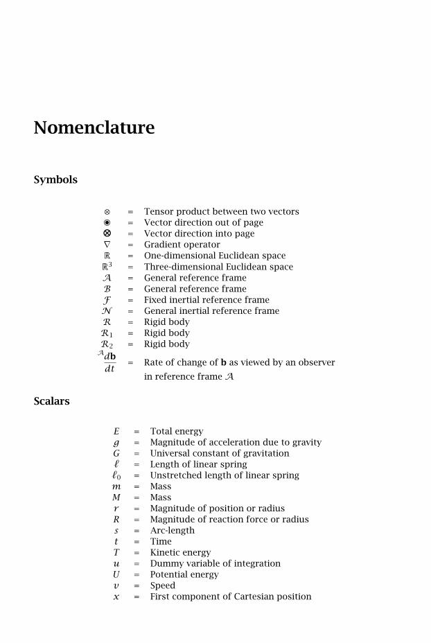
Nomenclature
Symbols
⊗ = Tensor product between two vectors• = Vector direction out of page⊗ = Vector direction into page∇ = Gradient operatorR = One-dimensional Euclidean spaceR3 = Three-dimensional Euclidean spaceA = General reference frameB = General reference frameF = Fixed inertial reference frameN = General inertial reference frameR = Rigid bodyR1 = Rigid bodyR2 = Rigid bodyAdbdt
= Rate of change of b as viewed by an observer
in reference frame A
Scalars
E = Total energyg = Magnitude of acceleration due to gravityG = Universal constant of gravitation = Length of linear spring0 = Unstretched length of linear springm = MassM = Massr = Magnitude of position or radiusR = Magnitude of reaction force or radiuss = Arc-lengtht = TimeT = Kinetic energyu = Dummy variable of integrationU = Potential energyv = Speedx = First component of Cartesian position
xvi Nomenclature
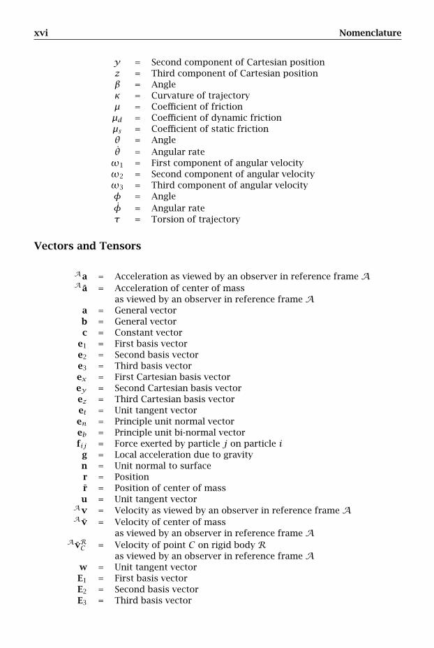
y = Second component of Cartesian positionz = Third component of Cartesian positionβ = Angleκ = Curvature of trajectoryµ = Coefficient of frictionµd = Coefficient of dynamic frictionµs = Coefficient of static frictionθ = Angleθ = Angular rateω1 = First component of angular velocityω2 = Second component of angular velocityω3 = Third component of angular velocityφ = Angleφ = Angular rateτ = Torsion of trajectory
Vectors and Tensors
Aa = Acceleration as viewed by an observer in reference frame AA a = Acceleration of center of mass
as viewed by an observer in reference frame Aa = General vectorb = General vectorc = Constant vector
e1 = First basis vectore2 = Second basis vectore3 = Third basis vectorex = First Cartesian basis vectorey = Second Cartesian basis vectorez = Third Cartesian basis vectoret = Unit tangent vectoren = Principle unit normal vectoreb = Principle unit bi-normal vectorfij = Force exerted by particle j on particle ig = Local acceleration due to gravityn = Unit normal to surfacer = Positionr = Position of center of massu = Unit tangent vector
Av = Velocity as viewed by an observer in reference frame AA v = Velocity of center of mass
as viewed by an observer in reference frame AAvRC = Velocity of point C on rigid body R
as viewed by an observer in reference frame Aw = Unit tangent vectorE1 = First basis vectorE2 = Second basis vectorE3 = Third basis vector
Nomenclature xvii
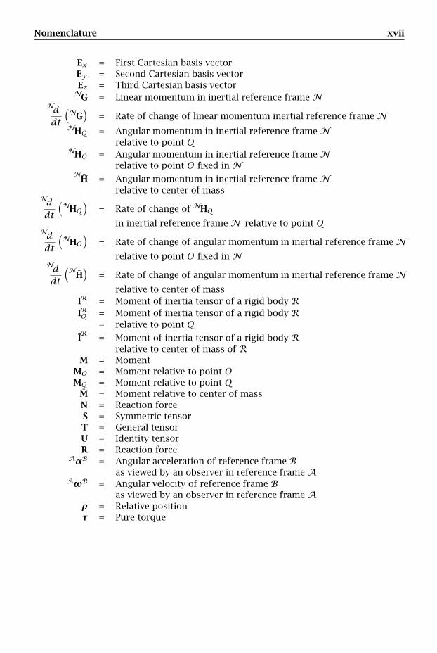
Ex = First Cartesian basis vectorEy = Second Cartesian basis vectorEz = Third Cartesian basis vectorNG = Linear momentum in inertial reference frame N
Nddt
(NG
)= Rate of change of linear momentum inertial reference frame N
NHQ = Angular momentum in inertial reference frame Nrelative to point Q
NHO = Angular momentum in inertial reference frame Nrelative to point O fixed in N
NH = Angular momentum in inertial reference frame N
relative to center of massNddt
(NHQ
)= Rate of change of NHQ
in inertial reference frame N relative to point QNddt
(NHO
)= Rate of change of angular momentum in inertial reference frame N
relative to point O fixed in NNddt
(NH)
= Rate of change of angular momentum in inertial reference frame Nrelative to center of mass
IR = Moment of inertia tensor of a rigid body RIRQ = Moment of inertia tensor of a rigid body R
= relative to point QIR
= Moment of inertia tensor of a rigid body Rrelative to center of mass of R
M = MomentMO = Moment relative to point OMQ = Moment relative to point Q
M = Moment relative to center of massN = Reaction forceS = Symmetric tensorT = General tensorU = Identity tensorR = Reaction force
AαB = Angular acceleration of reference frame Bas viewed by an observer in reference frame A
AωB = Angular velocity of reference frame Bas viewed by an observer in reference frame A
ρ = Relative positionτ = Pure torque

Chapter 1
Introductory Concepts
The scientist does not study nature because it is useful; he studies it becausehe delights in it, and he delights in it because it is beautiful. If nature werenot beautiful, it would not be worth knowing, and if nature were not worthknowing, life would not be worth living.
- Jules Henri Poincare (1854–1912)French Mathematician and Physicist
Mechanics is the study of the effect that physical forces have on objects. Dynamicsis the particular branch of mechanics that deals with the study of the effect that forceshave on the motion of objects. Dynamics is itself divided into two branches calledNewtonian dynamics and relativistic dynamics. Newtonian dynamics is the study ofthe motion of objects that travel with speeds significantly less than the speed of lightwhile relativistic dynamics is the study of the motion of objects that travel with speedsat or near the speed of light. This division in the subject of dynamics arises because thephysics associated with the motion of objects that travel with speeds much less thanthe speed of light can be modeled much more simply than the physics associated withthe motion of objects that travel with speeds at or near the speed of light. Moreover,nonrelativistic dynamics deals primarily with the motion of objects on a macroscopicscale while relativistic dynamics deals with the study of the motion of objects on amicroscopic or submicroscopic scale. The objective of this book is to present theunderlying concepts of Newtonian dynamics in a clear and concise manner and todevelop a systematic framework for solving problems in classical Newtonian dynamics.
As with any subject that is based on the laws of physics, Newtonian dynamics needsto be described using mathematics. More specifically, it must be possible to describethe physical laws in a way that is independent of the particular coordinate system inwhich one chooses to formulate a particular problem. The mathematical approach thatgives us the freedom to develop a coordinate-free approach to Newtonian mechanicsis that of vector and tensor algebra.
Once the physical laws have been described in a coordinate-free manner, the nextstep is to formulate the particular problem of interest. While the basic laws them-selves are coordinate-free, to solve a particular problem it is necessary to specify allrelevant quantities using a coordinate system of choice. While in principle it is possi-ble to use any coordinate system to describe the motion of a material body, choosing
2 Chapter 1. Introductory Concepts
a particular coordinate system could vastly simplify the particular problem under con-sideration. The remainder of this chapter is devoted to providing a review of the vectorand tensor algebra required to formulate and analyze problems in nonrelativistic me-chanics. While this chapter provides a mathematical overview, it is not intended as asubstitute for a book on engineering mathematics. For a more in-depth presentationof engineering mathematics, the reader is referred to a standard text in undergraduateengineering mathematics such as that found in Kreyszig (1988).
1.1 Scalars
A scalar is any quantity that is expressible as a real number. We denote a scalar by anon-boldface character and denote the set of real numbers by R, i.e., we say that the(non-boldface) quantity a is a scalar if
a ∈ R
Scalars satisfy the following properties with respect to addition and multiplication:
1. Commutativity: For all a ∈ R and b ∈ R,
a+ b = b + aab = ba
2. Associativity: For all a ∈ R, b ∈ R, and c ∈ R,
(a+ b)+ c = a+ (b + c)a(bc) = (ab)c
3. Zero Scalar: There exists a scalar 0 such that for all a ∈ R,
a+ 0 = 0+ a = a0(a) = (a)0 = 0
4. Unit Scalar: there exists a scalar 1 such that for all a ∈ R,
1(a) = (a)1 = a
5. Inverse scalar: For all a ≠ 0 ∈ R, there exists a scalar 1/a such that
1a(a) = a1
a= 1
6. Negativity: There exists a scalar −1 such that for all a ∈ R
−1(a) = a(−1) = −aa+ (−a) = (−a)+ a = 0
1.2 Vectors 3
1.2 Vectors
A vector is any quantity that has both magnitude and direction. A vector is denotedby a boldface character, i.e., a quantity a is a vector. Because the study of New-tonian mechanics focuses on the motion of objects in three-dimensional Euclideanspace, throughout this book we will be interested in three-dimensional vectors. Three-dimensional Euclidean space is denoted R3. Consequently, the notation
a ∈ R3
means that the vector a lies in R3.The length of a vector a ∈ R3 is called the magnitude of a. The magnitude or
Euclidean norm of a vector a is denoted ‖a‖ and is a scalar, i.e., ‖a‖ ∈ R. A vectorwhose magnitude is zero is called the zero vector. We denote the zero vector by aboldface zero, i.e., the zero vector is denoted by 0. The direction of a nonzero vector ais the vector divided by its magnitude, i.e., the direction of the vector a, denoted ua, isgiven as
ua = a‖a‖
Furthermore, the direction of a nonzero vector is called a unit vector because its mag-nitude is unity, i.e., ‖ua‖ = 1. Two vectors are said to be equal if they have the samemagnitude and direction.
1.2.1 Types of Vectors
While geometrically a vector is any quantity with magnitude and direction, the physicaleffect of a vector a on a mechanical system may depend in addition on a particular lineof action in R3 or a particular point in R3. In particular, vectors arising in mechanicsfall into one of three categories1: (a) free vectors; (b) sliding vectors; and (c) boundvectors. Each type of vector is now described in more detail.
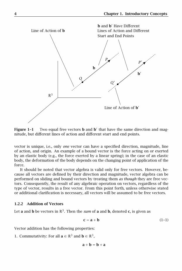
A free vector is any vector b with no specified line of action or point of applicationin R3. Figure 1–1 shows an example of two identical free vectors b and b′. While band b′ have the same direction and magnitude, they do not share the same start orend point. In particular, b starts at point Q and ends at point P while b′ starts atpoint Q′ ≠ Q and ends at point P ′ ≠ P . However, because b and b′ have the samedirection and magnitude, they are identical free vectors. Examples of free vectors arethe angular velocity of a reference frame or a rigid body, a pure torque applied to arigid body, and a basis vector.
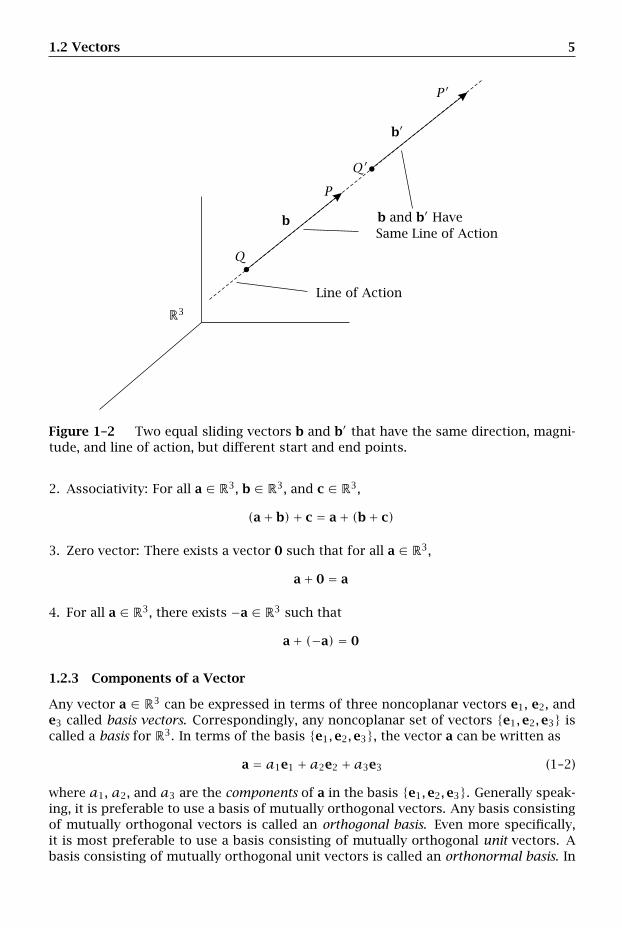
A sliding vector is any vector b that has a specified line of action or axis in R3,but has no specified point of application in R3. Figure 1–2 shows two identical slidingvectors b and b′. As with free vectors, b and b′ have the same magnitude and direction.However, while the vector b starts at pointQ and ends at point P , the vector b′ starts atpoint Q′ ≠ Q and ends at point P ′ ≠ P (where the points P , Q, P ′, and Q′ are colinear).Consequently, b and b′ are identical sliding vectors, but are different free vectors. Anexample of a sliding vector is the force applied to a rigid body.
A bound vector is any vector that has both a specified line of action in R3 and aspecified point of application in R3. From its definition, it can be seen that a bound
1An excellent description of free, sliding, and bound vectors can be found in either Synge and Griffith(1959) or Greenwood (1988).
4 Chapter 1. Introductory Concepts
b
P
Qb′
P ′
Q′
Line of Action of b
Line of Action of b′
b and b′ Have DifferentLines of Action and DifferentStart and End Points
R3
Figure 1–1 Two equal free vectors b and b′ that have the same direction and mag-nitude, but different lines of action and different start and end points.
vector is unique, i.e., only one vector can have a specified direction, magnitude, lineof action, and origin. An example of a bound vector is the force acting on or exertedby an elastic body (e.g., the force exerted by a linear spring); in the case of an elasticbody, the deformation of the body depends on the changing point of application of theforce.
It should be noted that vector algebra is valid only for free vectors. However, be-cause all vectors are defined by their direction and magnitude, vector algebra can beperformed on sliding and bound vectors by treating them as though they are free vec-tors. Consequently, the result of any algebraic operation on vectors, regardless of thetype of vector, results in a free vector. From this point forth, unless otherwise statedor additional clarification is necessary, all vectors will be assumed to be free vectors.
1.2.2 Addition of Vectors
Let a and b be vectors in R3. Then the sum of a and b, denoted c, is given as
c = a+ b (1–1)
Vector addition has the following properties:
1. Commutativity: For all a ∈ R3 and b ∈ R3,
a+ b = b+ a
1.2 Vectors 5
b
P
Q
b′
P ′
Q′
b and b′ Have
Line of Action
Same Line of Action
R3
Figure 1–2 Two equal sliding vectors b and b′ that have the same direction, magni-tude, and line of action, but different start and end points.
2. Associativity: For all a ∈ R3, b ∈ R3, and c ∈ R3,
(a+ b)+ c = a+ (b+ c)
3. Zero vector: There exists a vector 0 such that for all a ∈ R3,
a+ 0 = a
4. For all a ∈ R3, there exists −a ∈ R3 such that
a+ (−a) = 0
1.2.3 Components of a Vector
Any vector a ∈ R3 can be expressed in terms of three noncoplanar vectors e1, e2, ande3 called basis vectors. Correspondingly, any noncoplanar set of vectors e1,e2,e3 iscalled a basis for R3. In terms of the basis e1,e2,e3, the vector a can be written as
a = a1e1 + a2e2 + a3e3 (1–2)
where a1, a2, and a3 are the components of a in the basis e1,e2,e3. Generally speak-ing, it is preferable to use a basis of mutually orthogonal vectors. Any basis consistingof mutually orthogonal vectors is called an orthogonal basis. Even more specifically,it is most preferable to use a basis consisting of mutually orthogonal unit vectors. Abasis consisting of mutually orthogonal unit vectors is called an orthonormal basis. In
6 Chapter 1. Introductory Concepts
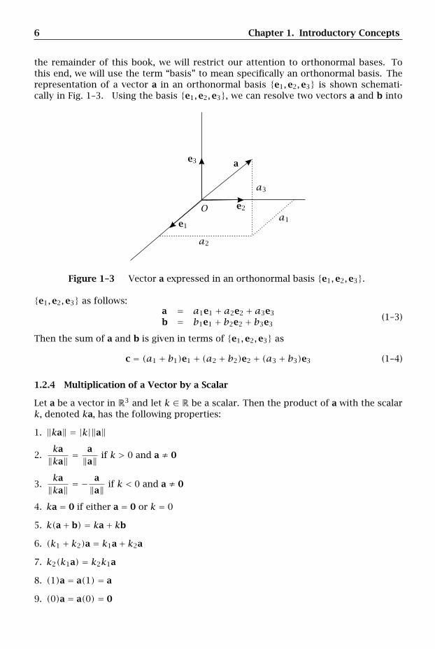
the remainder of this book, we will restrict our attention to orthonormal bases. Tothis end, we will use the term “basis” to mean specifically an orthonormal basis. Therepresentation of a vector a in an orthonormal basis e1,e2,e3 is shown schemati-cally in Fig. 1–3. Using the basis e1,e2,e3, we can resolve two vectors a and b into
a1
a2
a3
e1
e2
e3 a
O
Figure 1–3 Vector a expressed in an orthonormal basis e1,e2,e3.
e1,e2,e3 as follows:a = a1e1 + a2e2 + a3e3
b = b1e1 + b2e2 + b3e3(1–3)
Then the sum of a and b is given in terms of e1,e2,e3 as
c = (a1 + b1)e1 + (a2 + b2)e2 + (a3 + b3)e3 (1–4)
1.2.4 Multiplication of a Vector by a Scalar
Let a be a vector in R3 and let k ∈ R be a scalar. Then the product of a with the scalark, denoted ka, has the following properties:
1. ‖ka‖ = |k|‖a‖
2.ka‖ka‖ =
a‖a‖ if k > 0 and a ≠ 0
3.ka‖ka‖ = −
a‖a‖ if k < 0 and a ≠ 0
4. ka = 0 if either a = 0 or k = 0
5. k(a+ b) = ka+ kb
6. (k1 + k2)a = k1a+ k2a
7. k2(k1a) = k2k1a
8. (1)a = a(1) = a
9. (0)a = a(0) = 0
1.2 Vectors 7
10. (−1)a = a(−1) = −a
Finally, if a is expressed in the basis e1,e2,e3, then ka is given as
ka = ka1e1 + ka2e2 + ka3e3 (1–5)
1.2.5 Scalar Product
Let a and b be vectors in R3. Then the scalar product or dot product between a and bis defined as
a · b = ‖a‖‖b‖ cosθ = ab cosθ (1–6)
where θ is the angle between a and b. The scalar product has the following properties:
1. a · b = b · a
2. a · (kb) = ka · b where k ∈ R3. (a+ b) · c = a · c+ b · c
Two nonzero vectors are said to be orthogonal if their scalar product is zero, i.e., a andb are orthogonal if
a · b = 0 (a,b ≠ 0) (1–7)
A set of vectors a1, . . . ,an is said to be mutually orthogonal if
ai · aj = 0 (i ≠ j, i, j = 1, . . . , n) (1–8)
Finally, the magnitude of a vector a is equal to the square root of the dot product ofthe vector with itself, i.e.,
‖a‖ = √a · a (1–9)
Suppose now that a and b are expressed in a particular basis e1,e2,e3 as
a = a1e1 + a2e2 + a3e3
b = b1e1 + b2e2 + b3e3(1–10)
Then the scalar product of a with b is given as
a · b = (a1e1 + a2e2 + a3e3) · (b1e1 + b2e2 + b3e3) (1–11)
Because we are restricting attention to orthonormal bases, the basis e1,e2,e3 satis-fies the properties that
ei · ej =
1 (i = j)0 (i ≠ j) (i, j = 1,2,3) (1–12)
Consequently, we havea · b = a1b1 + a2b2 + a3b3 (1–13)
Using Eq. (1–13) and the definition of the magnitude of a vector as given in Eq. (1–9),the magnitude of a vector a can be written in terms of the components of a in the basise1,e2,e3 as
‖a‖ =√a2
1 + a22 + a2
3 (1–14)
8 Chapter 1. Introductory Concepts
1.2.6 Vector Product
Let a and b be vectors in R3. Then the vector product or cross product between twovectors a and b is defined as
c = a× b = ‖a‖‖b‖ sinθn (1–15)
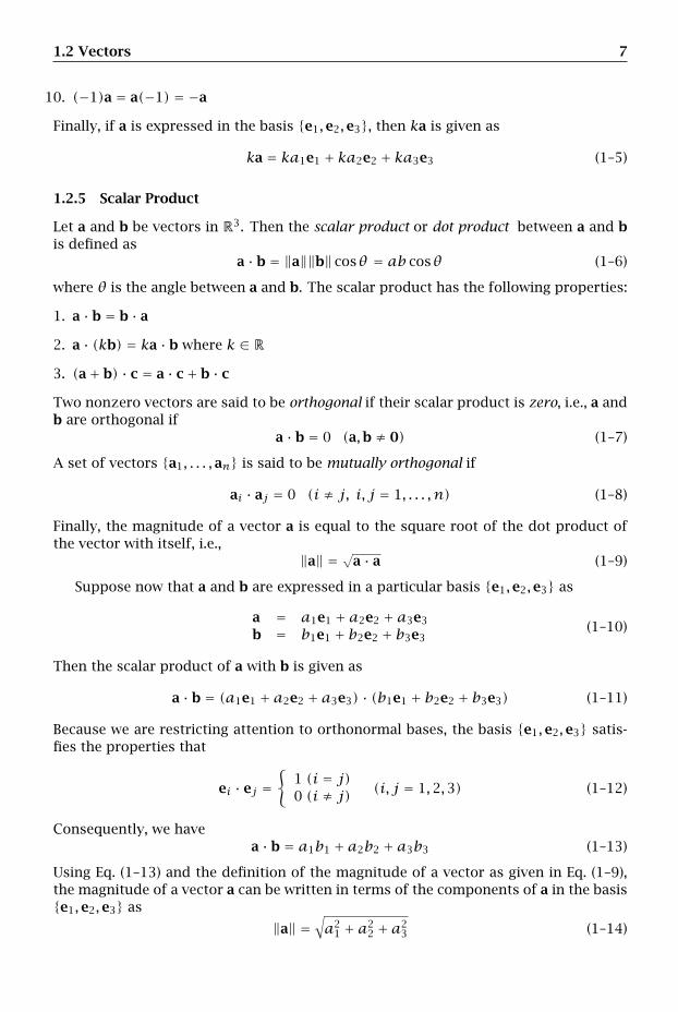
where n is the unit vector in the direction orthogonal to both a and b in a right-handedsense and θ is the angle between a and b. The term “right-handed sense” arises fromthe fact that the vectors a, b, and c assume an orientation that corresponds to theindex finger, middle finger, and thumb of the right hand when these three fingers areheld as shown in Fig. 1–4.
a
b
c
n
Figure 1–4 Schematic of right-hand rule corresponding to the vector product of twovectors using the index finger, middle finger, and thumb of the right hand.
The magnitude of the vector product of two vectors is given as
‖c‖ = ‖a‖‖b‖ sinθ (1–16)
The vector product has the following properties:
1. a× a = 0
2. a× b = −b× a
3. (ka)× b = k(a× b) = a× (kb) where k ∈ R4. (a+ b)× c = (a× c)+ (b× c)
Now suppose that a and b are expressed in terms of the basis e1,e2,e3, i.e.,
a = a1e1 + a2e2 + a3e3
b = b1e1 + b2e2 + b3e3(1–17)
1.2 Vectors 9
Then the cross product of a and b is given as
a× b = (a1e1 + a2e2 + a3e3)× (b1e1 + b2e2 + b3e3) (1–18)
Expanding Eq. (1–18), we obtain
a× b = a1b2e1 × e2 + a1b3e1 × e3 + a2b1e2 × e1
+ a2b3e2 × e3 + a3b1e3 × e1 + a3b2e3 × e2(1–19)
Again we remind the reader that we are restricting our attention to orthonormal bases.Furthermore, suppose that the basis e1,e2,e3 forms a right-handed set, i.e., e1,e2,e3satisfies the following properties:
e1 × e2 = e3
e2 × e3 = e1
e3 × e1 = e2
(1–20)
Then a× b is given as
a× b = (a2b3 − a3b2)e1 + (a3b1 − a1b3)e2 + (a1b2 − a2b1)e3 (1–21)
In terms of a right-handed basis, Eq. (1–21) can also be written as the following deter-minant (Kreyszig, 1988):
a× b =
∣∣∣∣∣∣∣e1 e2 e3
a1 a2 a3
b1 b2 b3
∣∣∣∣∣∣∣ (1–22)
1.2.7 Scalar Triple Product
Given three vectors a, b, and c, the scalar triple product is defined as
a · (b× c) (1–23)
The scalar triple product has the following properties:
1. a · (b× c) = (a× b) · c = b · (c× a) = c · (a× b)
2. a · (kb× c) = ka · (b× c)
Suppose that the vectors a, b, and c are each expressed in an orthonormal basise1,e2,e3 as
a = a1e1 + a2e2 + a3e3
b = b1e1 + b2e2 + b3e3
c = c1e1 + c2e2 + c3e3
(1–24)
Then the scalar triple product can be written as
a · (b× c) = a1(b2c3 − b3c2)+ a2(b3c1 − b1c3)+ a3(b1c2 − b2c1) (1–25)
The scalar triple product can also be written as the following determinant:
a · (b× c) =
∣∣∣∣∣∣∣a1 a2 a3
b1 b2 b3
c1 c2 c3
∣∣∣∣∣∣∣ (1–26)
Finally, the scalar triple product can be written as
a · (b× c) = ‖a‖‖b× c‖ cosθ (1–27)
where θ is the angle between the vector a and the vector b× c.
10 Chapter 1. Introductory Concepts
1.2.8 Vector Triple Product
Given three vectors a, b, and c, the vector triple product is given as
a× (b× c) (1–28)
The vector triple product can be written as
a× (b× c) = (a · c)b− (a · b)c (1–29)
Suppose that the vectors a, b, and c are each expressed in an orthonormal basise1,e2,e3 as
a = a1e1 + a2e2 + a3e3
b = b1e1 + b2e2 + b3e3
c = c1e1 + c2e2 + c3e3
(1–30)
The vector triple product can then be written as
a× (b× c) = (a1c1 + a2c2 + a3c3)(b1e1 + b2e2 + b3e3)− (a1b1 + a2b2 + a3b3)(c1e1 + c2e2 + c3e3)
(1–31)
1.3 Tensors
A tensor (or second-order tensor2), denoted T, is a linear operator that associates avector a ∈ R3 to another vector b ∈ R3, i.e., if T is a tensor and a ∈ R3 is a vector, thenthere exists a vector b such that
b = T · a (1–32)
It is noted that the binary operator “·” in Eq. (1–32) is different from the scalar productbetween two vectors in that the “·” denotes the operation of the tensor T on the vectora. Now, because tensors are linear operators, they satisfy the following properties:
1. For all a,b ∈ R3,T · (a+ b) = T · a+ T · b
2. For all a ∈ R3 and k ∈ R,T · (ka) = kT · a
3. There exists a zero tensor, denoted O, such that for every a ∈ R3,
O · a = 0 (1–33)
where 0 is the zero vector.
4. There exists an identity tensor or unit tensor, denoted U, such that for every a ∈ R3,
U · a = a (1–34)
2Strictly speaking, the tensor defined in Eq. (1–32) is a second-order tensor. While tensor algebra gener-alizes well beyond second-order tensors, in this book we will only be concerned with second-order tensors.Consequently, throughout this book we will use the term “tensor” to mean “second-order tensor”.
1.3 Tensors 11
1.3.1 Important Classes of Tensors
A tensor T is said to be invertible if there exists a tensor T−1 such that
T · T−1 = T−1 · T = U (1–35)
If T is invertible, then T−1 is called the inverse of T. The transpose of a tensor T,denoted TT , satisfies the property that for all a ∈ R3 and b ∈ R3,
(TT · a) · b = a · (T · b) (1–36)
A tensor T is said to be symmetric if it is equal to its transpose, i.e., T is symmetric if
T = TT (1–37)
A tensor T is said to be skew-symmetric if it is equal to the negative of its transpose,i.e., T is skew-symmetric if
T = −TT (1–38)
Finally, an invertible tensor T is said to be orthogonal if its transpose is equal to itsinverse, i.e., T is orthogonal if
TT = T−1 (1–39)
1.3.2 Tensor Product Between Vectors
Let a and b be vectors in R3. Then the tensor product of a and b, denoted a ⊗ b, isdefined as
T = a⊗ b (1–40)
where T is the tensor that results from the tensor product between a and b. It canbe seen that a tensor is obtained from an operation on a pair of vectors. Then, usingEq. (1–32), the scalar product between the tensor a⊗ b and the vector c is defined as
(a⊗ b) · c ≡ (b · c)a (1–41)
c · (a⊗ b) ≡ (a · c)b (1–42)
It can be seen that, unlike the scalar product between two vectors, the scalar productbetween a tensor a ⊗ b and a vector c depends on the order of the operation, i.e., ingeneral we have that
(a⊗ b) · c ≠ c · (a⊗ b) (1–43)
Suppose now that we let e1,e2,e3 be an orthonormal basis for R3. Then, usingEq. (1–41), we have
(ei ⊗ ej) · ek = (ej · ek)ei (i, j, k = 1,2,3) (1–44)
Substituting the expression for ei ⊗ ej from Eq. (1–12) into Eq. (1–44), we obtain
ei ⊗ ej · ek =
ei (j = k)0 (j ≠ k) (i, j, k = 1,2,3) (1–45)

12 Chapter 1. Introductory Concepts
1.3.3 Basis Representations of Tensors
Suppose now that we let a ∈ R3 and b ∈ R3. Then a and b can be expressed in theorthonormal basis e1,e2,e3 as
a = a1e1 + a2e2 + a3e3
b = b1e1 + b2e2 + b3e3(1–46)
The tensor product between a and b is then given as
a⊗ b = (a1e1 + a2e2 + a3e3)⊗ (b1e1 + b2e2 + b3e3) (1–47)
Expanding Eq. (1–47) term-by-term, we have
a⊗ b =3∑i=1
3∑j=1
aibjei ⊗ ej (1–48)
Now, because a⊗b is a tensor, it is seen from Eq. (1–48) that a tensor T can be expressedin an orthonormal basis e1,e2,e3 as
T =3∑i=1
3∑j=1
Tijei ⊗ ej (1–49)
Eq. (1–49) is called the representation of the tensor T in the basis e1,e2,e3. UsingEq. (1–49), the transpose of T is obtained from T as
TT =3∑i=1
3∑j=1
Tijej ⊗ ei (1–50)
In particular, it is seen that the representation of TT is obtained from the representa-tion of T by interchanging the order of the tensor products ei⊗ ej (i, j = 1,2,3). Now,in terms of the basis e1,e2,e3, the identity tensor U is given as
U =3∑i=1
3∑j=1
Uijei ⊗ ej =3∑i=1
ei ⊗ ei (1–51)
In other words, for the identity tensor, we have
Uij =
1 if i = j0 if i ≠ j (1–52)
Example 1–1
Show that the vector triple product a× (b× c) can be written in the tensor form
a× (b× c) = (b⊗ a) · c− (c⊗ a) · b
1.3 Tensors 13
Solution to Example 1–1
Recall from Eq. (1–29) that the vector triple product is given as
a× (b× c) = (a · c)b− (a · b)c (1–53)
Then, using the property of the tensor product as given in Eq. (1–41), we have
(a · c)b = (b⊗ a) · c (1–54)
(a · b)c = (c⊗ a) · b (1–55)
Finally, substituting the results from Eqs. (1–54) and (1–55) into Eq. (1–53), we obtain
a× (b× c) = (b⊗ a) · c− (c⊗ a) · b (1–56)
Example 1–2
Given two vectors a and b expressed in the orthonormal basis e1,e2,e3, show thatthe vector product a× b can be written as T · b, where T is the tensor
T = −a3e1 ⊗ e2 + a2e1 ⊗ e3
+ a3e2 ⊗ e1 − a1e2 ⊗ e3
− a2e3 ⊗ e1 + a1e3 ⊗ e2
Solution to Example 1–2
In terms of the basis, the product of the tensor T with the vector b is given as
T · b = (−a3e1 ⊗ e2 + a2e1 ⊗ e3 + a3e2 ⊗ e1 − a1e2 ⊗ e3
−a2e3 ⊗ e1 + a1e3 ⊗ e2) · (b1e1 + b2e2 + b3e3)(1–57)
Then, expanding Eq. (1–57) using Eq. (1–45) on each term, we have
T · b = a3b1e2 − a2b1e3 − a3b2e1 + a1b2e3 + a2b3e1 − a1b3e2 (1–58)
Grouping terms in Eq. (1–58), we obtain
T · b = (a2b3 − a3b2)e1 + (a3b1 − a1b3)e2 + (a1b2 − a2b1)e3 (1–59)
It can be seen that Eq. (1–59) is identical to Eq. (1–21), i.e., we have
T · b ≡ a× b (1–60)
which implies that the tensor T is equivalent to the operator “a×,” i.e.,
T ≡ a× (1–61)
14 Chapter 1. Introductory Concepts
1.4 Matrices
1.4.1 Systems of Linear Equations
Consider a system of equations of the form
a11x1 + a12x2 + · · ·a1nxn = b1
a21x1 + a22x2 + · · ·a2nxn = b2...
an1x1 + an2x2 + · · ·annxn = bn
(1–62)
where aij (i, j = 1, . . . , n) and bi (i = 1, . . . , n) are known and xi (i = 1, . . . , n) areunknown. Equation (1–62) is called a system of n linear equations in the n unknownsxi (i = 1, . . . , n). This system can be written in matrix form as⎧⎪⎪⎪⎪⎨
⎪⎪⎪⎪⎩
a11 · · · a1na21 · · · a2n
...an1 · · · ann
⎫⎪⎪⎪⎪⎬⎪⎪⎪⎪⎭
⎧⎪⎪⎪⎪⎨⎪⎪⎪⎪⎩
x1
x2...xn
⎫⎪⎪⎪⎪⎬⎪⎪⎪⎪⎭=
⎧⎪⎪⎪⎪⎨⎪⎪⎪⎪⎩
b1
b2...bn
⎫⎪⎪⎪⎪⎬⎪⎪⎪⎪⎭
(1–63)
Suppose now that we make the following substitutions:
A =
⎧⎪⎪⎪⎪⎨⎪⎪⎪⎪⎩
a11 · · · a1na21 · · · a2n
...an1 · · · ann
⎫⎪⎪⎪⎪⎬⎪⎪⎪⎪⎭
(1–64)
x =
⎧⎪⎪⎪⎪⎨⎪⎪⎪⎪⎩
x1
x2...xn
⎫⎪⎪⎪⎪⎬⎪⎪⎪⎪⎭
(1–65)
b =
⎧⎪⎪⎪⎪⎨⎪⎪⎪⎪⎩
b1
b2...bn
⎫⎪⎪⎪⎪⎬⎪⎪⎪⎪⎭
(1–66)
Then Eq. (1–63) can be written compactly as
Ax = b (1–67)
The quantity A ∈ Rn×n is called a matrix while the quantities x ∈ Rn and b ∈ Rn arecalled column-vectors.
1.4.2 Classes of Matrices
Suppose we are given a matrix A ∈ Rn×n defined as
A =
⎧⎪⎪⎪⎪⎨⎪⎪⎪⎪⎩
a11 · · · a1na21 · · · a2n
...an1 · · · ann
⎫⎪⎪⎪⎪⎬⎪⎪⎪⎪⎭
(1–68)
1.4 Matrices 15
Then A is said to be invertible if there exists a matrix A−1 such that
AA−1 = A−1A = I (1–69)
where
I =
⎧⎪⎪⎪⎪⎨⎪⎪⎪⎪⎩
1 0 0 · · · 00 1 0 · · · 0...
......
......
0 0 0 · · · 1
⎫⎪⎪⎪⎪⎬⎪⎪⎪⎪⎭
(1–70)
is the n × n identity matrix. If A is invertible, the A−1 is called the inverse of A. Thetranspose of a matrix A, denoted AT , is defined as
AT =
⎧⎪⎪⎪⎪⎨⎪⎪⎪⎪⎩
a11 · · · an1
a12 · · · an2...
a1n · · · ann
⎫⎪⎪⎪⎪⎬⎪⎪⎪⎪⎭
(1–71)
It can be seen that the matrix transpose is obtained by interchanging the rows and thecolumns in the matrix A. Using the definition of the transpose of a matrix, a row-vectoris defined as the transpose of a column-vector, i.e., if x is the column-vector
x =
⎧⎪⎪⎪⎪⎨⎪⎪⎪⎪⎩
x1
x2...xn
⎫⎪⎪⎪⎪⎬⎪⎪⎪⎪⎭
(1–72)
thenxT =
x1 x2 · · · xn
(1–73)
is a row-vector. A matrix is said to be symmetric if
A = AT (1–74)
A matrix A is said to be skew-symmetric if
A = −AT (1–75)
Finally, an invertible matrix is said to be orthogonal if
AT = A−1 (1–76)
1.4.3 Relationship Between Tensors and Matrices
Consider the equationT · x = b (1–77)
where T ∈ R3×3 is a tensor and x ∈ R3 and b ∈ R3 are vectors. Suppose now thatwe choose to express each of the quantities in Eq. (1–77) in terms of an arbitrary
16 Chapter 1. Introductory Concepts
orthonormal basis e1,e2,e3 as
T =3∑i=1
3∑j=1
Tijei ⊗ ej
x = ∑3i=1 xiei
b = ∑3i=1 biei
(1–78)
Substituting the expressions from Eq. (1–78) into Eq. (1–77), we have⎡⎣ 3∑i=1
3∑j=1
Tijei ⊗ ej
⎤⎦ ·
⎡⎣ 3∑i=1
xiei
⎤⎦ = 3∑
i=1
biei (1–79)
Then, using the property of Eq. (1–45) in Eq. (1–79), we obtain
3∑i=1
3∑j=1
Tijxjei =3∑i=1
biei (1–80)
Equation (1–80) can be written in matrix form as⎧⎪⎨⎪⎩T11 T12 T13
T21 T22 T23
T31 T32 T33
⎫⎪⎬⎪⎭⎧⎪⎨⎪⎩x1
x2
x3
⎫⎪⎬⎪⎭ =
⎧⎪⎨⎪⎩b1
b2
b3
⎫⎪⎬⎪⎭ (1–81)
More compactly, Eq. (1–81) can be written as
TE xE = bE (1–82)
where
TE =
⎧⎪⎨⎪⎩T11 T12 T13
T21 T22 T23
T31 T32 T33
⎫⎪⎬⎪⎭ (1–83)
is called the matrix representation of the tensor in the basis E = e1,e2,e3 while thequantities
xE =
⎧⎪⎨⎪⎩x1
x2
x3
⎫⎪⎬⎪⎭ (1–84)
and
bE =
⎧⎪⎨⎪⎩b1
b2
b3
⎫⎪⎬⎪⎭ (1–85)
are called the column-vector representations of the vectors x and b in the basis E.The previous discussion shows the relationship between tensors and matrices. In
particular, Eq. (1–81) shows that a column-vector is not a vector. Furthermore, Eq. (1–81) shows that a matrix is not a tensor. Instead, a column-vector and a matrix arerepresentations of a vector and a tensor, respectively, in a particular basis. Conse-quently, both a column-vector and a matrix are specific to a particular basis, whereasvectors and tensors are independent of any particular basis.
1.4 Matrices 17
Another way of viewing the relationships between vector and column-vectors andtensors and matrices is as follows. Suppose that a basis U = u1,u2,u3 is chosen thatis different from the basis e1,e2,e3. Then the column-vector representations of thevectors x and b and the matrix representation of the tensor T in the basis u1,u2,u3will be different from their respective representations in the basis e1,e2,e3. Mathe-matically, if E = e1,e2,e3 and U = u1,u2,u3 are distinct bases, then
TE ≠ TU
xE ≠ xU
bE ≠ bU
(1–86)
Now, while the matrix representation of a tensor or the column-vector representationof a vector is different in different bases, the underlying tensor or vector itself is thesame regardless of the basis. In other words, a tensor and a vector are coordinate-freequantities while the matrix representation of a tensor or the column-vector represen-tation of a vector depends on the particular coordinate system (i.e., basis) in which thetensor or vector is expressed.
Example 1–3
Given two vectors a and b and an orthonormal basis E, show that the scalar product ofa with b is equal to the product of the transpose of the column-vector representationof a with the column-vector representation of b, i.e., show that
a · b = aTE bE
Solution to Example 1–3
The vectors a and b can be decomposed in the basis E = e1,e2,e3 as
a = a1e1 + a2e2 + a3e3 (1–87)
b = b1e1 + b2e2 + b3e3 (1–88)
Then the scalar of a with b is given as
a · b = a1b1 + a2b2 + a3b3 (1–89)
Furthermore, the column-vector representations of a and b in the basis E are given,respectively, as
aE =
⎧⎪⎨⎪⎩a1
a2
a3
⎫⎪⎬⎪⎭ (1–90)
bE =
⎧⎪⎨⎪⎩b1
b2
b3
⎫⎪⎬⎪⎭ (1–91)
Consequently, we have
a1b1 + a2b2 + a3b3 =a1 a2 a3
⎧⎪⎨⎪⎩b1
b2
b3
⎫⎪⎬⎪⎭ (1–92)
18 Chapter 1. Introductory Concepts
Furthermore, the transpose of aE is given as
aTE =a1 a2 a3
(1–93)
Therefore, the scalar product of a with b in the basis E is given as
a · b = aTE bE (1–94)
Example 1–4
Given two vectors a and b expressed in the orthonormal basis E = e1,e2,e3, deter-mine the matrix representation of the tensor product a⊗b in the basis E, i.e., determine
a⊗ bE
Solution to Example 1–4
The vectors a and b can be decomposed in the basis E = e1,e2,e3 as
a = a1e1 + a2e2 + a3e3 (1–95)
b = b1e1 + b2e2 + b3e3 (1–96)
Then, the tensor product between a and b is given as
a⊗ b = (a1e1 + a2e2 + a3e3)⊗ (b1e1 + b2e2 + b3e3) =3∑i=1
3∑j=1
aibjei ⊗ ej (1–97)
Finally, extracting the coefficients of the tensor a⊗b in Eq. (1–97), the matrix represen-tation of a⊗ b in the basis E is given as
a⊗ bE =
⎧⎪⎨⎪⎩a1b1 a1b2 a1b3
a2b1 a2b2 a2b3
a3b1 a3b2 a3b3
⎫⎪⎬⎪⎭ (1–98)
Example 1–5
Determine the matrix representation of the tensor T from Example 1–2.
1.4 Matrices 19
Solution to Example 1–5
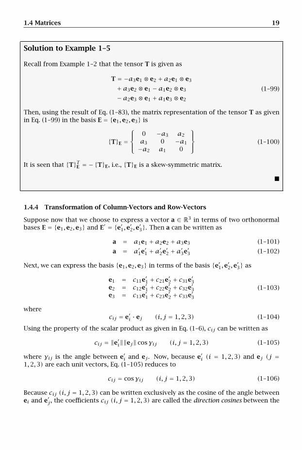
Recall from Example 1–2 that the tensor T is given as
T = −a3e1 ⊗ e2 + a2e1 ⊗ e3
+ a3e2 ⊗ e1 − a1e2 ⊗ e3
− a2e3 ⊗ e1 + a1e3 ⊗ e2
(1–99)
Then, using the result of Eq. (1–83), the matrix representation of the tensor T as givenin Eq. (1–99) in the basis E = e1,e2,e3 is
TE =
⎧⎪⎨⎪⎩
0 −a3 a2
a3 0 −a1
−a2 a1 0
⎫⎪⎬⎪⎭ (1–100)
It is seen that TTE = −TE, i.e., TE is a skew-symmetric matrix.
1.4.4 Transformation of Column-Vectors and Row-Vectors
Suppose now that we choose to express a vector a ∈ R3 in terms of two orthonormalbases E = e1,e2,e3 and E′ = e′1,e′2,e′3. Then a can be written as
a = a1e1 + a2e2 + a3e3 (1–101)
a = a′1e′1 + a′2e′2 + a′3e′3 (1–102)
Next, we can express the basis e1,e2,e3 in terms of the basis e′1,e′2,e′3 as
e1 = c11e′1 + c21e′2 + c31e′3e2 = c12e′1 + c22e′2 + c32e′3e3 = c13e′1 + c23e′2 + c33e′3
(1–103)
wherecij = e′i · ej (i, j = 1,2,3) (1–104)
Using the property of the scalar product as given in Eq. (1–6), cij can be written as
cij = ‖e′i‖‖ej‖ cosγij (i, j = 1,2,3) (1–105)
where γij is the angle between e′i and ej . Now, because e′i (i = 1,2,3) and ej (j =1,2,3) are each unit vectors, Eq. (1–105) reduces to
cij = cosγij (i, j = 1,2,3) (1–106)
Because cij (i, j = 1,2,3) can be written exclusively as the cosine of the angle betweenei and e′j , the coefficients cij (i, j = 1,2,3) are called the direction cosines between the

20 Chapter 1. Introductory Concepts
basis vectors in E and the basis vectors in E′. Substituting the results of Eq. (1–103)into Eq. (1–101), we obtain
a = a1(c11e′1 + c21e′2 + c31e′3)+ a2(c12e′1 + c22e′2 + c32e′3)+ a3(c13e′1 + c23e′2 + c33e′3)
(1–107)
Rearranging Eq. (1–107), we obtain
a = (c11a1 + c12a2 + c13a3)e′1+ (c21a1 + c22a2 + c23a3)e′2+ (c31a1 + c32a2 + c33a3)e′3
(1–108)
Then, setting the expression for a from Eq. (1–108) equal to the expression for a fromEq. (1–102), we obtain
a′1 = c11a1 + c12a2 + c13a3
a′2 = c21a1 + c22a2 + c23a3
a′3 = c31a1 + c32a2 + c33a3
(1–109)
Using matrix notation, we can write Eq. (1–109) as⎧⎪⎨⎪⎩a′1a′2a′3
⎫⎪⎬⎪⎭ =
⎧⎪⎨⎪⎩c11 c12 c13
c21 c22 c23
c31 c32 c33
⎫⎪⎬⎪⎭⎧⎪⎨⎪⎩a1
a2
a3
⎫⎪⎬⎪⎭ (1–110)
Now we see that the coefficient matrix transforms column-vectors from the basis E tothe basis E′. In order to specify the direction of the transformation unambiguously, weuse the following notation:
CE′E =
⎧⎪⎨⎪⎩c11 c12 c13
c21 c22 c23
c31 c32 c33
⎫⎪⎬⎪⎭ (1–111)
where the right subscript denotes the basis from which the transformation is per-formed while the right superscript denotes the basis to which the transformation isperformed. In other words, the quantity CE′
E is the matrix that transforms column-vectors from the basis E to the basis E′. The matrix CE′
E is called the direction cosinematrix from the basis E to the basis E′. In terms of the direction cosine matrix, we canwrite Eq. (1–110) compactly as
aE′ = CE′E aE (1–112)
where aE and aE′ are the column-vector representations of the vector a in the basesE and E′, respectively. Equation (1–112) provides a way to transform the componentsof a vector from the basis E = e1,e2,e3 to the basis E′ = e′1,e′2,e′3. Equivalently,the direction cosine tensor C is given as
C =3∑i=1
3∑j=1
cije′i ⊗ ej (1–113)
It should be noted that the tensor C of Eq. (1–113) is expressed as the sum of the tensorproducts formed by basis vectors in both the basis E and the basis E′.
1.4 Matrices 21
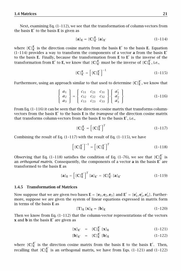
Next, examining Eq. (1–112), we see that the transformation of column-vectors fromthe basis E′ to the basis E is given as
aE = CEE′ aE′ (1–114)
where CEE′ is the direction cosine matrix from the basis E′ to the basis E. Equation
(1–114) provides a way to transform the components of a vector a from the basis E′
to the basis E. Finally, because the transformation from E to E′ is the inverse of thetransformation from E′ to E, we know that CE
E′ must be the inverse of CE′E , i.e.,
CEE′ =
[CE′
E
]−1(1–115)
Furthermore, using an approach similar to that used to determine CE′E , we know that⎧⎪⎨
⎪⎩a1
a2
a3
⎫⎪⎬⎪⎭ =
⎧⎪⎨⎪⎩c11 c21 c31
c12 c22 c32
c13 c23 c33
⎫⎪⎬⎪⎭⎧⎪⎨⎪⎩a′1a′2a′3
⎫⎪⎬⎪⎭ (1–116)
From Eq. (1–116) it can be seen that the direction cosine matrix that transforms column-vectors from the basis E′ to the basis E is the transpose of the direction cosine matrixthat transforms column-vectors from the basis E to the basis E′, i.e.,
CEE′ =
[CE′
E
]T(1–117)
Combining the result of Eq. (1–117) with the result of Eq. (1–115), we have
[CE′
E
]−1 =[CE′
E
]T(1–118)
Observing that Eq. (1–118) satisfies the condition of Eq. (1–76), we see that CE′E is
an orthogonal matrix. Consequently, the components of a vector a in the basis E′ aretransformed to the basis E as
aE =[CE′
E
]T aE′ = CEE′ aE′ (1–119)
1.4.5 Transformation of Matrices
Now suppose that we are given two bases E = e1,e2,e3 and E′ = e′1,e′2,e′3. Further-more, suppose we are given the system of linear equations expressed in matrix formin terms of the basis E as
TE xE = bE (1–120)
Then we know from Eq. (1–112) that the column-vector representations of the vectorsx and b in the basis E′ are given as
xE′ = CE′E xE (1–121)
bE′ = CE′E bE (1–122)
where CE′E is the direction cosine matrix from the basis E to the basis E′. Then,
recalling that CE′E is an orthogonal matrix, we have from Eqs. (1–121) and (1–122)
22 Chapter 1. Introductory Concepts
that
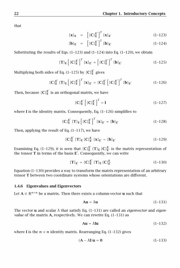
xE =[CE′
E
]T xE′ (1–123)
bE =[CE′
E
]T bE′ (1–124)
Substituting the results of Eqs. (1–123) and (1–124) into Eq. (1–120), we obtain
TE
[CE′
E
]T xE′ =[CE′
E
]T bE′ (1–125)
Multiplying both sides of Eq. (1–125) by CE′E gives
CE′E TE
[CE′
E
]T xE′ = CE′E
[CE′
E
]T bE′ (1–126)
Then, because CE′E is an orthogonal matrix, we have
CE′E
[CE′
E
]T = I (1–127)
where I is the identity matrix. Consequently, Eq. (1–126) simplifies to
CE′E TE
[CE′
E
]T xE′ = bE′ (1–128)
Then, applying the result of Eq. (1–117), we have
CE′E TE CE
E′ xE′ = bE′ (1–129)
Examining Eq. (1–129), it is seen that CE′E TE CE
E′ is the matrix representation ofthe tensor T in terms of the basis E′. Consequently, we can write
TE′ = CE′E TE CE
E′ (1–130)
Equation (1–130) provides a way to transform the matrix representation of an arbitrarytensor T between two coordinate systems whose orientations are different.
1.4.6 Eigenvalues and Eigenvectors
Let A ∈ Rn×n be a matrix. Then there exists a column-vector u such that
Au = λu (1–131)
The vector u and scalar λ that satisfy Eq. (1–131) are called an eigenvector and eigen-value of the matrix A, respectively. We can rewrite Eq. (1–131) as
Au = λIu (1–132)
where I is the n×n identity matrix. Rearranging Eq. (1–132) gives
(A− λI)u = 0 (1–133)
1.4 Matrices 23
Then, using the general expression for an n×n matrix and an n-dimensional column-vector as given in Eq. (1–63), we can write Eq. (1–133) in expanded form as⎧⎪⎪⎪⎪⎪⎨
⎪⎪⎪⎪⎪⎩
a11 − λ a12 · · · a1na21 a22 − λ · · · a2n
......
an1 an2... ann − λ
⎫⎪⎪⎪⎪⎪⎬⎪⎪⎪⎪⎪⎭
⎧⎪⎪⎪⎪⎨⎪⎪⎪⎪⎩
u1
u2...un
⎫⎪⎪⎪⎪⎬⎪⎪⎪⎪⎭=
⎧⎪⎪⎪⎪⎨⎪⎪⎪⎪⎩
00...0
⎫⎪⎪⎪⎪⎬⎪⎪⎪⎪⎭
(1–134)
Now, it is well known that the solution of Eq. (1–134) is obtained by solving for thosevalues of λ that are the roots of the so-called characteristic equation:
det(A− λI) = det
⎧⎪⎪⎪⎪⎪⎨⎪⎪⎪⎪⎪⎩
a11 − λ a12 · · · a1na21 a22 − λ · · · a2n
......
an1 an2... ann − λ
⎫⎪⎪⎪⎪⎪⎬⎪⎪⎪⎪⎪⎭= 0 (1–135)
where det(·) is the determinant function (Kreyszig, 1988). Because of the propertiesof the determinant, Eq. (1–135) is a polynomial in the scalar λ with real coefficientsaij, (i, j = 1,2, . . . , n). Then, from the fundamental theorem of algebra, it is knownthat the roots of Eq. (1–135) are either real or occur in complex conjugate pairs. Oncethe eigenvalues of the matrix A have been found, the eigenvectors can be obtained. Ingeneral, no analytic methods exist for computing eigenvalues and eigenvectors. Conse-quently, for most matrices the eigenvalues and eigenvectors are computed numerically.
1.4.7 Eigenvalues and Eigenvectors of a Real-Symmetric Matrix
Now consider the special case where A is a real-symmetric matrix, i.e., the coefficientsof A are real and
A = AT (1–136)
Suppose further that we let λi and λj be two distinct eigenvalues of A (i.e., λi ≠ λj)with corresponding eigenvectors ui and uj . Then from Eq. (1–131) we have
Awi = λiwi (1–137)
Awj = λjwj (1–138)
Multiplying Eqs. (1–137) and (1–138) by wTj and wTi , respectively, we have
wTj Awi = wTj λiwi (1–139)
wTi Awj = wTi λjwj (1–140)
Now, because λi and λj are scalars, we have
wTj λiwi = λiwTj wi (1–141)
wTi λjwj = λjwTi wj (1–142)
Furthermore, since wi and wj are column-vectors, we know that wTi and wTj are row-
vectors. Consequently, the quantities wTj wi and wTi wj are scalars and we have
wTi wj = wTj wi (1–143)
24 Chapter 1. Introductory Concepts
Substituting the result of Eq. (1–143) into (1–139) and (1–140), we obtain
wTj Awi = λiwTj wi (1–144)
wTi Awj = λjwTj wi (1–145)
Next, because A is symmetric, we have
[wTj Awi
]T = wTi ATwj = wTi Awj (1–146)
Substituting the result of Eq. (1–146) into (1–144) and (1–145) gives
wTi Awj = λiwTj wi (1–147)
wTi Awj = λjwTj wi (1–148)
Subtracting Eq. (1–148) from (1–147), we obtain
(λi − λj)wTj wi = 0 (1–149)
Now, since we assumed that λi ≠ λj , we have from Eq. (1–149) that
wTj wi = 0 (1–150)
Equation (1–150) implies that wi and wj are orthogonal. Now, as it turns out thatthe eigenvectors associated with two eigenvalues whose values are the same are or-thogonal, i.e., if two eigenvalues of A are such that λi = λj = λ, then wi and wj areorthogonal. Consequently, a so-called complete set of mutually orthogonal eigenvec-tors can be obtained for a real-symmetric matrix. Suppose now that we denote thematrix of eigenvectors as
W = w1 · · ·wn (1–151)
Then it is known that the matrix W diagonalizes the matrix A, i.e.,
W−1AW =
⎧⎪⎪⎪⎪⎨⎪⎪⎪⎪⎩
λ1 0 · · ·00 λ2 · · ·0
......
0 0 · · · λn
⎫⎪⎪⎪⎪⎬⎪⎪⎪⎪⎭
(1–152)
Now, since the eigenvector matrix W consists of mutually orthogonal vectors, eachcolumn of W can be normalized such that each eigenvector is of unit magnitude. Con-sequently, the matrix W can be made to be an orthogonal matrix. Equation (1–152) canthen be written as
WTAW =
⎧⎪⎪⎪⎪⎨⎪⎪⎪⎪⎩
λ1 0 · · ·00 λ2 · · ·0
......
0 0 · · · λn
⎫⎪⎪⎪⎪⎬⎪⎪⎪⎪⎭= Λ (1–153)
where we have used the fact that W−1 = WT for an orthogonal matrix.
1.5 Ordinary Differential Equations 25
1.5 Ordinary Differential Equations
Suppose that (x1(t), . . . , xn(t)) is a set of scalar functions of the scalar parametert. Furthermore, suppose that (f1(t), . . . , fm(t)) is a set of known functions of time.Finally, let (α1, . . . , αp) be a set of known parameters. Suppose now that we define thefollowing three column-vectors:
x =
⎡⎢⎢⎣x1(t)
...xn(t)
⎤⎥⎥⎦ (1–154)
f =
⎡⎢⎢⎣f1(t)
...fm(t)
⎤⎥⎥⎦ (1–155)
α =
⎡⎢⎢⎣α1...αp
⎤⎥⎥⎦ (1–156)
Then the functions (x1(t), . . . , xn(t)) form a system of differential equations if theycan be written as
G(x, x, . . . ,x(n), t;α, f) = 0 (1–157)
where x(i) is the ith derivative of the function x with respect to the parameter t and
G =
⎡⎢⎢⎣g1...gn
⎤⎥⎥⎦ (1–158)
is a vector function of x and any derivatives of x with respect to t, the scalar t itself,and the vector f. It is noted that we can write Eq. (1–157) in terms of the scalarsg1, . . . , gn as
g1(x, x, . . . ,x(n), t;α, f) = 0g2(x, x, . . . ,x(n), t;α, f) = 0
...gn(x, x, . . . ,x(n), t;α, f) = 0
(1–159)
It is important to note that the system of Eq. (1–157) (or, equivalently, Eq. (1–159)) canbe considered a system of differential equations only if all functions and parameters(other than x and its derivatives with respect to t) are known. Throughout the remain-der of this book, particularly from Chapter 3 onward, it will be important to derivedifferential equations of motion for various systems. In these problems it will be nec-essary to identify those quantities that are known and those that are unknown so thata system of equations can be obtained that contains purely known information.

Chapter 2
Kinematics
Geometry existed before the Creation. It is co-eternal with the mind of God.Geometry provided God with a model for the Creation. Geometry is GodHimself.
- Johannes Kepler (1571–1630)German Astronomer
The first topic in the study of dynamics is kinematics. Kinematics is the study of thegeometry of motion without regard to the forces the cause that motion. For any system(which may consist of a particle, a rigid body, or a system of particles and/or rigidbodies) the objectives of kinematics are fourfold: to determine (1) a set of referenceframes in which to observe the motion of a system; (2) a set of coordinate systemsfixed in the chosen reference frames; (3) the angular velocity and angular accelerationof each reference frame (and/or rigid body) resolved in the chosen coordinate systems;and (4) the position, velocity, and acceleration of each particle in the system. In orderto develop a comprehensive and systematic approach, the study of kinematics givenin this Chapter is divided into two parts: (1) the study of kinematics of particles and(2) the study of kinematics of rigid bodies.
This Chapter is organized as follows. First, both a qualitative and precise defini-tion of a reference frame is given. In particular, it is discussed that a reference frameprovides a perspective from which to observe the motion of a system. Next, a coordi-nate system is defined and provides a way to measure the motion of a system within aparticular reference frame. Then the rate of change of a vector function in a particularreference frame is defined. Using the definitions of a reference frame and a coordinatesystem, a key result, called the rate of change transport theorem, is derived that relatesthe rate of change of a vector in one reference frame to the rate of change of that samevector in a second reference frame where the second reference frame rotates relativeto the first reference frame. Using the rate of change transport theorem, expressionsare derived that relate the velocity and acceleration of a particle between two referenceframes that rotate relative to one another. In addition, expressions are derived for thevelocity and acceleration of a particle in terms of several commonly used coordinatesystems. Next, expressions are derived that relate the velocity and acceleration of aparticle between two reference frames that simultaneously rotate and translate rela-tive to one another. Finally, the kinematics of a rigid body are discussed. In particular,
28 Chapter 2. Kinematics
it is described that a rigid body has six degrees of freedom, and, therefore, both itstranslational and rotational motion must be described in order to fully describe thekinematics. In particular, the rotational kinematics of a rigid body is discussed and aset of parameters, called Eulerian angles, are derived that describe the orientation of arigid body. Throughout the Chapter examples are given to illustrate the key concepts.
2.1 Reference Frames
2.1.1 Definition of a Reference Frame and an Observer
The first step in kinematics is to choose a set of reference frames. Qualitatively, a ref-erence frame is a perspective from which observations are made regarding the motionof a system. Using this qualitative notion, a reference frame is defined as follows. LetC be a collection of at least three noncolinear points that move in three-dimensionalEuclidean space, R3. Next, let P and Q be two arbitrary points in C. Then the pointsP and Q are said to be rigidly connected or rigidly attached if the distance between Pand Q, denoted dPQ, is constant regardless of how P and Qmove in R3. The collectionC is then said to be a reference frame if the distance between every pair of points in Cis rigidly connected, i.e., a reference frame is a collection of at least three points in R3
such that the distance between any two points in the collection does not change withtime (Tenenbaum, 2004).
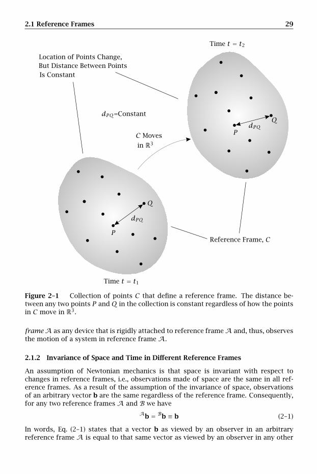
In order to visualize a reference frame, let C be an arbitrary collection of pointsthat move in R3 as shown in Fig. 2–1. Furthermore, suppose we choose two points Pand Q in C and let dPQ(t1) denote the distance between P and Q at some instant oftime t = t1. In general, at some later time t2 ≠ t1, every point in C will have moved to anew location in R3 and the distance between P and Q at t = t2 will be dPQ(t2). Then, ifdPQ(t1) = dPQ(t2) for all values of t1 and t2, the collection C will be a reference frame.
Using the aforementioned definition, many common objects can be used as refer-ence frames. For example, any three-dimensional rigid body (e.g., a cube, a sphere, or acylinder) can be chosen as a reference frame. In addition, any planar rigid object (e.g., asquare, a circle, or a triangle) can be chosen as a reference frame. However, given thedefinition, it is seen that an isolated point in R3 does not qualify as a reference frame.Furthermore, strictly speaking, a line in R3 also does not qualify as a reference framebecause the points on a line are, by definition, colinear.1 Finally, for most of the ap-plications considered in this book, a reference frame will typically be chosen based onphysically or geometrically meaningful objects.
In order to use reference frames systematically both in the theoretical developmentand the application of the theory to problems, we will use a calligraphic letter (e.g., A,B) to denote a reference frame.2 Consistent with this notation for a reference frame,we will use the terminology as viewed by an observer in reference frame A or, moresimply, in reference frame A to describe observations made about the motion of avector relative to reference frame A. Furthermore, we define an observer in reference
1While it is true that a line does not satisfy the definition of a reference frame, in certain applications,by abuse of the definition of a reference frame, we will sometimes take a line to be a reference frame. Insuch instances, the reference frame will be clear by context.
2It is noted that Kane and Levinson (1985) use a Roman italic letter to denote a reference frame. How-ever, in order to provide more clarity, we use a calligraphic letter to denote a reference frame.
2.1 Reference Frames 29
C Moves
in R3
Time t = t1
Time t = t2Location of Points Change,But Distance Between PointsIs Constant
Reference Frame, C
dPQ=Constant
dPQ
dPQ
P
P
Q
Q
Figure 2–1 Collection of points C that define a reference frame. The distance be-tween any two points P andQ in the collection is constant regardless of how the pointsin C move in R3.
frameA as any device that is rigidly attached to reference frameA and, thus, observesthe motion of a system in reference frame A.
2.1.2 Invariance of Space and Time in Different Reference Frames
An assumption of Newtonian mechanics is that space is invariant with respect tochanges in reference frames, i.e., observations made of space are the same in all ref-erence frames. As a result of the assumption of the invariance of space, observationsof an arbitrary vector b are the same regardless of the reference frame. Consequently,for any two reference frames A and B we have
Ab = Bb ≡ b (2–1)
In words, Eq. (2–1) states that a vector b as viewed by an observer in an arbitraryreference frame A is equal to that same vector as viewed by an observer in any other
30 Chapter 2. Kinematics
reference frame B.Next, for any system of interest, it is desirable to specify a quantity that param-
eterizes the motion, i.e., it is desirable to specify a quantity whose value determinesthe values of all other quantities of interest. Such a quantity is referred to as the inde-pendent variable. As its name implies, the independent variable does not depend onother quantities in the system. However, other quantities depend on the independentvariable. The most convenient type of independent variable is one that is independentof the reference frame. In Newtonian mechanics, the most commonly chosen indepen-dent variable is time. In this book we will generally use the variable t to denote timeand, with few exceptions, will choose time as the independent variable. Then, similarto the assumption that observations of space are the same in all reference frames, it isan assumption of Newtonian mechanics that time is invariant with respect to referenceframe, i.e., observations of time are the same in all reference frames. Consequently,for any two reference frames A and B we have
At = Bt ≡ t (2–2)
In words, Eq. (2–2) states that time as viewed by an observer in an arbitrary referenceframe A is equal to time as viewed by an observer in any other reference frame B.
2.1.3 Inertial and Noninertial Reference Frames
Reference frames are classified as either inertial or noninertial. An inertial or Newto-nian reference frame is one whose points are either absolutely fixed in space or at mosttranslate relative to an absolutely fixed set of points with the same constant velocity.A noninertial or non-Newtonian reference frame is one whose points accelerate withtime. It is an axiom of Newtonian mechanics that inertial reference frames exist andthat the laws of mechanics are valid only in an inertial reference frame.3 In general,we will use the calligraphic letter F to denote a fixed inertial reference frame, the cal-ligraphic letter N to denote a general (nonfixed but possibly uniform velocity) inertialreference frame, and any other calligraphic letter (e.g., A, B) to denote a noninertialreference frame.
2.2 Coordinate Systems
Once a set of reference frames has been chosen to make observations regarding themotion of a system, the next step is to quantify or realize the motion of the systemby choosing a set of coordinate systems that are fixed in each of the chosen referenceframes. It is important to understand that, while they may seem to be the same, areference frame and a coordinate system are distinct entities. We recall that a refer-ence frame is a collection of points such that the distance between any two points isconstant. However, it is seen that the definition of a reference frame does not directlyprovide any means of measuring the observations that may be made of the motionby an observer fixed in the reference frame. A coordinate system provides such ameasurement system. In particular, the following information is required in order tospecify a coordinate system that is fixed in a particular reference frame A: (a) a point
3The principle of Galilean invariance or Newtonian relativity states that the fundamental laws of me-chanics are the same in all inertial reference frames.
2.2 Coordinate Systems 31
fixed in A called the origin, the point from which all distances are measured in refer-ence frame A, and (b) a basis, which is a set of three linearly independent directionsthat are fixed in reference frame A; the basis provides a way to resolve vectors in R3.
Given the definition of a coordinate system, it is seen that, not only must a co-ordinate system be fixed in a unique reference frame, but it is also the case that acoordinate system cannot be fixed simultaneously in two distinct reference frames.Furthermore, while in principle any set of three linearly independent vectors can bechosen as a basis for a coordinate system, recall from Chapter 1 that it is most con-venient to use a so-called orthonormal basis (i.e., a set of mutually orthogonal unitvectors) in which to resolve vectors. Because of its convenience, from this point for-ward we will restrict our attention to orthonormal bases. Consequently, the basis mustsatisfy the following properties:
Property 1: The basis vectors e1, e2, and e3 are unit vectors, i.e.,
e1 · e1 = 1e2 · e2 = 1e3 · e3 = 1
(2–3)
Property 2: The basis vectors e1, e2, and e3 are mutually orthogonal, i.e.,
e1 · e2 = e2 · e1 = 0e1 · e3 = e3 · e1 = 0e2 · e3 = e3 · e2 = 0
(2–4)
Property 3: The basis vectors e1, e2, and e3 form a right-handed system, i.e.,
e1 × e2 = e3
e2 × e3 = e1
e3 × e1 = e2
(2–5)
We note that a basis that satisfies Properties 1 – 3 is called a right-handed orthonormalbasis. Figure 2–2 shows a schematic that provides a way to remember the right-handrule of Eq. (2–5). The arrows in Fig. 2–2 indicate the direction of positive orientation ofthe vector products given in Eq. (2–5); any vector product taken in the direction of thearrows yields a positive result while any vector product taken in the direction oppositethe arrows yields a negative result. It is noted that a right-handed system satisfies theproperty
e3 · (e1 × e2) = 1 (2–6)
It is important to understand that the set e1,e2,e3 must always be ordered suchthat Eq. (2–6) is satisfied (we note that the right-handed system as described in Eq. (2–5)is consistent with the orientation shown in Fig. 1–4 on page 8). Then, given a coordinatesystem fixed in a particular reference frame A, any vector b in R3 can be expressed inthe basis e1,e2,e3 corresponding to the chosen coordinate system as
b = b1e1 + b2e2 + b3e3 (2–7)
In other words, given a reference frame A and a basis e1,e2,e3 corresponding to acoordinate system fixed in A, for every vector b there exist scalar coefficients b1, b2,and b3 (which, in general, change with time), such that b can be represented in thebasis e1,e2,e3.

32 Chapter 2. Kinematics
e1
e2 e3
Figure 2–2 Schematic of right-hand rule corresponding to Eq. (2–5).
2.3 Rate of Change of Scalar and Vector Functions
2.3.1 Rate of Change of a Scalar Function
Suppose we are given a scalar function x(t) where x(t) ∈ R is a function of the pa-rameter t ∈ R. Then the rate of change of x(t) is defined as
dxdt
≡ lim∆t→0
x(t +∆t)− x(t)∆t
(2–8)
It is seen from the limit in Eq. (2–8) that, because x(t) does not depend on any par-ticular direction in R3, its rate of change dx/dt is independent of the reference frame.As a result, observers in all reference frames see exactly the same rate of change ofa scalar function, and the notation dx/dt has only one meaning (namely, that of thewell known calculus derivative).
2.3.2 Rate of Change of a Vector Function
It is seen from the previous discussion that observers in different reference frames allsee the same rate of change of a scalar function of time. Likewise, given an arbitraryvector function of time, at every instant of time observers in all reference frames seethe same vector. In other words, a vector is independent of the reference frame inwhich it is observed. However, unlike a scalar function of time, observers in differentreference frames do not see the same rate of change of a vector function of time. Con-trariwise, observers fixed in different reference frames will, in general, make differentobservations about the rate of change of a vector function of time. As a result, thephrase “rate of change of a vector” must always be qualified by stating explicitly thereference frame in which the observation is being made.
A precise notion of the rate of change of a vector function of time is given as fol-lows. Given an arbitrary reference frame A, the rate of change of a vector in referenceframe A is defined as
Adbdt
=A
lim∆t→0
b(t +∆t)− b(t)∆t
(2–9)
where the notationA
lim∆t→0
(2–10)
2.3 Rate of Change of Scalar and Vector Functions 33
means that the limit is taken by an observer fixed in reference frame A and Ad/dt isthe rate of change operator as viewed by an observer in reference frame A. In otherwords, the limit in Eq. (2–9) is being computed based on how the vector b appears tobe changing to an observer in reference frame A. Using the definition of Eq. (2–9), avector b is said to be fixed in a reference frame A if the following condition holds forall time:
Adbdt
= 0 (2–11)
In other words, if a vector b always appears to always have the same magnitude anddirection to an observer in reference frame A, its rate of change in reference frame Ais zero.
Suppose now that we choose to express an arbitrary vector b in terms of an or-thonormal basis (see Section 2.2 for the definition of an orthonormal basis) e1,e2,e3.Then b can be written as
b = b1e1 + b2e2 + b3e3 (2–12)
Furthermore, suppose that the basis e1,e2,e3 is fixed in reference frame A. Thenthe rate of change of b as viewed by an observer in reference frame A is defined bythe following limit:
Adbdt
= lim∆t→0
3∑i=1
bi(t +∆t)− bi(t)∆t
ei (2–13)
Observing that the limit and the summation are interchangeable, Eq. (2–13) can bewritten as
Adbdt
=3∑i=1
lim∆t→0
bi(t +∆t)− bi(t)∆t
ei (2–14)
Now, because b1, b2, and b3 are scalar functions of t, we have
dbidt
= lim∆t→0
bi(t +∆t)− bi(t)∆t
, (i = 1,2,3) (2–15)
where we note that bi , (i = 1,2,3) are scalar functions of t and hence their rates ofchange are independent of the choice of the reference frame. Consequently, Adb/dtcan be written as
Adbdt
= db1
dte1 + db2
dte2 + db3
dte3 = b1e1 + b2e2 + b3e3 (2–16)
Now, consistent with the definition given in Eq. (2–11) of a vector fixed in a referenceframe, it is observed in Eq. (2–16) that, because b is expressed in a basis e1,e2,e3 thatis fixed in reference frame A, the rate of change b in reference frame A is obtained bydifferentiating only the components of b (because, by Eq. (2–11), the rates of changeof the basis vectors in reference frame A are all zero). Consequently, when a vector isexpressed in a basis fixed in a reference frameA, it appears to an observer in referenceframe A that only the components of the vector are changing with time.
From the definition of the rate of change of an arbitrary vector in an arbitraryreference frame, it is seen that observers in different reference frames will see differentrates of change of the vector b. In other words, for two distinct reference frames Aand B, it will generally be the case that
Adbdt
≠Bdbdt
(2–17)
34 Chapter 2. Kinematics
Now, because the fundamental postulates of classical Newtonian mechanics, namelyNewton’s and Euler’s laws, are valid only when the motion is viewed by an observerin an inertial reference frame, we will ultimately be interested in obtaining the rate ofchange of a vector as viewed by an observer in an inertial reference frame. Thus, toavoid confusion in presenting the theory, the symbol N will always be used to denotean observation in an inertial reference frame.
2.3.3 Rate of Change of a Scalar Function of a Vector
A particular class of scalar functions whose rate of change is of interest in dynamics isthe class of scalar functions of vectors where the vectors are themselves functions oftime. Consider a scalar function F of a single vector b, i.e., F = F(b). Furthermore, letb be a function of time, i.e., b = b(t). As seen above, because F is a scalar function, itsrate of change is independent of the reference frame and is given as dF/dt. Supposenow b is resolved in a basis e1,e2,e3, where e1,e2,e3 is fixed in a reference frameA. Then b can be expressed as
b = b1e1 + b2e2 + b3e3 (2–18)
where b1, b2, and b3 are the components of b in the basis e1,e2,e3 that is fixed inA. Moreover, because the output of the function F is a scalar, we have
F(b) = F(b1, b2, b3) (2–19)
Equation (2–19) merely states that, because F is a scalar function, it depends only onthe components of b and not on the basis vectors. Then, computing the rate of changeof F in Eq. (2–19) and applying the chain rule, we obtain
dFdt
= ∂F∂b1
db1
dt+ ∂F∂b2
db2
dt+ ∂F∂b3
db3
dt(2–20)
Using the fact that the basis e1,e2,e3 forms a mutually orthogonal set, Eq. (2–20) canbe rewritten as
dFdt
=(∂F∂b1
e1 + ∂F∂b2
e2 + ∂F∂b3
e3
)·(db1
dte1 + db2
dte2 + db3
dte3
)(2–21)
Using the definition of rate of change of a vector in a reference frame A as given inEq. (2–16), Eq. (2–21) can be written more compactly as
dFdt
= ∇bF ·Adbdt
≡ ∂F∂b
·Adbdt
(2–22)
where
∇bF = ∂F∂b (2–23)
is the gradient of F with respect to b. Now, because both the gradient of F and thevector b can be expressed in a basis fixed in any reference frame, the result of Eq. (2–22) is valid in any reference frame.

2.4 Position, Velocity, and Acceleration 35
2.3.4 Rates of Change of Common Functions of Vectors
Let b and c be vectors in R3 and let k be a scalar. Then the following is a list of basicrules for computing the rates of change of common functions of vectors in an arbitraryreference frame A:
Addt(b+ c) =
Adbdt
+Adcdt
(2–24)
Addt(kb) = k
Adbdt
(2–25)
Addt(b× c) =
Adbdt
× c+ b×Adcdt
(2–26)
Addt(b · c) =
Adbdt
· c+ b ·Adcdt
≡ ddt(b · c) (2–27)
Addt(b⊗ c) =
Adbdt
⊗ c+ b⊗Adcdt
(2–28)
We remind the reader that, because the rate of change of a scalar function is indepen-dent of the reference frame, we have stated explicitly that the rate of change of thefunction b · c in Eq. (2–27) does not depend on the choice of the reference frame A.
2.4 Position, Velocity, and Acceleration
A particle (or point) is defined as an object that lies in three-dimensional Euclideanspace R3 and has no dimension, i.e., a particle occupies no space. Consider a particlemoving in R3 relative to a reference frame A as shown in Fig 2–3.
Point O Fixed in
A
Reference Frame A Particle
r
O
P
Figure 2–3 Particle moving relative to a reference frame A in three-dimensionalEuclidean space R3.
The position of the particle describes the location of the particle relative to a pointO fixed in A and is denoted r. The position of a particle is a function of a scalarparameter t (generally speaking, time), i.e., r = r(t). By varying t, the path or trajectoryof the particle is defined. In particular, when the motion of the particle is observed in
36 Chapter 2. Kinematics
reference frame A, we say that the particle subtends a trajectory relative to referenceframe A. Given r(t), the velocity of the particle as viewed by an observer in referenceframe A, denoted Av = Av(t), is the rate of change of the position relative to A andis defined as
Av =Adrdt
=A
lim∆t→0
r(t +∆t)− r(t)∆t
(2–29)
where we have used the definition of the limit as given in Eq. (2–10).4 Given Av(t), thespeed of the particle in reference frame A, denoted Av , is defined as
Av = ‖Av(t)‖ =√Av(t) · Av(t) (2–30)
Given Av(t), the acceleration of the particle in reference frameA, denoted Aa = Aa(t),is the rate of change of Av and is defined as
Aa =Addt
(Av
)=Addt
(Adrdt
)=
Alim∆t→0
Av(t +∆t)−Av(t)∆t
(2–31)
A point P in R3 is said to be fixed relative to reference frame A if its velocity andacceleration in reference frame A are both zero, i.e., P is fixed in A if Av ≡ 0 andAa ≡ 0. The distance traveled by a particle in a reference frame A during a timeinterval t ∈
[t0, tf
]is called the arc-length in reference frame A. The arc-length is
denoted by the scalar variable As, where As satisfies the differential equation
ddt
(As)= As ≡ Av (2–32)
and Av is obtained from Eq. (2–30); we note once again that, because As is a scalar, itsrate of change is independent of reference frame. Integrating Eq. (2–32) from t0 to t,we obtain
As(t)−As(t0) =∫ tt0
ddt
(As)dτ =
∫ tt0
Av(τ)dτ (2–33)
Note that, because Av is nonnegative, the quantity As(t)−As(t0)must also be nonneg-ative, i.e., As(t)−As(t0) ≥ 0. Finally, because As and Av are scalars, for compactnesswe will often omit the left superscript and simply use the notation v and s to denotespeed and arc-length, respectively. In the case where the left superscript is omitted,the discussion will always state explicitly the reference frame in which observationsare being made.
It is important to understand that, while the definitions above are computed rel-ative to a particular reference frame (in this case the reference frame A), the abovedefinitions do not assume a particular coordinate system, i.e., the above definitionsare coordinate-free but not reference frame-free.
4It is important to understand that the notation Av is merely a shorthand for Adr/dt. In other words,when we write Av, we mean that the vector Av arises from taking the rate of change of another vector(in this case position) in reference frame A. Furthermore, it is important to understand that, althoughAv arises from taking the rate of change of r in reference frame A, the quantity Av is itself a vector.Consequently, by assumption (see Section 2.1.2) observations of the vector Av are the same in all referenceframes.
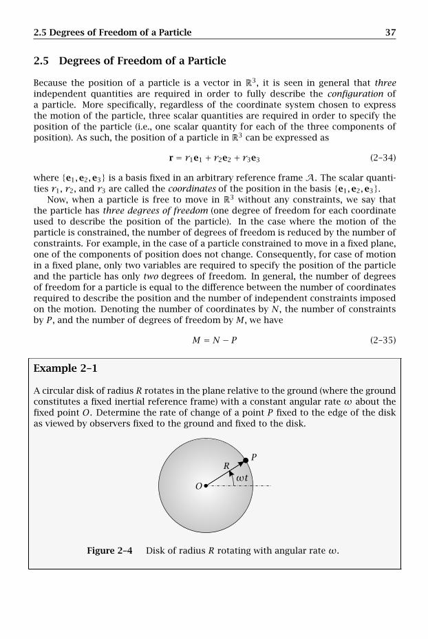
2.5 Degrees of Freedom of a Particle 37
2.5 Degrees of Freedom of a Particle
Because the position of a particle is a vector in R3, it is seen in general that threeindependent quantities are required in order to fully describe the configuration ofa particle. More specifically, regardless of the coordinate system chosen to expressthe motion of the particle, three scalar quantities are required in order to specify theposition of the particle (i.e., one scalar quantity for each of the three components ofposition). As such, the position of a particle in R3 can be expressed as
r = r1e1 + r2e2 + r3e3 (2–34)
where e1,e2,e3 is a basis fixed in an arbitrary reference frame A. The scalar quanti-ties r1, r2, and r3 are called the coordinates of the position in the basis e1,e2,e3.
Now, when a particle is free to move in R3 without any constraints, we say thatthe particle has three degrees of freedom (one degree of freedom for each coordinateused to describe the position of the particle). In the case where the motion of theparticle is constrained, the number of degrees of freedom is reduced by the number ofconstraints. For example, in the case of a particle constrained to move in a fixed plane,one of the components of position does not change. Consequently, for case of motionin a fixed plane, only two variables are required to specify the position of the particleand the particle has only two degrees of freedom. In general, the number of degreesof freedom for a particle is equal to the difference between the number of coordinatesrequired to describe the position and the number of independent constraints imposedon the motion. Denoting the number of coordinates by N, the number of constraintsby P , and the number of degrees of freedom by M , we have
M = N − P (2–35)
Example 2–1
A circular disk of radius R rotates in the plane relative to the ground (where the groundconstitutes a fixed inertial reference frame) with a constant angular rate ω about thefixed point O. Determine the rate of change of a point P fixed to the edge of the diskas viewed by observers fixed to the ground and fixed to the disk.
ωtO
PR
Figure 2–4 Disk of radius R rotating with angular rate ω.
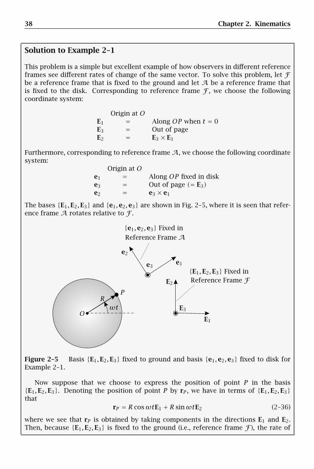
38 Chapter 2. Kinematics
Solution to Example 2–1
This problem is a simple but excellent example of how observers in different referenceframes see different rates of change of the same vector. To solve this problem, let Fbe a reference frame that is fixed to the ground and let A be a reference frame thatis fixed to the disk. Corresponding to reference frame F , we choose the followingcoordinate system:
Origin at OE1 = Along OP when t = 0E3 = Out of pageE2 = E3 × E1
Furthermore, corresponding to reference frameA, we choose the following coordinatesystem:
Origin at Oe1 = Along OP fixed in diske3 = Out of page (= E3)e2 = e3 × e1
The bases E1,E2,E3 and e1,e2,e3 are shown in Fig. 2–5, where it is seen that refer-ence frame A rotates relative to F .
e1,e2,e3 Fixed in
E1,E2,E3 Fixed in
Reference Frame A
Reference Frame F
ωt
e1
e2
e3
E1
E2
E3O
PR
Figure 2–5 Basis E1,E2,E3 fixed to ground and basis e1,e2,e3 fixed to disk forExample 2–1.
Now suppose that we choose to express the position of point P in the basisE1,E2,E3. Denoting the position of point P by rP , we have in terms of E1,E2,E3that
rP = R cosωtE1 + R sinωtE2 (2–36)
where we see that rP is obtained by taking components in the directions E1 and E2.Then, because E1,E2,E3 is fixed to the ground (i.e., reference frame F ), the rate of

2.6 Relative Position, Velocity, and Acceleration 39
change of rP as viewed by an observer in reference frameF is obtained using Eq. (2–16)as
Fddt(rP ) = −Rω sinωtE1 + Rω cosωtE2 (2–37)
where it is emphasized in Eq. (2–37) that the basis E1,E2,E3 is fixed in referenceframe F .
Next, suppose that we express the position of point P in terms of the basise1,e2,e3. We then have
rP = Re1 (2–38)
where we see from Eq. (2–38) that, at every instant of the motion, rP lies along thedirection e1. Then, because e1 is fixed in reference frame A, the rate of change of rPin reference frame A is obtained using Eq. (2–16) as
Addt(rP ) = dRdt e1 = 0 (2–39)
where we note that R is constant and, hence, dR/dt = 0.
2.6 Relative Position, Velocity, and Acceleration
Consider two points Q and P with positions rQ and rP , respectively. Furthermore, letA be a reference frame in which observations are made about the motion of points Qand P . Then the position of P relative to Q, denoted rP/Q, is defined as
rP/Q = rP − rQ (2–40)
Given rP/Q, the velocity of P relative to Q as viewed by an observer in reference frameA, denoted AvP/Q, is defined as the rate of change of ArP/Q as viewed by an observerin reference frame A, i.e.,
AvP/Q =Addt
(rP/Q
) = AvP −AvQ (2–41)
Finally, the acceleration of P relative to Q as viewed by an observer in reference frameA, denoted AaP/Q, is defined as the rate of change of AvP/Q in the reference frame A,i.e., is defined as
AaP/Q =Addt
(AvP/Q
)=Ad2
dt2(rP/Q
) = AaP −AaQ (2–42)
2.7 Rectilinear Motion
The simplest motion is that of a particle P moving in a straight line. Such motion iscalled rectilinear motion. Suppose that we choose to describe the rectilinear motion ofa particle as viewed by an observer in a fixed reference frame F . Because the motion is
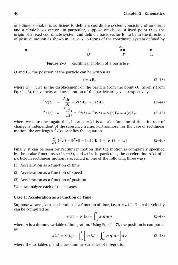
40 Chapter 2. Kinematics
one-dimensional, it is sufficient to define a coordinate system consisting of an originand a single basis vector. In particular, suppose we choose a fixed point O as theorigin of a fixed coordinate system and define a basis vector Ex to be in the directionof positive motion as shown in Fig. 2–6. In terms of the coordinate system defined by
Ex
x
O P
Figure 2–6 Rectilinear motion of a particle P .
O and Ex , the position of the particle can be written as
r = xEx (2–43)
where x = x(t) is the displacement of the particle from the point O. Given r fromEq. (2–43), the velocity and acceleration of the particle are given, respectively, as
Fv(t) =Fdrdt
= x(t)Ex = v(t)Ex (2–44)
Fa(t) =F d2rdt2
≡ F r(t) = F v(t) = x(t)Ex = a(t)Ex (2–45)
where we note once again that, because x(t) is a scalar function of time, its rate ofchange is independent of the reference frame. Furthermore, for the case of rectilinearmotion, the arc-length Fs(t) satisfies the equation
ddt
(Fs)= ‖Fv‖ = ‖v(t)Ex‖ = |v(t)| = |x| (2–46)
Finally, it can be seen for rectilinear motion that the motion is completely specifiedby the scalar functions x(t), v(t), and a(t). In particular, the acceleration a(t) of aparticle in rectilinear motion is specified in one of the following three ways:
(1) Acceleration as a function of time
(2) Acceleration as a function of speed
(3) Acceleration as a function of position
We now analyze each of these cases.
Case 1: Acceleration as a Function of Time
Suppose we are given acceleration as a function of time, i.e., a = a(t). Then the velocitycan be computed as
v(t) = v(t0)+∫ tt0a(η)dη (2–47)
where η is a dummy variable of integration. Using Eq. (2–47), the position is computedas
x(t) = x(t0)+∫ tt0
[v(t0)+
∫ νt0a(η)dη
]dν (2–48)
where the variables η and ν are dummy variables of integration.
2.7 Rectilinear Motion 41
Case 2: Acceleration as a Function of Velocity
Suppose we are given acceleration as a function of velocity, i.e., a = a(v). Then, fromthe chain rule (Kreyszig, 1988) we have
a = a(v) = dvdt
= dvdxdxdt
= vdvdx
(2–49)
Furthermore, from Eq. (2–49) we have
vdvdx
= a(v) (2–50)
Separating variables in Eq. (2–50) gives
dx = vdva(v)
(2–51)
Then, integrating both sides of Eq. (2–51) we obtain
x − x0 =∫ vv0
ηdηa(η)
(2–52)
where η is a dummy variable of integration. Finally, solving Eq. (2–52) for x, we obtain
x = x0 +∫ vv0
ηdηa(η)
(2–53)
Also, via separation of variables we have
dt = dva= dva(v)
(2–54)
Integrating Eq. (2–54) we obtain
t − t0 =∫ vv0
dηa(η)
(2–55)
Rewriting Eq. (2–55), the time can be solved for as
t = t0 +∫ vv0
dηa(η)
(2–56)
Case 3: Acceleration as a Function of Position
Suppose we are given acceleration as a function of position, i.e., we are given a = a(x).Then we can write
a(x) = dvdt
= dvdxdxdt
= vdvdx
(2–57)
Separating variables in Eq. (2–57) we have
vdv = a(x)dx (2–58)
Integrating both sides of Eq. (2–58) gives∫ vv0
ηdη =∫ xx0
a(η)dη (2–59)
42 Chapter 2. Kinematics
where η is a dummy variable of integration. Therefore,
v2
2− v
20
2=∫ xx0
a(η)dη (2–60)
which implies that
v2 = v20 + 2
∫ xx0
a(η)dη (2–61)
Solving for v gives
v(x) =[v2
0 + 2∫ xx0
a(η)dη]1/2
(2–62)
Moreover, because v = dx/dt we have
dt = dxv
(2–63)
Integrating both sides of Eq. (2–63) gives
t − t0 =∫ xx0
dηv(η)
(2–64)
which implies that
t = t0 +∫ xx0
dηv(η)
(2–65)
where the expression for v(x) from Eq. (2–62) is used in Eqs. (2–64) and (2–65).
2.8 Using Noninertial Reference Frames to Describe Motion
While using an inertial coordinate system is appealing because of its simplicity, it isoften the case that observations regarding the motion of a system are made in a non-inertial reference frame. The two types of noninertial reference frames that are com-monly encountered in dynamics are accelerating and rotating reference frames. Usingthe definitions of a reference frame and a coordinate system from Section 2.2, in thissection we derive an expression for the time derivative of a vector when observationsof the vector are made in a rotating reference frame.
2.9 Rate of Change of a Vector in a Rotating Reference Frame
Let A and B be two reference frames such that B rotates relative to A. Furthermore,let E1,E2,E3 and e1,e2,e3 be orthonormal bases fixed in reference frames A andB, respectively. In addition, let O be a fixed point in R3 common to both referenceframes A and B. Next, let b be a vector in R3. A schematic of the reference frames Aand B, the orthonormal bases E1,E2,E3 and e1,e2,e3, and the vector b is shown inFig 2–7. Then b can then be expressed in the basis e1,e2,e3 as
b = b1e1 + b2e2 + b3e3 (2–66)
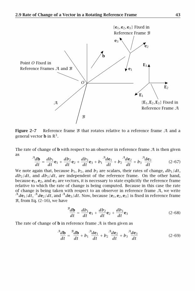
2.9 Rate of Change of a Vector in a Rotating Reference Frame 43
Point O Fixed in
A
e1,e2,e3 Fixed in
E1,E2,E3 Fixed in
Reference Frame A
Reference Frames A and B
Reference Frame B
e1
e2
e3
E1
E2
E3
b
O
B
Figure 2–7 Reference frame B that rotates relative to a reference frame A and ageneral vector b in R3.
The rate of change of b with respect to an observer in reference frame A is then givenas
Adbdt
= db1
dte1 + db2
dte2 + db3
dte3 + b1
Ade1
dt+ b2
Ade2
dt+ b3
Ade3
dt(2–67)
We note again that, because b1, b2, and b3 are scalars, their rates of change, db1/dt,db2/dt, and db3/dt, are independent of the reference frame. On the other hand,because e1, e2, and e3 are vectors, it is necessary to state explicitly the reference framerelative to which the rate of change is being computed. Because in this case the rateof change is being taken with respect to an observer in reference frame A, we writeAde1/dt, Ade2/dt, and Ade3/dt. Now, because e1,e2,e3 is fixed in reference frameB, from Eq. (2–16), we have
Bdbdt
= db1
dte1 + db2
dte2 + db3
dte3 (2–68)
The rate of change of b in reference frame A is then given as
Adbdt
=Bdbdt
+ b1
Ade1
dt+ b2
Ade2
dt+ b3
Ade3
dt(2–69)
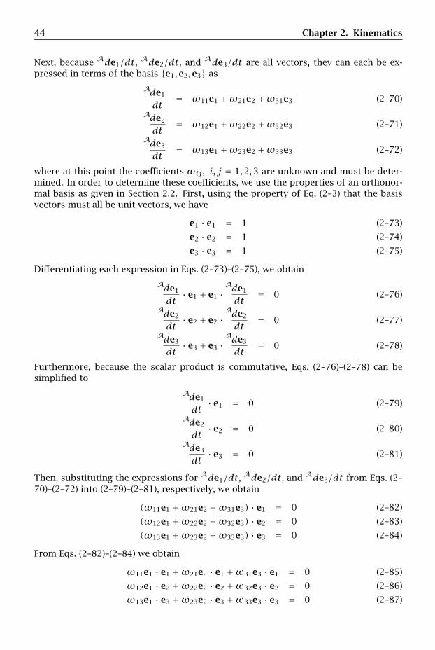
44 Chapter 2. Kinematics
Next, because Ade1/dt, Ade2/dt, and Ade3/dt are all vectors, they can each be ex-pressed in terms of the basis e1,e2,e3 as
Ade1
dt= ω11e1 +ω21e2 +ω31e3 (2–70)
Ade2
dt= ω12e1 +ω22e2 +ω32e3 (2–71)
Ade3
dt= ω13e1 +ω23e2 +ω33e3 (2–72)
where at this point the coefficients ωij, i, j = 1,2,3 are unknown and must be deter-mined. In order to determine these coefficients, we use the properties of an orthonor-mal basis as given in Section 2.2. First, using the property of Eq. (2–3) that the basisvectors must all be unit vectors, we have
e1 · e1 = 1 (2–73)
e2 · e2 = 1 (2–74)
e3 · e3 = 1 (2–75)
Differentiating each expression in Eqs. (2–73)–(2–75), we obtain
Ade1
dt· e1 + e1 ·
Ade1
dt= 0 (2–76)
Ade2
dt· e2 + e2 ·
Ade2
dt= 0 (2–77)
Ade3
dt· e3 + e3 ·
Ade3
dt= 0 (2–78)
Furthermore, because the scalar product is commutative, Eqs. (2–76)–(2–78) can besimplified to
Ade1
dt· e1 = 0 (2–79)
Ade2
dt· e2 = 0 (2–80)
Ade3
dt· e3 = 0 (2–81)
Then, substituting the expressions for Ade1/dt, Ade2/dt, and Ade3/dt from Eqs. (2–70)–(2–72) into (2–79)–(2–81), respectively, we obtain
(ω11e1 +ω21e2 +ω31e3) · e1 = 0 (2–82)
(ω12e1 +ω22e2 +ω32e3) · e2 = 0 (2–83)
(ω13e1 +ω23e2 +ω33e3) · e3 = 0 (2–84)
From Eqs. (2–82)–(2–84) we obtain
ω11e1 · e1 +ω21e2 · e1 +ω31e3 · e1 = 0 (2–85)
ω12e1 · e2 +ω22e2 · e2 +ω32e3 · e2 = 0 (2–86)
ω13e1 · e3 +ω23e2 · e3 +ω33e3 · e3 = 0 (2–87)
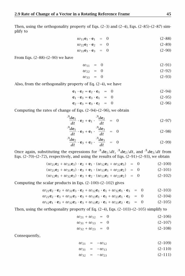
2.9 Rate of Change of a Vector in a Rotating Reference Frame 45
Then, using the orthogonality property of Eqs. (2–3) and (2–4), Eqs. (2–85)–(2–87) sim-plify to
ω11e1 · e1 = 0 (2–88)
ω22e2 · e2 = 0 (2–89)
ω33e3 · e3 = 0 (2–90)
From Eqs. (2–88)–(2–90) we have
ω11 = 0 (2–91)
ω22 = 0 (2–92)
ω33 = 0 (2–93)
Also, from the orthogonality property of Eq. (2–4), we have
e1 · e2 = e2 · e1 = 0 (2–94)
e1 · e3 = e3 · e1 = 0 (2–95)
e2 · e3 = e3 · e2 = 0 (2–96)
Computing the rates of change of Eqs. (2–94)–(2–96), we obtain
Ade1
dt· e2 + e1 ·
Ade2
dt= 0 (2–97)
Ade1
dt· e3 + e1 ·
Ade3
dt= 0 (2–98)
Ade2
dt· e3 + e2 ·
Ade3
dt= 0 (2–99)
Once again, substituting the expressions for Ade1/dt, Ade2/dt, and Ade3/dt fromEqs. (2–70)–(2–72), respectively, and using the results of Eqs. (2–91)–(2–93), we obtain
(ω21e2 +ω31e3) · e2 + e1 · (ω12e1 +ω32e3) = 0 (2–100)
(ω21e2 +ω31e3) · e3 + e1 · (ω13e1 +ω23e2) = 0 (2–101)
(ω12e1 +ω32e3) · e3 + e2 · (ω13e1 +ω23e2) = 0 (2–102)
Computing the scalar products in Eqs. (2–100)–(2–102) gives
ω21e2 · e2 +ω31e3 · e2 +ω12e1 · e1 +ω32e1 · e3 = 0 (2–103)
ω21e2 · e3 +ω31e3 · e3 +ω13e1 · e1 +ω23e1 · e2 = 0 (2–104)
ω12e1 · e3 +ω32e3 · e3 +ω13e2 · e1 +ω23e2 · e2 = 0 (2–105)
Then, using the orthogonality property of Eq. (2–4), Eqs. (2–103)–(2–105) simplify to
ω21 +ω12 = 0 (2–106)
ω31 +ω13 = 0 (2–107)
ω32 +ω23 = 0 (2–108)
Consequently,
ω21 = −ω12 (2–109)
ω31 = −ω13 (2–110)
ω32 = −ω23 (2–111)

46 Chapter 2. Kinematics
The expressions for Ade1/dt, Ade2/dt, and Ade3/dt can then be simplified to
Ade1
dt= ω21e2 +ω31e3 (2–112)
Ade2
dt= −ω21e1 +ω32e3 (2–113)
Ade3
dt= −ω31e1 −ω32e2 (2–114)
It can be seen from Eqs. (2–112)–(2–114) that only three of the original nine coefficientsremain, namely,ω21,ω31, andω32. For simplicity, the following substitutions are nowmade:
ω1 ≡ ω32
ω2 ≡ −ω31
ω3 ≡ ω21
(2–115)
Equations (2–112)–(2–114) can then be written as
Ade1
dt= ω3e2 −ω2e3 (2–116)
Ade2
dt= −ω3e1 +ω1e3 (2–117)
Ade3
dt= ω2e1 −ω1e2 (2–118)
Next, taking the scalar products of Ade2/dt, Ade3/dt, and Ade1/dt in Eq. (2–117),(2–118), and (2–116), respectively, with e3, e1, and e2, respectively, and applying theresults of Eqs. (2–97)–(2–99), we obtain ω1, ω2, and ω3 as
ω1 =Ade2
dt· e3 ≡ −e2 ·
Ade3
dt(2–119)
ω2 = −Ade1
dt· e3 ≡ e1 ·
Ade3
dt(2–120)
ω3 =Ade1
dt· e2 ≡ −e1 ·
Ade2
dt(2–121)
Suppose now that we define the vector
AωB =ω1e1 +ω2e2 +ω3e3 (2–122)
The quantity AωB is called the angular velocity of reference frame B as viewed by anobserver in reference frameA or, more simply, the angular velocity of B inA. In termsof the angular velocity, the vectors Ade1/dt, Ade2/dt, and Ade3/dt can be written as
Ade1
dt= ω3e2 −ω2e3 = AωB × e1 (2–123)
Ade2
dt= −ω3e1 +ω1e3 = AωB × e2 (2–124)
Ade3
dt= ω2e1 −ω1e2 = AωB × e3 (2–125)
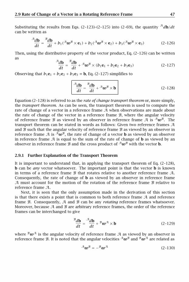
2.9 Rate of Change of a Vector in a Rotating Reference Frame 47
Substituting the results from Eqs. (2–123)–(2–125) into (2–69), the quantity Adb/dtcan be written as
Adbdt
=Bdbdt
+ b1(AωB × e1)+ b2(AωB × e2)+ b3(AωB × e3) (2–126)
Then, using the distributive property of the vector product, Eq. (2–126) can be writtenas
Adbdt
=Bdbdt
+AωB × (b1e1 + b2e2 + b3e3) (2–127)
Observing that b1e1 + b2e2 + b3e3 ≡ b, Eq. (2–127) simplifies to
Adbdt
=Bdbdt
+AωB × b (2–128)
Equation (2–128) is referred to as the rate of change transport theorem or, more simply,the transport theorem. As can be seen, the transport theorem is used to compute therate of change of a vector in a reference frame A when observations are made aboutthe rate of change of the vector in a reference frame B, where the angular velocityof reference frame B as viewed by an observer in reference frame A is AωB. Thetransport theorem can be stated in words as follows: Given two reference frames Aand B such that the angular velocity of reference frame B as viewed by an observer inreference frame A is AωB, the rate of change of a vector b as viewed by an observerin reference frame A is equal to the sum of the rate of change of b as viewed by anobserver in reference frame B and the cross product of AωB with the vector b.
2.9.1 Further Explanation of the Transport Theorem
It is important to understand that, in applying the transport theorem of Eq. (2–128),b can be any vector whatsoever. The important point is that the vector b is knownin terms of a reference frame B that rotates relative to another reference frame A.Consequently, the rate of change of b as viewed by an observer in reference frameA must account for the motion of the rotation of the reference frame B relative toreference frame A.
Next, it is seen that the only assumption made in the derivation of this sectionis that there exists a point that is common to both reference frame A and referenceframe B. Consequently, A and B can be any rotating reference frames whatsoever.Moreover, because A and B are arbitrary reference frames, the order of the referenceframes can be interchanged to give
Bdbdt
=Adbdt
+ BωA × b (2–129)
where BωA is the angular velocity of reference frame A as viewed by an observer inreference frame B. It is noted that the angular velocities AωB and BωA are related as
AωB = −BωA (2–130)

48 Chapter 2. Kinematics
2.9.2 Addition of Angular Velocities
Let A1, A2, and A3 be reference frames. Furthermore, let A1ωA2 be the angularvelocity of A2 as viewed by an observer in A1 and let A2ωA3 be the angular velocityof A3 as viewed by an observer in A2. Then from Eq. (2–128) we have
A1dbdt
=A2dbdt
+A1ωA2 × b (2–131)
A2dbdt
=A3dbdt
+A2ωA3 × b (2–132)
Now, substituting Eq. (2–132) into (2–131), we obtain
A1dbdt
=A3dbdt
+A2ωA3 × b+A1ωA2 × b (2–133)
Equation (2–133) can be rewritten as
A1dbdt
=A3dbdt
+(A1ωA2 +A2ωA3
)× b (2–134)
Now, from the transport theorem of Eq. (2–128), we also have that
A1dbdt
=A3dbdt
+A1ωA3 × b (2–135)
Setting Eqs. (2–135) and (2–134) equal, we obtain
A1ωA3 = A1ωA2 +A2ωA3 (2–136)
Equation (2–136) is called the angular velocity addition theorem and states that theangular velocity of a reference frame A3 in reference frame A1 is the sum of theangular velocity of A3 in A2 and the angular velocity of A2 in A1. Moreover, theangular velocity addition theorem can be extended to more than three reference framesas follows. Suppose we are given reference frames A1, . . . ,An such that AiωAi+1 (i =1, . . . , n − 1) are the angular velocities of reference frames Ai+1 (i = 1, . . . , n − 1)in reference frames Ai (i = 1, . . . , n − 1), respectively. Then the angular velocity ofreference frame An in reference frame A1, denoted A1ωAn , is given as
A1ωAn = A1ωA2 +A2ωA3 + · · · + An−1ωAn (2–137)
2.9.3 Angular Acceleration
The angular velocity defined in Eq. (2–122) defines the manner in which a referenceframe B rotates with time relative to another reference frameA. Now suppose that weapply the rate of change transport theorem of Eq. (2–128) to the angular velocity itself,i.e., we apply Eq. (2–128) to AωB. We then have that
Addt
(AωB
)=Bddt
(AωB
)+AωB × AωB (2–138)

2.9 Rate of Change of a Vector in a Rotating Reference Frame 49
Now, because AωB × AωB = 0, Eq. (2–138) reduces to
Addt
(AωB
)=Bddt
(AωB
)(2–139)
It is seen from Eq. (2–139) that the rate of change of AωB in reference frame A is thesame as the rate of change of AωB in reference frame B. The quantity
Addt
(AωB
)(2–140)
is called the angular acceleration of reference frame B in reference frame A. As aconvention, we use the variable α to denote angular acceleration, i.e., the quantity
AαB ≡Addt
(AωB
)=Bddt
(AωB
)(2–141)
is the angular acceleration of reference frame B in reference frame A. Now, fromEq. (2–130) we see that
AαB =Addt
(AωB
)= −
Addt
(BωA
)= −BαA (2–142)
which is similar to the result obtained for angular velocity as shown in Eq. (2–130).Suppose now that we compute the rate of change of A1ωA3 in reference frame A1
using the expression for A1ωA3 in Eq. (2–136). We then obtain
A1ddt
(A1ωA3
)=A1ddt
(A1ωA2 +A2ωA3
)(2–143)
Expanding Eq. (2–143) gives
A1ddt
(A1ωA3
)=A1ddt
(A1ωA2
)+A1ddt
(A2ωA3
)(2–144)
Applying the rate of change transport theorem of Eq. (2–128) to the second term inEq. (2–144), we have
A1ddt
(A1ωA3
)=A1ddt
(A1ωA2
)+A2ddt
(A2ωA3
)+A1ωA2 ×A2ωA3 (2–145)
Then, using the definition of angular acceleration as given in Eq. (2–141), the first andsecond terms of Eq. (2–145) can be written as
A1ddt
(A1ωA2
)= A1αA2
A2ddt
(A2ωA3
)= A2αA3
(2–146)
Equation (2–145) can then be written as
A1ddt
(A1ωA3
)= A1αA2 +A2αA3 +A1ωA2 ×A2ωA3 (2–147)
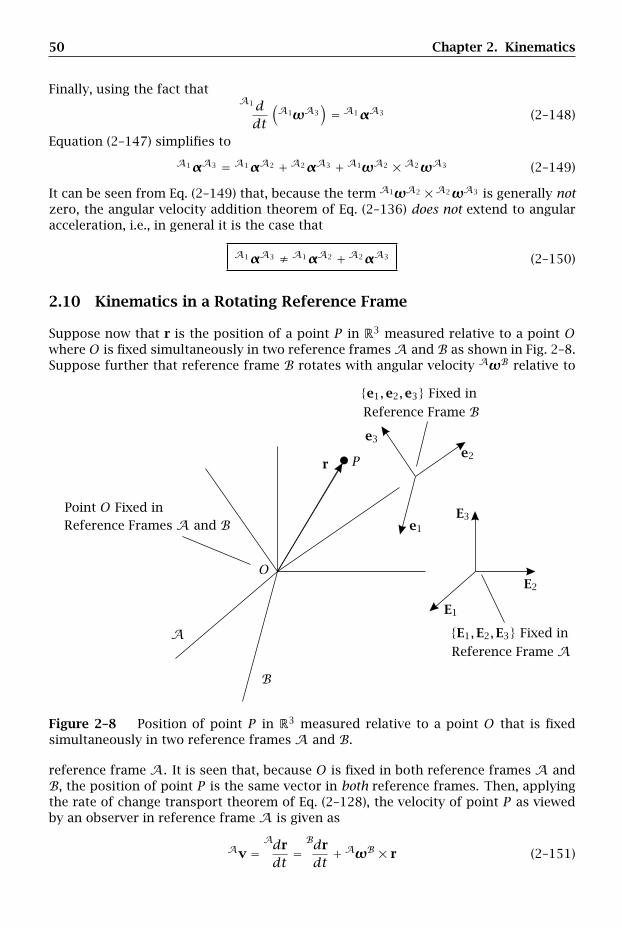
50 Chapter 2. Kinematics
Finally, using the fact thatA1ddt
(A1ωA3
)= A1αA3 (2–148)
Equation (2–147) simplifies to
A1αA3 = A1αA2 +A2αA3 +A1ωA2 ×A2ωA3 (2–149)
It can be seen from Eq. (2–149) that, because the term A1ωA2 ×A2ωA3 is generally notzero, the angular velocity addition theorem of Eq. (2–136) does not extend to angularacceleration, i.e., in general it is the case that
A1αA3 ≠ A1αA2 +A2αA3 (2–150)
2.10 Kinematics in a Rotating Reference Frame
Suppose now that r is the position of a point P in R3 measured relative to a point Owhere O is fixed simultaneously in two reference framesA and B as shown in Fig. 2–8.Suppose further that reference frame B rotates with angular velocity AωB relative to
Point O Fixed in
A
e1,e2,e3 Fixed in
E1,E2,E3 Fixed in
Reference Frame A
Reference Frames A and B
Reference Frame B
e1
e2
e3
E1
E2
E3
r
O
P
B
Figure 2–8 Position of point P in R3 measured relative to a point O that is fixedsimultaneously in two reference frames A and B.
reference frame A. It is seen that, because O is fixed in both reference frames A andB, the position of point P is the same vector in both reference frames. Then, applyingthe rate of change transport theorem of Eq. (2–128), the velocity of point P as viewedby an observer in reference frame A is given as
Av =Adrdt
=Bdrdt+AωB × r (2–151)
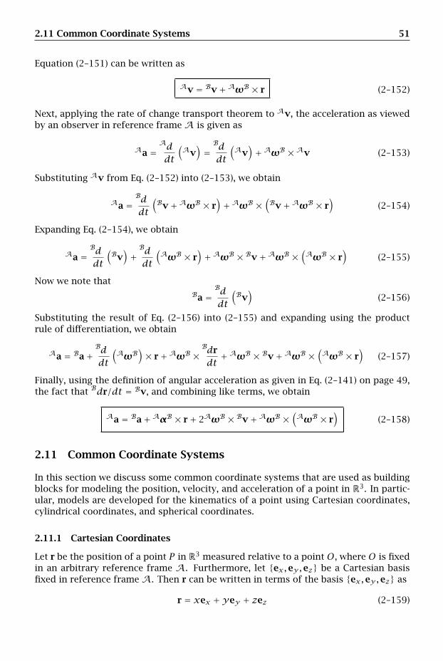
2.11 Common Coordinate Systems 51
Equation (2–151) can be written as
Av = Bv+AωB × r (2–152)
Next, applying the rate of change transport theorem to Av, the acceleration as viewedby an observer in reference frame A is given as
Aa =Addt
(Av
)=Bddt
(Av
)+AωB × Av (2–153)
Substituting Av from Eq. (2–152) into (2–153), we obtain
Aa =Bddt
(Bv+AωB × r
)+AωB ×
(Bv+AωB × r
)(2–154)
Expanding Eq. (2–154), we obtain
Aa =Bddt
(Bv)+Bddt
(AωB × r
)+AωB × Bv+AωB ×
(AωB × r
)(2–155)
Now we note thatBa =
Bddt
(Bv)
(2–156)
Substituting the result of Eq. (2–156) into (2–155) and expanding using the productrule of differentiation, we obtain
Aa = Ba+Bddt
(AωB
)× r+AωB ×
Bdrdt+AωB × Bv+AωB ×
(AωB × r
)(2–157)
Finally, using the definition of angular acceleration as given in Eq. (2–141) on page 49,the fact that Bdr/dt = Bv, and combining like terms, we obtain
Aa = Ba+AαB × r+ 2AωB × Bv+AωB ×(AωB × r
)(2–158)
2.11 Common Coordinate Systems
In this section we discuss some common coordinate systems that are used as buildingblocks for modeling the position, velocity, and acceleration of a point in R3. In partic-ular, models are developed for the kinematics of a point using Cartesian coordinates,cylindrical coordinates, and spherical coordinates.
2.11.1 Cartesian Coordinates
Let r be the position of a point P in R3 measured relative to a point O, where O is fixedin an arbitrary reference frame A. Furthermore, let ex,ey,ez be a Cartesian basisfixed in reference frame A. Then r can be written in terms of the basis ex,ey,ez as
r = xex +yey + zez (2–159)
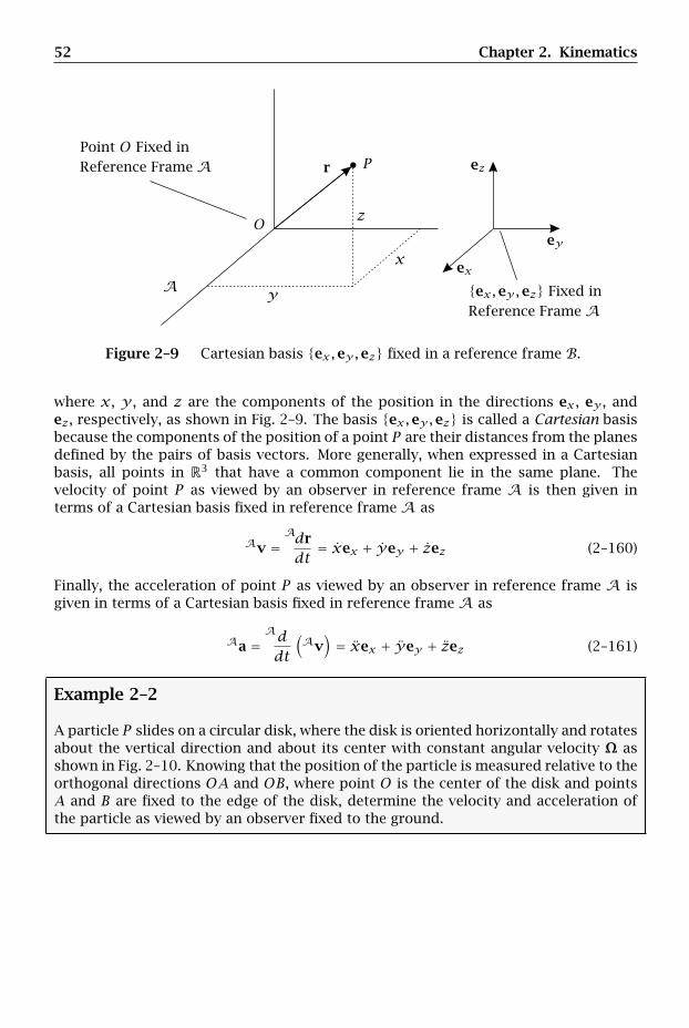
52 Chapter 2. Kinematics
Point O Fixed in
A ex,ey,ez Fixed in
Reference Frame A
Reference Frame A
ex
ey
ezr
x
y
zO
P
Figure 2–9 Cartesian basis ex,ey,ez fixed in a reference frame B.
where x, y , and z are the components of the position in the directions ex , ey , andez, respectively, as shown in Fig. 2–9. The basis ex,ey,ez is called a Cartesian basisbecause the components of the position of a point P are their distances from the planesdefined by the pairs of basis vectors. More generally, when expressed in a Cartesianbasis, all points in R3 that have a common component lie in the same plane. Thevelocity of point P as viewed by an observer in reference frame A is then given interms of a Cartesian basis fixed in reference frame A as
Av =Adrdt
= xex + yey + zez (2–160)
Finally, the acceleration of point P as viewed by an observer in reference frame A isgiven in terms of a Cartesian basis fixed in reference frame A as
Aa =Addt
(Av
)= xex + yey + zez (2–161)
Example 2–2
A particle P slides on a circular disk, where the disk is oriented horizontally and rotatesabout the vertical direction and about its center with constant angular velocity Ω asshown in Fig. 2–10. Knowing that the position of the particle is measured relative to theorthogonal directions OA and OB, where point O is the center of the disk and pointsA and B are fixed to the edge of the disk, determine the velocity and acceleration ofthe particle as viewed by an observer fixed to the ground.
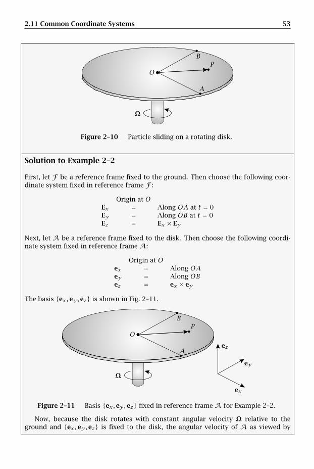
2.11 Common Coordinate Systems 53
A
B
OP
Ω
Figure 2–10 Particle sliding on a rotating disk.
Solution to Example 2–2
First, let F be a reference frame fixed to the ground. Then choose the following coor-dinate system fixed in reference frame F :
Origin at OEx = Along OA at t = 0Ey = Along OB at t = 0Ez = Ex × Ey
Next, let A be a reference frame fixed to the disk. Then choose the following coordi-nate system fixed in reference frame A:
Origin at Oex = Along OAey = Along OBez = ex × ey
The basis ex,ey,ez is shown in Fig. 2–11.
ex
ey
ezA
B
OP
Ω
Figure 2–11 Basis ex,ey,ez fixed in reference frame A for Example 2–2.
Now, because the disk rotates with constant angular velocity Ω relative to theground and ex,ey,ez is fixed to the disk, the angular velocity of A as viewed by
54 Chapter 2. Kinematics
an observer in reference frame F is given as
FωA = Ω = Ωez (2–162)
Furthermore, because ex,ey,ez is a Cartesian basis and the motion is confined tothe plane of the disk, the position of the particle P can be expressed in the basisex,ey,ez as
r = xex +yey (2–163)
The velocity of P as viewed by an observer fixed to the ground is then obtained fromEq. (2–128) as
Fv ≡Fdrdt
=Adrdt+ FωA × r (2–164)
Substituting r from Eq. (2–163) and FωA from Eq. (2–162) into (2–164) we have
Adrdt
= xex + yey (2–165)
FωA × r = Ωez × (xex +yey) = Ωxey −Ωyex (2–166)
Adding Eqs. (2–165) and (2–166), we obtain the velocity of the particle as viewed by anobserver fixed to the ground as
Fv = (x −Ωy)ex + (y +Ωx)ey (2–167)
Next, applying Eq. (2–128) to Fv, the acceleration of P as viewed by an observer fixedto the ground is given as
Fa ≡Fddt
(Fv)=Addt
(Fv)+ FωA × Fv (2–168)
Now, because Ω is constant in both magnitude and direction, we have
Addt
(Fv)
= (x −Ωy)ex + (y +Ωx)ey (2–169)
FωA × Fv = ΩEz ×[(x −Ωy)ex + (y +Ωx)ey
]= Ω(x −Ωy)ey −Ω(y +Ωx)ex= −(Ωy +Ω2x)ex + (Ωx −Ω2y)ey (2–170)
Adding the two expressions in Eqs. (2–169) and (2–170), we obtain the acceleration ofthe particle as viewed by an observer fixed to the ground as
Fa = (x − 2Ωy −Ω2x)ex + (y + 2Ωx −Ω2y)ey (2–171)
2.11 Common Coordinate Systems 55
2.11.2 Cylindrical Coordinates
Let r be the position of a point P in R3 measured relative to a point O, where O is fixedin an arbitrary reference frame A. Furthermore, let ex,ey,ez be a Cartesian basisforA. Recalling from Eq. (2–159) the expression for r in terms of the basis ex,ey,ez,we have
r = xex +yey + zez (2–172)
Suppose now that we make the following substitutions:
x = r cosθy = r sinθ (2–173)
wherer =
√x2 +y2
θ = tan−1(y/x
) (2–174)
Then r can be written as
r = r cosθex + r sinθey + zez= r(cosθex + sinθey)+ zez
(2–175)
Now leter = cosθex + sinθey (2–176)
Substituting the result of Eq. (2–176) into (2–175), the position is obtained as
r = rer + zez (2–177)
Using the fact ex and ey are orthogonal and that cos2θ + sin2θ = 1, it is seen thater is a unit vector. Furthermore, because er lies in the ex,ey-plane, it follows thater is orthogonal to ez. Consequently, er and ez can be used to define an alternateorthonormal basis. Denoting er and ez as the first and third basis vectors of this newbasis, the second basis vector can be obtained from the right-hand rule as
eθ = ez × er (2–178)
Substituting the expression for er from Eq. (2–176), we have
eθ = ez × (cosθex + sinθey) = − sinθex + cosθey (2–179)
Note that because eθ was obtained via the vector product of ez with er , it followsthat eθ is orthogonal to both ez and er . Furthermore, because both ez and er areorthogonal unit vectors, eθ is also a unit vector. The orthonormal basis er ,eθ,ez iscalled a cylindrical or radial-transverse basis and is shown in Fig. 2–12.
Suppose now that we define a reference frame B such that the basis er ,eθ,ez isfixed in B. Then, because er ,eθ,ez rotates with angular rate θ about the ez-direction,the angular velocity of B as viewed by an observer in A is given as
AωB = θez (2–180)
Applying the rate of change transport theorem of Eq. (2–128) to r using the expressionsfor r and AωB from Eqs. (2–177) and (2–180), respectively, the velocity of the particleas viewed by an observer in reference frame A is given as
Av =Adrdt
=Bdrdt+AωB × r (2–181)
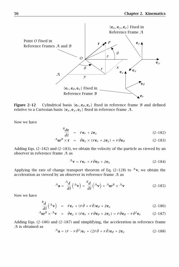
56 Chapter 2. Kinematics
Point O Fixed in
A
ex,ey,ez Fixed in
er ,eθ,ez Fixed in
Reference Frame A
Reference Frames A and B
Reference Frame Ber
eθ
ex
ey
ez
ezr
r x
y
zO
P
θ
θ
Figure 2–12 Cylindrical basis er ,eθ,ez fixed in reference frame B and definedrelative to a Cartesian basis ex,ey,ez fixed in reference frame A.
Now we have
Bdrdt
= rer + zez (2–182)
AωB × r = θez × (rer + zez) = r θeθ (2–183)
Adding Eqs. (2–182) and (2–183), we obtain the velocity of the particle as viewed by anobserver in reference frame A as
Av = rer + r θeθ + zez (2–184)
Applying the rate of change transport theorem of Eq. (2–128) to Av, we obtain theacceleration as viewed by an observer in reference frame A as
Aa =Addt
(Av
)=Bddt
(Av
)+AωB × Av (2–185)
Now we have
Bddt
(Av
)= rer + (r θ + r θ)eθ + zez (2–186)
AωB × Av = θez × (rer + r θeθ + zez) = r θeθ − r θ2er (2–187)
Adding Eqs. (2–186) and (2–187) and simplifying, the acceleration in reference frameA is obtained as
Aa = (r − r θ2)er + (2r θ + r θ)eθ + zez (2–188)

2.11 Common Coordinate Systems 57
Example 2–3
A collar slides freely along a rigid arm as shown in Fig. 2–13. The arm is hinged at oneof its ends to a point O, where O is fixed to the ground, and rotates about a directionthat is orthogonal to the plane of motion. Knowing that the position of the collar isdescribed by the variables r and θ, where r is the displacement of the collar relativeto point O and θ is the angle of the rod measured relative to a direction that is fixedto the ground, determine the velocity and acceleration of the collar as viewed by anobserver fixed to the ground.
r
O
P
θ
Figure 2–13 Collar sliding on a rotating arm.
Solution to Example 2–3
For this problem, it is convenient to define two reference frames. The first referenceframe, denoted F , is fixed to the ground while the second, denoted A, is fixed to thearm. Corresponding to reference frame F , we choose the following Cartesian coordi-nate system:
Origin at point OEx = To the rightEz = Out of pageEy = Ez × Ex
Corresponding to reference frame A, we choose the following cylindrical coordinatesystem:
Origin at point Oer = Along OPez = Out of pageeθ = ez × er
The bases Ex,Ey,Ez and er ,eθ,ez are shown in Fig. 2–14.
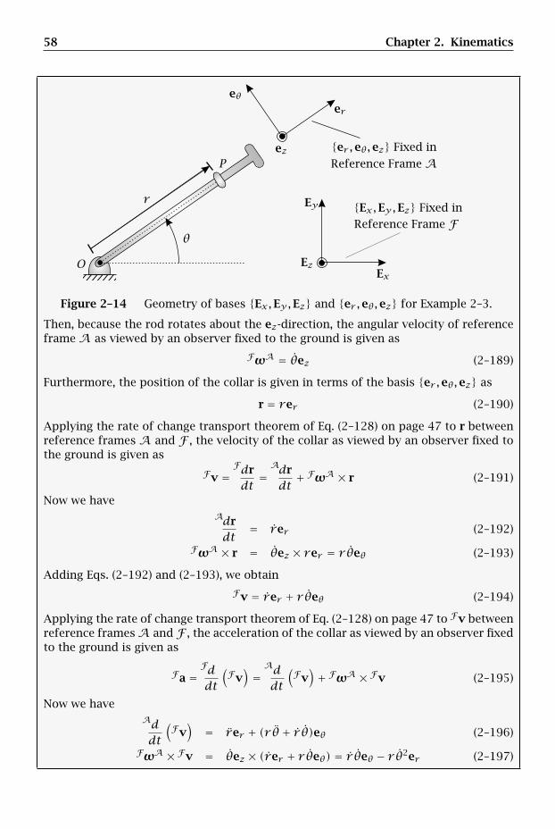
58 Chapter 2. Kinematics
Ex,Ey,Ez Fixed in
er ,eθ,ez Fixed in
Reference Frame A
Reference Frame F
er
eθ
ez
Ex
Ey
Ez
r
O
P
θ
Figure 2–14 Geometry of bases Ex,Ey,Ez and er ,eθ,ez for Example 2–3.
Then, because the rod rotates about the ez-direction, the angular velocity of referenceframe A as viewed by an observer fixed to the ground is given as
FωA = θez (2–189)
Furthermore, the position of the collar is given in terms of the basis er ,eθ,ez as
r = rer (2–190)
Applying the rate of change transport theorem of Eq. (2–128) on page 47 to r betweenreference frames A and F , the velocity of the collar as viewed by an observer fixed tothe ground is given as
Fv =Fdrdt
=Adrdt+ FωA × r (2–191)
Now we haveAdrdt
= rer (2–192)
FωA × r = θez × rer = r θeθ (2–193)
Adding Eqs. (2–192) and (2–193), we obtain
Fv = rer + r θeθ (2–194)
Applying the rate of change transport theorem of Eq. (2–128) on page 47 to Fv betweenreference framesA and F , the acceleration of the collar as viewed by an observer fixedto the ground is given as
Fa =Fddt
(Fv)=Addt
(Fv)+ FωA × Fv (2–195)
Now we haveAddt
(Fv)
= rer + (r θ + r θ)eθ (2–196)
FωA × Fv = θez × (rer + r θeθ) = r θeθ − r θ2er (2–197)
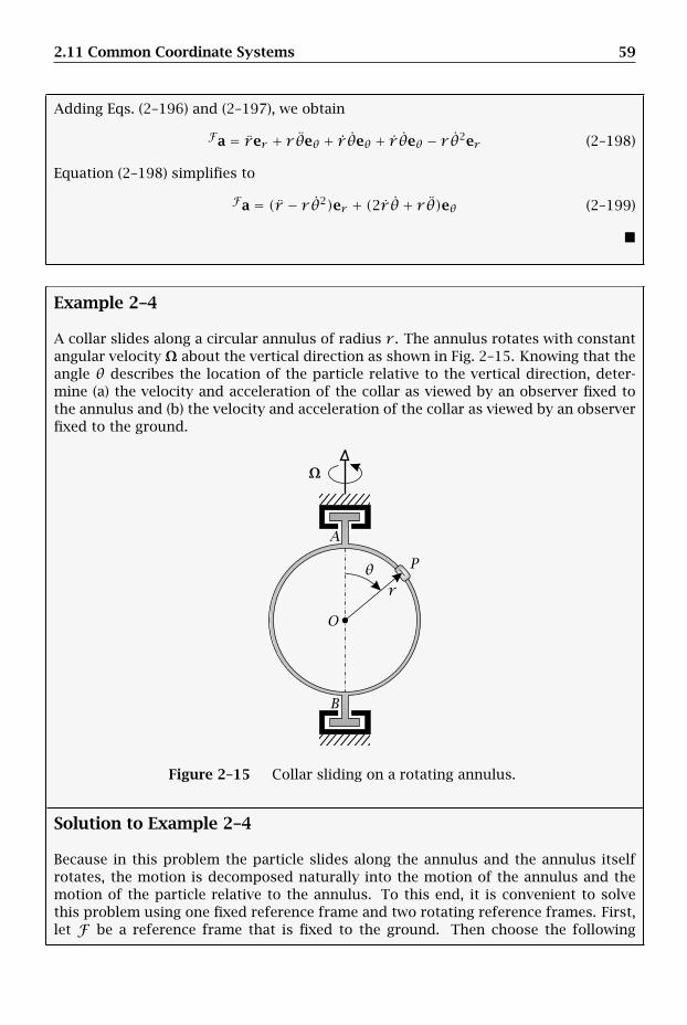
2.11 Common Coordinate Systems 59
Adding Eqs. (2–196) and (2–197), we obtain
Fa = rer + r θeθ + r θeθ + r θeθ − r θ2er (2–198)
Equation (2–198) simplifies to
Fa = (r − r θ2)er + (2r θ + r θ)eθ (2–199)
Example 2–4
A collar slides along a circular annulus of radius r . The annulus rotates with constantangular velocity Ω about the vertical direction as shown in Fig. 2–15. Knowing that theangle θ describes the location of the particle relative to the vertical direction, deter-mine (a) the velocity and acceleration of the collar as viewed by an observer fixed tothe annulus and (b) the velocity and acceleration of the collar as viewed by an observerfixed to the ground.
r
A
B
O
Pθ
Ω
Figure 2–15 Collar sliding on a rotating annulus.
Solution to Example 2–4
Because in this problem the particle slides along the annulus and the annulus itselfrotates, the motion is decomposed naturally into the motion of the annulus and themotion of the particle relative to the annulus. To this end, it is convenient to solvethis problem using one fixed reference frame and two rotating reference frames. First,let F be a reference frame that is fixed to the ground. Then choose the following
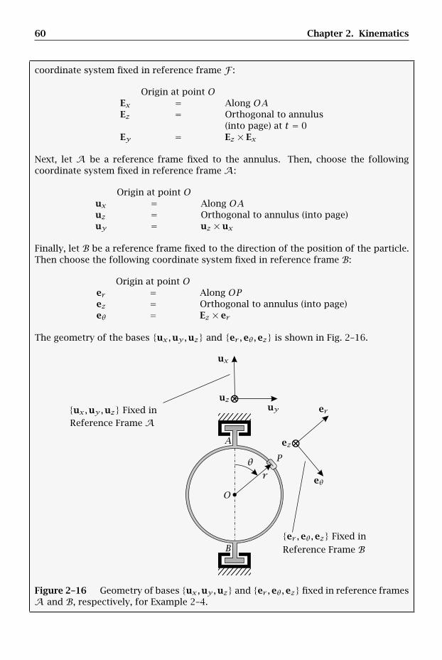
60 Chapter 2. Kinematics
coordinate system fixed in reference frame F :
Origin at point OEx = Along OAEz = Orthogonal to annulus
(into page) at t = 0Ey = Ez × Ex
Next, let A be a reference frame fixed to the annulus. Then, choose the followingcoordinate system fixed in reference frame A:
Origin at point Oux = Along OAuz = Orthogonal to annulus (into page)uy = uz × ux
Finally, let B be a reference frame fixed to the direction of the position of the particle.Then choose the following coordinate system fixed in reference frame B:
Origin at point Oer = Along OPez = Orthogonal to annulus (into page)eθ = Ez × er
The geometry of the bases ux,uy,uz and er ,eθ,ez is shown in Fig. 2–16.
ux,uy,uz Fixed in
er ,eθ,ez Fixed in
Reference Frame A
Reference Frame B
⊗
⊗er
eθ
ez
ux
uyuz
r
A
B
O
Pθ
Figure 2–16 Geometry of bases ux,uy,uz and er ,eθ,ez fixed in reference framesA and B, respectively, for Example 2–4.
2.11 Common Coordinate Systems 61
Using Fig. 2–16, we have
ux = cosθer − sinθeθ (2–200)
uy = sinθer + cosθeθ (2–201)
It is seen that the bases er ,eθ,ez and ux,uy,uz share a common direction uz = ez.Also, it is seen from Eqs. (2–200) and (2–201) that the bases er ,eθ,ez and ux,uy,uzare aligned when θ = 0.
(a) Velocity and Acceleration of Collar as Viewed by an Observer Fixed to Annulus
The position of the particle is given in terms of the basis er ,eθ,ez as
r = rer (2–202)
Now, because er ,eθ,ez is fixed in B and rotates with angular rate θ about the ez-direction relative to the annulus, the angular velocity of reference frame B in referenceframe A is given as
AωB = θez (2–203)
Then, applying the transport theorem of Eq. (2–128) on page 47, the velocity of thecollar in reference frame A is given as
Av =Bdrdt+AωB × r (2–204)
Noting that r is constant, we haveBdrdt
= 0 (2–205)
Also,AωB × r = θez × rer = r θeθ (2–206)
Adding the results of Eqs. (2–205) and (2–206), we obtain the velocity of the collar asviewed by an observer fixed to the annulus, Av, as
Av = r θeθ (2–207)
Applying Eq. (2–128) on page 47 to Av, the acceleration of the collar as viewed by anobserver to the annulus is given as
Aa =Bddt
(Av
)+AωB × Av (2–208)
Using Av from Eq. (2–207), we have
Bddt
(Av
)= r θeθ (2–209)
andAωB × Av = θez × r θeθ = −r θ2er (2–210)
Adding the results of Eqs. (2–209) and (2–210), we obtain the acceleration of the collaras viewed by an observer fixed to the annulus as
Aa = −r θ2er + r θeθ (2–211)
62 Chapter 2. Kinematics
(b) Velocity and Acceleration of Collar as Viewed by an Observer Fixed to Ground
The velocity and acceleration of the collar as viewed by an observer fixed to the groundcan be obtained using two different methods. The first method is to use a two-stageprocedure in which the rate of change transport theorem is applied between referenceframes B and A and again between reference frames A and F . The second methodis to apply the rate of change transport theorem directly between reference frames Band F . Each of these methods is now applied to this example.
Method 1: Two-Stage Application of Transport Theorem
In this method, the velocity of the collar as viewed by an observer fixed to the groundis obtained by applying Eq. (2–128) on page 47 between reference frames A and F as
Fv =Adrdt+ FωA × r = Av+ FωA × r (2–212)
Now, we already have Av from Eq. (2–207). Then, because the collar rotates relative tothe ground with angular velocity Ω about the ux-direction, we have
FωA = Ω = Ωux (2–213)
Using the expression for ux from Eq. (2–200), we have
FωA = Ω = Ω(cosθer − sinθeθ) = Ω cosθer −Ω sinθeθ (2–214)
Consequently, we obtain
FωA × r = (Ω cosθer −Ω sinθeθ)× rer = rΩ sinθez (2–215)
Adding Eq. (2–207) and (2–215), we obtain the velocity of the collar as viewed by anobserver fixed to the annulus as
Fv = r θeθ + rΩ sinθez (2–216)
Then, applying the transport theorem of Eq. (2–128) on page 47, the acceleration ofthe collar as viewed by an observer fixed to the annulus is given as
Fa =Addt
(Fv)+ FωA × Fv (2–217)
Now the quantityAd(Fv)/dt can itself be obtained using the rate of change transport
theorem between reference frames B and A as
Addt
(Fv)=Bddt
(Fv)+AωB × Fv (2–218)
Noting that r and Ω are constant and using Fv from Eq. (2–216), we have
Bddt
(Fv)= r θeθ + rΩθ cosθez (2–219)
2.11 Common Coordinate Systems 63
Furthermore,AωB × Fv = θez × (r θeθ + rΩ sinθez) = −r θ2er (2–220)
Adding the results of Eqs. (2–219) and (2–220), we have
Addt
(Fv)= r θeθ + rΩθ cosθez − r θ2er (2–221)
Next, FωA × Fv is obtained as
FωA × Fv = Ωux × (r θeθ + rΩ sinθez) (2–222)
Expanding Eq. (2–222), we obtain
FωA × Fv = rΩθux × eθ + rΩ2 sinθux × ez (2–223)
Then, using Eq. (2–200), we have
ux × eθ = (cosθer − sinθeθ)× eθ = cosθez (2–224)
ux × ez = (cosθer − sinθeθ)× ez = − sinθer − cosθeθ (2–225)
Substituting the results of Eqs. (2–224) and (2–225) into (2–223) gives
FωA × Fv = rΩθ cosθez + rΩ2 sinθ(− sinθer − cosθeθ) (2–226)
Simplifying Eq. (2–226), we obtain
FωA × Fv = −rΩ2 sin2θer − rΩ2 cosθ sinθeθ + rΩθ cosθez (2–227)
Adding Eqs. (2–221) and (2–227), we obtain the acceleration of the collar as viewed byan observer fixed to the annulus as
Fa = r θeθ + rΩθ cosθez − r θ2er
− rΩ2 sin2θer − rΩ2 cosθ sinθeθ + rΩθ cosθez(2–228)
Combining terms with common components in Eq. (2–228), we obtain the accelerationof the collar as viewed by an observer fixed to the ground as
Fa = −(r θ2 + rΩ2 sin2θ)er + (r θ − rΩ2 cosθ sinθ)eθ + 2rΩθ cosθez (2–229)
Method 2: One-Stage Application of Transport Theorem
The velocity of the collar as viewed by an observer fixed to the ground is obtainedby applying the rate of change transport theorem of Eq. (2–128) on page 47 betweenreference frames B and F as
Fv =Bdrdt+ FωB × r (2–230)
Now the angular velocity of reference frame B in reference frame F is obtained fromthe theorem of angular velocity addition as
FωB = FωA +AωB (2–231)
64 Chapter 2. Kinematics
Using the expressions for AωB and FωA from Eqs. (2–203) and (2–214), respectively,the angular velocity of reference frame B in reference frame F is obtained as
FωB = Ω cosθer − sinθeθ + θez (2–232)
Next we have
Bdrdt
= 0 (2–233)
FωB × r = (Ω cosθer −Ω sinθeθ + θez)× (rer )= r θeθ + rΩ sinθez (2–234)
Adding Eqs. (2–233) and (2–234), we obtain the velocity of the collar in reference frameF as
Fv = r θeθ + rΩ sinθez (2–235)
The acceleration of the collar in reference frame F is obtained by applying the rate ofchange transport theorem of Eq. (2–128) on page 47 to Fv between reference frames Band F as
Fa =Fddt
(Fv)=Bddt
(Fv)+ FωB × Fv (2–236)
Now we have
Bddt
(Fv)
= r θeθ + rΩθ cosθez (2–237)
FωB × Fv = (Ω cosθer −Ω sinθeθ + θez)× (r θeθ + rΩ sinθez)= rΩθ cosθez − rΩ2 cosθ sinθeθ
−rΩ2 sin2θer − r θ2er (2–238)
Adding Eqs. (2–237) and (2–238), we obtain the acceleration of the collar in referenceframe F as
Fa = −(r θ2 + rΩ2 sin2θ)er + (r θ − rΩ2 cosθ sinθ)eθ + 2rΩθ cosθez (2–239)
It is seen that the result of Eq. (2–239) is identical to the result obtained in Eq. (2–229)using method 1.
2.11.3 Spherical Coordinates
Let r be the position of a point P in R3 measured relative to a point O, where O is fixedin an arbitrary reference frame A. Furthermore, let ex,ey,ez be a Cartesian basisfixed in reference frame A. Recalling from Eq. (2–159) the expression for r in terms ofthe basis ex,ey,ez, we have
r = xex +yey + zez (2–240)
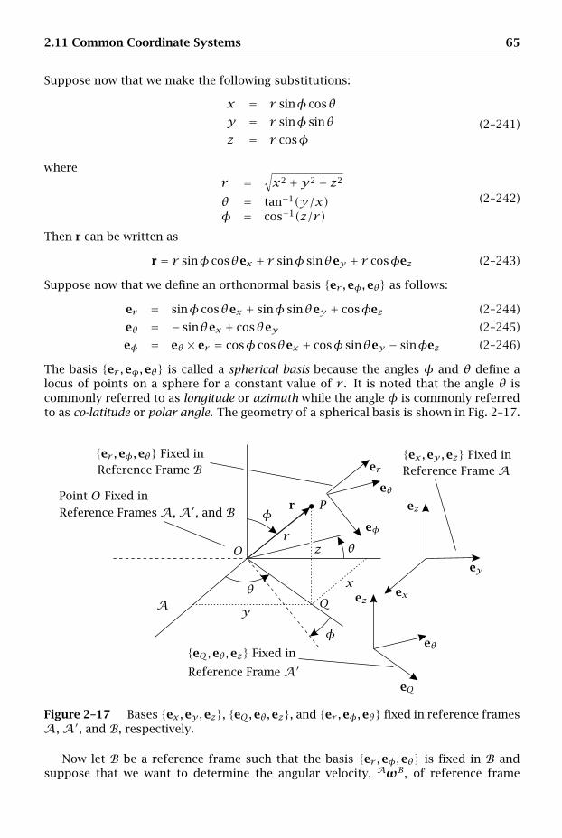
2.11 Common Coordinate Systems 65
Suppose now that we make the following substitutions:
x = r sinφ cosθy = r sinφ sinθz = r cosφ
(2–241)
wherer =
√x2 +y2 + z2
θ = tan−1(y/x)φ = cos−1(z/r)
(2–242)
Then r can be written as
r = r sinφ cosθex + r sinφ sinθey + r cosφez (2–243)
Suppose now that we define an orthonormal basis er ,eφ,eθ as follows:
er = sinφ cosθex + sinφ sinθey + cosφez (2–244)
eθ = − sinθex + cosθey (2–245)
eφ = eθ × er = cosφ cosθex + cosφ sinθey − sinφez (2–246)
The basis er ,eφ,eθ is called a spherical basis because the angles φ and θ define alocus of points on a sphere for a constant value of r . It is noted that the angle θ iscommonly referred to as longitude or azimuth while the angle φ is commonly referredto as co-latitude or polar angle. The geometry of a spherical basis is shown in Fig. 2–17.
Point O Fixed in
A
ex,ey,ez Fixed iner ,eφ,eθ Fixed in
eQ,eθ,ez Fixed in
Reference Frame A
Reference Frames A, A′, and B
Reference Frame A′
Reference Frame B er
eθ
eθ
eφ
eQ
ex
ey
ez
ezr
r
x
y
zO
P
Q
θ
θ
φ
φ
Figure 2–17 Bases ex,ey,ez, eQ,eθ,ez, and er ,eφ,eθ fixed in reference framesA, A′, and B, respectively.
Now let B be a reference frame such that the basis er ,eφ,eθ is fixed in B andsuppose that we want to determine the angular velocity, AωB, of reference frame
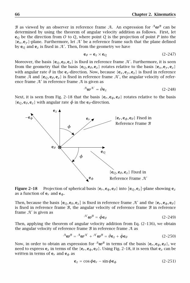
66 Chapter 2. Kinematics
B as viewed by an observer in reference frame A. An expression for AωB can bedetermined by using the theorem of angular velocity addition as follows. First, leteQ be the direction from O to Q, where point Q is the projection of point P into theex,ey-plane. Furthermore, let A′ be a reference frame such that the plane definedby eQ and ez is fixed in A′. Then, from the geometry we have
eθ = ez × eQ (2–247)
Moreover, the basis eQ,eθ,ez is fixed in reference frame A′. Furthermore, it is seenfrom the geometry that the basis eQ,eθ,ez rotates relative to the basis ex,ey,ezwith angular rate θ in the ez-direction. Now, because ex,ey,ez is fixed in referenceframe A and eQ,eθ,ez is fixed in reference frame A′, the angular velocity of refer-ence frame A′ in reference frame A is given as
AωA′ = θez (2–248)
Next, it is seen from Fig. 2–18 that the basis er ,eφ,eθ rotates relative to the basiseQ,eθ,ez with angular rate φ in the eθ-direction.
er ,eφ,eθ Fixed in
eQ,eθ,ez Fixed in
Reference Frame A′
Reference Frame B
⊗
er
eθ
eφ
−eφ
eQ
ez
φ
φ
Figure 2–18 Projection of spherical basis er ,eφ,eθ intoeQ,ez
-plane showing ez
as a function of er and eφ.
Then, because the basiseQ,eθ,ez
is fixed in reference frame A′ and the er ,eφ,eθ
is fixed in reference frame B, the angular velocity of reference frame B in referenceframe A′ is given as
A′ωB = φeθ (2–249)
Then, applying the theorem of angular velocity addition from Eq. (2–136), we obtainthe angular velocity of reference frame B in reference frame A as
AωB = AωA′ + A′ωB = θez + φeθ (2–250)
Now, in order to obtain an expression for AωB in terms of the basis er ,eφ,eθ, weneed to express ez in terms of the er ,eφ,eθ. Using Fig. 2–18, it is seen that ez can bewritten in terms of er and eφ as
ez = cosφer − sinφeφ (2–251)

2.11 Common Coordinate Systems 67
Substituting the result of Eq. (2–251) into (2–250), we obtain AωB as
AωB = θ cosφer − θ sinφeφ + φeθ (2–252)
Using the angular velocity AωB from Eq. (2–252), we can now compute the velocityand acceleration of point P as viewed by an observer in reference frame A. First, thevelocity as viewed by an observer in reference frame A, denoted Av, is obtained fromthe rate of change transport theorem of Eq. (2–128) as
Av =Adrdt
=Bdrdt+AωB × r (2–253)
Using the expression for r and the definition of er from Eqs. (2–243) and (2–244),respectively, we have
r = rer (2–254)
Then, using the expressions for r and AωB from Eqs. (2–254) and (2–252), respectively,we obtain
Bdrdt
= rer (2–255)
AωB × r = (θ cosφer − θ sinφeφ + φeθ)× rer
= rφeφ + r θ sinφeθ (2–256)
Adding the expressions in Eqs. (2–255) and (2–256), we obtain the velocity as viewedby an observer in reference frame A as
Av = rer + rφeφ + r θ sinφeθ (2–257)
Next, applying the rate of change transport theorem of Eq. (2–128) on page 47 to Av,the acceleration of point P as viewed by an observer in reference frame A is obtainedas
Aa =Addt
(Av
)=Bddt
(Av
)+AωB × Av (2–258)
Now we haveBddt
(Av
)= rer + (r φ+ rφ)eφ
+[r θ sinφ+ r(θ sinφ+ φθ cosφ)
]eθ (2–259)
AωB × Av = (θ cosφer − θ sinφeφ + φeθ)
×(rer + rφeφ + r θ sinφeθ)
= rφθ cosφeθ − r θ2 cosφ sinφeφ + r θ sinφeθ
−r θ2 sin2φer + r φeφ − rφ2er
= −(rφ2 + r θ2 sin2φ)er + (r φ− r θ2 cosφ sinφ)eφ+(rφθ cosφ+ r θ sinφ)eθ (2–260)
Adding Eqs. (2–259) and (2–260), we obtain the acceleration as viewed by an observerin reference frame A as
Aa = (r − rφ2 − r θ2 sin2φ)er + (2r φ+ rφ− r θ2 cosφ sinφ)eφ+ (r θ sinφ+ 2rφθ cosφ+ 2r θ sinφ)eθ
(2–261)
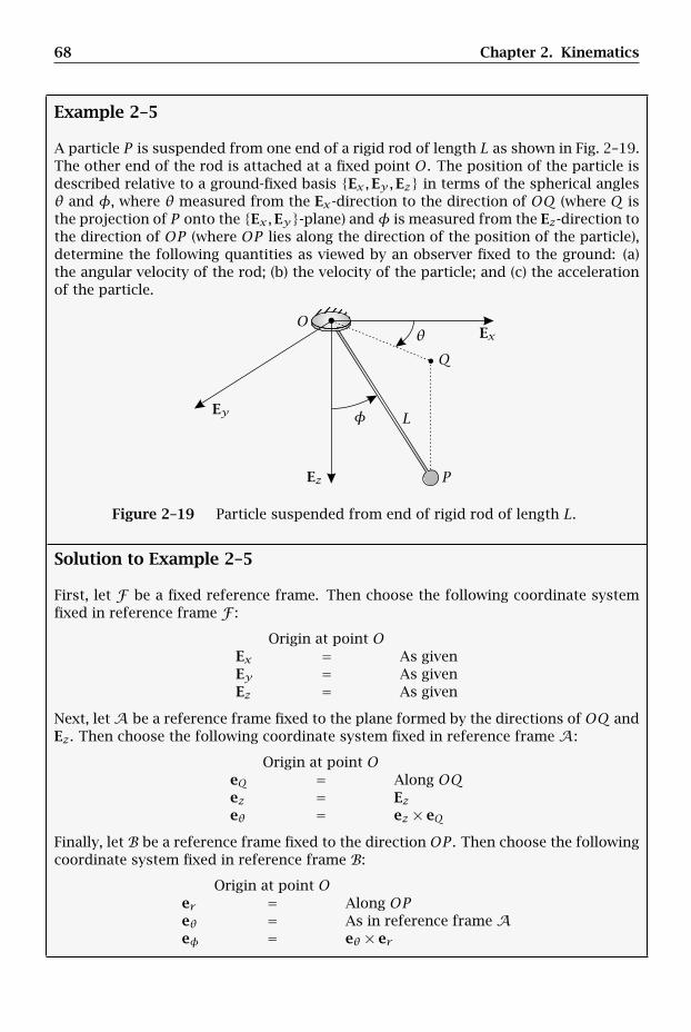
68 Chapter 2. Kinematics
Example 2–5
A particle P is suspended from one end of a rigid rod of length L as shown in Fig. 2–19.The other end of the rod is attached at a fixed point O. The position of the particle isdescribed relative to a ground-fixed basis Ex,Ey,Ez in terms of the spherical anglesθ and φ, where θ measured from the Ex-direction to the direction of OQ (where Q isthe projection of P onto the Ex,Ey-plane) andφ is measured from the Ez-direction tothe direction of OP (where OP lies along the direction of the position of the particle),determine the following quantities as viewed by an observer fixed to the ground: (a)the angular velocity of the rod; (b) the velocity of the particle; and (c) the accelerationof the particle.
Ex
Ey
Ez
L
O
P
Q
θ
φ
Figure 2–19 Particle suspended from end of rigid rod of length L.
Solution to Example 2–5
First, let F be a fixed reference frame. Then choose the following coordinate systemfixed in reference frame F :
Origin at point OEx = As givenEy = As givenEz = As given
Next, letA be a reference frame fixed to the plane formed by the directions of OQ andEz. Then choose the following coordinate system fixed in reference frame A:
Origin at point OeQ = Along OQez = Ezeθ = ez × eQ
Finally, let B be a reference frame fixed to the direction OP . Then choose the followingcoordinate system fixed in reference frame B:
Origin at point Oer = Along OPeθ = As in reference frame Aeφ = eθ × er
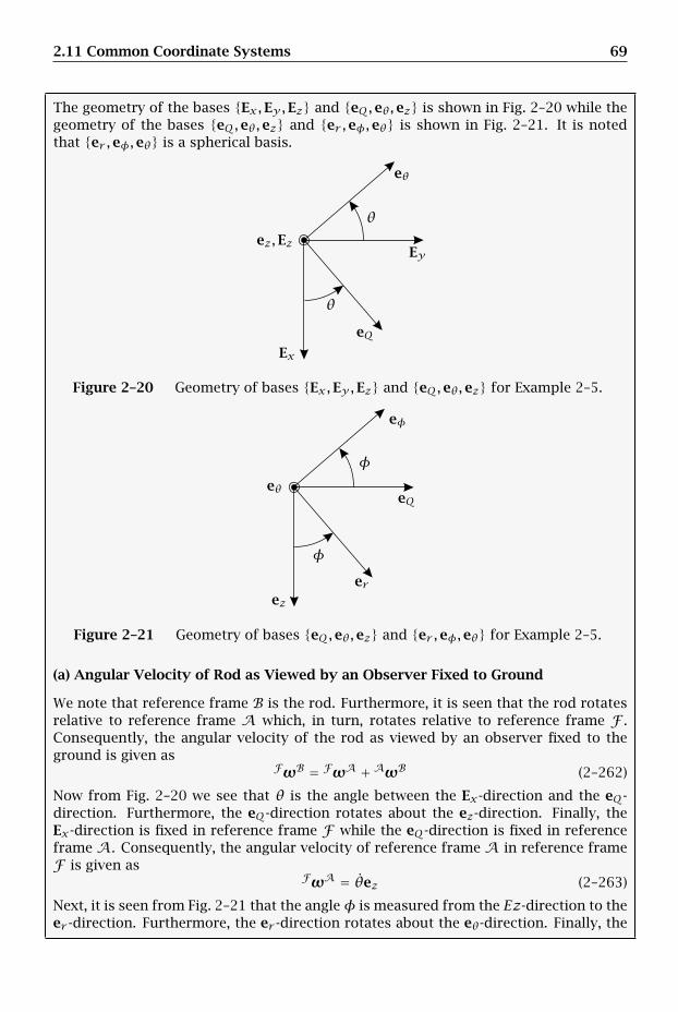
2.11 Common Coordinate Systems 69
The geometry of the bases Ex,Ey,Ez and eQ,eθ,ez is shown in Fig. 2–20 while thegeometry of the bases eQ,eθ,ez and er ,eφ,eθ is shown in Fig. 2–21. It is notedthat er ,eφ,eθ is a spherical basis.
eθ
eQEx
Eyez,Ez
θ
θ
Figure 2–20 Geometry of bases Ex,Ey,Ez and eQ,eθ,ez for Example 2–5.
er
eθ
eφ
eQ
ez
φ
φ
Figure 2–21 Geometry of bases eQ,eθ,ez and er ,eφ,eθ for Example 2–5.
(a) Angular Velocity of Rod as Viewed by an Observer Fixed to Ground
We note that reference frame B is the rod. Furthermore, it is seen that the rod rotatesrelative to reference frame A which, in turn, rotates relative to reference frame F .Consequently, the angular velocity of the rod as viewed by an observer fixed to theground is given as
FωB = FωA +AωB (2–262)
Now from Fig. 2–20 we see that θ is the angle between the Ex-direction and the eQ-direction. Furthermore, the eQ-direction rotates about the ez-direction. Finally, theEx-direction is fixed in reference frame F while the eQ-direction is fixed in referenceframe A. Consequently, the angular velocity of reference frame A in reference frameF is given as
FωA = θez (2–263)
Next, it is seen from Fig. 2–21 that the angleφ is measured from the Ez-direction to theer -direction. Furthermore, the er -direction rotates about the eθ-direction. Finally, the

70 Chapter 2. Kinematics
Ez-direction is fixed in reference frame A while the er -direction is fixed in referenceframe B. Consequently, the angular velocity of reference frame A in reference frameF is given as
AωB = φeθ (2–264)
Applying the angular velocity addition theorem of Eq. (2–136) on page 48 using theangular velocities given in Eqs. (2–263) and (2–264), we obtain the angular velocity ofreference frame B in reference frame F as
FωB = θez + φeθ (2–265)
Now it is seen that the expression for FωB is given in terms of both the basiseQ,eθ,ez (where eQ,eθ,ez is fixed in reference frame A) and the basis er ,eφ,eθ(where er ,eφ,eθ is fixed in reference frame B). In order to obtain an expressionpurely in terms of the basis er ,eφ,eθ, we need to express ez in terms of the basiser ,eφ,eθ. Using Fig. 2–21), we obtain the following expression for ez in terms of thebasis er ,eφ,eθ:
ez = cosφer − sinφeφ (2–266)
Substituting the expression for ez from Eq. (2–266) into (2–265), we obtain
FωB = θ(cosφer − sinφeφ)+ φeθ (2–267)
Rearranging Eq. (2–267), we obtain the angular velocity of the rod as viewed by anobserver fixed to the ground as
FωB = θ cosφer − θ sinφeφ + φeθ (2–268)
(b) Velocity of Particle as Viewed by an Observer Fixed to Ground
Because er is the direction from O to P , the position of the particle is given as
r = Ler (2–269)
The velocity of the particle as viewed by an observer fixed to the ground is then ob-tained from the rate of change transport theorem of Eq. (2–128) on page 47 as
Fv =Fdrdt
=Bdrdt+ FωB × r (2–270)
Using the expressions for r and FωB from Eqs. (2–269) and (2–268), respectively, wehave
Bdrdt
= 0 (2–271)
FωB × r = (θ cosφer − θ sinφeφ + φeθ)× Ler (2–272)
Expanding Eq. (2–272), we obtain
FωB × r = Lθ sinφeθ + Lφeφ = Lφeφ + Lθ sinφeθ (2–273)
Adding Eqs. (2–271) and (2–273), we obtain the velocity of the particle as viewed by anobserver fixed to the ground as
Fv = Lφeφ + Lθ sinφeθ (2–274)
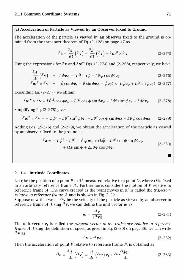
2.11 Common Coordinate Systems 71
(c) Acceleration of Particle as Viewed by an Observer Fixed to Ground
The acceleration of the particle as viewed by an observer fixed to the ground is ob-tained from the transport theorem of Eq. (2–128) on page 47 as
Fa =Fddt
(Fv)=Bddt
(Fv)+ FωB × Fv (2–275)
Using the expressions for Fv and FωB Eqs. (2–274) and (2–268), respectively, we have
Bddt
(Fv)
= Lφeφ + (Lθ sinφ+ Lθφ cosφ)eθ (2–276)
FωB × Fv = (θ cosφer − θ sinφeφ + φeθ)× (Lφeφ + Lθ sinφeθ) (2–277)
Expanding Eq. (2–277), we obtain
FωB × Fv = Lθφ cosφeθ − Lθ2 cosφ sinφeφ − Lθ2 sin2φer − Lφ2er (2–278)
Simplifying Eq. (2–278) gives
FωB × Fv = −(Lφ2 + Lθ2 sin2φ)er − Lθ2 cosφ sinφeφ + Lθφ cosφeθ (2–279)
Adding Eqs. (2–276) and (2–279), we obtain the acceleration of the particle as viewedby an observer fixed to the ground as
Fa = −(Lφ2 + Lθ2 sin2φ)er + (Lφ− Lθ2 cosφ sinφ)eφ+ (Lθ sinφ+ 2Lθφ cosφ)eθ
(2–280)
2.11.4 Intrinsic Coordinates
Let r be the position of a point P in R3 measured relative to a point O, where O is fixedin an arbitrary reference frame A. Furthermore, consider the motion of P relative toreference frame A. The curve created as the point moves in R3 is called the trajectoryrelative to reference frame A and is shown in Fig. 2–22.Suppose now that we let Av be the velocity of the particle as viewed by an observer inreference frame A. Using Av, we can define the unit vector et as
et =Av‖Av‖ (2–281)
The unit vector et is called the tangent vector to the trajectory relative to referenceframe A. Using the definition of speed as given in Eq. (2–30) on page 36, we can writeAv as
Av = Avet (2–282)
Then the acceleration of point P relative to reference frame A is obtained as
Aa =Addt
(Av
)= ddt
(Av
)et +Av
Adetdt
(2–283)
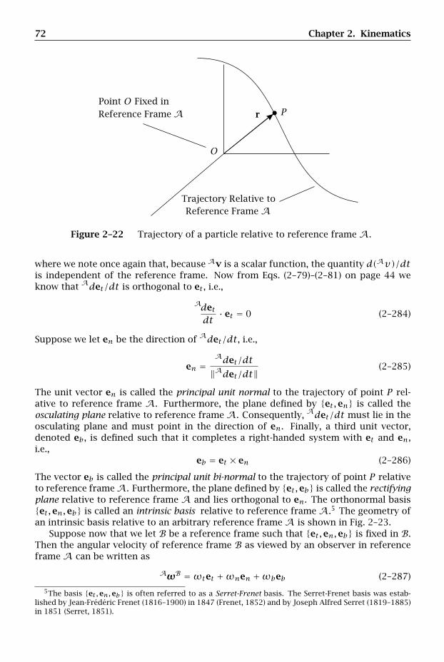
72 Chapter 2. Kinematics
Point O Fixed in
Trajectory Relative to
Reference Frame A
Reference Frame A
r
O
P
Figure 2–22 Trajectory of a particle relative to reference frame A.
where we note once again that, because Av is a scalar function, the quantity d(Av)/dtis independent of the reference frame. Now from Eqs. (2–79)–(2–81) on page 44 weknow that Adet/dt is orthogonal to et , i.e.,
Adetdt
· et = 0 (2–284)
Suppose we let en be the direction of Adet/dt, i.e.,
en =Adet/dt‖Adet/dt‖
(2–285)
The unit vector en is called the principal unit normal to the trajectory of point P rel-ative to reference frame A. Furthermore, the plane defined by et,en is called theosculating plane relative to reference frame A. Consequently, Adet/dt must lie in theosculating plane and must point in the direction of en. Finally, a third unit vector,denoted eb, is defined such that it completes a right-handed system with et and en,i.e.,
eb = et × en (2–286)
The vector eb is called the principal unit bi-normal to the trajectory of point P relativeto reference frameA. Furthermore, the plane defined by et,eb is called the rectifyingplane relative to reference frame A and lies orthogonal to en. The orthonormal basiset,en,eb is called an intrinsic basis relative to reference frame A.5 The geometry ofan intrinsic basis relative to an arbitrary reference frame A is shown in Fig. 2–23.
Suppose now that we let B be a reference frame such that et,en,eb is fixed in B.Then the angular velocity of reference frame B as viewed by an observer in referenceframe A can be written as
AωB =ωtet +ωnen +ωbeb (2–287)
5The basis et ,en,eb is often referred to as a Serret-Frenet basis. The Serret-Frenet basis was estab-lished by Jean-Frederic Frenet (1816–1900) in 1847 (Frenet, 1852) and by Joseph Alfred Serret (1819–1885)in 1851 (Serret, 1851).
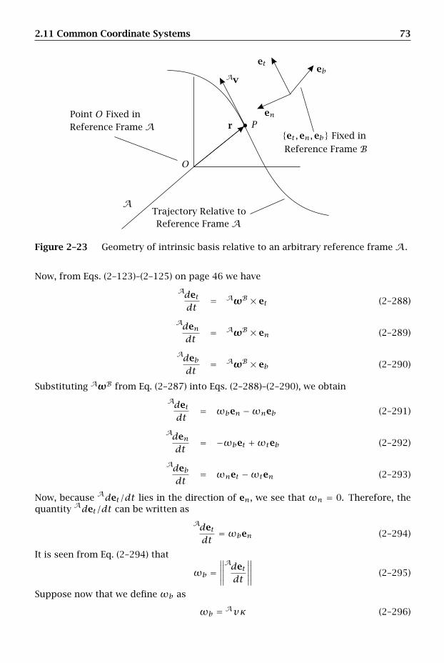
2.11 Common Coordinate Systems 73
Point O Fixed in
Av
A
et,en,eb Fixed in
Trajectory Relative toReference Frame A
Reference Frame A
Reference Frame B
et
en
eb
r
O
P
Figure 2–23 Geometry of intrinsic basis relative to an arbitrary reference frame A.
Now, from Eqs. (2–123)–(2–125) on page 46 we have
Adetdt
= AωB × et (2–288)
Adendt
= AωB × en (2–289)
Adebdt
= AωB × eb (2–290)
Substituting AωB from Eq. (2–287) into Eqs. (2–288)–(2–290), we obtain
Adetdt
= ωben −ωneb (2–291)
Adendt
= −ωbet +ωteb (2–292)
Adebdt
= ωnet −ωten (2–293)
Now, because Adet/dt lies in the direction of en, we see that ωn = 0. Therefore, thequantity Adet/dt can be written as
Adetdt
=ωben (2–294)
It is seen from Eq. (2–294) that
ωb =∥∥∥∥∥Adetdt
∥∥∥∥∥ (2–295)
Suppose now that we define ωb as
ωb = Avκ (2–296)
74 Chapter 2. Kinematics
Then, because ωn = 0, from Eq. (2–291) we have
Adetdt
= Avκen (2–297)
The quantity κ ≥ 0 is called the curvature of the path of the particle as viewed by anobserver in reference frame A. Furthermore, because ωn = 0, we have from Eq. (2–293) that
Adebdt
= −ωten (2–298)
Furthermore, suppose we letωt = Avτ (2–299)
The quantity τ is called the torsion of the path of the particle as viewed by an observerin reference frame A. Then Adeb/dt can be written as
Adebdt
= −Avτen (2–300)
Using ωb from Eq. (2–296) and ωt from Eq. (2–299), we obtain
Adendt
= −Avκet +Avτeb (2–301)
We then obtain AωB asAωB = Av(τet + κeb) (2–302)
Consequently, the rates of change of the vectors et , en, and eb relative to referenceframe A are given from Eqs. (2–297), (2–301), and (2–300), respectively, as
Adetdt
= Avκen (2–303)
Adendt
= −Avκet +Avτeb (2–304)
Adebdt
= −Avτen (2–305)
We see from Eqs. (2–303)–(2–305) that the curvature and torsion are given as
κ = 1Av
∥∥∥∥∥Adetdt
∥∥∥∥∥ (2–306)
τ = 1Av
∥∥∥∥∥Adebdt
∥∥∥∥∥ (2–307)
Finally, substituting the expression for Adet/dt from Eq. (2–297) into (2–283), we ob-tain the acceleration of the particle at point P as
Aa = ddt
(Av
)et + κ
(Av
)2en (2–308)
While for many applications it is most convenient to use time as the independentvariable, for some problems it is more convenient to think of the trajectory relative to a
2.11 Common Coordinate Systems 75
reference frame A as spatial rather than temporal. For such problems it is convenientto use the arc-length, As, as defined in Eq. (2–32) on page 36, as the independentvariable. Suppose for convenience that we let
s = As (2–309)
Then, applying the chain rule using Eq. (2–309), the rates of change of et , en, and ebwith respect to s are given, respectively, as
Adetds
=Adetdtdtds
(2–310)
Adends
=Adendt
dtds
(2–311)
Adebds
=Adebdtdtds
(2–312)
Furthermore, using ds/dt from Eq. (2–32) on page 36, we have
dtds
= 1Av
(2–313)
Substituting the expression for dt/ds from Eq. (2–313) into Eqs. (2–303)–(2–305), weobtain the quantities Adet/ds, Aden/ds, and Adeb/ds, respectively, as
Adetds
= κen (2–314)
Adends
= −κet + τeb (2–315)
Adebds
= −τen (2–316)
Equations (2–314)–(2–316) are called the Serret-Frenet formulas (Serret, 1851; Frenet,1852) and describe the spatial rate of change of the intrinsic basis et,en,eb. FromEqs. (2–314)–(2–316), the curvature and torsion are given as
κ =∥∥∥∥∥Adetds
∥∥∥∥∥ (2–317)
τ =∥∥∥∥∥Adebds
∥∥∥∥∥ (2–318)
Finally, we can define the Darboux vector, AωBSF , as
AωBSF =
AωBAv
= τet + κeb (2–319)
In terms of the Darboux vector, the Serret-Frenet formulas can be written as
Adetds
= AωBSF × et (2–320)
Adends
= AωBSF × en (2–321)
Adebds
= AωBSF × eb (2–322)

76 Chapter 2. Kinematics
We note that the acceleration of Eq. (2–308) is the same regardless of whether wechoose a temporal or spatial description of the trajectory of point P .
It is important to understand a fundamental difference between intrinsic coordi-nates and other commonly used coordinate systems. In other commonly used coor-dinate systems (e.g., Cartesian, cylindrical, or spherical coordinates) the basis is usedto describe the position of the particle. However, it is seen that intrinsic coordinatesdo not describe position, but instead describe motion along velocity (i.e., motion alonget) and motion orthogonal to velocity (i.e., motion along en and eb). Consequently,in general it is not possible to start with an expression for position in terms of anintrinsic basis and then determine velocity and acceleration using this expression forposition. Instead, when using intrinsic coordinates it is necessary to define position interms of some other coordinate system and then define the intrinsic basis in terms ofthis other coordinate system. As a result, it is generally not possible to use intrinsiccoordinates alone; a second (auxiliary) coordinate system must be used in conjunctionwith intrinsic coordinates.
Example 2–6
A particle moves along a curve in the form of a fixed circular track. The equation forthe track is given as
r = sinθ
Assuming the initial conditions θ(t = 0) = 0 and θ(t = 0) = θ0, determine (a) thearc-length parameter s as a function of the angle θ; (b) the intrinsic basis et,en,ebin terms of a cylindrical basis fixed to the motion of the particle; (c) the curvature ofthe trajectory; and (d) the position, velocity, and acceleration of the particle in termsof the intrinsic basis et,en,eb.
Ex
Ey
r
O
P
θ
Figure 2–24 Particle moving on a circle.
Solution to Example 2–6
First, let F be a reference frame fixed to the circular track. Then choose the following
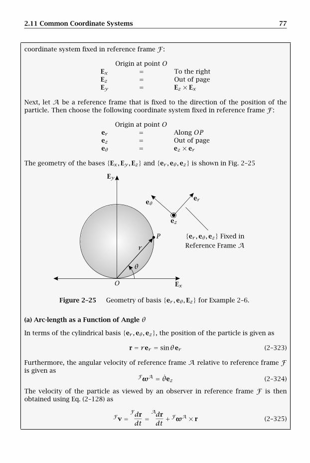
2.11 Common Coordinate Systems 77
coordinate system fixed in reference frame F :
Origin at point OEx = To the rightEz = Out of pageEy = Ez × Ex
Next, let A be a reference frame that is fixed to the direction of the position of theparticle. Then choose the following coordinate system fixed in reference frame F :
Origin at point Oer = Along OPez = Out of pageeθ = ez × er
The geometry of the bases Ex,Ey,Ez and er ,eθ,ez is shown in Fig. 2–25
er ,eθ,ez Fixed in
Reference Frame A
ereθ
ez
Ex
Ey
r
O
P
θ
Figure 2–25 Geometry of basis er ,eθ,Ez for Example 2–6.
(a) Arc-length as a Function of Angle θ
In terms of the cylindrical basis er ,eθ,ez, the position of the particle is given as
r = rer = sinθer (2–323)
Furthermore, the angular velocity of reference frame A relative to reference frame Fis given as
FωA = θez (2–324)
The velocity of the particle as viewed by an observer in reference frame F is thenobtained using Eq. (2–128) as
Fv =Fdrdt
=Adrdt+ FωA × r (2–325)
78 Chapter 2. Kinematics
Now we have
Adrdt
= θ cosθer (2–326)
FωA × r = θez × sinθer = θ sinθeθ (2–327)
Adding the expressions in Eqs. (2–326) and (2–327), we obtain the velocity of the par-ticle in reference frame F as
Fv = θ cosθer + θ sinθeθ = θ(cosθer + sinθeθ) (2–328)
The speed of the particle as viewed by an observer in reference frame F is then givenas
Fv = ‖Fv‖ = ‖θ(cosθer + sinθeθ)‖ = θ (2–329)
The arc-length parameter in reference frame F is then obtained from Eq. (2–32) onpage 36 as
ddt
(Fs)= Fv = θ = dθ
dt(2–330)
Setting Fs = s, we have from Eq. (2–330) that
ds = dθ (2–331)
Integrating both sides of Eq. (2–6), we obtain
∫ ss0du =
∫ θθ0
du (2–332)
where u is a dummy variable of integration. Then, using the initial conditions θ(t =0) = 0 and s0 = 0, we obtain the arc-length parameter in terms of θ as
s ≡ Fs = θ (2–333)
(b) Intrinsic Basis in Terms of Cylindrical Basis
The tangent vector et is obtained using the velocity from Eq. (2–328) and the speedfrom Eq. (2–329) as
et =FvFv
= cosθer + sinθeθ (2–334)
The rate of change of et in reference frame F is then obtained from the transporttheorem of Eq. (2–128) on page 47 as
Fdetdt
=Adetdt
+ FωA × et (2–335)
where
Adetdt
= −θ sinθer + θ cosθeθ (2–336)
FωA × et = θez × (cosθer + sinθeθ)= −θ sinθer + θ cosθeθ (2–337)
2.11 Common Coordinate Systems 79
Adding the expressions in Eqs. (2–336) and (2–337), we obtain
Fdetdt
= −2θ sinθer + 2θ cosθeθ (2–338)
Then, using Eq. (2–285), we have
en =Fdet/dt∥∥∥Fdet/dt
∥∥∥ (2–339)
Substituting Fdet/dt from Eq. (2–338) into (2–339), we obtain
en = −2θ sinθer + 2θ cosθeθ2θ
= − sinθer + cosθeθ (2–340)
Finally, the vector eb is obtained from the right-hand rule as
eb = et × en = (cosθer + sinθeθ)× (− sinθer + cosθeθ) = ez (2–341)
(c) Curvature of Trajectory
From Eq. (2–303) we haveFdetdt
= Fvκen (2–342)
Consequently, the curvature of the trajectory is given as
κ = ‖Fdet/dt‖Fv
= 2θθ= 2 (2–343)
(d) Position, Velocity, and Acceleration of Particle in Terms of Intrinsic Basis
The position was given earlier in terms of the cylindrical basis as
r = sinθer (2–344)
Now, from Eqs. (2–334) and (2–339) we have
et = cosθer + sinθeθen = − sinθer + cosθeθ
(2–345)
Solving Eq. (2–345) for er , we obtain
er = cosθet − sinθen (2–346)
Consequently, the position of the particle is given in the intrinsic basis et,en,eb as
r = sinθ(cosθet − sinθen) = sinθ cosθet − sin2θen (2–347)
Then, from Eq. (2–282) we obtain Fv in terms of the intrinsic basis as
Fv = Fvet = θet (2–348)
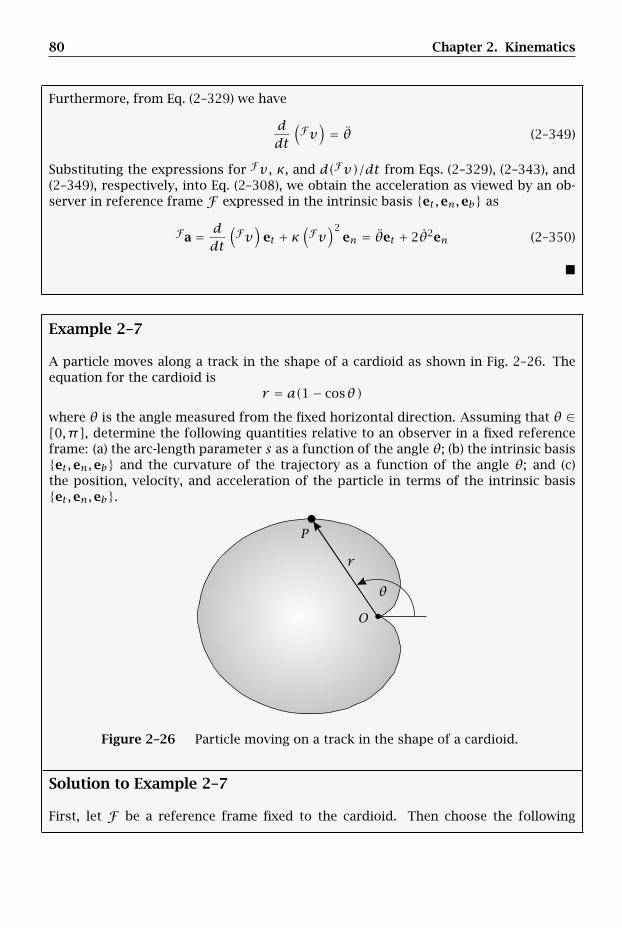
80 Chapter 2. Kinematics
Furthermore, from Eq. (2–329) we have
ddt
(Fv
)= θ (2–349)
Substituting the expressions for Fv , κ, and d(Fv)/dt from Eqs. (2–329), (2–343), and(2–349), respectively, into Eq. (2–308), we obtain the acceleration as viewed by an ob-server in reference frame F expressed in the intrinsic basis et,en,eb as
Fa = ddt
(Fv
)et + κ
(Fv
)2en = θet + 2θ2en (2–350)
Example 2–7
A particle moves along a track in the shape of a cardioid as shown in Fig. 2–26. Theequation for the cardioid is
r = a(1− cosθ)
where θ is the angle measured from the fixed horizontal direction. Assuming that θ ∈[0, π], determine the following quantities relative to an observer in a fixed referenceframe: (a) the arc-length parameter s as a function of the angle θ; (b) the intrinsic basiset,en,eb and the curvature of the trajectory as a function of the angle θ; and (c)the position, velocity, and acceleration of the particle in terms of the intrinsic basiset,en,eb.
r
O
P
θ
Figure 2–26 Particle moving on a track in the shape of a cardioid.
Solution to Example 2–7
First, let F be a reference frame fixed to the cardioid. Then choose the following
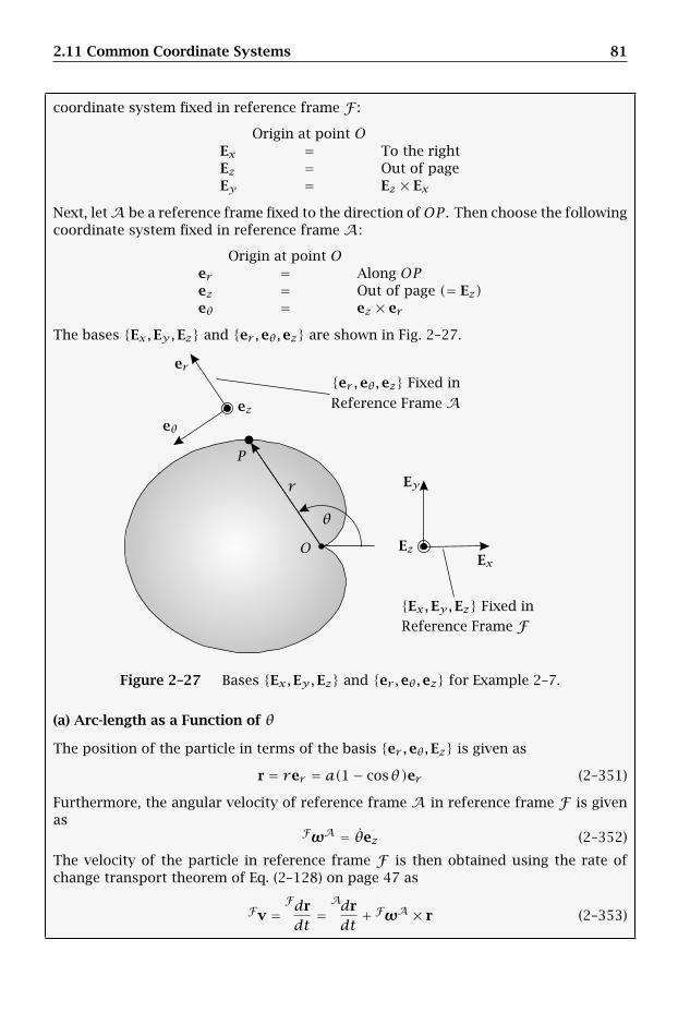
2.11 Common Coordinate Systems 81
coordinate system fixed in reference frame F :
Origin at point OEx = To the rightEz = Out of pageEy = Ez × Ex
Next, letA be a reference frame fixed to the direction ofOP . Then choose the followingcoordinate system fixed in reference frame A:
Origin at point Oer = Along OPez = Out of page (= Ez)eθ = ez × er
The bases Ex,Ey,Ez and er ,eθ,ez are shown in Fig. 2–27.
Ex,Ey,Ez Fixed in
er ,eθ,ez Fixed in
Reference Frame A
Reference Frame F
er
eθ
ez
Ex
Ey
Ez
r
O
P
θ
Figure 2–27 Bases Ex,Ey,Ez and er ,eθ,ez for Example 2–7.
(a) Arc-length as a Function of θ
The position of the particle in terms of the basis er ,eθ,Ez is given as
r = rer = a(1− cosθ)er (2–351)
Furthermore, the angular velocity of reference frame A in reference frame F is givenas
FωA = θez (2–352)
The velocity of the particle in reference frame F is then obtained using the rate ofchange transport theorem of Eq. (2–128) on page 47 as
Fv =Fdrdt
=Adrdt+ FωA × r (2–353)
82 Chapter 2. Kinematics
Now we have
Adrdt
= rer = aθ sinθer (2–354)
FωA × r = θez × a(1− cosθ)er = a(1− cosθ)θeθ (2–355)
Adding Eqs. (2–354) and (2–355), the velocity of the particle in reference frame F isobtained as
Fv = aθ sinθer + a(1− cosθ)θeθ (2–356)
Equation (2–356) can be rewritten as
Fv = aθ [sinθer + (1− cosθ)eθ] (2–357)
The speed of the particle in reference frame F is then obtained from Eq. (2–357) as
Fv = ‖Fv‖ = aθ[sin2θ + (1− cosθ)2
]1/2(2–358)
Expanding Eq. (2–358), we obtain
Fv = aθ[sin2θ + 1− 2 cosθ + cos2θ
]1/2(2–359)
Noting that sin2θ + cos2θ = 1, Eq. (2–359) can be simplified to
Fv = aθ√
2 [1− cosθ]1/2 (2–360)
Now from trigonometry we have
1− cosθ = 2 sin2 (θ/2) (2–361)
Substituting the result from Eq. (2–361) into (2–360), we obtain
Fv = 2aθ sin (θ/2) (2–362)
Then, using the expression for arc-length from
ddt
(Fs)= Fv = 2aθ sin (θ/2) (2–363)
Setting s = Fs, Eq. (2–363) can be written as
dsdθ
= 2a sin (θ/2) (2–364)
Separating the variables s and θ in Eq. (2–364) gives
ds = 2a sin (θ/2)dθ (2–365)
Integrating both sides of Eq. (2–365), we obtain
∫ ss0du =
∫ θθ0
2a sin (u/2)du (2–366)
2.11 Common Coordinate Systems 83
Consequently,s − s0 = [−4a cos (θ/2)]θθ0
(2–367)
Equation (2–367) can then be written as
s − s0 = −4a[cos (θ/2)− cos (θ0/2)] (2–368)
Finally, using the initial condition θ(t = 0) = 0, we have s0 = 0. from which Eq. (2–368)reduces to
s ≡ Fs = −4a[cos (θ/2)− 1] (2–369)
The arc-length in reference frame F is then given in terms of θ as
Fs = 4a[1− cos (θ/2)] (2–370)
(b) Determination of Intrinsic Basis
First, the tangent vector in reference frame F is given as
et =FvFv
(2–371)
Then, using Fv from Eq. (2–357) and Fv from Eq. (2–362), we obtain the tangent vector
et = aθ [sinθer + (1− cosθ)eθ]2aθ sin (θ/2)
(2–372)
Separating the er and eθ components in Eq. (2–372) gives
et = sinθ2 sin (θ/2)
er + 1− cosθ2 sin (θ/2)
eθ (2–373)
Now from trigonometry we have
sinθ = 2 sin (θ/2) cos (θ/2) (2–374)
Substituting Eq. (2–374) and the earlier trigonometric identity from Eq. (2–361) into(2–373), we obtain
et = 2 sin (θ/2) cos (θ/2)2 sin (θ/2)
er + 2 sin2 (θ/2)2 sin (θ/2)
eθ (2–375)
Canceling out the common factor of sin (θ/2) from the numerator and denominatorof each term in Eq. (2–375), we obtain the tangent vector
et = cos (θ/2)er + sin (θ/2)eθ (2–376)
Next, from the Serret-Frenet formulas we have
Fdetdt
= Fvκen (2–377)
84 Chapter 2. Kinematics
Computing the rate of change of et in reference frame F , we have
Fdetdt
=Adetdt
+ FωA × et (2–378)
Now we have
Adetdt
= −12 θ sin (θ/2)er + 1
2 θ cos (θ/2)eθ (2–379)
FωA × et = θez × [cos (θ/2)er + sin (θ/2)eθ]= −θ sin (θ/2)er + θ cos (θ/2)eθ (2–380)
Adding the expressions in Eqs. (2–379) and (2–380), we obtain
Fdetdt
= −32 θ sin (θ/2)er + 3
2 θ cos (θ/2)eθ (2–381)
It can be seen from Eq. (2–381) that∥∥∥∥∥Fdetdt
∥∥∥∥∥ = 32 θ = Fvκ (2–382)
Then, using Fv from Eq. (2–362), we obtain κ as
κ = 3θ/22aθ sin (θ/2)
= 34a sin (θ/2)
(2–383)
Now, because en =(Fdet/dt
)/‖det/dt‖, we obtain en as
en = − sin (θ/2)er + cos (θ/2)eθ (2–384)
Finally, the principal unit bi-normal vector is computed using et from Eq. (2–376) anden from Eq. (2–384) as
eb = et × en= [cos (θ/2)er + sin (θ/2)eθ]× [− sin (θ/2)er + cos (θ/2)eθ]= ez
(2–385)
(c) Position, Velocity, and Acceleration of Particle in Terms of Intrinsic Basis
First, in order to express r (as given in Eq. (2–351)) in terms of et,en,eb, it is neces-sary to solve for er in terms of et,en,eb. We have from Eqs. (2–376) and (2–384)
et = cos (θ/2)er + sin (θ/2)eθ (2–386)
en = − sin (θ/2)er + cos (θ/2)eθ (2–387)
Multiplying Eq. (2–386) and (2–387) by cos (θ/2) and sin (θ/2), respectively, and sub-tracting gives
cos (θ/2)et − sin (θ/2)en = cos2 (θ/2)er + sin2 (θ/2)er = er (2–388)
2.12 Kinematics in a Rotating and Translating Reference Frame 85
Substituting er from Eq. (2–388) into (2–351), the position of the particle is obtainedin terms of the intrinsic basis et,en,eb as
r = a(1− cosθ) [cos (θ/2)et − sin (θ/2)en] (2–389)
Now the velocity in reference frame F is obtained using the speed in Eq. (2–362) as
Fv = Fvet = 2aθ sin (θ/2)et (2–390)
The acceleration in reference frameF is given in terms of the intrinsic basis et,en,ebas
Fa = ddt
(Fv
)et + κ
(Fv
)2en (2–391)
Differentiating Fv in Eq. (2–362), we obtain
ddt
(Fv
)= 2aθ sin (θ/2)+ aθ2 cos (θ/2) (2–392)
Next, computing κ(Fv)2
using κ from Eq. (2–383), we obtain
κ(Fv
)2 = 34a sin (θ/2)
[2aθ sin (θ/2)
]2 = 3aθ2 sin (θ/2) (2–393)
Substituting the results of Eqs. (2–392) and (2–393) into Eq. (2–391), the accelerationof the particle in given in terms of the intrinsic basis as
Fa =[2aθ sin (θ/2)+ aθ2 cos (θ/2)
]et + 3aθ2 sin (θ/2)en (2–394)
2.12 Kinematics in a Rotating and Translating Reference Frame
In many dynamics problems it is most convenient to describe the motion of a pointusing a reference frame that both translates and rotates relative to another referenceframe. In this Section we describe the kinematics of a particle using a rotating andtranslating reference frame.
Let A and B be two reference frames such that B rotates and translates relative toA. Furthermore, let O be a point fixed in A and let Q be a point fixed in B. Then, letrQ be the position of a point Q relative to a point O and let rP/Q be the position of apoint P relative to point Q. Finally, let AωB be the angular velocity of reference frameB as viewed by an observer in reference frame A. The points O, Q, and P and thereference frames A and B are shown in Fig. 2–28, where it can be seen that referenceframe B simultaneously rotates and translates relative to reference frame A. UsingFig. 2–28, the position of point P relative to point O can then be written as
rP = rQ + rP/Q (2–395)
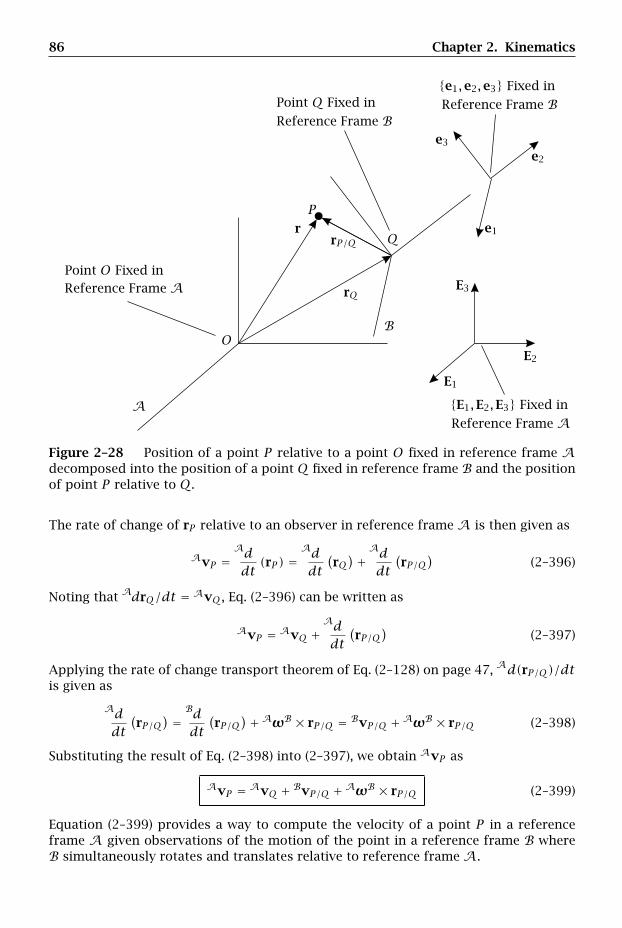
86 Chapter 2. Kinematics
Point O Fixed in
Point Q Fixed in
A
e1,e2,e3 Fixed in
E1,E2,E3 Fixed in
Reference Frame A
Reference Frame A
Reference Frame BReference Frame B
e1
e2
e3
E1
E2
E3
r
rQ
rP/Q
O
P
Q
B
Figure 2–28 Position of a point P relative to a point O fixed in reference frame Adecomposed into the position of a point Q fixed in reference frame B and the positionof point P relative to Q.
The rate of change of rP relative to an observer in reference frame A is then given as
AvP =Addt(rP ) =
Addt
(rQ)+Ad
dt(rP/Q
)(2–396)
Noting that AdrQ/dt = AvQ, Eq. (2–396) can be written as
AvP = AvQ +Addt
(rP/Q
)(2–397)
Applying the rate of change transport theorem of Eq. (2–128) on page 47, Ad(rP/Q)/dtis given as
Addt
(rP/Q
) = Bddt
(rP/Q
)+AωB × rP/Q = BvP/Q +AωB × rP/Q (2–398)
Substituting the result of Eq. (2–398) into (2–397), we obtain AvP as
AvP = AvQ + BvP/Q +AωB × rP/Q (2–399)
Equation (2–399) provides a way to compute the velocity of a point P in a referenceframe A given observations of the motion of the point in a reference frame B whereB simultaneously rotates and translates relative to reference frame A.

2.12 Kinematics in a Rotating and Translating Reference Frame 87
Using the expression for AvP from Eq. (2–399), the acceleration of point P in refer-ence frame A is obtained as
AaP =Addt
(AvP
)=Addt
(AvQ + BvP/Q +AωB × rP/Q
)(2–400)
Expanding Eq. (2–400) gives
AaP =Addt
(AvQ
)+Addt
(BvP/Q
)+Addt
(AωB × rP/Q
)(2–401)
Now we note thatAddt
(AvQ
)= AaQ (2–402)
where AaQ is the acceleration of point Q in reference frame A. Furthermore, from therate of change transport theorem of Eq. (2–128) on page 47, we have
Addt
(BvP/Q
)=Bddt
(BvP/Q
)+AωB × BvP/Q (2–403)
Now we note thatBddt
(BvP/Q
)= BaP/Q (2–404)
Consequently, Eq. (2–401) can be written as
AaP = AaQ + BaP/Q +AωB × BvP/Q +Addt
(AωB × rP/Q
)(2–405)
Next, we have
Addt
(AωB × rP/Q
)=Addt
(AωB
)× rP/Q +AωB ×
Addt
(rP/Q
)(2–406)
Now, we know thatAddt
(AωB
)= AαB
Addt
(rP/Q
) = AvP/Q
(2–407)
Therefore, Eq. (2–406) can be written as
Addt
(AωB × rP/Q
)= AαB × rP/Q +AωB × AvP/Q (2–408)
Furthermore, we have from the rate of change transport theorem that
AvP/Q =Addt
(rP/Q
) = Bddt
(rP/Q
)+AωB × rP/Q = BvP/Q +AωB × rP/Q (2–409)
Substituting the result of Eq. (2–409) into (2–408), we have
Addt
(AωB × rP/Q
)= AαB × rP/Q +AωB ×
(BvP/Q +AωB × rP/Q
)= AαB × rP/Q +AωB × BvP/Q +AωB ×
(AωB × rP/Q
) (2–410)
88 Chapter 2. Kinematics
Then, substituting the expression from Eq. (2–410) into (2–405), we obtain
AaP = AaQ + BaP/Q +AωB × BvP/Q
+AαB × rP/Q +AωB × BvP/Q +AωB ×(AωB × rP/Q
) (2–411)
Equation (2–411) simplifies to
AaP = AaQ + BaP/Q +AαB × rP/Q
+ 2AωB × BvP/Q +AωB ×(AωB × rP/Q
) (2–412)
Equation (2–412) provides a way to compute the acceleration of a point P in a referenceframe A given observations of the motion of the point in a reference frame B, whereB simultaneously rotates and translates relative to reference frame A. It is notedthat, for historical reasons, the third, fourth, and fifth terms in Eq. (2–412) have thefollowing names:
AαB × rP/Q = Euler acceleration
2AωB × BvP/Q = Coriolis acceleration
AωB × (AωB × rP/Q) = Centripetal acceleration
2.13 Practical Approach to Computing Velocity and Acceleration
In Sections 2.9 and 2.12 we derived expressions for the velocity and acceleration of apoint in a reference frame A given observations about the motion of the point in areference frame B, where reference frame B either rotates, or rotates and translates,relative to reference frame A. While in principle these results can be used directly tocompute velocity and acceleration, in practice it is often difficult to implement theseresults because it is necessary to keep track of many quantities simultaneously.6 Con-sequently, unless one has a complete understanding of each term in these equations,it is preferable to start at a more fundamental level and apply the rate of changetransport theorem of Eq. (2–128) twice. More specifically, the rate of change transporttheorem is first applied to position to obtain velocity and is applied a second time tovelocity to obtain acceleration. While two applications of the rate of change transporttheorem are less direct than a single application of either Eq. (2–158) in Section 2.9 orEq. (2–412) in Section 2.12, using a two-step approach is more straightforward, therebyminimizing the possibility for error.
Example 2–8
Two rigid rods of lengths l1 and l2 are hinged in tandem as shown in Fig. 2–29. RodOA is hinged at one of its ends to the fixed point O while its other end is hinged atpoint A, where A is one end of the second rod AP . Point P is located at the free end ofrod AP . Knowing that θ is the angle between rod OA and the horizontal and that φ is
6It is particularly difficult to implement the results for acceleration as given in Eqs. (2–158) and (2–412).
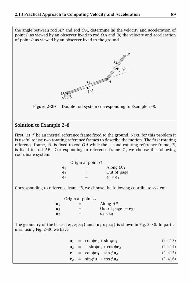
2.13 Practical Approach to Computing Velocity and Acceleration 89
the angle between rod AP and rod OA, determine (a) the velocity and acceleration ofpoint P as viewed by an observer fixed to rod OA and (b) the velocity and accelerationof point P as viewed by an observer fixed to the ground.
l1
l2
A
O
P
θ
φ
Figure 2–29 Double rod system corresponding to Example 2–8.
Solution to Example 2–8
First, let F be an inertial reference frame fixed to the ground. Next, for this problem itis useful to use two rotating reference frames to describe the motion. The first rotatingreference frame, A, is fixed to rod OA while the second rotating reference frame, B,is fixed to rod AP . Corresponding to reference frame A, we choose the followingcoordinate system:
Origin at point Oe1 = Along OAe3 = Out of pagee2 = e3 × e1
Corresponding to reference frame B, we choose the following coordinate system:
Origin at point Au1 = Along APu3 = Out of page (= e3)u2 = u3 × u1
The geometry of the bases e1,e2,e3 and u1,u2,u3 is shown in Fig. 2–30. In partic-ular, using Fig. 2–30 we have
u1 = cosφe1 + sinφe2 (2–413)
u2 = − sinφe1 + cosφe2 (2–414)
e1 = cosφu1 − sinφu2 (2–415)
e2 = sinφu1 + cosφu2 (2–416)
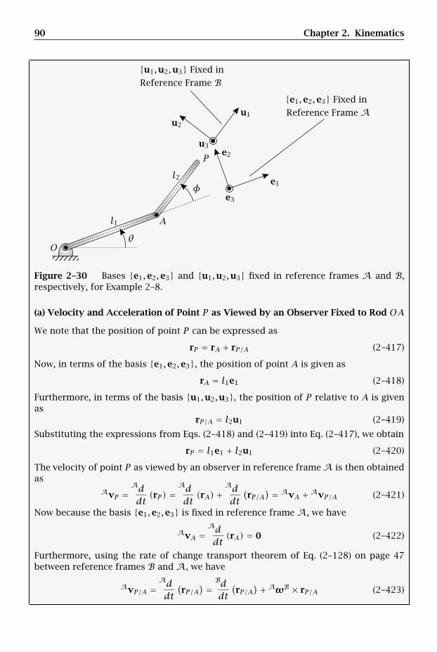
90 Chapter 2. Kinematics
e1
e2
e3
u1u2
u3
u1,u2,u3 Fixed in
e1,e2,e3 Fixed in
Reference Frame A
Reference Frame B
l1
l2
A
O
P
θ
φ
Figure 2–30 Bases e1,e2,e3 and u1,u2,u3 fixed in reference frames A and B,respectively, for Example 2–8.
(a) Velocity and Acceleration of Point P as Viewed by an Observer Fixed to Rod OA
We note that the position of point P can be expressed as
rP = rA + rP/A (2–417)
Now, in terms of the basis e1,e2,e3, the position of point A is given as
rA = l1e1 (2–418)
Furthermore, in terms of the basis u1,u2,u3, the position of P relative to A is givenas
rP/A = l2u1 (2–419)
Substituting the expressions from Eqs. (2–418) and (2–419) into Eq. (2–417), we obtain
rP = l1e1 + l2u1 (2–420)
The velocity of point P as viewed by an observer in reference frameA is then obtainedas
AvP =Addt(rP ) =
Addt(rA)+
Addt
(rP/A
) = AvA +AvP/A (2–421)
Now because the basis e1,e2,e3 is fixed in reference frame A, we have
AvA =Addt(rA) = 0 (2–422)
Furthermore, using the rate of change transport theorem of Eq. (2–128) on page 47between reference frames B and A, we have
AvP/A =Addt
(rP/A
) = Bddt
(rP/A
)+AωB × rP/A (2–423)
2.13 Practical Approach to Computing Velocity and Acceleration 91
Then, because rP/A is fixed in reference frame B, we have
Bddt
(rP/A
) = 0 (2–424)
Furthermore, because reference frame B is fixed in rod AP and the angleφ is measuredrelative to rod OA, we have AωB as
AωB = φu3 (2–425)
Consequently,AωB × rP/A = φu3 × l2u1 = l2φu2 (2–426)
Adding Eqs. (2–424) and (2–426), we obtain We then obtain AvP as
AvP = l2φu2 (2–427)
The acceleration of point P as viewed by an observer in reference frame A, denotedAaP , is obtained from Eq. (2–128) on page 47 as
AaP =Addt
(AvP
)=Bddt
(AvP
)+AωB × AvP (2–428)
Using the expression for AvP from Eq. (2–427), we see that
Bddt
(AvP
)= l2φu2 (2–429)
Furthermore, using AωB from Eq. (2–425), we obtain
AωB × AvP = φu3 × l2φu2 = −l2φ2u1 (2–430)
Consequently, we obtain AaP as
AaP = −l2φ2u1 + l2φu2 (2–431)
(b) Velocity and Acceleration of Point P as Viewed by an Observer Fixed to Ground
Using the expression for rP from Eq. (2–417), the velocity of point P as viewed by anobserver fixed to the ground is given as
FvP =Fddt(rP ) =
Fddt(rA)+
Fddt
(rP/A
) = FvA + FvP/A (2–432)
Observing from Eq. (2–418) that rA is expressed in the basis e1,e2,e3 and e1,e2,e3is fixed in reference frame A, the first term in Eq. (2–432) is obtained by applying therate of change transport theorem of Eq. (2–128) on page 47 between reference framesA and F as
FvA =Addt(rA)+ FωA × rA (2–433)
Because reference frame A is fixed to rod OA and rod OA rotates with angular rate θrelative to the ground, FωA is given as
FωA = θe3 (2–434)
92 Chapter 2. Kinematics
Furthermore, we have
Addt(rA) = 0 (2–435)
FωA × rA = θe3 × l1e1 = l1θe2 (2–436)
Adding Eqs. (2–435) and (2–436) gives
FvA = l1θe2 (2–437)
Next, observing from Eq. (2–419) that rP/A is expressed in terms of the basis u1,u2,u3and u1,u2,u3 is fixed in reference frame B, the second term in Eq. (2–432) is obtainedby applying the rate of change transport theorem of Eq. (2–128) on page 47 betweenreference frames B and F as
FvP/A =Bddt(rA)+ FωB × rP/A (2–438)
Now from the theorem of angular velocity addition as given in Eq. (2–136) on page 48,we have
FωB = FωA +AωB (2–439)
Using the expressions for AωB and FωA from Eqs. (2–425) and (2–434), respectively,and noting that e3 = u3, we obtain FωB as
FωB = θe3 + φu3 = (θ + φ)u3 (2–440)
Now we have
Bddt(rA) = 0 (2–441)
FωB × rP/A = (θ + φ)u3 × l2u1 = l2(θ + φ)u2 (2–442)
Adding Eqs. (2–441) and (2–442), we obtain FvP/A as
FvP/A = l2(θ + φ)u2 (2–443)
Then, adding Eqs. (2–437) and (2–443), we obtain FvP as
FvP = llθe2 + l2(θ + φ)u2 (2–444)
Using the expression for FvP from Eq. (2–444), the acceleration of point P as viewedby an observer in reference frame F is obtained as
FaP =Fddt
(FvP
)=Fddt
(FvA
)+Fddt
(FvP/A
)= FaA + FaP/A (2–445)
where
FvA = llθe2 (2–446)FvP/A = l2(θ + φ)u2 (2–447)

2.13 Practical Approach to Computing Velocity and Acceleration 93
Now since FvA is expressed in terms of the basis e1,e2,e3 and e1,e2,e3 is fixed inreference frame A, the first term in Eq. (2–445) is obtained using the rate of changetransport theorem of Eq. (2–128) on page 47 between reference frames A and F as
FaA =Fddt
(FvA
)=Addt
(FvA
)+ FωA × FvA (2–448)
Now we have
Addt
(FvA
)= llθe2 (2–449)
FωA × FvA = θe3 × llθe2 = −l1θ2e1 (2–450)
Adding Eqs. (2–449) and (2–450), we obtain
FaA = −l1θ2e1 + llθe2 (2–451)
Next, observing that FvP/A is expressed in terms of the basis u1,u2,u3 andu1,u2,u3 is fixed in reference frame B, the second term in Eq. (2–445) is obtainedby applying the rate of change transport theorem of Eq. (2–128) on page 47 betweenreference frames B and F as
FaP/A =Fddt
(FvP/A
)=Bddt
(FvP/A
)+ FωB × FvP/A (2–452)
Now we have
Bddt
(FvP/A
)= l2(θ + φ)u2 (2–453)
FωB × FvP/A = (θ + φ)u3 × l2(θ + φ)u2 = −l2(θ + φ)2u1 (2–454)
where in Eq. (2–454) we have used the expression for FωB from Eq. (2–440). AddingEqs. (2–453) and (2–454), we obtain
FaP/A = −l2(θ + φ)2u1 + l2(θ + φ)u2 (2–455)
Then, adding Eqs. (2–451) and (2–455), we obtain the acceleration of point P in refer-ence frame F as
FaP = −l1θ2e1 + l1θe2 − l2(θ + φ)2u1 + l2(θ + φ)u2 (2–456)
Example 2–9
A circular disk of radius r rotates about shaft OQ as shown in Fig. 2–31. Shaft OQ hasa length L, is oriented horizontally, and is rigidly attached to shaft BC , where shaft BCrotates with constant angular velocity Ω (where ‖Ω‖ = Ω) relative to the ground aboutthe vertical direction. Finally, point P is located on the edge of the disk. Knowing that
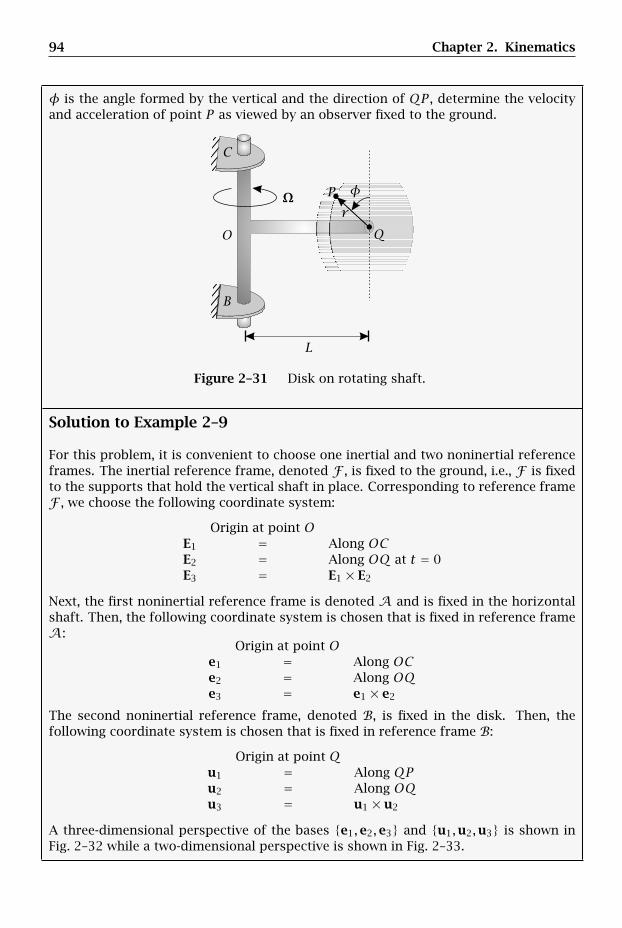
94 Chapter 2. Kinematics
φ is the angle formed by the vertical and the direction of QP , determine the velocityand acceleration of point P as viewed by an observer fixed to the ground.
r
B
C
L
O
P
Q
φΩ
Figure 2–31 Disk on rotating shaft.
Solution to Example 2–9
For this problem, it is convenient to choose one inertial and two noninertial referenceframes. The inertial reference frame, denoted F , is fixed to the ground, i.e., F is fixedto the supports that hold the vertical shaft in place. Corresponding to reference frameF , we choose the following coordinate system:
Origin at point OE1 = Along OCE2 = Along OQ at t = 0E3 = E1 × E2
Next, the first noninertial reference frame is denoted A and is fixed in the horizontalshaft. Then, the following coordinate system is chosen that is fixed in reference frameA:
Origin at point Oe1 = Along OCe2 = Along OQe3 = e1 × e2
The second noninertial reference frame, denoted B, is fixed in the disk. Then, thefollowing coordinate system is chosen that is fixed in reference frame B:
Origin at point Qu1 = Along QPu2 = Along OQu3 = u1 × u2
A three-dimensional perspective of the bases e1,e2,e3 and u1,u2,u3 is shown inFig. 2–32 while a two-dimensional perspective is shown in Fig. 2–33.
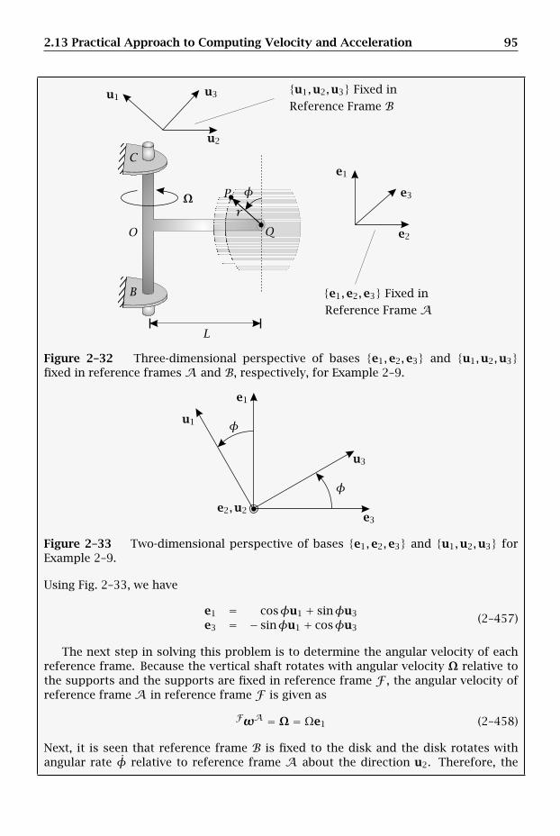
2.13 Practical Approach to Computing Velocity and Acceleration 95
u1,u2,u3 Fixed in
e1,e2,e3 Fixed in
Reference Frame A
Reference Frame B
e1
e2
e3
u1
u2
u3
r
B
C
L
O
P
Q
φΩ
Figure 2–32 Three-dimensional perspective of bases e1,e2,e3 and u1,u2,u3fixed in reference frames A and B, respectively, for Example 2–9.
e2,u2
e1
e3
u1
u3
φ
φ
Figure 2–33 Two-dimensional perspective of bases e1,e2,e3 and u1,u2,u3 forExample 2–9.
Using Fig. 2–33, we have
e1 = cosφu1 + sinφu3
e3 = − sinφu1 + cosφu3(2–457)
The next step in solving this problem is to determine the angular velocity of eachreference frame. Because the vertical shaft rotates with angular velocity Ω relative tothe supports and the supports are fixed in reference frame F , the angular velocity ofreference frame A in reference frame F is given as
FωA = Ω = Ωe1 (2–458)
Next, it is seen that reference frame B is fixed to the disk and the disk rotates withangular rate φ relative to reference frame A about the direction u2. Therefore, the
96 Chapter 2. Kinematics
angular velocity of reference frame B in reference frame A is given as
AωB = φu2 (2–459)
Then, using the theorem of addition of angular velocities as given in Eq. (2–136) onpage 48, the angular velocity of reference frame B in reference frame F is given as
FωB = FωA +AωB = Ωe1 + φu2 (2–460)
Now, in terms of the bases e1,e2,e3 and u1,u2,u3, the position of point P isgiven as
rP = rQ + rP/Q = Le2 + ru1 (2–461)
The velocity of point P in reference frame F is then obtained as
FvP =Fddt(rP ) =
Fddt
(rQ + rP/Q
)
=Fddt
(rQ)+ Fd
dt(rP/Q
) = FvQ + FvP/Q
(2–462)
where
rQ = Le2 (2–463)
rP/Q = ru1 (2–464)
Now, because rQ is expressed in the basis e1,e2,e3 and e1,e2,e3 is fixed in ref-erence frame A, the first term in Eq. (2–462) can be computed using the transporttheorem between reference frames A and F as
FvQ =Fddt
(rQ) = Ad
dt(rQ)+ FωA × rQ (2–465)
Then, because e1,e2,e3 is fixed in reference frameA and L is constant, the first termin Eq. (2–465) is zero, i.e.,
Addt
(rQ) = Ad
dt(Le2) = 0 (2–466)
Furthermore, using FωA from Eq. (2–458), the second term in Eq. (2–465) is obtainedas
FωA × rQ = Ωe1 × (Le2) = LΩe3 (2–467)
Adding the results of Eqs. (2–466) and (2–467), we obtain the velocity of point Q inreference frame F as
FvQ = LΩe3 (2–468)
Next, because rP/Q is expressed in the basis u1,u2,u3 and u1,u2,u3 is fixed inreference frame B, the second term in Eq. (2–462) is obtained using the rate of changetransport theorem of Eq. (2–128) on page 47 between reference frames B and F as
FvP/Q =Fddt
(rP/Q
) = Bddt
(rP/Q
)+ FωB × rP/Q (2–469)
2.13 Practical Approach to Computing Velocity and Acceleration 97
Because u1,u2,u3 is fixed in reference frame B and r is constant, the first term inEq. (2–469) is zero, i.e.,
Bddt
(rP/Q
) = Bddt(ru1) = 0 (2–470)
Furthermore, using FωB from Eq. (2–460), the second term in Eq. (2–469) is obtainedas
FωB × rP/Q =(Ωe1 + φu2
)× (ru1)
= rΩe1 × u1 + rφu2 × u1
= rΩe1 × u1 − rφu3
(2–471)
Then, using Eq. (2–457), we have
e1 × u1 = (cosφu1 + sinφu3)× u1 = sinφu2 (2–472)
Substituting the result of Eq. (2–472) into (2–471), we obtain
FωB × rP/Q = rΩ sinφu2 − rφu3 (2–473)
Adding the results of Eqs. (2–470) and (2–473), we obtain the velocity of point P relativeto point Q in reference frame F as
FvP/Q =Fddt
(rP/Q
) = rΩ sinφu2 − rφu3 (2–474)
Finally, adding the results of Eqs. (2–468) and (2–474), we obtain the velocity of pointP in reference frame F as
FvP = LΩe3 + rΩ sinφu2 − rφu3 (2–475)
It is noted that FvP can be expressed completely in terms of the basis e1,e2,e3 oru1,u2,u3 by applying the relationship of Eq. (2–457).
Now, the acceleration of point P in reference frame F is given as
FaP =Fddt
(FvP
)=Fddt
(FvQ + FvP/Q
)
=Fddt
(FvQ
)+Fddt
(FvP/Q
)= FaQ + FaP/Q
(2–476)
Restating Eqs. (2–468) and (2–474), the quantities FvQ and FvP/Q are given as
FvQ = LΩe3 (2–477)FvP/Q = rΩ sinφu2 − rφu3 (2–478)
Once again, because FvQ in Eq. (2–477) is expressed in the basis e1,e2,e3 ande1,e2,e3 is fixed in reference frame A, the first term in Eq. (2–476) can be obtainedby applying the transport theorem between reference frames A and F as
FaQ =Fddt
(FvQ
)=Addt
(FvQ
)+ FωA × FvQ (2–479)
98 Chapter 2. Kinematics
Now, because L and Ω are constant, we have from Eq. (2–477) that
Addt
(FvQ
)=Addt(LΩe3) = 0 (2–480)
Next, using the expression for FωA from Eq. (2–458), the second term in Eq. (2–479) isobtained as
FωA × FvQ = Ωe1 × LΩe3 = −LΩ2e2 (2–481)
Adding the results of Eqs. (2–480) and (2–481), we obtain the acceleration of point Qin reference frame F as
FaQ = −LΩ2e2 (2–482)
Then, because FvP/Q in Eq. (2–478) is expressed in the basis u1,u2,u3 and u1,u2,u3is fixed in reference frame B, the second term in Eq. (2–476) can be obtained by apply-ing the rate of change transport theorem between reference frames B and F as
FaP/Q =Fddt
(FvP/Q
)=Bddt
(FvP/Q
)+ FωB ×
(FvP/Q
)(2–483)
Using the expression for FvP/Q from Eq. (2–478), the first term in Eq. (2–483) becomes
Bddt
(FvP/Q
)= rΩφ cosφu2 − rφu3 (2–484)
Next, using FωB from Eq. (2–460), the second term in Eq. (2–483) is obtained as
FωB ×(FvP/Q
)= (Ωe1 + φu2)×
(rΩ sinφu2 − rφu3
)= rΩ2 sinφe1 × u2 − rΩφe1 × u3 − rφ2u1
(2–485)
Applying Eq. (2–457), we have
e1 × u2 = (cosφu1 + sinφu3)× u2 = cosφu3 − sinφu1 (2–486)
e1 × u3 = (cosφu1 + sinφu3)× u3 = − cosφu2 (2–487)
Substituting the results of Eqs. (2–486) and (2–487) into Eq. (2–485), we obtain
FωB ×(FvP/Q
)= rΩ2 sinφ(cosφu3 − sinφu1)+ rΩφ cosφu2 − rφ2u1
= rΩ2 cosφ sinφu3 − rΩ2 sin2φu1
+ rΩφ cosφu2 − rφ2u1
(2–488)
Then, adding the results of Eqs. (2–484) and (2–488), the acceleration of point P relativeto point Q in reference frame F is obtained as
FaP/Q = rΩφ cosφu2 − rφu3 + rΩ2 cosφ sinφu3
− rΩ2 sin2φu1 + rΩφ cosφu2 − rφ2u1(2–489)
Finally, adding the results of Eqs. (2–482) and (2–489), we obtain FaP as
FaP = −LΩ2e2 + rΩφ cosφu2 − rφu3 + rΩ2 cosφ sinφu3
− rΩ2 sin2φu1 + rΩφ cosφu2 − rφ2u1(2–490)
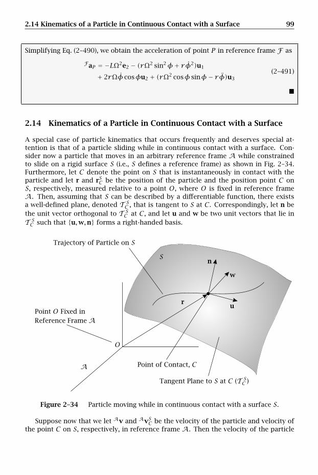
2.14 Kinematics of a Particle in Continuous Contact with a Surface 99
Simplifying Eq. (2–490), we obtain the acceleration of point P in reference frame F as
FaP = −LΩ2e2 − (rΩ2 sin2φ+ rφ2)u1
+ 2rΩφ cosφu2 + (rΩ2 cosφ sinφ− rφ)u3(2–491)
2.14 Kinematics of a Particle in Continuous Contact with a Surface
A special case of particle kinematics that occurs frequently and deserves special at-tention is that of a particle sliding while in continuous contact with a surface. Con-sider now a particle that moves in an arbitrary reference frame A while constrainedto slide on a rigid surface S (i.e., S defines a reference frame) as shown in Fig. 2–34.Furthermore, let C denote the point on S that is instantaneously in contact with theparticle and let r and rSC be the position of the particle and the position point C onS, respectively, measured relative to a point O, where O is fixed in reference frameA. Then, assuming that S can be described by a differentiable function, there existsa well-defined plane, denoted T S
C , that is tangent to S at C . Correspondingly, let n bethe unit vector orthogonal to T S
C at C , and let u and w be two unit vectors that lie inT SC such that u,w,n forms a right-handed basis.
Trajectory of Particle on S
Tangent Plane to S at C (T SC )
Point O Fixed in
A
Reference Frame A
Point of Contact, C
n
ru
w
O
S
Figure 2–34 Particle moving while in continuous contact with a surface S.
Suppose now that we let Av and AvSC be the velocity of the particle and velocity ofthe point C on S, respectively, in reference frame A. Then the velocity of the particle
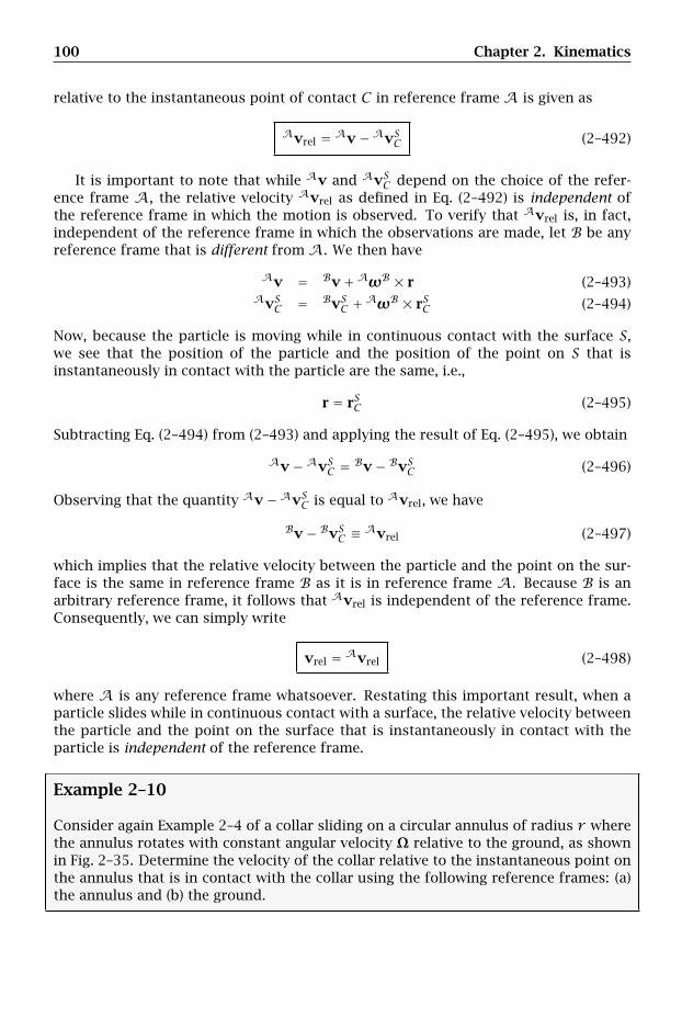
100 Chapter 2. Kinematics
relative to the instantaneous point of contact C in reference frame A is given as
Avrel = Av−AvSC (2–492)
It is important to note that while Av and AvSC depend on the choice of the refer-ence frame A, the relative velocity Avrel as defined in Eq. (2–492) is independent ofthe reference frame in which the motion is observed. To verify that Avrel is, in fact,independent of the reference frame in which the observations are made, let B be anyreference frame that is different from A. We then have
Av = Bv+AωB × r (2–493)AvSC = BvSC +AωB × rSC (2–494)
Now, because the particle is moving while in continuous contact with the surface S,we see that the position of the particle and the position of the point on S that isinstantaneously in contact with the particle are the same, i.e.,
r = rSC (2–495)
Subtracting Eq. (2–494) from (2–493) and applying the result of Eq. (2–495), we obtain
Av−AvSC = Bv− BvSC (2–496)
Observing that the quantity Av−AvSC is equal to Avrel, we have
Bv− BvSC ≡ Avrel (2–497)
which implies that the relative velocity between the particle and the point on the sur-face is the same in reference frame B as it is in reference frame A. Because B is anarbitrary reference frame, it follows that Avrel is independent of the reference frame.Consequently, we can simply write
vrel = Avrel (2–498)
where A is any reference frame whatsoever. Restating this important result, when aparticle slides while in continuous contact with a surface, the relative velocity betweenthe particle and the point on the surface that is instantaneously in contact with theparticle is independent of the reference frame.
Example 2–10
Consider again Example 2–4 of a collar sliding on a circular annulus of radius r wherethe annulus rotates with constant angular velocity Ω relative to the ground, as shownin Fig. 2–35. Determine the velocity of the collar relative to the instantaneous point onthe annulus that is in contact with the collar using the following reference frames: (a)the annulus and (b) the ground.
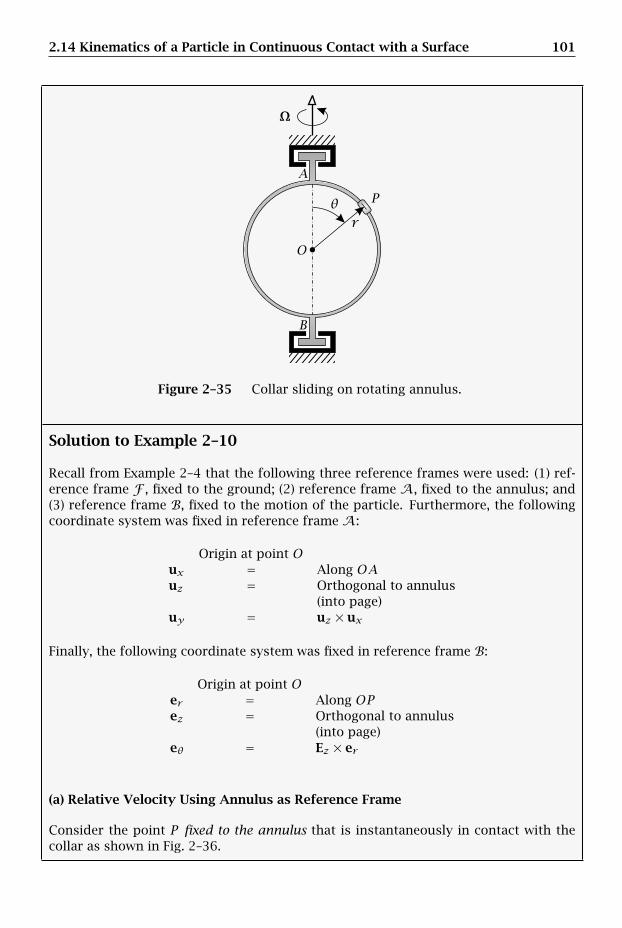
2.14 Kinematics of a Particle in Continuous Contact with a Surface 101
r
A
B
O
Pθ
Ω
Figure 2–35 Collar sliding on rotating annulus.
Solution to Example 2–10
Recall from Example 2–4 that the following three reference frames were used: (1) ref-erence frame F , fixed to the ground; (2) reference frame A, fixed to the annulus; and(3) reference frame B, fixed to the motion of the particle. Furthermore, the followingcoordinate system was fixed in reference frame A:
Origin at point Oux = Along OAuz = Orthogonal to annulus
(into page)uy = uz × ux
Finally, the following coordinate system was fixed in reference frame B:
Origin at point Oer = Along OPez = Orthogonal to annulus
(into page)eθ = Ez × er
(a) Relative Velocity Using Annulus as Reference Frame
Consider the point P fixed to the annulus that is instantaneously in contact with thecollar as shown in Fig. 2–36.
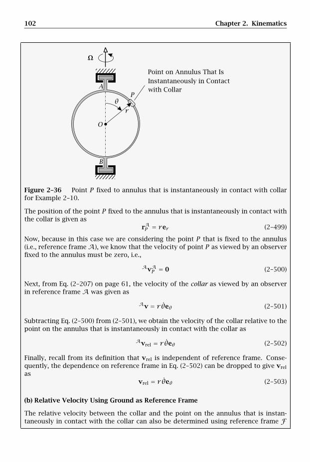
102 Chapter 2. Kinematics
Point on Annulus That IsInstantaneously in Contactwith Collar
r
A
B
O
Pθ
Ω
Figure 2–36 Point P fixed to annulus that is instantaneously in contact with collarfor Example 2–10.
The position of the point P fixed to the annulus that is instantaneously in contact withthe collar is given as
rAP = rer (2–499)
Now, because in this case we are considering the point P that is fixed to the annulus(i.e., reference frameA), we know that the velocity of point P as viewed by an observerfixed to the annulus must be zero, i.e.,
AvAP = 0 (2–500)
Next, from Eq. (2–207) on page 61, the velocity of the collar as viewed by an observerin reference frame A was given as
Av = r θeθ (2–501)
Subtracting Eq. (2–500) from (2–501), we obtain the velocity of the collar relative to thepoint on the annulus that is instantaneously in contact with the collar as
Avrel = r θeθ (2–502)
Finally, recall from its definition that vrel is independent of reference frame. Conse-quently, the dependence on reference frame in Eq. (2–502) can be dropped to give vrel
asvrel = r θeθ (2–503)
(b) Relative Velocity Using Ground as Reference Frame
The relative velocity between the collar and the point on the annulus that is instan-taneously in contact with the collar can also be determined using reference frame F
2.14 Kinematics of a Particle in Continuous Contact with a Surface 103
instead of reference frame A. First, the velocity of the point P that is fixed to thecollar and is instantaneously in contact with the annulus, as viewed by an observer inreference frame F , is given as
FvAP =F ddt
(rAP)=Addt
(rAP)+ FωA × rAP (2–504)
It is emphasized in Eq. (2–504) that, because we are considering the point P as fixedto the annulus (i.e., reference frame A), the velocity of point P in reference frame F iscomputed using the rate of change transport theorem between reference frame A andreference frame F . Then, because r is constant and er is now a direction that is fixedin reference frame A (because P is fixed in reference frame A), we have
Addt
(rAP)= 0 (2–505)
Next, using the expression for FωA from Eq. (2–213) on page 62, we have
FωA × rAP = Ωux × rer (2–506)
Then, substituting the expression for ux from Eq. (2–200) on page 61 into Eq. (2–506),we obtain
FωA × rAP = Ω(cosθer − sinθeθ)× rer = rΩ sinθez (2–507)
Adding Eqs. (2–507) and (2–505) gives
FvAP = rΩ sinθez (2–508)
Next, we have the velocity of the collar in reference frame F from Eq. (2–216) on page62 as
Fv = r θeθ + rΩ sinθez (2–509)
Subtracting Eq. (2–508) from (2–509), we obtain the velocity of the collar relative to thepoint on the annulus that is instantaneously in contact with the collar as
Fvrel = r θeθ + rΩ sinθez − rΩ sinθez = r θeθ (2–510)
It is seen that the result of Eq. (2–510) is identical to that of Eq. (2–503), i.e., the quantityvrel is the same regardless of whether the relative velocity is computed in referenceframe A or reference frame F . Eliminating the dependence in Eq. (2–510) on thereference frame, we obtain vrel as
vrel = r θeθ (2–511)
104 Chapter 2. Kinematics
2.15 Kinematics of Rigid Bodies
A rigid body, denoted R, is a collection of points, each of which may or may not havemass, such that the distance between any two points on the body is a constant. Giventhis definition, it is seen that a rigid body is kinematically identical to a reference frame(the only difference being that a reference frame consists of a collection of points inspace and the points are massless). Thus, from the standpoint of kinematics, a rigidbody and a reference frame are interchangeable, i.e., kinematically, a rigid body is areference frame. Now, because a rigid body R defines a reference frame, it followsdirectly that the angular velocity of a rigid body R as viewed by an observer in anarbitrary reference frame A is the same as the angular velocity of the reference framedefined by the rigid body. Consequently, when referring to the angular velocity ofa rigid body, the notation AωR will mean the angular velocity of the rigid body R(i.e., the angular velocity of reference frame R) as viewed by an observer in referenceframe A. Finally, any collection of points that are not part of the rigid body but arefixed to the reference frame defined by the rigid body is called an extension of the rigidbody.
2.15.1 Configuration and Degrees of Freedom of a Rigid Body
In Section 2.4 we discussed the three scalar quantities that are required to describethe configuration (i.e., the position) of a point moving in R3 without any constraints.Consequently, a point (i.e., a particle) moving in R3 without any constraints has threedegrees of freedom. However, in order to specify the configuration of a rigid body,more quantities are required than are required to specify the configuration of a point.In other words, the number of degrees of freedom for a rigid body is greater than thenumber of degrees of freedom of a point. We now discuss the configuration of a rigidbody moving without constraints in R3.
Using the schematic of the configuration of a rigid body R as given in Fig. 2–37, wecan determine the number of degrees of freedom of an unconstrained rigid body asfollows. First, as already discussed, three quantities are required to describe the con-figuration of an arbitrary point Q fixed in the rigid body R. In addition, we know thata rigid body defines a reference frame and that the rate of change of the orientation ofthe rigid body R in an arbitrary reference frame A is obtained from the angular veloc-ity of R in reference frame A, AωR. Furthermore, we know that the angular velocityof a rigid body is specified by three scalar quantities. Consequently, it must be thecase that the orientation of a rigid body can be described using three scalar quantities.Combining the three quantities required to describe the configuration of an arbitrarypoint on the body with the three quantities required to describe the orientation of theentire body relative to an arbitrary reference frame A, we see that a total of six scalarquantities are required to specify completely the configuration of an unconstrainedrigid body R. An unconstrained rigid body is thus said to have six degrees of freedom.
2.15.2 Rigid Body Motion Using Body-Fixed Coordinate Systems
While in principle the motion of a rigid body can be described using a coordinatesystem fixed in any reference frame whatsoever, in practice it is inconvenient to choosethe coordinate system in such an arbitrary manner. Instead, it is useful to use the
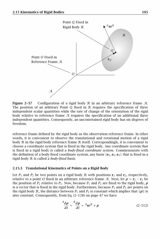
2.15 Kinematics of Rigid Bodies 105
Point O Fixed in
Point Q Fixed in
A
R
Reference Frame A
Rigid Body R AωR
rQ
O
Q
Figure 2–37 Configuration of a rigid body R in an arbitrary reference frame A.The position of an arbitrary Point Q fixed in R requires the specification of threeindependent scalar quantities while the rate of change of the orientation of the rigidbody relative to reference frame A requires the specification of an additional threeindependent quantities. Consequently, an unconstrained rigid body has six degrees offreedom.
reference frame defined by the rigid body as the observation reference frame. In otherwords, it is convenient to observe the translational and rotational motion of a rigidbody R in the rigid body reference frame R itself. Correspondingly, it is convenient tochoose a coordinate system that is fixed in the rigid body. Any coordinate system thatis fixed in a rigid body is called a body-fixed coordinate system. Commensurate withthe definition of a body-fixed coordinate system, any basis e1,e2,e3 that is fixed in arigid body R is called a body-fixed basis.
2.15.3 Translational Kinematics of Points on a Rigid Body
Let P1 and P2 be two points on a rigid body R with positions r1 and r2, respectively,relative to a point O fixed in an arbitrary reference frame A. Next, let ρ = r2 − r1 bethe position of P2 relative to P1. Now, because P1 and P2 are fixed to the rigid body, ρis a vector that is fixed in the rigid body. Furthermore, because P1 and P2 are points onthe rigid body R, the distance between P1 and P2 is constant which implies that ‖ρ‖ isalso constant. Consequently, from Eq. (2–128) on page 47 we have
Adρdt
=Rdρdt
+AωR × ρ (2–512)

106 Chapter 2. Kinematics
However, because ρ is fixed in R, the rate of change of ρ as viewed by an observerfixed to R is zero, i.e.,
Rdρdt
= 0 (2–513)
Consequently, we haveAdρdt
= AωR × ρ (2–514)
It is seen that Eq. (2–513) is valid for any two points that are fixed in a rigid body.Furthermore, we have
Adρdt
=Addt(r2 − r1) = Av2 −Av1 (2–515)
Using the result of Eq. (2–514), we obtain
Av2 −Av1 = AωR × (r2 − r1) (2–516)
Equation (2–516) can be rewritten as
Av2 = Av1 +AωR × (r2 − r1) (2–517)
Equation (2–517) relates the velocity between any two points on a rigid body as viewedby an observer in reference frame A.
The acceleration between any two points on a rigid body as viewed by an observerin reference frame A is obtained by applying Eq. (2–128) on page 47 to Eq. (2–517). Wethen have
Addt
(Av2
)=Addt
(Av1
)+Addt
(AωR × (r2 − r1)
)(2–518)
Now we note thatAddt
(Av1
)= Aa1
Addt
(Av2
)= Aa2
(2–519)
Consequently, Eq. (2–518) can be rewritten as
Aa2 = Aa1 +Addt
(AωR × (r2 − r1)
)(2–520)
The second term in Eq. (2–520) can be written as
Addt
(AωR × (r2 − r1)
)=Addt
(AωR
)× (r2 − r1)+AωR ×
Addt(r2 − r1) (2–521)
Now we recall thatAddt
(AωR
)= AαR (2–522)
where AαR is the angular acceleration of R as viewed by an observer in referenceframe A. Also, using Eq. (2–516), we have
Addt
(AωR × (r2 − r1)
)= AαR × (r2 − r1)+AωR ×
[AωR × (r2 − r1)
](2–523)
2.15 Kinematics of Rigid Bodies 107
Equation (2–520) then simplifies to
Aa2 = Aa1 +AαR × (r2 − r1)+AωR ×[AωR × (r2 − r1)
](2–524)
Equation (2–524) relates the acceleration between any two points on a rigid body asviewed by an observer in reference frame A.
2.15.4 Kinematics of Rolling and Sliding Rigid Bodies
Many applications of rigid body motion involve two rigid bodies moving while main-taining contact with one another. The two important forms of contact between rigidbodies are rolling and sliding. We now discuss the kinematics associated with two rigidbodies moving while either rolling or sliding relative to one another.7
Rolling and Sliding Between Two Moving Rigid Bodies
Consider a rigid body R, called the primary rigid body, moving in an arbitrary ref-erence frame A while maintaining continuous contact over a nonzero time intervalt ∈ [t1, t2] with a rigid body S, called the secondary rigid body, as shown in Fig. 2–38.Furthermore, let O be a point fixed in reference frame A and let Q be a point fixed inthe reference frame defined by R.8 Finally, assume that the motion of S in referenceframe A is known (i.e., the velocity and acceleration of every point on S in referenceframe A is known).
Now, because R is in contact with S, at every instant of the contacting motionthere exists a point C , called the instantaneous point of contact, that is common toboth R and S. Moreover, because both bodies are moving, the instantaneous point ofcontact C changes continuously during the contacting motion. Next, assuming that thesurfaces of R and S can each be described by differentiable functions, there exists awell-defined plane of contact, denoted T R
C = T SC ≡ TC , that is tangent to both R and S
at the instantaneous point of contact C . Then, let n be the unit vector in the directionorthogonal to TC .
Suppose now that we let AvRC and AvSC be the velocity of point C on the rigid bodyR and the velocity of point C on the rigid body S, respectively, in reference frame A.9
Then, the rigid body R is said to instantaneously roll or roll without slip on S if thevelocity of point C on R as viewed by an observer in reference frame A is equal tothe velocity of point C on S as viewed by an observer in reference frame A, i.e., thecondition for R to roll on S is given as
AvRC = AvSC (2–525)
7The approach used in this section is inspired by the description of rolling and sliding as given inO’Reilly (2001), the key difference being that in the description given in O’Reilly (2001) the secondary rigidbody is a fixed surface whereas in the description given here the secondary rigid body may be moving.The inclusion of a moving secondary rigid body is important because such situations are encounteredin practice (e.g., Problem 2.14 on page 136 is an example of a system of two rigid bodies that are bothmoving while maintaining continuous contact with one another).
8While point Q in Fig. 2–38 is depicted as being a point on the rigid body R, in general the point Q maybe a point either on or off the rigid body. In the case that point Q lies off R, we assume in this analysisthat Q lies in an extension of R and thus is fixed in R.
9It is emphasized that when using the notation AvRC we are considering point C to be a point that isfixed in the rigid body R.
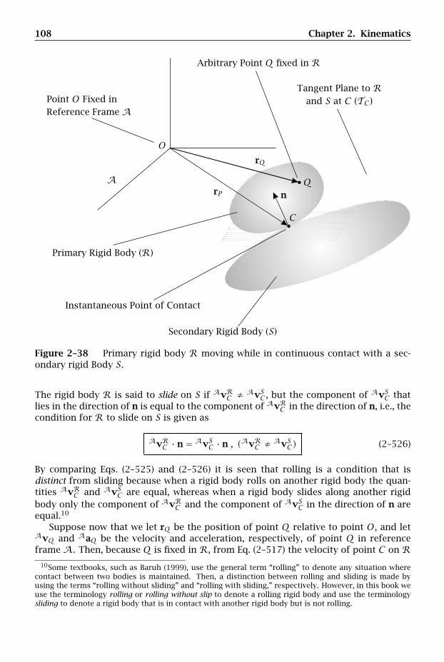
108 Chapter 2. Kinematics
Primary Rigid Body (R)
Secondary Rigid Body (S)
Tangent Plane to Rand S at C (TC )
Arbitrary Point Q fixed in R
Instantaneous Point of Contact
Point O Fixed in
A
Reference Frame A
nrP
rQ
C
O
Q
Figure 2–38 Primary rigid body R moving while in continuous contact with a sec-ondary rigid Body S.
The rigid body R is said to slide on S if AvRC ≠AvSC , but the component of AvSC that
lies in the direction of n is equal to the component of AvRC in the direction of n, i.e., thecondition for R to slide on S is given as
AvRC · n = AvSC · n , (AvRC ≠AvSC) (2–526)
By comparing Eqs. (2–525) and (2–526) it is seen that rolling is a condition that isdistinct from sliding because when a rigid body rolls on another rigid body the quan-tities AvRC and AvSC are equal, whereas when a rigid body slides along another rigidbody only the component of AvRC and the component of AvSC in the direction of n areequal.10
Suppose now that we let rQ be the position of point Q relative to point O, and letAvQ and AaQ be the velocity and acceleration, respectively, of point Q in referenceframe A. Then, because Q is fixed in R, from Eq. (2–517) the velocity of point C on R
10Some textbooks, such as Baruh (1999), use the general term “rolling” to denote any situation wherecontact between two bodies is maintained. Then, a distinction between rolling and sliding is made byusing the terms “rolling without sliding” and “rolling with sliding,” respectively. However, in this book weuse the terminology rolling or rolling without slip to denote a rolling rigid body and use the terminologysliding to denote a rigid body that is in contact with another rigid body but is not rolling.
2.15 Kinematics of Rigid Bodies 109
in reference frame A is given as
AvRC = AvQ +AωR × (rC − rQ) (2–527)
Substituting AvRC from Eq. (2–527) into (2–525), we have
AvQ +AωR × (rC − rQ) = AvSC (2–528)
Equation (2–528) provides an alternate expression for the case where the rigid body Rrolls on the rigid body S. Similarly, substituting AvRC from Eq. (2–527) into (2–526), wehave [
AvQ +AωR × (rC − rQ)]· n = AvSC · n (2–529)
Equation (2–529) provides an alternate expression for the case where the rigid body Rslides on the rigid body S.
Rolling and Sliding of a Rigid Body Along a Fixed Surface
An important special case of rolling and sliding that occurs frequently is that of arigid body rolling or sliding on an absolutely fixed body. Furthermore, suppose thatobservations of the motion are made in a fixed inertial reference frame F . Then,because S is absolutely fixed, S itself is a fixed inertial reference frame (i.e., S ≡ F ).Therefore, the velocity of the instantaneous point of contact in reference frame F iszero, i.e.,
FvSC = 0 (2–530)
Consequently, the rolling condition of Eq. (2–525) simplifies to (O’Reilly, 2001)
FvRC = FvSC = 0 (2–531)
Furthermore, the sliding condition of Eq. (2–526) simplifies to (O’Reilly, 2001)
FvRC · n = 0 (2–532)
In other words, when a rigid body rolls on a fixed rigid body, the velocity of the in-stantaneous point of contact C on R is zero when viewed by an observer in the fixedinertial reference frame F . Now, it is important to realize that, while FvRC may be zero,the acceleration of C on R in F , FaRC , is not zero. The fact that FaRC is not zero is seenby applying Eq. (2–524) as
AaRC = AaQ +AαR × (rC − rQ)+AωR ×[AωR × (rC − rQ)
](2–533)
Equation (2–533) shows that, in general, the acceleration of the point of contact, AaRC ,is not zero for the case of a rigid body rolling on an absolutely fixed surface. Lastly,it is noted that Eqs. (2–531) and (2–532) are valid only when the rigid body S definesa fixed inertial reference frame; in the general case of a rigid body in contact with amoving rigid body, either Eq. (2–525) or (2–526) must be applied.
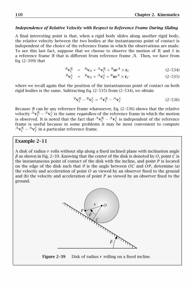
110 Chapter 2. Kinematics
Independence of Relative Velocity with Respect to Reference Frame During Sliding
A final interesting point is that, when a rigid body slides along another rigid body,the relative velocity between the two bodies at the instantaneous point of contact isindependent of the choice of the reference frame in which the observations are made.To see this last fact, suppose that we choose to observe the motion of R and S ina reference frame B that is different from reference frame A. Then, we have fromEq. (2–399) that
BvRC = BvO +AvRC + BωA × rC (2–534)BvSC = BvO +AvSC + BωA × rC (2–535)
where we recall again that the position of the instantaneous point of contact on bothrigid bodies is the same. Subtracting Eq. (2–535) from (2–534), we obtain
BvRC − BvSC = AvRC −AvSC (2–536)
Because B can be any reference frame whatsoever, Eq. (2–536) shows that the relativevelocity AvRC −AvSC is the same regardless of the reference frame in which the motionis observed. It is noted that the fact that AvRC − AvSC is independent of the referenceframe is useful because in some problems it may be most convenient to computeAvRC −AvSC in a particular reference frame.
Example 2–11
A disk of radius r rolls without slip along a fixed inclined plane with inclination angleβ as shown in Fig. 2–39. Knowing that the center of the disk is denoted by O, point C isthe instantaneous point of contact of the disk with the incline, and point P is locatedon the edge of the disk such that θ is the angle between OC and OP , determine (a)the velocity and acceleration of point O as viewed by an observer fixed to the groundand (b) the velocity and acceleration of point P as viewed by an observer fixed to theground.
r
C
OP
β
θ
Figure 2–39 Disk of radius r rolling on a fixed incline.
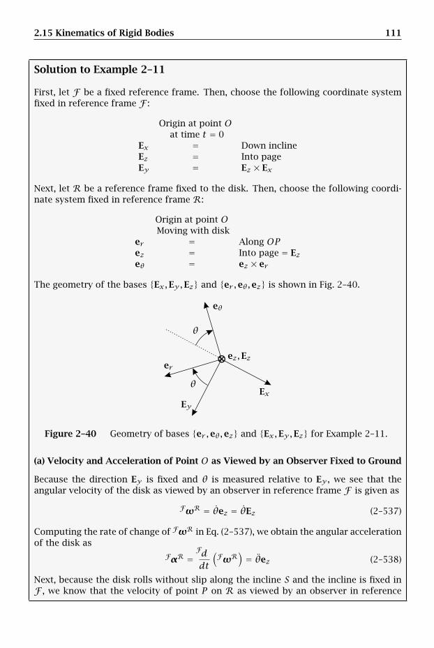
2.15 Kinematics of Rigid Bodies 111
Solution to Example 2–11
First, let F be a fixed reference frame. Then, choose the following coordinate systemfixed in reference frame F :
Origin at point Oat time t = 0
Ex = Down inclineEz = Into pageEy = Ez × Ex
Next, let R be a reference frame fixed to the disk. Then, choose the following coordi-nate system fixed in reference frame R:
Origin at point OMoving with disk
er = Along OPez = Into page = Ezeθ = ez × er
The geometry of the bases Ex,Ey,Ez and er ,eθ,ez is shown in Fig. 2–40.
⊗er
eθ
ExEy
ez,Ez
θ
θ
Figure 2–40 Geometry of bases er ,eθ,ez and Ex,Ey,Ez for Example 2–11.
(a) Velocity and Acceleration of Point O as Viewed by an Observer Fixed to Ground
Because the direction Ey is fixed and θ is measured relative to Ey , we see that theangular velocity of the disk as viewed by an observer in reference frame F is given as
FωR = θez = θEz (2–537)
Computing the rate of change of FωR in Eq. (2–537), we obtain the angular accelerationof the disk as
FαR =Fddt
(FωR
)= θez (2–538)
Next, because the disk rolls without slip along the incline S and the incline is fixed inF , we know that the velocity of point P on R as viewed by an observer in reference
112 Chapter 2. Kinematics
frame F is zero, i.e., FvC = 0. Then, using the result of Eq. (2–517) on page 106, wehave
FvO = FvC + FωR × (rO − rC) (2–539)
Now, in terms of the basis Ex,Ey,Ez, rO − rC is given as
rO − rC = −rEy (2–540)
Then, using the angular velocity from Eq. (2–537) and the fact that FvC = 0, Eq. (2–539)becomes
FvO = θEz × (−rEy) = r θEx (2–541)
The position of point O is then found by integrating Eq. (2–541) as
rO =∫ t
0r θdτ Ex =
∫ θ0rdνEx = rθEx (2–542)
where τ and ν are dummy variables of integration. Furthermore, using FvO fromEq. (2–541), we obtain the acceleration of point O as viewed by an observer in referenceframe F as
FaO = r θEx (2–543)
(b) Velocity and Acceleration of Point P as Viewed by an Observer Fixed to Ground
First, we haverP − rO = rer (2–544)
Then, from Eq. (2–517) on page 106, we have
FvP = FvO + FωR × (rP − rO) = FvO + θEz × rer = FvO + r θeθ (2–545)
Using FvO from Eq. (2–541), we obtain FvP as
FvP = r θEx + r θeθ (2–546)
Furthermore, from Eq. (2–524), we have
FaP = FaO + FαR × (rP − rO)+ FωR ×[FωR × (rP − rO)
](2–547)
Substituting FωR from Eq. (2–537), FαR from Eq. (2–538), and rP−rO from Eq. (2–544),we obtain
FaP = FaO + θEz × rer + θEz ×[θEz × rer
](2–548)
Simplifying Eq. (2–548) gives
FaP = FaO + r θeθ − r θ2er (2–549)
Using FaO from Eq. (2–543), we obtain the acceleration of point P as
FaP = r θEx + r θeθ − r θ2er (2–550)
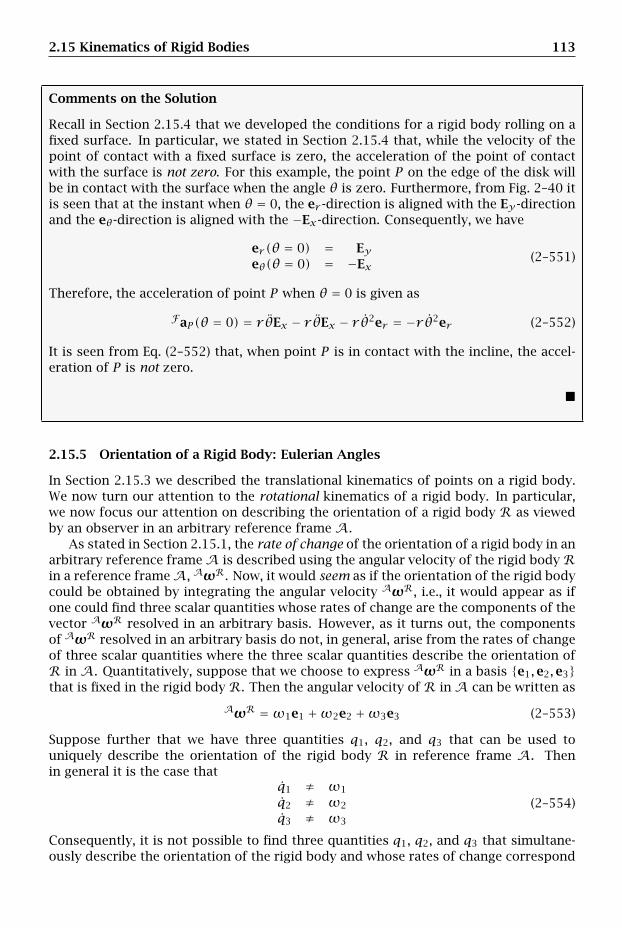
2.15 Kinematics of Rigid Bodies 113
Comments on the Solution
Recall in Section 2.15.4 that we developed the conditions for a rigid body rolling on afixed surface. In particular, we stated in Section 2.15.4 that, while the velocity of thepoint of contact with a fixed surface is zero, the acceleration of the point of contactwith the surface is not zero. For this example, the point P on the edge of the disk willbe in contact with the surface when the angle θ is zero. Furthermore, from Fig. 2–40 itis seen that at the instant when θ = 0, the er -direction is aligned with the Ey -directionand the eθ-direction is aligned with the −Ex-direction. Consequently, we have
er (θ = 0) = Eyeθ(θ = 0) = −Ex
(2–551)
Therefore, the acceleration of point P when θ = 0 is given as
FaP (θ = 0) = r θEx − r θEx − r θ2er = −r θ2er (2–552)
It is seen from Eq. (2–552) that, when point P is in contact with the incline, the accel-eration of P is not zero.
2.15.5 Orientation of a Rigid Body: Eulerian Angles
In Section 2.15.3 we described the translational kinematics of points on a rigid body.We now turn our attention to the rotational kinematics of a rigid body. In particular,we now focus our attention on describing the orientation of a rigid body R as viewedby an observer in an arbitrary reference frame A.
As stated in Section 2.15.1, the rate of change of the orientation of a rigid body in anarbitrary reference frameA is described using the angular velocity of the rigid bodyRin a reference frameA, AωR. Now, it would seem as if the orientation of the rigid bodycould be obtained by integrating the angular velocity AωR, i.e., it would appear as ifone could find three scalar quantities whose rates of change are the components of thevector AωR resolved in an arbitrary basis. However, as it turns out, the componentsof AωR resolved in an arbitrary basis do not, in general, arise from the rates of changeof three scalar quantities where the three scalar quantities describe the orientation ofR in A. Quantitatively, suppose that we choose to express AωR in a basis e1,e2,e3that is fixed in the rigid body R. Then the angular velocity of R in A can be written as
AωR =ω1e1 +ω2e2 +ω3e3 (2–553)
Suppose further that we have three quantities q1, q2, and q3 that can be used touniquely describe the orientation of the rigid body R in reference frame A. Thenin general it is the case that
q1 ≠ ω1
q2 ≠ ω2
q3 ≠ ω3
(2–554)
Consequently, it is not possible to find three quantities q1, q2, and q3 that simultane-ously describe the orientation of the rigid body and whose rates of change correspond
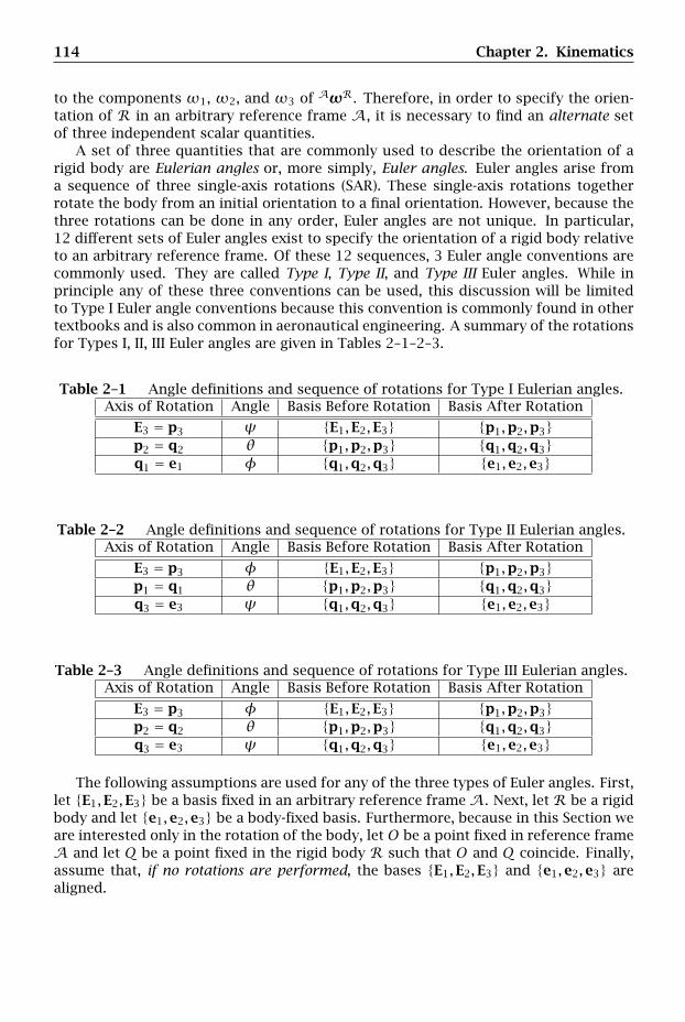
114 Chapter 2. Kinematics
to the components ω1, ω2, and ω3 of AωR. Therefore, in order to specify the orien-tation of R in an arbitrary reference frame A, it is necessary to find an alternate setof three independent scalar quantities.
A set of three quantities that are commonly used to describe the orientation of arigid body are Eulerian angles or, more simply, Euler angles. Euler angles arise froma sequence of three single-axis rotations (SAR). These single-axis rotations togetherrotate the body from an initial orientation to a final orientation. However, because thethree rotations can be done in any order, Euler angles are not unique. In particular,12 different sets of Euler angles exist to specify the orientation of a rigid body relativeto an arbitrary reference frame. Of these 12 sequences, 3 Euler angle conventions arecommonly used. They are called Type I, Type II, and Type III Euler angles. While inprinciple any of these three conventions can be used, this discussion will be limitedto Type I Euler angle conventions because this convention is commonly found in othertextbooks and is also common in aeronautical engineering. A summary of the rotationsfor Types I, II, III Euler angles are given in Tables 2–1–2–3.
Table 2–1 Angle definitions and sequence of rotations for Type I Eulerian angles.Axis of Rotation Angle Basis Before Rotation Basis After Rotation
E3 = p3 ψ E1,E2,E3 p1,p2,p3p2 = q2 θ p1,p2,p3 q1,q2,q3q1 = e1 φ q1,q2,q3 e1,e2,e3
Table 2–2 Angle definitions and sequence of rotations for Type II Eulerian angles.Axis of Rotation Angle Basis Before Rotation Basis After Rotation
E3 = p3 φ E1,E2,E3 p1,p2,p3p1 = q1 θ p1,p2,p3 q1,q2,q3q3 = e3 ψ q1,q2,q3 e1,e2,e3
Table 2–3 Angle definitions and sequence of rotations for Type III Eulerian angles.Axis of Rotation Angle Basis Before Rotation Basis After Rotation
E3 = p3 φ E1,E2,E3 p1,p2,p3p2 = q2 θ p1,p2,p3 q1,q2,q3q3 = e3 ψ q1,q2,q3 e1,e2,e3
The following assumptions are used for any of the three types of Euler angles. First,let E1,E2,E3 be a basis fixed in an arbitrary reference frame A. Next, let R be a rigidbody and let e1,e2,e3 be a body-fixed basis. Furthermore, because in this Section weare interested only in the rotation of the body, let O be a point fixed in reference frameA and let Q be a point fixed in the rigid body R such that O and Q coincide. Finally,assume that, if no rotations are performed, the bases E1,E2,E3 and e1,e2,e3 arealigned.
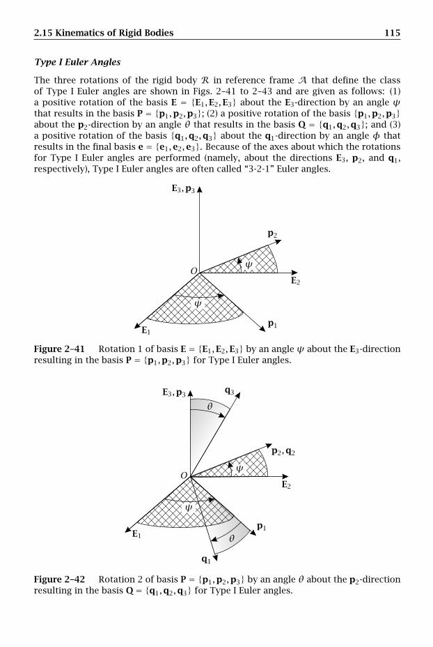
2.15 Kinematics of Rigid Bodies 115
Type I Euler Angles
The three rotations of the rigid body R in reference frame A that define the classof Type I Euler angles are shown in Figs. 2–41 to 2–43 and are given as follows: (1)a positive rotation of the basis E = E1,E2,E3 about the E3-direction by an angle ψthat results in the basis P = p1,p2,p3; (2) a positive rotation of the basis p1,p2,p3about the p2-direction by an angle θ that results in the basis Q = q1,q2,q3; and (3)a positive rotation of the basis q1,q2,q3 about the q1-direction by an angle φ thatresults in the final basis e = e1,e2,e3. Because of the axes about which the rotationsfor Type I Euler angles are performed (namely, about the directions E3, p2, and q1,respectively), Type I Euler angles are often called “3-2-1” Euler angles.
E3,p3
E1
E2
p1
p2
Oψ
ψ
Figure 2–41 Rotation 1 of basis E = E1,E2,E3 by an angle ψ about the E3-directionresulting in the basis P = p1,p2,p3 for Type I Euler angles.
E3,p3
p2,q2
E1
E2
p1
q1
q3
O
θ
θ
ψ
ψ
Figure 2–42 Rotation 2 of basis P = p1,p2,p3 by an angle θ about the p2-directionresulting in the basis Q = q1,q2,q3 for Type I Euler angles.
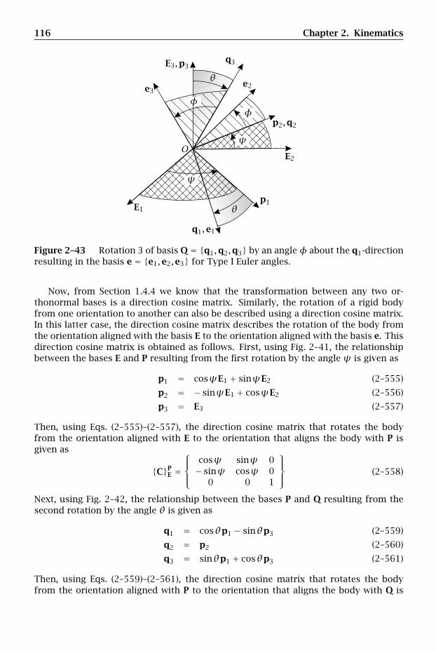
116 Chapter 2. Kinematics
E3,p3
p2,q2
q1,e1
e2e3
E1
E2
p1
q3
O
θ
θ
ψ
ψ
φφ
Figure 2–43 Rotation 3 of basis Q = q1,q2,q3 by an angleφ about the q1-directionresulting in the basis e = e1,e2,e3 for Type I Euler angles.
Now, from Section 1.4.4 we know that the transformation between any two or-thonormal bases is a direction cosine matrix. Similarly, the rotation of a rigid bodyfrom one orientation to another can also be described using a direction cosine matrix.In this latter case, the direction cosine matrix describes the rotation of the body fromthe orientation aligned with the basis E to the orientation aligned with the basis e. Thisdirection cosine matrix is obtained as follows. First, using Fig. 2–41, the relationshipbetween the bases E and P resulting from the first rotation by the angle ψ is given as
p1 = cosψE1 + sinψE2 (2–555)
p2 = − sinψE1 + cosψE2 (2–556)
p3 = E3 (2–557)
Then, using Eqs. (2–555)–(2–557), the direction cosine matrix that rotates the bodyfrom the orientation aligned with E to the orientation that aligns the body with P isgiven as
CPE =
⎧⎪⎨⎪⎩
cosψ sinψ 0− sinψ cosψ 0
0 0 1
⎫⎪⎬⎪⎭ (2–558)
Next, using Fig. 2–42, the relationship between the bases P and Q resulting from thesecond rotation by the angle θ is given as
q1 = cosθp1 − sinθp3 (2–559)
q2 = p2 (2–560)
q3 = sinθp1 + cosθp3 (2–561)
Then, using Eqs. (2–559)–(2–561), the direction cosine matrix that rotates the bodyfrom the orientation aligned with P to the orientation that aligns the body with Q is
2.15 Kinematics of Rigid Bodies 117
given as
CQP =
⎧⎪⎨⎪⎩
cosθ 0 − sinθ0 1 0
sinθ 0 cosθ
⎫⎪⎬⎪⎭ (2–562)
Finally, using Fig. 2–43, the relationship between the bases Q and e resulting from thethird rotation by φ is given as
e1 = q1 (2–563)
e2 = cosφq2 + sinφq3 (2–564)
e3 = − sinφq2 + cosφq3 (2–565)
Then, using Eqs. (2–563)–(2–565), the direction cosine matrix that rotates the bodyfrom the orientation aligned with Q to the orientation that aligns the body with e isgiven as
CeQ =
⎧⎪⎨⎪⎩
1 0 00 cosφ sinφ0 − sinφ cosφ
⎫⎪⎬⎪⎭ (2–566)
Using Eqs. (2–558), (2–562), and (2–566), the rotation of the body from the initial ori-entation aligned with the basis E to the final orientation aligned with the basis e isobtained by multiplying the three direction cosine matrices CP
E, CQP , and Ce
Q as
CeE = Ce
Q CQP CP
E (2–567)
Now, because the direction cosine matrices CPE, CQ
P , and CeQ correspond to rota-
tions by the angles ψ, θ, and φ, respectively, we can write
CPE = Cψ
CQP = Cθ
CeQ = Cφ
(2–568)
Using the expressions in Eq. (2–568), the direction cosine matrix that rotates the rigidbody from the initial orientation aligned with basis E to the final orientation alignedwith the basis e is given as
CeE = Cφ Cθ Cψ (2–569)
Finally, using the expressions for CPE, CQ
P , and CeQ from Eqs. (2–558), (2–562), and
(2–566), we obtain the direction cosine matrix from E to e as
CeE =
⎧⎪⎪⎪⎪⎪⎨⎪⎪⎪⎪⎪⎩
cosθ cosψ cosθ sinψ − sinθ(− cosφ sinψ (cosφ cosψ sinφ cosθ
+ sinφ sinθ cosψ) + sinφ sinθ sinψ)(sinφ sinψ (− sinφ cosψ cosφ cosθ
+ cosφ sinθ cosψ) + cosφ sinθ sinψ)
⎫⎪⎪⎪⎪⎪⎬⎪⎪⎪⎪⎪⎭
(2–570)
For completeness, it is noted that the direction cosine tensor that rotates the rigid body
118 Chapter 2. Kinematics
from the orientation aligned with the basis E to the basis aligned with e is given as
C = cosθ cosψe1 ⊗ E1 + cosθ sinψe1 ⊗ E2 − sinθe1 ⊗ E3
+ (− cosφ sinψ + sinφ sinθ cosψ)e2 ⊗ E1
+ (cosφ cosψ + sinφ sinθ sinψ)e2 ⊗ E2
+ sinφ cosθe2 ⊗ E3
+ (sinφ sinψ + cosφ sinθ cosψ)e3 ⊗ E1
+ (− sinφ cosψ + cosφ sinθ sinψ)e3 ⊗ E2
+ cosφ cosθe3 ⊗ E3
(2–571)
Now we can obtain an expression for the angular velocity of the rigid body R in thereference frame A (i.e., AωR) as follows. First, suppose that we let P denote the refer-ence frame in which the basis P is fixed. Then, because the first Euler angle rotation isperformed relative to the basis E1,E2,E3 and E1,E2,E3 is fixed in reference frameA, the angular velocity of reference frame P in reference frame A is given as
AωP = ψE3 = ψp3 (2–572)
Next, suppose that we let Q denote the reference frame in which the basis Q is fixed.Then, because the second Euler angle rotation is performed relative to the basis P andP is fixed in reference frame P, the angular velocity of reference frame Q in referenceframe P is given as
PωQ = θp2 = θq2 (2–573)
Finally, observing that the third rotation is performed relative to the basis Q and Q isfixed in reference frame Q, the angular velocity of the rigid body R in the referenceframe Q is given as
QωR = φq1 = φe1 (2–574)
Then, applying the angular velocity addition theorem to the expressions for AωQ,QωP , and QωR as given, respectively, in Eqs. (2–572), (2–573), and (2–574), we obtainAωR as
AωR = AωP + PωQ + QωR = ψp3 + θq2 + φe1 (2–575)
Now we can obtain an expression for AωR purely in terms of the body-fixed basis e asfollows. First, solving Eqs. (2–559) and (2–561) simultaneously for p3, we obtain
p3 = − sinθq1 + cosθq3 (2–576)
Next, solving Eqs. (2–564) and (2–565) simultaneously for q3, we obtain
q3 = sinφe2 + cosφe3 (2–577)
Substituting q3 from Eq. (2–577) into Eq. (2–576), we obtain
p3 = − sinθq1 + cosθ(sinφe2 + cosφe3) (2–578)
Then, using the fact that q1 = e1, Eq. (2–578) simplifies to
p3 = − sinθe1 + cosθ sinφe2 + cosθ cosφe3 (2–579)
2.15 Kinematics of Rigid Bodies 119
Furthermore, solving Eqs. (2–564) and (2–565) for q2, we obtain
q2 = cosφe2 − sinφe3 (2–580)
Substituting the results from Eqs. (2–579) and (2–580) into Eq. (2–575), we obtain
AωR = ψ(− sinθe1+cosθ sinφe2+cosθ cosφe3)+θ(cosφe2−sinφe3)+φe1 (2–581)
Simplifying Eq. (2–581), we obtain the angular velocity of the rigid body in referenceframe A as
AωR = (φ− ψ sinθ)e1 + (ψ cosθ sinφ+ θ cosφ)e2
+ (ψ cosθ cosφ− θ sinφ)e3(2–582)
Then, applying the definition of the angular acceleration of a reference frame fromEq. (2–141), we have
AαR =Addt
(AωR
)=Rddt
(AωR
)(2–583)
Because the expression for AωR in Eq. (2–582) is expressed in a body-fixed basis (i.e., abasis fixed in R), it is most convenient to compute the rate of change of AωR inreference frame R as
AαR =Rddt
(AωR
)(2–584)
Suppose now that, consistent with Eq. (2–553), we let
ω1 = φ− ψ sinθ (2–585)
ω2 = ψ cosθ sinφ+ θ cosφ (2–586)
ω3 = ψ cosθ cosφ− θ sinφ (2–587)
Now from the perspective of an observer fixed to the rigid body, the basis vectors e1,e2 and e3 appear to be fixed. Consequently, we have
AαR = ω1e1 + ω2e2 + ω3e3 (2–588)
Computing the rates of change of ω1, ω2, and ω3 in Eqs. (2–585)–(2–587), gives
ω1 = φ− ψ sinθ − ψθ cosθ (2–589)
ω2 = ψ cosθ sinφ+ ψ(−θ sinθ sinφ+ φ cosθ cosφ)+θ cosφ− θφ sinφ (2–590)
ω3 = ψ cosθ cosφ− ψ(θ sinθ cosφ+ φ cosθ sinφ)−θ sinφ− θφ cosφ (2–591)
The angular acceleration of the rigid body in reference frame A is then given as
AαR = (φ− ψ sinθ − ψθ cosθ)e1
+[ψ cosθ sinφ+ ψ(−θ sinθ sinφ+ φ cosθ cosφ)
+ θ cosφ− θφ sinφ)]
e2
+[ψ cosθ cosφ− ψ(θ sinθ cosφ+ φ cosθ sinφ)
− θ sinφ− θφ cosφ]
e3
(2–592)
120 Chapter 2. Kinematics
Assume now that the Euler angles ψ, θ, and φ are limited to the ranges
0 ≤ ψ ≤ 2π−π/2 ≤ θ ≤ π/20 ≤ φ ≤ 2π
(2–593)
While any orientation of the rigid body R relative to the arbitrary reference frame Acan be obtained using the ranges as prescribed in Eq. (2–593), for the orientationswhere θ = ±π/2 (i.e., the e1-direction is vertical) no unique values exist for ψ and φ.Hence, for θ = ±π/2, the angles ψ and φ are undefined. However, it can be shown forθ = π/2 that the angle ψ −φ is well defined while for θ = −π/2, the angle ψ +φ iswell defined. The orientations where θ = ±π/2 are called gimbal lock. During gimballock, the component of AωR in the direction of p1 is undefined.
Euler Basis and Dual Euler Basis
As seen in this section, Euler angles provide a way to describe the orientation of a rigidbody R relative to an arbitrary reference frame A. Now, it is important to understandthat the sequence of rotations is not commutative, i.e., two different orders of rotationwill lead to different orientations of the rigid body. As a result, every intermediateorientation depends on the order of all previous rotations (e.g., the orientation of therigid body obtained after applying the first two rotations depends on the order ofthe first of these two rotations). Furthermore, it is important to understand that thedirections about which the rotations are performed do not form a mutually orthogonalbasis. More specifically, we know that the directions of the three rotations in the TypeI Euler angle sequence are E3 = p3, p2 = q2, and q1 = e1. Suppose now that we let
k1 = p3 (2–594)
k2 = q2 (2–595)
k3 = e1 (2–596)
The (nonorthogonal) basis K = k1,k2,k3 is called the Euler basis corresponding toType I Euler angles. It is important to note that an Euler basis is specific to the Eulerangle sequence, i.e., there exists a different Euler basis for every Euler angle convention.We note that the Euler basis can be expressed in the body-fixed basis e = e1,e2,e3 as
k1 = − sinθe1 + sinφ cosθe2 + cosφ cosθe3 (2–597)
k2 = cosφe2 − sinφe3 (2–598)
k3 = e1 (2–599)
Using the expression for AωR as given in Eq. (2–575), the angular velocity of the rigidbody in an arbitrary reference frame A can be written in terms of the (Type I) Eulerbasis as
AωR = ψk1 + θk2 + φk3 (2–600)
Suppose now that we define a basis K∗ = k∗1 ,k∗2 ,k∗3 that satisfies the followingproperty:
k∗i · kj =
1 , i = j0 , i ≠ j (i, j = 1,2,3) (2–601)

2.15 Kinematics of Rigid Bodies 121
The basis K∗ is called the dual Euler basis11 (O’Reilly, 2004). Furthermore, suppose wechoose to express the dual Euler basis K∗ in terms of the body-fixed basis e1,e2,e3.We then have
k∗1 = k11e1 + k12e2 + k13e3 (2–602)
k∗2 = k21e1 + k22e2 + k33e3 (2–603)
k∗3 = k31e1 + k32e2 + k33e3 (2–604)
where the coefficients kij (i, j = 1,2,3) have to be determined. We can determinethese coefficients as follows. Taking the scalar product of each vector in the basis K∗
with each vector in the basis K and using the property of Eq. (2–601), we obtain thefollowing relationships:
k∗1 · k1 = −k11 sinθ + k12 sinφ cosθ + k13 cosφ cosθ = 1k∗1 · k2 = k12 cosφ− k13 sinφ = 0k∗1 · k3 = k11 = 0k∗2 · k1 = −k21 sinθ + k22 sinφ cosθ + k23 cosφ cosθ = 0k∗2 · k2 = k22 cosφ− k23 sinφ = 1k∗2 · k3 = k21 = 0k∗3 · k1 = −k31 sinθ + k32 sinφ cosθ + k33 cosφ cosθ = 0k∗3 · k2 = k32 cosφ− k33 sinφ = 0k∗3 · k3 = k31 = 1
(2–605)
Equation (2–605) can be written in matrix form as⎧⎪⎨⎪⎩− sinθ sinφ cosθ cosφ cosθ
0 cosφ − sinφ1 0 0
⎫⎪⎬⎪⎭⎧⎪⎨⎪⎩k11 k21 k31
k12 k22 k32
k13 k23 k33
⎫⎪⎬⎪⎭ =
⎧⎪⎨⎪⎩
1 0 00 1 00 0 1
⎫⎪⎬⎪⎭ (2–606)
Now suppose we let
KE =
⎧⎪⎨⎪⎩− sinθ sinφ cosθ cosφ cosθ
0 cosφ − sinφ1 0 0
⎫⎪⎬⎪⎭ (2–607)
where KE is the matrix representation of the Euler basis in the body-fixed basis E.Multiplying both sides of Eq. (2–606) by K−1
E , we obtain⎧⎪⎨⎪⎩k11 k21 k31
k12 k22 k32
k13 k23 k33
⎫⎪⎬⎪⎭ = K−1
E =
⎧⎪⎨⎪⎩
0 0 1sinφ secθ cosφ sinφ tanθcosφ secθ − sinφ cosφ tanθ
⎫⎪⎬⎪⎭ (2–608)
Alternatively, we have
K−TE =
⎧⎪⎨⎪⎩k11 k12 k13
k21 k22 k23
k31 k32 k33
⎫⎪⎬⎪⎭ =
⎧⎪⎨⎪⎩
0 sinφ secθ cosφ secθ0 cosφ − sinφ1 sinφ tanθ cosφ tanθ
⎫⎪⎬⎪⎭ (2–609)
11Dr. Oliver M. O’Reilly is credited as the one who discovered the dual Euler basis (O’Reilly, 2004). Theauthor gratefully acknowledges Dr. O’Reilly for his help in becoming aware of and gaining insight into theimportance of the dual Euler basis.
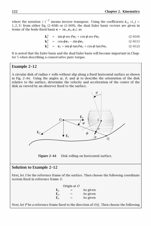
122 Chapter 2. Kinematics
where the notation ·−T means inverse transpose. Using the coefficients kij (i, j =1,2,3) from either Eq. (2–608) or (2–609), the dual Euler basis vectors are given interms of the body-fixed basis e = e1,e2,e3 as
k∗1 = sinφ secθe2 + cosφ secθe3 (2–610)
k∗2 = cosφe2 − sinφe3 (2–611)
k∗3 = e1 + sinφ tanθe2 + cosφ tanθe3 (2–612)
It is noted that the Euler basis and the dual Euler basis will become important in Chap-ter 5 when describing a conservative pure torque.
Example 2–12
A circular disk of radius r rolls without slip along a fixed horizontal surface as shownin Fig. 2–44. Using the angles ψ, θ, and φ to describe the orientation of the diskrelative to the surface, determine the velocity and acceleration of the center of thedisk as viewed by an observer fixed to the surface.
Ex
EyEz
r
CO
P Q
θ
ψ
φ
Figure 2–44 Disk rolling on horizontal surface.
Solution to Example 2–12
First, let S be the reference frame of the surface. Then choose the following coordinatesystem fixed in reference frame S:
Origin at OEx = As givenEy = As givenEz = As given
Next, let P be a reference frame fixed to the direction ofOQ. Then choose the following
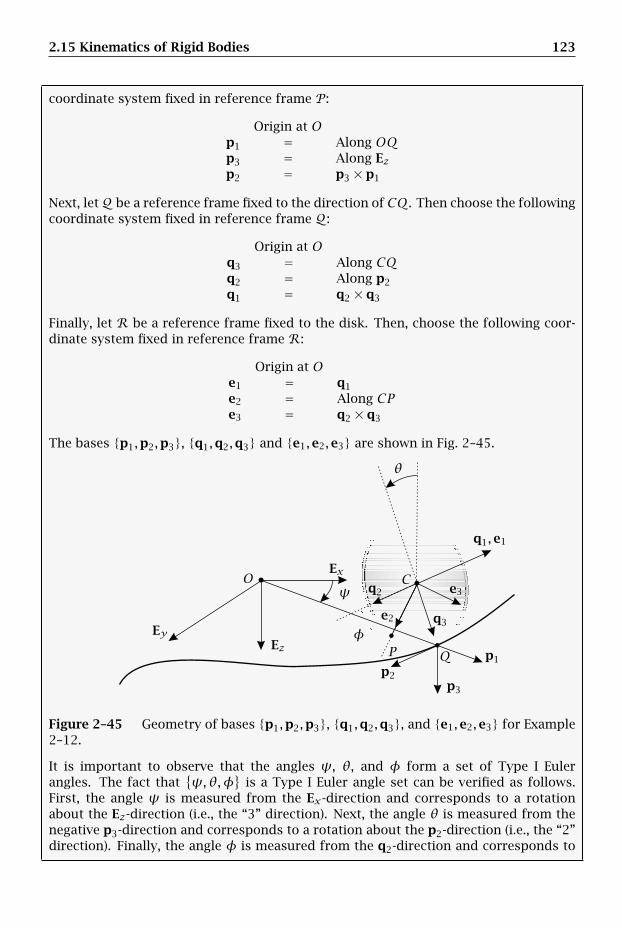
2.15 Kinematics of Rigid Bodies 123
coordinate system fixed in reference frame P:
Origin at Op1 = Along OQp3 = Along Ezp2 = p3 × p1
Next, letQ be a reference frame fixed to the direction of CQ. Then choose the followingcoordinate system fixed in reference frame Q:
Origin at Oq3 = Along CQq2 = Along p2q1 = q2 × q3
Finally, let R be a reference frame fixed to the disk. Then, choose the following coor-dinate system fixed in reference frame R:
Origin at Oe1 = q1e2 = Along CPe3 = q2 × q3
The bases p1,p2,p3, q1,q2,q3 and e1,e2,e3 are shown in Fig. 2–45.
q1,e1
e2
e3
Ex
EyEz
p1p2
p3
q2
q3
CO
P Q
θ
ψ
φ
Figure 2–45 Geometry of bases p1,p2,p3, q1,q2,q3, and e1,e2,e3 for Example2–12.
It is important to observe that the angles ψ, θ, and φ form a set of Type I Eulerangles. The fact that
ψ,θ,φ
is a Type I Euler angle set can be verified as follows.
First, the angle ψ is measured from the Ex-direction and corresponds to a rotationabout the Ez-direction (i.e., the “3” direction). Next, the angle θ is measured from thenegative p3-direction and corresponds to a rotation about the p2-direction (i.e., the “2”direction). Finally, the angle φ is measured from the q2-direction and corresponds to
124 Chapter 2. Kinematics
a rotation about the q1-direction (i.e., the “1” direction). Therefore, the setψ,θ,φ
is
a “3-2-1” Euler angle sequence, i.e.,ψ,θ,φ
is a set of Type I Euler angles.
Now, becauseψ,θ,φ
is a set of Type I Euler angles, we have the following:
SωP = ψp3 (2–613)PωQ = θq2 (2–614)QωR = φe1 (2–615)
where SωP is the angular velocity of P in S, PωQ is the angular velocity of Q in P, andQωR is the angular velocity of R in Q. The angular velocity of the disk as viewed byan observer fixed to the surface is then obtained from the angular velocity additiontheorem as
SωR = SωP + PωQ + QωR = ψp3 + θq2 + φe1 (2–616)
where we note thatp3,q2,e1
is the Euler basis. Furthermore, the position of point C
relative to point Q is given in terms of the basis q1,q2,q3 as
rC − rQ = −rq3 (2–617)
Now, because the disk rolls without slip along a fixed surface, we have
SvRQ = 0 (2–618)
The velocity of the center of the disk as viewed by an observer fixed to the surface isthen given from Eq. (2–517) as
SvC = SvRQ + SωR × (rC − rQ) (2–619)
Substituting the results of Eqs. (2–616), (2–617), and (2–618) into Eq. (2–619), we obtain
SvC = (ψp3 + θq2 + φe1)× (−rq3) (2–620)
Equation (2–620) simplifies to
SvC = −rψp3 × q3 − r θq1 + rφq2 (2–621)
Now, consistent with the definition of the Type I Euler angle sequence, we have
p3 = − sinθq1 + cosθq3 (2–622)
Substituting the result of Eq. (2–622) into Eq. (2–621), we obtain
SvC = −rψ(− sinθq1 + cosθq3)× q3 − r θq1 + rφq2
= −rψ sinθq2 − r θq1 + rφq2
(2–623)
Rearranging Eq. (2–623), the velocity of the center of the disk as viewed by an observerfixed to the surface is given as
SvC = −r θq1 + (rφ− rψ sinθ)q2 (2–624)
The acceleration of the center of the disk as viewed by an observer fixed to thesurface is obtained as follows. First, we see from Eq. (2–624) that SvC is expressed in
2.15 Kinematics of Rigid Bodies 125
the basis q1,q2,q3 and q1,q2,q3 is fixed in reference frame Q. Consequently, it ismost convenient to determine SaC by applying the rate of change transport theorembetween reference frames Q and S, i.e.,
SaC =Sddt
(SvC
)=Qddt
(SvC
)+ SωQ × SvC (2–625)
Now the angular velocity of Q in S is given as
SωQ = SωP + PωQ = ψp3 + θq2 (2–626)
Next, we have
Qddt
(SvC
)= −r θq1 + (rφ− rψ sinθ − rψθ cosθ)q2 (2–627)
SωQ × SvC = (ψp3 + θq2)×[−r θq1 + (rφ− rψ sinθ)q2
](2–628)
Computing the vector product in Eq. (2–628), we obtain
SωQ × SvC = −rψθp3 × q1 + rψ(φ− rψ sinθ)p3 × q2 + r θ2q3 (2–629)
Using the expression for p3 from Eq. (2–622), the quantities p3 × q1 and p3 × q2 aregiven as
p3 × q1 = (− sinθq1 + cosθq3)× q1 = cosθq2 (2–630)
p3 × q2 = (− sinθq1 + cosθq3)× q2 = − sinθq3 − cosθq1 (2–631)
Substituting the results of Eqs. (2–630) and (2–631) into (2–629) gives
SωQ × SvC = −rψθ cosθq2 − rψ(φ− ψ sinθ)(sinθq3 + cosθq1)+ r θ2q3 (2–632)
Simplifying Eq. (2–632), we obtain
SωQ × SvC = −rψ(φ− ψ sinθ) cosθq1 − rψθ cosθq2
+[r θ2 − rψ(φ− rψ sinθ) sinθ
]q3
(2–633)
Adding Eqs. (2–627) and (2–633), the acceleration of the center of the disk as viewedby an observer fixed to the surface is given as
SaC = −[r θ + rψ(φ− ψ sinθ) cosθ
]q1
+ (rφ− rψ sinθ − 2rψθ cosθ)q2
+[r θ2 − rψ(φ− ψ sinθ) sinθ
]q3
(2–634)
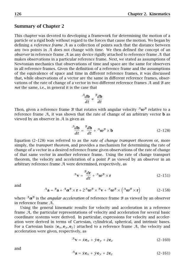
126 Chapter 2. Kinematics
Summary of Chapter 2
This chapter was devoted to developing a framework for determining the motion of aparticle or a rigid body without regard to the forces that cause the motion. We began bydefining a reference frame A as a collection of points such that the distance betweenany two points in A does not change with time. We then defined the concept of anobserver in reference frameA as any device rigidly attached to reference frameA thatmakes observations in a particular reference frame. Next, we stated as assumptions ofNewtonian mechanics that observations of time and space are the same for observersin all reference frames. Given the definition of a reference frame and the assumptionsof the equivalence of space and time in different reference frames, it was discussedthat, while observations of a vector are the same in different reference frames, obser-vations of the rate of change of a vector in two different reference frames A and B arenot the same, i.e., in general it is the case that
Adbdt
≠Bdbdt
Then, given a reference frame B that rotates with angular velocity AωB relative to areference frame A, it was shown that the rate of change of an arbitrary vector b asviewed by an observer in A is given as
Adbdt
=Bdbdt
+AωB × b (2–128)
Equation (2–128) was referred to as the rate of change transport theorem or, moresimply, the transport theorem, and provides a mechanism for determining the rate ofchange of a vector in a desired reference frame given observations of the rate of changeof that same vector in another reference frame. Using the rate of change transporttheorem, the velocity and acceleration of a point P as viewed by an observer in anarbitrary reference frame A were determined, respectively, as
Av =Bdrdt+AωB × r (2–151)
andAa = Ba+AαB × r+ 2AωB × Bv+AωB ×
(AωB × r
)(2–158)
where AαB is the angular acceleration of reference frame B as viewed by an observerin reference frame A.
Using the general kinematic results for velocity and acceleration in a referenceframe A, the particular representations of velocity and acceleration for several basiccoordinate systems were derived. In particular, expressions for velocity and acceler-ation were derived in terms of Cartesian, cylindrical, spherical, and intrinsic bases.For a Cartesian basis ex,ey,ez attached to a reference frame A, the velocity andacceleration were given, respectively, as
Av = xex + yey + zez (2–160)
andAa = xex + yey + zez (2–161)
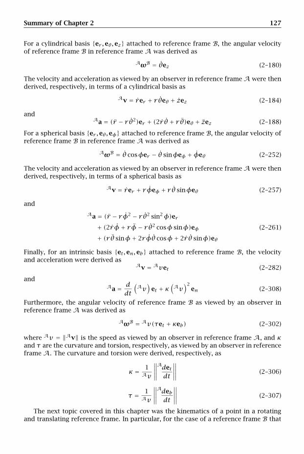
Summary of Chapter 2 127
For a cylindrical basis er ,eθ,ez attached to reference frame B, the angular velocityof reference frame B in reference frame A was derived as
AωB = θez (2–180)
The velocity and acceleration as viewed by an observer in reference frameA were thenderived, respectively, in terms of a cylindrical basis as
Av = rer + r θeθ + zez (2–184)
andAa = (r − r θ2)er + (2r θ + r θ)eθ + zez (2–188)
For a spherical basis er ,eθ,eφ attached to reference frame B, the angular velocity ofreference frame B in reference frame A was derived as
AωB = θ cosφer − θ sinφeφ + φeθ (2–252)
The velocity and acceleration as viewed by an observer in reference frameA were thenderived, respectively, in terms of a spherical basis as
Av = rer + rφeφ + r θ sinφeθ (2–257)
and
Aa = (r − rφ2 − r θ2 sin2φ)er+ (2r φ+ rφ− r θ2 cosφ sinφ)eφ+ (r θ sinφ+ 2rφθ cosφ+ 2r θ sinφ)eθ
(2–261)
Finally, for an intrinsic basis et,en,eb attached to reference frame B, the velocityand acceleration were derived as
Av = Avet (2–282)
andAa = d
dt
(Av
)et + κ
(Av
)2en (2–308)
Furthermore, the angular velocity of reference frame B as viewed by an observer inreference frame A was derived as
AωB = Av(τet + κeb) (2–302)
where Av = ‖Av‖ is the speed as viewed by an observer in reference frame A, and κand τ are the curvature and torsion, respectively, as viewed by an observer in referenceframe A. The curvature and torsion were derived, respectively, as
κ = 1Av
∥∥∥∥∥Adetdt
∥∥∥∥∥ (2–306)
τ = 1Av
∥∥∥∥∥Adebdt
∥∥∥∥∥ (2–307)
The next topic covered in this chapter was the kinematics of a point in a rotatingand translating reference frame. In particular, for the case of a reference frame B that
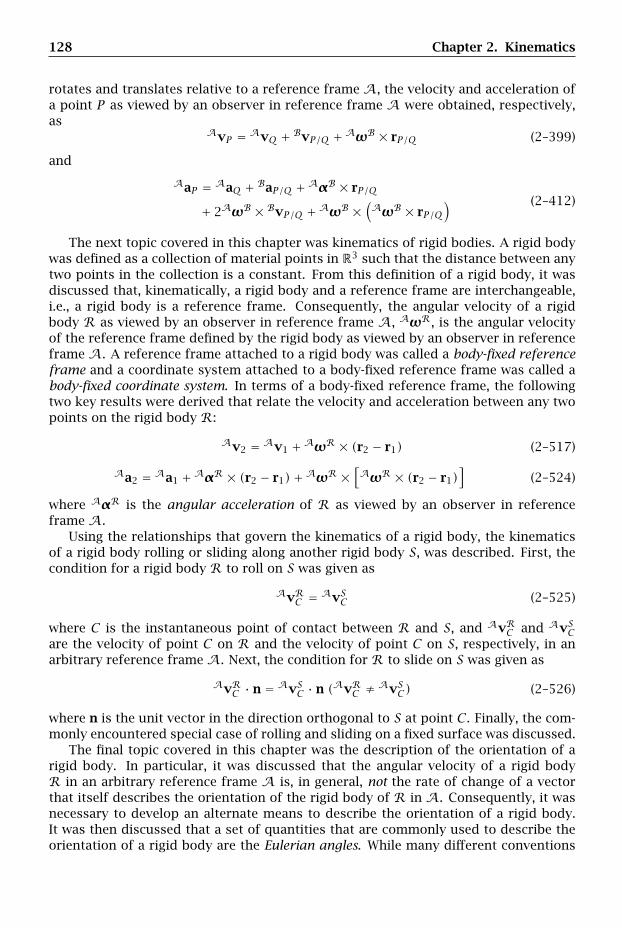
128 Chapter 2. Kinematics
rotates and translates relative to a reference frame A, the velocity and acceleration ofa point P as viewed by an observer in reference frame A were obtained, respectively,as
AvP = AvQ + BvP/Q +AωB × rP/Q (2–399)
and
AaP = AaQ + BaP/Q +AαB × rP/Q
+ 2AωB × BvP/Q +AωB ×(AωB × rP/Q
) (2–412)
The next topic covered in this chapter was kinematics of rigid bodies. A rigid bodywas defined as a collection of material points in R3 such that the distance between anytwo points in the collection is a constant. From this definition of a rigid body, it wasdiscussed that, kinematically, a rigid body and a reference frame are interchangeable,i.e., a rigid body is a reference frame. Consequently, the angular velocity of a rigidbody R as viewed by an observer in reference frame A, AωR, is the angular velocityof the reference frame defined by the rigid body as viewed by an observer in referenceframe A. A reference frame attached to a rigid body was called a body-fixed referenceframe and a coordinate system attached to a body-fixed reference frame was called abody-fixed coordinate system. In terms of a body-fixed reference frame, the followingtwo key results were derived that relate the velocity and acceleration between any twopoints on the rigid body R:
Av2 = Av1 +AωR × (r2 − r1) (2–517)
Aa2 = Aa1 +AαR × (r2 − r1)+AωR ×[AωR × (r2 − r1)
](2–524)
where AαR is the angular acceleration of R as viewed by an observer in referenceframe A.
Using the relationships that govern the kinematics of a rigid body, the kinematicsof a rigid body rolling or sliding along another rigid body S, was described. First, thecondition for a rigid body R to roll on S was given as
AvRC = AvSC (2–525)
where C is the instantaneous point of contact between R and S, and AvRC and AvSCare the velocity of point C on R and the velocity of point C on S, respectively, in anarbitrary reference frame A. Next, the condition for R to slide on S was given as
AvRC · n = AvSC · n (AvRC ≠AvSC) (2–526)
where n is the unit vector in the direction orthogonal to S at point C . Finally, the com-monly encountered special case of rolling and sliding on a fixed surface was discussed.
The final topic covered in this chapter was the description of the orientation of arigid body. In particular, it was discussed that the angular velocity of a rigid bodyR in an arbitrary reference frame A is, in general, not the rate of change of a vectorthat itself describes the orientation of the rigid body of R in A. Consequently, it wasnecessary to develop an alternate means to describe the orientation of a rigid body.It was then discussed that a set of quantities that are commonly used to describe theorientation of a rigid body are the Eulerian angles. While many different conventions
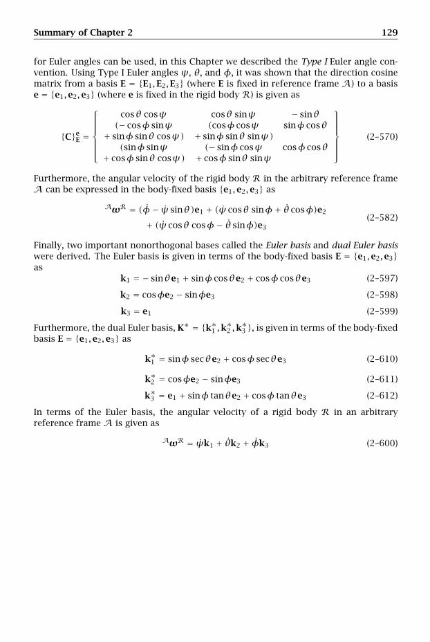
Summary of Chapter 2 129
for Euler angles can be used, in this Chapter we described the Type I Euler angle con-vention. Using Type I Euler angles ψ, θ, and φ, it was shown that the direction cosinematrix from a basis E = E1,E2,E3 (where E is fixed in reference frame A) to a basise = e1,e2,e3 (where e is fixed in the rigid body R) is given as
CeE =
⎧⎪⎪⎪⎪⎪⎨⎪⎪⎪⎪⎪⎩
cosθ cosψ cosθ sinψ − sinθ(− cosφ sinψ (cosφ cosψ sinφ cosθ
+ sinφ sinθ cosψ) + sinφ sinθ sinψ)(sinφ sinψ (− sinφ cosψ cosφ cosθ
+ cosφ sinθ cosψ) + cosφ sinθ sinψ
⎫⎪⎪⎪⎪⎪⎬⎪⎪⎪⎪⎪⎭
(2–570)
Furthermore, the angular velocity of the rigid body R in the arbitrary reference frameA can be expressed in the body-fixed basis e1,e2,e3 as
AωR = (φ− ψ sinθ)e1 + (ψ cosθ sinφ+ θ cosφ)e2
+ (ψ cosθ cosφ− θ sinφ)e3(2–582)
Finally, two important nonorthogonal bases called the Euler basis and dual Euler basiswere derived. The Euler basis is given in terms of the body-fixed basis E = e1,e2,e3as
k1 = − sinθe1 + sinφ cosθe2 + cosφ cosθe3 (2–597)
k2 = cosφe2 − sinφe3 (2–598)
k3 = e1 (2–599)
Furthermore, the dual Euler basis, K∗ = k∗1 ,k∗2 ,k∗3 , is given in terms of the body-fixedbasis E = e1,e2,e3 as
k∗1 = sinφ secθe2 + cosφ secθe3 (2–610)
k∗2 = cosφe2 − sinφe3 (2–611)
k∗3 = e1 + sinφ tanθe2 + cosφ tanθe3 (2–612)
In terms of the Euler basis, the angular velocity of a rigid body R in an arbitraryreference frame A is given as
AωR = ψk1 + θk2 + φk3 (2–600)
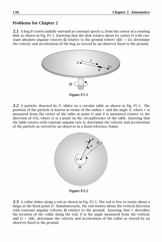
130 Chapter 2. Kinematics
Problems for Chapter 2
2.1 A bug B crawls radially outward at constant speed v0 from the center of a rotatingdisk as shown in Fig. P2-1. Knowing that the disk rotates about its center O with con-stant absolute angular velocity Ω relative to the ground (where ‖Ω‖ = Ω), determinethe velocity and acceleration of the bug as viewed by an observer fixed to the ground.
r
v0B
O
Ω
Figure P2-1
2.2 A particle, denoted by P , slides on a circular table as shown in Fig. P2-2. Theposition of the particle is known in terms of the radius r and the angle θ, where r ismeasured from the center of the table at point O and θ is measured relative to thedirection of OQ, where Q is a point on the circumference of the table. Knowing thatthe table rotates with constant angular rate Ω, determine the velocity and accelerationof the particle as viewed by an observer in a fixed reference frame.
r
O
PQ
θ
Ω
Figure P2-2
2.3 A collar slides along a rod as shown in Fig. P2-3. The rod is free to rotate about ahinge at the fixed point O. Simultaneously, the rod rotates about the vertical directionwith constant angular velocity Ω relative to the ground. Knowing that r describesthe location of the collar along the rod, θ is the angle measured from the vertical,and Ω = ‖Ω‖, determine the velocity and acceleration of the collar as viewed by anobserver fixed to the ground.
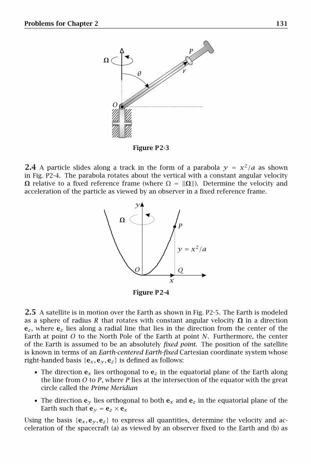
Problems for Chapter 2 131
r
O
P
θ
Ω
Figure P2-3
2.4 A particle slides along a track in the form of a parabola y = x2/a as shownin Fig. P2-4. The parabola rotates about the vertical with a constant angular velocityΩ relative to a fixed reference frame (where Ω = ‖Ω‖). Determine the velocity andacceleration of the particle as viewed by an observer in a fixed reference frame.
y = x2/a
x
y
O
P
Q
Ω
Figure P2-4
2.5 A satellite is in motion over the Earth as shown in Fig. P2-5. The Earth is modeledas a sphere of radius R that rotates with constant angular velocity Ω in a directionez, where ez lies along a radial line that lies in the direction from the center of theEarth at point O to the North Pole of the Earth at point N. Furthermore, the centerof the Earth is assumed to be an absolutely fixed point. The position of the satelliteis known in terms of an Earth-centered Earth-fixed Cartesian coordinate system whoseright-handed basis ex,ey,ez is defined as follows:
• The direction ex lies orthogonal to ez in the equatorial plane of the Earth alongthe line from O to P , where P lies at the intersection of the equator with the greatcircle called the Prime Meridian
• The direction ey lies orthogonal to both ex and ez in the equatorial plane of theEarth such that ey = ez × ex
Using the basis ex,ey,ez to express all quantities, determine the velocity and ac-celeration of the spacecraft (a) as viewed by an observer fixed to the Earth and (b) as

132 Chapter 2. Kinematics
viewed by an observer in a fixed inertial reference frame.
×Prime Meridian
Spacecraft
Equator
exey
ez
rN
O
P Q
Ω
Figure P2-5
2.6 An arm of length L is hinged at one of its ends at point O to a vertical shaft asshown in Fig. P2-6. The shaft rotates with constant angular velocity Ω relative to theground. Assuming that the arm is free to pivot about the point O and θ describes theangle of the shaft from the downward direction, determine the velocity and accelera-tion of the free end of the arm (point P ) as viewed by an observer fixed to the ground.
L
O
P
θ
Ω
Figure P2-6
2.7 A circular disk of radius R rolls without slip along a horizontal surface as shownin Fig. P2-7. Knowing that point P is located on the edge of the disk and θ is theangle formed by the vertical and the direction OP (where O is the center of the disk),determine the following quantities relative to an observer fixed in the ground: (a) thevelocity of point P and (b) the acceleration of point P .
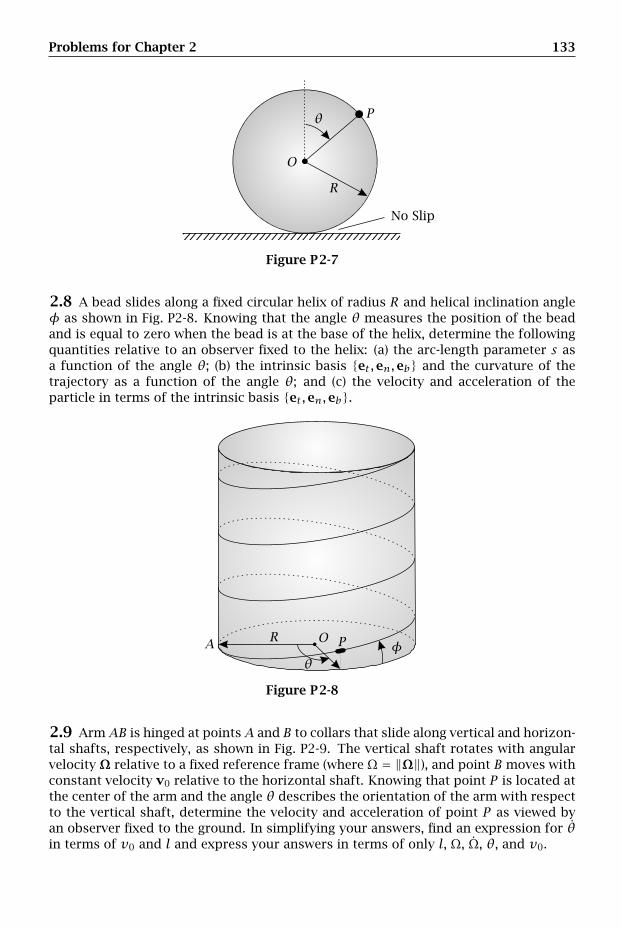
Problems for Chapter 2 133
No Slip
O
P
R
θ
Figure P2-7
2.8 A bead slides along a fixed circular helix of radius R and helical inclination angleφ as shown in Fig. P2-8. Knowing that the angle θ measures the position of the beadand is equal to zero when the bead is at the base of the helix, determine the followingquantities relative to an observer fixed to the helix: (a) the arc-length parameter s asa function of the angle θ; (b) the intrinsic basis et,en,eb and the curvature of thetrajectory as a function of the angle θ; and (c) the velocity and acceleration of theparticle in terms of the intrinsic basis et,en,eb.
A O PR
θφ
Figure P2-8
2.9 ArmAB is hinged at pointsA and B to collars that slide along vertical and horizon-tal shafts, respectively, as shown in Fig. P2-9. The vertical shaft rotates with angularvelocity Ω relative to a fixed reference frame (where Ω = ‖Ω‖), and point B moves withconstant velocity v0 relative to the horizontal shaft. Knowing that point P is located atthe center of the arm and the angle θ describes the orientation of the arm with respectto the vertical shaft, determine the velocity and acceleration of point P as viewed byan observer fixed to the ground. In simplifying your answers, find an expression for θin terms of v0 and l and express your answers in terms of only l, Ω, Ω, θ, and v0.
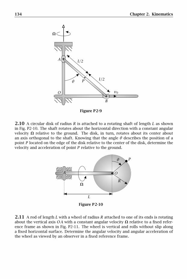
134 Chapter 2. Kinematics
l/2
l/2
v0
A
B
O
Pθ
Ω
Figure P2-9
2.10 A circular disk of radius R is attached to a rotating shaft of length L as shownin Fig. P2-10. The shaft rotates about the horizontal direction with a constant angularvelocity Ω relative to the ground. The disk, in turn, rotates about its center aboutan axis orthogonal to the shaft. Knowing that the angle θ describes the position of apoint P located on the edge of the disk relative to the center of the disk, determine thevelocity and acceleration of point P relative to the ground.
A
L
O
P
R
θ
Ω
Figure P2-10
2.11 A rod of length L with a wheel of radius R attached to one of its ends is rotatingabout the vertical axis OA with a constant angular velocity Ω relative to a fixed refer-ence frame as shown in Fig. P2-11. The wheel is vertical and rolls without slip alonga fixed horizontal surface. Determine the angular velocity and angular acceleration ofthe wheel as viewed by an observer in a fixed reference frame.
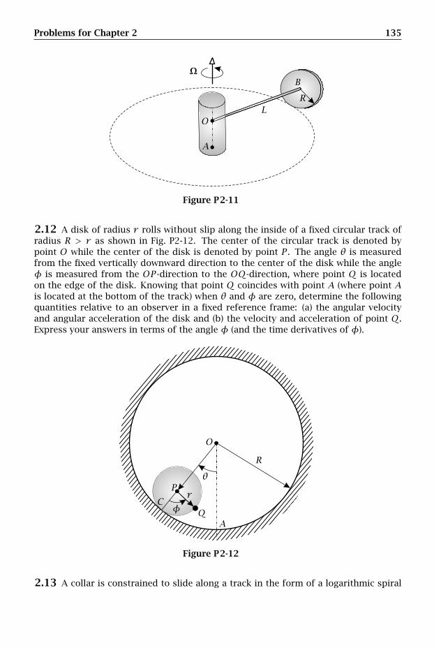
Problems for Chapter 2 135
A
B
LO
R
Ω
Figure P2-11
2.12 A disk of radius r rolls without slip along the inside of a fixed circular track ofradius R > r as shown in Fig. P2-12. The center of the circular track is denoted bypoint O while the center of the disk is denoted by point P . The angle θ is measuredfrom the fixed vertically downward direction to the center of the disk while the angleφ is measured from the OP -direction to the OQ-direction, where point Q is locatedon the edge of the disk. Knowing that point Q coincides with point A (where point Ais located at the bottom of the track) when θ and φ are zero, determine the followingquantities relative to an observer in a fixed reference frame: (a) the angular velocityand angular acceleration of the disk and (b) the velocity and acceleration of point Q.Express your answers in terms of the angle φ (and the time derivatives of φ).
r
A
C
O
P
Q
R
θ
φ
Figure P2-12
2.13 A collar is constrained to slide along a track in the form of a logarithmic spiral
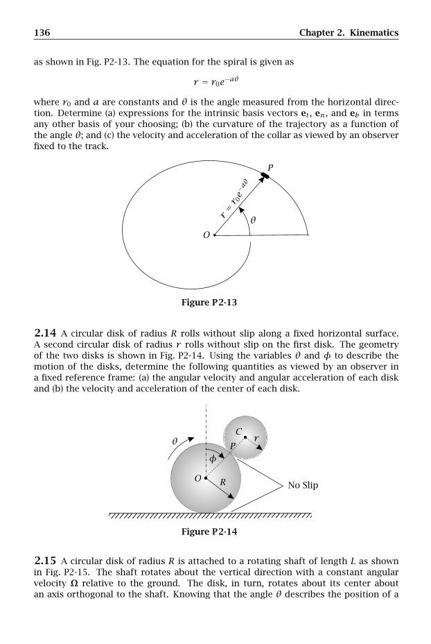
136 Chapter 2. Kinematics
as shown in Fig. P2-13. The equation for the spiral is given as
r = r0e−aθ
where r0 and a are constants and θ is the angle measured from the horizontal direc-tion. Determine (a) expressions for the intrinsic basis vectors et , en, and eb in termsany other basis of your choosing; (b) the curvature of the trajectory as a function ofthe angle θ; and (c) the velocity and acceleration of the collar as viewed by an observerfixed to the track.
r= r
0e−aθ
O
P
θ
Figure P2-13
2.14 A circular disk of radius R rolls without slip along a fixed horizontal surface.A second circular disk of radius r rolls without slip on the first disk. The geometryof the two disks is shown in Fig. P2-14. Using the variables θ and φ to describe themotion of the disks, determine the following quantities as viewed by an observer ina fixed reference frame: (a) the angular velocity and angular acceleration of each diskand (b) the velocity and acceleration of the center of each disk.
No Slip
rC
O
P
R
θ
φ
Figure P2-14
2.15 A circular disk of radius R is attached to a rotating shaft of length L as shownin Fig. P2-15. The shaft rotates about the vertical direction with a constant angularvelocity Ω relative to the ground. The disk, in turn, rotates about its center aboutan axis orthogonal to the shaft. Knowing that the angle θ describes the position of a
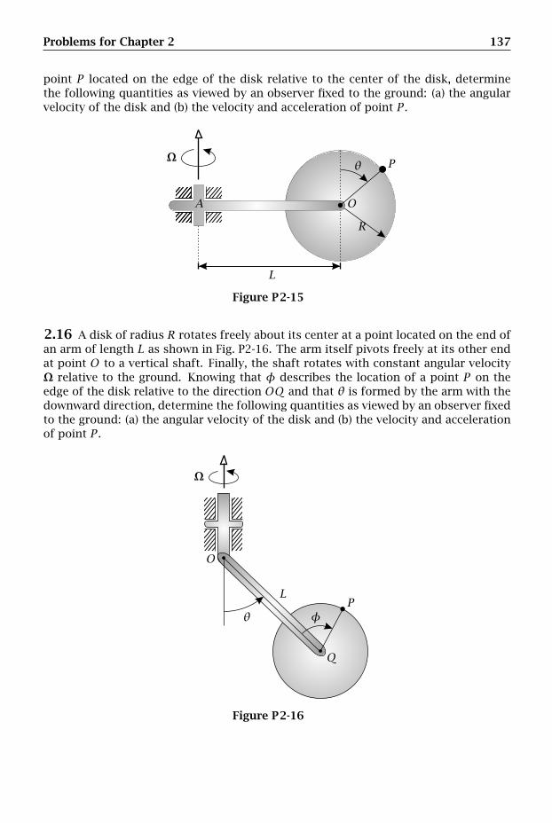
Problems for Chapter 2 137
point P located on the edge of the disk relative to the center of the disk, determinethe following quantities as viewed by an observer fixed to the ground: (a) the angularvelocity of the disk and (b) the velocity and acceleration of point P .
A
L
O
P
R
θΩ
Figure P2-15
2.16 A disk of radius R rotates freely about its center at a point located on the end ofan arm of length L as shown in Fig. P2-16. The arm itself pivots freely at its other endat point O to a vertical shaft. Finally, the shaft rotates with constant angular velocityΩ relative to the ground. Knowing that φ describes the location of a point P on theedge of the disk relative to the direction OQ and that θ is formed by the arm with thedownward direction, determine the following quantities as viewed by an observer fixedto the ground: (a) the angular velocity of the disk and (b) the velocity and accelerationof point P .
L
O
P
Q
θ φ
Ω
Figure P2-16
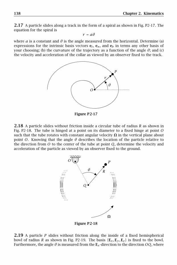
138 Chapter 2. Kinematics
2.17 A particle slides along a track in the form of a spiral as shown in Fig. P2-17. Theequation for the spiral is
r = aθwhere a is a constant and θ is the angle measured from the horizontal. Determine (a)expressions for the intrinsic basis vectors et , en, and eb in terms any other basis ofyour choosing; (b) the curvature of the trajectory as a function of the angle θ; and (c)the velocity and acceleration of the collar as viewed by an observer fixed to the track.
r
O
P
θ
Figure P2-17
2.18 A particle slides without friction inside a circular tube of radius R as shown inFig. P2-18. The tube is hinged at a point on its diameter to a fixed hinge at point Osuch that the tube rotates with constant angular velocity Ω in the vertical plane aboutpoint O. Knowing that the angle θ describes the location of the particle relative tothe direction from O to the center of the tube at point Q, determine the velocity andacceleration of the particle as viewed by an observer fixed to the ground.
O P
Q
Rθ
Ω
Figure P2-18
2.19 A particle P slides without friction along the inside of a fixed hemisphericalbowl of radius R as shown in Fig. P2-19. The basis Ex,Ey,Ez is fixed to the bowl.Furthermore, the angle θ is measured from the Ex-direction to the direction OQ, where

Problems for Chapter 2 139
point Q lies on the rim of the bowl while the angle φ is measured from the OQ-direction to the position of the particle. Determine the velocity and acceleration of theparticle as viewed by an observer fixed to the bowl. Hint: Express the position in termsof a spherical basis that is fixed to the direction OP ; then determine the velocity andacceleration as viewed by an observer fixed to the bowl in terms of this spherical basis.
Ex
Ey
Ez
O
P
Q
R
θφ
Figure P2-19
2.20 A particle P slides along a circular table as shown in Fig. P2-20. The table isrigidly attached to two shafts such that the shafts and table rotate with angular velocityΩ about an axis along the direction of the shafts. Knowing that the position of theparticle is given in terms of a polar coordinate system relative to the table, determine(a) the angular velocity of the table as viewed by an observer fixed to the ground, (b)the velocity and acceleration of the particle as viewed by an observer fixed to the table,and (c) the velocity and acceleration of the particle as viewed by an observer fixed tothe ground.
r
A
B
OP
θ
Ω
Figure P2-20
2.21 A slender rod of length l is hinged to a collar as shown in Fig. P2-21. Thecollar slides freely along a fixed horizontal track. Knowing that x is the horizontaldisplacement of the collar and that θ describes the orientation of the rod relative tothe vertical direction, determine the velocity and acceleration of the free end of therod as viewed by an observer fixed to the track.
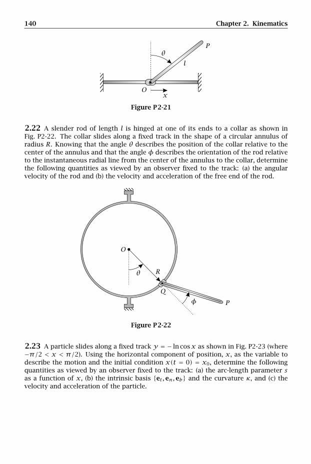
140 Chapter 2. Kinematics
l
xO
Pθ
Figure P2-21
2.22 A slender rod of length l is hinged at one of its ends to a collar as shown inFig. P2-22. The collar slides along a fixed track in the shape of a circular annulus ofradius R. Knowing that the angle θ describes the position of the collar relative to thecenter of the annulus and that the angle φ describes the orientation of the rod relativeto the instantaneous radial line from the center of the annulus to the collar, determinethe following quantities as viewed by an observer fixed to the track: (a) the angularvelocity of the rod and (b) the velocity and acceleration of the free end of the rod.
O
P
Q
Rθ
φ
Figure P2-22
2.23 A particle slides along a fixed track y = − ln cosx as shown in Fig. P2-23 (where−π/2 < x < π/2). Using the horizontal component of position, x, as the variable todescribe the motion and the initial condition x(t = 0) = x0, determine the followingquantities as viewed by an observer fixed to the track: (a) the arc-length parameter sas a function of x, (b) the intrinsic basis et,en,eb and the curvature κ, and (c) thevelocity and acceleration of the particle.
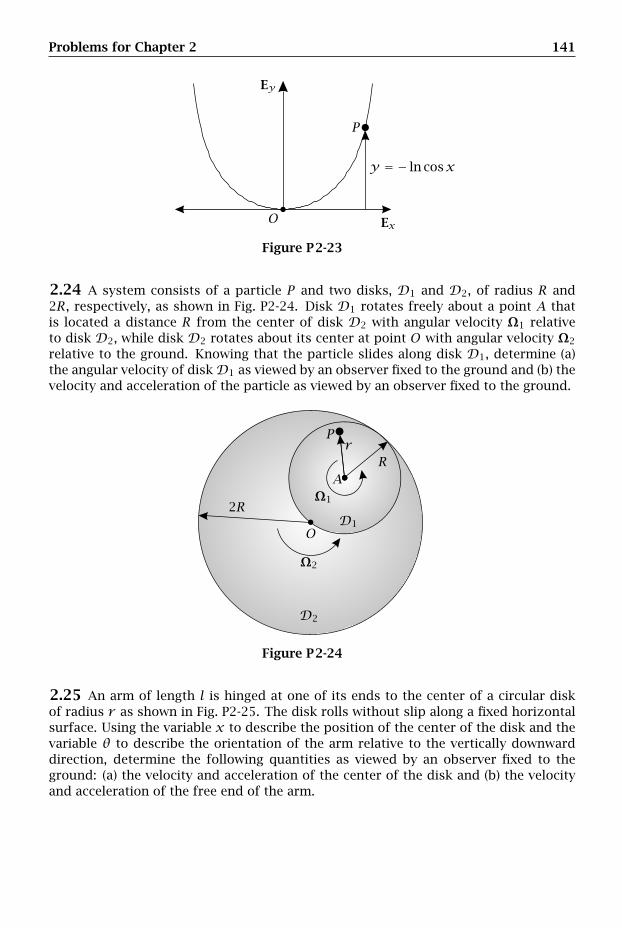
Problems for Chapter 2 141
y = − ln cosx
Ex
Ey
O
P
Figure P2-23
2.24 A system consists of a particle P and two disks, D1 and D2, of radius R and2R, respectively, as shown in Fig. P2-24. Disk D1 rotates freely about a point A thatis located a distance R from the center of disk D2 with angular velocity Ω1 relativeto disk D2, while disk D2 rotates about its center at point O with angular velocity Ω2
relative to the ground. Knowing that the particle slides along disk D1, determine (a)the angular velocity of diskD1 as viewed by an observer fixed to the ground and (b) thevelocity and acceleration of the particle as viewed by an observer fixed to the ground.
D1
D2
r
A
O
P
R
2RΩ1
Ω2
Figure P2-24
2.25 An arm of length l is hinged at one of its ends to the center of a circular diskof radius r as shown in Fig. P2-25. The disk rolls without slip along a fixed horizontalsurface. Using the variable x to describe the position of the center of the disk and thevariable θ to describe the orientation of the arm relative to the vertically downwarddirection, determine the following quantities as viewed by an observer fixed to theground: (a) the velocity and acceleration of the center of the disk and (b) the velocityand acceleration of the free end of the arm.
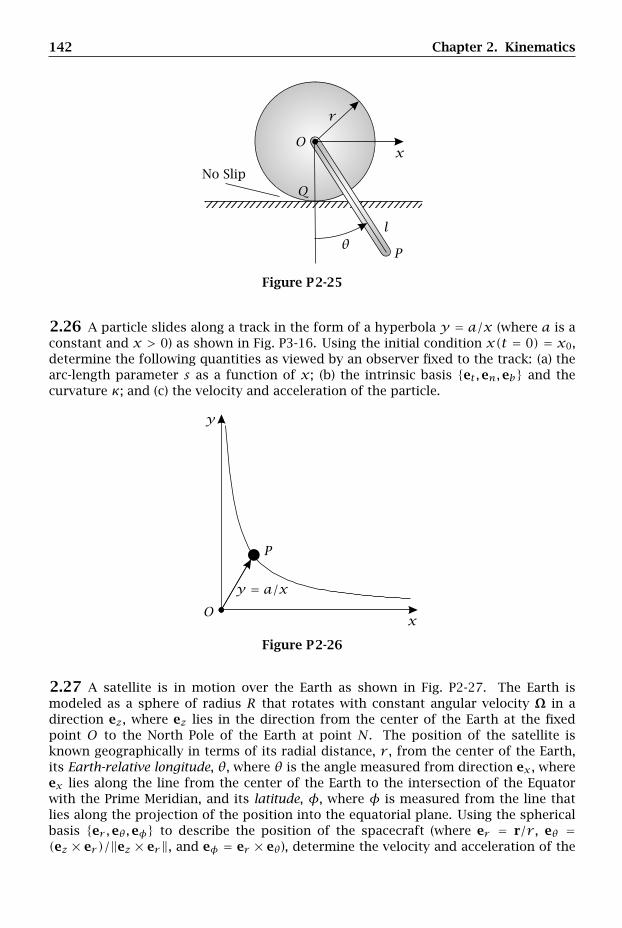
142 Chapter 2. Kinematics
No Slip
l
r
xO
P
Q
θ
Figure P2-25
2.26 A particle slides along a track in the form of a hyperbola y = a/x (where a is aconstant and x > 0) as shown in Fig. P3-16. Using the initial condition x(t = 0) = x0,determine the following quantities as viewed by an observer fixed to the track: (a) thearc-length parameter s as a function of x; (b) the intrinsic basis et,en,eb and thecurvature κ; and (c) the velocity and acceleration of the particle.
y = a/x
x
y
O
P
Figure P2-26
2.27 A satellite is in motion over the Earth as shown in Fig. P2-27. The Earth ismodeled as a sphere of radius R that rotates with constant angular velocity Ω in adirection ez, where ez lies in the direction from the center of the Earth at the fixedpoint O to the North Pole of the Earth at point N. The position of the satellite isknown geographically in terms of its radial distance, r , from the center of the Earth,its Earth-relative longitude, θ, where θ is the angle measured from direction ex , whereex lies along the line from the center of the Earth to the intersection of the Equatorwith the Prime Meridian, and its latitude, φ, where φ is measured from the line thatlies along the projection of the position into the equatorial plane. Using the sphericalbasis er ,eθ,eφ to describe the position of the spacecraft (where er = r/r , eθ =(ez × er )/‖ez × er‖, and eφ = er × eθ), determine the velocity and acceleration of the
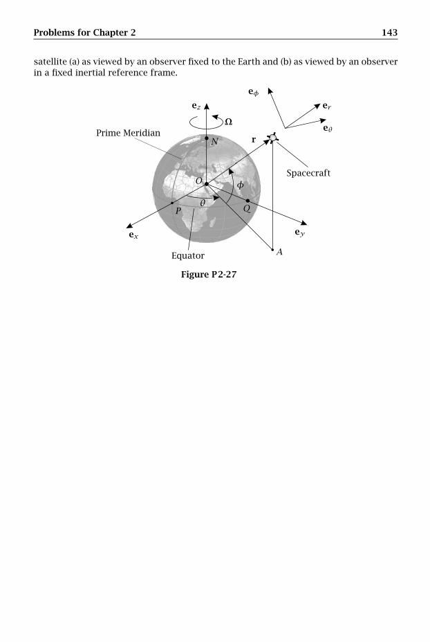
Problems for Chapter 2 143
satellite (a) as viewed by an observer fixed to the Earth and (b) as viewed by an observerin a fixed inertial reference frame.
×Prime Meridian
Spacecraft
Equator
er
eθ
eφ
ex ey
ez
r
A
N
O
P Qθ
φ
Ω
Figure P2-27


Chapter 3
Kinetics of Particles
If I have seen further it is by standing upon the shoulders of giants.
- Sir Isaac Newton (1642–1727)British Physicist and Mathematician
Until now, we have been concerned with the kinematics of particles where the ob-jective has been to determine the motion of a particle or rigid body without regard tothe cause of the motion. Clearly in any physical system motion cannot occur withoutthe application of some kind of external stimulus. In particular, in order for a particleto accelerate, it is necessary to apply a force to the particle. In order to study themotion that results from the application of a force (or, in general, the application ofmultiple forces) to a particle, it is necessary to study the kinetics of the particle. Theobjective of kinetics is threefold: (1) to describe quantitatively the forces that act on aparticle; (2) to determine the motion that results from the application of these forcesusing postulated laws of physics; and (3) to analyze the motion.
The first topic in this chapter is the development of models for forces that arecommonly used in dynamics. In particular, models are developed for contact forces,spring forces, and gravitational forces. These models will be used throughout theremainder of this book when solving problems.
The next topic in this chapter covers Newton’s laws, which are the fundamentalpostulates that govern the nonrelativistic motion of particles. A framework is thenestablished for the systematic application of Newton’s laws. Several example problemsare then solved using Newton’s laws.
The next topics in this chapter are linear momentum and angular momentum of aparticle. First, the definition of linear momentum of a particle is established. Using thedefinition of linear momentum, the principle of linear impulse and linear momentumfor a particle is derived. Next, the definition of the moment of a force and the angularmomentum of a particle are established. Using the definition of angular momentum,the principle of angular impulse and angular momentum for a particle is derived.
The final topics covered in this chapter are the power, work, and energy of a par-ticle. First, the definitions of kinetic energy and work of a force are stated. Thesedefinitions lead to the work-energy theorem for a particle. A special class of forces,called conservative forces, are then defined. Using the work-energy theorem for a
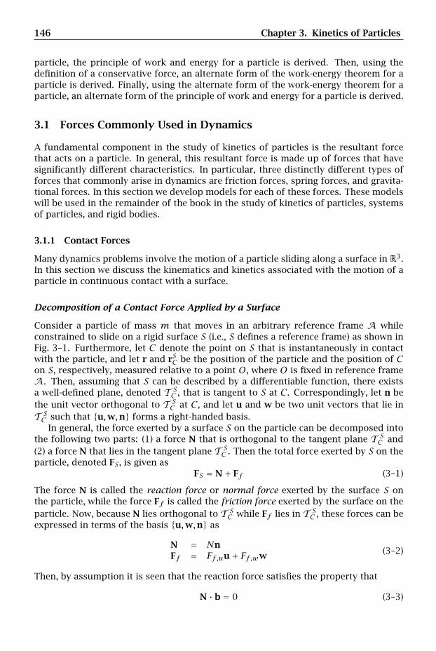
146 Chapter 3. Kinetics of Particles
particle, the principle of work and energy for a particle is derived. Then, using thedefinition of a conservative force, an alternate form of the work-energy theorem for aparticle is derived. Finally, using the alternate form of the work-energy theorem for aparticle, an alternate form of the principle of work and energy for a particle is derived.
3.1 Forces Commonly Used in Dynamics
A fundamental component in the study of kinetics of particles is the resultant forcethat acts on a particle. In general, this resultant force is made up of forces that havesignificantly different characteristics. In particular, three distinctly different types offorces that commonly arise in dynamics are friction forces, spring forces, and gravita-tional forces. In this section we develop models for each of these forces. These modelswill be used in the remainder of the book in the study of kinetics of particles, systemsof particles, and rigid bodies.
3.1.1 Contact Forces
Many dynamics problems involve the motion of a particle sliding along a surface in R3.In this section we discuss the kinematics and kinetics associated with the motion of aparticle in continuous contact with a surface.
Decomposition of a Contact Force Applied by a Surface
Consider a particle of mass m that moves in an arbitrary reference frame A whileconstrained to slide on a rigid surface S (i.e., S defines a reference frame) as shown inFig. 3–1. Furthermore, let C denote the point on S that is instantaneously in contactwith the particle, and let r and rSC be the position of the particle and the position of Con S, respectively, measured relative to a point O, where O is fixed in reference frameA. Then, assuming that S can be described by a differentiable function, there existsa well-defined plane, denoted T S
C , that is tangent to S at C . Correspondingly, let n bethe unit vector orthogonal to T S
C at C , and let u and w be two unit vectors that lie inT SC such that u,w,n forms a right-handed basis.
In general, the force exerted by a surface S on the particle can be decomposed intothe following two parts: (1) a force N that is orthogonal to the tangent plane T S
C and(2) a force N that lies in the tangent plane T S
C . Then the total force exerted by S on theparticle, denoted FS, is given as
FS = N+ Ff (3–1)
The force N is called the reaction force or normal force exerted by the surface S onthe particle, while the force Ff is called the friction force exerted by the surface on theparticle. Now, because N lies orthogonal to T S
C while Ff lies in T SC , these forces can be
expressed in terms of the basis u,w,n as
N = NnFf = Ff ,uu+ Ff ,ww (3–2)
Then, by assumption it is seen that the reaction force satisfies the property that
N · b = 0 (3–3)
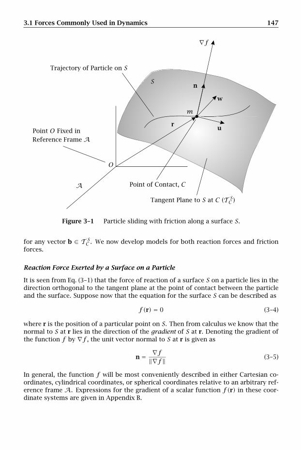
3.1 Forces Commonly Used in Dynamics 147
∇f
Trajectory of Particle on S
Tangent Plane to S at C (T SC )
Point O Fixed in
A
Reference Frame A
Point of Contact, C
n
ru
w
m
O
S
Figure 3–1 Particle sliding with friction along a surface S.
for any vector b ∈ T SC . We now develop models for both reaction forces and friction
forces.
Reaction Force Exerted by a Surface on a Particle
It is seen from Eq. (3–1) that the force of reaction of a surface S on a particle lies in thedirection orthogonal to the tangent plane at the point of contact between the particleand the surface. Suppose now that the equation for the surface S can be described as
f(r) = 0 (3–4)
where r is the position of a particular point on S. Then from calculus we know that thenormal to S at r lies in the direction of the gradient of S at r. Denoting the gradient ofthe function f by ∇f , the unit vector normal to S at r is given as
n = ∇f‖∇f‖ (3–5)
In general, the function f will be most conveniently described in either Cartesian co-ordinates, cylindrical coordinates, or spherical coordinates relative to an arbitrary ref-erence frame A. Expressions for the gradient of a scalar function f(r) in these coor-dinate systems are given in Appendix B.
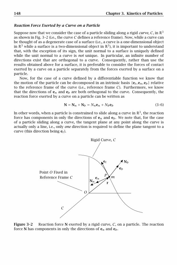
148 Chapter 3. Kinetics of Particles
Reaction Force Exerted by a Curve on a Particle
Suppose now that we consider the case of a particle sliding along a rigid curve, C, in R3
as shown in Fig. 3–2 (i.e., the curve C defines a reference frame). Now, while a curve canbe thought of as a degenerate case of a surface (i.e., a curve is a one-dimensional objectin R3 while a surface is a two-dimensional object in R3), it is important to understandthat, with the exception of its sign, the unit normal to a surface is uniquely definedwhile the unit normal to a curve is not unique. In particular, an infinite number ofdirections exist that are orthogonal to a curve. Consequently, rather than use theresults obtained above for a surface, it is preferable to consider the forces of contactexerted by a curve on a particle separately from the forces exerted by a surface on aparticle.
Now, for the case of a curve defined by a differentiable function we know thatthe motion of the particle can be decomposed in an intrinsic basis et,en,eb relativeto the reference frame of the curve (i.e., reference frame C). Furthermore, we knowthat the directions of en and eb are both orthogonal to the curve. Consequently, thereaction force exerted by a curve on a particle can be written as
N = Nn +Nb = Nnen +Nbeb (3–6)
In other words, when a particle is constrained to slide along a curve in R3, the reactionforce has components in only the directions of en and eb. We note that, for the caseof a particle sliding along a curve, the tangent plane at any point along the curve isactually only a line, i.e., only one direction is required to define the plane tangent to acurve (this direction being et).
Rigid Curve, C
Point O Fixed inReference Frame C
Nn
Nbet
en
eb
r
m
O
P
C
Figure 3–2 Reaction force N exerted by a rigid curve, C, on a particle. The reactionforce N has components in only the directions of en and eb.

3.1 Forces Commonly Used in Dynamics 149
Friction Force Exerted by a Surface on a Particle
With regard to the force of friction exerted by a surface on a particle, the two mostcommon types of friction forces are Coulomb friction (Coulomb, 1785) and viscousfriction. We now derive models for a Coulomb friction force and a viscous frictionforce.
Coulomb Friction
The fundamental assumption in Coulomb friction is that the friction force Ff is pro-portional to the normal force. Furthermore, the constant of proportionality is calledthe coefficient of Coulomb friction.1 There are two types of Coulomb friction: staticand dynamic. Static Coulomb friction arises when the relative velocity between theparticle and the instantaneous point of contact of the particle with the surface is zero,i.e., vrel = 0. For the case of static Coulomb friction we have
‖Ff‖ ≤ µs‖N‖ (3–7)
where the constant µs is called the coefficient of static Coulomb friction. ExaminingEq. (3–7), it is seen that, in the case of static Coulomb friction, the actual frictionforce is indeterminate because the magnitude of Ff is only known to be less than theproduct of the coefficient of static friction and the normal force. Dynamic Coulombfriction arises when vrel ≠ 0. For the case of dynamic Coulomb friction we have
Ff = −µd‖N‖vrel
‖vrel‖(3–8)
where the constant µd is called the coefficient of dynamic Coulomb friction and vrel isthe velocity of the particle relative to the point on S that is instantaneously in contactwith the particle (see Section 2.14 for the definition of vrel). It is noted that the dynamicCoulomb friction force is obtained using the relative velocity between the particle andthe surface, not the velocity of the particle.
Viscous Friction
The fundamental assumption in viscous friction is that the friction force is propor-tional to vrel and has a constant of proportionality c called the coefficient of viscousfriction. The viscous friction force is then given as
Ff = −cvrel (3–9)
As with dynamic Coulomb friction, it is noted that the viscous friction force is obtainedusing the relative velocity between the particle and the surface, not the velocity of theparticle (again, see Section 2.14 for the definition of vrel).
1Models for Coulomb friction can be found in many books on dynamics. See Beer and Johnston (1997),Bedford and Fowler (2005), or Greenwood (1988) for other descriptions of Coulomb friction.
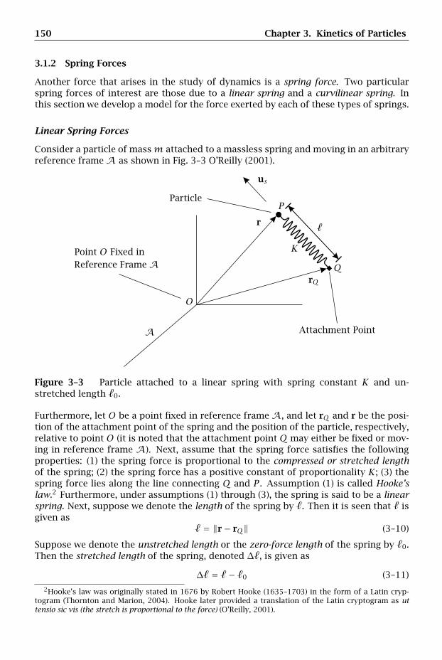
150 Chapter 3. Kinetics of Particles
3.1.2 Spring Forces
Another force that arises in the study of dynamics is a spring force. Two particularspring forces of interest are those due to a linear spring and a curvilinear spring. Inthis section we develop a model for the force exerted by each of these types of springs.
Linear Spring Forces
Consider a particle of massm attached to a massless spring and moving in an arbitraryreference frame A as shown in Fig. 3–3 O’Reilly (2001).
Point O Fixed in
A Attachment Point
Reference Frame A
Particle
r
rQ
us
K
O
P
Q
Figure 3–3 Particle attached to a linear spring with spring constant K and un-stretched length 0.
Furthermore, let O be a point fixed in reference frame A, and let rQ and r be the posi-tion of the attachment point of the spring and the position of the particle, respectively,relative to point O (it is noted that the attachment point Q may either be fixed or mov-ing in reference frame A). Next, assume that the spring force satisfies the followingproperties: (1) the spring force is proportional to the compressed or stretched lengthof the spring; (2) the spring force has a positive constant of proportionality K; (3) thespring force lies along the line connecting Q and P . Assumption (1) is called Hooke’slaw.2 Furthermore, under assumptions (1) through (3), the spring is said to be a linearspring. Next, suppose we denote the length of the spring by . Then it is seen that isgiven as
= ‖r− rQ‖ (3–10)
Suppose we denote the unstretched length or the zero-force length of the spring by 0.Then the stretched length of the spring, denoted ∆, is given as
∆ = − 0 (3–11)
2Hooke’s law was originally stated in 1676 by Robert Hooke (1635–1703) in the form of a Latin cryp-togram (Thornton and Marion, 2004). Hooke later provided a translation of the Latin cryptogram as uttensio sic vis (the stretch is proportional to the force) (O’Reilly, 2001).

3.1 Forces Commonly Used in Dynamics 151
Applying assumptions (1) and (2), the magnitude of the force generated by the spring,denoted ‖Fs‖, is given as
‖Fs‖ = K∣∣( − 0)
∣∣ (3–12)
Also, applying assumption (3) and denoting the unit vector from rQ to r as us , thedirection of the spring force is given as
us =r− rQ‖r− rQ‖
(3–13)
It can be seen from Eq. (3–11) that the quantity −0 can be either positive or negative.Therefore, we need to examine two cases.
Case 1: − 0 < 0 (Compression)
In the case where − 0 < 0, the spring is said to be compressed. In the case ofcompression, the spring exerts a force on the particle in the direction from rQ to r,i.e., the spring force is in the direction of us . However, because − 0 < 0 when thespring is compressed, we have
∣∣ − 0∣∣ = −( − 0) (3–14)
The force of the spring in compression is then given as
Fs = −K( − 0)us (3–15)
Case 2: − 0 > 0 (Extension)
In the case where − 0 > 0, the spring is said to be extended or stretched. In the caseof extension, the spring exerts a force on the particle in the direction r to rQ, i.e., thespring force is in the direction of −us . However, because − 0 > 0 when the spring iscompressed, we have ∣∣ − 0
∣∣ = ( − 0) (3–16)
The force of the spring in extension is then given as
Fs = K( − 0) [−us] (3–17)
Equation (3–17) can be rewritten as
Fs = −K( − 0)us (3–18)
The results of the two cases show that, regardless of whether the spring is compressedor extended, the force exerted by the spring on the particle is given as
Fs = −K( − 0)us (3–19)
where is the length of the spring and is obtained from Eq. (3–10), 0 is the unstretchedlength of the spring, and us is obtained from Eq. (3–13).
It is important to note that the aforementioned model for spring force is an ap-proximation based on experimental evidence. Consequently, Hooke’s law is not alwaysvalid. For example, it is clear that a real spring cannot be stretched to an arbitrarily

152 Chapter 3. Kinetics of Particles
large length (since the spring would break or permanently deform so that it would notreturn to its original shape) nor can a real spring be compressed to a length of zero(since the spring has mass and, thus, occupies a nonzero amount of space). Neverthe-less, for many engineering applications where the spring stretches or compresses to a“reasonable” length, the model for a linear spring obtained in Eq. (3–19) is an excellentapproximation.
Curvilinear Spring
Consider a particle attached to a massless spring and moving in an arbitrary referenceframe A such that the particle slides along a rigid curve C (i.e., C defines a referenceframe) and the spring conforms to the shape of C as shown in Fig. 3–4. Furthermore,suppose that one end of the spring is located at a point Q on C while the other endof the spring is attached to the particle (it is noted that point Q may either be fixed ormoving relative to C). Finally, let the force generated by the spring have the form
Fs = −K( − 0)et (3–20)
where K is the spring constant, is the stretched length of the spring along the curveC, 0 is the unstretched length of the spring, and et is the tangent vector at point P asviewed by an observer fixed to C. A spring whose force satisfies Eq. (3–20) is called acurvilinear spring; a schematic of a curvilinear spring is shown in Fig. 3–4.
Point O Fixed in
A
Reference Frame Aet
r
rQ
m
K
O
P
Q
C
Figure 3–4 Particle sliding on a curve C while attached to a curvilinear spring withspring constant K and unstretched length 0.
As with a linear spring, in the case of either compression or extension, the force gen-erated by a curvilinear spring satisfies Eq. (3–20). Moreover, it is seen from Eq. (3–20)that a curvilinear spring is a generalization of a linear spring to the case where thespring bends to conform to the shape of an arbitrary curve.
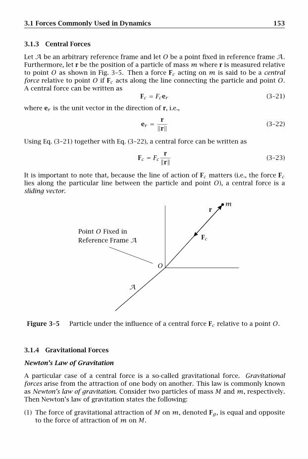
3.1 Forces Commonly Used in Dynamics 153
3.1.3 Central Forces
Let A be an arbitrary reference frame and let O be a point fixed in reference frame A.Furthermore, let r be the position of a particle of massm where r is measured relativeto point O as shown in Fig. 3–5. Then a force Fc acting on m is said to be a centralforce relative to point O if Fc acts along the line connecting the particle and point O.A central force can be written as
Fc = Fcer (3–21)
where er is the unit vector in the direction of r, i.e.,
er = r‖r‖ (3–22)
Using Eq. (3–21) together with Eq. (3–22), a central force can be written as
Fc = Fc r‖r‖ (3–23)
It is important to note that, because the line of action of Fc matters (i.e., the force Fclies along the particular line between the particle and point O), a central force is asliding vector.
Point O Fixed in
A
Reference Frame A Fc
rm
O
Figure 3–5 Particle under the influence of a central force Fc relative to a point O.
3.1.4 Gravitational Forces
Newton’s Law of Gravitation
A particular case of a central force is a so-called gravitational force. Gravitationalforces arise from the attraction of one body on another. This law is commonly knownas Newton’s law of gravitation. Consider two particles of mass M and m, respectively.Then Newton’s law of gravitation states the following:
(1) The force of gravitational attraction of M on m, denoted Fg , is equal and oppositeto the force of attraction of m on M .
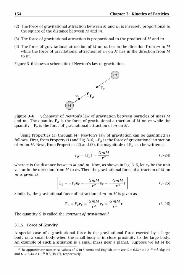
154 Chapter 3. Kinetics of Particles
(2) The force of gravitational attraction between M and m is inversely proportional tothe square of the distance between M and m.
(3) The force of gravitational attraction is proportional to the product of M and m.
(4) The force of gravitational attraction of M on m lies in the direction from m to Mwhile the force of gravitational attraction of m on M lies in the direction from Mto m.
Figure 3–6 shows a schematic of Newton’s law of gravitation.
er −Fg
Fg
m
M
Figure 3–6 Schematic of Newton’s law of gravitation between particles of mass Mand m. The quantity Fg is the force of gravitational attraction of M on m while thequantity −Fg is the force of gravitational attraction of m on M .
Using Properties (1) through (4), Newton’s law of gravitation can be quantified asfollows. First, from Property (1) and Fig. 3–6, −Fg is the force of gravitational attractionof m on M . Next, from Properties (2) and (3), the magnitude of Fg can be written as
Fg = ‖Fg‖ = GmMr 2(3–24)
where r is the distance between M andm. Now, as shown in Fig. 3–6, let er be the unitvector in the direction from M tom. Then the gravitational force of attraction of M onm is given as
Fg = −Fger = −GmMr 2er = −GmMr 3
r (3–25)
Similarly, the gravitational force of attraction of m on M is given as
−Fg = Fger = GmMr 2er = GmMr 3
r (3–26)
The quantity G is called the constant of gravitation.3
3.1.5 Force of Gravity
A special case of a gravitational force is the gravitational force exerted by a largebody on a small body when the small body is in close proximity to the large body.An example of such a situation is a small mass near a planet. Suppose we let M be
3The approximate numerical values of G in SI units and English units are G = 6.673×10⁻¹¹m3/(kg s2)and G = 3.44× 10⁻⁸ ft4/(lb s4), respectively.
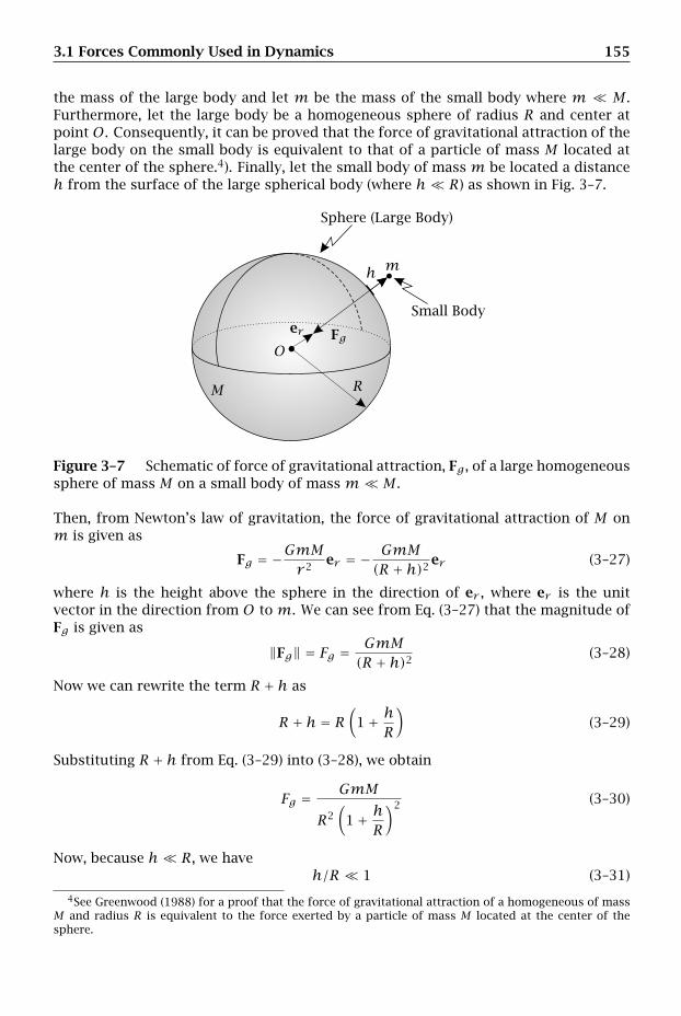
3.1 Forces Commonly Used in Dynamics 155
the mass of the large body and let m be the mass of the small body where m M .Furthermore, let the large body be a homogeneous sphere of radius R and center atpoint O. Consequently, it can be proved that the force of gravitational attraction of thelarge body on the small body is equivalent to that of a particle of mass M located atthe center of the sphere.4). Finally, let the small body of mass m be located a distanceh from the surface of the large spherical body (where h R) as shown in Fig. 3–7.
Sphere (Large Body)
Small Bodyer Fg
mh
M
O
R
Figure 3–7 Schematic of force of gravitational attraction, Fg , of a large homogeneoussphere of mass M on a small body of mass m M .
Then, from Newton’s law of gravitation, the force of gravitational attraction of M onm is given as
Fg = −GmMr 2er = − GmM
(R + h)2 er (3–27)
where h is the height above the sphere in the direction of er , where er is the unitvector in the direction from O tom. We can see from Eq. (3–27) that the magnitude ofFg is given as
‖Fg‖ = Fg = GmM(R + h)2 (3–28)
Now we can rewrite the term R + h as
R + h = R(
1+ hR
)(3–29)
Substituting R + h from Eq. (3–29) into (3–28), we obtain
Fg = GmM
R2(
1+ hR
)2 (3–30)
Now, because h R, we haveh/R 1 (3–31)
4See Greenwood (1988) for a proof that the force of gravitational attraction of a homogeneous of massM and radius R is equivalent to the force exerted by a particle of mass M located at the center of thesphere.
156 Chapter 3. Kinetics of Particles
Consequently, (1+ h
R
)2
≈ 1 (3–32)
which implies that
Fg ≈ GmMR2=mGM
R2(3–33)
Then, for small values of h, the force of gravitational attraction of M on m is given as
Fg ≈ −mGMR2er (3–34)
The quantity−GM/R2er (3–35)
is often called the local acceleration due to gravity. For convenience, we write
g = −GMR2
er = −ger (3–36)
where g = GM/R2. It is also noted that when using the approximation of Eq. (3–36),the direction er is assumed to be a constant and is often denoted ev . The force ofgravitation in Eq. (3–34) can then be written as
Fg = −mgev (3–37)
For convenience, the direction ev is called the local vertical direction or simply thevertical direction. Furthermore, the acceleration due to gravity, denoted g, is given as
g = −gev (3–38)
Then the force of gravity can be written as
Fg =mg (3–39)
It is noted that for some problems the direction of Fg in Eq. (3–39) may be more conve-niently specified using the direction opposite the local vertical, in which case the forceof gravity is given as
Fg =mguv (3–40)
where uv = −ev .
3.2 Inertial Reference Frames
Before proceeding to describe Newton’s laws, it is important to emphasize that, whilemotion can be observed in an arbitrary (noninertial) reference frame, the laws of mo-tion for a particle are valid only in an inertial reference frame. Therefore, from thispoint forth, with only a few exceptions, all kinematic quantities will be defined rela-tive to an inertial reference frame. For clarity, in the development of the theory, theleft superscript N will always denote motion as viewed by an observer in an inertialreference frame. Finally, when solving problems, the left superscript F will denote afixed inertial reference frame while any other calligraphic letter (e.g., A, B) will denotea general (noninertial) reference frame.

3.3 Newton’s Laws for a Particle 157
3.3 Newton’s Laws for a Particle
We now state the axioms that govern the motion of particles. These axioms are calledNewton’s laws and are given as follows:
Newton’s 1st Law:
An object in motion tends to remain in motion unless acted upon by an external force.An object at rest tends to remain at rest unless acted upon by an outside force.
Newton’s 2nd Law:5
Let F be the total or resultant force acting on a particle of mass m. Then
F =mNa (3–41)
where Na ≡ a is the acceleration of the particle as viewed by an observer in any inertialreference frame N (Newton, 1687).6
Newton’s 3rd Law:
For every action, there is an equal and opposite reaction.
3.4 Comments on Newton’s Laws
It can be seen that the statements of Newton’s laws are extremely simple. However,it is important for the reader to understand that the application of Newton’s laws isoften a highly nontrivial matter. First, because Newton’s laws are valid only in aninertial reference frame, it is necessary to determine the acceleration of the particle inan inertial reference frame using observations of the motion in a noninertial referenceframe. Next, once an observation reference frame has been chosen, it is necessary tospecify an appropriate coordinate system in which to quantify the motion. While inprinciple any coordinate system may be used, choosing an inappropriate coordinatesystem can result in extremely tedious algebra and can distort the key aspects of aparticular problem. Consequently, it is extremely important to think carefully and tochoose a coordinate system that is well suited to the geometry of the problem beingsolved. The acceleration of the particle in an inertial reference frame must then becomputed in terms of the chosen coordinate system. Finally, the forces acting on theparticle must be resolved in the chosen coordinate system. While it may seem obvious,it is not only necessary to take great care to ensure that each force is specified in theproper direction, but it is also necessary to examine carefully the problem to ensurethat no forces are omitted.
5Newton’s 2nd law is an example of Galilean invariance or Newtonian relativity.6Isaac Newton (1642–1727) wrote his 2nd law in Volume 1 of his famous Philosophiae Naturalis Principia
Mathematica (better known as Principia). Newton’s Principia was originally published in 1687. An Englishtranslation of Principia is given in Newton (1687).
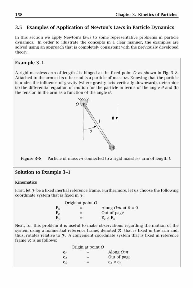
158 Chapter 3. Kinetics of Particles
3.5 Examples of Application of Newton’s Laws in Particle Dynamics
In this section we apply Newton’s laws to some representative problems in particledynamics. In order to illustrate the concepts in a clear manner, the examples aresolved using an approach that is completely consistent with the previously developedtheory.
Example 3–1
A rigid massless arm of length l is hinged at the fixed point O as shown in Fig. 3–8.Attached to the arm at its other end is a particle of massm. Knowing that the particleis under the influence of gravity (where gravity acts vertically downward), determine(a) the differential equation of motion for the particle in terms of the angle θ and (b)the tension in the arm as a function of the angle θ.
gl
m
O
θ
Figure 3–8 Particle of mass m connected to a rigid massless arm of length l.
Solution to Example 3–1
Kinematics
First, let F be a fixed inertial reference frame. Furthermore, let us choose the followingcoordinate system that is fixed in F :
Origin at point OEx = Along Om at θ = 0Ez = Out of pageEy = Ez × Ex
Next, for this problem it is useful to make observations regarding the motion of thesystem using a noninertial reference frame, denoted R, that is fixed in the arm and,thus, rotates relative to F . A convenient coordinate system that is fixed in referenceframe R is as follows:
Origin at point Oer = Along Omez = Out of pageeθ = ez × er
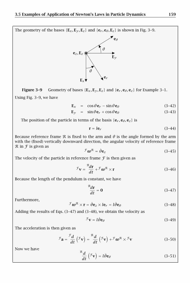
3.5 Examples of Application of Newton’s Laws in Particle Dynamics 159
The geometry of the bases Ex,Ey,Ez and er ,eθ,Ez is shown in Fig. 3–9.
er
eθ
Ex
Eyez,Ez
θ
θ
Figure 3–9 Geometry of bases Ex,Ey,Ez and er ,eθ,ez for Example 3–1.
Using Fig. 3–9, we have
Ex = cosθer − sinθeθ (3–42)
Ey = sinθer + cosθeθ (3–43)
The position of the particle in terms of the basis er ,eθ,ez is
r = ler (3–44)
Because reference frame R is fixed to the arm and θ is the angle formed by the armwith the (fixed) vertically downward direction, the angular velocity of reference frameR in F is given as
FωR = θez (3–45)
The velocity of the particle in reference frame F is then given as
Fv =Rdrdt+FωR × r (3–46)
Because the length of the pendulum is constant, we have
Rdrdt
= 0 (3–47)
Furthermore,FωR × r = θez × ler = lθeθ (3–48)
Adding the results of Eqs. (3–47) and (3–48), we obtain the velocity as
Fv = lθeθ (3–49)
The acceleration is then given as
Fa =Fddt
(Fv)=Rddt
(Fv)+FωR × Fv (3–50)
Now we haveRddt
(Fv)= lθeθ (3–51)

160 Chapter 3. Kinetics of Particles
andFωR × Fv = θez × lθeθ = −lθ2er (3–52)
The acceleration of the particle is then given as
Fa = −lθ2er + lθeθ (3–53)
Kinetics
The free body diagram of the particle is shown in Fig. 3–10.
Rmg
Figure 3–10 Free body diagram of particle for Example 3–1.
Using Fig. 3–10, it can be seen that the following two forces act on the particle:
mg = Force of gravityR = Reaction force exerted by arm on particle
Now, because the force of gravity acts vertically downward, we have
mg =mgEx (3–54)
Then, substituting the result of Eq. (3–42) into (3–54), the force of gravity is obtainedas
mg =mg cosθer −mg sinθeθ (3–55)
Next, the reaction force of the arm on the particle, R, must lie in along the arm, i.e., Rmust lie in the er -direction. However, because it is not known at this point whether Rlies in the positive or negative er -direction, the sign of the reaction force is not known.Therefore, we must specify R as
R = Rer (3–56)
where the scalar R must be determined. Using the expressions for mg from Eq. (3–55)and R from Eq. (3–56), the resultant force acting on the particle can be written as
F =mg+ R =mg cosθer −mg sinθeθ + Rer (3–57)
Combining er and eθ components, Eq. (3–57) can be rewritten as
F = (mg cosθ + R)er −mg sinθeθ (3–58)
Then, applying Newton’s 2nd, we have
F =mNa (3–59)

3.5 Examples of Application of Newton’s Laws in Particle Dynamics 161
where N is any inertial reference frame. Noting that F is an inertial reference frame,we can substitute F from Eq. (3–58) and Fa from Eq. (3–53) to give
(mg cosθ + R)er −mg sinθeθ =m(−lθ2er + lθeθ) = −mlθ2er +mlθeθ (3–60)
Equating the er and eθ components, we obtain the following two scalar equations:
mg cosθ + R = −mlθ2 (3–61)
−mg sinθ = mlθ (3–62)
(a) Differential Equation of Motion in Terms of θ
In this example there is only one variable used to describe the motion, namely the angleθ. Consequently, only one differential equation is required to describe the motion. Inorder to obtain the differential equation, we need to determine an expression that is afunction of θ and time derivatives of θ along with any constants given in the problem.It is noted that the differential equation cannot contain any reaction forces because thereaction forces are unknown. In this example, the differential equation arises directlyfrom the equations that result from the application of Newton’s 2nd law. In particular,Eq. (3–62) is the differential equation of motion. Consequently, we have
mlθ = −mg sinθ (3–63)
Rearranging Eq. (3–63) and dropping m from both sides, we obtain
θ = −gl
sinθ (3–64)
(b) Tension in Arm as a Function of Angle θ
Solving Eq. (3–61) for R, we obtain
R = −mg cosθ −mlθ2 (3–65)
It can be seen from Eq. (3–56) that R is a function of θ2. Consequently, in order toobtain an expression for the tension in the arm as a function of the angle θ, it isnecessary to obtain an expression for θ2 in terms of θ. An expression for θ2 in termsof θ can be obtained from Eq. (3–64). In particular, we see from Eq. (3–64) that themotion is a function of the single variable θ. Consequently, the results of rectilinearmotion from Section 2.7 can be applied. In this case, the angular acceleration θ is afunction of the angular position θ. Hence we are in Case 3 as described in Section 2.7on page 41. First, we can apply Eq. (2–57) by making the following substitutions:
x → θv → θa → θ
We then have
θ = ddt(θ) = dθ
dθdθdt
= θ dθdθ
(3–66)
162 Chapter 3. Kinetics of Particles
Next, substituting the expression for θ into Eq. (3–64), we obtain
θdθdθ
= −gl
sinθ (3–67)
Using the method of separation of variables (Kreyszig, 1988), we have
θdθ = −gl
sinθdθ (3–68)
Then, integrating both sides of Eq. (3–68) gives
∫ θθ0
νdν =∫ θθ0
−gl
sinηdη (3–69)
where ν and η are dummy variables of integration. Computing the integrals on bothsides of Eq. (3–69), we obtain
ν2
2
∣∣∣∣∣θ
θ0
= gl
cosη∣∣∣∣θθ0
(3–70)
Simplifying Eq. (3–70), we obtain
θ2 − θ20 =
2gl(cosθ − cosθ 0) (3–71)
Therefore,
θ2 = θ20 +
2gl(cosθ − cosθ 0) (3–72)
Then, substituting the expression for θ2 from Eq. (3–72) into (3–65), we obtain
R = −mg cosθ −ml[θ2
0 +2gl(cosθ − cosθ 0)
](3–73)
Simplifying Eq. (3–73), we obtain
R = −3mg cosθ −mlθ20 + 2mg cosθ 0 (3–74)
The reaction force as a function of θ is then given as
R = Rer =[−3mg cosθ −mlθ2
0 + 2mg cosθ 0
]er (3–75)
Comments on Solution Approach and Results Obtained
The current example demonstrates several important components that are commonto all engineering dynamics problems. The first important component is kinematics.In Chapter 2 we studied methods to derive velocity and acceleration in various co-ordinate systems. The current example demonstrates the importance of choosing anappropriate coordinate system in which to solve the problem. Had a coordinate systemdifferent from cylindrical coordinates been chosen (e.g., a fixed Cartesian coordinatesystem), the equations resulting from the application of Newton’s 2nd law would havebeen more complicated. Second, the choice of cylindrical coordinates made it easier to

3.5 Examples of Application of Newton’s Laws in Particle Dynamics 163
understand the motion. In particular, the motion is naturally decoupled into radial andtransverse motion using cylindrical coordinates. Therefore, had a different coordinatesystem been chosen, the equations resulting from Newton’s 2nd law would have beenmore difficult to interpret.
The second important component is the application of Newton’s 2nd law. In thisexample we had two forces acting on the particle. The first force, namely that of grav-ity, was known. Consequently, it was necessary to properly specify both its magnitudeand direction. In particular, for this example gravity acted vertically downward. There-fore, it was necessary to ensure that the force of gravity was placed in the positive Ex-direction. The second force, namely that of the reaction force of the arm, was unknownin the sense that its sign was not known. Therefore, it was not important whether thisforce was initially chosen to be in the er -direction or in the negative er -direction; theproper sign of R was determined from the algebra.
The third important component was the ability to apply engineering mathematics.In this example we were asked specifically to determine the tension in the arm as afunction of the angle θ. Once the kinematics and kinetics were completed, the originaldynamics problem was turned into a math problem. In order to solve this math prob-lem, it was necessary to recall fundamental concepts from algebra and calculus. While,strictly speaking, dynamics is not mathematics, it is virtually impossible to solve anydynamics problem without sufficient knowledge of mathematics. Consequently, thereader should keep in mind the importance of mathematics in the formulation andsolution of any dynamics problem.
Example 3–2
A particle of mass m slides without friction along a fixed track in the form of aparabola as shown in Fig. 3–11. The equation for the parabola is
y = r2
2R(3–76)
where R is a constant, r is the distance from point O to point Q, point Q is theprojection of point P onto the horizontal direction, and y is the vertical distance.Knowing that gravity acts downward and that the initial conditions are r(t = 0) = r0
and r (t = 0) = 0, determine (a) the differential equation of motion for the particle interms of the variable r , and (b) an expression for r 2 as a function of r .
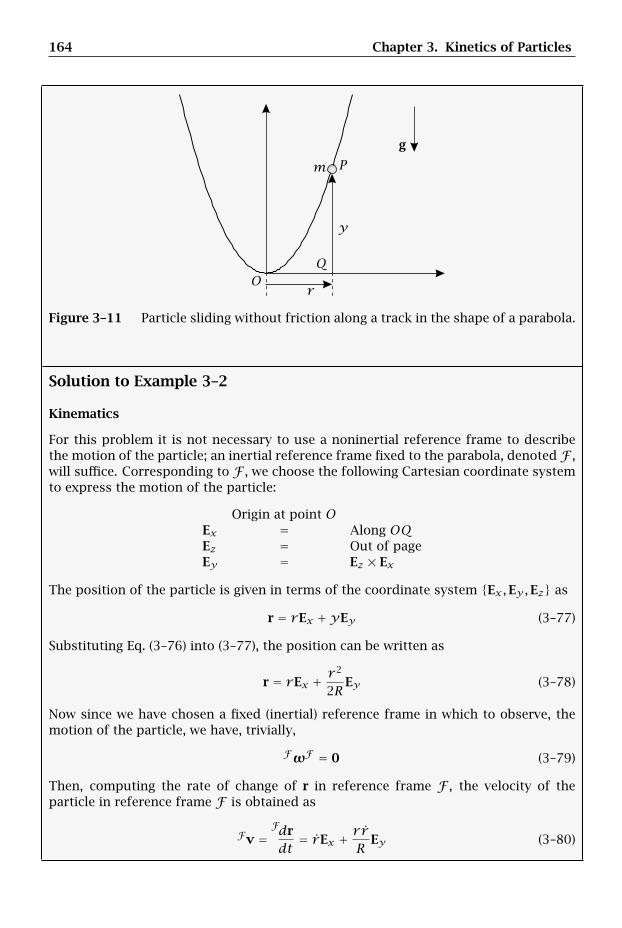
164 Chapter 3. Kinetics of Particles
g
m
r
y
O
P
Q
Figure 3–11 Particle sliding without friction along a track in the shape of a parabola.
Solution to Example 3–2
Kinematics
For this problem it is not necessary to use a noninertial reference frame to describethe motion of the particle; an inertial reference frame fixed to the parabola, denoted F ,will suffice. Corresponding to F , we choose the following Cartesian coordinate systemto express the motion of the particle:
Origin at point OEx = Along OQEz = Out of pageEy = Ez × Ex
The position of the particle is given in terms of the coordinate system Ex,Ey,Ez as
r = rEx +yEy (3–77)
Substituting Eq. (3–76) into (3–77), the position can be written as
r = rEx + r2
2REy (3–78)
Now since we have chosen a fixed (inertial) reference frame in which to observe, themotion of the particle, we have, trivially,
FωF = 0 (3–79)
Then, computing the rate of change of r in reference frame F , the velocity of theparticle in reference frame F is obtained as
Fv =Fdrdt
= rEx + r rR Ey (3–80)
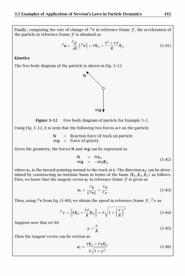
3.5 Examples of Application of Newton’s Laws in Particle Dynamics 165
Finally, computing the rate of change of Fv in reference frame F , the acceleration ofthe particle in reference frame F is obtained as
Fa =Fddt
(Fv)= rEx + r
2 + r rR
Ey (3–81)
Kinetics
The free body diagram of the particle is shown in Fig. 3–12.
N
mg
Figure 3–12 Free body diagram of particle for Example 3–2.
Using Fig. 3–12, it is seen that the following two forces act on the particle:
N = Reaction force of track on particlemg = Force of gravity
Given the geometry, the forces N and mg can be expressed as
N = Nenmg = −mgEy
(3–82)
where en is the inward pointing normal to the track at r. The direction en can be deter-mined by constructing an intrinsic basis in terms of the basis Ex,Ey,Ez as follows.First, we know that the tangent vector et in reference frame F is given as
et =Fv‖Fv‖ =
FvFv
(3–83)
Then, using Fv from Eq. (3–80), we obtain the speed in reference frame F , Fv as
Fv =∥∥∥∥rEx + r rR Ey
∥∥∥∥ = r√
1+(rR
)2
(3–84)
Suppose now that we let
γ = rR
(3–85)
Then the tangent vector can be written as
et =rEx + rγEy
r√
1+ γ2(3–86)
166 Chapter 3. Kinetics of Particles
Equation (3–86) simplifies to
et =Ex + γEy√
1+ γ2(3–87)
Next, because the motion is two-dimensional, the principal unit bi-normal vector, eb,must lie in the direction orthogonal to the plane of motion. Consequently, we have
eb = Ez (3–88)
The unit normal vector, en, is then given as
en = eb × et (3–89)
Therefore,
en = Ez ×Ex + γEy√
1+ γ2(3–90)
Taking the vector products in Eq. (3–90), we obtain
en =Ey − γEx√
1+ γ2(3–91)
Rearranging Eq. (3–91), we have
en =−γEx + Ey√
1+ γ2(3–92)
Then the reaction force N is given as
N = Nen = N⎡⎣−γEx + Ey√
1+ γ2
⎤⎦ (3–93)
The resultant force, F, on the particle is then given as
F = N+mg = N⎡⎣−γEx + Ey√
1+ γ2
⎤⎦−mgEy (3–94)
Rearranging Eq. (3–94), we have
F = −N γ√1+ γ2
Ex +⎡⎣ N√
1+ γ2−mg
⎤⎦Ey (3–95)
Then, applying Newton’s 2nd law by setting F equal to mFa using Fa from Eq. (3–81),we obtain
−N γ√1+ γ2
Ex +⎡⎣ N√
1+ γ2−mg
⎤⎦Ey =mrEx +mr
2 + r rR
Ey (3–96)
Equating components yields the following two scalar equations:
−N γ√1+ γ2
= mr
N√1+ γ2
−mg = mr 2 + r rR
(3–97)

3.5 Examples of Application of Newton’s Laws in Particle Dynamics 167
(a) Differential Equation of Motion in Terms of r
Equation (3–97) can be rewritten as
−N γ√1+ γ2
= mr
N√1+ γ2
= mg +mr2 + r rR
(3–98)
Dividing the two expressions in Eq. (3–98), we obtain
−γ = mr
mg +mr2 + r rR
(3–99)
Simplifying Eq. (3–99) by dropping m, we obtain
−γ = r
g + r2 + r rR
(3–100)
Recalling from Eq. (3–85) that γ = r/R, Eq. (3–100) can be written as
− rR= r
g + r2 + r rR
(3–101)
Rearranging Eq. (3–101), we obtain
−r[g + r
2 + r rR
]= Rr (3–102)
We then obtain
−rg − r r2 + r 2rR
= Rr (3–103)
Multiplying Eq. (3–103) by R, we obtain
−Rrg − r r 2 − r 2r = R2r (3–104)
Rearranging Eq. (3–104), we obtain the differential equation as
(r 2 + R2)r + r(r 2 + Rg) = 0 (3–105)
(b) Expression for r 2 as a Function of r
We start with the result from part (c), i.e., we start with Eq. (3–105). We know that
r = drdt
= drdrdrdt
= r drdr
(3–106)
The expression for r from Eq. (3–106) can then be substituted into Eq. (3–105). Thisgives
(r 2 + R2)rdrdr
+ r(r 2 + Rg) = 0 (3–107)
168 Chapter 3. Kinetics of Particles
Rearranging Eq. (3–107), we obtain
(r 2 + R2)rdrdr
= −r(r 2 + Rg) (3–108)
Separating r and r in Eq. (3–108), we have
rr 2 + Rgdr = −
rr 2 + R2
dr (3–109)
Integrating both sides, we obtain∫ rr0
νν2 + Rgdν =
∫ rr0
− ηη2 + R2
dη (3–110)
where ν and η are dummy variables of integration. Then, from Appendix B, we have∫ν
ν2 + a2dν = 1
2 ln |ν2 + a2| + C (3–111)
Applying the result of Eq. (3–111) in (3–110), we obtain
12
[ln |ν2 + Rg|
]rr0= −1
2
[ln |η2 + R2|
]rr0
(3–112)
Equation (3–112) simplifies to[ln |r 2 + Rg|
]rr0= −
[ln |r 2 + R2|
]rr0
(3–113)
We then obtain
ln |r 2 + Rg| − ln |r 20 + Rg| = ln |r 2
0 + R2| − ln |r 2 + R2| (3–114)
Simplifying Eq. (3–114), we have
ln
∣∣∣∣∣ r2 + Rgr 2
0 + Rg
∣∣∣∣∣ = ln
∣∣∣∣∣r20 + R2
r 2 + R2
∣∣∣∣∣ (3–115)
Taking exponentials on both sides of Eq. (3–115), we obtain
r 2 + Rgr 2
0 + Rg= r
20 + R2
r 2 + R2(3–116)
Rearranging Eq. (3–116), we obtain
r 2 = −Rg + (r 20 + Rg)
r 20 + R2
r 2 + R2(3–117)
Using the given initial condition r (t = 0) = 0, we obtain
r 2 = −Rg + Rgr20 + R2
r 2 + R2(3–118)
This last expression simplifies to
r 2 = r20 − r 2
r 2 + R2Rg (3–119)
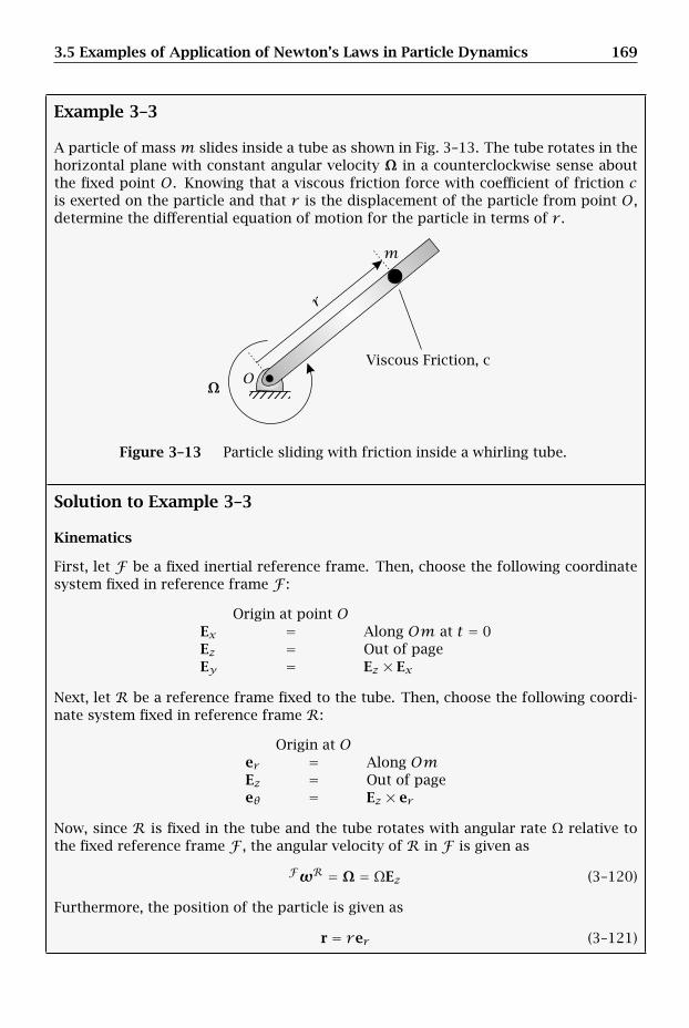
3.5 Examples of Application of Newton’s Laws in Particle Dynamics 169
Example 3–3
A particle of massm slides inside a tube as shown in Fig. 3–13. The tube rotates in thehorizontal plane with constant angular velocity Ω in a counterclockwise sense aboutthe fixed point O. Knowing that a viscous friction force with coefficient of friction cis exerted on the particle and that r is the displacement of the particle from point O,determine the differential equation of motion for the particle in terms of r .
Viscous Friction, c
m
r
OΩ
Figure 3–13 Particle sliding with friction inside a whirling tube.
Solution to Example 3–3
Kinematics
First, let F be a fixed inertial reference frame. Then, choose the following coordinatesystem fixed in reference frame F :
Origin at point OEx = Along Om at t = 0Ez = Out of pageEy = Ez × Ex
Next, let R be a reference frame fixed to the tube. Then, choose the following coordi-nate system fixed in reference frame R:
Origin at Oer = Along OmEz = Out of pageeθ = Ez × er
Now, since R is fixed in the tube and the tube rotates with angular rate Ω relative tothe fixed reference frame F , the angular velocity of R in F is given as
FωR = Ω = ΩEz (3–120)
Furthermore, the position of the particle is given as
r = rer (3–121)
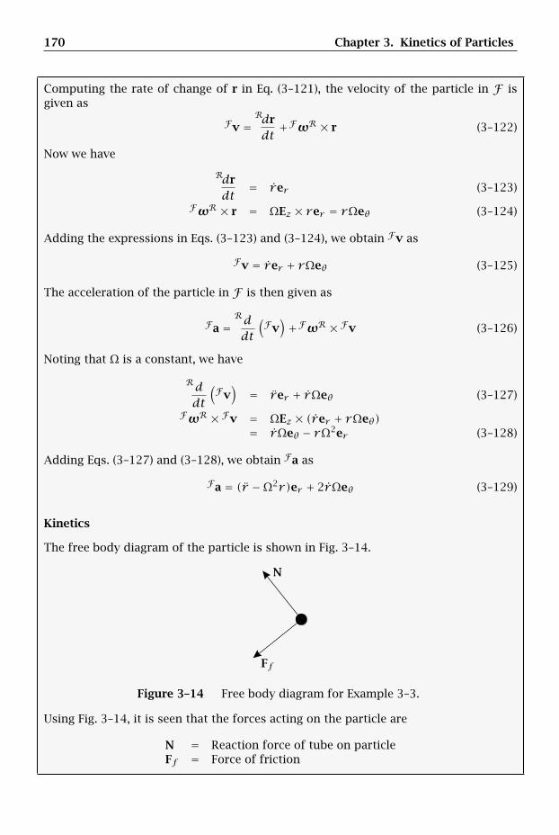
170 Chapter 3. Kinetics of Particles
Computing the rate of change of r in Eq. (3–121), the velocity of the particle in F isgiven as
Fv =Rdrdt+FωR × r (3–122)
Now we have
Rdrdt
= rer (3–123)
FωR × r = ΩEz × rer = rΩeθ (3–124)
Adding the expressions in Eqs. (3–123) and (3–124), we obtain Fv as
Fv = rer + rΩeθ (3–125)
The acceleration of the particle in F is then given as
Fa =Rddt
(Fv)+FωR × Fv (3–126)
Noting that Ω is a constant, we have
Rddt
(Fv)
= rer + rΩeθ (3–127)
FωR × Fv = ΩEz × (rer + rΩeθ)= rΩeθ − rΩ2er (3–128)
Adding Eqs. (3–127) and (3–128), we obtain Fa as
Fa = (r −Ω2r)er + 2rΩeθ (3–129)
Kinetics
The free body diagram of the particle is shown in Fig. 3–14.
Ff
N
Figure 3–14 Free body diagram for Example 3–3.
Using Fig. 3–14, it is seen that the forces acting on the particle are
N = Reaction force of tube on particleFf = Force of friction
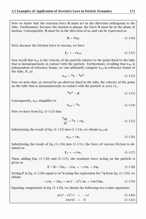
3.5 Examples of Application of Newton’s Laws in Particle Dynamics 171
Now we know that the reaction force N must act in the direction orthogonal to thetube. Furthermore, because the motion is planar, the force N must lie in the plane ofmotion. Consequently, N must lie in the direction of eθ and can be expressed as
N = Neθ (3–130)
Next, because the friction force is viscous, we have
Ff = −cvrel (3–131)
Now recall that vrel is the velocity of the particle relative to the point fixed to the tubethat is instantaneously in contact with the particle. Furthermore, recalling that vrel isindependent of reference frame, we can arbitrarily compute vrel in reference frame ofthe tube, R, as
vrel = Rv−RvR (3–132)
Now we note that, as viewed by an observer fixed to the tube, the velocity of the pointon the tube that is instantaneously in contact with the particle is zero, i.e.,
RvR = 0 (3–133)
Consequently, vrel simplifies to
vrel = Rv (3–134)
Now we have from Eq. (3–123) that
Rdrdt
= Rv = rer (3–135)
Substituting the result of Eq. (3–135) into (3–134), we obtain vrel as
vrel = rer (3–136)
Substituting the result of Eq. (3–136) into (3–131), the force of viscous friction is ob-tained as
Ff = −crer (3–137)
Then, adding Eqs. (3–130) and (3–137), the resultant force acting on the particle isgiven as
F = N = Neθ − crer = −crer +Neθ (3–138)
Setting F in Eq. (3–138) equal to mFa using the expression for Fa from Eq. (3–129), weobtain
−crer +Neθ =m(r −Ω2r)er + 2mrΩeθ (3–139)
Equating components in Eq. (3–139), we obtain the following two scalar equations:
m(r −Ω2r) = −cr (3–140)
2mrΩ = N (3–141)
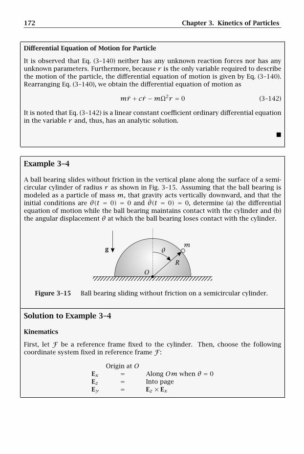
172 Chapter 3. Kinetics of Particles
Differential Equation of Motion for Particle
It is observed that Eq. (3–140) neither has any unknown reaction forces nor has anyunknown parameters. Furthermore, because r is the only variable required to describethe motion of the particle, the differential equation of motion is given by Eq. (3–140).Rearranging Eq. (3–140), we obtain the differential equation of motion as
mr + cr −mΩ2r = 0 (3–142)
It is noted that Eq. (3–142) is a linear constant coefficient ordinary differential equationin the variable r and, thus, has an analytic solution.
Example 3–4
A ball bearing slides without friction in the vertical plane along the surface of a semi-circular cylinder of radius r as shown in Fig. 3–15. Assuming that the ball bearing ismodeled as a particle of mass m, that gravity acts vertically downward, and that theinitial conditions are θ(t = 0) = 0 and θ(t = 0) = 0, determine (a) the differentialequation of motion while the ball bearing maintains contact with the cylinder and (b)the angular displacement θ at which the ball bearing loses contact with the cylinder.
gm
OR
θ
Figure 3–15 Ball bearing sliding without friction on a semicircular cylinder.
Solution to Example 3–4
Kinematics
First, let F be a reference frame fixed to the cylinder. Then, choose the followingcoordinate system fixed in reference frame F :
Origin at OEx = Along Om when θ = 0Ez = Into pageEy = Ez × Ex
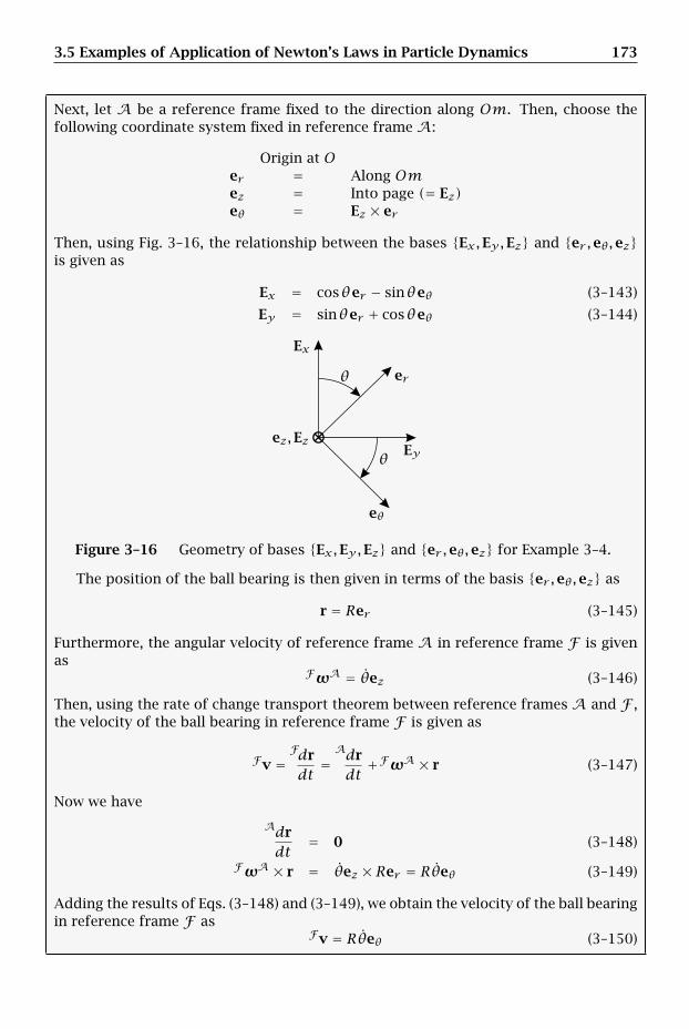
3.5 Examples of Application of Newton’s Laws in Particle Dynamics 173
Next, let A be a reference frame fixed to the direction along Om. Then, choose thefollowing coordinate system fixed in reference frame A:
Origin at Oer = Along Omez = Into page (= Ez)eθ = Ez × er
Then, using Fig. 3–16, the relationship between the bases Ex,Ey,Ez and er ,eθ,ezis given as
Ex = cosθer − sinθeθ (3–143)
Ey = sinθer + cosθeθ (3–144)
⊗
er
eθ
Ex
Eyez,Ez
θ
θ
Figure 3–16 Geometry of bases Ex,Ey,Ez and er ,eθ,ez for Example 3–4.
The position of the ball bearing is then given in terms of the basis er ,eθ,ez as
r = Rer (3–145)
Furthermore, the angular velocity of reference frame A in reference frame F is givenas
FωA = θez (3–146)
Then, using the rate of change transport theorem between reference frames A and F ,the velocity of the ball bearing in reference frame F is given as
Fv =Fdrdt
=Adrdt+FωA × r (3–147)
Now we have
Adrdt
= 0 (3–148)
FωA × r = θez × Rer = Rθeθ (3–149)
Adding the results of Eqs. (3–148) and (3–149), we obtain the velocity of the ball bearingin reference frame F as
Fv = Rθeθ (3–150)
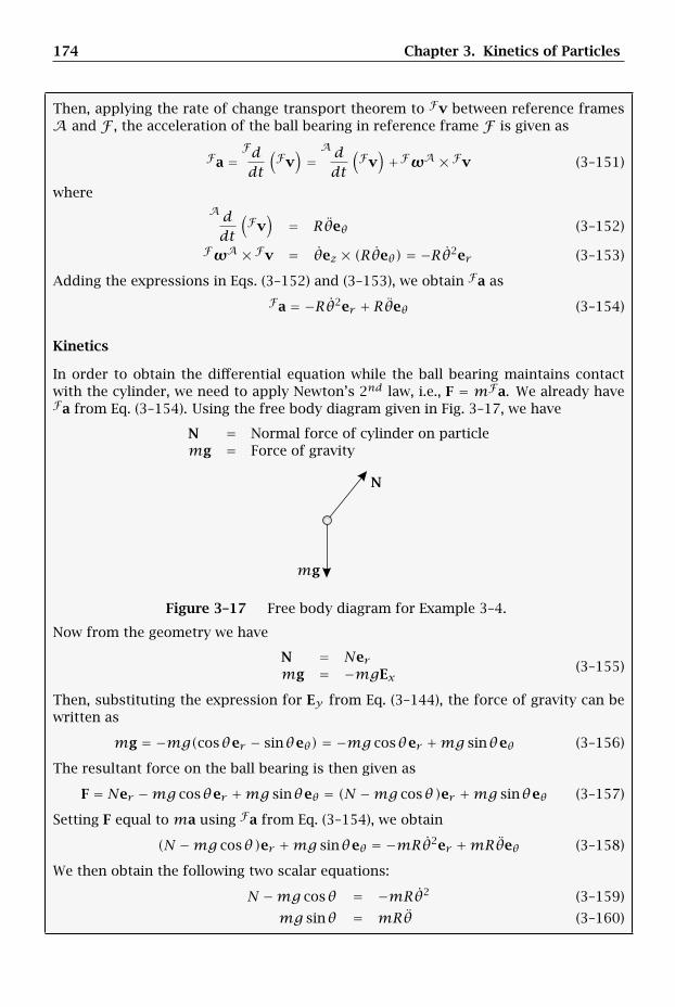
174 Chapter 3. Kinetics of Particles
Then, applying the rate of change transport theorem to Fv between reference framesA and F , the acceleration of the ball bearing in reference frame F is given as
Fa =Fddt
(Fv)=A ddt
(Fv)+FωA × Fv (3–151)
whereA ddt
(Fv)
= Rθeθ (3–152)
FωA × Fv = θez × (Rθeθ) = −Rθ2er (3–153)
Adding the expressions in Eqs. (3–152) and (3–153), we obtain Fa asFa = −Rθ2er + Rθeθ (3–154)
Kinetics
In order to obtain the differential equation while the ball bearing maintains contactwith the cylinder, we need to apply Newton’s 2nd law, i.e., F = mFa. We already haveFa from Eq. (3–154). Using the free body diagram given in Fig. 3–17, we have
N = Normal force of cylinder on particlemg = Force of gravity
N
mg
Figure 3–17 Free body diagram for Example 3–4.
Now from the geometry we have
N = Nermg = −mgEx
(3–155)
Then, substituting the expression for Ey from Eq. (3–144), the force of gravity can bewritten as
mg = −mg(cosθer − sinθeθ) = −mg cosθer +mg sinθeθ (3–156)
The resultant force on the ball bearing is then given as
F = Ner −mg cosθer +mg sinθeθ = (N −mg cosθ)er +mg sinθeθ (3–157)
Setting F equal to ma using Fa from Eq. (3–154), we obtain
(N −mg cosθ)er +mg sinθeθ = −mRθ2er +mRθeθ (3–158)
We then obtain the following two scalar equations:
N −mg cosθ = −mRθ2 (3–159)
mg sinθ = mRθ (3–160)
3.5 Examples of Application of Newton’s Laws in Particle Dynamics 175
(a) Differential Equation While Ball Bearing Maintains Contact with Cylinder
Noticing that Eq. (3–160) has no reaction forces, we obtain the differential equation ofmotion for the ball bearing while it maintains contact with the cylinder as
mRθ =mg sinθ (3–161)
Simplifying Eq. (3–161), we obtain
θ = gR
sinθ (3–162)
(b) Angular Displacement at Which Ball Bearing Loses Contact with Cylinder
We note that the ball bearing will lose contact with the cylinder when the reaction forceis zero, i.e., when N = 0. Setting N equal to zero in Eq. (3–159), we obtain
−mg cosθ = −mRθ2 (3–163)
which implies that
θ2 = gR
cosθ (3–164)
Now it is observed that Eq. (3–164) is not an algebraic equation in θ because it containsa term of θ2. Therefore, we need to find an expression for θ2 in terms of θ. Such anexpression is obtained by solving the differential equation of Eq. (3–162). First, we notethat
θ = dθdt
= dθdθdθdt
= θ dθdθ
(3–165)
Substituting θ into Eq. (3–162), we obtain
θdθdθ
= gR
sinθ (3–166)
Separating variables in Eq. (3–166), we obtain
θdθ = gR
sinθdθ (3–167)
Integrating both sides of Eq. (3–167) gives
∫ θθ0
ηdη =∫ θθ0
gR
sinνdν (3–168)
where η and ν are dummy variables of integration. Using the initial conditions θ(t =0) = 0 and θ(t = 0) = 0, Eq. (3–168) simplifies to
θ2
2= gR(1− cosθ) (3–169)
from which we obtain
θ2 = 2gR(1− cosθ) (3–170)
176 Chapter 3. Kinetics of Particles
Substituting θ2 from Eq. (3–170) into (3–164), we obtain
2gR(1− cosθ) = g
Rcosθ (3–171)
Dropping the common factor of g/R and rearranging Eq. (3–171) to solve for cosθ , weobtain
cosθ = 2/3 (3–172)
Consequently, the angular displacement at which the ball bearing loses contact withthe cylinder is
θ = cos−1 (2/3) ≈ 48.1897 deg (3–173)
3.6 Linear Momentum and Linear Impulse for a Particle
3.6.1 Linear Momentum of a Particle
Let P be a particle of mass m moving in an inertial reference frame N . Furthermore,let r be the position of P and let Nv be the velocity of the particle in N . Then thelinear momentum of the particle in reference frame N , denoted NG, is defined as
NG ≡ G =mNv (3–174)
Computing the rate of change of NG in reference frame N , we have
Nddt
(NG
)=Nddt
(mNv
)=m
Nddt
(Nv
)=mNa (3–175)
Then, applying Newton’s 2nd law of Eq. (3–41), we have
F =Nddt
(NG
)(3–176)
Equation (3–176) states that the resultant force acting on a particle of massm is equalto the rate of change of linear momentum in an inertial reference frame N . We notethat Eq. (3–176) is an alternate form of Newton’s 2nd law.
3.6.2 Principle of Linear Impulse and Momentum for a Particle
Let P be a particle of mass m moving in an inertial reference frame N . Furthermore,let F be a force acting on P . Suppose now that we consider the effect of the force ona given time interval t ∈ [t1, t2]. Then the integral of the force from t1 to t2 > t1,denoted F, is given as
F =∫ t2t1
Fdt (3–177)
3.6 Linear Momentum and Linear Impulse for a Particle 177
The quantity F is called the linear impulse of the force F on the time interval t ∈ [t1, t2].Then, integrating both sides of Eq. (3–176) from t1 to t2, we have
∫ t2t1
Fdt =∫ t2t1
Nddt
(NG
)dt = NG(t2)−NG(t1) (3–178)
Furthermore, applying the definition of linear impulse using Eq. (3–177), Eq. (3–178)can be written as
F = NG(t2)−NG(t1) (3–179)
Equation (3–179) is called the principle of linear impulse and linear momentum andstates that the change in linear momentum of a particle over a specified time intervalis equal to the total linear impulse of the external forces acting on the particle duringthe same time interval. In terms of the velocity of the particle in the inertial referenceframe N , Eq. (3–179) can be written as
F =mNv(t2)−mNv(t1) (3–180)
3.6.3 Conservation of Linear Momentum
Let NG be the linear momentum of a particle in an inertial reference frame N and letu be a unit vector in R3. Then NG is said to be conserved in the direction of u if
NG · u = constant (3–181)
Observing that NG · u is a scalar function, we can differentiate Eq. (3–181) to obtain
ddt
(NG · u
)= 0 (3–182)
Again, because NG·u is a scalar function, we can compute its rate of change arbitrarilyin reference frame N using the product rule for differentiation to obtain
ddt
(NG · u
)=Nddt
(NG
)· u+NG ·
Ndudt
= 0 (3–183)
Substituting the result of Eq. (3–176) into (3–183), the linear momentum of a particlewill be conserved in the direction of u if and only if
F · u+NG ·Ndudt
= 0 (3–184)
Finally, we say that the linear momentum of a particle NG is conserved in all directionsor, more simply, the linear momentum NG is conserved, if
NG = constant (3–185)
where in this case the constant is a vector. Differentiating Eq. (3–185) in the inertialreference frame N , we obtain
Nddt
(NG
)= 0 (3–186)
178 Chapter 3. Kinetics of Particles
It is seen that if Eq. (3–186) is satisfied, then from Eq. (3–176) we have that linearmomentum is conserved if
F = 0 (3–187)
In other words, the linear momentum of a particle will be conserved (in all directions)if the resultant force acting on the particle is zero. It is important to keep in mindthat for most problems there may only exist certain directions along which the linearmomentum is conserved. In such cases these directions must be determined by apply-ing Eq. (3–184). However, for some problems linear momentum may be conserved inall directions. Determining if linear momentum is conserved in all directions is mostconveniently determined by applying Eq. (3–187).
Suppose now that we consider the case where u is a direction that is fixed in theinertial reference frame N , i.e.,
Ndudt
= 0 (3–188)
Applying Eq. (3–188), Eq. (3–184) reduces to
F · u = 0 (3–189)
Equation (3–189) states that the linear momentum of a particle in an inertial referenceframe N will be conserved in the inertially fixed direction u if the component of forceacting on the particle in the direction of u is zero.
3.7 Moment of a Force and Moment Transport Theorem for a Particle
Let F be a force acting on a particle P of mass m. Furthermore, let r be the position ofthe particle and let Q be an arbitrary point. Then the moment of the force F relative topoint Q, denoted MQ, is defined as
MQ = (r− rQ)× F (3–190)
Suppose now that we consider another arbitrary point Q′. Then, from Eq. (3–190), themoment applied by the force F relative to Q′ is
MQ′ = (r− rQ′)× F (3–191)
Then, subtracting Eq. (3–191) from (3–190), we have
MQ −MQ′ = (r− rQ)× F− (r− rQ′)× F (3–192)
Equation (3–192) simplifies to
MQ −MQ′ = (rQ′ − rQ)× F (3–193)
Rearranging Eq. (3–193), we obtain
MQ = MQ′ + (rQ′ − rQ)× F (3–194)
Equation (3–194) is called the moment transport theorem for a particle and relates themoment due to a force F relative to an arbitrary point Q to the moment of that sameforce relative to any other point Q′.
3.8 Angular Momentum and Angular Impulse for a Particle 179
3.8 Angular Momentum and Angular Impulse for a Particle
3.8.1 Angular Momentum and Its Rate of Change of a Particle
Let P be a particle of mass m moving in an inertial reference frame N . Furthermore,let r be the position of the particle, let Nv be the velocity of the particle in N , andlet Q be an arbitrary point. Then the angular momentum of the particle in an inertialreference frame N relative to point Q is defined as7
NHQ = (r− rQ)×m(Nv−NvQ) (3–195)
Computing the rate of change of NHQ in the inertial reference frame N , we have
Nddt
(NHQ
)=Nddt
[(r− rQ)×m(Nv−NvQ)
](3–196)
Expanding Eq. (3–196), we obtain
Nddt
(NHQ
)=Nddt(r− rQ)×m(Nv−NvQ)
+ (r− rQ)×mNddt
(Nv−NvQ
) (3–197)
Now we note thatNddt(r− rQ) = Nv−NvQ
Nddt
(Nv−NvQ
)= Na−NaQ
(3–198)
Furthermore,(Nv−NvQ)×m(Nv−NvQ) = 0 (3–199)
Equation (3–197) then simplifies to
Nddt
(NHQ
)= (r− rQ)×m
(Na−NaQ
)(3–200)
Then, applying Newton’s 2nd law of Eq. (3–41), Eq. (3–200) can be rewritten as
Nddt
(NHQ
)= (r− rQ)× F− (r− rQ)×mNaQ (3–201)
Using the definition of the moment of a force from Eq. (3–190), we see that
(r− rQ)× F = MQ (3–202)
7There are two conventions for the definition of angular momentum. The first convention, shown inEq. (3–195), uses the relative velocity Nv − NvQ between the particle and the reference point while thesecond convention uses the (absolute) velocity of the particle Nv. Either of the aforementioned conven-tions is perfectly valid, but the convention using relative velocity is adopted here because the author feelsthat the results obtained using relative velocity are more intuitive than the results obtained using absolutevelocity. Examples of previous works that define angular momentum using the relative velocity conven-tion include Greenwood (1977; 1988) while examples of works that define angular momentum using theabsolute velocity convention include Synge and Griffith (1959), O’Reilly (2001), and Thornton and Marion(2004).

180 Chapter 3. Kinetics of Particles
where MQ is the moment of the resultant force F acting on the particle relative to pointQ. Consequently, Eq. (3–201) can be written as
Nddt
(NHQ
)= MQ − (r− rQ)×mNaQ (3–203)
The quantity−(r− rQ)×mNaQ (3–204)
in Eq. (3–203) is called the inertial moment of point Q relative to point P .Now suppose that we choose a reference pointO that is fixed in an inertial reference
frame N . Then the acceleration of point O in N is zero, i.e., NaO = 0, which impliesthat the inertial moment, −(r − rO) ×mNaO , is zero. Consequently, for a referencepoint O fixed in an inertial reference frame N , Eq. (3–203) reduces to
Nddt
(NHO
)= MO (3–205)
Equation (3–205) states that the rate of change of angular momentum of a particlerelative to a reference point O that is fixed in an inertial reference frame is equal tothe moment due to all external forces relative to point O.
3.8.2 Principle of Angular Impulse and Angular Momentum of a Particle
Now consider an interval of time t ∈ [t1, t2]. Then the integral of the moment MQ fromt1 to t2, denoted MQ, is given as
MQ =∫ t2t1
MQdt (3–206)
The quantity MQ is called the angular impulse of the moment MQ on the time intervalt ∈ [t1, t2]. Integrating both sides of Eq. (3–203) from t1 to t2, we obtain
∫ t2t1
[MQ − (r− rQ)×mNaQ
]dt =
∫ t2t1
[Nddt
(NHQ
)]dt (3–207)
Equation (3–207) can be rewritten as
∫ t2t1
MQdt −∫ t2t1(r− rQ)×mNaQdt =
∫ t2t1
[Nddt
(NHQ
)]dt (3–208)
Then, using Eqs. (3–206) and (3–207) and observing that
∫ t2t1
Nddt
(NHQ
)dt = NHQ(t2)−NHQ(t1) (3–209)
Eq. (3–207) simplifies to
MQ −∫ t2t1
[(r− rQ)×mNaQ
]dt = NHQ(t2)−NHQ(t1) (3–210)
3.8 Angular Momentum and Angular Impulse for a Particle 181
Equation (3–210) is called the principle of angular impulse and angular momentumrelative to an arbitrary reference point Q and states that the change in angular mo-mentum of a particle relative to an arbitrary reference point Q over a time intervalt ∈ [t1, t2] is equal to the sum of the angular impulse due to all external forces appliedto the particle relative to point Q and the angular impulse due to the inertial momentof point Q relative to point P on the time interval t ∈ [t1, t2].
Suppose now that we choose a reference pointO that is fixed in an inertial referenceframe. Then the acceleration of point O is zero, i.e., NaO = 0. Moreover, the secondterm in Eq. (3–210) is zero and Eq. (3–210) reduces to
MO = NHO(t2)−NHO(t1) (3–211)
Equation (3–211) is called the principle of angular impulse and angular momentumrelative to a point O fixed in an inertial reference frame and states that the changein angular momentum of a particle relative to a point O fixed in an inertial referenceframe is equal to the angular impulse due to all external forces applied to the particlerelative to point O.
3.8.3 Conservation of Angular Momentum
Let NHQ be the angular momentum of a particle P in an inertial reference frame Nrelative to an arbitrary reference pointQ. Furthermore, let u be an arbitrary unit vectorin R3. Then the angular momentum NHQ is said to be conserved in the direction of uif
NHQ · u = constant (3–212)
Observing that NHQ · u is a scalar function, we can differentiate Eq. (3–212) to obtain
ddt
(NHQ · u
)= 0 (3–213)
Again, because NHQ · u is a scalar function, its rate of change is independent of ref-erence frame. Consequently, NHQ · u can be differentiated arbitrarily in the inertialreference frame N to give
Nddt
(NHQ · u
)=Nddt
(NHQ
)· u+NHQ ·
Ndudt
(3–214)
Then, using the result of Eq. (3–203), Eq. (3–214) can be written as
(MQ − (r− rQ)×mNaQ
)· u+NHQ ·
Ndudt
= 0 (3–215)
Consequently, the angular momentum NHQ in an inertial reference frame N will beconserved in the direction of u if and only if Eq. (3–215) is satisfied. Finally, we say thatthe angular momentum of a particle relative to an arbitrary pointQ, NHQ, is conservedin all directions or, more simply, is conserved, if
NHQ = constant (3–216)
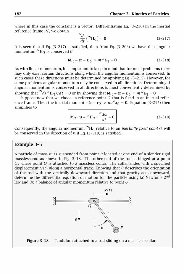
182 Chapter 3. Kinetics of Particles
where in this case the constant is a vector. Differentiating Eq. (3–216) in the inertialreference frame N , we obtain
Nddt
(NHQ
)= 0 (3–217)
It is seen that if Eq. (3–217) is satisfied, then from Eq. (3–203) we have that angularmomentum NHQ is conserved if
MQ − (r− rQ)×mNaQ = 0 (3–218)
As with linear momentum, it is important to keep in mind that for most problems theremay only exist certain directions along which the angular momentum is conserved. Insuch cases these directions must be determined by applying Eq. (3–215). However, forsome problems angular momentum may be conserved in all directions. Determining ifangular momentum is conserved in all directions is most conveniently determined by
showing thatNd(NHQ)/dt = 0 or by showing that MQ − (r− rQ)×mNaQ = 0
Suppose now that we choose a reference point O that is fixed in an inertial refer-ence frame. Then the inertial moment −(r − rO) ×mNaO = 0. Equation (3–215) thensimplifies to
MO · u+NHO ·Ndudt
= 0 (3–219)
Consequently, the angular momentum NHO relative to an inertially fixed point O willbe conserved in the direction of u if Eq. (3–219) is satisfied.
Example 3–5
A particle of mass m is suspended from point P located at one end of a slender rigidmassless rod as shown in Fig. 3–18. The other end of the rod is hinged at a pointQ, where point Q is attached to a massless collar. The collar slides with a specifieddisplacement x(t) along a horizontal track. Knowing that θ describes the orientationof the rod with the vertically downward direction and that gravity acts downward,determine the differential equation of motion for the particle using (a) Newton’s 2nd
law and (b) a balance of angular momentum relative to point Q.
x(t)
gl
m P
Q
θ
Figure 3–18 Pendulum attached to a rod sliding on a massless collar.
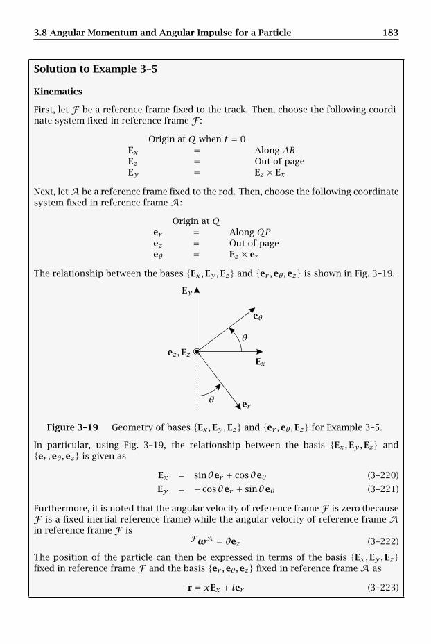
3.8 Angular Momentum and Angular Impulse for a Particle 183
Solution to Example 3–5
Kinematics
First, let F be a reference frame fixed to the track. Then, choose the following coordi-nate system fixed in reference frame F :
Origin at Q when t = 0Ex = Along ABEz = Out of pageEy = Ez × Ex
Next, letA be a reference frame fixed to the rod. Then, choose the following coordinatesystem fixed in reference frame A:
Origin at Qer = Along QPez = Out of pageeθ = Ez × er
The relationship between the bases Ex,Ey,Ez and er ,eθ,ez is shown in Fig. 3–19.
er
eθ
Ex
Ey
ez,Ez
θ
θ
Figure 3–19 Geometry of bases Ex,Ey,Ez and er ,eθ,Ez for Example 3–5.
In particular, using Fig. 3–19, the relationship between the basis Ex,Ey,Ez ander ,eθ,ez is given as
Ex = sinθer + cosθeθ (3–220)
Ey = − cosθer + sinθeθ (3–221)
Furthermore, it is noted that the angular velocity of reference frame F is zero (becauseF is a fixed inertial reference frame) while the angular velocity of reference frame Ain reference frame F is
FωA = θez (3–222)
The position of the particle can then be expressed in terms of the basis Ex,Ey,Ezfixed in reference frame F and the basis er ,eθ,ez fixed in reference frame A as
r = xEx + ler (3–223)
184 Chapter 3. Kinetics of Particles
Now letrQ = xExrP/Q = ler
(3–224)
Then the position of the particle can be written as
r = rQ + rP/Q (3–225)
Computing the rate of change of r in the inertial reference frame F , we have
Fv =Fdrdt
=Fddt
(rQ)+ Fd
dt(rP/Q
) = FvQ + FvP/Q (3–226)
Now, because F is fixed, we have
FvQ =Fddt
(rQ) = xEx (3–227)
Furthermore,
FvP/Q =Fddt
(rP/Q
) = A ddt
(rP/Q
)+FωA × rQ = θez × ler = lθeθ (3–228)
Adding the expressions in Eqs. (3–227) and (3–228), we obtain
Fv = xEx + lθeθ (3–229)
The acceleration of the particle in reference frame F is then obtained as
Fa = Fv =Fddt
(FvQ
)+Fddt
(FvP/Q
)= FaQ + FaP/Q (3–230)
First, using the result of Eq. (3–227), we have
FaQ =Fddt
(FvQ
)= xEx (3–231)
Next, applying the rate of change transport theorem of Eq. (2–128) on page 47 betweenreference frames A and F to FvP/Q using the result of Eq. (3–228), we obtain
FaP/Q =Fddt
(FvP/Q
)=A ddt
(FvP/Q
)+FωA × FvP/Q
= lθeθ + θez × lθeθ = −lθ2er + lθeθ
(3–232)
Adding the results of Eqs. (3–231) and (3–232), we obtain the acceleration of the parti-cle in reference frame F as
Fa = xEx − lθ2er + lθeθ (3–233)
Finally, substituting the expression for Ex in terms of er and eθ from Eq. (3–220), weobtain Fa in terms of the basis er ,eθ,ez as
Fa = x(sinθer + cosθeθ)− lθ2er + lθeθ (3–234)
Simplifying Eq. (3–234) gives
Fa = (x sinθ − lθ2)er + (x cosθ + lθ)eθ (3–235)
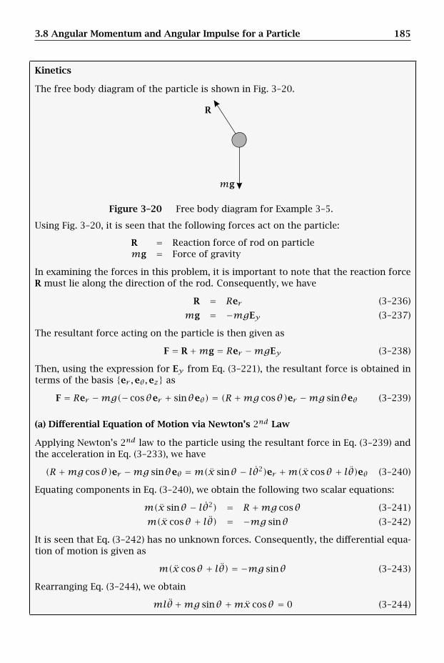
3.8 Angular Momentum and Angular Impulse for a Particle 185
Kinetics
The free body diagram of the particle is shown in Fig. 3–20.
R
mg
Figure 3–20 Free body diagram for Example 3–5.
Using Fig. 3–20, it is seen that the following forces act on the particle:
R = Reaction force of rod on particlemg = Force of gravity
In examining the forces in this problem, it is important to note that the reaction forceR must lie along the direction of the rod. Consequently, we have
R = Rer (3–236)
mg = −mgEy (3–237)
The resultant force acting on the particle is then given as
F = R+mg = Rer −mgEy (3–238)
Then, using the expression for Ey from Eq. (3–221), the resultant force is obtained interms of the basis er ,eθ,ez as
F = Rer −mg(− cosθer + sinθeθ) = (R +mg cosθ)er −mg sinθeθ (3–239)
(a) Differential Equation of Motion via Newton’s 2nd Law
Applying Newton’s 2nd law to the particle using the resultant force in Eq. (3–239) andthe acceleration in Eq. (3–233), we have
(R +mg cosθ)er −mg sinθeθ =m(x sinθ − lθ2)er +m(x cosθ + lθ)eθ (3–240)
Equating components in Eq. (3–240), we obtain the following two scalar equations:
m(x sinθ − lθ2) = R +mg cosθ (3–241)
m(x cosθ + lθ) = −mg sinθ (3–242)
It is seen that Eq. (3–242) has no unknown forces. Consequently, the differential equa-tion of motion is given as
m(x cosθ + lθ) = −mg sinθ (3–243)
Rearranging Eq. (3–244), we obtain
mlθ +mg sinθ +mx cosθ = 0 (3–244)
186 Chapter 3. Kinetics of Particles
(b) Differential Equation via Balance of Angular Momentum Relative to Point Q
We note that point Q is not inertially fixed and, thus, is an arbitrary point. Therefore,it is necessary to apply the moment balance for an arbitrary reference point as givenin Eq. (3–203), i.e., we need to apply
Fddt
(FHQ
)= MQ − (r− rQ)×mFaQ (3–245)
Now, because R passes through point Q, the moment relative to point Q is due purelyto gravity and is given as
MQ = (rg − rQ)×mg (3–246)
Furthermore, because the force of gravity acts at the location of the particle, we havethat
rg = r = xEx + ler (3–247)
Now, because rQ = xEx , we have
rg − rQ = ler (3–248)
The moment relative to point Q is then given as
MQ = ler × (−mgEy) = −mgler × Ey (3–249)
Then, using Eq. (3–221), we have er × Ey as
er × Ey = er × (− cosθer + sinθeθ) = sinθez (3–250)
Using Eq. (3–250), the moment relative to point Q simplifies to
MQ = −mgl sinθez (3–251)
Next, using rQ from Eq. (3–224), we have
r− rQ = rP/Q = ler (3–252)
Then, since FaQ = rQ = xEx , the inertial moment is given as
−(r− rQ)×mFaQ = −ler ×mxEx = −mlxer × Ex (3–253)
Using Eq. (3–220), we obtain er × Ex as
er × Ex = er × (sinθer + cosθeθ) = cosθez (3–254)
The inertial moment relative to point Q then simplifies to
−(r− rQ)×mFaQ = −mlx cosθez (3–255)
Finally, the rate of change of angular momentum relative to point Q is given as
Fddt
(FHQ
)= (r− rQ)×m(a− aQ) (3–256)
3.9 Instantaneous Linear and Angular Impulse 187
Noting thatFa− FaQ = −lθ2er + lθeθ (3–257)
and using the expression for r − rQ from Eq. (3–252), we obtain the rate of change ofangular momentum relative to point Q as
Fddt
(FHQ
)= ler ×m(−lθ2er + lθeθ) =ml2θez (3–258)
Then, substituting the results of Eqs. (3–251), (3–255), and (3–258) into (3–245), weobtain
ml2θez = −mgl sinθez −mlx cosθez (3–259)
Rearranging and simplifying Eq. (3–259), we obtain the differential equation as
mlθ +mg sinθ +mx cosθ = 0 (3–260)
It is noted that the result of Eq. (3–260) obtained using a balance of angular momentumrelative to point Q is identical to that of Eq. (3–244) obtained using Newton’s 2nd law.
3.9 Instantaneous Linear and Angular Impulse
In many applications in dynamics, impulses are assumed to occur without the passageof time. In order for an impulse to have a nonzero value over a zero time interval,it is necessary that the force be infinite. While strictly speaking it is not possible toapply an infinite force, such an assumption is often a good approximation to reality.Modeling an infinite force over a zero time interval is accomplished by introducinga special function called the Dirac delta function. The Dirac delta function, denotedδ(t − s), is defined as follows:
δ(t − s) =
0 , t ≠ s∞ , t = s (3–261)
Furthermore, δ(t − s) has the following property:∫∞−∞f(t)δ(t − s)dt = f(s) (3–262)
From Eq. (3–262) it is seen that if f(t) = 1, then∫∞−∞δ(t − s)dt = 1 (3–263)
where f(t) is an arbitrary function of t. Suppose now that we have an infinite force Fmodeled as follows:
F(t) = Fδ(t − τ) (3–264)
where F is finite. Suppose now that we consider the instant of time t = τ . ApplyingEq. (3–177), the linear impulse of the force F is given as
F =∫ t=τ+t=τ−
F(t)dt =∫∞−∞
F(t)dt (3–265)
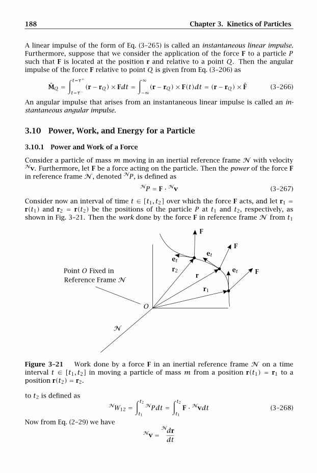
188 Chapter 3. Kinetics of Particles
A linear impulse of the form of Eq. (3–265) is called an instantaneous linear impulse.Furthermore, suppose that we consider the application of the force F to a particle Psuch that F is located at the position r and relative to a point Q. Then the angularimpulse of the force F relative to point Q is given from Eq. (3–206) as
MQ =∫ t=τ+t=τ−
(r− rQ)× Fdt =∫∞−∞(r− rQ)× F(t)dt = (r− rQ)× F (3–266)
An angular impulse that arises from an instantaneous linear impulse is called an in-stantaneous angular impulse.
3.10 Power, Work, and Energy for a Particle
3.10.1 Power and Work of a Force
Consider a particle of mass m moving in an inertial reference frame N with velocityNv. Furthermore, let F be a force acting on the particle. Then the power of the force Fin reference frame N , denoted NP , is defined as
NP = F · Nv (3–267)
Consider now an interval of time t ∈ [t1, t2] over which the force F acts, and let r1 =r(t1) and r2 = r(t2) be the positions of the particle P at t1 and t2, respectively, asshown in Fig. 3–21. Then the work done by the force F in reference frame N from t1
Point O Fixed in
N
Reference Frame N
etet
et F
F
F
r
r1
r2
O
Figure 3–21 Work done by a force F in an inertial reference frame N on a timeinterval t ∈ [t1, t2] in moving a particle of mass m from a position r(t1) = r1 to aposition r(t2) = r2.
to t2 is defined asNW12 =
∫ t2t1
NPdt =∫ t2t1
F · Nvdt (3–268)
Now from Eq. (2–29) we have
Nv =Ndrdt
3.10 Power, Work, and Energy for a Particle 189
Consequently, the work NW12 can be written as
NW12 =∫ t2t1
F ·Ndrdtdt =
∫ r2
r1
F · Ndr (3–269)
where Ndr is a differential change in the position of the particle in reference frameN .Now recall from Section 2.11.4 that the velocity of a particle can be written in terms ofthe tangent vector et as
Nv = Nvet
where Nv is the speed of the particle in reference frame N . The work in referenceframe N can then be written as
NW12 =∫ t2t1
F · Nvetdt (3–270)
It can be seen from Eq. (3–270) that only the component of the force F that lies in thedirection of Nv does any work; any component of F orthogonal to Nv does not con-tribute to the work. Furthermore, it is seen from Eq. (3–268) that, due to its dependenceon Nv, the work of a force F depends on the choice of the reference frame.
3.10.2 Kinetic Energy and Work-Energy Theorem for a Particle
The kinetic energy of a particle of mass m in an inertial reference frame N , denotedNT , is defined as
NT = 12m
Nv · Nv (3–271)
where Nv is the velocity of the particle in reference frame N . Noting that NT is ascalar function and, hence, is independent of reference frame, its rate of change isgiven as
ddt
(NT
)= 1
2mddt
[Nv · Nv
](3–272)
Differentiating the vectors on the right-hand side of Eq. (3–272) in reference frame N ,we obtain
ddt
(NT
)= 1
2m[Nddt
(Nv
)· Nv+Nv ·
Nddt
(Nv
)](3–273)
Furthermore, noting thatNd(Nv)/dt = Na and using the fact that the scalar product
is commutative, we obtainddt
(NT
)=mNa · Nv (3–274)
Then, applying Newton’s 2nd law of Eq. (3–41), Eq. (3–274) becomes
ddt
(NT
)= F · Nv = NP (3–275)
where NP is the power of the force F in an inertial reference frame N as defined inEq. (3–267). Equation (3–275) is called the work-energy theorem for a particle and re-lates the rate of change of kinetic energy of a particle in an inertial reference frame Nto the power of the resultant force acting on the particle. It is important to understandthat Eq. (3–275) is valid only in an inertial reference frame.
190 Chapter 3. Kinetics of Particles
3.10.3 Principle of Work and Energy for a Particle
Now suppose that we consider motion over a time interval t ∈ [t1, t2]. IntegratingEq. (3–275) from t1 to t2, we have
∫ t2t1
ddt
(NT
)dt =
∫ t2t1
F · Nvdt (3–276)
Now we know from Eq. (3–268) that the work done by all forces acting on the particleon the interval t ∈ [t1, t2] is given as
NW12 =∫ t2t1
F · Nvdt (3–277)
Furthermore, we have
∫ t2t1
ddt
(NT
)dt = NT(t2)−NT(t1) = NT2 −NT1 (3–278)
Using Eq. (3–277) together with Eq. (3–278), we obtain
NT2 −NT1 = NW12 (3–279)
Equation (3–279) is called the principle of work and energy for a particle and states thatthe change in kinetic energy between any two points along the trajectory of a particlein an inertial reference frame is equal to the work done by all forces acting on theparticle between those same two points.
3.10.4 Conservative Forces and Potential Energy
It is seen from Eq. (3–268) that, in general, the work done by a force F over a timeinterval t ∈ [t1, t2] depends on both the trajectory taken by the particle on [t1, t2] andthe position of the particle at the endpoints t1 and t2. Consider now a force Fc whosework in moving a particle from an initial position r(t1) = r1 to a final position r2(t2) =r2 does not depend on the trajectory taken by the particle but, instead, depends ononly the endpoints r1 and r2. Then the force Fc is said to be a conservative force. Aschematic of a conservative force Fc is shown in Fig. 3–22.Suppose now that Nv(1), . . . ,Nv(n) are the velocities in an inertial reference frame Nthat correspond to an arbitrary set of trajectories that start at r1 and end at r2. Thenthe force Fc is conservative if the work done from r1 to r2 is the same for all trajectoriesNv(i) i = 1,2, . . . , n, i.e.,
NWc12 =
∫ t2t1
Fc · Nv(1) = · · · =∫ t2t1
Fc · Nv(n) (3–280)
A consequence of the fact that a conservative force is independent of the trajectory isthat there exists a scalar function NU = NU(r) such that
Fc = −∇rNU = − ∂
∂r
(NU
)(3–281)

3.10 Power, Work, and Energy for a Particle 191
Fc
Fc
Fc
Trajectories That PassThrough r1 and r2
Point O Fixed in
N
Reference Frame N
r1
r2
O
Figure 3–22 Work done by a conservative force Fc in moving a particle from a po-sition r(t1) = r1 to a position r(t2) = r2. The work of the conservative force dependsonly on the endpoints r1 and r2 and does not depend on the trajectory subtended bythe particle in moving from r1 to r2.
where r is the vector that defines the location in R3 relative to a point O fixed inreference frame N at which the force Fc acts. The scalar function NU in Eq. (3–281)is called a potential energy of the force Fc in the inertial reference frame N and theoperator ∇r is the gradient with respect to r.8 Then, using the definition of power fromEq. (3–267), the power of the conservative force Fc in the inertial reference frame N ,denoted NPc , is given as
NPc = Fc · Nv = −∇rNU · Nv = − ∂
∂r
(NU
)· Nv (3–282)
Next, applying Eq. (2–22) to (3–282), we see that
∇rNU · Nv = d
dt
(NU
)(3–283)
Substituting the identity of Eq. (3–283) into (3–282), we obtain NPc as
NPc = − ddt
(NU
)(3–284)
Consequently, the power of a conservative force in an inertial reference frame N isthe negative of the rate of change of a potential energy of the conservative force wherepotential energy is computed in the inertial reference frame N .
Now consider a time interval t ∈ [t1, t2] over which the conservative force Fc acts.Using Eq. (3–282), the work done by the conservative force Fc in reference frame N
8We use the terminology “a potential energy” instead of “the potential energy” because all potentialenergies, up to an arbitrary function of time, have the same gradient with respect to position.
192 Chapter 3. Kinetics of Particles
from t1 to t2, denoted NWc12, is given as
NWc12 =
∫ t2t1− ddt
(NU
)dt = −
∫ NU2
NU1
dU (3–285)
Then, using the fact that r(t1) = r1 and r(t2) = r2, Eq. (3–285) can be rewritten as
NWc12 = NU(r(t1))−NU(r(t2)) = NU(r1)−NU(r2) (3–286)
It can be seen from Eq. (3–286) that, consistent with the property of Eq. (3–280), thework done by a conservative force Fc in reference frame N over a time interval t ∈[t1, t2] depends only upon the values of the position at the endpoints and, thus, isindependent of the trajectory taken by the particle.
Suppose now that several conservative forces Fc1, . . . ,Fcn act on a particle. Then eachforce has an associated potential energy NU1, . . . ,NUn, i.e.,
Fci = −∇rNUi (i = 1, . . . , n) (3–287)
Then the total potential energy of all conservative forces in the inertial reference frameN , denoted U , is defined as
NU =n∑i=1
NUi (3–288)
Correspondingly, the total conservative force acting on the particle is given as
Fc =n∑i=1
Fci = −n∑i=1
∇rNUi = −∇r
NU (3–289)
3.10.5 Examples of Conservative Forces
In this section we provide examples of several commonly encountered conservativeforces. These forces will be used extensively in the analysis of dynamics problems.
Constant Forces
Let c be a constant force. Then the potential energy of c in reference frameN , denotedNUc , is given as
NUc = −c · r (3–290)
To verify that NUc is in fact the potential energy of the constant force c, we can com-pute the rate of change of NUc as
ddt
(NUc
)= ∇r (−c · r) ·
Ndrdt
= −c · Nv (3–291)
where we note that, since c is constant, we have ∇ (c · r) ≡ c. Then, observing that−c · Nv is the negative of the power of the force c in the inertial reference frame N ,we obtain
NPc = c · Nv (3–292)
Therefore,NPc = − ddt
(NUc
)(3–293)
which implies that c is conservative.
3.10 Power, Work, and Energy for a Particle 193
Spring Forces
Recall from Eq. (3–19) that the force applied to a particle by a linear spring with springconstant K is given as
Fs = −K( − 0
)us (3–294)
where = ‖r− rQ‖ is the length of the spring, r is the position of the particle, and rQis the attachment point of the spring. Now let N be an inertial reference frame andassume that the attachment point is fixed in N , i.e., assume that
NvQ = 0
NaQ = 0(3–295)
Then the potential energy of a linear spring in reference frame N , denoted NUs , isgiven as
NUs = K2( − 0
)2 (3–296)
where = ‖r − rQ‖ and 0 are the stretched and unstretched length of the spring,respectively. To verify that NUs is the potential energy of Fs , we need to computed(NUs)/dt. Computing the rate of change of NUs , we have
ddt
(NUs
)= ddt
[K2
( − 0
)2]= K ( − 0
) ddt
( − 0
)(3–297)
Using the fact that = ‖r− rQ‖, we obtain
ddt
( − 0
) = ∇r−rQ
( − 0
) · Nddt
(r− rQ
)(3–298)
where the gradient is evaluated with respect to r− rQ. The gradient is given as
∇r−rQ
( − 0
) = ∇r−rQ‖r− rQ‖= N∇r−rQ
[(r− rQ
) · (r− rQ)]1/2
= r− rQ‖r− rQ‖
= r− rQ
(3–299)
Consequently,ddt
( − 0
) = r− rQ
·Nddt
(r− rQ
)(3–300)
The quantity d(NUs)/dt then becomes
ddt
(NUs
)= K ( − 0
) r− rQ
·Nddt
(r− rQ
)(3–301)
Now, because the attachment point is fixed in the inertial reference frame N , we have
Nddt
(r− rQ
) = Nv (3–302)
194 Chapter 3. Kinetics of Particles
Consequently,ddt
(NUs
)= K ( − 0
) r− rQ
· Nv (3–303)
Using the fact that (r− rQ)/ = us , Eq. (3–303) can be rewritten as
ddt
(NUs
)= −K ( − 0
)us · Nv (3–304)
Now we observe that Fs = −K( − 0
)us . Therefore, d(NUs)/dt simplifies to
ddt
(NUs
)= −Fs · Nv (3–305)
It is seen that the quantity Fs · Nv is the power of Fs in reference frame N , i.e.,
NPs = Fs · Nv (3–306)
Therefore,NPs = − ddt
(NUs
)(3–307)
which implies that Fs is conservative.
Gravitational Forces
Recall from Newton’s law of gravitation of Eq. (3–25) that the force of attraction of aparticle of mass M on a particle of mass m is given as
Fg = −GmMr 3r (3–308)
where r = r− rM is the position of m relative to M and r = ‖r‖. Furthermore, assumethat the position of M is inertially fixed, i.e., assume that
NvM = 0
NaM = 0(3–309)
Then the potential energy of a gravitational force, denoted Ug , is given as
NUg = −GmMr (3–310)
To verify that NUg is indeed the potential energy of a gravitational force, we computed(NUg)/dt as
ddt
(NUg
)= GmM
r 2
drdt
(3–311)
Now we note that, using the scalar product, an alternate expression for r is
r = √r · r = (r · r)1/2 (3–312)
Differentiating r in the inertial reference frame N using Eq. (3–312), we obtain
drdt
= r = 12(r · r)−1/2
[Ndrdt· r+ r ·
Ndrdt
](3–313)
3.10 Power, Work, and Energy for a Particle 195
Furthermore, because the mass M is inertially fixed, we have
N ddt
r = Nv−NvM = Nv (3–314)
Consequently, Eq. (3–313) simplifies to
r = 12(r · r)−1/2
[2Nv · r
]=
Nv · r√r · r
(3–315)
Furthermore, substituting Eq. (3–312) into (3–315), we obtain
r =Nv · rr
(3–316)
Then, substituting r from Eq. (3–316) into (3–311) gives
ddt
(NUg
)= GmM
r 2
Nv · rr
= GmMr 3
r · Nv (3–317)
Using the definition of the gravitational force from Eq. (3–308), Eq. (3–317) becomes
ddt
(NUg
)= −Fg · Nv (3–318)
Now we note that the power of a gravitational force in reference frame N , denoted Pg ,is given as Fg · Nv. Therefore,
NPg = − ddt(NUg
)(3–319)
which implies that Fg is conservative.
3.10.6 Alternate Form of Work-Energy Theorem for a Particle
Let r be the position of a particle and let Nv be the velocity of the particle in aninertial reference frame N . Consider now that the particle is being acted on by con-servative forces Fc1, . . . ,Fcn and a resultant nonconservative force Fnc . Furthermore, letNU1(r), . . . ,NUn(r) be the potential energies of Fc1, . . . ,Fcn, respectively, in the inertialreference frame N . Then
Fci = −∇rNUi (i = 1, . . . , n) (3–320)
The resultant conservative force acting on the particle, denoted Fc , is then given as
Fc =n∑i=1
Fci =n∑i=1
−∇rNUi (3–321)
The total potential energy in the inertial reference frame N is then obtained fromEq. (3–288) as
NU =n∑i=1
NUi (3–322)

196 Chapter 3. Kinetics of Particles
Consequently, the total conservative force acting on the particle is given as
Fc = −∇rNU (3–323)
Then the resultant force acting on the particle is given as
F = Fc + Fnc = −∇rNU + Fnc (3–324)
Now, from the work-energy theorem of Eq. (3–275), we have
ddt
(NT
)= F · Nv (3–325)
Substituting the expression from Eq. (3–324) into (3–325), we obtain
ddt
(NT
)=(∇r
NU + Fnc)· Nv (3–326)
Consequently,ddt
(NT
)= −∇r
(NU
)· Nv+ Fnc · Nv (3–327)
Now recall from Eq. (3–282) that
∇r
(NU
)· Nv = d
dt
(NU
)(3–328)
Equation (3–327) can then be written as
ddt
(NT
)= − d
dt
(NU
)+ Fnc · Nv (3–329)
Equation (3–329) can be rearranged to give
ddt
(NT +NU
)= Fnc · Nv (3–330)
The quantityNE = NT +NU (3–331)
is called the total energy in the inertial reference frameN . In terms of the total energy,we have
ddt
(NE
)= Fnc · Nv (3–332)
Equation (3–332) is an alternate form of the work-energy theorem and states that therate of change of the total energy for a particle in an inertial reference frame is equalto the power of the nonconservative forces in an inertial reference frame. Similar toprevious results involving the laws of kinetics, it is noted that Eq. (3–332) is valid onlyin an inertial reference frame.
3.10 Power, Work, and Energy for a Particle 197
3.10.7 Conservation of Energy for a Particle
Now suppose that the resultant nonconservative force Fnc does no work, i.e.,
Fnc · Nv = 0 (3–333)
Thenddt
(NE
)= 0 (3–334)
which implies thatNE = constant (3–335)
When the total energy of a particle is a constant in an inertial reference frame N , thetotal energy of the particle in N is said to be conserved. It is seen from Eqs. (3–333)and (3–334) that the total energy of a particle in an inertial reference frame N will beconserved only if the power produced by all nonconservative forces in N is zero.
3.10.8 Alternate Form of the Principle of Work and Energy for a Particle
Now suppose that we consider motion over a time interval t ∈ [t1, t2]. Then, integrat-ing Eq. (3–332) from t1 to t2, we have
∫ t2t1
ddt
(NE
)dt =
∫ t2t1
Fnc · Nvdt (3–336)
Now we know from the definition of Eq. (3–268) that the work done by the nonconser-vative forces on the interval t ∈ [t1, t2] in the inertial reference frame N is
NWnc12 =
∫ t2t1
Fnc · Nvdt (3–337)
Furthermore, we have
∫ t2t1
ddt
(NE
)dt = NE(t2)−NE(t1) = NE2 −NE1 (3–338)
Using Eq. (3–337) together with Eq. (3–338), we obtain
NE2 −NE1 = NWnc12 (3–339)
Equation (3–339) is an alternate form for the principle of work and energy for a particleand states that the change in total energy between any two points along the trajectoryof a particle in an inertial reference frame is equal to the work done by all nonconser-vative forces acting on the particle between those same two points. It is noted that, inthe case that the nonconservative forces do no work, we have NWnc
12 = 0 which impliesthat
NE2 = NE1 (3–340)
Equation (3–340) states that, if the nonconservative forces acting on a particle do nowork, then the total energy of the particle is conserved.
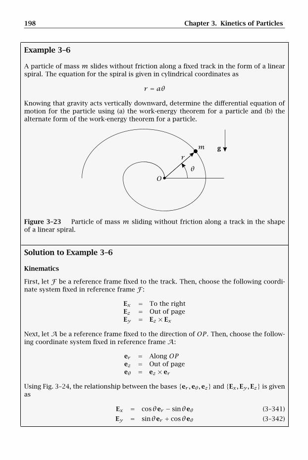
198 Chapter 3. Kinetics of Particles
Example 3–6
A particle of mass m slides without friction along a fixed track in the form of a linearspiral. The equation for the spiral is given in cylindrical coordinates as
r = aθ
Knowing that gravity acts vertically downward, determine the differential equation ofmotion for the particle using (a) the work-energy theorem for a particle and (b) thealternate form of the work-energy theorem for a particle.
gmr
Oθ
Figure 3–23 Particle of mass m sliding without friction along a track in the shapeof a linear spiral.
Solution to Example 3–6
Kinematics
First, let F be a reference frame fixed to the track. Then, choose the following coordi-nate system fixed in reference frame F :
Ex = To the rightEz = Out of pageEy = Ez × Ex
Next, let A be a reference frame fixed to the direction of OP . Then, choose the follow-ing coordinate system fixed in reference frame A:
er = Along OPez = Out of pageeθ = ez × er
Using Fig. 3–24, the relationship between the bases er ,eθ,ez and Ex,Ey,Ez is givenas
Ex = cosθer − sinθeθ (3–341)
Ey = sinθer + cosθeθ (3–342)
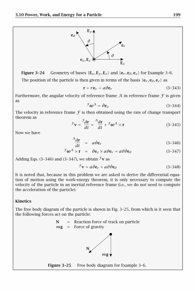
3.10 Power, Work, and Energy for a Particle 199
er
eθ
Ex
Ey
ez,Ez
θ
θ
Figure 3–24 Geometry of bases Ex,Ey,Ez and er ,eθ,ez for Example 3–6.
The position of the particle is then given in terms of the basis er ,eθ,ez as
r = rer = aθer (3–343)
Furthermore, the angular velocity of reference frame A in reference frame F is givenas
FωA = θez (3–344)
The velocity in reference frame F is then obtained using the rate of change transporttheorem as
Fv =Fdrdt
=Adrdt+ FωA × r (3–345)
Now we haveAdrdt
= aθer (3–346)
FωA × r = θez × aθer = aθθeθ (3–347)
Adding Eqs. (3–346) and (3–347), we obtain Fv as
Fv = aθer + aθθeθ (3–348)
It is noted that, because in this problem we are asked to derive the differential equa-tion of motion using the work-energy theorem, it is only necessary to compute thevelocity of the particle in an inertial reference frame (i.e., we do not need to computethe acceleration of the particle).
Kinetics
The free body diagram of the particle is shown in Fig. 3–25, from which is it seen thatthe following forces act on the particle:
N = Reaction force of track on particlemg = Force of gravity
N
mg
Figure 3–25 Free body diagram for Example 3–6.
200 Chapter 3. Kinetics of Particles
Now, because N is a contact force, we know that it must act orthogonal to the directionof the track, i.e.,
N = Nnen +Nbeb (3–349)
where en and eb are the principle unit normal and principle unit bi-normal vectors,respectively, to the track. However, because for this example the motion lies entirelyin the er ,eθ-plane, we know that the component of N in the eb-direction is zero.Consequently, the reaction force of the track reduces to
N = Nnen ≡ Nen (3–350)
As will become clear shortly, rather than obtaining an expression for N in terms of thebasis er ,eθ,ez, it is preferable to leave N in the form given in Eq. (3–350). Next, theforce of gravity is given as
mg = −mgEy (3–351)
Then, using the expression for Ey in terms of er and eθ as given in Eq. (3–342), we canwrite the force of gravity as
mg = −mg(sinθer + cosθeθ) = −mg sinθer −mg cosθeθ (3–352)
The resultant force acting on the particle is then given as
F = N+mg = Nen −mg sinθer −mg cosθeθ (3–353)
We can now proceed to use both forms of the work-energy theorem for a particle.
(a) Differential Equation Using Work-Energy Theorem
The work-energy theorem in the inertial reference frame F is given from Eq. (3–275)as
ddt
(FT
)= F · Fv (3–354)
Using the expression for Fv from Eq. (3–348), the kinetic energy in reference frame Fis given as
FT = 12m
Fv · Fv = 12m
(aθer + aθθeθ
)·(aθer + aθθeθ
)= 1
2m(a2θ2 + a2θ2θ2
)= 1
2ma2θ2(1+ θ2)
(3–355)
Computing the rate of change of FT (remembering that FT is a scalar and, thus, itsrate of change is independent of reference frame), we have
ddt
(FT
)=ma2
[θθ(1+ θ2)+ θ2(θθ)
](3–356)
Simplifying Eq. (3–356) gives
ddt
(FT
)=ma2θ
[θ(1+ θ2)+ θ2θ
](3–357)

3.10 Power, Work, and Energy for a Particle 201
Next, using the expression for F from Eq. (3–353), the power in the inertial referenceframe F produced by the resultant force F is
F · Fv = (N+mg) · Fv (3–358)
Now we know that N acts in the direction of en while Fv lies in the direction of et ,where et is tangent to the track. Therefore, we have N · Fv = 0 which implies that
F · Fv =mg · Fv = (−mg sinθer −mg cosθeθ) · (aθer + aθθeθ
)= −mga(θ sinθ + θθ cosθ)
(3–359)
Then, setting the power in Eq. (3–359) equal to the rate of change of kinetic energy asgiven in Eq. (3–357), we obtain
ma2θ[θ(1+ θ2)+ θ2θ
]= −mga(θ sinθ + θθ cosθ) (3–360)
Noting that θ ≠ 0 as a function of time (otherwise the particle would not be moving),we can drop θ from both terms in Eq. (3–360) to obtain the differential equation ofmotion as
ma2[θ(1+ θ2)+ θ2θ
]+mga(sinθ + θ cosθ) = 0 (3–361)
(b) Differential Equation Using Alternate Form of Work-Energy Theorem
The alternate form of the work-energy theorem is given in the inertial reference frameF from Eq. (3–332) as
ddt
(FE)= Fnc · Fv (3–362)
where FE is the total energy in the inertial reference frame F . Now we know that
FE = FT + FU (3–363)
where FT is the kinetic energy in the inertial reference frame F (as previously derived)while FU is the potential energy in reference frame F . Now in this problem the onlyconservative force is that due to gravity. Moreover, since gravity is a conservative force,the potential energy in reference frame F is given as
FU = FUg = −mg · r (3–364)
Substituting the expression for mg from Eq. (3–352) and the expression for r fromEq. (3–343) into (3–364), we obtain FU as
FU = − (−mg sinθer −mg cosθeθ) · aθer =mgaθ sinθ (3–365)
Then, adding FT in Eq. (3–355) to FU in Eq. (3–365), the total energy in reference frameF is obtained as
FE = FT + FU = 12ma
2θ2(1+ θ2)+mgaθ sinθ (3–366)
Computing the rate of change of FE in Eq. (3–366), we obtain
ddt
(FE)=ma2
[θθ(1+ θ2)+ θ2(θθ)
]+mga
(θ sinθ + θθ cosθ
)=ma2θ
[θ(1+ θ2)+ θ2θ
]+mgaθ (sinθ + θ cosθ)
(3–367)
202 Chapter 3. Kinetics of Particles
Finally, because N is the only nonconservative force acting on the particle and N ·Fv =0, we have
Fnc · Fv = N · Fv = 0 (3–368)
Substituting the results of Eqs. (3–367) and (3–368) into (3–362), we obtain
ma2θ[θ(1+ θ2)+ θ2θ
]+mgaθ (sinθ + θ cosθ) = 0 (3–369)
Again, noting that θ is not equal to zero as a function of time, we can drop θ fromEq. (3–369) to obtain the differential equation of motion as
ma2[θ(1+ θ2)+ θ2θ
]+mga(sinθ + θ cosθ) = 0 (3–370)
in agreement with the result from part (a) above.
Example 3–7
A collar of mass m slides without friction along a fixed horizontal rigid massless rodas shown in Fig. 3–26. The collar is attached to a linear spring with spring constantK and unstretched length 0. Knowing that q(t) is the prescribed displacement ofthe attachment point of the spring, x is the displacement of the collar relative to thespring, and assuming no gravity, determine the differential equation of motion using(a) Newton’s 2nd law and (b) the work-energy theorem for a rigid body. Also, (c) showthat an incorrect result is obtained by assuming that the spring force is conservative.
q(t)
m
x
K
PQ
Figure 3–26 Collar sliding on a fixed horizontal track attached to a linear springwith a moving attachment point.
Solution to Example 3–7
Preliminaries
The purpose of this example is to demonstrate the proper application of the linearspring force model and show that the force exerted by a linear spring with a movingattachment point is not conservative. To this end, this problem will be solved usingNewton’s 2nd law and the work-energy theorem for a particle. In addition, in order todemonstrate for this problem that the force exerted by the linear spring is not con-servative, the alternate form of the work-energy theorem will be applied using the
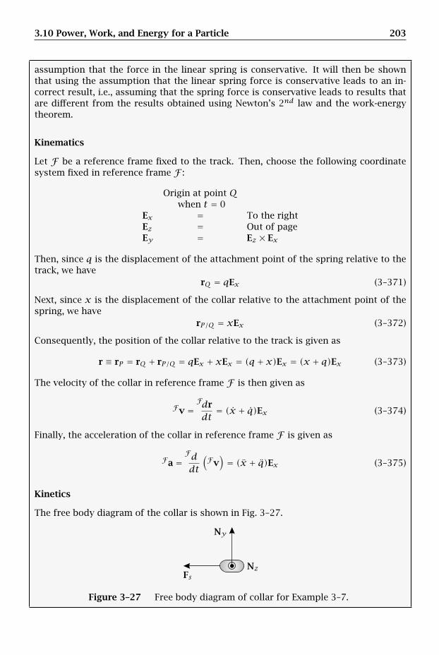
3.10 Power, Work, and Energy for a Particle 203
assumption that the force in the linear spring is conservative. It will then be shownthat using the assumption that the linear spring force is conservative leads to an in-correct result, i.e., assuming that the spring force is conservative leads to results thatare different from the results obtained using Newton’s 2nd law and the work-energytheorem.
Kinematics
Let F be a reference frame fixed to the track. Then, choose the following coordinatesystem fixed in reference frame F :
Origin at point Qwhen t = 0
Ex = To the rightEz = Out of pageEy = Ez × Ex
Then, since q is the displacement of the attachment point of the spring relative to thetrack, we have
rQ = qEx (3–371)
Next, since x is the displacement of the collar relative to the attachment point of thespring, we have
rP/Q = xEx (3–372)
Consequently, the position of the collar relative to the track is given as
r ≡ rP = rQ + rP/Q = qEx + xEx = (q + x)Ex = (x + q)Ex (3–373)
The velocity of the collar in reference frame F is then given as
Fv =Fdrdt
= (x + q)Ex (3–374)
Finally, the acceleration of the collar in reference frame F is given as
Fa =Fddt
(Fv)= (x + q)Ex (3–375)
Kinetics
The free body diagram of the collar is shown in Fig. 3–27.
Ny
NzFs
Figure 3–27 Free body diagram of collar for Example 3–7.
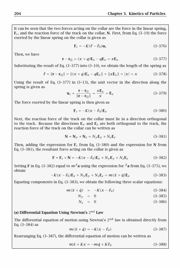
204 Chapter 3. Kinetics of Particles
It can be seen that the two forces acting on the collar are the force in the linear spring,Fs , and the reaction force of the track on the collar, N. First, from Eq. (3–19) the forceexerted by the linear spring on the collar is given as
Fs = −K( − 0)us (3–376)
Then, we haver− rQ = (x + q)Ex − qEx = xEx (3–377)
Substituting the result of Eq. (3–377) into (3–10), we obtain the length of the spring as
= ‖r− rQ‖ = ‖(x + q)Ex − qEx‖ = ‖xEx‖ = |x| = x (3–378)
Using the result of Eq. (3–377) in (3–13), the unit vector in the direction along thespring is given as
us =r− rQ‖r− rQ‖
= xExx
= Ex (3–379)
The force exerted by the linear spring is then given as
Fs = −K(x − 0)Ex (3–380)
Next, the reaction force of the track on the collar must lie in a direction orthogonalto the track. Because the directions Ey and Ez are both orthogonal to the track, thereaction force of the track on the collar can be written as
N = Ny +Nz = NyEy +NzEz (3–381)
Then, adding the expression for Fs from Eq. (3–380) and the expression for N fromEq. (3–381), the resultant force acting on the collar is given as
F = Fs +N = −K(x − 0)Ex +NyEy +NzEz (3–382)
Setting F in Eq. (3–382) equal to mFa using the expression for Fa from Eq. (3–375), weobtain
−K(x − 0)Ex +NyEy +NzEz =m(x + q)Ex (3–383)
Equating components in Eq. (3–383), we obtain the following three scalar equations:
m(x + q) = −K(x − 0) (3–384)
Ny = 0 (3–385)
Nz = 0 (3–386)
(a) Differential Equation Using Newton’s 2nd Law
The differential equation of motion using Newton’s 2nd law is obtained directly fromEq. (3–384) as
m(x + q) = −K(x − 0) (3–387)
Rearranging Eq. (3–387), the differential equation of motion can be written as
mx +Kx = −mq +K0 (3–388)
3.10 Power, Work, and Energy for a Particle 205
(b) Differential Equation Using Work-Energy Theorem
The work-energy theorem for the collar is given from Eq. (3–275) as
ddt
(FT
)= F · Fv (3–389)
First, using the velocity of the collar in reference frame F as obtained in Eq. (3–389),the kinetic energy in reference frame F is given as
FT = 12m
Fv · Fv = 12m(x + q)Ex · (x + q)Ex = 1
2m(x + q)2 (3–390)
The rate of change of FT is then given as
ddt
(FT
)=m(x + q)(x + q) (3–391)
Next, using the resultant force acting on the collar as given in Eq. (3–382), the powerproduced by all forces acting on the collar is given as
F · Fv = (Fs +N) · Fv
= (−K(x − 0)Ex +NyEy +NzEz) · (x + q)Ex= −K(x − 0)(x + q)
(3–392)
Then, setting d(FT)/dt equal to F · Fv, we obtain
m(x + q)(x + q) = −K(x − 0)(x + q) (3–393)
Rearranging Eq. (3–393) gives
(x + q) [m(x + q)+K(x − 0)] = 0 (3–394)
Now, observing that (q + x)Ex is the velocity of the collar in reference frame F , thequantity x + q cannot be equal to zero. Consequently, the term in square brackets inEq. (3–394) must be zero, i.e.,
m(x + q)+K(x − 0) = 0 (3–395)
Rearranging Eq. (3–395), we obtain
mx +Kx = −mq +K0 (3–396)
It is noted that Eq. (3–396) is identical to Eq. (3–388).
(c) Incorrect Result Obtained by Assuming Spring Force is Conservative
As discussed in Section 3.10.5, the force of a linear spring is only conservative whenthe attachment point is inertially fixed. Since in this problem it is known that theattachment point moves with velocity FvQ = qEx ≠ 0 and acceleration FaQ = qEx ≠ 0,point Q is not inertially fixed. Consequently, the force exerted by the linear spring onthe collar is not conservative.

206 Chapter 3. Kinetics of Particles
Suppose now that we assume incorrectly that the force exerted by the linear springon the collar is conservative and apply the alternate form of the work-energy theoremusing this assumption. Then, from Eq. (3–332) we would have
ddt
(FE)= Fnc · Fv (3–397)
where Fnc is the resultant nonconservative force acting on the collar. Assuming incor-rectly that the spring force is conservative, the potential energy associated with thespring force in reference frame F would be obtained from Eq. (3–296) as
FU = K2
( − 0
)2 = K2
(x − 0
)2 (3–398)
Then, using the expression for the kinetic energy from Eq. (3–390), the total energy inreference frame F would be obtained as
FE = FT + FU = 12m(x + q)2 + K
2
(x − 0
)2 (3–399)
Next, under the incorrect assumption that the spring force is conservative, the resul-tant nonconservative force acting on the collar would be given incorrectly as
Fnc = N (3–400)
which would imply
Fnc · Fv = N · Fv = (NyEy +NzEz) · (x + q)Ex = 0 (3–401)
Consequently, Eq. (3–401) simplifies to
ddt
(FE)= 0 (3–402)
Computing the rate of change of FE gives
ddt
(FE)=m(x + q)(x + q)+K(x − 0)x (3–403)
Now, unlike the result obtained using the work-energy theorem, in this case the twoterms in Eq. (3–403) do not have a common factor of x + q. Consequently, it is notpossible to set d(FE)/dt equal to zero in Eq. (3–403) and obtain the differential equa-tion of motion. Therefore, it is incorrect to assume that the force exerted by the linearspring is conservative. It is noted that, if the attachment point of the spring was iner-tially fixed, then both FvQ and FaQ would be zero, which would imply that q and qwould be zero. Then, Eq. (3–403) would reduce to
ddt
(FE)=mxx +K(x − 0)x (3–404)
Setting Eq. (3–404) equal to zero and dropping the common factor of x, we wouldobtain the correct differential equation of motion for the collar for the case where theattachment point of the spring was inertially fixed.
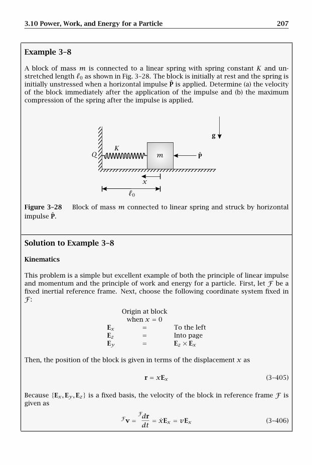
3.10 Power, Work, and Energy for a Particle 207
Example 3–8
A block of mass m is connected to a linear spring with spring constant K and un-stretched length 0 as shown in Fig. 3–28. The block is initially at rest and the spring isinitially unstressed when a horizontal impulse P is applied. Determine (a) the velocityof the block immediately after the application of the impulse and (b) the maximumcompression of the spring after the impulse is applied.
0
g
Pm
x
KQ
Figure 3–28 Block of mass m connected to linear spring and struck by horizontalimpulse P.
Solution to Example 3–8
Kinematics
This problem is a simple but excellent example of both the principle of linear impulseand momentum and the principle of work and energy for a particle. First, let F be afixed inertial reference frame. Next, choose the following coordinate system fixed inF :
Origin at blockwhen x = 0
Ex = To the leftEz = Into pageEy = Ez × Ex
Then, the position of the block is given in terms of the displacement x as
r = xEx (3–405)
Because Ex,Ey,Ez is a fixed basis, the velocity of the block in reference frame F isgiven as
Fv =Fdrdt
= xEx = vEx (3–406)

208 Chapter 3. Kinetics of Particles
Kinetics
Kinetics During Application of Impulse
The velocity of the block the instant after the impulse is applied is found by applyingthe principle of linear impulse and linear momentum of Eq. (3–179), i.e.,
F = FG(t2)− FG(t1) = FG2 − FG1 (3–407)
Now, because P is the only impulse applied to the particle, we have
F = P = PEx (3–408)
Moreover, because P is applied instantaneously, we have t1 = 0− and t2 = 0+ whichimplies that
FG1 = FG(t = 0−) = 0 (3–409)FG2 = FG(t = 0+) =mFv(t2) =mFv(t = 0+) =mv(t = 0+)Ex (3–410)
Substituting F, FG1, and FG2 from Eqs. (3–408), (3–409), and (3–410), respectively, into(3–407), we obtain
PEx =mv(t = 0+)Ex (3–411)
Solving Eq. (3–411) for v(t = 0+) gives
v(t = 0+) = Pm
(3–412)
We then obtain the velocity of the block the instant after the impulse P is applied as
Fv(t2) = Pm
Ex (3–413)
Kinetics After Application of Impulse
The maximum compression of the spring after the impulse P is applied is obtainedusing the principle of work and energy of Eq. (3–279) in reference frame F , i.e.,
FT3 − FT2 = FW23 (3–414)
The free body diagram of the block after the impulse is applied is shown in Fig. 3–29.
Fs
N
mg
Figure 3–29 Free body diagram of block in Example 3–8 after impulse P is applied.
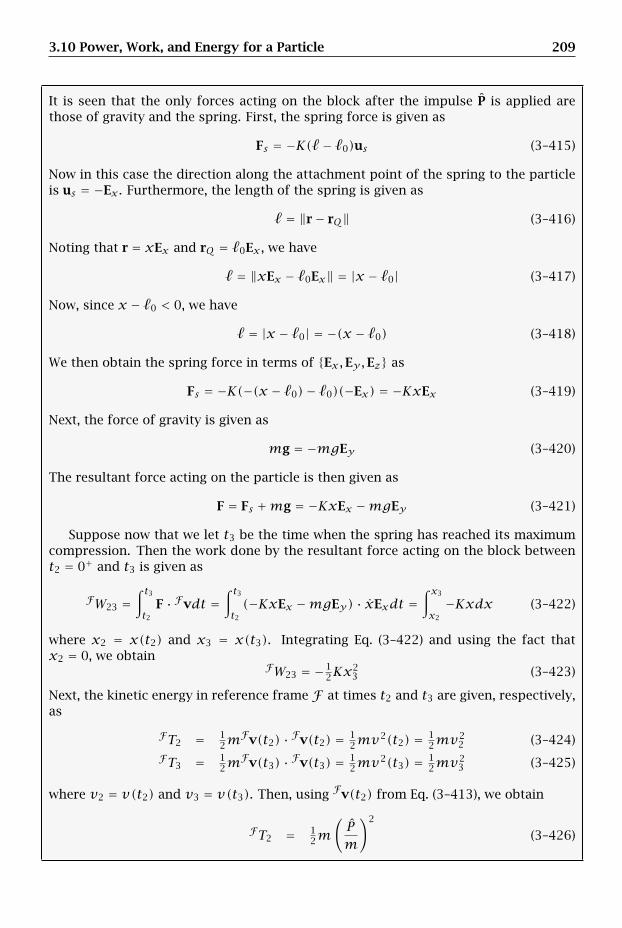
3.10 Power, Work, and Energy for a Particle 209
It is seen that the only forces acting on the block after the impulse P is applied arethose of gravity and the spring. First, the spring force is given as
Fs = −K( − 0)us (3–415)
Now in this case the direction along the attachment point of the spring to the particleis us = −Ex . Furthermore, the length of the spring is given as
= ‖r− rQ‖ (3–416)
Noting that r = xEx and rQ = 0Ex , we have
= ‖xEx − 0Ex‖ = |x − 0| (3–417)
Now, since x − 0 < 0, we have
= |x − 0| = −(x − 0) (3–418)
We then obtain the spring force in terms of Ex,Ey,Ez as
Fs = −K(−(x − 0)− 0)(−Ex) = −KxEx (3–419)
Next, the force of gravity is given as
mg = −mgEy (3–420)
The resultant force acting on the particle is then given as
F = Fs +mg = −KxEx −mgEy (3–421)
Suppose now that we let t3 be the time when the spring has reached its maximumcompression. Then the work done by the resultant force acting on the block betweent2 = 0+ and t3 is given as
FW23 =∫ t3t2
F · Fvdt =∫ t3t2(−KxEx −mgEy) · xExdt =
∫ x3
x2
−Kxdx (3–422)
where x2 = x(t2) and x3 = x(t3). Integrating Eq. (3–422) and using the fact thatx2 = 0, we obtain
FW23 = −12Kx
23 (3–423)
Next, the kinetic energy in reference frame F at times t2 and t3 are given, respectively,as
FT2 = 12m
Fv(t2) · Fv(t2) = 12mv
2(t2) = 12mv
22 (3–424)
FT3 = 12m
Fv(t3) · Fv(t3) = 12mv
2(t3) = 12mv
23 (3–425)
where v2 = v(t2) and v3 = v(t3). Then, using Fv(t2) from Eq. (3–413), we obtain
FT2 = 12m
(Pm
)2
(3–426)
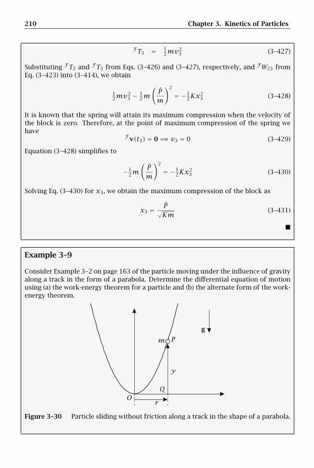
210 Chapter 3. Kinetics of Particles
FT3 = 12mv
23 (3–427)
Substituting FT2 and FT3 from Eqs. (3–426) and (3–427), respectively, and FW23 fromEq. (3–423) into (3–414), we obtain
12mv
23 − 1
2m(Pm
)2
= −12Kx
23 (3–428)
It is known that the spring will attain its maximum compression when the velocity ofthe block is zero. Therefore, at the point of maximum compression of the spring wehave
Fv(t3) = 0 ⇒ v3 = 0 (3–429)
Equation (3–428) simplifies to
−12m
(Pm
)2
= −12Kx
23 (3–430)
Solving Eq. (3–430) for x3, we obtain the maximum compression of the block as
x3 = P√Km
(3–431)
Example 3–9
Consider Example 3–2 on page 163 of the particle moving under the influence of gravityalong a track in the form of a parabola. Determine the differential equation of motionusing (a) the work-energy theorem for a particle and (b) the alternate form of the work-energy theorem.
g
m
r
y
O
P
Q
Figure 3–30 Particle sliding without friction along a track in the shape of a parabola.
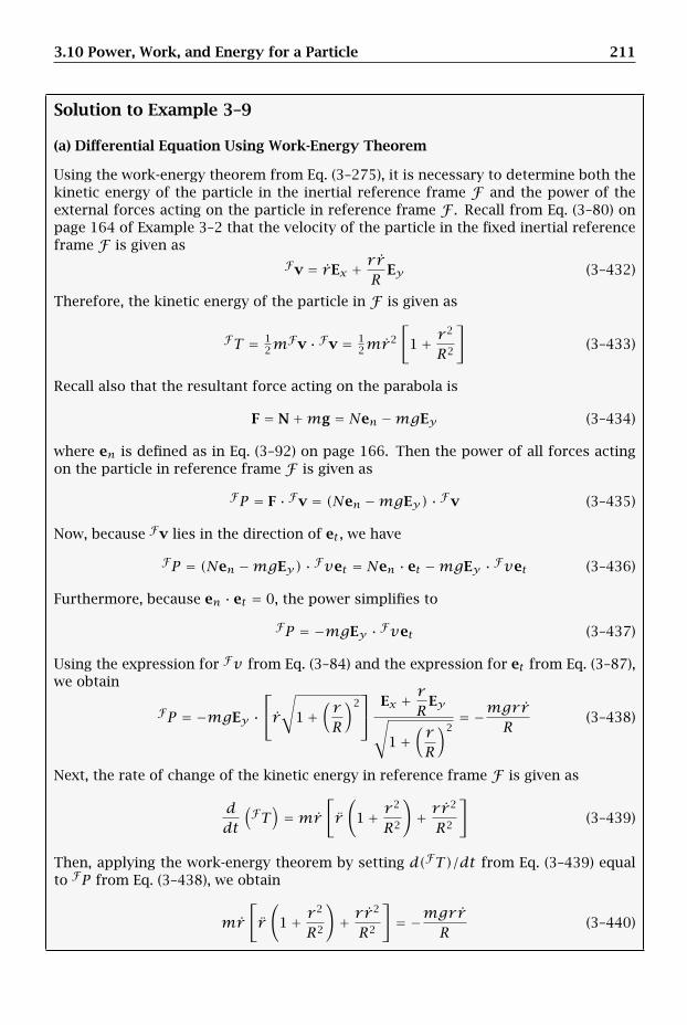
3.10 Power, Work, and Energy for a Particle 211
Solution to Example 3–9
(a) Differential Equation Using Work-Energy Theorem
Using the work-energy theorem from Eq. (3–275), it is necessary to determine both thekinetic energy of the particle in the inertial reference frame F and the power of theexternal forces acting on the particle in reference frame F . Recall from Eq. (3–80) onpage 164 of Example 3–2 that the velocity of the particle in the fixed inertial referenceframe F is given as
Fv = rEx + r rR Ey (3–432)
Therefore, the kinetic energy of the particle in F is given as
FT = 12m
Fv · Fv = 12mr
2
[1+ r
2
R2
](3–433)
Recall also that the resultant force acting on the parabola is
F = N+mg = Nen −mgEy (3–434)
where en is defined as in Eq. (3–92) on page 166. Then the power of all forces actingon the particle in reference frame F is given as
FP = F · Fv = (Nen −mgEy) · Fv (3–435)
Now, because Fv lies in the direction of et , we have
FP = (Nen −mgEy) · Fvet = Nen · et −mgEy · Fvet (3–436)
Furthermore, because en · et = 0, the power simplifies to
FP = −mgEy · Fvet (3–437)
Using the expression for Fv from Eq. (3–84) and the expression for et from Eq. (3–87),we obtain
FP = −mgEy ·⎡⎣r√
1+(rR
)2⎤⎦ Ex + rREy√
1+(rR
)2= −mgrr
R(3–438)
Next, the rate of change of the kinetic energy in reference frame F is given as
ddt
(FT
)=mr
[r(
1+ r2
R2
)+ r r
2
R2
](3–439)
Then, applying the work-energy theorem by setting d(FT)/dt from Eq. (3–439) equalto FP from Eq. (3–438), we obtain
mr[r(
1+ r2
R2
)+ r r
2
R2
]= −mgrr
R(3–440)
212 Chapter 3. Kinetics of Particles
Rearranging Eq. (3–440) gives
r(
1+ r2
R2
)+ r r
2
R2= −gr
R(3–441)
Simplifying further gives
r(
1+ r2
R2
)+ rR
(r 2
R+ g
)= 0 (3–442)
Multiplying Eq. (3–442) through by R2, we obtain
(r 2 + R2)r + r(r 2 + Rg) = 0 (3–443)
which is identical to the result obtained in Eq. (3–105) on page 167.
(b) Differential Equation Using Alternate Form of Work-Energy Theorem
In order to apply the alternate form of the work-energy theorem as given in Eq. (3–332),we need to compute the total energy in reference frame F and the power produced byall of the nonconservative forces in reference frame F . First, the kinetic energy inreference frame F is given from Eq. (3–433) of part (a). Next, it is observed that theonly two forces act on the particle are the force of gravity, mg, and the reaction forceof the track on the particle, N. First, the gravity is a constant force. Consequently, mgis conservative and its potential energy is given by Eq. (3–290) as
FUg = −mg · r (3–444)
Using the fact that mg = −mgEy , the potential energy of the force of gravity is givenas
FUg = −(−mgEy) ·(rEx + r
2
2REy
)=mg r
2
2R(3–445)
Because mg is the only conservative force acting on the particle, the total potentialenergy of the system is
FU = FUg =mg r2
2R(3–446)
The total energy of the system in reference frame F is then given as
FE = FT + FU = 12mr
2
[1+ r
2
R2
]+mg r
2
2R(3–447)
Noting that the term Fnc · Fv is accounted for by the force N, we have
Fnc · Fv = N · Fv (3–448)
But from part (a) we know that N · Fv = 0 (because N lies in the direction of en and Fvlies in the direction of et). Then, applying Eq. (3–332), we obtain
ddt
(FE)= Fnc · Fv = 0 (3–449)

3.10 Power, Work, and Energy for a Particle 213
Computing the rate of change of FE in Eq. (3–447), we obtain
ddt
(FE)=mrr
(1+ r
2
R2
)+mr 2 r r
R2+mgrr
R= 0 (3–450)
Simplifying Eq. (3–450) by dropping m and multiplying by R2, we obtain
r r(r 2 + R2
)+ r r
(r 2 + Rg
)= 0 (3–451)
Finally, dropping the common factor of r (noting that r ≠ 0 as a function of time), weobtain
r(r 2 + R2
)+ r
(r 2 + Rg
)= 0 (3–452)
which is identical to the results obtained both in part (a) and in Eq. (3–105) on page167.
Example 3–10
A particle P of mass m moves in the plane under the gravitational attraction of aparticle of mass M as shown in Fig. 3–31. Knowing that mass M is located at theinertially fixed point O, determine (a) a system of two differential equations describingthe motion of the particle, (b) the angular momentum of the particle relative to pointO,and (c) the total energy of the system. In addition, show that (d) the angular momentumof the particle is conserved in the Ez-direction and (e) the energy of the system isconserved.
m
x
y
MO
Figure 3–31 Particle of mass m moving in two dimensions under the influence of afixed mass M .
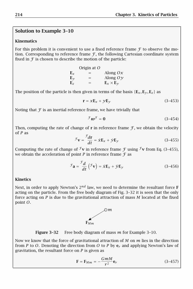
214 Chapter 3. Kinetics of Particles
Solution to Example 3–10
Kinematics
For this problem it is convenient to use a fixed reference frame F to observe the mo-tion. Corresponding to reference frame F , the following Cartesian coordinate systemfixed in F is chosen to describe the motion of the particle:
Origin at OEx = Along OxEy = Along OyEz = Ex × Ey
The position of the particle is then given in terms of the basis Ex,Ey,Ez as
r = xEx +yEy (3–453)
Noting that F is an inertial reference frame, we have trivially that
FωF = 0 (3–454)
Then, computing the rate of change of r in reference frame F , we obtain the velocityof P as
Fv =Fdrdt
= xEx + yEy (3–455)
Computing the rate of change of Fv in reference frame F using Fv from Eq. (3–455),we obtain the acceleration of point P in reference frame F as
Fa =Fddt
(Fv)= xEx + yEy (3–456)
Kinetics
Next, in order to apply Newton’s 2nd law, we need to determine the resultant force Facting on the particle. From the free body diagram of Fig. 3–32 it is seen that the onlyforce acting on P is due to the gravitational attraction of mass M located at the fixedpoint O.
FMm
m
Figure 3–32 Free body diagram of mass m for Example 3–10.
Now we know that the force of gravitational attraction of M on m lies in the directionfrom P to O. Denoting the direction from O to P by er and applying Newton’s law ofgravitation, the resultant force on P is given as
F = FMm = −GmMr 2er (3–457)
3.10 Power, Work, and Energy for a Particle 215
where r = ‖r‖ is the distance from O to P . In terms of the Cartesian coordinate systemchosen for this problem, we have
r = ‖r‖ =√x2 +y2 (3–458)
Furthermore, using the expression for r from Eq. (3–453), we have
er = rr= xEx +yEy√
x2 +y2(3–459)
Substituting r and er from Eqs. (3–458) and (3–459), respectively, into Eq. (3–457), theresultant force on m is given as
F = − GmMx2 +y2
xEx +yEy√x2 +y2
= − GmM(x2 +y2)3/2
[xEx +yEy
](3–460)
(a) System of Two Differential Equations
Applying Newton’s 2nd law to the particle by setting F from Eq. (3–460) equal to mFausing Fa from Eq. (3–456), we obtain
m[xEx + yEy
]= − GmM
(x2 +y2)3/2[xEx +yEy
](3–461)
Setting the Ex and Ey components equal yields the following two scalar equations:
mx = − GmM(x2 +y2)3/2
x (3–462)
my = − GmM(x2 +y2)3/2
y (3–463)
Rearranging Eqs. (3–462) and (3–463), we obtain the system of two differential equa-tions for mass m as
mx + GmM(x2 +y2)3/2
x = 0 (3–464)
my + GmM(x2 +y2)3/2
y = 0 (3–465)
(b) Angular Momentum of Particle Relative to Point O in Reference Frame FThe angular momentum of point P relative to point O in reference frame F is obtainedusing Eq. (3–195) as
FHO = (r− rO)×m(Fv− FvO) (3–466)
Since point O is fixed in reference frame F , we haveFvO = 0 (3–467)
Then, substituting r from Eq. (3–453) and Fv from Eq. (3–455) into (3–466), we obtain
FHO =[xEx +yEy
]×m
[xEx + yEy
](3–468)
Taking the vector products in Eq. (3–468) givesFHO =m(xy −yx)Ez (3–469)
216 Chapter 3. Kinetics of Particles
(c) Total Energy of System in Reference Frame FThe total energy of the system in reference frame F is obtained using Eq. (3–331) as
FE = FT + FU (3–470)
First, using the expression for Fv from Eq. (3–455), the kinetic energy of point P inreference frame F is obtained using Eq. (3–271) on page 189 as
FT+ = 12m
Fv · Fv = 12m[x2 + y2
](3–471)
Next, for this problem, the only force acting on the particle is the conservative force ofgravitational attraction of M on m. Using the expression for the potential energy dueto gravitational attraction from Eq. (3–310), we obtain the potential energy in referenceframe F as
FU = FUg = −GmMr = − GmM√x2 +y2
(3–472)
where r =√x2 +y2 from Eq. (3–458) has been used in Eq. (3–472). Then, using the
kinetic energy in reference frame F from Eq. (3–471) and the potential energy in refer-ence frame F from Eq. (3–472), the total energy of the system in reference frame F isobtained from Eq. (3–470) as
FE = 12m[x2 + y2
]− GmM√
x2 +y2(3–473)
(d) Conservation of Angular Momentum of Particle in Ez-Direction
In accordance with Eq. (3–215), in order to show that the angular momentum aboutpoint O in the Ez-direction is conserved, we must show that
(MO − (r− rO)×mFaO
)· Ez + FHO ·
FdEzdt
= 0 (3–474)
Now, since O is fixed in the inertial reference frame F , it follows that FaO = 0. Further-more, since Ez is fixed in reference frame F , we have that d(FEz)/dt = 0. Therefore,we must show that
MO · Ez = 0 (3–475)
So we then need to show that MO ·Ez is zero. Since rO = 0, we have the moment of theresultant force on P relative to point O as
MO = r× F (3–476)
Using r from Eq. (3–453) and F from Eq. (3–460), we obtain MO as
MO =[xEx +yEy
]×[− GmM(x2 +y2)3/2
(xEx +yEy
)](3–477)
Computing the vector products in Eq. (3–477), we obtain
MO = − GmM(x2 +y2)3/2
xyEz + GmM(x2 +y2)3/2
xyEz = 0 (3–478)
3.10 Power, Work, and Energy for a Particle 217
Then, because MO = 0, we have trivially that
MO · Ez = 0 (3–479)
Consequently, we have shown that the quantity in Eq. (3–474) is zero and, hence, thatangular momentum in the Ez-direction is conserved.
(e) Conservation of Energy
In order to show that energy is conserved, we need to show that the rate of change ofFE is zero. Differentiating the total energy from Eq. (3–473), we have
ddt
(FE)=mxx +myy + 1
2GmM
(x2 +y2)3/2(2xx + 2yy) (3–480)
Rearranging Eq. (3–480) gives
ddt
(FE)= x
[mx + GmM
(x2 +y2)3/2x]+ y
[my + GmM
(x2 +y2)3/2y]
(3–481)
Then, substituting the results of Eqs. (3–464) and (3–465) into Eq. (3–481), we obtain
ddt
(FE)= x [0]+ y [0] = 0 (3–482)
Equation (3–482) implies that the total energy of the particle in reference frame F isconserved.
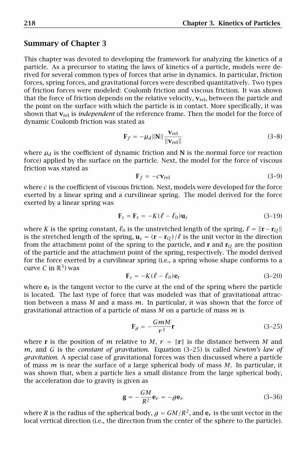
218 Chapter 3. Kinetics of Particles
Summary of Chapter 3
This chapter was devoted to developing the framework for analyzing the kinetics of aparticle. As a precursor to stating the laws of kinetics of a particle, models were de-rived for several common types of forces that arise in dynamics. In particular, frictionforces, spring forces, and gravitational forces were described quantitatively. Two typesof friction forces were modeled: Coulomb friction and viscous friction. It was shownthat the force of friction depends on the relative velocity, vrel, between the particle andthe point on the surface with which the particle is in contact. More specifically, it wasshown that vrel is independent of the reference frame. Then the model for the force ofdynamic Coulomb friction was stated as
Ff = −µd‖N‖vrel
‖vrel‖(3–8)
where µd is the coefficient of dynamic friction and N is the normal force (or reactionforce) applied by the surface on the particle. Next, the model for the force of viscousfriction was stated as
Ff = −cvrel (3–9)
where c is the coefficient of viscous friction. Next, models were developed for the forceexerted by a linear spring and a curvilinear spring. The model derived for the forceexerted by a linear spring was
Fs = Fs = −K( − 0)us (3–19)
where K is the spring constant, 0 is the unstretched length of the spring, = ‖r− rQ‖is the stretched length of the spring, us = (r− rQ)/ is the unit vector in the directionfrom the attachment point of the spring to the particle, and r and rQ are the positionof the particle and the attachment point of the spring, respectively. The model derivedfor the force exerted by a curvilinear spring (i.e., a spring whose shape conforms to acurve C in R3) was
Fs = −K( − 0)et (3–20)
where et is the tangent vector to the curve at the end of the spring where the particleis located. The last type of force that was modeled was that of gravitational attrac-tion between a mass M and a mass m. In particular, it was shown that the force ofgravitational attraction of a particle of mass M on a particle of mass m is
Fg = −GmMr 3r (3–25)
where r is the position of m relative to M , r = ‖r‖ is the distance between M andm, and G is the constant of gravitation. Equation (3–25) is called Newton’s law ofgravitation. A special case of gravitational forces was then discussed where a particleof mass m is near the surface of a large spherical body of mass M . In particular, itwas shown that, when a particle lies a small distance from the large spherical body,the acceleration due to gravity is given as
g = −GMR2
er = −ger (3–36)
where R is the radius of the spherical body, g = GM/R2, and er is the unit vector in thelocal vertical direction (i.e., the direction from the center of the sphere to the particle).
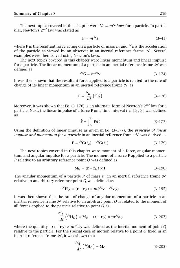
Summary of Chapter 3 219
The next topics covered in this chapter were Newton’s laws for a particle. In partic-ular, Newton’s 2nd law was stated as
F =mNa (3–41)
where F is the resultant force acting on a particle of massm and Na is the accelerationof the particle as viewed by an observer in an inertial reference frame N . Severalexamples were then solved using Newton’s laws.
The next topics covered in this chapter were linear momentum and linear impulsefor a particle. The linear momentum of a particle in an inertial reference frame N wasdefined as
NG =mNv (3–174)
It was then shown that the resultant force applied to a particle is related to the rate ofchange of its linear momentum in an inertial reference frame N as
F =Nddt
(NG
)(3–176)
Moreover, it was shown that Eq. (3–176) is an alternate form of Newton’s 2nd law for aparticle. Next, the linear impulse of a force F on a time interval t ∈ [t1, t2] was definedas
F =∫ t2t1
Fdt (3–177)
Using the definition of linear impulse as given in Eq. (3–177), the principle of linearimpulse and momentum for a particle in an inertial reference frame N was derived as
F = NG(t2)−NG(t1) (3–179)
The next topics covered in this chapter were moment of a force, angular momen-tum, and angular impulse for a particle. The moment of a force F applied to a particleP relative to an arbitrary reference point Q was defined as
MQ = (r− rQ)× F (3–190)
The angular momentum of a particle P of mass m in an inertial reference frame Nrelative to an arbitrary reference point Q was defined as
NHQ = (r− rQ)×m(Nv−NvQ) (3–195)
It was then shown that the rate of change of angular momentum of a particle in aninertial reference frame N relative to an arbitrary point Q is related to the moment ofall forces applied to the particle relative to point Q as
Nddt
(NHQ
)= MQ − (r− rQ)×mNaQ (3–203)
where the quantity −(r − rQ) ×mNaQ was defined as the inertial moment of point Qrelative to the particle. For the special case of motion relative to a point O fixed in aninertial reference frame N , it was shown that
Nddt
(NHO
)= MO (3–205)
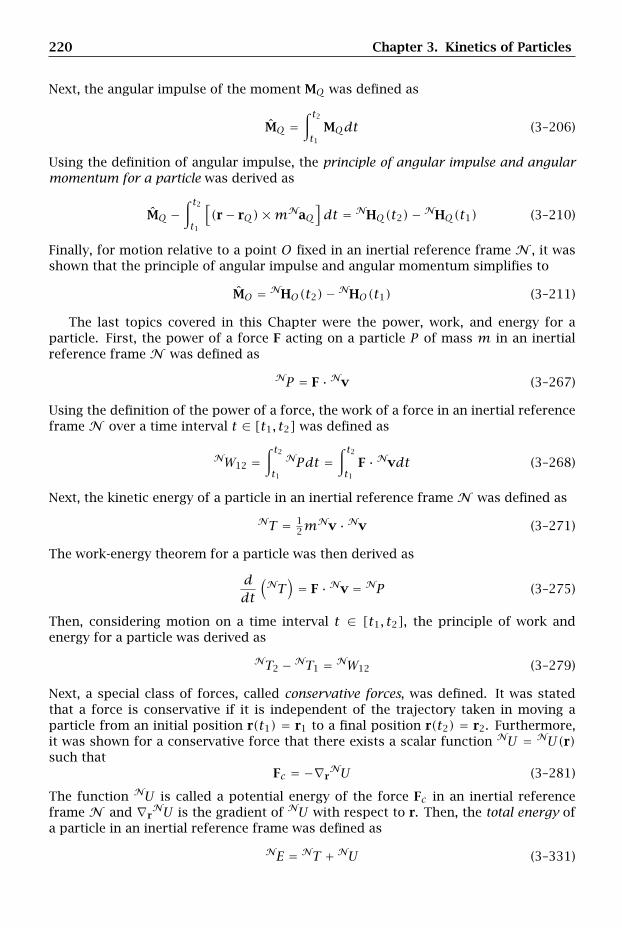
220 Chapter 3. Kinetics of Particles
Next, the angular impulse of the moment MQ was defined as
MQ =∫ t2t1
MQdt (3–206)
Using the definition of angular impulse, the principle of angular impulse and angularmomentum for a particle was derived as
MQ −∫ t2t1
[(r− rQ)×mNaQ
]dt = NHQ(t2)−NHQ(t1) (3–210)
Finally, for motion relative to a point O fixed in an inertial reference frame N , it wasshown that the principle of angular impulse and angular momentum simplifies to
MO = NHO(t2)−NHO(t1) (3–211)
The last topics covered in this Chapter were the power, work, and energy for aparticle. First, the power of a force F acting on a particle P of mass m in an inertialreference frame N was defined as
NP = F · Nv (3–267)
Using the definition of the power of a force, the work of a force in an inertial referenceframe N over a time interval t ∈ [t1, t2] was defined as
NW12 =∫ t2t1
NPdt =∫ t2t1
F · Nvdt (3–268)
Next, the kinetic energy of a particle in an inertial reference frame N was defined as
NT = 12m
Nv · Nv (3–271)
The work-energy theorem for a particle was then derived as
ddt
(NT
)= F · Nv = NP (3–275)
Then, considering motion on a time interval t ∈ [t1, t2], the principle of work andenergy for a particle was derived as
NT2 −NT1 = NW12 (3–279)
Next, a special class of forces, called conservative forces, was defined. It was statedthat a force is conservative if it is independent of the trajectory taken in moving aparticle from an initial position r(t1) = r1 to a final position r(t2) = r2. Furthermore,it was shown for a conservative force that there exists a scalar function NU = NU(r)such that
Fc = −∇rNU (3–281)
The function NU is called a potential energy of the force Fc in an inertial referenceframe N and ∇r
NU is the gradient of NU with respect to r. Then, the total energy ofa particle in an inertial reference frame was defined as
NE = NT +NU (3–331)
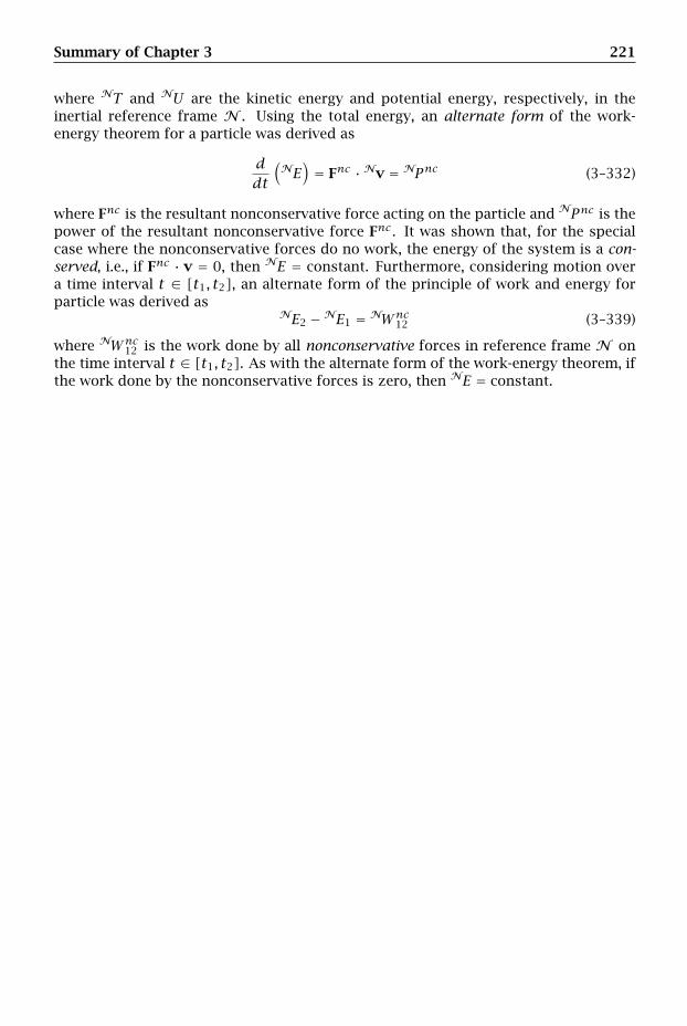
Summary of Chapter 3 221
where NT and NU are the kinetic energy and potential energy, respectively, in theinertial reference frame N . Using the total energy, an alternate form of the work-energy theorem for a particle was derived as
ddt
(NE
)= Fnc · Nv = NPnc (3–332)
where Fnc is the resultant nonconservative force acting on the particle and NPnc is thepower of the resultant nonconservative force Fnc . It was shown that, for the specialcase where the nonconservative forces do no work, the energy of the system is a con-served, i.e., if Fnc · v = 0, then NE = constant. Furthermore, considering motion overa time interval t ∈ [t1, t2], an alternate form of the principle of work and energy forparticle was derived as
NE2 −NE1 = NWnc12 (3–339)
where NWnc12 is the work done by all nonconservative forces in reference frame N on
the time interval t ∈ [t1, t2]. As with the alternate form of the work-energy theorem, ifthe work done by the nonconservative forces is zero, then NE = constant.

222 Chapter 3. Kinetics of Particles
Problems for Chapter 3
3.1 A particle of mass m moves in the vertical plane along a track in the form of acircle as shown in Fig. P3-1. The equation for the track is
r = r0 cosθ
Knowing that gravity acts downward and assuming the initial conditions θ(t = 0) = 0and θ(t = 0) = θ0, determine (a) the differential equation of motion for the particleand (b) the force exerted by the track on the particle as a function of θ.
r =r0
cosθgm
Oθ
Figure P3-1
3.2 A collar of mass m slides without friction along a rigid massless rod as shownin Fig. P3-2. The collar is attached to a linear spring with spring constant K and un-stretched length L. Assuming no gravity, determine the differential equation of motionfor the collar.
m
x
KL
O
Figure P3-2
3.3 A bead of mass m slides along a fixed circular helix of radius R and constanthelical inclination angle φ as shown in Fig. P3-3. The equation for the helix is given incylindrical coordinates as
z = Rθ tanφ
Knowing that gravity acts vertically downward, determine the differential equationof motion for the bead in terms of the angle θ using (a) Newton’s 2nd law and (b)
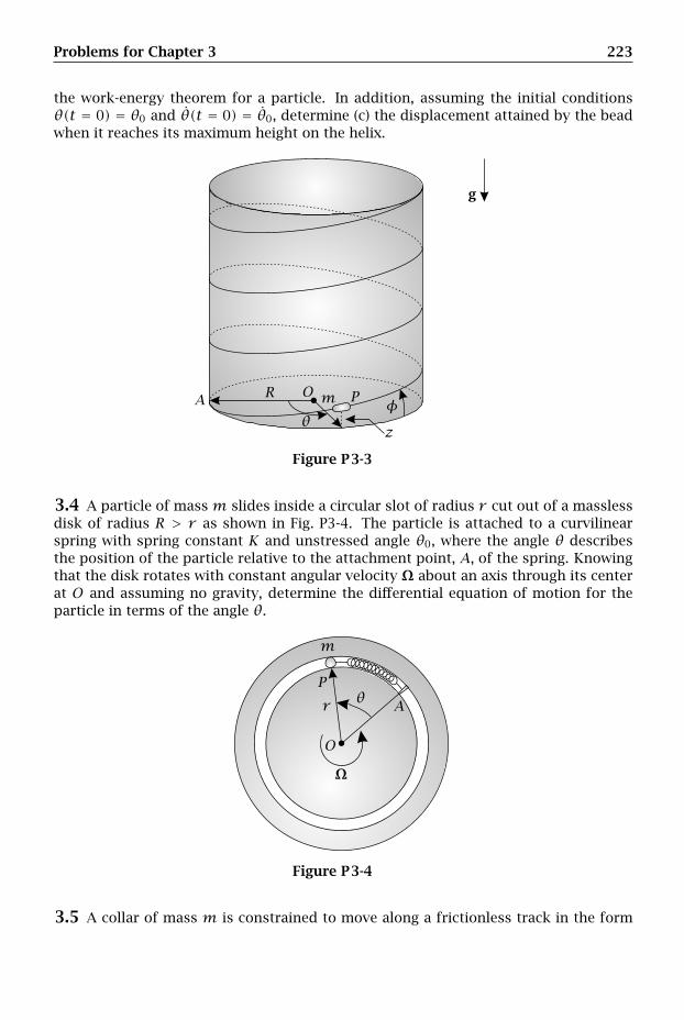
Problems for Chapter 3 223
the work-energy theorem for a particle. In addition, assuming the initial conditionsθ(t = 0) = θ0 and θ(t = 0) = θ0, determine (c) the displacement attained by the beadwhen it reaches its maximum height on the helix.
g
m
z
A O PR
θφ
Figure P3-3
3.4 A particle of massm slides inside a circular slot of radius r cut out of a masslessdisk of radius R > r as shown in Fig. P3-4. The particle is attached to a curvilinearspring with spring constant K and unstressed angle θ0, where the angle θ describesthe position of the particle relative to the attachment point, A, of the spring. Knowingthat the disk rotates with constant angular velocity Ω about an axis through its centerat O and assuming no gravity, determine the differential equation of motion for theparticle in terms of the angle θ.
m
r A
O
Pθ
Ω
Figure P3-4
3.5 A collar of mass m is constrained to move along a frictionless track in the form

224 Chapter 3. Kinetics of Particles
of a logarithmic spiral as shown in Fig. P3-5. The equation for the spiral is given as
r = r0e−aθ
where r0 and a are constants and θ is the angle as shown in the figure. Assuming thatgravity acts downward, determine the differential equation of motion in terms of theangle θ using (a) Newton’s 2nd law and (b) the work-energy theorem for a particle.
r= r
0e−aθg
m
Oθ
Figure P3-5
3.6 A block of mass m is initially at rest atop a frictionless horizontal surface whenit is struck by a horizontal impulse P as shown in Fig. P3-6. After the impulse isapplied, the block slides along the surface until it reaches a frictionless circular trackof radius r . Knowing that gravity acts downward, determine (a) the velocity of theblock immediately after the application of the impulse P and (b) the magnitude of theimpulse P for which the block is moving with zero velocity as it reaches the top of thetrack.
Circular Track
g
P m
r
Figure P3-6
3.7 A particle of massm slides without friction along the inner surface of a fixed coneof semi-vertex angle β as shown in the Fig. P3-7. The equation for the cone is given incylindrical coordinates as
z = r cotβ
Knowing that the basis Ex,Ey,Ez is fixed to the cone; θ is the angle between theEx-direction and the direction OQ, where Q is the projection of the particle into the
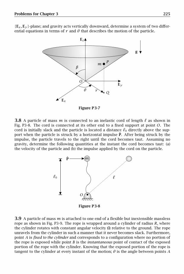
Problems for Chapter 3 225
Ex,Ey-plane; and gravity acts vertically downward, determine a system of two differ-ential equations in terms of r and θ that describes the motion of the particle.
Ex
Ey
Ez
g
m
r
O
P
Q
β
θ
Figure P3-7
3.8 A particle of mass m is connected to an inelastic cord of length as shown inFig. P3-8. The cord is connected at its other end to a fixed support at point O. Thecord is initially slack and the particle is located a distance 0 directly above the sup-port when the particle is struck by a horizontal impulse P. After being struck by theimpulse, the particle travels to the right until the cord becomes taut. Assuming nogravity, determine the following quantities at the instant the cord becomes taut: (a)the velocity of the particle and (b) the impulse applied by the cord on the particle.
0
P m
O
Figure P3-8
3.9 A particle of massm is attached to one end of a flexible but inextensible masslessrope as shown in Fig. P3-9. The rope is wrapped around a cylinder of radius R, wherethe cylinder rotates with constant angular velocity Ω relative to the ground. The ropeunravels from the cylinder in such a manner that it never becomes slack. Furthermore,point A is fixed to the cylinder and corresponds to a configuration where no portion ofthe rope is exposed while point B is the instantaneous point of contact of the exposedportion of the rope with the cylinder. Knowing that the exposed portion of the rope istangent to the cylinder at every instant of the motion; θ is the angle between points A

226 Chapter 3. Kinetics of Particles
and B; and assuming the initial conditions θ(t = 0) = 0, θ(t = 0) = Ω (where Ω = ‖Ω‖),determine (a) the differential equation for the particle in terms of the variable θ, and(b) the tension in the rope as a function of time.
m
A
B
O
P
R
θ
Ω
Figure P3-9
3.10 A particle of mass m moves under the influence of gravity in the vertical planealong a track as shown in Fig. P3-10. The equation for the track is given in Cartesiancoordinates as
y = − ln cosx
where −π/2 < x < π/2. Using the horizontal component of position, x, as the variableto describe the motion, determine the differential equation of motion for the particleusing (a) Newton’s 2nd law and (b) one of the forms of the work-energy theorem for aparticle.
y = − ln cosx
Ex
Ey
g m
O
Figure P3-10
3.11 A particle of mass m moves in the horizontal plane as shown in Fig. P3-11. Theparticle is attached to a linear spring with spring constant K and unstretched length while the spring is attached at its other end to the fixed point O. Assuming no gravity,(a) determine a system of two differential equations of motion for the particle in termsof the variables r and θ, (b) show that the total energy of the system is conserved, and(c) show that the angular momentum relative to point O is conserved.
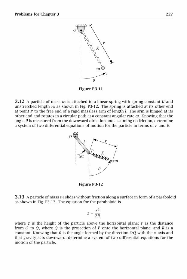
Problems for Chapter 3 227
m
rK
O
θ
Figure P3-11
3.12 A particle of mass m is attached to a linear spring with spring constant K andunstretched length r0 as shown in Fig. P3-12. The spring is attached at its other endat point P to the free end of a rigid massless arm of length l. The arm is hinged at itsother end and rotates in a circular path at a constant angular rateω. Knowing that theangle θ is measured from the downward direction and assuming no friction, determinea system of two differential equations of motion for the particle in terms of r and θ.
ωt
l
m
r
K
O
P
θ
Figure P3-12
3.13 A particle of massm slides without friction along a surface in form of a paraboloidas shown in Fig. P3-13. The equation for the paraboloid is
z = r2
2R
where z is the height of the particle above the horizontal plane; r is the distancefrom O to Q, where Q is the projection of P onto the horizontal plane; and R is aconstant. Knowing that θ is the angle formed by the direction OQ with the x-axis andthat gravity acts downward, determine a system of two differential equations for themotion of the particle.

228 Chapter 3. Kinetics of Particles
z = r2
2R
g
m
r
x
y
z
O
P
Qθ
Figure P3-13
3.14 A particle of mass m slides without friction along the inside of a fixed hemi-spherical bowl of radius R as shown in Fig. P3-14. Furthermore, the angle θ is mea-sured from the Ex-direction to the direction OQ, where point Q lies on the rim of thebowl while the angle φ is measured from the OQ-direction to the position of the par-ticle. Knowing that gravity acts downward, (a) determine a system of two differentialequations in terms of the angles θ and φ that describes the motion of the particle, (b)show that the angular momentum about the Ez-direction is conserved, and (c) showthat the total energy of the system is conserved.
Ex
Ey
Ez
g
m
O
Q
R
θφ
Figure P3-14
3.15 A massless disk of radius R rolls without slip at a constant angular rateω alonga horizontal surface as shown in Fig. P3-15. A particle of massm slides without frictionin a slot cut along a radial direction of the disk. Attached to the particle is a linearspring with spring constant K, unstretched length r0, and attachment point O, where
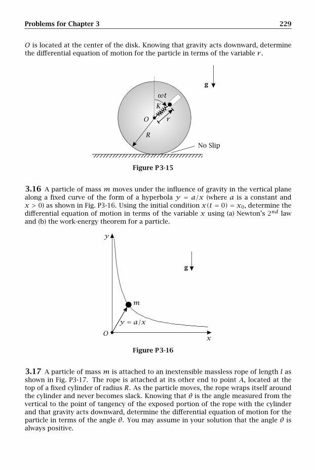
Problems for Chapter 3 229
O is located at the center of the disk. Knowing that gravity acts downward, determinethe differential equation of motion for the particle in terms of the variable r .
ωt
No Slip
g
r
K
O
R
Figure P3-15
3.16 A particle of mass m moves under the influence of gravity in the vertical planealong a fixed curve of the form of a hyperbola y = a/x (where a is a constant andx > 0) as shown in Fig. P3-16. Using the initial condition x(t = 0) = x0, determine thedifferential equation of motion in terms of the variable x using (a) Newton’s 2nd lawand (b) the work-energy theorem for a particle.
y = a/x
g
m
x
y
O
Figure P3-16
3.17 A particle of mass m is attached to an inextensible massless rope of length l asshown in Fig. P3-17. The rope is attached at its other end to point A, located at thetop of a fixed cylinder of radius R. As the particle moves, the rope wraps itself aroundthe cylinder and never becomes slack. Knowing that θ is the angle measured from thevertical to the point of tangency of the exposed portion of the rope with the cylinderand that gravity acts downward, determine the differential equation of motion for theparticle in terms of the angle θ. You may assume in your solution that the angle θ isalways positive.
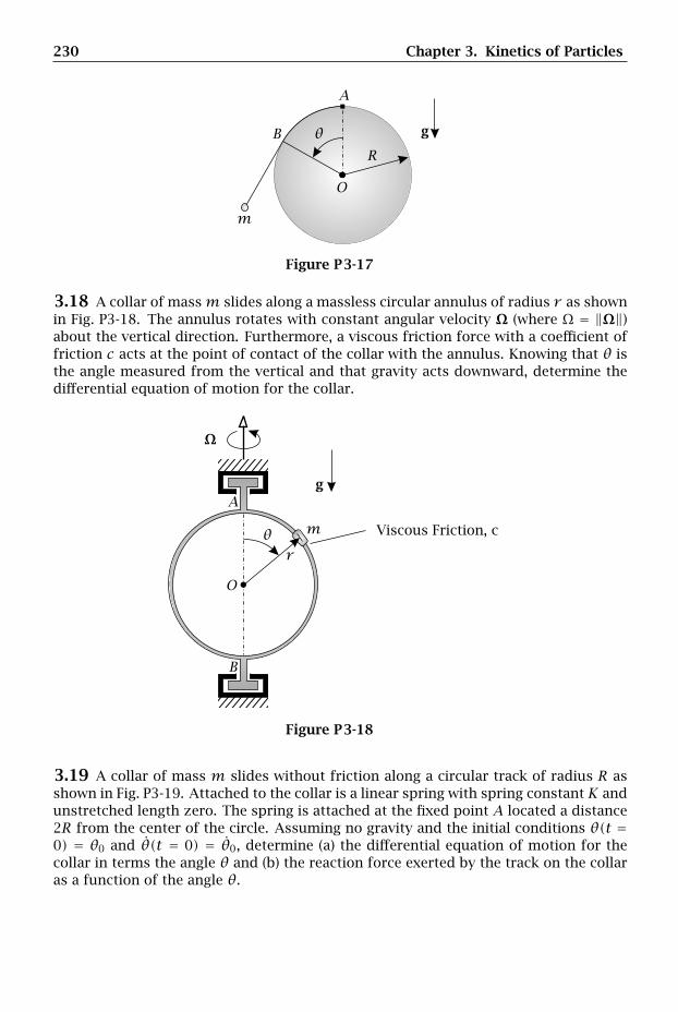
230 Chapter 3. Kinetics of Particles
g
m
A
B
O
Rθ
Figure P3-17
3.18 A collar of massm slides along a massless circular annulus of radius r as shownin Fig. P3-18. The annulus rotates with constant angular velocity Ω (where Ω = ‖Ω‖)about the vertical direction. Furthermore, a viscous friction force with a coefficient offriction c acts at the point of contact of the collar with the annulus. Knowing that θ isthe angle measured from the vertical and that gravity acts downward, determine thedifferential equation of motion for the collar.
Viscous Friction, c
g
m
r
A
B
O
θ
Ω
Figure P3-18
3.19 A collar of mass m slides without friction along a circular track of radius R asshown in Fig. P3-19. Attached to the collar is a linear spring with spring constant K andunstretched length zero. The spring is attached at the fixed point A located a distance2R from the center of the circle. Assuming no gravity and the initial conditions θ(t =0) = θ0 and θ(t = 0) = θ0, determine (a) the differential equation of motion for thecollar in terms the angle θ and (b) the reaction force exerted by the track on the collaras a function of the angle θ.
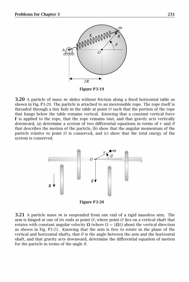
Problems for Chapter 3 231
m
A
K
O
R
2R
θ
Figure P3-19
3.20 A particle of mass m slides without friction along a fixed horizontal table asshown in Fig. P3-20. The particle is attached to an inextensible rope. The rope itself isthreaded through a tiny hole in the table at point O such that the portion of the ropethat hangs below the table remains vertical. Knowing that a constant vertical forceF is applied to the rope, that the rope remains taut, and that gravity acts verticallydownward, (a) determine a system of two differential equations in terms of r and θthat describes the motion of the particle, (b) show that the angular momentum of theparticle relative to point O is conserved, and (c) show that the total energy of thesystem is conserved.
Fg
mr
Oθ
Figure P3-20
3.21 A particle mass m is suspended from one end of a rigid massless arm. Thearm is hinged at one of its ends at point O, where point O lies on a vertical shaft thatrotates with constant angular velocity Ω (where Ω = ‖Ω‖) about the vertical directionas shown in Fig. P3-21. Knowing that the arm is free to rotate in the plane of thevertical and horizontal shafts, that θ is the angle between the arm and the horizontalshaft, and that gravity acts downward, determine the differential equation of motionfor the particle in terms of the angle θ.
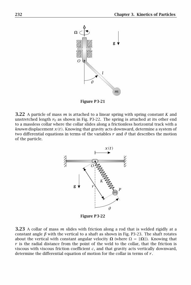
232 Chapter 3. Kinetics of Particles
g
l
m
O
θ
Ω
Figure P3-21
3.22 A particle of mass m is attached to a linear spring with spring constant K andunstretched length r0 as shown in Fig. P3-22. The spring is attached at its other endto a massless collar where the collar slides along a frictionless horizontal track with aknown displacement x(t). Knowing that gravity acts downward, determine a system oftwo differential equations in terms of the variables r and θ that describes the motionof the particle.
x(t)
g
mr
K
O
P
θ
Figure P3-22
3.23 A collar of mass m slides with friction along a rod that is welded rigidly at aconstant angle β with the vertical to a shaft as shown in Fig. P3-23. The shaft rotatesabout the vertical with constant angular velocity Ω (where Ω = ‖Ω‖). Knowing thatr is the radial distance from the point of the weld to the collar, that the friction isviscous with viscous friction coefficient c, and that gravity acts vertically downward,determine the differential equation of motion for the collar in terms of r .

Problems for Chapter 3 233
Viscous Friction, c
g
mr
O
P
β
Ω
Figure P3-23
3.24 A particle of massm slides without friction along a track in the form of a spiralas shown in Fig. P3-24. The equation for the spiral is
r = aθ
where a is a constant and θ is the angle measured from the horizontal. Assuming nogravity, determine the differential equation of motion for the particle in terms of theangle θ using (a) Newton’s 2nd law and (b) the work-energy theorem for a particle.
mr
Oθ
Figure P3-24
3.25 A particle of mass m slides without friction along a track in the form of aparabola as shown in Fig. P3-25. The equation for the parabola is
y = r2
2a
where a is a constant, r is the distance from point O to point Q, point Q is the pro-jection of the particle onto the horizontal direction, and y is the vertical distance.Furthermore, the particle is attached to a linear spring with spring constant K and un-stretched length x0. The spring is always aligned horizontally such that its attachmentpoint is free to slide along a vertical shaft through the center of the parabola. Knowingthat the parabola rotates with constant angular velocity Ω (where Ω = ‖Ω‖) about the
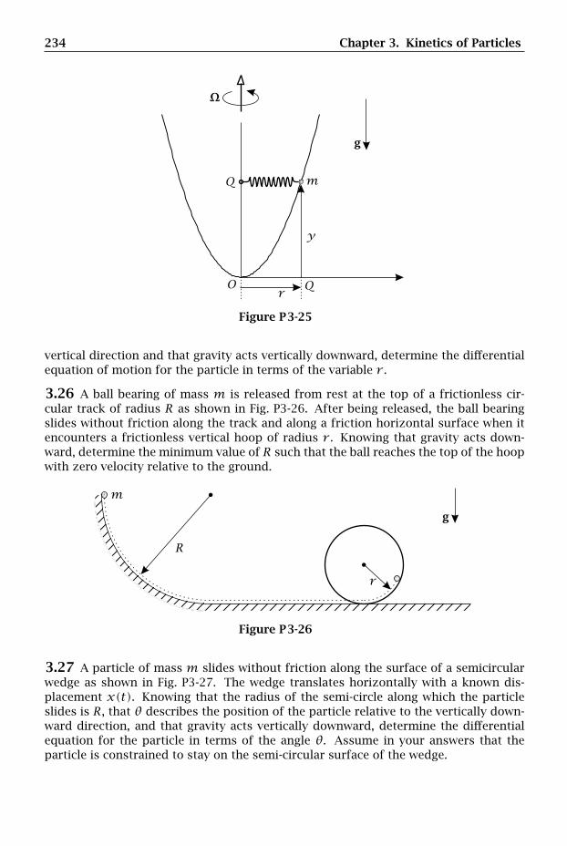
234 Chapter 3. Kinetics of Particles
g
m
r
y
O
Q
Q
Ω
Figure P3-25
vertical direction and that gravity acts vertically downward, determine the differentialequation of motion for the particle in terms of the variable r .
3.26 A ball bearing of mass m is released from rest at the top of a frictionless cir-cular track of radius R as shown in Fig. P3-26. After being released, the ball bearingslides without friction along the track and along a friction horizontal surface when itencounters a frictionless vertical hoop of radius r . Knowing that gravity acts down-ward, determine the minimum value of R such that the ball reaches the top of the hoopwith zero velocity relative to the ground.
g
m
r
R
Figure P3-26
3.27 A particle of mass m slides without friction along the surface of a semicircularwedge as shown in Fig. P3-27. The wedge translates horizontally with a known dis-placement x(t). Knowing that the radius of the semi-circle along which the particleslides is R, that θ describes the position of the particle relative to the vertically down-ward direction, and that gravity acts vertically downward, determine the differentialequation for the particle in terms of the angle θ. Assume in your answers that theparticle is constrained to stay on the semi-circular surface of the wedge.
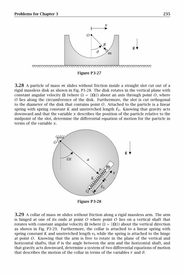
Problems for Chapter 3 235
g
m
x
O
R
θ
Figure P3-27
3.28 A particle of mass m slides without friction inside a straight slot cut out of arigid massless disk as shown in Fig. P3-28. The disk rotates in the vertical plane withconstant angular velocity Ω (where Ω = ‖Ω‖) about an axis through point O, whereO lies along the circumference of the disk. Furthermore, the slot is cut orthogonalto the diameter of the disk that contains point O. Attached to the particle is a linearspring with spring constant K and unstretched length 0. Knowing that gravity actsdownward and that the variable x describes the position of the particle relative to themidpoint of the slot, determine the differential equation of motion for the particle interms of the variable x.
0
Ωt
g
a
mx
K
O
P
Q
Figure P3-28
3.29 A collar of mass m slides without friction along a rigid massless arm. The armis hinged at one of its ends at point O where point O lies on a vertical shaft thatrotates with constant angular velocity Ω (where Ω = ‖Ω‖) about the vertical directionas shown in Fig. P3-29. Furthermore, the collar is attached to a linear spring withspring constant K and unstretched length r0 while the spring is attached to the hingeat point O. Knowing that the arm is free to rotate in the plane of the vertical andhorizontal shafts, that θ is the angle between the arm and the horizontal shaft, andthat gravity acts downward, determine a system of two differential equations of motionthat describes the motion of the collar in terms of the variables r and θ.
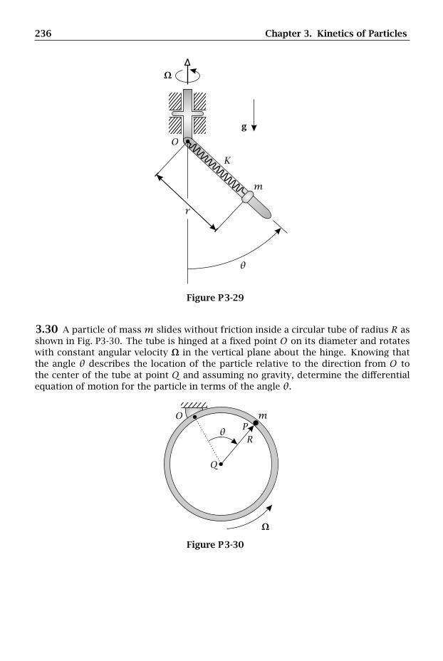
236 Chapter 3. Kinetics of Particles
g
m
r
K
O
θ
Ω
Figure P3-29
3.30 A particle of massm slides without friction inside a circular tube of radius R asshown in Fig. P3-30. The tube is hinged at a fixed point O on its diameter and rotateswith constant angular velocity Ω in the vertical plane about the hinge. Knowing thatthe angle θ describes the location of the particle relative to the direction from O tothe center of the tube at point Q and assuming no gravity, determine the differentialequation of motion for the particle in terms of the angle θ.
mOP
Q
Rθ
Ω
Figure P3-30
Chapter 4
Kinetics of a System of Particles
The most incomprehensible thing about the world is that it is at all compre-hensible.
- Albert Einstein (1879–1955)German and American Physicist
In Chapter 3 we discussed the important principles and methods used in the for-mulation, solution, and analysis of the motion of a single particle. In this chapter weextend the results of particle kinetics to systems consisting of two or more particles.
The first topic covered in this chapter is the center of mass of a system of parti-cles. Using the definition of the center of mass, the linear momentum of a system ofparticles is defined. Then, using the definition of linear momentum, the velocity andacceleration of the center of mass of the system are defined.
The second topic covered in this chapter is the angular momentum of a system ofparticles. In particular, expressions for the angular momentum are derived relative toan arbitrary point, an inertially fixed point, and the center of mass of the system. Then,relationships between these three different forms of angular momentum are derived.
The third and fourth topics covered in this chapter are Newton’s 2nd law and therate of change of angular momentum for a system of particles. In particular, it is shownthat the center of mass of the system satisfies Newton’s 2nd law. Furthermore, the keyresults relating the rate of change of angular momentum for a system of particles tomoment applied to the system are derived.
The fifth topic covered in this chapter is impulse and momentum for a system ofparticles. First, using Newton’s 2nd law for a system of particles, the principle of linearimpulse and linear momentum for a system of particles is derived. Then, using theresults from the rate of change of the angular momentum for a system of particles,the principle of angular impulse and angular momentum for a system of particles isderived.
The sixth topic covered in this chapter is work and energy for a system of parti-cles. First, the kinetic energy for a system of particles is defined. Then, an alternateexpression for the kinetic energy, called Koenig’s decomposition, is derived. Using thekinetic energy, the work-energy theorem for a system of particles is derived. Then,
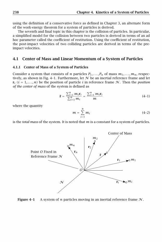
238 Chapter 4. Kinetics of a System of Particles
using the definition of a conservative force as defined in Chapter 3, an alternate formof the work-energy theorem for a system of particles is derived.
The seventh and final topic in this chapter is the collision of particles. In particular,a simplified model for the collision between two particles is derived in terms of an adhoc parameter called the coefficient of restitution. Using the coefficient of restitution,the post-impact velocities of two colliding particles are derived in terms of the pre-impact velocities.
4.1 Center of Mass and Linear Momentum of a System of Particles
4.1.1 Center of Mass of a System of Particles
Consider a system that consists of n particles P1, . . . , Pn of mass m1, . . . ,mn, respec-tively, as shown in Fig. 4–1. Furthermore, let N be an inertial reference frame and letri (i = 1, . . . , n) be the position of particle i in reference frame N . Then the positionof the center of mass of the system is defined as
r =∑ni=1miri∑ni=1mi
=∑ni=1mirim
(4–1)
where the quantity
m =n∑i=1
mi (4–2)
is the total mass of the system. It is noted thatm is a constant for a system of particles.
Point O Fixed in
N
Reference Frame N
Center of Mass
ri
rnr
r1
r2
m1
m2
mi
mn
O
Figure 4–1 A system of n particles moving in an inertial reference frame N .
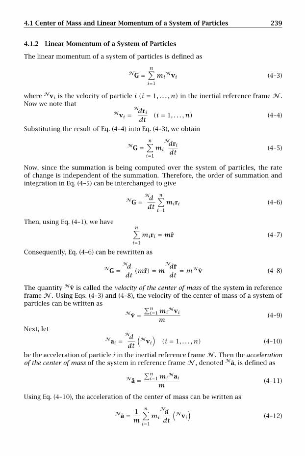
4.1 Center of Mass and Linear Momentum of a System of Particles 239
4.1.2 Linear Momentum of a System of Particles
The linear momentum of a system of particles is defined as
NG =n∑i=1
miNvi (4–3)
where Nvi is the velocity of particle i (i = 1, . . . , n) in the inertial reference frame N .Now we note that
Nvi =Ndridt
(i = 1, . . . , n) (4–4)
Substituting the result of Eq. (4–4) into Eq. (4–3), we obtain
NG =n∑i=1
mi
Ndridt
(4–5)
Now, since the summation is being computed over the system of particles, the rateof change is independent of the summation. Therefore, the order of summation andintegration in Eq. (4–5) can be interchanged to give
NG =Nddt
n∑i=1
miri (4–6)
Then, using Eq. (4–1), we haven∑i=1
miri =mr (4–7)
Consequently, Eq. (4–6) can be rewritten as
NG =Nddt(mr) =m
Ndrdt
=mNv (4–8)
The quantity Nv is called the velocity of the center of mass of the system in referenceframe N . Using Eqs. (4–3) and (4–8), the velocity of the center of mass of a system ofparticles can be written as
Nv =∑ni=1mi
Nvim
(4–9)
Next, let
Nai =Nddt
(Nvi
)(i = 1, . . . , n) (4–10)
be the acceleration of particle i in the inertial reference frameN . Then the accelerationof the center of mass of the system in reference frame N , denoted Na, is defined as
Na =∑ni=1mi
Naim
(4–11)
Using Eq. (4–10), the acceleration of the center of mass can be written as
Na = 1m
n∑i=1
mi
Nddt
(Nvi
)(4–12)
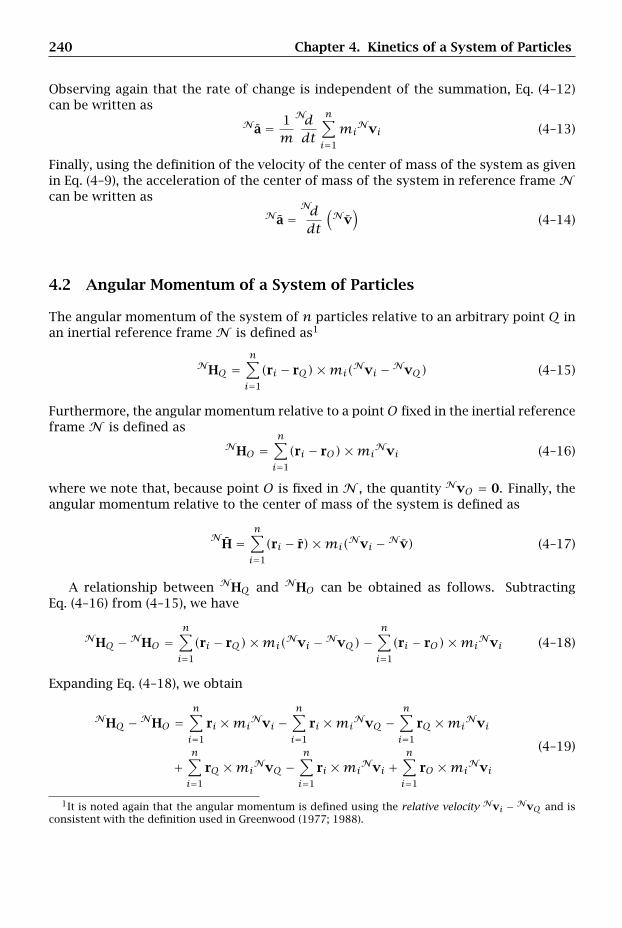
240 Chapter 4. Kinetics of a System of Particles
Observing again that the rate of change is independent of the summation, Eq. (4–12)can be written as
Na = 1m
Nddt
n∑i=1
miNvi (4–13)
Finally, using the definition of the velocity of the center of mass of the system as givenin Eq. (4–9), the acceleration of the center of mass of the system in reference frame Ncan be written as
Na =Nddt
(Nv
)(4–14)
4.2 Angular Momentum of a System of Particles
The angular momentum of the system of n particles relative to an arbitrary point Q inan inertial reference frame N is defined as1
NHQ =n∑i=1
(ri − rQ)×mi(Nvi −NvQ) (4–15)
Furthermore, the angular momentum relative to a pointO fixed in the inertial referenceframe N is defined as
NHO =n∑i=1
(ri − rO)×miNvi (4–16)
where we note that, because point O is fixed in N , the quantity NvO = 0. Finally, theangular momentum relative to the center of mass of the system is defined as
NH =
n∑i=1
(ri − r)×mi(Nvi −Nv) (4–17)
A relationship between NHQ and NHO can be obtained as follows. SubtractingEq. (4–16) from (4–15), we have
NHQ −NHO =n∑i=1
(ri − rQ)×mi(Nvi −NvQ)−n∑i=1
(ri − rO)×miNvi (4–18)
Expanding Eq. (4–18), we obtain
NHQ −NHO =n∑i=1
ri ×miNvi −
n∑i=1
ri ×miNvQ −
n∑i=1
rQ ×miNvi
+n∑i=1
rQ ×miNvQ −
n∑i=1
ri ×miNvi +
n∑i=1
rO ×miNvi
(4–19)
1It is noted again that the angular momentum is defined using the relative velocity Nvi −NvQ and isconsistent with the definition used in Greenwood (1977; 1988).
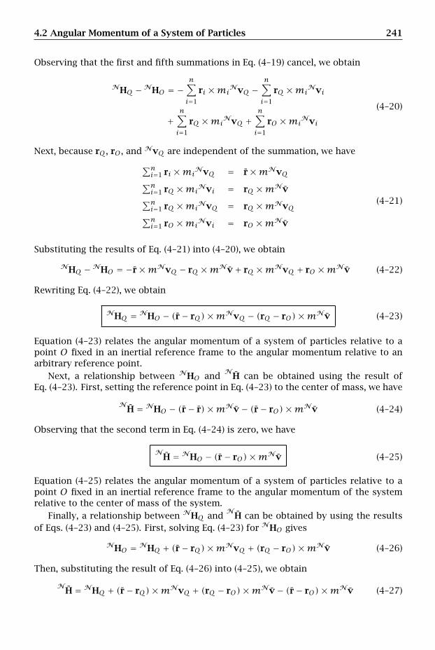
4.2 Angular Momentum of a System of Particles 241
Observing that the first and fifth summations in Eq. (4–19) cancel, we obtain
NHQ −NHO = −n∑i=1
ri ×miNvQ −
n∑i=1
rQ ×miNvi
+n∑i=1
rQ ×miNvQ +
n∑i=1
rO ×miNvi
(4–20)
Next, because rQ, rO , and NvQ are independent of the summation, we have
∑ni=1 ri ×mi
NvQ = r×mNvQ∑ni=1 rQ ×mi
Nvi = rQ ×mNv∑ni=1 rQ ×mi
NvQ = rQ ×mNvQ∑ni=1 rO ×mi
Nvi = rO ×mNv
(4–21)
Substituting the results of Eq. (4–21) into (4–20), we obtain
NHQ −NHO = −r×mNvQ − rQ ×mNv+ rQ ×mNvQ + rO ×mNv (4–22)
Rewriting Eq. (4–22), we obtain
NHQ = NHO − (r− rQ)×mNvQ − (rQ − rO)×mNv (4–23)
Equation (4–23) relates the angular momentum of a system of particles relative to apoint O fixed in an inertial reference frame to the angular momentum relative to anarbitrary reference point.
Next, a relationship between NHO andN
H can be obtained using the result ofEq. (4–23). First, setting the reference point in Eq. (4–23) to the center of mass, we have
NH = NHO − (r− r)×mNv− (r− rO)×mNv (4–24)
Observing that the second term in Eq. (4–24) is zero, we have
NH = NHO − (r− rO)×mNv (4–25)
Equation (4–25) relates the angular momentum of a system of particles relative to apoint O fixed in an inertial reference frame to the angular momentum of the systemrelative to the center of mass of the system.
Finally, a relationship between NHQ andN
H can be obtained by using the resultsof Eqs. (4–23) and (4–25). First, solving Eq. (4–23) for NHO gives
NHO = NHQ + (r− rQ)×mNvQ + (rQ − rO)×mNv (4–26)
Then, substituting the result of Eq. (4–26) into (4–25), we obtain
NH = NHQ + (r− rQ)×mNvQ + (rQ − rO)×mNv− (r− rO)×mNv (4–27)
242 Chapter 4. Kinetics of a System of Particles
Rearranging and simplifying Eq. (4–27), we obtain
NHQ = NH+ (rQ − r)×m(NvQ −Nv) (4–28)
Equation (4–28) relates the angular momentum of a system of particles relative toan arbitrary point Q to the angular momentum relative to the center of mass of thesystem.
4.3 Newton’s 2nd Law for a System of Particles
Suppose now that we let Ri be the resultant force acting on particle i in a system of nparticles. The resultant force acting on particle i can be decomposed into two parts:(1) a force that is external to the system and (2) a force due to all of the other particlesin the system. For convenience, let
Fi = Force exerted on particle i external to systemfij = Force exerted on particle i by particle j (j = 1, . . . , n)
(i = 1, . . . , n)
Now from Newton’s 3rd law we know that the force exerted by particle i on particle jis equal and opposite the force exerted by particle j on particle i. Consequently,
fji = −fij (i, j = 1, . . . , n) (4–29)
Furthermore, because a particle cannot exert a force on itself, we have
fii = 0 (i = 1, . . . , n) (4–30)
In addition, it is assumed that the force exerted by particle j on particle i lies alongthe line between particle i and particle j.2 Consequently, the resultant force acting onparticle i, denoted Ri, is given as
Ri = Fi +n∑j=1
fij (i = 1,2, . . . , n) (4–31)
Then, applying Newton’s 2nd law to particle i, we have
Ri =miNai (i = 1,2, . . . , n) (4–32)
Substituting Eq. (4–31) into (4–32), we obtain
Fi +n∑j=1
fij =miNai (i = 1,2, . . . , n) (4–33)
Next, summing forces over all particles in the system, we obtain
n∑i=1
⎡⎣Fi +
n∑j=1
fij
⎤⎦ = n∑
i=1
Fi +n∑i=1
n∑j=1
fij =n∑i=1
miNai (4–34)
2The assumption that fij lies along the line between particles i and j is commonly referred to as the
strong form of Newton’s 3rd law (Thornton and Marion, 2004).
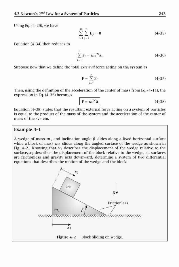
4.3 Newton’s 2nd Law for a System of Particles 243
Using Eq. (4–29), we haven∑i=1
n∑j=1
fij = 0 (4–35)
Equation (4–34) then reduces to
n∑i=1
Fi =miNai (4–36)
Suppose now that we define the total external force acting on the system as
F =n∑i=1
Fi (4–37)
Then, using the definition of the acceleration of the center of mass from Eq. (4–11), theexpression in Eq. (4–36) becomes
F =mNa (4–38)
Equation (4–38) states that the resultant external force acting on a system of particlesis equal to the product of the mass of the system and the acceleration of the center ofmass of the system.
Example 4–1
A wedge of mass m1 and inclination angle β slides along a fixed horizontal surfacewhile a block of mass m2 slides along the angled surface of the wedge as shown inFig. 4–2. Knowing that x1 describes the displacement of the wedge relative to thesurface, x2 describes the displacement of the block relative to the wedge, all surfacesare frictionless and gravity acts downward, determine a system of two differentialequations that describes the motion of the wedge and the block.
Frictionless
g
m1
m2
x1
x2
β
Figure 4–2 Block sliding on wedge.
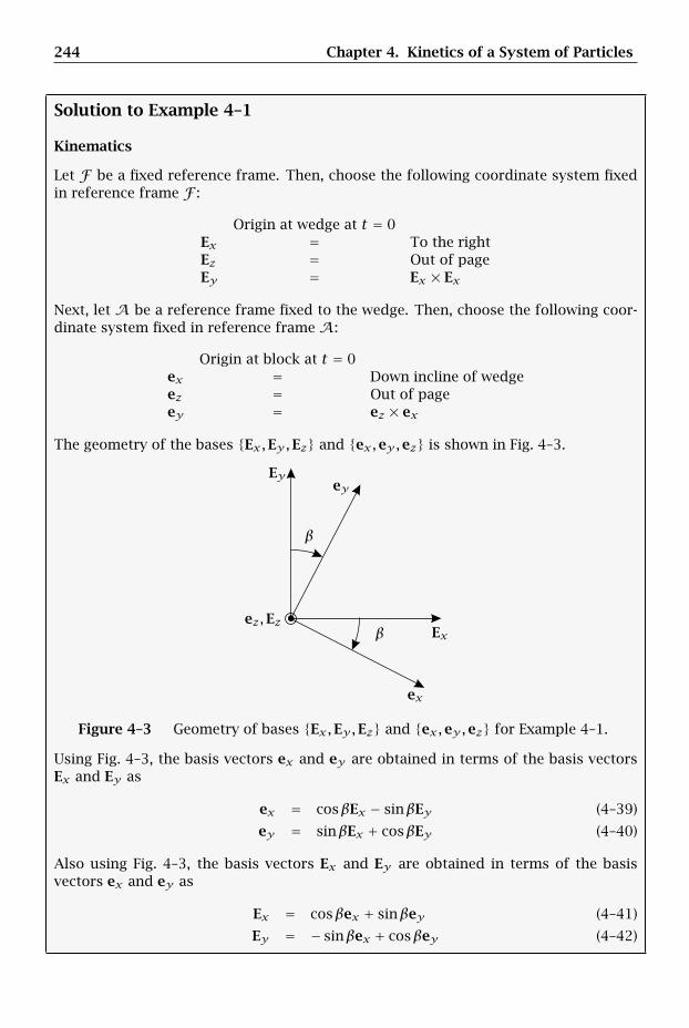
244 Chapter 4. Kinetics of a System of Particles
Solution to Example 4–1
Kinematics
Let F be a fixed reference frame. Then, choose the following coordinate system fixedin reference frame F :
Origin at wedge at t = 0Ex = To the rightEz = Out of pageEy = Ex × Ex
Next, let A be a reference frame fixed to the wedge. Then, choose the following coor-dinate system fixed in reference frame A:
Origin at block at t = 0ex = Down incline of wedgeez = Out of pageey = ez × ex
The geometry of the bases Ex,Ey,Ez and ex,ey,ez is shown in Fig. 4–3.
ex
ey
Ex
Ey
ez,Ez
β
β
Figure 4–3 Geometry of bases Ex,Ey,Ez and ex,ey,ez for Example 4–1.
Using Fig. 4–3, the basis vectors ex and ey are obtained in terms of the basis vectorsEx and Ey as
ex = cosβEx − sinβEy (4–39)
ey = sinβEx + cosβEy (4–40)
Also using Fig. 4–3, the basis vectors Ex and Ey are obtained in terms of the basisvectors ex and ey as
Ex = cosβex + sinβey (4–41)
Ey = − sinβex + cosβey (4–42)
4.3 Newton’s 2nd Law for a System of Particles 245
Kinematics of Wedge
In terms of the basis ex,ey,Ez, the position of the wedge is given as
r1 = x1Ex (4–43)
Then, the velocity of the wedge in reference frame F is given as
Fv1 =Fdr1
dt= x1Ex (4–44)
Finally, the acceleration of the wedge in reference frame F is obtained as
Fa1 =Fddt
(Fv1
)= x1Ex (4–45)
Kinematics of Block
The position of the block is given as
r2 = r1 + r2/1 (4–46)
where r1 and r2/1 are the position of the wedge and the position of the block relativeto the wedge, respectively. Now, because the block slides along the wedge, we have
r2/1 = x2ex (4–47)
Substituting the expression for r1 from Eq. (4–43) and the expression for r2/1 fromEq. (4–47) into Eq. (4–46), we obtain the position of the block as
r2 = x1Ex + x2ex (4–48)
Differentiating the position of the block as given in Eq. (4–48) in reference frame F(observing that the bases Ex,Ey,Ez and ex,ey,ez do not rotate), we obtain thevelocity of the block in reference frame F as
Fv2 =Fdr2
dt= x1Ex + x2ex (4–49)
Furthermore, differentiating Fv2 as given in Eq. (4–49) in reference frame F , we obtainthe acceleration of the block in reference frame F as
Fa2 =Fddt
(Fv2
)= x1Ex + x2ex (4–50)
Kinematics of Center of Mass of System
The acceleration of the center of mass of the wedge-block system is given as
Fa = m1Fa1 +m2
Fa2
m1 +m2(4–51)
Substituting the expressions for Fa1 and Fa2 from Eqs. (4–45) and (4–50), respectively,the acceleration of the center of mass in reference frame F is obtained as
Fa = m1x1Ex +m2(x1Ex + x2ex)m1 +m2
= x1Ex + m2
m1 +m2x2ex (4–52)
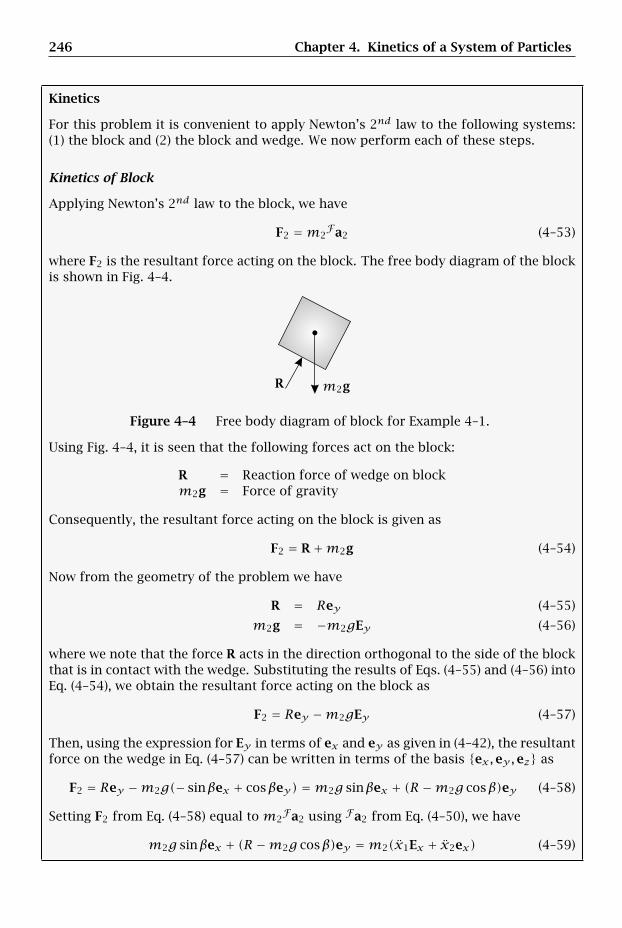
246 Chapter 4. Kinetics of a System of Particles
Kinetics
For this problem it is convenient to apply Newton’s 2nd law to the following systems:(1) the block and (2) the block and wedge. We now perform each of these steps.
Kinetics of Block
Applying Newton’s 2nd law to the block, we have
F2 =m2Fa2 (4–53)
where F2 is the resultant force acting on the block. The free body diagram of the blockis shown in Fig. 4–4.
R m2g
Figure 4–4 Free body diagram of block for Example 4–1.
Using Fig. 4–4, it is seen that the following forces act on the block:
R = Reaction force of wedge on blockm2g = Force of gravity
Consequently, the resultant force acting on the block is given as
F2 = R+m2g (4–54)
Now from the geometry of the problem we have
R = Rey (4–55)
m2g = −m2gEy (4–56)
where we note that the force R acts in the direction orthogonal to the side of the blockthat is in contact with the wedge. Substituting the results of Eqs. (4–55) and (4–56) intoEq. (4–54), we obtain the resultant force acting on the block as
F2 = Rey −m2gEy (4–57)
Then, using the expression for Ey in terms of ex and ey as given in (4–42), the resultantforce on the wedge in Eq. (4–57) can be written in terms of the basis ex,ey,ez as
F2 = Rey −m2g(− sinβex + cosβey) =m2g sinβex + (R −m2g cosβ)ey (4–58)
Setting F2 from Eq. (4–58) equal to m2Fa2 using Fa2 from Eq. (4–50), we have
m2g sinβex + (R −m2g cosβ)ey =m2(x1Ex + x2ex) (4–59)
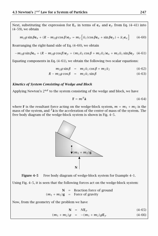
4.3 Newton’s 2nd Law for a System of Particles 247
Next, substituting the expression for Ex in terms of ex and ey from Eq. (4–41) into(4–59), we obtain
m2g sinβex + (R −m2g cosβ)ey =m2
[x1(cosβex + sinβey)+ x2ex
](4–60)
Rearranging the right-hand side of Eq. (4–60), we obtain
−m2g sinβex + (R −m2g cosβ)ey = (m2x1 cosβ+m2x2)ex +m2x1 sinβey (4–61)
Equating components in Eq. (4–61), we obtain the following two scalar equations:
m2g sinβ = m2x1 cosβ+m2x2 (4–62)
R −m2g cosβ = m2x1 sinβ (4–63)
Kinetics of System Consisting of Wedge and Block
Applying Newton’s 2nd to the system consisting of the wedge and block, we have
F =mFa (4–64)
where F is the resultant force acting on the wedge-block system, m =m1 +m2 is themass of the system, and Fa is the acceleration of the center of mass of the system. Thefree body diagram of the wedge-block system is shown in Fig. 4–5.
N
(m1 +m2)g
Figure 4–5 Free body diagram of wedge-block system for Example 4–1.
Using Fig. 4–5, it is seen that the following forces act on the wedge-block system:
N = Reaction force of ground(m1 +m2)g = Force of gravity
Now, from the geometry of the problem we have
N = NEy (4–65)
(m1 +m2)g = −(m1 +m2)gEy (4–66)
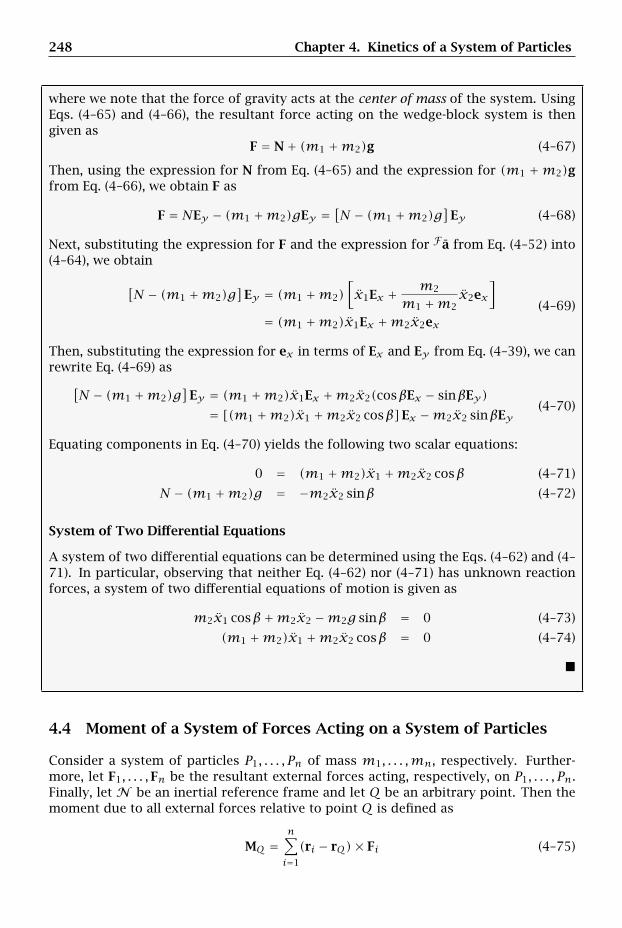
248 Chapter 4. Kinetics of a System of Particles
where we note that the force of gravity acts at the center of mass of the system. UsingEqs. (4–65) and (4–66), the resultant force acting on the wedge-block system is thengiven as
F = N+ (m1 +m2)g (4–67)
Then, using the expression for N from Eq. (4–65) and the expression for (m1 +m2)gfrom Eq. (4–66), we obtain F as
F = NEy − (m1 +m2)gEy =[N − (m1 +m2)g
]Ey (4–68)
Next, substituting the expression for F and the expression for Fa from Eq. (4–52) into(4–64), we obtain
[N − (m1 +m2)g
]Ey = (m1 +m2)
[x1Ex + m2
m1 +m2x2ex
]
= (m1 +m2)x1Ex +m2x2ex(4–69)
Then, substituting the expression for ex in terms of Ex and Ey from Eq. (4–39), we canrewrite Eq. (4–69) as
[N − (m1 +m2)g
]Ey = (m1 +m2)x1Ex +m2x2(cosβEx − sinβEy)= [(m1 +m2)x1 +m2x2 cosβ]Ex −m2x2 sinβEy
(4–70)
Equating components in Eq. (4–70) yields the following two scalar equations:
0 = (m1 +m2)x1 +m2x2 cosβ (4–71)
N − (m1 +m2)g = −m2x2 sinβ (4–72)
System of Two Differential Equations
A system of two differential equations can be determined using the Eqs. (4–62) and (4–71). In particular, observing that neither Eq. (4–62) nor (4–71) has unknown reactionforces, a system of two differential equations of motion is given as
m2x1 cosβ+m2x2 −m2g sinβ = 0 (4–73)
(m1 +m2)x1 +m2x2 cosβ = 0 (4–74)
4.4 Moment of a System of Forces Acting on a System of Particles
Consider a system of particles P1, . . . , Pn of mass m1, . . . ,mn, respectively. Further-more, let F1, . . . ,Fn be the resultant external forces acting, respectively, on P1, . . . , Pn.Finally, let N be an inertial reference frame and let Q be an arbitrary point. Then themoment due to all external forces relative to point Q is defined as
MQ =n∑i=1
(ri − rQ)× Fi (4–75)

4.5 Rate of Change of Angular Momentum for a System of Particles 249
Next, the moment due to all external forces relative to a point O fixed in the inertialreference frame N is defined as
MO =n∑i=1
(ri − rO)× Fi (4–76)
Finally, the moment due to all external forces relative to the center of mass of thesystem is defined as
M =n∑i=1
(ri − r)× Fi (4–77)
4.5 Rate of Change of Angular Momentum for a System of Particles
Suppose that we compute the rate of change of NHQ in Eq. (4–15). We then obtain
Nddt
(NHQ
)=
n∑i=1
(Nvi −NvQ)×mi(Nvi −NvQ)
+n∑i=1
(ri − rQ)×mi(Nai −NaQ)
(4–78)
We note thatn∑i=1
(Nvi −NvQ)×mi(Nvi −NvQ) = 0
Consequently, Eq. (4–78) reduces to
Nddt
(NHQ
)=
n∑i=1
(ri − rQ)×mi(Nai −NaQ) (4–79)
Equation (4–79) can be rewritten as
Nddt
(NHQ
)=
n∑i=1
(ri − rQ)×miNai −
n∑i=1
(ri − rQ)×miNaQ (4–80)
Separating the second summation in Eq. (4–80), we obtain
Nddt
(NHQ
)=
n∑i=1
(ri − rQ)×miNai −
n∑i=1
ri ×miNaQ +
n∑i=1
rQ ×miNaQ (4–81)
Then, applying the results of Eqs. (4–2), (4–1), and (4–11) and observing that rQ andNaQ are independent of the summation, we have
Nddt
(NHQ
)=
n∑i=1
(ri − rQ)×miNai − (r− rQ)×mNaQ (4–82)
Substituting Eq. (4–33) into (4–82) gives
Nddt
(NHQ
)=
n∑i=1
(ri − rQ)×⎡⎣Fi +
n∑j=1
fij
⎤⎦− (r− rQ)×mNaQ (4–83)

250 Chapter 4. Kinetics of a System of Particles
Separating the first summation of Eq. (4–83), we obtain
Nddt
(NHQ
)=
n∑i=1
(ri − rQ)× Fi +n∑i=1
n∑j=1
(ri − rQ)× fij − (r− rQ)×mNaQ (4–84)
Then, from the assumption that the forces fij (i, j = 1,2, . . . , n) satisfy the strong formof Newton’s 3rd law, we have
n∑i=1
n∑j=1
(ri − rQ)× fij = 0 (4–85)
Consequently, Eq. (4–84) reduces to
Nddt
(NHQ
)=
n∑i=1
(ri − rQ)× Fi − (r− rQ)×mNaQ (4–86)
Then, using the definition of the moment of a force for a system of particles relativeto an arbitrary point Q as given in Eq. (4–75), Eq. (4–86) becomes
MQ − (r− rQ)×mNaQ =Nddt
(NHQ
)(4–87)
Equation (4–87) relates the rate of change of the angular momentum of a system ofparticles relative to an arbitrary reference point Q to the resultant moment due to allexternal forces applied relative to Q. Similar to Eq. (3–204) on page 180 for a singleparticle, the quantity
−(r− rQ)×mNaQ (4–88)
is called the inertial moment of the reference point Q relative to the center of mass ofthe system.
Now consider motion relative to a reference point O, where O is fixed in an inertialreference frameN . In this case the acceleration of point O is zero, i.e., NaQ = 0, whichimplies that −(r − rQ) ×mNaQ = 0. Then, substituting the expression for MO givenin Eq. (4–76) for the moment due to all external forces relative to a point fixed in aninertial reference frame, Eq. (4–87) becomes
MO =Nddt
(NHO
)(4–89)
Next, consider motion relative to the center of mass of the system. Because the ref-erence point is the center of mass, we have r − rQ = 0, which again implies that−(r − r) ×mNaQ = 0. Then, substituting the expression for M given in Eq. (4–77)for the moment due to all external forces relative to the center of mass of the system,Eq. (4–87) simplifies to
M =Nddt
(NH)
(4–90)
It is seen from the results of Eqs. (4–89) and (4–90) that, for the special cases wherethe reference point is either fixed in an inertial reference frame N or is the center of

4.5 Rate of Change of Angular Momentum for a System of Particles 251
mass of the system, the sum of the moments due to all external forces relative to thereference point is equal to the rate of change of angular momentum relative to thereference point. Observing that the results of Eqs. (4–89) and (4–90) have the samemathematical form, when the reference point is either fixed in an inertial referenceframe or is the center of mass of the system, we have
M =Nddt
(NH
)(4–91)
It is important to emphasize that, while Eq. (4–87) is a general result that can alwaysbe applied, Eqs. (4–89) and (4–90) can only be applied, respectively, in the special caseswhere the reference point is either fixed in an inertial reference frame or is the centerof mass. In particular, in either of these special cases, the inertial moment as givein Eq. (4–88) is zero. It is noted that the choice of the reference point for computingangular momentum is highly problem-dependent.
Example 4–2
A collar of mass m1 is constrained to slide along a frictionless horizontal track asshown in Fig. 4–6. The collar is attached to one end of a rigid massless arm of lengthl while a particle of mass m2 is attached to the other end of the arm. Knowing thatthe angle θ is measured from the downward direction and that gravity acts downward,determine (a) a system of two differential equations that describes the motion of thecollar-particle system; (b) an alternate system of differential equations via algebraicmanipulation of the system obtained in part (a); and (c) one of the differential equationsvia a balance of angular momentum relative to the collar.
gl
m1
m2
x
θ
Figure 4–6 Particle on rigid massless arm attached to sliding collar.
Solution to Example 4–2
Preliminaries
It is important to recognize for this problem that, because the system consists of twoparticles (i.e., the collar and the particle), the analysis can be performed on the follow-ing three systems: (1) the collar, (2) the particle, and (3) the collar and the particle.However, because the sum of system (1) and system (2) is equal to system (3), thethree systems are not independent. Moreover, analyzing system (1) and system (2)
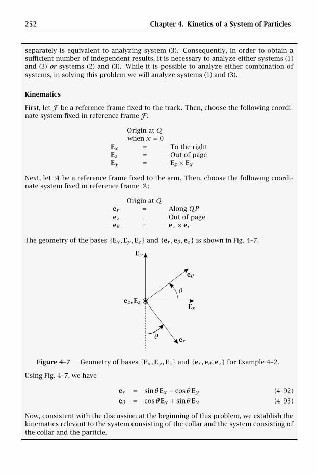
252 Chapter 4. Kinetics of a System of Particles
separately is equivalent to analyzing system (3). Consequently, in order to obtain asufficient number of independent results, it is necessary to analyze either systems (1)and (3) or systems (2) and (3). While it is possible to analyze either combination ofsystems, in solving this problem we will analyze systems (1) and (3).
Kinematics
First, let F be a reference frame fixed to the track. Then, choose the following coordi-nate system fixed in reference frame F :
Origin at Qwhen x = 0
Ex = To the rightEz = Out of pageEy = Ez × Ex
Next, let A be a reference frame fixed to the arm. Then, choose the following coordi-nate system fixed in reference frame A:
Origin at Qer = Along QPez = Out of pageeθ = ez × er
The geometry of the bases Ex,Ey,Ez and er ,eθ,ez is shown in Fig. 4–7.
er
eθ
Ex
Ey
ez,Ez
θ
θ
Figure 4–7 Geometry of bases Ex,Ey,Ez and er ,eθ,ez for Example 4–2.
Using Fig. 4–7, we have
er = sinθEx − cosθEy (4–92)
eθ = cosθEx + sinθEy (4–93)
Now, consistent with the discussion at the beginning of this problem, we establish thekinematics relevant to the system consisting of the collar and the system consisting ofthe collar and the particle.

4.5 Rate of Change of Angular Momentum for a System of Particles 253
Kinematics of Collar
The position of the collar is given as
r1 = xEx (4–94)
Computing the rate of change of r1 in reference frame F , we obtain the velocity of thecollar in reference frame F as
Fv1 =Fddt(r1) = xEx (4–95)
Finally, computing the rate of change of Fv1 in reference frame F , we obtain theacceleration of the collar in reference frame F as
Fa1 =Fddt
(Fv1
)= xEx (4–96)
Kinematics of Particle
The kinematics of the collar-particle system are governed by the motion of the centerof mass of the system. Consequently, in order to determine the kinematics of the cen-ter of mass of the collar-particle system, it is first necessary to determine the position,velocity, and The position of the particle is given as
r2 = r1 + r2/1 (4–97)
Now we haver2/1 = ler (4–98)
Then, adding Eqs. (4–98) and (4–97), we obtain the position of the particle as
r2 = xEx + ler (4–99)
Next, the angular velocity of reference frame A in reference frame F is given as
FωA = θez (4–100)
Consequently, the velocity of the particle in reference frame F is obtained as
Fv2 =Fddt(r2) =
Fddt(r1)+
Fddt
(r2/1
) = Fv1 + Fv2/1 (4–101)
We already have Fv1 from Eq. (4–95). Applying the rate of change transport theoremto r2/1 between reference frames A and F gives
Fv2/1 =Fddt
(r2/1
) = A ddt
(r2/1
)+ FωA × r2/1 (4–102)
Now we have
A ddt
(r2/1
) = 0 (4–103)
FωA × r2/1 = θez × ler = lθeθ (4–104)
254 Chapter 4. Kinetics of a System of Particles
Adding Eqs. (4–103) and (4–104), we obtain the velocity of the particle relative to thecollar in reference frame F as
Fv2/1 = lθeθ (4–105)
Then, substituting the results of Eqs. (4–95) and (4–105) into Eq. (4–101), we obtain thevelocity of the particle in reference frame F as
Fv2 = xEx + lθeθ (4–106)
Computing the rate of change of Fv2 in reference frameF using the general expressionfor Fv2 as given in Eq. (4–101), the acceleration of the particle in reference frame F isgiven as
Fa2 =Fddt
(Fv2
)=Fddt
(Fv1
)+Fddt
(Fv2/1
)= Fa1 + Fa2/1 (4–107)
Now we already have Fa1 from Eq. (4–96). Applying the rate of change transport theo-rem between reference frames A and F , we obtain Fa2/1 as
Fa2/1 =Fddt
(Fv2/1
)=A ddt
(Fv2/1
)+ FωA × Fv2/1 (4–108)
Now we have
A ddt
(Fv2/1
)= lθeθ (4–109)
FωA × Fv2/1 = θez × lθeθ = −lθ2er (4–110)
Adding Eqs. (4–109) and (4–110), we obtain
Fa2/1 = −lθ2er + lθeθ (4–111)
Finally, adding Eqs. (4–111) and (4–96), we obtain the acceleration of the particle inreference frame F as
Fa2 = xEx − lθ2er + lθeθ (4–112)
Kinematics of Center of Mass of Collar-Particle System
The position of the center of mass of the collar-particle system is given as
r = m1r1 +m2r2
m1 +m2(4–113)
Substituting the expressions for r1 and r2 from Eqs. (4–94) and (4–97), respectively,into (4–113), we obtain r as
r = m1xEx +m2(xEx + ler )m1 +m2
= xEx + m2
m1 +m2ler (4–114)
Next, the velocity of the center of mass of the collar-particle system in reference frameF is given as
Fv = m1Fv1 +m2
Fv2
m1 +m2(4–115)
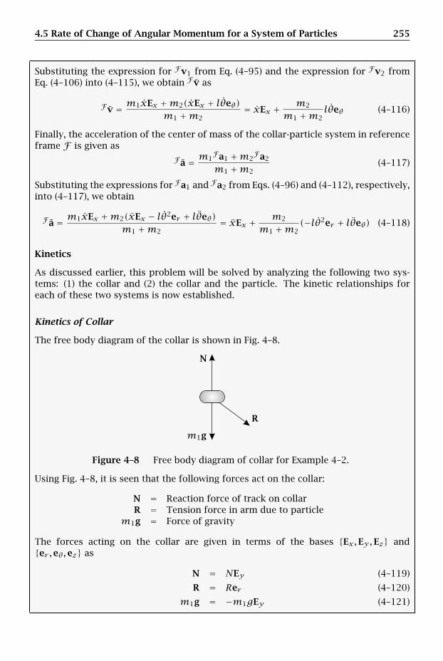
4.5 Rate of Change of Angular Momentum for a System of Particles 255
Substituting the expression for Fv1 from Eq. (4–95) and the expression for Fv2 fromEq. (4–106) into (4–115), we obtain Fv as
Fv = m1xEx +m2(xEx + lθeθ)m1 +m2
= xEx + m2
m1 +m2lθeθ (4–116)
Finally, the acceleration of the center of mass of the collar-particle system in referenceframe F is given as
Fa = m1Fa1 +m2
Fa2
m1 +m2(4–117)
Substituting the expressions for Fa1 and Fa2 from Eqs. (4–96) and (4–112), respectively,into (4–117), we obtain
Fa = m1xEx +m2(xEx − lθ2er + lθeθ)m1 +m2
= xEx + m2
m1 +m2(−lθ2er + lθeθ) (4–118)
Kinetics
As discussed earlier, this problem will be solved by analyzing the following two sys-tems: (1) the collar and (2) the collar and the particle. The kinetic relationships foreach of these two systems is now established.
Kinetics of Collar
The free body diagram of the collar is shown in Fig. 4–8.
N
R
m1g
Figure 4–8 Free body diagram of collar for Example 4–2.
Using Fig. 4–8, it is seen that the following forces act on the collar:
N = Reaction force of track on collarR = Tension force in arm due to particle
m1g = Force of gravity
The forces acting on the collar are given in terms of the bases Ex,Ey,Ez ander ,eθ,ez as
N = NEy (4–119)
R = Rer (4–120)
m1g = −m1gEy (4–121)
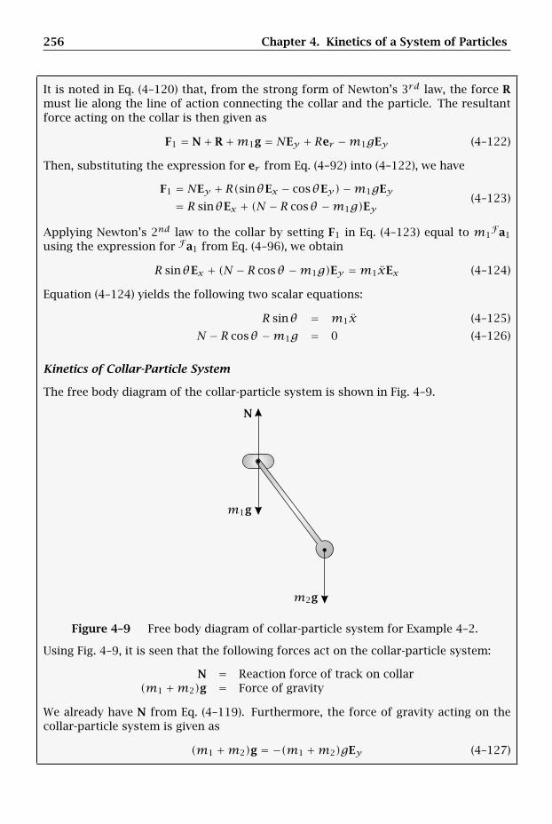
256 Chapter 4. Kinetics of a System of Particles
It is noted in Eq. (4–120) that, from the strong form of Newton’s 3rd law, the force Rmust lie along the line of action connecting the collar and the particle. The resultantforce acting on the collar is then given as
F1 = N+ R+m1g = NEy + Rer −m1gEy (4–122)
Then, substituting the expression for er from Eq. (4–92) into (4–122), we have
F1 = NEy + R(sinθEx − cosθEy)−m1gEy= R sinθEx + (N − R cosθ −m1g)Ey
(4–123)
Applying Newton’s 2nd law to the collar by setting F1 in Eq. (4–123) equal to m1Fa1
using the expression for Fa1 from Eq. (4–96), we obtain
R sinθEx + (N − R cosθ −m1g)Ey =m1xEx (4–124)
Equation (4–124) yields the following two scalar equations:
R sinθ = m1x (4–125)
N − R cosθ −m1g = 0 (4–126)
Kinetics of Collar-Particle System
The free body diagram of the collar-particle system is shown in Fig. 4–9.
N
m1g
m2g
Figure 4–9 Free body diagram of collar-particle system for Example 4–2.
Using Fig. 4–9, it is seen that the following forces act on the collar-particle system:
N = Reaction force of track on collar(m1 +m2)g = Force of gravity
We already have N from Eq. (4–119). Furthermore, the force of gravity acting on thecollar-particle system is given as
(m1 +m2)g = −(m1 +m2)gEy (4–127)
4.5 Rate of Change of Angular Momentum for a System of Particles 257
Consequently, the resultant force acting on the collar is given as
F = N+ (m1 +m2)g = NEy − (m1 +m2)gEy =[N − (m1 +m2)g
]Ey (4–128)
Applying Newton’s 2nd law to the collar-particle system by setting F in Eq. (4–128)equal to (m1 +m2)Fa using the expression for Fa from Eq. (4–118), we obtain
[N − (m1 +m2)g
]Ey = (m1 +m2)
[xEx + m2
m1 +m2(−lθ2er + lθeθ)
](4–129)
Equation (4–129) can be rewritten as[N − (m1 +m2)g
]Ey = (m1 +m2)xEx −m2lθ2er +m2lθeθ (4–130)
Then, substituting the expressions for er and eθ from Eqs. (4–92) and (4–93), respec-tively, into Eq. (4–130), we obtain
[N − (m1 +m2)g
]Ey = (m1 +m2)xEx −m2lθ2(sinθEx − cosθEy)
+m2lθ(cosθEx + sinθEy)(4–131)
Rearranging Eq. (4–131), we obtain
[N − (m1 +m2)g
]Ey =
[(m1 +m2)x +m2lθ cosθ −m2lθ2 sinθ
]Ex
+[m2lθ sinθ +m2lθ2 cosθ
]Ey
(4–132)
Equation (4–132) yields the following two scalar equations:
0 = (m1 +m2)x +m2lθ cosθ −m2lθ2 sinθ (4–133)
N − (m1 +m2)g = m2lθ sinθ +m2lθ2 cosθ (4–134)
(a) System of Two Differential Equations
Using the results of Eqs. (4–125), (4–126), (4–133), and (4–134), a system of two differ-ential equations is now determined. Because Eq. (4–133) has no unknown forces, it isthe first differential equation. The second differential equation is obtained as follows.Multiplying Eqs. (4–125) and (4–126) by cosθ and sinθ , respectively, we have
R sinθ cosθ = m1x cosθ (4–135)
N sinθ − R cosθ sinθ −m1g sinθ = 0 (4–136)
Adding Eqs. (4–135) and (4–136), we obtain
N sinθ −m1g sinθ =m1x cosθ (4–137)
Next, multiplying Eq. (4–134) by sinθ gives
N sinθ − (m1 +m2)g sinθ =m2lθ sin2θ +m2lθ2 cosθ sinθ (4–138)
Then, subtracting Eq. (4–138) from (4–137), we obtain
m2g sinθ =m1x cosθ −m2lθ sin2θ −m2lθ2 cosθ sinθ (4–139)
258 Chapter 4. Kinetics of a System of Particles
Rearranging Eq. (4–139), we obtain the second differential equation of motion as
m1x cosθ −m2lθ sin2θ −m2lθ2 cosθ sinθ −m2g sinθ = 0 (4–140)
A system of two differential equations that describes the motion of the collar-particlesystem is then given as
(m1 +m2)x +m2lθ cosθ −m2lθ2 sinθ = 0 (4–141)
m1x cosθ −m2lθ sin2θ −m2lθ2 cosθ sinθ −m2g sinθ = 0 (4–142)
(b) Alternate System of Differential Equations
While Eqs. (4–141) and (4–142) are independent, a slightly simpler set of equations canbe derived by manipulating Eqs. (4–141) and (4–142) as follows. Multiplying Eq. (4–141)by cosθ , we have
(m1 +m2)x cosθ +m2lθ cos2θ −m2lθ2 sinθ cosθ = 0 (4–143)
m1x cosθ −m2lθ sin2θ −m2lθ2 cosθ sinθ −m2g sinθ = 0 (4–144)
Then, subtracting Eq. (4–144) from (4–143), we obtain
m2x cosθ +m2lθ(cos2θ + sin2θ)+m2g sinθ = 0 (4–145)
Simplifying Eq. (4–145), we obtain
m2x cosθ +m2lθ +m2g sinθ = 0 (4–146)
Now, because the two differential equations in Eqs. (4–141) and (4–142) are indepen-dent and we have obtained Eqs. (4–141) and (4–146) via a nonsingular transformation,the two differential equations in Eqs. (4–141) and (4–146) are also independent. Con-sequently, an alternate system of two differential equations describing the motion ofthe collar-particle system is given as
(m1 +m2)x +m2lθ cosθ −m2lθ2 sinθ = 0 (4–147)
m2x cosθ +m2lθ +m2g sinθ = 0 (4–148)
(c) Determination of One Differential Equation via Balance of Angular MomentumRelative to Collar
It was seen above that the two differential equations of motion were obtained purelyby using Newton’s 2nd law. However, it is useful to note that the one of the differentialequations can also be obtained by performing a balance of angular momentum of thecollar-particle system relative to the collar. Observing that the collar is not an inertiallyfixed point, it is necessary to apply Eq. (4–87) as
M1 − (r− r1)× (m1 +m2)Fa1 =Fddt
(FH1
)(4–149)
where M1 is the resultant moment applied to the collar-particle system relative to the
collar whileFd(FH1)/dt is the rate of change of angular momentum of the collar-
particle system relative to the collar. First, the rate of change of angular momentum

4.5 Rate of Change of Angular Momentum for a System of Particles 259
of the collar-particle system relative to the collar is given from Eq. (4–79) as
Fddt
(FH1
)= (r1 − r1)×m1(Fa1 − Fa1)+ (r2 − r1)×m2(Fa2 − Fa1) (4–150)
Observing that the first term in Eq. (4–150) is zero, we have
Fddt
(FH1
)= (r2 − r1)×m2(Fa2 − Fa1) (4–151)
Using the expressions for r1 and r2 from Eqs. (4–94) and (4–97), respectively, we have
r2 − r1 = ler (4–152)
Next, using the expressions for Fa2 and Fa1 from Eqs. (4–96) and (4–112), respectively,we have
Fa2 − Fa1 = −lθ2er + lθeθ (4–153)
Consequently, we obtain
Fddt
(FH1
)= ler ×m2(−lθ2er + lθeθ) =m2l2θez (4–154)
Next, observing from the free body diagram of the collar-particle system in Fig. 4–9that the forces N and m1g pass through the collar, the resultant moment relative tothe collar is due entirely to m2g and is given as
M1 = (r2 − r1)×m2g = ler × (−m2gEy)= −m2gl(sinθEx − cosθEy)× Ey = −m2gl sinθez
(4–155)
Finally, using the expressions for r and Fa1 from Eqs. (4–114) and (4–96), respectively,the inertial moment due to the acceleration of the collar is given as
−(r− r1)× (m1 +m2)Fa1 = − m2
m1 +m2ler × (m1 +m2)× (xEx)
= −m2lxer × Ex = −m2lx(sinθEx − cosθEy)× Ex= −m2lx cosθez
(4–156)
where we have used the expression for er from Eq. (4–92) in (4–156). Substituting theresults of Eqs. (4–154), (4–155), and (4–156) into Eq. (4–149), we obtain
m2l2θez = −m2gl sinθez −m2lx cosθez (4–157)
Rearranging and dropping the dependence on ez in Eq. (4–157), we obtain
m2lx cosθ +m2l2θ +m2gl sinθ = 0 (4–158)
Finally, dropping the common factor of l from Eq. (4–158), the second differentialequation is obtained as
m2x cosθ +m2lθ +m2g sinθ = 0 (4–159)
It is seen that Eq. (4–159) is identical to Eq. (4–148).
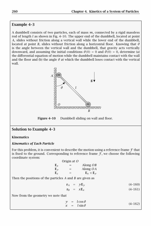
260 Chapter 4. Kinetics of a System of Particles
Example 4–3
A dumbbell consists of two particles, each of mass m, connected by a rigid masslessrod of length l as shown in Fig. 4–10. The upper end of the dumbbell, located at pointA, slides without friction along a vertical wall while the lower end of the dumbbell,located at point B, slides without friction along a horizontal floor. Knowing that θis the angle between the vertical wall and the dumbbell, that gravity acts verticallydownward, and assuming the initial conditions θ(0) = 0 and θ(0) = 0, determine (a)the differential equation of motion while the dumbbell maintains contact with the walland the floor and (b) the angle θ at which the dumbbell loses contact with the verticalwall.
g
l
m
mA
B
O
θ
Figure 4–10 Dumbbell sliding on wall and floor.
Solution to Example 4–3
Kinematics
Kinematics of Each Particle
For this problem, it is convenient to describe the motion using a reference frameF thatis fixed to the ground. Corresponding to reference frame F , we choose the followingcoordinate system:
Origin at OEx = Along OBEy = Along OAEz = Ex × Ey
Then the positions of the particles A and B are given as
rA = yEy (4–160)
rB = xEx (4–161)
Now from the geometry we note that
y = l cosθx = l sinθ (4–162)
4.5 Rate of Change of Angular Momentum for a System of Particles 261
Therefore, the positions are given as
rA = l cosθEy (4–163)
rB = l sinθEx (4–164)
Noting that reference frame F is fixed, the velocities of the particles in reference frameF are obtained as
FvA =Fddt(rA) = −lθ sinθEy (4–165)
FvB =Fddt(rB) = lθ cosθEx (4–166)
Computing the rate of change of FvA and FvB in Eqs. (4–165) and (4–166), respectively,we obtain the accelerations of the particles in reference frame F as
FaA =Fddt
(FvA
)= −l(θ sinθ + θ2 cosθ)Ey (4–167)
FaB =Fddt
(FvB
)= l(θ cosθ − θ2 sinθ)Ex (4–168)
Kinematics of Center of Mass of Dumbbell
The position of the center of mass of the rod is given as
r = mArA +mBrBmA +mB
(4–169)
Substituting the expression for rA and rB from Eqs. (4–163) and (4–164), respectively,and noting that mA =mB =m, we obtain r as
r = ml cosθEy +ml sinθEx2m
= l2
sinθEx + l2 cosθEy (4–170)
Furthermore, the velocity of the center of mass is given as
Fv = mAFvA +mB
FvAmA +mB
= l2θ cosθEx − l2 θ sinθEy (4–171)
Then the acceleration of the center of mass is given as
Fa = mAFaA +mB
FaAmA +mB
= l2(θ cosθ − θ2 sinθ)Ex − l2(θ sinθ + θ2 cosθ)Ey (4–172)
Kinematics Relative to Center of Mass of Dumbbell
In order to solve this problem we will also need to perform a balance of angular mo-mentum. Given the geometry of this problem, it is convenient to choose the center ofmass of the system as the reference point. Correspondingly, the angular momentumof the system relative to the center of mass of the rod in reference frame F is given as
FH = (rA − r)×mA(FvA − Fv)+ (rB − r)×mB(FvB − Fv) (4–173)
262 Chapter 4. Kinetics of a System of Particles
Using the expressions for rA and rB from Eqs. (4–163) and (4–164), respectively, andthe expression for r from Eq. (4–170), we have
rA − r = − l2
sinθEx + l2 cosθEy
rB − r = l2
sinθEx − l2 cosθEy(4–174)
Furthermore, using the expressions for FvA, FvB , and Fv from Eqs. (4–165), (4–166),and (4–171), respectively, we obtain
FvA − Fv = − l2θ cosθEx − l2 θ sinθEy
FvB − Fv = l2θ cosθEx + l2 θ sinθEy
(4–175)
Finally, substituting the results of Eqs. (4–174) and (4–175) into (4–173) and using thefact that mA =mB =m, we obtain
FH as
FH =
(− l
2sinθEx + l2 cosθEy
)×m
(− l
2θ cosθEx − l2 θ sinθEy
)
+(l2
sinθEx − l2 cosθEy
)×m
(l2θ cosθEx + l2 θ sinθEy
) (4–176)
Simplifying Eq. (4–176) gives
FH = ml
2
2θEz (4–177)
Computing the rate of change ofF
H in reference frame F , we obtain
Fddt
(FH)≡ F ˙H = ml
2
2θEz (4–178)
Kinetics
It is convenient to solve this problem by applying the following two balance laws for asystem of particles: (1) Newton’s 2nd law to the center of mass of the dumbbell and (2)a balance of angular momentum relative to the center of mass of the dumbbell. Eachof these balance laws is now applied.
Application of Newton’s 2nd Law to Center of Mass of Dumbbell
The free body diagram of the system is shown in Fig. 4–11.
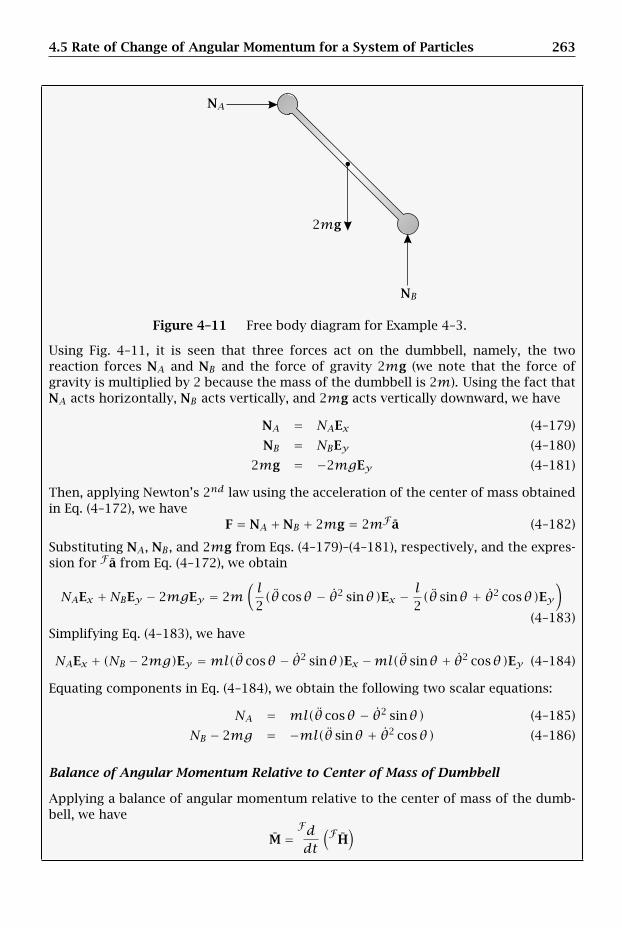
4.5 Rate of Change of Angular Momentum for a System of Particles 263
NA
NB
2mg
Figure 4–11 Free body diagram for Example 4–3.
Using Fig. 4–11, it is seen that three forces act on the dumbbell, namely, the tworeaction forces NA and NB and the force of gravity 2mg (we note that the force ofgravity is multiplied by 2 because the mass of the dumbbell is 2m). Using the fact thatNA acts horizontally, NB acts vertically, and 2mg acts vertically downward, we have
NA = NAEx (4–179)
NB = NBEy (4–180)
2mg = −2mgEy (4–181)
Then, applying Newton’s 2nd law using the acceleration of the center of mass obtainedin Eq. (4–172), we have
F = NA +NB + 2mg = 2mFa (4–182)
Substituting NA, NB , and 2mg from Eqs. (4–179)–(4–181), respectively, and the expres-sion for Fa from Eq. (4–172), we obtain
NAEx +NBEy − 2mgEy = 2m(l2(θ cosθ − θ2 sinθ)Ex − l2(θ sinθ + θ2 cosθ)Ey
)(4–183)
Simplifying Eq. (4–183), we have
NAEx + (NB − 2mg)Ey =ml(θ cosθ − θ2 sinθ)Ex −ml(θ sinθ + θ2 cosθ)Ey (4–184)
Equating components in Eq. (4–184), we obtain the following two scalar equations:
NA = ml(θ cosθ − θ2 sinθ) (4–185)
NB − 2mg = −ml(θ sinθ + θ2 cosθ) (4–186)
Balance of Angular Momentum Relative to Center of Mass of Dumbbell
Applying a balance of angular momentum relative to the center of mass of the dumb-bell, we have
M =Fddt
(FH)
264 Chapter 4. Kinetics of a System of Particles
where M is the moment due to all external forces relative to the center of mass. Notingthat gravity acts at the center of mass, M is due entirely to the reaction forces NA andNB . Consequently, we have
M = (rA − r)×NA + (rB − r)×NB (4–187)
Using rA − r and rB − r from Eq. (4–170), we obtain
M =(− l
2sinθEx + l2 cosθEy
)×NAEx +
(l2
sinθEx − l2 cosθEy
)×NBEy (4–188)
Simplifying Eq. (4–188), we obtain
M =(− l
2cosθNA + l2 sinθNB
)Ez (4–189)
Setting M from Eq. (4–188) equal toF ˙H from Eq. (4–178) gives
(− l
2cosθNA + l2 sinθNB
)Ez = ml
2
2θEz (4–190)
Dropping the dependence on Ez in Eq. (4–190), we obtain the scalar equation
− l2
cosθNA + l2 sinθNB = ml2
2θ (4–191)
Dropping the common factor of l/2, Eq. (4–191) simplifies to
−NA cosθ +NB sinθ =mlθ (4–192)
(a) Differential Equation While Dumbbell Maintains Contact with Vertical Wall
Equations (4–185), (4–186), and (4–192) can now be used together to obtain the dif-ferential equation of motion. Multiplying Eqs. (4–185) and (4–186) by cosθ and sinθ ,respectively, and subtracting the result, we obtain
NA cosθ −NB sinθ + 2mg sinθ =ml(θ cosθ − θ2 sinθ) cosθ
+ml(θ sinθ + θ2 cosθ) sinθ(4–193)
Equation (4–193) simplifies to
NA cosθ −NB sinθ = −2mg sinθ +mlθ (4–194)
Then, adding Eqs. (4–194) and (4–192), we obtain
2mlθ − 2mg sinθ = 0 (4–195)
Simplifying Eq. (4–195), we obtain the differential equation of motion as
θ − gl
sinθ = 0 (4–196)
4.5 Rate of Change of Angular Momentum for a System of Particles 265
(b) Angle θ at Which Dumbbell Loses Contact with Vertical Wall
We note that the rod will lose contact with the vertical wall when NA = 0, which, fromEq. (4–185), implies that
θ cosθ − θ2 sinθ = 0 (4–197)
Now, because we want to solve for the angle θ at which contact is lost, in order tomake Eq. (4–197) an algebraic equation, we need to obtain expressions for θ2 and θ asfunctions of θ. We can get θ as a function of θ simply by rearranging Eq. (4–196) as
θ = gl
sinθ (4–198)
We note that θ = θdθ/dθ. Therefore, Eq. (4–198) can be rewritten as
θdθdθ
= gl
sinθ (4–199)
Separating variables in Eq. (4–199) gives
θdθ = gl
sinθdθ (4–200)
Integrating both sides of Eq. (4–200) gives
∫ θθ0
ηdη =∫ θθ0
gl
sinνdν (4–201)
where η and ν are dummy variables of integration. From Eq. (4–201) we have
η2
2
∣∣∣∣∣θ
θ0
= −gl
cosν∣∣∣∣θθ0
(4–202)
Equation (4–202) gives
θ2 − θ20 = −
2gl(cosθ − cosθ0) (4–203)
Rearranging Eq. (4–203), we obtain
θ2 = θ20 +
2gl(cosθ 0 − cosθ) (4–204)
Substituting θ2 and θ from Eq. (4–204) and Eq. (4–198), respectively, into Eq. (4–197)gives
gl
sinθ cosθ −(θ2
0 +2gl(cosθ 0 − cosθ)
)sinθ = 0 (4–205)
Then, using the given initial conditions θ(t = 0) = 0 and θ(t = 0) = 0, Eq. (4–205)simplifies to
gl
sinθ cosθ − 2gl(1− cosθ) sinθ = 0 (4–206)
Dropping g and l from Eq. (4–206) and simplifying, we obtain
sinθ cosθ − 2(1− cosθ) sinθ = 0 (4–207)

266 Chapter 4. Kinetics of a System of Particles
Equation (4–207) can be written as
sinθ (3 cosθ − 2) = 0 (4–208)
which implies that either sinθ = 0 or 3 cosθ − 2 = 0. However, we note that the casesinθ = 0 implies that θ = 0, which corresponds to the instant when the dumbbell isvertical and, therefore, has not yet begun its motion. Therefore, the dumbbell will losecontact with the vertical wall when
3 cosθ − 2 = 0 (4–209)
Solving Eq. (4–209) for θ, we obtain
θ = cos−1(2/3) ≈ 48.1897 deg (4–210)
We note that any similarity between Eqs. (4–210) and (3–173) on page 176 from Exam-ple 3–4 is purely coincidental.
4.6 Impulse and Momentum for a System of Particles
4.6.1 Linear Impulse and Linear Momentum for a System of Particles
Consider again Eq. (4–38) from Section 4.3, i.e.,
F =mNa (4–211)
Suppose now that we consider motion over a time interval t ∈ [t1, t2]. Then, integrat-ing Eq. (4–211) from t1 to t2 gives
∫ t2t1
Fdt =∫ t2t1mNadt =m(Nv(t2)−Nv(t1)) =mNv2 −mNv1 (4–212)
Now from Eq. (4–9) we have
NG =mNv =n∑i=1
miNvi =
n∑i=1
NGi (4–213)
whereNGi =mi
Nvi (i = 1, . . . , n) (4–214)
are the linear momenta of each particle in the system. In other words, the linearmomentum of a system of particles is the sum of the linear momenta of each particlein the system. Furthermore, as we saw in Chapter 3, the quantity
∫ t2t1
Fdt
4.6 Impulse and Momentum for a System of Particles 267
is the linear impulse of the total external force F applied to the system on the timeinterval t ∈ [t1, t2]. Defining
F ≡∫ t2t1
Fdt (4–215)
we have
F = NG(t2)−NG(t1) (4–216)
Equation (4–216) is called the principle of linear impulse and linear momentum for asystem of particles.
4.6.2 Angular Impulse and Angular Momentum for a System of Particles
Consider again the result of Eq. (4–87) from Section 4.5, i.e.,
MQ − (r− rQ)×mNaQ =Nddt
(NHQ
)(4–217)
Suppose now that we consider motion over a time interval t ∈ [t1, t2]. Then, integrat-ing Eq. (4–217), we obtain
∫ t2t1
[MQ − (r− rQ)×mNaQ
]dt =
∫ t2t1
Nddt
(NHQ
)dt (4–218)
We observe that the first term in Eq. (4–218) is the angular impulse applied to thesystem relative to point Q, i.e.,
MQ =∫ t2t1
MQdt (4–219)
Furthermore, the right-hand side of Eq. (4–218) is the difference between the angularmomentum relative to Q at t2 and t1, i.e.,
NHQ(t2)−NHQ(t1) =∫ t2t1
Nddt
(NHQ
)dt (4–220)
Equation (4–218) then becomes
MQ −∫ t2t1(r− rQ)×mNaQdt = NHQ(t2)−NHQ(t1) (4–221)
which is the principle of angular impulse and angular momentum for a system of par-ticles relative to an arbitrary reference point Q. It is noted that the quantity
−∫ t2t1(r− rQ)×mNaQdt (4–222)
is called the inertial angular impulse of the reference point Q relative to the center ofmass on the time interval t ∈ [t1, t2].
Now suppose that we choose a point O fixed in an inertial reference frame N asthe reference point. Because the acceleration of point O inN is zero, i.e., NaO = 0, the
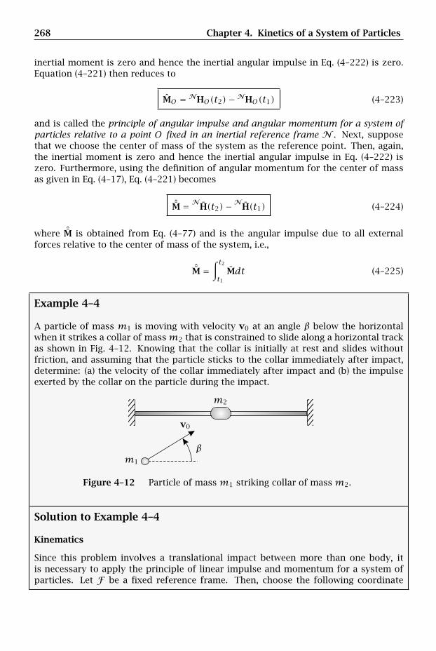
268 Chapter 4. Kinetics of a System of Particles
inertial moment is zero and hence the inertial angular impulse in Eq. (4–222) is zero.Equation (4–221) then reduces to
MO = NHO(t2)−NHO(t1) (4–223)
and is called the principle of angular impulse and angular momentum for a system ofparticles relative to a point O fixed in an inertial reference frame N . Next, supposethat we choose the center of mass of the system as the reference point. Then, again,the inertial moment is zero and hence the inertial angular impulse in Eq. (4–222) iszero. Furthermore, using the definition of angular momentum for the center of massas given in Eq. (4–17), Eq. (4–221) becomes
ˆM = NH(t2)−N
H(t1) (4–224)
where ˆM is obtained from Eq. (4–77) and is the angular impulse due to all externalforces relative to the center of mass of the system, i.e.,
ˆM =∫ t2t1
Mdt (4–225)
Example 4–4
A particle of mass m1 is moving with velocity v0 at an angle β below the horizontalwhen it strikes a collar of massm2 that is constrained to slide along a horizontal trackas shown in Fig. 4–12. Knowing that the collar is initially at rest and slides withoutfriction, and assuming that the particle sticks to the collar immediately after impact,determine: (a) the velocity of the collar immediately after impact and (b) the impulseexerted by the collar on the particle during the impact.
v0
m1
m2
β
Figure 4–12 Particle of mass m1 striking collar of mass m2.
Solution to Example 4–4
Kinematics
Since this problem involves a translational impact between more than one body, itis necessary to apply the principle of linear impulse and momentum for a system ofparticles. Let F be a fixed reference frame. Then, choose the following coordinate
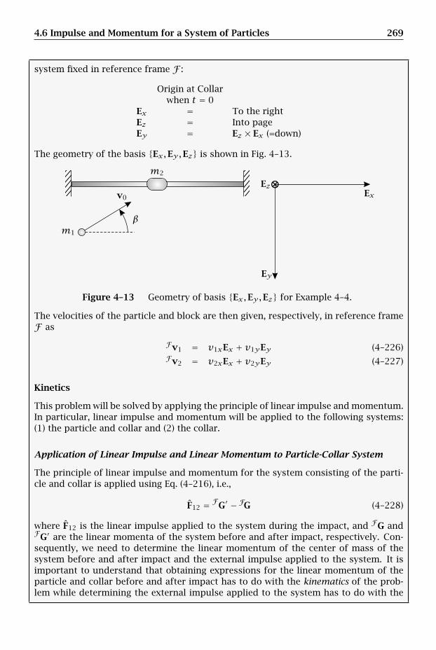
4.6 Impulse and Momentum for a System of Particles 269
system fixed in reference frame F :
Origin at Collarwhen t = 0
Ex = To the rightEz = Into pageEy = Ez × Ex (=down)
The geometry of the basis Ex,Ey,Ez is shown in Fig. 4–13.
⊗Ex
Ey
Ezv0
m1
m2
β
Figure 4–13 Geometry of basis Ex,Ey,Ez for Example 4–4.
The velocities of the particle and block are then given, respectively, in reference frameF as
Fv1 = v1xEx + v1yEy (4–226)Fv2 = v2xEx + v2yEy (4–227)
Kinetics
This problem will be solved by applying the principle of linear impulse and momentum.In particular, linear impulse and momentum will be applied to the following systems:(1) the particle and collar and (2) the collar.
Application of Linear Impulse and Linear Momentum to Particle-Collar System
The principle of linear impulse and momentum for the system consisting of the parti-cle and collar is applied using Eq. (4–216), i.e.,
F12 = FG′ − FG (4–228)
where F12 is the linear impulse applied to the system during the impact, and FG andFG′ are the linear momenta of the system before and after impact, respectively. Con-sequently, we need to determine the linear momentum of the center of mass of thesystem before and after impact and the external impulse applied to the system. It isimportant to understand that obtaining expressions for the linear momentum of theparticle and collar before and after impact has to do with the kinematics of the prob-lem while determining the external impulse applied to the system has to do with the

270 Chapter 4. Kinetics of a System of Particles
kinetics of the problem. The linear momentum of the center of mass before impact isfound as
FG = (m1 +m2)Fv =m1Fv1 +m2
Fv2 (4–229)
Using the chosen coordinate system Ex,Ey,Ez, the velocity of the particle beforeimpact is given in terms of the angle β as
Fv1 = v0 = v0 cosβEx − v0 sinβEy (4–230)
where v0 = ‖v0‖. Next, because the collar is initially motionless, its velocity beforeimpact is given as
Fv2 = 0 (4–231)
Since the velocities of the particle and the collar after impact are unknown, we canwrite
Fv′1 = v′1xEx + v′1yEyFv′2 = v′2xEx + v′2yEy
(4–232)
Furthermore, because the particle sticks to the collar on impact, the post-impact ve-locity of the particle and collar must be the same. Consequently,
Fv′1 = Fv′2 = v′ = v′xEx + v′yEy (4–233)
Also, because the system must move in the Ex-direction after impact, we have
v′y = 0 (4–234)
Consequently, the post-impact velocity of the particle and collar can be written as
Fv′ = v′xEx (4–235)
where v′x has yet to be determined.The external impulse applied to the particle-collar system is determined by exam-
ining the free body diagram of the system during impact as shown in Fig. 4–14.
R
Figure 4–14 Free body diagram of system consisting of particle and collar duringimpact for Example 4–4.
It can be seen that the only impulse that is external to the particle-collar system isthe reaction impulse, R, of the track. Because the collar slides without friction, thisreaction impulse of the track on the particle-collar system can be written as
R = REy (4–236)
Consequently, the total external impulse applied to the system, denoted F12, is givenas
F12 = R = REy (4–237)
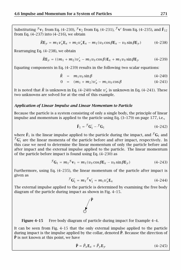
4.6 Impulse and Momentum for a System of Particles 271
Substituting Fv1 from Eq. (4–230), Fv2 from Eq. (4–231), Fv′ from Eq. (4–235), and F12
from Eq. (4–237) into (4–216), we obtain
REy =m1v′xEx +m2v′xEx −m1(v0 cosβEx − v0 sinβEy) (4–238)
Rearranging Eq. (4–238), we obtain
REy = ((m1 +m2)v′x −m1v0 cosβ)Ex +m1v0 sinβEy (4–239)
Equating components in Eq. (4–239) results in the following two scalar equations:
R = m1v0 sinβ (4–240)
0 = (m1 +m2)v′x −m1v0 cosβ (4–241)
It is noted that R is unknown in Eq. (4–240) while v′x is unknown in Eq. (4–241). Thesetwo unknowns are solved for at the end of this example.
Application of Linear Impulse and Linear Momentum to Particle
Because the particle is a system consisting of only a single body, the principle of linearimpulse and momentum is applied to the particle using Eq. (3–179) on page 177, i.e.,
F1 = FG′1 − FG1 (4–242)
where F1 is the linear impulse applied to the particle during the impact, and FG1 andFG′1 are the linear momenta of the particle before and after impact, respectively. Inthis case we need to determine the linear momentum of only the particle before andafter impact and the external impulse applied to the particle. The linear momentumof the particle before impact is found using Eq. (4–230) as
FG1 =m1Fv1 =m1(v0 cosβEx − v0 sinβEy) (4–243)
Furthermore, using Eq. (4–235), the linear momentum of the particle after impact isgiven as
FG′1 =m1Fv′1 =m1v′xEx (4–244)
The external impulse applied to the particle is determined by examining the free bodydiagram of the particle during impact as shown in Fig. 4–15.
P
Figure 4–15 Free body diagram of particle during impact for Example 4–4.
It can be seen from Fig. 4–15 that the only external impulse applied to the particleduring impact is the impulse applied by the collar, denoted P. Because the direction ofP is not known at this point, we have
P = PxEx + PyEy (4–245)
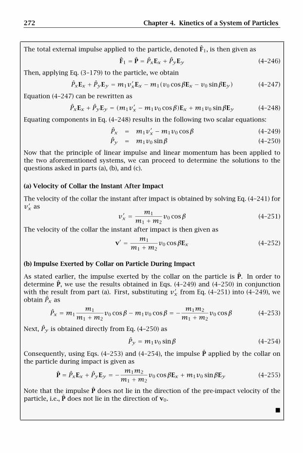
272 Chapter 4. Kinetics of a System of Particles
The total external impulse applied to the particle, denoted F1, is then given as
F1 = P = PxEx + PyEy (4–246)
Then, applying Eq. (3–179) to the particle, we obtain
PxEx + PyEy =m1v′xEx −m1(v0 cosβEx − v0 sinβEy) (4–247)
Equation (4–247) can be rewritten as
PxEx + PyEy = (m1v′x −m1v0 cosβ)Ex +m1v0 sinβEy (4–248)
Equating components in Eq. (4–248) results in the following two scalar equations:
Px = m1v′x −m1v0 cosβ (4–249)
Py = m1v0 sinβ (4–250)
Now that the principle of linear impulse and linear momentum has been applied tothe two aforementioned systems, we can proceed to determine the solutions to thequestions asked in parts (a), (b), and (c).
(a) Velocity of Collar the Instant After Impact
The velocity of the collar the instant after impact is obtained by solving Eq. (4–241) forv′x as
v′x =m1
m1 +m2v0 cosβ (4–251)
The velocity of the collar the instant after impact is then given as
v′ = m1
m1 +m2v0 cosβEx (4–252)
(b) Impulse Exerted by Collar on Particle During Impact
As stated earlier, the impulse exerted by the collar on the particle is P. In order todetermine P, we use the results obtained in Eqs. (4–249) and (4–250) in conjunctionwith the result from part (a). First, substituting v′x from Eq. (4–251) into (4–249), weobtain Px as
Px =m1m1
m1 +m2v0 cosβ−m1v0 cosβ = − m1m2
m1 +m2v0 cosβ (4–253)
Next, Py is obtained directly from Eq. (4–250) as
Py =m1v0 sinβ (4–254)
Consequently, using Eqs. (4–253) and (4–254), the impulse P applied by the collar onthe particle during impact is given as
P = PxEx + PyEy = − m1m2
m1 +m2v0 cosβEx +m1v0 sinβEy (4–255)
Note that the impulse P does not lie in the direction of the pre-impact velocity of theparticle, i.e., P does not lie in the direction of v0.
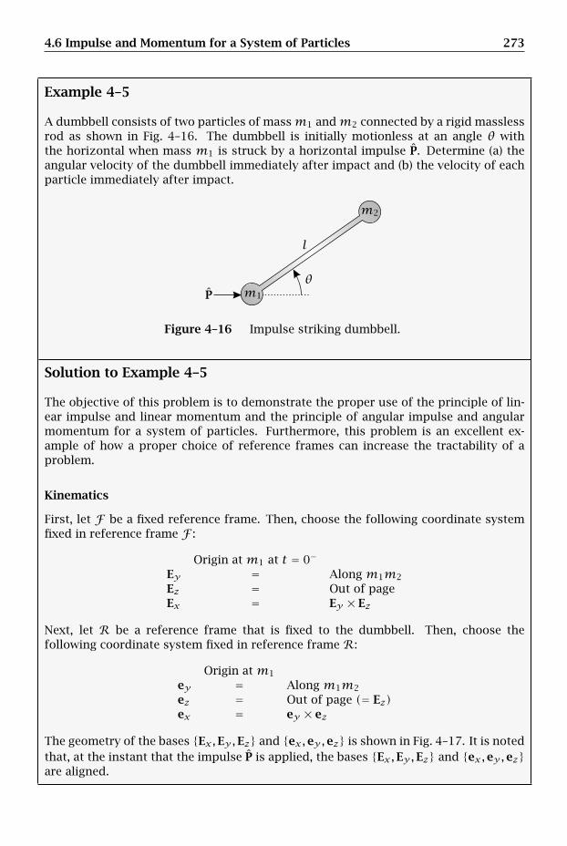
4.6 Impulse and Momentum for a System of Particles 273
Example 4–5
A dumbbell consists of two particles of massm1 andm2 connected by a rigid masslessrod as shown in Fig. 4–16. The dumbbell is initially motionless at an angle θ withthe horizontal when mass m1 is struck by a horizontal impulse P. Determine (a) theangular velocity of the dumbbell immediately after impact and (b) the velocity of eachparticle immediately after impact.
P
l
m1
m2
θ
Figure 4–16 Impulse striking dumbbell.
Solution to Example 4–5
The objective of this problem is to demonstrate the proper use of the principle of lin-ear impulse and linear momentum and the principle of angular impulse and angularmomentum for a system of particles. Furthermore, this problem is an excellent ex-ample of how a proper choice of reference frames can increase the tractability of aproblem.
Kinematics
First, let F be a fixed reference frame. Then, choose the following coordinate systemfixed in reference frame F :
Origin at m1 at t = 0−
Ey = Along m1m2
Ez = Out of pageEx = Ey × Ez
Next, let R be a reference frame that is fixed to the dumbbell. Then, choose thefollowing coordinate system fixed in reference frame R:
Origin at m1
ey = Along m1m2
ez = Out of page (= Ez)ex = ey × ez
The geometry of the bases Ex,Ey,Ez and ex,ey,ez is shown in Fig. 4–17. It is notedthat, at the instant that the impulse P is applied, the bases Ex,Ey,Ez and ex,ey,ezare aligned.
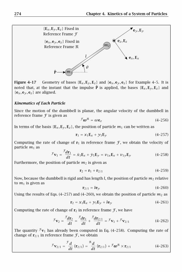
274 Chapter 4. Kinetics of a System of Particles
Ex,Ey,Ez Fixed in
ex,ey,ez Fixed in
Reference Frame F
Reference Frame Rez,Ez
ex,Ex
ey,Ey
P
l
m1
m2
θ
Figure 4–17 Geometry of bases Ex,Ey,Ez and ex,ey,ez for Example 4–5. It isnoted that, at the instant that the impulse P is applied, the bases Ex,Ey,Ez andex,ey,ez are aligned.
Kinematics of Each Particle
Since the motion of the dumbbell is planar, the angular velocity of the dumbbell inreference frame F is given as
FωR =ωez (4–256)
In terms of the basis Ex,Ey,Ez, the position of particle m1 can be written as
r1 = x1Ex +y1Ey (4–257)
Computing the rate of change of r1 in reference frame F , we obtain the velocity ofparticle m1 as
Fv1 =Fdr1
dt= x1Ex + y1Ey = v1xEx + v1yEy (4–258)
Furthermore, the position of particle m2 is given as
r2 = r1 + r2/1 (4–259)
Now, because the dumbbell is rigid and has length l, the position of particlem2 relativeto m1 is given as
r2/1 = ley (4–260)
Using the results of Eqs. (4–257) and (4–260), we obtain the position of particle m2 as
r2 = x1Ex +y1Ey + ley (4–261)
Computing the rate of change of r2 in reference frame F , we have
Fv2 =Fdr2
dt=Fdr1
dt+Fdr2/1
dt= Fv1 + Fv2/1 (4–262)
The quantity Fv1 has already been computed in Eq. (4–258). Computing the rate ofchange of r2/1 in reference frame F , we obtain
Fv2/1 =Fddt
(r2/1
) = Rddt
(r2/1
)+ FωR × r2/1 (4–263)
4.6 Impulse and Momentum for a System of Particles 275
Now we have
Rddt
(r2/1
) = 0 (4–264)
FωR × r2/1 = ωez × ley = −lωex (4–265)
Adding Eqs. (4–264) and (4–265), we obtain Fv2/1 as
Fv2/1 = −lωex (4–266)
Then, adding Eqs. (4–258) and (4–266), the velocity of particle m2 in reference frameF is given as
Fv2 = Fv1 + Fv2/1 = v1xEx + v1yEy − lωex (4–267)
Kinematics of Center of Mass of Dumbbell
The position of the center of mass of the dumbbell is given as
r = m1r1 +m2r2
m1 +m2(4–268)
Substituting the expressions for r1 and r2 from Eqs. (4–257) and (4–261), respectively,we obtain r as
r = m1(x1Ex +y1Ey)+m2(x1Ex +y1Ey + ley)m1 +m2
= x1Ex +y1Ey + m2
m1 +m2ley
(4–269)
The velocity of the center of mass of the dumbbell in reference frame F is then givenas
Fv = m1Fv1 +m2
Fv2
m1 +m2(4–270)
Substituting the expressions for Fv1 and Fv2 from Eqs. (4–258) and (4–266), respec-tively, we obtain the velocity of the center of mass of the dumbbell in reference frameF as
Fv = m1(v1xEx + v1yEy)+m2(v1xEx + v1yEy − lωey)m1 +m2
= v1xEx + v1yEy − m2
m1 +m2lωex
(4–271)
Kinematics Relative to Center of Mass of Dumbbell
For this problem the important kinematic quantities relative to the center of mass ofthe dumbbell are the position and velocity of each particle and the angular momen-tum. Using the expressions for r1, r2, and r from Eqs. (4–257), (4–261), and (4–269),respectively, we have
r1 − r = x1Ex +y1Ey −(x1Ex +y1Ey + m2
m1 +m2ley
)
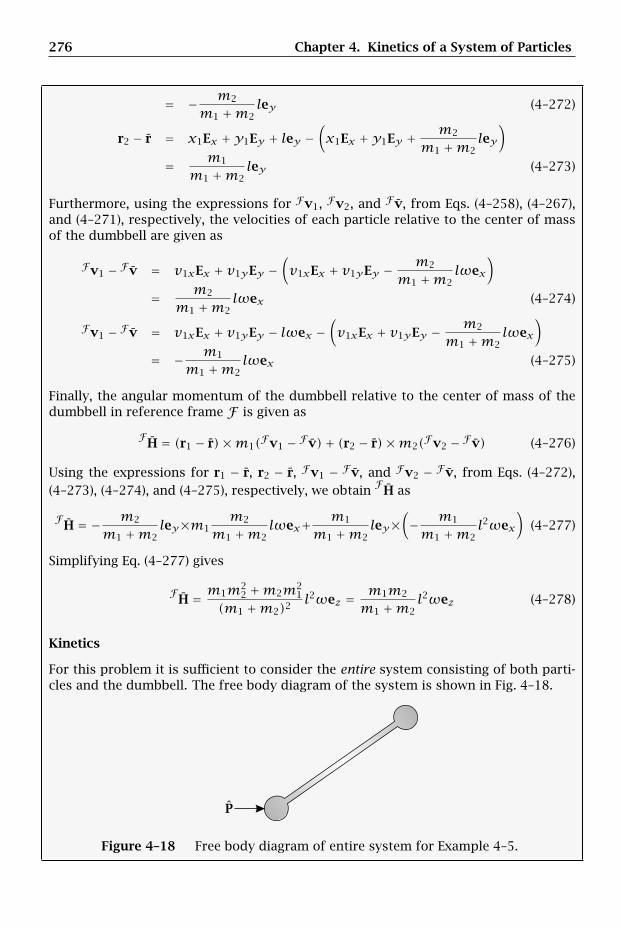
276 Chapter 4. Kinetics of a System of Particles
= − m2
m1 +m2ley (4–272)
r2 − r = x1Ex +y1Ey + ley −(x1Ex +y1Ey + m2
m1 +m2ley
)
= m1
m1 +m2ley (4–273)
Furthermore, using the expressions for Fv1, Fv2, and Fv, from Eqs. (4–258), (4–267),and (4–271), respectively, the velocities of each particle relative to the center of massof the dumbbell are given as
Fv1 − Fv = v1xEx + v1yEy −(v1xEx + v1yEy − m2
m1 +m2lωex
)
= m2
m1 +m2lωex (4–274)
Fv1 − Fv = v1xEx + v1yEy − lωex −(v1xEx + v1yEy − m2
m1 +m2lωex
)
= − m1
m1 +m2lωex (4–275)
Finally, the angular momentum of the dumbbell relative to the center of mass of thedumbbell in reference frame F is given as
FH = (r1 − r)×m1(Fv1 − Fv)+ (r2 − r)×m2(Fv2 − Fv) (4–276)
Using the expressions for r1 − r, r2 − r, Fv1 − Fv, and Fv2 − Fv, from Eqs. (4–272),(4–273), (4–274), and (4–275), respectively, we obtain
FH as
FH = − m2
m1 +m2ley×m1
m2
m1 +m2lωex+ m1
m1 +m2ley×
(− m1
m1 +m2l2ωex
)(4–277)
Simplifying Eq. (4–277) gives
FH = m1m2
2 +m2m21
(m1 +m2)2l2ωez = m1m2
m1 +m2l2ωez (4–278)
Kinetics
For this problem it is sufficient to consider the entire system consisting of both parti-cles and the dumbbell. The free body diagram of the system is shown in Fig. 4–18.
P
Figure 4–18 Free body diagram of entire system for Example 4–5.
4.6 Impulse and Momentum for a System of Particles 277
It is seen that the only external impulse acting on the system is P. Resolving theimpulse P in the basis Ex,Ey,Ez, we obtain
P = P sinθEx + P cosθEy (4–279)
Now for this problem we need to apply both the principle of linear impulse and mo-mentum and the principle of angular impulse and momentum.
Application of Linear Impulse and Linear Momentum to Dumbbell
Applying the principle of linear impulse and linear momentum to the entire system inreference frame F , we have
F = FG′ − FG (4–280)
where FG and FG′ are the linear momenta of the system the instants before and afterthe application of P, respectively. Now it is seen that P is the only impulse acting onthe system. Using the expression for P from Eq. (4–279), we have
F = P = P sinθEx + P cosθEy (4–281)
Furthermore, because the dumbbell is at rest before P is applied, we have
FG = 0 (4–282)
Finally, the linear momentum of the system immediately after the impulse P is appliedis given as
FG′ =mFv′ = (m1 +m2)Fv′ (4–283)
where Fv′ is the velocity of the center of mass in reference frame F immediately afterP is applied. Then, using the expression for Fv′ from Eq. (4–271), we obtain FG′ as
FG′ = (m1 +m2)(v′1xEx + v′1yEy − m2
m1 +m2lω′ex
)(4–284)
Rewriting Eq. (4–284), we obtain
FG′ = (m1 +m2)v′1xEx + (m1 +m2)v′1yEy −m2lω′ex (4–285)
Because ex and Ex are aligned at the instant the impulse P is applied, Eq. (4–285)simplifies to
FG′ = [(m1 +m2)v′1x −m2lω′]Ex + (m1 +m2)v′1yEy (4–286)
Substituting FG′ from Eq. (4–286) and F from Eq. (4–281) into (4–280), we obtain
P sinθEx + P cosθEy =[(m1 +m2)v′1x −m2lω′]Ex + (m1 +m2)v′1yEy (4–287)
Equating components in Eq. (4–287), we obtain the following two scalar equations:
P sinθ = (m1 +m2)v′1x −m2lω′ (4–288)
P cosθ = (m1 +m2)v′1y (4–289)
278 Chapter 4. Kinetics of a System of Particles
Application of Angular Impulse and Angular Momentum to Dumbbell
For this problem it is convenient to apply angular impulse and angular momentum inreference frame F relative to the center of mass of the dumbbell. Consequently, wehave
ˆM = FH′ − F
H (4–290)
Because the only impulse applied to the dumbbell is P and P is applied at the locationof particle m1, the angular impulse applied to the dumbbell relative to the center ofmass of the dumbbell is given as
ˆM = (r1 − r)× P (4–291)
Using the expressions for r1 − r and P from Eqs. (4–272) and (4–279), respectively, weobtain ˆM as
ˆM = − m2
m1 +m2ley × (P sinθEx + P cosθEy) (4–292)
However, because ey and Ey are aligned at the instant that P is applied, the angularimpulse applied relative to the center of mass of the dumbbell simplifies to
ˆM = − m2
m1 +m2lEy × (P sinθEx + P cosθEy)
= m2
m1 +m2lP sinθEz = m2
m1 +m2lP sinθez
(4–293)
Next, because the dumbbell is at rest the instant before the impulse P is applied, wehave
FH = 0 (4–294)
Furthermore, using the expression forF
H from Eq. (4–278), the angular momentum ofthe dumbbell relative to the center of mass of the dumbbell in reference frame F theinstant after the impulse P is applied is given as
FH′ = m1m2
m1 +m2l2ω′ez (4–295)
Setting the results of Eqs. (4–293) and (4–295) equal, we obtain
m2
m1 +m2lP sinθez = m1m2
m1 +m2l2ω′ez (4–296)
Simplifying Eq. (4–296) gives
ω′ = P sinθm1l
(4–297)
(a) Determination of Angular Velocity of Dumbbell the Instant After P Is Applied
The angular velocity of the dumbbell the instant after P is applied is obtained directlyfrom Eq. (4–297) and is given as
(FωR
)′ =ω′ez = P sinθm1l
ez (4–298)
4.6 Impulse and Momentum for a System of Particles 279
(b) Determination of Velocity of Each Particle the Instant After P Is Applied
The velocities of each particle in reference frame F the instant after the impulse P isapplied are obtained using Eqs. (4–288), (4–289), and (4–297. Substituting the result ofEq. (4–297) into (4–288), we obtain
P sinθ = (m1 +m2)v′1x −m2lP sinθm1l
(4–299)
Rearranging Eq. (4–299), we obtain
(m1 +m2)v′1x =(
1+ m2
m1
)P sinθ (4–300)
Equation (4–300) can be rewritten as
(m1 +m2)v′1x =m1 +m2
m1P sinθ (4–301)
Solving Eq. (4–301) for v′1x , we obtain
v′1x =P sinθm1
(4–302)
Next, solving Eq. (4–289) for v′1y gives
v′1y =P cosθm1 +m2
(4–303)
Substituting the results of Eqs. (4–302) and (4–303) into Eq. (4–258), we obtain thevelocity of particle m1 in reference frame F the instant after the impulse P is appliedas
Fv′1 =P sinθm1
Ex + P cosθm1 +m2
Ey (4–304)
Then, substituting the results of Eqs. (4–297), (4–302), and (4–303) into Eq. (4–267), weobtain the velocity of particle m2 in reference frame F the instant after the impulse Pis applied as
Fv′2 =P sinθm1
Ex + P cosθm1 +m2
Ey − P sinθm1
ex (4–305)
Finally, because the directions ex and Ex are aligned at the instant that the impulse Pis applied, Eq. (4–305) simplifies to
Fv′2 =P cosθm1 +m2
Ey (4–306)
280 Chapter 4. Kinetics of a System of Particles
4.7 Work and Energy for a System of Particles
4.7.1 Kinetic Energy for a System of Particles
The kinetic energy for a system of particles in an inertial reference frame N is definedas
NT = 12
n∑i=1
miNvi · Nvi (4–307)
An alternate expression for the kinetic energy is obtained as follows. First, we have
Nvi = Nvi −Nv+Nv (4–308)
where it is noted in Eq. (4–308) that the velocity of the center of mass of the system,Nv, has merely been added and subtracted. Substituting Eq. (4–308) into (4–307), weobtain
NT = 12
n∑i=1
mi
(Nvi −Nv+Nv
)·(Nvi −Nv+Nv
)(4–309)
Expanding Eq. (4–309) gives
NT = 12
⎡⎣ n∑i=1
mi
(Nvi −Nv
)·(Nvi −Nv
)+
n∑i=1
mi
(Nvi −Nv
)· Nv
+n∑i=1
mi
(Nvi −Nv
)· Nv+
n∑i=1
miNv · Nv
⎤⎦
(4–310)
Combining the second and third terms in Eq. (4–310), we obtain
NT = 12
⎡⎣ n∑i=1
mi
(Nvi −Nv
)·(Nvi −Nv
)
+2n∑i=1
mi
(Nvi −Nv
)· Nv+
n∑i=1
miNv · Nv
⎤⎦
(4–311)
Because Nv is independent of the summation, we have
n∑i=1
miNv · Nv =mNv · Nv (4–312)
Furthermore,
n∑i=1
mi
(Nvi −Nv
)=
n∑i=1
miNvi −
n∑i=1
miNv =mNv−mNv = 0 (4–313)
The kinetic energy of Eq. (4–311) then simplifies to
NT = 12mNv · Nv+ 1
2
n∑i=1
mi
(Nvi −Nv
)·(Nvi −Nv
)(4–314)
4.7 Work and Energy for a System of Particles 281
For compactness we can write
NT = NT(1) +NT(2) (4–315)
where
NT(1) = 12m
Nv · Nv (4–316)
NT(2) = 12
n∑i=1
mi
(Nvi −Nv
)·(Nvi −Nv
)(4–317)
Equation (4–314) is called Koenig’s decomposition and states that the kinetic energy ofa system of particles, NT , is equal to the sum of the kinetic energy of the center ofmass of the system, NT(1), and the kinetic energy relative to the center of mass of thesystem, NT(2).
4.7.2 Work-Energy Theorem for a System of Particles
Computing the rate of change of NT(1) as given in Eq. (4–316), we have
ddt
(NT(1)
)= 1
2m[Na · Nv+Nv · Na
](4–318)
Using the fact that the scalar product is commutative, Eq. (4–318) simplifies to
ddt
(NT(1)
)=mNa · Nv (4–319)
Then, substituting the result of Eq. (4–38) into (4–319), we have
ddt
(NT(1)
)= F · Nv = NP(1) (4–320)
Equation (4–320) states that the power of all external forces acting on a system ofparticles is equal to the rate of change of the kinetic energy of the center of mass ofthe system. Integrating Eq. (4–320) from time t = t1 to t = t2, we have
∫ t2t1
ddt
(NT(1)
)dt =
∫ t2t1
F · Nvdt (4–321)
Now it can be seen that the left-hand side of Eq. (4–321) is equal to NT(1)2 − NT(1)1 .Furthermore, it is seen that ∫ t2
t1F · Nvdt
is the work done by all of the external forces on the time interval t ∈ [t1, t2]. Conse-quently, Eq. (4–321) can be written as
NT(1)(t2)−NT(1)(t1) = NW(1)12 (4–322)
Equation (4–322) states that the work done by all external forces acting on a system inmoving the center of mass of the system over a time interval t ∈ [t1, t2] is equal to thechange in the kinetic energy associated with the center of mass of the system.
282 Chapter 4. Kinetics of a System of Particles
Next, computing the rate of change of the total kinetic energy NT , we have
ddt
(NT
)= 1
2m[Na · Nv+Nv · Na
]
+ 12
n∑i=1
mi
[(Nai −Na
)·(Nvi −Nv
)+(Nvi −Nv
)·(Nai −Na
)] (4–323)
Using the fact that the scalar product is commutative, Eq. (4–323) simplifies to
ddt
(NT
)=mNa · Nv+
n∑i=1
mi
(Nai −Na
)·(Nvi −Nv
)(4–324)
Equation (4–324) can be rewritten as
ddt
(NT
)=mNa · Nv+
n∑i=1
miNai ·
(Nvi −Nv
)−
n∑i=1
miNa ·
(Nvi −Nv
)(4–325)
Substituting the result of Eq. (4–32) into (4–325) and noting that Na is independent ofthe summation, we obtain
ddt
(NT
)= F · Nv+
n∑i=1
Ri ·(Nvi −Nv
)−Na ·
n∑i=1
mi
(Nvi −Nv
)(4–326)
From the definition of the center of mass, we have
n∑i=1
mi
(Nvi −Nv
)= 0 (4–327)
Consequently, Eq. (4–326) simplifies to
ddt
(NT
)= F · Nv+
n∑i=1
Ri ·(Nvi −Nv
)(4–328)
Furthermore, we have
n∑i=1
Ri · Nv = Nv ·n∑i=1
Ri = Nv ·n∑i=1
⎡⎣Fi +
n∑j=1
fij
⎤⎦ = Nv ·
n∑i=1
Fi = F · Nv (4–329)
Therefore, Eq. (4–328) reduces to
ddt
(NT
)=
n∑i=1
Ri · Nvi (4–330)
Equation (4–330) is the work-energy theorem for a system of particles and states thatthe rate of change of kinetic energy of a system of particles is equal to the powerproduced by all internal and external forces acting on the system.
4.7 Work and Energy for a System of Particles 283
4.7.3 Alternate Form of Work-Energy Theorem for a System of Particles
Suppose now that the external force applied to each particle in the system is decom-posed as
Fi = Fci + Fnci (i = 1, . . . , n) (4–331)
whereFci = External conservative force applied to particle i
Fnci = External nonconservative force applied to particle i
Then the resultant force acting on particle i can be written as
Ri = Fci + Fnci +n∑j=1
fij (i = 1, . . . , n) (4–332)
Substituting the result of Eq. (4–332) into the work-energy theorem of Eq. (4–330), weobtain
ddt
(NT
)=
n∑i=1
⎡⎣Fci + Fnci +
n∑j=1
fij
⎤⎦ · Nvi (4–333)
Expanding Eq. (4–333) gives
ddt
(NT
)=
n∑i=1
Fci · Nvi +n∑i=1
⎡⎣Fnci +
n∑j=1
fij
⎤⎦ · Nvi (4–334)
Now, because the forces Fci , (i = 1, . . . , n) are conservative, we know that there existpotential energy functions NUi, (i = 1, . . . , n) such that
Fci · Nvi = − ddt(NUi
)(i = 1, . . . , n) (4–335)
Using the result of Eq. (4–335) in (4–334), we have
ddt
(NT
)= −
n∑i=1
ddt
(NUi
)+
n∑i=1
⎡⎣Fnci +
n∑i=1
n∑j=1
fij
⎤⎦ · Nvi (4–336)
Suppose now that we let the resultant nonconservative force acting on particle i, (i =1, . . . , n) be defined as
Rnci = Fnci +n∑j=1
fij (4–337)
Equation (4–336) can then be written as
ddt
(NT
)= −
n∑i=1
ddt
(NUi
)+
n∑i=1
Rnci · Nvi (4–338)
where the quantityn∑i=1
Rnci · Nvi (4–339)
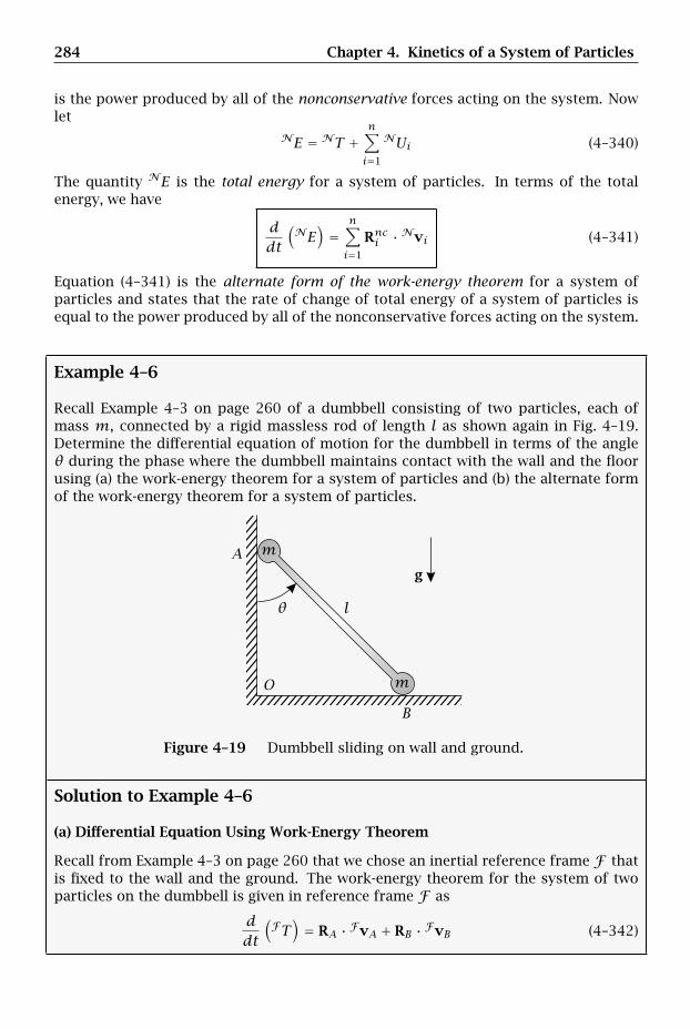
284 Chapter 4. Kinetics of a System of Particles
is the power produced by all of the nonconservative forces acting on the system. Nowlet
NE = NT +n∑i=1
NUi (4–340)
The quantity NE is the total energy for a system of particles. In terms of the totalenergy, we have
ddt
(NE
)=
n∑i=1
Rnci · Nvi (4–341)
Equation (4–341) is the alternate form of the work-energy theorem for a system ofparticles and states that the rate of change of total energy of a system of particles isequal to the power produced by all of the nonconservative forces acting on the system.
Example 4–6
Recall Example 4–3 on page 260 of a dumbbell consisting of two particles, each ofmass m, connected by a rigid massless rod of length l as shown again in Fig. 4–19.Determine the differential equation of motion for the dumbbell in terms of the angleθ during the phase where the dumbbell maintains contact with the wall and the floorusing (a) the work-energy theorem for a system of particles and (b) the alternate formof the work-energy theorem for a system of particles.
g
l
m
mA
B
O
θ
Figure 4–19 Dumbbell sliding on wall and ground.
Solution to Example 4–6
(a) Differential Equation Using Work-Energy Theorem
Recall from Example 4–3 on page 260 that we chose an inertial reference frame F thatis fixed to the wall and the ground. The work-energy theorem for the system of twoparticles on the dumbbell is given in reference frame F as
ddt
(FT
)= RA · FvA + RB · FvB (4–342)
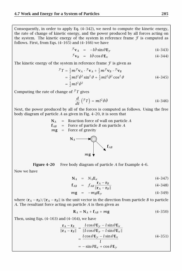
4.7 Work and Energy for a System of Particles 285
Consequently, in order to apply Eq. (4–342), we need to compute the kinetic energy,the rate of change of kinetic energy, and the power produced by all forces acting onthe system. The kinetic energy of the system in reference frame F is computed asfollows. First, from Eqs. (4–165) and (4–166) we have
FvA = −lθ sinθEy (4–343)FvB = lθ cosθEx (4–344)
The kinetic energy of the system in reference frame F is given as
FT = 12m
FvA · FvA + 12m
FvB · FvB
= 12ml
2θ2 sin2θ + 12ml
2θ2 cos2θ
= 12ml
2θ2
(4–345)
Computing the rate of change of FT gives
ddt
(FT
)=ml2θθ (4–346)
Next, the power produced by all of the forces is computed as follows. Using the freebody diagram of particle A as given in Fig. 4–20, it is seen that
NA = Reaction force of wall on particle AfAB = Force of particle B on particle Amg = Force of gravity
NA
fAB
mg
Figure 4–20 Free body diagram of particle A for Example 4–6.
Now we have
NA = NAEx (4–347)
fAB = fABrA − rB‖rA − rB‖
(4–348)
mg = −mgEy (4–349)
where (rA − rB)/‖rA − rB‖ is the unit vector in the direction from particle B to particleA. The resultant force acting on particle A is then given as
RA = NA + fAB +mg (4–350)
Then, using Eqs. (4–163) and (4–164), we have
rA − rB‖rA − rB‖
= l cosθEy − l sinθEx‖l cosθEy − l sinθEx‖
= l cosθEy − l sinθExl
= − sinθEx + cosθEy
(4–351)
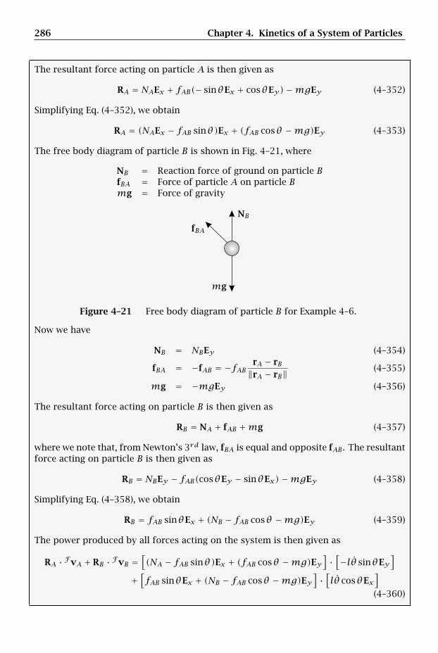
286 Chapter 4. Kinetics of a System of Particles
The resultant force acting on particle A is then given as
RA = NAEx + fAB(− sinθEx + cosθEy)−mgEy (4–352)
Simplifying Eq. (4–352), we obtain
RA = (NAEx − fAB sinθ)Ex + (fAB cosθ −mg)Ey (4–353)
The free body diagram of particle B is shown in Fig. 4–21, where
NB = Reaction force of ground on particle BfBA = Force of particle A on particle Bmg = Force of gravity
NB
fBA
mg
Figure 4–21 Free body diagram of particle B for Example 4–6.
Now we have
NB = NBEy (4–354)
fBA = −fAB = −fAB rA − rB‖rA − rB‖
(4–355)
mg = −mgEy (4–356)
The resultant force acting on particle B is then given as
RB = NA + fAB +mg (4–357)
where we note that, from Newton’s 3rd law, fBA is equal and opposite fAB . The resultantforce acting on particle B is then given as
RB = NBEy − fAB(cosθEy − sinθEx)−mgEy (4–358)
Simplifying Eq. (4–358), we obtain
RB = fAB sinθEx + (NB − fAB cosθ −mg)Ey (4–359)
The power produced by all forces acting on the system is then given as
RA · FvA + RB · FvB =[(NA − fAB sinθ)Ex + (fAB cosθ −mg)Ey
]·[−lθ sinθEy
]+[fAB sinθEx + (NB − fAB cosθ −mg)Ey
]·[lθ cosθEx
](4–360)
4.7 Work and Energy for a System of Particles 287
Simplifying Eq. (4–360), we have
RA · FvA + RB · FvB = −fABlθ cosθ sinθ +mglθ sinθ + fABlθ sinθ cosθ
=mglθ sinθ(4–361)
Setting the rate of change of kinetic energy as given in Eq. (4–346) equal to the powerproduced by all forces as given in Eq. (4–361), we obtain
ml2θθ =mglθ sinθ (4–362)
Rearranging Eq. (4–362), we obtain
θ(ml2θ −mgl sinθ) = 0 (4–363)
Since θ ≠ 0 as a function of time (otherwise the dumbbell would not move), we have
ml2θ −mgl sinθ = 0 (4–364)
Simplifying Eq. (4–364), the differential equation of motion is obtained as
θ − gl
sinθ = 0 (4–365)
It is observed that the result of Eq. (4–365) is identical to that obtained in Eq. (4–196)on page 264 of Example 4–3.
(b) Differential Equation Using Alternate Form of Work-Energy Theorem
For this problem the alternate form of the work-energy theorem is given in referenceframe F as
ddt
(FE)= RncA · FvA + RncB · FvB (4–366)
where RncA and RncB are the resultant nonconservative forces acting on particles A andB, respectively. First, the total energy is given as
FE = FT + FU (4–367)
We already have the kinetic energy from Eq. (4–345). Next, because the only conserva-tive force acting on the dumbbell is that of gravity, the potential energy in referenceframe F is given as
FU = FUg = −2mg · r (4–368)
Recalling the position of the center of mass of the dumbbell and the force due togravity from Eqs. (4–170) and (4–181) on pages 261 and 263, respectively, we have
FU = −(−2mgEy) ·(l2 sinθEx + l
2 cosθEy)=mgl cosθ (4–369)
Then, adding Eqs. (4–345) and (4–369), the total energy is given as
FE = 12ml
2θ2 +mgl cosθ (4–370)
288 Chapter 4. Kinetics of a System of Particles
Computing the rate of change of the total energy, we obtain
ddt
(FE)=ml2θθ −mglθ sinθ (4–371)
Now the nonconservative force acting on particle A is given as
RncA = NA + fAB (4–372)
where NA is the force exerted by the vertical wall and fAB is the force exerted by particleB. Using the expressions for NA and fAB from Eqs. (4–347) and (4–348), respectively,we obtain
RncA = NAEx + fAB rA − rB‖rA − rB‖
(4–373)
Using the expression for (rA − rB)/‖rA − rB‖ from Eq. (4–351), we have
RncA = NAEx + fAB(− sinθEx + cosθEy) = (NA − fAB sinθ)Ex + fAB cosθEy (4–374)
Similarly, the nonconservative force acting on particle B is given as
RncB = NB + fBA (4–375)
where NB is the force exerted by the vertical wall and fBA is the force exerted by particleA. Using the expressions for NB and fBA from Eqs. (4–354) and (4–355), respectively,we obtain
RncB = NBEy − fAB rA − rB‖rA − rB‖
(4–376)
Again, using the expression for (rA − rB)/‖rA − rB‖ from Eq. (4–351), we have
RncB = NBEy − fAB(− sinθEx + cosθEy) = fAB sinθ + (NB − fAB cosθ)Ey (4–377)
Then, using the expressions for FvA and FvB from Eqs. (4–343) and (4–344), the powerproduced by all nonconservative forces is given as
RncA · FvA + RncB · FvB =[(NA − fAB sinθ)Ex + fAB cosθEy
]·[−lθ sinθEy
]+[fAB sinθEx + (NB − fAB cosθ)Ey
]·[lθ cosθEx
]= −fABlθ cosθ sinθ + fABlθ sinθ cosθ = 0
(4–378)
It is noted that Eq. (4–371) implies that the total energy in reference frame F is con-served. Setting the rate of change of total energy in Eq. (4–371) equal to the powerproduced by all nonconservative forces in Eq. (4–378, we obtain
ml2θθ −mglθ sinθ = 0 (4–379)
Noting that θ cannot be zero as a function of time (otherwise the dumbbell would notmove), we have
ml2θ −mgl sinθ = 0 (4–380)
Simplifying Eq. (4–380), we obtain the differential equation of motion as
θ − gl
sinθ = 0 (4–381)
It is observed that the result of Eq. (4–381) is identical to that obtained in Eq. (4–365)using the work-energy theorem and is also identical to the result obtained in Eq. (4–196) on page 264 of Example 4–3.

4.8 Collision of Particles 289
4.8 Collision of Particles
A collision is defined as the impact between two objects that occurs over a very shortduration of time and where the forces exerted by each object on the other are ex-tremely large.3 It can be seen that a real collision can be difficult to model becausetwo real physical objects are generally oddly shaped, are generally composed of non-homogeneous materials, and occupy a nonzero amount of space. Consequently, thedeformations that real physical objects undergo during a collision are highly nontriv-ial. However, by making an appropriate set of assumptions and simplifications, it ispossible to arrive at a representative model to express the post-collision velocities oftwo bodies in terms of the pre-collision velocities of the bodies. In particular, a com-monly used collision model is obtained by making the following assumptions: (1) thecollision occurs over a very short time interval, and, thus, the positions of the bodiesdo not change during the collision; (2) the colliding bodies are either particles (i.e., thebodies occupy no physical space) or are homogeneous spheres (so that the directionalong which the collision takes place passes through the geometric centers of the bod-ies), and, thus, the impact is a central impact;4 (3) The surfaces of the objects are“smooth,” and, thus there is no friction between the particles during the collision; (4)The kinetics associated with the deformations of the bodies are lumped into an ad hocscalar parameter called the coefficient of restitution. Using these assumptions, a modelfor the collision between two particles is now developed. It is noted that the devel-opment of this section is functionally similar to that found in many other dynamicsbooks, including Beer and Johnston (1997), Hibbeler (2001), Greenwood (1988), andO’Reilly (2001).
Let P1 and P2 be particles of mass m1 and m2, respectively, moving in an inertialreference frame N . Furthermore, assume that P1 and P2 are following independenttrajectories in reference frame N when the paths of the particles coincide, therebyresulting in a collision. The geometry of the collision is shown in Fig. 4–22.It is evident that the collision will change the velocity of each particle in a mannerdifferent from the change that would have occurred had the particles not collided. Inorder to determine the effect that the collision has on the velocity of each particle,we focus on the interval of time over which the collision occurs. In particular, duringthe collision it is assumed that there exists a well-defined tangent plane, TP , to thesurface of each particle at the point of contact, P . The impact is assumed to occurin a direction n that is normal to TP . The direction n is referred to as the direction ofimpact or the line of impact (Beer and Johnston, 1997; Bedford and Fowler, 2005). Also,in order to describe motion in the tangent plane TP ,we define two unit vectors u andw whose directions lie in TP during the collision (Greenwood, 1988; O’Reilly, 2001). Itis assumed that the vectors n, u, and w are constant during the collision and that uand w are chosen such that u,w,n forms a right-handed system (Greenwood, 1988;O’Reilly, 2001).
3The terms “collision” and “impact” are, generally speaking, used interchangeably.4In many dynamics books (e.g., Beer and Johnston (1997) and Bedford and Fowler (2005)), the derivation
of collision of particles is divided into two parts, commonly referred to as direct central impact and obliquecentral impact. However, direct central impact is a special case of oblique central impact and need not beconsidered separately. In the development presented here, we discuss the general case of oblique centralimpact and use the general term central impact. Finally, it is noted that all of the results presented herecan be applied to the special case of direct central impact.
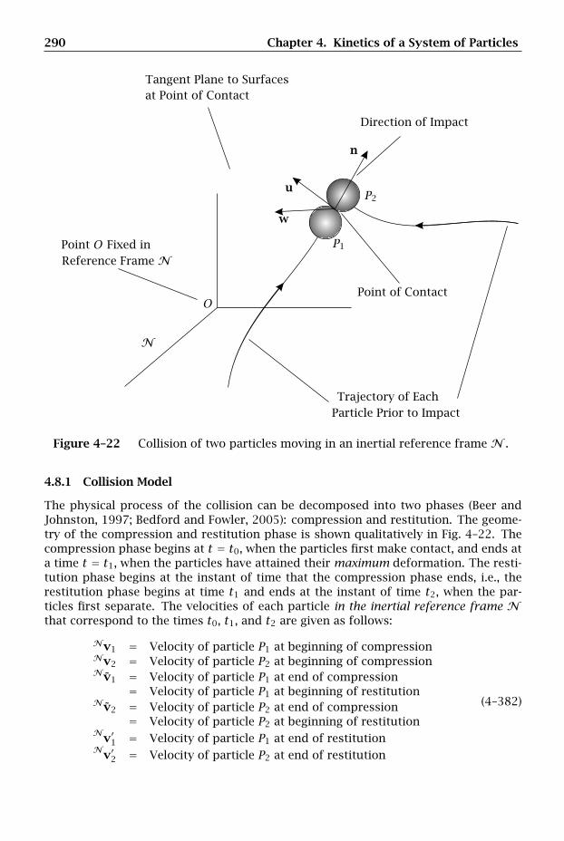
290 Chapter 4. Kinetics of a System of Particles
Point of Contact
Tangent Plane to Surfacesat Point of Contact
Direction of Impact
Trajectory of EachParticle Prior to Impact
Point O Fixed in
N
Reference Frame N
n
u
w
O
P1
P2
Figure 4–22 Collision of two particles moving in an inertial reference frame N .
4.8.1 Collision Model
The physical process of the collision can be decomposed into two phases (Beer andJohnston, 1997; Bedford and Fowler, 2005): compression and restitution. The geome-try of the compression and restitution phase is shown qualitatively in Fig. 4–22. Thecompression phase begins at t = t0, when the particles first make contact, and ends ata time t = t1, when the particles have attained their maximum deformation. The resti-tution phase begins at the instant of time that the compression phase ends, i.e., therestitution phase begins at time t1 and ends at the instant of time t2, when the par-ticles first separate. The velocities of each particle in the inertial reference frame Nthat correspond to the times t0, t1, and t2 are given as follows:
Nv1 = Velocity of particle P1 at beginning of compressionNv2 = Velocity of particle P2 at beginning of compressionNv1 = Velocity of particle P1 at end of compression
= Velocity of particle P1 at beginning of restitutionNv2 = Velocity of particle P2 at end of compression
= Velocity of particle P2 at beginning of restitutionNv′1 = Velocity of particle P1 at end of restitutionNv′2 = Velocity of particle P2 at end of restitution
(4–382)
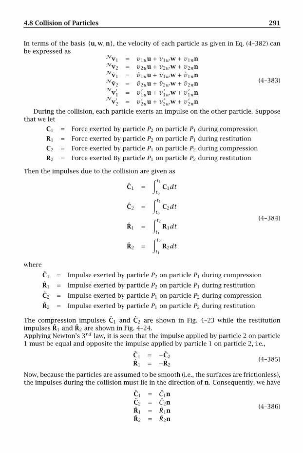
4.8 Collision of Particles 291
In terms of the basis u,w,n, the velocity of each particle as given in Eq. (4–382) canbe expressed as
Nv1 = v1uu+ v1ww+ v1nnNv2 = v2uu+ v2ww+ v2nnNv1 = v1uu+ v1ww+ v1nnNv2 = v2uu+ v2ww+ v2nnNv′1 = v′1uu+ v′1ww+ v′1nnNv′2 = v′2uu+ v′2ww+ v′2nn
(4–383)
During the collision, each particle exerts an impulse on the other particle. Supposethat we let
C1 = Force exerted by particle P2 on particle P1 during compression
R1 = Force exerted by particle P2 on particle P1 during restitution
C2 = Force exerted by particle P1 on particle P2 during compression
R2 = Force exerted By particle P1 on particle P2 during restitution
Then the impulses due to the collision are given as
C1 =∫ t1t0
C1dt
C2 =∫ t1t0
C2dt
R1 =∫ t2t1
R1dt
R2 =∫ t2t1
R2dt
(4–384)
where
C1 = Impulse exerted by particle P2 on particle P1 during compression
R1 = Impulse exerted by particle P2 on particle P1 during restitution
C2 = Impulse exerted by particle P1 on particle P2 during compression
R2 = Impulse exerted by particle P1 on particle P2 during restitution
The compression impulses C1 and C2 are shown in Fig. 4–23 while the restitutionimpulses R1 and R2 are shown in Fig. 4–24.Applying Newton’s 3rd law, it is seen that the impulse applied by particle 2 on particle1 must be equal and opposite the impulse applied by particle 1 on particle 2, i.e.,
C1 = −C2
R1 = −R2(4–385)
Now, because the particles are assumed to be smooth (i.e., the surfaces are frictionless),the impulses during the collision must lie in the direction of n. Consequently, we have
C1 = C1nC2 = C2nR1 = R1nR2 = R2n
(4–386)

292 Chapter 4. Kinetics of a System of Particles
Direction of Impact
C1
C2
n
u
w
P1
P2
Figure 4–23 Free body diagram during compression phase of the collision betweentwo particles.
Direction of Impact
R1
R2
n
u
w
P1
P2
Figure 4–24 Free body diagram during restitution phase of the collision betweentwo particles.
Furthermore, it is assumed that, during the collision of the two particles, all otherimpulses are negligible in comparison to the C1, C2, R1, and R2. Using the impulsesgiven in Eq. (4–386), we define the scalar parameter e called the coefficient of restitutionas
e = R1 · n
C1 · n= R2 · n
C2 · n(4–387)
Finally, using Eq. (4–387), we can solve for R1 ·n and R2 ·n in terms of C1 ·n and C2 ·nas
R1 · n = eC1 · nR2 · n = eC2 · n
(4–388)
Application of Linear Impulse and Linear Momentum During Compression
Applying the principle of linear impulse and linear momentum of Eq. (3–179) frompage 177 to each particle during compression, we have
C1 = NG1 −NG1
C2 = NG2 −NG2
(4–389)
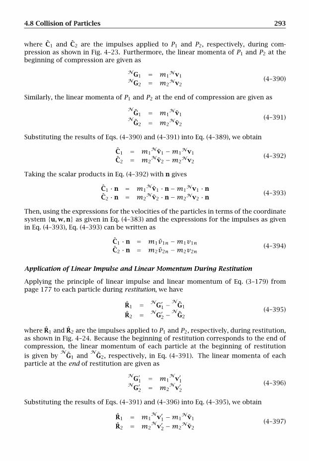
4.8 Collision of Particles 293
where C1 and C2 are the impulses applied to P1 and P2, respectively, during com-pression as shown in Fig. 4–23. Furthermore, the linear momenta of P1 and P2 at thebeginning of compression are given as
NG1 = m1Nv1
NG2 = m2Nv2
(4–390)
Similarly, the linear momenta of P1 and P2 at the end of compression are given as
NG1 = m1
Nv1N
G2 = m2Nv2
(4–391)
Substituting the results of Eqs. (4–390) and (4–391) into Eq. (4–389), we obtain
C1 = m1Nv1 −m1
Nv1
C2 = m2Nv2 −m2
Nv2(4–392)
Taking the scalar products in Eq. (4–392) with n gives
C1 · n = m1Nv1 · n−m1
Nv1 · nC2 · n = m2
Nv2 · n−m2Nv2 · n
(4–393)
Then, using the expressions for the velocities of the particles in terms of the coordinatesystem u,w,n as given in Eq. (4–383) and the expressions for the impulses as givenin Eq. (4–393), Eq. (4–393) can be written as
C1 · n = m1v1n −m1v1nC2 · n = m2v2n −m2v2n
(4–394)
Application of Linear Impulse and Linear Momentum During Restitution
Applying the principle of linear impulse and linear momentum of Eq. (3–179) frompage 177 to each particle during restitution, we have
R1 = NG′1 −N
G1
R2 = NG′2 −N
G2(4–395)
where R1 and R2 are the impulses applied to P1 and P2, respectively, during restitution,as shown in Fig. 4–24. Because the beginning of restitution corresponds to the end ofcompression, the linear momentum of each particle at the beginning of restitution
is given byN
G1 andN
G2, respectively, in Eq. (4–391). The linear momenta of eachparticle at the end of restitution are given as
NG′1 = m1Nv′1
NG′2 = m2Nv′2
(4–396)
Substituting the results of Eqs. (4–391) and (4–396) into Eq. (4–395), we obtain
R1 = m1Nv′1 −m1
Nv1
R2 = m2Nv′2 −m2
Nv2(4–397)
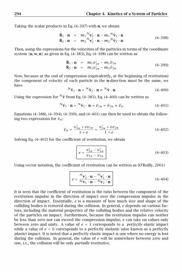
294 Chapter 4. Kinetics of a System of Particles
Taking the scalar products in Eq. (4–397) with n, we obtain
R1 · n = m1Nv′1 · n−m1
Nv1 · n
R2 · n = m2Nv′2 · n−m2
Nv2 · n(4–398)
Then, using the expressions for the velocities of the particles in terms of the coordinatesystem u,w,n as given in Eq. (4–383), Eq. (4–398) can be written as
R1 · n = m1v′1n −m1v1nR2 · n = m2v′2n −m2v2n
(4–399)
Now, because at the end of compression (equivalently, at the beginning of restitution)the component of velocity of each particle in the n-direction must be the same, wehave
Nv1 · n = Nv2 · n ≡ Nv · n (4–400)
Using the expression for Nv from Eq. (4–383), Eq. (4–400) can be written as
Nv1 · n = Nv2 · n = v1n = v2n ≡ vn (4–401)
Equations (4–388), (4–394), (4–399), and (4–401) can then be used to obtain the follow-ing two expressions for vn:
vn =v′1n + ev1n
1+ e = v′2n + ev2n
1+ e (4–402)
Solving Eq. (4–402) for the coefficient of restitution, we obtain
e = v′2n − v′1nv1n − v2n
(4–403)
Using vector notation, the coefficient of restitution can be written as (O’Reilly, 2001)
e =Nv′2 · n−Nv′1 · nNv1 · n−Nv2 · n
(4–404)
It is seen that the coefficient of restitution is the ratio between the component of therestitution impulse in the direction of impact over the compression impulse in thedirection of impact. Essentially, e is a measure of how much size and shape of thecolliding bodies is restored during the collision. In general, e depends on various fac-tors, including the material properties of the colliding bodies and the relative velocityof the particles on impact. Furthermore, because the restitution impulse can neitherbe less than zero nor can exceed the compression impulse, e can take on values onlybetween zero and unity. A value of e = 1 corresponds to a perfectly elastic impactwhile a value of e = 0 corresponds to a perfectly inelastic (also known as a perfectlyplastic) impact. It is noted that a perfectly elastic impact is one where no energy is lostduring the collision. In general, the value of e will be somewhere between zero andone, i.e., the collision will be only partially restitutive.
4.8 Collision of Particles 295
Application of Linear impulse and Linear momentum During Entire Collision
Applying the principle of linear impulse and linear momentum of Eq. (3–179) frompage 177 to each particle during the entire collision (i.e., during both compression andrestitution), we have
F1 = NG′1 −NG1
F2 = NG′2 −NG2(4–405)
where F1 and F2 are the impulses applied to P1 and P2, respectively, during the entirecollision. Now it is seen that the impulses applied to P1 and P2, respectively, duringthe entire collision are the sum of the impulses during compression and restitution,i.e.,
F1 = C1 + R1
F2 = C2 + R2(4–406)
Substituting the result of Eq. (4–406) together with the pre-collision and post-collisionlinear momenta as given, respectively, in Eqs. (4–390) and (4–396) into Eq. (4–405), weobtain
C1 + R1 = m1Nv′1 −m1
Nv1
C2 + R2 = m2Nv′2 −m2
Nv2(4–407)
Then, taking the scalar product of Eq. (4–407) in the u-direction, we obtain
C1 · u+ R1 · u = m1Nv′1 · u−m1
Nv1 · u
C2 · u+ R2 · u = m2Nv′2 · u−m2
Nv2 · u(4–408)
Now because both the compression and restitution impulses lie in the n-direction, wehave
C1 · u+ R1 · u = 0C2 · u+ R2 · u = 0
(4–409)
Consequently, Eq. (4–408) simplifies to
m1Nv′1 · u−m1
Nv1 · u = 0
m2Nv′2 · u−m2
Nv2 · u = 0(4–410)
Rearranging Eq. (4–410), we obtain
Nv′1 · u = Nv1 · uNv′2 · u = Nv2 · u
(4–411)
Then, substituting the expressions for the velocities from Eq. (4–383) into (4–411), weobtain
v′1u = v1uv′2u = v2u
(4–412)
Similarly, taking the scalar product of Eq. (4–407) in the w-direction, we obtain
C1 ·w+ R1 ·w = m1Nv′1 ·w−m1
Nv1 ·w
C2 ·w+ R2 ·w = m2Nv′2 ·w−m2
Nv2 ·w(4–413)
296 Chapter 4. Kinetics of a System of Particles
Again, because both the compression and restitution impulses lie in the n-direction,we have
C1 ·w+ R1 ·w = 0C2 ·w+ R2 ·w = 0
(4–414)
Consequently, Eq. (4–413) simplifies to
m1Nv′1 ·w−m1
Nv1 ·w = 0
m2Nv′2 ·w−m2
Nv2 ·w = 0(4–415)
Rearranging Eq. (4–415), we obtain
Nv′1 ·w = Nv1 ·wNv′2 ·w = Nv2 ·w
(4–416)
Then, substituting the expressions for the velocities from Eq. (4–383) into (4–416), weobtain
v′1w = v1wv′2w = v2w
(4–417)
Finally, taking the scalar product of Eq. (4–407) in the n-direction, we obtain
C1 · n+ R1 · n = m1Nv′1 · n−m1
Nv1 · n
C2 · n+ R2 · n = m2Nv′2 · n−m2
Nv2 · n(4–418)
Then, since both the compression and restitution impulses lie in the n-direction, wehave
C1 · n+ R1 · n = C1 + R1
C2 · n+ R2 · n = C2 + R2(4–419)
Furthermore, substituting Eq. (4–388) into (4–419), we obtain
C1 + R1 = (1+ e)C1
C2 + R2 = (1+ e)C2(4–420)
Then, substituting the result of Eq. (4–420) into (4–418) and using the fact that C2 =−C1, we obtain
(1+ e)C1 = m1Nv′1 · n−m1
Nv1 · n
−(1+ e)C1 = m2Nv′2 · n−m2
Nv2 · n(4–421)
Adding the expressions in Eq. (4–421) gives
m1Nv′1 · n+m2
Nv′2 · n−(m1
Nv1 · n+m2Nv2 · n
)= 0 (4–422)
Rearranging Eq. (4–422), we obtain
m1Nv′1 · n+m2
Nv′2 · n =m1Nv1 · n+m2
Nv2 · n (4–423)
Then, substituting the expressions for the velocities from Eq. (4–383) into (4–423), weobtain
m1v′1n +m2v′2n =m1v1n +m2v2n (4–424)
Equation (4–424) states that the component of the linear momentum of the system inthe n-direction is conserved during the collision.

4.8 Collision of Particles 297
Solving for Post-Collision Velocities
The results of Eqs. (4–403), (4–412), (4–417), and (4–424) form a system of six equationsin six unknowns that can be used to solve for the post-collision velocities Nv′1 and Nv′2in terms of the coordinate system u,w,n. First, we recall from Eqs. (4–412) and (4–417) that the components of the velocities in the u-direction and w-direction are thesame before and after the collision. Therefore, the only remaining quantities that mustbe determined are the components of the velocities of each particle in the n-directionafter the collision, v′1n and v′2n. Multiplying both sides of Eq. (4–403) by v1n − v2n, wehave
v′2n − v′1n = e(v1n − v2n) (4–425)
Rearranging Eq. (4–424) and adjoining Eq. (4–425) gives the following two equations:
m1v′1n +m2v′2n = m1v1n +m2v2n (4–426)
v′2n − v′1n = e(v1n − v2n) (4–427)
Multiplying Eq. (4–427) by m2 and subtracting from Eq. (4–426) gives
(m1 +m2)v′1n = (m1 − em2)v1n +m2(1+ e)v2n (4–428)
Solving Eq. (4–428) for v′1n gives
v′1n =m1 − em2
m1 +m2v1n + m2(1+ e)
m1 +m2v2n (4–429)
Similarly, multiplying Eq. (4–427) by m1 and adding Eq. (4–426) gives
(m1 +m2)v′2n =m1(1+ e)v1n + (m2 − em1)v2n (4–430)
Solving Eq. (4–430) for v′2n gives
v′2n =m1(1+ e)m1 +m2
v1n + m2 − em1
m1 +m2v2n (4–431)
Consequently, the post-collision velocities of the two particles are given in terms ofthe u,w,n coordinate system as
Nv′1 = v1uu+ v1ww+(m1 − em2
m1 +m2v1n + m2(1+ e)
m1 +m2v2n
)n
Nv′2 = v2uu+ v2ww+(m1(1+ e)m1 +m2
v1n + m2 − em1
m1 +m2v2n
)n
(4–432)
Alternatively, the post-collision velocities can be expressed elegantly using vector no-tation as (O’Reilly, 2001)
Nv′1 = (Nv1 · u)
u+ (Nv1 ·w)
w
+(m1 − em2
m1 +m2
Nv1 · n+ m2(1+ e)m1 +m2
Nv2 · n)
n
Nv′2 = (Nv2 · u)
u+ (Nv2 ·w)
w
+(m1(1+ e)m1 +m2
Nv1 · n+ m2 − em1
m1 +m2
Nv2 · n)
n
(4–433)
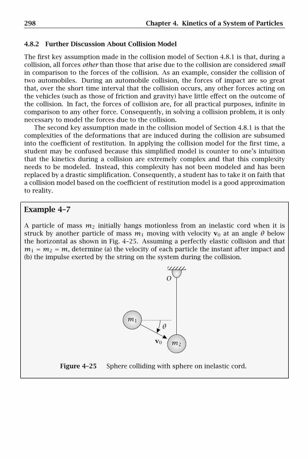
298 Chapter 4. Kinetics of a System of Particles
4.8.2 Further Discussion About Collision Model
The first key assumption made in the collision model of Section 4.8.1 is that, during acollision, all forces other than those that arise due to the collision are considered smallin comparison to the forces of the collision. As an example, consider the collision oftwo automobiles. During an automobile collision, the forces of impact are so greatthat, over the short time interval that the collision occurs, any other forces acting onthe vehicles (such as those of friction and gravity) have little effect on the outcome ofthe collision. In fact, the forces of collision are, for all practical purposes, infinite incomparison to any other force. Consequently, in solving a collision problem, it is onlynecessary to model the forces due to the collision.
The second key assumption made in the collision model of Section 4.8.1 is that thecomplexities of the deformations that are induced during the collision are subsumedinto the coefficient of restitution. In applying the collision model for the first time, astudent may be confused because this simplified model is counter to one’s intuitionthat the kinetics during a collision are extremely complex and that this complexityneeds to be modeled. Instead, this complexity has not been modeled and has beenreplaced by a drastic simplification. Consequently, a student has to take it on faith thata collision model based on the coefficient of restitution model is a good approximationto reality.
Example 4–7
A particle of mass m2 initially hangs motionless from an inelastic cord when it isstruck by another particle of mass m1 moving with velocity v0 at an angle θ belowthe horizontal as shown in Fig. 4–25. Assuming a perfectly elastic collision and thatm1 =m2 =m, determine (a) the velocity of each particle the instant after impact and(b) the impulse exerted by the string on the system during the collision.
v0
m1
m2
O
θ
Figure 4–25 Sphere colliding with sphere on inelastic cord.

4.8 Collision of Particles 299
Solution to Example 4–7
Kinematics
Let F be a fixed reference frame. Then choose the following coordinate system fixedin reference frame F :
Origin at OEx = Along Om2 at t = 0−
Ez = Out of pageEy = Ez × Ex
where t = 0− is the instant before impact. Because Ex,Ey,Ez is a fixed basis, thevelocity of each particle can be written as
Fv1 = v1xEx + v1yEy (4–434)Fv2 = v2xEx + v2yEy (4–435)
It is noted that, because we will be using the principle of linear impulse and linearmomentum to solve this problem, it is not necessary to compute the acceleration ofeach particle.
Kinetics
The next step is to apply linear impulse and linear momentum to the particles. Forthis problem, it is convenient to apply linear impulse and linear momentum to thefollowing two systems: (1) particle m1 and (2) particles m1 and m2. Each of thesekinetic analyses is now performed.
Application of Linear Impulse and Linear Momentum to Particle m1
Applying linear impulse and linear momentum to particle A, we have
F1 = FG′1 − FG1 (4–436)
Examining the free body diagram of particle m1 as shown in Fig. 4–26, it is seen thatthe only impulse acting on m1 during the collision is due to particle m2.
P
Figure 4–26 Free body diagram of particle m1 for Example 4–25.
We denote the impulse applied by m2 on m1 by P, and observe that P must lie alongthe line of v0, i.e.,
P = P sinθEx + P cosθEy (4–437)
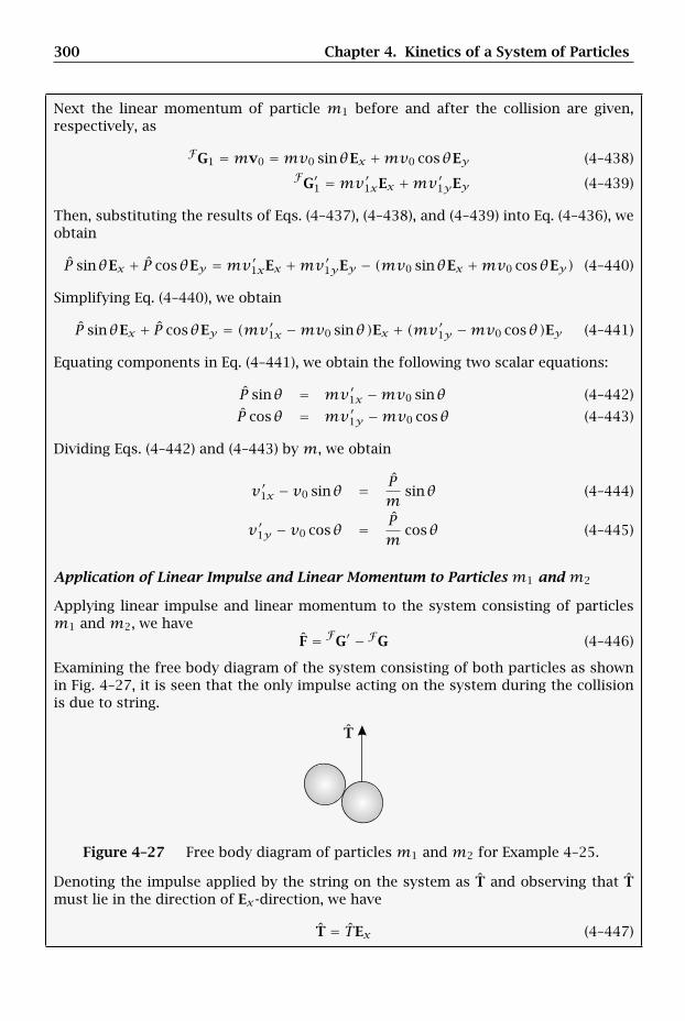
300 Chapter 4. Kinetics of a System of Particles
Next the linear momentum of particle m1 before and after the collision are given,respectively, as
FG1 =mv0 =mv0 sinθEx +mv0 cosθEy (4–438)FG′1 =mv′1xEx +mv′1yEy (4–439)
Then, substituting the results of Eqs. (4–437), (4–438), and (4–439) into Eq. (4–436), weobtain
P sinθEx + P cosθEy =mv′1xEx +mv′1yEy − (mv0 sinθEx +mv0 cosθEy) (4–440)
Simplifying Eq. (4–440), we obtain
P sinθEx + P cosθEy = (mv′1x −mv0 sinθ)Ex + (mv′1y −mv0 cosθ)Ey (4–441)
Equating components in Eq. (4–441), we obtain the following two scalar equations:
P sinθ = mv′1x −mv0 sinθ (4–442)
P cosθ = mv′1y −mv0 cosθ (4–443)
Dividing Eqs. (4–442) and (4–443) by m, we obtain
v′1x − v0 sinθ = Pm
sinθ (4–444)
v′1y − v0 cosθ = Pm
cosθ (4–445)
Application of Linear Impulse and Linear Momentum to Particles m1 and m2
Applying linear impulse and linear momentum to the system consisting of particlesm1 and m2, we have
F = FG′ − FG (4–446)
Examining the free body diagram of the system consisting of both particles as shownin Fig. 4–27, it is seen that the only impulse acting on the system during the collisionis due to string.
T
Figure 4–27 Free body diagram of particles m1 and m2 for Example 4–25.
Denoting the impulse applied by the string on the system as T and observing that Tmust lie in the direction of Ex-direction, we have
T = TEx (4–447)

4.8 Collision of Particles 301
Next, the linear momenta of the system before and after the collision are given, respec-tively, as
FG = mv0 =mv0 sinθEx +mv0 cosθEy (4–448)FG′ = mv′1xEx +mv′1yEy +mv′2xEx +mv′2yEy (4–449)
Substituting the results of Eqs. (4–447), (4–448), and (4–449) into Eq. (4–446), we obtain
TEx =mv′1xEx+mv′1yEy+mv′2xEx+mv′2yEy−(mv0 sinθEx+mv0 cosθEy) (4–450)
Simplifying Eq. (4–450), we have
TEx = (mv′1x +mv′2x −mv0 sinθ)Ex + (mv′1y +mv′2y −mv0 cosθ)Ey (4–451)
Equating components in Eq. (4–451), we obtain the following two scalar equations:
T = mv′1x +mv′2x −mv0 sinθ (4–452)
0 = mv′1y +mv′2y −mv0 cosθ (4–453)
Dividing Eqs. (4–452) and (4–453) by m, we obtain
v′1x + v′2x − v0 sinθ = Tm
(4–454)
v′1y + v′2y − v0 cosθ = 0 (4–455)
Kinematic Constraints During Impact
It can be seen that Eqs. (4–444), (4–445), (4–454), and (4–455) are a system of fourequations in the six unknowns v′1x , v′1y , v′2x , v′2y , P , and T . Consequently, two moreindependent equations are required in order to determine the solution. These twoequations are obtained from the kinematic constraints that act on the particles duringimpact. First, because the cord is inelastic, the component of velocity of mass m2 theinstant after impact must be zero, i.e.,
v′2x = 0 (4–456)
Second, because the collision is perfectly elastic, the coefficient of restitution, e, be-tween the two particles must be unity, i.e., e = 1. Applying the coefficient of restitutioncondition of Eq. (4–404) on page 294, we have
e =Fv′2 · n− Fv′1 · nFv1 · n− Fv2 · n
= 1 (4–457)
where n is the direction of impact. Now, because in this problem the impact occurs inthe direction of v0, we have
n = v0
‖v0‖= v0 sinθEx + v0 cosθEy
v0= sinθEx + cosθEy (4–458)
Substituting the expression for n from Eq. (4–458) into Eq. (4–457) along with the ex-pressions for the pre-impact and post-impact velocities of the particles, we obtain
v′2x sinθ + v′2y cosθ − (v′1x sinθ + v′1y cosθ)v0
= 1 (4–459)
302 Chapter 4. Kinetics of a System of Particles
Rearranging Eq. (4–459) gives
v′2x sinθ + v′2y cosθ − v′1x sinθ − v′1y cosθ − v0 = 0 (4–460)
Determination of Post-Impact Velocities and Impulse Exerted by Cord
The post-impact velocity of each particle and the impulse exerted by the cord on thesystem can now be determined using the results of Eqs. (4–444), (4–445), (4–454),(4–455), (4–456), and (4–460). First, multiplying Eq. (4–444) by sinθ and multiplyingEq. (4–445) by cosθ , we obtain
Pm
sin2θ = v′1x sinθ − v0 sin2θ (4–461)
Pm
cos2θ = v′1y cosθ − v0 cos2θ (4–462)
Adding Eqs. (4–461) and (4–462), we obtain
Pm= v′1x sinθ + v′1y cosθ − v0 (4–463)
Rearranging Eq. (4–463), we obtain
v′1x sinθ + v′1y cosθ = Pm+ v0 (4–464)
Then, substituting the result of Eq. (4–456) into (4–460), we have
v′2y cosθ − v′1x sinθ − v′1y cosθ − v0 = 0 (4–465)
Next, substituting the result of Eq. (4–464) into (4–465), we obtain
v′2y cosθ −(Pm+ v0
)− v0 = 0 (4–466)
Simplifying Eq. (4–466), we obtain
v′2y cosθ = Pm+ 2v0 (4–467)
Then, multiplying Eq. (4–455) by cosθ and solving for v′2y cosθ gives
v′2y cosθ = −v′1y cosθ + v0 cos2θ (4–468)
Furthermore, solving Eq. (4–455) for v′1y cosθ gives
v′1y cosθ = Pm
cos2θ + v0 cos2θ (4–469)
Substituting the result of Eq. (4–469) into (4–468) gives
v′2y cosθ = −(Pm
cos2θ + v0 cos2θ)+ v0 cos2θ = − P
mcos2θ (4–470)
4.8 Collision of Particles 303
Then, setting the results of Eqs. (4–467) and (4–470) equal, we have
Pm+ 2v0 = − Pm cos2θ (4–471)
Solving Eq. (4–471) for P gives
P = − 2mv0
1+ cos2θ(4–472)
Then, substituting the result of Eq. (4–472) into (4–444) gives
− 2v0
1+ cos2θsinθ = v′1x − v0 sinθ (4–473)
Solving Eq. (4–473) for v′1x gives
v′1x = −2v0
1+ cos2θsinθ + v0 sinθ = v0
(1− 2
1+ cos2θ
)sinθ (4–474)
Simplifying Eq. (4–474), we obtain v′1x as
v′1x = −v0sin2θ
1+ cos2θsinθ (4–475)
Similarly, substituting the result of Eq. (4–472) into (4–445) gives
− 2v0 cosθ1+ cos2θ
= v′1y − v0 cosθ (4–476)
Solving Eq. (4–476) for v′1y gives
v′1y = v0
(1− 2
1+ cos2θ
)cosθ = −v0
sin2θ1+ cos2θ
cosθ (4–477)
Then, substituting the result of Eqs. (4–477) into (4–455), we obtain
v0
(1− 2
1+ cos2θ
)cosθ + v′2y − v0 cosθ = 0 (4–478)
Solving Eq. (4–478) for v′2y , we obtain
v′2y = v0 cosθ − v0
(1− 2
1+ cos2θ
)cosθ = 2v0 cosθ
1+ cos2θ(4–479)
Substituting the results of Eqs. (4–474) and (4–456) into Eq. (4–454), we have
Tm= v0
(1− 2
1+ cos2θ
)sinθ − v0 sinθ = − 2v0 sinθ
1+ cos2θ(4–480)
Solving Eq. (4–480) for T , we obtain
T = −2mv0 sinθ1+ cos2θ
(4–481)
304 Chapter 4. Kinetics of a System of Particles
Then, substituting the result of Eq. (4–481) into (4–447), the impulse exerted by thecord on the system during the impact is given as
T = −2mv0 sinθ1+ cos2θ
Ex (4–482)
Finally, using the results of Eqs. (4–475), (4–477), and (4–479), the post-impact veloci-ties of particles m1 and m2 are given, respectively, as
Fv′1 = −v0sin2θ
1+ cos2θsinθEx +−v0
sin2θ1+ cos2θ
cosθEy (4–483)
Fv′2 = 2v0 cosθ1+ cos2θ
Ey (4–484)
Summary of Chapter 4 305
Summary of Chapter 4
This chapter was devoted to developing the framework for solving and analyzing prob-lems involving a system of particles. The first topics covered in this Chapter were thecenter of mass, linear momentum, and angular momentum of a rigid body. The posi-tion of the center of mass for a system of particles was defined as
r =∑ni=1miri∑ni=1mi
=∑ni=1mirim
(4–1)
where ri (i = 1, . . . , n) is the position of particle i measured relative to a point O fixedin an inertial reference frame N . The linear momentum for a system of particles wasthen defined as
NG =n∑i=1
miNvi (4–3)
where Nvi (i = 1, . . . , n) is the velocity of particle i in the inertial reference frame N .It was then shown that the linear momentum for a system of particles can be writtenas
NG =Nddt(mr) =m
Ndrdt
=mNv (4–8)
where Nv is the velocity of the center of mass of the system in the inertial referenceframe N . It was then shown that the velocity of the center of mass in reference frameN can be written as
Nv =∑ni=1mi
Nvim
(4–9)
Finally, the acceleration of the center of mass of the system in the inertial referenceframe N was defined as
Na =∑ni=1mi
Naim
(4–11)
The next topic covered in this chapter was the angular momentum for a system ofparticles. First, the angular momentum of a system of particles in an inertial referenceframe N relative to an arbitrary reference point Q was defined as
NHQ =n∑i=1
(ri − rQ)×mi(Nvi −NvQ) (4–15)
Furthermore, the angular momentum relative to a pointO fixed in the inertial referenceframe N , denoted NHO , was defined as
NHO =n∑i=1
(ri − rO)×miNvi (4–16)
Finally, the angular momentum relative to the center of mass of the system, denotedN
H, was defined asN
H =n∑i=1
(ri − r)×mi(Nvi −Nv) (4–17)
306 Chapter 4. Kinetics of a System of Particles
Using the three definitions of angular momentum, it was shown that NHQ and NHOare related as
NHQ = NHO − (r− rQ)×mNvQ − (rQ − rO)×mNv (4–23)
Next, it was shown thatN
H and NHO are related as
NH = NHO − (r− rO)×mNv (4–25)
Finally, it was shown that NHQ andN
H are related as
NHQ = NH+ (r− rQ)×m(Nv−NvQ) (4–28)
The next topic covered in this chapter was Newton’s 2nd law for a system of parti-cles. In particular, it was shown that
Ri =miNai (i = 1,2, . . . , n) (4–32)
where Nai is the acceleration of particle i in an inertial reference frame N and Ri isthe resultant force acting on particle i. Furthermore, it was shown that the resultantforce on particle i is given as
Ri = Fi +n∑j=1
fij (i = 1,2, . . . , n) (4–33)
where Fi is the resultant external force applied to particle i and∑nj=1 fij is the resultant
force on particle i applied by every other particle in the system. It was assumed thatthe forces of interaction between particles satisfy the strong form of Newton’s 3rd law,i.e., that fij = −fji and fij lies along the line between particle i and particle j. Usingthe properties of the forces of interaction, it was shown that the motion of the centerof mass of the system satisfies Newton’s 2nd law, i.e.,
F =mNa (4–38)
where F is the resultant external force applied to the system and Na is the accelerationof the center of mass of the system in an inertial reference frame N .
The next topic covered in this chapter was the moment applied by a system offorces to a system of particles. First, the moment due to a system of forces F1, . . . ,Fnrelative to an arbitrary reference point Q, denoted MQ, was defined as
MQ =n∑i=1
(ri − rQ)× Fi (4–75)
Next, the moment due to all external forces relative to a point O fixed in the inertialreference frame N , denoted MO , was defined as
MO =n∑i=1
(ri − rO)× Fi (4–76)
Finally, the moment due to all external forces relative to the center of mass of thesystem, denoted M, was defined as
M =n∑i=1
(ri − r)× Fi (4–77)
Summary of Chapter 4 307
The next topic covered in this chapter was the rate of change of angular momentumfor a system of particles. First, the rate of change of NHQ in the inertial referenceframe N was derived to be
MQ − (r− rQ)×mNaQ =Nddt
(NHQ
)(4–87)
where MQ is the moment due to all external forces relative to point Q as given inEq. (4–75). Furthermore, the quantity
−(r− rQ)×mNaQ (4–88)
was called the inertial moment of the reference point Q relative to the center of massof the system. Then, for the case of a reference point O fixed in an inertial referenceframe N , it was shown that
MO =Nddt
(NHO
)(4–89)
Similarly, for the case where the reference point is located at the center of mass of thesystem, it was shown that
M =Nddt
(NH)
(4–90)
Because Eqs. (4–89) and (4–90) have the same mathematical form, when the referencepoint is either fixed in an inertial reference frame or is the center of mass of the system,we have
M =Nddt
(NH
)(4–91)
Finally, it was emphasized that the relationship of Eq. (4–91) is not valid for any pointsother than a point fixed in an inertial reference frame or the center of mass. In thecase of an arbitrary reference point, it is necessary to use the result of Eq. (4–87).
The next topic covered in this chapter was impulse and momentum for a system ofparticles. First, the principle of linear impulse and linear momentum for a system ofparticles was derived as
F = NG(t2)−NG(t1) (4–216)
Next, the principle of angular impulse and angular momentum relative to an arbitraryreference point Q was derived as
MQ −∫ t2t1(r− rQ)×mNaQdt = NHQ(t2)−NHQ(t1) (4–221)
Then, for the case of a reference point O fixed in an inertial reference frame N , it wasshown that
MO = NHO(t2)−NHO(t1) (4–223)
Finally, for the case where the reference point is the center of mass of the system, itwas shown that
ˆM = NH(t2)−N
H(t1) (4–224)
The next topics covered in this chapter were work and energy for a system of par-ticles. First, kinetic energy for a system of particles in an inertial reference frame Nwas defined as
NT = 12
n∑i=1
miNvi · Nvi (4–307)
308 Chapter 4. Kinetics of a System of Particles
An alternate expression for the kinetic energy for a system of particles was also ob-tained as
NT = 12mNv · Nv+ 1
2
n∑i=1
mi
(Nvi −Nv
)·(Nvi −Nv
)(4–314)
The kinetic energy was then written in the more compact form
NT = NT(1) +NT(2) (4–315)
whereNT(1) = 1
2mNv · Nv (4–316)
NT(2) = 12
n∑i=1
mi
(Nvi −Nv
)·(Nvi −Nv
)(4–317)
Using Eq. (4–316), it was shown that
ddt
(NT(1)
)= F · Nv = NP(1) (4–320)
which states that the power of all external forces acting on a system of particles isequal to the rate of change of the kinetic energy due to the motion of the center ofmass of the system. Integrating Eq. (4–320) from time t = t1 to t = t2, it was shownthat
NT(1)(t2)−NT(1)(t1) = NW(1)12 (4–322)
Next, it was shown that the rate of change of the kinetic energy of a system of particlessatisfies
ddt
(NT
)=
n∑i=1
Ri · Nvi (4–330)
which is the work-energy theorem for a system of particles and states that the rate ofchange of kinetic energy of a system of particles is equal to the power produced by allinternal and external forces acting on the system. Finally, it was shown that
ddt
(NE
)=
n∑i=1
Rnci · Nvi (4–341)
which is the alternate form of the work-energy theorem for a system of particles andstates that the rate of change of total energy of a system of particles is equal to thepower produced by all of the nonconservative forces acting on the system.
The last topic covered in this Chapter was the collision of two particles. In partic-ular, a simplified collision model was derived that used an ad hoc parameter calledthe coefficient of restitution, e. In terms of e, it was shown that the pre-collision andpost-collision velocities of two particles undergoing an impact are related as
e =Nv′2 · n−Nv′1 · nNv1 · n−Nv2 · n
(4–404)
where n is the direction of the impact (also called the line of impact) and the notation(·)′ denotes a post-collision quantity. Furthermore, it was shown that the post-collision
Summary of Chapter 4 309
velocities of the particles are given as
Nv′1 = (Nv1 · u)
u+ (Nv1 ·w)
w
+(m1 − em2
m1 +m2
Nv1 · n+ m2(1+ e)m1 +m2
Nv2 · n)
n
Nv′2 = (Nv2 · u)
u+ (Nv2 ·w)
w
+(m1(1+ e)m1 +m2
Nv1 · n+ m2 − em1
m1 +m2
Nv2 · n)
n
(4–433)
where u and w lie in the plane tangent to the surface of each particle at the point ofcontact during the collision. Finally, it was discussed that the collision model is highlysimplified in that all of the kinetics associated with the impact are lumped into thecoefficient of restitution.

310 Chapter 4. Kinetics of a System of Particles
Problems for Chapter 4
4.1 A particle of mass m is connected to a block of mass M via a rigid massless rodof length l as shown in Fig. P4-1. The rod is free to pivot about a hinge attached tothe block at point O. Furthermore, the block rolls without friction along a horizontalsurface. Knowing that a horizontal force F is applied to the block and that gravity actsdownward, determine a system of two differential equations describing the motion ofthe block and the particle.
F
g
l
m
x
M
O
P
θ
Figure P4-1
4.2 A block of mass M is initially at rest atop a horizontal surface when it is struckby a ball bearing of mass m as shown in Fig. P4-2. The velocity of the particle asit strikes the block is v0 at an angle θ below the horizontal. Assuming a perfectlyinelastic impact, that the block is constrained to remain on the horizontal surface,and no gravity, determine the velocity of the block and the particle immediately afterimpact.
v0
m
M
θ
Figure P4-2
4.3 A block of massm is dropped from a height h above a plate of mass M as shownin Fig. P4-3. The plate is supported by three linear springs, each with spring constant K,and is initially in static equilibrium. Assuming that the compression of the springs dueto the weight of the plate is negligible, that the impact is perfectly inelastic, that theblock strikes the vertical center of the plate, and that gravity acts downward, determine(a) the velocity of the block and plate immediately after impact and (b) the maximumcompression, xmax, attained by the springs after impact.
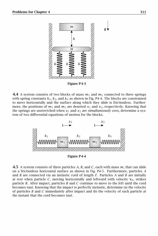
Problems for Chapter 4 311
gm
h
KKK
M
Figure P4-3
4.4 A system consists of two blocks of mass m1 and m2 connected to three springswith spring constants k1, k2, and k3 as shown in Fig. P4-4. The blocks are constrainedto move horizontally and the surface along which they slide is frictionless. Further-more, the positions of m1 and m2 are denoted x1 and x2, respectively. Knowing thatthe springs are unstretched when x1 and x2 are simultaneously zero, determine a sys-tem of two differential equations of motion for the blocks.
k1 k2 k3
m1 m2
x1 x2
Figure P4-4
4.5 A system consists of three particles A, B, and C , each with massm, that can slideon a frictionless horizontal surface as shown in Fig. P4-5. Furthermore, particles Aand B are connected via an inelastic cord of length . Particles A and B are initiallyat rest when particle C , moving horizontally and leftward with velocity v0, strikesparticle B. After impact, particles B and C continue to move to the left until the cordbecomes taut. Knowing that the impact is perfectly inelastic, determine (a) the velocityof particles B and C immediately after impact and (b) the velocity of each particle atthe instant that the cord becomes taut.
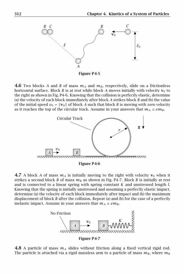
312 Chapter 4. Kinetics of a System of Particles
0
v0
A
B BC C
Figure P4-5
4.6 Two blocks A and B of mass mA and mB , respectively, slide on a frictionlesshorizontal surface. Block B is at rest while block A moves initially with velocity v0 tothe right as shown in Fig. P4-6. Knowing that the collision is perfectly elastic, determine(a) the velocity of each block immediately after block A strikes block B and (b) the valueof the initial speed v0 = ‖v0‖ of block A such that block B is moving with zero velocityas it reaches the top of the circular track. Assume in your answers that mA ≤ emB .
Circular Track
gr
v0A B
Figure P4-6
4.7 A block A of mass mA is initially moving to the right with velocity v0 when itstrikes a second block B of mass mB as shown in Fig. P4-7. Block B is initially at restand is connected to a linear spring with spring constant K and unstressed length l.Knowing that the spring is initially unstressed and assuming a perfectly elastic impact,determine (a) the velocity of each block immediately after impact and (b) the maximumdisplacement of block B after the collision. Repeat (a) and (b) for the case of a perfectlyinelastic impact. Assume in your answers that mA ≤ emB .
No Friction
v0A B
K
Figure P4-7
4.8 A particle of mass mA slides without friction along a fixed vertical rigid rod.The particle is attached via a rigid massless arm to a particle of mass mB , where mB

Problems for Chapter 4 313
slides without friction along a fixed horizontal rigid rod. Assuming that θ is the anglebetween the horizontal rod and the arm and that gravity acts downward, determinethe differential equation of motion for the system in terms of the angle θ.
g
l
mA
mB
A
BOθ
Figure P4-8
4.9 Two particles of mass M and m, with positions r1 and r2, respectively, move inthree dimensions as shown in Fig. P4-9. Knowing that the only force acting on eachparticle is due to the gravitational attraction of the other body and that the gravita-tional attraction obeys the universal law of gravitation, determine (a) the differentialequation describing the motion of mass m, (b) the differential equation describing themotion of mass M , and (c) the differential equation describing the motion of mass mrelative to mass M .
Assume now that m << M and µ = GM . Using this approximation and the resultof part (c) determine (d) the differential equation of mass m relative to mass M . Inaddition, show that (e) the energy of the system in (d) is conserved and that (f) theangular momentum of the system in (d) relative to M is conserved.
r
r1 r2
m
x
y
z
M
O
Figure P4-9
4.10 A particle of mass m2 is suspended from a rigid massless rod as shown inFig. P4-10. The rod is attached at its other end to a collar of mass m1. The collar,in turn, slides without friction along a horizontal track. Furthermore, the collar is at-tached to a linear spring with spring constant K and unstretched length 0. Assumingthat gravity acts downward, determine a system of two differential equations in termsof the variables x and θ that describes the motion of the collar and the particle.

314 Chapter 4. Kinetics of a System of Particles
gl
m1
m2
x
O
P
θ
Figure P4-10
4.11 Particle A of mass m/2 is moving with an initial velocity v0 to the right when itstrikes particle B, also of massm/2, as shown in Fig. P4-11. Particle B is connected viaa rigid massless rod to a cart C of massm. The cart rolls without friction along a fixedhorizontal surface. Knowing that the collision is perfectly inelastic, determine (a) thevelocity of each particle and the velocity of the cart immediately after impact and (b)the maximum angle θ attained by the rod after the collision.
No Frictiong
v0A B
CO
Figure P4-11
4.12 A dumbbell of mass 2m and length 2a is welded to a rigid massless rod of lengthl to form the shape of the letter “T”. The T-shaped dumbbell is hinged at the free endof the height of the “T” to the fixed point O as shown in Fig. P4-12. Knowing that θis the angle formed by the height of the “T” with the vertically downward directionand that gravity acts downward, determine the differential equation of motion of thedumbbell in terms of the angle θ using (a) a balance of angular momentum (b) one ofthe forms of the work-energy theorem.

Problems for Chapter 4 315
g
l
2a
m
m
O
Pθ
Figure P4-12
4.13 A system consists of two small blocks of mass m1 and m2. The blocks slidewithout friction inside a circular slot of radius R cut from a disk of radius R as shownin Fig. P4-13. Furthermore, a linear spring with spring constant K and unstretchedlength 0 is attached between the two blocks. Knowing that the angle θ1 describes theposition of m1 while the angle θ2 describes the position m2, that the spring cannotbend, and that gravity acts downward, determine a system of two differential equationsof motion for the blocks.
g
m1
m2
K
O R
θ1
θ2
Figure P4-13
4.14 A system consists of two blocks A and B of masses mA and mB , respectively,that slide along a frictionless surface as shown in Fig. P4-14. The blocks are connectedby a linear spring with spring constant K and unstretched length . Assuming that theblocks are initially at rest and the spring is initially unstretched when block A is struckby a horizontal impulse P, determine the velocity of each block immediately after theapplication of the impulse.
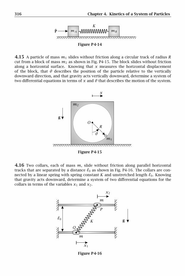
316 Chapter 4. Kinetics of a System of Particles
P mA mB
K
Figure P4-14
4.15 A particle of mass m1 slides without friction along a circular track of radius Rcut from a block of mass m2 as shown in Fig. P4-15. The block slides without frictionalong a horizontal surface. Knowing that x measures the horizontal displacementof the block, that θ describes the position of the particle relative to the verticallydownward direction, and that gravity acts vertically downward, determine a system oftwo differential equations in terms of x and θ that describes the motion of the system.
g
m1
m2
x
OR
θ
Figure P4-15
4.16 Two collars, each of mass m, slide without friction along parallel horizontaltracks that are separated by a distance 0 as shown in Fig. P4-16. The collars are con-nected by a linear spring with spring constant K and unstretched length 0. Knowingthat gravity acts downward, determine a system of two differential equations for thecollars in terms of the variables x1 and x2.
0 g
m
m
x1
x2
K
P
Q
Figure P4-16
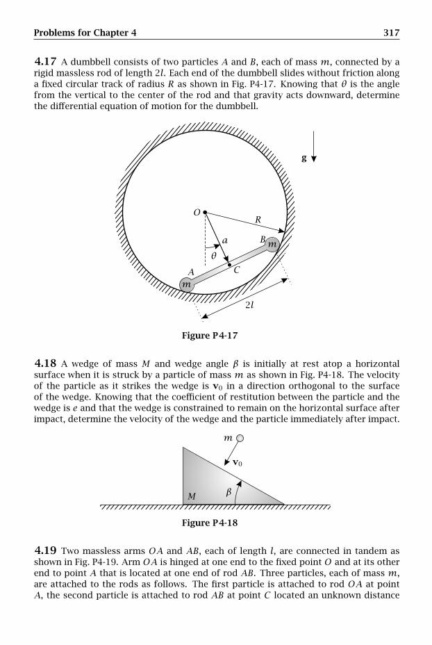
Problems for Chapter 4 317
4.17 A dumbbell consists of two particles A and B, each of mass m, connected by arigid massless rod of length 2l. Each end of the dumbbell slides without friction alonga fixed circular track of radius R as shown in Fig. P4-17. Knowing that θ is the anglefrom the vertical to the center of the rod and that gravity acts downward, determinethe differential equation of motion for the dumbbell.
2l
g
a m
mA
B
C
OR
θ
Figure P4-17
4.18 A wedge of mass M and wedge angle β is initially at rest atop a horizontalsurface when it is struck by a particle of mass m as shown in Fig. P4-18. The velocityof the particle as it strikes the wedge is v0 in a direction orthogonal to the surfaceof the wedge. Knowing that the coefficient of restitution between the particle and thewedge is e and that the wedge is constrained to remain on the horizontal surface afterimpact, determine the velocity of the wedge and the particle immediately after impact.
v0
m
M β
Figure P4-18
4.19 Two massless arms OA and AB, each of length l, are connected in tandem asshown in Fig. P4-19. Arm OA is hinged at one end to the fixed point O and at its otherend to point A that is located at one end of rod AB. Three particles, each of mass m,are attached to the rods as follows. The first particle is attached to rod OA at pointA, the second particle is attached to rod AB at point C located an unknown distance
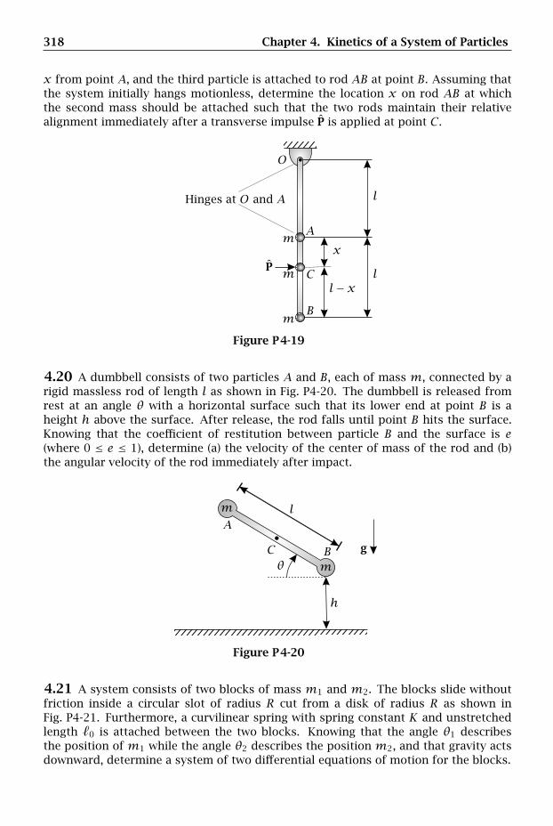
318 Chapter 4. Kinetics of a System of Particles
x from point A, and the third particle is attached to rod AB at point B. Assuming thatthe system initially hangs motionless, determine the location x on rod AB at whichthe second mass should be attached such that the two rods maintain their relativealignment immediately after a transverse impulse P is applied at point C .
Hinges at O and A
P l
l
m
m
m
l− x
x
A
B
C
O
Figure P4-19
4.20 A dumbbell consists of two particles A and B, each of mass m, connected by arigid massless rod of length l as shown in Fig. P4-20. The dumbbell is released fromrest at an angle θ with a horizontal surface such that its lower end at point B is aheight h above the surface. After release, the rod falls until point B hits the surface.Knowing that the coefficient of restitution between particle B and the surface is e(where 0 ≤ e ≤ 1), determine (a) the velocity of the center of mass of the rod and (b)the angular velocity of the rod immediately after impact.
g
l
m
m
h
A
BCθ
Figure P4-20
4.21 A system consists of two blocks of mass m1 and m2. The blocks slide withoutfriction inside a circular slot of radius R cut from a disk of radius R as shown inFig. P4-21. Furthermore, a curvilinear spring with spring constant K and unstretchedlength 0 is attached between the two blocks. Knowing that the angle θ1 describesthe position of m1 while the angle θ2 describes the position m2, and that gravity actsdownward, determine a system of two differential equations of motion for the blocks.
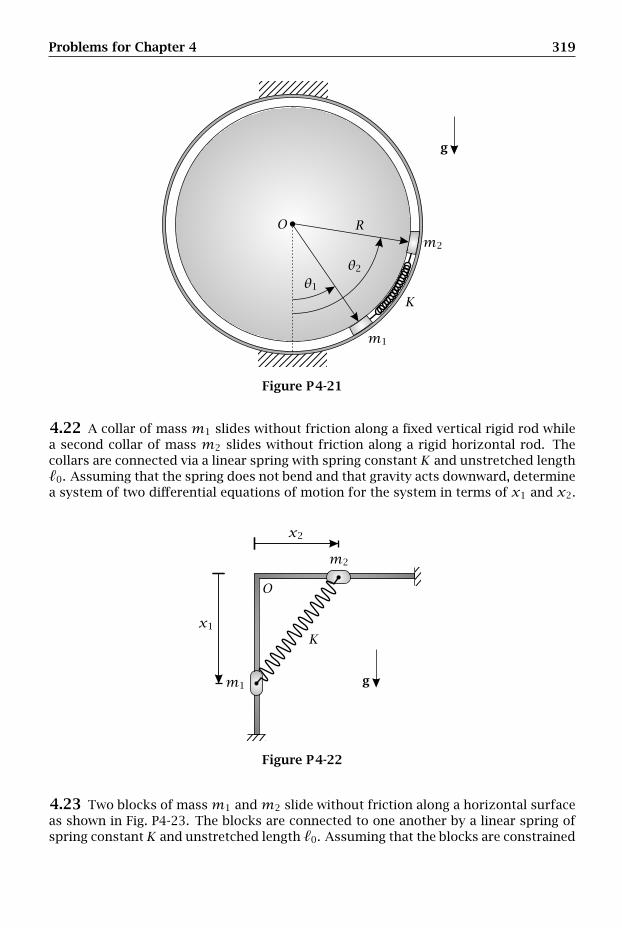
Problems for Chapter 4 319
g
m1
m2
K
O R
θ1
θ2
Figure P4-21
4.22 A collar of mass m1 slides without friction along a fixed vertical rigid rod whilea second collar of mass m2 slides without friction along a rigid horizontal rod. Thecollars are connected via a linear spring with spring constant K and unstretched length0. Assuming that the spring does not bend and that gravity acts downward, determinea system of two differential equations of motion for the system in terms of x1 and x2.
gm1
m2
x1
x2
K
O
Figure P4-22
4.23 Two blocks of massm1 andm2 slide without friction along a horizontal surfaceas shown in Fig. P4-23. The blocks are connected to one another by a linear spring ofspring constant K and unstretched length 0. Assuming that the blocks are constrained
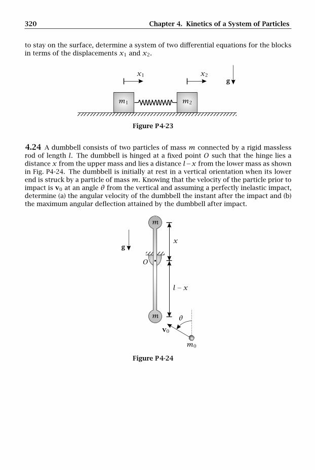
320 Chapter 4. Kinetics of a System of Particles
to stay on the surface, determine a system of two differential equations for the blocksin terms of the displacements x1 and x2.
g
m1 m2
x1 x2
Figure P4-23
4.24 A dumbbell consists of two particles of mass m connected by a rigid masslessrod of length l. The dumbbell is hinged at a fixed point O such that the hinge lies adistance x from the upper mass and lies a distance l−x from the lower mass as shownin Fig. P4-24. The dumbbell is initially at rest in a vertical orientation when its lowerend is struck by a particle of massm. Knowing that the velocity of the particle prior toimpact is v0 at an angle θ from the vertical and assuming a perfectly inelastic impact,determine (a) the angular velocity of the dumbbell the instant after the impact and (b)the maximum angular deflection attained by the dumbbell after impact.
g
v0
m
m
m0
l− x
x
O
θ
Figure P4-24
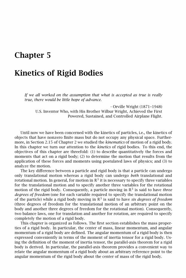
Chapter 5
Kinetics of Rigid Bodies
If we all worked on the assumption that what is accepted as true is reallytrue, there would be little hope of advance.
- Orville Wright (1871–1948)U.S. Inventor Who, with His Brother Wilbur Wright, Achieved the First
Powered, Sustained, and Controlled Airplane Flight.
Until now we have been concerned with the kinetics of particles, i.e., the kinetics ofobjects that have nonzero finite mass but do not occupy any physical space. Further-more, in Section 2.15 of Chapter 2 we studied the kinematics of motion of a rigid body.In this chapter we turn our attention to the kinetics of rigid bodies. To this end, theobjectives of this chapter are threefold: (1) to describe quantitatively the forces andmoments that act on a rigid body; (2) to determine the motion that results from theapplication of these forces and moments using postulated laws of physics; and (3) toanalyze the motion.
The key difference between a particle and rigid body is that a particle can undergoonly translational motion whereas a rigid body can undergo both translational androtational motion. In general, for motion in R3 it is necessary to specify three variablesfor the translational motion and to specify another three variables for the rotationalmotion of the rigid body. Consequently, a particle moving in R3 is said to have threedegrees of freedom (one for each variable required to specify the translational motionof the particle) while a rigid body moving in R3 is said to have six degrees of freedom(three degrees of freedom for the translational motion of an arbitrary point on thebody and another three degrees of freedom for the rotational motion). Consequently,two balance laws, one for translation and another for rotation, are required to specifycompletely the motion of a rigid body.
This chapter is organized as follows. The first section establishes the mass proper-ties of a rigid body. In particular, the center of mass, linear momentum, and angularmomentum of a rigid body are defined. The angular momentum of a rigid body is thenexpressed conveniently in terms of the moment of inertia tensor for a rigid body. Us-ing the definition of the moment of inertia tensor, the parallel-axis theorem for a rigidbody is derived. In particular, the parallel-axis theorem provides a convenient way torelate the angular momentum of a rigid body about an arbitrary reference point to theangular momentum of the rigid body about the center of mass of the rigid body.
322 Chapter 5. Kinetics of Rigid Bodies
Using the mass properties given in the first section, the second section establishesthe laws of kinetics of a rigid body. First, the two different types of allowable actionsthat can be applied to a rigid body, namely forces and pure torques, are described.Then, using the definitions of linear momentum and angular momentum of a rigidbody, the fundamental postulates for the kinetics of a rigid body, called Euler’s laws,are stated. Using the postulated laws of kinetics of a rigid body, two alternate formsof Euler’s 2nd law are derived. Next, the kinetic energy of a rigid body is definedfrom which the work-energy theorem for a rigid body is derived. Finally, using Euler’s1st law and three forms of Euler’s 2nd law, the concepts of linear impulse and linearmomentum and angular impulse and angular momentum for a rigid body are derived.Similar to the approach used in previous chapters, the understanding of rigid bodykinetics is facilitated through the systematic application of the concepts to exampleproblems.
5.1 Center of Mass and Linear Momentum of a Rigid Body
5.1.1 Center of Mass of a Rigid Body
Let R be a rigid body (as defined in Chapter 2) and let r be the position of a point P onR. Finally, let N be an inertial reference frame. Then the center of mass of the rigidbody R is defined as
r =
∫R
rdm∫Rdm
(5–1)
where the notation ∫Rdm (5–2)
means that the integral is being taken over all points in R3 occupied by R and dm is adifferential mass element. Denoting the volume of the rigid body by V , the differentialmass element dm is given as
dm = ρdV (5–3)
where ρ is mass density per unit volume of R and dV is a differential volume element.Consequently, it is seen that the integral of Eq. (5–2) represents a volume integral overall points on R.1 Furthermore, it is seen that the mass of the rigid body is given as
m =∫Rdm =
∫RρdV (5–4)
Now because a rigid body cannot change in mass, we note that m is a constant. Thecenter of mass of a rigid body can then be written as
r =
∫R
rdm
m(5–5)
1From this point forth the notation of Eq. (5–2) will always be used to denote a volume integral.
5.2 Angular Momentum of a Rigid Body 323
5.1.2 Linear Momentum of a Rigid Body
Let Nv = Ndr/dt be the velocity of a point P on a rigid body R as viewed by an ob-server in an inertial reference frame N . Then the linear momentum of R in referenceframe N is defined as
NG =∫RNvdm (5–6)
Equation (5–6) can also be written as
NG =∫R
Ndrdtdm (5–7)
Because the integral is being computed over the body, the rate of change is indepen-dent of the integral. Therefore, the order of integration and differentiation in Eq. (5–7)can be interchanged to give
NG =Nddt
∫R
rdm (5–8)
Substituting Eq. (5–5) into (5–8), we obtain
NG =Nddt(mr) =m
Ndrdt
=mNv (5–9)
The quantity Nv = Ndr/dt is the velocity of the center of mass of the rigid body inreference frame N . It is noted that Nv can also be written as
Nv =
∫RNvdm
m(5–10)
Finally, the acceleration of the center of mass of a rigid body as viewed by an observerin an inertial reference frame N , denoted Na, is defined as
Na =
∫RNadm
m(5–11)
It is noted that the acceleration of the center of mass is also given as
Na =Nddt
(Nv
)(5–12)
5.2 Angular Momentum of a Rigid Body
The angular momentum of a rigid body R relative to an arbitrary reference point Q inan inertial reference frame N is defined as2
NHQ =∫R(r− rQ)× (Nv−NvQ)dm (5–13)
2It is noted again that the angular momentum is defined using the relative velocity Nv − NvQ and isconsistent with the definition used in Greenwood (1977; 1988).
324 Chapter 5. Kinetics of Rigid Bodies
where rQ and NvQ are the position and velocity of point Q, respectively. The angularmomentum of a rigid body relative to a point O fixed in an inertial reference frame Nis defined as
NHO =∫R(r− rO)×Nvdm (5–14)
The angular momentum of a rigid body relative to the center of mass of the rigid bodyin an inertial reference frame N is defined as
NH =
∫R(r− r)× (Nv−Nv)dm (5–15)
We can obtain a relationship between NHQ and NHO by subtracting Eq. (5–14) from(5–13). This gives
NHQ −NHO =∫R(r− rQ)× (Nv−NvQ)dm−
∫R(r− rO)×Nvdm (5–16)
Expanding Eq. (5–16), we have
NHQ −NHO =∫R
(r×Nv− r×NvQ − rQ ×Nv+ rQ ×NvQ
)dm
+∫R
(−r×Nv+ rO ×Nv
)dm
(5–17)
Observing that the first and fifth terms in the integral cancel, Eq. (5–17) simplifies to
NHQ −NHO =∫R
(−r×NvQ − rQ ×Nv+ rQ ×NvQ + rO ×Nv
)dm (5–18)
Now, because rO , rQ and NvQ are independent of the integral, we have∫R
r×NvQdm = r×mNvQ∫R
rQ ×Nvdm = rQ ×mNv∫R
rQ ×NvQdm = rQ ×mNvQ∫R
rO ×Nvdm = rO ×mNv
(5–19)
Equation (5–18) can then be written as
NHQ −NHO = −r×mNvQ − rQ ×mNv+ rQ ×mNvQ + rO ×mNv (5–20)
Equation (5–20) simplifies to
NHQ = NHO − (r− rQ)×mNvQ − (rQ − rO)×mNv (5–21)
Next, using the result of Eq. (5–21), a relationship between NHO andN
H is obtained bysetting the reference point in Eq. (5–21) equal to the center of mass of the rigid bodyas
NH = NHO − (r− rO)×mNv (5–22)
5.3 Moment of Inertia Tensor of a Rigid Body 325
Finally, by substituting the result of Eq. (5–22) into (5–21), we can obtain a relationshipbetween NHQ and
NH as
NHQ = NH+ (r− rO)×mNv− (r− rQ)×mNvQ − (rQ − rO)×mNv (5–23)
Equation (5–23) then simplifies to
NHQ = NH+ (rQ − r)×m(NvQ −Nv) (5–24)
5.3 Moment of Inertia Tensor of a Rigid Body
Quite often in rigid body dynamics it is useful to compute the angular momentumrelative to a point that is fixed in the rigid body. In such cases an elegant expressionfor the angular momentum of the rigid body can be derived in terms of the momentof inertia tensor. In this section we derive the moment of inertia tensor of a rigid bodyand describe how to compute the angular momentum of the rigid body in terms of themoment of inertia tensor.
5.3.1 Moment of Inertia Tensor Relative to a Body-Fixed Point
Let P be a point fixed in a rigid body R and let Nv be the velocity of P in an inertialreference frame N . Furthermore, let Q be an arbitrary point fixed in R and let NvQbe the velocity of point Q in the inertial reference frame N . Finally, let NωR be theangular velocity of R in the inertial reference frame. Then, because P and Q are bothpoints that are fixed in R, the velocity P relative to Q in reference frame N is givenfrom Eq. (2–516) on page 106 as
Nv−NvQ = NωR × (r− rQ) (5–25)
Substituting Eq. (5–25) into the expression for NHQ from Eq. (5–13), we obtain
NHQ =∫R(r− rQ)×
[NωR × (r− rQ)
]dm (5–26)
Now suppose that we letρQ = r− rQ (5–27)
Equation (5–26) can then be written in terms of ρQ as
NHQ =∫RρQ ×
(NωR × ρQ
)dm (5–28)
Then, using the vector triple product as given in Eq. (1–29) on page 10, we have
ρQ ×(NωR × ρQ
)=(ρQ · ρQ
)NωR −
(ρQ · NωR
)ρQ (5–29)
Using the result of Eq. (5–29), Eq. (5–28) becomes
NHQ =∫R
[(ρQ · ρQ
)NωR −
(ρQ · NωR
)ρQ
]dm (5–30)

326 Chapter 5. Kinetics of Rigid Bodies
Using the definition of the product between a tensor and a vector from Eq. (1–41) onpage 11, the second term in the integrand of Eq. (5–30) can be written as(
ρQ · NωR)ρQ = ρQ
(ρQ · NωR
)=(ρQ ⊗ ρQ
)· NωR (5–31)
Substituting the result of Eq. (5–31) into (5–30), we obtain
NHQ =∫R
[(ρQ · ρQ
)NωR −
(ρQ ⊗ ρQ
)· NωR
]dm (5–32)
Furthermore, recalling the identity tensor U from Eq. (1–34), we have
NωR = U · NωR (5–33)
Substituting the result of Eq. (5–33), we obtain
NHQ =∫R
[(ρQ · ρQ
)U · NωR −
(ρQ ⊗ ρQ
)· NωR
]dm (5–34)
Now we note that NωR is a property of the rigid body and, hence, is independent ofthe integral. Therefore, Eq. (5–34) can be written as
NHQ =∫
R
[(ρQ · ρQ
)U−
(ρQ ⊗ ρQ
)]dm
· NωR (5–35)
The quantity
IRQ =∫R
[(ρQ · ρQ
)U−
(ρQ ⊗ ρQ
)]dm (5–36)
is called the moment of inertia tensor of the rigid bodyR relative to the body-fixed pointQ. Now, we know that the identity tensor is symmetric, i.e., U = UT . Furthermore, wehave
(ρQ ⊗ ρQ)T = ρQ ⊗ ρQ (5–37)
Consequently, the moment of inertia tensor, IRQ , is itself symmetric, i.e.,
[IRQ]T = IRQ (5–38)
The angular momentum of the rigid body R relative to a point Q (where we remindthe reader that Q is fixed in R) in the inertial reference frame N can then be writtencompactly as
NHQ = IRQ · NωR (5–39)
5.3.2 Moment of Inertia Tensor Relative to Center of Mass
Consider again the form of the angular momentum of Eq. (5–30). However, now let thereference point be the center of mass of the rigid body. We then have
rQ = r ⇒ ρQ = r− r ≡ ρ (5–40)
Now, because the center of mass is fixed in the rigid body, the angular momentum ofthe rigid body relative to the center of mass can be written as
NH =
∫R
[(ρ · ρ)NωR −
(ρ · NωR
)ρ]dm (5–41)
5.3 Moment of Inertia Tensor of a Rigid Body 327
It can be seen that Eq. (5–41) has the exact same mathematical form as Eq. (5–30).Consequently, Eq. (5–41) can be rewritten in a form similar to Eq. (5–35) as
NH =
∫R[(ρ · ρ)U− (ρ⊗ ρ)]dm
· NωR (5–42)
The quantity
IR =
∫R[(ρ · ρ)U− (ρ⊗ ρ)]dm (5–43)
is called the moment of inertia tensor of the rigid body R relative to the center of massof the rigid body. Using I
R, the quantity
NH can be written as
NH = I
R · NωR (5–44)
We note that both NHQ in Eq. (5–39) andN
H in Eq. (5–44) are independent of thechoice of coordinate system.
5.3.3 Moments and Products of Inertia
It is seen that, consistent with the definition of a general tensor (see Chapter 1), themoment of inertia tensor is a coordinate-free quantity. Consequently, using the mo-ment of inertia tensor, it is possible to arrive at a coordinate-free expression for theangular momentum of a rigid body. However, in practice it is necessary to choose acoordinate system in which to express the moment of inertia tensor. The choice of acoordinate system in which to express the moment of inertia tensor leads to a set ofscalar quantities called the moments of inertia and products of inertia. In this subsec-tion expressions for the moments and products of inertia of a rigid body are derivedin terms of a body-fixed coordinate system.
Consider a coordinate system EQ with origin Q and basis E = e1,e2,e3 fixed in arigid bodyR. Then the moment of inertia tensor relative to the body-fixed point Q, IRQ ,can be represented in the basis E as
IRQ =3∑i=1
3∑j=1
IQijei ⊗ ej (5–45)
Now, because we know from Eq. (5–38) that IRQ is symmetric, we have
IQij = IQji (i, j = 1,2,3) (5–46)
The quantities IQ11, IQ22, and IQ33 are called the moments of inertia of R relative to the
body-fixed point Q in the basis E while the quantities IQ12, IQ13, and IQ23 are called theproducts of inertia of R relative to the body-fixed point Q in the basis E.
Suppose now that the quantity ρQ in Eq. (5–27) is expressed in terms of the basis Eas
ρQ = ρ1e1 + ρ2e2 + ρ3e3 (5–47)
328 Chapter 5. Kinetics of Rigid Bodies
Then expressions for the moments and products of inertia in the basis e1,e2,e3 canbe determined as follows. First, using the expression for ρQ in Eq. (5–47), we have
ρQ · ρQ = ρ21 + ρ2
2 + ρ23 (5–48)
ρQ ⊗ ρQ =3∑i=1
3∑j=1
ρiρjei ⊗ ej (5–49)
Next, recalling the identity tensor from Eq. (1–51) on page 12, we have
U =3∑i=1
ei ⊗ ei (5–50)
Using Eqs. (5–48) and (5–50), the quantity(ρQ · ρQ
)U can be written as
(ρQ · ρQ
)U = (ρ2
1 + ρ22 + ρ2
3)3∑i=1
ei ⊗ ei (5–51)
We can then write the quantity(ρQ · ρQ
)U−
(ρQ ⊗ ρQ
)in Eq. (5–36) as
(ρQ · ρQ
)U−
(ρQ ⊗ ρQ
)=⎡⎣(ρ2
1 + ρ22 + ρ2
3)3∑i=1
ei ⊗ ei
⎤⎦− 3∑
i=1
3∑j=1
ρiρjei ⊗ ej (5–52)
Expanding Eq. (5–52), we obtain(ρQ · ρQ
)U−
(ρQ ⊗ ρQ
)= (ρ2
2 + ρ23)e1 ⊗ e1 − ρ1ρ2e1 ⊗ e2 − ρ1ρ3e1 ⊗ e3
− ρ2ρ1e2 ⊗ e1 + (ρ21 + ρ2
3)e2 ⊗ e2 − ρ2ρ3e2 ⊗ e3
− ρ3ρ1e3 ⊗ e1 − ρ3ρ2e3 ⊗ e2 + (ρ21 + ρ2
2)e3 ⊗ e3
(5–53)
Now, since the tensor products ei ⊗ ej (i, j = 1,2,3) are mutually orthogonal, weknow from Eq. (5–36) that the integral of every term in Eq. (5–53) must be equal to thecorresponding term in Eq. (5–45). Consequently, the moments of inertia IQ11, IQ22, and
IQ33 in the basis e1,e2,e3 are given as
IQ11 =∫R(ρ2
2 + ρ23)dm
IQ22 =∫R(ρ2
1 + ρ23)dm
IQ33 =∫R(ρ2
1 + ρ22)dm
(5–54)
Similarly, the products of inertia IQ12, IQ13, and IQ23 in the basis e1,e2,e3 are given as
IQ12 = IQ21 = −∫Rρ1ρ2dm
IQ13 = IQ31 = −∫Rρ1ρ3dm
IQ23 = IQ32 = −∫Rρ2ρ3dm
(5–55)
5.3 Moment of Inertia Tensor of a Rigid Body 329
We note that, when the reference point is the center of mass, the moments of inertiain the basis e1,e2,e3 are given as
I11 =∫R(ρ2
2 + ρ23)dm
I22 =∫R(ρ2
1 + ρ23)dm
I33 =∫R(ρ2
1 + ρ22)dm
(5–56)
Similarly, the products of inertia relative to the center of mass in the basis e1,e2,e3are given as
I12 = I21 = −∫Rρ1ρ2dm
I13 = I31 = −∫Rρ1ρ3dm
I23 = I32 = −∫Rρ2ρ3dm
(5–57)
It is noted in Eqs. (5–56) and (5–57) that the quantities ρ1, ρ2, and ρ3 are the compo-nents of the position ρ = r− r in the body-fixed basis e1,e2,e3.
It is important to re-emphasize that the preceding derivation assumes that the mo-ment of inertia tensor is represented in a body-fixed coordinate system. Using thisassumption, it is known that the moments of and products of inertia relative to apoint fixed in a rigid body are constant, i.e., the quantities IQij (i, j = 1,2,3) as givenin Eqs. (5–54) and (5–55) and the quantities Iij (i, j = 1,2,3) as given in Eqs. (5–56)and (5–57) are all constants. However, in the general case where the moment of inertiatensor is represented in terms of a non-body-fixed coordinate system, the momentsand products of inertia will, in general, not be constant.3 Finally, in terms of the body-fixed moments and products of inertia, the angular momentum in an inertial referenceframe N of a rigid body relative to a point Q fixed in the body is given as
NHQ = IR · NωR
= (I11ω1 + I12ω2 + I13ω3)e1
+ (I12ω1 + I22ω2 + I23ω3)e2
+ (I13ω1 + I23ω2 + I33ω3)e3
(5–58)
where we recall that NωR = ω1e1 +ω2e2 +ω3e3 is the angular velocity of the rigidbody in the inertial reference frame N . Equation (5–58) can be written in matrix formas
NHQ
E=
⎧⎪⎨⎪⎩I11 I12 I13
I12 I22 I23
I13 I23 I33
⎫⎪⎬⎪⎭⎧⎪⎨⎪⎩ω1
ω2
ω3
⎫⎪⎬⎪⎭ (5–59)
where E = e1,e2,e3. It is noted once again that the quantityNHQ
E
is not theangular momentum relative to the body-fixed point Q, but is the representation of theangular momentum relative to the body-fixed point Q in the basis e.
3Practically speaking, the moments and products of inertia are generally not expressed in terms of anon-body-fixed coordinate system.
330 Chapter 5. Kinetics of Rigid Bodies
5.3.4 Parallel-Axis Theorem (Huygens-Steiner Theorem)
In general, the most convenient reference point about which to compute angular mo-mentum of a rigid body is problem-dependent. For example, for some problems it maybe most convenient to choose the center of mass as the reference point while for otherproblems it may be most convenient to choose a reference point that is not the centerof mass. More specifically, for some problems it is often convenient to compute theangular momentum relative to a body-fixed point Q that is not the center of mass.Consequently, it is useful to develop a way to relate the angular momentum of a rigidbody relative to the center of mass to the angular momentum of a rigid body relativeto another body-fixed reference point.
Now, it is seen that the angular momentum of a rigid body relative to a body-fixedpointQ is a function of the moment of inertia tensor relative to pointQ. Consequently,a relationship between the angular momentum of a rigid body relative to the center ofmass and the angular momentum relative of a rigid body relative to a body-fixed pointQ can be obtained by relating the moment of inertia tensors between these two points.The relationship between the moments and products of inertia relative to the centerof mass and the moments and products of inertia relative to a body-fixed point Q iscalled the parallel-axis theorem or the Huygens-Steiner theorem (Papastavridis, 2002)and is now derived.
Suppose that it is desired to determine the relationship between the moment ofinertia tensor of a rigid body R relative to the center of mass of R and the momentof inertia tensor relative to an alternate body-fixed point Q. Recall from Eq. (5–24) therelationship between the angular momentum of a rigid body R relative to the centerof mass of R and the angular momentum of R relative to an arbitrary reference pointQ as
NHQ = NH+ (rQ − r)×m(NvQ −Nv) (5–60)
Now letπ = rQ − r (5–61)
whereπ is the position of the pointQ relative to the center of mass ofR. Now, becauseQ is a body-fixed point, we have from Eq. (2–517) on page 106 that
NvQ −Nv = NωR ×π (5–62)
Equation (5–60) can then be written as
NHQ = NH+π ×m(NωR ×π) (5–63)
Next, recall from Eqs. (5–39) and (5–44) that NHQ andN
H can be written in terms oftheir respective moment of inertia tensors as
NHQ = IRQ · NωRN
H = IR · NωR (5–64)
Substituting the results of Eq. (5–64) into (5–63), we obtain
IRQ · NωR = IR · NωR +π ×m(NωR ×π) (5–65)
Now we have from the scalar triple product that
π × (NωR ×π) = (π ·π)NωR − (π · NωR)π (5–66)
5.3 Moment of Inertia Tensor of a Rigid Body 331
Also, using the property of a tensor from Eq. (1–41), we see that
(π · NωR)π = (π ⊗π)NωR (5–67)
Substituting the result of Eq. (5–67) into (5–66), we obtain
π × (NωR ×π) = (π ·π)NωR − (π ⊗π) · NωR (5–68)
Finally, recalling the identity tensor U, we can write Eq. (5–68) as
π × (NωR ×π) = (π ·π)U · NωR − (π ⊗π) · NωR (5–69)
Factoring out NωR from Eq. (5–69) gives
π × (NωR ×π) = [(π ·π)U− (π ⊗π)] · NωR (5–70)
Then, substituting the result of Eq. (5–70) into (5–65), we obtain
IRQ · NωR = IR · NωR +m[(π ·π)U− (π ⊗π)] · NωR (5–71)
Because Eq. (5–71) must hold for all values of NωR, we can drop the dependence onNωR to obtain
IRQ = IR +m[(π ·π)U− (π ⊗π)] (5–72)
Equation (5–72) is a relationship between the moment of inertia tensor of a rigid bodyR relative to a body-fixed point Q and the moment of inertia tensor of R relative tothe center of mass.
Now consider two coordinate systems, denoted E and EQ, each fixed in a rigid bodyR. Furthermore, suppose that E and EQ share the same basis E = e1,e2,e3 but havedifferent origins. In particular, suppose that the origin of E is the center of mass of Rwhile the origin of EQ is an arbitrary body-fixed point Q. It can be seen that E and EQare parallel coordinate systems because they differ only in their origins. A schematicof the parallel coordinate systems E and EQ is shown in Fig. 5–1.
In terms of the body-fixed basis E, the moment of inertia tensors of IRQ and IR
canbe written, respectively, as
IRQ = ∑3i=1
∑3j=1 I
Qijei ⊗ ej
IR = ∑3
i=1∑3j=1 Iijei ⊗ ej
(5–73)
Then, substituting the expressions from Eq. (5–73) into (5–72), we have
3∑i=1
3∑j=1
IQijei ⊗ ej =3∑i=1
3∑j=1
Iijei ⊗ ej +m[(π ·π)U− (π ⊗π)] (5–74)
Now it is seen that the quantity (π ·π)U− (π ⊗π) is identical in form to the quantity(ρQ · ρQ
)U−
(ρQ ⊗ ρQ
)from Eq. (5–53). Consequently, we have
(π ·π)U− (π ⊗π) = (π22 +π2
3 )e1 ⊗ e1 −π1π2e1 ⊗ e2 −π1π3e1 ⊗ e3
−π2π1e2 ⊗ e1 + (π21 +π2
3 )e2 ⊗ e2 −π2π3e2 ⊗ e3
−π3π1e3 ⊗ e1 −π3π2e3 ⊗ e2 + (π21 +π2
2 )e3 ⊗ e3
(5–75)

332 Chapter 5. Kinetics of Rigid Bodies
Arbitrary Point Q fixed in R
EQ
E
R
Center of Mass
e1
e1
e2
e2
e3
e3
C
Q
π
Figure 5–1 Coordinate system E consisting of an origin located at the center of massof the rigid body R with body-fixed basis e1,e2,e3 alongside a parallel coordinatesystem EQ consisting of an origin located at a point Q Fixed in R and body-fixed basise1,e2,e3.
Substituting the result of Eq. (5–75) into Eq. (5–74) and combining terms, we obtain
∑3i=1
∑3j=1 I
Qijei ⊗ ej
=(I11 +m(π2
2 +π23 ))
e1 ⊗ e1 +(I12 −mπ1π2
)e1 ⊗ e2 +
(I13 −mπ1π3
)e1 ⊗ e3
+ (I21 −mπ2π1)
e2 ⊗ e1 +(I22 +m(π2
1 +π23 ))
e2 ⊗ e2 +(I23 −mπ2π3
)e2 ⊗ e3
+ (I31 −mπ3π1)
e3 ⊗ e1 +(I32 −mπ3π2
)e3 ⊗ e2 +
(I33 +m(π2
1 +π22 ))
e3 ⊗ e3
(5–76)In matrix form, Eq. (5–76) is given as⎧⎪⎪⎨⎪⎪⎩IQ11 IQ12 IQ13
IQ21 IQ22 IQ23
IQ31 IQ32 IQ33
⎫⎪⎪⎬⎪⎪⎭ =
⎧⎪⎨⎪⎩I11 +m(π2
2 +π23 ) I12 −mπ1π2 I13 −mπ1π3
I21 −mπ2π1 I22 +m(π21 +π2
3 ) I23 −mπ2π3
I31 −mπ3π1 I32 −mπ3π2 I33 +m(π21 +π2
2 )
⎫⎪⎬⎪⎭
(5–77)Equating matrix elements in Eq. (5–77) and using the fact that the moment of inertia

5.3 Moment of Inertia Tensor of a Rigid Body 333
tensor is symmetric, we obtain
IQ11 = I11 +m(π22 +π2
3 )
IQ22 = I22 +m(π21 +π2
3 )
IQ33 = I33 +m(π21 +π2
2 )
IQ12 = IQ21 = I12 −mπ1π2
IQ13 = IQ31 = I13 −mπ1π3
IQ23 = IQ32 = I23 −mπ2π3
(5–78)
It can be seen from Eq. (5–78) that the moments and products of inertia in coordi-nate system EQ are different from the moments and products of inertia in coordinatesystem E. Equation (5–78) is called the parallel-axis theorem or the Huygens-SteinerTheorem (Papastavridis, 2002; Huygens, 1673) and is stated in words as follows:
The moment of inertia IQii (i = 1,2,3) of a rigid body R in a body-fixed coordinate
system EQ about the ith axis eQi (i = 1,2,3) that passes through a body-fixed point Q isequal to the sum of the moment of inertia of the rigid body in a body-fixed coordinatesystem E about the ith axis ei (i = 1,2,3) that is parallel to eQi (i = 1,2,3) and passesthrough the center of mass of the body and the product of the mass of the rigid bodywith the square of the distance between the two axes eQ and e. The product of inertiaIQij (i ≠ j, i, j = 1,2,3) of a rigid body R in a body-fixed coordinate system EQ between
the ith and jth axes eQi and eQj (i ≠ j, i, j = 1,2,3) that passes through a body-fixedpoint Q is equal to the difference between the product of inertia of the rigid body in abody-fixed coordinate system E between the ith and jth axes ei and ej (i ≠ j, i, j =1,2,3) that passes through the center of mass of the body and the product of the massof the rigid body with the product of the components of the position of Q relative to thecenter of mass in the directions of ei and ej .
It is emphasized that, in order to apply the result of Eq. (5–78), it is only necessaryto have knowledge of the moments and products of inertia relative to the center ofmass in the body-fixed coordinate system and the position of the point Q relative tothe center of mass.
5.3.5 Limitation of the Parallel-Axis Theorem
It is seen from Eq. (5–78) that the parallel-axis theorem can be used to compute prod-ucts of inertia relative to a body-fixed point Q given the moments and products ofinertia relative to the center of mass. Conversely, the parallel-axis theorem can beused to compute the moments and products of inertia relative to the center of massgiven the moments and products of inertia relative to the body-fixed point Q. This
334 Chapter 5. Kinetics of Rigid Bodies
second result arises from a “backward” application of Eq. (5–78) as
I11 = IQ11 −m(π22 +π2
3 )
I22 = IQ22 −m(π21 +π2
3 )
I33 = IQ33 −m(π21 +π2
2 )
I12 = I21 = IQ12 +mπ1π2
I13 = I31 = IQ13 +mπ1π3
I23 = I32 = IQ23 +mπ2π3
(5–79)
Now, while the parallel-axis theorem provides a way to compute moments and prod-ucts of inertia between the center of mass and an arbitrary body-fixed point, it cannotbe used to compute the moments and products of inertia between two arbitrary body-fixed points. In the case where it is desired to translate the moments and productsof inertia between two arbitrary body-fixed points P and Q, it is necessary to applythe parallel-axis theorem twice. In the first application, the moments and products ofinertia relative to the center of mass are obtained via translation from point P to thecenter of mass using Eq. (5–79). In the second application, the moments and productsof inertia relative to pointQ are obtained via translation from the center of mass usingEq. (5–78).
5.3.6 Limitation of Moment of Inertia Form of Angular Momentum
It is important to understand that the angular momentum of a rigid body can only becomputed in terms of the moment of inertia tensor when the reference point is fixed inthe rigid body. This limitation arises from the fact that Eq. (2–516) was used to derivethe moment of inertia tensor, i.e., in deriving the moment of inertia tensor we used thefact that the velocity between two points on a rigid body R are related as
NvP −NvQ = NωR × (rP − rQ) (5–80)
Because Eq. (2–516) is valid only for two points fixed in a rigid body, for the case whereit is desired to compute the angular momentum relative to a point that is not fixedin the body, Eq. (2–516) no longer holds. Consequently, for an arbitrary point it isnecessary to compute the angular momentum using either the integral of Eq. (5–13) or,if given the angular momentum relative to either an inertially fixed point or the centerof mass of the rigid body, to apply either Eq. (5–21) or (5–24).
5.4 Principal-Axis Coordinate Systems
5.4.1 Rotation About a Principal Axis
Suppose now that we consider the case of a rigid body R rotating about a directionsuch that the angular momentum of R relative to a body-fixed point Q in an inertialreference frame N , NHQ, is parallel to the angular velocity of R in N , NωR. Then wehave
NHQ = INωR (5–81)
5.4 Principal-Axis Coordinate Systems 335
where I ∈ R. Then, because Q is a body-fixed point, NHQ can be written in terms ofthe moment of inertia tensor relative to point Q as
NHQ = IRQ · NωR (5–82)
Setting Eqs. (5–81) and (5–82) equal, we obtain
IRQ · NωR = INωR (5–83)
It can be seen that Eq. (5–83) is identical in form to Eq. (1–131). Consequently, thecondition that NHQ is parallel to NωR results in an eigenvalue problem. Moreover,any vector that satisfies Eq. (5–83) is an eigenvector of the moment of inertia tensorIRQ . In general, the eigenvectors of the moment of inertia tensor IRQ are said to be
principal-axis directions. In other words, the principal axes of the inertia tensor IRQ are
the eigenvectors of the tensor IRQ . Now, because the moment of inertia tensor IRQ is
real and symmetric (i.e., IRQ =[IRQ]T
), we know that the eigenvalues of IRQ are real. Itis also known that a moment of inertia tensor is positive semi-definite. Consequently,the eigenvalues of IRQ must be nonnegative. Finally, it is known that the eigenvectors
of IRQ are mutually orthogonal.
5.4.2 Determination of a Principal-Axis Basis
Suppose that we choose to express the moment of inertia tensor, IRQ , and the angularvelocity of R, NωR, in terms of a body-fixed basis E = e1,e2,e3. We then can write
IRQ =3∑i=1
3∑j=1
IQijei ⊗ ej (5–84)
and
NωR =3∑k=1
ωkek (5–85)
Substituting the results of Eqs. (5–84) and (5–85) into Eq. (5–83) gives
3∑i=1
3∑j=1
IQijei ⊗ ej ·3∑k=1
ωkek = I3∑k=1
ωkek (5–86)
Then, using the results of Section 1.4.3 on page 15, Eq. (5–86) can be written in matrixform as ⎧⎪⎪⎨
⎪⎪⎩IQ11 IQ12 IQ13
IQ12 IQ22 IQ23
IQ13 IQ23 IQ33
⎫⎪⎪⎬⎪⎪⎭⎧⎪⎨⎪⎩ω1
ω2
ω3
⎫⎪⎬⎪⎭ = I
⎧⎪⎨⎪⎩ω1
ω2
ω3
⎫⎪⎬⎪⎭ (5–87)
Rearranging Eq. (5–87), we obtain⎧⎪⎪⎨⎪⎪⎩IQ11 − I IQ12 IQ13
IQ12 IQ22 − I IQ23
IQ13 IQ23 IQ33 − I
⎫⎪⎪⎬⎪⎪⎭⎧⎪⎨⎪⎩ω1
ω2
ω3
⎫⎪⎬⎪⎭ =
⎧⎪⎨⎪⎩
000
⎫⎪⎬⎪⎭ (5–88)
336 Chapter 5. Kinetics of Rigid Bodies
Now we know that any value of I that satisfies Eq. (5–88) is such that
det
⎧⎪⎪⎨⎪⎪⎩IQ11 − I IQ12 IQ13
IQ12 IQ22 − I IQ23
IQ13 IQ23 IQ33 − I
⎫⎪⎪⎬⎪⎪⎭ = 0 (5–89)
Equation (5–89) results in a cubic polynomial in the variable I and is called the charac-teristic equation. Suppose further that we let
IRQ
E=
⎧⎪⎪⎨⎪⎪⎩IQ11 IQ12 IQ13
IQ12 IQ22 IQ23
IQ13 IQ23 IQ33
⎫⎪⎪⎬⎪⎪⎭ (5–90)
NωR
E=
⎧⎪⎨⎪⎩ω1
ω2
ω3
⎫⎪⎬⎪⎭ (5–91)
Equation (5–87) can then be written compactly asIRQ
E
NωR
E= I
NωR
E
(5–92)
Equation (5–92) is a matrix representation of the eigenvalue problem of Eq. (5–83) inthe body-fixed basis E = e1,e2,e3. Alternatively, we can write
[IRQ
E− I U
]NωR
E= 0 (5–93)
where U is the identity matrix.Now, suppose we let ep1 , ep2 , and ep3 be the eigenvectors of the tensor IRQ . Then, using
the result of Eq. (1–151) on page 24, the eigenvector matrix of the moment of inertiamatrix
IRQ
Ecan be composed column-wise as
P =
ep1
E
ep2
E
ep3
E
(5–94)
whereep1
E,ep2
E, and
ep3
Eare the column-vector representations of the eigen-
vectors in the basis E. Now by definition we know that the eigenvectors satisfy theconditions
IRQ · ep1 = IQ1 ep1
IRQ · ep2 = IQ2 ep2
IRQ · ep3 = IQ3 ep3(5–95)
where IQ1 , IQ2 , and IQ3 are the eigenvalues of the tensor IRQ . In terms of the eigenvector
matrix P and the matrix representation of IRQ in the basis E, the results of Eq. (5–95)can be combined into the single matrix equation
IRQ
EP = P
IRQ
Ep(5–96)

5.4 Principal-Axis Coordinate Systems 337
whereIRQ
Epis the matrix representation of the tensor IRQ in the basis Ep. Now, be-
cause P diagonalizesIRQ
E, we have
IRQ
Ep=
⎧⎪⎪⎨⎪⎪⎩IQ1 0 0
0 IQ2 0
0 0 IQ3
⎫⎪⎪⎬⎪⎪⎭ (5–97)
and the quantities IQ1 , IQ2 , and IQ3 are the eigenvalues of the matrixIRQ
E. Furthermore,
since the eigenvectors of a real symmetric matrix are mutually orthogonal, the eigen-vector matrix P is an orthogonal matrix, i.e., P−1 = PT . Therefore, from Eq. (5–96) wehave
PTIRQ
EP =
IRQ
Ep(5–98)
Then, comparing Eq. (5–98) and (1–130) on page 22, we see that the matrix P is thetransformation from the basis Ep to the basis E, i.e.,
P ≡ PEEp (5–99)
Using the result of Eq. (5–99), Eq. (5–98) can be written as
PEpE
IRQ
EPE
Ep =IRQ
Ep=
⎧⎪⎪⎨⎪⎪⎩IQ1 0 0
0 IQ2 0
0 0 IQ3
⎫⎪⎪⎬⎪⎪⎭ (5–100)
A basis Ep that results in the moment of inertia matrix having the form of Eq. (5–97)is called a principal-axis basis and the corresponding coordinate system is called aprincipal-axis coordinate system. Furthermore, the eigenvalues of the matrix
IRQ
Eare
called the principal-axis moments of inertia of the rigid body R. It can be seen that,when the moment of inertia matrix is expressed in a principal-axis basis, the productsof inertia are zero. Consequently, in terms of a principal-axis (i.e., eigenvector) basis,the moment of inertia tensor is given as
IRQ =3∑i=1
IQi epi ⊗ epi (5–101)
Example 5–1
Consider a uniform circular cylinder of mass m, radius R, and height h as shown inFig. 5–2. Determine the principal-axis moments of inertia for the following cases: (a)relative to the center of mass of the cylinder, (b) the limiting cases from part (a) whereR = 0 and h = 0, (c) relative to the point P located a distance h/2 in the positivez-direction from the center of mass of the cylinder, and (d) relative to the point Qlocated a distance R along an axis that lies in the plane of the center of mass of thecylinder at an angle of π/4 from the x-direction.
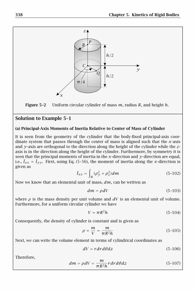
338 Chapter 5. Kinetics of Rigid Bodies
π/4h/2
h/2
x
y
z
C
P
Q
R
Figure 5–2 Uniform circular cylinder of mass m, radius R, and height h.
Solution to Example 5–1
(a) Principal-Axis Moments of Inertia Relative to Center of Mass of Cylinder
It is seen from the geometry of the cylinder that the body-fixed principal-axis coor-dinate system that passes through the center of mass is aligned such that the x-axisand y-axis are orthogonal to the direction along the height of the cylinder while the z-axis is in the direction along the height of the cylinder. Furthermore, by symmetry it isseen that the principal moments of inertia in the x-direction and y-direction are equal,i.e., Ixx = Iyy . First, using Eq. (5–56), the moment of inertia along the x-direction isgiven as
Ixx =∫R(ρ2y + ρ2
z)dm (5–102)
Now we know that an elemental unit of mass, dm, can be written as
dm = ρdV (5–103)
where ρ is the mass density per unit volume and dV is an elemental unit of volume.Furthermore, for a uniform circular cylinder we have
V = πR2h (5–104)
Consequently, the density of cylinder is constant and is given as
ρ = mV= mπR2h
(5–105)
Next, we can write the volume element in terms of cylindrical coordinates as
dV = rdrdθdz (5–106)
Therefore,
dm = ρdV = mπR2h
rdrdθdz (5–107)
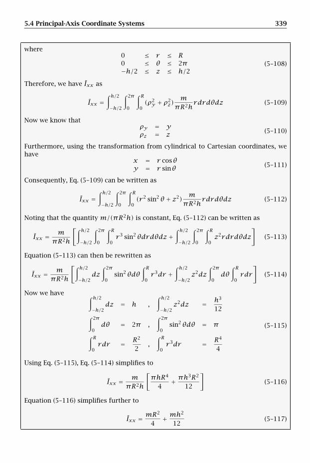
5.4 Principal-Axis Coordinate Systems 339
where0 ≤ r ≤ R0 ≤ θ ≤ 2π−h/2 ≤ z ≤ h/2
(5–108)
Therefore, we have Ixx as
Ixx =∫ h/2−h/2
∫ 2π
0
∫ R0(ρ2y + ρ2
z)mπR2h
rdrdθdz (5–109)
Now we know thatρy = yρz = z (5–110)
Furthermore, using the transformation from cylindrical to Cartesian coordinates, wehave
x = r cosθy = r sinθ (5–111)
Consequently, Eq. (5–109) can be written as
Ixx =∫ h/2−h/2
∫ 2π
0
∫ R0(r 2 sin2θ + z2)
mπR2h
rdrdθdz (5–112)
Noting that the quantity m/(πR2h) is constant, Eq. (5–112) can be written as
Ixx = mπR2h
[∫ h/2−h/2
∫ 2π
0
∫ R0r 3 sin2θdrdθdz +
∫ h/2−h/2
∫ 2π
0
∫ R0z2rdrdθdz
](5–113)
Equation (5–113) can then be rewritten as
Ixx = mπR2h
[∫ h/2−h/2
dz∫ 2π
0sin2θdθ
∫ R0r 3dr +
∫ h/2−h/2
z2dz∫ 2π
0dθ
∫ R0rdr
](5–114)
Now we have ∫ h/2−h/2
dz = h ,∫ h/2−h/2
z2dz = h3
12∫ 2π
0dθ = 2π ,
∫ 2π
0sin2θdθ = π
∫ R0rdr = R2
2,∫ R
0r 3dr = R4
4
(5–115)
Using Eq. (5–115), Eq. (5–114) simplifies to
Ixx = mπR2h
[πhR4
4+ πh
3R2
12
](5–116)
Equation (5–116) simplifies further to
Ixx = mR2
4+ mh
2
12(5–117)

340 Chapter 5. Kinetics of Rigid Bodies
Rewriting Eq. (5–117), we obtain Ixx as
Ixx = m(3R2 + h2)
12(5–118)
Using the fact that Iyy = Ixx , we have
Iyy = m(3R2 + h2)
12(5–119)
Next, the moment of inertia relative to the center of mass of the cylinder about thez-direction is given as
Izz =∫R(ρ2x + ρ2
y)dm (5–120)
Now we haveρx = xρy = y (5–121)
Furthermore, using Eq. (5–110), we have that
ρ2x + ρ2
y = x2 +y2 = (r cosθ)2 + (r sinθ)2 = r 2 (5–122)
Equation (5–120) can then be written as
Izz =∫Rr 2dm (5–123)
Using dm from Eq. (5–107) and the limits of integration from Eq. (5–108), we have
Izz =∫ h/2−h/2
∫ 2π
0
∫ R0
mπR2h
r 3drdθdz (5–124)
Rearranging Eq. (5–124), we obtain
Izz = mπR2h
∫ h/2−h/2
dz∫ 2π
0dθ
∫ R0r 3dr (5–125)
Then, using the results of Eq. (5–115), we have that
Izz = mπR2h
h(2π)R4
4(5–126)
Equation (5–126) simplifies to
Izz = 12mR2 (5–127)
The moments of inertia Ixx , Iyy and Izz are then given as
Ixx = m(3R2 + h2)12
(5–128)
Iyy = m(3R2 + h2)12
(5–129)
Izz = mR2
2(5–130)
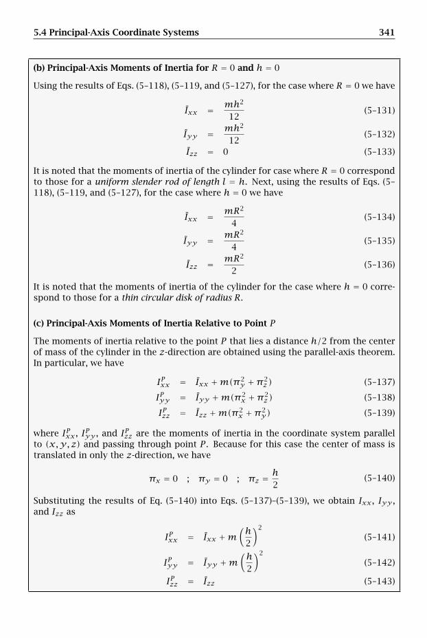
5.4 Principal-Axis Coordinate Systems 341
(b) Principal-Axis Moments of Inertia for R = 0 and h = 0
Using the results of Eqs. (5–118), (5–119, and (5–127), for the case where R = 0 we have
Ixx = mh2
12(5–131)
Iyy = mh2
12(5–132)
Izz = 0 (5–133)
It is noted that the moments of inertia of the cylinder for case where R = 0 correspondto those for a uniform slender rod of length l = h. Next, using the results of Eqs. (5–118), (5–119, and (5–127), for the case where h = 0 we have
Ixx = mR2
4(5–134)
Iyy = mR2
4(5–135)
Izz = mR2
2(5–136)
It is noted that the moments of inertia of the cylinder for the case where h = 0 corre-spond to those for a thin circular disk of radius R.
(c) Principal-Axis Moments of Inertia Relative to Point P
The moments of inertia relative to the point P that lies a distance h/2 from the centerof mass of the cylinder in the z-direction are obtained using the parallel-axis theorem.In particular, we have
IPxx = Ixx +m(π2y +π2
z ) (5–137)
IPyy = Iyy +m(π2x +π2
z ) (5–138)
IPzz = Izz +m(π2x +π2
y) (5–139)
where IPxx , IPyy , and IPzz are the moments of inertia in the coordinate system parallelto (x,y, z) and passing through point P . Because for this case the center of mass istranslated in only the z-direction, we have
πx = 0 ; πy = 0 ; πz = h2 (5–140)
Substituting the results of Eq. (5–140) into Eqs. (5–137)–(5–139), we obtain Ixx , Iyy ,and Izz as
IPxx = Ixx +m(h2
)2
(5–141)
IPyy = Iyy +m(h2
)2
(5–142)
IPzz = Izz (5–143)
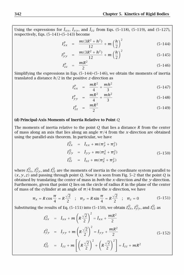
342 Chapter 5. Kinetics of Rigid Bodies
Using the expressions for Ixx , Iyy , and Izz from Eqs. (5–118), (5–119), and (5–127),respectively, Eqs. (5–141)–(5–143) become
IPxx = m(3R2 + h2)12
+m(h2
)2
(5–144)
IPyy = m(3R2 + h2)12
+m(h2
)2
(5–145)
IPzz = mR2
2(5–146)
Simplifying the expressions in Eqs. (5–144)–(5–146), we obtain the moments of inertiatranslated a distance h/2 in the positive z-direction as
IPxx = mR2
4+ mh
2
3(5–147)
IPyy = mR2
4+ mh
2
3(5–148)
IPzz = mR2
2(5–149)
(d) Principal-Axis Moments of Inertia Relative to Point Q
The moments of inertia relative to the point Q that lies a distance R from the centerof mass along an axis that lies along an angle π/4 from the x-direction are obtainedusing the parallel-axis theorem. In particular, we have
IQxx = Ixx +m(π2y +π2
z )
IQyy = Iyy +m(π2x +π2
z )
IQzz = Izz +m(π2x +π2
y)
(5–150)
where IQxx , IQyy , and IQzz are the moments of inertia in the coordinate system parallel to(x,y, z) and passing through point Q. Now it is seen from Fig. 5–2 that the point Q isobtained by translating the center of mass in both the x-direction and the y-direction.Furthermore, given that point Q lies on the circle of radius R in the plane of the centerof mass of the cylinder at an angle of π/4 from the x-direction, we have
πx = R cosπ4= R
√2
2; πy = R sin
π4= R
√2
2; πz = 0 (5–151)
Substituting the results of Eq. (5–151) into (5–150), we obtain IQxx , IQyy , and IQzz as
IQxx = Ixx +m(R√
22
)2
= Ixx + mR2
2
IQyy = Iyy +m(R√
22
)2
= Iyy + mR2
2
IQzz = Izz +m⎡⎣(R
√2
2
)2
+(R√
22
)2⎤⎦ = Izz +mR2
(5–152)
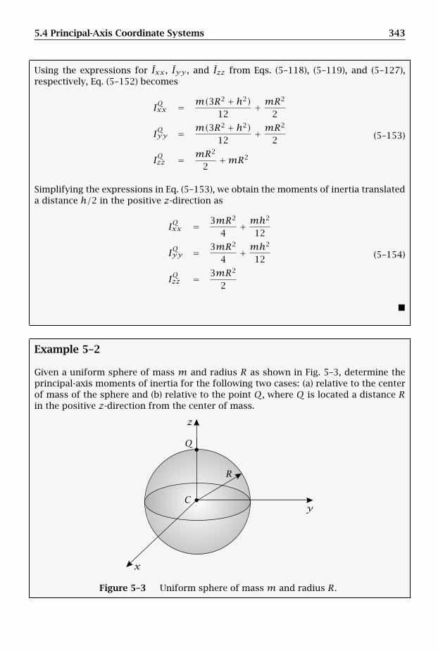
5.4 Principal-Axis Coordinate Systems 343
Using the expressions for Ixx , Iyy , and Izz from Eqs. (5–118), (5–119), and (5–127),respectively, Eq. (5–152) becomes
IQxx = m(3R2 + h2)12
+ mR2
2
IQyy = m(3R2 + h2)12
+ mR2
2
IQzz = mR2
2+mR2
(5–153)
Simplifying the expressions in Eq. (5–153), we obtain the moments of inertia translateda distance h/2 in the positive z-direction as
IQxx = 3mR2
4+ mh
2
12
IQyy = 3mR2
4+ mh
2
12
IQzz = 3mR2
2
(5–154)
Example 5–2
Given a uniform sphere of mass m and radius R as shown in Fig. 5–3, determine theprincipal-axis moments of inertia for the following two cases: (a) relative to the centerof mass of the sphere and (b) relative to the point Q, where Q is located a distance Rin the positive z-direction from the center of mass.
x
y
z
C
Q
R
Figure 5–3 Uniform sphere of mass m and radius R.
344 Chapter 5. Kinetics of Rigid Bodies
Solution to Example 5–2
(a) Principal-Axis Moments of Inertia Relative to Center of Mass of Sphere
It is seen from the geometry of the sphere that the body-fixed principal-axis coordinatesystem that passes through the center of mass is aligned such that all three axes liealong a diameter of the sphere. Furthermore, due to the symmetry of the sphere, it isseen that Ixx = Iyy = Izz. Consequently, it is sufficient to compute one of the momentsof inertia. Using Eq. (5–56), the moment of inertia along the x-direction is given as
Ixx =∫R(ρ2y + ρ2
z)dm (5–155)
We know that an elemental unit of mass, dm, can be written as
dm = ρdV (5–156)
where ρ is the mass density per unit volume and dV is an elemental unit of volume.Furthermore, for a uniform sphere we have
V = 43πR3 (5–157)
Consequently, the density of cylinder is constant and is given as
ρ = mV= m
43πR3
= 3m4πR3
(5–158)
Next, we can write the volume element in terms of spherical coordinates (Thomas andFinney, 2002) as
dV = r 2 sinφdrdθdφ (5–159)
Therefore,
dm = ρdV = 3m4πR3
r 2 sinφdrdθdφ (5–160)
where0 ≤ r ≤ R0 ≤ θ ≤ 2π0 ≤ φ ≤ π
(5–161)
Therefore, we have Ixx as
Ixx =∫ π
0
∫ 2π
0
∫ R0(ρ2y + ρ2
z)3m
4πR3r 2 sinφdrdθdφ (5–162)
Now we know thatρy = yρz = z (5–163)
Furthermore, using the transformation from spherical to Cartesian coordinates asgiven in Eq. (2–241), we have
x = r sinφ cosθy = r sinφ sinθz = r cosφ
(5–164)

5.4 Principal-Axis Coordinate Systems 345
We have from Eq. (5–164)
ρ2y + ρ2
z = y2 + z2 = r 2 sin2φ sin2θ + r 2 cos2φ = r 2(sin2φ sin2θ + cos2φ) (5–165)
Then, using the fact that sin2φ+ cos2φ = 1, Eq. (5–165) can be rewritten as
ρ2y + ρ2
z = r 2(sin2θ + cos2φ cos2θ) (5–166)
Equation (5–162) then becomes
Ixx =∫ π
0
∫ 2π
0
∫ R0r 2(sin2θ + cos2φ cos2θ)
3m4πR3
r 2 sinφdrdθdφ (5–167)
Noting that the quantity 3m/(4πR3) is a constant, Eq. (5–167) can be rearranged togive
Ixx = 3m4πR3
∫ π0
∫ 2π
0
∫ R0r 2(sin2θ + cos2φ cos2θ)r 2 sinφdrdθdφ (5–168)
Decomposing Eq. (5–168), we obtain
Ixx = 3m4πR3
∫ π0
∫ 2π
0
∫ R0r 4 sin2θ sinφdrdθdφ
+ 3m4πR3
∫ π0
∫ 2π
0
∫ R0r 4 cos2φ sinφ cos2θdrdθdφ
(5–169)
Decoupling the integrals in Eq. (5–169) gives
Ixx = 3m4πR3
∫ π0
sinφdφ∫ 2π
0sin2θdθ
∫ R0r 4dr
+ 3m4πR3
∫ π0
cos2φ sinφdφ∫ 2π
0cos2θdθ
∫ R0r 4dr
(5–170)
Now we have the following: ∫ π0
sinφdφ = 2
∫ π0
cos2φ sinφdφ = 23∫ 2π
0sin2θdθ = π
∫ 2π
0cos2θdθ = π
∫ R0r 4dr = R5
5
(5–171)
Substituting the results of Eq. (5–171) into (5–170), we obtain
Ixx = 3m4πR3
[2πR5
5+ 2
3πR5
5
](5–172)

346 Chapter 5. Kinetics of Rigid Bodies
Simplifying Eq. (5–172) gives
Ixx = 3mR2
10+ mR
2
10= 4mR2
10= 2mR2
5(5–173)
Finally, due to the symmetry of the sphere, we have
Iyy = Izz = Ixx = 2mR2
5(5–174)
(b) Principal-Axis Moments of Inertia Relative to Point Q
The moments of inertia relative to the point Q that lies a distance R from the center ofmass along the z-direction are obtained using the parallel-axis theorem. In particular,we have
IQxx = Ixx +m(π2y +π2
z )
IQyy = Iyy +m(π2x +π2
z )
IQzz = Izz +m(π2x +π2
y)
(5–175)
where IQxx , IQyy , and IQzz are the moments of inertia in the coordinate system parallel to(x,y, z) and passing through point Q. Now it is seen from Fig. 5–3 that the point Q isobtained by translating the center of mass in only the z-direction. Furthermore, giventhat point Q lies on the circle of radius R and in the plane of the center of mass of thesphere, we have
πx = 0
πy = 0
πz = R(5–176)
Substituting the results of Eq. (5–176) into (5–175), we obtain IQxx , IQyy , and IQzz as
IQxx = Ixx +mR2
IQyy = Iyy +mR2
IQzz = Izz
(5–177)
Using the expressions for Ixx , Iyy , and Izz from Eqs. (5–173) and (5–174), respectively,Eq. (5–177) becomes
IQxx = 2mR2
5+mR2
IQyy = 2mR2
5+mR2
IQzz = 2mR2
5
(5–178)
5.4 Principal-Axis Coordinate Systems 347
Simplifying the expressions in Eq. (5–178), we obtain the moments of inertia translateda distance R in the positive z-direction as
IQxx = 7mR2
5
IQyy = 7mR2
5
IQzz = 2mR2
5
(5–179)
Example 5–3
Consider a rigid body R whose moment of inertia tensor relative to the center of massof R is given as
IR = 14e1 ⊗ e1 − 4e1 ⊗ e2 − 2e1 ⊗ e3
− 4e2 ⊗ e1 + 14e2 ⊗ e2 − 2e2 ⊗ e3
− 2e3 ⊗ e1 − 2e3 ⊗ e2 + 12e3 ⊗ e3
where e1,e2,e3 is a basis fixed in R. Determine (a) the principal moments of inertia,(b) a principal-axis basis Ep = ep1 ,ep2 ,ep3 of R in terms of the body-fixed basis E =e1,e2,e3, and (c) the moment of inertia tensor in terms of the principal-axis basisEp = ep1 ,ep2 ,ep3 .
Solution to Example 5–3
First, let E = e1,e2,e3. Then, the matrix representation of IR
in the basis E is givenas
IR
E=
⎧⎪⎨⎪⎩
14 −4 −2−4 14 −2−2 −2 12
⎫⎪⎬⎪⎭ (5–180)
Furthermore, from Eq. (5–89) the eigenvalues of the matrixIR
Eare obtained by solv-
ing for the roots of the equation
det
⎧⎪⎨⎪⎩
14− I −4 −2−4 14− I −2−2 −2 12− I
⎫⎪⎬⎪⎭ = 0 (5–181)
Expanding the determinant in Eq. (5–181) and setting the result equal to zero, weobtain the following cubic polynomial in I:
I3 − 40I2 + 508I − 2016 = 0 (5–182)

348 Chapter 5. Kinetics of Rigid Bodies
Computing the roots of the cubic polynomial in Eq. (5–182), we have
I1 = 8I2 = 14I3 = 18
(5–183)
The values I1, I2, and I3 are the principal-axis moments of inertia of the rigid body R.Suppose now that we let ep1 , ep2 , and ep3 be the eigenvectors of the tensor I
R. Then,
after some algebra, the column-vector representations of the eigenvectors in the basisE = e1,e2,e3 are given, respectively, as
ep1
E=
⎧⎪⎪⎨⎪⎪⎩
1√3
1√3
1√3
⎫⎪⎪⎬⎪⎪⎭ (5–184)
ep2
E=
⎧⎪⎪⎨⎪⎪⎩− 1√
6
− 1√6
2√6
⎫⎪⎪⎬⎪⎪⎭ (5–185)
ep3
E=
⎧⎪⎪⎨⎪⎪⎩− 1√
21√2
0
⎫⎪⎪⎬⎪⎪⎭ (5–186)
The eigenvector matrix PEEp is then given as
PEEp =
⎧⎪⎪⎨⎪⎪⎩
1√3 − 1√
6 − 1√2
1√3 − 1√
61√2
1√3
2√6 0
⎫⎪⎪⎬⎪⎪⎭ (5–187)
Correspondingly, the matrix PEpE (which, by definition, is the transpose of the matrix
PEEp because PE
Ep is an orthogonal matrix) is given as
PEpE =
⎧⎪⎪⎨⎪⎪⎩
1√3
1√3
1√3
− 1√6 − 1√
62√6
− 1√2
1√2 0
⎫⎪⎪⎬⎪⎪⎭ (5–188)
Then, computing the quantity PEpE
IRQ
EPE
Ep , we obtain
PEpE
IRQ
EPE
Ep =
⎧⎪⎨⎪⎩
8 0 00 14 00 0 18
⎫⎪⎬⎪⎭ (5–189)
Furthermore, the eigenvectors of the inertia tensor IR
are given as
ep1 = 1√3
e1 + 1√3
e2 + 1√3
e3 (5–190)
ep2 = − 1√6
e1 − 1√6
e2 + 2√6
e3 (5–191)
ep3 = − 1√2
e1 + 1√2
e2 (5–192)
5.5 Actions on a Rigid Body 349
It is noted that the eigenvectors ep1 , ep2 , and ep3 form a principal-axis basis. The moment
of inertia tensor IR
can then be represented in the principal-axis basis Ep = ep1 ,ep2 ,ep3 as
IR = 8ep1 ⊗ ep1 + 14ep2 ⊗ ep2 + 18ep3 ⊗ ep3 (5–193)
5.4.3 Common Usage of Principal-Axis Coordinate Systems
While in principal it is possible to start with a moment of inertia tensor in a non-principal-axis coordinate system and transform to principal-axis coordinates, in thisbook we will restrict our attention to rigid bodies whose principal-axis moments ofinertia (and corresponding principal-axes themselves) are already known. Appendix Aprovides a table of principal-axis moments of inertia relative to the center of mass ofmany common rigid bodies. These shapes will form the basis for many of the examplesconsidered throughout the remainder of this chapter.
As a short aside, it is noted that for most applications a principal-axis coordinatesystem will necessarily be fixed in a rigid body. However, in some (relatively simple)situations it is possible to find a principal-axis coordinate system that is not fixed in arigid body.4 In terms of a principal-axis basis ep1 ,ep2 ,ep3 , the angular momentum ofthe rigid body in an inertial reference frame N relative to a point Q fixed in the bodyis given as
NHQ = IR · NωR = IQ1 ω1ep1 + IQ2 ω2ep2 + IQ3 ω3ep3 (5–194)
where we recall that NωR = ω1ep1 +ω2ep2 +ω3ep3 is the angular velocity of the rigidbody in the inertial reference frame N .
5.5 Actions on a Rigid Body
Because a particle can undergo only translational motion, the only fundamental actionthat can be applied to a particle is that of a force; any moments arise from the ap-plication of a force about a point. However, because a rigid body can undergo bothtranslational and rotational motion, two fundamental actions can be applied to a rigidbody. The first fundamental action that can be applied to a rigid body is the same asthat of a particle, namely, a force. However, in addition to forces, a rigid body can alsobe subjected to a so-called pure torque that affects only the rotational motion of thebody. We now describe the effects that a force and a torque have on a rigid body.
4A homogeneous circular disk is an example of a rigid body for which a principal-axis coordinate systemexists that is not fixed in the body. In this case, because the disk is circular, a principal-axis coordinatesystem can be constructed by choosing the origin to be the center of mass of the disk and choosing thebasis such that one basis vector is orthogonal to the plane of the disk while the other two basis vectorslie in the plane of the disk. In particular, the two basis vectors that lie in the plane of the disk need notbe fixed to the disk (see Example 5–4 for a specific instance of a non-body-fixed principal-axis coordinatesystem).
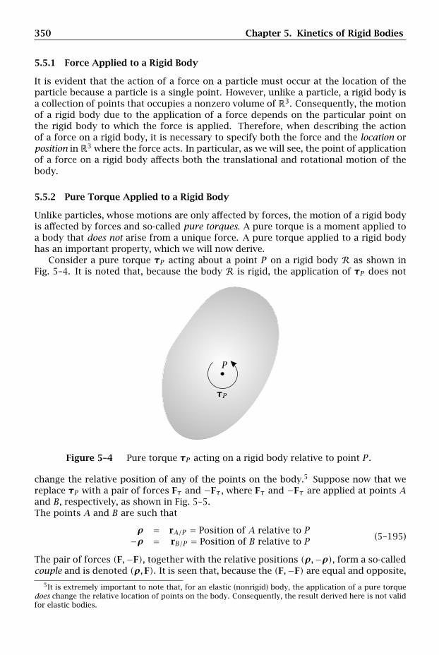
350 Chapter 5. Kinetics of Rigid Bodies
5.5.1 Force Applied to a Rigid Body
It is evident that the action of a force on a particle must occur at the location of theparticle because a particle is a single point. However, unlike a particle, a rigid body isa collection of points that occupies a nonzero volume of R3. Consequently, the motionof a rigid body due to the application of a force depends on the particular point onthe rigid body to which the force is applied. Therefore, when describing the actionof a force on a rigid body, it is necessary to specify both the force and the location orposition in R3 where the force acts. In particular, as we will see, the point of applicationof a force on a rigid body affects both the translational and rotational motion of thebody.
5.5.2 Pure Torque Applied to a Rigid Body
Unlike particles, whose motions are only affected by forces, the motion of a rigid bodyis affected by forces and so-called pure torques. A pure torque is a moment applied toa body that does not arise from a unique force. A pure torque applied to a rigid bodyhas an important property, which we will now derive.
Consider a pure torque τP acting about a point P on a rigid body R as shown inFig. 5–4. It is noted that, because the body R is rigid, the application of τP does not
P
τP
Figure 5–4 Pure torque τP acting on a rigid body relative to point P .
change the relative position of any of the points on the body.5 Suppose now that wereplace τP with a pair of forces Fτ and −Fτ , where Fτ and −Fτ are applied at points Aand B, respectively, as shown in Fig. 5–5.The points A and B are such that
ρ = rA/P = Position of A relative to P−ρ = rB/P = Position of B relative to P (5–195)
The pair of forces (F,−F), together with the relative positions (ρ,−ρ), form a so-calledcouple and is denoted (ρ,F). It is seen that, because the (F,−F) are equal and opposite,
5It is extremely important to note that, for an elastic (nonrigid) body, the application of a pure torquedoes change the relative location of points on the body. Consequently, the result derived here is not validfor elastic bodies.
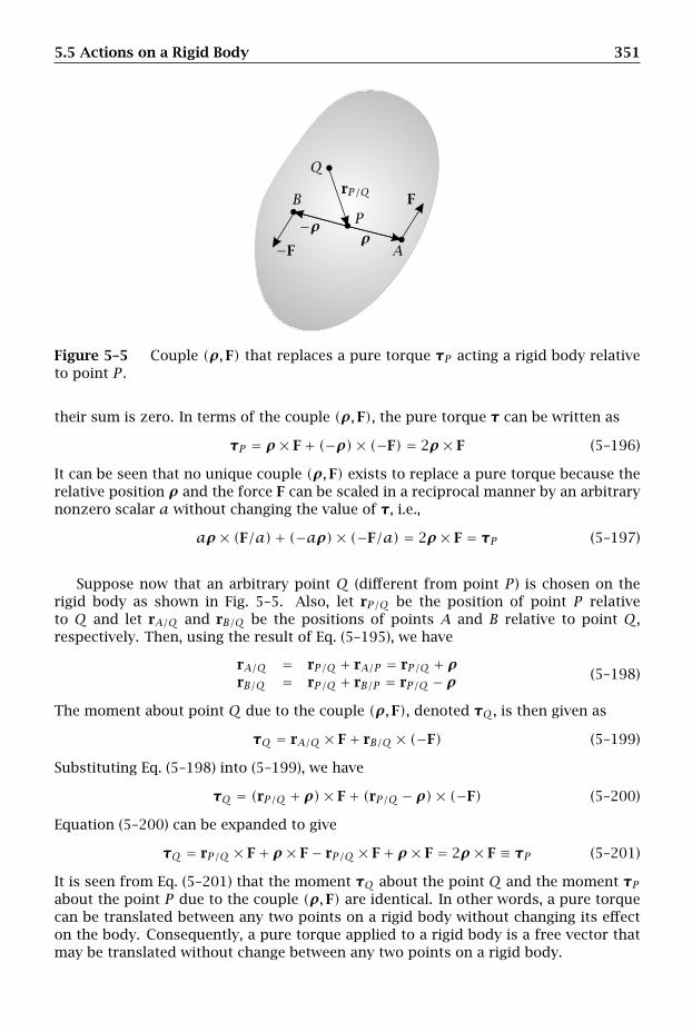
5.5 Actions on a Rigid Body 351
F
−F
rP/Q
A
BP
Q
ρ−ρ
Figure 5–5 Couple (ρ,F) that replaces a pure torque τP acting a rigid body relativeto point P .
their sum is zero. In terms of the couple (ρ,F), the pure torque τ can be written as
τP = ρ× F+ (−ρ)× (−F) = 2ρ× F (5–196)
It can be seen that no unique couple (ρ,F) exists to replace a pure torque because therelative position ρ and the force F can be scaled in a reciprocal manner by an arbitrarynonzero scalar a without changing the value of τ, i.e.,
aρ× (F/a)+ (−aρ)× (−F/a) = 2ρ× F = τP (5–197)
Suppose now that an arbitrary point Q (different from point P ) is chosen on therigid body as shown in Fig. 5–5. Also, let rP/Q be the position of point P relativeto Q and let rA/Q and rB/Q be the positions of points A and B relative to point Q,respectively. Then, using the result of Eq. (5–195), we have
rA/Q = rP/Q + rA/P = rP/Q + ρrB/Q = rP/Q + rB/P = rP/Q − ρ (5–198)
The moment about point Q due to the couple (ρ,F), denoted τQ, is then given as
τQ = rA/Q × F+ rB/Q × (−F) (5–199)
Substituting Eq. (5–198) into (5–199), we have
τQ = (rP/Q + ρ)× F+ (rP/Q − ρ)× (−F) (5–200)
Equation (5–200) can be expanded to give
τQ = rP/Q × F+ ρ× F− rP/Q × F+ ρ× F = 2ρ× F ≡ τP (5–201)
It is seen from Eq. (5–201) that the moment τQ about the point Q and the moment τPabout the point P due to the couple (ρ,F) are identical. In other words, a pure torquecan be translated between any two points on a rigid body without changing its effecton the body. Consequently, a pure torque applied to a rigid body is a free vector thatmay be translated without change between any two points on a rigid body.
352 Chapter 5. Kinetics of Rigid Bodies
5.5.3 Power and Work of a Pure Torque
Suppose that τ is a pure torque acting on a rigid bodyR. Furthermore, let NωR be theangular velocity of R in an inertial reference frame N . Then the power produced by τin reference frame N is defined as
NPτ = τ · NωR (5–202)
Furthermore, the work of a pure torque on the time interval from t1 to t2 in referenceframe N is given as
NWτ =∫ t2t1
NPτdt =∫ t2t1τ · NωRdt (5–203)
5.5.4 Conservative Torques
As with a force applied to a particle or a rigid body, the work done by a pure torqueover a time interval t ∈ [t1, t2] in rotating a rigid body between two orientations willdepend on both the trajectory taken by the particle on [t1, t2] and the orientationsof the rigid body at the endpoints t1 and t2. Suppose now that we let Θ ∈ R3 be acolumn-vector whose elements describe the orientation of a rigid body R in an inertialreference frame N , i.e., Θ is given as
Θ =
⎧⎪⎨⎪⎩θ1
θ2
θ3
⎫⎪⎬⎪⎭ (5–204)
Then a torque τc is said to be conservative if the work done in rotating the rigidbody from an initial orientation Θ1 at t = t1 to a final orientation Θ2 at t = t2 isindependent of the trajectory taken to rotate the rigid body fromΘ(t1) = Θ1 toΘ(t2) =Θ2. In other words, if
[NωR](1) , . . . , [NωR](n) are the angular velocities in an inertialreference frame N that correspond to an arbitrary set of n trajectories that startat Θ1 and end at Θ2, then the pure torque τc is conservative if, for all trajectories[NωR](1) , . . . , [NωR](n), (i = 1,2, . . . , n), we have
NWτc12 =∫ t2t1τc ·
[NωR
](1)dt = · · · =
∫ t2t1τc ·
[NωR
](n)dt (5–205)
A consequence of the fact that a conservative torque is independent of the trajectoryis that there exists a scalar function NV = NV(Θ) such that
τc = −∇ΘNV = − ∂∂Θ
(NV
)(5–206)
The power of a conservative torque can then be written as
NPcτ = τc · NωR = −∇ΘNV · NωR (5–207)
Now, as was seen in Chapter 2, the orientation of a rigid body cannot be obtainedvia direct integration of the angular velocity. As a result, an alternate parameterizationof the orientation of the rigid body was developed using Euler angles. In particular, in
5.6 Moment Transport Theorem for a Rigid Body 353
terms of Type I Euler angles, it was shown in Eq. (2–600) on page 120 that the angularvelocity of a rigid body R in an arbitrary reference frame A can be written in terms ofthe Euler basis (O’Reilly and Srinivasa, 2002) as
AωR = ψk1 + θk2 + φk3 (5–208)
where ψ, θ, and φ are the set of Type I Euler angles and k1,k2,k3 is the correspond-ing Euler basis. Using the expression for AωR in Eq. (5–208) and the definition of thepower of a conservative torque from Eq. (5–207), we can write
τc · NωR = −∇ΘNV ·(ψk1 + θk2 + φk3
)(5–209)
Furthermore, we can obtain a second expression for τc ·NωR by noting that the powerof τc can be obtained by computing the rate of change of NV as
NPτ = − ddt(NV
)= − ∂
∂ψ
(NV
)ψ− ∂
∂θ
(NV
)θ − ∂
∂φ
(NV
)φ (5–210)
Now, in order for the expressions in Eqs. (5–209) and (5–210) to be equal, it is necessaryto determine a basis to express ∇ΘNV such that the scalar product of ∇ΘNV withNωR equals the expression in Eq. (5–210). In other words, we seek a basis u1,u2,u3such that
∇ΘNV = ∂∂ψ
(NV
)u1 + ∂
∂θ
(NV
)u2 + ∂
∂φ
(NV
)u3 (5–211)
and
∇ΘNV · NωR = ∂∂ψ
(NV
)ψ+ ∂
∂θ
(NV
)θ + ∂
∂φ
(NV
)φ (5–212)
Recall now the dual Euler basis (O’Reilly and Srinivasa, 2002; O’Reilly, 2004) k∗1 ,k∗2 ,k∗3 which, from Eq. (2–601) on page 120, has the property that
k∗i · kj =
1 , i = j0 , i ≠ j (i, j = 1,2,3) (5–213)
Using the property of Eq. (5–213), it is seen that ∇ΘNV can be written in terms of thedual Euler basis as
∇ΘNV = ∂∂ψ
(NV
)k∗1 +
∂∂θ
(NV
)k∗2 +
∂∂φ
(NV
)k∗3 (5–214)
Equation (5–214) is an expression for the gradient of the potential energy of a conser-vative pure torque in terms of Type I Euler angles expressed in the Type I dual Eulerbasis. Using Eq. (5–214), the conservative torque is given in terms of Type I Euler anglesand the corresponding dual Euler basis as
τc = − ∂∂ψ
(NV
)k∗1 −
∂∂θ
(NV
)k∗2 −
∂∂φ
(NV
)k∗3 (5–215)
5.6 Moment Transport Theorem for a Rigid Body
Let F1, . . . ,Fn be the forces that act on a rigid body R. Furthermore, let r1, . . . , rn bethe positions of the forces F1, . . . ,Fn, respectively. Finally, let τ be the resultant pure
354 Chapter 5. Kinetics of Rigid Bodies
torque acting on R. Then the resultant moment applied to R relative to an arbitrarypoint Q is defined as
MQ =n∑i=1
(ri − rQ)× Fi + τ (5–216)
Furthermore, the resultant moment applied to R relative to a point O fixed in aninertial reference frame is defined as
MO =n∑i=1
(ri − rO)× Fi + τ (5–217)
Lastly, the resultant moment applied toR relative to the center of mass ofR is definedas
M =n∑i=1
(ri − r)× Fi + τ (5–218)
It is seen that the pure torque in Eqs. (5–216), (5–217), and (5–218) is the same due tothe fact that a pure torque τ is a free vector and thus can be translated to any pointon a rigid body without change.
Suppose now that we choose a second arbitrary point Q′. Then, from Eq. (5–216),the moment due to all forces and all pure torques relative to Q′ is given as
MQ′ =n∑i=1
(ri − rQ′)× Fi + τ (5–219)
Subtracting Eq. (5–216) from (5–219), we have
MQ′ −MQ =n∑i=1
(rQ − rQ′)× Fi (5–220)
Observing that rQ and rQ′ are independent of the summation, Eq. (5–220) can be writ-ten as
MQ′ −MQ = (rQ − rQ′)×n∑i=1
Fi (5–221)
Now we recall that
F =n∑i=1
Fi (5–222)
Therefore, Eq. (5–221) becomes
MQ′ −MQ = (rQ − rQ′)× F (5–223)
Rearranging Eq. (5–223), we obtain
MQ′ = MQ + (rQ − rQ′)× F (5–224)
Equation (5–224) is called the moment transport theorem for a rigid body and can beused to determine the moment applied to a rigid body relative to a point Q′ when themoment applied relative to a point Q is already known.
5.7 Euler’s Laws for a Rigid Body 355
5.7 Euler’s Laws for a Rigid Body
Because a rigid body has both translational and rotational motion, two independentbalance laws are required to fully specify the motion of the body. In particular, onebalance law is needed to describe the translational motion and another law is neededto describe the rotational motion of the rigid body. These two balance laws for a rigidbody are called Euler’s laws. We now state Euler’s laws.
5.7.1 Euler’s 1st Law:
The resultant force applied to a rigid body R is equal to the product of the mass of therigid body and the acceleration of the center of mass of the rigid body in an inertialreference frame N , i.e.,
F =mNa (5–225)
5.7.2 Euler’s 2nd Law:
The resultant moment applied to a rigid body R relative to a point O fixed point in aninertial reference frame N is equal to the rate of change of angular momentum of therigid body relative to point O in reference frame N , i.e.,
MO =Nddt
(NHO
)(5–226)
5.7.3 Alternate Forms of Euler’s 2nd Law
Because of its simplicity, it is most desirable to apply Euler’s 2nd law about an inertiallyfixed point. However, for many problems it is difficult to find a convenient inertiallyfixed point about which to apply Euler’s 2nd law. For such situations, it is important tohave ways to apply Euler’s 2nd law relative to a point that moves relative to any inertialreference frame. In this section we develop two alternate forms of Euler’s 2nd law. Thefirst is applicable relative to an arbitrary reference point while the second is applicablerelative to the center of mass of the rigid body.
Euler’s 2nd Law Relative to an Arbitrary Reference Point
Recalling Eq. (5–21), the relationship between the angular momentum of a rigid bodyin an inertial reference frame N relative to an arbitrary reference point Q, NHQ, andthe angular of a rigid body in an inertial reference frame N relative to a point O fixedin N , NHQ, is given as
NHQ = NHO + (r− rQ)×m(Nv−NvQ)− (r− rO)×mNv (5–227)
Computing the rate of change of NHQ in Eq. (5–227) in reference frame N , we have
Nddt
(NHQ
)=Nddt
(NHO
)+ (Nv−NvQ)×m(Nv−NvQ)
+ (r− rQ)×m(Na−NaQ)−Nv×mNv− (r− rO)×mNa(5–228)
356 Chapter 5. Kinetics of Rigid Bodies
Now we observe that the second and fourth terms in Eq. (5–228) are zero. Therefore,Eq. (5–228) simplifies to
Nddt
(NHQ
)=Nddt
(NHO
)+ (r− rQ)×m(Na−NaQ)− (r− rO)×mNa (5–229)
Then, applying Euler’s 2nd law from Eq. (5–226), the expression in Eq. (5–229) becomes
Nddt
(NHQ
)= MO + (r− rQ)×m(Na−NaQ)− (r− rO)×mNa (5–230)
Furthermore, applying the moment transport theorem of Eq. (5–224), we have
MO = MQ + (rQ − rO)× F (5–231)
Substituting the result of Eq. (5–231) into (5–230) gives
Nddt
(NHQ
)= MQ + (rQ − rO)× F+ (r− rQ)×m(Na−NaQ)− (r− rO)×mNa (5–232)
Then, applying Euler’s 1st law from Eq. (5–225), the expression in Eq. (5–232) can bewritten asNddt
(NHQ
)= MQ+(rQ−rO)×mNa+ (r−rQ)×m(Na−NaQ)− (r−rO)×mNa (5–233)
Equation (5–233) simplifies to
MQ − (r− rQ)×mNaQ =Nddt
(NHQ
)(5–234)
It is observed that, similar to the result for a system of particles, the quantity
−(r− rQ)×mNaQ
is the inertial moment of the reference point Q relative to the center of mass of thesystem. From Eq. (5–234), we obtain the following statement of Euler’s 2nd law relativeto an arbitrary reference point:
The sum of the resultant moment applied to a rigid body relative to an arbitrary refer-ence point Q and the inertial moment due to the acceleration of the reference point Qrelative to the center of mass of a rigid body is equal to the rate of change of angularmomentum of the rigid body relative to the reference point Q, i.e.,
MQ − (r− rQ)×mNaQ =Nddt
(NHQ
)(5–235)
Euler’s 2nd Law Relative to the Center of Mass
Suppose that we choose the reference point in Eq. (5–234) to be the center of mass ofthe rigid body. Then rQ = r, which implies that (r − rQ) ×mNaQ = 0. Furthermore,MQ = M, and Eq. (5–234) simplifies to
M =Nddt
(NH)
(5–236)
5.7 Euler’s Laws for a Rigid Body 357
From Eq. (5–236), we obtain the following statement of Euler’s 2nd law relative to thecenter of mass of a rigid body:
The resultant moment applied to a rigid body about its center of mass is equal to therate of change of angular momentum of the rigid body relative to its center of mass,i.e.,
M =Nddt
(NH)
(5–237)
5.7.4 Important Results About Euler’s 2nd Law
In the previous section, two important results were obtained regarding Euler’s 2nd lawfor a rigid body. First, it is noted that the relationship
M =Nddt
(NH
)(5–238)
is valid only when the reference point is fixed in an inertial reference frame or is thecenter of mass of a rigid body. However, if an arbitrary reference point (i.e., a referencepoint that is neither a point fixed in an inertial reference frame nor the center of massof the rigid body), then the rate of change of angular momentum is not equal to theresultant moment. Instead, in the latter case of an arbitrary reference pointQ, we have
MQ − (r− rQ)×mNaQ =Nddt
(NHQ
)(5–239)
where −(r−rQ)×mNaQ is the inertial moment of the reference point Q relative to thecenter of mass of the system. It is important to re-emphasize that Eq. (5–239) must beapplied when neither a fixed point nor the center of mass of the system is convenientfor performing the analysis.
Example 5–4
A uniform circular cylinder of massm and radius r rolls along a fixed plane inclined ata constant inclination angle β with the horizontal as shown in Fig. 5–6. Knowing thatgravity acts downward, determine the differential equation of motion for the cylinderin terms of the angle θ using the following reference points: (a) the center of mass ofthe cylinder; (b) the instantaneous point of contact fixed to the cylinder; and (c) theinstantaneous point of contact that moves parallel to the center of mass in a straightline down the incline.
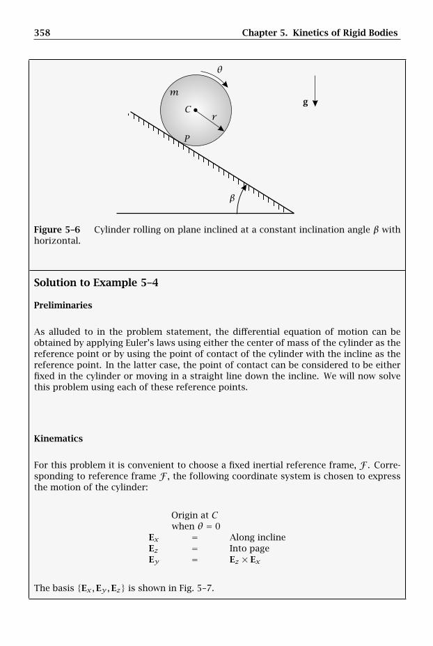
358 Chapter 5. Kinetics of Rigid Bodies
gm
rC
P
β
θ
Figure 5–6 Cylinder rolling on plane inclined at a constant inclination angle β withhorizontal.
Solution to Example 5–4
Preliminaries
As alluded to in the problem statement, the differential equation of motion can beobtained by applying Euler’s laws using either the center of mass of the cylinder as thereference point or by using the point of contact of the cylinder with the incline as thereference point. In the latter case, the point of contact can be considered to be eitherfixed in the cylinder or moving in a straight line down the incline. We will now solvethis problem using each of these reference points.
Kinematics
For this problem it is convenient to choose a fixed inertial reference frame, F . Corre-sponding to reference frame F , the following coordinate system is chosen to expressthe motion of the cylinder:
Origin at Cwhen θ = 0
Ex = Along inclineEz = Into pageEy = Ez × Ex
The basis Ex,Ey,Ez is shown in Fig. 5–7.
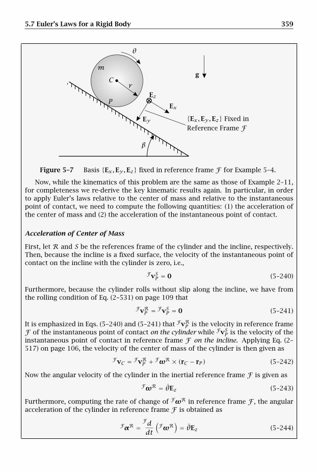
5.7 Euler’s Laws for a Rigid Body 359
Ex,Ey,Ez Fixed inReference Frame F
⊗Ex
Ey
Ez
gm
rC
P
β
θ
Figure 5–7 Basis Ex,Ey,Ez fixed in reference frame F for Example 5–4.
Now, while the kinematics of this problem are the same as those of Example 2–11,for completeness we re-derive the key kinematic results again. In particular, in orderto apply Euler’s laws relative to the center of mass and relative to the instantaneouspoint of contact, we need to compute the following quantities: (1) the acceleration ofthe center of mass and (2) the acceleration of the instantaneous point of contact.
Acceleration of Center of Mass
First, let R and S be the references frame of the cylinder and the incline, respectively.Then, because the incline is a fixed surface, the velocity of the instantaneous point ofcontact on the incline with the cylinder is zero, i.e.,
FvSP = 0 (5–240)
Furthermore, because the cylinder rolls without slip along the incline, we have fromthe rolling condition of Eq. (2–531) on page 109 that
FvRP = FvSP = 0 (5–241)
It is emphasized in Eqs. (5–240) and (5–241) that FvRP is the velocity in reference frameF of the instantaneous point of contact on the cylinder while FvSP is the velocity of theinstantaneous point of contact in reference frame F on the incline. Applying Eq. (2–517) on page 106, the velocity of the center of mass of the cylinder is then given as
FvC = FvRP + FωR × (rC − rP ) (5–242)
Now the angular velocity of the cylinder in the inertial reference frame F is given as
FωR = θEz (5–243)
Furthermore, computing the rate of change of FωR in reference frame F , the angularacceleration of the cylinder in reference frame F is obtained as
FαR =Fddt
(FωR
)= θEz (5–244)
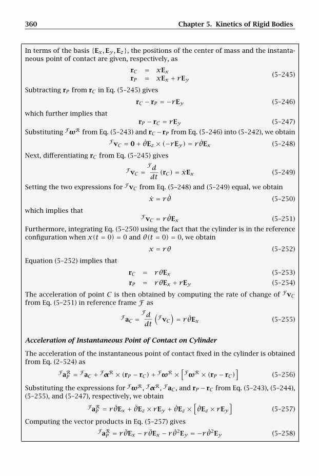
360 Chapter 5. Kinetics of Rigid Bodies
In terms of the basis Ex,Ey,Ez, the positions of the center of mass and the instanta-neous point of contact are given, respectively, as
rC = xExrP = xEx + rEy
(5–245)
Subtracting rP from rC in Eq. (5–245) gives
rC − rP = −rEy (5–246)
which further implies thatrP − rC = rEy (5–247)
Substituting FωR from Eq. (5–243) and rC −rP from Eq. (5–246) into (5–242), we obtainFvC = 0+ θEz × (−rEy) = r θEx (5–248)
Next, differentiating rC from Eq. (5–245) gives
FvC =Fddt(rC) = xEx (5–249)
Setting the two expressions for FvC from Eq. (5–248) and (5–249) equal, we obtain
x = r θ (5–250)
which implies thatFvC = r θEx (5–251)
Furthermore, integrating Eq. (5–250) using the fact that the cylinder is in the referenceconfiguration when x(t = 0) = 0 and θ(t = 0) = 0, we obtain
x = rθ (5–252)
Equation (5–252) implies that
rC = rθEx (5–253)
rP = rθEx + rEy (5–254)
The acceleration of point C is then obtained by computing the rate of change of FvCfrom Eq. (5–251) in reference frame F as
FaC =Fddt
(FvC
)= r θEx (5–255)
Acceleration of Instantaneous Point of Contact on Cylinder
The acceleration of the instantaneous point of contact fixed in the cylinder is obtainedfrom Eq. (2–524) as
FaRP = FaC + FαR × (rP − rC)+ FωR ×[FωR × (rP − rC)
](5–256)
Substituting the expressions for FωR, FαR, FaC , and rP − rC from Eq. (5–243), (5–244),(5–255), and (5–247), respectively, we obtain
FaRP = r θEx + θEz × rEy + θEz ×[θEz × rEy
](5–257)
Computing the vector products in Eq. (5–257) givesFaRP = r θEx − r θEx − r θ2Ey = −r θ2Ey (5–258)
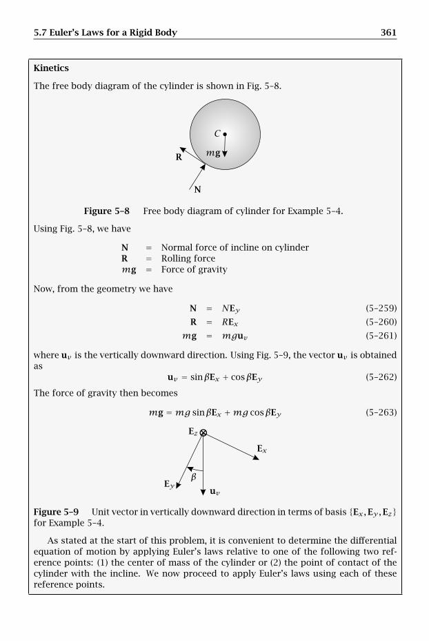
5.7 Euler’s Laws for a Rigid Body 361
Kinetics
The free body diagram of the cylinder is shown in Fig. 5–8.
N
R mg
C
Figure 5–8 Free body diagram of cylinder for Example 5–4.
Using Fig. 5–8, we have
N = Normal force of incline on cylinderR = Rolling forcemg = Force of gravity
Now, from the geometry we have
N = NEy (5–259)
R = REx (5–260)
mg = mguv (5–261)
where uv is the vertically downward direction. Using Fig. 5–9, the vector uv is obtainedas
uv = sinβEx + cosβEy (5–262)
The force of gravity then becomes
mg =mg sinβEx +mg cosβEy (5–263)
⊗Ex
Ey
Ez
uv
β
Figure 5–9 Unit vector in vertically downward direction in terms of basis Ex,Ey,Ezfor Example 5–4.
As stated at the start of this problem, it is convenient to determine the differentialequation of motion by applying Euler’s laws relative to one of the following two ref-erence points: (1) the center of mass of the cylinder or (2) the point of contact of thecylinder with the incline. We now proceed to apply Euler’s laws using each of thesereference points.
362 Chapter 5. Kinetics of Rigid Bodies
(a) Differential Equation Using Center of Mass of Cylinder as Reference Point
Using the center of mass of the cylinder as a reference point, we need to apply both ofEuler’s laws. Recalling Euler’s 1st law from Eq. (5–225), we have
F =mFa (5–264)
Examining the free body diagram of Fig. 5–8, we see that the resultant force acting onthe cylinder is given as
F = R+N+mg (5–265)
Using the expressions for the forces in Eqs. (5–259)–(5–261), we have
F = REx +NEy +mg sinβEx +mg cosβEy (5–266)
Then, noting that Fa = FaC and using the expression FaC from Eq. (5–255), we canequate F and mFa to give
REx +NEy +mg sinβEx +mg cosβEy =mrθEx (5–267)
Rearranging Eq. (5–267), we obtain
(R +mg sinβ)Ex + (N +mg cosβ)Ey =mrθEx (5–268)
Equation (5–268) yields the following two scalar equations:
mrθ = R +mg sinβ (5–269)
0 = N +mg cosβ (5–270)
Recalling Euler’s 2nd about the center of mass of a rigid body from Eq. (5–237), wehave
M =Nddt
(NH)
(5–271)
Examining the free body diagram of Fig. 5–8, we see that the forces mg and N passthrough the center of mass of the cylinder. Consequently, only the rolling force Rproduces a moment about the center of mass of the cylinder. Therefore, the momentrelative to the center of mass of the cylinder is given as
M = (rR − r)× R (5–272)
Now we observe that because the force R acts at the point of contact, we have
rR = rP = rθEx + rEy (5–273)
where we have used the expression for rP from Eq. (5–254). We then have
rR − r = rR − rC = rθEx + rEy − rθEx = rEy (5–274)
Substituting rR from Eq. (5–274) and using the expression for R from Eq. (5–260), weobtain
M = rEy × REx = −rREz (5–275)
5.7 Euler’s Laws for a Rigid Body 363
Also, the angular momentum about the center of mass is given as
FH = I
R · FωR (5–276)
Because the Ex,Ey,Ez is a principal-axis basis, we have
IR = IxxEx ⊗ Ex + IyyEy ⊗ Ey + IzzEz ⊗ Ez (5–277)
Substituting IR
from Eq. (5–277) and FωR from Eq. (5–243), we obtainF
H as
FH = IzzEz ⊗ Ez · θEz = IzzθEz (5–278)
Noting that the moment of inertia of a cylinder about the center of mass along thedirection Ez is Izz =mr 2/2, we have
FH = mr
2
2θEz (5–279)
Computing the rate of change ofF
H in reference frame F , we obtain
Fddt
(FH)= mr
2
2θEz (5–280)
Setting M from Eq. (5–275) equal toF(FH)/dt from Eq. (5–280), we obtain
−rREz = mr2
2θEz (5–281)
which yields the scalar equation
R = −mr2θ (5–282)
The results of Eqs. (5–269) and (5–282) can now be used together to obtain thedifferential equation of motion. Substituting R from Eq. (5–282) into Eq. (5–269) gives
mrθ = −mr2θ +mg sinβ (5–283)
Equation (5–283) can be rearranged to give
3mr2θ =mg sinβ (5–284)
Simplifying Eq. (5–284), we obtain the differential equation of motion as
θ = 2g sinβ3r
(5–285)
(b) Differential Equation Using Instantaneous Point of Contact Fixed in Cylinder asReference Point
A second method to obtain the differential equation of motion is to use the instanta-neous point of contact P between the cylinder and the incline and fixed in the cylinder
364 Chapter 5. Kinetics of Rigid Bodies
as the reference. Now it is seen from Eq. (5–241) that the velocity of the instantaneouspoint of contact fixed in the cylinder is zero. However, from Eq. (5–258) it is seen thatthe acceleration of the instantaneous point of contact is not zero (see Example 2–11for this same result). Consequently, while it may be counterintuitive, the instantaneouspoint of contact of the cylinder with the incline is not a fixed point. Therefore, in orderto use point P as the reference, it is necessary to apply the form of Euler’s 2nd law foran arbitrary reference point as given in Eq. (5–234) on page 356, i.e.,
MP − (rC − rP )×mFaRP =Fddt
(FHP
)(5–286)
Using rC − rP and FaP from Eqs. (5–246) and (5–258), respectively, the inertial momentdue to the acceleration of point P is given as
−(rC − rP )×mFaRP = rEy ×m(−r θ2Ey) = 0 (5–287)
It is seen from Eq. (5–287) that, while P is not a fixed point, the inertial moment due tothe acceleration of point P is zero. This last result arises from the fact that FaRP is inthe same direction as rC − rP .6 Equation (5–286) then simplifies to
MP =Fddt
(FHP
)(5–288)
In other words, for a uniform cylinder that rolls without slip along a flat surface, theinstantaneous point of contact appears to be a fixed point7 and it happens to be the
case that MP is equal toFd(FHP )/dt.
Next, using the free body diagram of Fig. 5–8, it is seen that only the force of gravityproduces a moment relative to point P . Consequently, the moment relative to point Pis given as
MP = (rC − rP )×mg (5–289)
Substituting rC − rP from Eq. (5–246) and mg from Eq. (5–263) into Eq. (5–289), weobtain
MP = −rEy × (mg sinβEx +mg cosβEy) =mgr sinβEz (5–290)
Furthermore, from Eq. (5–24) on page 325, we have
FHP = FHC + (rP − rC)×m(FvRP − FvC) (5–291)
6It is noted that, in the general case of a rigid body rolling on a surface, the acceleration of the point ofcontact fixed in the cylinder, FaRP , would not lie in the same direction as the position of the center of massrelative to the point of contact, rC − rP . In this case the inertial moment of the center of mass relative tothe point of contact, −(rC − rP )×mFaRP , would not be zero.
7For the case of a uniform cylinder rolling on a flat surface, the point of contact P appears to be a fixedpoint because it is the instantaneous center of rotation for the rigid body. While the concept of an in-stantaneous center of rotation can be used on certain simple problems, it is restricted to two-dimensionalmotion. Moreover, even in two dimensions, great care must be taken when using an instantaneous centerof rotation as a reference point. Because of the potential for confusion, instantaneous centers of rotationare not used as the basis for solving problems in this book. See Beer and Johnston (1997), Bedford andFowler (2005), or Greenwood (1988) for discussions about instantaneous centers of rotation.

5.7 Euler’s Laws for a Rigid Body 365
Now, because the cylinder rolls without slip we have FvRP = 0. Consequently,
FvRP − FvC = −FvC = −r θEx (5–292)
SubstitutingF
H, rP − rC , and FvRP − FvC from Eqs. (5–279), (5–247), and (5–292), re-spectively, into Eq. (5–291), we obtain
FHP = mr2
2θEz + rEy ×m(−r θEx) = 3mr 2
2θEz (5–293)
Computing the rate of change of FHP in reference frame F , we obtain
Fddt
(FHP
)= 3mr 2
2θEz (5–294)
Then, setting MP from Eq. (5–290) equal toFd(FHP )/dt from Eq. (5–294), we have
mgr sinβEz = 3mr 2
2θEz (5–295)
Dropping Ez from both sides of Eq. (5–295) and rearranging, we obtain
3mr 2
2θ =mgr sinβ (5–296)
Simplifying Eq. (5–296) yields the differential equation of motion as
θ = 2g sinβ3r
(5–297)
It is seen that the differential equation of Eq. (5–297) obtained using the second methodis identical to that of Eq. (5–285) obtained using the first method.
(c) Differential Equation Using Point of Contact moving in Straight Line Down Inclineas Reference Point
A third method to obtain the differential equation of motion is to use the instantaneouspoint of contact P between the cylinder and the incline and moving in a straight linealong the incline as the reference point. It is important to note in this case that thereference point is not fixed to the cylinder, but rather is the projection of the center ofmass onto the plane of the incline. Now in this case it is seen that point P moves withthe same velocity as the center of mass. Using the expression for the velocity of thecenter of mass in reference frame F from Eq. (5–251), we have
FvP = FvC = r θEx (5–298)
Consequently, the acceleration of point P is given as
FaP =Fddt
(FvP
)= r θEx (5–299)
366 Chapter 5. Kinetics of Rigid Bodies
Again, since FaP ≠ 0, it is seen that point P is not an inertially fixed point. Therefore,it is necessary to apply the general form of Euler’s 2nd law as given in Eq. (5–234) onpage 356, i.e.,
MP − (rC − rP )×mFaP =Fddt
(FHP
)(5–300)
Now we already have MP from Eq. (5–290). Next, using the expressions for rC − rP andFaP from Eqs. (5–246) and (5–299), the inertial moment due to the acceleration of pointP relative to the center of mass of the cylinder is given as
−(rC − rP )×mFaP = −(−rEy)×mrθEx = −mr 2θEz (5–301)
Furthermore, the angular momentum relative to point P is obtained from Eq. (5–24) onpage 325 as
FHP = FHC + (rP − rC)×m(FvP − FvC) (5–302)
Now, from Eq. (5–298), we haveFvP − FvC = 0 (5–303)
The second term in Eq. (5–302) is then zero and Eq. (5–302) reduces to
FHP = FHC = mr2
2θEz (5–304)
where we have used the expression for FHC from Eq. (5–279). Computing the rate ofchange of FHP in Eq. (5–304), we have
Fddt
(FHP
)= mr
2
2θEz (5–305)
Finally, substituting the results of Eqs. (5–290), (5–301), and (5–305) into Eq. (5–300),we obtain
mgr sinβEz −mr 2θEz = mr2
2θEz (5–306)
Dropping the common factor of Ez from both sides of Eq. (5–306) gives
mgr sinβ−mr 2θ = mr2
2θ (5–307)
Rearranging and simplifying Eq. (5–307), we obtain the differential equation of motionas
θ = 2g sinβ3r
(5–308)
It is seen that the differential equation of Eq. (5–308) obtained using this third methodis identical to the results obtained in Eqs. (5–285) and (5–297) using the first and sec-ond methods, respectively.
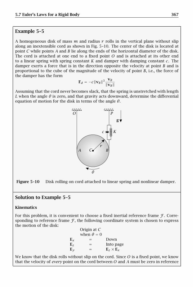
5.7 Euler’s Laws for a Rigid Body 367
Example 5–5
A homogeneous disk of mass m and radius r rolls in the vertical plane without slipalong an inextensible cord as shown in Fig. 5–10. The center of the disk is located atpoint C while points A and B lie along the ends of the horizontal diameter of the disk.The cord is attached at one end to a fixed point O and is attached at its other endto a linear spring with spring constant K and damper with damping constant c. Thedamper exerts a force that is in the direction opposite the velocity at point B and isproportional to the cube of the magnitude of the velocity of point B, i.e., the force ofthe damper has the form
Fd = −c‖vB‖3 vB‖vB‖
Assuming that the cord never becomes slack, that the spring is unstretched with lengthL when the angle θ is zero, and that gravity acts downward, determine the differentialequation of motion for the disk in terms of the angle θ.
c
g
rA BC
K
O P
θ
Figure 5–10 Disk rolling on cord attached to linear spring and nonlinear damper.
Solution to Example 5–5
Kinematics
For this problem, it is convenient to choose a fixed inertial reference frame F . Corre-sponding to reference frame F , the following coordinate system is chosen to expressthe motion of the disk:
Origin at Cwhen θ = 0
Ex = DownEz = Into pageEy = Ez × Ex
We know that the disk rolls without slip on the cord. Since O is a fixed point, we knowthat the velocity of every point on the cord between O and Amust be zero in reference
368 Chapter 5. Kinetics of Rigid Bodies
frame F . In particular, we know thatFvA = 0 (5–309)
Also, the angular velocity of the disk in reference frame F is given asFωR = θEz (5–310)
Then, from Eq. (2–517) on page 106 we haveFvC = FvA + FωR × (rC − rA) (5–311)
Furthermore, from the geometry we have
rC − rA = −rEy (5–312)
which implies thatrA − rC = rEy (5–313)
Substituting rC − rA from Eq. (5–312) into (5–311), we obtainFvC = FvA + θEz × (−rEy) = FvA + r θEx (5–314)
Then, because FvA = 0, we obtain FvC asFvC = r θEx (5–315)
Next, using Eq. (2–517), the velocity of point B in reference frame F is given asFvB = FvA + FωR × (rB − rA) (5–316)
Now from the geometry we have
rB − rA = −2rEy (5–317)
Substituting the expression for rB − rA from Eq. (5–317) into (5–316) and using the factthat FvA = 0, we obtain FvB as
FvB = θEz × (−2rEy) = 2r θEx (5–318)
Finally, using Eq. (2–524), the acceleration of point A in reference frame F is given as
FaA = FaC + FαR × (rA − rC)+ FωR ×[FωR × (rA − rC)
](5–319)
Using the expression for FvC from Eq. (5–315), the acceleration of point C in refer-ence frame F is given as
FaC =Fddt
(FvC
)= r θEx (5–320)
Next, using the angular velocity of the disk from Eq. (5–310), we obtain the angularacceleration of the disk as
FαR =Fddt
(FωR
)= θEz (5–321)
Then, substituting the results of Eqs. (5–310), (5–313), (5–320), and (5–321) into (5–319), we obtain
FaA = r θEx + θEz × rEy + θEz × (θEz × rEy) (5–322)
Taking the vector products Eq. (5–322), we obtainFaA = r θEx − r θEx − r θ2Ey = −r θ2Ey (5–323)
It is seen that, while the velocity of point A is zero, its acceleration is not zero. Conse-quently, point A is not inertially fixed.
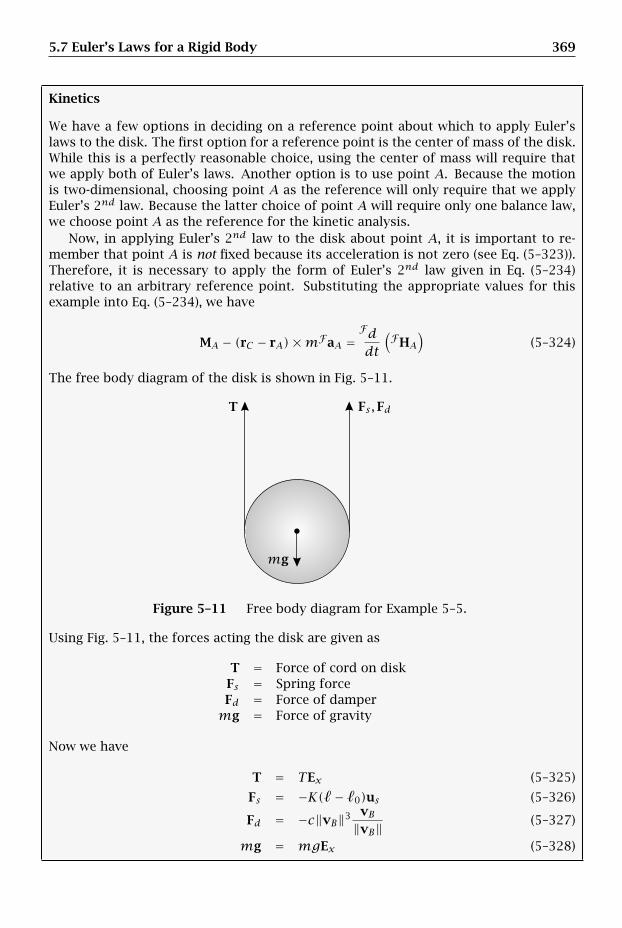
5.7 Euler’s Laws for a Rigid Body 369
Kinetics
We have a few options in deciding on a reference point about which to apply Euler’slaws to the disk. The first option for a reference point is the center of mass of the disk.While this is a perfectly reasonable choice, using the center of mass will require thatwe apply both of Euler’s laws. Another option is to use point A. Because the motionis two-dimensional, choosing point A as the reference will only require that we applyEuler’s 2nd law. Because the latter choice of point A will require only one balance law,we choose point A as the reference for the kinetic analysis.
Now, in applying Euler’s 2nd law to the disk about point A, it is important to re-member that point A is not fixed because its acceleration is not zero (see Eq. (5–323)).Therefore, it is necessary to apply the form of Euler’s 2nd law given in Eq. (5–234)relative to an arbitrary reference point. Substituting the appropriate values for thisexample into Eq. (5–234), we have
MA − (rC − rA)×mFaA =Fddt
(FHA
)(5–324)
The free body diagram of the disk is shown in Fig. 5–11.
Fs ,FdT
mg
Figure 5–11 Free body diagram for Example 5–5.
Using Fig. 5–11, the forces acting the disk are given as
T = Force of cord on diskFs = Spring forceFd = Force of dampermg = Force of gravity
Now we have
T = TEx (5–325)
Fs = −K( − 0)us (5–326)
Fd = −c‖vB‖3 vB‖vB‖
(5–327)
mg = mgEx (5–328)
370 Chapter 5. Kinetics of Rigid Bodies
Because the force T passes through point A, the moment applied to the disk relativeto point A is due entirely to the forces Fs , Fd, and mg, i.e.,
MA = (rs − rA)× Fs + (rd − rA)× Fd + (rg − rA)×mg (5–329)
where rs , rd, and rg are the positions at which the forces Fs , Fd, and mg act, respec-tively. From the geometry we have
rs = rBrd = rBrg = rC
(5–330)
Now, in order to obtain rB , we need to integrate FvB . First, recall FvB from Eq. (5–318)as
FvB = 2r θEx ≡FdrBdt
(5–331)
Separating variables in Eq. (5–331), we obtain
FdrB = 2r θExdt = 2rdθEx (5–332)
Integrating Eq. (5–332) gives
∫ rB
rB,0
FdrB =∫ θ
02rdνEx (5–333)
where rB,0 = rB(θ = 0) and ν is a dummy variable of integration. From Eq. (5–333), weobtain
rB − rB,0 = 2rθEx (5–334)
Because the disk rolls without slip, we have
rB,0 = −rEy (5–335)
Substituting rB,0 from Eq. (5–335) into (5–334), we obtain
rB + rEy = 2rθEx (5–336)
which implies thatrB = −rEy + 2rθEx (5–337)
Similarly, from Eq. (5–315) we have
FvC =Fddt(rC) = r θEx (5–338)
Separating variables, in Eq. (5–338), we obtain
FdrC = r θExdt = rdθEx (5–339)
Integrating Eq. (5–339) gives
∫ rC
rC,0
FdrC =∫ θ
0rdνEx (5–340)
5.7 Euler’s Laws for a Rigid Body 371
where rC,0 = rC(θ = 0) and ν is a dummy variable of integration. From Eq. (5–340), weobtain
rC − rC,0 = rθEx (5–341)
Now, because the disk rolls without slip, rC,0 = 0. Therefore,
rC = rθEx (5–342)
Consequently, the locations of the forces Fs , Fd, and mg are given, respectively, as
rs = 2rθEx − rEyrd = 2rθEx − rEyrg = rθEx
(5–343)
Next, from the geometry of the problem, the position of point A is given as
rA = rC + rEy = rθEx + rEy (5–344)
Subtracting rA in Eq. (5–344) from rs , rd, and rg , respectively, in Eq. (5–343), we obtain
rs − rA = rθEx − 2rEyrd − rA = rθEx − 2rEyrg − rA = −rEy
(5–345)
Now the position of point P is given in terms of the basis Ex,Ey,Ez as
rP = −LEx − rEy (5–346)
Substituting rB from Eq. (5–337) and rP from Eq. (5–346), we obtain
rB − rP = 2rθEx − rEy − (−LEx − rEy) = (2rθ + L)Ex (5–347)
The length of the spring is then given as
= ‖rB − rP‖ = ‖(2rθ + L)Ex‖ = 2rθ + L (5–348)
Furthermore, the unit vector in the direction along the spring is given as
us = rB − rP‖rB − rP‖
= (2rθ + L)Ex2rθ + L = Ex (5–349)
Then, substituting the results of Eqs. (5–348) and (5–349) into (5–326) and using thefact that 0 = L, we obtain the force in the linear spring as
Fs = −K [(2rθ + L)− L]Ex = −2KrθEx (5–350)
Furthermore, using the expression for FvB from Eq. (5–318), the force of the damperis obtained as
Fd = −c‖2r θEx‖3 2r θEx‖2r θEx‖
= −c(2r θ)3Ex
= −8cr 3θ3Ex
(5–351)
372 Chapter 5. Kinetics of Rigid Bodies
Then, using the values of rs − rA, rd − rA, and rg − rA from Eq. (5–345), the momentapplied about the point A is obtained as
MA = (rθEx − 2rEy)× [−2KrθEx]
+ (rθEx − 2rEy)×[−8cr 3θ3Ex
]− rEy ×mgEx
(5–352)
Noting that Ex × Ex = 0 and Ey × Ex = −Ez, Eq. (5–352) simplifies to
MA =[−4Kr 2θ − 16cr 4θ3 +mgr
]Ez (5–353)
Next, looking at Eq. (5–324), it is seen that it is necessary to compute the inertialmoment, i.e., we need to compute
−(rC − rA)×mFaA (5–354)
Substituting rC − rA and FaA from Eqs. (5–312) and (5–323), respectively, we have
−(rC − rA)×mFaA = −(−rEy)×m(−r θ2Ey) = 0 (5–355)
It is interesting to note that, although point A is not a fixed point, for this particularproblem, the inertial moment is zero. As a result, for the particular case of a uniformdisk rolling without slip along a flat surface, we can apply the fixed point form ofEuler’s 2nd law as given in Eq. (5–226).
Lastly, it is necessary to compute the rate of change of angular momentum of thedisk about point A. Using Eq. (5–24), we have the angular momentum about point A as
FHA = FHC + (rA − rC)×m(FvA − FvC) (5–356)
We have FHC asFHC = I
R · FωR = IRC · FωR (5–357)
Because Ex,Ey,Ez is a principal-axis basis, the moment of inertia tensor IRC is givenas
IRC = IxxEx ⊗ Ex + IyyEy ⊗ Ey + IzzEz ⊗ Ez (5–358)
Then, substituting IRC from Eq. (5–358) and FωR from Eq. (5–310), we obtain FHC as
FHC = IzzθEz (5–359)
Now we note that Izz is given as
Izz = mr2
2(5–360)
Consequently, we obtain FHC as
FHC = mr2
2θEz (5–361)
Then, using Eqs. (5–310), (5–313), and (5–315), and noting that FvA = 0, the secondterm of Eq. (5–356) is obtained as
(rA − rC)×m(FvA − FvC) = rEy ×m(−r θEx) =mr 2θEz (5–362)

5.7 Euler’s Laws for a Rigid Body 373
Adding the results of Eqs. (5–361) and (5–362), we obtain FHA as
FHA = mr2
2θEz +mr 2θEz = 3
2mr 2θEz (5–363)
Computing the rate of change of FHA in reference frame F , we obtain
Fddt
(FHA
)= 3
2mr 2θEz (5–364)
Then, because the inertial moment as given in Eq. (5–355) is zero, we can set MA from
Eq. (5–353) equal toFd(FHA)/dt from Eq. (5–364) to give
(−4Kr 2θEx − 16cr 4θ3 +mgr)Ez = 32mr
2θEz (5–365)
Rearranging Eq. (5–365) and dropping the dependence on Ez, we obtain the differentialequation of motion as
32mr
2θ + 16cr 4θ3 + 4Kr 2θ −mgr = 0 (5–366)
Example 5–6
A uniform sphere of massm and radius r rolls without slip along the surface of a fixedsphere, also of radius r , as shown in Fig. 5–12. The angle φ describes the rotation ofthe moving sphere from the vertical direction while the angle θ describes the locationof the center of mass of the sphere relative to the vertical. Knowing that gravity actsvertically downward, determine the differential equation of motion for the sphere interms of the angle θ.
No Slip
gm
r
rC
O
Pθ
φ
Figure 5–12 Sphere rolling on fixed spherical surface.
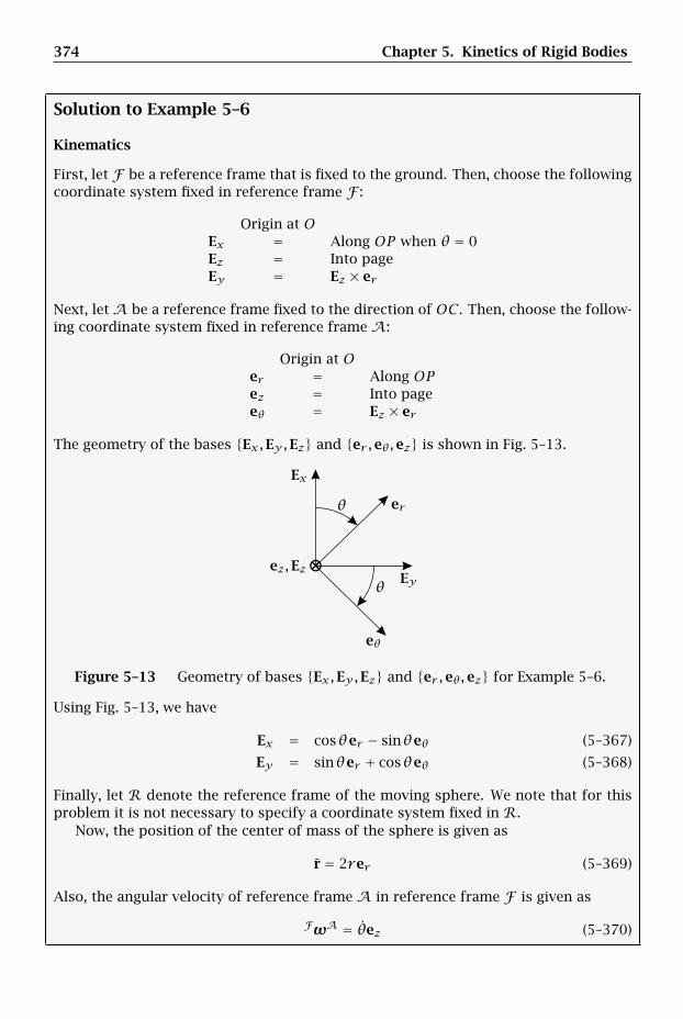
374 Chapter 5. Kinetics of Rigid Bodies
Solution to Example 5–6
Kinematics
First, let F be a reference frame that is fixed to the ground. Then, choose the followingcoordinate system fixed in reference frame F :
Origin at OEx = Along OP when θ = 0Ez = Into pageEy = Ez × er
Next, let A be a reference frame fixed to the direction of OC . Then, choose the follow-ing coordinate system fixed in reference frame A:
Origin at Oer = Along OPez = Into pageeθ = Ez × er
The geometry of the bases Ex,Ey,Ez and er ,eθ,ez is shown in Fig. 5–13.
⊗
er
eθ
Ex
Eyez,Ez
θ
θ
Figure 5–13 Geometry of bases Ex,Ey,Ez and er ,eθ,ez for Example 5–6.
Using Fig. 5–13, we have
Ex = cosθer − sinθeθ (5–367)
Ey = sinθer + cosθeθ (5–368)
Finally, let R denote the reference frame of the moving sphere. We note that for thisproblem it is not necessary to specify a coordinate system fixed in R.
Now, the position of the center of mass of the sphere is given as
r = 2rer (5–369)
Also, the angular velocity of reference frame A in reference frame F is given as
FωA = θez (5–370)
5.7 Euler’s Laws for a Rigid Body 375
Furthermore, because the angle φ is measured relative to the vertical direction, theangular velocity of reference frame R in reference frame F is given as
FωR = φez (5–371)
Applying the rate of change transport theorem of Eq. (2–128) on page 47 betweenreference frames A and F , the velocity of the center of mass of the sphere is
Fv =Fdrdt
=Adrdt+ FωA × r (5–372)
Now we have
Adrdt
= 0 (5–373)
FωA × r = θez × (2rer ) = 2r θeθ (5–374)
Adding Eqs. (5–373) and (5–374), we obtain
Fv = 2r θeθ (5–375)
Applying the rate of change transport theorem of Eq. (2–128) on page 47 to Fv betweenreference framesA and F , the acceleration of the center of mass of the sphere is givenas
Fa =Fddt
(Fv)=Addt
(Fv)+ FωA × Fv (5–376)
Now we have
Addt
(Fv)
= 2r θeθ (5–377)
FωA × Fv = θez × (2r θeθ) = −2r θ2er (5–378)
Adding Eqs. (5–377) and (5–378), we obtain the acceleration of the center of mass inreference frame F as
Fa = −2r θ2er + 2r θeθ (5–379)
A second expression for Fv is obtained as follows. Observing that points C and P arefixed in the sphere, from Eq. (2–517) we have
Fv = FvRP + FωR × (r− rP ) (5–380)
wherer− rP = rer (5–381)
Then, applying the rolling condition of Eq. (2–531) on page 109, we have
FvRP = 0 (5–382)
Consequently,Fv = φez × rer = rφeθ (5–383)
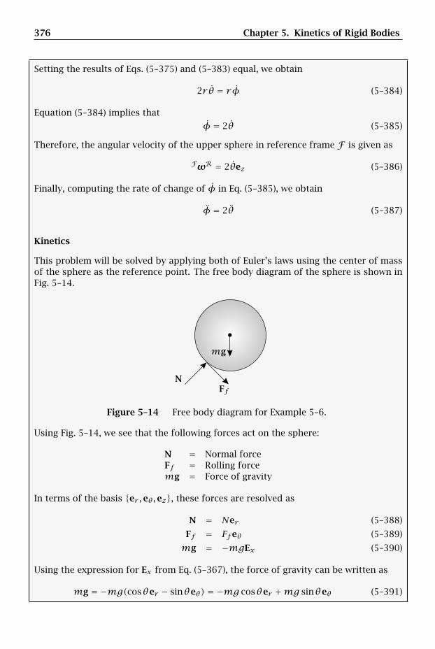
376 Chapter 5. Kinetics of Rigid Bodies
Setting the results of Eqs. (5–375) and (5–383) equal, we obtain
2r θ = rφ (5–384)
Equation (5–384) implies that
φ = 2θ (5–385)
Therefore, the angular velocity of the upper sphere in reference frame F is given as
FωR = 2θez (5–386)
Finally, computing the rate of change of φ in Eq. (5–385), we obtain
φ = 2θ (5–387)
Kinetics
This problem will be solved by applying both of Euler’s laws using the center of massof the sphere as the reference point. The free body diagram of the sphere is shown inFig. 5–14.
FfN
mg
Figure 5–14 Free body diagram for Example 5–6.
Using Fig. 5–14, we see that the following forces act on the sphere:
N = Normal forceFf = Rolling forcemg = Force of gravity
In terms of the basis er ,eθ,ez, these forces are resolved as
N = Ner (5–388)
Ff = Ffeθ (5–389)
mg = −mgEx (5–390)
Using the expression for Ex from Eq. (5–367), the force of gravity can be written as
mg = −mg(cosθer − sinθeθ) = −mg cosθer +mg sinθeθ (5–391)

5.7 Euler’s Laws for a Rigid Body 377
Application of Euler’s 1st Law to Center of Mass of Sphere
Using Eqs. (5–388), (5–389), and (5–391), the resultant force acting the sphere is givenas
F = Ner + Ffeθ −mg cosθer +mg sinθeθ= (N −mg cosθ)er + (Ff +mg sinθ)eθ
(5–392)
Applying Euler’s 1st law by setting F in Eq. (5–392) equal tomFa using Fa from Eq. (5–379), we obtain
(N −mg cosθ)er + (Ff +mg sinθ)eθ = −2mrθ2er + 2mrθeθ (5–393)
Equation (5–393) yields the following two scalar equations:
N −mg cosθ = −2mrθ2 (5–394)
Ff +mg sinθ = 2mrθ (5–395)
Application of Euler’s 2nd Law Relative to Center of Mass of Sphere
It is seen from Fig. 5–14 that the forces N and mg pass through the center of mass ofthe sphere while the force Ff acts at point P . Consequently, the moment applied tothe sphere relative to the center of mass of the sphere is given as
M = (rP − r)× Ff (5–396)
Now from Eq. (5–381) we haverP − r = −rer (5–397)
Therefore,M = −rer × Ffeθ = −rFfez (5–398)
Next, the angular momentum of the sphere relative to the center of mass of the sphereis given as
FH = I
R · FωR (5–399)
Then, since er ,eθ,ez is a principal-axis basis, the moment of inertia tensor IR
isgiven as
IR = Irrer ⊗ er + Iθθeθ ⊗ er + Izzez ⊗ ez (5–400)
Substituting IR
from Eq. (5–400) and FωR from Eq. (5–386), we obtain
FH = Izz2θez (5–401)
Using the fact that Izz = 2mr 2/5, we have
FH = 2
5mr 2(2θez) = 4
5mr 2θez (5–402)
Computing the rate of change ofF
H in reference frame F gives
Fddt
(FH)= 4
5mr 2θez (5–403)
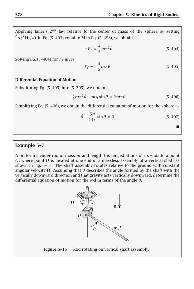
378 Chapter 5. Kinetics of Rigid Bodies
Applying Euler’s 2nd law relative to the center of mass of the sphere by settingFd(FH)/dt in Eq. (5–403) equal to M in Eq. (5–398), we obtain
−rFf =45mr 2θ (5–404)
Solving Eq. (5–404) for Ff gives
Ff = −45mrθ (5–405)
Differential Equation of Motion
Substituting Eq. (5–405) into (5–395), we obtain
−45mr
2θ +mg sinθ = 2mrθ (5–406)
Simplifying Eq. (5–406), we obtain the differential equation of motion for the sphere as
θ − 5g14r
sinθ = 0 (5–407)
Example 5–7
A uniform slender rod of mass m and length l is hinged at one of its ends to a pointO, where point O is located at one end of a massless assembly of a vertical shaft asshown in Fig. 5–15. The shaft assembly rotates relative to the ground with constantangular velocity Ω. Assuming that θ describes the angle formed by the shaft with thevertically downward direction and that gravity acts vertically downward, determine thedifferential equation of motion for the rod in terms of the angle θ.
g
m, l
O
θ
Ω
Figure 5–15 Rod rotating on vertical shaft assembly.
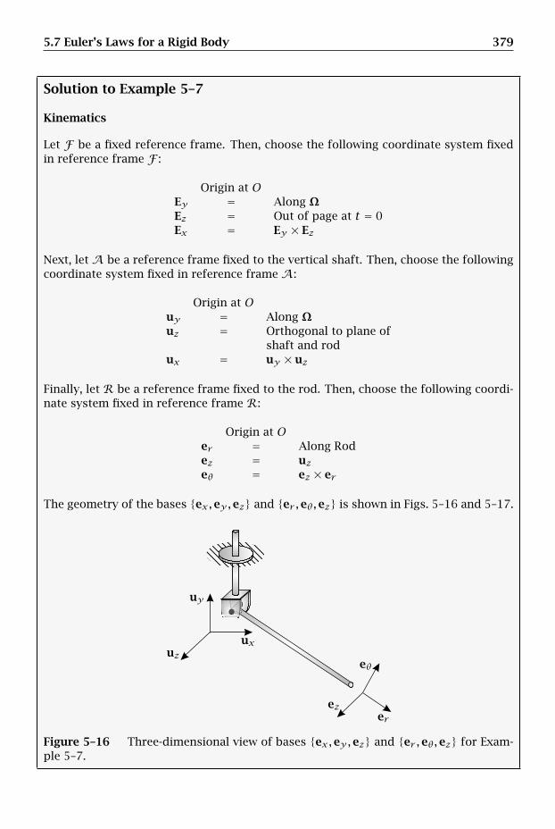
5.7 Euler’s Laws for a Rigid Body 379
Solution to Example 5–7
Kinematics
Let F be a fixed reference frame. Then, choose the following coordinate system fixedin reference frame F :
Origin at OEy = Along ΩEz = Out of page at t = 0Ex = Ey × Ez
Next, let A be a reference frame fixed to the vertical shaft. Then, choose the followingcoordinate system fixed in reference frame A:
Origin at Ouy = Along Ωuz = Orthogonal to plane of
shaft and rodux = uy × uz
Finally, let R be a reference frame fixed to the rod. Then, choose the following coordi-nate system fixed in reference frame R:
Origin at Oer = Along Rodez = uzeθ = ez × er
The geometry of the bases ex,ey,ez and er ,eθ,ez is shown in Figs. 5–16 and 5–17.
er
eθ
ez
ux
uy
uz
Figure 5–16 Three-dimensional view of bases ex,ey,ez and er ,eθ,ez for Exam-ple 5–7.
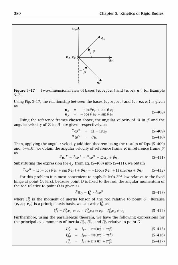
380 Chapter 5. Kinetics of Rigid Bodies
er
eθ
ux
uy
uz,ez
θ
θ
Figure 5–17 Two-dimensional view of bases ex,ey,ez and er ,eθ,ez for Example5–7.
Using Fig. 5–17, the relationship between the bases ex,ey,ez and er ,eθ,ez is givenas
ux = sinθer + cosθeθuy = − cosθer + sinθeθ
(5–408)
Using the reference frames chosen above, the angular velocity of A in F and theangular velocity of R in A, are given, respectively, as
FωA = Ω = Ωuy (5–409)AωR = θez (5–410)
Then, applying the angular velocity addition theorem using the results of Eqs. (5–409)and (5–410), we obtain the angular velocity of reference frame R in reference frame Fas
FωR = FωA +AωR = Ωuy + θez (5–411)
Substituting the expression for ey from Eq. (5–408) into (5–411), we obtain
FωR = Ω(− cosθer + sinθeθ)+ θez = −Ω cosθer +Ω sinθeθ + θez (5–412)
For this problem it is most convenient to apply Euler’s 2nd law relative to the fixedhinge at point O. First, because point O is fixed to the rod, the angular momentum ofthe rod relative to point O is given as
FHO = IRO · FωR (5–413)
where IRO is the moment of inertia tensor of the rod relative to point O. Becauseer ,eθ,ez is a principal-axis basis, we can write IRO as
IRO = IOrrer ⊗ er + IOθθeθ ⊗ eθ + IOzzez ⊗ ez (5–414)
Furthermore, using the parallel-axis theorem, we have the following expressions forthe principal-axis moments of inertia IOrr , I
Oθθ , and IOzz relative to point O:
IOrr = Irr +m(π2θ +π2
z ) (5–415)
IOθθ = Iθθ +m(π2r +π2
z ) (5–416)
IOzz = Izz +m(π2r +π2
θ) (5–417)
5.7 Euler’s Laws for a Rigid Body 381
where Irr , Iθθ , and Izz are the principal-axis moments of inertia of the rod relative tothe center of mass along the directions er , eθ , and ez, respectively, and πr , πθ , and πzare the distances in the er , eθ , and ez directions, respectively, by which the principal-axis system relative to the center of mass of the rod is translated to get to point O.Now we know for a uniform slender rod that
Irr = 0 (5–418)
Iθθ = ml2
12(5–419)
Izz = ml2
12(5–420)
Furthermore, in this case it is seen that only a translation along the er -direction by adistance l/2 is made in order to get from the center of mass to point O. Consequently,we have
πr = l2
(5–421)
πθ = 0 (5–422)
πz = 0 (5–423)
Substituting the results of Eqs. (5–418)–(5–420) and Eqs. (5–421)–(5–423) appropriatelyinto Eqs. (5–415)–(5–417), we obtain
IOrr = 0 (5–424)
IOθθ = ml2
12+m
(l2
)2
= ml2
3(5–425)
IOzz = ml2
12+m
(l2
)2
= ml2
3(5–426)
The moment of inertia tensor of Eq. (5–414) is then given as
IRO =ml2
3eθ ⊗ eθ + ml
2
3ez ⊗ ez (5–427)
Using the result of Eq. (5–427) together with the angular velocity FωR from Eq. (5–412),we obtain the angular momentum of the rod relative to point O as
FHO =(ml2
3eθ ⊗ eθ + ml
2
3ez ⊗ ez
)·(−Ω cosθer +Ω sinθeθ + θez
)(5–428)
Simplifying Eq. (5–428), we obtain
FHO = ml2
3Ω sinθeθ + ml
2
3θez (5–429)
Using the expression for FHO as given in Eq. (5–429), we need to obtain an expression
forFd(FHO)/dt. We have from the transport theorem that
Fddt
(FHO
)=Rddt
(FHO
)+ FωR × FHO (5–430)

382 Chapter 5. Kinetics of Rigid Bodies
where
Rddt
(FHO
)= ml2
3Ωθ cosθeθ + ml
2
3θez (5–431)
FωR × FHO =(−Ω cosθer +Ω sinθeθ + θez
)×(ml2
3Ω sinθeθ + ml
2
3θez
)
= −ml2
3Ω2 cosθ sinθez + ml
2
3Ω cosθθeθ
+ ml2
3Ωθ sinθer − ml
2
3Ωθ sinθer
= ml2
3Ωθ cosθeθ − ml
2
3Ω2 cosθ sinθez (5–432)
Then, adding Eqs. (5–431) and (5–432), we obtain
Fddt
(FHO
)= 2ml2
3Ωθ cosθeθ +
(ml2
3θ − ml
2
3Ω2 cosθ sinθ
)ez (5–433)
Kinetics
The free body diagram of the rod is shown in Fig. 5–18, from which it is seen that thefollowing forces act on the rod:
R = Reaction force of hinge on rodmg = Force of gravityτ = Pure torque due to prescribed rotation of shaft
It is emphasized that the pure torque applied by the shaft on the rod arises from thefact that the shaft is constrained to rotate with a known angular velocity. Furthermore,since this pure torque must be applied in the ey -direction (since the shaft rotates aboutthe ey -direction) and ey lies in the plane contained by er and eθ , the torque appliedby the shaft on the rod must have the form
τ = τr + τθ = τrer + τθeθ (5–434)
where τr and τθ are the components of the torque τ in the directions of er and eθ ,respectively.
R
mg
τr
τθ
Figure 5–18 Free body diagram of rod for Example 5–7.

5.7 Euler’s Laws for a Rigid Body 383
Now, from the geometry of the problem we have
R = Rrer + Rθeθmg = −mgey =mg cosθer −mg sinθeθτr = τrerτθ = τθeθ
(5–435)
Then, since R passes through point O, the moment due to all forces and torques rela-tive to point O is given as
MO = (r− rO)×mg+ τs + τr + τθ (5–436)
Now we note that
r− rO = l2er (5–437)
Consequently,
MO = l2er ×(−mg cosθer +mg sinθeθ
)+ τrer + τθeθ
= τrer + τθeθ + mgl2sinθez
(5–438)
Then, setting MO equal toFd(FHO)/dt using the expression for
Fd(FHO)/dt from
Eq. (5–433), we obtain
τrer + τθeθ + mgl2sinθez = 2ml2
3Ωθ cosθeθ
+(ml2
3θ − ml
2
3Ω2 cosθ sinθ
)ez
(5–439)
Simplifying Eq. (5–439), we obtain
mgl2
sinθez + τrer + τθeθ = 2ml2
3Ωθ cosθeθ
+(ml2
3θ − ml
2
3Ω2 cosθ sinθ
)ez
(5–440)
Equation (5–440) yields the following three scalar equations:
0 = τr (5–441)
2ml2
3Ωθ cosθ = τθ (5–442)
ml2
3θ − ml
2
3Ω2 cosθ sinθ = mgl
2sinθ (5–443)
It is interesting to note from Eq. (5–441) that the component of the pure torque dueto the shaft in the er -direction is zero. This result is absolutely consistent with thefact that the moment of inertia of the rod along the er -direction is zero, i.e., the shaftcannot exert a torque along a direction where the moment of inertia is zero. ExaminingEqs. (5–442) and (5–443), it is seen that Eq. (5–442) is indeterminate because τθ is
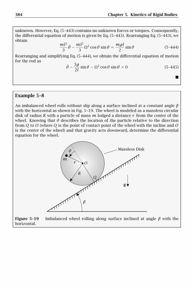
384 Chapter 5. Kinetics of Rigid Bodies
unknown. However, Eq. (5–443) contains no unknown forces or torques. Consequently,the differential equation of motion is given by Eq. (5–443). Rearranging Eq. (5–443), weobtain
ml2
3θ − ml
2
3Ω2 cosθ sinθ = mgl
2sinθ (5–444)
Rearranging and simplifying Eq. (5–444), we obtain the differential equation of motionfor the rod as
θ − 3g2l
sinθ −Ω2 cosθ sinθ = 0 (5–445)
Example 5–8
An imbalanced wheel rolls without slip along a surface inclined at a constant angle βwith the horizontal as shown in Fig. 5–19. The wheel is modeled as a massless circulardisk of radius R with a particle of mass m lodged a distance r from the center of thewheel. Knowing that θ describes the location of the particle relative to the directionfrom Q to O (where Q is the point of contact point of the wheel with the incline and Ois the center of the wheel) and that gravity acts downward, determine the differentialequation for the wheel.
Massless Disk
g
mr O
QR
β
θ
Figure 5–19 Imbalanced wheel rolling along surface inclined at angle β with thehorizontal.
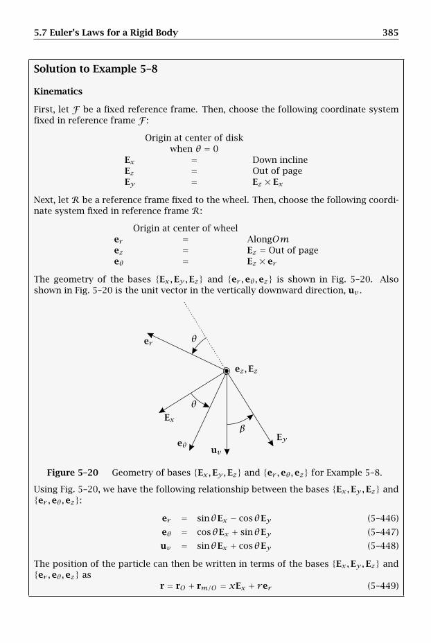
5.7 Euler’s Laws for a Rigid Body 385
Solution to Example 5–8
Kinematics
First, let F be a fixed reference frame. Then, choose the following coordinate systemfixed in reference frame F :
Origin at center of diskwhen θ = 0
Ex = Down inclineEz = Out of pageEy = Ez × Ex
Next, let R be a reference frame fixed to the wheel. Then, choose the following coordi-nate system fixed in reference frame R:
Origin at center of wheeler = AlongOmez = Ez = Out of pageeθ = Ez × er
The geometry of the bases Ex,Ey,Ez and er ,eθ,ez is shown in Fig. 5–20. Alsoshown in Fig. 5–20 is the unit vector in the vertically downward direction, uv .
er
eθ
Ex
Ey
ez,Ez
uv
β
θ
θ
Figure 5–20 Geometry of bases Ex,Ey,Ez and er ,eθ,ez for Example 5–8.
Using Fig. 5–20, we have the following relationship between the bases Ex,Ey,Ez ander ,eθ,ez:
er = sinθEx − cosθEy (5–446)
eθ = cosθEx + sinθEy (5–447)
uv = sinθEx + cosθEy (5–448)
The position of the particle can then be written in terms of the bases Ex,Ey,Ez ander ,eθ,ez as
r = rO + rm/O = xEx + rer (5–449)
386 Chapter 5. Kinetics of Rigid Bodies
where
rO = xEx (5–450)
rm/O = rer (5–451)
We have from Eq. (5–450) thatFvO = xEx (5–452)
Now, because the wheel rolls without slip along a fixed surface, we have
FvQ = 0 (5–453)
Furthermore, because θ is measured from a direction fixed in the inertial referenceframe F , the angular velocity of the wheel in reference frame F is given as
FωR = θez = θEz (5–454)
Then, applying Eq. (2–517) on page 106, the velocity of point O in reference frame Fis obtained as
FvO = FvQ + FωR × (rO − rQ) = FωR × (rO − rQ) (5–455)
Now we haverO − rQ = −REy (5–456)
Substituting the expressions for FωR and rO − rQ from Eqs. (5–454) and (5–456, re-spectively, we have
FvO = θEz × (−rEy) = RθEx (5–457)
Setting the expressions for FvO in Eqs. (5–452) and (5–457), we obtain
x = Rθ (5–458)
Integrating Eq. (5–458) using the fact that θ(t = 0) = 0, we obtain
x = Rθ (5–459)
The position of the particle can then be written in terms of the angle θ as
r = RθEx + rer (5–460)
Computing the rate of change of r in reference frame F , the velocity of the particle inreference frame F is given as
Fv =Fdrdt
=Fddt(rO)+
Fddt
(rm/O
) = FvO + Fvm/O (5–461)
Because the basis Ex,Ey,Ez is fixed in reference frame F , we have
FvO =FdrOdt
= r θEx (5–462)
Furthermore, because rm/O is expressed in the basis er ,eθ,ez, we obtain
Fvm/O =Fddt
(rm/O
) = Rddt
(rm/O
)+ FωR × rm/O (5–463)
5.7 Euler’s Laws for a Rigid Body 387
Now we haveRddt
(rm/O
) = 0 (5–464)
FωR × rm/O = θez × rer = r θeθ (5–465)
Adding the expressions in Eqs. (5–464) and (5–465), we obtain
Fvm/O = r θeθ (5–466)
Then, adding Eqs. (5–462) and (5–466), the velocity of the particle in reference frameF is given as
Fv = RθEx + r θeθ (5–467)
Next, the acceleration of the particle in reference frame F is given from the transporttheorem of Eq. (2–128) on page 47 as
Fa =Fddt
(Fv)=Fddt
(FvO
)+Fddt
(Fvm/O
)= FaO + Fam/O (5–468)
First, we have
FaO =Fddt
(FvO
)= RθEx (5–469)
Next, applying the rate of change transport theorem to Fvm/O between referenceframes R and F , we obtain Fam/O as
Fam/O =Fddt
(Fvm/O
)=Rddt
(Fvm/O
)+ FωR × Fvm/O (5–470)
Now the two terms on the right-hand side of Eq. (5–470) are given as
Rddt
(Fvm/O
)= r θeθ (5–471)
FωR × Fvm/O = θez × r θeθ = −r θ2er (5–472)
Adding the expressions in Eqs. (5–471) and (5–472), we obtain
Fam/O = −r θ2er + r θeθ (5–473)
Then, adding Eqs. (5–469) and (5–473), we obtain the acceleration of the particle inreference frame F as
Fa = RθEx − r θ2er + r θeθ (5–474)
Kinetics
Because the wheel rolls without slip, it is convenient to use the point of contact, Q, asthe reference point. Now, as discussed in Section 2.15.4 of Chapter 2, while the velocityof the point of contact in reference frame F is zero, i.e., FvQ = 0, the acceleration ofthe point of contact in reference frame F is not zero. Therefore, we must apply thegeneral form of Euler’s 2nd law when using the contact point as the reference, i.e.,
MQ − (r− rQ)×mFaQ =Fddt
(FHQ
)(5–475)
The free body diagram of the wheel is shown in Fig. 5–21.
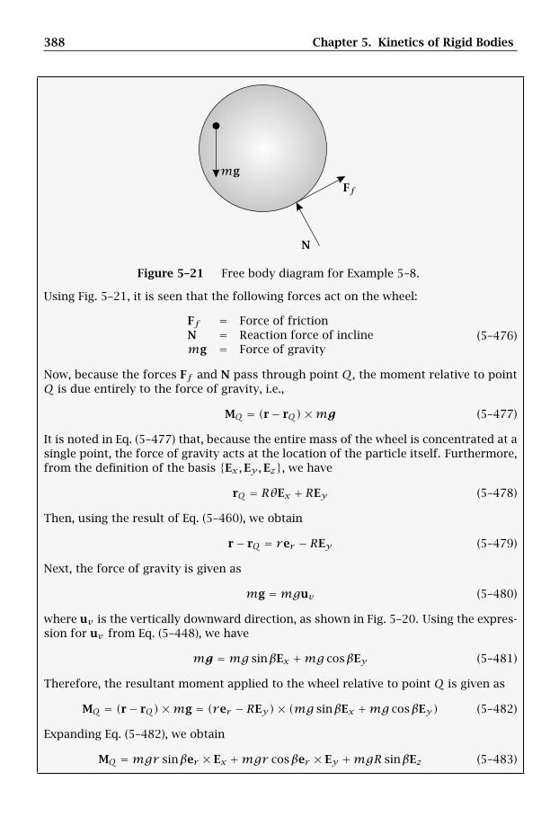
388 Chapter 5. Kinetics of Rigid Bodies
Ff
N
mg
Figure 5–21 Free body diagram for Example 5–8.
Using Fig. 5–21, it is seen that the following forces act on the wheel:
Ff = Force of frictionN = Reaction force of inclinemg = Force of gravity
(5–476)
Now, because the forces Ff and N pass through point Q, the moment relative to pointQ is due entirely to the force of gravity, i.e.,
MQ = (r− rQ)×mg (5–477)
It is noted in Eq. (5–477) that, because the entire mass of the wheel is concentrated at asingle point, the force of gravity acts at the location of the particle itself. Furthermore,from the definition of the basis Ex,Ey,Ez, we have
rQ = RθEx + REy (5–478)
Then, using the result of Eq. (5–460), we obtain
r− rQ = rer − REy (5–479)
Next, the force of gravity is given as
mg =mguv (5–480)
where uv is the vertically downward direction, as shown in Fig. 5–20. Using the expres-sion for uv from Eq. (5–448), we have
mg =mg sinβEx +mg cosβEy (5–481)
Therefore, the resultant moment applied to the wheel relative to point Q is given as
MQ = (r− rQ)×mg = (rer − REy)× (mg sinβEx +mg cosβEy) (5–482)
Expanding Eq. (5–482), we obtain
MQ =mgr sinβer × Ex +mgr cosβer × Ey +mgR sinβEz (5–483)
5.7 Euler’s Laws for a Rigid Body 389
Using the expression for er in Eq. (5–446), we have
er × Ex = (sinθEx − cosθEy)× Ex = cosθEz = cosθez (5–484)
er × Ey = (sinθEx − cosθEy)× Ey = sinθEz = sinθez (5–485)
Substituting the results of Eqs. (5–484) and (5–485), respectively, into Eq. (5–483), wehave
MQ =mgr sinβ cosθez +mgr cosβ sinθez +mgR sinβEz (5–486)
Simplifying Eq. (5–486) and noting that Ez = ez, we obtain
MQ =mg [r(sinβ cosθ + cosβ sinθ)+ R sinβ]ez (5–487)
Now from trigonometry we have
sinβ cosθ + cosβ sinθ = sin(θ + β) (5–488)
Consequently, the moment applied to the disk relative to point Q is given as
MQ =mg [r sin(θ + β)+ R sinβ]ez (5–489)
Next, the acceleration of the point of contact is given as
FaQ = aO + FαR × (rQ − rO)+ FωR ×[FωR × (rQ − rO)
](5–490)
where we note that
FαR =Fddt
(FωR
)= θez = θEz (5–491)
Also, noting that rQ − rO = REy , we obtain
FaQ = RθEx + θEz × (REy)+ θEz ×[θEz × (REy)
]= −Rθ2Ey (5–492)
Therefore, the inertial moment is given as
−(r− rQ)×mFaQ = −(r− rQ)×mFaQ = −(rer − REy)×m(−Rθ2Ey)
=mRrθ2er × Ey =mRrθ2 sinθez(5–493)
It is noted in Eq. (5–493) that we have used the expression for er ×Ey from Eq. (5–485)and have also used the fact that the mass of the system is concentrated at a singlepoint.
Next, the angular momentum of the disk relative to point Q in reference frame Fcan be obtained from Eq. (5–24) as
FHQ = FH+ (rQ − r)×m(FvQ − Fv) (5–494)
Because the mass is concentrated at a single point, the angular momentum relative tothe center of mass of the system is zero, i.e.,
FH = 0 (5–495)
390 Chapter 5. Kinetics of Rigid Bodies
Consequently, we obtain FHQ as
FHQ = (rQ − r)×m(FvQ − Fv) (5–496)
Furthermore, observing that r = r and Fv = Fv, where r is the position of the particleand Fv = Fv is the velocity of the particle in reference frame F , Eq. (5–496) can bewritten as
FHQ = (rQ − r)×m(FvQ − Fv) (5–497)
Computing the rate of change of FHQ from Eq. (5–497) in reference frame F , we obtain
Fddt
(FHQ
)= (rQ − r)×m(FaQ − Fa) (5–498)
Then, using r − rQ, Fa, and FaQ from Eqs. (5–479), (5–474), and (5–492), respectively,
we obtainFd(FHQ
)/dt as
Fddt
(FHQ
)= (−rer + REy)×m
[−Rθ2Ey − (RθEx − r θ2er + r θeθ)
]= (−rer + REy)×m(−Rθ2Ey − RθEx + r θ2er − r θeθ)
(5–499)
Expanding Eq. (5–499) gives
Fddt
(FHQ
)=mRrθ2er × Ey +mRrθer × Ex +mr 2θEz
+mR2θEz +mRrθ2Ey × er −mRrθEy × eθ
(5–500)
Now we already have expressions for er×Ex and er×Ey from Eqs. (5–484) and (5–485),respectively. In addition, we have
Ey × eθ = Ey × (cosθEx + sinθEy) = − cosθEz (5–501)
Substituting the results of Eqs. (5–484), (5–485), and (5–501) into Eq. (5–500), we obtain
Fddt
(FHQ
)=mRrθ2 sinθEz +mRrθ cosθEz +mr 2θEz
+mR2θEz −mRrθ2 sinθEz +mRrθ cosθEz
(5–502)
Equation (5–502) simplifies to
Fddt
(FHQ
)=m(r 2 + R2 + 2rR cosθ)θEz =m(r 2 + R2 + 2rR cosθ)θez (5–503)
Finally, substituting MQ, −(r − rQ) ×mFaQ, andFd(FHQ
)/dt from Eq. (5–489), (5–
493), and (5–503), respectively, into (5–475) we obtain
mg [r sin(θ + β)+ R sinβ]ez +mRrθ2 sinθez =m(r 2+R2+2rR cosθ)θez (5–504)
Rearranging and dropping the common component of ez, we obtain the differentialequation of motion as
m(r 2 + R2 + 2rR cosθ)θ −mrRθ2 sinθ −mgr sin(θ + β)−mgR sinβ = 0 (5–505)
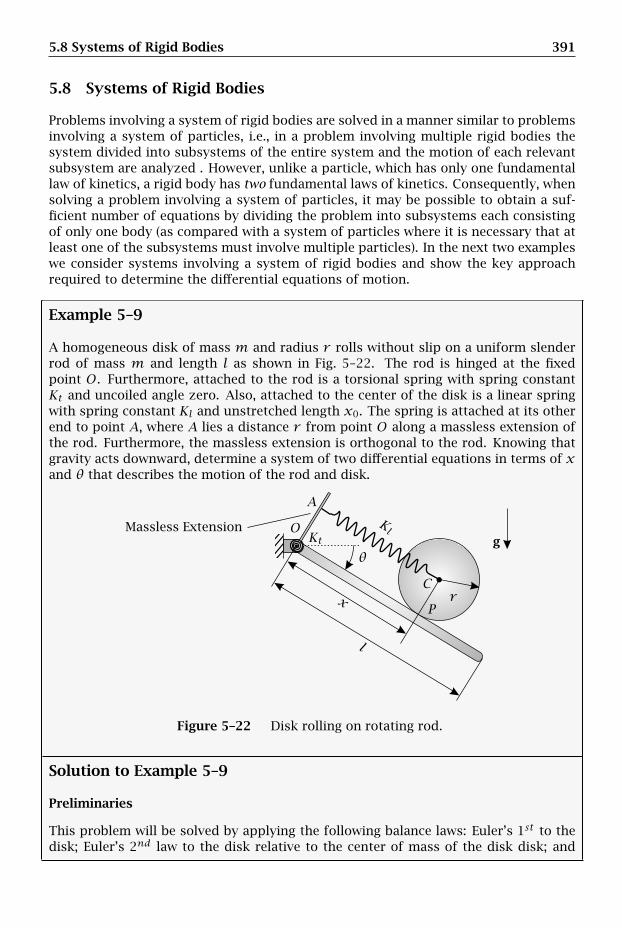
5.8 Systems of Rigid Bodies 391
5.8 Systems of Rigid Bodies
Problems involving a system of rigid bodies are solved in a manner similar to problemsinvolving a system of particles, i.e., in a problem involving multiple rigid bodies thesystem divided into subsystems of the entire system and the motion of each relevantsubsystem are analyzed . However, unlike a particle, which has only one fundamentallaw of kinetics, a rigid body has two fundamental laws of kinetics. Consequently, whensolving a problem involving a system of particles, it may be possible to obtain a suf-ficient number of equations by dividing the problem into subsystems each consistingof only one body (as compared with a system of particles where it is necessary that atleast one of the subsystems must involve multiple particles). In the next two exampleswe consider systems involving a system of rigid bodies and show the key approachrequired to determine the differential equations of motion.
Example 5–9
A homogeneous disk of mass m and radius r rolls without slip on a uniform slenderrod of mass m and length l as shown in Fig. 5–22. The rod is hinged at the fixedpoint O. Furthermore, attached to the rod is a torsional spring with spring constantKt and uncoiled angle zero. Also, attached to the center of the disk is a linear springwith spring constant Kl and unstretched length x0. The spring is attached at its otherend to point A, where A lies a distance r from point O along a massless extension ofthe rod. Furthermore, the massless extension is orthogonal to the rod. Knowing thatgravity acts downward, determine a system of two differential equations in terms of xand θ that describes the motion of the rod and disk.
Massless Extensiong
l
Kl
Kt
rx
A
C
O
P
θ
Figure 5–22 Disk rolling on rotating rod.
Solution to Example 5–9
Preliminaries
This problem will be solved by applying the following balance laws: Euler’s 1st to thedisk; Euler’s 2nd law to the disk relative to the center of mass of the disk disk; and
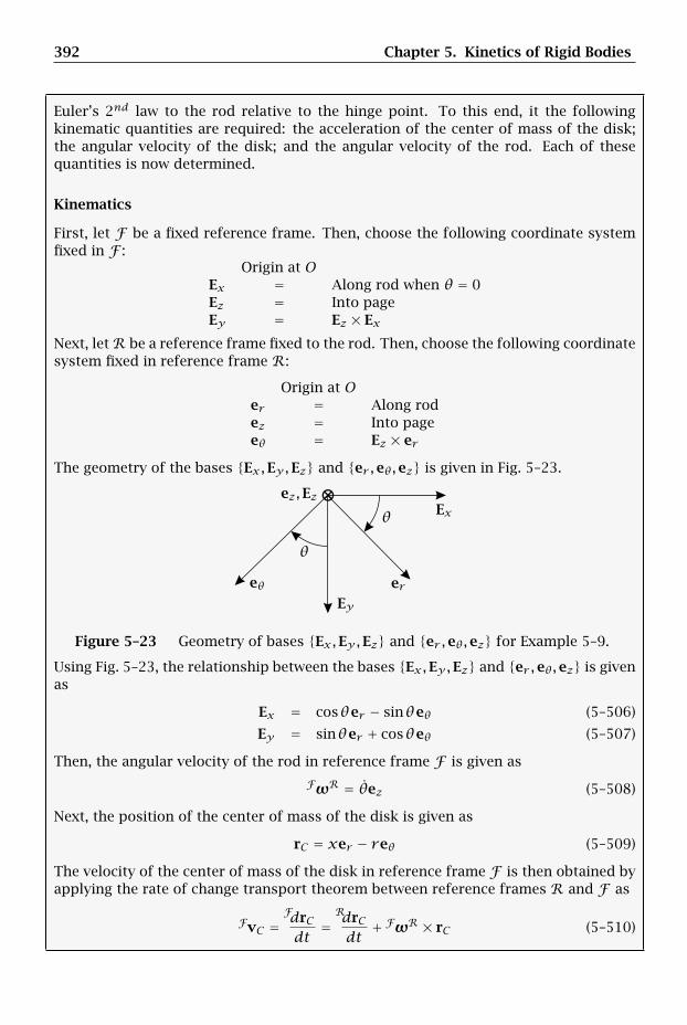
392 Chapter 5. Kinetics of Rigid Bodies
Euler’s 2nd law to the rod relative to the hinge point. To this end, it the followingkinematic quantities are required: the acceleration of the center of mass of the disk;the angular velocity of the disk; and the angular velocity of the rod. Each of thesequantities is now determined.
Kinematics
First, let F be a fixed reference frame. Then, choose the following coordinate systemfixed in F :
Origin at OEx = Along rod when θ = 0Ez = Into pageEy = Ez × Ex
Next, letR be a reference frame fixed to the rod. Then, choose the following coordinatesystem fixed in reference frame R:
Origin at Oer = Along rodez = Into pageeθ = Ez × er
The geometry of the bases Ex,Ey,Ez and er ,eθ,ez is given in Fig. 5–23.
⊗
ereθ
Ex
Ey
ez,Ezθ
θ
Figure 5–23 Geometry of bases Ex,Ey,Ez and er ,eθ,ez for Example 5–9.
Using Fig. 5–23, the relationship between the bases Ex,Ey,Ez and er ,eθ,ez is givenas
Ex = cosθer − sinθeθ (5–506)
Ey = sinθer + cosθeθ (5–507)
Then, the angular velocity of the rod in reference frame F is given as
FωR = θez (5–508)
Next, the position of the center of mass of the disk is given as
rC = xer − reθ (5–509)
The velocity of the center of mass of the disk in reference frame F is then obtained byapplying the rate of change transport theorem between reference frames R and F as
FvC =FdrCdt
=RdrCdt
+ FωR × rC (5–510)
5.8 Systems of Rigid Bodies 393
Now we have
RdrCdt
= xer (5–511)
FωR × rC = θez × (xer − reθ) = r θer + xθeθ (5–512)
Adding Eqs. (5–511) and (5–512), the velocity of the center of mass of the disk inreference frame F is obtained as
FvC = (x + r θ)er + xθeθ (5–513)
Next, the acceleration of the center of mass of the disk in reference frameF is obtainedby applying the rate of change transport theorem between reference frames R and Fto FvC as
FaC =Fddt
(FvC
)=R ddt
(FvC
)+ FωR × FvC (5–514)
Now we have
R ddt
(FvC
)= (x + r θ)er + (xθ + xθ)eθ (5–515)
FωR × FvC = θez ×[(x + r θ)er + xθeθ
]= −xθ2er + θ(x + r θ)eθ (5–516)
Adding Eqs. (5–515) and (5–516) gives
FaC = (x + r θ)er + (xθ + xθ)eθ − xθ2er + θ(x + r θ)eθ (5–517)
Simplifying Eq. (5–517), we obtain the acceleration of the center of mass of the disk inreference frame F as
FaC = (x + r θ − xθ2)er + (2xθ + xθ + r θ2)eθ (5–518)
Next, we need to determine the angular velocity of the disk in reference frame F .Suppose we denote the reference frame of the disk by D. Then, since the motion isplanar, we have
FωD =ωez (5–519)
Furthermore, considering point P to be fixed to the disk, we have from Eq. (2–517) onpage 106 that
FvC = FvP + FωD × (rC − rP ) (5–520)
Furthermore, from the geometry we have
rC = xer − reθ (5–521)
rP = xer (5–522)
Therefore,rC − rP = xer − reθ − xer = −reθ (5–523)
Substituting FωD and rC − rP from Eqs. (5–519) and (5–523), respectively, into Eq. (5–520), we obtain
FvC = FvP +ωez × (−reθ) = FvP + rωer (5–524)
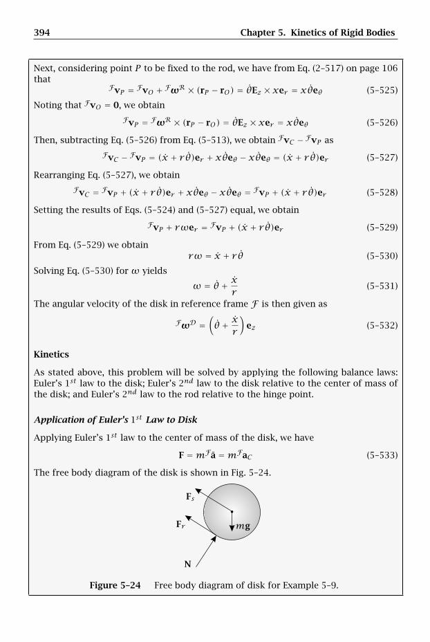
394 Chapter 5. Kinetics of Rigid Bodies
Next, considering point P to be fixed to the rod, we have from Eq. (2–517) on page 106that
FvP = FvO + FωR × (rP − rO) = θEz × xer = xθeθ (5–525)
Noting that FvO = 0, we obtain
FvP = FωR × (rP − rO) = θEz × xer = xθeθ (5–526)
Then, subtracting Eq. (5–526) from Eq. (5–513), we obtain FvC − FvP as
FvC − FvP = (x + r θ)er + xθeθ − xθeθ = (x + r θ)er (5–527)
Rearranging Eq. (5–527), we obtain
FvC = FvP + (x + r θ)er + xθeθ − xθeθ = FvP + (x + r θ)er (5–528)
Setting the results of Eqs. (5–524) and (5–527) equal, we obtain
FvP + rωer = FvP + (x + r θ)er (5–529)
From Eq. (5–529) we obtainrω = x + r θ (5–530)
Solving Eq. (5–530) for ω yields
ω = θ + xr
(5–531)
The angular velocity of the disk in reference frame F is then given as
FωD =(θ + x
r
)ez (5–532)
Kinetics
As stated above, this problem will be solved by applying the following balance laws:Euler’s 1st law to the disk; Euler’s 2nd law to the disk relative to the center of mass ofthe disk; and Euler’s 2nd law to the rod relative to the hinge point.
Application of Euler’s 1st Law to Disk
Applying Euler’s 1st law to the center of mass of the disk, we have
F =mFa =mFaC (5–533)
The free body diagram of the disk is shown in Fig. 5–24.
Fr
Fs
N
mg
Figure 5–24 Free body diagram of disk for Example 5–9.
5.8 Systems of Rigid Bodies 395
Using Fig. 5–24, we have
FR = Rolling force of rod on diskN = Normal force of rod on diskmg = Force of gravityFs = Force of linear spring
Now from the geometry we have
FR = FReθ (5–534)
N = Neθ (5–535)
mg = mgEy =mg sinθer +mg cosθeθ (5–536)
Fs = −Kl(x − x0)er (5–537)
where we have used in Eq. (5–536) the expression for Ey from Eq. (5–507). Conse-quently,
F = FRer +Neθ +mg sinθer +mg cosθeθ −Kl(x − x0)er= [FR +mg sinθ −Kl(x − x0)
]er +
[mg cosθ +N]eθ
(5–538)
Then, setting F equal tomFaC using the expression for FaC from Eq. (5–518), we obtain[FR +mg sinθ −Kl(x − x0)
]er +
[mg cosθ +N]eθ
=m(x + r θ − xθ2)er+m(2xθ + xθ + r θ2)eθ
(5–539)
Equating components, we obtain the following two scalar equations:
FR +mg sinθ −Kl(x − x0) = m(x + r θ − xθ2) (5–540)
mg cosθ +N = m(2xθ + xθ + r θ2) (5–541)
Application of Euler’s 2nd Law to Disk Relative to Center of Mass of Disk
Applying Euler’s law relative to the center of mass of the disk, we have
MC =Fddt
(FHC
)(5–542)
Again it is seen from Fig. 5–24 that the forces mg, Fs , and N pass through point C .Consequently, the moment relative to the center of mass of the disk is given as
MC = (rP − rC)× FR (5–543)
Using the fact that rP − rC = reθ , we have
MC = reθ × FRer = −rFREz (5–544)
Now the angular momentum of the disk relative to its center of mass is given as
FHC = ID · FωD (5–545)
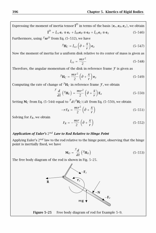
396 Chapter 5. Kinetics of Rigid Bodies
Expressing the moment of inertia tensor ID
in terms of the basis er ,eθ,ez, we obtain
ID = Irrer ⊗ er + Iθθeθ ⊗ eθ + Izzez ⊗ ez (5–546)
Furthermore, using FωD from Eq. (5–532), we have
FHC = Izz(θ + x
r
)ez (5–547)
Now the moment of inertia for a uniform disk relative to its center of mass is given as
Izz = mr2
2(5–548)
Therefore, the angular momentum of the disk in reference frame F is given as
FHC = mr2
2
(θ + x
r
)ez (5–549)
Computing the rate of change of FHC in reference frame F , we obtain
F ddt
(FHC
)= mr
2
2
(θ + x
r
)Ez (5–550)
Setting MC from Eq. (5–544) equal toFd(FHC)/dt from Eq. (5–550), we obtain
−rFR = mr2
2
(θ + x
r
)(5–551)
Solving for FR, we obtain
FR = −mr2(θ + x
r
)(5–552)
Application of Euler’s 2nd Law to Rod Relative to Hinge Point
Applying Euler’s 2nd law to the rod relative to the hinge point, observing that the hingepoint is inertially fixed, we have
MO =Fddt
(FHO
)(5–553)
The free body diagram of the rod is shown in Fig. 5–25.
−Fr
−Fs
−N
R
mg
τs
Figure 5–25 Free body diagram of rod for Example 5–9.
5.8 Systems of Rigid Bodies 397
Using Fig. 5–25, we have
R = Reaction force of hinge on rod−N = Reaction force of disk on rod−FR = Rolling force of disk on rodmg = Force of gravity−Fs = Force of linear springτs = Pure torque due to torsional spring
First, the reaction force of the hinge on the rod is given in terms of the basis er ,eθ,ezas
R = Rrer + Rθeθ (5–554)
Furthermore, using the expressions for FR, N, mg, and Fs from Eqs. (5–534)–(5–537)we have, respectively,
−N = −Neθ (5–555)
−FR = −FRer (5–556)
mg = mgEy =mg sinθer + cosθeθ (5–557)
−Fs = Kl(x − x0)er (5–558)
where in Eq. (5–557) we have used the expression for Ey from Eq. (5–507). Finally, thepure torque due to the torsional spring is given as
τs = −Kτθez (5–559)
The moment applied to the rod relative to point O is then given as
MO = rO × R+ (r− rO)×mg+ (rP − rO)× (−N− FR)+ (rA − rO)× (−Fs)+ τs
(5–560)
Observing that r−rO = (l/2)er , rA−rO = −reθ , and rP−rO = xer , Eq. (5–560) becomes
MO = l2er ×
[mg sinθer +mg cosθeθ
]+ xer × (−Neθ − FRer )+ (−reθ)× (Kl(x − x0)er )−Kτθez
=(mgl
2cosθ − xN + rKl(x − x0)−Kτθ
)ez
(5–561)
Next, the angular momentum of the rod relative to point O in reference frame F isgiven as
FHO = IR · FωR (5–562)
Now since er ,eθ,ez is a principle-axis basis for the rod, we have
IR = IOrrer ⊗ er + IOθθeθ ⊗ eθ + IOzzez ⊗ ez (5–563)
Then, using the expression for FωR from Eq. (5–508), we obtain FHO as
FHO = (IOrrer ⊗ er + IOθθeθ ⊗ eθ + IOzzez ⊗ ez) · θez = IOzzθEz (5–564)
398 Chapter 5. Kinetics of Rigid Bodies
Now for a slender uniform rod we have
Izz = ml2
12(5–565)
Then, applying the parallel-axis theorem, we obtain
IOzz = Izz +m(π2r +π2
θ) (5–566)
Now since in this case the translation is performed in only the er -direction, we have
πr = l2
(5–567)
πθ = 0 (5–568)
Therefore,
IO = ml2
12+m
(l2
)2
= ml2
3(5–569)
The angular momentum of the rod relative to the hinge point in reference frame F isthen given as
FHO = ml2
3θez (5–570)
Computing the rate of change of FHO in reference frame F , we obtain which impliesthat
Fddt
(FHO
)= ml
2
3θez (5–571)
Setting MO from Eq. (5–561) equal toFd(FHO)/dt from Eq. (5–571), we obtain
mgl2
cosθ − xN + rKl(x − x0)−Kτθ = ml2
3θ (5–572)
System of Two Differential Equations
We can now use the results of parts (b), (c), and (d) to obtain a system of two differentialequations that describes the motion of the rod and the disk. First, substituting theexpression for FR from Eq. (5–552) into Eq. (5–540), we obtain
−mr2
(θ + x
r
)+mg sinθ −Kl(x − x0) =m(x + r θ − xθ2) (5–573)
Rearranging Eq. (5–573), we have
m(x + r θ − xθ2)+ mr2
(θ + x
r
)+Kl(x − x0)−mg sinθ = 0 (5–574)
Simplifying Eq. (5–574), we obtain the first differential equation as
32mx + 3
2mrθ −mxθ2 +Kl(x − x0)−mg sinθ = 0 (5–575)
Next, solving Eq. (5–541) for N, we obtain
N =m(2xθ + xθ + r θ2)−mg cosθ (5–576)

5.8 Systems of Rigid Bodies 399
Substituting the expression for N from Eq. (5–576) into Eq. (5–572), we have
mgl2
cosθ − x[m(2xθ + xθ + r θ2)+mg cosθ
]
+ rKl(x − x0)−Kτθ = ml2
3θ
(5–577)
Rearranging Eq. (5–577), we obtain the second differential equation as
m(l2
3+ x2
)θ+2mxxθ+mrxθ2+mg
(x − l
2
)cosθ−rKl(x−x0)+Kτθ = 0 (5–578)
The system of two differential equations for the rod and the disk is then given as
32mx + 3
2mrθ −mxθ2 +Kl(x − x0)−mg sinθ = 0 (5–579)
m(l2
3+ x2
)θ+2mxxθ+mrxθ2+mg
(x − l
2
)cosθ−rKl(x−x0)+Kτθ = 0 (5–580)
Example 5–10
A system consists of two barrels that roll without slip in the vertical plane as shownin Fig. 5–26. The barrels are modeled as thin cylindrical shells of mass m and radiusr . The lower barrel rolls without slip along a fixed horizontal surface while the upperbarrel rolls without slip along the lower barrel. Knowing that gravity acts downward,determine a system of two differential equations in terms of the angles θ and φ thatdescribes the motion of the barrels.
No Slip
g
m
m
r
rC
O
P
Q
θ
φ
Figure 5–26 Two barrels rolling along one another.
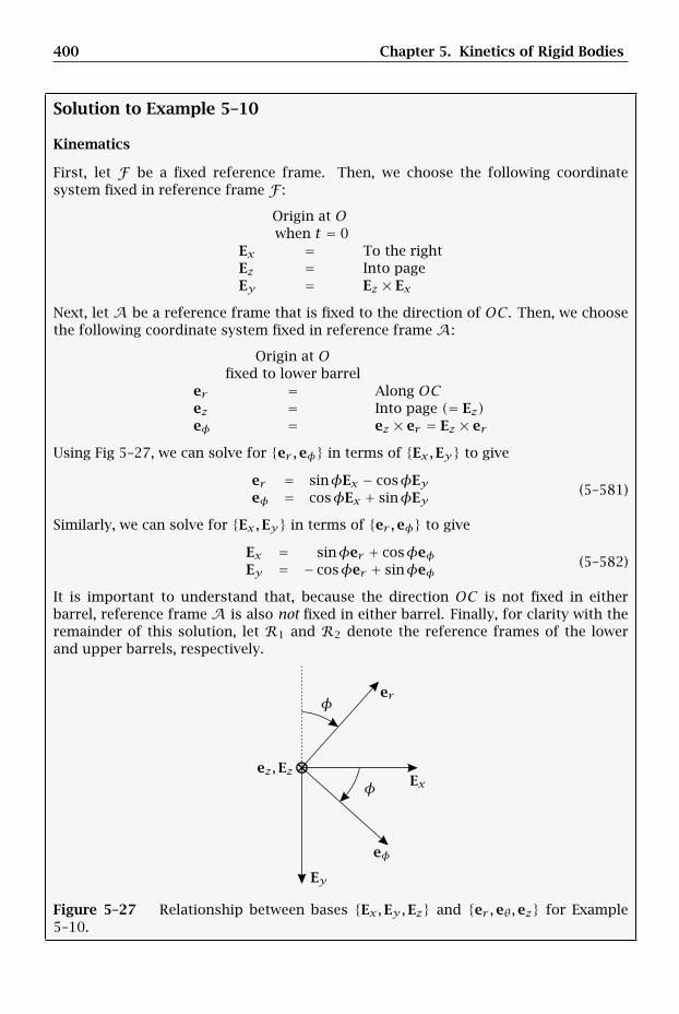
400 Chapter 5. Kinetics of Rigid Bodies
Solution to Example 5–10
Kinematics
First, let F be a fixed reference frame. Then, we choose the following coordinatesystem fixed in reference frame F :
Origin at Owhen t = 0
Ex = To the rightEz = Into pageEy = Ez × Ex
Next, let A be a reference frame that is fixed to the direction of OC . Then, we choosethe following coordinate system fixed in reference frame A:
Origin at Ofixed to lower barrel
er = Along OCez = Into page (= Ez)eφ = ez × er = Ez × er
Using Fig 5–27, we can solve for er ,eφ in terms of Ex,Ey to give
er = sinφEx − cosφEyeφ = cosφEx + sinφEy
(5–581)
Similarly, we can solve for Ex,Ey in terms of er ,eφ to give
Ex = sinφer + cosφeφEy = − cosφer + sinφeφ
(5–582)
It is important to understand that, because the direction OC is not fixed in eitherbarrel, reference frame A is also not fixed in either barrel. Finally, for clarity with theremainder of this solution, let R1 and R2 denote the reference frames of the lowerand upper barrels, respectively.
⊗
er
eφ
Ex
Ey
ez,Ezφ
φ
Figure 5–27 Relationship between bases Ex,Ey,Ez and er ,eθ,ez for Example5–10.
5.8 Systems of Rigid Bodies 401
Now, looking ahead to the kinetics of this problem, it is clear that we will needto apply some form of Euler’s laws to the system and/or subsystems of the system.Consequently, it is necessary to determine those kinematic quantities that are requiredto apply Euler’s laws. In particular, in this problem the following kinematic quantitiesare relevant and must be computed in reference frame F : the angular velocity of thelower barrel; the velocity and acceleration of the center of mass of the lower barrel;the angular velocity of the upper barrel; and the velocity and acceleration of the centerof mass of the upper barrel. Each of these quantities will now be computed.
Angular Velocity of Lower Barrel
Because the angle θ describes the absolute rotation of the lower barrel relative toreference frame F , the angular velocity of the lower barrel in reference frame F isgiven as
FωR1 = θEz (5–583)
Velocity and Acceleration of Center of Mass of Lower Barrel
We note that Q is the instantaneous point of contact of the lower barrel with theground. Because the lower barrel rolls without slip on the ground and the ground is afixed surface, we have
FvQ = 0 (5–584)
Also, applying Eq. (2–517) on page 106, we have
FvO − FvQ = FωR1 × (rO − rQ) (5–585)
In addition, from the geometry we have
rO − rQ = −rEy (5–586)
Using FωR1 from Eq. (5–583) and the fact that FvQ = 0, we obtain
FvO = θEz × (−rEy) = r θEx (5–587)
Computing the rate of change of FvO in reference frame F , we have
FaO =Fddt
(FvO
)= r θEx (5–588)
Angular Velocity of Upper Barrel
First, from the geometry of the problem we have
rC − rO = 2rer (5–589)
Computing the rate of change of rC − rO in reference frame F , we obtain
FvC − FvO =Fddt(rC − rO) = 2rφeφ (5–590)
402 Chapter 5. Kinetics of Rigid Bodies
Equation (5–590) implies that
FvC = FvO + 2rφeφ (5–591)
Substituting the result for FvO from Eq. (5–587), we obtain
FvC = r θEx + 2rφeφ (5–592)
We can obtain a second expression for FvC as follows. Noting that P is the point ofcontact between the lower and upper barrels and that the upper barrel rolls withoutslip on the lower barrel, we know from Eq. (2–525) that the velocity of point P inreference frame F is the same on either barrel, i.e.,
FvR1P = FvR2
P ≡ FvP (5–593)
Then, because we are considering point P to be fixed to the lower barrel, we have
FvP − FvO = FωR1 × (rP − rO) (5–594)
From the geometry we haverP − rO = rer (5–595)
Then, substituting rP−rO from Eq. (5–595) and FωR1 from Eq. (5–583) into Eq. (5–594),we obtain
FvP − FvO = θEz × rer = r θeφ (5–596)
Equation (5–594) implies that
FvP = FvO + r θeφ = r θEx + r θeφ (5–597)
Next, because this time we are considering point P to be fixed to the upper barrel, wehave
FvC − FvP = FωR2 × (rC − rB) (5–598)
where FωR2 is the angular velocity of the upper barrel in reference frame F . Becausethe motion is planar, we can write FωR2 as
FωR2 =ω2Ez (5–599)
Furthermore, from the geometry we have
rC − rB = rer (5–600)
Therefore, we obtainFvC − FvP =ω2Ez × rer = rω2eφ (5–601)
Solving for FvC , we obtainFvC = FvP + rω2eφ (5–602)
Substituting the result for FvP from Eq. (5–597), we obtain a second expression forFvC as
FvC = r θEx + r θeφ + rω2eφ = r θEx + r(θ +ω2)eφ (5–603)
5.8 Systems of Rigid Bodies 403
Then, setting the expressions for FvC from Eqs. (5–592) and (5–603) equal, we obtain
r θEx + 2rφeφ = r θEx + r(θ +ω2)eφ (5–604)
Simplifying Eq. (5–604), we obtain
2rφeφ = r(θ +ω2)eφ (5–605)
Then, from Eq. (5–605) we have
2rφ = r(θ +ω2) (5–606)
Solving Eq. (5–606) for ω2, we obtain
ω2 = 2φ− θ (5–607)
The angular velocity of the upper barrel in reference frame F is then given as
FωR2 = (2φ− θ)Ez (5–608)
Acceleration of Center of Mass of Upper Barrel
Computing the rate of change of FvC as given in Eq. (5–592) in reference frame F , theacceleration of the center of mass of the upper barrel is given as
FaC =Fddt
(FvC
)= r θEx − 2rφ2er + 2rφeφ (5–609)
Kinetics
For this problem we will apply the following balance laws: (1) Euler’s 2nd law relativeto the contact point of the lower barrel with the ground, (2) Euler’s 1st law to the upperbarrel, and (3) Euler’s 2nd law relative to the center of mass of the upper barrel.
Application of Euler’s 2nd Law to Lower Barrel Relative to Instantaneous Point ofContact with Ground
The free body diagram of the lower barrel is shown in Fig. 5–28. Using Fig. 5–28, wehave
N1 = Reaction force of ground on lower barrelR1 = Rolling force of ground on lower barrelmg = Force of gravityN2 = Reaction force of upper barrel on lower barrelR2 = Rolling force of upper barrel on lower barrel
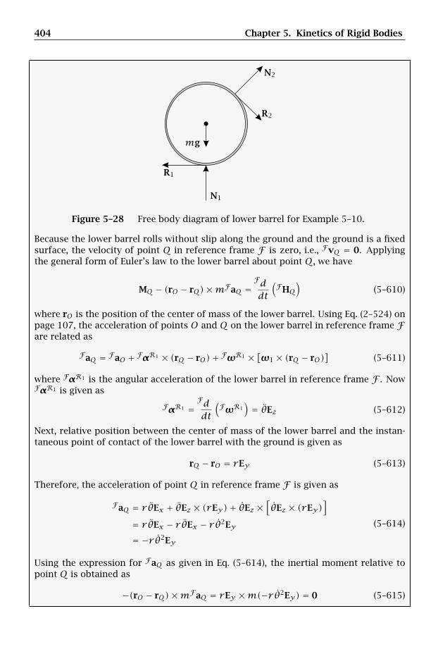
404 Chapter 5. Kinetics of Rigid Bodies
N1
N2
R1
R2
mg
Figure 5–28 Free body diagram of lower barrel for Example 5–10.
Because the lower barrel rolls without slip along the ground and the ground is a fixedsurface, the velocity of point Q in reference frame F is zero, i.e., FvQ = 0. Applyingthe general form of Euler’s law to the lower barrel about point Q, we have
MQ − (rO − rQ)×mFaQ =Fddt
(FHQ
)(5–610)
where rO is the position of the center of mass of the lower barrel. Using Eq. (2–524) onpage 107, the acceleration of points O and Q on the lower barrel in reference frame Fare related as
FaQ = FaO + FαR1 × (rQ − rO)+ FωR1 × [ω1 × (rQ − rO)]
(5–611)
where FαR1 is the angular acceleration of the lower barrel in reference frame F . NowFαR1 is given as
FαR1 =Fddt
(FωR1
)= θEz (5–612)
Next, relative position between the center of mass of the lower barrel and the instan-taneous point of contact of the lower barrel with the ground is given as
rQ − rO = rEy (5–613)
Therefore, the acceleration of point Q in reference frame F is given as
FaQ = r θEx + θEz × (rEy)+ θEz ×[θEz × (rEy)
]= r θEx − r θEx − r θ2Ey
= −r θ2Ey
(5–614)
Using the expression for FaQ as given in Eq. (5–614), the inertial moment relative topoint Q is obtained as
−(rO − rQ)×mFaQ = rEy ×m(−r θ2Ey) = 0 (5–615)
5.8 Systems of Rigid Bodies 405
We see that, because the lower barrel is modeled as a homogeneous thin cylindricalshell, the inertial moment of the lower barrel relative to the instantaneous point ofcontact is zero. Using the result from Eq. (5–615), for this problem we have
MQ =Fddt
(FHQ
)(5–616)
Next, examining Fig. 5–28, we see that the forces N1, R1, and mg all pass throughpoint Q. Therefore, the moment about point Q is due entirely to the forces N2 and R2
and is given asMQ = (rP − rQ)× (N2 + R2) (5–617)
where we note that both N2 and R2 act at the instantaneous point of contact of thelower barrel with the upper barrel (i.e., point P ). Now, because N2 and R2 are thereaction force and rolling force, respectively, applied by the upper barrel to the lowerbarrel, we have
N2 = N2erR2 = R2eφ
(5–618)
Furthermore, we haverP − rQ = rer − rEy (5–619)
The moment applied to the lower barrel relative to point Q is then given as
MQ = (rer − rEy)× (N2er + R2eφ) (5–620)
Expanding Eq. (5–620), we obtain
MQ = −rN2Ey × er + rR2er × eφ − rR2Ey × eφ (5–621)
Computing the relevant vector products in Eq. (5–621), we have
er × eφ = EzEy × er = Ey × (sinφEx − cosφEy) = − sinφEzEy × eφ = Ey × (cosφEx + sinφEy) = − cosφEz
(5–622)
Substituting the expressions from Eq. (5–622) into (5–621), we obtain
MQ = rN2 sinφEz + rR2Ez + rR2 cosφEz (5–623)
Factoring out Ez from the last expression, we obtain the moment applied to the lowerbarrel relative to the instantaneous point of contact Q as
MQ = [rN2 sinφ+ rR2(1+ cosφ)]Ez (5–624)
Finally, we need to compute the rate of change of the angular momentum of the lowerbarrel relative to point Q in reference frame F . First, the angular momentum relativeto the center of mass of the lower barrel in reference frame F is given as
FHO = IR1O · FωR1 (5–625)
406 Chapter 5. Kinetics of Rigid Bodies
where we note that point O is the center of mass of the lower barrel. Now, becauseEx,Ey,Ez is a principal-axis basis, the moment of inertia relative to the center ofmass of the lower barrel is given as
IR1 = IOxxEx ⊗ Ex + IOyyEy ⊗ Ey + IOzzEz ⊗ Ez (5–626)
Then, using FωR1 from Eq. (5–583), we have
FHO = (IOxxEx ⊗ Ex + IOyyEy ⊗ Ey + IOzzEz ⊗ Ez) · θEz = IOzzθEz (5–627)
Next, using Eq. (5–24), the angular momentum of the lower barrel in reference frameF relative to point Q is given as
FHQ = FHO + (rQ − rO)×m(FvQ − FvO) (5–628)
Using the fact that FvQ = 0, we have from Eq. (5–587) that
FvQ − FvO = −FvO = −r θEx (5–629)
Furthermore, substituting Eqs. (5–613), (5–627), and (5–629) into Eq. (5–628), we obtain
FHQ = IzzθEz + (rEy)×m(−r θEx) = IzzθEz +mr 2θEz = (Izz +mr 2)θEz (5–630)
Because the barrel is modeled as a thin cylindrical shell, we have
IOzz =mr 2 (5–631)
Consequently, FHQ simplifies to
FHQ = 2mr 2θEz (5–632)
Computing the rate of change of FHQ in reference frame F , we obtain
Fddt
(FHQ
)= 2mr 2θEz (5–633)
Then, substituting MQ andFd(FHQ)/dt from Eqs. (5–624) and (5–632), respectively,
into (5–616), we have
rN2 sinφ+ rR2(1+ cosφ) = 2mr 2θ (5–634)
Simplifying this last expression by dividing through by r , we obtain the scalar equation
2mrθ = N2 sinφ+ R2(1+ cosφ) (5–635)
Application of Euler’s 1st Law to Upper Barrel
The free body diagram of the upper barrel is shown in Fig. 5–29, where
mg = Force of gravity−N2 = Reaction force of lower barrel on upper barrel−R2 = Rolling force of lower barrel on upper barrel
We note that, from Newton’s 3rd law, the forces applied by the lower barrel on theupper barrel are equal and opposite to the forces applied by the upper barrel on thelower barrel (see Fig. 5–28).

5.8 Systems of Rigid Bodies 407
−R2
−N2
mg
Figure 5–29 Free body diagram of upper barrel for Example 5–10.
Applying Euler’s 1st law to the center of mass of the upper barrel, we have
F2 =mFaC (5–636)
where F2 is the resultant force on the upper barrel. From the free body diagram ofFig. 5–29 we have that
F2 =mg−N2 − R2 (5–637)
Substituting the expressions for N2 and R2 from Eq. (5–618), we obtain
F2 =mgEy −N2er − R2eφ (5–638)
Now we can substitute the expression for Ey in terms of er and eφ from Eq. (5–582)into the last equation. This gives
F2 =mg(− cosφer + sinφeφ)−N2er − R2eφ (5–639)
Simplifying this last expression gives
F2 = −(N2 +mg cosφ)er + (mg sinφ− R2)eφ (5–640)
Then, using the result for the acceleration of the center of mass of the upper barrelfrom Eq. (5–609), we can equate F2 and mFaC to obtain
−(N2 +mg cosφ)er + (mg sinφ− R2)eφ =mrθEx − 2mrφ2er + 2mrφeφ (5–641)
Then, in order to get an equation in terms of a single coordinate system, we can substi-tute the expression for Ex in terms of er and eφ from Eq. (5–582) into the last equation.This gives
−(N2 +mg cosφ)er + (mg sinφ− R2)eφ =mrθ(sinφer + cosφeφ)
− 2mrφ2er + 2mrφeφ(5–642)
Simplifying Eq. (5–642), we obtain
−(N2 +mg cosφ)er + (mg sinφ− R2)eφ = mr(θ sinφ− 2φ2)er+mr(θ cosφ+ 2φ)eφ
(5–643)
Equating components in Eq. (5–643) yields the following two scalar equations:
−N2 −mg cosφ = mrθ sinφ− 2mrφ2 (5–644)
mg sinφ− R2 = mrθ cosφ+ 2mrφ (5–645)
408 Chapter 5. Kinetics of Rigid Bodies
Application of Euler’s 2nd Law to Upper Barrel Relative to Center of Mass of UpperBarrel
Applying Euler’s 2nd law to the upper barrel using the center of mass of the upperbarrel as the reference point, we have
MC =Fddt
(FHC
)(5–646)
Examining the free body diagram of the upper barrel as shown in Fig. 5–29, we seethat the force of gravity mg and the reaction force −N2 both pass through point C .Consequently, the moment about point C is due to only the force −R2 and is given as
MC = (rR2 − rC)× (−R2) (5–647)
Now, from the geometry we have
rR2 − rC = −rer (5–648)
Therefore,MC = −rer × (−R2eφ) = rR2Ez (5–649)
Now we need the rate of change of angular momentum of the upper barrel about pointC . First, we have
FHC = IR2C · FωR2 (5–650)
Furthermore, the moment of inertia tensor relative to point C for the upper barrel isgiven in terms of the basis Ex,Ey,Ez as
IR2C = ICxxEx ⊗ Ex + ICyyEy ⊗ Ey + ICzzEz ⊗ Ez (5–651)
Then, using FωR2 from Eq. (5–608), we obtain the angular momentum of the upperbarrel relative to point C as
FHC = (ICxxEx ⊗ Ex + ICyyEy ⊗ Ey + ICzzEz ⊗ Ez) · FωR2 = ICzz(2φ− θ)Ez (5–652)
Because the upper barrel is modeled as a thin cylindrical shell and Ex,Ey,Ez is aprincipal-axis basis relative to the center of mass of the upper barrel, we have
ICzz =mr 2 (5–653)
Consequently, we obtain FHC as
FHC =mr 2(2φ− θ)Ez (5–654)
Computing the rate of change of FHC in reference frame F gives
Fddt
(FHC
)=mr 2(2φ− θ)Ez (5–655)
Setting MC from Eq. (5–649) equal toFd(FHC)/dt from Eq. (5–655) gives
rR2Ez =mr 2(2φ− θ)Ez (5–656)
Dropping the dependence on Ez and simplifying, we obtain the scalar equation
R2 =mr(2φ− θ) (5–657)

5.8 Systems of Rigid Bodies 409
System of Two Differential Equations
We can now use Eqs. (5–635), (5–644), (5–645), and (5–657) to obtain a system of twodifferential equations. The first differential equation is obtained by substituting R2
from Eq. (5–657) into (5–645). This gives
mg sinφ−mr(2φ− θ) =mrθ cosφ+ 2mrφ (5–658)
Rearranging and simplifying Eq. (5–658), we obtain the first differential equation as
r θ(1+ cosφ)+ 4rφ− g sinφ = 0 (5–659)
The second differential equation is obtained as follows. Multiplying Eqs. (5–644) and(5–645) by sinφ and cosφ, respectively, we obtain
−N2 sinφ−mg cosφ sinφ = mrθ sin2φ− 2mrφ2 sinφ (5–660)
mg sinφ cosφ− R2 cosφ = mrθ cos2φ+ 2mrφ cosφ (5–661)
Adding Eqs. (5–660) and (5–661) gives
−N2 sinφ− R2 cosφ =mrθ(sin2φ+ cos2φ)− 2mrφ2 sinφ+ 2mrφ cosφ (5–662)
Noting that sin2φ+ cos2φ ≡ 1, we have
−N2 sinφ− R2 cosφ =mrθ − 2mrφ2 sinφ+ 2mrφ cosφ (5–663)
Next, augmenting the result of Eq. (5–635) to (5–663), we obtain the following twoequations:
−N2 sinφ− R2 cosφ = mrθ − 2mrφ2 sinφ+ 2mrφ cosφ (5–664)
N2 sinφ+ R2(1+ cosφ) = 2mrθ (5–665)
Adding Eqs. (5–664) and (5–665), we have
R2 = 3mrθ + 2mrφ cosφ− 2mrφ2 sinφ (5–666)
Substituting the expression for R2 from Eq. (5–657) into (5–665) gives
mr(2φ− θ) = 3mrθ + 2mrφ cosφ− 2mrφ2 sinφ (5–667)
Rearranging and simplifying Eq. (5–667), we obtain the second differential equation ofmotion as
2θ − (1− cosφ)φ− φ2 sinφ = 0 (5–668)
The system of two differential equations without reaction forces is then given as
(2 cosφ− 1) r θ + 6rφ− 2g sinφ = 0 (5–669)
2θ − (1− cosφ)φ− φ2 sinφ = 0 (5–670)
410 Chapter 5. Kinetics of Rigid Bodies
5.9 Rotational Dynamics of a Rigid Body Using Moment of Inertia
Because the angular momentum of a rigid body is conveniently represented in termsof the moment of inertia tensor, it is useful to derive a special set of results for the ro-tational dynamics of a rigid body in terms of the moment of inertia. It is also useful tounderstand the stability of motion of a rigid body when it rotates about a direction thatis in the neighborhood of a principal axis. In this section we derive the coordinate-freeresults for the rotational motion of a rigid body. Subsequently, we derive a special setof results in terms of a body-fixed coordinate system. Then, the body-fixed rotationalequations are specialized further to the case of a principal-axis body-fixed coordinatesystem. These latter results are referred to as Euler’s equations. Finally, using Euler’sequations, the stability of the rotational motion in the neighborhood of a principal-axisis analyzed.
5.9.1 Euler’s 2nd Law in Terms of Moment of Inertia Tensor
Recall that the angular momentum of a rigid body R relative to a point Q fixed in Rcan be written in terms of the moment of inertia tensor IRQ as
NHQ = IRQ · NωR (5–671)
Computing the rate of change of NHQ in Eq. (5–671) in an inertial reference frame N ,we have
Nddt
(NHQ
)=Nddt
(IRQ · NωR
)(5–672)
Then, applying the rate of change transport theorem of Eq. (2–128) on page 47, weobtain
Nddt
(IRQ · NωR
)=Rddt
(IRQ · NωR
)+NωR ×
(IRQ · NωR
)(5–673)
Furthermore, we have
Rddt
(IRQ · NωR
)=Rddt
(IRQ)· NωR + IRQ ·
Rddt
(NωR
)(5–674)
Using the result of Eq. (5–674), we have
Nddt
(NHQ
)=Rddt
(IRQ)· NωR + IRQ ·
Rddt
(NωR
)+NωR ×
(IRQ · NωR
)(5–675)
Now we note thatNddt
(NωR
)= NαR
which then becomes
Nddt
(NHQ
)=Rddt
(IRQ)· NωR + IRQ · NαR +NωR ×
(IRQ · NωR
)(5–676)
We then have
MQ − (r− rQ)×mNaQ =Rddt
(IRQ)· NωR + IRQ · NαR +NωR ×
(IRQ · NωR
)(5–677)
5.9 Rotational Dynamics of a Rigid Body Using Moment of Inertia 411
Now we recall that the moment of inertia tensor IRQ can be expressed in terms of abody-fixed coordinate system as
IRQ =3∑i=1
3∑j=1
IQijei ⊗ ej (5–678)
Then, because e1,e2,e3 is a body-fixed basis, we have
Rdeidt
= 0 , (i = 1,2,3) (5–679)
Furthermore, recall from Eqs. (5–54) and (5–55) that the moments and products ofinertia IQij (i, j = 1,2,3) in terms of a body-fixed coordinate system are constant. Con-
sequently, the rate of change of IRQ as viewed by an observer in the rigid body is zero,i.e.,
Rddt
(IRQ)= O (5–680)
where O is the zero tensor. Applying the result of Eq. (5–680) in (5–677), we have
MQ − (r− rQ)×mNaQ = IRQ · NαR +NωR ×(IRQ · NωR
)(5–681)
We note in Eq. (5–681) that
Nddt
(NHQ
)= IRQ · NαR +NωR ×
(IRQ · NωR
)(5–682)
Equation (5–677) is a coordinate-free form of Euler’s 2nd law in terms of the momentof inertia tensor relative to a point Q fixed in the rigid body.
Suppose now that we choose the reference point to be the center of mass of therigid body. Then r− rQ = r− r = 0 and Eq. (5–681) simplifies to
M = IR · NαR +NωR ×
(IR · NωR
)(5–683)
where, in a manner similar to Eq. (5–681), we note that
Nddt
(NH)= I
R · NαR +NωR ×(IR · NωR
)(5–684)
Equation (5–683) is a coordinate-free form of Euler’s 2nd law in terms of the momentof inertia tensor relative to the center of mass of the rigid body.
5.9.2 Euler’s Equations for a Rigid Body
While Eq. (5–683) provides a coordinate-free way to describe the rotational motionof a rigid body relative to the center of mass of the body, it is often convenient towrite Eq. (5–683) in terms of a specific body-fixed coordinate system. To this end, lete1,e2,e3 be a body-fixed basis. Then in terms of e1,e2,e3 we can write
NωR =ω1e1 +ω2e2 +ω3e3 (5–685)
412 Chapter 5. Kinetics of Rigid Bodies
Computing the rate of change of NωR in reference frame N (and recalling that therate of change of NωR is the same in references frames N and R), we obtain
Nddt
(NωR
)=Nddt
(NωR
)= ω1e1 + ω2e2 + ω3e3 (5–686)
Furthermore, the moment of inertia tensor can be written in the body-fixed basise1,e2,e3 as
IR = I11e1 ⊗ e1 + I12e1 ⊗ e2 + I12e1 ⊗ e3
+ I12e2 ⊗ e1 + I22e2 ⊗ e2 + I13e2 ⊗ e3
+ I13e3 ⊗ e1 + I23e3 ⊗ e2 + I33e3 ⊗ e3
(5–687)
Using Eqs. (5–685), (5–686), and (5–687), we obtain
IR · NωR = (I11ω1 + I12ω2 + I13ω3)e1
+ (I12ω1 + I22ω2 + I23ω3)e2
+ (I13ω1 + I23ω2 + I33ω3)e3
(5–688)
and
IR · NαR = (I11ω1 + I12ω2 + I13ω3)e1
+ (I12ω1 + I22ω2 + I23ω3)e2
+ (I13ω1 + I23ω2 + I33ω3)e3
(5–689)
Suppose now that we let
H1 = (I11ω1 + I12ω2 + I13ω3) (5–690)
H2 = (I12ω1 + I22ω2 + I23ω3) (5–691)
H3 = (I13ω1 + I23ω2 + I33ω3) (5–692)
Then,
NωR ×(IR · NωR
)= (H3ω2 −H2ω3)e1 + (H1ω3 −H3ω1)e2
+ (H2ω1 −H1ω2)e3
(5–693)
Also, letM = M1e1 + M2e2 + M3e3 (5–694)
Substituting the results of Eqs. (5–689), (5–693), and (5–694) into Eq. (5–683), we obtainthe following three scalar equations:
M1 = I11ω1 + I12ω2 + I13ω3 +H3ω2 −H2ω3 (5–695)
M2 = I12ω1 + I22ω2 + I23ω3 +H1ω3 −H3ω1 (5–696)
M3 = I13ω1 + I23ω2 + I33ω3 +H2ω1 −H1ω2 (5–697)
5.9 Rotational Dynamics of a Rigid Body Using Moment of Inertia 413
Finally, substituting the expressions in Eqs. (5–690)–(5–692) into Eqs. (5–695)–(5–697),respectively, we have
M1 = I11ω1 + I12(ω2 −ω1ω3)+ I13(ω3 +ω1ω2)+(I33 − I22)ω3ω2 + I23(ω2
2 −ω23) (5–698)
M2 = I12(ω1 +ω2ω3)+ I22ω2 + I23(ω3 −ω1ω2)+(I11 − I33)ω1ω3 + I13(ω2
3 −ω21) (5–699)
M3 = I13(ω1 −ω2ω3)+ I23(ω2 +ω1ω3)+ I33ω3
+(I22 − I11)ω2ω1 + I12(ω21 −ω2
2) (5–700)
It can be seen that Eqs. (5–698)–(5–700) are quite complicated since they involve all ofthe moments and products of inertia. Suppose now that e1,e2,e3 is a principal-axisbasis. Then Eqs. (5–698)–(5–700) simplify to
M1 = I1ω1 + (I3 − I2)ω3ω2 (5–701)
M2 = I2ω2 + (I1 − I3)ω1ω3 (5–702)
M3 = I3ω3 + (I2 − I1)ω2ω1 (5–703)
where we recall that I1, I2, and I3 are the principal-axis moments of inertia of the rigidbody relative to the center of mass of the body. Equations (5–701)–(5–703) are calledEuler’s equations for a rigid body. It is important to remember that Eqs. (5–701)–(5–703) hold only when the reference point is the center of mass and both the momentof inertia tensor and the angular velocity of the rigid body have been expressed in aprincipal-axis body-fixed basis.
5.9.3 Stability of Rotational Motion About a Principal Axis
Suppose now that no moments are applied to the rigid body (i.e., M1 = M2 = M3 = 0).Then, from Eqs. (5–701)–(5–703) we have
I1ω1 + (I3 − I2)ω3ω2 = 0 (5–704)
I2ω2 + (I1 − I3)ω1ω3 = 0 (5–705)
I3ω3 + (I2 − I1)ω2ω1 = 0 (5–706)
Eqs. (5–704)–(5–706) describe the moment-free rotational motion of a rigid body in aprincipal-axis coordinate system relative to the center of mass of the body. Supposenow that we consider small perturbations in the motion relative to a constant rotationabout the first principal axis, i.e.,
ω1 = Ω + δω1 (5–707)
ω2 = δω2 (5–708)
ω3 = δω3 (5–709)
where Ω is a constant and δωi Ω (i = 1,2,3). Computing the rates of change ofω1, ω2, and ω3 in Eqs. (5–707)–(5–709) and substituting the results into Eqs. (5–704)–(5–706), respectively, we have
I1δω1 + (I3 − I2)δω2δω3 = 0 (5–710)
I2δω2 + (I1 − I3)(Ω + δω1)δω3 = 0 (5–711)
I3δω3 + (I2 − I1)δω2(Ω + δω1) = 0 (5–712)
414 Chapter 5. Kinetics of Rigid Bodies
Then, dropping all products δωiδωj (i, j = 1,2,3) in Eqs. (5–710)–(5–712), we obtain
I1δω1 = 0 (5–713)
I2δω2 + (I1 − I3)Ωδω3 = 0 (5–714)
I3δω3 + (I2 − I1)Ωδω2 = 0 (5–715)
Next, computing the rate of change of Eq. (5–714) and
I2δω2 + (I1 − I3)Ωδω3 = 0 (5–716)
Then, solving Eq. (5–715) for δω3 and substituting the result into Eq. (5–716), we obtain
δω2 + (I2 − I1)(I3 − I1)I2I3Ω2δω2 = 0 (5–717)
It can be seen that Eq. (5–717) is a second-order linear constant coefficient differentialequation in δω2. In particular, the stability of Eq. (5–717) is governed by the sign ofthe quantity
ω2n = Ω2 (I2 − I1)(I3 − I1)
I2I3(5–718)
In particular, when ω2n < 0 the general solution of Eq. (5–717) has the form
δω2(t) = C1e−ωnt + C2eωnt (5–719)
whereas when ω2n > 0 the general solution of Eq. (5–717) has the form
δω2(t) = C1 cosωnt + C2 sinωnt (5–720)
where C1 and C2 are constants determined by the initial conditions. It is seen thatEq. (5–719) has a growing exponential term and, thus, is unstable, while Eq. (5–720) isbounded due to the fact that it consists of a sum of two sinusoids. From Eqs. (5–719)and (5–720) it is seen that the linearized motion of the rigid body will be unstable ifω2
nis negative and will be stable ifω2
n is positive. Now, examining Eq. (5–718) further, it isseen that ω2
n will be positive if I1 is either the largest or smallest principal moment ofinertia. On the other hand, it is seen that ω2
n will be negative if I1 is the intermediatemoment of inertia (i.e., if either I2 < I1 < I3 or I3 < I1 < I2). Consequently, thelinearized motion will be stable if I1 is either the largest or smallest principal momentof inertia.
The stability of the rotational motion of a rigid body about either its largest orsmallest principal axis and the instability of motion about the intermediate principalaxis can be demonstrated by using commonly found objects. For example, if one spinsa tennis racket about either an axis along its handle (corresponding to the smallestprincipal moment of inertia) or about an axis orthogonal to the plane of the racket(corresponding to its largest principal moment of inertia), the motion will essentiallyremain about either of these axes. On the other hand, if one spins the racket about thethird principal axis (corresponding to its intermediate moment of inertia), the motionwill not remain about this axis. Instead, in the latter case, the motion will rapidlydepart from its initial rotation about this intermediate principal axis.

5.9 Rotational Dynamics of a Rigid Body Using Moment of Inertia 415
Example 5–11
Consider a homogeneous circular disk of radius r rolling without slip along a fixed hor-izontal surface as shown in Fig. 5–30. Assuming that gravity acts vertically downward,determine a system of three differential equations of motion for the disk in terms ofthe Type I Euler angles ψ, θ, and φ.
Ex
EyEz
g
r
CO
P Q
θ
ψ
φ
Figure 5–30 Disk rolling on a horizontal surface.
Solution to Example 5–11
Preliminaries
We recall that the kinematics of the center of mass of the disk were determined inExample 2–12. In particular, the acceleration of the center of mass of the disk is givenfrom Eq. (2–634) on page 125 as
SaC = −[r θ + rψ(φ− ψ sinθ) cosθ
]q1
+[rφ− rψ sinθ − 2rψθ cosθ
]q2
+[r θ2 − rψ(φ− ψ sinθ) sinθ
]q3
(5–721)
where the basis q1,q2,q3 is as defined in Example 2–12. Now, the differential equa-tions of motion will be determined using the center of mass of the disk as the referencepoint. Consequently, it will be necessary to apply both of Euler’s laws.
Kinetics
This problem will be solved by applying both of Euler’s laws using the center of massof the disk as the reference point. The free body diagram of the disk is shown inFig. 5–31.
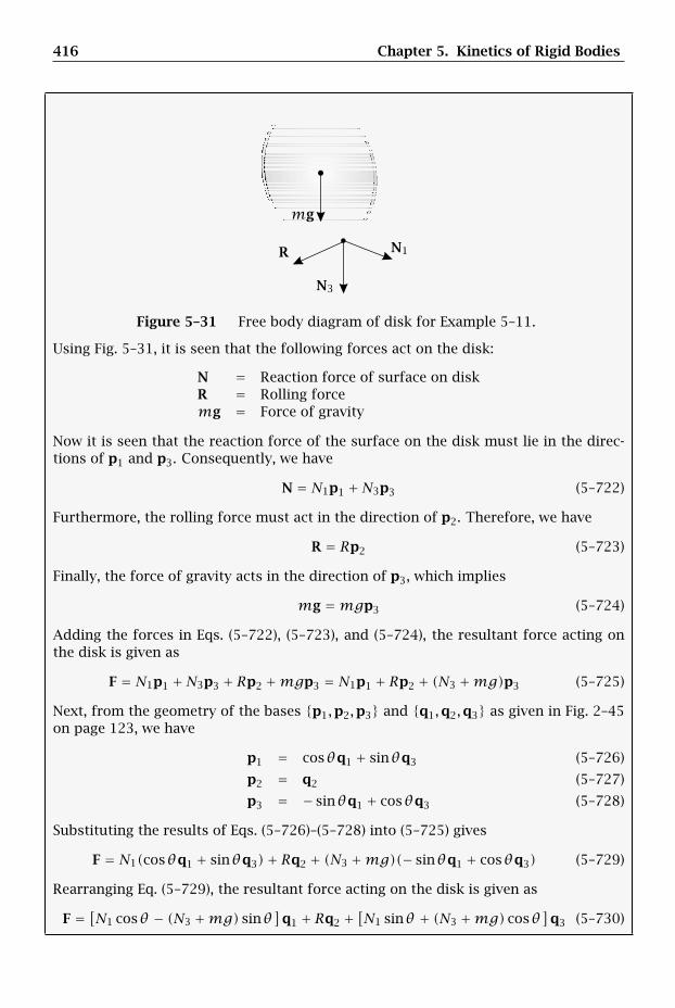
416 Chapter 5. Kinetics of Rigid Bodies
N1
N3
R
mg
Figure 5–31 Free body diagram of disk for Example 5–11.
Using Fig. 5–31, it is seen that the following forces act on the disk:
N = Reaction force of surface on diskR = Rolling forcemg = Force of gravity
Now it is seen that the reaction force of the surface on the disk must lie in the direc-tions of p1 and p3. Consequently, we have
N = N1p1 +N3p3 (5–722)
Furthermore, the rolling force must act in the direction of p2. Therefore, we have
R = Rp2 (5–723)
Finally, the force of gravity acts in the direction of p3, which implies
mg =mgp3 (5–724)
Adding the forces in Eqs. (5–722), (5–723), and (5–724), the resultant force acting onthe disk is given as
F = N1p1 +N3p3 + Rp2 +mgp3 = N1p1 + Rp2 + (N3 +mg)p3 (5–725)
Next, from the geometry of the bases p1,p2,p3 and q1,q2,q3 as given in Fig. 2–45on page 123, we have
p1 = cosθq1 + sinθq3 (5–726)
p2 = q2 (5–727)
p3 = − sinθq1 + cosθq3 (5–728)
Substituting the results of Eqs. (5–726)–(5–728) into (5–725) gives
F = N1(cosθq1 + sinθq3)+ Rq2 + (N3 +mg)(− sinθq1 + cosθq3) (5–729)
Rearranging Eq. (5–729), the resultant force acting on the disk is given as
F = [N1 cosθ − (N3 +mg) sinθ
]q1 + Rq2 +
[N1 sinθ + (N3 +mg) cosθ
]q3 (5–730)
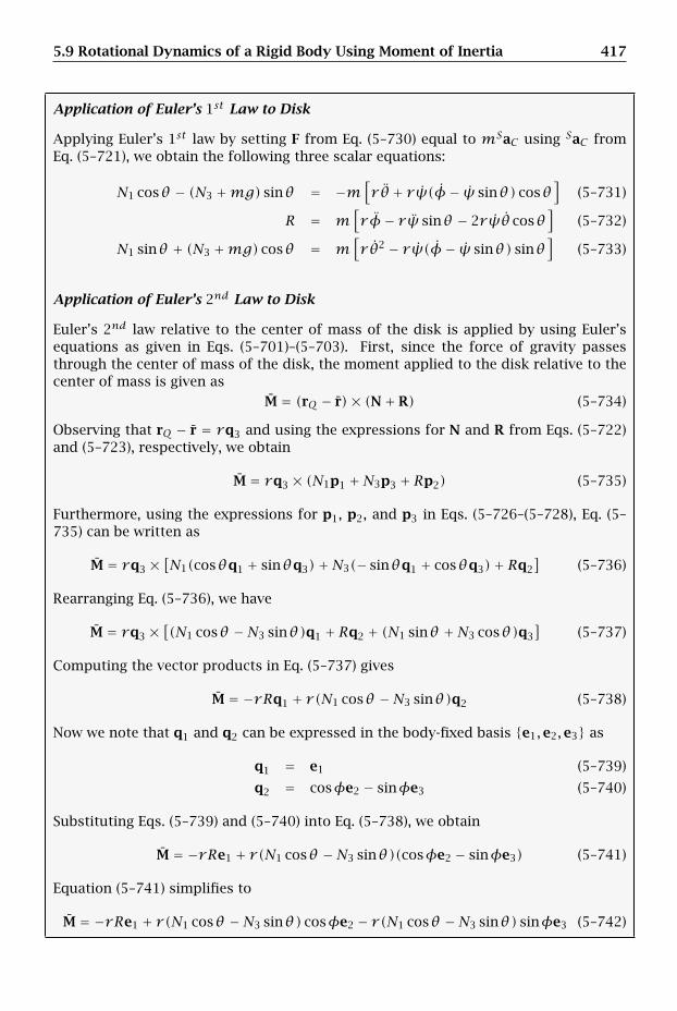
5.9 Rotational Dynamics of a Rigid Body Using Moment of Inertia 417
Application of Euler’s 1st Law to Disk
Applying Euler’s 1st law by setting F from Eq. (5–730) equal to mSaC using SaC fromEq. (5–721), we obtain the following three scalar equations:
N1 cosθ − (N3 +mg) sinθ = −m[r θ + rψ(φ− ψ sinθ) cosθ
](5–731)
R = m[rφ− rψ sinθ − 2rψθ cosθ
](5–732)
N1 sinθ + (N3 +mg) cosθ = m[r θ2 − rψ(φ− ψ sinθ) sinθ
](5–733)
Application of Euler’s 2nd Law to Disk
Euler’s 2nd law relative to the center of mass of the disk is applied by using Euler’sequations as given in Eqs. (5–701)–(5–703). First, since the force of gravity passesthrough the center of mass of the disk, the moment applied to the disk relative to thecenter of mass is given as
M = (rQ − r)× (N+ R) (5–734)
Observing that rQ − r = rq3 and using the expressions for N and R from Eqs. (5–722)and (5–723), respectively, we obtain
M = rq3 × (N1p1 +N3p3 + Rp2) (5–735)
Furthermore, using the expressions for p1, p2, and p3 in Eqs. (5–726–(5–728), Eq. (5–735) can be written as
M = rq3 ×[N1(cosθq1 + sinθq3)+N3(− sinθq1 + cosθq3)+ Rq2
](5–736)
Rearranging Eq. (5–736), we have
M = rq3 ×[(N1 cosθ −N3 sinθ)q1 + Rq2 + (N1 sinθ +N3 cosθ)q3
](5–737)
Computing the vector products in Eq. (5–737) gives
M = −rRq1 + r(N1 cosθ −N3 sinθ)q2 (5–738)
Now we note that q1 and q2 can be expressed in the body-fixed basis e1,e2,e3 as
q1 = e1 (5–739)
q2 = cosφe2 − sinφe3 (5–740)
Substituting Eqs. (5–739) and (5–740) into Eq. (5–738), we obtain
M = −rRe1 + r(N1 cosθ −N3 sinθ)(cosφe2 − sinφe3) (5–741)
Equation (5–741) simplifies to
M = −rRe1 + r(N1 cosθ −N3 sinθ) cosφe2 − r(N1 cosθ −N3 sinθ) sinφe3 (5–742)
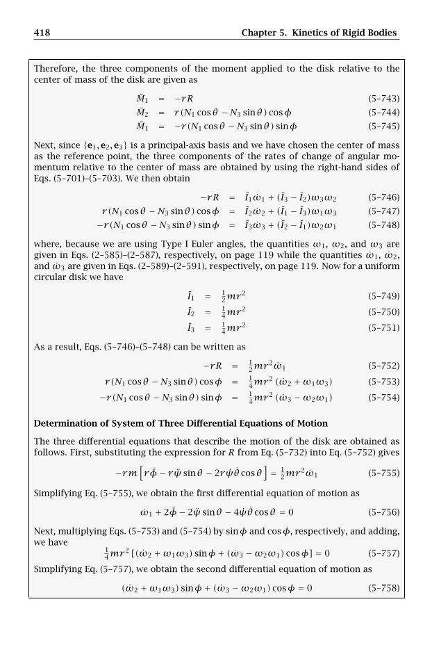
418 Chapter 5. Kinetics of Rigid Bodies
Therefore, the three components of the moment applied to the disk relative to thecenter of mass of the disk are given as
M1 = −rR (5–743)
M2 = r(N1 cosθ −N3 sinθ) cosφ (5–744)
M1 = −r(N1 cosθ −N3 sinθ) sinφ (5–745)
Next, since e1,e2,e3 is a principal-axis basis and we have chosen the center of massas the reference point, the three components of the rates of change of angular mo-mentum relative to the center of mass are obtained by using the right-hand sides ofEqs. (5–701)–(5–703). We then obtain
−rR = I1ω1 + (I3 − I2)ω3ω2 (5–746)
r(N1 cosθ −N3 sinθ) cosφ = I2ω2 + (I1 − I3)ω1ω3 (5–747)
−r(N1 cosθ −N3 sinθ) sinφ = I3ω3 + (I2 − I1)ω2ω1 (5–748)
where, because we are using Type I Euler angles, the quantities ω1, ω2, and ω3 aregiven in Eqs. (2–585)–(2–587), respectively, on page 119 while the quantities ω1, ω2,and ω3 are given in Eqs. (2–589)–(2–591), respectively, on page 119. Now for a uniformcircular disk we have
I1 = 12mr
2 (5–749)
I2 = 14mr
2 (5–750)
I3 = 14mr
2 (5–751)
As a result, Eqs. (5–746)–(5–748) can be written as
−rR = 12mr
2ω1 (5–752)
r(N1 cosθ −N3 sinθ) cosφ = 14mr
2 (ω2 +ω1ω3) (5–753)
−r(N1 cosθ −N3 sinθ) sinφ = 14mr
2 (ω3 −ω2ω1) (5–754)
Determination of System of Three Differential Equations of Motion
The three differential equations that describe the motion of the disk are obtained asfollows. First, substituting the expression for R from Eq. (5–732) into Eq. (5–752) gives
−rm[rφ− rψ sinθ − 2rψθ cosθ
]= 1
2mr2ω1 (5–755)
Simplifying Eq. (5–755), we obtain the first differential equation of motion as
ω1 + 2φ− 2ψ sinθ − 4ψθ cosθ = 0 (5–756)
Next, multiplying Eqs. (5–753) and (5–754) by sinφ and cosφ, respectively, and adding,we have
14mr
2 [(ω2 +ω1ω3) sinφ+ (ω3 −ω2ω1) cosφ] = 0 (5–757)
Simplifying Eq. (5–757), we obtain the second differential equation of motion as
(ω2 +ω1ω3) sinφ+ (ω3 −ω2ω1) cosφ = 0 (5–758)
5.10 Work and Energy for a Rigid Body 419
Furthermore, multiplying Eqs. (5–753) and (5–754) by cosφ and sinφ, respectively, andsubtracting, we obtain
r(N1 cosθ −N3 sinθ) = 14mr
2 [(ω2 +ω1ω3) cosφ+ (ω3 −ω2ω1) sinφ] (5–759)
Dropping the common factor of r from Eq. (5–759), we have
N1 cosθ −N3 sinθ = 14mr [(ω2 +ω1ω3) cosφ+ (ω3 −ω2ω1) sinφ] (5–760)
Then, solving Eq. (5–731) for N1 cosθ −N3 sinθ gives
N1 cosθ −N3 sinθ =mg sinθ −m[r θ + rψ(φ− ψ sinθ) cosθ
](5–761)
Substituting the result of Eq. (5–761) into Eq. (5–760) gives
mg sinθ −m[r θ + rψ(φ− ψ sinθ) cosθ
]= 1
4mr [(ω2 +ω1ω3) cosφ+ (ω3 −ω2ω1) sinφ](5–762)
Simplifying Eq. (5–762), we obtain the third differential equation of motion as
r (ω2 +ω1ω3) cosφ+ r (ω3 −ω2ω1) sinφ
+ r θ + rψ(φ− ψ sinθ) cosθ − 4g sinθ = 0(5–763)
The system of three differential equations of motion for the disk is then given as
ω1 + 2φ− 2ψ sinθ − 4ψθ cosθ = 0 (5–764)
(ω2 +ω1ω3) sinφ+ (ω3 −ω2ω1) cosφ = 0 (5–765)
r (ω2 +ω1ω3) cosφ+ r (ω3 −ω2ω1) sinφ+r θ + rψ(φ− ψ sinθ) cosθ − 4g sinθ = 0 (5–766)
where we again note that the quantities ω1, ω2, and ω3 are given in Eqs. (2–585)–(2–587), respectively, on page 119 while the quantities ω1, ω2, and ω3 are given inEqs. (2–589)–(2–591), respectively, on page 119.
5.10 Work and Energy for a Rigid Body
5.10.1 Kinetic Energy of a Rigid Body
Let R be a rigid body and let N be an inertial reference frame. Furthermore, let r bethe position of a point P onR and let Nv be the velocity of point P onR in the inertialreference frame N . Then the kinetic energy of a rigid body R in the inertial referenceN is defined as
NT = 12
∫RNv · Nvdm (5–767)

420 Chapter 5. Kinetics of Rigid Bodies
Now from Eq. (2–517) on page 106, we have
Nv = Nv+NωR × (r− r) (5–768)
Suppose now that we let ρ = r− r. Then Eq. (5–767) can be written as
NT = 12
∫R
[Nv+NωR × ρ
]·[Nv+NωR × ρ
]dm (5–769)
Expanding Eq. (5–769), we obtain
NT = 12
∫R
Nv · Nv+ 2Nv · NωR × ρ
+[NωR × ρ
]·[NωR × ρ
]dm
(5–770)
which can be rewritten as
NT = 12
∫RNv · Nvdm+
∫RNv ·
[NωR × ρ
]dm
+ 12
∫R
[NωR × ρ
]·[NωR × ρ
]dm
(5–771)
Since Nv is independent of the integral, Eq. (5–771) can be rewritten as
NT = 12Nv · Nv
∫Rdm+Nv ·
∫RNωR × ρdm
+ 12
∫R
[NωR × ρ
]·[NωR × ρ
]dm
(5–772)
Then, since ∫Rdm =m
Eq. (5–772) becomes
NT = 12mNv · Nv+Nv ·
∫RNωR × ρdm
+ 12
∫R
[NωR × ρ
]·[NωR × ρ
]dm
(5–773)
Next, because NωR is independent of the integral, the second term in Eq. (5–773) canbe written as
Nv ·∫RNωR × ρdm = Nv ·
[NωR ×
∫Rρdm
](5–774)
Furthermore, since ρ = r− r, we have∫Rρdm =
∫R(r− r)dm = 0 (5–775)
which implies that
Nv ·∫RNωR × ρdm = Nv ·
[NωR ×
∫Rρdm
]= 0 (5–776)
5.10 Work and Energy for a Rigid Body 421
In addition, we have12Nv · Nv
∫Rdm = 1
2mNv · Nv (5–777)
The kinetic energy of Eq. (5–773) then simplifies to
NT = 12mNv · Nv+ 1
2
∫R
[NωR × ρ
]·[NωR × ρ
]dm (5–778)
Furthermore, using the properties of the scalar triple product on page 9, we have[NωR × ρ
]·[NωR × ρ
]=[ρ× (NωR × ρ)
]· NωR (5–779)
Next, from the properties of the vector triple product on page 10, we have
ρ× (NωR × ρ) = (ρ · ρ)NωR −(ρ · NωR
)ρ (5–780)
Equation (5–780) can be written more conveniently in tensor form as
ρ× (NωR × ρ) = [(ρ · ρ)U− (ρ⊗ ρ)] · NωR (5–781)
where U is the identity tensor and(ρ · NωR)ρ = (ρ⊗ ρ) · NωR. Then, substituting
the result of Eq. (5–781) into (5–779), we obtain[NωR × ρ
]·[NωR × ρ
]=[(ρ · ρ)U− (ρ⊗ ρ)] · NωR
· NωR (5–782)
Consequently, the kinetic energy as given in Eq. (5–778) can be written as
NT = 12Nv · Nv
∫Rdm+ 1
2
∫R
[(ρ · ρ)U− (ρ⊗ ρ)] · NωR
· NωRdm (5–783)
Again using the fact that NωR is independent of the integral, the quantity NωR canbe taken out of the integral to give
NT = 12mNv · Nv+ 1
2
[∫R[(ρ · ρ)U− (ρ⊗ ρ)]dm
· NωR
]· NωR (5–784)
Recall from Eqs. (5–43) and (5–44) on page 327 that∫R[(ρ · ρ)U− (ρ⊗ ρ)]dm
· NωR = I
R · NωR = NH (5–785)
whereN
H is the angular momentum of the rigid body relative to the center of massin the inertial reference frame N . Substituting
NH from Eq. (5–785) into (5–784), the
kinetic energy of a rigid body can be written as
NT = 12m
Nv · Nv+ 12N
H · NωR (5–786)
The term12m
Nv · Nv (5–787)
is the translational kinetic energy of the center of mass of the rigid body in referenceframe N while the term
12N
H · NωR (5–788)
is the rotational kinetic energy relative to the center of mass of the rigid body in refer-ence frame N . Thus, Eq. (5–786) states that the kinetic energy of a rigid body is thesum of the translational kinetic energy of the center of mass of the rigid body and therotational kinetic energy about the center of mass of the rigid body. Equation (5–786)is referred to as Koenig’s decomposition of the kinetic energy of a rigid body.
422 Chapter 5. Kinetics of Rigid Bodies
5.10.2 Work-Energy Theorem for a Rigid Body
Computing the rate of change of kinetic energy using Eq. (5–786), we obtain
ddt
(NT
)= 1
2m[Nddt
(Nv
)· v+ v ·
Nddt
(Nv
)]
+ 12
[Nddt
(NH)· NωR +N
H ·Nddt
(NωR
)] (5–789)
Recall in Eq. (5–789) that, because NT is a scalar function, its rate of change is inde-pendent of the reference frame and, thus, can be computed arbitrarily in the inertialreference frame N . Equation (5–789) simplifies to
ddt
(NT
)=m
Nddt
(Nv
)· Nv+ 1
2
[Nddt
(NH)· NωR +N
H ·Nddt
(NωR
)](5–790)
Now focus on the two quantities in the second term of Eq. (5–790). In particular, usingEq. (5–684) on page 411, we have
Nddt
(NH)· NωR =
[IR · NαR +NωR ×
(IR · NωR
)]· NωR
=[IR · NαR
]· NωR +
[NωR ×
(IR · NωR
)]· NωR
(5–791)
Now it is observed that [NωR ×
(IR · NωR
)]· NωR = 0 (5–792)
Consequently,Nddt
(NH)· NωR =
[IR · NαR
]· NωR (5–793)
Furthermore, since the moment of inertia tensor is symmetric, we have[IR · NαR
]· NωR =
[IR · NωR
]· NαR (5–794)
However, we also have
NH ·
Nddt
(NωR
)=[IR · NωR
]· NαR (5–795)
As a result, the two quantities in the second term of Eq. (5–790) are equal, i.e., we have
Nddt
(NH)· NωR = N
H ·Nddt
(NωR
)(5–796)
Using the identity of Eq. (5–796) in (5–790), we obtain
ddt
(NT
)=m
Nddt
(Nv
)· Nv+
Nddt
(NH)· NωR (5–797)
Next, usingNd(Nv)/dt = Na, Eq. (5–797) can be written as
ddt
(NT
)=mNa · Nv+
Nddt
(NH)· NωR (5–798)
5.10 Work and Energy for a Rigid Body 423
Then, substituting Euler’s 1st law from Eq. (5–225) on page 355 and Euler’s 2nd lawfrom Eq. (5–237) from page 357, Eq. (5–798) becomes
ddt
(NT
)= F · Nv+ M · NωR (5–799)
Equation (5–799) is called the work-energy theorem for a rigid body.As it turns out, Eq. (5–799) is not the most useful form of the work-energy theorem
for a rigid body. The difficulty in applying Eq. (5–799) arises from the term F ·Nv. For-tunately, a more useful form of the work-energy theorem can be obtained as follows.From Eq. (5–218) we have
M =n∑i=1
(ri − r)× Fi + τ (5–800)
where F1, . . . ,Fn are the forces and the resultant pure torque, respectively, applied tothe rigid body. Substituting Eq. (5–800) into (5–799), we obtain
ddt
(NT
)= F · Nv+
⎡⎣ n∑i=1
(ri − r)× Fi + τ⎤⎦ · NωR (5–801)
Moving the quantity NωR inside the summation and recalling that the scalar productis commutative, Eq. (5–801) can be rearranged to give
ddt
(NT
)= F · Nv+
n∑i=1
NωR · [(ri − r)× Fi]+ τ · NωR (5–802)
Next, from the properties of the scalar triple product on page 9, we have
NωR · [(ri − r)× Fi] =[NωR × (ri − r)
]· Fi (5–803)
Furthermore, from Eq. (2–517) on page 106, we have
NωR × (ri − r) = Nvi −Nv (5–804)
Equation (5–803) then becomes
NωR · [(ri − r)× Fi] =[Nvi −Nv
]· Fi (5–805)
Substituting Eq. (5–805) into (5–802), we obtain
ddt
(NT
)= F · Nv+
n∑i=1
[Nvi −Nv
]· Fi + τ · NωR (5–806)
Furthermore, we note thatn∑i=1
Fi · Nv = F · Nv (5–807)
Substituting Eq. (5–807) into (5–806) gives
ddt
(NT
)= F · Nv+
n∑i=1
FiNvi − F · Nv+ τ · NωR (5–808)

424 Chapter 5. Kinetics of Rigid Bodies
Observing that the first and third terms in Eq. (5–808) cancel, we obtain
ddt
(NT
)=
n∑i=1
Fi · Nvi + τ · NωR (5–809)
Equation (5–809) is a more useful form of the work-energy theorem for a rigid body.The usefulness of Eq. (5–809) will be seen in examples that follow this section.
5.10.3 Principle of Work and Energy for a Rigid Body
Suppose now that we consider motion of a rigid bodyR over a time interval t ∈ [t1, t2].Then, integrating Eq. (5–809) from t1 to t2, we have
∫ t2t1
ddt
(NT
)dt =
∫ t2t1
⎧⎨⎩n∑i=1
Fi · Nvi + τ · NωR⎫⎬⎭dt (5–810)
Now we know that ∫ t2t1
n∑i=1
Fi · Nvidt = NWF12 (5–811)
where NWF12 is the work done by all forces acting on the rigid body in the inertialreference frame N . Furthermore, we have
∫ t2t1τ · NωRdt = NWτ
12 (5–812)
where NWτ12 is the work done by all of the pure torques acting on the rigid body.
Finally, ∫ t2t1
ddt
(NT
)dt = NT(t2)−NT(t1) (5–813)
Then, substituting the results of Eqs. (5–811), (5–812), and (5–813) into Eq. (5–810), weobtain
NT(t2)−NT(t1) = NWF12 +NWτ
12 (5–814)
which is called the principle of work and energy for a rigid body and states that thechange in kinetic energy of a rigid body in an inertial reference frame during a timeinterval t ∈ [t1, t2] is equal to the sum of the work done by all forces and all puretorques acting on the rigid body over that time interval.
5.10.4 Alternate Form of Work-Energy Theorem for a Rigid Body
Suppose now that we classify the forces that act on the rigid body as either conserva-tive or nonconservative such that
Fc1, . . . ,Fcp = Conservative forcesFnc1 , . . . ,Fncq = Nonconservative forces
5.10 Work and Energy for a Rigid Body 425
where p + q = n. Then the resultant force acting on the body can be written asn∑i=1
Fi =p∑i=1
Fci +q∑i=1
Fnci (5–815)
Similarly, suppose the resultant pure torque is decomposed into a conservative puretorque, τc , and a nonconservative pure torque, τnc , i.e.,
τ = τc + τnc (5–816)
The work-energy theorem for a rigid body as given in Eq. (5–809) can then be writtenas
ddt
(NT
)=
p∑i=1
Fci · Nvci +q∑i=1
Fnci · Nvnci + τc · NωR + τnc · NωR (5–817)
where Nvci (i = 1, . . . , p) and Nvnci (i = 1, . . . , q) are the velocities in reference frameN of the points of application on R of the conservative forces and nonconservativeforces, respectively. Recalling the power of a conservative force from Eq. (3–282), eachof the conservative forces Fci (i = 1,2, . . . , r ) satisfies the property
Fci · Nvci = −ddt
(NUi
)(i = 1,2, . . . , p) (5–818)
where NU1, . . . ,NUp are the potential energies of the conservative forces Fc1, . . . ,Fcp,respectively, in the inertial reference frame N . Similarly, using Eq. (5–207), the con-servative pure torque τc satisfies the property
τc · NωR = − ddt
(NV
)(5–819)
where NV is the potential energy of the conservative pure torque τc in the inertialreference frame N . Substituting Eqs. (5–818) and (5–819) into Eq. (5–817), we obtain
ddt
(NT
)=
p∑i=1
[− ddt
(NUi
)]+
q∑i=1
Fnci · Nvnci − ddt
(NV
)+ τnc · NωR (5–820)
Rearranging Eq. (5–820), we have
ddt
⎡⎣NT + p∑
i=1
NUi +NV
⎤⎦ = q∑
i=1
Fnci · Nvnci + τnc · NωR (5–821)
The quantity
NE = NT +NV +r∑i=1
NUi (5–822)
is called the total energy of the rigid body in the inertial reference frame N . In termsof the total energy, Eq. (5–821) can be written as
ddt
(NE
)=
q∑i=1
Fnci · Nvnci + τnc · NωR (5–823)
Equation (5–823) is called the alternate form of the work-energy theorem for a rigidbody and states that the rate of change of the total energy of a rigid body is equal tothe sum of the power produced by all nonconservative forces and the power producedby the resultant nonconservative pure torque acting the body.
426 Chapter 5. Kinetics of Rigid Bodies
5.10.5 Conservation of Energy for a Rigid Body
It is seen that if the power produced by all of the nonconservative forces and resultantnonconservative pure torque is zero, i.e.,
q∑i=1
Fnci · Nvnci + τnc · NωR = 0 (5–824)
thenddt
(NE
)= 0 (5–825)
which implies thatNE = constant (5–826)
In other words, the total energy of a rigid body will be conserved if the sum of thepower produced by the nonconservative forces and resultant nonconservative puretorque acting on the body is zero.
5.10.6 Alternate Form of Principle of Work and Energy for a Rigid Body
Suppose now that we consider the motion of a rigid body R over a time interval t ∈[t1, t2]. Then, integrating Eq. (5–823) from t1 to t2, we have
∫ t2t1
ddt
(NE
)dt =
∫ t2t1
⎧⎨⎩q∑i=1
Fnci · Nvnci + τnc · NωR⎫⎬⎭dt (5–827)
Now we know that ∫ t2t1
q∑i=1
Fnci · Nvnci dt = NWFnc12 (5–828)
where NWFnc12 is the work done by all of the nonconservative forces acting on therigid body in the inertial reference frame N . Furthermore, we have∫ t2
t1τnc · NωRdt = NWτnc
12 (5–829)
where NWτnc12 is the work done by the resultant nonconservative pure torque acting on
the rigid body. Finally, ∫ t2t1
ddt
(NE
)dt = NE(t2)−NE(t1) (5–830)
Then, substituting the results of Eqs. (5–828), (5–829), and (5–830) into Eq. (5–827), weobtain
NE(t2)−NE(t1) = NWFnc12 +NWτnc
12 (5–831)
Equation (5–831) is called the alternate form of the principle of work and energy fora rigid body and states that the change in total energy of a rigid body in an inertialreference frame during a time interval t ∈ [t1, t2] is equal to the sum of the work doneby all nonconservative forces and all nonconservative pure torques acting on the rigidbody over that time interval.
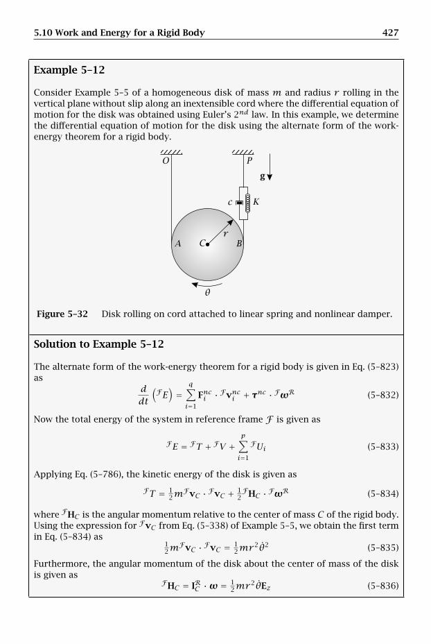
5.10 Work and Energy for a Rigid Body 427
Example 5–12
Consider Example 5–5 of a homogeneous disk of mass m and radius r rolling in thevertical plane without slip along an inextensible cord where the differential equation ofmotion for the disk was obtained using Euler’s 2nd law. In this example, we determinethe differential equation of motion for the disk using the alternate form of the work-energy theorem for a rigid body.
c
g
rA BC
K
O P
θ
Figure 5–32 Disk rolling on cord attached to linear spring and nonlinear damper.
Solution to Example 5–12
The alternate form of the work-energy theorem for a rigid body is given in Eq. (5–823)as
ddt
(FE)=
q∑i=1
Fnci · Fvnci + τnc · FωR (5–832)
Now the total energy of the system in reference frame F is given as
FE = FT + FV +p∑i=1
FUi (5–833)
Applying Eq. (5–786), the kinetic energy of the disk is given as
FT = 12m
FvC · FvC + 12FHC · FωR (5–834)
where FHC is the angular momentum relative to the center of mass C of the rigid body.Using the expression for FvC from Eq. (5–338) of Example 5–5, we obtain the first termin Eq. (5–834) as
12m
FvC · FvC = 12mr
2θ2 (5–835)
Furthermore, the angular momentum of the disk about the center of mass of the diskis given as
FHC = IRC ·ω = 12mr
2θEz (5–836)
428 Chapter 5. Kinetics of Rigid Bodies
The second term in Eq. (5–834) is then given as
12FHC · FωR = 1
2
[12mr
2θEz · θEz]= 1
4mr2θ2 (5–837)
Then, adding Eqs. (5–835) and (5–836), the kinetic energy of the disk is given as
FT = 12mr
2θ2 + 14mr
2θ2 = 34mr
2θ2 (5–838)
Now, the only conservative forces acting on the disk are those of the linear spring andgravity. Consequently, the potential energy in reference frame F is given as
FU = FUs + FUg (5–839)
where FUs and FUg are the potential energies due to the spring and gravity, respec-tively. The potential energy due to the linear spring is given from Eq. (3–296) on page193 as
FUs = K2( − 0
)2 (5–840)
where and 0 are the stretched and unstretched lengths of the spring, respectively.For this problem, we have
= rB − rP0 = L (5–841)
where rP is the position of the attachment point of the spring. Using rB − rP fromEq. (5–347), the position of point B is given as
rB − rP = (2rθ + L)Ex (5–842)
which implies that
− 0 = ‖rB − rP‖ − L = 2rθ + L− L = 2rθ (5–843)
The potential energy of the linear spring is then given as
FUs = K2 (2rθ)2 = 2Kr 2θ2 (5–844)
Next, because the force of gravity acts at the center of mass of the disk, the potentialenergy due to gravity is given as
FUg = −mg · rC (5–845)
Substituting the expressions formg and rC from Eqs. (5–325) and (5–342), respectively,we obtain
FUg = −mgEx · (rθEx) = −mgrθ (5–846)
The potential energy is then given as
FU = 2Kr 2θ2 −mgrθ (5–847)
and the total energy is given as
FE = FT + FU = 34mr
2θ2 + 2Kr 2θ2 −mgrθ (5–848)

5.10 Work and Energy for a Rigid Body 429
Computing the rate of change of FE we obtain
ddt
(FE)= 3
2mr2θθ + 4Kr 2θθ −mgrθ (5–849)
Next, because no pure torques are applied to the disk, we have
τnc · FωR = 0 (5–850)
Also, because the only nonconservative force that produces any power is that of thedamper, we obtain
q∑i=1
Fnci · Fvnci = Fd · vd = Fd · FvB (5–851)
Using the expressions for Fd and FvB from Eqs. (5–351) and (5–318), we have
q∑i=1
Fnci · Fvnci = −c(2r θ)3Ex · (2r θEx) = −16cr 4θ4 (5–852)
Then, setting d(FE)/dt in Eq. (5–849) equal to∑qi=1 Fnci · Fvnci from (5–852), we obtain
32mr
2θθ + 4Kr 2θθ −mgrθ = −16cr 4θ4 (5–853)
Rearranging this last expression, we obtain
θ[
32mr
2θ + 16cr 4θ3 + 4Kr 2θ −mgr]= 0 (5–854)
Observing that θ is not zero as a function of time, the differential equation of motionfor the disk is given as
32mr
2θ + 16cr 4θ3 + 4Kr 2θ −mgr = 0 (5–855)
It is seen that the result of Eq. (5–855) is identical to that of Eq. (5–366) as obtained onpage 367 in Example 5–5.
Example 5–13
A uniform slender rod of mass m and length l is hinged at one of its ends to a fixedpointO as shown in Fig. 5–33. Also attached to the rod at pointO are a torsional springwith spring constant K and a torsional damper with damping coefficient c. The springand damper both produce resistive pure torques. The spring is uncoiled when theangle θ shown in the figure is zero while the torque of the damper is proportional toθ. Knowing that gravity acts downward, determine the differential equation of motionfor the rod using the following methods: (a) Euler’s 2nd law using the hinge point asthe reference, (b) Euler’s laws using the center of mass of the rod as the reference, and
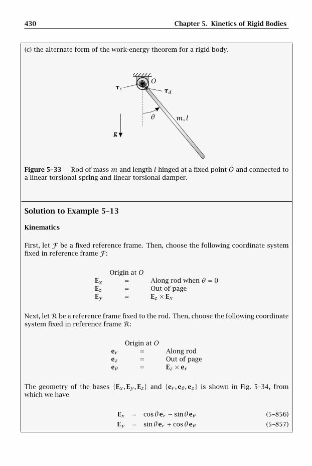
430 Chapter 5. Kinetics of Rigid Bodies
(c) the alternate form of the work-energy theorem for a rigid body.
g
m, l
O
θ
τdτs
Figure 5–33 Rod of massm and length l hinged at a fixed point O and connected toa linear torsional spring and linear torsional damper.
Solution to Example 5–13
Kinematics
First, let F be a fixed reference frame. Then, choose the following coordinate systemfixed in reference frame F :
Origin at OEx = Along rod when θ = 0Ez = Out of pageEy = Ez × Ex
Next, letR be a reference frame fixed to the rod. Then, choose the following coordinatesystem fixed in reference frame R:
Origin at Oer = Along rodez = Out of pageeθ = Ez × er
The geometry of the bases Ex,Ey,Ez and er ,eθ,ez is shown in Fig. 5–34, fromwhich we have
Ex = cosθer − sinθeθ (5–856)
Ey = sinθer + cosθeθ (5–857)
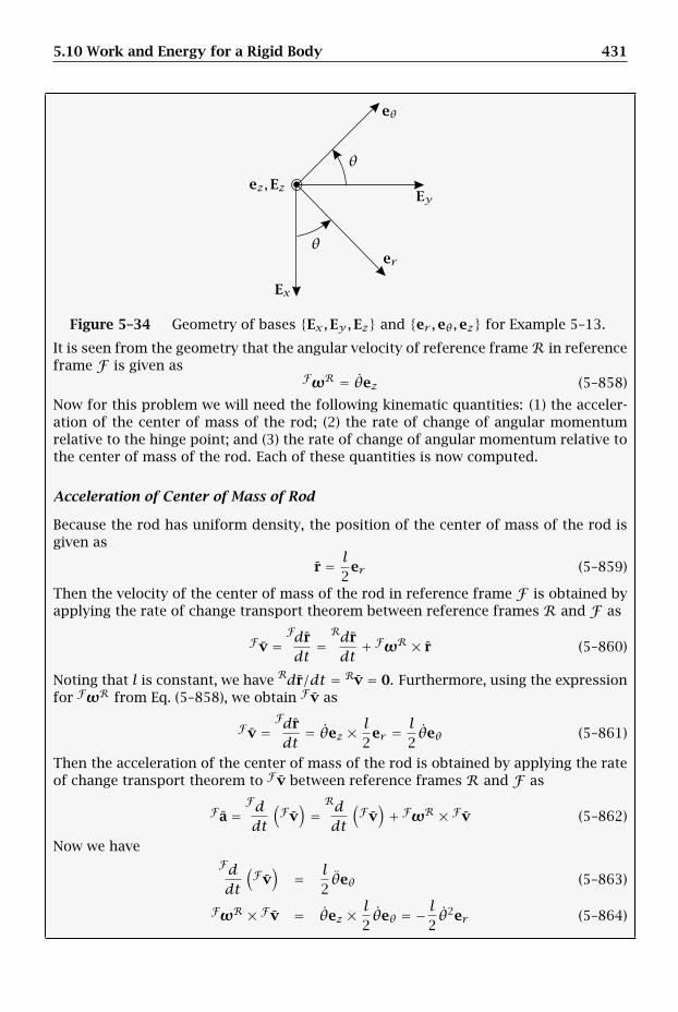
5.10 Work and Energy for a Rigid Body 431
er
eθ
Ex
Eyez,Ez
θ
θ
Figure 5–34 Geometry of bases Ex,Ey,Ez and er ,eθ,ez for Example 5–13.
It is seen from the geometry that the angular velocity of reference frameR in referenceframe F is given as
FωR = θez (5–858)
Now for this problem we will need the following kinematic quantities: (1) the acceler-ation of the center of mass of the rod; (2) the rate of change of angular momentumrelative to the hinge point; and (3) the rate of change of angular momentum relative tothe center of mass of the rod. Each of these quantities is now computed.
Acceleration of Center of Mass of Rod
Because the rod has uniform density, the position of the center of mass of the rod isgiven as
r = l2
er (5–859)
Then the velocity of the center of mass of the rod in reference frame F is obtained byapplying the rate of change transport theorem between reference frames R and F as
Fv =Fdrdt
=Rdrdt+ FωR × r (5–860)
Noting that l is constant, we have Rdr/dt = Rv = 0. Furthermore, using the expressionfor FωR from Eq. (5–858), we obtain Fv as
Fv =Fdrdt
= θez × l2er = l2 θeθ (5–861)
Then the acceleration of the center of mass of the rod is obtained by applying the rateof change transport theorem to Fv between reference frames R and F as
Fa =Fddt
(Fv)=Rddt
(Fv)+ FωR × Fv (5–862)
Now we haveFddt
(Fv)
= l2θeθ (5–863)
FωR × Fv = θez × l2 θeθ = − l2 θ2er (5–864)
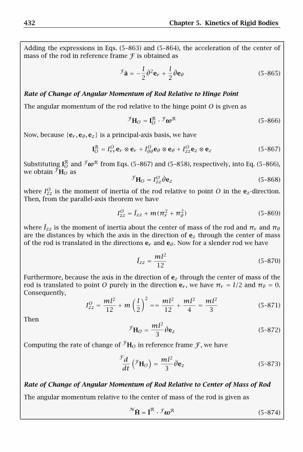
432 Chapter 5. Kinetics of Rigid Bodies
Adding the expressions in Eqs. (5–863) and (5–864), the acceleration of the center ofmass of the rod in reference frame F is obtained as
Fa = − l2θ2er + l2 θeθ (5–865)
Rate of Change of Angular Momentum of Rod Relative to Hinge Point
The angular momentum of the rod relative to the hinge point O is given as
FHO = IRO · FωR (5–866)
Now, because er ,eθ,ez is a principal-axis basis, we have
IRO = IOrrer ⊗ er + IOθθeθ ⊗ eθ + IOzzez ⊗ ez (5–867)
Substituting IRO and FωR from Eqs. (5–867) and (5–858), respectively, into Eq. (5–866),we obtain FHO as
FHO = IOzzθez (5–868)
where IOzz is the moment of inertia of the rod relative to point O in the ez-direction.Then, from the parallel-axis theorem we have
IOzz = Izz +m(π2r +π2
θ) (5–869)
where Izz is the moment of inertia about the center of mass of the rod and πr and πθare the distances by which the axis in the direction of ez through the center of massof the rod is translated in the directions er and eθ . Now for a slender rod we have
Izz = ml2
12(5–870)
Furthermore, because the axis in the direction of ez through the center of mass of therod is translated to point O purely in the direction er , we have πr = l/2 and πθ = 0.Consequently,
IOzz =ml2
12+m
(l2
)2
== ml2
12+ ml
2
4= ml
2
3(5–871)
ThenFHO = ml
2
3θez (5–872)
Computing the rate of change of FHO in reference frame F , we have
Fddt
(FHO
)= ml
2
3θez (5–873)
Rate of Change of Angular Momentum of Rod Relative to Center of Mass of Rod
The angular momentum relative to the center of mass of the rod is given as
NH = I
R · FωR (5–874)
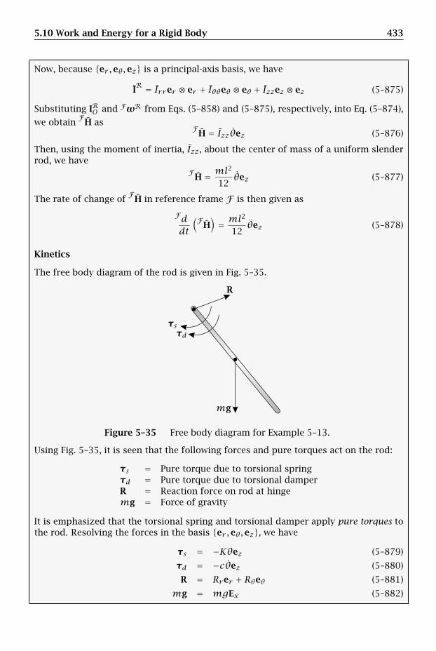
5.10 Work and Energy for a Rigid Body 433
Now, because er ,eθ,ez is a principal-axis basis, we have
IR = Irrer ⊗ er + Iθθeθ ⊗ eθ + Izzez ⊗ ez (5–875)
Substituting IRO and FωR from Eqs. (5–858) and (5–875), respectively, into Eq. (5–874),
we obtainF
H asF
H = Izzθez (5–876)
Then, using the moment of inertia, Izz, about the center of mass of a uniform slenderrod, we have
FH = ml
2
12θez (5–877)
The rate of change ofF
H in reference frame F is then given as
Fddt
(FH)= ml
2
12θez (5–878)
Kinetics
The free body diagram of the rod is given in Fig. 5–35.
R
mg
τdτs
Figure 5–35 Free body diagram for Example 5–13.
Using Fig. 5–35, it is seen that the following forces and pure torques act on the rod:
τs = Pure torque due to torsional springτd = Pure torque due to torsional damperR = Reaction force on rod at hingemg = Force of gravity
It is emphasized that the torsional spring and torsional damper apply pure torques tothe rod. Resolving the forces in the basis er ,eθ,ez, we have
τs = −Kθez (5–879)
τd = −cθez (5–880)
R = Rrer + Rθeθ (5–881)
mg = mgEx (5–882)
434 Chapter 5. Kinetics of Rigid Bodies
Then, using the expression for Ex from Eq. (5–856), the force of gravity is given as
mg =mg(cosθer − sinθeθ) =mg cosθer −mg sinθeθ (5–883)
It is extremely important to understand that the resultant force acting on the rod doesnot include the pure torques due to the torsional spring and the torsional damperbecause the pure torques do not arise from forces that act on the rod.
(a) Differential Equation Using Hinge as Reference Point
Because O is an inertially fixed point, we can apply Euler’s law relative to point O inreference frame F as
MO =Fddt
(FHO
)(5–884)
From the free body diagram of Fig. 5–35 we observe that the reaction R passes throughpoint O. Consequently, the moment relative to point O is due to gravity, the torsionalspring, and the torsional damper and is given as
MO = (rg − rO)×mg+ τs + τd (5–885)
Now we know that the force of gravity acts at the center of mass of the rod. Conse-quently,
rg = r = l2
er (5–886)
Furthermore, using the expression formg from Eq. (5–883) and noting that rO = 0, themoment due to gravity about point O is then computed as
(rg − rO)×mg = l2
er × (mg cosθer −mg sinθeθ) = −mgl2sinθez (5–887)
Then, using the expressions for τs and τd from Eqs. (5–879) and (5–880), respectively,we obtain the moment applied to the rod relative to the hinge point as
MO = −mgl2sinθez −Kθez − cθez
= −(mgl
2sinθ +Kθ + cθ
)ez
(5–888)
Then, setting MO in Eq. (5–888) equal toFd(FHO)/dt in Eq. (5–873), we obtain
−(mgl
2sinθ +Kθ + cθ
)= ml
2
3θ (5–889)
Rearranging this last expression, we obtain the differential equation of motion as
ml2
3θ + cθ +Kθ + mgl
2sinθ = 0 (5–890)
5.10 Work and Energy for a Rigid Body 435
(b) Differential Equation Using Center of Mass of Rod as Reference Point
Using the center of mass of the rod as the reference point, we need to apply both ofEuler’s laws. Applying Euler’s 1st law in reference frame F , we have
F =mFa (5–891)
Using the free body diagram of Fig. 5–35 we have
F = R+mg (5–892)
Furthermore, using the expressions for R and mg from Eqs. (5–881) and (5–883), re-spectively, the resultant force acting on the rod is given as
F = Rrer + Rθeθ +mg cosθer −mg sinθeθ (5–893)
which simplifies to
F = (Rr +mg cosθ)er + (Rθ −mg sinθ)eθ (5–894)
Setting F from Eq. (5–894) equal to mFa from Eq. (5–865), we obtain
(Rr +mg cosθ)er + (Rθ −mg sinθ)eθ = −ml2θ2er + ml2
θeθ (5–895)
which results in the following two scalar equations:
Rr +mg cosθ = −ml2θ2 (5–896)
Rθ −mg sinθ = ml2θ (5–897)
Next, we apply Euler’s 2nd law about the center of mass of the rod. First, themoment relative to the center of mass of the rod is given as
M =Fddt
(FH)
(5–898)
Now, because the force of gravity passes through the center of mass, the only momentsrelative to the center of mass are due to the reaction force, R; the pure torque of thetorsional spring τs ; and the pure torque of the torsional damper, τd. Recalling that apure torque is independent of the particular point on the rigid body, it can be translatedanywhere on the body without change. Consequently, the moment applied to the rodabout the center of mass of the rod is given as
M = (rR − r)× R+ τs + τd (5–899)
Because rR = rO = 0, we have
rR − r = − l2
er (5–900)
Therefore,
(rR − r)× R = − l2
er × (Rrer + Rθeθ) = − l2Rθez (5–901)

436 Chapter 5. Kinetics of Rigid Bodies
We then obtain
M = − l2Rθez −Kθez − cθez = −
(l2Rθ +Kθ + cθ
)ez (5–902)
Then, setting M in Eq. (5–902) withFd(FH)/dt from Eq. (5–878), we obtain
−(l2Rθ +Kθ + cθ
)= ml
2
12θ (5–903)
Rearranging this last expression, we obtain
ml2
12θ +Kθ + cθ = − l
2Rθ (5–904)
Equations (5–896), (5–897), and (5–904) can now be used to determine the differen-tial equation of motion. First, solving Eq. (5–897) for Rθ gives
Rθ = ml2θ +mg sinθ (5–905)
Next, substituting the expression for Rθ into Eq. (5–904), we obtain
ml2
12θ +Kθ + cθ = − l
2
[ml2θ +mg sinθ
](5–906)
Then, expanding the right-hand side of Eq. (5–906),
ml2
12θ +Kθ + cθ = −ml
2
4θ − mgl
2sinθ (5–907)
Rearranging Eq. (5–906), we obtain the differential equation of motion as
ml2
3θ + cθ +Kθ + mgl
2sinθ = 0 (5–908)
We note that Eq. (5–908) is the same as the result as obtained in part (a) above.
(c) Differential Equation Using Alternate Form of Work-Energy Theorem
For this problem we use the alternate form of the work-energy theorem for a rigid bodygiven in Eq. (5–823) on page 425 as
ddt
(FE)=
q∑i=1
Fnci · Fvnci + τnc · FωR (5–909)
Now the total energy of the system is given as
FE = FT + FU (5–910)
where FT and FU are the kinetic energy and potential energy, respectively, in referenceframe F . First, the kinetic energy of the rod in reference frame F is given as
FT = 12m
Fv · Fv+ 12F
H · FωR (5–911)
5.10 Work and Energy for a Rigid Body 437
Substituting the expression for Fv from Eq. (5–861) and the expression forF
H fromEq. (5–877) into (5–911), we obtain
FT = 12m
(12 θeθ · 1
2 θeθ)+ 1
2
(ml2
12θez · θez
)(5–912)
Simplifying Eq. (5–912) gives
FT = ml2
8θ2 + ml
2
24θ2 = ml
2
6θ2 (5–913)
Next, since the only conservative force acting on the rod is that due to gravity, whilethe only conservative pure torque acting on the rod is that due to the torsional spring,the potential energy of the system in reference frame F is given as
FU = FUg + FUs (5–914)
where FUg is the potential energy of gravity while FUs is the potential energy of thetorsional spring. Now, since gravity is a constant force, we have
FUg = −mg · r (5–915)
Using the expression formg from Eq. (5–883) and the expression for r from Eq. (5–859),we obtain FUg as
FUg = −(mg cosθer −mg sinθeθ) ·(l2 sinθer
)= −mgl
2cosθ (5–916)
Next, the potential energy due to the torsional spring, FUs , has the general form
FUs = 12K (θ − θ0)2 (5–917)
Because the torsional spring is uncoiled when θ = 0, we have that θ0 = 0. Therefore,
FUs = 12Kθ
2 (5–918)
Adding the results of Eqs. (5–916) and (5–918), we obtain the total potential energy ofthe system as
FU = FUg + FUs = −mgl2cosθ + 1
2Kθ2 (5–919)
Furthermore, adding Eqs. (5–913) and (5–919), the total energy of the system is givenas
FE = FT + FU = ml2
6θ2 − mgl
2cosθ + 1
2Kθ2 (5–920)
Computing the rate of change of FE, we obtain
ddt
(FE)= ml
2
3θθ + mgl
2θ sinθ +Kθθ (5–921)
Factoring out θ from Eq. (5–921) gives
ddt
(FE)= θ
[ml2
3θ + mgl
2sinθ +Kθ
](5–922)
438 Chapter 5. Kinetics of Rigid Bodies
Next, we need to determine the terms on the right-hand side of Eq. (5–909). It canbe seen that the only force other than gravity that acts on the rod is the reaction force,R. Furthermore, R acts at point O where the velocity is zero. Therefore,
q∑i=1
Fnci · Fvnci = R · 0 = 0 (5–923)
Also, the only pure torque other than the moment due to the torsional spring that actson the rod is that of the torsional damper. Therefore,
τnc · FωR = −cθez · θez = −cθ2 (5–924)
Then the power of all nonconservative forces and nonconservative pure torques isgiven as
q∑i=1
Fnci · Fvnci + τnc · FωR = −cθ2 (5–925)
Setting the result of Eq. (5–922) equal to the result of Eq. (5–925), we obtain
θ[ml2
3θ + mgl
2sinθ +Kθ
]= −cθ2 (5–926)
Since θ is not zero as a function of time, we can drop θ from both sides of the lastexpression. We then obtain
ml2
3θ + mgl
2sinθ +Kθ = −cθ (5–927)
Rearranging this last expression gives
ml2
3θ + cθ +Kθ + mgl
2sinθ = 0 (5–928)
which is the same result as obtained in parts (a) and (b).
Example 5–14
Consider Example 5–8 from page 384 of the imbalanced wheel rolling without slipalong an inclined plane of inclination angle β. Derive the differential equation of mo-tion for the wheel using the alternate form of the work-energy theorem for a rigidbody.
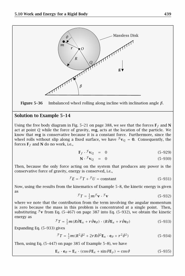
5.10 Work and Energy for a Rigid Body 439
Massless Disk
g
mr O
QR
β
θ
Figure 5–36 Imbalanced wheel rolling along incline with inclination angle β.
Solution to Example 5–14
Using the free body diagram in Fig. 5–21 on page 388, we see that the forces Ff and Nact at point Q while the force of gravity, mg, acts at the location of the particle. Weknow that mg is conservative because it is a constant force. Furthermore, since thewheel rolls without slip along a fixed surface, we have FvQ = 0. Consequently, theforces Ff and N do no work, i.e.,
Ff · FvQ = 0 (5–929)
N · FvQ = 0 (5–930)
Then, because the only force acting on the system that produces any power is theconservative force of gravity, energy is conserved, i.e.,
FE = FT + FU = constant (5–931)
Now, using the results from the kinematics of Example 5–8, the kinetic energy is givenas
FT = 12m
Fv · Fv (5–932)
where we note that the contribution from the term involving the angular momentumis zero because the mass in this problem is concentrated at a single point. Then,substituting Fv from Eq. (5–467) on page 387 into Eq. (5–932), we obtain the kineticenergy as
FT = 12m(RθEx + r θeθ) · (RθEx + r θeθ) (5–933)
Expanding Eq. (5–933) gives
FT = 12m(R
2θ2 + 2rRθ2Ex · eθ + r 2θ2) (5–934)
Then, using Eq. (5–447) on page 385 of Example 5–8), we have
Ex · eθ = Ex · (cosθEx + sinθEy) = cosθ (5–935)
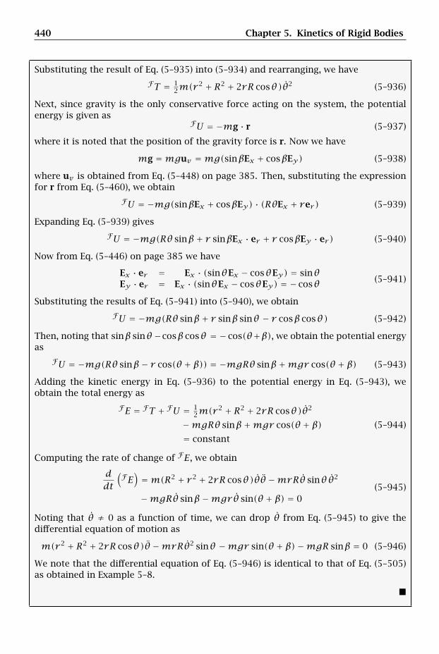
440 Chapter 5. Kinetics of Rigid Bodies
Substituting the result of Eq. (5–935) into (5–934) and rearranging, we have
FT = 12m(r
2 + R2 + 2rR cosθ)θ2 (5–936)
Next, since gravity is the only conservative force acting on the system, the potentialenergy is given as
FU = −mg · r (5–937)
where it is noted that the position of the gravity force is r. Now we have
mg =mguv =mg(sinβEx + cosβEy) (5–938)
where uv is obtained from Eq. (5–448) on page 385. Then, substituting the expressionfor r from Eq. (5–460), we obtain
FU = −mg(sinβEx + cosβEy) · (RθEx + rer ) (5–939)
Expanding Eq. (5–939) gives
FU = −mg(Rθ sinβ+ r sinβEx · er + r cosβEy · er ) (5–940)
Now from Eq. (5–446) on page 385 we have
Ex · er = Ex · (sinθEx − cosθEy) = sinθEy · er = Ex · (sinθEx − cosθEy) = − cosθ (5–941)
Substituting the results of Eq. (5–941) into (5–940), we obtain
FU = −mg(Rθ sinβ+ r sinβ sinθ − r cosβ cosθ) (5–942)
Then, noting that sinβ sinθ −cosβ cosθ = − cos(θ+β), we obtain the potential energyas
FU = −mg(Rθ sinβ− r cos(θ + β)) = −mgRθ sinβ+mgr cos(θ + β) (5–943)
Adding the kinetic energy in Eq. (5–936) to the potential energy in Eq. (5–943), weobtain the total energy as
FE = FT + FU = 12m(r
2 + R2 + 2rR cosθ)θ2
−mgRθ sinβ+mgr cos(θ + β)= constant
(5–944)
Computing the rate of change of FE, we obtain
ddt
(FE)=m(R2 + r 2 + 2rR cosθ)θθ −mrRθ sinθθ2
−mgRθ sinβ−mgrθ sin(θ + β) = 0(5–945)
Noting that θ ≠ 0 as a function of time, we can drop θ from Eq. (5–945) to give thedifferential equation of motion as
m(r 2 + R2 + 2rR cosθ)θ −mrRθ2 sinθ −mgr sin(θ + β)−mgR sinβ = 0 (5–946)
We note that the differential equation of Eq. (5–946) is identical to that of Eq. (5–505)as obtained in Example 5–8.

5.11 Impulse and Momentum for a Rigid Body 441
5.11 Impulse and Momentum for a Rigid Body
5.11.1 Linear Impulse and Linear Momentum for a Rigid Body
Recall from Euler’s 1st law that the translational motion of the center of mass of a rigidbody R is given from Eq. (5–225) as
F =mNa (5–947)
where N is an inertial reference frame. Integrating both sides of Eq. (5–947) from t1to t2, we have
∫ t2t1
Fdt =∫ t2t1mNadt =mNv(t2)−mNv(t1) = NG(t2)−NG(t1) (5–948)
where NG is the linear momentum of a rigid body as defined in Eq. (5–6) on page 323.Recalling the definition of a linear impulse from Chapter 3 we have
F = NG2 −NG1 (5–949)
where
F =∫ t2t1
Fdt (5–950)
is the linear impulse of the force F on the time interval from t1 to t2. Equation (5–949)is called the principle of linear impulse and momentum for a rigid body and states thatthe change in linear momentum of the rigid body is equal to the linear impulse appliedto the rigid body.
5.11.2 Angular Impulse and Angular Momentum for a Rigid Body
Suppose now that we integrate the result for the balance of angular momentum relativeto an arbitrary reference pointQ as given in Eq. (5–234) from an initial time t1 to a finaltime t2. We then have
∫ t2t1
MQdt −∫ t2t1(r− rQ)×mNaQdt =
∫ t2t1
Nddt
(NHQ
)dt (5–951)
It is seen that the right-hand side of Eq. (5–951) is given as
∫ t2t1
Nddt
(NHQ
)dt = NHQ(t2)−NHQ(t1) (5–952)
Furthermore, the first term on the left-hand side of Eq. (5–951) is the angular impulseon the time interval from t1 to t2, i.e.,
MQ =∫ t2t1
MQdt (5–953)
We then have
MQ −∫ t2t1(r− rQ)×mNaQdt = NHQ(t2)−NHQ(t1) (5–954)
442 Chapter 5. Kinetics of Rigid Bodies
Equation (5–954) is called the principle of angular impulse and angular momentum fora rigid body R relative to an arbitrary reference point Q.
Suppose now that we restrict our attention to motion relative to either a point Ofixed in an inertial reference frame N or the center of mass of a rigid body. In eitherof these two cases, it is seen that the second term in Eq. (5–954) is zero. Consequently,when the reference point is fixed in an inertial reference frame, we have
MO = NHO(t2)−NHO(t1) (5–955)
Equation (5–955) is called the principle of angular impulse and angular momentum fora rigid body relative to a point fixed in an inertial reference frame N . Similarly, whenthe reference point is the center of mass, we have
ˆM = NH(t2)−N
H(t1) (5–956)
Equation (5–956) is called the principle of angular impulse and angular momentum fora rigid body relative to the center of mass of the rigid body in an inertial referenceframe N .
Example 5–15
A sphere of mass m and radius r is set in motion by placing it in contact with aplane inclined at an angle β with the horizontal and giving its center of mass an initialvelocity v0 in the direction of the incline as shown in Fig. 5–37. Knowing that thecoefficient of sliding friction between the sphere and the incline is µ and that gravityacts downward, determine (a) the velocity of the center of mass of the sphere whensliding stops and rolling begins, (b) the angular velocity of the sphere when slidingstops and rolling begins, and (c) the time at which the sphere stops sliding and beginsrolling.
Friction (µ)
g
v0
r
O
P
β
Figure 5–37 Sphere sliding along a surface inclined at an angle β with the horizontal.
5.11 Impulse and Momentum for a Rigid Body 443
Solution to Example 5–15
Kinematics
It is convenient to analyze this problem using a fixed reference frame, F . Correspond-ing to F , the following coordinate system is chosen to describe the motion:
Origin at Owhen t = 0
Ex = Up inclineEz = Into pageEy = Ez × Ex
It is important to note for this problem that, while the origin of the above chosencoordinate system is a fixed point, the center of mass of the sphere (located at pointO) is a moving point. In terms of the basis Ex,Ey,Ez, the position of the center ofmass of the sphere is given as
r = rO = xEx (5–957)
The velocity of the center of mass of the disk is then given as
Fv = xEx ≡ vEx (5–958)
The acceleration of the center of mass of the disk is then obtained as
Fa = xEx (5–959)
Furthermore, the position of the point of contact of the sphere with the incline is givenas
rP = xEx + rEy (5–960)
Now, because the sphere rotates about an axis orthogonal to the page, the angularvelocity of the sphere in reference frame F can be written as
FωR =ωEz (5–961)
The velocity of the point of contact on the sphere, denoted FvP , is then determinedusing Eq. (2–517) on page 106 as
FvP = Fv+ FωR × (rP − r) (5–962)
Now from Eqs. (5–957) and (5–960) we have
rP − r = rEy (5–963)
Substituting FωR and rP − r from Eqs. (5–961) and (5–963), respectively, into Eq. (5–962), we obtain
FvP = vEx +ωEz × (rEy) = (v − rω)Ex (5–964)
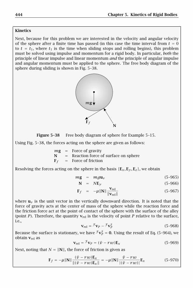
444 Chapter 5. Kinetics of Rigid Bodies
Kinetics
Next, because for this problem we are interested in the velocity and angular velocityof the sphere after a finite time has passed (in this case the time interval from t = 0to t = t1, where t1 is the time when sliding stops and rolling begins), this problemmust be solved using impulse and momentum for a rigid body. In particular, both theprinciple of linear impulse and linear momentum and the principle of angular impulseand angular momentum must be applied to the sphere. The free body diagram of thesphere during sliding is shown in Fig. 5–38.
FfN
mg
Figure 5–38 Free body diagram of sphere for Example 5–15.
Using Fig. 5–38, the forces acting on the sphere are given as follows:
mg = Force of gravityN = Reaction force of surface on sphereFf = Force of friction
Resolving the forces acting on the sphere in the basis Ex,Ey,Ez, we obtain
mg = mguv (5–965)
N = NEy (5–966)
Ff = −µ‖N‖ vrel
‖vrel‖(5–967)
where uv is the unit vector in the vertically downward direction. It is noted that theforce of gravity acts at the center of mass of the sphere while the reaction force andthe friction force act at the point of contact of the sphere with the surface of the alley(point P ). Therefore, the quantity vrel is the velocity of point P relative to the surface,i.e.,
vrel = FvP − FvSP (5–968)
Because the surface is stationary, we have FvSP = 0. Using the result of Eq. (5–964), weobtain vrel as
vrel = FvP = (v − rω)Ex (5–969)
Next, noting that N = ‖N‖, the force of friction is given as
Ff = −µ‖N‖(v − rω)Ex‖(v − rω)Ex‖
= −µ‖N‖ v − rω|(v − rω)|Ex (5–970)
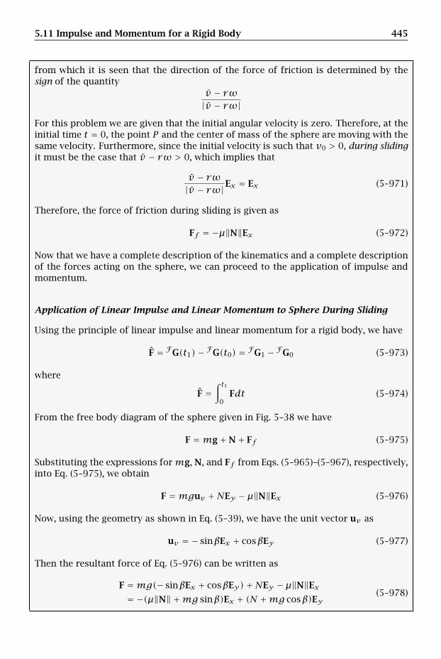
5.11 Impulse and Momentum for a Rigid Body 445
from which it is seen that the direction of the force of friction is determined by thesign of the quantity
v − rω|v − rω|
For this problem we are given that the initial angular velocity is zero. Therefore, at theinitial time t = 0, the point P and the center of mass of the sphere are moving with thesame velocity. Furthermore, since the initial velocity is such that v0 > 0, during slidingit must be the case that v − rω > 0, which implies that
v − rω|v − rω|Ex = Ex (5–971)
Therefore, the force of friction during sliding is given as
Ff = −µ‖N‖Ex (5–972)
Now that we have a complete description of the kinematics and a complete descriptionof the forces acting on the sphere, we can proceed to the application of impulse andmomentum.
Application of Linear Impulse and Linear Momentum to Sphere During Sliding
Using the principle of linear impulse and linear momentum for a rigid body, we have
F = FG(t1)− FG(t0) = FG1 − FG0 (5–973)
where
F =∫ t1
0Fdt (5–974)
From the free body diagram of the sphere given in Fig. 5–38 we have
F =mg+N+ Ff (5–975)
Substituting the expressions formg, N, and Ff from Eqs. (5–965)–(5–967), respectively,into Eq. (5–975), we obtain
F =mguv +NEy − µ‖N‖Ex (5–976)
Now, using the geometry as shown in Eq. (5–39), we have the unit vector uv as
uv = − sinβEx + cosβEy (5–977)
Then the resultant force of Eq. (5–976) can be written as
F =mg(− sinβEx + cosβEy)+NEy − µ‖N‖Ex= −(µ‖N‖ +mg sinβ)Ex + (N +mg cosβ)Ey
(5–978)
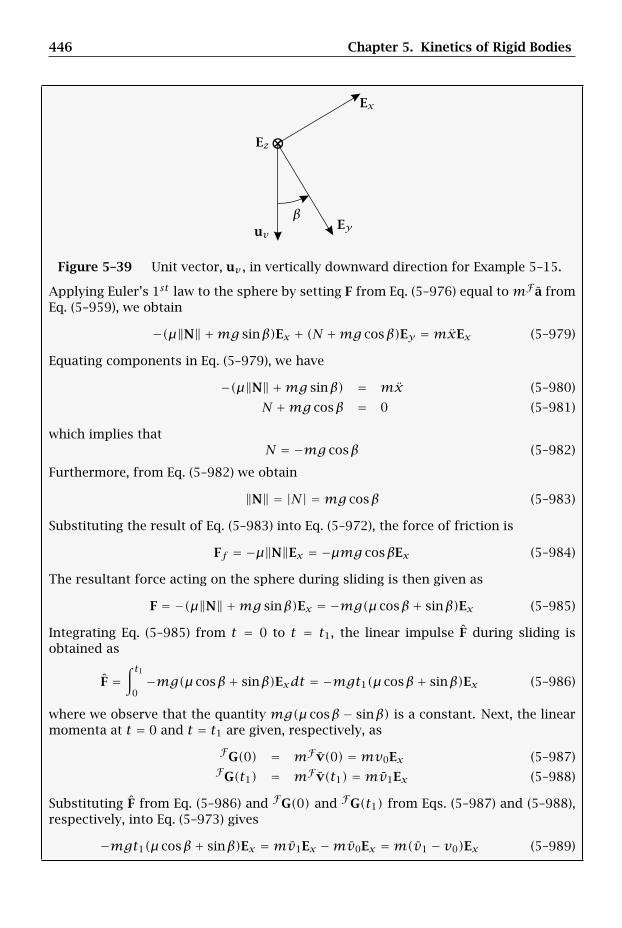
446 Chapter 5. Kinetics of Rigid Bodies
⊗
Ex
Ey
Ez
uv
β
Figure 5–39 Unit vector, uv , in vertically downward direction for Example 5–15.
Applying Euler’s 1st law to the sphere by setting F from Eq. (5–976) equal tomFa fromEq. (5–959), we obtain
−(µ‖N‖ +mg sinβ)Ex + (N +mg cosβ)Ey =mxEx (5–979)
Equating components in Eq. (5–979), we have
−(µ‖N‖ +mg sinβ) = mx (5–980)
N +mg cosβ = 0 (5–981)
which implies thatN = −mg cosβ (5–982)
Furthermore, from Eq. (5–982) we obtain
‖N‖ = |N| =mg cosβ (5–983)
Substituting the result of Eq. (5–983) into Eq. (5–972), the force of friction is
Ff = −µ‖N‖Ex = −µmg cosβEx (5–984)
The resultant force acting on the sphere during sliding is then given as
F = −(µ‖N‖ +mg sinβ)Ex = −mg(µ cosβ+ sinβ)Ex (5–985)
Integrating Eq. (5–985) from t = 0 to t = t1, the linear impulse F during sliding isobtained as
F =∫ t1
0−mg(µ cosβ+ sinβ)Exdt = −mgt1(µ cosβ+ sinβ)Ex (5–986)
where we observe that the quantity mg(µ cosβ − sinβ) is a constant. Next, the linearmomenta at t = 0 and t = t1 are given, respectively, as
FG(0) = mFv(0) =mv0Ex (5–987)FG(t1) = mFv(t1) =mv1Ex (5–988)
Substituting F from Eq. (5–986) and FG(0) and FG(t1) from Eqs. (5–987) and (5–988),respectively, into Eq. (5–973) gives
−mgt1(µ cosβ+ sinβ)Ex =mv1Ex −mv0Ex =m(v1 − v0)Ex (5–989)
5.11 Impulse and Momentum for a Rigid Body 447
Equation (5–989) simplifies to
v1 − v0 = −gt1(µ cosβ+ sinβ) (5–990)
Equation (5–990) is the first of three equations that will be used to obtain the solutionto this problem. It is noted that this equation has two unknowns: v1 and t1.
Application of Angular Impulse and Angular Momentum to Sphere During Sliding
For this problem there are no convenient fixed points about which to apply angularimpulse and angular momentum. Consequently, we must apply angular impulse andangular momentum about the center of mass of the sphere. From the principle ofangular impulse and angular momentum, we have
ˆM = FH(t1)− F
H(0) = FH1 − F
H0 (5–991)
where
ˆM =∫ t1
0Mdt (5–992)
From the free body diagram of Fig. 5–38 we see that the forcesmg and N pass throughthe center of mass of the sphere. Consequently, the resultant moment about the centerof mass is due entirely to the friction force and is given as
M = (rP − r)× Ff (5–993)
where we note that the friction force acts at point P . Substituting rP − bfrbar fromEq. (5–963) and Ff from Eq. (5–984) into (5–993) gives
M = rEy × (−µmg cosβEx) = rµmg cosβEz (5–994)
Integrating Eq. (5–994) from t = 0 to t = t1, we obtain the angular impulse as
ˆM =∫ t1
0rµmg cosβEzdt = rµmgt1 cosβEz (5–995)
where we observe that the quantity rµmgt1 cosβ and the unit vector Ez are both con-stant. Next, the angular momentum of the sphere relative to the center of mass of thesphere is given as
FH = I
R · FωR (5–996)
Now, in terms of the basis Ex,Ey,Ez, we have
IR = IxxEx ⊗ Ex + IyyEy ⊗ Ey + IzzEz ⊗ Ez (5–997)
Then, substituting the moment of inertia tensor from Eq. (5–997) and the angular ve-locity from Eq. (5–961) into (5–996), we obtain
FH =
(IxxEx ⊗ Ex + IyyEy ⊗ Ey + IzzEz ⊗ Ez
)·ωEz = IzzωEz (5–998)

448 Chapter 5. Kinetics of Rigid Bodies
Using the expression forF
H from Eq. (5–998), the angular momenta relative to thecenter of mass of the sphere at t = 0 and t = t1 are given, respectively, as
FH(0) = Izzω(0)Ez = Izzω0Ez (5–999)
FH(t1) = Izzω(t1)Ez = Izzω1Ez (5–1000)
Because the sphere is homogeneous, we have
Izz = 25mr
2
Consequently,
FH0 = 2
5mr2ω0Ez (5–1001)
FH1 = 2
5mr2ω1Ez (5–1002)
SubstitutingF
H0,F
H1, and ˆM from Eqs. (5–1001), (5–1002), and (5–995), respectively,into Eq. (5–991), we obtain
rµmgt1 cosβEz = 25mr
2ω1Ez − 25mr
2ω0Ez = 25mr
2(ω1 −ω0)Ez (5–1003)
Finally, because the initial angular velocity is zero, Eq. (5–1003) simplifies to
rµmgt1 cosβEz = 25mr
2ω1Ez (5–1004)
which givesµgt1 cosβ = 2
5rω1 (5–1005)
This is the second of three equations that will be used to obtain the solution to thisproblem. It is noted that this equation has two unknowns: ω1 and t1.
Kinematic Constraint at Sliding/Rolling Transition Point
Recall from Eq. (2–531) on page 109 that a rigid body will roll along a fixed surface ifthe velocity of the point on the body in contact with the fixed surface is zero. Becausein this problem we are interested in the point where sliding stops and rolling begins, itis required that the velocity of the point of contact, P , be zero at t = t1, i.e., we requirethat
FvP (t1) = 0 (5–1006)
Now, using Eq. (2–517) from page 106 at t = t1, we can express FvP (t1) in terms of thevelocity of the center of mass of the sphere as
Fv(t1) = FvP (t1)+ FωR(t1)× (r(t1)− rP (t1)) (5–1007)
We note from Eqs. (5–961) and (5–963) that
r(t1)− rP (t1) = −rEy (5–1008)FωR(t1) = ω1Ez (5–1009)
5.11 Impulse and Momentum for a Rigid Body 449
Then, substituting FvP (t1) from Eq. (5–1006) and using the expressions in Eqs. (5–1008) and (5–1009), we obtain
Fv(t1) =ω1Ez × (−rEy) = rω1Ex (5–1010)
Furthermore, noting that Fv(t1) = v1Ex , Eq. (5–1010) simplifies to
v1Ex = rω1Ex (5–1011)
We then obtainv1 = rω1 (5–1012)
This is the third of three equations that will be used to obtain the solution to thisproblem. It is noted that this equation has two unknowns: v1 and ω1.
(a) Velocity of Center of Mass of Sphere When Sliding Stops and Rolling Begins
Solving Eq. (5–1005) for t1, we obtain
t1 = 2rω1
5µg cosβ(5–1013)
Next, substituting v1 from Eq. (5–1012) into (5–1013), we have
t1 = 2v1
5µg cosβ(5–1014)
Then, substituting t1 from Eq. (5–1014) into (5–990) gives
v1 − v0 = −g 2v1
5µg cosβ(µ cosβ+ sinβ) (5–1015)
Solving Eq. (5–1015) for v1, we obtain
v1 = 5µv0 cosβ7µ cosβ+ 2 sinβ
(5–1016)
Therefore, the velocity of the center of mass of the sphere when sliding stops androlling begins is given as
Fv1 = 5µv0 cosβ7µ cosβ+ 2 sinβ
Ex (5–1017)
(b) Angular Velocity of Sphere When Sliding Stops and Rolling Begins
Substituting v1 from Eq. (5–1016) into (5–1012), we obtain
rω1 = 5µv0 cosβ7µ cosβ+ 2 sinβ
(5–1018)
Solving Eq. (5–1018) for ω1 gives
ω1 = 5µv0 cosβr(7µ cosβ+ 2 sinβ)
(5–1019)
Therefore, the angular velocity of the sphere when sliding stops and rolling begins isgiven as
FωR(t1) =ω1Ez = 5µv0 cosβr(7µ cosβ+ 2 sinβ)
Ez (5–1020)
450 Chapter 5. Kinetics of Rigid Bodies
(c) Time at Which Sliding Stops and Rolling Begins
Substituting v1 from Eq. (5–1016) into (5–1014), we obtain the time at which slidingstops and rolling begins as
t1 = 2v0
g(7µ cosβ+ 2 sinβ)(5–1021)
5.12 Collision of Rigid Bodies
In Section 4.8, we developed a model for the collision between two objects under theassumption that the objects were particles. It is clear that in a real collision the objectsare not particles, i.e., the objects have a nonzero size and have some associated shape.In order to account for objects with nonzero dimension, in this section we extend thediscussion of Section 4.8 to the collision between two rigid bodies.
5.12.1 Collision Model
Consider a collision between two rigid bodies R1 and R2. Assume that, during thecollision, the positions and orientations of the two bodies do not change and that thetwo rigid bodies are in contact at a single point P as shown in Fig. 5–40.Then, let
r1 = Position of Center of Mass of R1 During Collisionr2 = Position of Center of Mass of R2 During CollisionrP = Position of Point of Contact P During Collision
Also, let n be the unit normal to the tangent planes of B1 and B2 at point P , and let uand w be two unit vectors that lie in the plane orthogonal to n such that u,w,n formsa right-handed system. Then, denoting t0 and t1 as the times at the beginning and theend of the collision, we can define the following quantities in an inertial referenceframe N :
NvR1 = Velocity of center of mass of R1 at t0NvR2 = Velocity of center of mass of R2 at t0NvR1
P = Velocity of point P on R1 at t0NvR2
P = Velocity of point P on R2 at t0(NvR1
)′ = Velocity of center of mass of R1 at t1(NvR2
)′ = Velocity of center of mass of R2 at t1(NvR1
P
)′ = Velocity of point P on R1 at t1(NvR2
P
)′ = Velocity of point P on R2 at t1N
HR1 = Angular momentum relative to center of mass of R1 at t0
NHR2 = Angular Momentum relative to center of mass of R2 at t0(NHR1)′ = Angular Momentum relative to center of mass of R1 at t1(N
HR2)′ = Angular Momentum relative to center of mass of R2 at t1
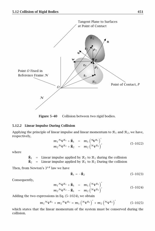
5.12 Collision of Rigid Bodies 451
Tangent Plane to Surfacesat Point of Contact
Point O Fixed in
N
R1
R2
Reference Frame N
Point of Contact, P
n
r1
r2
rP
u
w
O
P
ρ1
ρ2
Figure 5–40 Collision between two rigid bodies.
5.12.2 Linear Impulse During Collision
Applying the principle of linear impulse and linear momentum toR1 andR2, we have,respectively,
m1NvR1 + R1 = m1
(NvR1
)′m2
NvR2 + R2 = m2
(NvR2
)′ (5–1022)
where
R1 = Linear impulse applied by R2 to R1 during the collisionR2 = Linear impulse applied by R1 to R2 During the collision
Then, from Newton’s 3rd law we have
R1 = −R2 (5–1023)
Consequently,
m1NvR1 + R1 = m1
(NvR1
)′m2
NvR2 − R1 = m2
(NvR2
)′ (5–1024)
Adding the two expressions in Eq. (5–1024), we obtain
m1NvR1 +m2
NvR2 =m1
(NvR1
)′ +m2
(NvR2
)′(5–1025)
which states that the linear momentum of the system must be conserved during thecollision.
452 Chapter 5. Kinetics of Rigid Bodies
5.12.3 Angular Impulse During Collision
Applying the principle of angular impulse and angular momentum to R1 and R2, wehave
NHR1 + ˆM1 =
(NHR1)′
NHR2 + ˆM2 =
(NHR2)′ (5–1026)
where
ˆM1 = Angular impulse applied by R2 to R1 relative to center of mass ofR1 during the collision
ˆM2 = Angular impulse applied by R1 to R2 relative to center of mass ofR2 during the collision
We note that the angular impulses ˆM1 and ˆM2 are computed as
ˆM1 = ρ1 × R1ˆM1 = ρ2 × R2
(5–1027)
andρ1 = rP − r1
ρ2 = rP − r2(5–1028)
5.12.4 Coefficient of Restitution
Similar to the collision between two particles, the collision between two rigid bodiesis governed by the material properties of each body at the point of contact. Theseproperties are subsumed into an ad hoc scalar parameter, e, called the coefficient ofrestitution. In particular, the coefficient of restitution condition for the collision be-tween two rigid bodies is given as
e =(NvR2
P
)′ · n−(NvR1
P
)′ · n
NvR1P · n−NvR2
P · n(5–1029)
Equation (5–1029) is called Poisson’s hypothesis.
5.12.5 Solving for Post-Impact Velocities and Angular Velocities
Unlike the collision between two particles, general expressions for the post-impactconditions of two colliding rigid bodies cannot be obtained. In particular, the post-impact angular velocities and velocities of the centers of mass must be obtained foreach problem by solving Eqs. (5–1024), (5–1025), (5–1026), and (5–1029). The ease ordifficulty in solving these equations is highly problem-dependent. It is noted that, forthe case where the motion is planar, Eqs. (5–1024), (5–1025), (5–1026), and (5–1029)simplify drastically and become much more tractable. To demonstrate the applicabilityof the collision model derived in this section, in the next two examples we considerproblems involving collisions with rigid bodies in planar motion.

5.12 Collision of Rigid Bodies 453
Example 5–16
A uniform slender rod of massm and length l is released from rest at an angle θ abovea horizontal surface as shown in Fig. 5–41. After release, the rod descends a distanceh under the influence of gravity until its lowest point (i.e., point B) strikes the surface.Knowing that the coefficient of restitution between the rod and the surface is e (where0 ≤ e ≤ 1), determine (a) the velocity of the center of mass of the rod the instant beforethe rod strikes the surface and (b) the angular velocity and the velocity of the centerof mass of the rod the instant after the rod strikes the surface.
g
m, l
h
A
B
C θ
Figure 5–41 Rod striking fixed horizontal surface after descending from a height habove the surface.
Solution to Example 5–16
Kinematics
First, let F be a fixed reference frame. Then, choose the following coordinate systemfixed in reference frame F :
Origin at point Cwhen t = 0
Ex = Along gEz = Out of pageEy = Ez × Ex
Then, the velocity of the center of mass of the rod is given as
Fv = vxEx + vyEy (5–1030)
Next, denoting the reference frame of the rod by R and observing that the motion isplanar, the angular velocity of the rod in reference frame F is given as
FωR =ωEz (5–1031)
Finally, the velocity of point B located at the lower end of the rod is obtained usingEq. (2–517) on page 106) as
FvB = Fv+ FωR × (rB − r) (5–1032)
Now, the direction from the center of mass of the rod to point B on the rod is denoteder and is shown in Fig. 5–42.
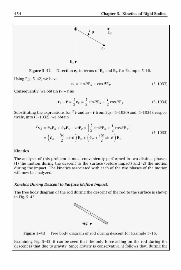
454 Chapter 5. Kinetics of Rigid Bodies
er
Ex
Eyθ
Figure 5–42 Direction er in terms of Ex and Ey for Example 5–16.
Using Fig. 5–42, we haveer = sinθEx + cosθEy (5–1033)
Consequently, we obtain rB − r as
rB − r = l2
er = l2 sinθEx + l2 cosθEy (5–1034)
Substituting the expressions for Fv and rB− r from Eqs. (5–1030) and (5–1034), respec-tively, into (5–1032), we obtain
FvB = vxEx + vyEy +ωEz ×[l2
sinθEx + l2 cosθEy
]
=(vx − lω2 cosθ
)Ex +
(vy + lω2 sinθ
)Ey
(5–1035)
Kinetics
The analysis of this problem is most conveniently performed in two distinct phases:(1) the motion during the descent to the surface (before impact) and (2) the motionduring the impact. The kinetics associated with each of the two phases of the motionwill now be analyzed.
Kinetics During Descent to Surface (Before Impact)
The free body diagram of the rod during the descent of the rod to the surface is shownin Fig. 5–43.
mg
Figure 5–43 Free body diagram of rod during descent for Example 5–16.
Examining Fig. 5–43, it can be seen that the only force acting on the rod during thedescent is that due to gravity. Since gravity is conservative, it follows that, during the
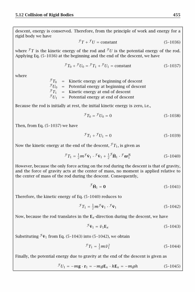
5.12 Collision of Rigid Bodies 455
descent, energy is conserved. Therefore, from the principle of work and energy for arigid body we have
FT + FU = constant (5–1036)
where FT is the kinetic energy of the rod and FU is the potential energy of the rod.Applying Eq. (5–1036) at the beginning and the end of the descent, we have
FT0 + FU0 = FT1 + FU1 = constant (5–1037)
whereFT0 = Kinetic energy at beginning of descentFU0 = Potential energy at beginning of descentFT1 = Kinetic energy at end of descentFU1 = Potential energy at end of descent
Because the rod is initially at rest, the initial kinetic energy is zero, i.e.,
FT0 = FU0 = 0 (5–1038)
Then, from Eq. (5–1037) we have
FT1 + FU1 = 0 (5–1039)
Now the kinetic energy at the end of the descent, FT1, is given as
FT1 = 12m
Fv1 · Fv1 + 12F
H1 · FωR1 (5–1040)
However, because the only force acting on the rod during the descent is that of gravity,and the force of gravity acts at the center of mass, no moment is applied relative tothe center of mass of the rod during the descent. Consequently,
FH1 = 0 (5–1041)
Therefore, the kinetic energy of Eq. (5–1040) reduces to
FT1 = 12m
Fv1 · Fv1 (5–1042)
Now, because the rod translates in the Ex-direction during the descent, we have
Fv1 = v1Ex (5–1043)
Substituting Fv1 from Eq. (5–1043) into (5–1042), we obtain
FT1 = 12mv
21 (5–1044)
Finally, the potential energy due to gravity at the end of the descent is given as
FU1 = −mg · r1 = −mgEx · hEx = −mgh (5–1045)
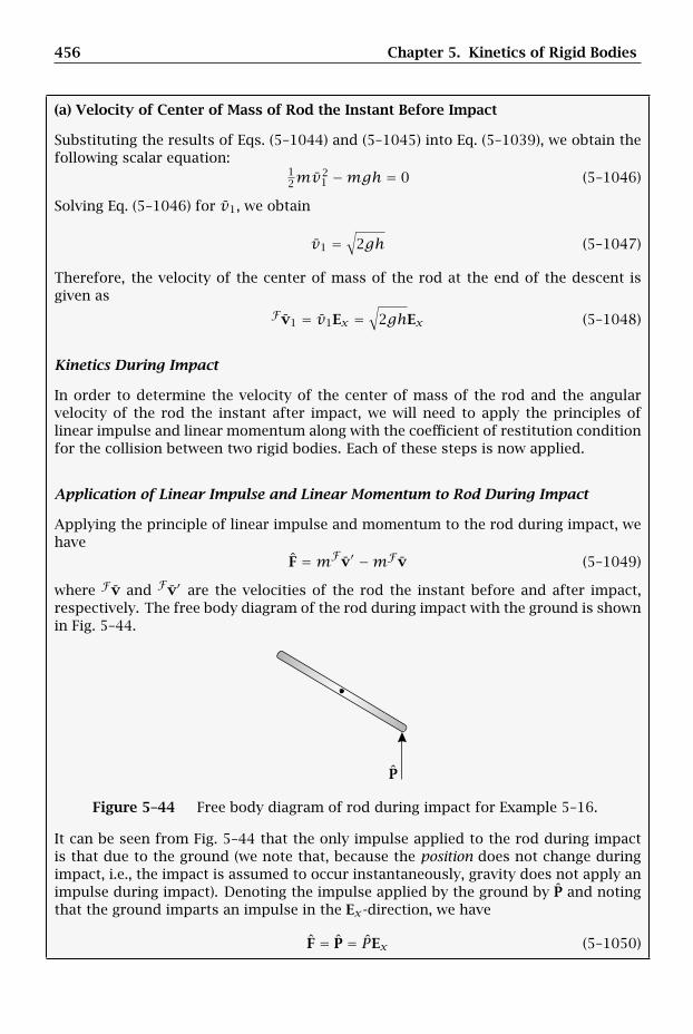
456 Chapter 5. Kinetics of Rigid Bodies
(a) Velocity of Center of Mass of Rod the Instant Before Impact
Substituting the results of Eqs. (5–1044) and (5–1045) into Eq. (5–1039), we obtain thefollowing scalar equation:
12mv
21 −mgh = 0 (5–1046)
Solving Eq. (5–1046) for v1, we obtain
v1 =√
2gh (5–1047)
Therefore, the velocity of the center of mass of the rod at the end of the descent isgiven as
Fv1 = v1Ex =√
2ghEx (5–1048)
Kinetics During Impact
In order to determine the velocity of the center of mass of the rod and the angularvelocity of the rod the instant after impact, we will need to apply the principles oflinear impulse and linear momentum along with the coefficient of restitution conditionfor the collision between two rigid bodies. Each of these steps is now applied.
Application of Linear Impulse and Linear Momentum to Rod During Impact
Applying the principle of linear impulse and momentum to the rod during impact, wehave
F =mFv′ −mFv (5–1049)
where Fv and Fv′ are the velocities of the rod the instant before and after impact,respectively. The free body diagram of the rod during impact with the ground is shownin Fig. 5–44.
P
Figure 5–44 Free body diagram of rod during impact for Example 5–16.
It can be seen from Fig. 5–44 that the only impulse applied to the rod during impactis that due to the ground (we note that, because the position does not change duringimpact, i.e., the impact is assumed to occur instantaneously, gravity does not apply animpulse during impact). Denoting the impulse applied by the ground by P and notingthat the ground imparts an impulse in the Ex-direction, we have
F = P = PEx (5–1050)
5.12 Collision of Rigid Bodies 457
Next, because the impact occurs at the same instant of time as the rod terminates itsdescent, we know that Fv is equal to Fv1 as given in Eq. (5–1048), i.e.,
Fv = Fv1 = v1Ex =√
2ghEx (5–1051)
Finally, using the general expression for the velocity of the center of mass of the rodas given in Eq. (5–1030), the velocity of the center of mass of the rod the instant afterimpact is given as
Fv′1 = v′xEx + v′yEy (5–1052)
Substituting F, Fv, and Fv′ from Eqs. (5–1050), (5–1051), and (5–1052), respectively,into Eq. (5–1049), we obtain
PEx =m(v′xEx + v′yEy)−mv1Ex (5–1053)
Equating components in Eq. (5–1053), we obtain the following two scalar equations:
mv′x −mv1 = P (5–1054)
mv′y = 0 (5–1055)
It is seen from Eq. (5–1055) thatv′y = 0 (5–1056)
Application of Angular Impulse and Angular Momentum to Rod During Impact
Applying the principle of angular impulse and angular momentum to the rod duringimpact relative to the center of mass of the rod, we have
ˆM = FH′ − F
H (5–1057)
whereF
H = Angular momentum of rod relative to center ofmass of rod the instant before impact
FH′ = Angular momentum of rod relative to center of
mass of rod the instant after impact
Because before impact the rod is not rotating, we have
FH = 0 (5–1058)
Next,F
H′ is given asF
H′ = I ·(FωR
1
)′(5–1059)
Because Ex,Ey,Ez is a principal-axis basis, we have
I = IxxEx ⊗ Ex + IyyEy ⊗ Ey + IzzEz ⊗ Ez (5–1060)
Therefore, we obtainF
H′ = Izzω′Ez (5–1061)
458 Chapter 5. Kinetics of Rigid Bodies
Noting that Izz =ml2/12, we obtainF
H′ as
FH′ = ml
2
12ω′Ez (5–1062)
Furthermore, because the only impulse applied to the rod during impact is that due tothe ground, the angular impulse about the center of mass of the rod during impact isgiven as
ˆM = (rB − r)× F = (rB − r)× P (5–1063)
Then, substituting the expression for rB − r from Eq. (5–1034) and the expression forF from Eq. (5–1050) into (5–1063), we have
ˆM =(l2
sinθEx + l2 cosθEy
)× PEx = − l2 P cosθEz (5–1064)
Finally, substitutingF
H′ and ˆM from Eqs. (5–1059) and (5–1064), respectively, into(5–1057), we obtain
− l2P cosθEz = ml
2
12ω′
1Ez (5–1065)
Simplifying Eq. (5–1065 givesml6ω′
1 = −P cosθ (5–1066)
Application of Coefficient of Restitution Condition to Rod During Impact
It is seen that Eqs. (5–1054) and (5–1066) together form a system of two equations inthree unknowns v′x , ω′, and P . Consequently, it is necessary that we obtain anotherindependent equation in order to solve the problem. This last equation is obtained byapplying the coefficient of restitution condition at the impact point B, i.e., applying
e =(FvRB
)′ · n−(FvGB
)′ · n
FvGB · n− FvRB · n(5–1067)
where the superscript G denotes the fixed horizontal surface and n is the direction ofimpact. Since the horizontal surface is fixed, we have(
FvGB)′ = FvGB = 0 (5–1068)
Furthermore, since the impact occurs in the Ex-direction, the direction of impact, n, isgiven as
n = Ex (5–1069)
Therefore, Eq. (5–1067) reduces to
e = −(FvRB
)′ · ExFvRB · Ex
(5–1070)
which can be rearranged to give(FvRB
)′ · Ex = −eFvRB · Ex (5–1071)
5.12 Collision of Rigid Bodies 459
Now, Eq. (5–1071) can be resolved in terms of components using the expression forFvB as given in Eq. (5–1035). First, because the rod is not rotating before impact, wehave
FvB = Fv = v1Ex = vEx =√
2ghEx (5–1072)
Next, using Eq. (5–1035), the velocity of point B in reference frame F the instant afterimpact is given as
(FvRB
)′ = (v′x −
lω′
2cosθ
)Ex +
(v′y +
lω′
2sinθ
)Ey (5–1073)
Substituting the expressions for FvRB and(FvRB
)′from Eqs. (5–1072) and (5–1073) into
Eq. (5–1071), we obtain
v′x −l2ω′ cosθ = −ev (5–1074)
(b) Angular Velocity and Velocity of Center of Mass of Rod the Instant After Impact
Equations (5–1054), (5–1066), and (5–1074) are a system of three equations in the threeunknowns v2x , ω2, and P . Multiplying Eq. (5–1054) by cosθ , we obtain
mv′x cosθ −mv cosθ = P cosθ (5–1075)
Adding Eq. (5–1075) to (5–1066), we have
mv′x cosθ −mv cosθ + ml6ω′ = 0 (5–1076)
Dropping the dependence on m in Eq. (5–1076) gives
v′x cosθ − v cosθ + l6ω′ = 0 (5–1077)
Next, multiplying Eq. (5–1074) by cosθ gives
v′x cosθ − l2ω′ cos2θ = −ev cosθ (5–1078)
Subtracting Eq. (5–1078) from (5–1077) gives
−v cosθ + l6ω′ + l
2ω′ cos2θ = ev cosθ (5–1079)
Rearranging Eq. (5–1079) gives
lω′(
16+ 1
2cos2θ
)= (1+ e)v cosθ (5–1080)
Solving Eq. (5–1080) for ω2 gives
ω′ = 6(1+ e) cosθl(1+ 3 cos2θ)
v (5–1081)
460 Chapter 5. Kinetics of Rigid Bodies
Recalling from Eq. (5–1047) that v = √2gh, we obtain the angular velocity of the rod
immediately after impact as
(FωR
)′ = 6(1+ e) cosθl(1+ 3 cos2θ)
√2ghEz (5–1082)
Substituting ω2 from Eq. (5–1082) into (5–1077) gives
v′x cosθ − v cosθ + l6
6(1+ e) cosθl(1+ 3 cos2θ)
v = 0 (5–1083)
Solving Eq. (5–1083) for v′x gives
v′x = v −1+ e
1+ 3 cos2θv (5–1084)
Equation (5–1084) can be simplified to
v′x =3 cos2θ − e1+ 3 cos2θ
v (5–1085)
Recalling from Eq. (5–1047) that v = √2gh, we obtain
v′x =3 cos2θ − e1+ 3 cos2θ
√2gh (5–1086)
We then obtain the post-impact velocity of the center of mass after impact as
Fv′ = 3 cos2θ − e1+ 3 cos2θ
√2ghEx (5–1087)
Example 5–17
A uniform slender rod of mass M and length L is hinged at point O, located at one ofits ends as shown in Fig. 5–45. The rod is initially at rest when it is struck by a particleof mass m traveling with a horizontal velocity of v0. Assuming a perfectly inelasticimpact, determine (a) the distance x (measured from point O) at which the particlemust strike the rod in order that the reaction impulse at the pivot is zero and (b) theangular velocity of the rod immediately after impact.
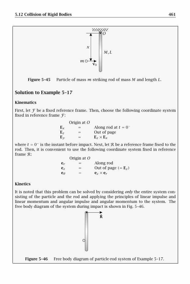
5.12 Collision of Rigid Bodies 461
v0
M,L
m
x
O
Figure 5–45 Particle of mass m striking rod of mass M and length L.
Solution to Example 5–17
Kinematics
First, let F be a fixed reference frame. Then, choose the following coordinate systemfixed in reference frame F :
Origin at OEx = Along rod at t = 0−
Ez = Out of pageEy = Ez × Ex
where t = 0− is the instant before impact. Next, let R be a reference frame fixed to therod. Then, it is convenient to use the following coordinate system fixed in referenceframe R:
Origin at Oer = Along rodez = Out of page (= Ez)eθ = ez × er
Kinetics
It is noted that this problem can be solved by considering only the entire system con-sisting of the particle and the rod and applying the principles of linear impulse andlinear momentum and angular impulse and angular momentum to the system. Thefree body diagram of the system during impact is shown in Fig. 5–46.
R
Figure 5–46 Free body diagram of particle-rod system of Example 5–17.

462 Chapter 5. Kinetics of Rigid Bodies
Examining Fig. 5–46, it can be seen that the only impulse applied to the system duringimpact is the reaction impulse R that acts at the location of the hinge at point O. Wenow apply the principles of linear impulse and linear momentum and angular impulseand angular momentum to the system during impact.
Application of Linear Impulse and Momentum to System
Applying the principle of linear impulse and momentum to the entire system, we have
FG′ − FG = F (5–1088)
where FG and FG′ are the linear momenta of the system before and after impact,respectively. Now, because the rod is initially motionless, the linear momentum of thesystem before impact is due entirely to the particle, which implies that
FG =mFvp (5–1089)
where Fvp is the velocity of the particle in reference frame F before impact. Further-more, the linear momentum of the system after impact is due to motion of both therod and the particle, which implies that
FG′ = FG′p + FG′r (5–1090)
where FG′p and FG′r are the linear momenta of the particle and rod, respectively, afterimpact. The linear momentum of the particle after impact is given as
FG′p =mFv′p (5–1091)
where Fv′p is the velocity of the particle after impact. Next, the linear momentum ofthe rod after impact is given as
FG′r = MFv′r (5–1092)
where Fv′r is the velocity of the center of mass of the rod after impact. Adding theexpressions in Eqs. (5–1091) and (5–1092), we obtain the post-impact linear momentumof the system as
FG′ =mFv′p +MFv′r (5–1093)
Substituting the results of Eqs. (5–1089) and (5–1093) into Eq. (5–1088), we obtain
mFv′p +MFv′r −mFvp = F (5–1094)
Now, we are given the initial velocity of the particle as
Fvp = v0eθ (5–1095)
Furthermore, denoting the angular velocity of the rod immediately after impact by(FωR)′, from kinematics we have
Fv′r =(Fdrdt
)′=(Rdrdt+ FωR × r
)′(5–1096)
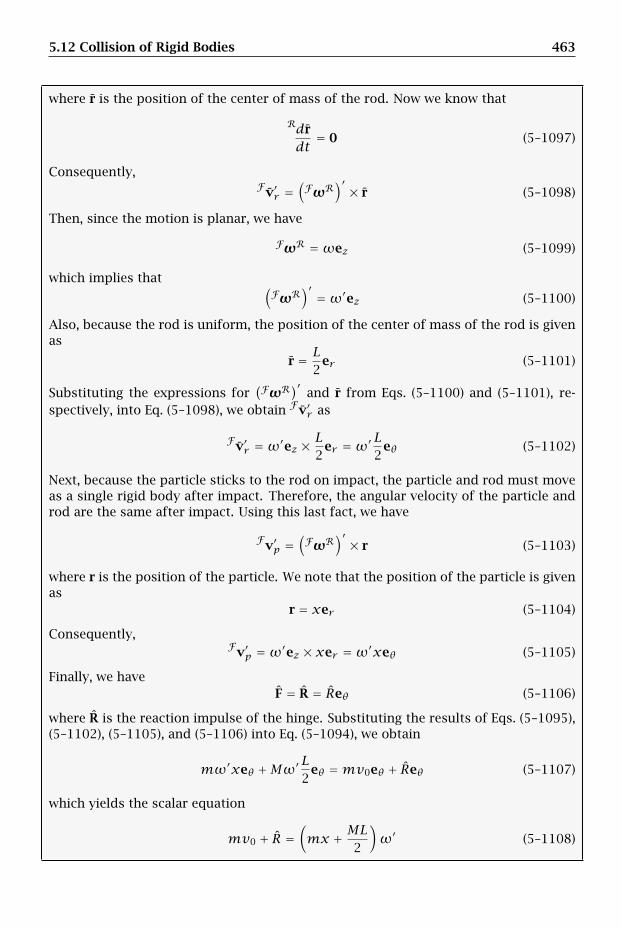
5.12 Collision of Rigid Bodies 463
where r is the position of the center of mass of the rod. Now we know that
Rdrdt
= 0 (5–1097)
Consequently,Fv′r =
(FωR
)′ × r (5–1098)
Then, since the motion is planar, we have
FωR =ωez (5–1099)
which implies that (FωR
)′ =ω′ez (5–1100)
Also, because the rod is uniform, the position of the center of mass of the rod is givenas
r = L2
er (5–1101)
Substituting the expressions for(FωR)′ and r from Eqs. (5–1100) and (5–1101), re-
spectively, into Eq. (5–1098), we obtain Fv′r as
Fv′r =ω′ez × L2er =ω′L2
eθ (5–1102)
Next, because the particle sticks to the rod on impact, the particle and rod must moveas a single rigid body after impact. Therefore, the angular velocity of the particle androd are the same after impact. Using this last fact, we have
Fv′p =(FωR
)′ × r (5–1103)
where r is the position of the particle. We note that the position of the particle is givenas
r = xer (5–1104)
Consequently,Fv′p =ω′ez × xer =ω′xeθ (5–1105)
Finally, we haveF = R = Reθ (5–1106)
where R is the reaction impulse of the hinge. Substituting the results of Eqs. (5–1095),(5–1102), (5–1105), and (5–1106) into Eq. (5–1094), we obtain
mω′xeθ +Mω′L2
eθ =mv0eθ + Reθ (5–1107)
which yields the scalar equation
mv0 + R =(mx + ML
2
)ω′ (5–1108)
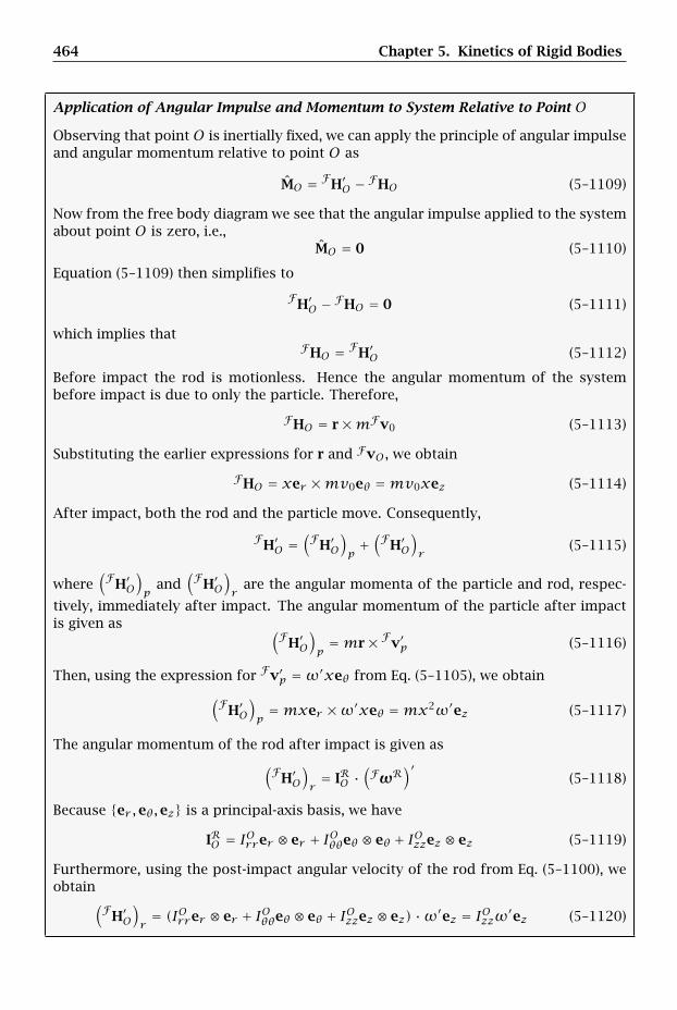
464 Chapter 5. Kinetics of Rigid Bodies
Application of Angular Impulse and Momentum to System Relative to Point O
Observing that point O is inertially fixed, we can apply the principle of angular impulseand angular momentum relative to point O as
MO = FH′O − FHO (5–1109)
Now from the free body diagram we see that the angular impulse applied to the systemabout point O is zero, i.e.,
MO = 0 (5–1110)
Equation (5–1109) then simplifies to
FH′O − FHO = 0 (5–1111)
which implies thatFHO = FH′O (5–1112)
Before impact the rod is motionless. Hence the angular momentum of the systembefore impact is due to only the particle. Therefore,
FHO = r×mFv0 (5–1113)
Substituting the earlier expressions for r and FvO , we obtain
FHO = xer ×mv0eθ =mv0xez (5–1114)
After impact, both the rod and the particle move. Consequently,
FH′O =(FH′O
)p+(FH′O
)r
(5–1115)
where(FH′O
)p
and(FH′O
)r
are the angular momenta of the particle and rod, respec-
tively, immediately after impact. The angular momentum of the particle after impactis given as (FH′O
)p=mr× Fv′p (5–1116)
Then, using the expression for Fv′p =ω′xeθ from Eq. (5–1105), we obtain(FH′O
)p=mxer ×ω′xeθ =mx2ω′ez (5–1117)
The angular momentum of the rod after impact is given as(FH′O)r= IRO ·
(FωR
)′(5–1118)
Because er ,eθ,ez is a principal-axis basis, we have
IRO = IOrrer ⊗ er + IOθθeθ ⊗ eθ + IOzzez ⊗ ez (5–1119)
Furthermore, using the post-impact angular velocity of the rod from Eq. (5–1100), weobtain(FH′O
)r= (IOrrer ⊗ er + IOθθeθ ⊗ eθ + IOzzez ⊗ ez) ·ω′ez = IOzzω′ez (5–1120)
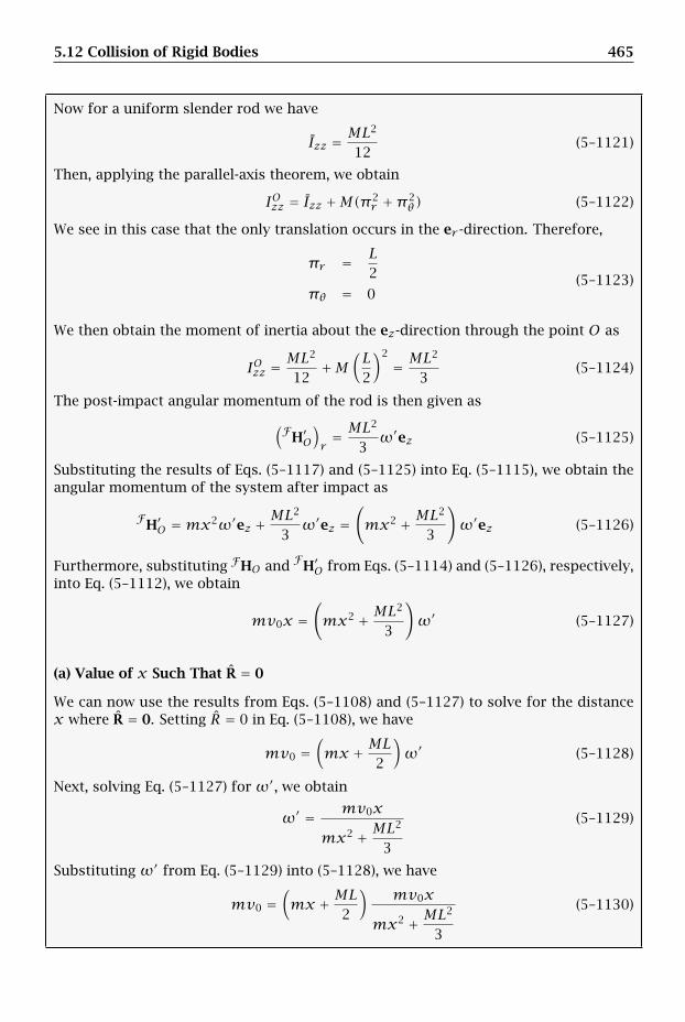
5.12 Collision of Rigid Bodies 465
Now for a uniform slender rod we have
Izz = ML2
12(5–1121)
Then, applying the parallel-axis theorem, we obtain
IOzz = Izz +M(π2r +π2
θ) (5–1122)
We see in this case that the only translation occurs in the er -direction. Therefore,
πr = L2
πθ = 0(5–1123)
We then obtain the moment of inertia about the ez-direction through the point O as
IOzz =ML2
12+M
(L2
)2
= ML2
3(5–1124)
The post-impact angular momentum of the rod is then given as
(FH′O)r= ML
2
3ω′ez (5–1125)
Substituting the results of Eqs. (5–1117) and (5–1125) into Eq. (5–1115), we obtain theangular momentum of the system after impact as
FH′O =mx2ω′ez + ML2
3ω′ez =
(mx2 + ML
2
3
)ω′ez (5–1126)
Furthermore, substituting FHO and FH′O from Eqs. (5–1114) and (5–1126), respectively,into Eq. (5–1112), we obtain
mv0x =(mx2 + ML
2
3
)ω′ (5–1127)
(a) Value of x Such That R = 0
We can now use the results from Eqs. (5–1108) and (5–1127) to solve for the distancex where R = 0. Setting R = 0 in Eq. (5–1108), we have
mv0 =(mx + ML
2
)ω′ (5–1128)
Next, solving Eq. (5–1127) for ω′, we obtain
ω′ = mv0x
mx2 + ML2
3
(5–1129)
Substituting ω′ from Eq. (5–1129) into (5–1128), we have
mv0 =(mx + ML
2
)mv0x
mx2 + ML2
3
(5–1130)
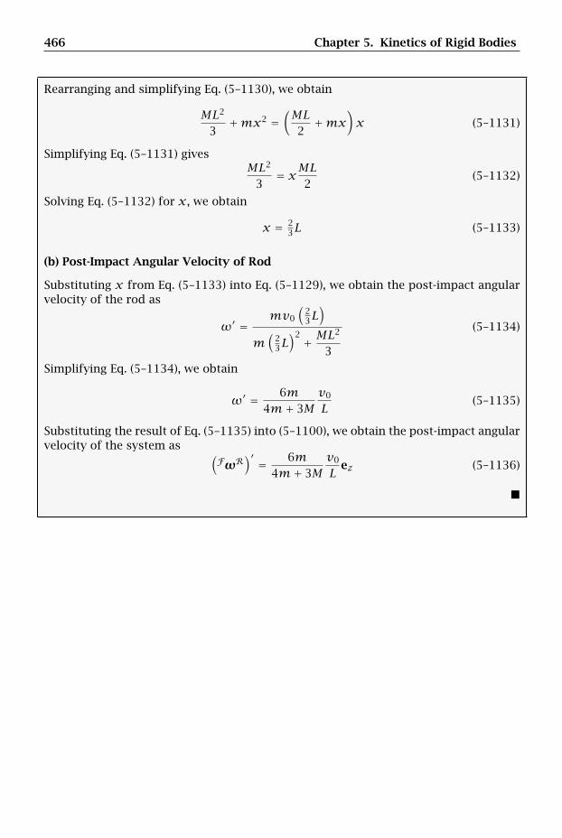
466 Chapter 5. Kinetics of Rigid Bodies
Rearranging and simplifying Eq. (5–1130), we obtain
ML2
3+mx2 =
(ML2+mx
)x (5–1131)
Simplifying Eq. (5–1131) givesML2
3= xML
2(5–1132)
Solving Eq. (5–1132) for x, we obtain
x = 23L (5–1133)
(b) Post-Impact Angular Velocity of Rod
Substituting x from Eq. (5–1133) into Eq. (5–1129), we obtain the post-impact angularvelocity of the rod as
ω′ =mv0
(23L)
m(
23L)2 + ML
2
3
(5–1134)
Simplifying Eq. (5–1134), we obtain
ω′ = 6m4m+ 3M
v0
L(5–1135)
Substituting the result of Eq. (5–1135) into (5–1100), we obtain the post-impact angularvelocity of the system as (
FωR)′ = 6m
4m+ 3Mv0
Lez (5–1136)
Summary of Chapter 5 467
Summary of Chapter 5
This chapter was devoted to developing the framework for solving and analyzing rigidbody kinetics problems. The first topics covered were the center of mass and linearmomentum of a rigid body. The position of the center of mass of a rigid body wasdefined as
r =
∫R
rdm
m(5–1)
where r is measured relative point O fixed in an inertial reference frame N . In termsof the center of mass, the linear momentum of a rigid body was derived as
NG =mNv (5–9)
where NvNv =
Ndrdt
(5–10)
is the velocity of the center of mass of the rigid body in the inertial reference frameN .Finally, the acceleration of the center of mass of a rigid body as viewed by an observerin an inertial reference frame N was given as
Na =Nddt
(Nv
)
The next topic covered in this chapter was the angular momentum of a rigid body.The angular momentum of a rigid body in an inertial reference frame N relative to anarbitrary reference point Q was defined as
NHQ =∫R(r− rQ)× (Nv−NvQ)dm (5–13)
The angular momentum of a rigid body in the inertial reference frame N relative to apoint O fixed in N was defined as
NHO =∫R(r− rO)×Nvdm (5–14)
The angular momentum of a rigid body in the inertial reference frame N relative tothe center of mass of the rigid body was defined as
NH =
∫R(r− r)× (Nv−Nv)dm (5–15)
Using the three definitions of angular momentum, it was shown that NHQ and NHOare related as
NHQ = NHO − (r− rQ)×mNvQ − (rQ − rO)×mNv (5–21)
Next, it was shown thatN
H and NHO are related as
NH = NHO − (r− rO)×mNv (5–22)
468 Chapter 5. Kinetics of Rigid Bodies
Finally, it was shown that NHQ andN
H are related as
NHQ = NH+ (rQ − r)×m(NvQ −Nv) (5–24)
The next topic that was covered in this chapter was the derivation of the angularmomentum of a rigid body in terms of the moment of inertia tensor. The moment ofinertia tensor relative to a body-fixed point Q was derived as
IRQ =∫R
[(ρQ · ρQ
)U−
(ρQ ⊗ ρQ
)]dm (5–36)
It was then shown that the angular momentum of a rigid body R relative to a body-fixed point Q can be written as
NHQ = IRQ · NωR (5–39)
where ρQ = r− rQ. Next, it was shown that the moment of inertia tensor relative to thecenter of mass of a rigid body can be written as
IR =
∫R[(ρ · ρ)U− (ρ⊗ ρ)]dm (5–43)
where ρ = r − r. It was then shown that the angular momentum of a rigid body Rrelative to the center of mass of a rigid body is given as
NH = I
R · NωR (5–44)
Then, for a body-fixed coordinate system with origin at the body-fixed point Q, themoments of inertia of the rigid body were derived as
IQ11 =∫R(ρ2
2 + ρ23)dm
IQ22 =∫R(ρ2
1 + ρ23)dm
IQ33 =∫R(ρ2
1 + ρ22)dm
(5–54)
Similarly, the products of inertia relative to the body-fixed point Q were derived as
IQ12 = −∫Rρ1ρ2dm
IQ13 = −∫Rρ1ρ3dm
IQ23 = −∫Rρ2ρ3dm
(5–55)
For the case where the reference point is the center of mass, the moments of inertiawere derived as
I11 =∫R(ρ2
2 + ρ23)dm
I22 =∫R(ρ2
1 + ρ23)dm
I33 =∫R(ρ2
1 + ρ22)dm
(5–56)
Summary of Chapter 5 469
Furthermore, the products of inertia relative to the center of mass of the rigid bodywere derived as
I12 = −∫Rρ1ρ2dm
I13 = −∫Rρ1ρ3dm
I23 = −∫Rρ2ρ3dm
(5–57)
After defining the moments and products of inertia for a rigid body, it was shown thatthe moments and products of inertia relative to a body-fixed point Q are related tothe moments and products of inertia relative to the center of mass via the parallel-axistheorem as
IQ11 = I11 +m(π22 +π2
3 )
IQ22 = I22 +m(π21 +π2
3 )
IQ33 = I33 +m(π21 +π2
2 )
IQ12 = IQ21 = I12 −mπ1π2
IQ13 = IQ31 = I13 −mπ1π3
IQ23 = IQ32 = I23 −mπ2π3
(5–78)
where π = rQ − r = π1e1 + π2e2 + π3e3. Finally, it was discussed that, for the case
of a principal-axis coordinate system, the products of inertia are zero, i.e., IQij = 0 (i ≠j, i, j = 1,2,3)
The next topics covered were Euler’s laws for a rigid body. Euler’s laws were statedas follows:
F =mNa (5–225)
and
MO =Nddt
(NHO
)(5–226)
where O is a point fixed point in an inertial reference frame N . It was then shownthat, for an arbitrary reference point Q, Euler’s 2nd law is given as
MQ − (r− rQ)×mNaQ =Nddt
(NHQ
)(5–235)
Finally, for the case where the reference point is the center of mass of the rigid body,it was shown that
M =Nddt
(NH)
(5–237)
In terms of the moment of inertia tensor relative to a point Q fixed in the rigid body,it was shown that Euler’s 2nd law can be written as
MQ − (r− rQ)×mNaQ = IRQ · NαR +NωR ×(IRQ · NωR
)(5–681)
Similarly, in terms of the moment of inertia tensor relative to the center of mass of therigid body, it was shown that Euler’s 2nd law can be written as
M = IR · NαR +NωR ×
(IR · NωR
)(5–683)
470 Chapter 5. Kinetics of Rigid Bodies
Finally, in terms of a body-fixed principal-axis coordinate system located at the centerof mass of the rigid body, it was shown that Eq. (5–683) leads to the following threescalar equations:
M1 = I1ω1 + (I3 − I2)ω3ω2 (5–701)
M2 = I2ω2 + (I1 − I3)ω1ω3 (5–702)
M3 = I3ω3 + (I2 − I1)ω2ω1 (5–703)
It was stated that Eqs. (5–701)–(5–703) are called Euler’s equations for a rigid body.The next topics covered were power, work, and energy of a rigid body. The kinetic
energy of a rigid body as viewed by an observer in an inertial reference frame N wasdefined as
NT = 12
∫RNv · Nvdm (5–767)
A more useful expression for the kinetic energy of a rigid body, called Koenig’s decom-position, was derived as
NT = 12m
Nv · Nv+ 12N
H · NωR (5–786)
The work-energy theorem for a rigid body was then derived as
ddt
(NT
)= F · Nv+ M · NωR (5–799)
A more useful form of the work-energy theorem for a rigid body was then derived as
ddt
(NT
)=
n∑i=1
Fi · Nvi + τ · NωR (5–809)
Using the work-energy theorem for a rigid body, the principle of work and energy fora rigid body was derived as
NT2 −NT1 = NWF12 +NWτ
12 (5–814)
whereNWF
12 is the work done by all of the forces acting on the body while NWτ12
is the work done by all of the pure torques acting on the body over a time intervalt ∈ [t1, t2]. Then, using the work-energy theorem and the concept of a conservativeforce, an alternate form of the work-energy theorem was derived as
ddt
(NE
)=
q∑i=1
Fnci · Nvnci + τnc · NωR (5–823)
where q is the number of nonconservative forces acting on the rigid body. Finally,using the alternate form of the work-energy theorem for a rigid body, the alternateform of the principle of work and energy for a rigid body was derived as
NE2 −NE1 = NWFnc12 +NWτnc
12 (5–831)
where NWFnc12 is the work done by all of the nonconservative forces acting on the body
while NWτnc12 is the work done by all of the nonconservative pure torques acting on the
body over a time interval t ∈ [t1, t2].
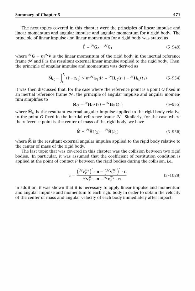
Summary of Chapter 5 471
The next topics covered in this chapter were the principles of linear impulse andlinear momentum and angular impulse and angular momentum for a rigid body. Theprinciple of linear impulse and linear momentum for a rigid body was stated as
F = NG2 −NG1 (5–949)
where NG = mNv is the linear momentum of the rigid body in the inertial referenceframeN and F is the resultant external linear impulse applied to the rigid body. Then,the principle of angular impulse and momentum was derived as
MQ −∫ t2t1(r− rQ)×mNaQdt = NHQ(t2)−NHQ(t1) (5–954)
It was then discussed that, for the case where the reference point is a point O fixed inan inertial reference frame N , the principle of angular impulse and angular momen-tum simplifies to
MO = NHO(t2)−NHO(t1) (5–955)
where MO is the resultant external angular impulse applied to the rigid body relativeto the point O fixed in the inertial reference frame N . Similarly, for the case wherethe reference point is the center of mass of the rigid body, we have
ˆM = NH(t2)−N
H(t1) (5–956)
where ˆM is the resultant external angular impulse applied to the rigid body relative tothe center of mass of the rigid body.
The last topic that was covered in this chapter was the collision between two rigidbodies. In particular, it was assumed that the coefficient of restitution condition isapplied at the point of contact P between the rigid bodies during the collision, i.e.,
e =(NvR2
P
)′ · n−(NvR1
P
)′ · n
NvR1P · n−NvR2
P · n(5–1029)
In addition, it was shown that it is necessary to apply linear impulse and momentumand angular impulse and momentum to each rigid body in order to obtain the velocityof the center of mass and angular velocity of each body immediately after impact.
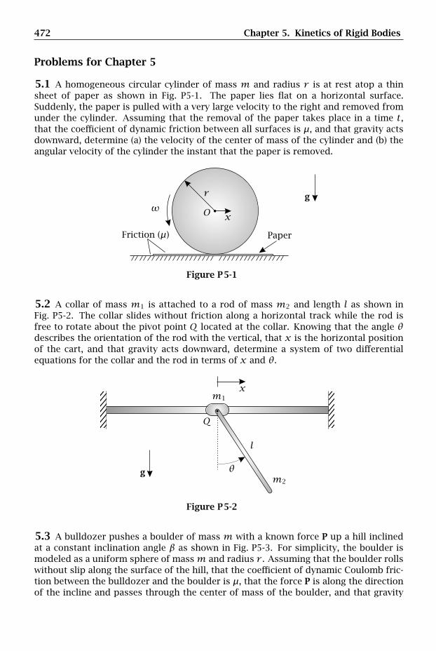
472 Chapter 5. Kinetics of Rigid Bodies
Problems for Chapter 5
5.1 A homogeneous circular cylinder of mass m and radius r is at rest atop a thinsheet of paper as shown in Fig. P5-1. The paper lies flat on a horizontal surface.Suddenly, the paper is pulled with a very large velocity to the right and removed fromunder the cylinder. Assuming that the removal of the paper takes place in a time t,that the coefficient of dynamic friction between all surfaces is µ, and that gravity actsdownward, determine (a) the velocity of the center of mass of the cylinder and (b) theangular velocity of the cylinder the instant that the paper is removed.
Friction (µ) Paper
gr
xOω
Figure P5-1
5.2 A collar of mass m1 is attached to a rod of mass m2 and length l as shown inFig. P5-2. The collar slides without friction along a horizontal track while the rod isfree to rotate about the pivot point Q located at the collar. Knowing that the angle θdescribes the orientation of the rod with the vertical, that x is the horizontal positionof the cart, and that gravity acts downward, determine a system of two differentialequations for the collar and the rod in terms of x and θ.
g
l
m1
m2
x
Q
θ
Figure P5-2
5.3 A bulldozer pushes a boulder of mass m with a known force P up a hill inclinedat a constant inclination angle β as shown in Fig. P5-3. For simplicity, the boulder ismodeled as a uniform sphere of massm and radius r . Assuming that the boulder rollswithout slip along the surface of the hill, that the coefficient of dynamic Coulomb fric-tion between the bulldozer and the boulder is µ, that the force P is along the directionof the incline and passes through the center of mass of the boulder, and that gravity
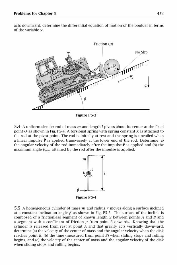
Problems for Chapter 5 473
acts downward, determine the differential equation of motion of the boulder in termsof the variable x.
Friction (µ)
No Slip
P
g
r
x
O
β
Figure P5-3
5.4 A uniform slender rod of massm and length l pivots about its center at the fixedpoint O as shown in Fig. P5-4. A torsional spring with spring constant K is attached tothe rod at the pivot point. The rod is initially at rest and the spring is uncoiled whena linear impulse P is applied transversely at the lower end of the rod. Determine (a)the angular velocity of the rod immediately after the impulse P is applied and (b) themaximum angle θmax attained by the rod after the impulse is applied.
P
l
m
KO
Figure P5-4
5.5 A homogeneous cylinder of mass m and radius r moves along a surface inclinedat a constant inclination angle β as shown in Fig. P5-5. The surface of the incline iscomposed of a frictionless segment of known length x between points A and B anda segment with a coefficient of friction µ from point B onwards. Knowing that thecylinder is released from rest at point A and that gravity acts vertically downward,determine (a) the velocity of the center of mass and the angular velocity when the diskreaches point B, (b) the time (measured from point B) when sliding stops and rollingbegins, and (c) the velocity of the center of mass and the angular velocity of the diskwhen sliding stops and rolling begins.
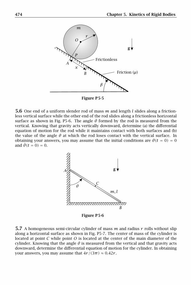
474 Chapter 5. Kinetics of Rigid Bodies
Frictionless
Friction (µ)
g
m
r
xA
B
O
P
β
Figure P5-5
5.6 One end of a uniform slender rod of mass m and length l slides along a friction-less vertical surface while the other end of the rod slides along a frictionless horizontalsurface as shown in Fig. P5-6. The angle θ formed by the rod is measured from thevertical. Knowing that gravity acts vertically downward, determine (a) the differentialequation of motion for the rod while it maintains contact with both surfaces and (b)the value of the angle θ at which the rod loses contact with the vertical surface. Inobtaining your answers, you may assume that the initial conditions are θ(t = 0) = 0and θ(t = 0) = 0.
g
m, l
A
B
Cθ
Figure P5-6
5.7 A homogeneous semi-circular cylinder of mass m and radius r rolls without slipalong a horizontal surface as shown in Fig. P5-7. The center of mass of the cylinder islocated at point C while point O is located at the center of the main diameter of thecylinder. Knowing that the angle θ is measured from the vertical and that gravity actsdownward, determine the differential equation of motion for the cylinder. In obtainingyour answers, you may assume that 4r/(3π) ≈ 0.42r .
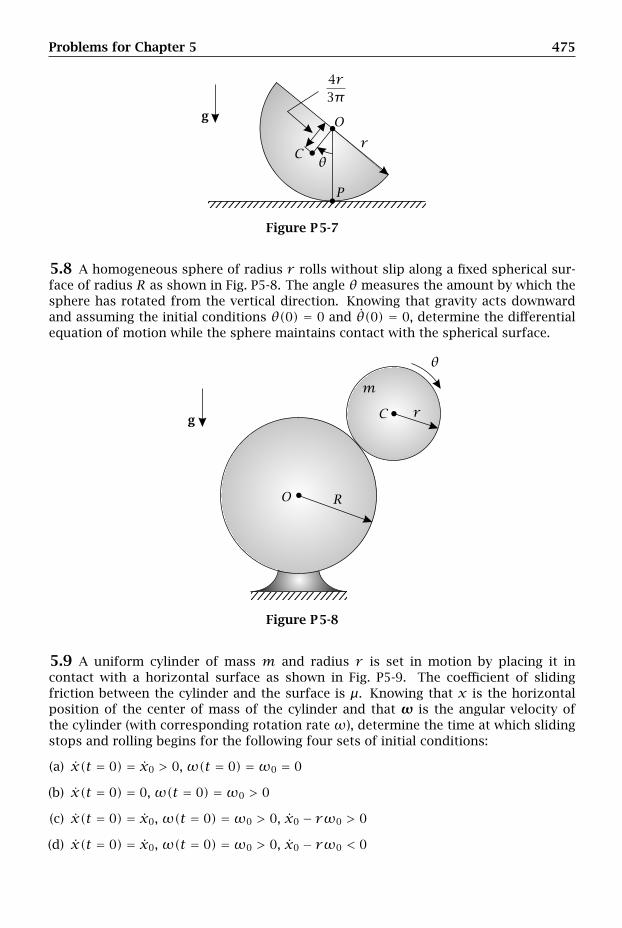
Problems for Chapter 5 475
g
rC
O
P
4r3π
θ
Figure P5-7
5.8 A homogeneous sphere of radius r rolls without slip along a fixed spherical sur-face of radius R as shown in Fig. P5-8. The angle θ measures the amount by which thesphere has rotated from the vertical direction. Knowing that gravity acts downwardand assuming the initial conditions θ(0) = 0 and θ(0) = 0, determine the differentialequation of motion while the sphere maintains contact with the spherical surface.
g
m
rC
O R
θ
Figure P5-8
5.9 A uniform cylinder of mass m and radius r is set in motion by placing it incontact with a horizontal surface as shown in Fig. P5-9. The coefficient of slidingfriction between the cylinder and the surface is µ. Knowing that x is the horizontalposition of the center of mass of the cylinder and that ω is the angular velocity ofthe cylinder (with corresponding rotation rate ω), determine the time at which slidingstops and rolling begins for the following four sets of initial conditions:
(a) x(t = 0) = x0 > 0, ω(t = 0) =ω0 = 0
(b) x(t = 0) = 0, ω(t = 0) =ω0 > 0
(c) x(t = 0) = x0, ω(t = 0) =ω0 > 0, x0 − rω0 > 0
(d) x(t = 0) = x0, ω(t = 0) =ω0 > 0, x0 − rω0 < 0

476 Chapter 5. Kinetics of Rigid Bodies
Friction (µ)
gr
xO
ω
Figure P5-9
5.10 A uniform circular disk of mass m and radius r rolls without slip along a planeinclined at a constant angle β with horizontal as shown in Fig. P5-10. Attached at thecenter of the disk is a linear spring with spring constant K. Knowing that the spring isunstretched when the angle θ is zero and that gravity acts downward, determine thedifferential equation of motion for the disk in terms of the angle θ.
g
r
K
O
P
β
θ
Figure P5-10
5.11 A uniform circular disk of mass m and radius r is set in motion such that itsinitial angular velocity is ω0 and its initial translational velocity is zero, as shownin Fig. P5-11. The disk is then immediately placed in contact with a surface that isinclined at an angle β with the horizontal. Knowing that the coefficient of slidingCoulomb friction between the disk and the surface is µ and that gravity acts downward,determine (a) the distance traveled by the disk up the incline while the disk is slidingand (b) the duration of time for which the disk slides before rolling begins.
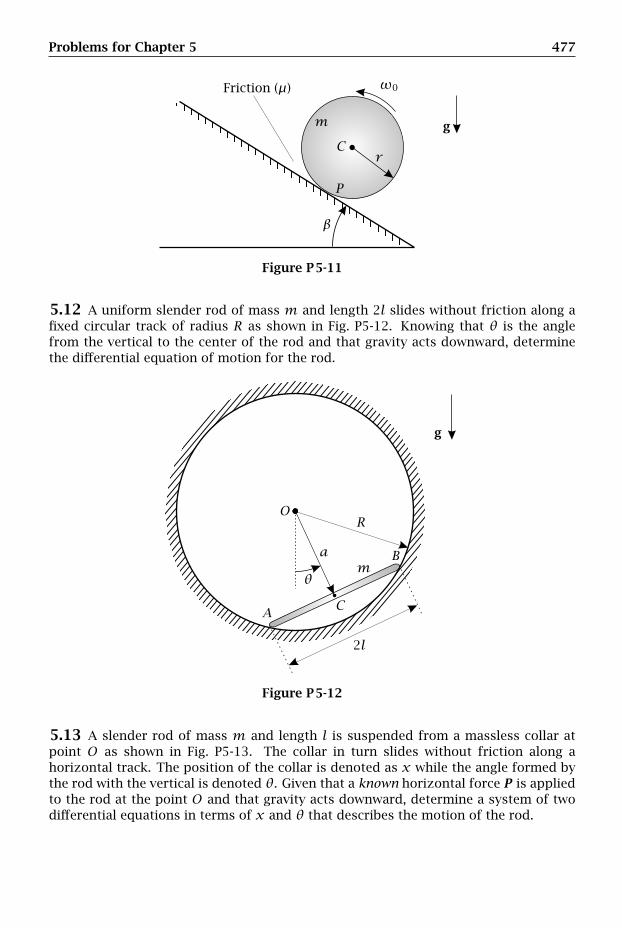
Problems for Chapter 5 477
ω0Friction (µ)
gm
rC
P
β
Figure P5-11
5.12 A uniform slender rod of mass m and length 2l slides without friction along afixed circular track of radius R as shown in Fig. P5-12. Knowing that θ is the anglefrom the vertical to the center of the rod and that gravity acts downward, determinethe differential equation of motion for the rod.
2l
g
am
A
B
C
OR
θ
Figure P5-12
5.13 A slender rod of mass m and length l is suspended from a massless collar atpoint O as shown in Fig. P5-13. The collar in turn slides without friction along ahorizontal track. The position of the collar is denoted as x while the angle formed bythe rod with the vertical is denoted θ. Given that a known horizontal force P is appliedto the rod at the point O and that gravity acts downward, determine a system of twodifferential equations in terms of x and θ that describes the motion of the rod.

478 Chapter 5. Kinetics of Rigid Bodies
x(t)
P
g l
m
O
θ
Figure P5-13
5.14 A uniform slender rod of mass m and length l is translating horizontally witha velocity v0 and is not rotating when it strikes a fixed surface inclined at an angle βwith the horizontal as shown in Fig. P5-14. Assuming that the coefficient of restitutionbetween the rod and the incline is e, determine the following quantities relative to theincline at the instant after the impact has occurred: (a) the velocity of the center ofmass of the rod and (b) the angular velocity of the rod.
v0 A C
β
Figure P5-14
5.15 A system consists of two slender rods, one of massm and length l and the otherof mass m and length 3l, attached to form a double pendulum as shown in Fig. P5-15.The rods are initially motionless when the lower rod is struck by a horizontal impulseP at a distance x from the hinge point connecting the two rods. Assuming no gravity,determine the value of x for which the two rods will rotate with the same angularvelocity (relative to the ground) the instant after the impulse is applied.
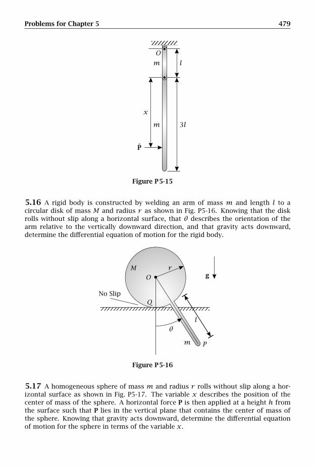
Problems for Chapter 5 479
3l
P
l
m
m
x
O
Figure P5-15
5.16 A rigid body is constructed by welding an arm of mass m and length l to acircular disk of mass M and radius r as shown in Fig. P5-16. Knowing that the diskrolls without slip along a horizontal surface, that θ describes the orientation of thearm relative to the vertically downward direction, and that gravity acts downward,determine the differential equation of motion for the rigid body.
No Slip
g
l
m
rMO
P
Q
θ
Figure P5-16
5.17 A homogeneous sphere of mass m and radius r rolls without slip along a hor-izontal surface as shown in Fig. P5-17. The variable x describes the position of thecenter of mass of the sphere. A horizontal force P is then applied at a height h fromthe surface such that P lies in the vertical plane that contains the center of mass ofthe sphere. Knowing that gravity acts downward, determine the differential equationof motion for the sphere in terms of the variable x.

480 Chapter 5. Kinetics of Rigid Bodies
No Slip
P g
rh
x
O
P
Figure P5-17
5.18 A uniform disk of mass m and radius r rolls without slip along the inside of afixed circular track of radius R as shown in Fig. P5-18. The angles θ and φ measurethe position of the center of the disk and the angle of rotation of the disk, respec-tively, relative to the vertically downward direction. Knowing that the angles θ andφ are simultaneously zero and that gravity acts downward, determine the differentialequation of motion for the disk in terms of the angle θ.
g
m
rC
O
R
θ
φ
Figure P5-18
5.19 A slender uniform rod of massM and length L is hinged at one of its ends at thepoint O as shown in Fig. P5-19. Attached to the rod is a torsional spring with springconstant K and uncoiled angle zero. The rod is initially motionless at the equilibriumposition of the spring when it is struck by a particle of massmmoving with velocity v0
at a horizontal distance x from the hinge point. Assuming no gravity and a perfectly
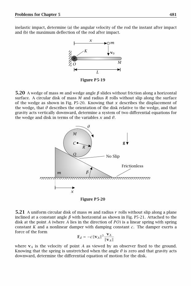
Problems for Chapter 5 481
inelastic impact, determine (a) the angular velocity of the rod the instant after impactand (b) the maximum deflection of the rod after impact.
v0
mx
K
L
MO
Figure P5-19
5.20 A wedge of massm and wedge angle β slides without friction along a horizontalsurface. A circular disk of mass M and radius R rolls without slip along the surfaceof the wedge as shown in Fig. P5-20. Knowing that x describes the displacement ofthe wedge, that θ describes the orientation of the disk relative to the wedge, and thatgravity acts vertically downward, determine a system of two differential equations forthe wedge and disk in terms of the variables x and θ.
Frictionless
No Slip
g
m
x
C
M
Q
R
β
θ
Figure P5-20
5.21 A uniform circular disk of mass m and radius r rolls without slip along a planeinclined at a constant angle β with horizontal as shown in Fig. P5-21. Attached to thedisk at the point A (where A lies in the direction of PO) is a linear spring with springconstant K and a nonlinear damper with damping constant c. The damper exerts aforce of the form
Fd = −c‖vA‖3 vA‖vA‖
where vA is the velocity of point A as viewed by an observer fixed to the ground.Knowing that the spring is unstretched when the angle θ is zero and that gravity actsdownward, determine the differential equation of motion for the disk.
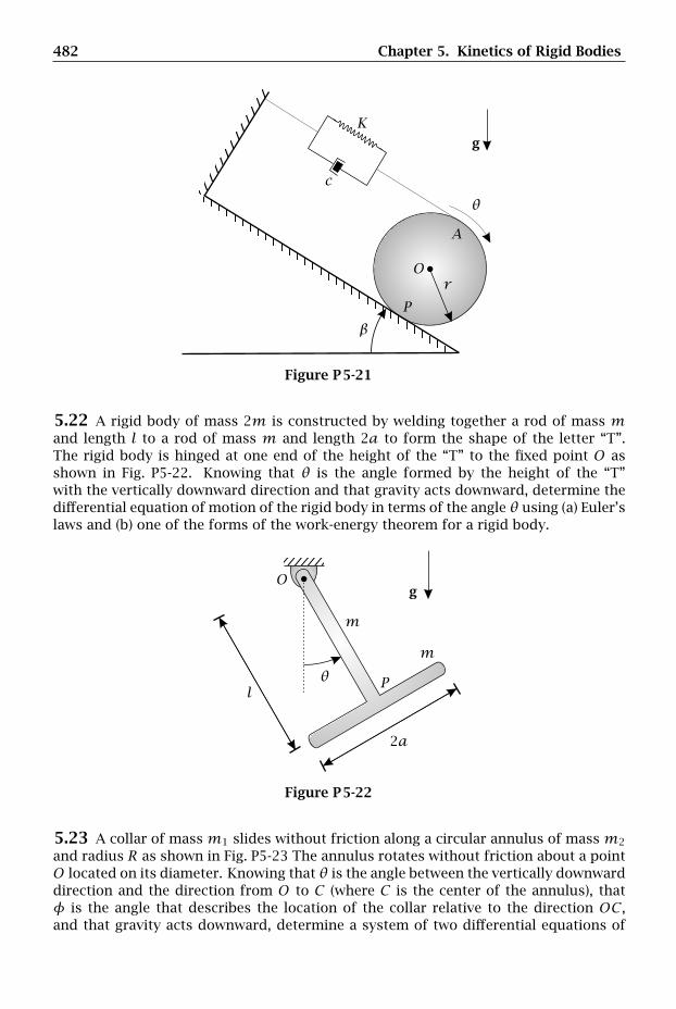
482 Chapter 5. Kinetics of Rigid Bodies
c
g
r
A
K
O
Pβ
θ
Figure P5-21
5.22 A rigid body of mass 2m is constructed by welding together a rod of mass mand length l to a rod of mass m and length 2a to form the shape of the letter “T”.The rigid body is hinged at one end of the height of the “T” to the fixed point O asshown in Fig. P5-22. Knowing that θ is the angle formed by the height of the “T”with the vertically downward direction and that gravity acts downward, determine thedifferential equation of motion of the rigid body in terms of the angle θ using (a) Euler’slaws and (b) one of the forms of the work-energy theorem for a rigid body.
g
l
2a
m
m
O
Pθ
Figure P5-22
5.23 A collar of massm1 slides without friction along a circular annulus of massm2
and radius R as shown in Fig. P5-23 The annulus rotates without friction about a pointO located on its diameter. Knowing that θ is the angle between the vertically downwarddirection and the direction from O to C (where C is the center of the annulus), thatφ is the angle that describes the location of the collar relative to the direction OC ,and that gravity acts downward, determine a system of two differential equations of

Problems for Chapter 5 483
motion for the collar and the annulus in terms of the variables θ and φ.
m1
m2
C
O
P
R
Rθ
φ
Figure P5-23
5.24 A slender uniform rod of mass m and length l is hinged at one of its endsat point Q to a massless collar. The collar simultaneously slides with known displace-ment y(t) along a vertical track and rotates with constant angular velocityΩ as shownin Fig. P5-24. Knowing that θ is the angle between the track and the rod and that grav-ity acts downward, determine the differential equation of motion for the rod in termsof the angle θ.
y(t)
g
l
m
Q
θ
Ω
Figure P5-24
5.25 A block of mass M , with a semicircular section of radius R cut out of its center,slides without friction along a horizontal surface. A homogeneous circular disk ofradius r rolls without slip along the circular surface cut out of the block as shown inFig. P5-25. Knowing that x describes the displacement of the block, that θ describesthe location of the center of the disk (point P ) relative to the center of the block (pointO), that φ describes the rotation of the disk relative to the direction OP , and thatgravity acts downward, determine a system of two differential equations of motion forthe block and disk in terms of the variables x and θ.

484 Chapter 5. Kinetics of Rigid Bodies
Frictionless
No Slipg
m
r
x
M
O
PQ
R
θ φ
Figure P5-25
5.26 A particle of massm slides without friction along a rod of mass M and length Las shown in Fig. P5-26. The particle is attached to a linear spring with spring constantK and unstretched length r0 while the rod is free to pivot about one of its ends atthe fixed hinge at point O. Knowing that the distance r describes the position of theparticle relative to pointO, that the angle θ describes the orientation of the rod relativeto the downward direction, and that gravity acts downward, determine a system of twodifferential equations of motion for the particle and the rod in terms of the variablesr and θ.
g
M,Lm
rK
O
θ
Figure P5-26
5.27 A system consists of an annulus of massm and radius R and a uniform circulardisk of mass m and radius r as shown in Fig. P5-27. The annulus rolls without slipalong a fixed horizontal surface while the disk rolls without slip along the inner surfaceof the annulus. Knowing that the angle θ describes the rotation of the annulus relativeto the ground, that the angle φ describes the location of the center of mass of thedisk relative to the center of the annulus, and that gravity acts downward, determinea system of two differential equations for the annulus and the disk in terms of theangles θ and φ.
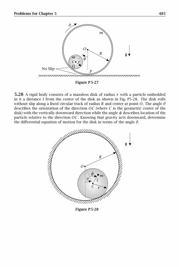
Problems for Chapter 5 485
No Slip
gm
m
rC
O
PQ
R
θ
φ
Figure P5-27
5.28 A rigid body consists of a massless disk of radius r with a particle embeddedin it a distance l from the center of the disk as shown in Fig. P5-28. The disk rollswithout slip along a fixed circular track of radius R and center at point O. The angle θdescribes the orientation of the direction OC (where C is the geometric center of thedisk) with the vertically downward direction while the angleφ describes location of theparticle relative to the direction OC . Knowing that gravity acts downward, determinethe differential equation of motion for the disk in terms of the angle θ.
g
lm
rC
O
R
θφ
Figure P5-28

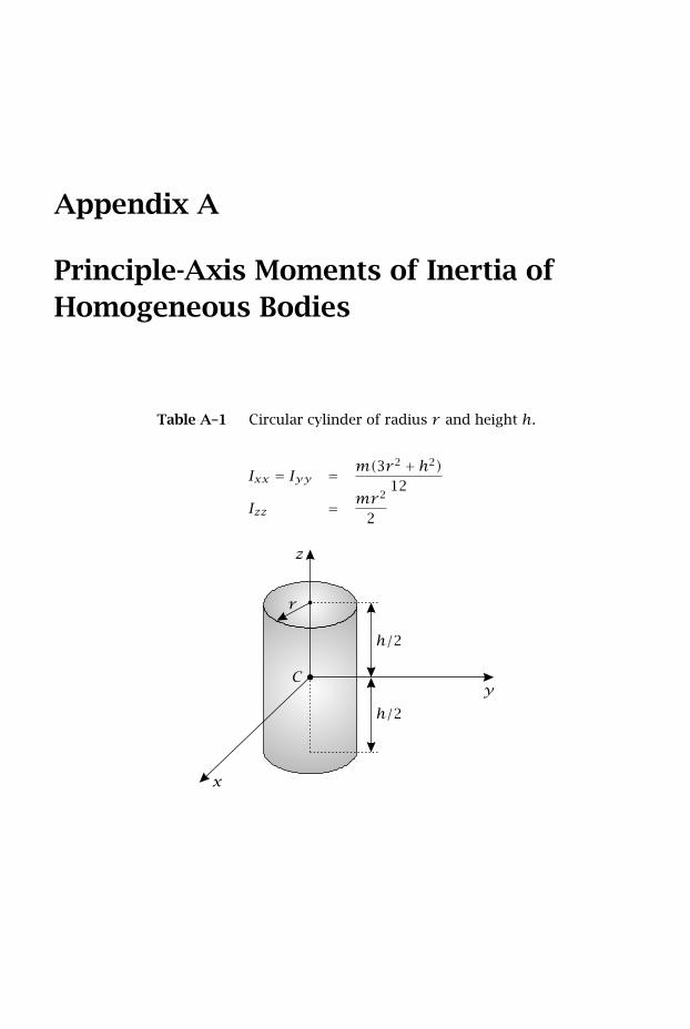
Appendix A
Principle-Axis Moments of Inertia ofHomogeneous Bodies
Table A–1 Circular cylinder of radius r and height h.
Ixx = Iyy = m(3r 2 + h2)12
Izz = mr 2
2
h/2
h/2
r
x
y
z
C
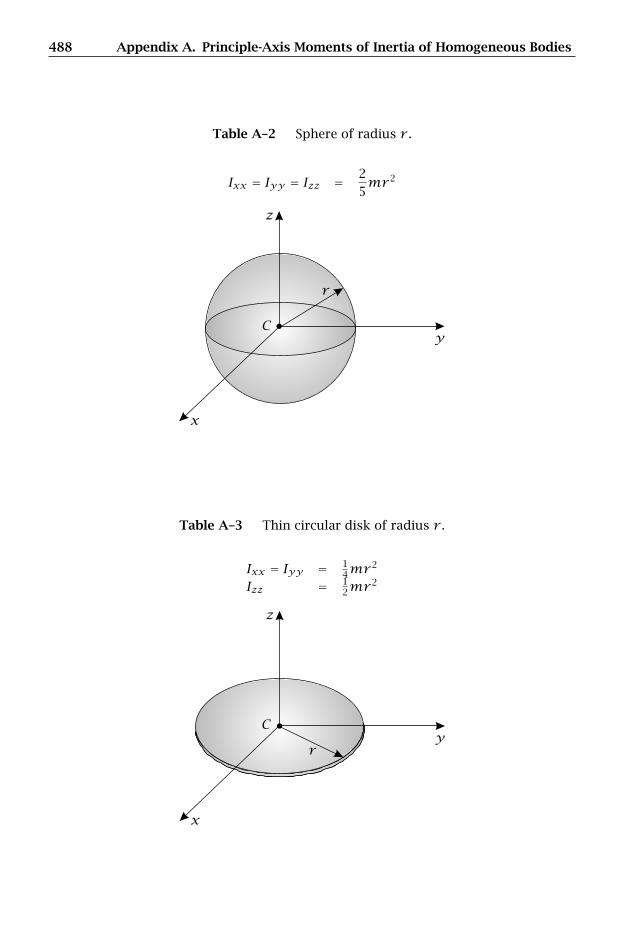
488 Appendix A. Principle-Axis Moments of Inertia of Homogeneous Bodies
Table A–2 Sphere of radius r .
Ixx = Iyy = Izz = 25mr 2
r
x
y
z
C
Table A–3 Thin circular disk of radius r .
Ixx = Iyy = 14mr
2
Izz = 12mr
2
r
x
y
z
C
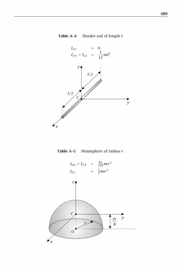
489
Table A–4 Slender rod of length l.
Ixx = 0
Iyy = Izz = 112ml2
l/2
l/2
x
y
z
C
Table A–5 Hemisphere of radius r .
Ixx = Iyy = 83320mr
2
Izz = 25mr
2
r
x
y
z
C
O
3r8
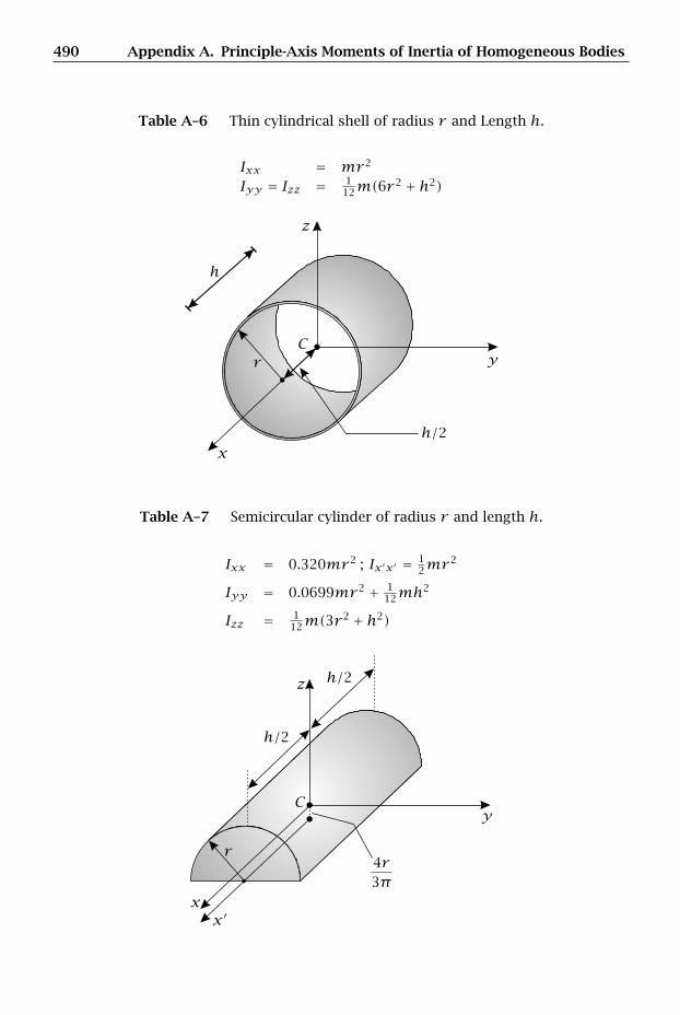
490 Appendix A. Principle-Axis Moments of Inertia of Homogeneous Bodies
Table A–6 Thin cylindrical shell of radius r and Length h.
Ixx = mr 2
Iyy = Izz = 112m(6r
2 + h2)
h/2
r
h
x
y
z
C
Table A–7 Semicircular cylinder of radius r and length h.
Ixx = 0.320mr 2 ; Ix′x′ = 12mr
2
Iyy = 0.0699mr 2 + 112mh
2
Izz = 112m(3r
2 + h2)
h/2
h/2
r
xx′
y
z
C
4r3π
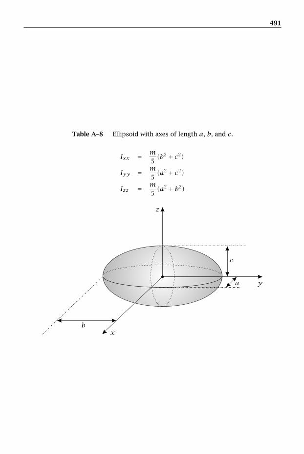
491
Table A–8 Ellipsoid with axes of length a, b, and c.
Ixx = m5(b2 + c2)
Iyy = m5(a2 + c2)
Izz = m5(a2 + b2)
c
a
bx
y
z

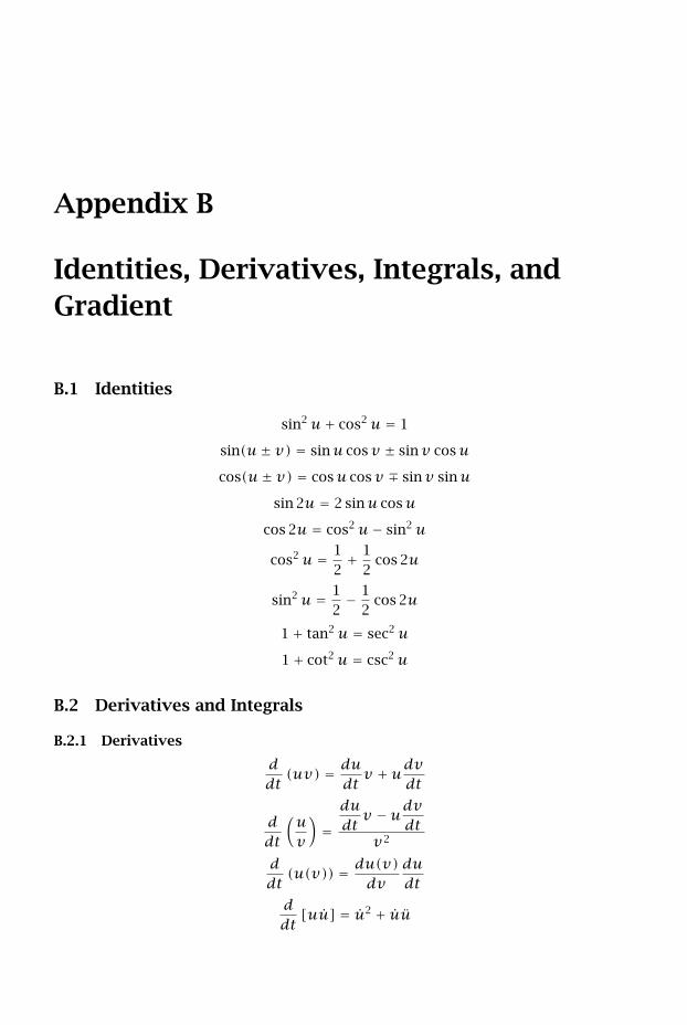
Appendix B
Identities, Derivatives, Integrals, andGradient
B.1 Identities
sin2u+ cos2u = 1
sin(u± v) = sinu cosv ± sinv cosu
cos(u± v) = cosu cosv ∓ sinv sinu
sin 2u = 2 sinu cosu
cos 2u = cos2u− sin2u
cos2u = 12+ 1
2cos 2u
sin2u = 12− 1
2cos 2u
1+ tan2u = sec2u
1+ cot2u = csc2u
B.2 Derivatives and Integrals
B.2.1 Derivatives
ddt(uv) = du
dtv +udv
dt
ddt
(uv
)=dudtv −udv
dtv2
ddt(u(v)) = du(v)
dvdudt
ddt[uu] = u2 + uu
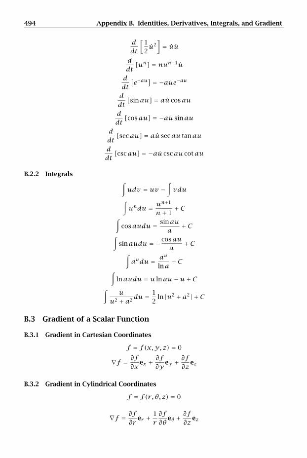
494 Appendix B. Identities, Derivatives, Integrals, and Gradient
ddt
[12u2]= uu
ddt[un] = nun−1u
ddt
[e−au
] = −aue−auddt[sinau] = au cosau
ddt[cosau] = −au sinau
ddt[secau] = au secau tanau
ddt[cscau] = −au cscau cotau
B.2.2 Integrals ∫udv = uv −
∫vdu
∫undu = u
n+1
n+ 1+ C
∫cosaudu = sinau
a+ C
∫sinaudu = −cosau
a+ C
∫audu = au
lna+ C
∫lnaudu = u lnau−u+ C
∫u
u2 + a2du = 1
2ln |u2 + a2| + C
B.3 Gradient of a Scalar Function
B.3.1 Gradient in Cartesian Coordinates
f = f(x,y, z) = 0
∇f = ∂f∂x
ex + ∂f∂y ey + ∂f∂z ez
B.3.2 Gradient in Cylindrical Coordinates
f = f(r , θ, z) = 0
∇f = ∂f∂r
er + 1r∂f∂θ
eθ + ∂f∂z ez
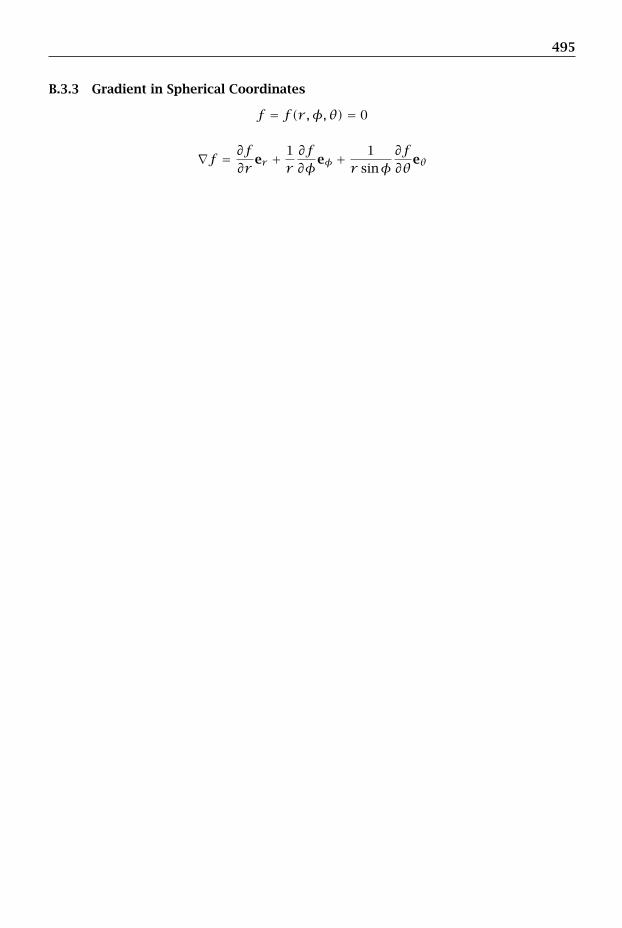
495
B.3.3 Gradient in Spherical Coordinates
f = f(r ,φ,θ) = 0
∇f = ∂f∂r
er + 1r∂f∂φ
eφ + 1r sinφ
∂f∂θ
eθ


Appendix C
Answers to Selected Problems
Chapter 2
2.1 Fv = v0ex +ΩreyFa = −Ω2rex + 2Ωv0ey
2.2 Fv = rer + r(Ω + θ)eθFa =
[r − r(Ω + θ)2
]er +
[r θ + 2r (Ω + θ)
]eθ
2.3 Fv = rer + r θeθ + rΩ sinθez
Fa = (r − r θ2 − rΩ2 sin2θ)er + (2r θ + r θ − rΩ2 cosθ sinθ)eθ
+2Ω(r sinθ + r θ cosθ)ez
2.4 Fv = xex + (2xx/a)ey −ΩxezFa = (x −Ω2x)ex +
[2(x2 + xx)/a]ey − 2Ωxez
2.5 Fv = (x −Ωy)ex + (y +Ωx)ey + zezFa = (x − 2Ωy −Ω2x)ex + (y + 2Ωx −Ω2y)ey + zez
2.8 (a) Fs = Fs0 + R secφ(θ − θ0)
(b) et = cosφeθ + sinφez; en = −er ; eb = − sinφeθ + cosφez
(c) Fv = Rθ secφet ; Fa = Rθ secφet + Rθ2en
2.9 FvP = l2 θ cosθex − l2 θ sinθey − l2Ω sinθez
FaP = − lΩ2
2sinθex −
v20
2l cos3 θey −
[v0Ω + lΩ sinθ
2
]ez
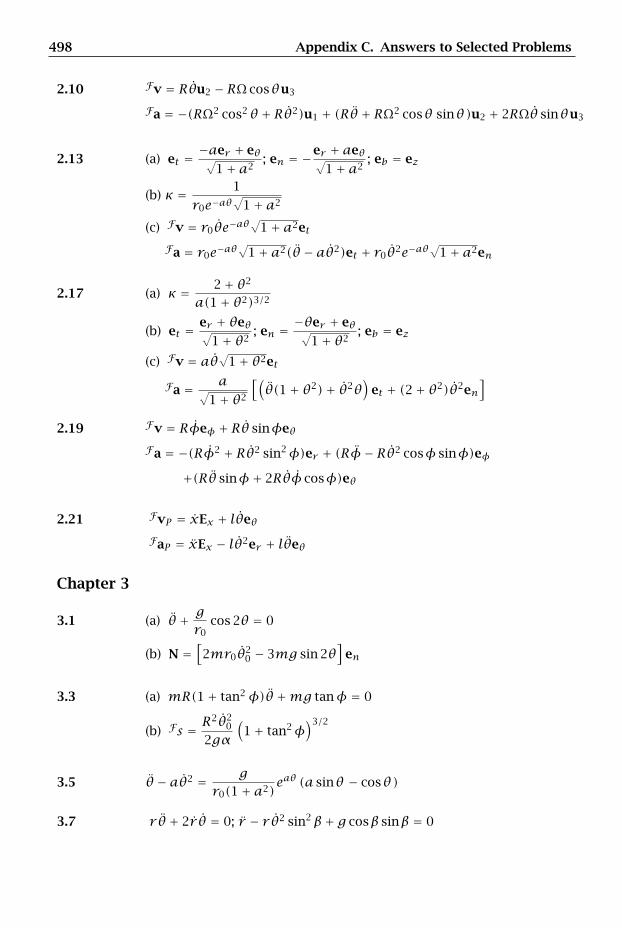
498 Appendix C. Answers to Selected Problems
2.10 Fv = Rθu2 − RΩ cosθu3
Fa = −(RΩ2 cos2θ + Rθ2)u1 + (Rθ + RΩ2 cosθ sinθ)u2 + 2RΩθ sinθu3
2.13 (a) et = −aer + eθ√1+ a2
; en = −er + aeθ√1+ a2
; eb = ez
(b) κ = 1
r0e−aθ√
1+ a2
(c) Fv = r0θe−aθ√
1+ a2et
Fa = r0e−aθ√
1+ a2(θ − aθ2)et + r0θ2e−aθ√
1+ a2en
2.17 (a) κ = 2+ θ2
a(1+ θ2)3/2
(b) et = er + θeθ√1+ θ2
; en = −θer + eθ√1+ θ2
; eb = ez
(c) Fv = aθ√
1+ θ2et
Fa = a√1+ θ2
[(θ(1+ θ2)+ θ2θ
)et + (2+ θ2)θ2en
]
2.19 Fv = Rφeφ + Rθ sinφeθ
Fa = −(Rφ2 + Rθ2 sin2φ)er + (Rφ− Rθ2 cosφ sinφ)eφ
+(Rθ sinφ+ 2Rθφ cosφ)eθ
2.21 FvP = xEx + lθeθ
FaP = xEx − lθ2er + lθeθ
Chapter 3
3.1 (a) θ + gr0
cos 2θ = 0
(b) N =[2mr0θ2
0 − 3mg sin 2θ]
en
3.3 (a) mR(1+ tan2φ)θ +mg tanφ = 0
(b) Fs = R2θ2
0
2gα
(1+ tan2φ
)3/2
3.5 θ − aθ2 = gr0(1+ a2)
eaθ (a sinθ − cosθ)
3.7 r θ + 2r θ = 0; r − r θ2 sin2β+ g cosβ sinβ = 0

499
3.9 (a) θ2 + θθ −Ω2 = 0
(b) T = [4mRΩ3t
]ey
3.10 m secx[x + x2 tanx
] = −mg sinx
3.11 r − r θ2 + Km(r − L) = 0; r θ + 2r θ = 0
3.12 m[r − r θ2 − lω2 cos(θ −ωt)]+K(r − r0) = 0
m[2r θ + r θ + lω2 sin(θ −ωt)] = 0
3.13 r θ + 2r θ = 0;
[1+
(rR
)2]r + r
R2r 2 − r θ2 + gr
R= 0
3.17 (l− Rθ)θ − Rθ2 − g cosθ = 0
3.19 (a) θ − 2Km
sinθ = 0
(b) N =[−mRθ2
0 − 4KR cosθ 0 + 6KR cosθ +KR]
er
3.20 m(r − r θ2) = −F ; 2r θ + r θ = 0
3.23 r − rΩ2 sin2β+ cr + g cosβ = 0
Chapter 4
4.2 (a) Fm =mv0 cosθM
m+M Ex +mv0 sinθEy
(b) Fv′m = Fv′M =m
m+Mv0 cosθEx
4.3 (a) Fvm = Fvm = mm+M
√2ghEx
(b) xmax = (m+M)g3K
[1+
√1+ 6Kh
(m+M)g
]
4.6 (a) Fv′A =mA − emB
mA +mBv0Ex ; Fv′B =
mA(1+ e)mA +mB
v0Ex
(b) v0 = 2(mA +mB)mA(1+ e)
√gr
4.8 (mA cos2θ +mB sin2θ)lθ + (mA −mB)lθ2 cosθ sinθ −mAg cosθ = 0
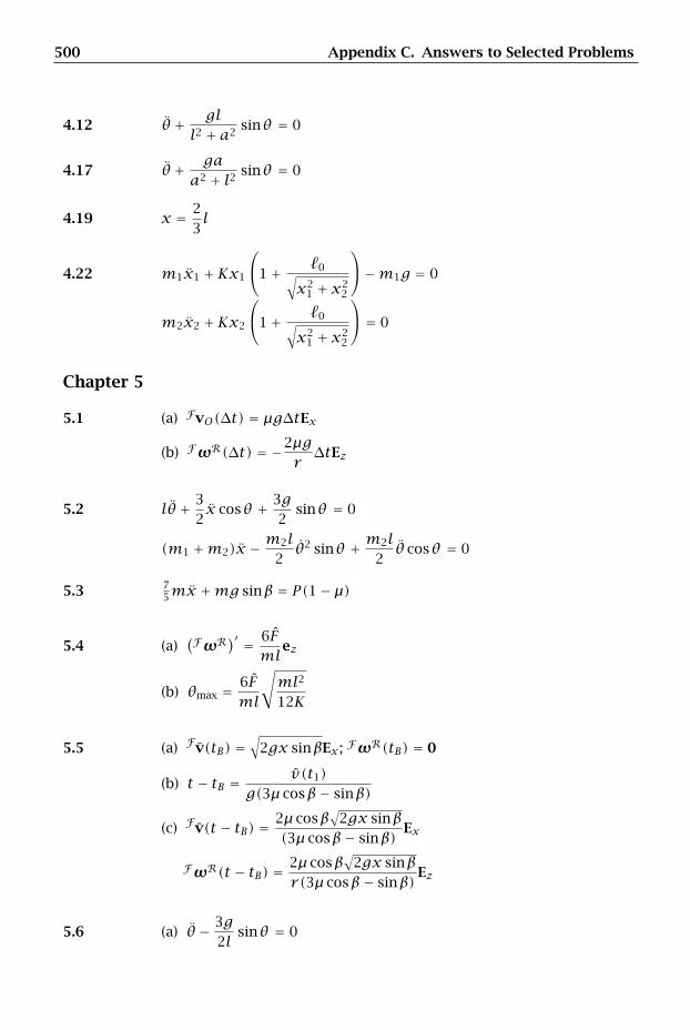
500 Appendix C. Answers to Selected Problems
4.12 θ + gll2 + a2
sinθ = 0
4.17 θ + gaa2 + l2 sinθ = 0
4.19 x = 23l
4.22 m1x1 +Kx1
⎛⎝1+ 0√
x21 + x2
2
⎞⎠−m1g = 0
m2x2 +Kx2
⎛⎝1+ 0√
x21 + x2
2
⎞⎠ = 0
Chapter 5
5.1 (a) FvO(∆t) = µg∆tEx
(b) FωR(∆t) = −2µgr∆tEz
5.2 lθ + 32x cosθ + 3g
2sinθ = 0
(m1 +m2)x − m2l2θ2 sinθ + m2l
2θ cosθ = 0
5.3 75mx +mg sinβ = P(1− µ)
5.4 (a)(FωR)′ = 6F
mlez
(b) θmax = 6Fml
√ml2
12K
5.5 (a) Fv(tB) =√
2gx sinβEx ; FωR(tB) = 0
(b) t − tB = v(t1)g(3µ cosβ− sinβ)
(c) Fv(t − tB) = 2µ cosβ√
2gx sinβ(3µ cosβ− sinβ)
Ex
FωR(t − tB) = 2µ cosβ√
2gx sinβr(3µ cosβ− sinβ)
Ez
5.6 (a) θ − 3g2l
sinθ = 0
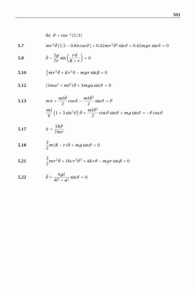
501
(b) θ = cos−1(2/3)
5.7 mr 2θ [1.5− 0.84 cosθ]+ 0.42mr 2θ2 sinθ + 0.42mgr sinθ = 0
5.8 θ − 5g7r
sin(rθR + r
)= 0
5.10 32mr
2θ +Kr 2θ −mgr sinβ = 0
5.12 (3ma2 +ml2)θ + 3mga sinθ = 0
5.13 mx + mlθ2
cosθ − mlθ2
2sinθ = P
ml6
(1+ 3 sin2θ
)θ + mlθ
2
2cosθ sinθ +mg sinθ = −P cosθ
5.17 x = 5hP7mr
5.1832m(R − r)θ +mg sinθ = 0
5.2132mr 2θ + 16cr 4θ3 + 4Krθ −mgr sinβ = 0
5.22 θ + 6gl4l2 + a2
sinθ = 0

Bibliography
Baruh, H. (1999), Analytical Dynamics, McGraw-Hill, New York.
Bedford, A. and Fowler, W. (2005), Engineering Dynamics: Mechanics Principles,Prentice-Hall, Upper Saddle River, NJ.
Beer, F. P. and Johnston, E. R. (1997), Vector Mechanics for Engineers: Dynamics, SixthEdition, McGraw-Hill, New York.
Coulomb, C. A. (1785), “Theorie Des Machines Simples En Ayant Egard Au Frottementet a La Roideur Des Cordages,” Memoires de Mathematique et de Physique Presentes aL’Academie Royale des Sciences Par Divers Savans, et Lus Dan Ses Assembles, Vol. 10,pp. 161–332.
Frenet, J-F. (1852), “Sur Quelques Proprietes Des Courbes a La Double Courbure,” Jour-nal De Mathematiques Pures et Appliquees, Vol. 17, pp. 437–447.
Greenwood, D. T. (1977), Classical Dynamics, Prentice-Hall, Upper Saddle River, NJ.
Greenwood, D. T. (1988), Principles of Dynamics, Prentice-Hall, Upper Saddle River, NJ.
Hibbeler, R. C. (2001), Engineering Mechanics: Dynamics, Ninth Edition, Prentice-Hall,Upper Saddle River, NJ.
Huygens, C. (1673), “Horologium Oscillatorium, Sive de Motu Pendulorum ad HorologiaAptato,” Paris. English translation in by Blackwell, R. J. (1986) “The Pendulum Clock,or, Geometrical Demonstrations Concerning the Motion of Pendula as Applied toClocks, Series in the History of Technology and Science,” Iowa State University Press,Ames, IA.
Kane,T. R. and Levinson, D. A. (1985), Dynamics: Theory and Applications, McGraw-Hill,New York.
Kreyszig, E. (1988), Advanced Engineering Mathematics, John Wiley & Sons, New York.
Merriam, J. L. and Kraige, L. G. (1997), Engineering Mechanics: Dynamics, Fourth Edi-tion, John Wiley & Sons, New York.
Newton, I. (1687), Philosophiae Naturalis Principia Mathematica, English Translation byMotte, A. (1729), Revised Translation by Cajori, F. (1934), published by The Univer-sity of California Press, Berkeley, California.
O’Reilly, O. M. (2001), Engineering Dynamics: A Primer, Springer-Verlag, New York.

504 Bibliography
O’Reilly, O. M. and Srinivasa, A. R. (2002), On Potential Energies and Constraints of RigidBodies and Particles, Mathematical Problems in Engineering, Vol. 8, No. 1, pp. 169–180.
O’Reilly, O. M. (2004), Lecture Notes on the Dynamics of Particles and Rigid Bodies: ClassNotes for Engineering Mechanics III and Intermediate Dynamics ME 175, Departmentof Mechanical Engineering, University of California, Berkeley.
Papastavridis, J. G. (2002), Analytical Mechanics: A Comprehensive Treatise on the Dy-namics of Constrained Systems: For Engineers, Physicists, and Mathematicians, Ox-ford University Press, New York.
Serret, J. A. (1851), “Sur Quelque Formule Reletives a La Theorie Des Courbes a DoubleCourbure,” Journal De Mathematiques Pures et Appliquees, Vol. 16, pp. 193–207.
Synge, J. L. and Griffith, B. L. (1959), Principles of Mechanics, McGraw-Hill, New York.
Tenenbaum, R. A. (2004), Fundamentals of Applied Dynamics, Springer-Verlag, NewYork.
Thomas, G. B. and Finney, R. L. (2002), Calculus and Analytic Geometry, Addison-Wesley Publishing Company, New York.
Thornton, S. T. and Marion, J. B. (2004), Classical Dynamics of Particles and Systems,Brooks/Cole Publishing, Belmont, California.
Index
R, 3R3, 3
Acceleration, 36, 50as a function of position, 41as a function of time, 40as a function of velocity, 41centripetal, 88Coriolis, 88Euler, 88in a rotating reference frame, 50in Cartesian coordinates, 52in cylindrical coordinates, 56in intrinsic coordinates, 74in spherical coordinates, 67of Center of Mass
for a system of particles, 240relative, 39
Addition of angular velocities, 48Angular acceleration, 48, 49Angular impulse, 180, 181, 267, 441
for a particle, 180, 181for a system of particles, 267of a rigid body, 441
Angular momentum, 179conservation of, 181
in all directions, 181of a particle, 179of a rigid body, 323
relative to a point fixed in an in-ertial reference frame, 324
relative to an arbitrary referencepoint, 323
relative to the center of mass, 324of a system of particles, 240
relative to an inertially fixed point,240
relative to the center of mass, 240rate of change
for a particle, 179, 180
for a rigid body, 355, 356for a system of particles, 249
Angular velocity, 46addition, 48definition of, 46in cylindrical coordinates, 55in intrinsic coordinates, 72, 74in spherical coordinates, 67
Arc-length, 36, 75
Body-fixed reference frame, see Refer-ence frame
Cartesian coordinates, see Coordinate sys-tems
Center of Massof a system of particles, 238
Central force, 153Coefficient of restitution, 291, 452Collision, 289
of particles, 289model, 289notes on, 298
of rigid bodies, 450model, 450
Column-vector, see VectorConservation of angular momentum, 181Conservation of energy, 195, 197
for a particle, 195, 197for a rigid body, 426
Conservation of linear momentum, 177Conservative force, 190
Examples, 192Constant force
Potential Energy of, 192Contact force, 146Coordinate axes
translation, 330Coordinate system, 30
fixed in a rigid body, 104Coordinate systems, 51, 72

506 Index
Cartesian, 51acceleration, 52position, 51velocity, 52
cylindricalacceleration, 56angular velocity, 55position, 55velocity, 56
intrinsic, 71, 72acceleration, 71angular velocity, 72formulas, 76position, 71velocity, 71
sphericalacceleration, 67angular velocity, 67position, 67velocity, 67
Couple, 350, 351Cross product, see Vector productCylindrical coordinates, see Coordinate
systems
Determinant, 23Differential equation, see Ordinary dif-
ferential equationDirac delta function, 187Dot product, see Scalar productDual Euler basis, 120
Eigenvalue, 22Eigenvector, 22Energy, 188
kinetic, 189Euler angles, 113
classes of, 120gimbal lock, 120
Euler basis, 120Euler’s first law, 355Euler’s laws, 355Euler’s second law, 355
relative to a fixed point, 355, 357relative to an arbitrary reference point,
355, 357relative to the center of mass, 356,
357Eulerian angles, 113
Forcecentral, 153conservative, 190gravitational, 153of friction, 146of gravity, 154power of, see Power of a forcespring, 150
Friction force, 146, 149Coulomb, 149viscous, 149
Galilean invariance, 30Gimbal lock, see Euler anglesGravitational force
Potential energy of, 194
Hooke’s law, 150Huygens-Steiner theorem, see Parallel-
axis theorem
Identity Matrix, see MatrixIdentity tensor, see TensorImpact, 289, 450
inelastic, 294of particles
model, 289of rigid bodies, 450perfectly elastic, 294perfectly inelastic, 294phases of, 289, 450
compression, 289, 450restitution, 289, 450
Impulseangular, 180instantaneous, 187linear, 176
Instantaneous center of rotation, 364Invariance
of space, 29of time, 30
Inverse of a matrix, see MatrixInverse of a tensor, see Tensor
Kinematics, 27of particles, 27
Kinetic energy, 189, 419for a rigid body, 419for a system of particles, 280
Kinetics
507
of a system of particles, 237of particles, 145of rigid bodies, 321
Koenig’s decomposition, 281, 421for a rigid body, 421for a system of particles, 281
Linear equationssystem of, 14
Linear impulse, 176, 266, 441for a particle, 176for a rigid body, 441for a system of particles, 266
Linear momentum, 176, 441conservation of, 177
in all directions, 177in an inertially fixed direction, 178
for a particle, 176for a rigid body, 441of a rigid body, 441of a system of particles, 239
Matrix, 14, 15definition of, 14identity, 15inverse, 15orthogonal, 15skew-symmetric, 15symmetric, 15, 23transpose, 15
Moment, 178definition, 178inertial, 250, 356, 357of a force, 178
Moment of a forcefor a system of particles, 248
relative to an arbitrary point, 248relative to the center of mass of
the system, 248Moment of inertia, 325
cylinder, 487ellipsoid, 487hemisphere, 487semi-circular cylinder, 487slender rod, 487sphere, 487thin circular disk, 487thin cylindrical shell, 487
Moment of inertia tensor, 325, 326
Moment transport theorem, 178, 353,354
for a particle, 178for a rigid body, 353, 354
Newton’s first law, 157Newton’s laws, 157
for a particle, 157for a system of particles, 242
Newton’s second law, 157Newton’s third law, 157Newtonian relativity, 30
Observers, 28Ordinary differential equation, 25Orthogonal matrix, see MatrixOrthogonal tensor, see Tensor
Parallel-axis theorem, 330, 333Particle, 35
acceleration, 36definition of, 35position, 35trajectory, 35velocity, 36
Point fixed in a reference frame, 36Position, 35
in Cartesian coordinates, 51in cylindrical coordinates, 55in intrinsic coordinates, 71in spherical coordinates, 67relative, 39
Power of a force, 188Principal-axis basis, 335Principal-axis coordinate system, 334Principal-axis moments of inertia, 337Principle of angular impulse and angu-
lar momentum, 180, 181, 267,441
for a particle, 180, 181for a rigid body, 441for a system of particles, 267
Principle of linear impulse and linearmomentum, 176, 266, 441
for a particle, 176for a rigid body, 441for a system of particles, 266
Principle of work and energy, 190, 197,424, 426
alternate form
508 Index
for a particle, 197for a rigid body, 426
for a particle, 190, 197for a rigid body, 424
Pure torque, 350, 351applied to a rigid body, 350, 351conservative, 352definition of, 350, 351power of, 352translation between points on a rigid
body, 351work of, 352
Rate of changeof a scalar function, 32of a vector function, 32, 33
Rate of change transport theorem, 47Rectilinear motion, 39Reference frame, 28
fixed in a rigid body, 104Reference frames, 28
fixed, 30inertial, 30moving, 30Newtonian, 30non-Newtonian, 30noninertial, 30rotating and translating, 85
Right-hand rule, 8, 31Right-handed sense, 8Right-handed system, 31Rigid body
angular velocity, 104as a reference frame, 104definition of, 104extension, 104orientation, 113velocity and acceleration of points
on, 105Rigidly connected points, 28Row-vector, see Vector
Scalar, 2definition of, 2notation, 2
Scalar Product, 7Scalar product, 7
properties of, 7Scalar triple product, 9
Serret-Frenet coordinates, see Coordinatesystems
Serret-Frenet formulas, 76Skew-symmetric matrix, see MatrixSkew-symmetric tensor, see TensorSpherical coordinates, see Coordinate sys-
temsSpring force, 150
definition of, 150potential energy of, 193
Symmetric matrix, see Matrix, see Ma-trix
Symmetric tensor, see TensorSystems of particles, 237
Tensor, 10basis representation of, 12definition of, 10identity tensor, 10inverse, 11matrix representation of, 16orthogonal, 11properties of, 10relationship to matrices, 15skew-symmetric, 11symmetric, 11transpose, 11zero tensor, 10
Tensor product, 11Transport theorem, 47
for the rate of change of a vector,47
Transpose of a matrix, see MatrixTranspose of a tensor, see Tensor
Universal law of gravitation, 153
Vector, 3addition, 4
properties of, 4bound, 3, 4column, 14components of, 6definition of, 3direction, 3fixed in a reference frame, 33free, 3, 4length, 3magnitude, 3
509
multiplication by a scalar, 6properties of, 7
mutual orthogonality, 7, 31notation, 3orthogonality, 7, 31rate of change of, 42, 47
in a rotating reference frame, 42,47
row, 15scalar product, 7scalar triple product, 9sliding, 3, 4time derivative of
in a rotating and translating ref-erence frame, 85
unit vector, 3vector triple product, 10
Vector product, 8in determinant form, 9properties of, 8
Vector triple product, 10Velocity, 36, 50
in a rotating and translating refer-ence frame, 85, 86
in a rotating reference frame, 50in Cartesian coordinates, 52in cylindrical coordinates, 56in intrinsic coordinates, 71in spherical coordinates, 67of Center of Mass
for a system of particles, 239relative, 39
Work, 188Work and energy, 280, 419
for a rigid body, 419for a system of particles, 280
Work-energy theorem, 189, 422alternate form
for a particle, 195for a rigid body, 424, 425for a system of particles, 283, 284
for a particle, 189for a rigid body, 422for a system of particles, 281, 282
Zero tensor, see TensorZero vector, 3