Introduction 5.1Synchronous machines 5.2

Armature reaction 5.3Steady state theory 5.4

Salient pole rotor 5.5Transient analysis 5.6

Asymmetry 5.7Machine reactances 5.8

Negative sequence reactance 5.9Zero sequence reactance 5.10

Direct and quadrature axis values 5.11Effect of saturation on machine reactances 5.12

Transformers 5.13Transformer positive sequence equivalent circuits 5.14

Transformer zero sequence equivalent circuits 5.15Auto-transformers 5.16

Transformer impedances 5.17Overhead lines and cables 5.18

Calculation of series impedance 5.19Calculation of shunt impedance 5.20

Overhead line circuits with or without earth wires 5.21OHL equivalent circuits 5.22

Cable circuits 5.23Overhead line and cable data 5.24

References 5.25

• 5 • E q u i v a l e n t C i r c u i t s a n d P a r a m e t e r s o f P o w e r S y s t e m P l a n t

N e t w o r k P r o t e c t i o n & A u t o m a t i o n G u i d e • 4 7 •

5.1 INTRODUCTION

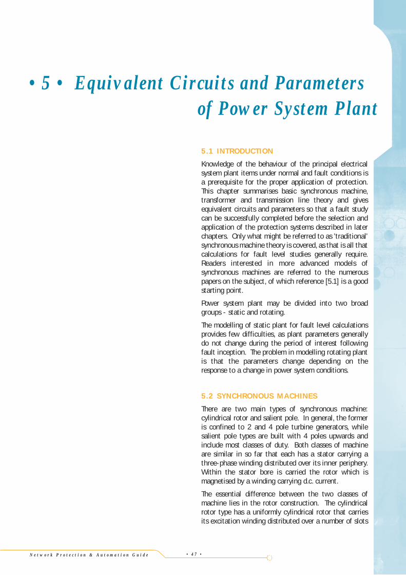
Knowledge of the behaviour of the principal electricalsystem plant items under normal and fault conditions isa prerequisite for the proper application of protection.This chapter summarises basic synchronous machine,transformer and transmission line theory and givesequivalent circuits and parameters so that a fault studycan be successfully completed before the selection andapplication of the protection systems described in laterchapters. Only what might be referred to as 'traditional'synchronous machine theory is covered, as that is all thatcalculations for fault level studies generally require.Readers interested in more advanced models ofsynchronous machines are referred to the numerouspapers on the subject, of which reference [5.1] is a goodstarting point.

Power system plant may be divided into two broadgroups - static and rotating.

The modelling of static plant for fault level calculationsprovides few difficulties, as plant parameters generallydo not change during the period of interest followingfault inception. The problem in modelling rotating plantis that the parameters change depending on theresponse to a change in power system conditions.

5.2 SYNCHRONOUS MACHINES

There are two main types of synchronous machine:cylindrical rotor and salient pole. In general, the formeris confined to 2 and 4 pole turbine generators, whilesalient pole types are built with 4 poles upwards andinclude most classes of duty. Both classes of machineare similar in so far that each has a stator carrying athree-phase winding distributed over its inner periphery.Within the stator bore is carried the rotor which ismagnetised by a winding carrying d.c. current.

The essential difference between the two classes ofmachine lies in the rotor construction. The cylindricalrotor type has a uniformly cylindrical rotor that carriesits excitation winding distributed over a number of slots

• 5 • Equ iva lent Cir cuits an d Parame te rs o f Pow e r Sys te m P lant

most common. Two-stroke diesel engines are oftenderivatives of marine designs with relatively large outputs(circa 30MW is possible) and may have running speeds ofthe order of 125rpm. This requires a generator with alarge number of poles (48 for a 125rpm, 50Hz generator)and consequently is of large diameter and short axiallength. This is a contrast to turbine-driven machines thatare of small diameter and long axial length.

N e t w o r k P r o t e c t i o n & A u t o m a t i o n G u i d e

• 5 •

Equi

valen

tCirc

uits

andP

aram

eters

ofPo

wer

Syste

mPl

ant

around its periphery. This construction is unsuited tomulti-polar machines but it is very sound mechanically.Hence it is particularly well adapted for the highestspeed electrical machines and is universally employed for2 pole units, plus some 4 pole units.

The salient pole type has poles that are physicallyseparate, each carrying a concentrated excitationwinding. This type of construction is in many wayscomplementary to that of the cylindrical rotor and isemployed in machines having 4 poles or more. Except inspecial cases its use is exclusive in machines having morethan 6 poles. Figure 5.1 illustrates a typical largecylindrical rotor generator installed in a power plant.

Two and four pole generators are most often used inapplications where steam or gas turbines are used as thedriver. This is because the steam turbine tends to besuited to high rotational speeds. Four pole steam turbinegenerators are most often found in nuclear powerstations as the relative wetness of the steam makes thehigh rotational speed of a two-pole design unsuitable.Most generators with gas turbine drivers are four polemachines to obtain enhanced mechanical strength in therotor- since a gearbox is often used to couple the powerturbine to the generator, the choice of synchronousspeed of the generator is not subject to the sameconstraints as with steam turbines.

Generators with diesel engine drivers are invariably offour or more pole design, to match the running speed ofthe driver without using a gearbox. Four-stroke dieselengines usually have a higher running speed than two-stroke engines, so generators having four or six poles are

Strong

N S

Direction of rotation

(a)

(b)

S NN

Weak Weak Strong

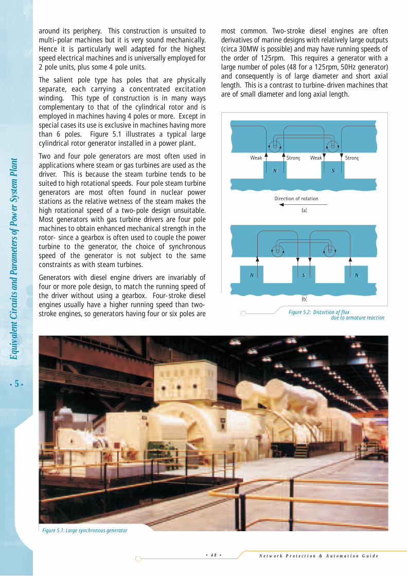
Figure 5.2: Distortion of fluxdue to armature reaction

• 4 8 •

Figure 5.1: Large synchronous generator

N e t w o r k P r o t e c t i o n & A u t o m a t i o n G u i d e • 4 9 •

• 5 •

5.3 ARMATURE REACTION

Armature reaction has the greatest effect on theoperation of a synchronous machine with respect both tothe load angle at which it operates and to the amount ofexcitation that it needs. The phenomenon is most easilyexplained by considering a simplified ideal generatorwith full pitch winding operating at unity p.f., zero lagp.f. and zero lead p.f. When operating at unity p.f., thevoltage and current in the stator are in phase, the statorcurrent producing a cross magnetising magneto-motiveforce (m.m.f.) which interacts with that of the rotor,resulting in a distortion of flux across the pole face. Ascan be seen from Figure 5.2(a) the tendency is to weakenthe flux at the leading edge or effectively to distort thefield in a manner equivalent to a shift against thedirection of rotation.

If the power factor were reduced to zero lagging, thecurrent in the stator would reach its maximum 90° afterthe voltage and the rotor would therefore be in theposition shown in Figure 5.2(b). The stator m.m.f. is nowacting in direct opposition to the field.

Similarly, for operation at zero leading power factor, thestator m.m.f. would directly assist the rotor m.m.f. Thism.m.f. arising from current flowing in the stator is knownas 'armature reaction'.

5.4 . STEADY STATE THEORY

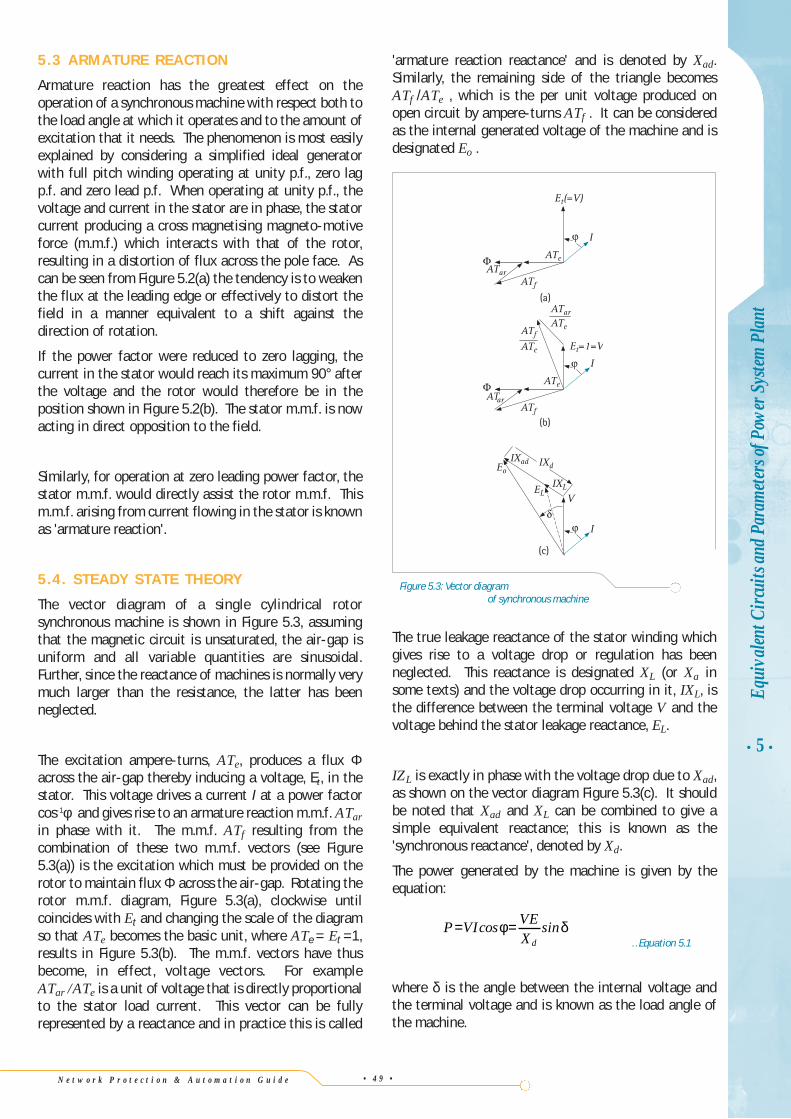
The vector diagram of a single cylindrical rotorsynchronous machine is shown in Figure 5.3, assumingthat the magnetic circuit is unsaturated, the air-gap isuniform and all variable quantities are sinusoidal.Further, since the reactance of machines is normally verymuch larger than the resistance, the latter has beenneglected.

The excitation ampere-turns, ATe, produces a flux Φacross the air-gap thereby inducing a voltage, Et, in thestator. This voltage drives a current I at a power factorcos-1φ and gives rise to an armature reaction m.m.f. ATarin phase with it. The m.m.f. ATf resulting from thecombination of these two m.m.f. vectors (see Figure5.3(a)) is the excitation which must be provided on therotor to maintain flux Φ across the air-gap. Rotating therotor m.m.f. diagram, Figure 5.3(a), clockwise untilcoincides with Et and changing the scale of the diagramso that ATe becomes the basic unit, where ATe = Et =1,results in Figure 5.3(b). The m.m.f. vectors have thusbecome, in effect, voltage vectors. For exampleATar /ATe is a unit of voltage that is directly proportionalto the stator load current. This vector can be fullyrepresented by a reactance and in practice this is called

'armature reaction reactance' and is denoted by Xad.Similarly, the remaining side of the triangle becomesATf /ATe , which is the per unit voltage produced onopen circuit by ampere-turns ATf . It can be consideredas the internal generated voltage of the machine and isdesignated Eo .

The true leakage reactance of the stator winding whichgives rise to a voltage drop or regulation has beenneglected. This reactance is designated XL (or Xa insome texts) and the voltage drop occurring in it, IXL, isthe difference between the terminal voltage V and thevoltage behind the stator leakage reactance, EL.

IZL is exactly in phase with the voltage drop due to Xad,as shown on the vector diagram Figure 5.3(c). It shouldbe noted that Xad and XL can be combined to give asimple equivalent reactance; this is known as the'synchronous reactance', denoted by Xd.

The power generated by the machine is given by theequation:

…Equation 5.1

where δ is the angle between the internal voltage andthe terminal voltage and is known as the load angle ofthe machine.

P VI VEXd

= =cos sinφ δ

Equi

valen

t Circ

uits

and P

aram

eters

ofPo

wer

Sys

tem P

lant

ATf

ATe

ATf

IXd

IXL

IXadEo

EL V

ATe

ATar

Et(=V)

Et=1=V

I

(a)

ATe

ATar

ATe

ATf

(c)

I

(b)

I

ATar

Figure 5.3: Vector diagramof synchronous machine

It follows from the above analysis that, for steady stateperformance, the machine may be represented by theequivalent circuit shown in Figure 5.4, where XL is a truereactance associated with flux leakage around the statorwinding and Xad is a fictitious reactance, being the ratioof armature reaction and open-circuit excitationmagneto-motive forces.

In practice, due to necessary constructional features of acylindrical rotor to accommodate the windings, thereactance Xa is not constant irrespective of rotorposition, and modelling proceeds as for a generator witha salient pole rotor. However, the numerical differencebetween the values of Xad and Xaq is small, much lessthan for the salient pole machine.

5.5 SALIENT POLE ROTOR

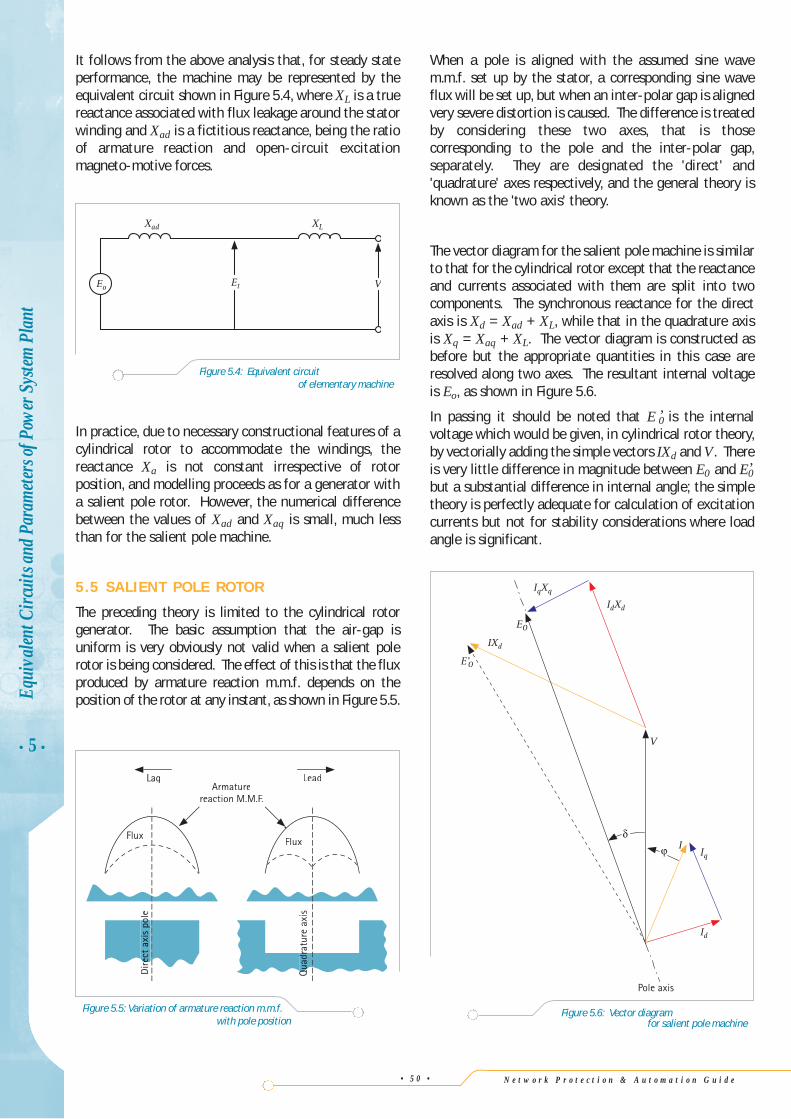
The preceding theory is limited to the cylindrical rotorgenerator. The basic assumption that the air-gap isuniform is very obviously not valid when a salient polerotor is being considered. The effect of this is that the fluxproduced by armature reaction m.m.f. depends on theposition of the rotor at any instant, as shown in Figure 5.5.

LagArmature

reaction M.M.F.

Lead

FluxFlux

Qu

ratu

reax

isQ

uadr

Dire

ole

rect

axis

po

N e t w o r k P r o t e c t i o n & A u t o m a t i o n G u i d e

When a pole is aligned with the assumed sine wavem.m.f. set up by the stator, a corresponding sine waveflux will be set up, but when an inter-polar gap is alignedvery severe distortion is caused. The difference is treatedby considering these two axes, that is thosecorresponding to the pole and the inter-polar gap,separately. They are designated the 'direct' and'quadrature' axes respectively, and the general theory isknown as the 'two axis' theory.

The vector diagram for the salient pole machine is similarto that for the cylindrical rotor except that the reactanceand currents associated with them are split into twocomponents. The synchronous reactance for the directaxis is Xd = Xad + XL, while that in the quadrature axisis Xq = Xaq + XL. The vector diagram is constructed asbefore but the appropriate quantities in this case areresolved along two axes. The resultant internal voltageis Eo, as shown in Figure 5.6.

In passing it should be noted that E ’0 is the internalvoltage which would be given, in cylindrical rotor theory,by vectorially adding the simple vectors IXd and V. Thereis very little difference in magnitude between E0 and E ’0but a substantial difference in internal angle; the simpletheory is perfectly adequate for calculation of excitationcurrents but not for stability considerations where loadangle is significant.

• 5 •

Equi

valen

t Circ

uits

and P

aram

eters

ofPo

wer

Sys

tem P

lant

• 5 0 •

Figure 5.5: Variation of armature reaction m.m.f.with pole position

V

Id

Iq

IdXd

IqXq

EO

IXd

E 'O

I

Pole axis

Figure 5.6: Vector diagram for salient pole machine

Figure 5.4: Equivalent circuit of elementary machine

Xad XL

Et VEo

N e t w o r k P r o t e c t i o n & A u t o m a t i o n G u i d e • 5 1 •

5.6 TRANSIENT ANALYSIS

For normal changes in load conditions, steady statetheory is perfectly adequate. However, there areoccasions when almost instantaneous changes areinvolved, such as faults or switching operations. Whenthis happens new factors are introduced within themachine and to represent these adequately acorresponding new set of machine characteristics isrequired.

The generally accepted and most simple way toappreciate the meaning and derivation of thesecharacteristics is to consider a sudden three-phase shortcircuit applied to a machine initially running on opencircuit and excited to normal voltage E0.

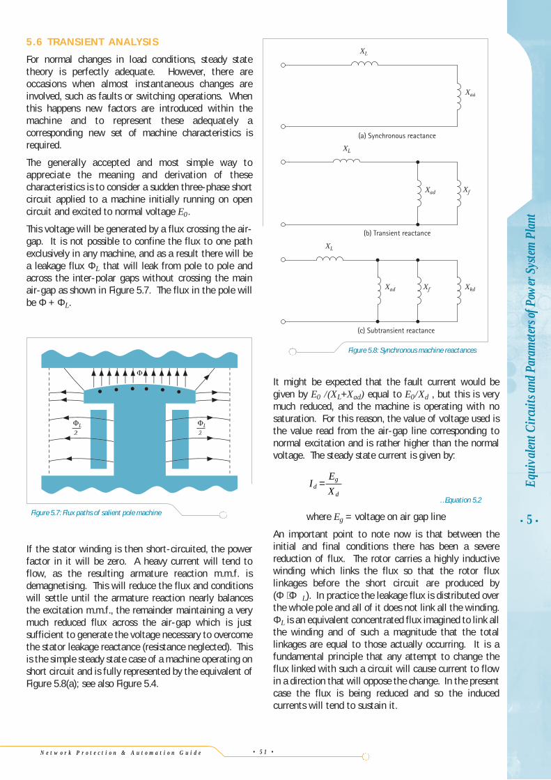
This voltage will be generated by a flux crossing the air-gap. It is not possible to confine the flux to one pathexclusively in any machine, and as a result there will bea leakage flux ΦL that will leak from pole to pole andacross the inter-polar gaps without crossing the mainair-gap as shown in Figure 5.7. The flux in the pole willbe Φ + ΦL.

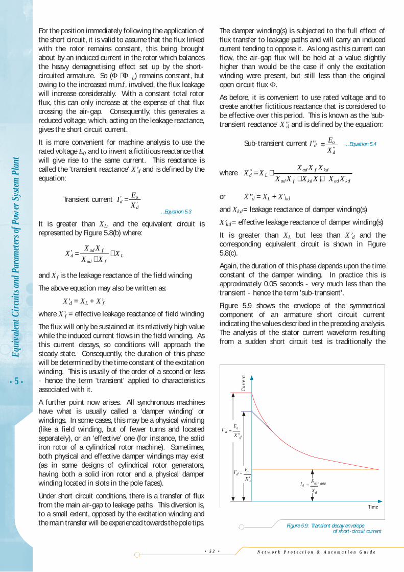
If the stator winding is then short-circuited, the powerfactor in it will be zero. A heavy current will tend toflow, as the resulting armature reaction m.m.f. isdemagnetising. This will reduce the flux and conditionswill settle until the armature reaction nearly balancesthe excitation m.m.f., the remainder maintaining a verymuch reduced flux across the air-gap which is justsufficient to generate the voltage necessary to overcomethe stator leakage reactance (resistance neglected). Thisis the simple steady state case of a machine operating onshort circuit and is fully represented by the equivalent ofFigure 5.8(a); see also Figure 5.4.

It might be expected that the fault current would begiven by E0 /(XL+Xad) equal to E0/Xd , but this is verymuch reduced, and the machine is operating with nosaturation. For this reason, the value of voltage used isthe value read from the air-gap line corresponding tonormal excitation and is rather higher than the normalvoltage. The steady state current is given by:

…Equation 5.2

where Eg = voltage on air gap line

An important point to note now is that between theinitial and final conditions there has been a severereduction of flux. The rotor carries a highly inductivewinding which links the flux so that the rotor fluxlinkages before the short circuit are produced by(Φ + ΦL). In practice the leakage flux is distributed overthe whole pole and all of it does not link all the winding.ΦL is an equivalent concentrated flux imagined to link allthe winding and of such a magnitude that the totallinkages are equal to those actually occurring. It is afundamental principle that any attempt to change theflux linked with such a circuit will cause current to flowin a direction that will oppose the change. In the presentcase the flux is being reduced and so the inducedcurrents will tend to sustain it.

IEXd

g

d

=

• 5 •Eq

uiva

lent C

ircui

ts an

d Par

amete

rs of

Pow

er S

ystem

Pla

nt

2L

2L

Figure 5.7: Flux paths of salient pole machine

Xad

Xad

Xad

Xf

XL

XL

XL

Xf

Xkd

(c) Subtransient reactance

(b) Transient reactance

(a) Synchronous reactance

Figure 5.8: Synchronous machine reactances

N e t w o r k P r o t e c t i o n & A u t o m a t i o n G u i d e

For the position immediately following the application ofthe short circuit, it is valid to assume that the flux linkedwith the rotor remains constant, this being broughtabout by an induced current in the rotor which balancesthe heavy demagnetising effect set up by the short-circuited armature. So (Φ + ΦL) remains constant, butowing to the increased m.m.f. involved, the flux leakagewill increase considerably. With a constant total rotorflux, this can only increase at the expense of that fluxcrossing the air-gap. Consequently, this generates areduced voltage, which, acting on the leakage reactance,gives the short circuit current.

It is more convenient for machine analysis to use therated voltage E0 and to invent a fictitious reactance thatwill give rise to the same current. This reactance iscalled the 'transient reactance' X’d and is defined by theequation:

Transient current

…Equation 5.3

It is greater than XL, and the equivalent circuit isrepresented by Figure 5.8(b) where:

and Xf is the leakage reactance of the field winding

The above equation may also be written as:

X’d = XL + X’f

where X’f = effective leakage reactance of field winding

The flux will only be sustained at its relatively high valuewhile the induced current flows in the field winding. Asthis current decays, so conditions will approach thesteady state. Consequently, the duration of this phasewill be determined by the time constant of the excitationwinding. This is usually of the order of a second or less- hence the term 'transient' applied to characteristicsassociated with it.

A further point now arises. All synchronous machineshave what is usually called a ‘damper winding’ orwindings. In some cases, this may be a physical winding(like a field winding, but of fewer turns and locatedseparately), or an ‘effective’ one (for instance, the solidiron rotor of a cylindrical rotor machine). Sometimes,both physical and effective damper windings may exist(as in some designs of cylindrical rotor generators,having both a solid iron rotor and a physical damperwinding located in slots in the pole faces).

Under short circuit conditions, there is a transfer of fluxfrom the main air-gap to leakage paths. This diversion is,to a small extent, opposed by the excitation winding andthe main transfer will be experienced towards the pole tips.

XX X

X XXd

ad f

ad fL' =

++

I EX

do

d

''

=

The damper winding(s) is subjected to the full effect offlux transfer to leakage paths and will carry an inducedcurrent tending to oppose it. As long as this current canflow, the air-gap flux will be held at a value slightlyhigher than would be the case if only the excitationwinding were present, but still less than the originalopen circuit flux Φ.

As before, it is convenient to use rated voltage and tocreate another fictitious reactance that is considered tobe effective over this period. This is known as the 'sub-transient reactance' X ’’d and is defined by the equation:

Sub-transient current I ’’d …Equation 5.4

where

or X’’d = XL + X’kd

and Xkd= leakage reactance of damper winding(s)

X’kd= effective leakage reactance of damper winding(s)

It is greater than XL but less than X ’d and thecorresponding equivalent circuit is shown in Figure5.8(c).

Again, the duration of this phase depends upon the timeconstant of the damper winding. In practice this isapproximately 0.05 seconds - very much less than thetransient - hence the term 'sub-transient'.

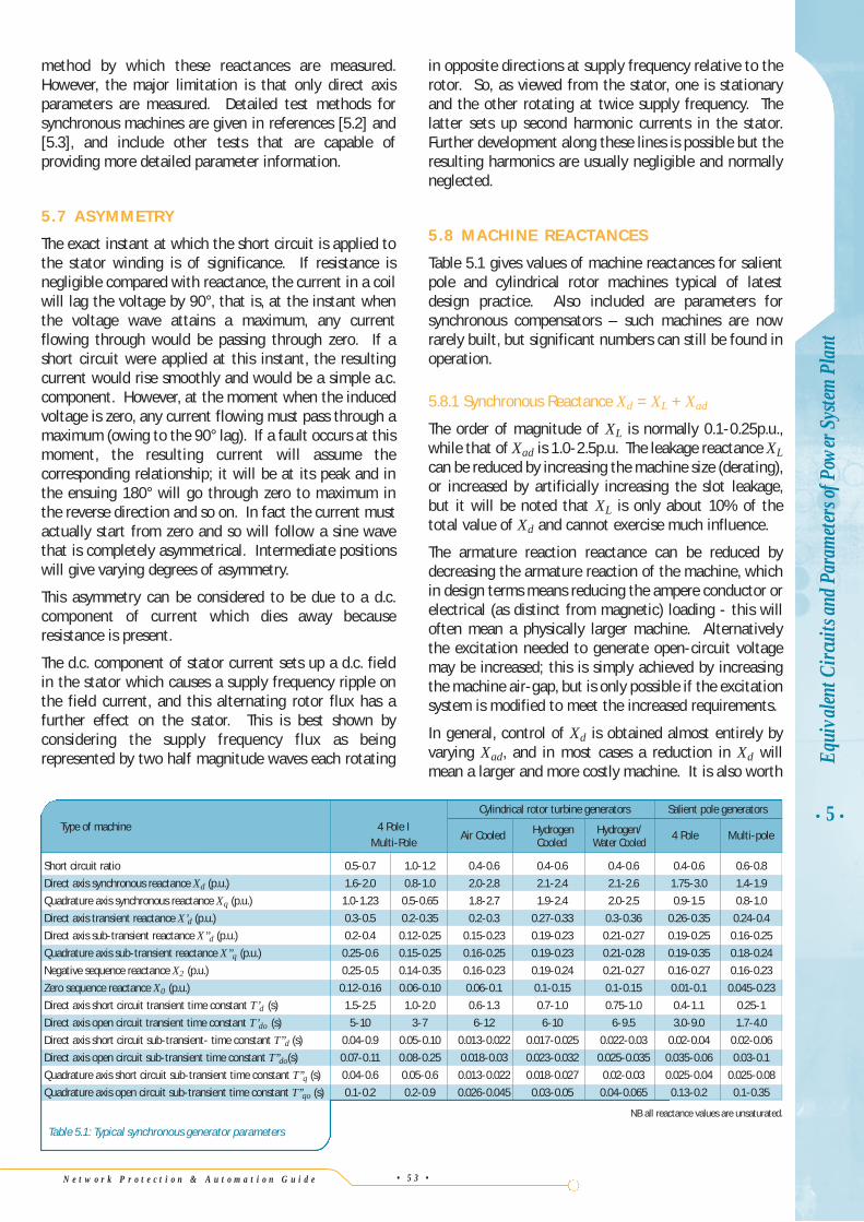
Figure 5.9 shows the envelope of the symmetricalcomponent of an armature short circuit currentindicating the values described in the preceding analysis.The analysis of the stator current waveform resultingfrom a sudden short circuit test is traditionally the

X XX X X

X X X X X Xd Lad f kd

ad f kd f ad kd

'' = ++ +

= EX

o

d''

• 5 •

Equi

valen

t Circ

uits

and P

aram

eters

ofPo

wer

Sys

tem P

lant

• 5 2 •

Curr

ent

Time

EoI''dX ''d

=

EoI 'dX 'd

=

Eair gapIdIXdX

=

Figure 5.9: Transient decay envelopeof short-circuit current

N e t w o r k P r o t e c t i o n & A u t o m a t i o n G u i d e

method by which these reactances are measured.However, the major limitation is that only direct axisparameters are measured. Detailed test methods forsynchronous machines are given in references [5.2] and[5.3], and include other tests that are capable ofproviding more detailed parameter information.

5.7 ASYMMETRY

The exact instant at which the short circuit is applied tothe stator winding is of significance. If resistance isnegligible compared with reactance, the current in a coilwill lag the voltage by 90°, that is, at the instant whenthe voltage wave attains a maximum, any currentflowing through would be passing through zero. If ashort circuit were applied at this instant, the resultingcurrent would rise smoothly and would be a simple a.c.component. However, at the moment when the inducedvoltage is zero, any current flowing must pass through amaximum (owing to the 90° lag). If a fault occurs at thismoment, the resulting current will assume thecorresponding relationship; it will be at its peak and inthe ensuing 180° will go through zero to maximum inthe reverse direction and so on. In fact the current mustactually start from zero and so will follow a sine wavethat is completely asymmetrical. Intermediate positionswill give varying degrees of asymmetry.

This asymmetry can be considered to be due to a d.c.component of current which dies away becauseresistance is present.

The d.c. component of stator current sets up a d.c. fieldin the stator which causes a supply frequency ripple onthe field current, and this alternating rotor flux has afurther effect on the stator. This is best shown byconsidering the supply frequency flux as beingrepresented by two half magnitude waves each rotating

in opposite directions at supply frequency relative to therotor. So, as viewed from the stator, one is stationaryand the other rotating at twice supply frequency. Thelatter sets up second harmonic currents in the stator.Further development along these lines is possible but theresulting harmonics are usually negligible and normallyneglected.

5.8 MACHINE REACTANCES

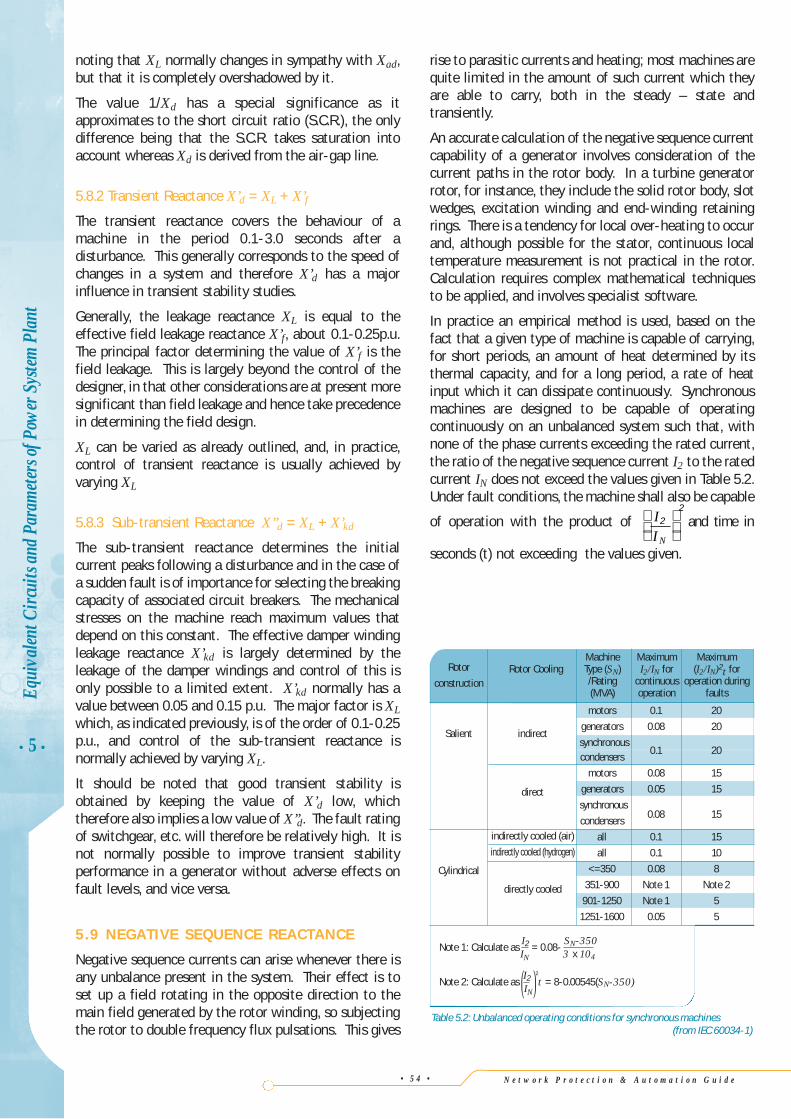
Table 5.1 gives values of machine reactances for salientpole and cylindrical rotor machines typical of latestdesign practice. Also included are parameters forsynchronous compensators – such machines are nowrarely built, but significant numbers can still be found inoperation.

5.8.1 Synchronous Reactance Xd = XL + Xad

The order of magnitude of XL is normally 0.1-0.25p.u.,while that of Xad is 1.0-2.5p.u. The leakage reactance XLcan be reduced by increasing the machine size (derating),or increased by artificially increasing the slot leakage,but it will be noted that XL is only about 10% of thetotal value of Xd and cannot exercise much influence.

The armature reaction reactance can be reduced bydecreasing the armature reaction of the machine, whichin design terms means reducing the ampere conductor orelectrical (as distinct from magnetic) loading - this willoften mean a physically larger machine. Alternativelythe excitation needed to generate open-circuit voltagemay be increased; this is simply achieved by increasingthe machine air-gap, but is only possible if the excitationsystem is modified to meet the increased requirements.

In general, control of Xd is obtained almost entirely byvarying Xad, and in most cases a reduction in Xd willmean a larger and more costly machine. It is also worth

• 5 •Eq

uiva

lent C

ircui

ts an

d Par

amete

rs of

Pow

er S

ystem

Pla

nt

• 5 3 •

Table 5.1: Typical synchronous generator parameters

Type of machine

Cylindrical rotor turbine generators Salient pole generators

4 Pole IAir Cooled Hydrogen Hydrogen/ 4 Pole Multi-pole

Multi-Pole Cooled Water Cooled

Short circuit ratio 0.5-0.7 1.0-1.2 0.4-0.6 0.4-0.6 0.4-0.6 0.4-0.6 0.6-0.8

Direct axis synchronous reactance Xd (p.u.) 1.6-2.0 0.8-1.0 2.0-2.8 2.1-2.4 2.1-2.6 1.75-3.0 1.4-1.9

Quadrature axis synchronous reactance Xq (p.u.) 1.0-1.23 0.5-0.65 1.8-2.7 1.9-2.4 2.0-2.5 0.9-1.5 0.8-1.0

Direct axis transient reactance X’d (p.u.) 0.3-0.5 0.2-0.35 0.2-0.3 0.27-0.33 0.3-0.36 0.26-0.35 0.24-0.4

Direct axis sub-transient reactance X’’d (p.u.) 0.2-0.4 0.12-0.25 0.15-0.23 0.19-0.23 0.21-0.27 0.19-0.25 0.16-0.25

Quadrature axis sub-transient reactance X’’q (p.u.) 0.25-0.6 0.15-0.25 0.16-0.25 0.19-0.23 0.21-0.28 0.19-0.35 0.18-0.24

Negative sequence reactance X2 (p.u.) 0.25-0.5 0.14-0.35 0.16-0.23 0.19-0.24 0.21-0.27 0.16-0.27 0.16-0.23

Zero sequence reactance X0 (p.u.) 0.12-0.16 0.06-0.10 0.06-0.1 0.1-0.15 0.1-0.15 0.01-0.1 0.045-0.23

Direct axis short circuit transient time constant T’d (s) 1.5-2.5 1.0-2.0 0.6-1.3 0.7-1.0 0.75-1.0 0.4-1.1 0.25-1

Direct axis open circuit transient time constant T’do (s) 5-10 3-7 6-12 6-10 6-9.5 3.0-9.0 1.7-4.0

Direct axis short circuit sub-transient- time constant T’’d (s) 0.04-0.9 0.05-0.10 0.013-0.022 0.017-0.025 0.022-0.03 0.02-0.04 0.02-0.06

Direct axis open circuit sub-transient time constant T’’do(s) 0.07-0.11 0.08-0.25 0.018-0.03 0.023-0.032 0.025-0.035 0.035-0.06 0.03-0.1

Quadrature axis short circuit sub-transient time constant T’’q (s) 0.04-0.6 0.05-0.6 0.013-0.022 0.018-0.027 0.02-0.03 0.025-0.04 0.025-0.08

Quadrature axis open circuit sub-transient time constant T’’qo (s) 0.1-0.2 0.2-0.9 0.026-0.045 0.03-0.05 0.04-0.065 0.13-0.2 0.1-0.35

NB all reactance values are unsaturated.

noting that XL normally changes in sympathy with Xad,but that it is completely overshadowed by it.

The value 1/Xd has a special significance as itapproximates to the short circuit ratio (S.C.R.), the onlydifference being that the S.C.R. takes saturation intoaccount whereas Xd is derived from the air-gap line.

5.8.2 Transient Reactance X’d = XL + X’f

The transient reactance covers the behaviour of amachine in the period 0.1-3.0 seconds after adisturbance. This generally corresponds to the speed ofchanges in a system and therefore X’d has a majorinfluence in transient stability studies.

Generally, the leakage reactance XL is equal to theeffective field leakage reactance X’f, about 0.1-0.25p.u.The principal factor determining the value of X’f is thefield leakage. This is largely beyond the control of thedesigner, in that other considerations are at present moresignificant than field leakage and hence take precedencein determining the field design.

XL can be varied as already outlined, and, in practice,control of transient reactance is usually achieved byvarying XL

5.8.3 Sub-transient Reactance X’’d = XL + X’kd

The sub-transient reactance determines the initialcurrent peaks following a disturbance and in the case ofa sudden fault is of importance for selecting the breakingcapacity of associated circuit breakers. The mechanicalstresses on the machine reach maximum values thatdepend on this constant. The effective damper windingleakage reactance X’kd is largely determined by theleakage of the damper windings and control of this isonly possible to a limited extent. X’kd normally has avalue between 0.05 and 0.15 p.u. The major factor is XLwhich, as indicated previously, is of the order of 0.1-0.25p.u., and control of the sub-transient reactance isnormally achieved by varying XL.

It should be noted that good transient stability isobtained by keeping the value of X’d low, whichtherefore also implies a low value of X’’d. The fault ratingof switchgear, etc. will therefore be relatively high. It isnot normally possible to improve transient stabilityperformance in a generator without adverse effects onfault levels, and vice versa.

5.9 NEGATIVE SEQUENCE REACTANCE

Negative sequence currents can arise whenever there isany unbalance present in the system. Their effect is toset up a field rotating in the opposite direction to themain field generated by the rotor winding, so subjectingthe rotor to double frequency flux pulsations. This gives

rise to parasitic currents and heating; most machines arequite limited in the amount of such current which theyare able to carry, both in the steady – state andtransiently.

An accurate calculation of the negative sequence currentcapability of a generator involves consideration of thecurrent paths in the rotor body. In a turbine generatorrotor, for instance, they include the solid rotor body, slotwedges, excitation winding and end-winding retainingrings. There is a tendency for local over-heating to occurand, although possible for the stator, continuous localtemperature measurement is not practical in the rotor.Calculation requires complex mathematical techniquesto be applied, and involves specialist software.

In practice an empirical method is used, based on thefact that a given type of machine is capable of carrying,for short periods, an amount of heat determined by itsthermal capacity, and for a long period, a rate of heatinput which it can dissipate continuously. Synchronousmachines are designed to be capable of operatingcontinuously on an unbalanced system such that, withnone of the phase currents exceeding the rated current,the ratio of the negative sequence current I2 to the ratedcurrent IN does not exceed the values given in Table 5.2.Under fault conditions, the machine shall also be capable

of operation with the product of and time in

seconds (t) not exceeding the values given.

II N

22

• 5 •

Equi

valen

t Circ

uits

and P

aram

eters

ofPo

wer

Sys

tem P

lant

motors 0.1 20

generators 0.08 20

synchronouscondensers

0.1 20

motors 0.08 15

generators 0.05 15

synchronous

condensers0.08 15

all 0.1 15

all 0.1 10

<=350 0.08 8

351-900 Note 1 Note 2

901-1250 Note 1 5

1251-1600 0.05 5

Machine Maximum MaximumRotor Cooling Type (SN) I2/IN for (I2/IN)2t for

/Rating continuous operation during(MVA) operation faults

indirect

direct

indirectly cooled (air)

indirectly cooled (hydrogen)

directly cooled

Salient

Cylindrical

Note 1: Calculate asI2 = 0.08-

SN-350IN 3 x 104

Note 2: Calculate as (I2 )2t = 8-0.00545(SN-350)IN

Table 5.2: Unbalanced operating conditions for synchronous machines(from IEC 60034-1)

N e t w o r k P r o t e c t i o n & A u t o m a t i o n G u i d e• 5 4 •

Rotor

construction

N e t w o r k P r o t e c t i o n & A u t o m a t i o n G u i d e • 5 5 •

5.10 ZERO SEQUENCE REACTANCE

If a machine is operating with an earthed neutral, asystem earth fault will give rise to zero sequencecurrents in the machine. This reactance represents themachine's contribution to the total impedance offered tothese currents. In practice it is generally low and oftenoutweighed by other impedances present in the circuit.

5.11 DIRECT AND QUADRATURE AXIS VALUES

The transient reactance is associated with the fieldwinding and since on salient pole machines this isconcentrated on the direct axis, there is nocorresponding quadrature axis value. The value ofreactance applicable in the quadrature axis is thesynchronous reactance, that is, X’q = Xq.

The damper winding (or its equivalent) is more widelyspread and hence the sub-transient reactance associatedwith this has a definite quadrature axis value X”q, whichdiffers significantly in many generators from X”d.

5.12 EFFECT OF SATURATIONON MACHINE REACTANCES

In general, any electrical machine is designed to avoidsevere saturation of its magnetic circuit. However, it isnot economically possible to operate at such low fluxdensities as to reduce saturation to negligibleproportions, and in practice a moderate degree ofsaturation is accepted.

Since the armature reaction reactance Xad is a ratioATar /ATe it is evident that ATe will not vary in a linearmanner for different voltages, while ATar will remainunchanged. The value of Xad will vary with the degree ofsaturation present in the machine, and for extremeaccuracy should be determined for the particularconditions involved in any calculation.

All the other reactances, namely XL , X’d and X’’d aretrue reactances and actually arise from flux leakage.Much of this leakage occurs in the iron parts of themachines and hence must be affected by saturation. Fora given set of conditions, the leakage flux exists as aresult of the net m.m.f. which causes it. If the ironcircuit is unsaturated its reactance is low and leakageflux is easily established. If the circuits are highlysaturated the reverse is true and the leakage flux isrelatively lower, so the reactance under saturatedconditions is lower than when unsaturated.

Most calculation methods assume infinite ironpermeability and for this reason lead to somewhatidealised unsaturated reactance values. The recognitionof a finite and varying permeability makes a solutionextremely laborious and in practice a simple factor ofapproximately 0.9 is taken as representing the reductionin reactance arising from saturation.

It is necessary to distinguish which value of reactance isbeing measured when on test. The normal instantaneousshort circuit test carried out from rated open circuitvoltage gives a current that is usually several times fullload value, so that saturation is present and thereactance measured will be the saturated value. Thisvalue is also known as the 'rated voltage' value since it ismeasured by a short circuit applied with the machineexcited to rated voltage.

In some cases, if it is wished to avoid the severemechanical strain to which a machine is subjected bysuch a direct short circuit, the test may be made from asuitably reduced voltage so that the initial current isapproximately full load value. Saturation is very muchreduced and the reactance values measured are virtuallyunsaturated values. They are also known as 'ratedcurrent' values, for obvious reasons.

5.13 TRANSFORMERS

A transformer may be replaced in a power system by anequivalent circuit representing the self-impedance of,and the mutual coupling between, the windings. A two-winding transformer can be simply represented as a 'T'network in which the cross member is the short-circuitimpedance, and the column the excitation impedance. Itis rarely necessary in fault studies to consider excitationimpedance as this is usually many times the magnitudeof the short-circuit impedance. With these simplifyingassumptions a three-winding transformer becomes a starof three impedances and a four-winding transformer amesh of six impedances.

The impedances of a transformer, in common with otherplant, can be given in ohms and qualified by a basevoltage, or in per unit or percentage terms and qualifiedby a base MVA. Care should be taken with multi-winding transformers to refer all impedances to acommon base MVA or to state the base on which each isgiven. The impedances of static apparatus areindependent of the phase sequence of the appliedvoltage; in consequence, transformer negative sequenceand positive sequence impedances are identical. Indetermining the impedance to zero phase sequencecurrents, account must be taken of the windingconnections, earthing, and, in some cases, theconstruction type. The existence of a path for zerosequence currents implies a fault to earth and a flow ofbalancing currents in the windings of the transformer.

Practical three-phase transformers may have a phaseshift between primary and secondary windingsdepending on the connections of the windings – delta orstar. The phase shift that occurs is generally of nosignificance in fault level calculations as all phases areshifted equally. It is therefore ignored. It is normal tofind delta-star transformers at the transmitting end of a

• 5 •Eq

uiva

lent C

ircui

ts an

d Par

amete

rs of

Pow

er S

ystem

Pla

nt

N e t w o r k P r o t e c t i o n & A u t o m a t i o n G u i d e

transmission system and in distribution systems for thefollowing reasons:

a. at the transmitting end, a higher step-up voltageratio is possible than with other windingarrangements, while the insulation to ground of thestar secondary winding does not increase by thesame ratio

b. in distribution systems, the star winding allows aneutral connection to be made, which may beimportant in considering system earthingarrangements

c. the delta winding allows circulation of zerosequence currents within the delta, thuspreventing transmission of these from thesecondary (star) winding into the primary circuit.This simplifies protection considerations

5.14 TRANSFORMER POSIT IVE SEQUENCE EQUIVALENT CIRCUITS

The transformer is a relatively simple device. However,the equivalent circuits for fault calculations need notnecessarily be quite so simple, especially where earthfaults are concerned. The following two sections discussthe equivalent circuits of various types of transformers.

5.14.1 Two-winding Transformers

The two-winding transformer has four terminals, but inmost system problems, two-terminal or three-terminalequivalent circuits as shown in Figure 5.10 can representit. In Figure 5.10(a), terminals A' and B' are assumed tobe at the same potential. Hence if the per unit self-impedances of the windings are Z11 and Z22 respectivelyand the mutual impedance between them Z12, the

transformer may be represented by Figure 5.10(b). Thecircuit in Figure 5.10(b) is similar to that shown in Figure3.14(a), and can therefore be replaced by an equivalent'T ' as shown in Figure 5.10(c) where:

…Equation 5.5

Z1 is described as the leakage impedance of winding AA'and Z2 the leakage impedance of winding BB'.

Impedance Z3 is the mutual impedance between thewindings, usually represented by XM, the magnetizingreactance paralleled with the hysteresis and eddy currentloops as shown in Figure 5.10(d).

If the secondary of the transformers is short-circuited,and Z3 is assumed to be large with respect to Z1 and Z2,then the short-circuit impedance viewed from theterminals AA’ is ZT = Z1 + Z2 and the transformer canbe replaced by a two-terminal equivalent circuit asshown in Figure 5.10(e).

The relative magnitudes of ZT and XM are of the order of10% and 2000% respectively. ZT and XM rarely have tobe considered together, so that the transformer may berepresented either as a series impedance or as anexcitation impedance, according to the problem beingstudied.

A typical power transformer is illustrated in Figure 5.11.

5.14.2 Three-winding Transformers

If excitation impedance is neglected the equivalentcircuit of a three-winding transformer may berepresented by a star of impedances, as shown in Figure5.12, where P, T and S are the primary, tertiary andsecondary windings respectively. The impedance of anyof these branches can be determined by considering theshort-circuit impedance between pairs of windings withthe third open.

Z Z Z

Z Z Z

Z Z

1 11 12

2 22 12

3 12

= −

= −

=

• 5 •

Equi

valen

t Circ

uits

and P

aram

eters

ofPo

wer

Sys

tem P

lant

• 5 6 •

Zero bus(d) 'π' equivalent circuit

Zero bus(b) Equivalent circuit of model

Zero bus(c) 'T' equivalent circuit

Zero bus(e) Equivalent circuit: secondary winding s/c

R jXM

B'

B' C '

B'B' A'

B'A'

A'

A'

B CA

A'

B

BA

BA

BA

AZT =Z1+Z2

Z1 =Z11-Z12 Z2=Z22-Z12

Z3=Z12

r1+jx1 r2+jx2

Z12Z11 Z22LoadE

(a) Model of transformer

~

Figure 5.10: Equivalent circuitsfor a two-winding transformer

Zero bus

S

P

T

Zt

Zs

Zp

Tertiary

Secondary

Primary

Figure 5.12: Equivalent circuitfor a three-winding transformer

N e t w o r k P r o t e c t i o n & A u t o m a t i o n G u i d e • 5 7 •

The exceptions to the general rule of neglectingmagnetising impedance occur when the transformer isstar/star and either or both neutrals are earthed. Inthese circumstances the transformer is connected to thezero bus through the magnetising impedance. Where athree-phase transformer bank is arranged withoutinterlinking magnetic flux (that is a three-phase shelltype, or three single-phase units) and provided there is apath for zero sequence currents, the zero sequenceimpedance is equal to the positive sequence impedance.In the case of three-phase core type units, the zerosequence fluxes produced by zero sequence currents canfind a high reluctance path, the effect being to reducethe zero sequence impedance to about 90% of thepositive sequence impedance.

However, in hand calculations, it is usual to ignore thisvariation and consider the positive and zero sequenceimpedances to be equal. It is common when usingsoftware to perform fault calculations to enter a value ofzero-sequence impedance in accordance with the aboveguidelines, if the manufacturer is unable to provide avalue.

• 5 •Eq

uiva

lentC

ircui

tsan

dPar

amete

rsof

Pow

erSy

stem

Plan

t

5.15 TRANSFORMER ZERO SEQUENCE EQUIVALENT CIRCUITS

The flow of zero sequence currents in a transformer isonly possible when the transformer forms part of aclosed loop for uni-directional currents and ampere-turnbalance is maintained between windings.

The positive sequence equivalent circuit is stillmaintained to represent the transformer, but now thereare certain conditions attached to its connection into theexternal circuit. The order of excitation impedance isvery much lower than for the positive sequence circuit;it will be roughly between 1 and 4 per unit, but still highenough to be neglected in most fault studies.

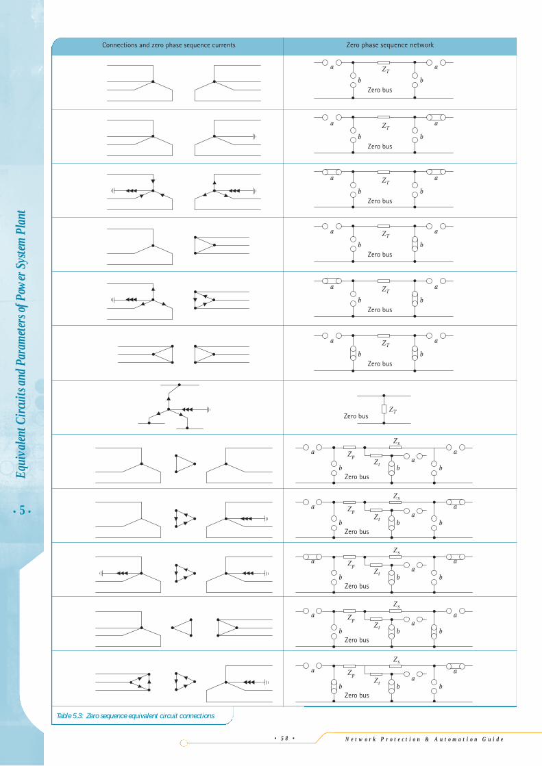
The mode of connection of a transformer to the externalcircuit is determined by taking account of each windingarrangement and its connection or otherwise to ground.If zero sequence currents can flow into and out of awinding, the winding terminal is connected to theexternal circuit (that is, link a is closed in Figure 5.13). Ifzero sequence currents can circulate in the windingwithout flowing in the external circuit, the windingterminal is connected directly to the zero bus (that is,link b is closed in Figure 5.13). Table 5.3 gives the zerosequence connections of some common two- and three-winding transformer arrangements applying the above rules.

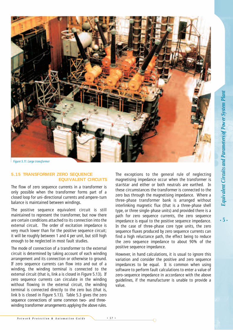
Figure 5.11: Large transformer

N e t w o r k P r o t e c t i o n & A u t o m a t i o n G u i d e

• 5 •

Equi

valen

t Circ

uits

and P

aram

eters

ofPo

wer

Sys

tem P

lant

• 5 8 •

Table 5.3: Zero sequence equivalent circuit connections

Zero busb

ZTa

b

a

Zero busb

ZTa

b

a

Zero busb

ZTa

b

a

Zero busb

ZTa

b

a

Zero busb

ZTa

b

a

Zero bus

Zero bus

b

ZT

ZT

ab b

a

b

a

Zero bus

Zt

Zs

Zp

ab b

a

b

a

Zero bus

Zt

Zs

Zp

ab b

a

b

a

Zero bus

Zt

Zs

Zp

ab b

a

b

a

Zero bus

Zt

Zs

Zp

ab b

a

b

a

Zero bus

Zt

Zs

Zp

a

b

a

Zero phase sequence networkConnections and zero phase sequence currents

N e t w o r k P r o t e c t i o n & A u t o m a t i o n G u i d e • 5 9 •

5.16 AUTO-TRANSFORMERS

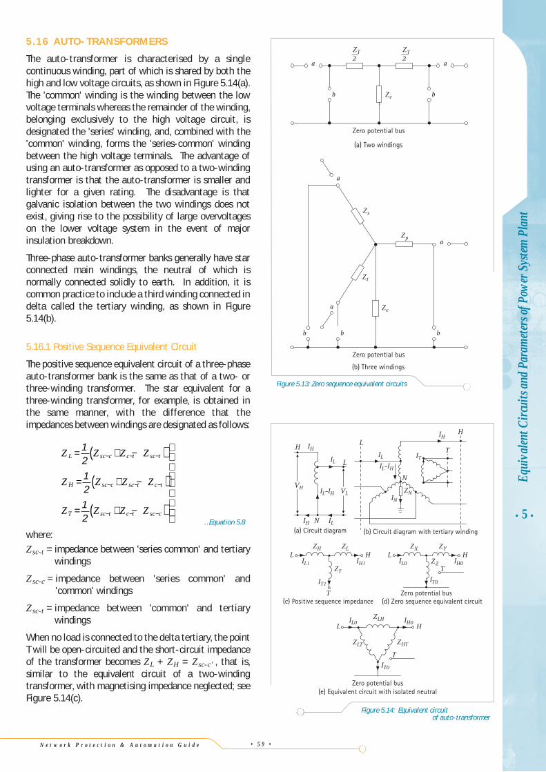
The auto-transformer is characterised by a singlecontinuous winding, part of which is shared by both thehigh and low voltage circuits, as shown in Figure 5.14(a).The 'common' winding is the winding between the lowvoltage terminals whereas the remainder of the winding,belonging exclusively to the high voltage circuit, isdesignated the 'series' winding, and, combined with the'common' winding, forms the 'series-common' windingbetween the high voltage terminals. The advantage ofusing an auto-transformer as opposed to a two-windingtransformer is that the auto-transformer is smaller andlighter for a given rating. The disadvantage is thatgalvanic isolation between the two windings does notexist, giving rise to the possibility of large overvoltageson the lower voltage system in the event of majorinsulation breakdown.

Three-phase auto-transformer banks generally have starconnected main windings, the neutral of which isnormally connected solidly to earth. In addition, it iscommon practice to include a third winding connected indelta called the tertiary winding, as shown in Figure5.14(b).

5.16.1 Positive Sequence Equivalent Circuit

The positive sequence equivalent circuit of a three-phaseauto-transformer bank is the same as that of a two- orthree-winding transformer. The star equivalent for athree-winding transformer, for example, is obtained inthe same manner, with the difference that theimpedances between windings are designated as follows:

…Equation 5.8

where:Zsc-t = impedance between 'series common' and tertiary

windings

Zsc-c = impedance between 'series common' and'common' windings

Zsc-t = impedance between 'common' and tertiarywindings

When no load is connected to the delta tertiary, the pointT will be open-circuited and the short-circuit impedanceof the transformer becomes ZL + ZH = Zsc-c’ , that is,similar to the equivalent circuit of a two-windingtransformer, with magnetising impedance neglected; seeFigure 5.14(c).

Z Z Z Z

Z Z Z Z

Z Z Z Z

L sc c c t sc t

H sc c sc t c t

T sc t c t sc c

= + −( )

= + −( )

= + −( )

− − −

− − −

− − −

12

12

12 • 5 •

Equi

valen

t Circ

uits

and P

aram

eters

ofPo

wer

Sys

tem P

lant

Zero potential bus

a

b

Ze

Zt

Zp

Zs

Ze

bb

a

a

(b) Three windings

(a) Two windings

Zero potential bus

b

aa

b

ZT2

ZT2

Figure 5.13: Zero sequence equivalent circuits

H

L

N

L

N

T

H

T

HL HL

T

Zero potential bus

Zero potential bus(e) Equivalent circuit with isolated neutral

L H

T

ZHT

ZLH

ZX

ZZ

ZYZH

IH IL

IL-IH

IL-IH

VLVH

IH

IH

ILIL IT

INZN

ZL

ZT

ZLT

IL0 IH0

IL0

IT0IT1

IL1 IH0IH1

IT0

(c) Positive sequence impedance (d) Zero sequence equivalent circuit

(a) Circuit diagram (b) Circuit diagram with tertiary winding

Figure 5.14: Equivalent circuitof auto-transformer

N e t w o r k P r o t e c t i o n & A u t o m a t i o n G u i d e

5.16.2 Zero Sequence Equivalent Circuit

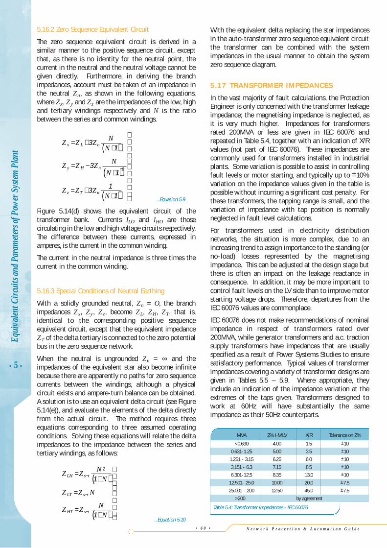
The zero sequence equivalent circuit is derived in asimilar manner to the positive sequence circuit, exceptthat, as there is no identity for the neutral point, thecurrent in the neutral and the neutral voltage cannot begiven directly. Furthermore, in deriving the branchimpedances, account must be taken of an impedance inthe neutral Zn, as shown in the following equations,where Zx, Zy and Zz are the impedances of the low, highand tertiary windings respectively and N is the ratiobetween the series and common windings.

…Equation 5.9

Figure 5.14(d) shows the equivalent circuit of thetransformer bank. Currents ILO and IHO are thosecirculating in the low and high voltage circuits respectively.The difference between these currents, expressed inamperes, is the current in the common winding.

The current in the neutral impedance is three times thecurrent in the common winding.

5.16.3 Special Conditions of Neutral Earthing

With a solidly grounded neutral, Zn = O, the branchimpedances Zx, Zy, Zz, become ZL, ZH, ZT, that is,identical to the corresponding positive sequenceequivalent circuit, except that the equivalent impedanceZT of the delta tertiary is connected to the zero potentialbus in the zero sequence network.

When the neutral is ungrounded Zn = ∞ and theimpedances of the equivalent star also become infinitebecause there are apparently no paths for zero sequencecurrents between the windings, although a physicalcircuit exists and ampere-turn balance can be obtained.A solution is to use an equivalent delta circuit (see Figure5.14(e)), and evaluate the elements of the delta directlyfrom the actual circuit. The method requires threeequations corresponding to three assumed operatingconditions. Solving these equations will relate the deltaimpedances to the impedance between the series andtertiary windings, as follows:

…Equation 5.10

Z Z NN

Z Z N

Z Z NN

LH s t

LT s t

HT s t

=+( )

=

=+( )

−

−

−

2

1

1

Z Z Z NN

Z Z Z N

N

Z Z ZN

x L n

y H n

z T n

= ++( )

= −+( )

= ++( )

31

31

3 11

2

With the equivalent delta replacing the star impedancesin the auto-transformer zero sequence equivalent circuitthe transformer can be combined with the systemimpedances in the usual manner to obtain the systemzero sequence diagram.

5.17 TRANSFORMER IMPEDANCES

In the vast majority of fault calculations, the ProtectionEngineer is only concerned with the transformer leakageimpedance; the magnetising impedance is neglected, asit is very much higher. Impedances for transformersrated 200MVA or less are given in IEC 60076 andrepeated in Table 5.4, together with an indication of X/Rvalues (not part of IEC 60076). These impedances arecommonly used for transformers installed in industrialplants. Some variation is possible to assist in controllingfault levels or motor starting, and typically up to ±10%variation on the impedance values given in the table ispossible without incurring a significant cost penalty. Forthese transformers, the tapping range is small, and thevariation of impedance with tap position is normallyneglected in fault level calculations.

For transformers used in electricity distributionnetworks, the situation is more complex, due to anincreasing trend to assign importance to the standing (orno-load) losses represented by the magnetisingimpedance. This can be adjusted at the design stage butthere is often an impact on the leakage reactance inconsequence. In addition, it may be more important tocontrol fault levels on the LV side than to improve motorstarting voltage drops. Therefore, departures from theIEC 60076 values are commonplace.

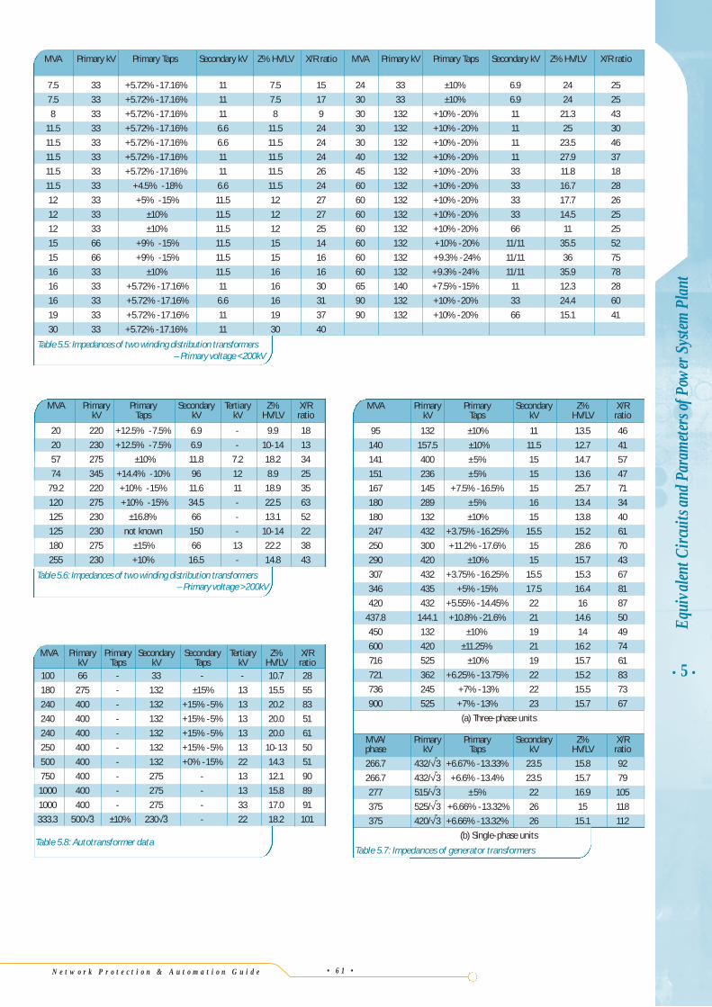
IEC 60076 does not make recommendations of nominalimpedance in respect of transformers rated over200MVA, while generator transformers and a.c. tractionsupply transformers have impedances that are usuallyspecified as a result of Power Systems Studies to ensuresatisfactory performance. Typical values of transformerimpedances covering a variety of transformer designs aregiven in Tables 5.5 – 5.9. Where appropriate, theyinclude an indication of the impedance variation at theextremes of the taps given. Transformers designed towork at 60Hz will have substantially the sameimpedance as their 50Hz counterparts.

• 5 •

Equi

valen

t Circ

uits

and P

aram

eters

ofPo

wer

Sys

tem P

lant

• 6 0 •

MVA Z% HV/LV X/R Tolerance on Z%

<0.630 4.00 1.5 ±10

0.631-1.25 5.00 3.5 ±10

1.251 - 3.15 6.25 6.0 ±10

3.151 - 6.3 7.15 8.5 ±10

6.301-12.5 8.35 13.0 ±10

12.501- 25.0 10.00 20.0 ±7.5

25.001 - 200 12.50 45.0 ±7.5

>200 by agreement

Table 5.4: Transformer impedances - IEC 60076

N e t w o r k P r o t e c t i o n & A u t o m a t i o n G u i d e • 6 1 •

• 5 •Eq

uiva

lent C

ircui

ts an

d Par

amete

rs of

Pow

er S

ystem

Pla

nt

MVA Primary kV Primary Taps Secondary kV Z% HV/LV X/R ratio MVA Primary kV Primary Taps Secondary kV Z% HV/LV X/R ratio

7.5 33 +5.72% -17.16% 11 7.5 15 24 33 ±10% 6.9 24 25

7.5 33 +5.72% -17.16% 11 7.5 17 30 33 ±10% 6.9 24 25

8 33 +5.72% -17.16% 11 8 9 30 132 +10% -20% 11 21.3 43

11.5 33 +5.72% -17.16% 6.6 11.5 24 30 132 +10% -20% 11 25 30

11.5 33 +5.72% -17.16% 6.6 11.5 24 30 132 +10% -20% 11 23.5 46

11.5 33 +5.72% -17.16% 11 11.5 24 40 132 +10% -20% 11 27.9 37

11.5 33 +5.72% -17.16% 11 11.5 26 45 132 +10% -20% 33 11.8 18

11.5 33 +4.5% -18% 6.6 11.5 24 60 132 +10% -20% 33 16.7 28

12 33 +5% -15% 11.5 12 27 60 132 +10% -20% 33 17.7 26

12 33 ±10% 11.5 12 27 60 132 +10% -20% 33 14.5 25

12 33 ±10% 11.5 12 25 60 132 +10% -20% 66 11 25

15 66 +9% -15% 11.5 15 14 60 132 +10% -20% 11/11 35.5 52

15 66 +9% -15% 11.5 15 16 60 132 +9.3% -24% 11/11 36 75

16 33 ±10% 11.5 16 16 60 132 +9.3% -24% 11/11 35.9 78

16 33 +5.72% -17.16% 11 16 30 65 140 +7.5% -15% 11 12.3 28

16 33 +5.72% -17.16% 6.6 16 31 90 132 +10% -20% 33 24.4 60

19 33 +5.72% -17.16% 11 19 37 90 132 +10% -20% 66 15.1 41

30 33 +5.72% -17.16% 11 30 40

MVA Primary Primary Secondary Tertiary Z% X/RkV Taps kV kV HV/LV ratio

20 220 +12.5% -7.5% 6.9 - 9.9 18

20 230 +12.5% -7.5% 6.9 - 10-14 13

57 275 ±10% 11.8 7.2 18.2 34

74 345 +14.4% -10% 96 12 8.9 25

79.2 220 +10% -15% 11.6 11 18.9 35

120 275 +10% -15% 34.5 - 22.5 63

125 230 ±16.8% 66 - 13.1 52

125 230 not known 150 - 10-14 22

180 275 ±15% 66 13 22.2 38

255 230 +10% 16.5 - 14.8 43

Table 5.6: Impedances of two winding distribution transformers– Primary voltage >200kV

MVA Primary Primary Secondary Z% X/RkV Taps kV HV/LV ratio

95 132 ±10% 11 13.5 46

140 157.5 ±10% 11.5 12.7 41

141 400 ±5% 15 14.7 57

151 236 ±5% 15 13.6 47

167 145 +7.5% -16.5% 15 25.7 71

180 289 ±5% 16 13.4 34

180 132 ±10% 15 13.8 40

247 432 +3.75% -16.25% 15.5 15.2 61

250 300 +11.2% -17.6% 15 28.6 70

290 420 ±10% 15 15.7 43

307 432 +3.75% -16.25% 15.5 15.3 67

346 435 +5% -15% 17.5 16.4 81

420 432 +5.55% -14.45% 22 16 87

437.8 144.1 +10.8% -21.6% 21 14.6 50

450 132 ±10% 19 14 49

600 420 ±11.25% 21 16.2 74

716 525 ±10% 19 15.7 61

721 362 +6.25% -13.75% 22 15.2 83

736 245 +7% -13% 22 15.5 73

900 525 +7% -13% 23 15.7 67

(a) Three-phase units

MVA/ Primary Primary Secondary Z% X/Rphase kV Taps kV HV/LV ratio

266.7 432/√-3 +6.67% -13.33% 23.5 15.8 92

266.7 432/√-3 +6.6% -13.4% 23.5 15.7 79

277 515/√-3 ±5% 22 16.9 105

375 525/√-3 +6.66% -13.32% 26 15 118

375 420/√-3 +6.66% -13.32% 26 15.1 112

(b) Single-phase units

Table 5.7: Impedances of generator transformers

Table 5.5: Impedances of two winding distribution transformers – Primary voltage <200kV

MVA Primary Primary Secondary Secondary Tertiary Z% X/RkV Taps kV Taps kV HV/LV ratio

100 66 - 33 - - 10.7 28

180 275 - 132 ±15% 13 15.5 55

240 400 - 132 +15% -5% 13 20.2 83

240 400 - 132 +15% -5% 13 20.0 51

240 400 - 132 +15% -5% 13 20.0 61

250 400 - 132 +15% -5% 13 10-13 50

500 400 - 132 +0% -15% 22 14.3 51

750 400 - 275 - 13 12.1 90

1000 400 - 275 - 13 15.8 89

1000 400 - 275 - 33 17.0 91

333.3 500√−3 ±10% 230√−3 - 22 18.2 101

Table 5.8: Autotransformer data

N e t w o r k P r o t e c t i o n & A u t o m a t i o n G u i d e

5.18 OVERHEAD L INES AND CABLES

In this section a description of common overhead linesand cable systems is given, together with tables of theirimportant characteristics. The formulae for calculatingthe characteristics are developed to give a basic idea ofthe factors involved, and to enable calculations to bemade for systems other than those tabulated.

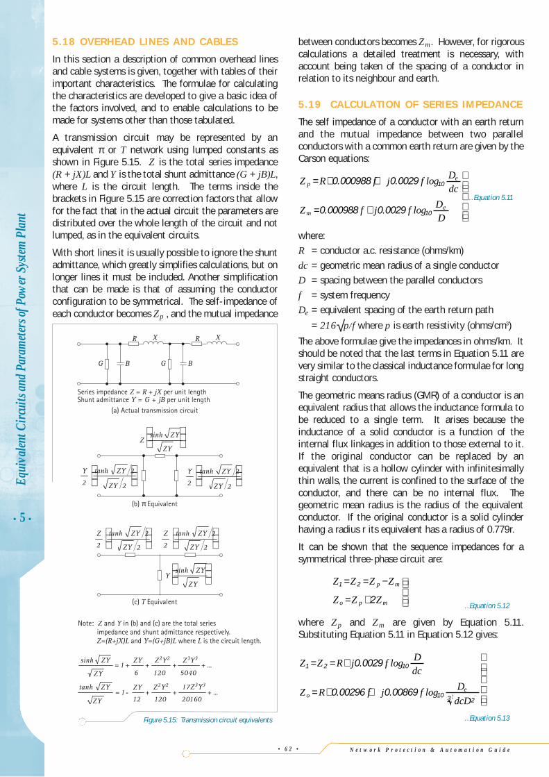
A transmission circuit may be represented by anequivalent π or T network using lumped constants asshown in Figure 5.15. Z is the total series impedance(R + jX)L and Y is the total shunt admittance (G + jB)L,where L is the circuit length. The terms inside thebrackets in Figure 5.15 are correction factors that allowfor the fact that in the actual circuit the parameters aredistributed over the whole length of the circuit and notlumped, as in the equivalent circuits.

With short lines it is usually possible to ignore the shuntadmittance, which greatly simplifies calculations, but onlonger lines it must be included. Another simplificationthat can be made is that of assuming the conductorconfiguration to be symmetrical. The self-impedance ofeach conductor becomes Zp , and the mutual impedance

between conductors becomes Zm. However, for rigorouscalculations a detailed treatment is necessary, withaccount being taken of the spacing of a conductor inrelation to its neighbour and earth.

5.19 CALCULATION OF SERIES IMPEDANCE

The self impedance of a conductor with an earth returnand the mutual impedance between two parallelconductors with a common earth return are given by theCarson equations:

…Equation 5.11

where:

R = conductor a.c. resistance (ohms/km)

dc = geometric mean radius of a single conductor

D = spacing between the parallel conductors

f = system frequency

De = equivalent spacing of the earth return path

= 216√p/f where p is earth resistivity (ohms/cm3)

The above formulae give the impedances in ohms/km. Itshould be noted that the last terms in Equation 5.11 arevery similar to the classical inductance formulae for longstraight conductors.

The geometric means radius (GMR) of a conductor is anequivalent radius that allows the inductance formula tobe reduced to a single term. It arises because theinductance of a solid conductor is a function of theinternal flux linkages in addition to those external to it.If the original conductor can be replaced by anequivalent that is a hollow cylinder with infinitesimallythin walls, the current is confined to the surface of theconductor, and there can be no internal flux. Thegeometric mean radius is the radius of the equivalentconductor. If the original conductor is a solid cylinderhaving a radius r its equivalent has a radius of 0.779r.

It can be shown that the sequence impedances for asymmetrical three-phase circuit are:

…Equation 5.12

where Zp and Zm are given by Equation 5.11.Substituting Equation 5.11 in Equation 5.12 gives:

…Equation 5.13

Z Z R j f Ddc

Z R f j f DdcD

oe

1 2 10

1023

0 0029

0 00296 0 00869

= = +

= + +

. log

. . log

Z Z Z Z

Z Z Z

p m

o p m

1 2

2

= = −

= +

Z R f j f Ddc

Z f j f DD

pe

me

= + +

= +

0 000988 0 0029

0 000988 0 0029

10

10

. . log

. . log

• 5 •

Equi

valen

t Circ

uits

and P

aram

eters

ofPo

wer

Sys

tem P

lant

• 6 2 •

(a) Actual transmission circuit

R XR X

BGBG

Series impedance Z = R + jX per unit lengthShunt admittance Y = G + jB per unit length

(b) π Equivalent

(c) T Equivalent

Note: Z and Y in (b) and (c) are the total series impedance and shunt admittance respectively.

Z=(R+jX)L and Y=(G+jB)L where L is the circuit length.

...5040120

Z2Y2

Z2Y2

Z3Y3

17Z3Y3

6

ZY

ZY

1ZY

ZY

ZY

ZY

sinh++++=

...2016012012

1tanh

+++-=

2

2

2 ZY

ZYtanhY 2

2

2 ZY

ZYtanhY

2

2

2 ZY

ZYtanhZ 2

2

2 ZY

ZYtanhZ

ZY

ZYsinhY

ZY

ZYsinhZ

Figure 5.15: Transmission circuit equivalents

N e t w o r k P r o t e c t i o n & A u t o m a t i o n G u i d e • 6 3 •

In the formula for Z0 the expression 3√dcD2 is the

geometric mean radius of the conductor group.Where the circuit is not symmetrical, the usual case,symmetry can be maintained by transposing theconductors so that each conductor is in each phaseposition for one third of the circuit length. If A, B and Care the spacings between conductors bc, ca and ab thenD in the above equations becomes the geometric meandistance between conductors, equal to 3√ABC.

Writing Dc = 3√dcD2, the sequence impedances inohms/km at 50Hz become:

…Equation 5.14

5.20 CALCULATION OF SHUNT IMPEDANCE

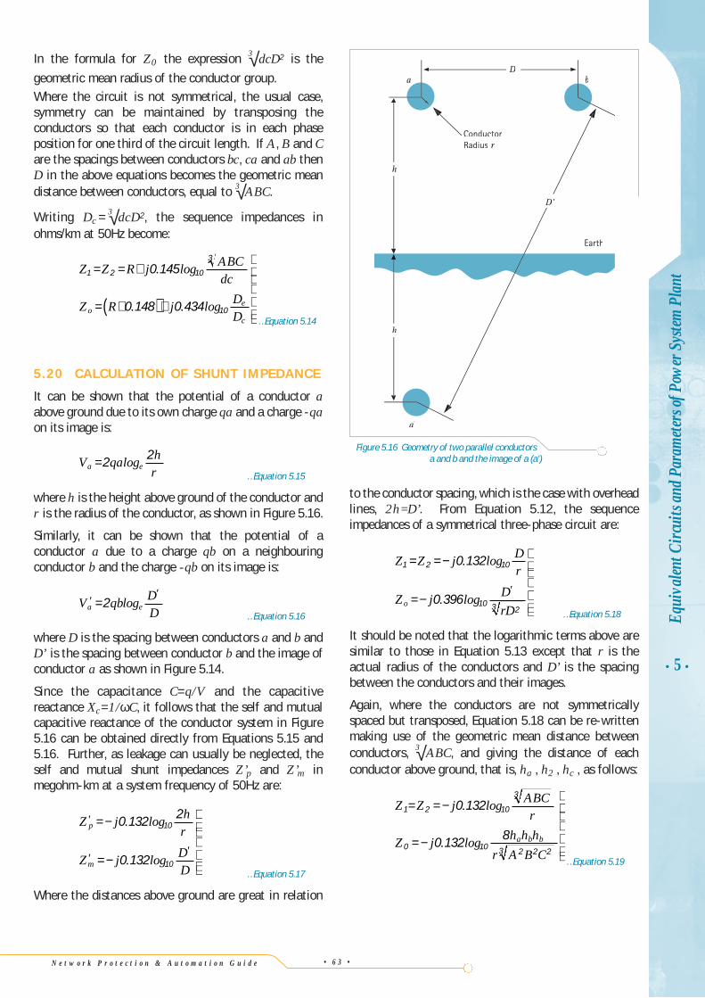
It can be shown that the potential of a conductor aabove ground due to its own charge qa and a charge -qaon its image is:

…Equation 5.15

where h is the height above ground of the conductor andr is the radius of the conductor, as shown in Figure 5.16.

Similarly, it can be shown that the potential of aconductor a due to a charge qb on a neighbouringconductor b and the charge -qb on its image is:

…Equation 5.16

where D is the spacing between conductors a and b andD’ is the spacing between conductor b and the image ofconductor a as shown in Figure 5.14.

Since the capacitance C=q/V and the capacitivereactance Xc=1/ωC, it follows that the self and mutualcapacitive reactance of the conductor system in Figure5.16 can be obtained directly from Equations 5.15 and5.16. Further, as leakage can usually be neglected, theself and mutual shunt impedances Z’p and Z’m inmegohm-km at a system frequency of 50Hz are:

…Equation 5.17

Where the distances above ground are great in relation

Z j hr

Z j DD

p

m

'

''

=−

=−

0 132 2

0 132

10

10

. log

. log

V qb DDa e''

=2 log

V qa hra e=2 2log

Z Z R j ABCdc

Z R j DDo

e

c

1 2 10

3

10

0 145

0 148 0 434

= = +

= +( )+

. log

. . log

to the conductor spacing, which is the case with overheadlines, 2h=D’. From Equation 5.12, the sequenceimpedances of a symmetrical three-phase circuit are:

…Equation 5.18

It should be noted that the logarithmic terms above aresimilar to those in Equation 5.13 except that r is theactual radius of the conductors and D’ is the spacingbetween the conductors and their images.

Again, where the conductors are not symmetricallyspaced but transposed, Equation 5.18 can be re-writtenmaking use of the geometric mean distance betweenconductors, 3√ABC, and giving the distance of eachconductor above ground, that is, ha , h2 , hc , as follows:

…Equation 5.19

Z Z j ABCr

Z j h h h

r A B Ca b b

1 2 10

3

0 10 2 2 23

0 132

0 132 8

= =−

=−

. log

. log

Z Z j Dr

Z j DrD

o

1 2 10

1023

0 132

0 396

= =−

=−

. log

. log'

• 5 •Eq

uiva

lent C

ircui

ts an

d Par

amete

rs of

Pow

er S

ystem

Pla

nt

Earth

a'

h

h

a b

D '

D

ConductorRadius r

Figure 5.16 Geometry of two parallel conductorsa and b and the image of a (a')

N e t w o r k P r o t e c t i o n & A u t o m a t i o n G u i d e

• 5 •

Equi

valen

t Circ

uits

and P

aram

eters

ofPo

wer

Sys

tem P

lant

• 6 4 •

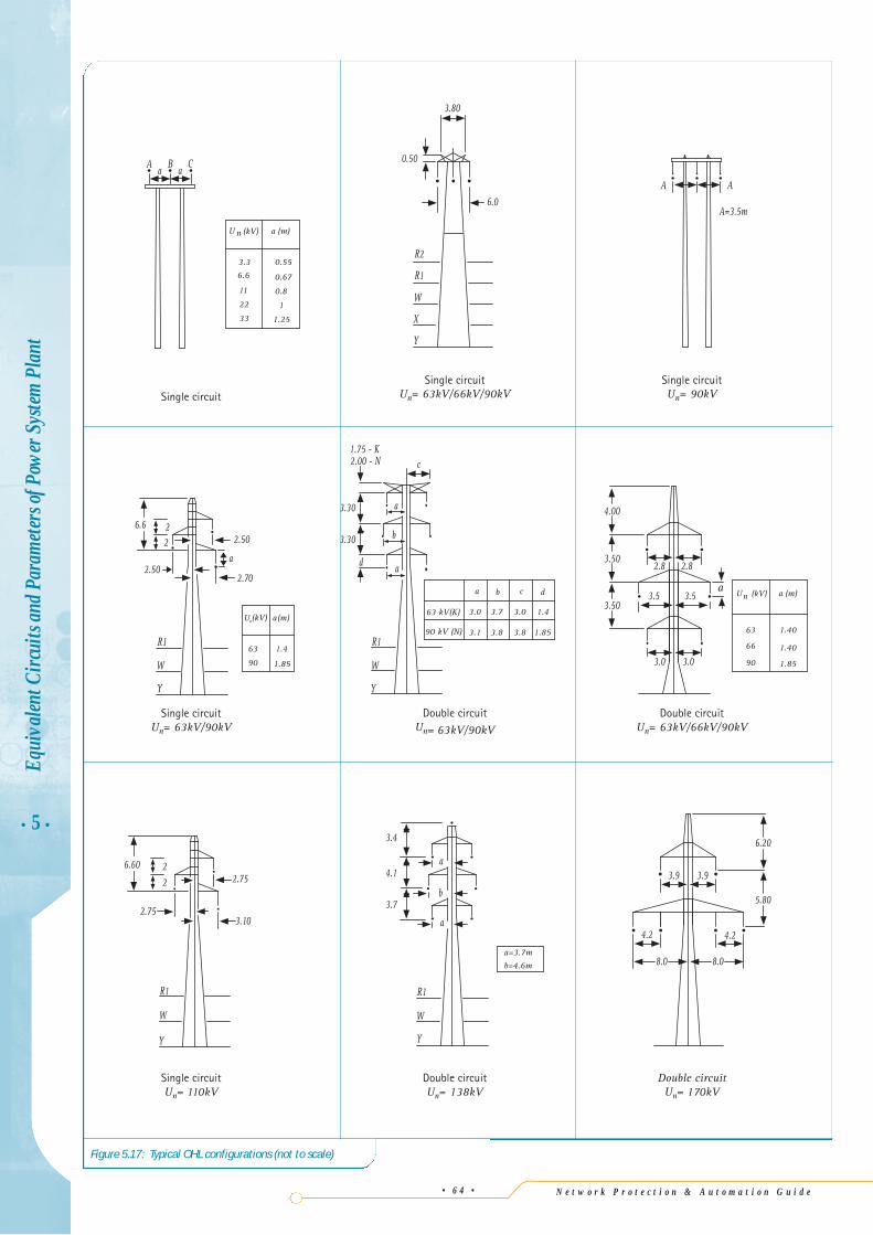
Figure 5.17: Typical OHL configurations (not to scale)

2.75

R1

Y

2.753.10

W

R1

Y

a

b

a

3.30

3.30

d

2.00 - N1.75 - K

c

W

a b c d

1.43.03.73.063 kV(K)

90 kV (N) 3.1 3.8 3.8 1.85

Y

W

R1

2.50

2.70

6.6

a2.50

Double circuitUn= 170kV

Double circuitUn= 138kV

Single circuitUn= 110kV

Single circuitUn= 63kV/90kV

Single circuitUn= 90kV

Double circuitUn= 63kV/90kV

Double circuitUn= 63kV/66kV/90kV

Single circuitUn= 63kV/66kV/90kVSingle circuit

3.93.9

4.24.2

5.80

6.20

Y

W

3.7

R1

a

b

4.1a

3.4

1.40

1.85

1.40

(m)

63

66

nU (kV) a

90

A=3.5m

AA

A CBa a

3.3

6.6

11

22

33

U n (kV)

1

1.25

0.55

0.8

0.67

a (m)

R1

Y

X

W

R2

6.0

0.50

3.80

2.8 2.8

8.08.0

3.5 3.5

3.0 3.0

3.50

3.50

4.00

a

90

63

(kV)nU

1.85

1.4

(m)a

22

6.60 22

a=3.7m

b=4.6m

N e t w o r k P r o t e c t i o n & A u t o m a t i o n G u i d e • 6 5 •

• 5 •Eq

uiva

lent C

ircui

ts an

d Par

amete

rs of

Pow

er S

ystem

Pla

nt

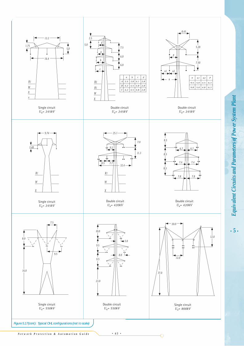
Figure 5.17(cont): Typical OHL configurations (not to scale)

W

R1

R2

b

a

5.0d

2.5

c6.0

6.0

7.5

X

W

X

R1

2.40

9.74

32.48.5

25.1

9.2

11.3

7.0

X

W

R1

7.7

5.0

8.0

9.5

10.0

9.5

23.0

12.0

7.4

8.5

7.8

7.4

6.7

7.8

6.7

8.5

8.5

n1n

9.8

9.5

5.0

5.0

n2 p

6.3

6.3

4.8

4.5n

n1

p

5.20

7.50

8.45

n2

12.0

37.0

20.00

0 0 0

0

Y

X

W

R1

16.4

12.2

1.755.0

9.5

7.5

16.0

8.0

2.8

2.8

d

3.5

a

4.2

cb

4.5

3.8

4.8

4.1A

4.84.54.2 2.8

B

C

Single circuitUn= 800kV

Double circuitUn= 550kV

Double circuitUn= 420kV

Double circuitUn= 420kV

Double circuitUn= 245kV

Double circuitUn= 245kV

Single circuitUn= 550kV

Single circuitUn= 245kV

Single circuitUn= 245kV

N e t w o r k P r o t e c t i o n & A u t o m a t i o n G u i d e

5.21 OVERHEAD L INE CIRCUITSWITH OR WITHOUT EARTH WIRES

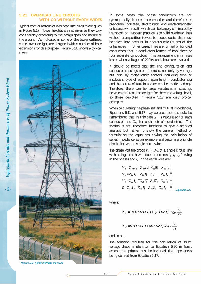
Typical configurations of overhead line circuits are givenin Figure 5.17. Tower heights are not given as they varyconsiderably according to the design span and nature ofthe ground. As indicated in some of the tower outlines,some tower designs are designed with a number of baseextensions for this purpose. Figure 5.18 shows a typicaltower.

In some cases, the phase conductors are notsymmetrically disposed to each other and therefore, aspreviously indicated, electrostatic and electromagneticunbalance will result, which can be largely eliminated bytransposition. Modern practice is to build overhead lineswithout transposition towers to reduce costs; this mustbe taken into account in rigorous calculations of theunbalances. In other cases, lines are formed of bundledconductors, that is conductors formed of two, three orfour separate conductors. This arrangement minimiseslosses when voltages of 220kV and above are involved.

It should be noted that the line configuration andconductor spacings are influenced, not only by voltage,but also by many other factors including type ofinsulators, type of support, span length, conductor sagand the nature of terrain and external climatic loadings.Therefore, there can be large variations in spacingsbetween different line designs for the same voltage level,so those depicted in Figure 5.17 are only typicalexamples.

When calculating the phase self and mutual impedances,Equations 5.11 and 5.17 may be used, but it should beremembered that in this case Zp is calculated for eachconductor and Zm for each pair of conductors. Thissection is not, therefore, intended to give a detailedanalysis, but rather to show the general method offormulating the equations, taking the calculation ofseries impedance as an example and assuming a singlecircuit line with a single earth wire.

The phase voltage drops Va,Vb,Vb of a single circuit linewith a single earth wire due to currents Ia, Ib, Ib flowingin the phases and Ie in the earth wire are:

…Equation 5.20

where:

and so on.

The equation required for the calculation of shuntvoltage drops is identical to Equation 5.20 in form,except that primes must be included, the impedancesbeing derived from Equation 5.17.

Z f j f DDab

e= +0 000988 0 0029 10. . log

Z R f j f Ddcaa

e= + +0 000988 0 0029 10. . log

V Z I Z I Z I Z I

V Z I Z I Z I Z I

V Z I Z I Z I Z I

Z I Z I Z I Z I

a aa a ab b ac c ae e

b ba a bb b bc c be e

c ca a cb b cc c ce e

ea a eb b ec c ee e

= + + +

= + + +

= + + +

= + + +

0

• 5 •

Equi

valen

t Circ

uits

and P

aram

eters

ofPo

wer

Sys

tem P

lant

• 6 6 •

Figure 5.18: Typical overhead line tower

N e t w o r k P r o t e c t i o n & A u t o m a t i o n G u i d e • 6 7 •

From Equation 5.20 it can be seen that:

Making use of this relation, the self and mutualimpedances of the phase conductors can be modifiedusing the following formula:

…Equation 5.21

For example:

and so on.

So Equation 5.20 can be simplified while still taking accountof the effect of the earth wire by deleting the fourth row andfourth column and substituting Jaa for Zaa, Jab for Zab , andso on, calculated using Equation 5.21. The single circuit linewith a single earth wire can therefore be replaced by anequivalent single circuit line having phase self and mutualimpedances Jaa , Jab and so on.

It can be shown from the symmetrical component theorygiven in Chapter 4 that the sequence voltage drops of ageneral three-phase circuit are:

…Equation 5.22

And, from Equation 5.20 modified as indicated above andEquation 5.22, the sequence impedances are:

V Z I Z I Z I

V Z I Z I Z I

V Z I Z I Z I

0 00 0 01 1 02 2

1 10 0 11 1 12 2

2 20 0 21 1 22 2

= + +

= + +

= + +

J Z Z ZZab abae be

ee

= −

J Z ZZaa aa

ae

ee

= −2

J Z Z ZZnm nmne me

ee

= −

− = + +I ZZ

I ZZ

I ZZ

Ieea

eea

eb

eeb

ec

eec

The development of these equations for double circuitlines with two earth wires is similar except that moreterms are involved.

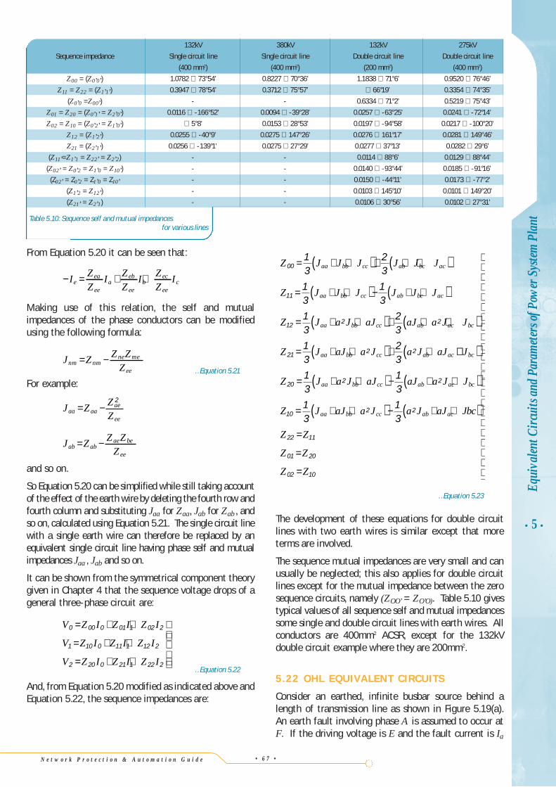
The sequence mutual impedances are very small and canusually be neglected; this also applies for double circuitlines except for the mutual impedance between the zerosequence circuits, namely (ZOO’ = ZO’O). Table 5.10 givestypical values of all sequence self and mutual impedancessome single and double circuit lines with earth wires. Allconductors are 400mm2 ACSR, except for the 132kVdouble circuit example where they are 200mm2.

5.22 OHL EQUIVALENT CIRCUITS

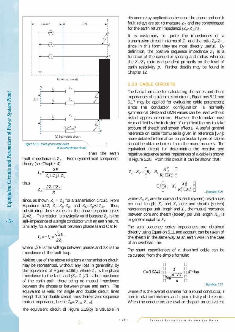
Consider an earthed, infinite busbar source behind alength of transmission line as shown in Figure 5.19(a).An earth fault involving phase A is assumed to occur atF. If the driving voltage is E and the fault current is Ia

Z J J J J J J

Z J J J J J J

Z J a J aJ aJ a J J

Z J aJ a J a J aJ

aa bb cc ab bc ac

aa bb cc ab bc ac

aa bb cc ab ac bc

aa bb cc ab ac

00

11

12 2 2

21 2 2

13

23

13

13

13

23

13

23

= + +( )+ + +( )

= + +( )− + +( )

= + +( )+ + +( )

= + +( )+ + ++( )

= + +( )− + +( )

= + +( )− + +( )=

=

=

J

Z J a J aJ aJ a J J

Z J aJ a J a J aJ Jbc

Z Z

Z Z

Z Z

bc

aa bb cc ab ac bc

aa bb cc ab ac

20 2 2

10 2 2

22 11

01 20

02 10

13

13

13

13

• 5 •Eq

uiva

lent C

ircui

ts an

d Par

amete

rs of

Pow

er S

ystem

Pla

nt

132kV 380kV 132kV 275kV

Sequence impedance Single circuit line Single circuit line Double circuit line Double circuit line

(400 mm2) (400 mm2) (200 mm2) (400 mm2)

Z00 = (Z0’0’) 1.0782 ∠ 73°54’ 0.8227 ∠ 70°36’ 1.1838 ∠ 71°6’ 0.9520 ∠ 76°46’

Z11 = Z22 = (Z1’1’) 0.3947 ∠ 78°54’ 0.3712 ∠ 75°57’ ∠ 66°19’ 0.3354 ∠ 74°35’

(Z0’0 =Z00’) - - 0.6334 ∠ 71°2’ 0.5219 ∠ 75°43’

Z01 = Z20 = (Z0’1’ = Z2’0’) 0.0116 ∠ -166°52’ 0.0094 ∠ -39°28’ 0.0257 ∠ -63°25’ 0.0241 ∠ -72°14’

Z02 = Z10 = (Z0’2’ = Z1’0’) ∠ 5°8’ 0.0153 ∠ 28°53’ 0.0197 ∠ -94°58’ 0.0217 ∠ -100°20’

Z12 = (Z1’2’) 0.0255 ∠ -40°9’ 0.0275 ∠ 147°26’ 0.0276 ∠ 161°17’ 0.0281 ∠ 149°46’

Z21 = (Z2’1’) 0.0256 ∠ -139°1’ 0.0275 ∠ 27°29’ 0.0277 ∠ 37°13’ 0.0282 ∠ 29°6’

(Z11’=Z1’1 = Z22’ = Z2’2) - - 0.0114 ∠ 88°6’ 0.0129 ∠ 88°44’

(Z02’ = Z0’2 = Z1’0 = Z10’) - - 0.0140 ∠ -93°44’ 0.0185 ∠ -91°16’

(Z02’ = Z0’2 = Z1’0 = Z10’ - - 0.0150 ∠ -44°11’ 0.0173 ∠ -77°2’

(Z1’2 = Z12’) - - 0.0103 ∠ 145°10’ 0.0101 ∠ 149°20’

(Z21’ = Z2’1) - - 0.0106 ∠ 30°56’ 0.0102 ∠ 27°31’

Table 5.10: Sequence self and mutual impedancesfor various lines

…Equation 5.23

N e t w o r k P r o t e c t i o n & A u t o m a t i o n G u i d e

then the earthfault impedance is Ze . From symmetrical componenttheory (see Chapter 4):

thus

since, as shown, Z1 = Z2 for a transmission circuit. FromEquations 5.12, Z1=Zp-Zm and ZO=Zp+2Zm. Thus,substituting these values in the above equation givesZe=Zp. This relation is physically valid because Zp is theself-impedance of a single conductor with an earth return.Similarly, for a phase fault between phases B and C at F:

where √_3E is the voltage between phases and 2Z is the

impedance of the fault loop.

Making use of the above relations a transmission circuitmay be represented, without any loss in generality, bythe equivalent of Figure 5.19(b), where Z1 is the phaseimpedance to the fault and (Z0-Z1)/3 is the impedanceof the earth path, there being no mutual impedancebetween the phases or between phase and earth. Theequivalent is valid for single and double circuit linesexcept that for double circuit lines there is zero sequencemutual impedance, hence Z0=(Z00-Z0’0).

The equivalent circuit of Figure 5.19(b) is valuable in

I I EZb c=− = 3

2 1

Z Z Ze = +2

31 0

I EZ Z Za =

+ +3

1 2 0

distance relay applications because the phase and earthfault relays are set to measure Z2 and are compensatedfor the earth return impedance (Z0-Z1)/3.

It is customary to quote the impedances of atransmission circuit in terms of Z1 and the ratio Z0/Z1 ,since in this form they are most directly useful. Bydefinition, the positive sequence impedance Z1 is afunction of the conductor spacing and radius, whereasthe Z0/Z1 ratio is dependent primarily on the level ofearth resistivity ρ. Further details may be found inChapter 12.

5.23 CABLE CIRCUITS

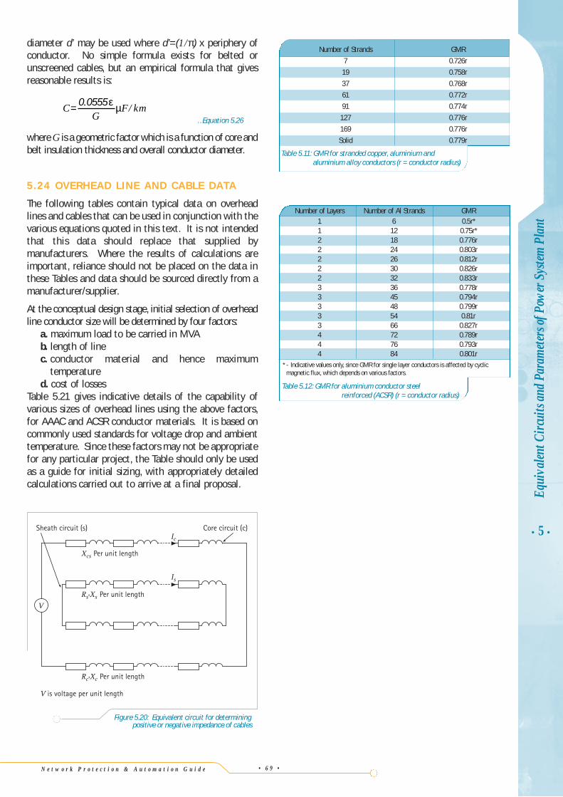
The basic formulae for calculating the series and shuntimpedances of a transmission circuit, Equations 5.11 and5.17 may be applied for evaluating cable parameters;since the conductor configuration is normallysymmetrical GMD and GMR values can be used withoutrisk of appreciable errors. However, the formulae mustbe modified by the inclusion of empirical factors to takeaccount of sheath and screen effects. A useful generalreference on cable formulae is given in reference [5.4];more detailed information on particular types of cablesshould be obtained direct from the manufacturers. Theequivalent circuit for determining the positive andnegative sequence series impedances of a cable is shownin Figure 5.20. From this circuit it can be shown that:

…Equation 5.24

where Rc, Rs are the core and sheath (screen) resistancesper unit length, Xc and Xs core and sheath (screen)reactances per unit length and Xcs the mutual reactancebetween core and sheath (screen) per unit length. Xcs isin general equal to Xs.

The zero sequence series impedances are obtaineddirectly using Equation 5.11 and account can be taken ofthe sheath in the same way as an earth wire in the caseof an overhead line.

The shunt capacitances of a sheathed cable can becalculated from the simple formula:

…Equation 5.25

where d is the overall diameter for a round conductor, Tcore insulation thickness and ε permittivity of dielectric.When the conductors are oval or shaped, an equivalent

Cd T

d

F km=+

0 0241 12

.log

/ε µ

Z Z R R XR X

j X X XR X

c scs

s s

c scs

s s

1 2

2

2 2

2

2 2

= = ++

+ −+

• 5 •

Equi

valen

t Circ

uits

and P

aram

eters

ofPo

wer

Sys

tem P

lant

• 6 8 •

(a) Actual circuit

C

B

A

E

Source LineF

B

C

FS IcIcI Z1

Z1

Z1

(Z0-Z )/3

IbIbI

IaIA

E

(b) Equivalent circuit

3E

~

~

~

Figure 5.19: Three-phase equivalentof a transmission circuit

N e t w o r k P r o t e c t i o n & A u t o m a t i o n G u i d e • 6 9 •

• 5 •Eq

uiva

lent C

ircui

ts an

d Par

amete

rs of

Pow

er S

ystem

Pla

nt

diameter d’ may be used where d’=(1/π) x periphery ofconductor. No simple formula exists for belted orunscreened cables, but an empirical formula that givesreasonable results is:

…Equation 5.26

where G is a geometric factor which is a function of core andbelt insulation thickness and overall conductor diameter.

5.24 OVERHEAD L INE AND CABLE DATA

The following tables contain typical data on overheadlines and cables that can be used in conjunction with thevarious equations quoted in this text. It is not intendedthat this data should replace that supplied bymanufacturers. Where the results of calculations areimportant, reliance should not be placed on the data inthese Tables and data should be sourced directly from amanufacturer/supplier.

At the conceptual design stage, initial selection of overheadline conductor size will be determined by four factors:

a. maximum load to be carried in MVAb. length of linec. conductor material and hence maximum

temperatured. cost of losses

Table 5.21 gives indicative details of the capability ofvarious sizes of overhead lines using the above factors,for AAAC and ACSR conductor materials. It is based oncommonly used standards for voltage drop and ambienttemperature. Since these factors may not be appropriatefor any particular project, the Table should only be usedas a guide for initial sizing, with appropriately detailedcalculations carried out to arrive at a final proposal.

CG

F km= 0 0555. /ε µ

Table 5.12: GMR for aluminium conductor steelreinforced (ACSR) (r = conductor radius)

Number of Layers Number of Al Strands GMR1 6 0.5r*1 12 0.75r*2 18 0.776r2 24 0.803r2 26 0.812r2 30 0.826r2 32 0.833r3 36 0.778r3 45 0.794r3 48 0.799r3 54 0.81r3 66 0.827r4 72 0.789r4 76 0.793r4 84 0.801r

* - Indicative values only, since GMR for single layer conductors is affected by cyclicmagnetic flux, which depends on various factors.

Xcs Per unit length

Ic

Is

Rs'Xs Per unit length

Rc'Xc Per unit length

V

V is voltage per unit length

Sheath circuit (s) Core circuit (c)

Figure 5.20: Equivalent circuit for determiningpositive or negative impedance of cables

Number of Strands GMR

7 0.726r

19 0.758r

37 0.768r

61 0.772r

91 0.774r

127 0.776r

169 0.776r

Solid 0.779r

Table 5.11: GMR for stranded copper, aluminium andaluminium alloy conductors (r = conductor radius)

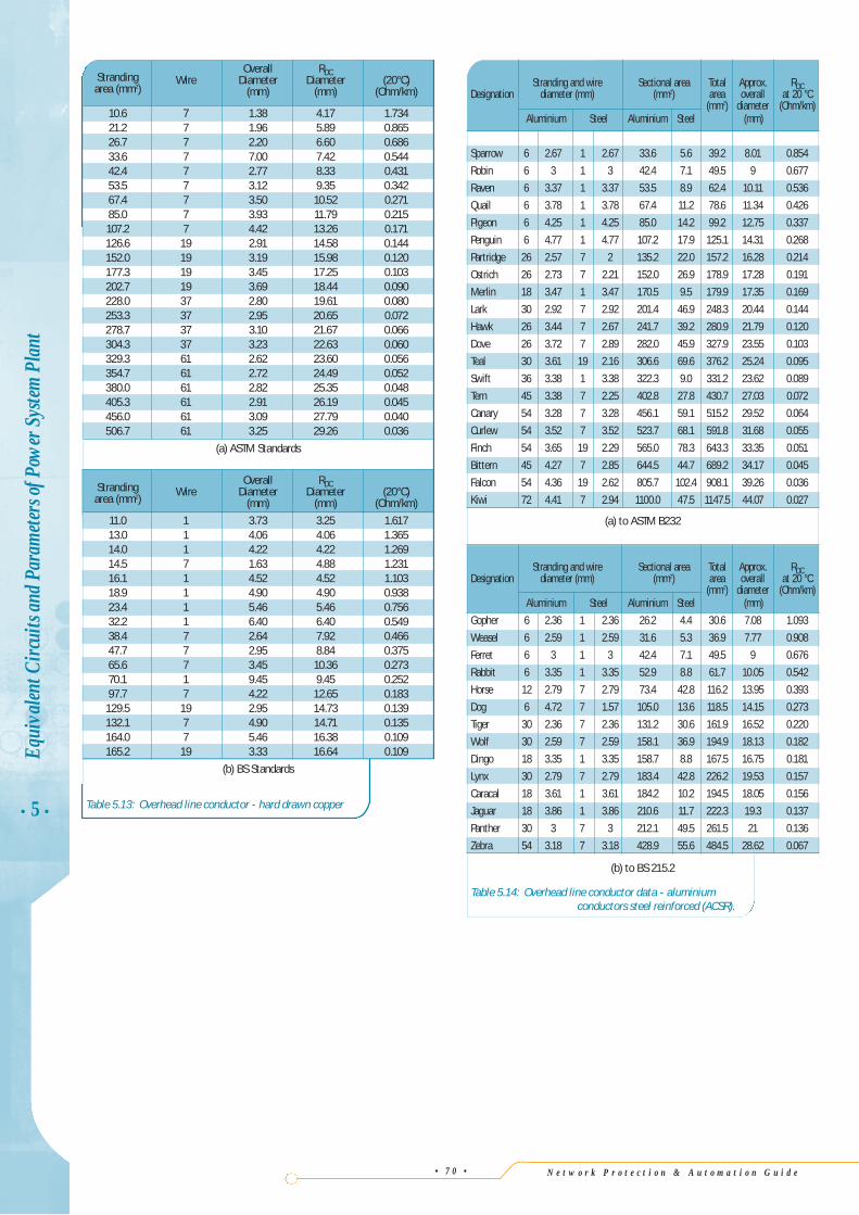
N e t w o r k P r o t e c t i o n & A u t o m a t i o n G u i d e

• 5 •

Equi

valen

t Circ

uits

and P

aram

eters

ofPo

wer

Sys

tem P

lant

• 7 0 •

Stranding and wire Sectional area Total Approx. RDCDesignation diameter (mm) (mm2) area overall at 20 °C

(mm2) diameter (Ohm/km)Aluminium Steel Aluminium Steel (mm)

Gopher 6 2.36 1 2.36 26.2 4.4 30.6 7.08 1.093

Weasel 6 2.59 1 2.59 31.6 5.3 36.9 7.77 0.908

Ferret 6 3 1 3 42.4 7.1 49.5 9 0.676

Rabbit 6 3.35 1 3.35 52.9 8.8 61.7 10.05 0.542

Horse 12 2.79 7 2.79 73.4 42.8 116.2 13.95 0.393

Dog 6 4.72 7 1.57 105.0 13.6 118.5 14.15 0.273

Tiger 30 2.36 7 2.36 131.2 30.6 161.9 16.52 0.220

Wolf 30 2.59 7 2.59 158.1 36.9 194.9 18.13 0.182

Dingo 18 3.35 1 3.35 158.7 8.8 167.5 16.75 0.181

Lynx 30 2.79 7 2.79 183.4 42.8 226.2 19.53 0.157

Caracal 18 3.61 1 3.61 184.2 10.2 194.5 18.05 0.156

Jaguar 18 3.86 1 3.86 210.6 11.7 222.3 19.3 0.137

Panther 30 3 7 3 212.1 49.5 261.5 21 0.136

Zebra 54 3.18 7 3.18 428.9 55.6 484.5 28.62 0.067

Stranding and wire Sectional area Total Approx. RDCDesignation diameter (mm) (mm2) area overall at 20 °C

(mm2) diameter (Ohm/km)Aluminium Steel Aluminium Steel (mm)

Sparrow 6 2.67 1 2.67 33.6 5.6 39.2 8.01 0.854

Robin 6 3 1 3 42.4 7.1 49.5 9 0.677

Raven 6 3.37 1 3.37 53.5 8.9 62.4 10.11 0.536

Quail 6 3.78 1 3.78 67.4 11.2 78.6 11.34 0.426

Pigeon 6 4.25 1 4.25 85.0 14.2 99.2 12.75 0.337

Penguin 6 4.77 1 4.77 107.2 17.9 125.1 14.31 0.268

Partridge 26 2.57 7 2 135.2 22.0 157.2 16.28 0.214

Ostrich 26 2.73 7 2.21 152.0 26.9 178.9 17.28 0.191

Merlin 18 3.47 1 3.47 170.5 9.5 179.9 17.35 0.169

Lark 30 2.92 7 2.92 201.4 46.9 248.3 20.44 0.144

Hawk 26 3.44 7 2.67 241.7 39.2 280.9 21.79 0.120

Dove 26 3.72 7 2.89 282.0 45.9 327.9 23.55 0.103

Teal 30 3.61 19 2.16 306.6 69.6 376.2 25.24 0.095

Swift 36 3.38 1 3.38 322.3 9.0 331.2 23.62 0.089

Tern 45 3.38 7 2.25 402.8 27.8 430.7 27.03 0.072

Canary 54 3.28 7 3.28 456.1 59.1 515.2 29.52 0.064

Curlew 54 3.52 7 3.52 523.7 68.1 591.8 31.68 0.055

Finch 54 3.65 19 2.29 565.0 78.3 643.3 33.35 0.051

Bittern 45 4.27 7 2.85 644.5 44.7 689.2 34.17 0.045

Falcon 54 4.36 19 2.62 805.7 102.4 908.1 39.26 0.036

Kiwi 72 4.41 7 2.94 1100.0 47.5 1147.5 44.07 0.027

(a) to ASTM B232

(b) to BS 215.2

Table 5.14: Overhead line conductor data - aluminiumconductors steel reinforced (ACSR).

Overall RDCStranding Wire Diameter Diameter (20°C) area (mm2) (mm) (mm) (Ohm/km)

10.6 7 1.38 4.17 1.73421.2 7 1.96 5.89 0.86526.7 7 2.20 6.60 0.68633.6 7 7.00 7.42 0.54442.4 7 2.77 8.33 0.43153.5 7 3.12 9.35 0.34267.4 7 3.50 10.52 0.27185.0 7 3.93 11.79 0.215107.2 7 4.42 13.26 0.171126.6 19 2.91 14.58 0.144152.0 19 3.19 15.98 0.120177.3 19 3.45 17.25 0.103202.7 19 3.69 18.44 0.090228.0 37 2.80 19.61 0.080253.3 37 2.95 20.65 0.072278.7 37 3.10 21.67 0.066304.3 37 3.23 22.63 0.060329.3 61 2.62 23.60 0.056354.7 61 2.72 24.49 0.052380.0 61 2.82 25.35 0.048405.3 61 2.91 26.19 0.045456.0 61 3.09 27.79 0.040506.7 61 3.25 29.26 0.036

(a) ASTM Standards

Overall RDCStranding Wire Diameter Diameter (20°C) area (mm2) (mm) (mm) (Ohm/km)

11.0 1 3.73 3.25 1.61713.0 1 4.06 4.06 1.36514.0 1 4.22 4.22 1.26914.5 7 1.63 4.88 1.23116.1 1 4.52 4.52 1.10318.9 1 4.90 4.90 0.93823.4 1 5.46 5.46 0.75632.2 1 6.40 6.40 0.54938.4 7 2.64 7.92 0.46647.7 7 2.95 8.84 0.37565.6 7 3.45 10.36 0.27370.1 1 9.45 9.45 0.25297.7 7 4.22 12.65 0.183129.5 19 2.95 14.73 0.139132.1 7 4.90 14.71 0.135164.0 7 5.46 16.38 0.109165.2 19 3.33 16.64 0.109

(b) BS Standards

Table 5.13: Overhead line conductor - hard drawn copper

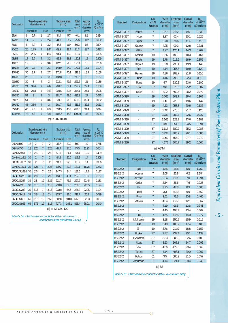
(d) to NF C34-120

Table 5.14: Overhead line conductor data - aluminiumconductors steel reinforced (ACSR).

N e t w o r k P r o t e c t i o n & A u t o m a t i o n G u i d e • 7 1 •

• 5 •Eq

uiva

lent C

ircui

ts an

d Par

amete

rs of

Pow

er S

ystem

Pla

nt

Stranding and wire Sectional area Total Approx. RDCDesignation diameter (mm) (mm2) area overall at 20 °C

(mm2) diameter (Ohm/km)Aluminium Steel Aluminium Steel (mm)

35/6 6 2.7 1 2.7 34.4 5.7 40.1 8.1 0.834

44/32 14 2 7 2.4 44.0 31.7 75.6 11.2 0.652

50/8 6 3.2 1 3.2 48.3 8.0 56.3 9.6 0.594

70/12 26 1.85 7 1.44 69.9 11.4 81.3 11.7 0.413

95/15 26 2.15 7 1.67 94.4 15.3 109.7 13.6 0.305

95/55 12 3.2 7 3.2 96.5 56.3 152.8 16 0.299

120/70 12 3.6 7 3.6 122.1 71.3 193.4 18 0.236

150/25 26 2.7 7 2.1 148.9 24.2 173.1 17.1 0.194

170/40 30 2.7 7 2.7 171.8 40.1 211.8 18.9 0.168

185/30 26 3 7 2.33 183.8 29.8 213.6 19 0.157

210/50 30 3 7 3 212.1 49.5 261.5 21 0.136

265/35 24 3.74 7 2.49 263.7 34.1 297.7 22.4 0.109

305/40 54 2.68 7 2.68 304.6 39.5 344.1 24.1 0.095

380/50 54 3 7 3 381.7 49.5 431.2 27 0.076

550/70 54 3.6 7 3.6 549.7 71.3 620.9 32.4 0.052

560/50 48 3.86 7 3 561.7 49.5 611.2 32.2 0.051

650/45 45 4.3 7 2.87 653.5 45.3 698.8 34.4 0.044

1045/45 72 4.3 7 2.87 1045.6 45.3 1090.9 43 0.028

Stranding and wire Sectional area Total Approxi. RDCDesignation diameter (mm) (mm2) area overall at 20 °C

(mm2) diameter (Ohm/km)Aluminium Steel Aluminium Steel (mm)

CANNA 59.7 12 2 7 2 37.7 22.0 59.7 10 0.765

CANNA 75.5 12 2.25 7 2.25 47.7 27.8 75.5 11.25 0.604

CANNA 93.3 12 2.5 7 2.5 58.9 34.4 93.3 12.5 0.489

CANNA 116.2 30 2 7 2 94.2 22.0 116.2 14 0.306

CROCUS 116.2 30 2 7 2 94.2 22.0 116.2 14 0.306

CANNA 147.1 30 2.25 7 2.25 119.3 27.8 147.1 15.75 0.243

CROCUS 181.6 30 2.5 7 2.5 147.3 34.4 181.6 17.5 0.197

CROCUS 228 30 2.8 7 2.8 184.7 43.1 227.8 19.6 0.157

CROCUS 297 36 2.8 19 2.25 221.7 75.5 297.2 22.45 0.131

CANNA 288 30 3.15 7 3.15 233.8 54.6 288.3 22.05 0.124

CROCUS 288 30 3.15 7 3.15 233.8 54.6 288.3 22.05 0.124

CROCUS 412 32 3.6 19 2.4 325.7 86.0 411.7 26.4 0.089

CROCUS 612 66 3.13 19 2.65 507.8 104.8 612.6 32.03 0.057

CROCUS 865 66 3.72 19 3.15 717.3 148.1 865.4 38.01 0.040

(c) to DIN 48204

No. Wire Sectional Overall RDCStandard Designation of Al diameter area diameter at 20°C

Strands (mm) (mm2) (mm) (Ohm/km)

BS 3242 Box 7 1.85 18.8 5.6 1.750

BS 3242 Acacia 7 2.08 23.8 6.2 1.384

BS 3242 Almond 7 2.34 30.1 7.0 1.094

BS 3242 Cedar 7 2.54 35.5 7.6 0.928

BS 3242 Fir 7 2.95 47.8 8.9 0.688

BS 3242 Hazel 7 3.3 59.9 9.9 0.550

BS 3242 Pine 7 3.61 71.6 10.8 0.460

BS 3242 Willow 7 4.04 89.7 12.1 0.367

BS 3242 - 7 4.19 96.5 12.6 0.341

BS 3242 - 7 4.45 108.9 13.4 0.302

BS 3242 Oak 7 4.65 118.9 14.0 0.277

BS 3242 Mullberry 19 3.18 150.9 15.9 0.219

BS 3242 Ash 19 3.48 180.7 17.4 0.183

BS 3242 Elm 19 3.76 211.0 18.8 0.157

BS 3242 Poplar 37 2.87 239.4 20.1 0.139

BS 3242 Sycamore 37 3.23 303.2 22.6 0.109

BS 3242 Upas 37 3.53 362.1 24.7 0.092

BS 3242 Yew 37 4.06 479.0 28.4 0.069

BS 3242 Totara 37 4.14 498.1 29.0 0.067

BS 3242 Rubus 61 3.5 586.9 31.5 0.057

BS 3242 Araucaria 61 4.14 821.1 28.4 0.040

No. Wire Sectional Overall RDCStandard Designation of Al diameter area diameter at 20°C

Strands (mm) (mm2) (mm) (Ohm/km)

ASTM B-397 Kench 7 2.67 39.2 8.0 0.838

ASTM B-397 Kibe 7 3.37 62.4 10.1 0.526

ASTM B-397 Kayak 7 3.78 78.6 11.4 0.418

ASTM B-397 Kopeck 7 4.25 99.3 12.8 0.331

ASTM B-397 Kittle 7 4.77 125.1 14.3 0.262

ASTM B-397 Radian 19 3.66 199.9 18.3 0.164

ASTM B-397 Rede 19 3.78 212.6 18.9 0.155

ASTM B-397 Ragout 19 3.98 236.4 19.9 0.140

ASTM B-397 Rex 19 4.14 255.8 19.9 0.129

ASTM B-397 Remex 19 4.36 283.7 21.8 0.116

ASTM B-397 Ruble 19 4.46 296.8 22.4 0.111

ASTM B-397 Rune 19 4.7 330.6 23.6 0.100

ASTM B-397 Spar 37 3.6 376.6 25.2 0.087

ASTM B-397 Solar 37 4.02 469.6 28.2 0.070

ASTM B-399 - 19 3.686 202.7 18.4 0.165

ASTM B-399 - 19 3.909 228.0 19.6 0.147

ASTM B-399 - 19 4.12 253.3 20.6 0.132

ASTM B-399 - 37 3.096 278.5 21.7 0.120

ASTM B-399 - 37 3.233 303.7 22.6 0.110

ASTM B-399 - 37 3.366 329.2 23.6 0.102

ASTM B-399 - 37 3.493 354.6 24.5 0.094

ASTM B-399 - 37 3.617 380.2 25.3 0.088

ASTM B-399 - 37 3.734 405.2 26.1 0.083

ASTM B-399 - 37 3.962 456.2 27.7 0.073

ASTM B-399 - 37 4.176 506.8 29.2 0.066

(a) ASTM

(b) BS

Table 5.15: Overhead line conductor data - aluminium alloy.

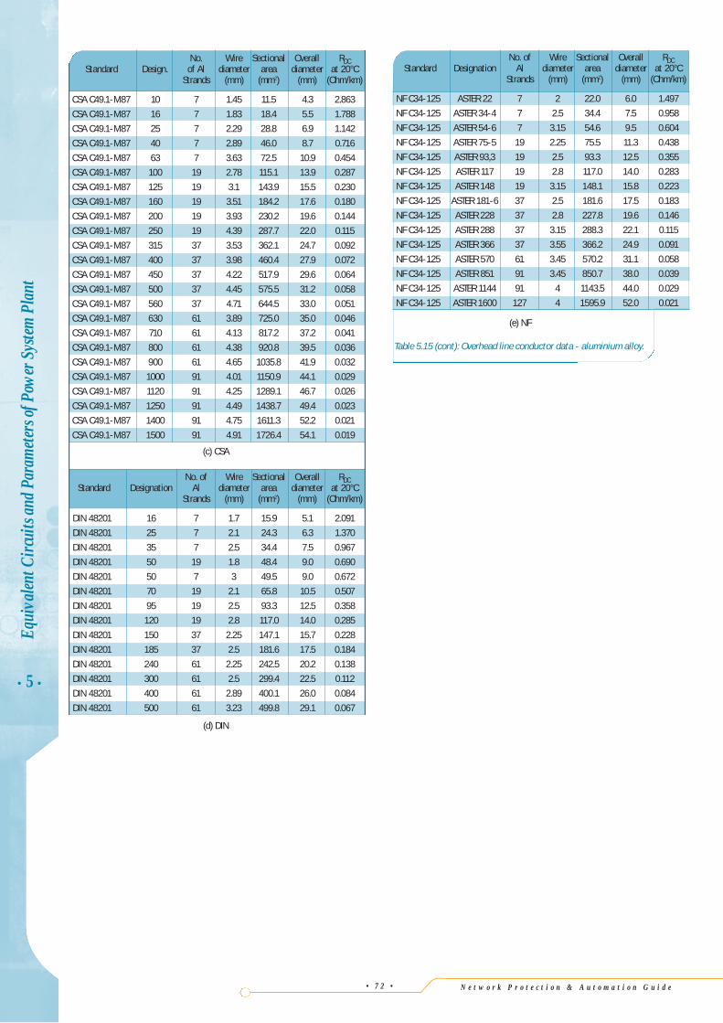
N e t w o r k P r o t e c t i o n & A u t o m a t i o n G u i d e

• 5 •

Equi

valen

t Circ

uits

and P

aram

eters

ofPo

wer

Sys

tem P

lant

• 7 2 •

No. of Wire Sectional Overall RDCStandard Designation Al diameter area diameter at 20°C

Strands (mm) (mm2) (mm) (Ohm/km)

NF C34-125 ASTER 22 7 2 22.0 6.0 1.497

NF C34-125 ASTER 34-4 7 2.5 34.4 7.5 0.958

NF C34-125 ASTER 54-6 7 3.15 54.6 9.5 0.604

NF C34-125 ASTER 75-5 19 2.25 75.5 11.3 0.438

NF C34-125 ASTER 93,3 19 2.5 93.3 12.5 0.355

NF C34-125 ASTER 117 19 2.8 117.0 14.0 0.283

NF C34-125 ASTER 148 19 3.15 148.1 15.8 0.223

NF C34-125 ASTER 181-6 37 2.5 181.6 17.5 0.183

NF C34-125 ASTER 228 37 2.8 227.8 19.6 0.146

NF C34-125 ASTER 288 37 3.15 288.3 22.1 0.115

NF C34-125 ASTER 366 37 3.55 366.2 24.9 0.091

NF C34-125 ASTER 570 61 3.45 570.2 31.1 0.058

NF C34-125 ASTER 851 91 3.45 850.7 38.0 0.039

NF C34-125 ASTER 1144 91 4 1143.5 44.0 0.029

NF C34-125 ASTER 1600 127 4 1595.9 52.0 0.021

No. of Wire Sectional Overall RDCStandard Designation Al diameter area diameter at 20°C

Strands (mm) (mm2) (mm) (Ohm/km)

DIN 48201 16 7 1.7 15.9 5.1 2.091

DIN 48201 25 7 2.1 24.3 6.3 1.370

DIN 48201 35 7 2.5 34.4 7.5 0.967

DIN 48201 50 19 1.8 48.4 9.0 0.690

DIN 48201 50 7 3 49.5 9.0 0.672

DIN 48201 70 19 2.1 65.8 10.5 0.507

DIN 48201 95 19 2.5 93.3 12.5 0.358

DIN 48201 120 19 2.8 117.0 14.0 0.285

DIN 48201 150 37 2.25 147.1 15.7 0.228

DIN 48201 185 37 2.5 181.6 17.5 0.184

DIN 48201 240 61 2.25 242.5 20.2 0.138

DIN 48201 300 61 2.5 299.4 22.5 0.112

DIN 48201 400 61 2.89 400.1 26.0 0.084

DIN 48201 500 61 3.23 499.8 29.1 0.067

No. Wire Sectional Overall RDCStandard Design. of Al diameter area diameter at 20°C

Strands (mm) (mm2) (mm) (Ohm/km)

CSA C49.1-M87 10 7 1.45 11.5 4.3 2.863

CSA C49.1-M87 16 7 1.83 18.4 5.5 1.788

CSA C49.1-M87 25 7 2.29 28.8 6.9 1.142

CSA C49.1-M87 40 7 2.89 46.0 8.7 0.716

CSA C49.1-M87 63 7 3.63 72.5 10.9 0.454

CSA C49.1-M87 100 19 2.78 115.1 13.9 0.287

CSA C49.1-M87 125 19 3.1 143.9 15.5 0.230

CSA C49.1-M87 160 19 3.51 184.2 17.6 0.180

CSA C49.1-M87 200 19 3.93 230.2 19.6 0.144

CSA C49.1-M87 250 19 4.39 287.7 22.0 0.115

CSA C49.1-M87 315 37 3.53 362.1 24.7 0.092

CSA C49.1-M87 400 37 3.98 460.4 27.9 0.072

CSA C49.1-M87 450 37 4.22 517.9 29.6 0.064

CSA C49.1-M87 500 37 4.45 575.5 31.2 0.058

CSA C49.1-M87 560 37 4.71 644.5 33.0 0.051

CSA C49.1-M87 630 61 3.89 725.0 35.0 0.046

CSA C49.1-M87 710 61 4.13 817.2 37.2 0.041

CSA C49.1-M87 800 61 4.38 920.8 39.5 0.036

CSA C49.1-M87 900 61 4.65 1035.8 41.9 0.032

CSA C49.1-M87 1000 91 4.01 1150.9 44.1 0.029

CSA C49.1-M87 1120 91 4.25 1289.1 46.7 0.026

CSA C49.1-M87 1250 91 4.49 1438.7 49.4 0.023

CSA C49.1-M87 1400 91 4.75 1611.3 52.2 0.021

CSA C49.1-M87 1500 91 4.91 1726.4 54.1 0.019

(c) CSA

(d) DIN

(e) NF

Table 5.15 (cont): Overhead line conductor data - aluminium alloy.

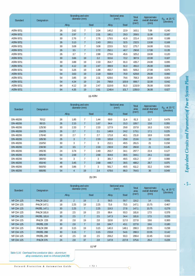
N e t w o r k P r o t e c t i o n & A u t o m a t i o n G u i d e • 7 3 •

• 5 •Eq

uiva

lent C

ircui

ts an

d Par

amete

rs of

Pow

er S

ystem

Pla

ntStranding and wire Sectional area

Standard Designationdiameter (mm) (mm2)

Alloy Steel Alloy Steel

NF C34-125 PHLOX 116.2 18 2 19 2 56.5 59.7 116.2 14 0.591

NF C34-125 PHLOX 147.1 18 2.25 19 2.25 71.6 75.5 147.1 15.75 0.467

NF C34-125 PASTEL 147.1 30 2.25 7 2.25 119.3 27.8 147.1 15.75 0.279

NF C34-125 PHLOX 181.6 18 2.5 19 2.5 88.4 93.3 181.6 17.5 0.378

NF C34-125 PASTEL 181.6 30 2.5 7 2.5 147.3 34.4 181.6 17.5 0.226

NF C34-125 PHLOX 228 18 2.8 19 2.8 110.8 117.0 227.8 19.6 0.300

NF C34-125 PASTEL 228 30 2.8 7 2.8 184.7 43.1 227.8 19.6 0.180

NF C34-125 PHLOX 288 18 3.15 19 3.15 140.3 148.1 288.3 22.05 0.238

NF C34-125 PASTEL 288 30 3.15 7 3.15 233.8 54.6 288.3 22.05 0.142

NF C34-125 PASTEL 299 42 2.5 19 2.5 206.2 93.3 299.4 22.45 0.162

NF C34-125 PHLOX 376 24 2.8 37 2.8 147.8 227.8 375.6 26.4 0.226

Stranding and wire Sectional area

Standard Designationdiameter (mm) (mm2)

Alloy Steel Alloy Steel

DIN 48206 70/12 26 1.85 7 1.44 69.9 11.4 81.3 11.7 0.479

DIN 48206 95/15 26 2.15 7 1.67 94.4 15.3 109.7 13.6 0.355

DIN 48206 125/30 30 2.33 7 2.33 127.9 29.8 157.8 16.3 0.262

DIN 48206 150/25 26 2.7 7 2.1 148.9 24.2 173.1 17.1 0.225

DIN 48206 170/40 30 2.7 7 2.7 171.8 40.1 211.8 18.9 0.195

DIN 48206 185/30 26 3 7 2.33 183.8 29.8 213.6 19 0.182

DIN 48206 210/50 30 3 7 3 212.1 49.5 261.5 21 0.158

DIN 48206 230/30 24 3.5 7 2.33 230.9 29.8 260.8 21 0.145

DIN 48206 265/35 24 3.74 7 2.49 263.7 34.1 297.7 22.4 0.127

DIN 48206 305/40 54 2.68 7 2.68 304.6 39.5 344.1 24.1 0.110

DIN 48206 380/50 54 3 7 3 381.7 49.5 431.2 27 0.088

DIN 48206 450/40 48 3.45 7 2.68 448.7 39.5 488.2 28.7 0.075

DIN 48206 560/50 48 3.86 7 3 561.7 49.5 611.2 32.2 0.060

DIN 48206 680/85 54 4 19 2.4 678.6 86.0 764.5 36 0.049

(b) DIN

(c) NF

Table 5.16: Overhead line conductor data – aluminiumalloy conductors, steel re-inforced (AACSR)

Stranding and wire Sectional area

Standard Designationdiameter (mm) (mm2)

Alloy Steel Alloy Steel

ASTM B711 26 2.62 7 2.04 140.2 22.9 163.1 7.08 0.240

ASTM B711 26 2.97 7 2.31 180.1 29.3 209.5 11.08 0.187

ASTM B711 30 2.76 7 2.76 179.5 41.9 221.4 12.08 0.188

ASTM B711 26 3.13 7 2.43 200.1 32.5 232.5 13.08 0.168

ASTM B711 30 3.08 7 3.08 223.5 52.2 275.7 16.08 0.151

ASTM B711 26 3.5 7 2.72 250.1 40.7 290.8 17.08 0.135

ASTM B711 26 3.7 7 2.88 279.6 45.6 325.2 19.08 0.120

ASTM B711 30 3.66 19 2.2 315.6 72.2 387.9 22.08 0.107

ASTM B711 30 3.88 19 2.33 354.7 81.0 435.7 24.08 0.095

ASTM B711 30 4.12 19 2.47 399.9 91.0 491.0 26.08 0.084

ASTM B711 54 3.26 19 1.98 450.7 58.5 509.2 27.08 0.075

ASTM B711 54 3.63 19 2.18 558.9 70.9 629.8 29.08 0.060

ASTM B711 54 3.85 19 2.31 628.6 79.6 708.3 30.08 0.054

ASTM B711 54 4.34 19 2.6 798.8 100.9 899.7 32.08 0.042

ASTM B711 84 4.12 19 2.47 1119.9 91.0 1210.9 35.08 0.030

ASTM B711 84 4.35 19 2.61 1248.4 101.7 1350.0 36.08 0.027

(a) ASTM

Totalarea

(mm2)

Approximateoverall diameter

(mm)

RDC at 20 °C(ohm/km)

Totalarea

(mm2)

Approximateoverall diameter

(mm)

RDC at 20 °C(ohm/km)

Totalarea

(mm2)

Approximateoverall diameter

(mm)

RDC at 20 °C(ohm/km)

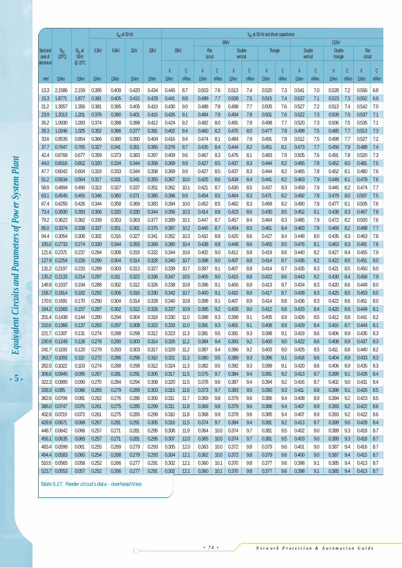
N e t w o r k P r o t e c t i o n & A u t o m a t i o n G u i d e

• 5 •

Equi

valen

t Circ

uits

and P

aram

eters

ofPo

wer

Sys

tem P

lant

• 7 4 •

XAC at 50 Hz XAC at 50 Hz and shunt capacitance

66kV 132kV

Sectional RDC RAC at 3.3kV 6.6kV 11kV 22kV 33kV Flat Double Triangle Double Double Flatarea of (20°C) 50Hz circuit vertical vertical triangle circuit

aluminium @ 20°C

X C X C X C X C X C X C X C

mm2 Ω/km Ω/km Ω/km Ω/km Ω/km Ω/km Ω/km nF/km Ω/km nF/km Ω/km nF/km Ω/km nF/km Ω/km nF/km Ω/km nF/km Ω/km nF/km

13.3 2.1586 2.159 0.395 0.409 0.420 0.434 0.445 8.7 0.503 7.6 0.513 7.4 0.520 7.3 0.541 7.0 0.528 7.2 0.556 6.8

15.3 1.8771 1.877 0.391 0.405 0.415 0.429 0.441 8.8 0.499 7.7 0.508 7.5 0.515 7.4 0.537 7.1 0.523 7.3 0.552 6.9

21.2 1.3557 1.356 0.381 0.395 0.405 0.419 0.430 9.0 0.488 7.8 0.498 7.7 0.505 7.6 0.527 7.2 0.513 7.4 0.542 7.0

23.9 1.2013 1.201 0.376 0.390 0.401 0.415 0.426 9.1 0.484 7.9 0.494 7.8 0.501 7.6 0.522 7.3 0.509 7.5 0.537 7.1

26.2 1.0930 1.093 0.374 0.388 0.398 0.412 0.424 9.2 0.482 8.0 0.491 7.8 0.498 7.7 0.520 7.3 0.506 7.5 0.535 7.1

28.3 1.0246 1.025 0.352 0.366 0.377 0.391 0.402 9.4 0.460 8.2 0.470 8.0 0.477 7.8 0.498 7.5 0.485 7.7 0.513 7.3

33.6 0.8535 0.854 0.366 0.380 0.390 0.404 0.416 9.4 0.474 8.1 0.484 7.9 0.491 7.8 0.512 7.5 0.499 7.7 0.527 7.2

37.7 0.7647 0.765 0.327 0.341 0.351 0.365 0.376 9.7 0.435 8.4 0.444 8.2 0.451 8.1 0.473 7.7 0.459 7.9 0.488 7.4

42.4 0.6768 0.677 0.359 0.373 0.383 0.397 0.409 9.6 0.467 8.3 0.476 8.1 0.483 7.9 0.505 7.6 0.491 7.8 0.520 7.3

44.0 0.6516 0.652 0.320 0.334 0.344 0.358 0.369 9.9 0.427 8.5 0.437 8.3 0.444 8.2 0.465 7.8 0.452 8.0 0.481 7.5

47.7 0.6042 0.604 0.319 0.333 0.344 0.358 0.369 9.9 0.427 8.5 0.437 8.3 0.444 8.2 0.465 7.8 0.452 8.1 0.480 7.6

51.2 0.5634 0.564 0.317 0.331 0.341 0.355 0.367 10.0 0.425 8.6 0.434 8.4 0.441 8.2 0.463 7.9 0.449 8.1 0.478 7.6

58.9 0.4894 0.490 0.313 0.327 0.337 0.351 0.362 10.1 0.421 8.7 0.430 8.5 0.437 8.3 0.459 7.9 0.445 8.2 0.474 7.7

63.1 0.4545 0.455 0.346 0.360 0.371 0.385 0.396 9.9 0.454 8.5 0.464 8.3 0.471 8.2 0.492 7.8 0.479 8.0 0.507 7.5

67.4 0.4255 0.426 0.344 0.358 0.369 0.383 0.394 10.0 0.452 8.5 0.462 8.3 0.469 8.2 0.490 7.8 0.477 8.1 0.505 7.6

73.4 0.3930 0.393 0.306 0.320 0.330 0.344 0.356 10.3 0.414 8.8 0.423 8.6 0.430 8.5 0.452 8.1 0.438 8.3 0.467 7.8

79.2 0.3622 0.362 0.339 0.353 0.363 0.377 0.389 10.1 0.447 8.7 0.457 8.4 0.464 8.3 0.485 7.9 0.472 8.2 0.500 7.6

85.0 0.3374 0.338 0.337 0.351 0.361 0.375 0.387 10.2 0.445 8.7 0.454 8.5 0.461 8.4 0.483 7.9 0.469 8.2 0.498 7.7

94.4 0.3054 0.306 0.302 0.316 0.327 0.341 0.352 10.3 0.410 8.8 0.420 8.6 0.427 8.4 0.448 8.0 0.435 8.3 0.463 7.8

105.0 0.2733 0.274 0.330 0.344 0.355 0.369 0.380 10.4 0.438 8.8 0.448 8.6 0.455 8.5 0.476 8.1 0.463 8.3 0.491 7.8

121.6 0.2371 0.237 0.294 0.308 0.318 0.332 0.344 10.6 0.402 9.0 0.412 8.8 0.419 8.6 0.440 8.2 0.427 8.4 0.455 7.9

127.9 0.2254 0.226 0.290 0.304 0.314 0.328 0.340 10.7 0.398 9.0 0.407 8.8 0.414 8.7 0.436 8.2 0.422 8.5 0.451 8.0

131.2 0.2197 0.220 0.289 0.303 0.313 0.327 0.339 10.7 0.397 9.1 0.407 8.8 0.414 8.7 0.435 8.3 0.421 8.5 0.450 8.0

135.2 0.2133 0.214 0.297 0.311 0.322 0.336 0.347 10.5 0.405 9.0 0.415 8.8 0.422 8.6 0.443 8.2 0.430 8.4 0.458 7.9

148.9 0.1937 0.194 0.288 0.302 0.312 0.326 0.338 10.8 0.396 9.1 0.406 8.9 0.413 8.7 0.434 8.3 0.420 8.6 0.449 8.0

158.7 0.1814 0.182 0.292 0.306 0.316 0.330 0.342 10.7 0.400 9.1 0.410 8.9 0.417 8.7 0.438 8.3 0.425 8.5 0.453 8.0

170.5 0.1691 0.170 0.290 0.304 0.314 0.328 0.340 10.8 0.398 9.1 0.407 8.9 0.414 8.8 0.436 8.3 0.422 8.6 0.451 8.0

184.2 0.1565 0.157 0.287 0.302 0.312 0.326 0.337 10.9 0.395 9.2 0.405 9.0 0.412 8.8 0.433 8.4 0.420 8.6 0.449 8.1

201.4 0.1438 0.144 0.280 0.294 0.304 0.318 0.330 11.0 0.388 9.3 0.398 9.1 0.405 8.9 0.426 8.5 0.412 8.8 0.441 8.2

210.6 0.1366 0.137 0.283 0.297 0.308 0.322 0.333 11.0 0.391 9.3 0.401 9.1 0.408 8.9 0.429 8.4 0.416 8.7 0.444 8.1

221.7 0.1307 0.131 0.274 0.288 0.298 0.312 0.323 11.3 0.381 9.5 0.391 9.3 0.398 9.1 0.419 8.6 0.406 8.9 0.435 8.3

230.9 0.1249 0.126 0.276 0.290 0.300 0.314 0.326 11.2 0.384 9.4 0.393 9.2 0.400 9.0 0.422 8.6 0.408 8.9 0.437 8.3

241.7 0.1193 0.120 0.279 0.293 0.303 0.317 0.329 11.2 0.387 9.4 0.396 9.2 0.403 9.0 0.425 8.5 0.411 8.8 0.440 8.2

263.7 0.1093 0.110 0.272 0.286 0.296 0.310 0.321 11.3 0.380 9.5 0.389 9.3 0.396 9.1 0.418 8.6 0.404 8.9 0.433 8.3

282.0 0.1022 0.103 0.274 0.288 0.298 0.312 0.324 11.3 0.382 9.5 0.392 9.3 0.399 9.1 0.420 8.6 0.406 8.9 0.435 8.3

306.6 0.0945 0.095 0.267 0.281 0.291 0.305 0.317 11.5 0.375 9.7 0.384 9.4 0.391 9.2 0.413 8.7 0.399 9.1 0.428 8.4

322.3 0.0895 0.090 0.270 0.284 0.294 0.308 0.320 11.5 0.378 9.6 0.387 9.4 0.394 9.2 0.416 8.7 0.402 9.0 0.431 8.4

339.3 0.085 0.086 0.265 0.279 0.289 0.303 0.315 11.6 0.373 9.7 0.383 9.5 0.390 9.3 0.411 8.8 0.398 9.1 0.426 8.5

362.6 0.0799 0.081 0.262 0.276 0.286 0.300 0.311 11.7 0.369 9.8 0.379 9.6 0.386 9.4 0.408 8.9 0.394 9.2 0.423 8.5

386.0 0.0747 0.076 0.261 0.275 0.285 0.299 0.311 11.8 0.369 9.8 0.379 9.6 0.386 9.4 0.407 8.9 0.393 9.2 0.422 8.6

402.8 0.0719 0.073 0.261 0.275 0.285 0.299 0.310 11.8 0.368 9.9 0.378 9.6 0.385 9.4 0.407 8.9 0.393 9.2 0.422 8.6

428.9 0.0671 0.068 0.267 0.281 0.291 0.305 0.316 11.5 0.374 9.7 0.384 9.4 0.391 9.2 0.413 8.7 0.399 9.0 0.428 8.4

448.7 0.0642 0.066 0.257 0.271 0.281 0.295 0.306 11.9 0.364 10.0 0.374 9.7 0.381 9.5 0.402 9.0 0.389 9.3 0.418 8.7

456.1 0.0635 0.065 0.257 0.271 0.281 0.295 0.307 12.0 0.365 10.0 0.374 9.7 0.381 9.5 0.403 9.0 0.389 9.3 0.418 8.7

483.4 0.0599 0.061 0.255 0.269 0.279 0.293 0.305 12.0 0.363 10.0 0.372 9.8 0.379 9.6 0.401 9.0 0.387 9.4 0.416 8.7

494.4 0.0583 0.060 0.254 0.268 0.279 0.293 0.304 12.1 0.362 10.0 0.372 9.8 0.379 9.6 0.400 9.0 0.387 9.4 0.415 8.7

510.5 0.0565 0.058 0.252 0.266 0.277 0.291 0.302 12.1 0.360 10.1 0.370 9.8 0.377 9.6 0.398 9.1 0.385 9.4 0.413 8.7

523.7 0.0553 0.057 0.252 0.266 0.277 0.291 0.302 12.1 0.360 10.1 0.370 9.8 0.377 9.6 0.398 9.1 0.385 9.4 0.413 8.7

Table 5.17: Feeder circuits data - overhead lines

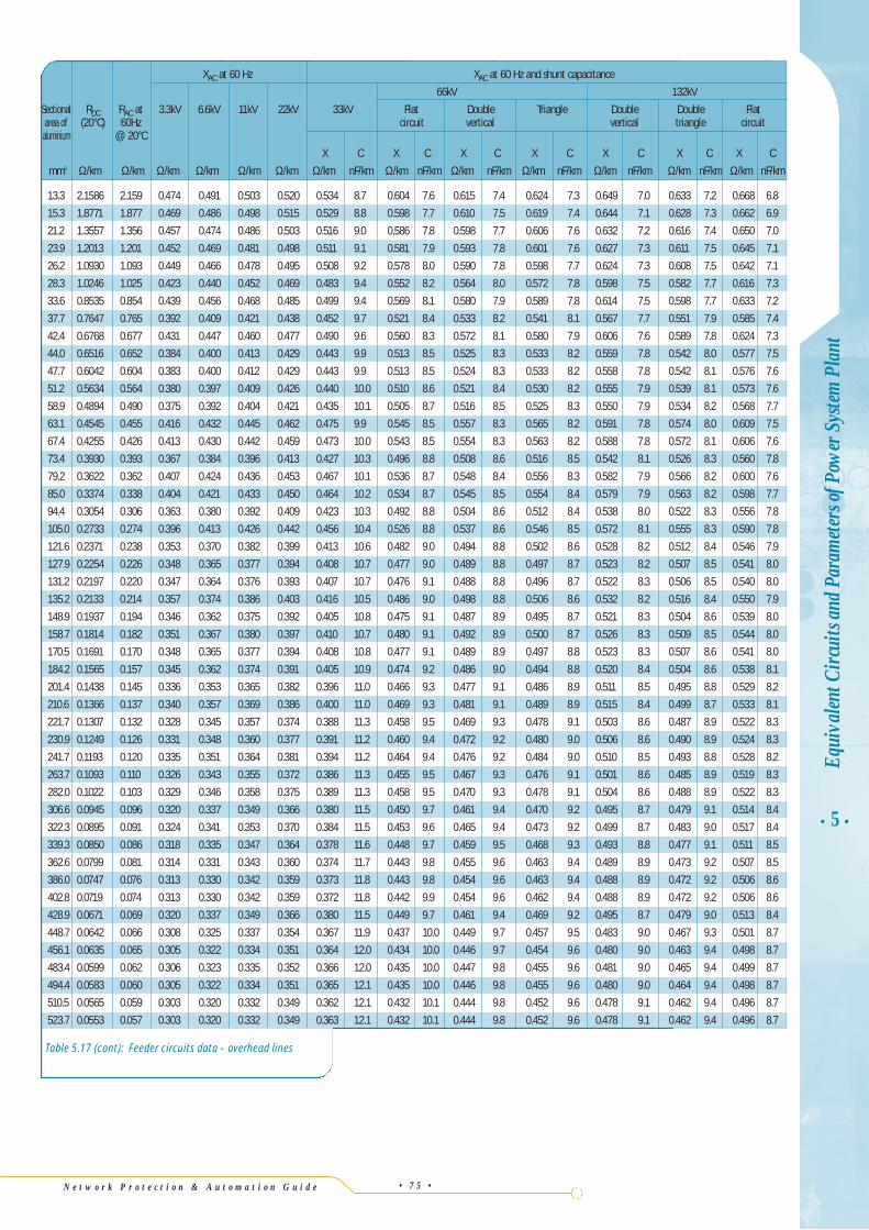
N e t w o r k P r o t e c t i o n & A u t o m a t i o n G u i d e • 7 5 •

• 5 •Eq

uiva

lentC

ircui

tsan

dPar

amete

rsof

Pow

erSy

stem

Plan

t

XAC at 60 Hz XAC at 60 Hz and shunt capacitance

66kV 132kV

Sectional RDC RAC at 3.3kV 6.6kV 11kV 22kV 33kV Flat Double Triangle Double Double Flatarea of (20°C) 60Hz circuit vertical vertical triangle circuit

aluminium @ 20°C

X C X C X C X C X C X C X C

mm2 Ω/km Ω/km Ω/km Ω/km Ω/km Ω/km Ω/km nF/km Ω/km nF/km Ω/km nF/km Ω/km nF/km Ω/km nF/km Ω/km nF/km Ω/km nF/km

13.3 2.1586 2.159 0.474 0.491 0.503 0.520 0.534 8.7 0.604 7.6 0.615 7.4 0.624 7.3 0.649 7.0 0.633 7.2 0.668 6.8

15.3 1.8771 1.877 0.469 0.486 0.498 0.515 0.529 8.8 0.598 7.7 0.610 7.5 0.619 7.4 0.644 7.1 0.628 7.3 0.662 6.9

21.2 1.3557 1.356 0.457 0.474 0.486 0.503 0.516 9.0 0.586 7.8 0.598 7.7 0.606 7.6 0.632 7.2 0.616 7.4 0.650 7.0

23.9 1.2013 1.201 0.452 0.469 0.481 0.498 0.511 9.1 0.581 7.9 0.593 7.8 0.601 7.6 0.627 7.3 0.611 7.5 0.645 7.1

26.2 1.0930 1.093 0.449 0.466 0.478 0.495 0.508 9.2 0.578 8.0 0.590 7.8 0.598 7.7 0.624 7.3 0.608 7.5 0.642 7.1

28.3 1.0246 1.025 0.423 0.440 0.452 0.469 0.483 9.4 0.552 8.2 0.564 8.0 0.572 7.8 0.598 7.5 0.582 7.7 0.616 7.3

33.6 0.8535 0.854 0.439 0.456 0.468 0.485 0.499 9.4 0.569 8.1 0.580 7.9 0.589 7.8 0.614 7.5 0.598 7.7 0.633 7.2

37.7 0.7647 0.765 0.392 0.409 0.421 0.438 0.452 9.7 0.521 8.4 0.533 8.2 0.541 8.1 0.567 7.7 0.551 7.9 0.585 7.4

42.4 0.6768 0.677 0.431 0.447 0.460 0.477 0.490 9.6 0.560 8.3 0.572 8.1 0.580 7.9 0.606 7.6 0.589 7.8 0.624 7.3

44.0 0.6516 0.652 0.384 0.400 0.413 0.429 0.443 9.9 0.513 8.5 0.525 8.3 0.533 8.2 0.559 7.8 0.542 8.0 0.577 7.5

47.7 0.6042 0.604 0.383 0.400 0.412 0.429 0.443 9.9 0.513 8.5 0.524 8.3 0.533 8.2 0.558 7.8 0.542 8.1 0.576 7.6

51.2 0.5634 0.564 0.380 0.397 0.409 0.426 0.440 10.0 0.510 8.6 0.521 8.4 0.530 8.2 0.555 7.9 0.539 8.1 0.573 7.6

58.9 0.4894 0.490 0.375 0.392 0.404 0.421 0.435 10.1 0.505 8.7 0.516 8.5 0.525 8.3 0.550 7.9 0.534 8.2 0.568 7.7

63.1 0.4545 0.455 0.416 0.432 0.445 0.462 0.475 9.9 0.545 8.5 0.557 8.3 0.565 8.2 0.591 7.8 0.574 8.0 0.609 7.5

67.4 0.4255 0.426 0.413 0.430 0.442 0.459 0.473 10.0 0.543 8.5 0.554 8.3 0.563 8.2 0.588 7.8 0.572 8.1 0.606 7.6

73.4 0.3930 0.393 0.367 0.384 0.396 0.413 0.427 10.3 0.496 8.8 0.508 8.6 0.516 8.5 0.542 8.1 0.526 8.3 0.560 7.8

79.2 0.3622 0.362 0.407 0.424 0.436 0.453 0.467 10.1 0.536 8.7 0.548 8.4 0.556 8.3 0.582 7.9 0.566 8.2 0.600 7.6

85.0 0.3374 0.338 0.404 0.421 0.433 0.450 0.464 10.2 0.534 8.7 0.545 8.5 0.554 8.4 0.579 7.9 0.563 8.2 0.598 7.7

94.4 0.3054 0.306 0.363 0.380 0.392 0.409 0.423 10.3 0.492 8.8 0.504 8.6 0.512 8.4 0.538 8.0 0.522 8.3 0.556 7.8

105.0 0.2733 0.274 0.396 0.413 0.426 0.442 0.456 10.4 0.526 8.8 0.537 8.6 0.546 8.5 0.572 8.1 0.555 8.3 0.590 7.8

121.6 0.2371 0.238 0.353 0.370 0.382 0.399 0.413 10.6 0.482 9.0 0.494 8.8 0.502 8.6 0.528 8.2 0.512 8.4 0.546 7.9

127.9 0.2254 0.226 0.348 0.365 0.377 0.394 0.408 10.7 0.477 9.0 0.489 8.8 0.497 8.7 0.523 8.2 0.507 8.5 0.541 8.0

131.2 0.2197 0.220 0.347 0.364 0.376 0.393 0.407 10.7 0.476 9.1 0.488 8.8 0.496 8.7 0.522 8.3 0.506 8.5 0.540 8.0

135.2 0.2133 0.214 0.357 0.374 0.386 0.403 0.416 10.5 0.486 9.0 0.498 8.8 0.506 8.6 0.532 8.2 0.516 8.4 0.550 7.9

148.9 0.1937 0.194 0.346 0.362 0.375 0.392 0.405 10.8 0.475 9.1 0.487 8.9 0.495 8.7 0.521 8.3 0.504 8.6 0.539 8.0

158.7 0.1814 0.182 0.351 0.367 0.380 0.397 0.410 10.7 0.480 9.1 0.492 8.9 0.500 8.7 0.526 8.3 0.509 8.5 0.544 8.0

170.5 0.1691 0.170 0.348 0.365 0.377 0.394 0.408 10.8 0.477 9.1 0.489 8.9 0.497 8.8 0.523 8.3 0.507 8.6 0.541 8.0

184.2 0.1565 0.157 0.345 0.362 0.374 0.391 0.405 10.9 0.474 9.2 0.486 9.0 0.494 8.8 0.520 8.4 0.504 8.6 0.538 8.1

201.4 0.1438 0.145 0.336 0.353 0.365 0.382 0.396 11.0 0.466 9.3 0.477 9.1 0.486 8.9 0.511 8.5 0.495 8.8 0.529 8.2

210.6 0.1366 0.137 0.340 0.357 0.369 0.386 0.400 11.0 0.469 9.3 0.481 9.1 0.489 8.9 0.515 8.4 0.499 8.7 0.533 8.1

221.7 0.1307 0.132 0.328 0.345 0.357 0.374 0.388 11.3 0.458 9.5 0.469 9.3 0.478 9.1 0.503 8.6 0.487 8.9 0.522 8.3

230.9 0.1249 0.126 0.331 0.348 0.360 0.377 0.391 11.2 0.460 9.4 0.472 9.2 0.480 9.0 0.506 8.6 0.490 8.9 0.524 8.3

241.7 0.1193 0.120 0.335 0.351 0.364 0.381 0.394 11.2 0.464 9.4 0.476 9.2 0.484 9.0 0.510 8.5 0.493 8.8 0.528 8.2

263.7 0.1093 0.110 0.326 0.343 0.355 0.372 0.386 11.3 0.455 9.5 0.467 9.3 0.476 9.1 0.501 8.6 0.485 8.9 0.519 8.3

282.0 0.1022 0.103 0.329 0.346 0.358 0.375 0.389 11.3 0.458 9.5 0.470 9.3 0.478 9.1 0.504 8.6 0.488 8.9 0.522 8.3

306.6 0.0945 0.096 0.320 0.337 0.349 0.366 0.380 11.5 0.450 9.7 0.461 9.4 0.470 9.2 0.495 8.7 0.479 9.1 0.514 8.4

322.3 0.0895 0.091 0.324 0.341 0.353 0.370 0.384 11.5 0.453 9.6 0.465 9.4 0.473 9.2 0.499 8.7 0.483 9.0 0.517 8.4

339.3 0.0850 0.086 0.318 0.335 0.347 0.364 0.378 11.6 0.448 9.7 0.459 9.5 0.468 9.3 0.493 8.8 0.477 9.1 0.511 8.5

362.6 0.0799 0.081 0.314 0.331 0.343 0.360 0.374 11.7 0.443 9.8 0.455 9.6 0.463 9.4 0.489 8.9 0.473 9.2 0.507 8.5

386.0 0.0747 0.076 0.313 0.330 0.342 0.359 0.373 11.8 0.443 9.8 0.454 9.6 0.463 9.4 0.488 8.9 0.472 9.2 0.506 8.6

402.8 0.0719 0.074 0.313 0.330 0.342 0.359 0.372 11.8 0.442 9.9 0.454 9.6 0.462 9.4 0.488 8.9 0.472 9.2 0.506 8.6

428.9 0.0671 0.069 0.320 0.337 0.349 0.366 0.380 11.5 0.449 9.7 0.461 9.4 0.469 9.2 0.495 8.7 0.479 9.0 0.513 8.4

448.7 0.0642 0.066 0.308 0.325 0.337 0.354 0.367 11.9 0.437 10.0 0.449 9.7 0.457 9.5 0.483 9.0 0.467 9.3 0.501 8.7

456.1 0.0635 0.065 0.305 0.322 0.334 0.351 0.364 12.0 0.434 10.0 0.446 9.7 0.454 9.6 0.480 9.0 0.463 9.4 0.498 8.7

483.4 0.0599 0.062 0.306 0.323 0.335 0.352 0.366 12.0 0.435 10.0 0.447 9.8 0.455 9.6 0.481 9.0 0.465 9.4 0.499 8.7

494.4 0.0583 0.060 0.305 0.322 0.334 0.351 0.365 12.1 0.435 10.0 0.446 9.8 0.455 9.6 0.480 9.0 0.464 9.4 0.498 8.7

510.5 0.0565 0.059 0.303 0.320 0.332 0.349 0.362 12.1 0.432 10.1 0.444 9.8 0.452 9.6 0.478 9.1 0.462 9.4 0.496 8.7

523.7 0.0553 0.057 0.303 0.320 0.332 0.349 0.363 12.1 0.432 10.1 0.444 9.8 0.452 9.6 0.478 9.1 0.462 9.4 0.496 8.7

Table 5.17 (cont): Feeder circuits data - overhead lines

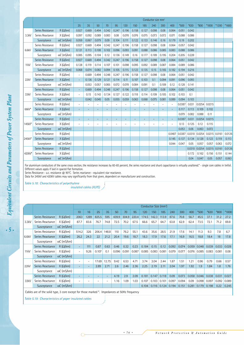
N e t w o r k P r o t e c t i o n & A u t o m a t i o n G u i d e

• 5 •

Equi

valen

tCirc

uits

andP

aram

eters

ofPo

wer

Syste

mPl

ant

• 7 6 •

Conductor size mm2

25 35 50 70 95 120 150 185 240 300 400 *500 *630 *800 *1000 *1200 *1600

Series Resistance R (Ω/km) 0.927 0.669 0.494 0.342 0.247 0.196 0.158 0.127 0.098 0.08 0.064 0.051 0.042

3.3kV Series Reactance X (Ω/km) 0.097 0.092 0.089 0.083 0.08 0.078 0.076 0.075 0.073 0.072 0.071 0.088 0.086

Susceptance ωC (mS/km) 0.059 0.067 0.079 0.09 0.104 0.111 0.122 0.133 0.146 0.16 0.179 0.19 0.202

Series Resistance R (Ω/km) 0.927 0.669 0.494 0.342 0.247 0.196 0.158 0.127 0.098 0.08 0.064 0.057 0.042

6.6kV Series Reactance X (Ω/km) 0.121 0.113 0.108 0.102 0.096 0.093 0.091 0.088 0.086 0.085 0.083 0.088 0.086

Susceptance ωC (mS/km) 0.085 0.095 0.104 0.12 0.136 0.149 0.16 0.177 0.189 0.195 0.204 0.205 0.228

Series Resistance R (Ω/km) 0.927 0.669 0.494 0.342 0.247 0.196 0.158 0.127 0.098 0.08 0.064 0.051 0.042

11kV Series Reactance X (Ω/km) 0.128 0.119 0.114 0.107 0.101 0.098 0.095 0.092 0.089 0.087 0.084 0.089 0.086

Susceptance ωC (mS/km) 0.068 0.074 0.082 0.094 0.105 0.115 0.123 0.135 0.15 0.165 0.182 0.194 0.216

Series Resistance R (Ω/km) - 0.669 0.494 0.348 0.247 0.196 0.158 0.127 0.098 0.08 0.064 0.051 0.042

22kV Series Reactance X (Ω/km) - 0.136 0.129 0.121 0.114 0.11 0.107 0.103 0.1 0.094 0.091 0.096 0.093

Susceptance ωC (mS/km) 0.053 0.057 0.065 0.072 0.078 0.084 0.091 0.1 0.109 0.12 0.128 0.141

Series Resistance R (Ω/km) - 0.669 0.494 0.348 0.247 0.196 0.158 0.127 0.098 0.08 0.064 0.051 0.042

33kV Series Reactance X (Ω/km) - 0.15 0.143 0.134 0.127 0.122 0.118 0.114 0.109 0.105 0.102 0.103 0.1

Susceptance ωC (mS/km) 0.042 0.045 0.05 0.055 0.059 0.063 0.068 0.075 0.081 0.089 0.094 0.103

Series Resistance R (Ω/km) - - - - - - - - - - - 0.0387 0.031 0.0254 0.0215

66kV* Series Reactance X (Ω/km) - - - - - - - - - - - 0.117 0.113 0.109 0.102

Susceptance ωC (mS/km) 0.079 0.082 0.088 0.11

Series Resistance R (Ω/km) - - - - - - - - - - - 0.0387 0.031 0.0254 0.0215

145kV* Series Reactance X (Ω/km) - - - - - - - - - - - 0.13 0.125 0.12 0.115

Susceptance ωC (mS/km) 0.053 0.06 0.063 0.072

Series Resistance R (Ω/km) 0.0487 0.0387 0.0310 0.0254 0.0215 0.0161 0.0126

245kV* Series Reactance X (Ω/km) 0.145 0.137 0.134 0.128 0.123 0.119 0.113

Susceptance ωC (mS/km) 0.044 0.047 0.05 0.057 0.057 0.063 0.072

Series Resistance R (Ω/km) 0.0310 0.0254 0.0215 0.0161 0.0126

420kV* Series Reactance X (Ω/km) 0.172 0.162 0.156 0.151 0.144

Susceptance ωC (mS/km) 0.04 0.047 0.05 0.057 0.063

For aluminium conductors of the same cross-section, the resistance increases by 60-65 percent, the series reactance and shunt capacitance is virtually unaltered.* - single core cables in trefoil.Different values apply if laid in spaced flat formation.Series Resistance - a.c. resistance @ 90°C. Series reactance - equivalent star reactance.Data for 245kV and 420kV cables may vary significantly from that given, dependent on manufacturer and construction.

Table 5.18: Characteristics of polyethyleneinsulated cables (XLPE)

Conductor Size (mm2)

10 16 25 35 50 70 95 120 150 185 240 300 400 *500 *630 *800 *1000

Series Resistance R (Ω/km) 2063 1289 825.5 595 439.9 304.9 220.4 174.5 142.3 113.9 87.6 70.8 56.7 45.5 37.1 31.2 27.2

3.3kV Series Reactance X (Ω/km) 87.7 83.6 76.7 74.8 72.5 70.2 67.5 66.6 65.7 64.7 63.8 62.9 62.4 73.5 72.1 71.2 69.8

Susceptance ωC (mS/km)

Series Resistance R (Ω/km) 514.2 326 206.4 148.8 110 76.2 55.1 43.6 35.6 28.5 21.9 17.6 14.1 11.3 9.3 7.8 6.7

6.6kV Series Reactance X (Ω/km) 26.2 24.3 22 21.2 20.4 19.6 18.7 18.3 17.9 17.6 17.1 16.9 16.5 18.8 18.4 18 17.8

Susceptance ωC (mS/km)

Series Resistance R (Ω/km) - 111 0.87 0.63 0.46 0.32 0.23 0.184 0.15 0.12 0.092 0.074 0.059 0.048 0.039 0.033 0.028

11kV Series Reactance X (Ω/km) - 9.26 0.107 0.1 0.096 0.091 0.087 0.085 0.083 0.081 0.079 0.077 0.076 0.085 0.083 0.081 0.08

Susceptance ωC (mS/km)

Series Resistance R (Ω/km) - - 17.69 12.75 9.42 6.53 4.71 3.74 3.04 2.44 1.87 1.51 1.21 0.96 0.79 0.66 0.57

22kV Series Reactance X (Ω/km) - - 2.89 2.71 2.6 2.46 2.36 2.25 2.19 2.11 2.04 1.97 1.92 1.9 1.84 1.8 1.76

Susceptance ωC (mS/km)

Series Resistance R (Ω/km) - - - - 4.19 2.9 2.09 0.181 0.147 0.118 0.09 0.073 0.058 0.046 0.038 0.031 0.027

33kV Series Reactance X (Ω/km) - - - - 1.16 1.09 1.03 0.107 0.103 0.101 0.097 0.094 0.09 0.098 0.097 0.092 0.089

Susceptance ωC (mS/km) 0.104 0.116 0.124 0.194 0.151 0.281 0.179 0.198 0.22 0.245

Cables are of the solid type, 3 core except for those marked *. Impedances at 50Hz frequency

Table 5.19: Characteristics of paper insulated cables

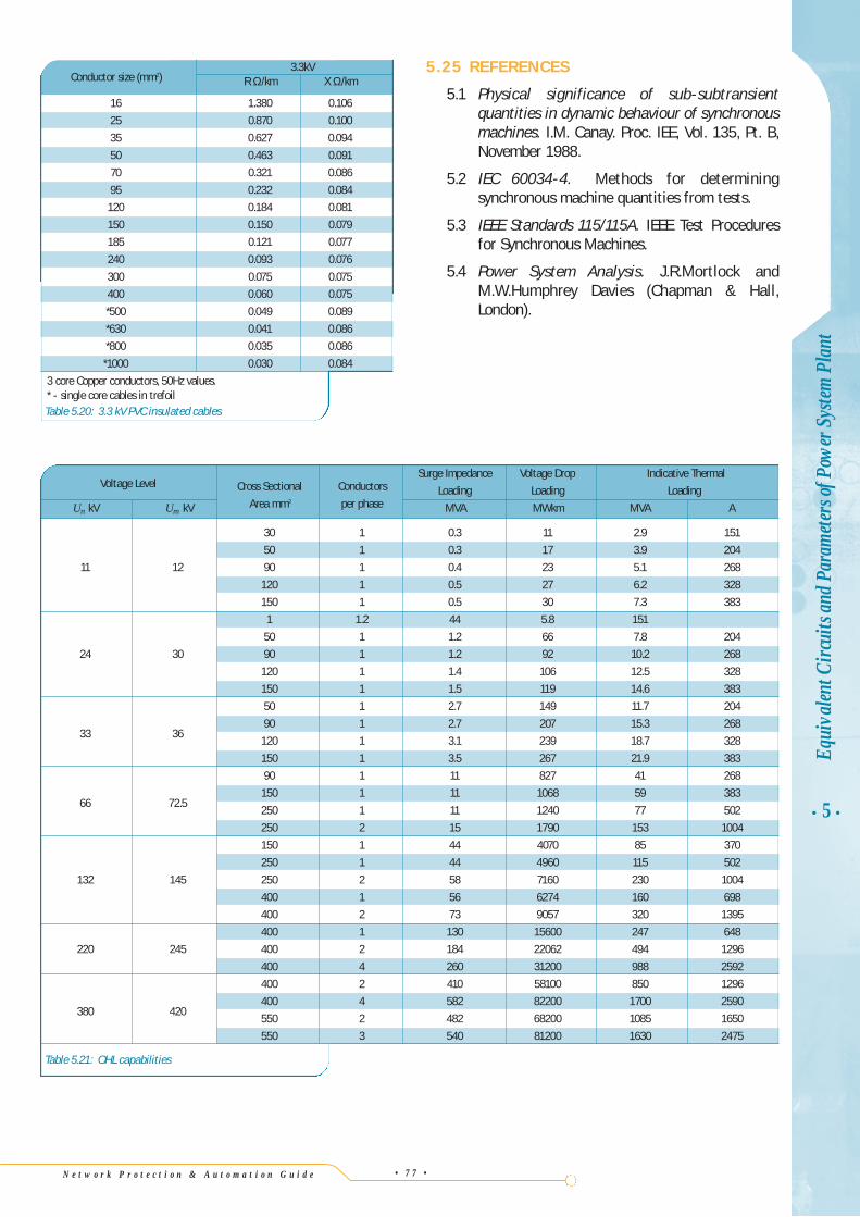
N e t w o r k P r o t e c t i o n & A u t o m a t i o n G u i d e • 7 7 •

• 5 •Eq

uiva

lent C

ircui

ts an

d Par

amete

rs of

Pow

er S

ystem

Pla

nt

5.25 REFERENCES

5.1 Physical significance of sub-subtransientquantities in dynamic behaviour of synchronousmachines. I.M. Canay. Proc. IEE, Vol. 135, Pt. B,November 1988.

5.2 IEC 60034-4. Methods for determiningsynchronous machine quantities from tests.

5.3 IEEE Standards 115/115A. IEEE Test Proceduresfor Synchronous Machines.

5.4 Power System Analysis. J.R.Mortlock andM.W.Humphrey Davies (Chapman & Hall,London).

Conductor size (mm2)3.3kV

R Ω/km X Ω/km

16 1.380 0.106

25 0.870 0.100

35 0.627 0.094

50 0.463 0.091

70 0.321 0.086

95 0.232 0.084

120 0.184 0.081

150 0.150 0.079

185 0.121 0.077

240 0.093 0.076

300 0.075 0.075

400 0.060 0.075

*500 0.049 0.089

*630 0.041 0.086

*800 0.035 0.086

*1000 0.030 0.084

3 core Copper conductors, 50Hz values. * - single core cables in trefoilTable 5.20: 3.3 kV PVC insulated cables

Table 5.21: OHL capabilities

Voltage LevelSurge Impedance Voltage Drop Indicative Thermal

Cross Sectional Conductors Loading Loading Loading

Un kV Um kV Area mm2 per phase MVA MWkm MVA A

30 1 0.3 11 2.9 151

50 1 0.3 17 3.9 204

11 12 90 1 0.4 23 5.1 268

120 1 0.5 27 6.2 328

150 1 0.5 30 7.3 383

1 1.2 44 5.8 151

50 1 1.2 66 7.8 204

24 30 90 1 1.2 92 10.2 268

120 1 1.4 106 12.5 328

150 1 1.5 119 14.6 383

50 1 2.7 149 11.7 204

33 3690 1 2.7 207 15.3 268

120 1 3.1 239 18.7 328

150 1 3.5 267 21.9 383

90 1 11 827 41 268

66 72.5150 1 11 1068 59 383

250 1 11 1240 77 502

250 2 15 1790 153 1004

150 1 44 4070 85 370

250 1 44 4960 115 502

132 145 250 2 58 7160 230 1004

400 1 56 6274 160 698

400 2 73 9057 320 1395

400 1 130 15600 247 648

220 245 400 2 184 22062 494 1296

400 4 260 31200 988 2592

400 2 410 58100 850 1296

380 420400 4 582 82200 1700 2590

550 2 482 68200 1085 1650

550 3 540 81200 1630 2475