5.1 The Nature of Airflow over the surface

Atmospheric Boundary layer (Chapter one) …………………………………..Dr. Ahmed Fattah Hassoon

(1)

Chapter five

(Wind profile)

5.1 The Nature of Airflow over the surface:

The fluid moving over a level surface exerts a horizontal force on the surface

in the direction of motion of the fluid , such a drag force is usually expressed

per unit area of surface and termed shearing stress . conversely , the surface

exerts an equal and opposite retarding force on the fluid this force does not

act on the bulk of the fluid ( at least in the first instance ) but only on its

lower boundary and on a region of more or less restricted extent immediately

above , known as the fluid boundary layer .

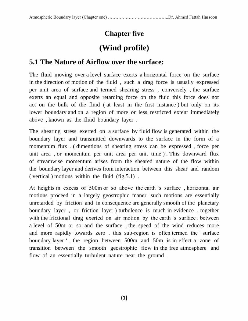
The shearing stress exerted on a surface by fluid flow is generated within the

boundary layer and transmitted downwards to the surface in the form of a

momentum flux . ( dimentions of shearing stress can be expressed , force per

unit area , or momentum per unit area per unit time ) . This downward flux

of streamwise momentum arises from the sheared nature of the flow within

the boundary layer and derives from interaction between this shear and random

( vertical ) motions within the fluid (fig.5.1) .

At heights in excess of 500m or so above the earth ‘s surface , horizontal air

motions proceed in a largely geostrophic maner. such motions are essentially

unretarded by friction and in consequence are generally smooth of the planetary

boundary layer , or friction layer ) turbulence is much in evidence , together

with the frictional drag exerted on air motion by the earth ‘s surface . between

a level of 50m or so and the surface , the speed of the wind reduces more

and more rapidly towards zero . this sub-region is often termed the ‘ surface

boundary layer ‘ . the region between 500m and 50m is in effect a zone of

transition between the smooth geostrophic flow in the free atmosphere and

flow of an essentially turbulent nature near the ground .


(2)

Figure ( 5.1) : Turbulent –boundary –layer flow over a smooth surface .

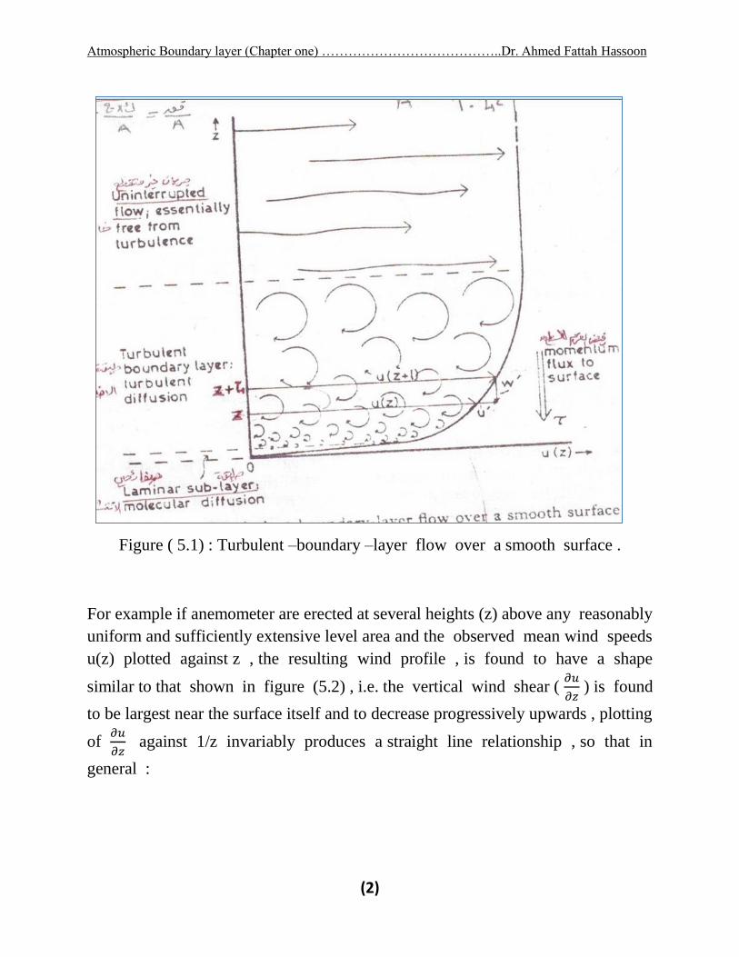
For example if anemometer are erected at several heights (z) above any reasonably

uniform and sufficiently extensive level area and the observed mean wind speeds

u(z) plotted against z , the resulting wind profile , is found to have a shape

similar to that shown in figure (5.2) , i.e. the vertical wind shear ( 𝜕𝑢

𝜕𝑧 ) is found

to be largest near the surface itself and to decrease progressively upwards , plotting

of 𝜕𝑢

𝜕𝑧 against 1/z invariably produces a straight line relationship , so that in

general :


(3)

Figure (5.2) : typical wind profile over a uniform surface .

𝜕𝑢

𝜕𝑧 = 𝐴

1

𝑧 … … … … … … … … … … … … … … … … … (5.1)

Where the parameter A , although independent of z , is a function of wind

speed and of the nature of the surface in question . on integration of equation

5.1 .

𝑢(𝑧) = 𝐴 ln 𝑧 + 𝐵 … … … … … … … … … … … … … … … … . (5.2)

Where B is the appropriate constant of integration . this relationship is of

the form found , in the laboratory , to describe the shape of the wind profile

in a fully developed turbulent boundary layer . thus the nature and characteristics

of airflow close to the earth ‘s surface can be described and explained in

terms of existing boundary layer theory , which has been adequately confirmed

by controlled laboratory experiments .

5.2 Aerodynamic Roughness Length :


(4)

the aerodynamic rourghness length , z0 , is defined as the height where the

wind speed becomes zero . the word aerodynamic comes because the only true

determination of this parameter is from measurement of the wind speed at verious

heights . given observations of wind speed at two or more heights , it is easy to

solve for z0 and u*. graphically , we can easily find z0 by extrapolating the straight

line drawn through the wind speed measurements on a semi-log graph to the

height where �� = 0 ( i.e. , extrapolate the line towards the ordinate axis ) .

Although this roughness length is not equal to the height of the individual roughness

elements on the ground , there is a one –to – one correspondence between those

roughness elements and the aerodynamic roughness length . in other words , once

the aerodynamic roughness length is determined for a particular surface , it does

not change with wind speed , stability , or stress . it can change if the roughness

elements on the surface change such as caused by changes in the height and

coverage of vegetation, manufacture of fences , construction of houses , deforestation

or lumbering , etc.

Lettau ( 1969 ) suggested a method for estimating the aerodynamic roughness

length based on the average vertical extent of the roughness elements ( 𝒉∗) ,

the average vertical cross –section area obtainable to the wind by one element

(𝒔𝒔) , and the lot size per element [ SL =( total ground surface area / number of

elements )] .

𝑧0 = 0.5 ℎ∗ ( 𝑠𝑠

𝑆𝐿 ) … … … … … … … … … … … … … (5.3)

This relationship is acceptable when the roughness elements are evenly spaced

, not too close together , and have similar height and shape .

Kondo and Yamazawa (1986) proposed a similar relationship , where variations

in individual roughness elements were accounted for . let si represent the actual

horizontal surface area occupied by element i , and hi be the height of that

element . if n elements occupy a total area of ST , then the roughness length can

be approximated by :

𝑧0 = 0.25

𝑆𝑇 ∑ ℎ𝑖 𝑠𝑖 … … … … … … … … … … … … … … (5.4)

𝑛

𝑖=1

. these expression have been applied successfully to buildings in cities .

5.3 Displacement Distance : Over land , if the individual roughness elements are packed very closely together

,then the top of those elements begins to act like a displaced surface . for

example , in some forest canopies the trees are close enough together to make a

solid – looking mass of leaves , when viewed from the air . in some cities the

houses are packed close enough together to give a similar effect , namely , the


(5)

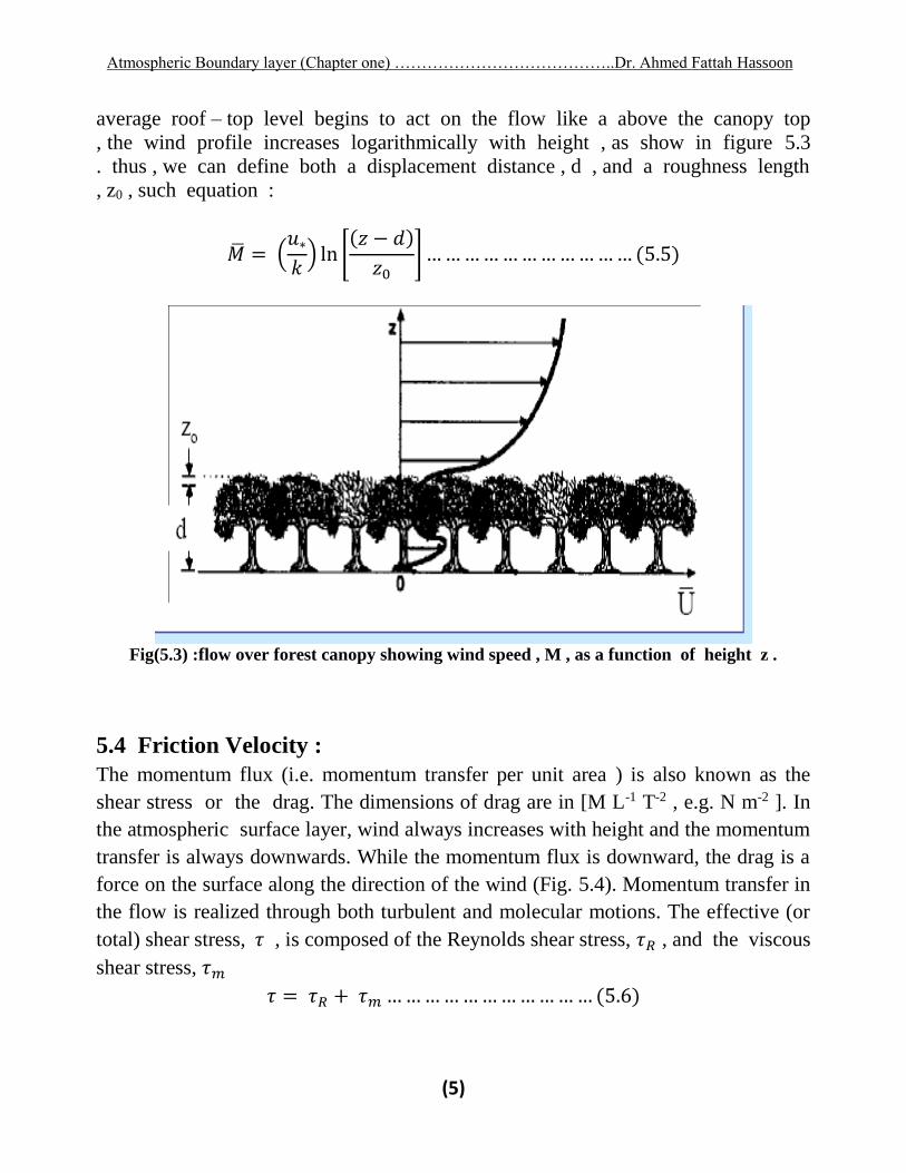
average roof – top level begins to act on the flow like a above the canopy top

, the wind profile increases logarithmically with height , as show in figure 5.3

. thus , we can define both a displacement distance , d , and a roughness length

, z0 , such equation :

�� = (𝑢∗

𝑘) ln [

(𝑧 − 𝑑)

𝑧0] … … … … … … … … … … … (5.5)

Fig(5.3) :flow over forest canopy showing wind speed , M , as a function of height z .

5.4 Friction Velocity :

The momentum flux (i.e. momentum transfer per unit area ) is also known as the

shear stress or the drag. The dimensions of drag are in [M L-1 T-2 , e.g. N m-2 ]. In

the atmospheric surface layer, wind always increases with height and the momentum

transfer is always downwards. While the momentum flux is downward, the drag is a

force on the surface along the direction of the wind (Fig. 5.4). Momentum transfer in

the flow is realized through both turbulent and molecular motions. The effective (or

total) shear stress, 𝜏 , is composed of the Reynolds shear stress, 𝜏𝑅 , and the viscous

shear stress, 𝜏𝑚

𝜏 = 𝜏𝑅 + 𝜏𝑚 … … … … … … … … … … … (5.6)


(6)

The relative importance of 𝜏𝑅 and 𝜏𝑚 depends on the distance from the surface. In

the body of the boundary layer , i.e. above the viscous sub-layer, flows are

predominantly turbulent and, in this region, the momentum flux occurs mainly

through turbulence, and thus is almost identical to 𝜏𝑅 . Closer to the surface,

especially within the viscous layer right next to the surface, the flow is dominated by

viscosity, turbulence is weak and 𝜏𝑅 becomes insignificant. In this region, the

momentum flux occurs mainly through molecular motion. The variations of , 𝜏𝑅 and

𝜏𝑀 with height in the atmospheric boundary layer are as illustrated in Fig. 5.4b.

In the surface layer, 𝜏 remains approximately constant with height. The friction

velocity, 𝑢∗ , is defined as

𝑢∗ = √𝜏

𝜌 … … … … … … … … … … . . (5.7)

Clearly, 𝑢∗ is not the speed of the flow but simply another expression for the

momentum flux at the surface. As 𝑢∗ is a convenient description of the force exerted

on the surface by wind shear, it emerges as one of the most important quantities in

wind-erosion studies. Equation (5.7) can be rewritten as

𝑢∗ = √𝑢′𝑤 ′ ∝ 𝜎 … … … … … … … … … … … … . (5.8)

where 𝜎 is the standard deviation of velocity fluctuations. Thus, 𝑢∗ is also a

descriptor of turbulence intensity in the surface layer and is thus an adequate scaling

velocity for turbulent fluctuations there. Depending upon its characteristics, the

surface can be considered to be dynamically smooth if the sizes of the surface

roughness elements are too small to affect the flow, or otherwise to be dynamically

rough.


(7)

Fig. 5.4. (a) An illustration of mean wind profile in the surface layer. A downward momentum

flux corresponds to shear stress in the direction of the wind. (b) Profiles of effective shear

stress, , Reynolds shear stress, 𝝉𝑹 , and viscous shear stress, 𝝉𝒎 . In the surface layer, 𝝉 = 𝝉𝒎

+ 𝝉𝒓 is approximately constant.

5.5 Shearing Stress via the mixing length concept :

Referring to fig. 5.1, suppose that a lump of fluid originally at the level ( 𝑧 + 𝑙) and

having the appropriate mean velocity 𝑢(𝑧 + 𝑙) is displaced to the level 𝑧 by

the action of turbulence, the instantaneous velocity at 𝑧 then exceeds the mean

value by an amount 𝑢’ given by 𝑢(𝑧 + 𝑙) − 𝑢(𝑧), i.e. to a first approximation .

𝑢′ = 𝑙 ( 𝜕𝑢

𝜕𝑧 ) … … … … … … … … … … … … … … … … . . (5.9)

The subsequent merging of this lump of fluid with its surroundings results in

a quantity of momentum 𝜌𝑢′ per unit volume being contributed to the flow at


(8)

the level 𝑧 . moreover , if the magnitude of the transient vertical velocity

imparted to the lump of fluid is 𝑤’ then the rate at which momentum is

conveyed downwards across unit horizontal area by such a motion must be

𝜌𝑢′𝑤′ . assuming that a constant momentum flux of this magnitude is

communicated by like process to the top of the laminar sub-layer , whence

by molecular means to the surface itself , we may write :

𝜏 = 𝜌 𝑢′𝑤 ′ … … … … … … … … … … … … … … … … … … … … … (5.10)

It is convenient , however to express shearing stress in term of the friction

velocity , 𝑢∗ , such that

𝜏 = 𝜌 𝑢∗2 … … … … … … … … … … … … … … … … … … … … (5.11)

Where 𝑢∗ , like the product 𝑢’𝑤’ , is constant throughout a region of

constant momentum flux , or shearing stress , 𝜏 . if we assume that 𝑢’ and

𝑤’ are merely comparable in size we may deduce that 𝑢∗ is representative

of the magnitude of the velocity fluctuations in turbulent boundary – layer

flow . it is however justifiable to assume equality of 𝑢’ and 𝑤’ , so that .

𝑢′ = 𝑤 ′ = 𝑢∗ … … … … … … … … … … … … … … … … . . (5.12)

The apparently motion of fluid in a turbulent boundary layer may be

visualized on which large numbers of eddies are superimposed , each eddy

moves with the mean flow velocity 𝑢(𝑧) , it is with the scale of these

individual eddies that mixing length can be identified . we expect this scale

to decrease downwards through the boundary layer ( as depicated in figure 5.1

) until , at the surface itself , all turbulent motions are inhibited and 𝑙 = 0.

The simplest possible deduction from this reasoning is that 𝑙 is directly

proportional to distance above the surface - and this is confirmed by experiment

, so that :

𝑙 = 𝑘𝑧 … … … … … … … … … … … … … … … … … . (5.13)

Moreover the constant of proportionality , 𝑘 , is found to be independent of

the nature of the underlying surface , 𝑘 = 0.4 .


(9)

From equation (5.9) , ( 5.12) , ( 5.13) the parameter A in equation (5.1) can

be equated to 𝑢∗

𝑘 i.e. :

𝜕𝑢

𝜕𝑧=

𝑢∗

𝑘 𝑧 … … … … … … … … … … … … … … … (5.14)

By integration

𝑢(𝑧) = 𝑢∗

𝑘ln 𝑧 + 𝐵 … … … … … … … … … … … … … … . . (5.15)

Equation (5.15) describes the shape of the wind profile in turbulent-

boundary layer flow down to the level of the laminar sub-layer , where at

this layer wind speed which it predicts at 𝑧 = 0 , namely 𝑢(0) = −∞ . this

shortcoming is avoided in practice by restricting the zone of application of

equation (5.15) to the region above a level 𝑧0 , where 𝑧0 is defined by the

requirement that 𝑢(𝑧0) = 0 . equation (5.16) then takes the practical form :

𝑢(𝑧) = 𝑢∗

𝑘ln

𝑧

𝑧0… … … … … … … … … … … … … … … (5.16)

In which 𝑧0 includes the role of constant of integration previously held by

B .

5-6 Wind Profile in Statically Neutral Conditions :

To estimate the mean wind speed , �� , as a function of height , z , above the

ground , we speculate that the following variables are relevant : surface stress

( represented by the friction velocity , u* ) , and surface roughness ( represented by

the aerodynamic roughness length , z0 ) . upon applying Buckingham Pi theory , we

find the following two dimensionless groups : ��/𝑢 ∗ and 𝑧

𝑧0 . based on the data

already plotted in figure 5.5, we might expect a logarithmic relasionship between

these two groups:

��

𝑢∗=

1

𝑘ln

𝑧

𝑧0… … … … … … … … … … … . . ( 5.17 )


(10)

Figure 5.5 : typical wind speed profiles vs. static stability ( stable , unstable , neutral ) in

the surface layer

Where 1

𝑘 is a constant of proportionality . as discussed before , the von karman

constant , k , is supposedly a universal constant that is not a function of the flow

nor of the surface . the precise value of this constant has yet to be agreed on ,

but most investigators feel that it is either near k=0.35 , or k=0.4 . for simplicity

, Meterologists often pick a coordinate system aligned with the mean wind direction

near the surface, leaving ��=0 and U=�� . this gives the form of the log wind

profile most often seen in the literature .

𝑈 = (𝑢∗

𝑘) ln (

𝑧

𝑧0) … … … … … … … … … … … … ( 5.18 )


(11)

An alternative derivation of the log wind profile is possible using mixing length

theory . where the momentum flux in the surface layer is :

𝑢′𝑤′ = −𝑘2𝑧2 |𝜕��

𝜕𝑧|

𝜕��

𝜕𝑧… … … … … … … … . . ( 5.19 )

But since the momentum flux is apporoximately constant with height in the

surface layer , 𝑢′𝑤′ (𝑧) = 𝑢∗2 substituting this in to the mixing length expression

and taking the square root of the whole equation gives

𝜕��

𝜕𝑧=

𝑢∗

𝑘𝑧 … … … … … … … … … … . . ( 5.20 )

When this is integrated over height from z=z0 ( where M=0 ) to any height z,

we again arrive at equ. 6.2 .

If we divide both side of 5.20 by [𝑢∗

𝑘𝑧] , we find that the directionless wind

shear 𝑀 is equal to unity in the neutral surface layer .

𝑀 = (𝑘𝑧

𝑢∗)

𝜕��

𝜕𝑧= 1 … … … … … … … … … … . . ( 5.25 )

Assuming horizontal homogeneity (∂/∂x and ∂/∂y = 0), Stationarity (∂/∂t = 0) and that

the divergence of turbulent kinetic energy flux is negligible, and (−𝑢’𝑤’ = 𝑢∗2 )

Equation of TKE can be simplified to 𝑔

��𝑤′𝜃′ + 𝑢∗

2𝜕��

𝜕𝑧− 𝜖 = 0 … … … … … … … … … … . . ( 5.26 )

If we take ∈= 𝑢∗3 /𝜅𝑧 , and In a statically-neutral surface layer, 𝑤′𝜃′ = 0, and an

integration of the above equation gives the logarithmic wind profile.

For stable and unstable situations, the wind profile is modified as illustrated in Fig.

5.5. For the unstable situation, a stronger wind shear occurs near the surface, as

stronger turbulence transfers momentum more efficiently from higher levels to

lower levels and increases the wind speed in the surface layer. The situation for

the stable case is the opposite.


(12)

Proplems

1- used the mixing length (l) and relation to height and also turbulent speed change (u’) at the two

level to drive the logarithmaic equation that used to calcualate wind speed with height at the rural

area and at unstable atmospheric condition

2- when we putting anemometers to measured wind speed over surface coated with grass and at

two level 4m and 12m , the mean record wind speed is u(4m)=5.5m/s , u(12m)=8.5m/s . find

Drag coefficient and shear stress at the level 4m .( used k= 0.4 , z0=0.065m , 𝜌 = 1.2𝑘𝑔

𝑚3 ,

assumed neutral condition ) .

3- In the neutral surface layer, eddy viscosity and mixing length can be expressed as 𝐾𝑚 =𝑘 𝑧 𝑢∗ and 𝑙𝑚 = 𝑘𝑧 . Derive an expression for wind distribution, assuming that the friction

velocity 𝑢∗ = (−𝑢′𝑤′ )1/2is independent of height in this constant-flux .

4- through the field measurement in the rural area and at neutral condition , wind speed at the

height 5m and 10m was u(5m)=9m/s and u(10m)= 15m/s , find the roughness length of

surface in (mm) , at wind speed 5m , taken the eddy height l=0.5m .

5- ( the net momentum flux in the layer near the surface is moved twords the earth surface )

.why? prove that the change in momentum per unit area per unit time is equal to shear stress .(

formulated by physical laws)

6- through the logarithmic equation to change wind speed with height ,at two level z1 and z2

state that :

𝑙𝑛𝑧0 = 𝑢2𝑙𝑛𝑧1 − 𝑢1 ln 𝑧2

𝑢2 − 𝑢1

7- through the engineering application we can calculate the estimate wind speed with height by

depending on power law , that given by : u=zp

8- state that when the friction velocity is constant at two levels , the friction velocity can

putting in :

𝑢∗ = 𝑘 ( 𝑢(𝑧2) − 𝑢(𝑧1))

ln(𝑧2𝑧1

)

9- through the use of logarithms wind speed at two level 𝑧1 , 𝑧2 , state that roughness length

is equal to :

𝑧0 = 𝑧1

(𝑧2𝑧1

)𝑥 𝑤ℎ𝑒𝑟𝑒 𝑥 =

𝑢(𝑧1)

𝑢(𝑧2) − 𝑢(𝑧1)


(13)

5.7 Wind Profile in Non-Neutral Conditions :

Expressions such as 5.18 , 5.26 for statically neutral flow relate the momentum

flux , as described by 𝑢∗2 , to the vertical profile of ��- velocity . those

expressions can be called flux – profile relationship . these relationship can be

extended to include non- neutral ( diabatic ) surface layers , by used Businger – dyer

Relationships. In non- neutral conditions, we might expect that the buoyancy

parameter and the surface heat flux are additional relevant variables. Buckingham Pi

analysis gives us three dimensionless groups ( neglecting the displacement distance

for now ) : ��/u* , z/z0 and z/L , where L is the Obukhov length . alternatively , if

we consider the shear instead of the speed , we get two dimensionless groups

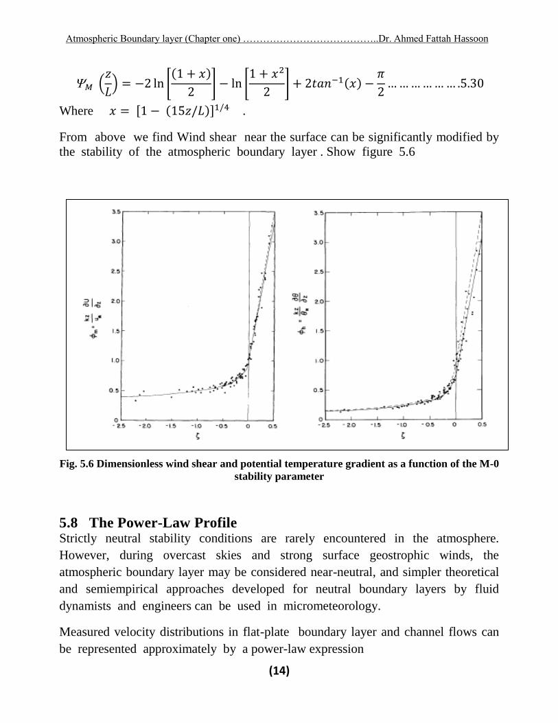
: 𝑴 , and z/L . based on field experiment data , Businger , et .al. , 1971 and dyer

(1974) independently estimated the functional form to be :

𝑀 = 1 + 4.7 𝑧

𝐿 𝑓𝑜𝑟

𝑧

𝐿 > 0 ( 𝑠𝑡𝑎𝑏𝑙𝑒 ) … … … … . .5.27𝑎

𝑀 = 1 𝑓𝑜𝑟 𝑧

𝐿 = 0 ( 𝑛𝑒𝑢𝑡𝑟𝑎𝑙 ) … … … … … … .5.27𝑏

𝑀 = [1 − (15 𝑧

𝐿)]

−1/4

𝑓𝑜𝑟 𝑧

𝐿 < 0 ( 𝑢𝑛𝑠𝑡𝑎𝑏𝑙𝑒 ) … … … .5.27𝑐

These are plotted in fig 5.6 , where Businger, et. al . , have suggested that k=0.35

for their set .

The Businger –Dyer Relationships can be integrated with height to yield the wind

speed profiles .

��

𝑢∗= (

1

𝑘) [ln (

𝑧

𝑧0) + (

𝑧

𝐿)] … … … … … … . . … … … … … 5.28

Where the function (𝑧

𝐿) is give for stable conditions ( z/L > 0 ) by :

(𝑧

𝐿) = 4.7 (

𝑧

𝐿) … … … … … … … … . … … … … … 5.29

And for unstable ( z/L < 0) by :


(14)

𝑀 (𝑧

𝐿) = −2 ln [

(1 + 𝑥)

2] − ln [

1 + 𝑥2

2] + 2𝑡𝑎𝑛−1(𝑥) −

𝜋

2… … … … … … .5.30

Where 𝑥 = [1 − (15𝑧/𝐿)]1/4 .

From above we find Wind shear near the surface can be significantly modified by

the stability of the atmospheric boundary layer . Show figure 5.6

Fig. 5.6 Dimensionless wind shear and potential temperature gradient as a function of the M-0

stability parameter

5.8 The Power-Law Profile Strictly neutral stability conditions are rarely encountered in the atmosphere.

However, during overcast skies and strong surface geostrophic winds, the

atmospheric boundary layer may be considered near-neutral, and simpler theoretical

and semiempirical approaches developed for neutral boundary layers by fluid

dynamists and engineers can be used in micrometeorology.

Measured velocity distributions in flat-plate boundary layer and channel flows can

be represented approximately by a power-law expression


(15)

( 𝑈

𝑈ℎ) = (

𝑧

ℎ)

𝑚

… … … … … … … … . . (5.31)

which was originally suggested by L. Prandtl with an exponent m = 1/7 for smooth

surfaces. Here, h is the boundary layer thickness or half-channel depth. Since, wind

speed does not increase monotonically with height up to the top of the PBL, a slightly

modified version of Equation (5.31) is used in micrometeorology:

( 𝑈

𝑈𝑟) = (

𝑧

𝑧𝑟)

𝑚

… … … … … … … … … . (5.32)

where Ur is the wind speed at a reference height zr, which is smaller than or equal to

the height of wind speed maximum; a standard reference height of 10m is commonly

used.

The power-law profile does not have a sound theoretical basis, but frequently it

provides a reasonable fit to the observed velocity profiles in the lower part of the

PBL, as shown in Figure 5.7. The exponent m is found to depend on both the surface

roughness and stability. Under near-neutral conditions, values of m range from 0.10

for smooth water, snow and ice surfaces to about 0.40 for well-developed urban

areas. Figure 5.8 shows the dependence of m on the roughness length or parameter

z0, which will be defined later. The exponent m also increases with increasing

stability and approaches one (corresponding to a linear profile) under very stable

conditions. The value of the exponent may also depend, to some extent, on the height

range over which the power law is fitted to the observed profile. The power-law

velocity profile implies a power-law eddy viscosity (Km) distribution in the lower part

of the boundary layer, in which the momentum flux may be assumed to remain nearly

constant with height, i.e., in the constant stress layer. It is easy to show that

( 𝐾𝑚

𝐾𝑚𝑟) = (

𝑧

𝑧𝑟)

𝑛

… … … … … … … … . (5.33)

with the exponent n = 1 — m, is consistent with Equation (5.33) in the surface layer.

Equation 5.32 , 5.33 are called conjugate power laws and have been used extensively

in theoretical formulations of atmospheric diffusion , including transfers of heat and

water vapour from extensive uniform surfaces .


(16)

In such formulations eddy diffusivities of heat and mass are assumed to be equal or

proportional to eddy viscosity, and thermodynamic energy and diffusion equations

are solved for prescribed velocity and eddy diffusivity profiles in the above

manner.

Figure 6.5 Comparison of observed wind speed profiles at different sites (z0 is a measure of the

surface roughness) under different stability conditions with the power-law profile. [Data from

Izumi and Caughey (1976).]


(17)

Figure 6.6 : Variations of the power-law exponent with the roughness length for near-neutral

conditions.


(18)

Exercises and Problem

Q1) If an orchard is planted with 1000 trees per square kilometer, where each tree is 4m tall

and has a vertical cross-section area ( effective silhouette to the wind ) of 5m2 , what is the

aerodynamic roughness length ? assume d=0 .

Q2) Given the following wind speed data for a neutral surface layer , find the roughness

length ( z0 ) , displacement distance (d) , and friction velocity ( u* ) :

z ( m) 5 8 10 20 30 50

��( m/s) 3.48 4.43 4.66 5.5 5.93 6.45

Q3) Suppose that the following was observed on a clear night ( no clouds ) over farmland

having z0 = 0.067 m ( assume k= 0.4 ) , L ( Obukhov length = 30m ) , u* = 0.2 m/s . find and plot

�� as a function of height up to 50 m .

Q4)

a) if the displacement distance is zero , find z0 and u* , given the following data in Statically

Neutral conditions at sunset :

Z m 1 3 10 30

M m/s 4.6 6 7.6 9

b) later in the evening at the same site , 𝑤′𝜃′𝑠

= −0.01𝐾𝑚

𝑠 , 𝑎𝑛𝑑

𝑔

𝜃𝑣= 0.0333𝑚 𝑠−1𝐾 . if u*= 0.3

m/s , calculate and plot the wind speed profile ( U vs z ) up to z = 50m .

Q5 ) given : a SBL with z0= 1 cm , 𝜃 ( 𝑎𝑡 𝑧 = 10𝑚 ) = 294 𝐾 , 𝑤′𝜃′𝑆

= −0.02 𝑘 .𝑚

𝑠 , 𝑢∗ =

0.2𝑚

𝑠 , 𝑘 = 0.4 . plot the mean wind speed as a function of height on semi- log graph for

1 ≤ z ≤ 100 m .

Q6 ) given the following wind speeds measured at various heights in a neutral boundary layer

, find the aerodynamic roughness length ( z0 ) , the friction velocity ( u*) , and the shear stress at

the ground ( 𝜏) . what would you estimate the wind speeds to be at 2m and at 10cm above the

ground ? use Semi- log paper . assume that the von karman constant is 0.35 .

Z ( m) 1 4 10 20 50 100 300 500 1000 2000

U ( m/s ) 3.7 5 5.8 6.5 7.4 8 9 9.5 10 10

Q7) consider the flow of air over a housing development with no trees and almost identical

houses . in each city block ( 0.1 km by 0.2 km ) , there are 20 houses, where each house has

nearly a square foundation ( 10m on a side ) and has an average height of 5 m . calculate


(19)

the value of the surface stress acting on this neighborhood when a wind speed of 10 m/s is

measured at a height of 20m above ground in statically neutral conditions . express that

stress in parcels .

Q8) Use the definition of the drag coefficient along with the neutral log- wind profile

equation to prove that 𝐶𝐷𝑁 = 𝑘2𝑙𝑛−2 (𝑧

𝑧0) .

Q9) Using the Businger – Dyer flux – profile relationship for statically stable conditions :

a) Derive an equation for the drag coefficient , CD as a function of the following 4 parameters

z : height above ground , z0 = roughness length , L = Obukhov length , k = Von Karman

length

b) Find the resulting ratio of CD/CDN , where CDN is the neutral drag coefficient .

c) Given z = 10m and z = 10m , calculate and plot CD/CDN for a few different values of stability

: 0< z/l < 1 . how does this compare with fig below:

Q10) given the following wind profile :

Z( m) 0.3 0.7 1 2 10 50 100 1000

U( m/s) 5 6 6.4 7.2 9 10 10.2 10.4

And density 𝜌 = 1.2𝑘𝑔

𝑚. assume the displacement distance d=0 .

a) Find z0

b) Find u*

c) Find the surface stress ( in units of N/m2 ) .

Q11) given the following wind profile in statically neutral conditions :

Z( m) 0.95 3 9.5 30

U( m/s ) 3 4 5 6

Find the numerical value of :

a) z0

b) u*

c) Km at 3m

d) CD

Q12) given the following mean wind speed profile , find the roughness length ( z0 ) and the

friction velocity ( u* ) . assume that the surface layer is statically neutral , and that the

displacement distance d= 0 , use k= 0.35 .

z( m) 1 3 10 20 50 100 500 1000

(M) m/s 3 4 5 5.6 6.4 6.8 7 7


(20)


(21)

Q13) Knowing the shear ( 𝑑��

𝑑𝑧 ) at any height z is sufficient to determine the friction

velocity ( u* ) for a neutral surface layer :

𝑢∗ = 𝑘 𝑧 𝑑��

𝑑𝑧

If , however , you do not know the local shear , but instead know the value of the wind speed

��2 and ��1 at the heights z2 and z1 respectively , then you could use the following alternative

expression to find u* : u*= k Z* ∆��

∆𝑧 , derive the exact expression for Z* .

Q14 ) given the following wind speed data for a neutral surface layer , find the roughness

length ( z0 ) , the displacement distance ( d) , and the friction velocity ( u* ) :

Z ( m) 5 8 10 20 30 50

M ( m/s ) 3.48 4.34 4.66 5.50 5.93 6.45

Q15 )

a) given the following was observed over farmland on an overcast day :

u* = 0.4 m/s , d=0 , ��= 5 m/s at z= 10m , find z0 .

b) suppose that the following was observed on a clear night ( No clouds ) over the same

farmland : L= 30m , u*= 0.2m/s , find �� at z= 1 , 10 and 20 m .

c) plot the wind speed profile from (a) and ( b) on semi-log graph paper .

Q16) given the following data : 𝑤′𝜃′ = 0.2𝑚

𝑠 , 𝑧𝑖 = 500𝑚 ,

𝑔

��=

0.03333𝑚

𝑠𝑘 , 𝑢∗ = 0.2

𝑚

𝑠 , 𝑘 =

0.4 , 𝑧0 = 0.01 , 𝑧 = 6𝑚

find :

a) L ( the Obukhov length )

b) z/L

Q17 ) the wind speed = 3m/s at a height of 4m . the ground surface has a roughness length

of z0= 0.01m . find the value of u* for

a) A convective daytime boundary layer where Ri = -0.5

b) A nocturnal boundary layer where Ri = 0.5 .

Documents

5.1 The Nature of Airflow over the surface