5.1Database System Concepts - 6 th Edition Chapter 5: Advanced SQL Advanced Aggregation Features OLAP

5.1Database System Concepts - 6th Edition

Chapter 5: Advanced SQLChapter 5: Advanced SQL

Advanced Aggregation Features

OLAP


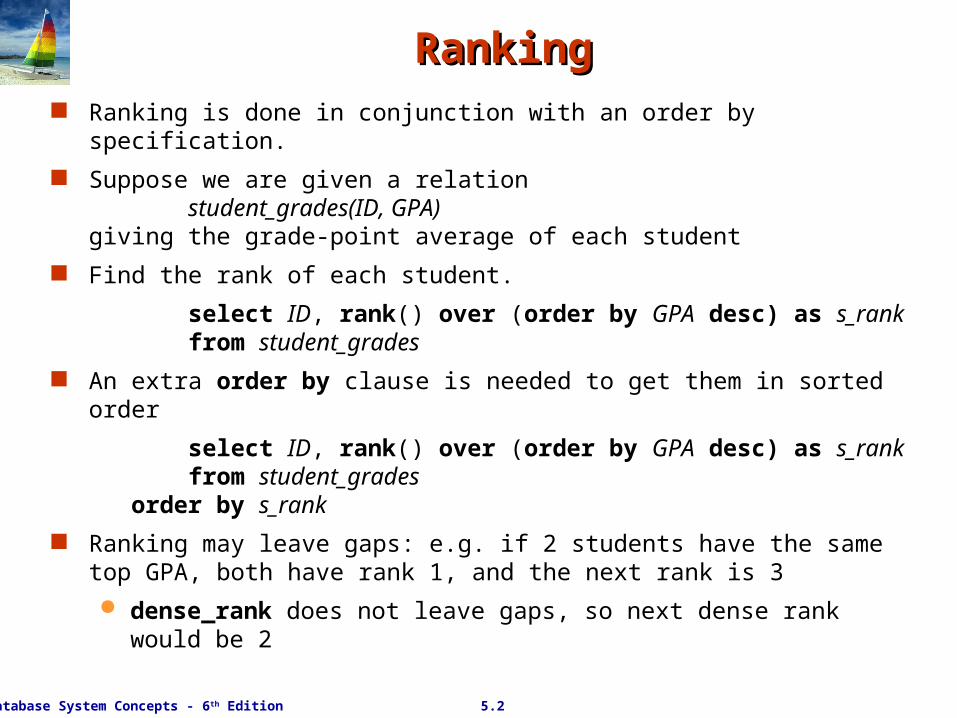
RankingRanking Ranking is done in conjunction with an order by specification.

Suppose we are given a relation student_grades(ID, GPA) giving the grade-point average of each student

Find the rank of each student.

select ID, rank() over (order by GPA desc) as s_rank from student_grades

An extra order by clause is needed to get them in sorted order

select ID, rank() over (order by GPA desc) as s_rank from student_grades order by s_rank

Ranking may leave gaps: e.g. if 2 students have the same top GPA, both have rank 1, and the next rank is 3

dense_rank does not leave gaps, so next dense rank would be 2


Ranking

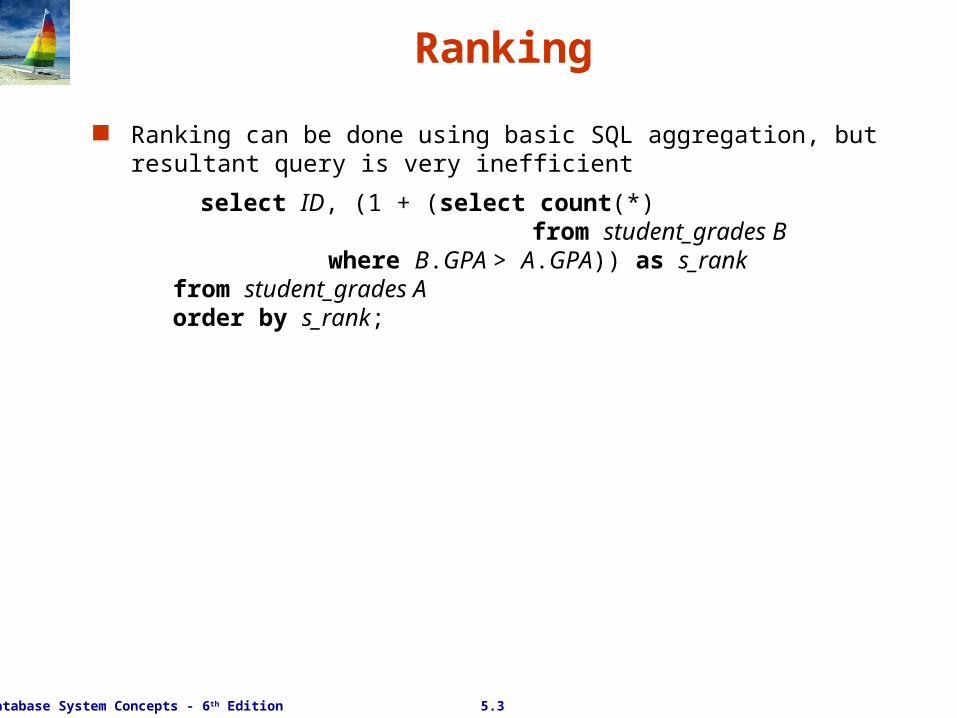
Ranking can be done using basic SQL aggregation, but resultant query is very inefficient

select ID, (1 + (select count(*) from student_grades B where B.GPA > A.GPA)) as s_rankfrom student_grades Aorder by s_rank;


Ranking (Cont.)Ranking (Cont.)

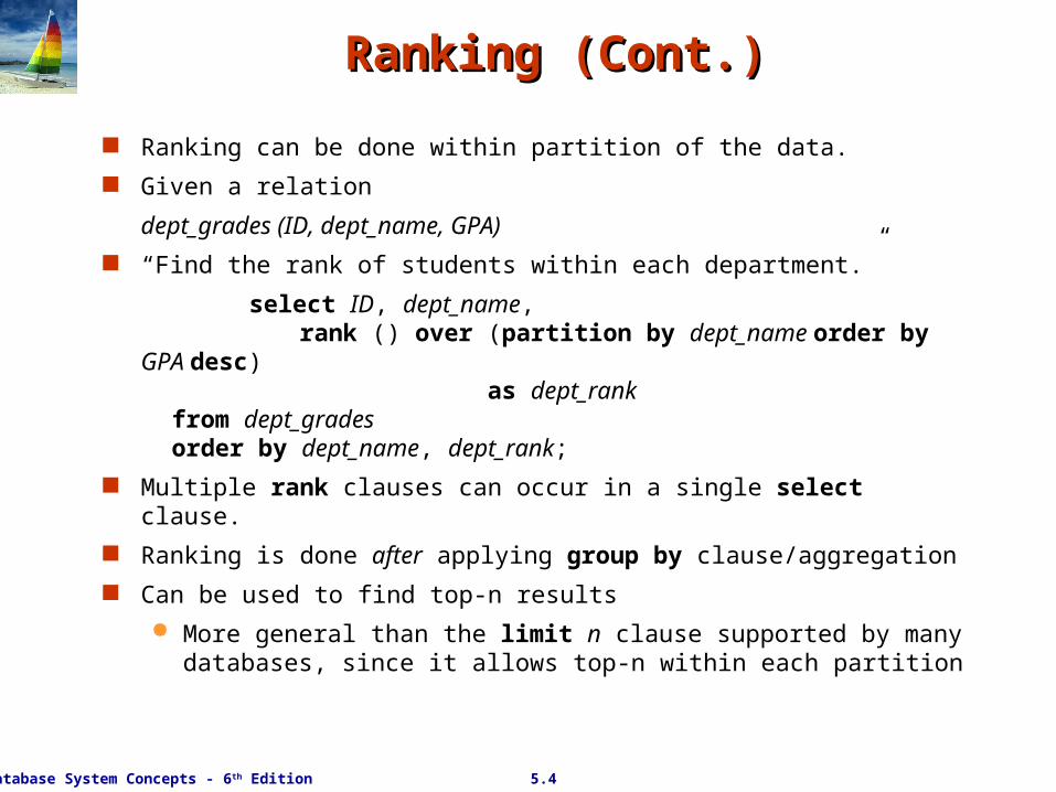
Ranking can be done within partition of the data.

Given a relation

dept_grades (ID, dept_name, GPA)

“Find the rank of students within each department.”

select ID, dept_name, rank () over (partition by dept_name order by GPA desc) as dept_rank from dept_grades order by dept_name, dept_rank;

Multiple rank clauses can occur in a single select clause.

Ranking is done after applying group by clause/aggregation

Can be used to find top-n results

More general than the limit n clause supported by many databases, since it allows top-n within each partition


WindowingWindowing

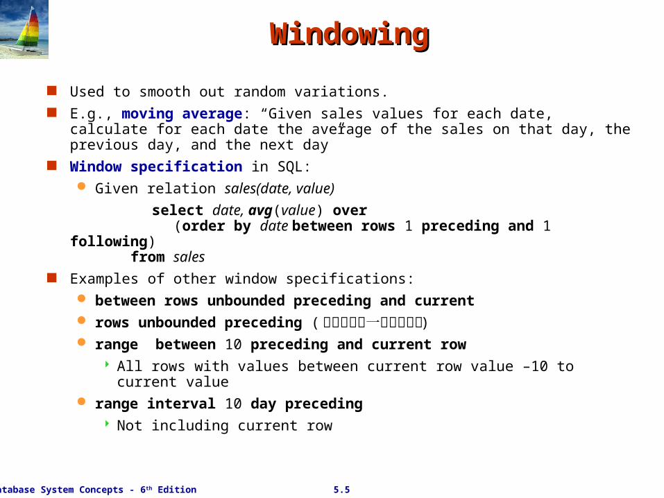
Used to smooth out random variations. E.g., moving average: “Given sales values for each date, calculate for each

date the average of the sales on that day, the previous day, and the next day”

Window specification in SQL: Given relation sales(date, value)

select date, avg(value) over (order by date between rows 1 preceding and 1 following) from sales

Examples of other window specifications: between rows unbounded preceding and current rows unbounded preceding ( 從自己前面一筆到最前面 ) range between 10 preceding and current row

All rows with values between current row value –10 to current value range interval 10 day preceding

Not including current row


Data Analysis and OLAPData Analysis and OLAP

Online Analytical Processing (OLAP)

Interactive analysis of data, allowing data to be summarized and viewed in different ways in an online fashion (with negligible delay)

Data that can be modeled as dimension attributes and measure attributes are called multidimensional data.

For the relation sales(item_name, color, clothes_size, quantify)

Measure attributes

measure some value

can be aggregated upon

e.g., the attribute quantity of the sales relation

Dimension attributes

define the dimensions on which measure attributes (or aggregates thereof) are viewed

e.g., the attributes item_name, color, and clothes_size of the sales relation


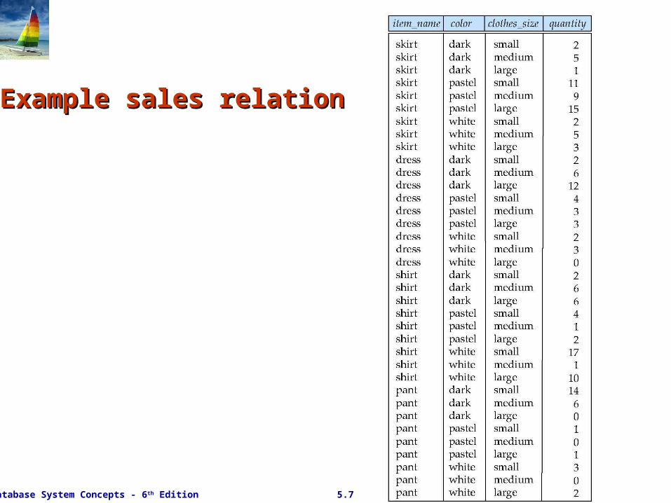
Example sales relation Example sales relation


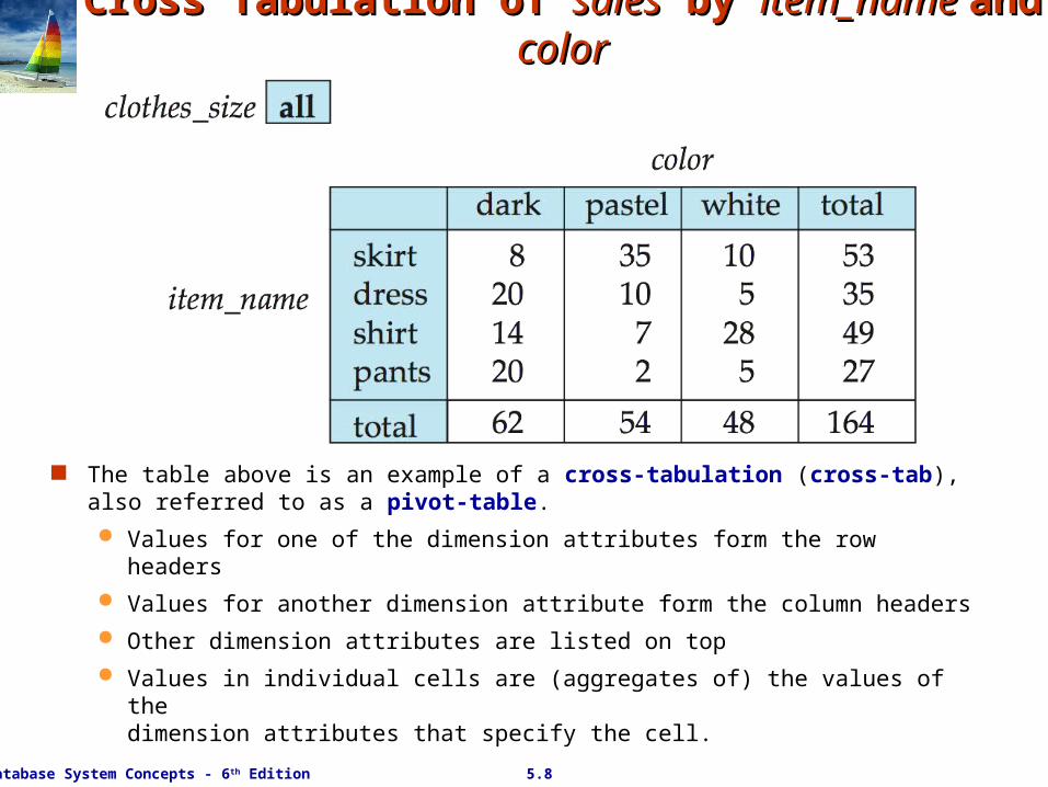
Cross Tabulation of Cross Tabulation of salessales by by item_name item_name and and colorcolor

The table above is an example of a cross-tabulation (cross-tab), also referred to as a pivot-table.

Values for one of the dimension attributes form the row headers

Values for another dimension attribute form the column headers

Other dimension attributes are listed on top

Values in individual cells are (aggregates of) the values of the dimension attributes that specify the cell.


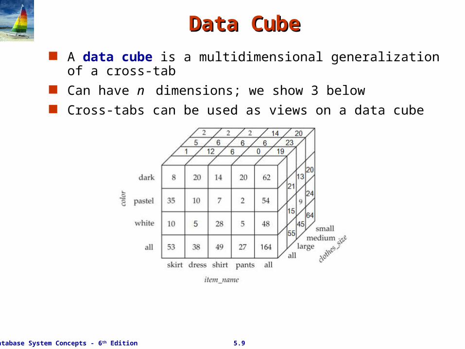
Data CubeData Cube A data cube is a multidimensional generalization of a cross-tab Can have n dimensions; we show 3 below Cross-tabs can be used as views on a data cube


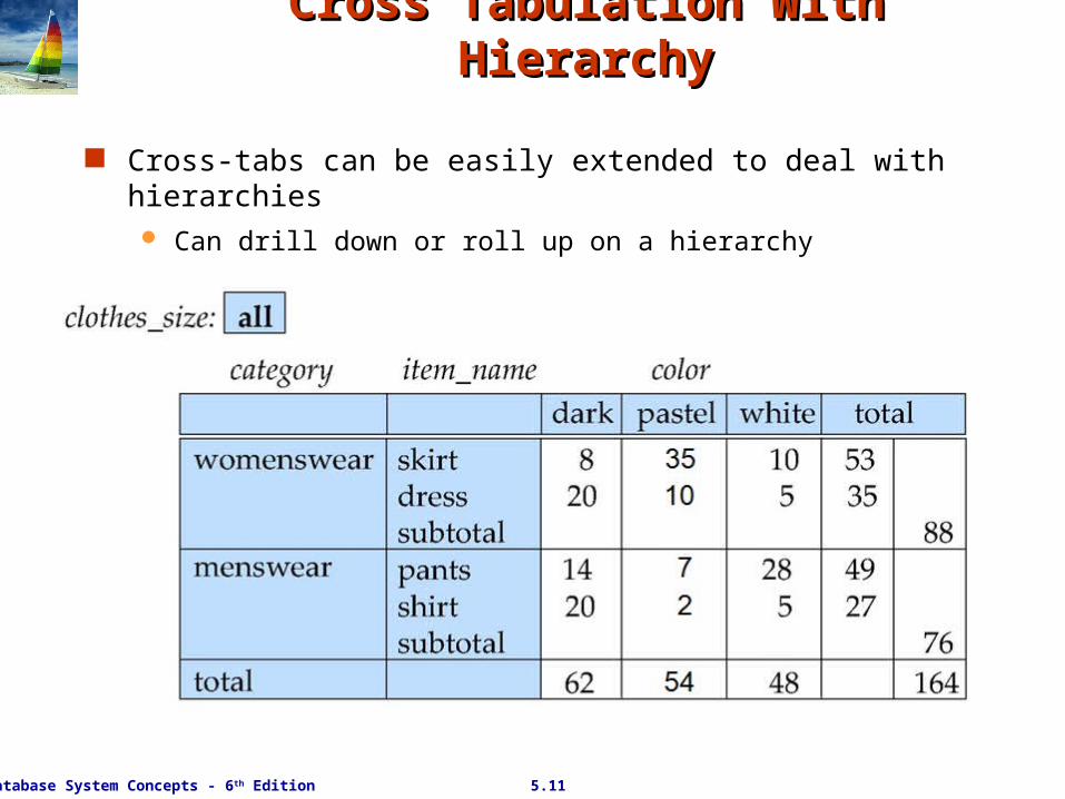
Cross Tabulation With HierarchyCross Tabulation With Hierarchy

Cross-tabs can be easily extended to deal with hierarchies Can drill down or roll up on a hierarchy


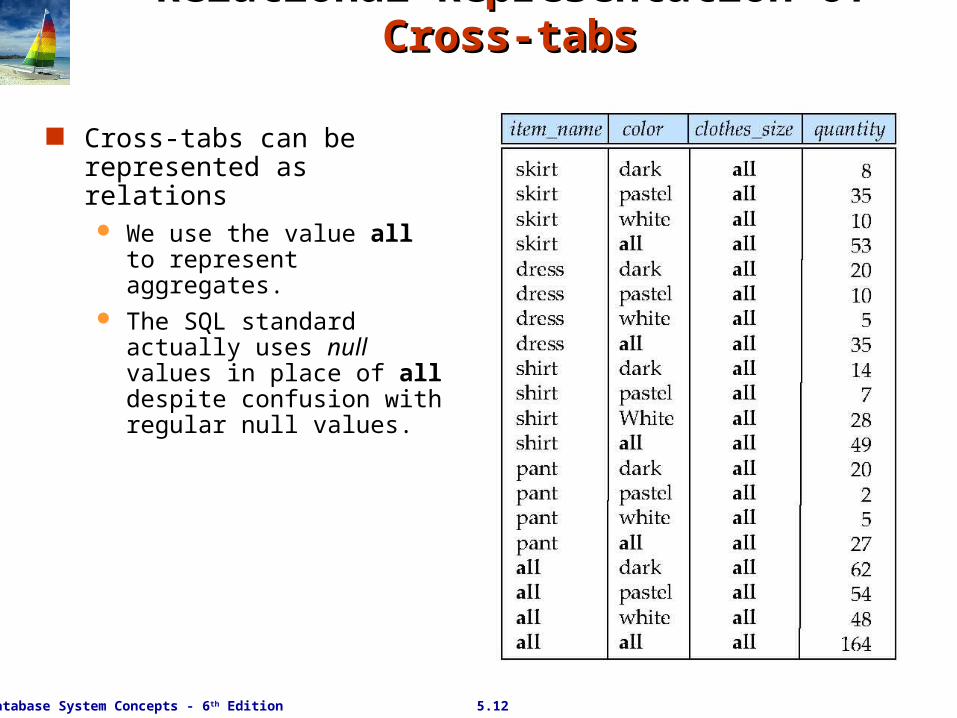
Relational Representation of Cross-tabsRelational Representation of Cross-tabs

Cross-tabs can be represented as relations We use the value all to

represent aggregates. The SQL standard actually

uses null values in place of all despite confusion with regular null values.


Online Analytical Processing OperationsOnline Analytical Processing Operations

Pivoting: changing the dimensions used in a cross-tab

Slicing: creating a cross-tab for fixed values only

Sometimes called dicing, particularly when values for multiple dimensions are fixed.

Rollup: moving from finer-granularity data to a coarser granularity

Drill down: The opposite operation - that of moving from coarser-granularity data to finer-granularity data


Example of “pivot”Example of “pivot”

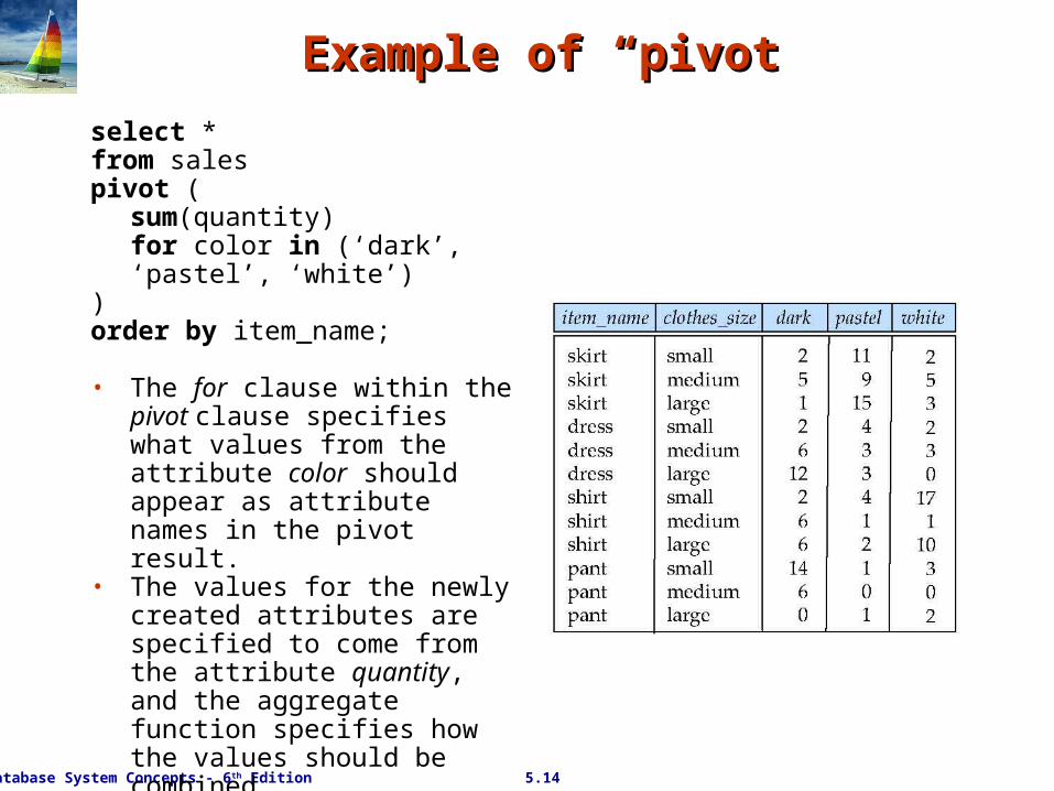
select *from salespivot (

sum(quantity)for color in (‘dark’, ‘pastel’, ‘white’)

)order by item_name;

• The for clause within the pivot clause specifies what values from the attribute color should appear as attribute names in the pivot result.

• The values for the newly created attributes are specified to come from the attribute quantity, and the aggregate function specifies how the values should be combined.


Extended Aggregation to Support OLAPExtended Aggregation to Support OLAP

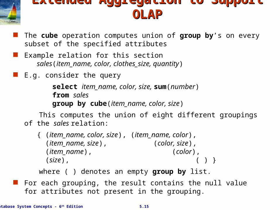
The cube operation computes union of group by’s on every subset of the specified attributes

Example relation for this section sales(item_name, color, clothes_size, quantity)

E.g. consider the query

select item_name, color, size, sum(number)from salesgroup by cube(item_name, color, size)

This computes the union of eight different groupings of the sales relation:

{ (item_name, color, size), (item_name, color), (item_name, size), (color, size), (item_name), (color), (size), ( ) }

where ( ) denotes an empty group by list.

For each grouping, the result contains the null value for attributes not present in the grouping.


Extended Aggregation (Cont.)Extended Aggregation (Cont.)

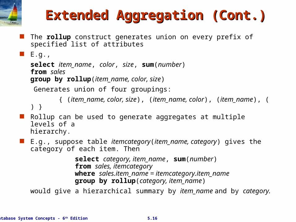
The rollup construct generates union on every prefix of specified list of attributes

E.g.,

select item_name, color, size, sum(number)from salesgroup by rollup(item_name, color, size)

Generates union of four groupings:

{ (item_name, color, size), (item_name, color), (item_name), ( ) } Rollup can be used to generate aggregates at multiple levels of a

hierarchy. E.g., suppose table itemcategory(item_name, category) gives the

category of each item. Then

select category, item_name, sum(number) from sales, itemcategory where sales.item_name = itemcategory.item_name group by rollup(category, item_name)

would give a hierarchical summary by item_name and by category.


Extended Aggregation (Cont.)Extended Aggregation (Cont.)

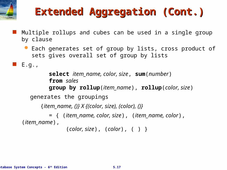
Multiple rollups and cubes can be used in a single group by clause

Each generates set of group by lists, cross product of sets gives overall set of group by lists

E.g.,

select item_name, color, size, sum(number) from sales group by rollup(item_name), rollup(color, size)

generates the groupings

{item_name, ()} X {(color, size), (color), ()}

= { (item_name, color, size), (item_name, color), (item_name), (color, size), (color), ( ) }

Documents

5.1Database System Concepts - 6 th Edition Chapter 5: Advanced SQL Advanced Aggregation Features OLAP