Nature © Macmillan Publishers Ltd 1998

8

of an aplanatic objective lens. Even forbeam tilt angles as high as 30 mrad, the val-ues of defocus and two-fold astigmatisminduced by the residual axial aberrationsremain small.

The basic instrument used for thisdevelopment was a standard 200 kV PhilipsCM 200 ST equipped with a field emissiongun. The corrector increases the columnheight by 24 cm but leaves the other operat-ing modes and functions of the microscopeunaffected. With this modified microscope,we were able to demonstrate the correctionof the spherical aberration and to realize animprovement of the point resolution from0.24 nm to better than 0.14 nm.

The main advantage of spherical aber-ration correction is that structure-imagingartefacts due to contrast delocalization canto a great extent be avoided. These arte-facts have turned out to be a major obsta-cle for the application of instruments withfield emission guns in defect and interfacestudies9. Contrast delocalization arisesfrom the width of the aberration discsbelonging to the individual diffracted elec-tron waves whose diameter increases withthe spherical aberration.

Figure 2a shows, in a cross-sectionalpreparation, the interface of CoSi2 grownepitaxially on Si(111) seen along the<110 > direction. The image was takenunder Scherzer defocus without correction.At the interface, an approximately 2-nm-broad region of darker contrast can beseen. The width depends on the defocusvalue reaching a minimum at the Lichtedefocus10 (Fig. 2b). If the structure isimaged in the aberration-corrected condi-tion (Fig. 2c), the delocalization has essen-tially disappeared and the interface isatomically sharp.Maximilian Haider*, Stephan Uhlemann*,Eugen Schwan European Molecular Biology Laboratory, Postfach 102209, 69012 Heidelberg, Germany*Present address: CEOS GmbH, Im NeuenheimerFeld 519, 69120 Heidelberg, GermanyHarald RoseInstitut für Angewandte Physik, TechnischeHochschule Darmstadt, 64289 Darmstadt, GermanyBernd Kabius, Knut UrbanInstitut für Festkörperforschung,Forschungszentrum Jülich GmbH, 52425 Jülich, Germany

1. Knoll, M. & Ruska, E. Z. Physik 78, 318–339 (1932).

2. Kirkland, E.J. Ultramicroscopy 15, 151–172 (1984).

3. Lichte, H. Ultramicroscopy 20, 293–304 (1986).

4. Scherzer, O. Optik 2, 114–132 (1947).

5. Rose, H. Optik 85, 19–24 (1990).

6. Beck, V.D. Optik 53, 241–255 (1979).

7. Haider, M., Braunshausen, G. & Schwan, E. Optik 99,

167–179 (1995).

8. Zemlin, F., Weiss, K., Schiske, P., Kunath, W. & Herrmann,

K.-H. Ultramicroscopy 3, 49–60 (1977).

9. Thust, A., Coene, W.M.J., Op de Beek, M. & Van Dyck, D.

Ultramicroscopy 64, 211–230 (1996).

10.Lichte, H. Ultramicroscopy 38, 13–22 (1991).

Point vortices exhibitasymmetric equilibria

The equilibrium patterns formed by inter-acting vortices have been puzzled over in avariety of contexts since Kelvin’s theory ofvortex atoms1 was debunked by quantummechanics. These patterns have, for exam-ple, appeared in atmospheric and oceano-graphic flows2,3 and in rotating superfluidhelium4,5. For a particular mathematicalmodel, the point vortex equations, a cata-logue of equilibria was drawn up sometwenty years ago6. We have revisited thepoint vortex model by a different approachand have discovered a host of new equi-librium states, including asymmetric pat-terns devoid of rotational or reflectionalsymmetry.

The dynamical equations considered are

}ddz*t

a} = }2Gpi} }

za–1

zb

} (1)

where the vortices, all of strength G, are par-allel lines that intersect a plane of flow,thought of as the complex plane, at points,za, a = 1,..., N. The asterisk denotes com-plex conjugation; the prime indicates b Þa. For a configuration rotating uniformlywith angular frequency v, za(t) = za(0)eivt,and equation (1) gives the algebraic system:

z*a = }za–

1zb

} (2)

We have rescaled such that 2pv/G = 1.Because of the appearance of complex con-jugation, even determining the total num-ber of solutions of equation (2) for a givenN is not a simple matter.

We now solve equation (2) by a novelnumerical approach. Starting from an equi-librium with N vortices, we first determineall co-rotating points, z, by solving

z* = }z–

1za

} (3)

which we may call Morton’s equation7 as hefirst studied it for N values of 3 and 4.

Given the equilibrium and a co-rotatingpoint, we apply Newton’s method to solvethe system of N + 1 equations

z*a = }za–

1zb

} + }za

e

–z} (4)

for the instantaneous positions a = 1,..., N,together with equation (3), as e variesfrom 0 to 1. This determines an equilibri-um of N + 1 vortices, with N vortices ofstrength 1 and one of strength e, with thesame angular velocity.

N^8b=1

N

a=1

N^8

b=1

N^8b=1

We have no guarantee that solutionsexist continuously in e. Numerical resultsindicate that sometimes, when e is incre-mented, there are no solutions close to theone at hand. When it succeeds, we refer tothis process as ‘growing’ an equilibriumwith N + 1 vortices from one with N vor-tices and a co-rotating point. Similarly, westart with an equilibrium of N + 1 vorticesand gradually reduce the strength of one ofthese from 1 to 0, again solving equations(3) and (4) at every stage with e decrement-ed step by step, until we arrive at an equilib-rium of N vortices and a co-rotating point.

We have also placed ‘seed’ vortices at k > 1 co-rotating points and ‘grown’ a newequilibrium with N + k vortices from onewith N, and we have similarly reduced kvortices step by step in strength from 1 to 0,producing an equilibrium with N – k vor-tices and k co-rotating points. Our methodtends to produce ‘families’ of equilibria,namely similar patterns with different val-ues of N.

By using these procedures, we have dis-covered a large number of new equilibria,many of which depart significantly from thenested-ring type of configuration recordedin the Los Alamos catalogue6. For example,some of our families of configurations are

scientific correspondence

NATURE | VOL 392 | 23 APRIL 1998 769

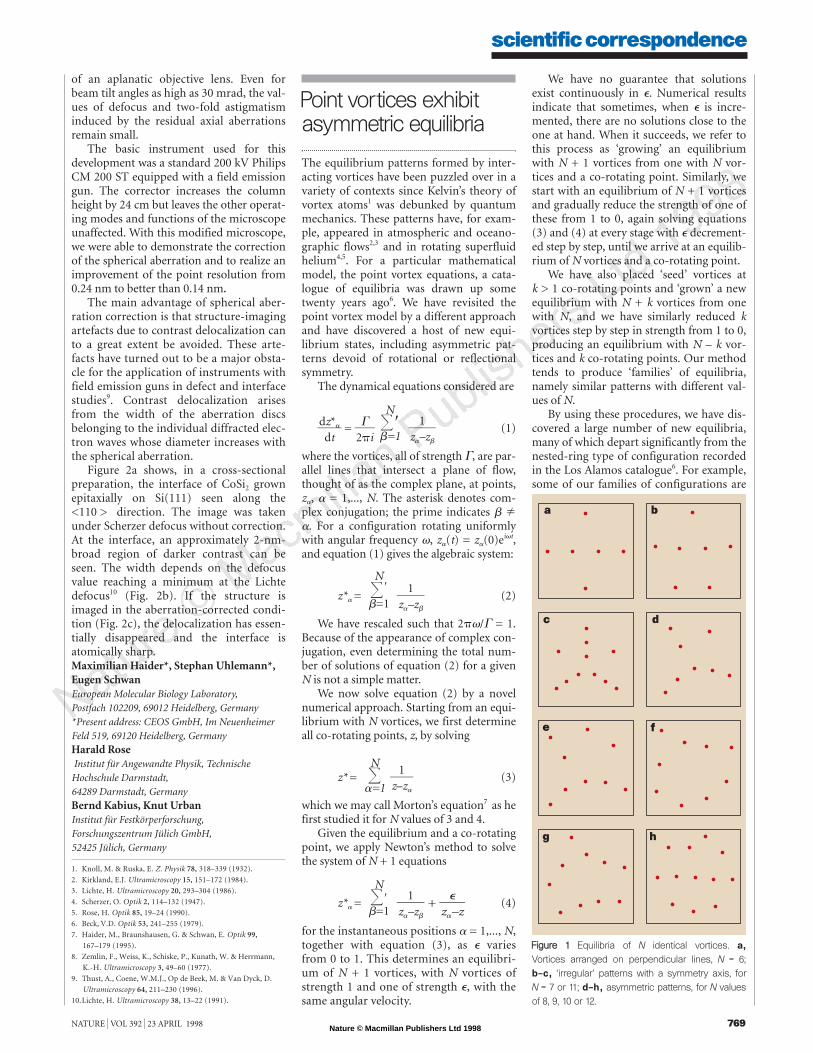
FFiigguurree 11 Equilibria of N identical vortices. a,Vortices arranged on perpendicular lines, N = 6;b–c, ‘irregular’ patterns with a symmetry axis, for N = 7 or 11; d–h, asymmetric patterns, for N valuesof 8, 9, 10 or 12.

a b

c d

e f

g h

Nature © Macmillan Publishers Ltd 1998

8

suggestive of an arrangement along perpen-dicular lines, rather than in rings (Fig.1a; itis possible to determine these analytically);we also found many other irregular config-urations (such as those shown in Fig.1b,c).We stress that in each case the configurationis of the same type for several different val-ues of N, although only one value of N hasbeen shown here.

We have also revealed many new vortexpatterns of the symmetrical, nested-ringtype. All of these have so far turned out tobe unstable, but their number and geomet-ric richness has surprised us.

Finally, and most importantly, we haveidentified equilibria that have no rotationalor reflectional symmetry at all. Examplesfor N values of 8, 9, 10 and 12 are shown inFig.1d–h, but we believe that such equilibriaexist for all N ≥ 8 (and we have found themfor N values of 8–14). Note that the reflec-tion of any of these patterns yields a newequilibrium.

These asymmetric equilibria appear tobelong to several families, and we haveestablished relations among some pairs ofequilibria for different N by the method ofgrowing and reducing equilibria that wedescribe here.

In a non-dissipative system, such aspoint vortices, unstable equilibria play animportant role in determining system evo-lution: as such states are approached, evolu-tion slows down. The existence of unstable,asymmetric equilibria suggests that suchconfigurations will often be observed whena vortex system is started from general ini-tial conditions.Hassan Aref, Dmitri L. VainchteinDepartment of Theoretical and Applied Mechanics,University of Illinois at Urbana-Champaign,216 Talbot Laboratory, 104 South Wright Street,Urbana, Illinois 61801, USA

1. Thomson, W. Nature 18, 13–14 (1878).

2. Stewart, H. J. Q. J. Appl. Math. 1, 262–267 (1943).

3. Carnevale, G. F. & Kloosterziel, R. C. J. Fluid Mech. 259,

305–331 (1995).

4. Williams, G. A. & Packard, R. E. Phys. Rev. Lett. 33, 280–283

(1974).

5. Yarmchuk, E. J., Gordon, M. J. V. & Packard, R. E. Phys. Rev.

Lett. 43, 214–217 (1979).

6. Campbell, L. J. & Ziff, R. M. Los Alamos Sci. Lab. Rep. LA-7384-

MS (1978).

7. Morton, W. B. Proc. R. Irish Acad. A 41, 94–101 (1933).

Scrapie infectivity foundin resistant species

Experimental and epidemiological evidenceindicates that bovine spongiform enceph-alopathy (BSE) has been transmitted tohumans1–4, although the mechanism of thistransmission is unknown. Hamsters andchickens are clinically resistant to the trans-mission of BSE, but we report results thatraise concern over the possible long-term

persistence of infectivity in such clinicallyresistant species and which may have impli-cations for the control of BSE.

‘Natural’ transmission of BSE seems toresult mainly, if not solely, from feedinganimals with meat and bonemeal derivedfrom BSE-infected cattle5. BSE is transmis-sible by inoculation or ingestion to mice,sheep, goats, marmosets, mink, pigs, certainmembers of the cat family and various exot-ic ungulates.

Interestingly, though, it is not transmis-sible to hamsters or chickens5. This resis-tance to BSE is borne out by an absence ofclinical brain disease and a lack of the hall-mark protease-resistant prion protein.

We injected 107 ID50 (where ID50 is thehalf-maximal infectious dose) units ofhamster scrapie agent (strain 263K) into thebrains of groups of C57BL/10 mice thateither did or did not express the mousegene that encodes the normal version of theprion protein (PrP). Mice are highly resis-tant to this hamster scrapie strain6 and, asexpected, none of our mice developed anyclinical symptoms of scrapie.

We found, however, that brain andspleen tissue from the PrP-positive miceobtained between 204 and 782 days afterinoculation contained scrapie agent thatwas capable of infecting hamsters but notmice (Table 1). All of the recipient ham-sters were positive, although the long incu-bation periods indicated that the amountof infectivity present was about 102 ID50

per gram of tissue, far lower than is typi-cally found in clinical scrapie in hamstersor mice.

By contrast, tissues of mice without afunctional PrP gene (PrPo/omice) were onlyvery rarely able to transmit disease to recip-ient hamsters. Thus, expression of a normalmouse PrP gene seemed to enable hamster

scrapie agent to persist in the brains andspleens of normal mice, suggesting that per-haps mouse PrP could be functioning as areceptor for the infectious agent4. However,there was no evidence for any replication ofthe hamster scrapie agent in these persis-tently infected mice. The infectivity recov-ered remained specific for hamsters ratherthan mice (Table 1).

Although we have not tested whethersimilar results would be obtained after oralingestion, this unexpected and prolongedsurvival of a foreign scrapie agent raisesthe possibility that BSE infectivity mightpersist in various ‘resistant’ speciesexposed to BSE-contaminated feeds. Ofparticular concern would be domestic ani-mals such as poultry which are raised forhuman consumption.

So far, there is no evidence for the sec-ondary transmission of BSE from suchresistant species to more susceptiblespecies. However, the results presented herewould strongly favour a decision to stopfeeding ruminant-derived products to allanimal species. Additional experimentsshould be carried out to detect possibleBSE infectivity in clinically normal BSE-exposed animal species. Titration in cattlemay be necessary to achieve the sensitivityneeded to detect the levels of BSE anticipat-ed in such situations.Richard Race, Bruce ChesebroLaboratory of Persistent Viral Diseases,National Institute of Allergy and Infectious Diseases,Hamilton, Montana 59840, USAe-mail: bchesebro@nih.gov

1. Will, R. G. et al. Lancet 347, 921–925 (1996).

2. Bruce, M. E. et al. Nature 389, 498–501 (1997).

3. Hill, A. F. et al. Nature 389, 448–450 (1997).

4. Chesebro, B. Science 279, 42–43 (1998).

5. Collee J. G. & Bradley, R. Lancet 349, 636–641 (1997).

6. Kimberlin, R. H. et al. J.Gen.Virol. 70, 2017–2025 (1989).

7. Manson, J. C. Mol. Neurobiol. 8, 121–127 (1994).

scientific correspondence

770 NATURE | VOL 392 | 23 APRIL 1998

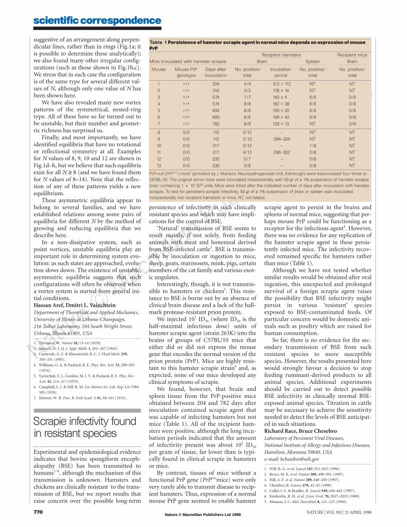
Table 1 Persistence of hamster scrapie agent in normal mice depends on expression of mousePrP

Recipient hamsters Recipient miceMice inoculated with hamster scrapie Brain Spleen Brain

Mouse Mouse PrP Days after No. positive/ Incubation No. positive/ No. positive/genotype inoculation total period total total

1 +/+ 204 4/4 313 ± 112 NT NT

2 +/+ 310 3/3 178 ± 14 NT NT

3 +/+ 574 7/7 140 ± 4 6/6 0/8

4 +/+ 574 8/8 162 ± 38 6/6 0/8

5 +/+ 693 8/8 156 ± 20 6/6 0/8

6 +/+ 693 8/8 168 ± 42 6/6 0/8

7 +/+ 782 8/8 128 ± 13 NT 0/8

8 0/0 112 0/12 — NT NT

9 0/0 112 2/12 294–334 NT NT

10 0/0 217 0/12 — 1/8 NT

11 0/0 217 4/12 296–352 0/8 NT

12 0/0 330 0/7 — 0/8 NT

13 0/0 330 0/8 — 0/8 NT

PrP-null (PrP o/o ) mice7 (provided by J. Manson, Neuropathogenesis Unit, Edinburgh) were backcrossed four times toC57BL/10. The original donor mice were inoculated intracerebrally with 50 µl of a 1% suspension of hamster scrapiebrain containing 1 2 107 ID50 units. Mice were killed after the indicated number of days after inoculation with hamsterscrapie. To test for persistent scrapie infectivity, 50 µl of a 1% suspension of brain or spleen was inoculatedintracerebrally into recipient hamsters or mice. NT, not tested.