1

Digital Filters (Part II)

Cannon (Discrete Systems))

© 2016 School of Information Technology and Electrical Engineering at The University of Queensland

TexPoint fonts used in EMF.

Read the TexPoint manual before you delete this box.: AAAAA

http://elec3004.com

Lecture Schedule:

14 April 2016 ELEC 3004: Systems 2

Week Date Lecture Title

29-Feb Introduction

3-Mar Systems Overview

7-Mar Systems as Maps & Signals as Vectors

10-Mar Data Acquisition & Sampling

14-Mar Sampling Theory

17-Mar Antialiasing Filters

21-Mar Discrete System Analysis

24-Mar Convolution Review

28-Mar

31-Mar

4-Apr Frequency Response & Filter Analysis

7-Apr Filters

11-Apr Digital Filters

14-Apr Digital Filters18-Apr Digital Windows

21-Apr FFT

25-Apr Holiday

28-Apr Feedback

3-May Introduction to Feedback Control

5-May Servoregulation/PID

9-May Introduction to (Digital) Control

12-May Digitial Control

16-May Digital Control Design

19-May Stability

23-May Digital Control Systems: Shaping the Dynamic Response & Estimation

26-May Applications in Industry

30-May System Identification & Information Theory

2-Jun Summary and Course Review

Holiday

1

13

7

8

9

10

11

12

6

2

3

4

5

2

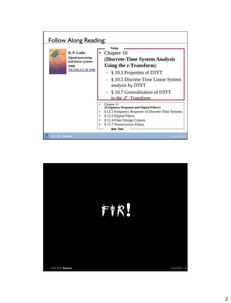
Follow Along Reading:

B. P. Lathi

Signal processing

and linear systems

1998

TK5102.9.L38 1998

• Chapter 10

(Discrete-Time System Analysis

Using the z-Transform)

– § 10.3 Properties of DTFT

– § 10.5 Discrete-Time Linear System

analysis by DTFT

– § 10.7 Generalization of DTFT

to the 𝒵 –Transform

• Chapter 12 (Frequency Response and Digital Filters)

• § 12.1 Frequency Response of Discrete-Time Systems

• § 12.3 Digital Filters

• § 12.4 Filter Design Criteria

• § 12.7 Nonrecursive Filters

Today

14 April 2016 ELEC 3004: Systems 3

!

14 April 2016 ELEC 3004: Systems 4

3

• How to get all these coefficients?

FIR Design Methods:

1. Impulse Response Truncation + Simplest

– Undesirable frequency domain-characteristics, not very useful

2. Windowing Design Method + Simple

– Not optimal (not minimum order for a given performance level)

3. Optimal filter design methods + “More optimal”

– Less simple…

** FIR Filter Design **

14 April 2016 ELEC 3004: Systems 5

• Set Impulse response (order n = 21)

• “Determine” h(t) – h(t) is a 20 element vector that we’ll use to as a weighted sum

• FFT (“Magic”) gives Frequency Response & Phase

FIR Filter Design & Operation Ex: Lowpass FIR filter

14 April 2016 ELEC 3004: Systems 6

4

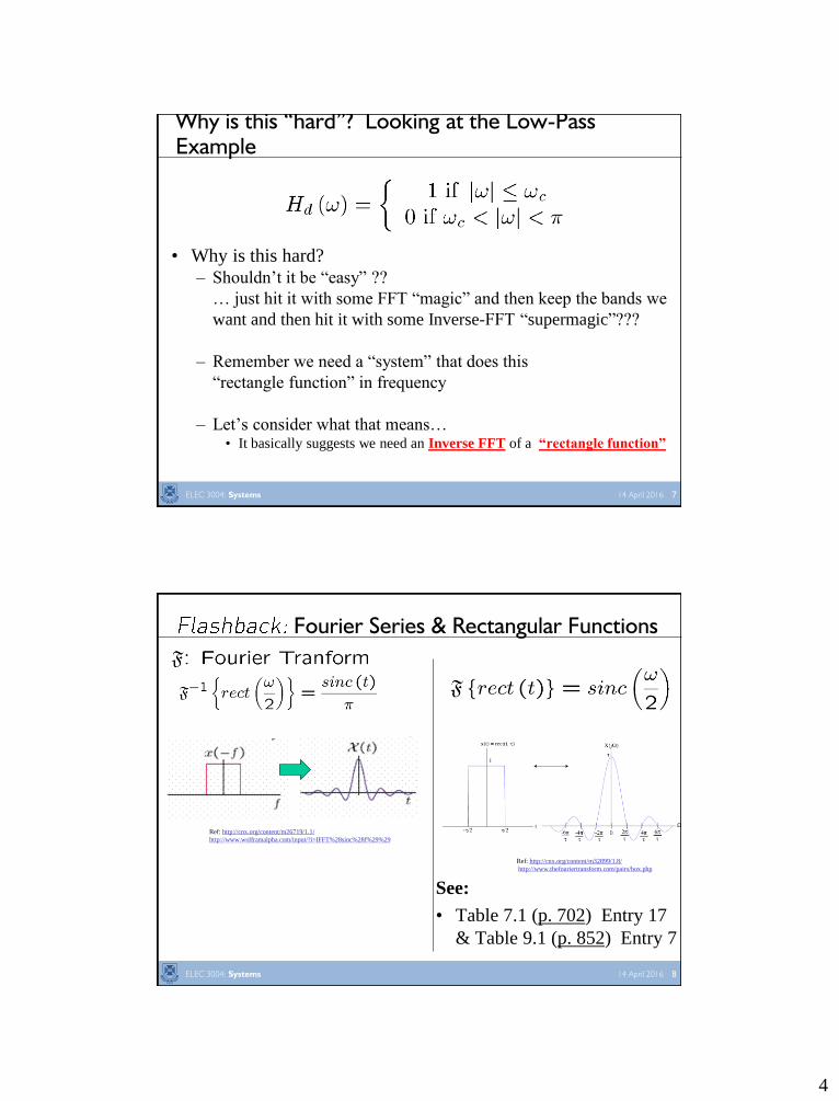
• Why is this hard? – Shouldn’t it be “easy” ??

… just hit it with some FFT “magic” and then keep the bands we

want and then hit it with some Inverse-FFT “supermagic”???

– Remember we need a “system” that does this

“rectangle function” in frequency

– Let’s consider what that means… • It basically suggests we need an Inverse FFT of a “rectangle function”

Why is this “hard”? Looking at the Low-Pass Example

14 April 2016 ELEC 3004: Systems 7

Fourier Series & Rectangular Functions

See:

• Table 7.1 (p. 702) Entry 17

& Table 9.1 (p. 852) Entry 7

Ref: http://cnx.org/content/m32899/1.8/

http://www.thefouriertransform.com/pairs/box.php

Ref: http://cnx.org/content/m26719/1.1/

http://www.wolframalpha.com/input/?i=IFFT%28sinc%28f%29%29

14 April 2016 ELEC 3004: Systems 8

5

• The function might look familiar – This is the frequency content of a square wave (box)

• This also applies to signal reconstruction!

Whittaker–Shannon interpolation formula – This says that the “better way” to go from Discrete to Continuous

(i.e. D to A) is not ZOH, but rather via the sinc!

Fourier Series & Rectangular Functions [2]

Ref: http://www.wolframalpha.com/input/?i=FFT%28rect%28t%29%29

http://cnx.org/content/m32899/1.8/

14 April 2016 ELEC 3004: Systems 9

∴ FIR and Low Pass Filters… ∴

Has impulse response:

Thus, to filter an impulse train

with an ideal low-pass filter use:

• However!!

a is non-causal and

infinite in duration

And, this cannot be

implemented in practice

∵ we need to know all samples of the

input, both in the past and in the future

14 April 2016 ELEC 3004: Systems 10

6

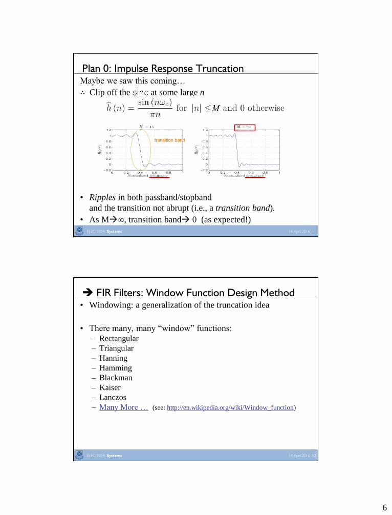
Maybe we saw this coming…

∴ Clip off the at some large n

• Ripples in both passband/stopband

and the transition not abrupt (i.e., a transition band).

• As M∞, transition band 0 (as expected!)

Plan 0: Impulse Response Truncation

14 April 2016 ELEC 3004: Systems 11

• Windowing: a generalization of the truncation idea

• There many, many “window” functions: – Rectangular

– Triangular

– Hanning

– Hamming

– Blackman

– Kaiser

– Lanczos

– Many More … (see: http://en.wikipedia.org/wiki/Window_function)

FIR Filters: Window Function Design Method

14 April 2016 ELEC 3004: Systems 12

7

1. Rectangular

Some Window Functions [1]

14 April 2016 ELEC 3004: Systems 13

Windowing and its effects/terminology

Lathi, Fig. 7.45

14 April 2016 ELEC 3004: Systems 14

8

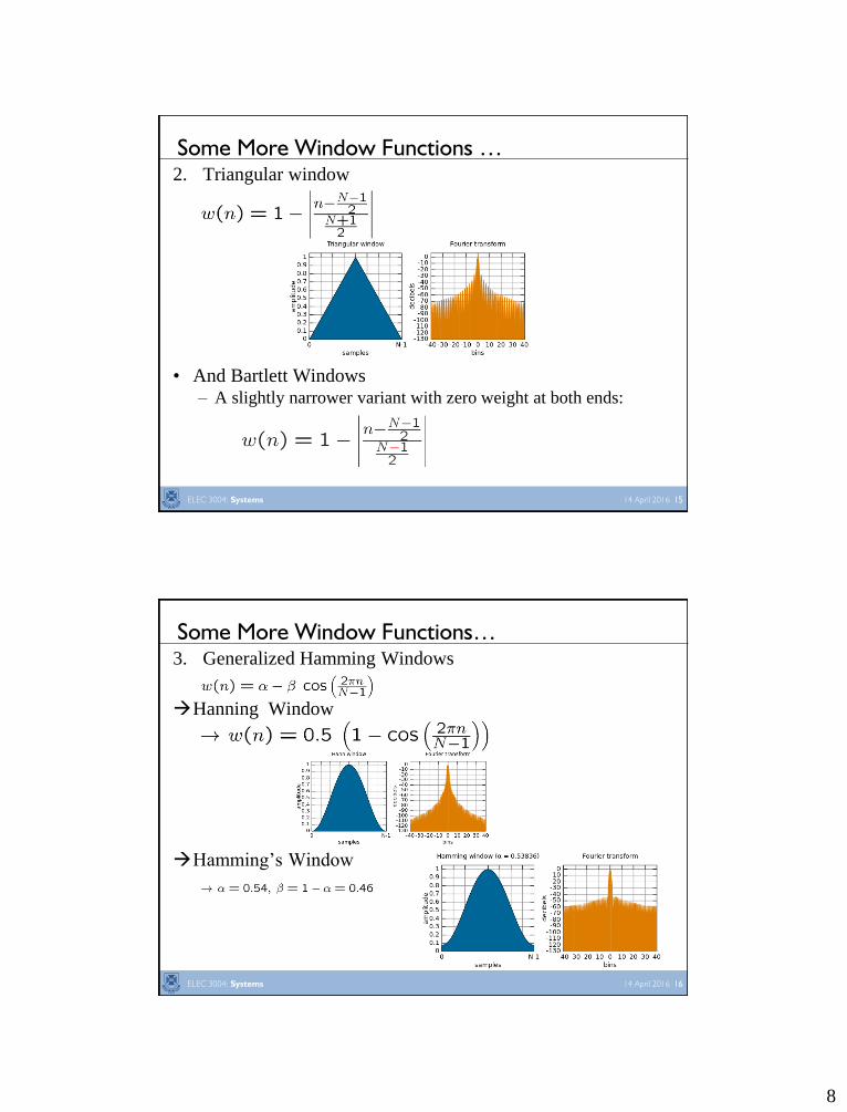
2. Triangular window

• And Bartlett Windows – A slightly narrower variant with zero weight at both ends:

Some More Window Functions …

14 April 2016 ELEC 3004: Systems 15

3. Generalized Hamming Windows

Hanning Window

Hamming’s Window

Some More Window Functions…

14 April 2016 ELEC 3004: Systems 16

9

4. Blackman–Harris Windows – A generalization of the Hamming family,

– Adds more shifted functions for less side-lobe levels

Some More Window Functions…

14 April 2016 ELEC 3004: Systems 17

5. Kaiser window – A DPSS (discrete prolate spheroidal sequence)

– Maximize the energy concentration in the main lobe

– Where: I0 is the zero-th order modified Bessel function of the

first kind, and usually α = 3.

Some More Window Functions…

14 April 2016 ELEC 3004: Systems 18

10

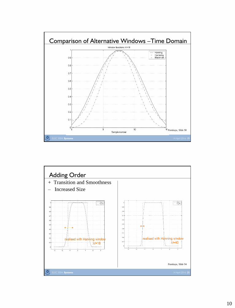
Comparison of Alternative Windows –Time Domain

Punskaya, Slide 90

14 April 2016 ELEC 3004: Systems 19

+ Transition and Smoothness

– Increased Size

Adding Order

Punskaya, Slide 94

14 April 2016 ELEC 3004: Systems 20

11

Comparison of Alternative Windows Frequency Domain

Punskaya, Slide 91

14 April 2016 ELEC 3004: Systems 21

Summary Characteristics of Common Window Functions

Lathi, Table 7.3

Punskaya, Slide 92

14 April 2016 ELEC 3004: Systems 22

12

FIR: Rectangular & Hanning Windows

• Rectangular

• Hanning

Hanning: Less ripples, but wider transition band Punskaya, Slide 93

14 April 2016 ELEC 3004: Systems 23

Punskaya, Slide 96

• Equal transition bandwidth on both sides

of the ideal cutoff frequency

Windowed FIR Property 1: Equal transition bandwidth

14 April 2016 ELEC 3004: Systems 24

13

Punskaya, Slide 96

• Peak approximation error in the passband (1+δ 1-δ)

is equal to that in the stopband (δ -δ)

Windowed FIR Property 2: Peak Errors same in Passband & Stopband

14 April 2016 ELEC 3004: Systems 25

Punskaya, Slide 99

• The distance between approximation error peaks is

approximately equal to the width of the mainlobe Δwm

Windowed FIR Property 3: Mainlobe Width

14 April 2016 ELEC 3004: Systems 26

14

Punskaya, Slide 96

• The width of the mainlobe is wider than

the transition bandwidth

Windowed FIR Property 4: Mainlobe Width [2]

14 April 2016 ELEC 3004: Systems 27

Punskaya, Slide 96

• peak approximation error is determined by

the window shape, independent of the filter order

Windowed FIR Property 5: Peak Δδ is determined by the window shape

14 April 2016 ELEC 3004: Systems 28

15

Where:

• ωc: cutoff frequency

• δ: maximum

passband ripple

• Δω: transition bandwidth

• Δωm: width of the

window mainlobe

Window Design Method Design Terminology

Punskaya, Slide 96

14 April 2016 ELEC 3004: Systems 29

ωs and ωp: Corner Frequencies

Passband / stopband ripples are often expressed in dB:

• passband ripple = 20 log10 (1+δp ) dB

• peak-to-peak passband ripple ≅ 20 log10 (1+2δp) dB

• minimum stopband attenuation = -20 log10 (δs) dB

Passband / stopband ripples

14 April 2016 ELEC 3004: Systems 30

16

ωs and ωp: Corner Frequencies

Passband / stopband ripples are often expressed in dB:

• passband ripple = 20 log10 (1+δp ) dB = 20 log10 (δp ) dB

• peak-to-peak passband ripple ≅ 20 log10 (1+2δp) dB

≅ 20 log10 (2δp) dB

• minimum stopband attenuation = -20 log10 (δs) dB

=20 log10 (δs) dB

Passband / stopband ripples

14 April 2016 ELEC 3004: Systems 31

1. Select a suitable window function

2. Specify an ideal response Hd(ω)

3. Compute the coefficients of the ideal filter hd(n)

4. Multiply the ideal coefficients by the window function to

give the filter coefficients

5. Evaluate the frequency response of the resulting filter and

iterate if necessary (e.g. by increasing M if the specified

constraints have not been satisfied).

Summary of Design Procedure

Punskaya, Slide 105

14 April 2016 ELEC 3004: Systems 32

17

• Design a type I low-pass filter with: – ωp =0.2π

– ωs =0.3π

– δ =0.01

Windowed Filter Design Example

14 April 2016 ELEC 3004: Systems 33

• LP with: ωp =0.2π, ωs =0.3π, δ =0.01

• δ =0.01: The required peak error spec: -20log10 (δ) = –40 dB

• Main-lobe width:

ωs-ωp=0.3π-0.2π =0.1π 0.1π = 8π / M

Filter length M ≥ 80 & Filter order N ≥ 79

• BUT, Type-I filters have even order so N = 80

Windowed Filter Design Example: Step 1: Select a suitable Window Function

Hanning Window

14 April 2016 ELEC 3004: Systems 34

18

• From Property 1 (Midpoint rule)

∴ An ideal response will be:

Windowed Filter Design Example: Step 2: Specify the Ideal Response

ωc = (ωs + ωp)/2 = (0.2π+0.3π)/2 = 0.25π

14 April 2016 ELEC 3004: Systems 35

• The ideal filter coefficients hd are given by the

Inverse Discrete time Fourier transform of Hd(ω)

+ Delayed impulse response (to make it causal)

• Coefficients of the ideal filter (via equation or IFFT):

Windowed Filter Design Example: Step 3: Compute the coefficients of the ideal filter

14 April 2016 ELEC 3004: Systems 36

19

• Multiply by a Hamming window function for the passband:

Windowed Filter Design Example: Step 4: Multiply to obtain the filter coefficients

14 April 2016 ELEC 3004: Systems 37

• The frequency response is computed as the DFT

of the filter coefficient vector

• If the resulting filter does not meet the specifications, then: – Adjust the ideal filter frequency response

(for example, move the band edge) and repeat (step 2)

– Adjust the filter length and repeat (step 4)

– change the window (& filter length) (step 4)

• And/Or consult with Matlab: – FIR1 and FIR2

– B=FIR2(N,F,M): Designs a Nth order FIR digital filter with

Windowed Filter Design Example: Step 5: Evaluate the Frequency Response and Iterate

14 April 2016 ELEC 3004: Systems 38

20

• FIR1 and FIR2 – B=FIR2(N,F,M): Designs a Nth order FIR digital filter

– F and M specify frequency and magnitude breakpoints for the

filter such that plot(N,F,M) shows a plot of desired frequency

– Frequencies F must be in increasing order between 0 and Fs/2,

with Fs corresponding to the sample rate.

– B is the vector of length N+1,

it is real, has linear phase and symmetric coefficients

– Default window is Hamming – others can be specified

Windowed Filter Design Example: Consulting Matlab:

14 April 2016 ELEC 3004: Systems 39

• FIR Filters are digital (can not be implemented in analog) and

exploit the difference and delay operators

• A window based design builds on the notion of a truncation of

the “ideal” box-car or rectangular low-pass filter in the

Frequency domain (which is a sinc function in the time domain)

• Other Design Methods exist: – Least-Square Design

– Equiripple Design

– Remez method

– The Parks-McClellan Remez algorithm

– Optimisation routines …

In Conclusion

14 April 2016 ELEC 3004: Systems 40

21

• Digital Filters

• Review: – Chapter 12 of Lathi

• Ponder?

Next Time…

14 April 2016 ELEC 3004: Systems 41