6. Electromagnetic Radiation

We’ve seen that Maxwell’s equations allow for wave solutions. This is light. Or, more

generally, electromagnetic radiation. But how do you generate these waves from a

collection of electric charges? In other words, how do you make light?

We know that a stationary electric charge produce a stationary electric field. If we

boost this charge so it moves at a constant speed, it produces a stationary magnetic

field. In this section, we will see that propagating electromagnetic waves are created

by accelerating charges.

6.1 Retarded Potentials

We start by simply solving the Maxwell equations for a given current distribution

Jµ = (c,J). We did this in Section 2 and Section 3 for situations where both charges

and currents are independent of time. Here we’re going to solve the Maxwell equations

in full generality where the charges and currents are time dependent.

We know that we can solve half of Maxwell’s equations by introducing the gauge

potential Aµ

= (/c,A) and writing Fµ

= @µ

A

@

Aµ

. Then the remaining

equations become

@

F µ = µ0

Jµ ) Aµ @µ(@

A) = µ0

Jµ (6.1)

where is the wave operator: = @µ

@µ = (1/c2)@2/@t2 r2.

This equation is invariant under gauge transformations

Aµ ! Aµ + @µ (6.2)

Any two gauge potentials related by the transformation (6.2) are considered physically

equivalent. We will use this symmetry to help us solve (6.1). To do this we make a

gauge choice:

Claim: We can use the gauge symmetry (6.2) to choose Aµ to satisfy

@µ

Aµ = 0 (6.3)

This is known as Lorentz Gauge. It was actually discovered by a guy named Lorenz who

had the misfortune to discover a gauge choice that is Lorentz invariant: all observers

will agree on the gauge condition (6.3).

– 118 –

Proof: Suppose you are handed a gauge potential Aµ

which doesn’t obey (6.3) but,

instead, satisfies @µ

Aµ = f for some function f . Then do a gauge transformation of the

form (6.2). Your new gauge potential will obey @µ

Aµ + = f . This means that if

you can find a gauge transformation which satisfies = f then your new gauge

potential will be in Lorentz gauge. Such a can always be found. This follows from

general facts about di↵erential equations. (Note that this proof is essentially the same

as we used in Section 3.2.2 when proving that we could always choose Coulomb gauge

r ·A = 0).

If we are in Lorentz gauge then the Maxwell equations (6.1) become particularly

simple; they reduce to the sourced wave equation

Aµ =

1

c2@2

@t2r2

Aµ = µ

0

Jµ (6.4)

Our goal is to solve this equation, subject to the condition (6.3). As an aside, notice

that this is the same kind of equation as = f which we needed to solve to go

Lorentz gauge in the first place. This means that the methods we develop below will

allow us to solve figure out both how to go to Lorentz gauge, and also how to solve for

Aµ

once we’re there.

In the following, we’ll solve (6.4) in two (marginally) di↵erent ways. The first way is

quicker; the second way gives us a deeper understanding of what’s going on.

6.1.1 Green’s Function for the Helmholtz Equation

For our first method, we will Fourier transform Aµ

and Jµ

in time, but not in space.

We write

Aµ

(x, t) =

Z+1

1

d!

2A

µ

(x,!) ei!t and Jµ

(x, t) =

Z+1

1

d!

2Jµ

(x,!) ei!t

Now the Fourier components Aµ

(x,!) obey the equationr2 +

!2

c2

A

µ

= µ0

Jµ

(6.5)

This is the Helmholtz equation with source given by the current J .

When ! = 0, the Helmholtz equation reduces to the Poisson equation that we needed

in our discussion of electrostatics. We solved the Poisson equation using the method

of Green’s functions when discussing electrostatics in Section 2.2.3. Here we’ll do the

– 119 –

same for the Helmholtz equation. The Green’s function for the Helmholtz equation

obeys r2 +

!2

c2

G

!

(x;x0) = 3(x x0)

Translational and rotational invariance ensure that the solutions to this equation are of

the form G!

(x;x0) = G!

(r) with r = |x x0|. We can then write this as the ordinary

di↵erential equation,

1

r2d

dr

r2dG

!

dr

+

!2

c2G

!

= 3(r) (6.6)

We want solutions that vanish as r ! 1. However, even with this restriction, there

are still two such solutions. Away from the origin, they take the form

G!

e±i!r/c

r

We will see shortly that there is a nice physical interpretation of these two Green’s

functions. First, let’s figure out the coecient that sits in front of the Green’s function.

This is determined by the delta-function. We integrate both sides of (6.6) over a ball

of radius R. We get

4

ZR

0

dr r21

r2d

dr

r2dG

!

dr

+

!2

c2G

!

= 1

Now, taking the limit R ! 0, only the first term on the left-hand side survives. More-

over, only the first term of dG!

/dr (1/r2 ± i!/cr)e±i!r/c survives. We find that

the two Green’s functions for the Helmholtz equation are

G!

(r) = 1

4

e±i!r/c

r

Note that this agrees with the Green’s function for the Poisson equation when ! = 0.

Retarded Potentials

So which ± sign should we take? The answer depends on what we want to do with the

Green’s function. For our purposes, we’ll nearly always need G!

e+i!r/c/r. Let’s see

why. The Green’s function G!

allows us to write the Fourier components Aµ

in (6.5)

as

Aµ

(x,!) =µ0

4

Zd3x0 e

+i!|xx

0|/c

|x x0| Jµ

(x0,!)

– 120 –

which, in turn, means that the time-dependent gauge potential becomes

Aµ

(x, t) =µ0

4

Zd!

2

Zd3x0 e

i!(t|xx

0|/c)

|x x0| Jµ

(x0)

But now the integral over ! is just the inverse Fourier transform. With one di↵erence:

what was the time variable t has become the retarted time, tret

, with

ctret

= ct |x x0|

We have our final result,

Aµ

(x, t) =µ0

4

Zd3x0 Jµ(x

0, tret

)

|x x0| (6.7)

This is called the retarded potential. To determine the contribution at point x and time

t, we integrate the current over all of space, weighted with the Green’s function factor

1/|x x0| which captures the fact that points further away contribute more weakly.

After all this work, we’ve arrived at something rather nice. The general form of the

answer is very similar to the result for electrostatic potential and magnetostatic vector

potential that we derived in Sections 2 and 3. Recall that when the charge density and

current were independent of time, we found

(x) =1

40

Zd3x0 (x0)

|x x0| and A(x) =µ0

4

Zd3x0 J(x0)

|x x0|But when the charge density and current do depend on time, we see from (6.7) that

something new happens: the gauge field at point x and time t depends on the current

configuration at point x0 and the earlier time tret

= t |xx0|/c. This, of course, is dueto causality. The di↵erence t t

ret

is just the time it took the signal to propagate from

x0 to x, travelling at the speed of light. Of course, we know that Maxwell’s equations

are consistent with relativity so something like this had to happen; we couldn’t have

signals travelling instantaneously. Nonetheless, it’s pleasing to see how this drops out

of our Green’s functionology.

Finally, we can see what would happen were we to choose the other Green’s function,

G!

ei!r/c/r. Following through the steps above, we see that the retarded time tret

is replaced by the advanced time tadv

= t + |x x0|/c. Such a solution would mean

that the gauge field depends on what the current is doing in the future, rather than in

the past. These solutions are typically thrown out as being unphysical. We’ll have (a

little) more to say about them at the end of the next section.

– 121 –

6.1.2 Green’s Function for the Wave Equation

The expression for the retarded potential (6.7) is important. In this section, we provide

a slightly di↵erent derivation. This will give us more insight into the origin of the

retarded and advanced solutions. Moreover, the techniques below will also be useful in

later courses3.

We started our previous derivation by Fourier transforming only the time coordinate,

to change the wave equation into the Helmholtz equation. Here we’ll treat time and

space on more equal footing and solve the wave equation directly. We again make use

of Green’s functions. The Green’s function for the wave equation obeysr2 1

c2@2

@t2

G(x, t;x0, t0) = 3(x x0)(t t0) (6.8)

Translational invariance in space and time means that the Green’s function takes the

form G(x, t;x0, t) = G(xx0, tt0). To determine this function G(r, t), with r = xx0,

we Fourier transform both space and time coordinates,

G(x, t) =

Zdw d3k

(2)4G(k,!) ei(k·r!t) (6.9)

Choosing x0 = 0 and t0 = 0, the wave equation (6.8) then becomesr2 1

c2@2

@t2

G(r, t) =

Zdw d3k

(2)4G(!,k)

r2 1

c2@2

@t2

ei(k·r!t)

=

Zdw d3k

(2)4G(k,!)

k2 +

!2

c2

ei(k·r!t)

= 3(r)(t) =

Zdw d3k

(2)4ei(k·r!t)

Equating the terms inside the integral, we see that the Fourier transform of the Green’s

function takes the simple form

G(k,!) = 1

k2 !2/c2

But notice that this diverges when !2 = c2k2. This pole results in an ambiguity in the

Green’s function in real space which, from (6.9), is given by

G(r, t) = Z

dw d3k

(2)41

k2 !2/c2ei(k·r!t)

3A very similar discussion can be found in the lecture notes on Quantum Field Theory.

– 122 –

We need some way of dealing with that pole in the integral. To see what’s going on,

it’s useful to change to polar coordinates for the momentum integrals over k. This will

allow us to deal with that eik·r factor. The best way to do this is to think of fixing r

and then choosing the kz

axis to point along x. We then write k · r = kr cos , and the

Green’s function becomes

G(r, t) = 1

(2)4

Z2

0

d

Z

0

d sin

Z 1

0

dk k2

Z+1

1d!

1

k2 !2/c2ei(kr cos !t)

Now the d integral is trivial, while the d integral isZ

0

d sin eikr cos = 1

ikr

Z

0

d

d

deikr cos

= 1

ikr

eikr e+ikr

= 2

sin kr

kr

After performing these angular integrals, the real space Green’s function becomes

G(r, t) =1

43

Z 1

0

dk c2k2

sin kr

kr

Z+1

1d!

ei!t

(! ck)(! + ck)

Now we have to face up to those poles. We’ll work by fixing k and doing the ! integral

first. (Afterwards, we’ll then have to do the k integral). It’s clear that we run into two

poles at ! = ±ck when we do the ! integral and we need a prescription for dealing

with these. To do this, we need to pick a contour C in the complex ! plane which

runs along the real axis but skips around the poles. There are di↵erent choices for C.

Each of them provides a Green’s function which obeys (6.8) but, as we will now see,

these Green’s functions are di↵erent. What’s more, this di↵erence has a nice physical

interpretation.

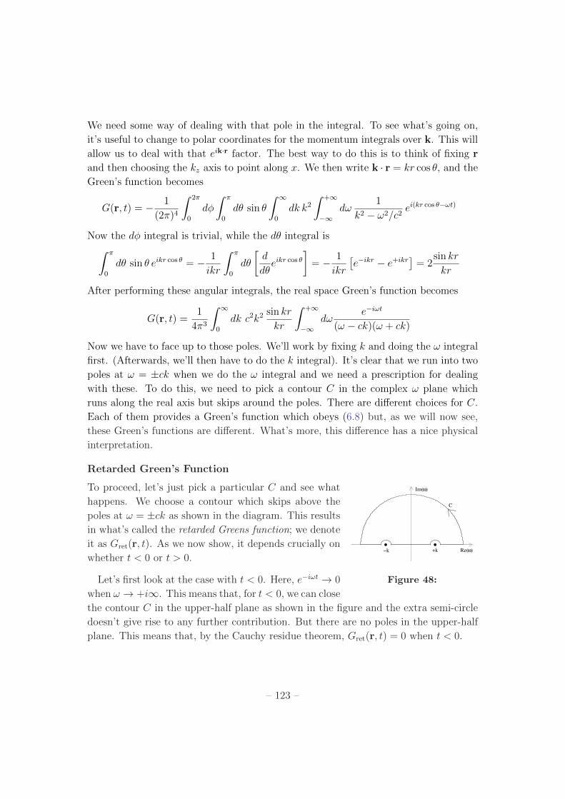
Retarded Green’s Function

To proceed, let’s just pick a particular C and see what

Re( )ω

Im( )ω

C

−k +k

Figure 48:

happens. We choose a contour which skips above the

poles at ! = ±ck as shown in the diagram. This results

in what’s called the retarded Greens function; we denote

it as Gret

(r, t). As we now show, it depends crucially on

whether t < 0 or t > 0.

Let’s first look at the case with t < 0. Here, ei!t ! 0

when ! ! +i1. This means that, for t < 0, we can close

the contour C in the upper-half plane as shown in the figure and the extra semi-circle

doesn’t give rise to any further contribution. But there are no poles in the upper-half

plane. This means that, by the Cauchy residue theorem, Gret

(r, t) = 0 when t < 0.

– 123 –

In contrast, when t > 0 we have ei!t ! 0 when ! ! i1, which means that we

get to close the contour in the lower-half plane. Now we do pick up contributions to

the integral from the two poles at ! = ±ck. This time the Cauchy residue theorem

gives

ZC

d!ei!t

(! ck)(! + ck)= 2i

eickt

2ck e+ickt

2ck

= 2

cksin ckt (t > 0)

So, for t > 0, the Green’s function becomes

Gret

(r, t) = 1

22

1

r

Z 1

0

dk c sin kr sin ckt

=1

42

1

r

Z 1

1dk

c

4(eikr eikr)(eickt eickt)

=1

42

1

r

Z 1

1dk

c

4(eik(r+ct) + eik(r+ct) eik(rct) eik(rct))

Each of these final integrals is a delta-function of the form (r ± ct). But, obviously,

r > 0 while this form of the Green’s function is only valid for t > 0. So the (r + ct)

terms don’t contribute and we’re left with

Gret

(x, t) = 1

4

c

r(r ct) t > 0

We can absorb the factor of c into the delta-function. (Recall that (x/a) = |a|(x) forany constant a). So we finally get the answer for the retarded Green’s function

Gret

(r, t) =

8<: 0 t < 0

1

4r(t

ret

) t > 0

where tret

is the retarded time that we met earlier,

tret

= t r

c

The delta-function ensures that the Green’s function is only non-vanishing on the light-

cone emanating from the origin.

– 124 –

Finally, with the retarded Green’s function in hand, we can construct what we really

want: solutions to the wave equation (6.4). These solutions are given by

Aµ

(x, t) = µ0

Zd3x0dt0 G

ret

(x, t;x0, t0) Jµ

(x0, t0) (6.10)

=µ0

4

Zd3x0dt0

(tret

)

|x x0|Jµ(x0, t0)

=µ0

4

Zd3x0 Jµ(x

0, tret

)

|x x0|Happily, we find the same expression for the retarded potential that we derived previ-

ously in (6.7).

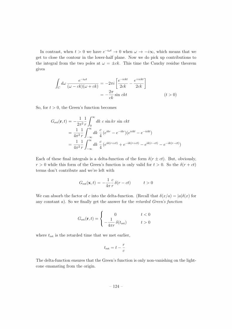
Advanced Green’s Function

Let us briefly look at other Green’s functions. We canRe( )ω

Im( )ω

C

+k−k

Figure 49:

pick the contour C in the complex !-plane to skip below

the two poles on the real axis. This results in what’s

called the advanced Green’s function. Now, when t >

0, we complete the contour in the lower-half plane, as

shown in the figure, where the lack of poles means that

the advanced Green’s function vanishes. Meanwhile, for

t < 0, we complete the contour in the upper-half plane

and get

Gadv

(r, t) =

8<: 1

4r(t

adv

) t < 0

0 t > 0

where

tadv

= t+r

c

The resulting solution gives a solution known as the advanced potential,

Aµ

(x, t) =µ0

4

Zd3x0 Jµ(x

0, tadv

)

|x x0|It’s hard to think of this solution as anything other than unphysical. Taken at face

value, the e↵ect of the current and charges now propagates backwards in time to de-

termine the gauge potential Aµ

. The sensible thing is clearly to throw these solutions

away.

– 125 –

However, it’s worth pointing out that the choice of the retarded propagator Gret

rather than the advanced propagator Gadv

is an extra ingredient that we should add to

the theory of electromagnetism. The Maxwell equations themselves are time symmetric;

the choice of which solutions are physical is not.

There is some interesting history attached to this. A number of physicists have felt

uncomfortable at imposing this time asymmetry only at the level of solutions, and

attempted to rescue the advanced propagator in some way. The most well-known of

these is the Feynman-Wheeler absorber theory, which uses a time symmetric propaga-

tor, with the time asymmetry arising from boundary conditions. However, I think it’s

fair to say that these ideas have not resulted in any deeper understanding of how time

emerges in physics.

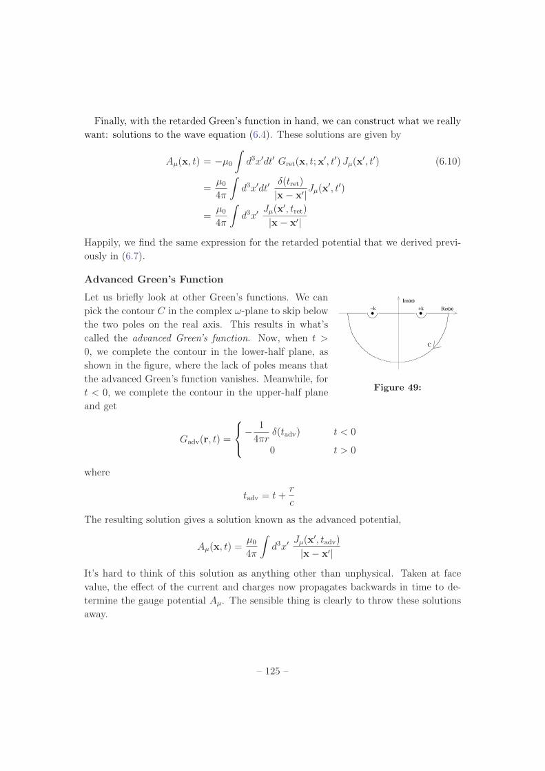
Finally, there is yet another propagator that we canRe( )ω

Im( )ω

C −k

+k

Figure 50:

use. This comes from picking a contour C that skips

under the first pole and over the second. It is known as

the Feynman propagator and plays an important role in

quantum field theory.

6.1.3 Checking Lorentz Gauge

There is a loose end hanging over from our previous discussion. We have derived the

general solution to the wave equation (6.4) for Aµ

.This is given by the retarded potential

Aµ

(x, t) =µ0

4

Zd3x0 Jµ(x

0, tret

)

|x x0| (6.11)

But the wave equation is only equivalent to the Maxwell equations if it obeys the

Lorentz gauge fixing condition, @µ

Aµ = 0. We still need to check that this holds. In

fact, this follows from the conservation of the current: @µ

Jµ = 0. To show this, it’s

actually simplest to return to a slightly earlier form of this expression (6.10)

Aµ

(x, t) = µ0

Zd3x0dt0 G

ret

(x, t;x0, t0) Jµ

(x0, t0)

The advantage of this is that both time and space remain on an equal footing. We have

@µ

Aµ(x, t) = µ0

Zd3x0dt0 @

µ

Gret

(x, t;x0, t0) Jµ(x0, t0)

But now we use the fact that Gret

(x, t;x0, t0) depends on xx0 and t t0 to change the

derivative @µ

acting on x into a derivative @0µ

acting on x0. We pick up a minus sign for

– 126 –

our troubles. We then integrate by parts to find,

@µ

Aµ(x, t) = +µ0

Zd3x0dt0 @0

µ

Gret

(x, t;x0, t0) Jµ(x0, t0)

= µ0

Zd3x0dt0 G

ret

(x, t;x0, t0) @0µ

Jµ(x0, t0)

= 0

as required. If you prefer, you can also run through the same basic steps with the form

of the solution (6.11). You have to be a little careful because tret

now also depends on

x and x0 so you get extra terms at various stages when you di↵erentiate. But it all

drops out in the wash and you again find that Lorentz gauge is satisfied courtesy of

current conservation.

6.2 Dipole Radiation

Let’s now use our retarded potential do understand something new. This is the set-

up: there’s some localised region V in which there is a time-dependent distribution of

charges and currents. But we’re a long way from this region. We want to know what

the resulting electromagnetic field looks like.

Our basic formula is the retarded potential,

Aµ

(x, t) =µ0

4

ZV

d3x0 Jµ(x0, t

ret

)

|x x0| (6.12)

The current Jµ(x0, t) is non-zero only for x0 2 V . We denote the size of the region V

as d and we’re interested in what’s happening at a point x which is a distance r = |x|away. (A word of warning: in this section we’re using r = |x| which di↵ers from our

notation in Section 6.1 where we used r = |x x0|). If |x x0| a for all x0 2 V then

we can approximate |xx0| |x| = r. In fact, we will keep the leading order correction

to this which we get by Taylor expansion. (This is the same Taylor expansion that we

needed when deriving the multipole expansion for electrostatics in Section 2.2.3). We

have

|x x0| = r x · x0

r+ . . .

) 1

|x x0| =1

r+

x · x0

r3+ . . . (6.13)

There is a new ingredient compared to the electrostatic case: we have a factor of |xx0|that sits inside t

ret

= t |x x0|/c as well, so that

Jµ

(x0, tret

) = Jµ

(x0, t r/c+ x · x0/rc+ . . .)

– 127 –

Now we’d like to further expand out this argument. But, to do that, we need to know

something about what the current is doing. We will assume hat the motion of the

charges and current are non-relativistic so that the current doesn’t change very much

over the time d/c that it takes light to cross the region V . For example, if the

current varies with characteristic frequency ! (so that J ei!t), then this requirement

becomes d/c 1/!. Then we can further Taylor expand the current to write

Jµ

(x0, tret

) = Jµ

(x0, t r/c) + Jµ

(x0, t r/c)x · x0

rc+ . . . (6.14)

We start by looking at the leading order terms in both these Taylor expansions.

6.2.1 Electric Dipole Radiation

At leading order in d/r, the retarded potential becomes simply

Aµ

(x, t) µ0

4r

ZV

d3x0 Jµ

(x0, t r/c)

This is known as the electric dipole approximation. (We’ll see why very shortly). We

want to use this to compute the electric and magnetic fields far from the localised source.

It turns out to be simplest to first compute the magnetic field using the 3-vector form

of the above equation,

A(x, t) µ0

4r

ZV

d3x0 J(x0, t r/c)

We can manipulate the integral of the current using the conservation formula +r ·J = 0. (The argument is basically a repeat of the kind of arguments we used in the

magnetostatics section 3.3.2). We do this by first noting the identity

@j

(Jj

xi

) = (@j

Jj

) xi

+ Ji

= xi

+ Ji

We integrate this over all of space and discard the total derivative to findZd3x0 J(x0) =

d

dt

Zd3x0 (x0)x0 = p

where we recognise p as the electric dipole moment of the configuration. We learn that

the vector potential is determined by the change of the electric dipole moment,

A(x, t) µ0

4rp(t r/c)

This, of course, is where the electric dipole approximation gets its name.

– 128 –

We now use this to compute the magnetic field B = rA. There are two contri-

butions: one when r acts on the 1/r term, and another when r acts on the r in the

argument of p. These give, respectively,

B µ0

4r2x p(t r/c) µ

0

4rcx p(t r/c)

where we’ve used the fact that rr = x. Which of these two terms is bigger? As we

get further from the source, we would expect that the second, 1/r, term dominates

over the first, 1/r2 term. We can make this more precise. Suppose that the source is

oscillating at some frequency !, so that p !p. We expect that it will make waves

at the characteristic wavelength = c/!. Then, as long we’re at distances r , the

second term dominates and we have

B(t,x) µ0

4rcx p(t r/c) (6.15)

The region r is called the far-field zone or, sometimes, the radiation zone. We’ve

now made two successive approximations, valid if we have a hierarchy of scales in our

problem: r d.

To get the corresponding electric field, it’s actually simpler to use the Maxwell equa-

tion E = c2rB. Again, if we care only about large distances, r , the curl of B

is dominated by r acting on the argument of p. We get

rB µ0

4rc2x (x ...

p(t r/c))

) E µ0

4rx (x p(t r/c)) (6.16)

Notice that the electric and magnetic field are related in the same way that we saw for

plane waves, namely

E = c xB

although, now, this only holds when we’re suitably far from the source, r . What’s

happening here is that oscillating dipole is emitting spherical waves. At radius r

these can be thought of as essentially planar.

Notice, also, that the electric field is dropping o↵ slowly as 1/r. This, of course, is

even slower than the usual Coulomb force fall-o↵.

– 129 –

6.2.2 Power Radiated: Larmor Formula

We can look at the power radiated away by the source. This is computed by the

Poynting vector which we first met in Section 4.4. It is given by

S =1

µ0

EB =c

µ0

|B|2x =µ0

162r2c|x p|2 x

The fact that S lies in the direction xmeans that the power is emitted radially. The fact

that it drops o↵ as 1/r2 follows from the conservation of energy. It means that the total

energy flux, computed by integrating S over a large surface, is constant, independent

of r.

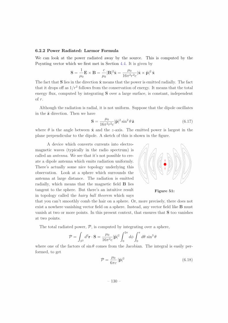
Although the radiation is radial, it is not uniform. Suppose that the dipole oscillates

in the z direction. Then we have

S =µ0

162r2c|p|2 sin2 z (6.17)

where is the angle between x and the z-axis. The emitted power is largest in the

plane perpendicular to the dipole. A sketch of this is shown in the figure.

A device which converts currents into electro-

Figure 51:

magnetic waves (typically in the radio spectrum) is

called an antenna. We see that it’s not possible to cre-

ate a dipole antenna which emits radiation uniformly.

There’s actually some nice topology underlying this

observation. Look at a sphere which surrounds the

antenna at large distance. The radiation is emitted

radially, which means that the magnetic field B lies

tangent to the sphere. But there’s an intuitive result

in topology called the hairy ball theorem which says

that you can’t smoothly comb the hair on a sphere. Or, more precisely, there does not

exist a nowhere vanishing vector field on a sphere. Instead, any vector field like B must

vanish at two or more points. In this present context, that ensures that S too vanishes

at two points.

The total radiated power, P , is computed by integrating over a sphere,

P =

ZS

2

d2r · S =µ0

162c|p|2

Z2

0

d

Z

0

d sin3

where one of the factors of sin comes from the Jacobian. The integral is easily per-

formed, to get

P =µ0

6c|p|2 (6.18)

– 130 –

Finally, the dipole term p is still time dependent. It’s common practice to compute the

time averaged power. The most common example is when the dipole oscillates with

frequency !, so that |p|2 cos2(!t). (Recall that we’re only allowed to work with

complex expressions when we have linear equations). Then, integrating over a period,

T = 2/!, just gives an extra factor of 1/2.

Let’s look at a simple example. Take a particle of charge Q, oscillating in the z

direction with frequency ! and amplitude d. Then we have p = pzei!t with the dipole

moment p = Qd. Similarly, p = !2pzei!t. The end result for the time averaged power

P is

P =µ0

p2!4

12c(6.19)

This is the Larmor formula for the time-averaged power radiated by an oscillating

charge. The formula is often described in terms of the acceleration, a = d!2. Then it

reads

P =Q2a2

120

c3(6.20)

where we’ve also swapped the µ0

in the numerator for 0

c2 in the denominator.

6.2.3 An Application: Instability of Classical Matter

The popular picture of an atom consists of a bunch of electrons

Figure 52: This is

not what an atom

looks like.

orbiting a nucleus, like planets around a star. But this isn’t what

an atom looks like. Let’s see why.

We’ll consider a Hydrogen atom, with an electron orbiting around

a proton, fixed at the origin. (The two really orbit each other

around their common centre of mass, but the mass of the electron

is me

9 1031 Kg, while the mass of the proton is about 1800

bigger, so this is a good approximation). The equation of motion

for the electron is

me

r = e2

40

r

r2

The dipole moment of the atom is p = er so the equation of motion tells us p. Plugging

this into (6.18), we can get an expression for the amount of energy emitted by the

electron,

P =µ0

6c

e3

40

me

r2

2

– 131 –

As the electron emits radiation, it loses energy and must, therefore, spiral towards the

nucleus. We know from classical mechanics that the energy of the orbit depends on its

eccentricity. For simplicity, let’s assume that the orbit is circular with energy

E = e2

40

1

2r

Then we can equate the change in energy with the emitted power to get

E =e2

80

r2r = P = µ

0

6c

e3

40

me

r2

2

which gives us an equation that tells us how the radius of the orbit changes,

r = µ0

e4

122c0

m2

e

r2

Suppose that we start at some time, t = 0, with a classical orbit with radius r0

. Then

we can calculate how long it takes for the electron to spiral down to the origin at r = 0.

It is

T =

ZT

0

dt =

Z0

r0

1

rdr =

42c0

m2

e

r30

µ0

e4

Now let’s plug in some small numbers. We can take the size of the atom to be r0

5 1011m. (This is roughly the Bohr radius that can be derived theoretically using

quantum mechanics). Then we find that the lifetime of the hydrogen atom is

T 1011 s

That’s a little on the small size. The Universe is 14 billion years old and hydrogen

atoms seem in no danger of decaying.

Of course, what we’re learning here is something dramatic: the whole framework of

classical physics breaks down when we look at the atomic scale and has to be replaced

with quantum mechanics. And, although we talk about electron orbits in quantum

mechanics, they are very di↵erent objects than the classical orbits drawn in the picture.

In particular, an electron in the ground state of the hydrogen atom emits no radiation.

(Electrons in higher states do emit radiation with some probability, ultimately decaying

down to the ground state).

6.2.4 Magnetic Dipole and Electric Quadrupole Radiation

The electric dipole approximation to radiation is sucient for most applications. Ob-

vious exceptions are when the dipole p vanishes or, for some reason, doesn’t change in

time. For completeness, we describe here the leading order corrections to the electric

dipole approximations.

– 132 –

The Taylor expansion of the retarded potential was given in (6.13) and (6.14).

Putting them together, we get

Aµ

(x, t) =µ0

4

ZA

d3x0 Jµ(x0, t

ret

)

|x x0|=

µ0

4r

ZA

d3x0Jµ

(x0, t r/c) + Jµ

(x0, t r/c)x · x0

rc

1 +

x · x0

r2

+ . . .

The first term is the electric dipole approximation that we discussed in above. We will

refer to this as AED

µ

. Corrections to this arise as two Taylor series. Ultimately we will

only be interested in the far-field region. At far enough distance, the terms in the first

bracket will always dominate the terms in the second bracket, which are suppressed by

1/r. We therefore have

Aµ

(x, t) AED

µ

(x, t) +µ0

4r2c

ZA

d3x0 (x · x0)Jµ

(x0, t r/c)

As in the electric dipole case, it’s simplest if we focus on the vector potential

A(x, t) AED(x, t) +µ0

4r2c

Zd3x0 (x · x0) J(x0, t r/c) (6.21)

The integral involves the kind of expression that we met first when we discussed mag-

netic dipoles in Section 3.3.2. We use the slightly odd expression,

@j

(Jj

xi

xk

) = (@j

Jj

)xi

xk

+ Ji

xk

+ Jk

xi

= xi

xk

+ Ji

xk

+ Jk

xi

Because J in (6.21) is a function of x0, we apply this identity to the Ji

x0j

terms in the

expression. We drop the boundary term at infinity, remembering that we’re actually

dealing with J rather than J , write the integral above asZd3x0 x

j

x0j

Ji

=xj

2

Zd3x0 (x0

j

Ji

x0i

Jj

+ x0i

x0j

)

Then, using the appropriate vector product identity, we haveZd3x0 (x · x0)J =

1

2x

Zd3x0 J x0 +

1

2

Zd3x0 (x · x0)x0

Using this, we may write (6.21) as

A(x, t) AED(x, t) +AMD(x, t) +AEQ(x, t)

where AMD is the magnetic dipole contribution and is given by

AMD(x, t) = µ0

8r2cx

Zd3x0 x0 J(x0, t r/c) (6.22)

– 133 –

and AEQ is the electric quadrupole contribution and is given by

AEQ(x, t) =µ0

8r2c

Zd3x0 (x · x0)x0 (x0, t r/c) (6.23)

The names we have given to each of these contributions will become clearer as we look

at their properties in more detail.

Magnetic Dipole Radiation

Recall that, for a general current distribution, the magnetic dipole m is defined by

m =1

2

Zd3x0 x0 J(x0)

The magnetic dipole contribution to radiation (6.22) can then be written as

AMD(x, t) = µ0

4rcx m(t r/c)

This means that varying loops of current will also emit radiation. Once again, the

leading order contribution to the magnetic field, B = rA, arises when the curl hits

the argument of m. We have

BMD(x, t) µ0

4rc2x (x m(t r/c))

Using the Maxwell equation EMD = c2rBMD to compute the electric field, we have

EMD(x, t) µ0

4rcx m(t r/c)

The end result is very similar to the expression for B and E that we saw in (6.15) and

(6.16) for the electric dipole radiation. This means that the radiated power has the

same angular form, with the Poynting vector now given by

SMD =µ0

162r2c3|m|2 sin2 z (6.24)

Integrating over all space gives us the power emitted,

PMD =µ0

6c3|m|2 (6.25)

This takes the same form as the electric dipole result (6.18), but with the electric dipole

replaced by the magnetic dipole. Notice, however, that for non-relativistic particles, the

magnetic dipole radiation is substantially smaller than the electric dipole contribution.

For a particle of charge Q, oscillating a distance d with frequency !, we have p Qd

and m Qd2!. This means that the ratio of radiated powers is

PMD

PED

d2!2

c2 v2

c2

where v is the speed of the particle.

– 134 –

Electric Quadrupole Radiation

The electric quadrupole tensor Qij

arises as the 1/r4 term in the expansion of the

electric field for a general, static charge distribution. It is defined by

Qij

=

Zd3x0 (x0)

3x0

i

x0j

ij

x0 2This is not quite of the right form to account for the contribution to the potential

(6.23). Instead, we have

AEQ

i

(x, t) = µ0

24r2c

xj

Qij

(t r/c) + xi

Zd3x0 x02(x0, t r/c)

The second term looks like a mess, but it doesn’t do anything. This is because it’s

radial and so vanishes when we take the curl to compute the magnetic field. Neither

does it contribute to the electric field which, in our case, we will again determine from

the Maxwell equation. This means we are entitled to write

AEQ(x, t) = µ0

24r2cx · Q(t r/c)

where (x · Q)i

= xj

Qij

. Correspondingly, the magnetic and electric fields at large

distance are

BEQ(x, t) µ0

24rc2x (x · Q)

EEQ(x, t) µ0

24rc((x ·Q · x)x (x ·Q))

We may again compute the Poynting vector and radiated power. The details depend on

the exact structure of Q, but the angular dependence of the radiation is now di↵erent

from that seen in the dipole cases.

Finally, you may wonder about the cross terms between the ED, MD and EQ com-

ponents of the field strengths when computing the quadratic Poynting vector. It turns

out that, courtesy of their di↵erent spatial structures, these cross-term vanish when

computing the total integrated power.

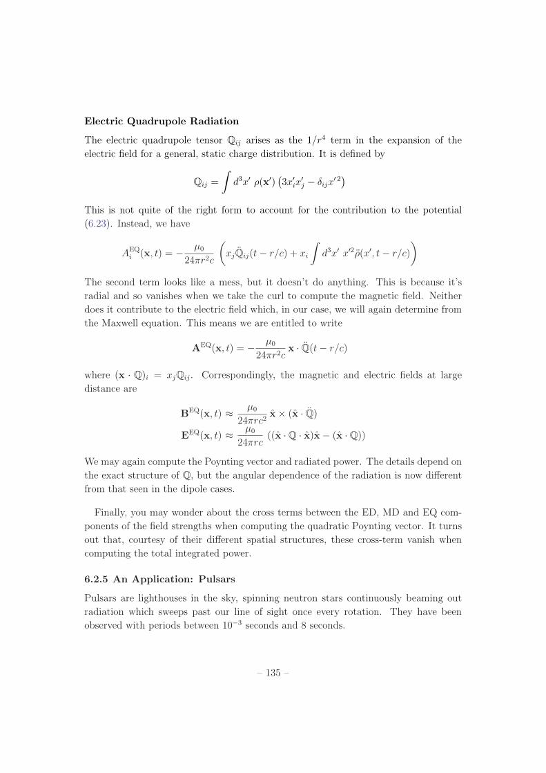
6.2.5 An Application: Pulsars

Pulsars are lighthouses in the sky, spinning neutron stars continuously beaming out

radiation which sweeps past our line of sight once every rotation. They have been

observed with periods between 103 seconds and 8 seconds.

– 135 –

Neutron stars typically carry a very large magnetic field. This arises from the parent

star which, as it collapses, reduces in size by a factor of about 105. This squeezes the

magnetic flux lines, which gets multiplied by a factor of 1010. The resulting magnetic

field is typically around 108 Tesla, but can be as high as 1011 Tesla. For comparison,

the highest magnetic field that we have succeeded in creating in a laboratory is a paltry

100 Tesla or so.

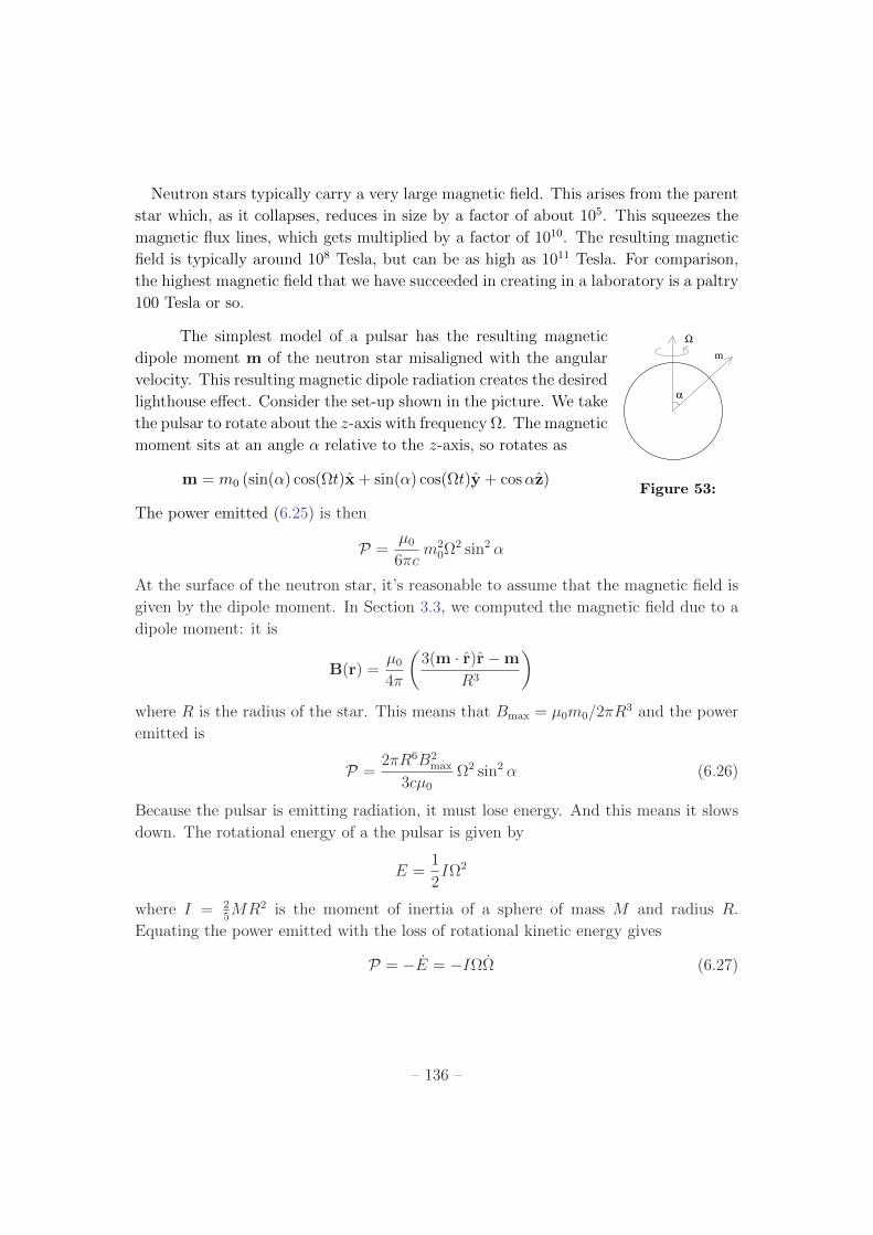
The simplest model of a pulsar has the resulting magnetic Ω

m

α

Figure 53:

dipole moment m of the neutron star misaligned with the angular

velocity. This resulting magnetic dipole radiation creates the desired

lighthouse e↵ect. Consider the set-up shown in the picture. We take

the pulsar to rotate about the z-axis with frequency . The magnetic

moment sits at an angle ↵ relative to the z-axis, so rotates as

m = m0

(sin(↵) cos(t)x+ sin(↵) cos(t)y + cos↵z)

The power emitted (6.25) is then

P =µ0

6cm2

0

2 sin2 ↵

At the surface of the neutron star, it’s reasonable to assume that the magnetic field is

given by the dipole moment. In Section 3.3, we computed the magnetic field due to a

dipole moment: it is

B(r) =µ0

4

3(m · r)rm

R3

where R is the radius of the star. This means that B

max

= µ0

m0

/2R3 and the power

emitted is

P =2R6B2

max

3cµ0

2 sin2 ↵ (6.26)

Because the pulsar is emitting radiation, it must lose energy. And this means it slows

down. The rotational energy of a the pulsar is given by

E =1

2I2

where I = 2

5

MR2 is the moment of inertia of a sphere of mass M and radius R.

Equating the power emitted with the loss of rotational kinetic energy gives

P = E = I (6.27)

– 136 –

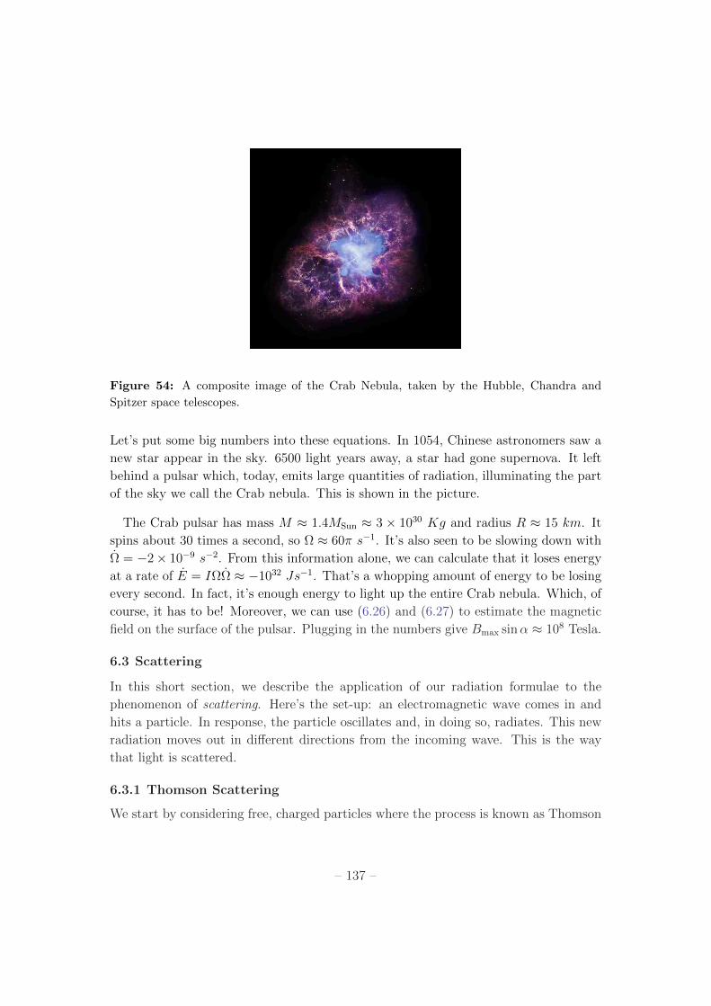
Figure 54: A composite image of the Crab Nebula, taken by the Hubble, Chandra and

Spitzer space telescopes.

Let’s put some big numbers into these equations. In 1054, Chinese astronomers saw a

new star appear in the sky. 6500 light years away, a star had gone supernova. It left

behind a pulsar which, today, emits large quantities of radiation, illuminating the part

of the sky we call the Crab nebula. This is shown in the picture.

The Crab pulsar has mass M 1.4MSun

3 1030 Kg and radius R 15 km. It

spins about 30 times a second, so 60 s1. It’s also seen to be slowing down with

= 2 109 s2. From this information alone, we can calculate that it loses energy

at a rate of E = I 1032 Js1. That’s a whopping amount of energy to be losing

every second. In fact, it’s enough energy to light up the entire Crab nebula. Which, of

course, it has to be! Moreover, we can use (6.26) and (6.27) to estimate the magnetic

field on the surface of the pulsar. Plugging in the numbers give Bmax

sin↵ 108 Tesla.

6.3 Scattering

In this short section, we describe the application of our radiation formulae to the

phenomenon of scattering. Here’s the set-up: an electromagnetic wave comes in and

hits a particle. In response, the particle oscillates and, in doing so, radiates. This new

radiation moves out in di↵erent directions from the incoming wave. This is the way

that light is scattered.

6.3.1 Thomson Scattering

We start by considering free, charged particles where the process is known as Thomson

– 137 –

scattering. The particles respond to an electric field by accelerating, as dictated by

Newton’s law

mx = qE

The incoming radiation takes the form E = E0

ei(k·r!t). To solve for the motion of the

particle, we’re going to assume that it doesn’t move very far from its central position,

which we can take to be the origin r = 0. Here, “not very far” means small compared

to the wavelength of the electric field. In this case, we can replace the electric field by

E E0

ei!t, and the particle undergoes simple harmonic motion

x(t) = qE0

m!2

sin(!t)

We should now check that the motion of the particle is indeed small compared to the

wavelength of light. The maximum distance that the particle gets is xmax

= qE0

/m!2,

so our analysis will only be valid if we satisfy

qE0

m!2

c

!) qE

0

m!c 1 (6.28)

This requirement has a happy corollary, since it also ensures that the maximum speed

of the particle vmax

= qE0

/m! c, so the particle motion is non-relativistic. This

means that we can use the dipole approximation to radiation that we developed in the

previous section. We computed the time-averaged radiated power in (6.20): it is given

by

Pradiated

=µ0

q4E2

0

12m2c

It’s often useful to compare the strength of the emitted radiation to that of the incoming

radiation. The relevant quantity to describe the incoming radiation is the time-averaged

magnitude of the Poynting vector. Recall from Section 4.4 that the Poynting vector

for a wave with wavevector k is

S =1

µ0

EB =cE2

0

µ0

k sin2(k · x !t)

Taking the time average over a single period, T = 2/!, gives us the average energy

flux of the incoming radiation,

Sincident

=cE2

0

2µ0

– 138 –

with the factor of two coming from the averaging. The ratio of the outgoing to incoming

powers is called the cross-section for scattering. It is given by

=P

radiated

Sincident

=µ2

0

q4

6m2c2

The cross-section has the dimensions of area. To highlight this, it’s useful to write it

as

=8

3r2q

(6.29)

where the length scale rq

is known as the classical radius of the particle and is given by

q2

40

rq

= mc2

This equation tells us how to think of rq

. Up to some numerical factors, it equates

the Coulomb energy of a particle in a ball of size rq

with its relativistic rest mass.

Ultimately, this is not the right way to think of the size of point particles. (The right

way involves quantum mechanics). But it is a useful concept in the classical world. For

the electron, re

2.8 1015 m.

The Thompson cross-section (6.29) is slightly smaller than the (classical) geometric

cross-section of the particle (which would be the area of the disc, 4r2q

). For us, the

most important point is that the cross-section does not depend on the frequency of

the incident light. It means that all wavelengths of light are scattered equally by

free, charged particles, at least within the regime of validity (6.28). For electrons, the

Thomson cross-section is 6 1030 m2.

6.3.2 Rayleigh Scattering

Rayleigh scattering describes the scattering of light o↵ a neutral atom or molecule.

Unlike in the case of Thomson scattering, the centre of mass of the atom does not

accelerate. Instead, as we saw in Section 7.1.1, the atom undergoes polarisation

p = ↵E

We presented a simple atomic model to compute the proportionality constant in Section

7.5.1, where we showed that it takes the form (7.29),

↵ =q2/m

!2 + !2

0

i!

– 139 –

Figure 55: Now you know why.

Here !0

is the natural oscillation frequency of the atom while ! is the frequency of

incoming light. For many cases of interest (such as visible light scattering o↵ molecules

in the atmosphere), we have !0

!, and we can approximate ↵ as a constant,

↵ q2

!2

0

m

We can now compute the time-average power radiated in this case. It’s best to use

the version of Larmor’s fomula involving the electric dipole (6.19), since we can just

substitute in the results above. We have

Pradiated

=µ0

↵2E2

0

!4

12c

In this case, the cross-section for Rayleigh scattering is given by

=P

radiated

Sincident

=µ2

0

q4

6m2c2

!

!0

4

=8r2

q

3

!

!0

4

We see that the cross-section now has more structure. It increases for high frequencies,

!4 or, equivalently, for short wavelengths 1/4. This is important. The most

famous example is the colour of the sky. Nitrogen and oxygen in the atmosphere scatter

short-wavelength blue light more than the long-wavelength red light. This means that

the blue light from the Sun gets scattered many times and so appears to come from all

regions of the sky. In contrast, the longer wavelength red and yellow light gets scattered

less, which is why the Sun appears to be yellow. (In the absence of an atmosphere, the

light from the Sun would be more or less white). This e↵ect is particularly apparent at

– 140 –

sunset, when the light from the Sun passes through a much larger slice of atmosphere

and, correspondingly, much more of the blue light is scattered, leaving behind only red.

6.4 Radiation From a Single Particle

In the previous section, we have developed the multipole expansion for radiation emitted

from a source. We needed to invoke a couple of approximations. First, we assumed

that we were far from the source. Second, we assumed that the motion of charges and

currents within the source was non-relativistic.

In this section, we’re going to develop a formalism which does not rely on these

approximations. We will determine the field generated by a particle with charge q,

moving on an arbitrary trajectory r(r), with velocity v(t) and acceleration a(t). It

won’t matter how far we are from the particle; it won’t matter how fast the particle is

moving. The particle has charge density

(x, t) = q3(x r(t)) (6.30)

and current

J(x, t) = q v(t)3(x r(t)) (6.31)

Our goal is find the general solution to the Maxwell equations by substituting these

expressions into the solution (6.7) for the retarded potential,

Aµ

(x, t) =µ0

4

Zd3x0 Jµ(x

0, tret

)

|x x0| (6.32)

The result is known as Lienard-Wierchert potentials.

6.4.1 Lienard-Wierchert Potentials

If we simply plug (6.30) into the expression for the retarded electric potential (6.32),

we get

(x, t) =q

40

Zd3x0 1

|x x0| 3(x0 r(t

ret

))

Here we’re denoting the position of the particle as r(t), while we’re interested in the

value of the electric potential at some di↵erent point x which tdoes not lie on the

trajectory r(t). We can use the delta-function to do the spatial integral, but it’s a little

cumbersome because the x0 appears in the argument of the delta-function both in the

– 141 –

obvious place, and also in tret

= t |x x0|/c. It turns out to be useful to shift this

awkwardness into a slightly di↵erent delta-function over time. We write,

(x, t) =q

40

Zdt0Z

d3x0 1

|x x0| 3(x0 r(t0))(t0 t

ret

)

=q

40

Zdt0

1

|x r(t0)| (t t0 |x r(t0)|/c) (6.33)

We still have the same issue in doing theRdt0 integral, with t0 appearing in two places

in the argument. But it’s more straightforward to see how to deal with it. We introduce

the separation vector

R(t) = x r(t)

Then, if we define f(t0) = t0 +R(t0)/c, we can write

(x, t) =q

40

Zdt0

1

R(t0)(t f(t0))

=q

40

Zdf

dt0

df

1

R(t0)(t f(t0))

=q

40

dt0

df

1

R(t0)

f(t

0)=t

A quick calculation gives

df

dt0= 1 R(t0) · v(t0)

c

with v(t) = r(t) = R(t). This leaves us with our final expression for the scalar

potential

(x, t) =q

40

"c

c R(t0) · v(t0)1

R(t0)

#ret

(6.34)

Exactly the same set of manipulations will give us a similar expression for the vector

potential,

A(x, t) =qµ

0

4

"c

c R(t0) · v(t0)v(t0)

R(t0)

#ret

(6.35)

Equations (6.34) and (6.35) are the Lienard-Wierchert potentials. In both expressions

“ret” stands for “retarded” and means that they should be evaluated at time t0 deter-

mined by the requirement that

t0 +R(t0)/c = t (6.36)

– 142 –

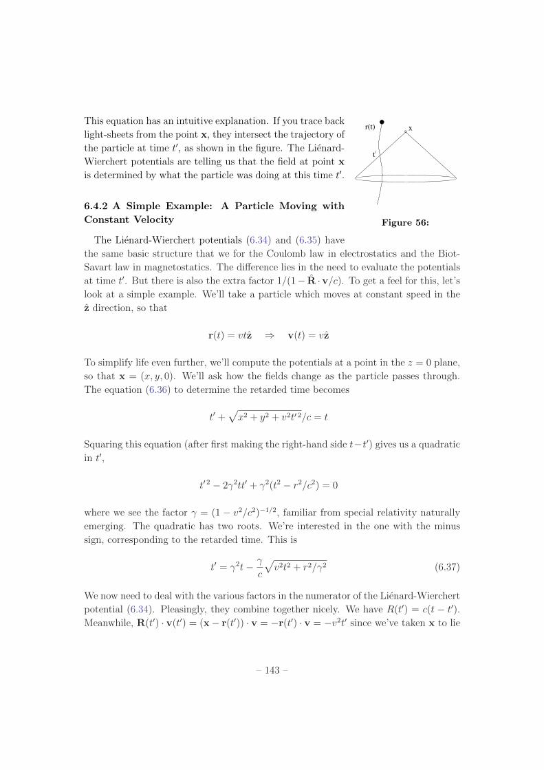
This equation has an intuitive explanation. If you trace backr(t) x

t/

Figure 56:

light-sheets from the point x, they intersect the trajectory of

the particle at time t0, as shown in the figure. The Lienard-

Wierchert potentials are telling us that the field at point x

is determined by what the particle was doing at this time t0.

6.4.2 A Simple Example: A Particle Moving with

Constant Velocity

The Lienard-Wierchert potentials (6.34) and (6.35) have

the same basic structure that we for the Coulomb law in electrostatics and the Biot-

Savart law in magnetostatics. The di↵erence lies in the need to evaluate the potentials

at time t0. But there is also the extra factor 1/(1 R ·v/c). To get a feel for this, let’s

look at a simple example. We’ll take a particle which moves at constant speed in the

z direction, so that

r(t) = vtz ) v(t) = vz

To simplify life even further, we’ll compute the potentials at a point in the z = 0 plane,

so that x = (x, y, 0). We’ll ask how the fields change as the particle passes through.

The equation (6.36) to determine the retarded time becomes

t0 +p

x2 + y2 + v2t0 2/c = t

Squaring this equation (after first making the right-hand side tt0) gives us a quadratic

in t0,

t0 2 22tt0 + 2(t2 r2/c2) = 0

where we see the factor = (1 v2/c2)1/2, familiar from special relativity naturally

emerging. The quadratic has two roots. We’re interested in the one with the minus

sign, corresponding to the retarded time. This is

t0 = 2t

c

pv2t2 + r2/2 (6.37)

We now need to deal with the various factors in the numerator of the Lienard-Wierchert

potential (6.34). Pleasingly, they combine together nicely. We have R(t0) = c(t t0).

Meanwhile, R(t0) · v(t0) = (x r(t0)) · v = r(t0) · v = v2t0 since we’ve taken x to lie

– 143 –

perpendicular to v. Put together, this gives us

(x, t) =q

40

1

[1 + v2t0/c(t t0)]

1

c(t t0)

=q

40

1

c(t t0) + v2t0

=1

40

1

c(t t0/2)

But, using our solution (6.37), this becomes

(x, t) =q

40

1

[v2t2 + (x2 + y2)/2]

Similarly, the vector potential is

A(x, t) =qµ

0

4

v

[v2t2 + (x2 + y2)/2]

How should we interpret these results? The distance from the particle to the point x is

r2 = x2+ y2+ v2t2. The potentials look very close to those due to a particle a distance

r away, but with one di↵erence: there is a contraction in the x and y directions. Of

course, we know very well what this means: it is the usual Lorentz contraction in special

relativity.

In fact, we previously derived the expression for the electric and magnetic field of a

moving particle in Section 5.3.4, simply by acting with a Lorentz boost on the static

fields. The calculation here was somewhat more involved, but it didn’t assume any rel-

ativity. Instead, the Lorentz contraction follows only by solving the Maxwell equations.

Historically, this kind of calculation is how Lorentz first encountered his contractions.

6.4.3 Computing the Electric and Magnetic Fields

We now compute the electric and magnetic fields due to a particle undergoing arbitrary

motion. In principle this is straightforward: we just need to take our equations (6.34)

and (6.35)

(x, t) =q

40

"c

c R(t0) · v(t0)1

R(t0)

#ret

A(x, t) =qµ

0

4

"c

c R(t0) · v(t0)v(t0)

R(t0)

#ret

where R(t0) = x r(t0). We then plug these into the standard expressions for the

electric field E = r @A/@t and the magnetic field B = r A. However, in

– 144 –

practice, this is a little fiddly. It’s because the terms in these equations are evaluated

at the retarded time t0 determined by the equation t0 + R(t0)/c = t. This means that

when we di↵erentiate (either by @/@t or by r), the retarded time also changes and

so gives a contribution. It turns out that it’s actually simpler to return to our earlier

expression (6.33),

(x, t) =q

40

Zdt0

1

R(t0)(t t0 R(t0)/c)

and a similar expression for the vector potential,

A(x, t) =qµ

0

4

Zdt0

v(t0)

R(t0)(t t0 R(t0)/c) (6.38)

This will turn out to be marginally easier to deal with.

The Electric Field

We start with the electric field E = r @A/@t. We call the argument of the

delta-function

s = t t0 R(t0)

We then have

r =q

40

Zdt0

rR

R2

(s) 1

R0(s)

rR

c

=

q

40

Zds

@t0@s

rR

R2

(s) rR

Rc0(s)

(6.39)

The Jacobian factor from changing the integral variable is the given by

@s

@t0= 1 + R(t0) · v(t0)/c

This quantity will appear a lot in what follows, so we give it a new name. We define

= 1 R(t0) · v(t0)/c

so that @t0/@s = 1/. Integrating the second term in (6.39) by parts, we can then

write

r =q

40

Zds

rR

R2

+d

ds

rR

Rc

(s)

=q

40

Zds

rR

R2

1

d

dt0

rR

Rc

(s)

– 145 –

Meanwhile, the vector potential term gives

@A

@t=

qµ0

4

Zdt0

v

R0(s)

@s

@t

But @s/@t = 1. Moving forward, we have

@A

@t=

qµ0

4

Zds

@t0@s

v

R0(s)

= qµ0

4

Zds

d

ds

v

R

(s)

=qµ

0

4

Zds

1

d

dt0

v

R

(s)

Putting this together, we get

E =q

40

Zds

rR

R2

+1

c

d

dt0

rR v/c

R

(s)

=q

40

"R

R2

+1

c

d

dt0

R v/c

R

!#ret

(6.40)

We’re still left with some calculations to do. Specifically, we need to take the derivative

d/dt0. This involves a couple of small steps. First,

dR

dt0=

d

dt0

R

R

= v

R+

R

R2

(R · v) = 1

R

v (v · R)R

Also,

d

dt0(R) =

d

dt0(RR · v/c) = v · R+ v2/cR · a/c

Putting these together, we get

d

dt0

R v/c

R

!= 1

R2

v v · R

a

Rc+

R v/c

2R2

v · R v2/c+R · a/c

We write the v · R terms as v · R = c(1 ). Then, expanding this out, we find that

a bunch of terms cancel, until we’re left with

d

dt0

R v/c

R

!= cR

R2

+c(R v/c)

2R2

(1 v2/c2) +1

2Rc

h(R v/c) R · a a

i= cR

R2

+c(R v/c)

22R2

+R [(R v/c) a]

2Rc(6.41)

– 146 –

where we’ve introduced the usual factor from special relativity: 2 = 1/(1 v2/c2).

Now we can plug this into (6.40) to find our ultimate expression for the electric field,

E(x, t) =q

40

"R v/c

23R2

+R [(R v/c) a]

3Rc2

#ret

(6.42)

Since it’s been a long journey, let’s recall what everything in this expression means.

The particle traces out a trajectory r(t), while we sit at some position x which is

where the electric field is evaluated. The vector R(t) is the di↵erence: R = x r.

The ret subscript means that we evaluate everything in the square brackets at time t0,

determined by the condition t0 +R(t0)/c = t. Finally,

= 1 R · vc

and 2 =1

1 v2/c2

The electric field (6.42) has two terms.

• The first term drops o↵ as 1/R2. This is what becomes of the usual Coulomb

field. It can be thought of as the part of the electric field that remains bound to

the particle. The fact that it is proportional to R, with a slight o↵-set from the

velocity, means that it is roughly isotropic.

• The second term drops o↵ as 1/R and is proportional to the acceleration. This

describes the radiation emitted by the particle. Its dependence on the acceleration

means that it’s highly directional.

The Magnetic Field

To compute the magnetic field, we start with the expression (6.38),

A(x, t) =qµ

0

4

Zdt0

v(t0)

R(t0)(s)

with s = t t0 R(t0)/c. Then, using similar manipulations to those above, we have

B = rA =qµ

0

4

Zdt0

rR

R2

v (s) +rs v

R0(s)

=

qµ0

4

Zds

rR

R2

v 1

d

dt0

rR v

Rc

(s) (6.43)

– 147 –

We’ve already done the hard work necessary to compute this time derivative. We can

write,

d

dt0

rR v

R

=

d

dt0

(R v/c) v

R

!

=d

dt0

R v/c

R

! v +

R v/c

R a

Now we can use (6.41). A little algebra shows that terms of the form va cancel, and

we’re left with

d

dt0

R v

R

!= cR v

R2

+cR v

22R2

+(R · a) R v

c2R2

+R a

R

Substituting this into (6.43), a little re-arranging of the terms gives us our final expres-

sion for the magnetic field,

B = qµ0

4

"R v

23R2

+(R · a)(R v/c) + R a

c3R

#ret

(6.44)

We see that this has a similar form to the electric field (6.42). The first term falls o↵ as

1/R2 and is bound to the particle. It vanishes when v = 0 which tells us that a charged

particle only gives rise to a magnetic field when it moves. The second term falls o↵ as

1/R. This is generated by the acceleration and describes the radiation emitted by the

particle. You can check that E in (6.42) and B in (6.44) are related through

B =1

c[R]

ret

E (6.45)

as you might expect.

6.4.4 A Covariant Formalism for Radiation

Before we make use of the Lienard-Wierchert potentials, we’re going to do something

a little odd: we’re going to derive them again. This time, however, we’ll make use of

the Lorentz invariant notation of electromagnetism. This won’t teach us anything new

about physics and the results of this section aren’t needed for what follows. But it will

give us some practice on manipulating these covariant quantities. Moreover, the final

result will be pleasingly concise.

– 148 –

A Covariant Retarded Potential

We start with our expression for the retarded potential (6.32) in terms of the current,

Aµ

(x, t) =µ0

4

Zd3x0 Jµ(x

0, tret

)

|x x0| (6.46)

with tret

= t|xx0|/c. This has been the key formula that we’ve used throughout this

section. Because it was derived from the Maxwell equations, this formula should be

Lorentz covariant, meaning that someone in a di↵erent inertial frame will write down

the same equation. Although this should be true, it’s not at all obvious from the way

that (6.46) is written that it actually is true. The equation involves only integration

over space, and the denominator depends only on the spatial distance between two

points. Neither of these are concepts that di↵erent observers agree upon.

So our first task is to rewrite (6.46) in a way which is manifestly Lorentz covariant.

To do this, we work with four-vectors Xµ = (ct,x) and take a quantity which everyone

agrees upon: the spacetime distance between two points

(X X 0)2 = µ

(Xµ X 0 )(Xµ X 0 ) = c2(t t0)2 |x x0|2

Consider the delta-function ((X X 0)2), which is non-vanishing only when X and

X 0 are null-separated. This is a Lorentz-invariant object. Let’s see what it looks like

when written in terms of the time coordinate t. We will need the general result for

delta-functions

(f(x)) =Xxi

(x xi

)

|f 0(xi

)| (6.47)

where the sum is over all roots f(xi

) = 0. Using this, we can write

(X X 0)2

= ([c(t0 t) + |x x0|][c(t0 t) |x x0|])=

(ct0 ct+ |x x0|)2c|t t0| +

(ct0 ct |x x0|)2c|t t0|

=(ct0 ct+ |x x0|)

2|x x0| +(ct0 ct |x x0|)

2|x x0|The argument of the first delta-function is ct0 ct

ret

and so this term contributes only

if t0 < t. The argument of the second delta-function is ct0 ctadv

and so this term can

contribute only contribute if t0 > t. But the temporal ordering of two spacetime points

is also something all observers agree upon, as long as those points are either timelike

or null separated. And here the delta-function requires the points to be null separated.

– 149 –

This means that if we picked just one of these terms, that choice would be Lorentz

invariant. Mathematically, we do this using the Heaviside step-function

(t t0) =

(1 t > t0

0 t < t0

We have

(X X 0)2

(t t0) =

(ct0 ctret

)

2|x x0| (6.48)

The left-hand side is manifestly Lorentz invariant. The right-hand side doesn’t look

Lorentz invariant, but this formula tells us that it must be! Now we can make use of

this to rewrite (6.46) in a way that the Lorentz covariance is obvious. It is

Aµ

(X) =µ0

2

Zd4X 0 J

µ

(X 0) (X X 0)2

(t t0) (6.49)

where the integration is now over spacetime, d4X 0 = c dt0 d3x0. The combination of

the delta-function and step-functions ensure that this integration is limited to the past

light-cone of a point.

A Covariant Current

Next, we want a covariant expression for the current formed by a moving charged

particle. We saw earlier that a particle tracing out a trajectory y(t) gives rise to a

charge density (6.30) and current (6.31) given by

(x, t) = q 3(x y(t)) and J(x, t) = q v(t) 3(x y(t)) (6.50)

(We’ve changed notation from r(t) to y(t) to denote the trajectory of the particle).

How can we write this in a manifestly covariant form?

We know from our course on Special Relativity that the best way to parametrise the

worldline of a particle is by using its proper time . We’ll take the particle to have

trajectory Y µ() = (ct(),y()). Then the covariant form of the current is

Jµ(X) = qc

Zd Y µ() 4(X Y ()) (6.51)

It’s not obvious that (6.51) is the same as (6.50). To see that it is, we can decompose

the delta-function as

4(X Y ()) = (ct Y 0()) 3(x y())

– 150 –

The first factor allows us to do the integral over d , but at the expense of picking up

a Jacobian-like factor 1/Y 0 from (6.47). We have

Jµ =qcY µ

Y 0

3(x y())

which does give us back the same expressions (6.50).

Covariant Lienard-Wierchert Potentials

We can now combine (6.49) and (6.51) to get the retarded potential,

Aµ(X) =µ0

qc

4

Zd4X 0

Zd Y µ() 4(X 0 Y ())

(ct0 ctret

)

|x x0|=

µ0

qc

4

Zd Y µ()

(ct Y 0() |x y()||x y()|

This remaining delta-function implicitly allows us to do the integral over proper time.

Using (6.48) we can rewrite it as

(ct Y 0() |x y()|)2|x y()| = (R() ·R())(R0()) (6.52)

where we’re introduced the separation 4-vector

Rµ = Xµ Y µ()

The delta-function and step-function in (6.52) pick out a unique value of the proper

time that contributes to the gauge potential at point X. We call this proper time ?

.

It is the retarded time lying along a null direction, R(?

) · R(?

) = 0. This should be

thought of as the proper time version of our previous formula (6.36).

The form (6.52) allows us to do the integral over . But we still pick up a Jacobian-

like factor from (6.47). This gives

(R() ·R())(R0()) =(

?

)

2|Rµ(?

)Y µ(?

)|Putting all of this together gives our covariant form for the Lienard-Wierchert potential,

Aµ(X) =µ0

qc

4

Y µ(?

)

|R(?

)Y

(?

)|This is our promised, compact expression. Expanding it out will give the previous

results for the scalar (6.34) and vector (6.35) potentials. (To see this, you’ll need to

first show that |R(?

)Y (?

)| = c(?

)R(?

)(1 R(?

) · v(?

)/c).)

– 151 –

The next step is to compute the field strength Fµ

= @µ

A

@

Aµ

. This is what

took us some time in Section 6.4.3. It turns out to be somewhat easier in the covariant

approach. We need to remember that ?

is a function of Xµ. Then, we get

Fµ

=µ0

qc

4

Y

(?

)

|R(?

)Y

(?

)|@

?

@Xµ

Y

(?

)

|R(?

)Y

(?

)|2@|R(

?

)Y

(?

)|@Xµ

! (µ $ ) (6.53)

The simplest way to compute @?

/@Xµ is to start with

R(?

)R(?

) = 0. Di↵eren-

tiating gives

R(?

)@µ

R(?

) =

R(?

)µ

Y (?

) @µ

?

= 0

Rearranging gives

@?

@Xµ

=R

µ

(?

)

R(?

)Y

(?

)

For the other term, we have

@|R(?

)Y

(?

)|@Xµ

=µ

Y (?

)@µ

?

Y

(?

) +R(?

)Y

(?

)@µ

?

=R(

?

)Y

(?

) + c2@µ

?

+ Yµ

(?

)

where we’ve used Y µYµ

= c2. Using these in (6.53), we get our final expression for

the field strength,

Fµ

(X) =µ0

qc

4

1

RY

"(c2 +RY

)R

µ

Y

R

Yµ

(RY

)2+

Yµ

R

Y

Rµ

RY

#(6.54)

This is the covariant field strength. It takes a little work to write this in terms of the

component E and B fields but the final answer is, of course, given by (6.42) and (6.44)

that we derived previously. Indeed, you can see the general structure in (6.54). The

first term is proportional to velocity and goes as 1/R2; the second term is proportional

to acceleration and goes as 1/R.

6.4.5 Bremsstrahlung, Cyclotron and Synchrotron Radiation

To end our discussion, we derive the radiation due to some simple relativistic motion.

Power Radiated Again: Relativistic Larmor Formula

In Section 6.2.2, we derived the Larmor formula for the emitted power in the electric

dipole approximation to radiation. In this section, we present the full, relativistic

version of this formula.

– 152 –

We’ll work with the expressions for the radiation fields E (6.42) and B (6.44). As

previously, we consider only the radiative part of the electric and magnetic fields which

drops o↵ as 1/R. The Poynting vector is

S =1

µ0

EB =1

µ0

cE (R E) =

1

µ0

c|E|2R

where all of these expressions are to be computed at the retarded time. The second

equality follows from the relation (6.45), while the final equality follows because the

radiative part of the electric field (6.42) is perpendicular to R. Using the expression

(6.42), we have

S =q2

1620

c3|R [(R v/c) a]|2

6R2

R

with = 1 R · v/c.Recall that everything in the formula above is evaluated at the retarded time t0,

defined by t0 +R(t0)/c = t. This means, that the coordinates are set up so that we can

integrate S over a sphere of radius R that surrounds the particle at its retarded time.

However, there is a subtlety in computing the emitted power, associated to the Doppler

e↵ect. The energy emitted per unit time t is not the same as the energy emitted per

unit time t0. They di↵er by the factor dt/dt0 = . The power emitted per unit time t0,

per solid angle d, is

dPd

= R2 S · R =q2

1620

c3|R [(R v/c) a]|2

5

(6.55)

To compute the emitted power, we must integrate this expression over the sphere. This

is somewhat tedious. The result is given by

P =q2

60

c34

a2 +

2

c2(v · a)2

(6.56)

This is the relativistic version of the Larmor formula (6.18). (There is a factor of 2

di↵erence when compared to (6.20) because the former equation was time averaged).

We now apply this to some simple examples.

Bremsstrahlung

Suppose a particle is travelling in a straight line, with velocity v parallel to acceleration

a. The most common situation of this type occurs when a particle decelerates. In this

case, the emitted radiation is called bremsstrahlung, German for “braking radiation”.

– 153 –

We’ll sit at some point x, at which the radiation reaches us from the retarded point

on the particle’s trajectory r(t0). As before, we define R(t0) = x r(t0). We introduce

the angle , defined by

R · v = v cos

Because the v a term in (6.55) vanishes, the angular dependence of the radiation is

rather simple in this case. It is given by

dPd

=q2a2

160

c3sin2

(1 (v/c) cos )5

For v c, the radiation is largest in the direction /2, perpendicular to the

direction of travel. But, at relativistic speeds, v ! c, the radiation is beamed in the

forward direction in two lobes, one on either side of the particle’s trajectory. The total

power emitted is (6.56) which, in this case, simplifies to

P =q26a2

60

c3

Cyclotron and Synchrotron Radiation

Suppose that the particle travels in a circle, with v · a = 0. We’ll pick axes so that a

is aligned with the x-axis and v is aligned with the z-axis. Then we write

R = sin cosx+ sin siny + cos z

After a little algebra, we find that the angular dependence of the emitted radiation is

dPd

=q2a2

160

c31

(1 (v/c) cos )3

1 sin2 cos2

2(1 (v/c) cos )2

At non-relativistic speeds, v c, the angular dependence takes the somewhat simpler

form (1 sin2 cos2 ). In this limit, the radiation is referred to as cyclotron radiation.

In contrast, in the relativistic limit v ! c, the radiation is again beamed mostly in the

forwards direction. This limit is referred to as synchrotron radiation. The total emitted

power (6.56) is this time given by

P =q24a2

60

c3

Note that the factors of di↵er from the case of linear acceleration.

– 154 –