6. Introduction to stochastic processes ...5 6. Introduction to stochastic processes Stochastic processes (3) • Each (individual) random variable Xt is a mapping from the sample

1Lect06.ppt S-38.145 - Introduction to Teletraffic Theory – Spring 2004

6. Introduction to stochastic processes

2


Contents

• Basic concepts

• Poisson process

• Markov processes• Birth-death processes

3


Stochastic processes (1)

• Consider some quantity in a teletraffic (or any) system

• It typically evolves in time randomly– Example 1: the number of occupied channels in a telephone link

at time t or at the arrival time of the nth customer

– Example 2: the number of packets in the buffer of a statistical multiplexer at time t or at the arrival time of the nth customer

• This kind of evolution is described by a stochastic process– At any individual time t (or n) the system can be described by a random

variable– Thus, the stochastic process is a collection of random variables

4



• Definition: A (real-valued) stochastic process X = (Xt | t ∈ I) is a collection of random variables Xt

– taking values in some (real-valued) set S, Xt(ω) ∈ S, and

– indexed by a real-valued (time) parameter t ∈ I.

• Stochastic processes are also called random processes(or just processes)

• The index set I ⊂ ℜ is called the parameter space of the process

• The value set S ⊂ ℜ is called the state space of the process

• Note: Sometimes notation Xt is used to refer to the whole stochastic process (instead of a single random variable related to the time t)

5



• Each (individual) random variable Xt is a mapping from the sample space Ω into the real values ℜ :

• Thus, a stochastic process X can be seen as a mapping from the sample space Ω into the set of real-valued functions ℜ I (with t ∈ I as an argument):

• Each sample point ω ∈ Ω is associated with a real-valued function X(ω). Function X(ω) is called a realization (or a path or a trajectory) of the process.

)( : ωω tt X,X ℜ→Ω

)( : ωω X,X Iℜ→Ω

6


Summary

• Given the sample point ω ∈ Ω– X(ω) = (Xt(ω) | t ∈ I) is a real-valued function (of t ∈ I)

• Given the time index t ∈ I, – Xt = (Xt(ω) | ω ∈ Ω ) is a random variable (as ω ∈ Ω )

• Given the sample point ω ∈ Ω and the time index t ∈ I,– Xt(ω) is a real value

7


Example

• Consider traffic process X = (Xt | t ∈ [0,T]) in a link between two telephone exchanges during some time interval [0,T]

– Xt denotes the number of occupied channels at time t

• Sample point ω ∈ Ω tells us

– what is the number X0 of occupied channels at time 0,

– what are the remaining holding times of the calls going on at time 0,

– at what times new calls arrive, and – what are the holding times of these new calls.

• From this information, it is possible to construct the realization X(ω) of the traffic process X

– Note that all the randomness in the process is included in the sample point ω– Given the sample point, the realization of the process is just a (deterministic)

function of time

8


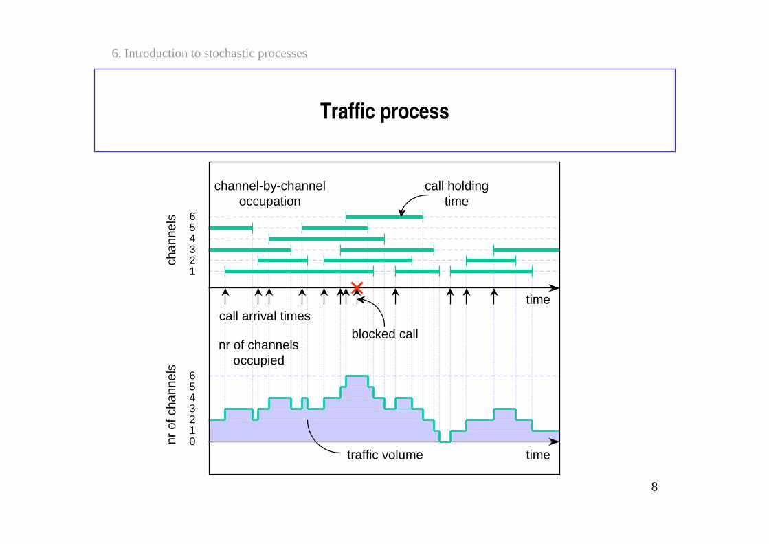
Traffic process

654321

6543210

time

time

call arrival timesblocked call

channel-by-channeloccupation

nr of channelsoccupied

traffic volume

call holdingtime

chan

nels

nr o

f cha

nnel

s

9


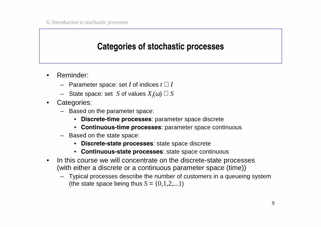
Categories of stochastic processes

• Reminder:– Parameter space: set I of indices t ∈ I– State space: set S of values Xt(ω) ∈ S

• Categories:– Based on the parameter space:

• Discrete-time processes: parameter space discrete• Continuous-time processes: parameter space continuous

– Based on the state space:• Discrete-state processes: state space discrete• Continuous-state processes: state space continuous

• In this course we will concentrate on the discrete-state processes (with either a discrete or a continuous parameter space (time))

– Typical processes describe the number of customers in a queueing system (the state space being thus S = 0,1,2,...)

10


Examples

• Discrete-time, discrete-state processes– Example 1: the number of occupied channels in a telephone link

at the arrival time of the nth customer, n = 1,2,...– Example 2: the number of packets in the buffer of a statistical multiplexer

at the arrival time of the nth customer, n = 1,2,...

• Continuous-time, discrete-state processes– Example 3: the number of occupied channels in a telephone link

at time t > 0– Example 4: the number of packets in the buffer of a statistical multiplexer

at time t > 0

11


Notation

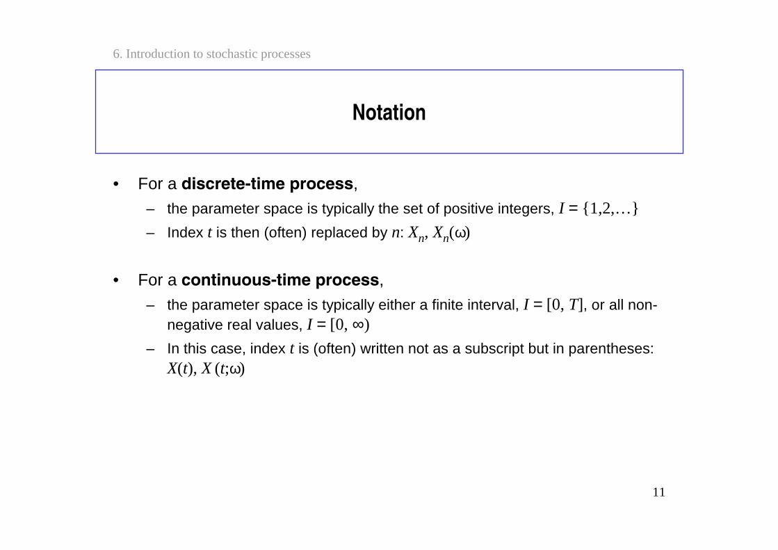
• For a discrete-time process,

– the parameter space is typically the set of positive integers, I = 1,2,…

– Index t is then (often) replaced by n: Xn, Xn(ω)

• For a continuous-time process,

– the parameter space is typically either a finite interval, I = [0, T], or all non-negative real values, I = [0, ∞)

– In this case, index t is (often) written not as a subscript but in parentheses: X(t), X (t;ω)

12


Distribution

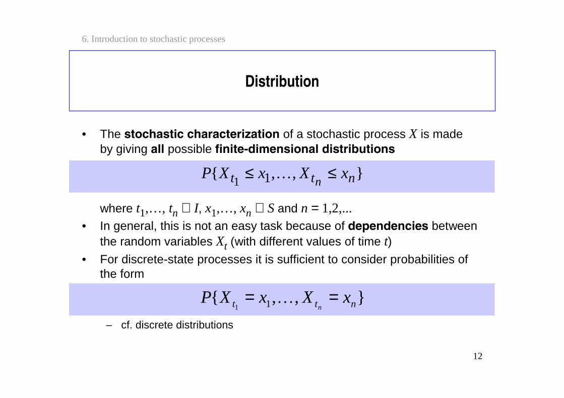
• The stochastic characterization of a stochastic process X is made by giving all possible finite-dimensional distributions

where t1,…, tn ∈ I, x1,…, xn ∈ S and n = 1,2,...• In general, this is not an easy task because of dependencies between

the random variables Xt (with different values of time t)• For discrete-state processes it is sufficient to consider probabilities of

the form

– cf. discrete distributions

,, 11 ntt xXxXPn

≤≤

,, 11 ntt xXxXPn

==

13


Dependence

• The most simple (but not so interesting) example of a stochasticprocess is such that all the random variables Xt are independent of each other. In this case

• The most simple non-trivial example is a discrete state Markov process. In this case

• This is related to the so called Markov property:– Given the current state (of the process),

the future (of the process) does not depend on the past (of the process), i.e. how the process has arrived to the current state

,..., 11 11 nttntt xXPxXPxXxXPnn

≤≤=≤≤

=== ,..., 11 ntt xXxXPn

|| 1121 1121 −====⋅=− ntntttt xXxXPxXxXPxXP

nn

14


Stationarity

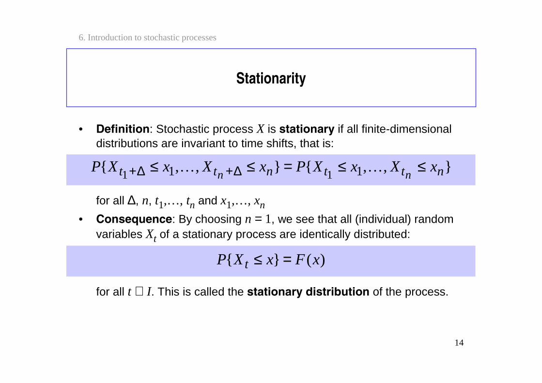
• Definition: Stochastic process X is stationary if all finite-dimensional distributions are invariant to time shifts, that is:

for all ∆, n, t1,…, tn and x1,…, xn

• Consequence: By choosing n = 1, we see that all (individual) random variables Xt of a stationary process are identically distributed:

for all t ∈ I. This is called the stationary distribution of the process.

,,,, 11 11 nttntt xXxXPxXxXPnn

≤≤=≤≤ ∆+∆+

)( xFxXP t =≤

15


Stochastic processes in teletraffic theory

• In this course (and, more generally, in teletraffic theory) various stochastic processes are needed to describe

– the arrivals of customers to the system (arrival process)

– the state of the system (state process)

• Note that the latter is also often called as traffic process

16


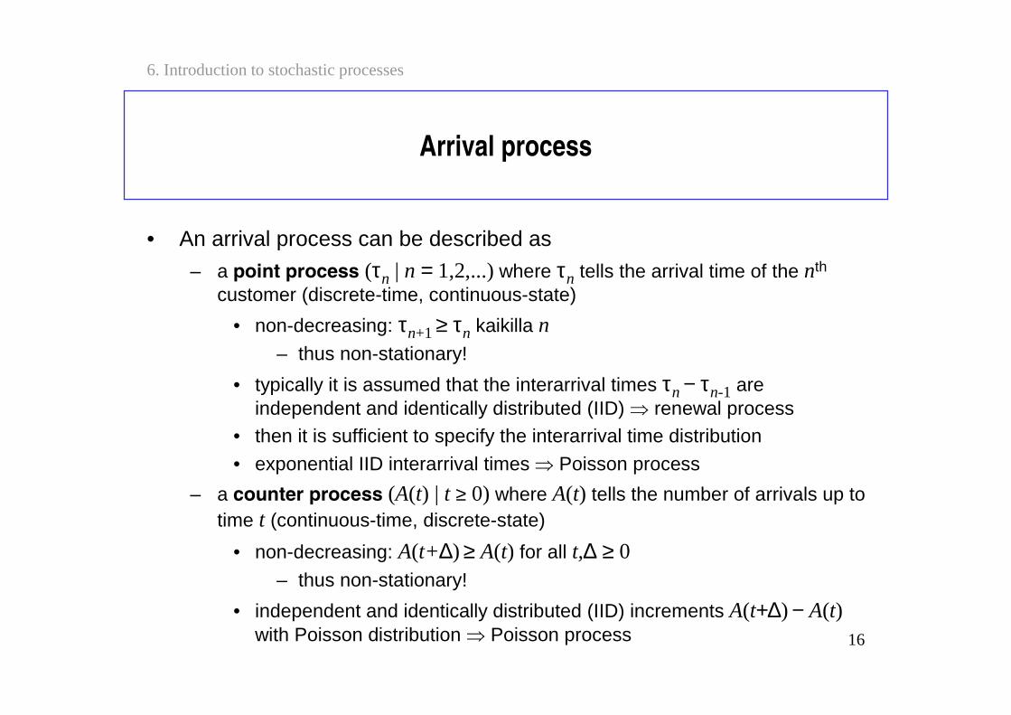
Arrival process

• An arrival process can be described as

– a point process (τn | n = 1,2,...) where τn tells the arrival time of the nth

customer (discrete-time, continuous-state)

• non-decreasing: τn+1 ≥ τn kaikilla n– thus non-stationary!

• typically it is assumed that the interarrival times τn − τn-1 are independent and identically distributed (IID) renewal process

• then it is sufficient to specify the interarrival time distribution

• exponential IID interarrival times Poisson process

– a counter process (A(t) | t ≥ 0) where A(t) tells the number of arrivals up to time t (continuous-time, discrete-state)

• non-decreasing: A(t+∆) ≥ A(t) for all t,∆ ≥ 0– thus non-stationary!

• independent and identically distributed (IID) increments A(t+∆) − A(t)with Poisson distribution Poisson process

17


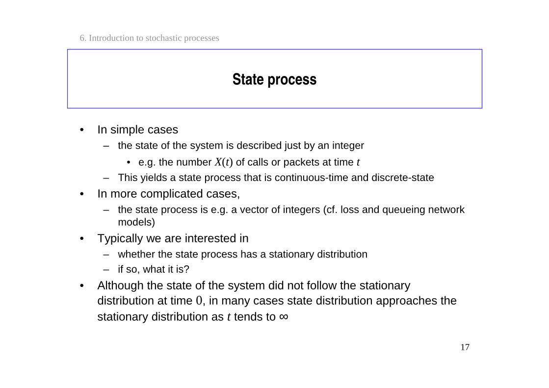
State process

• In simple cases – the state of the system is described just by an integer

• e.g. the number X(t) of calls or packets at time t– This yields a state process that is continuous-time and discrete-state

• In more complicated cases, – the state process is e.g. a vector of integers (cf. loss and queueing network

models)

• Typically we are interested in – whether the state process has a stationary distribution– if so, what it is?

• Although the state of the system did not follow the stationary distribution at time 0, in many cases state distribution approaches the stationary distribution as t tends to ∞

18


Contents

• Basic concepts

• Poisson process


19


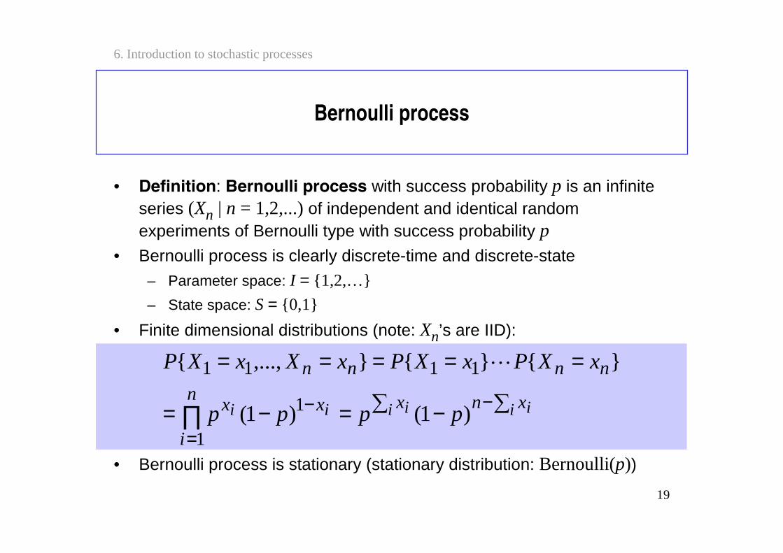
Bernoulli process

• Definition: Bernoulli process with success probability p is an infinite series (Xn | n = 1,2,...) of independent and identical random experiments of Bernoulli type with success probability p

• Bernoulli process is clearly discrete-time and discrete-state

– Parameter space: I = 1,2,…

– State space: S = 0,1

• Finite dimensional distributions (note: Xn’s are IID):

• Bernoulli process is stationary (stationary distribution: Bernoulli(p))

−=−=

=====

−

=

−∏ i ii iii xnxn

i

xx

nnnn

pppp

xXPxXPxXxXP

)1()1(

,...,

1

1

1111

20


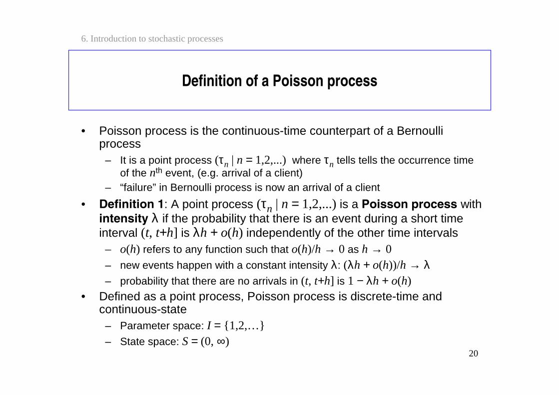
Definition of a Poisson process

• Poisson process is the continuous-time counterpart of a Bernoulli process

– It is a point process (τn | n = 1,2,...) where τn tells tells the occurrence time of the nth event, (e.g. arrival of a client)

– “failure” in Bernoulli process is now an arrival of a client

• Definition 1: A point process (τn | n = 1,2,...) is a Poisson process with intensity λ if the probability that there is an event during a short time interval (t, t+h] is λh + o(h) independently of the other time intervals– o(h) refers to any function such that o(h)/h → 0 as h → 0– new events happen with a constant intensity λ: (λh + o(h))/h → λ– probability that there are no arrivals in (t, t+h] is 1 − λh + o(h)

• Defined as a point process, Poisson process is discrete-time and continuous-state

– Parameter space: I = 1,2,…– State space: S = (0, ∞)

21


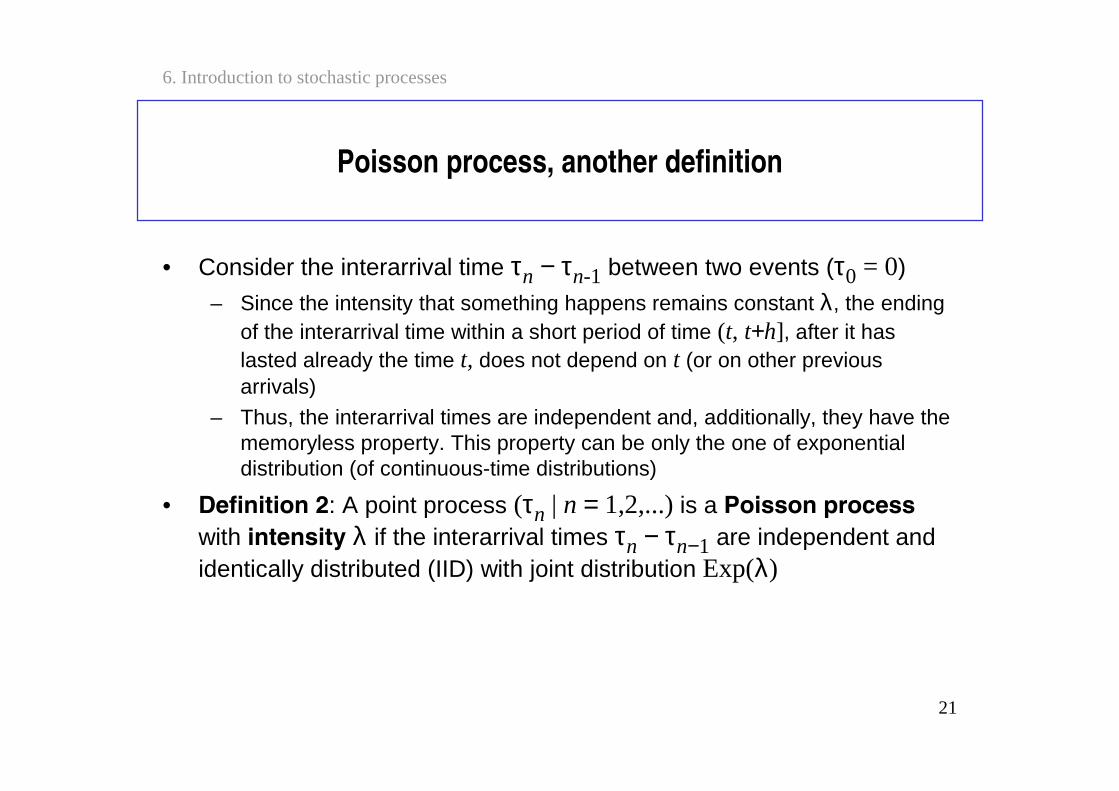
Poisson process, another definition

• Consider the interarrival time τn − τn-1 between two events (τ0 = 0)

– Since the intensity that something happens remains constant λ, the ending of the interarrival time within a short period of time (t, t+h], after it has lasted already the time t, does not depend on t (or on other previous arrivals)

– Thus, the interarrival times are independent and, additionally, they have the memoryless property. This property can be only the one of exponential distribution (of continuous-time distributions)

• Definition 2: A point process (τn | n = 1,2,...) is a Poisson processwith intensity λ if the interarrival times τn − τn−1 are independent and identically distributed (IID) with joint distribution Exp(λ)

22


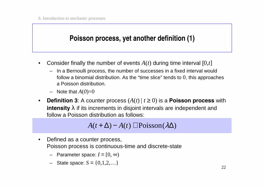
Poisson process, yet another definition (1)

• Consider finally the number of events A(t) during time interval [0,t]– In a Bernoulli process, the number of successes in a fixed interval would

follow a binomial distribution. As the “time slice” tends to 0, this approaches a Poisson distribution.

– Note that A(0)=0

• Definition 3: A counter process (A(t) | t ≥ 0) is a Poisson process with intensity λ if its increments in disjoint intervals are independent and follow a Poisson distribution as follows:

• Defined as a counter process, Poisson process is continuous-time and discrete-state

– Parameter space: I = [0, ∞)

– State space: S = 0,1,2,…

)(Poisson)()( ∆∼−∆+ λtAtA

23


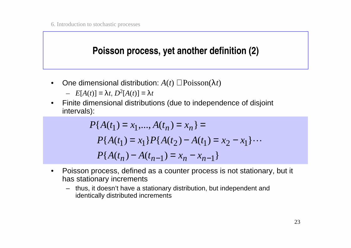
Poisson process, yet another definition (2)

• One dimensional distribution: A(t) ∼ Poisson(λt)– E[A(t)] = λt, D2[A(t)] = λt

• Finite dimensional distributions (due to independence of disjoint intervals):

• Poisson process, defined as a counter process is not stationary, but it has stationary increments

– thus, it doesn’t have a stationary distribution, but independent and identically distributed increments

)()(

)()()(

)(,...,)(

11

121211

11

−− −=−−=−=

===

nnnn

nn

xxtAtAP

xxtAtAPxtAP

xtAxtAP

24


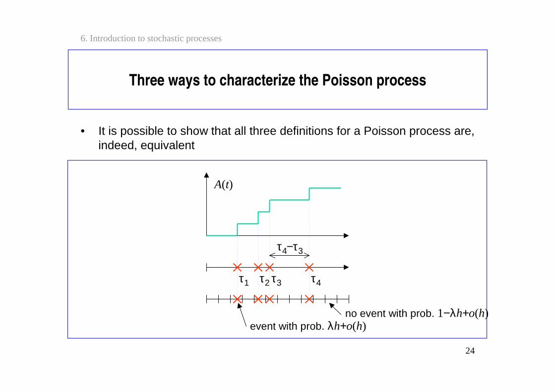
Three ways to characterize the Poisson process

• It is possible to show that all three definitions for a Poisson process are, indeed, equivalent

A(t)

τ1 τ2 τ3 τ4

τ4−τ3

event with prob. λh+o(h)no event with prob. 1−λh+o(h)

25


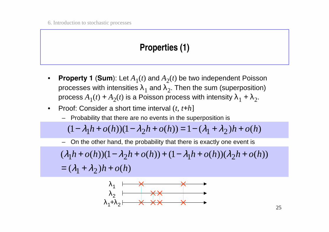
Properties (1)

• Property 1 (Sum): Let A1(t) and A2(t) be two independent Poisson processes with intensities λ1 and λ2. Then the sum (superposition) process A1(t) + A2(t) is a Poisson process with intensity λ1 + λ2.

• Proof: Consider a short time interval (t, t+h]– Probability that there are no events in the superposition is

– On the other hand, the probability that there is exactly one event is

)()(1))(1))((1( 2121 hohhohhoh ++−=+−+− λλλλ

))())((1())(1))((( 2121 hohhohhohhoh ++−++−+ λλλλ

λ1λ2

λ1+λ2

)()( 21 hoh ++= λλ

26


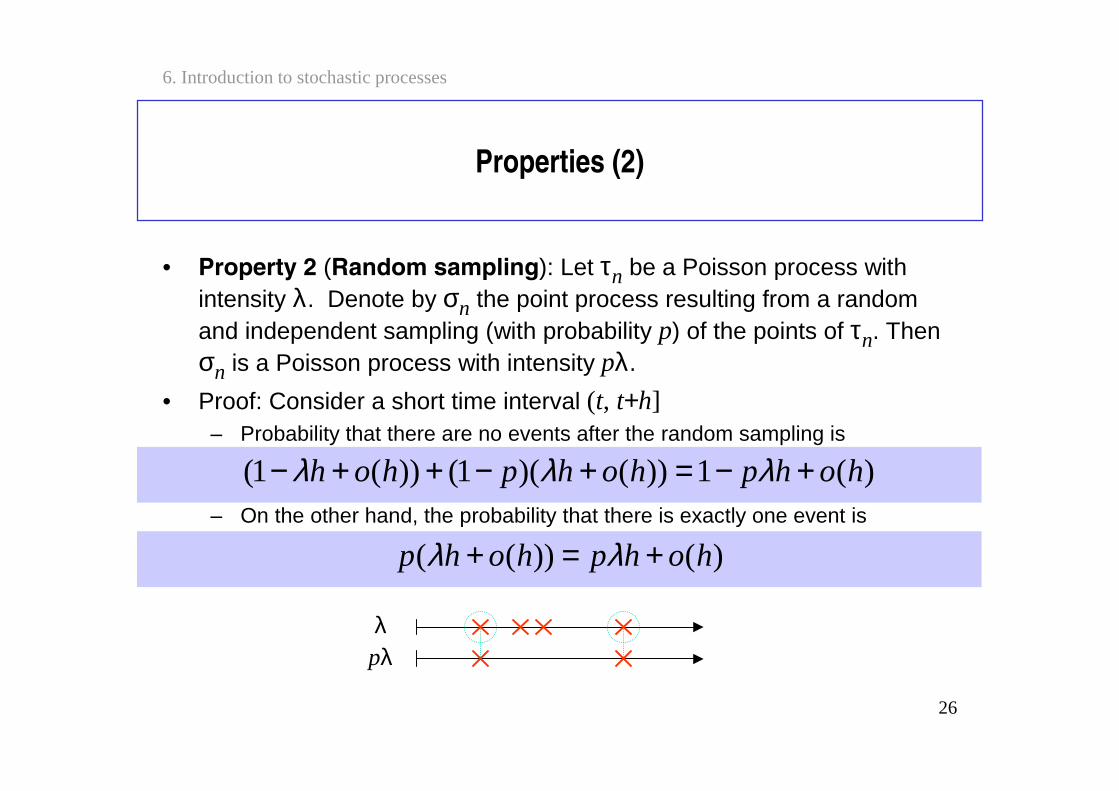
Properties (2)

• Property 2 (Random sampling): Let τn be a Poisson process with intensity λ. Denote by σn the point process resulting from a random and independent sampling (with probability p) of the points of τn. Then σn is a Poisson process with intensity pλ.

• Proof: Consider a short time interval (t, t+h]– Probability that there are no events after the random sampling is

– On the other hand, the probability that there is exactly one event is

)(1))()(1())(1( hohphohphoh +−=+−++− λλλ

)())(( hohphohp +=+ λλ

λpλ

27


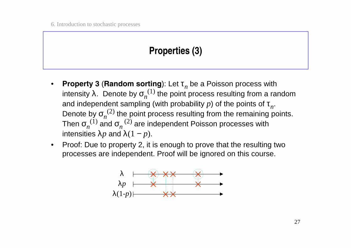
Properties (3)

• Property 3 (Random sorting): Let τn be a Poisson process with intensity λ. Denote by σn

(1) the point process resulting from a random and independent sampling (with probability p) of the points of τn. Denote by σn

(2) the point process resulting from the remaining points. Then σn

(1) and σn(2) are independent Poisson processes with

intensities λp and λ(1 − p). • Proof: Due to property 2, it is enough to prove that the resulting two

processes are independent. Proof will be ignored on this course.

λλp

λ(1-p)

28


Properties (4)

• Property 4 (PASTA): Consider any simple (and stable) teletrafficmodel with Poisson arrivals. Let X(t) denote the state of system at time t (continuous-time process) and Yn denote the state of the system seen by the nth arriving customer (discrete-time process). Then the stationary distribution of X(t) is the same as the stationary distribution of Yn.

• Thus, we can say that – arriving customers see the system in the stationary state– PASTA= “Poisson Arrivals See Time Avarages”

• PASTA property is only valid for Poisson arrivals– and it is not valid for other arrival processes– consider e.g. your own PC. Whenever you start a new session, the system

is idle. In the continuous time, however, the system is not only idle but also busy (when you use it).

29


Contents

• Basic concepts

• Poisson process


30


Markov process

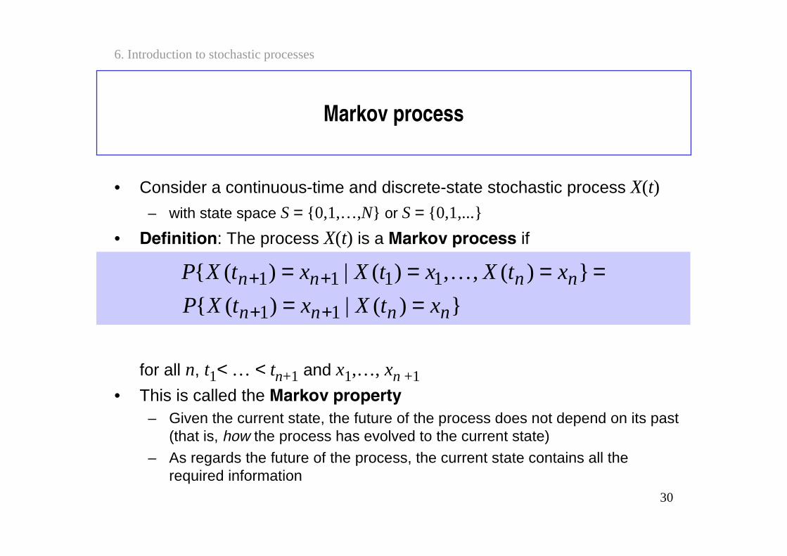
• Consider a continuous-time and discrete-state stochastic process X(t)– with state space S = 0,1,…,N or S = 0,1,...

• Definition: The process X(t) is a Markov process if

•

for all n, t1< … < tn+1 and x1,…, xn +1• This is called the Markov property

– Given the current state, the future of the process does not depend on its past (that is, how the process has evolved to the current state)

– As regards the future of the process, the current state contains all the required information

==== ++ )(,,)(|)( 1111 nnnn xtXxtXxtXP

)(|)( 11 nnnn xtXxtXP == ++

31


Example

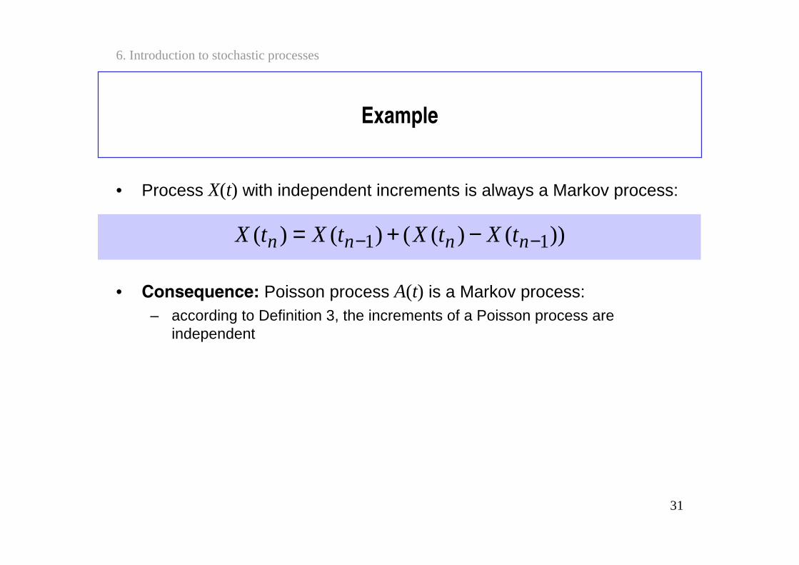
• Process X(t) with independent increments is always a Markov process:

• Consequence: Poisson process A(t) is a Markov process:– according to Definition 3, the increments of a Poisson process are

independent

))()(()()( 11 −− −+= nnnn tXtXtXtX

32


Time-homogeneity

• Definition: Markov process X(t) is time-homogeneous if

for all t, ∆ ≥ 0 and x, y ∈ S– In other words,

probabilities PX(t + ∆) = y | X(t) = x are independent of t

)0(|)()(|)( xXyXPxtXytXP ==∆===∆+

33


State transition rates

• Consider a time-homogeneous Markov process X(t)

• The state transition rates qij, where i, j ∈ S, are defined as follows:

• The initial distribution PX(0) = i, i ∈ S, and the state transition ratesqij together determine the state probabilities PX(t) = i, i ∈ S, by theKolmogorov (backwards/forwards) equations

• Note that on this course we will consider only time-homogeneous Markov processes

)0(|)(lim: 1

0iXjhXPq

hhij ===

↓

34


Exponential holding times

• Assume that a Markov process is in state i• During a short time interval (t, t+h] , the conditional probability that there

is a transition from state i to state j is qijh + o(h) (independently of the other time intervals)

• Let qi denote the total transition rate out of state i, that is:

• Then, during a short time interval (t, t+h] , the conditional probability that there is a transition from state i to any other state is qih + o(h)(independently of the other time intervals)

• This is clearly a memoryless property• Thus, the holding time in (any) state i is exponentially distributed with

intensity qi

≠

=ij

iji qq :

35


State transition probabilities

• Let Ti denote the holding time in state i and Tij denote the (potential) holding time in state i that ends to a transition to state j

• Ti can be seen as the minimum of independent and exponentially distributed holding times Tij (see lecture 5, slide 44)

• Let then pij denote the conditional probability that, when in state i, there is a transition from state i to state j (the state transition probabilities);

ijij

i TT≠

= min

i

ijijiij q

qTTPp ===

)(Exp ,)(Exp ijijii qTqT ∼∼

36


State transition diagram

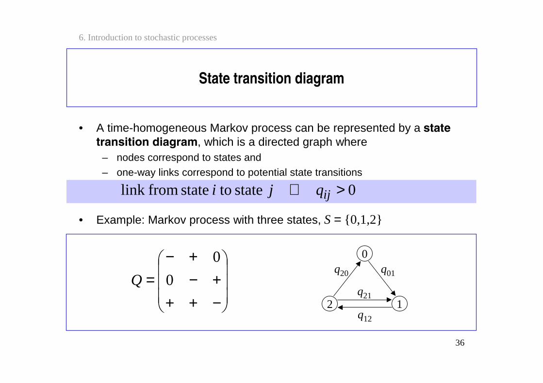
• A time-homogeneous Markov process can be represented by a state transition diagram, which is a directed graph where

– nodes correspond to states and

– one-way links correspond to potential state transitions

• Example: Markov process with three states, S = 0,1,2

0 statetostatefromlink >⇔ ijqji

2

0

1

q20 q01

q21

q12

−+++−

+−= 0

0

Q

37


Irreducibility

• Definition: There is a path from state i to state j (i → j) if there is a directed path from state i to state j in the state transition diagram.

– In this case, starting from state i, the process visits state j with positive probability (sometimes in the future)

• Definition: States i and j communicate (i ↔ j) if i → j and j → i.

• Definition: Markov process is irreducible if all states i ∈ Scommunicate with each other

– Example: The Markov process presented in the previous slide is irreducible

38


Global balance equations and equilibrium distributions

• Consider an irreducible Markov process X(t), with state transition rates qij

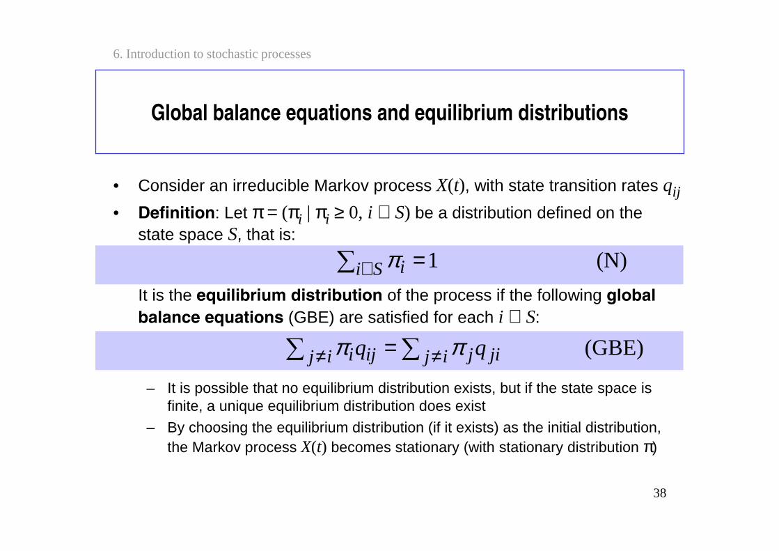
• Definition: Let π =(πi | πi ≥ 0, i ∈ S) be a distribution defined on the state space S, that is:

It is the equilibrium distribution of the process if the following global balance equations (GBE) are satisfied for each i ∈ S:

– It is possible that no equilibrium distribution exists, but if the state space is finite, a unique equilibrium distribution does exist

– By choosing the equilibrium distribution (if it exists) as the initial distribution, the Markov process X(t) becomes stationary (with stationary distribution π)

(N) 1= ∈ Si iπ

(GBE) ≠≠ = ij jijij iji qq ππ

39


Example

2

0

1

1 1

µ

1

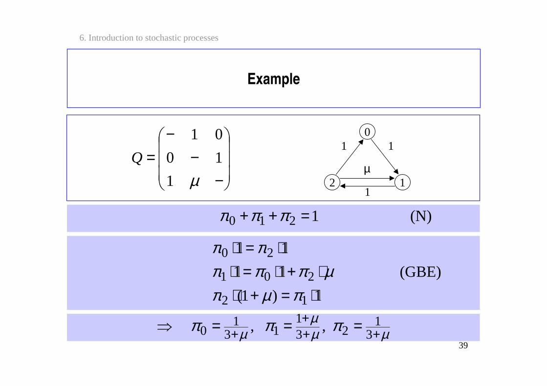
(N) 1210 =++ πππ

1)1(

(GBE) 1 1

11

12

201

20

⋅=+⋅⋅+⋅=⋅

⋅=⋅

πµπµπππ

ππ

µµµ

µ πππ +++

+ ===3

123

113

10 , ,

−−

−=

µ1

10

01

Q

40


Local balance equations

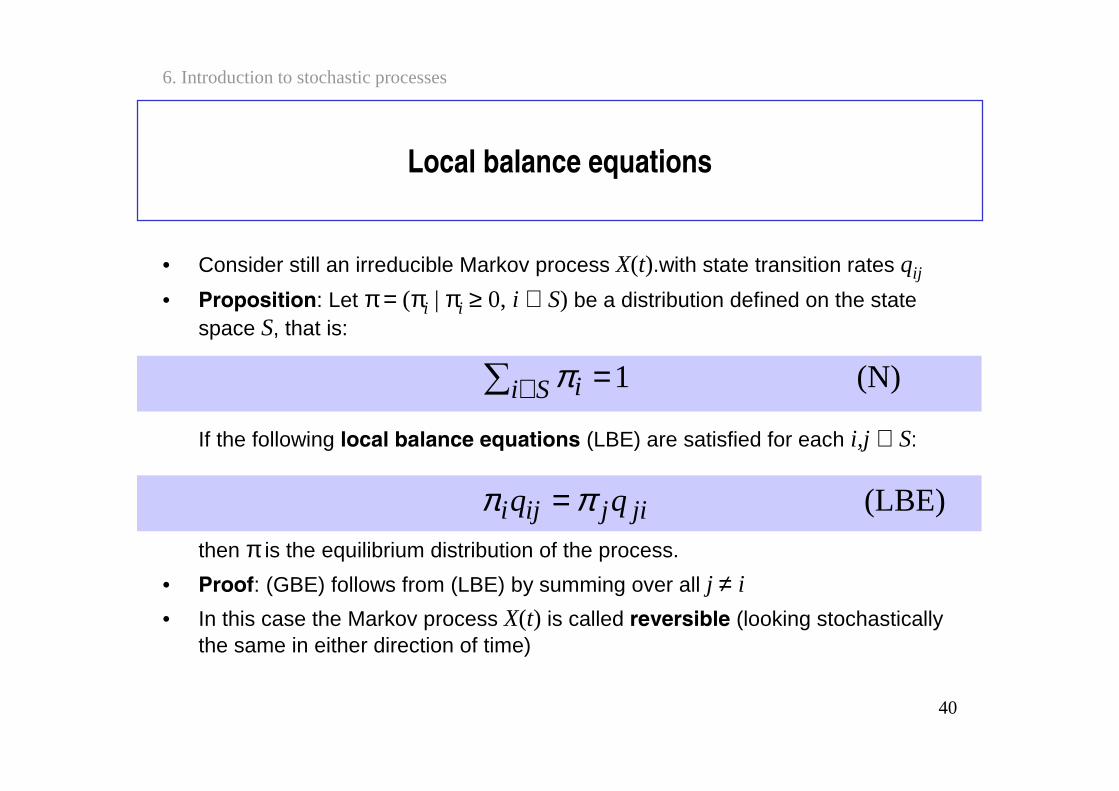
• Consider still an irreducible Markov process X(t).with state transition rates qij

• Proposition: Let π =(πi | πi ≥ 0, i ∈ S) be a distribution defined on the state space S, that is:

•

If the following local balance equations (LBE) are satisfied for each i,j ∈ S:

•then π is the equilibrium distribution of the process.

• Proof: (GBE) follows from (LBE) by summing over all j ≠ i

• In this case the Markov process X(t) is called reversible (looking stochastically the same in either direction of time)

(N) 1= ∈ Si iπ

(LBE) jijiji qq ππ =

41


Contents

• Basic concepts

• Poisson process


42


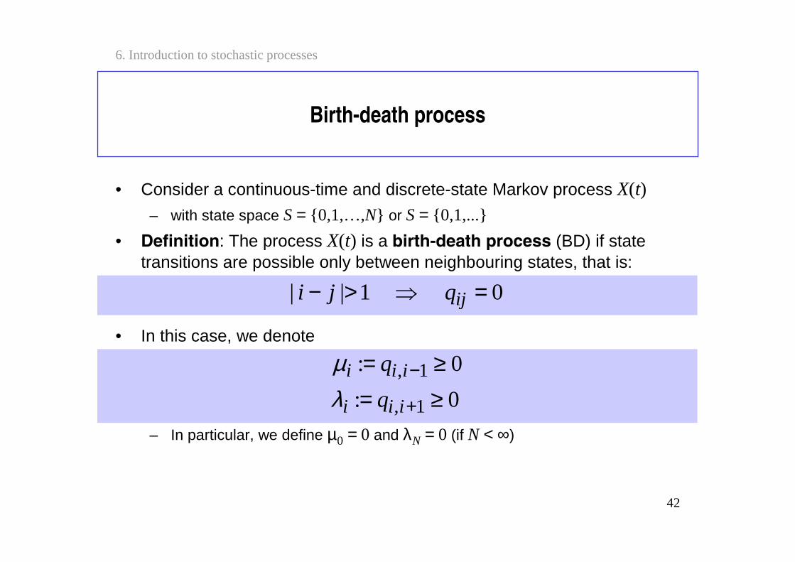
Birth-death process

• Consider a continuous-time and discrete-state Markov process X(t)– with state space S = 0,1,…,N or S = 0,1,...

• Definition: The process X(t) is a birth-death process (BD) if state transitions are possible only between neighbouring states, that is:

• In this case, we denote

– In particular, we define µ0 = 0 and λN = 0 (if N < ∞)

0 1|| =>− ijqji

0: 1, ≥= −iii qµ0: 1, ≥= +iii qλ

43


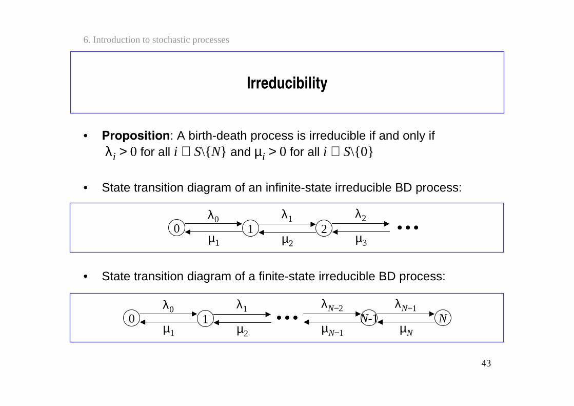
Irreducibility

• Proposition: A birth-death process is irreducible if and only if λi > 0 for all i ∈ S\N and µi > 0 for all i ∈ S\0

• State transition diagram of an infinite-state irreducible BD process:

• State transition diagram of a finite-state irreducible BD process:

1 2λ1

µ2

0λ0

µ1

λ2

µ3

1 N-1λ1

µ2

0λ0

µ1

λN−2

µN−1

NλN−1

µN

44


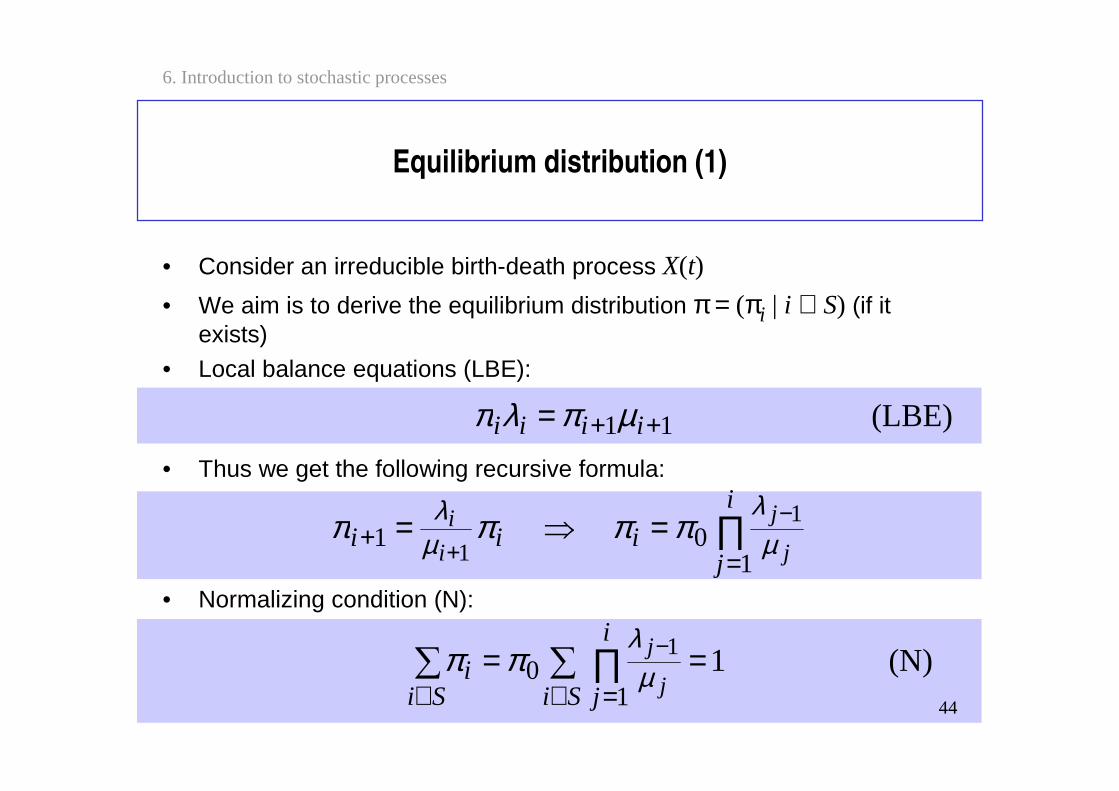
Equilibrium distribution (1)

• Consider an irreducible birth-death process X(t)

• We aim is to derive the equilibrium distribution π =(πi | i ∈ S) (if it exists)

• Local balance equations (LBE):

• Thus we get the following recursive formula:

• Normalizing condition (N):

(LBE) 11 ++= iiii µπλπ

∏=

+−

+==

i

jiii

j

j

i

i

101

1

1 µ

λµλ ππππ

(N) 11

01 == ∏

∈ =∈

−

Si

i

jSii

j

jµ

λππ

44

45


1

1 10

10

11 1 ,

−∞

= ==

+== ∏∏ −−

i

i

j

i

ji

j

j

j

jµ

λµ

λπππ

Equilibrium distribution (2)

• Thus, the equilibrium distribution exists if and only if

• Finite state space: The sum above is always finite, and the equilibrium distribution is

• Infinite state space: If the sum above is finite, the equilibrium distribution is

∞< ∏∈ =

−

Si

i

j j

j

1

1µ

λ

1

1 10

10

11 1 ,

−

= ==

+== ∏∏ −− N

i

i

j

i

ji

j

j

j

jµ

λµ

λπππ

45

46


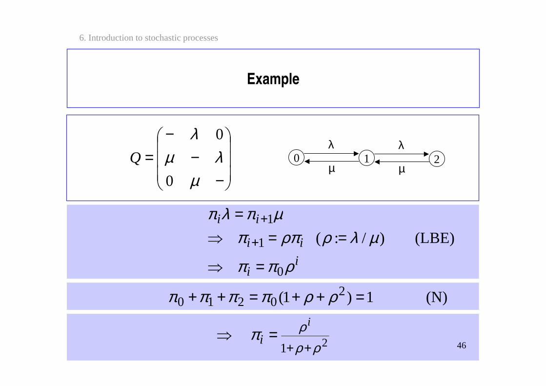
Example

1 2λ

µ

(N) 1)1( 20210 =++=++ ρρππππ

ii

ii

ii

ρππ

µλρρππµπλπ

0

1

1

(LBE) )/:(

=

==

=

+

+

21

ρρρπ++

=

i

i

0λ

µ

46

−−

−=

µλµ

λ

0

0

Q

47


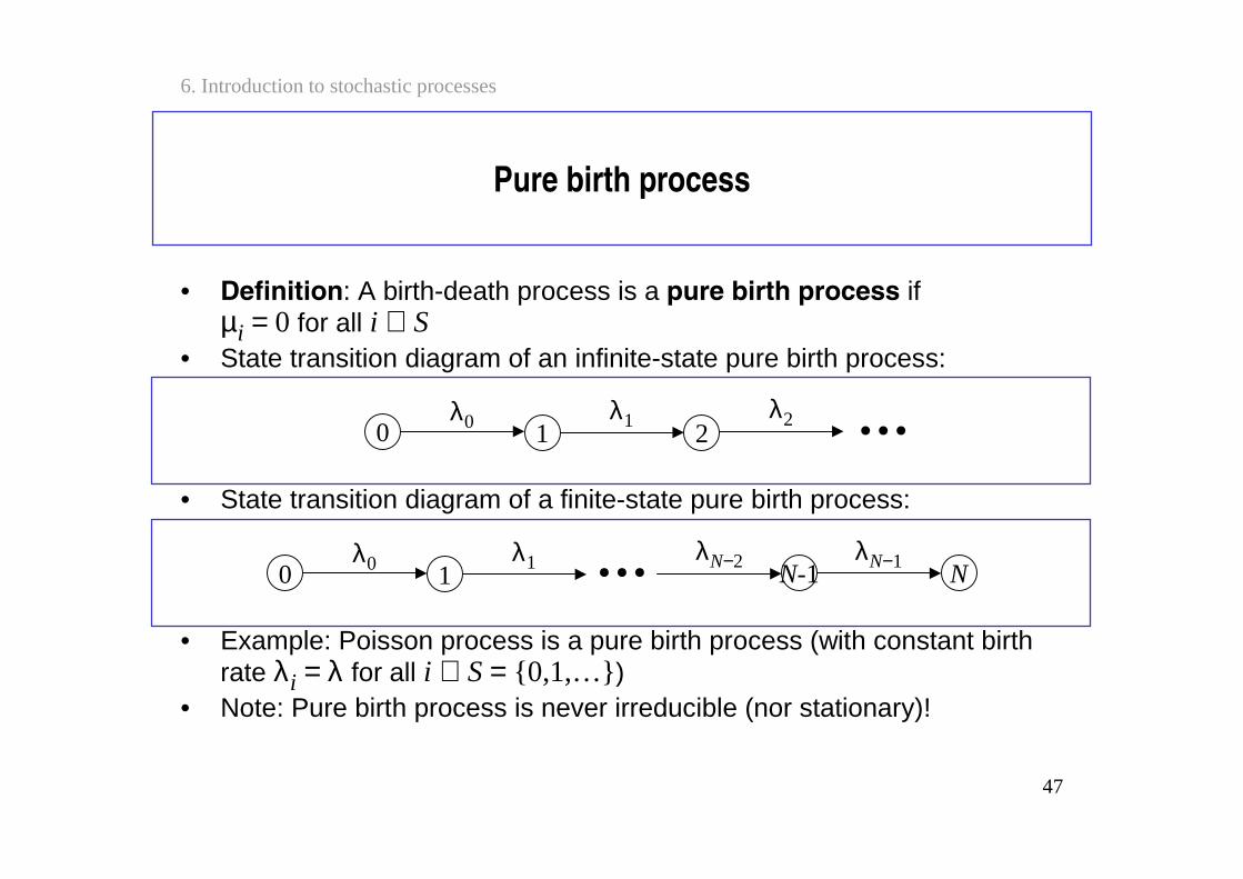
Pure birth process

• Definition: A birth-death process is a pure birth process ifµi = 0 for all i ∈ S

• State transition diagram of an infinite-state pure birth process:

• State transition diagram of a finite-state pure birth process:

• Example: Poisson process is a pure birth process (with constant birth rate λi = λ for all i ∈ S = 0,1,…)

• Note: Pure birth process is never irreducible (nor stationary)!

1 2λ10

λ0 λ2

1 N-1λ10

λ0 λN−2N

λN−1

Documents

6. Introduction to stochastic processes ...5 6. Introduction to stochastic processes Stochastic processes (3) • Each (individual) random variable Xt is a mapping from the sample