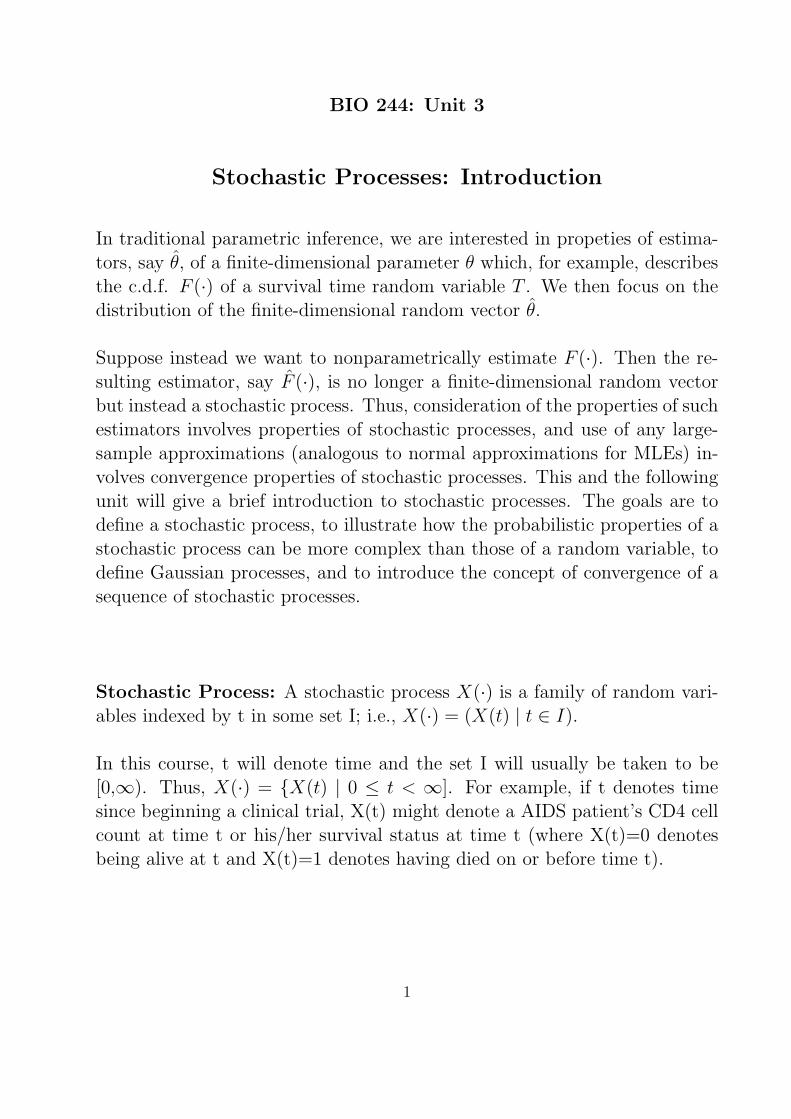
BIO 244: Unit 3

Stochastic Processes: Introduction

In traditional parametric inference, we are interested in propeties of estima-tors, say θ, of a finite-dimensional parameter θ which, for example, describesthe c.d.f. F (·) of a survival time random variable T . We then focus on thedistribution of the finite-dimensional random vector θ.

Suppose instead we want to nonparametrically estimate F (·). Then the re-sulting estimator, say F (·), is no longer a finite-dimensional random vectorbut instead a stochastic process. Thus, consideration of the properties of suchestimators involves properties of stochastic processes, and use of any large-sample approximations (analogous to normal approximations for MLEs) in-volves convergence properties of stochastic processes. This and the followingunit will give a brief introduction to stochastic processes. The goals are todefine a stochastic process, to illustrate how the probabilistic properties of astochastic process can be more complex than those of a random variable, todefine Gaussian processes, and to introduce the concept of convergence of asequence of stochastic processes.

Stochastic Process: A stochastic process X(·) is a family of random vari-ables indexed by t in some set I; i.e., X(·) = (X(t) | t ∈ I).

In this course, t will denote time and the set I will usually be taken to be[0,∞). Thus, X(·) = X(t) | 0 ≤ t < ∞]. For example, if t denotes timesince beginning a clinical trial, X(t) might denote a AIDS patient’s CD4 cellcount at time t or his/her survival status at time t (where X(t)=0 denotesbeing alive at t and X(t)=1 denotes having died on or before time t).

1

Commonly, the value, X(t), of the process X(·) at time t is referred to as the“state of the process” at time t. One way of describing a stochastic processX(·) is by the qualitative nature of the set I or of the values of X(t). Thefollowing categories are sometimes used:

Type of Process

X(t) = concentration of a drug in theblood t time units after ad-ministration

CT, CS

X(t) = air pollution level on day t DT, CSX(t) = # asthma attacks that occur

by time t since beginning atreatment

CT, DS

X(t) = indicator of a drug-resistantmutation at codon site t

DT, DS

CT : continuous timeDT : discrete timeCS : continuous stateDS : discrete state

Our focus in this course will be on continuous time processes, usually withdiscrete states (CT, DS).

Because X(·) is a family of random variables, descriptions of the propertiesof a stochastic process tend to be more complicated than those of a scalarrandom variable. To see this, recall that realizations of a scalar randomvariable Y can be viewed as arising from a mapping from a space Ω to thereal line; i.e.,

Y : Ω → R.

For example, we view realizations (observations) from the random variableY as mappings of different points in Ω; e.g., we might have Y(ω1)=6.5 andY(ω2)=14.1, where ω1 and ω2 are two points in Ω.

2

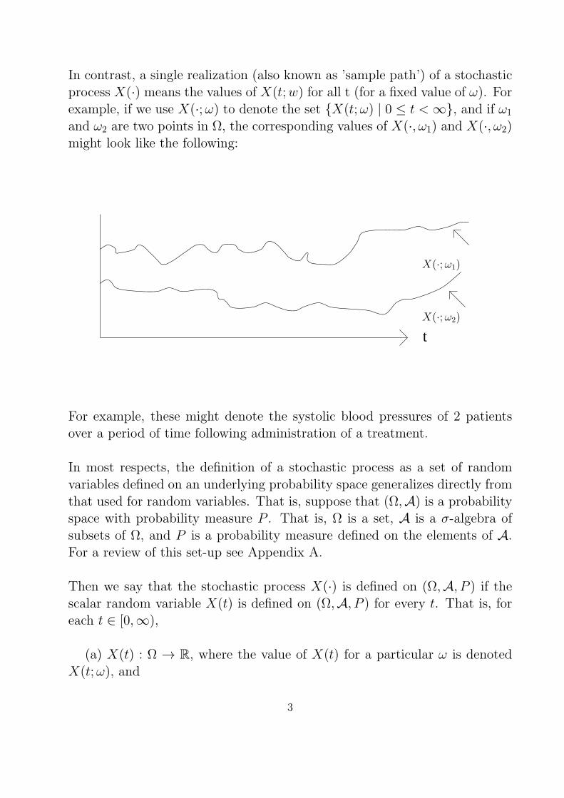
In contrast, a single realization (also known as ’sample path’) of a stochasticprocess X(·) means the values of X(t;w) for all t (for a fixed value of ω). Forexample, if we use X(·;ω) to denote the set X(t;ω) | 0 ≤ t < ∞, and if ω1

and ω2 are two points in Ω, the corresponding values of X(·, ω1) and X(·, ω2)might look like the following:

t

X(·;ω1)

X(·;ω2)

For example, these might denote the systolic blood pressures of 2 patientsover a period of time following administration of a treatment.

In most respects, the definition of a stochastic process as a set of randomvariables defined on an underlying probability space generalizes directly fromthat used for random variables. That is, suppose that (Ω,A) is a probabilityspace with probability measure P . That is, Ω is a set, A is a σ-algebra ofsubsets of Ω, and P is a probability measure defined on the elements of A.For a review of this set-up see Appendix A.

Then we say that the stochastic process X(·) is defined on (Ω,A, P ) if thescalar random variable X(t) is defined on (Ω,A, P ) for every t. That is, foreach t ∈ [0,∞),

(a) X(t) : Ω → R, where the value of X(t) for a particular ω is denotedX(t;ω), and

3

(b) X(t) is measurable: for any x ∈ R, the set E(x, t)def= ω ∈ Ω :

X(t, ω) ≤ x ∈ A.

Let’s consider the analogs of these properties for the entire stochastic processX(·). The analog of (a) is the function

X(·;ω) def= X(t;ω) : 0 ≤ t < ∞ ,

a ”sample path” of the process X(·). Thus, when we are dealing with a ran-dom variable X, we sometimes think of a set of n realizations as the valuesXi(ω) for i=1,2,...,n where ω ∈ Ω. In contrast, n realizations or sample pathsfrom the stochastic process X(·) are the values of the n functions Xi(·;ω),for i=1,2,...,n.

Now consider (b); that is, that the scalar random variableX(t) isA-measurable.It is tempting to conclude from (b) that any event expressible in terms ofX(·)is A-measurable, which would be desirable because otherwise the probabilityof such events would not be defined. However, this need not be the case.For any two times, say t1 and t2, consider the random variables X(t1) andX(t2). Then for any reals x1 and x2, the measurability of X(t1) and X(t2)ensures that E(x1, t1) and E(x2, t2) are elements of A, and hence the eventE = E(x1, t1)∩E(x2, t2) is also an element of A. Similar arguments hold forthe k random variables formed by examining X(·) at k distinct time points,or for that matter for a countably infinite number of random variables sinceσ-algebras are closed under countably infinite intersections. However, sinceX(·) contains an uncountably infinite number of random variables, complica-tions can arise because events desribed in terms of values of the process maynot correspond to elements of the σ-algebra A, in which case the probabilityof the event would not be defined. This is illustrated in the following example.

Example 3.1: Suppose that (Ω,A, P ) is the unit interval probability space(see Appendix A), I = [0, 1], and S is some non-measurable subset of Ω =[0, 1]. Define the stochastic process X(·) by X(t;ω) = 1 if ω ∈ S and ω = t,and X(t;ω) = 0 otherwise. Then it can be verified that X(t) is A-measurablefor every t. However, consider the event

4

Edef= ω : sup

tX(t;ω) ≤ 0.

Since P (X(t) = 0) = 1 for every t, we would want to consider E as an eventand to take its probability to be 1. However, E = Ω\S, which is not ameasurable set. Therefore, we cannot consider E as an event and take itsprobability to be 1, because the probability measure P is only defined onelements of A.

Some Definitions and Results

• X(·) = X(t), tϵI called continuous if P [A] = 1,

where A = ω : X(·; ω) is a continuous function of tϵI

Similar definitions for right continuous and left continuous.

−→ i.e., the stochastic process is said to have the property if the setof its sample paths which have the property has probability 1.

We now consider 2 definitions of relationships between processes (takenfrom Fleming & Harrington, 1991).

• X(·) and Y (·) are indistinguishable if P [B] = 1,

where B = ωϵΩ : X(t;ω) = Y (t;ω) for all tϵI

• X(·) is a modification of Y (·)if, for every tϵI, P [X(t) = Y (t)] = 1

i.e., if for every t, P [Ct] = 1, where Ct = ωϵΩ : X(t;ω) = Y (t;ω).

At first glance, one might think that the preceding 2 properties are equiv-alent. However, this is not necessarily so, as the following example illustrates:

5

Example 3.2: Let Ω = [0, 1], and for A ⊂ Ω, suppose that P(A) denotesLebesgue measure.

Let X(t;ω)def=

1 if t− [t] = ω0 otherwise,

where [t] denotes the greatest integer less than or equal to t. For example, ifω = 0.5, then X(t;ω)=1 when t = 0.5, 1.5, 2.5, . . . and X(t;ω) = 0 otherwise.

Also define Y (t;ω) = 0 for all t and ω.

(a) Are X(·) and Y (·) indistinguishable?No, since B = ω : X(· ;ω) = Y (· ;ω) = the empty set, so that P(B)=0.

(b) Is X(·) a modification of Y (·)?Yes, since for any specific t,

Ct = ω : X(t;ω) = Y (t;ω) = Ω \ t− [t](i.e., Ct denotes every ωϵΩ except the singleton ω = t− [t])and hence P (Ct) = 1.

The 2 conditions are not equivalent in general. However, it can be shown thatifX(·) and Y (·) are each left (or right) continuous, then, X(·) is indistinguish-able from Y (·) if and only ifX(·) is a modification of Y (·) (3.1)

Note: It’s hard to envision any real processes for which ‘indistinguishability’and ‘modification of’ are not equivalent. However, we give this example toillustrate how things can be more difficult when dealing with a stochasticprocess than with a random variable. For our applications in this course,(3.1) will always hold, and so we don’t need to make a distinction betweenindistinguishability and a modification.

• If X(·) is a modification of Y (·), then for any k > 0 and t1, t2, . . . , tk ∈ I,the k-dimensional random vector (X(t1), . . . , X(tk)) has the same dis-tribution as (Y (t1), . . . , Y (tk)).

6

Let us next consider how to describe the probabilistic aspects of a stochas-tic process X(·). This is commonly done by describing all of its finite-dimensional distributions; i.e., the distribution of (X(t1), X(t2), . . . , X(tk))for every k and every (t1, t2, . . . , tk), where 0 ≤ t1 < t2 < · · · < tk.

Like with random variables, the concept of moments carries over to stochasticprocesses. In particular, the mean function µ(·) and covariance functionC(·, ·) of the stochastic process X(·) are defined by

µ(t)def= E(X(t)) t ≥ 0

and

C(s, t) = Cov(X(s), X(t)) s, t ≥ 0.

Gaussian Process: X(·) is a Gaussian process if, for every k and t1, . . . , tk,

(X(t1), X(t2), . . . , X(tk))

has a multivariate normal distribution. Analogous to the normal distributionfor a random variable, the probabilistic properties of a Gaussian process canbe characterized by its mean function µ(·) and covariance function C(·, ·).

Within the class of Gaussian distributions, there are several important spe-cial cases. In all the Gaussian processes that we consider in this course, weassume that all sample paths are continuous.

Wiener Process: The Gaussian process X(·) is a Wiener Process (alsoknown as Brownian Motion) if

µ(t) = 0 ∀tϵ[0,∞)X(0) = 0,

and C(s, t) = min(s, t).

Note that Var(X(t)) = C(t, t) = t.

7

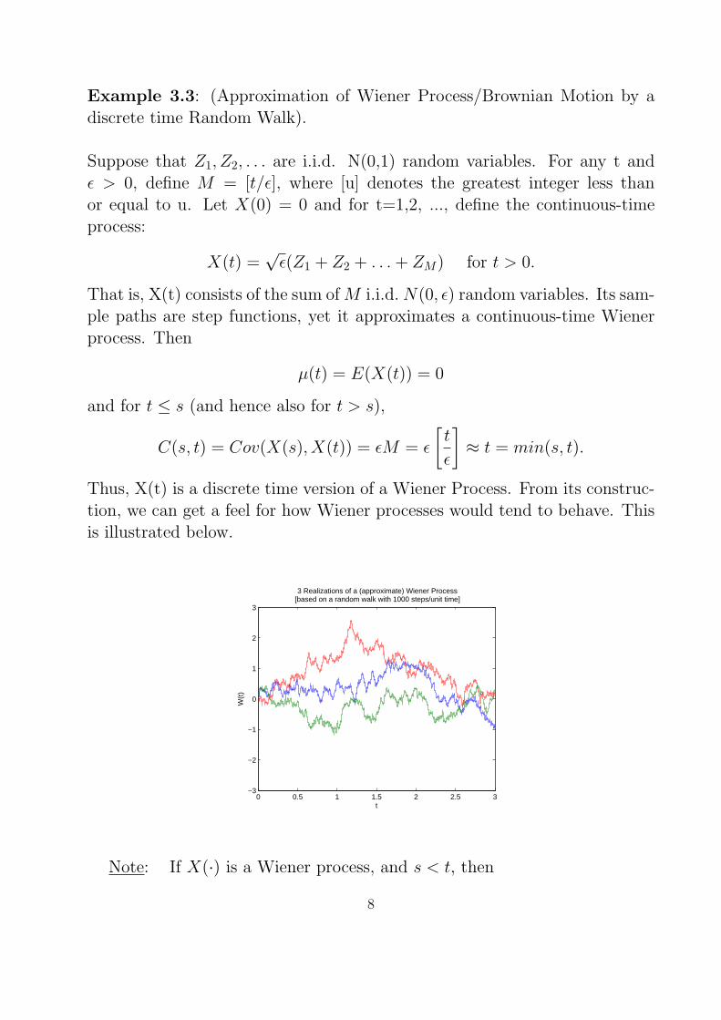
Example 3.3: (Approximation of Wiener Process/Brownian Motion by adiscrete time Random Walk).

Suppose that Z1, Z2, . . . are i.i.d. N(0,1) random variables. For any t andϵ > 0, define M = [t/ϵ], where [u] denotes the greatest integer less thanor equal to u. Let X(0) = 0 and for t=1,2, ..., define the continuous-timeprocess:

X(t) =√ϵ(Z1 + Z2 + . . .+ ZM) for t > 0.

That is, X(t) consists of the sum ofM i.i.d.N(0, ϵ) random variables. Its sam-ple paths are step functions, yet it approximates a continuous-time Wienerprocess. Then

µ(t) = E(X(t)) = 0

and for t ≤ s (and hence also for t > s),

C(s, t) = Cov(X(s), X(t)) = ϵM = ϵ

[t

ϵ

]≈ t = min(s, t).

Thus, X(t) is a discrete time version of a Wiener Process. From its construc-tion, we can get a feel for how Wiener processes would tend to behave. Thisis illustrated below.

0 0.5 1 1.5 2 2.5 3−3

−2

−1

0

1

2

3

t

W(t

)

3 Realizations of a (approximate) Wiener Process[based on a random walk with 1000 steps/unit time]

Note: If X(·) is a Wiener process, and s < t, then

8

Y (s, t)def= X(t)−X(s)

satisfies

(a) Y (s, t) ∼ N(0, t− s)

(b) Y (s1, t1) ⊥ Y (s2, t2)

for s1 < t1 ≤ s2 < t2.

That is, (a) tells us that displacements in a time interval have a distributionthat depends only on width of interval, and (b) tells us that the process X(·)has independent increments (Exercise 1).

Another functional of interest is the supremum Y of a Wiener Process X overa specific time interval; e.g.

Ydef= sup0≤t≤τ | X(t) | . (3.2)

One example where this arises is in forming confidence bands for a meanfunction; we return to this later in the course. It can be shown [see, forexample, Hall & Wellner (1980) and Schumacher (1984)] that for τ = 1 andfor any c > 0

P (Y ≤ c) =4

π

∞∑k=0

(−1)k

(2k + 1)e−π2(2k+1)2/8c2 .

Because of the complexity of this expression, these probabilities have beentabulated for various choices of c and time intervals (see Hall & Wellner andSchumacher).

Another functional of interest is the elapsed time, or passage time, until aprocess enters a specific state or takes a specific value. For example, whenmonitoring treatment differences over time in a clinical trial, suppose thatX(·) denotes some transformation of a test statistic. Then we might beinterested in the first time at which the test statistic attains some criticalvalue x; that is, in the distribution of the random variable

T (x)def= inft : X(t) ≥ x (3.3)

9

for some x > 0. In general, T(x) is referred to as the first passage time ofX(·) to the point x. Before developing this, we introduce the notion of stop-ping times.

Definition: Consider a stochastic process X(·) and let F(t) denote thesmallest σ-algebra with respect to which X(s) is measurable for each s ≤ t.Such σ-algebra exists (see Appendix A). Then a random variable T is calleda stopping time for X(·) if the event T ≤ t ∈ F(t) for every t (“at time t,it is known whether T ≤ t from the information on the process X”).

As we will see, the requirement reflected in this definition is necessary toensure that T (x) is a measurable random variable.

If the process X is continuous, T (x) is a stopping time:

T (x) ≤ t = ∪s≤t X(s) ≥ x

= ∩n∈N ∪q≤t,q∈Q

X(q) ≥ x− 1

n

,

where in both lines we use that X is continuous. The second equality holdssince X(s) ≥ x for some s if and only if for every n ∈ N there is q ∈ Q,q ≤ s such that X(q) ≥ x − 1

n . The last expression is in the σ-algebra be-cause countable unions (defining property) and countable intersections (seeExercises) are. Care is needed here: if X is not continuous, x could be thelimit lims↑tX(s) without X reaching x by t, or lims↓tX(s) could be greater orequal to x while x is not reached yet at t. Assuming continuity avoids theseissues. Convince yourself that assuming right continuity is necessary. Amongother things, this implies that for continuous processes, the first passage timeis a measurable random variable.

When the underlying process is a Wiener process, several useful and in-teresting results can be derived about first passage times. We discuss just afew here.

Theorem 3.1: Suppose W (·) is a Wiener process and that T (x) denotesthe resulting first passage time to the point x. Then the density function ofT (x) is given by

10

fT (x)(t) =| x |√2πt3

exp−x2

2t , (3.4)

for t ≥ 0. Note that because of the symmetry of a Wiener process, T(x)and T(-x) have the same distribution. One can show that this density arisesas that of Z−2, where Z has the N(0,x−2) distribution. The proof of Theo-rem 3.1 is given in Appendix B to this Unit.

Theorem 3.2: Suppose that W (·) is a Wiener process and define the ”sup”process M(·) by

M(t) = supW (s) : 0 ≤ s ≤ t .

Then M(t) has the same distribution as | W (t) |, and thus has density func-tion

fM(t)(m) = 21√2πt

exp(−m2

2t) for m ≥ 0.

The proof is given in Appendix B.

These results can be used to prove others, such as the following theoremabout the probability that a Wiener process crosses the zero axis during aspecified time interval. For the proof, see Grimmett & Stirzaker (2001).

Theorem 3.3: Suppose that W (·) is a Wiener process satisfying W(0)=0,and let 0 ≤ t0 < t1. Then

P (W (t) = 0 for some t ∈ (t0, t1)) =2

πcos−1

((t0/t1)

1/2).

This result illustrates some surprising properties of Wiener processes. Forexample, when t0 = 0, this says that the probability that a Wiener processequals zero in the interval (0, t) is 1 for every t > 0. This is not altogethersurprising when one thinks of a Wiener process as a limit of a random walk.

11

Indeed, there is an analogous theorem about a simple (symmetrically dis-tributed) random walk in discrete time ever crossing the horizontal axis.Continuing with this analogy (and with t0 = 0), it follows that the random

variable T (0)def= inft = 0 : W (t) = 0 is zero with probability 1. Further

investigation of this phenomenon shows that a Wiener process has infinitelymany zeros in any non-empty interval [0, t].

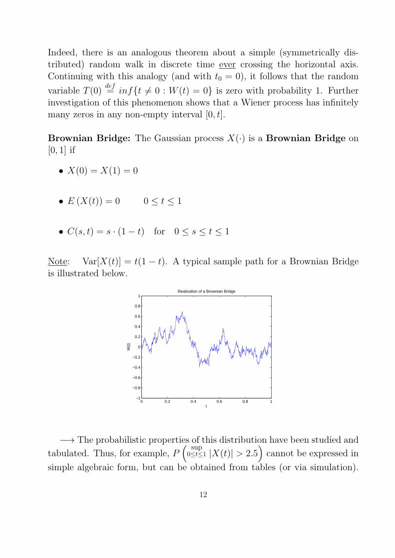
Brownian Bridge: The Gaussian process X(·) is a Brownian Bridge on[0, 1] if

• X(0) = X(1) = 0

• E (X(t)) = 0 0 ≤ t ≤ 1

• C(s, t) = s · (1− t) for 0 ≤ s ≤ t ≤ 1

Note: Var[X(t)] = t(1 − t). A typical sample path for a Brownian Bridgeis illustrated below.

0 0.2 0.4 0.6 0.8 1−1

−0.8

−0.6

−0.4

−0.2

0

0.2

0.4

0.6

0.8

1

t

W(t

)

Realization of a Brownian Bridge

−→ The probabilistic properties of this distribution have been studied and

tabulated. Thus, for example, P(

sup0≤t≤1 |X(t)| > 2.5

)cannot be expressed in

simple algebraic form, but can be obtained from tables (or via simulation).

12

We will discuss this further in a later unit.

It is easy to show (Exercise 3) that if W (·) is a Wiener process, then W0(·)defined by W (t)− t ·W (1) is a Brownian Bridge.

13

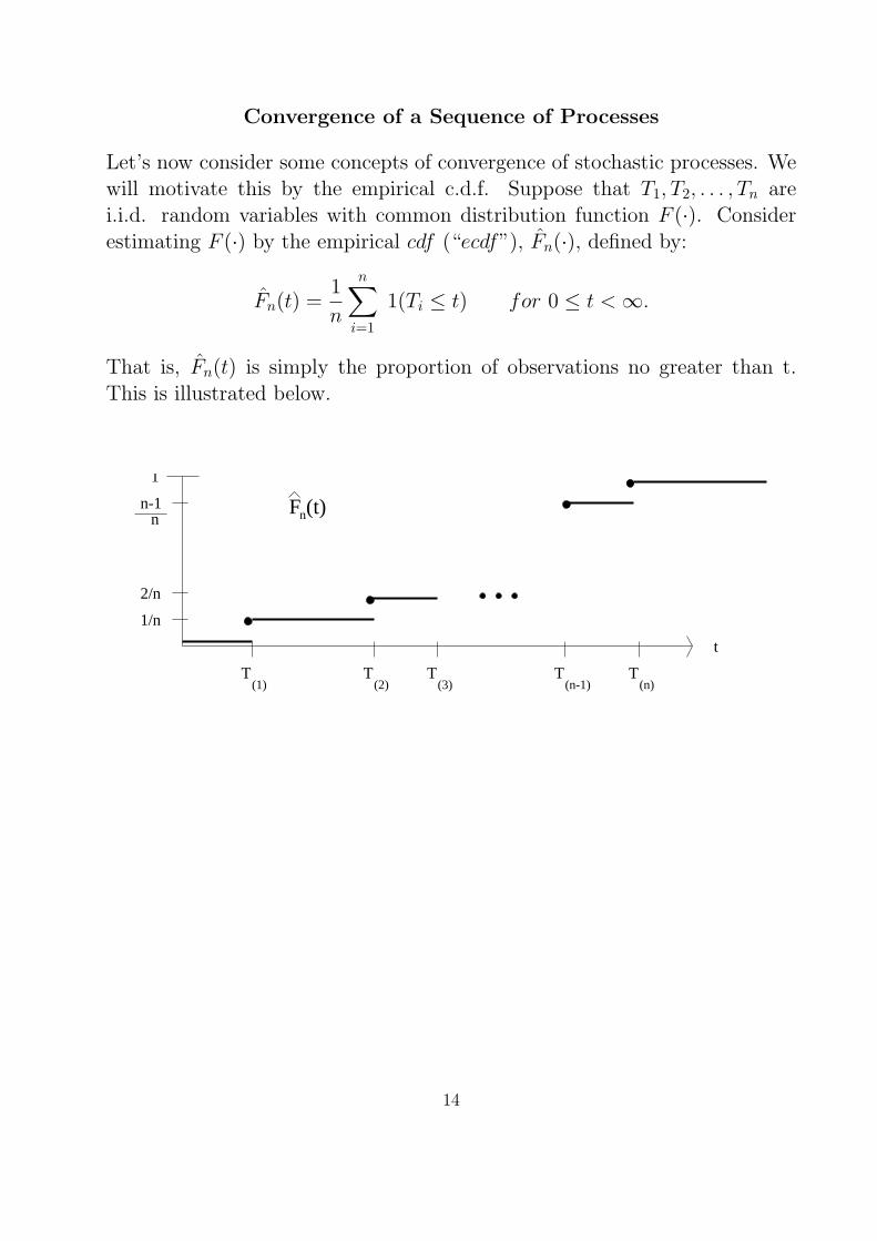
Convergence of a Sequence of Processes

Let’s now consider some concepts of convergence of stochastic processes. Wewill motivate this by the empirical c.d.f. Suppose that T1, T2, . . . , Tn arei.i.d. random variables with common distribution function F (·). Considerestimating F (·) by the empirical cdf (“ecdf”), Fn(·), defined by:

Fn(t) =1

n

n∑i=1

1(Ti ≤ t) for 0 ≤ t < ∞.

That is, Fn(t) is simply the proportion of observations no greater than t.This is illustrated below.

(2) (3) (n-1) (n)(1)

nF (t)

1

n-1n

2/n

1/n

T T T T T

t

14

Let’s examine some of its properties. First, fix t and note that if Zi = 1(Ti ≤t) for i=1,. . .,n, then Z1, Z2, · · · , Zn are i.i.d. Bernoulli(p), where p = F (t).Then we can write

Fn(t) =1

n

n∑i=1

Zi.

It follows that

• E[Fn(t)] = E[Zi] = F (t); i.e., Fn is unbiased

• Var[Fn(t)] =V (Zi)

n=

F (t) · [1− F (t)]

n

• Fn(t)P−→ F (t) as n → ∞ (by the WLLN)

•√nFn(t)− F (t)

L−→ N [0, F (t)[1− F (t)]]

as n → ∞ (by the ordinary CLT).

Thus, for example, an approximate 95% CI for p = F (t) is given by

Fn(t)± 1.96

√Fn(t)[1− Fn(t)]

n.

We have been focusing on the distribution of Fn(t) for the fixed t; i.e.,on the r.v. Zn = Fn(t). Later we will consider the entire stochasticprocess Fn(·). This requires us to define the concepts of ‘convergence’for stochastic processes.

15

Additional Reading and Discussion

The text by Grimmett and Stirzaker (2001) includes some useful results aboutstochastic processes, including some foundational considerations.

Sample Paths versus Finite Dimensional Distributions: The un-derlying phenomenon reflected in Example 3.1 leads to more general issuesin how to characterize and study the probabilistic properties of a stochasticprocess X(·). To examine this further, note that for any integer k and anyk times, say 0 ≤ t1 < t2 < · · · < tk < ∞, we can consider the usual distri-bution function of the k-vector (X(t1), X(t2), · · · , X(tk)). The set of all suchdistributions, for all integers k and all k-tuples (t1, t2, · · · , tk), is called the setof finite dimensional distributions (fdd) of X(·). Intuitively, one mightthink that knowledge of the fdd’s fully describes all probabilistic aspects ofa stochastic process. Alternatively, one could envision studying the proba-bilistic features of a process by studying the properties of its sample paths.Thus, we could:

(1) Study the properties of the sample paths X(·;ω) for every ω ∈ Ω; or

(2) Study the collection of finite dimensional distributions of X(·).

Because of the uncountably infinite number of random variables X(t) thatcomprise X(·), it turns out that the collection of fdd’s does not necessarilytell us everything of interest about the behavior of X(·). This is illustratedin the following example.

Example 3.4: Suppose that the random variable U is defined on the unitinterval probability space and has the Uniform(0,1) distribution. Considerthe 2 stochastic process, X(·) and Y (·), defined for 0 ≤ t ≤ 1 by X(t) = 0for all t and Y (t) = 1 when U = t and zero otherwise. Since P (U = t) = 0for every t, the processes X(·) and Y (·) have the same fdd’s; that is, for anyk, any 0 ≤ t1 < · · · < tk ≤ 1, and any x1, · · · , xk, we have that

P (X(t1) ≤ x1, · · · , X(tk) ≤ xk) = P (Y (t1) ≤ x1, · · · , Y (tk) ≤ xk) .

16

However,X(·) and Y (·) are clearly different processes. In particular, P (X(t) =0 for all t ) = 1 while P (Y (t) = 0 for all t ) = 0.

In general, we say that 2 stochastic processes are versions of one another ifthey have the same set of fdd’s. When our interest is in probabilistic featuresof a process that can be described in terms of its fdd’s, such as a patient’sblood sugar levels at monthly visits, non-identical processes that are versionsof one another will lead to the same probabilities. However, if we were inter-ested in a feature such as the elapsed time between states of a process, twoprocesses that are versions of one another may have different properties. Forexample, in Example 3.4, consider the time until each process first takes thevalue 1. The process X(·) never takes such a value while for the process Y (·),the time is just U .

The previous example illustrates that the fdd’s of a stochastic process do notnecessarily describe all of its probabilistic features. An underlying problemcausing this is that σ-algebras need not be closed under an uncountably in-finite number of intersections. If all events of interest could be described interms of a countably infinite number of unions or intersections of events inA, then we could avoid this problem. For example, suppose that the samplepaths of a stochastic process are continuous in t. Then since the rationalsare dense in R, knowledge of the values of each sample path X(·;ω) for allrational t would fully determine the sample path. Thus, any events describ-able by the process would be elements in the σ-algebra A. This suggests thatthe problems illustrated above can be avoided if we restricted ourselves toprocesses whose sample paths were continuous. This is further illustrated inthe following example.

Example 3.5: Consider the unit interval probability space and supposethat W (·) is a Wiener Process. Define the random variable S to be theelapsed time until W (·) first takes the value 1; that is,

S = inft : W (t) = 1 .

It follows that the event S > t can be expressed as

17

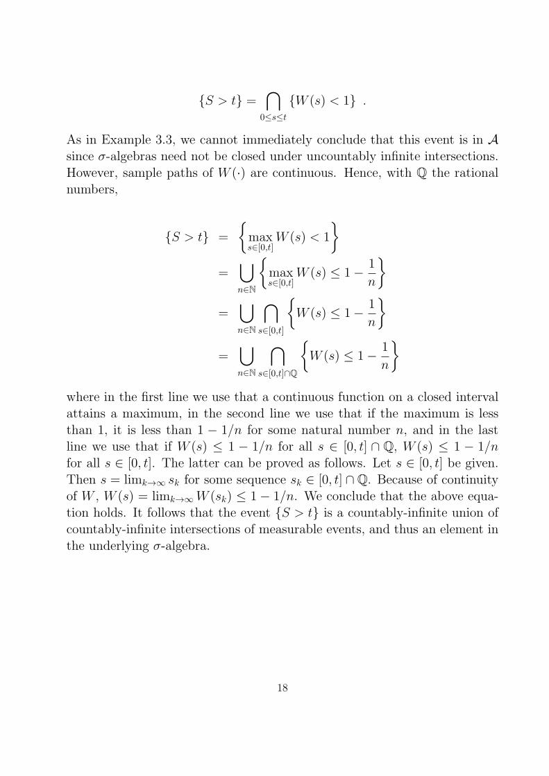
S > t =∩

0≤s≤t

W (s) < 1 .

As in Example 3.3, we cannot immediately conclude that this event is in Asince σ-algebras need not be closed under uncountably infinite intersections.However, sample paths of W (·) are continuous. Hence, with Q the rationalnumbers,

S > t =

maxs∈[0,t]

W (s) < 1

=

∪n∈N

maxs∈[0,t]

W (s) ≤ 1− 1

n

=

∪n∈N

∩s∈[0,t]

W (s) ≤ 1− 1

n

=

∪n∈N

∩s∈[0,t]∩Q

W (s) ≤ 1− 1

n

where in the first line we use that a continuous function on a closed intervalattains a maximum, in the second line we use that if the maximum is lessthan 1, it is less than 1 − 1/n for some natural number n, and in the lastline we use that if W (s) ≤ 1 − 1/n for all s ∈ [0, t] ∩ Q, W (s) ≤ 1 − 1/nfor all s ∈ [0, t]. The latter can be proved as follows. Let s ∈ [0, t] be given.Then s = limk→∞ sk for some sequence sk ∈ [0, t] ∩Q. Because of continuityof W , W (s) = limk→∞W (sk) ≤ 1− 1/n. We conclude that the above equa-tion holds. It follows that the event S > t is a countably-infinite union ofcountably-infinite intersections of measurable events, and thus an element inthe underlying σ-algebra.

18

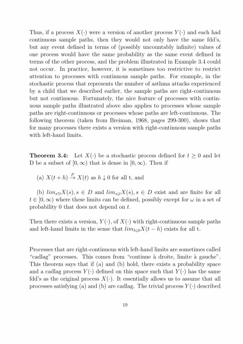
Thus, if a process X(·) were a version of another process Y (·) and each hadcontinuous sample paths, then they would not only have the same fdd’s,but any event defined in terms of (possibly uncountably infinite) values ofone process would have the same probability as the same event defined interms of the other process, and the problem illustrated in Example 3.4 couldnot occur. In practice, however, it is sometimes too restrictive to restrictattention to processes with continuous sample paths. For example, in thestochastic process that represents the number of asthma attacks experiencedby a child that we described earlier, the sample paths are right-continuousbut not continuous. Fortunately, the nice feature of processes with contin-uous sample paths illustrated above also applies to processes whose samplepaths are right-continuous or processes whose paths are left-continuous. Thefollowing theorem (taken from Breiman, 1968, pages 299-300), shows thatfor many processes there exists a version with right-continuous sample pathswith left-hand limits.

Theorem 3.4: Let X(·) be a stochastic process defined for t ≥ 0 and letD be a subset of [0,∞) that is dense in [0,∞). Then if

(a) X(t+ h)P→ X(t) as h ↓ 0 for all t, and

(b) lims↑tX(s), s ∈ D and lims↓tX(s), s ∈ D exist and are finite for allt ∈ [0,∞) where these limits can be defined, possibly except for ω in a set ofprobability 0 that does not depend on t.

Then there exists a version, Y (·), of X(·) with right-continuous sample pathsand left-hand limits in the sense that limh↓0X(t− h) exists for all t.

Processes that are right-continuous with left-hand limits are sometimes called“cadlag” processes. This comes from “continue a droite, limite a gauche”.This theorem says that if (a) and (b) hold, there exists a probability spaceand a cadlag process Y (·) defined on this space such that Y (·) has the samefdd’s as the original process X(·). It essentially allows us to assume that allprocesses satisfying (a) and (b) are cadlag. The trivial process Y (·) described

19

in Example 3.4 is seen to satisfy these conditions. Other processes, such asthe empirical c.d.f. Fn(·) are already cadlag. Yet others need not be, yet wewill later see that one can find a version that is cadlag or that has continuoussample paths. When we study Gaussian processes, we will usually restrictourselves to processes with continuous sample paths.

We conclude this discussion with one additional existence consideration. Weoften begin a discussion with something like ”Suppose that X(·) is a Gaus-sian process ....”. But how do we know that such processes exist? With arandom variable, say X ∼ F (·), this can be shown by simple construction.For example, with the unit interval probability space we can define the Uni-form[0,1] random variable U by U(ω) = ω and then define X = F−1(U). Isthere an analogy for stochastic processes? The answer is yes; for a formalproof see the text by Kingman & Taylor (1973) or the text by Grimmett &Stirzaker (2001). This can be seen heuristically by viewing a Wiener processW (·) as a limiting case of a simple random walk in discrete time. The samecan be done with other processes. For example, Brownian Bridge processes,say W0(·), can be constructed via Wiener processes by W0(t) = W (t)−tW (1)for 0 ≤ t ≤ 1.

20

Appendix A

Probability Spaces and Random Variables

1. An axiomatic treatment of probability starts with “outcomes” from arandom experiment. A random experiment refers to any repeatablemechanism that generates values in some set Ω, called the sample space.In case we observe only one survival time, the form of Ω could sim-ply be R. In case we observe n survival times, the form of Ω could beRn. When researching properties of estimators, we often consider sam-ple spaces on which a countable number of survival times are defined(n = 1, . . . ,∞), sometimes combined with, possibly even time depen-dent, covariates. The form of Ω is then more complex. Usually we donot bother about the form of Ω.

2. An event is a subset of the sample space. A probability is a functiondefined on a collection of events satisfying some axioms. We wouldlike to be able to form new events via operations like taking unions andcomplements of events and to compute the probability of the new events.It turns out that a theory of probability that is both useful and quitegeneral can be built by allowing countable operations. This entails usingσ-algebras as the collection of events, and countably additive measuresas the probabilities; see below.

3. A σ-algebra is a collection A of subsets of Ω satisfying some properties.Often, especially later in this course, the idea behind a σ-algebra is thatafter an experiment, some information on ω ∈ Ω is revealed: after theexperiment we know for all A ∈ A whether ω ∈ A or not. The definingproperties of a σ-algebra A are:

• ∅ ∈ A• Closed under complementation: A ∈ A ⇒ Ac ∈ A.

• Closed under countable unions: An ∈ A, n ∈ N ⇒ ∪n∈NAn ∈ A.

Sets in the σ-algebra are called measurable sets. An example of a σ-algebra on Ω = 1, 2, 3 is the collection of sets ∅, 1, 2, 3, and1, 2, 3. The meaning of this is that after the experiment, it is knownwhether ω = 1. Another example of a σ-algebra on Ω = 1, 2, 3 is the

21

collection of all subsets of 1, 2, 3. The meaning of this is that after theexperiment, it is known whether ω is 1, 2, or 3. This way, it is clear thatthe “richer” σ-algebra, containing more sets, reveals more informationon ω.

4. It can be shown (Exercise 4) that intersections of elements in the σ-algebra are also elements of the σ-algebra. This is also true for countableintersections.

5. A probability space is a sample space Ω along with a σ-algebra A definedon the sample space: (Ω,A).

6. A probability measure on a probability space (Ω,A) is a set functionP : A → [0, 1] satisfying:

• P (Ω) = 1

• Countable additivity: if An ∈ A, n ∈ N and An pairwise disjoint,then P (∪n∈NAn) =

∑n∈N P (An).

The σ-algebra here is important, since it turns out that it is not alwayspossible to meaningfully assign probabilities to all subsets of the samplespace; hence, not always all subsets of the sample space are events, ormembers of A.

7. So, after the experiment, we observe whether ω ∈ A for all A ∈ A, andbefore the experiment, there is a probability of ω ∈ A for all A ∈ A. Arepresents the information available due to the experiment.

8. A scalar random variable X on (Ω,A, P ) is a mapX from Ω to R which ismeasurable: for any x ∈ R, ω ∈ Ω : X(ω) ≤ x ∈ A. Or, equivalently,X−1 ((−∞, x]) ∈ A.

9. Thus, for a random variableX, after the experiment, it is known whetherX ≤ x, and before the experiment, there is a probability attached towhether or not X ≤ x.

10. It turns out that if X is a random variable on (Ω,A, P ), also, for everyx ∈ R:

• ω ∈ Ω : X(ω) ≥ x ∈ A

22

• ω ∈ Ω : X(ω) = x ∈ A• ω ∈ Ω : X(ω) < x ∈ A• ω ∈ Ω : X(ω) > x ∈ A.

Hence, these are all events, and their probabilities are well-defined.These properties follow from the properties of a σ-algebra. See alsoExercise 4.

11. Notice that the set of all subsets of Ω is a σ-algebra. For Ω = 1, 2, 3,this would be the collection of sets ∅, 1, 2, 3, 1, 2, 1, 3, 2, 3,and 1, 2, 3. Convince yourself that the intersection of σ-algebras isagain a σ-algebra. Hence, for any collection D of sets of Ω, there existsa smallest σ-algebra containing all sets in D (it is the intersection of allσ-algebras containing D). This is called the σ-algebra generated by D.For example, with Ω = 1, 2, 3, the σ-algebra generated by the set 1consists of the following sets: ∅, 1, 2, 3, 1, 2, 3. Again, this is theσ-algebra revealing information on whether or not ω = 1.

12. Note: although σ-algebras are defined through countable operations, theσ-algebra generated by a collection of sets is not necessarily obtained bycountable operations on the collection. (This is not easy to see).

13. The Borel σ-algebra B on [0, 1] is the σ-algebra generated by the intervals[0, x]: x ∈ [0, 1]. Not all subsets of [0, 1] are in the Borel σ-algebra.Convince yourself that points and intervals (open, closed, half open andhalf closed) are in the Borel σ-algebra.

14. Similarly, the Borel σ-algebra B on [0,∞) is the σ-algebra generated bythe intervals [0, x]: x ∈ [0,∞).

15. Some examples in this unit mention the unit interval probability space([0, 1] ,B, µ) with B the Borel σ-algebra and µ the Lebesgue measure.The Lebesgue measure assigns probability x to each interval [0, x]: x ∈[0, 1]. One can show that that leads to a unique probability measureon the probability space ([0, 1] ,B). Under the Lebesgue-measure, theprobability of ω falling in any interval in [0, 1] equals the length of thatinterval. This is true for open, closed, or half open and half closedintervals. Thus, all values in [0, 1] are equally likely. And if you considerω as a random variable, it has the uniform[0, 1]-distribution.

23

For more about random variables and σ-algebras we refer to the book “Prob-ability and Measure” by Billingsly (1995).

24

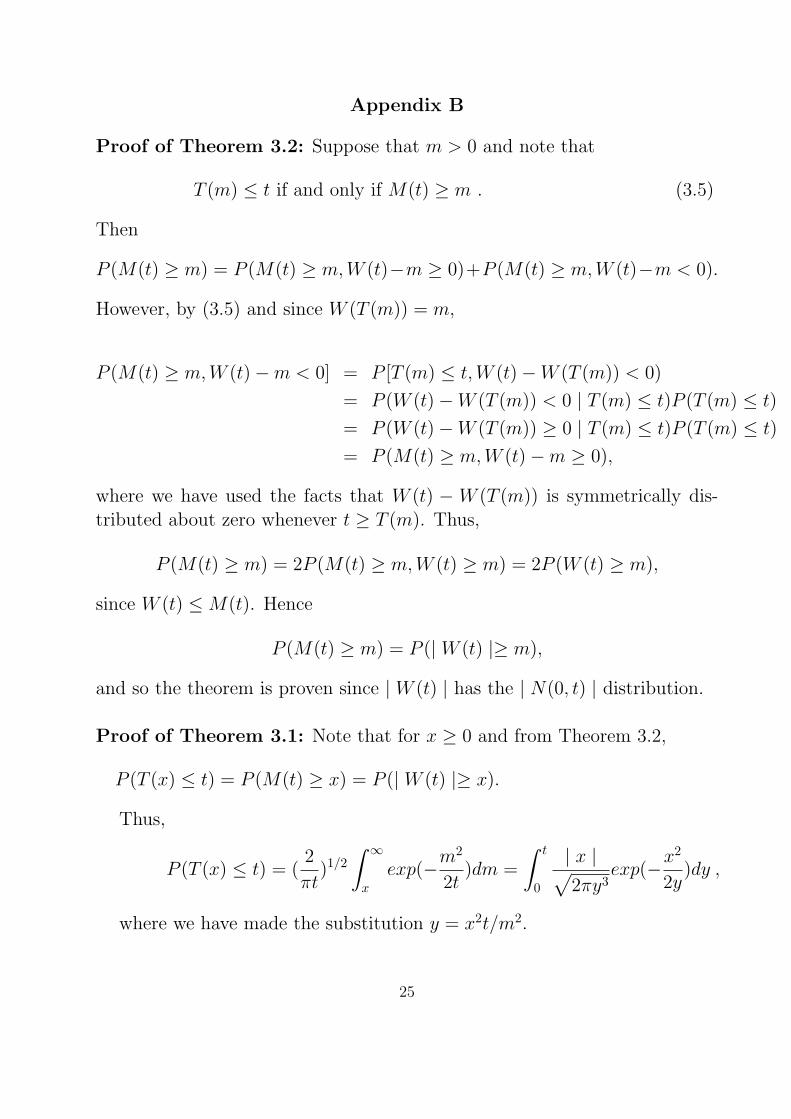
Appendix B

Proof of Theorem 3.2: Suppose that m > 0 and note that

T (m) ≤ t if and only if M(t) ≥ m . (3.5)

Then

P (M(t) ≥ m) = P (M(t) ≥ m,W (t)−m ≥ 0)+P (M(t) ≥ m,W (t)−m < 0).

However, by (3.5) and since W (T (m)) = m,

P (M(t) ≥ m,W (t)−m < 0] = P [T (m) ≤ t,W (t)−W (T (m)) < 0)

= P (W (t)−W (T (m)) < 0 | T (m) ≤ t)P (T (m) ≤ t)

= P (W (t)−W (T (m)) ≥ 0 | T (m) ≤ t)P (T (m) ≤ t)

= P (M(t) ≥ m,W (t)−m ≥ 0),

where we have used the facts that W (t) − W (T (m)) is symmetrically dis-tributed about zero whenever t ≥ T (m). Thus,

P (M(t) ≥ m) = 2P (M(t) ≥ m,W (t) ≥ m) = 2P (W (t) ≥ m),

since W (t) ≤ M(t). Hence

P (M(t) ≥ m) = P (| W (t) |≥ m),

and so the theorem is proven since | W (t) | has the | N(0, t) | distribution.

Proof of Theorem 3.1: Note that for x ≥ 0 and from Theorem 3.2,

P (T (x) ≤ t) = P (M(t) ≥ x) = P (| W (t) |≥ x).

Thus,

P (T (x) ≤ t) = (2

πt)1/2

∫ ∞

x

exp(−m2

2t)dm =

∫ t

0

| x |√2πy3

exp(−x2

2y)dy ,

where we have made the substitution y = x2t/m2.

25

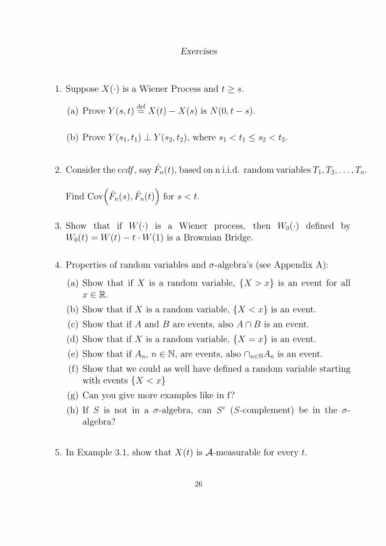
Exercises

1. Suppose X(·) is a Wiener Process and t ≥ s.

(a) Prove Y (s, t)def= X(t)−X(s) is N(0, t− s).

(b) Prove Y (s1, t1) ⊥ Y (s2, t2), where s1 < t1 ≤ s2 < t2.

2. Consider the ecdf , say Fn(t), based on n i.i.d. random variables T1, T2, . . . , Tn.

Find Cov(Fn(s), Fn(t)

)for s < t.

3. Show that if W (·) is a Wiener process, then W0(·) defined byW0(t) = W (t)− t ·W (1) is a Brownian Bridge.

4. Properties of random variables and σ-algebra’s (see Appendix A):

(a) Show that if X is a random variable, X > x is an event for allx ∈ R.

(b) Show that if X is a random variable, X < x is an event.

(c) Show that if A and B are events, also A ∩B is an event.

(d) Show that if X is a random variable, X = x is an event.

(e) Show that if An, n ∈ N, are events, also ∩n∈NAn is an event.

(f) Show that we could as well have defined a random variable startingwith events X < x

(g) Can you give more examples like in f?

(h) If S is not in a σ-algebra, can Sc (S-complement) be in the σ-algebra?

5. In Example 3.1, show that X(t) is A-measurable for every t.

26

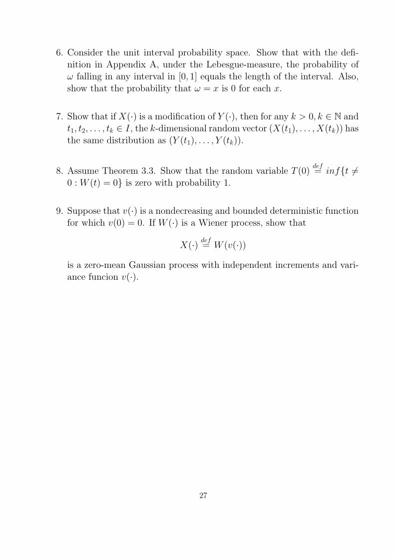
6. Consider the unit interval probability space. Show that with the defi-nition in Appendix A, under the Lebesgue-measure, the probability ofω falling in any interval in [0, 1] equals the length of the interval. Also,show that the probability that ω = x is 0 for each x.

7. Show that if X(·) is a modification of Y (·), then for any k > 0, k ∈ N andt1, t2, . . . , tk ∈ I, the k-dimensional random vector (X(t1), . . . , X(tk)) hasthe same distribution as (Y (t1), . . . , Y (tk)).

8. Assume Theorem 3.3. Show that the random variable T (0)def= inft =

0 : W (t) = 0 is zero with probability 1.

9. Suppose that v(·) is a nondecreasing and bounded deterministic functionfor which v(0) = 0. If W (·) is a Wiener process, show that

X(·) def= W (v(·))

is a zero-mean Gaussian process with independent increments and vari-ance funcion v(·).

27

References

Billingsley P. (1995). Probability and Measure, 3rd Edition, Wiley, NewYork.

Breiman (1968). Probability.

Cox DR & Miller HD (1965), Theory of Stochastic Processes, Methuen, Lon-don.

Fleming TR & Harrington DP (1991). Counting Processes and Survival Anal-ysis, Wiley, NY.

Grimmett G & Stirzaker D (2001). Probability and Random Processes, 3rdEdition, Oxford University Press, Oxford, UK.

Hall & Wellner (1980). Biometrika 67:133-144.

Kingman JFC & Taylor SC (1973). Introduction to Measure and Probability,Cambridge University Press.

Schumacher (1984). Intl. Statis. Review 52:263-281)

28