6.801/6.866: Machine Vision Fall 2020

Lecture Notes

Professor Berthold Horn, Ryan Sander, Tadayuki YoshitakeDepartment of Electrical Engineering and Computer Science

Massachusetts Institute of Technology

Contents

1 Lecture 2: Image Formatio, Perspective Projection, Time Derivative, Motion Field 81.1 Motion from Perspective Projection, and FOE . . . . . . . . . . . . . . . . . . . . . . . . . . . . . . . . . . . . . 81.2 Brightness and Motion . . . . . . . . . . . . . . . . . . . . . . . . . . . . . . . . . . . . . . . . . . . . . . . . . . . 10

1.2.1 1D Case . . . . . . . . . . . . . . . . . . . . . . . . . . . . . . . . . . . . . . . . . . . . . . . . . . . . . . . 101.2.2 2D Case . . . . . . . . . . . . . . . . . . . . . . . . . . . . . . . . . . . . . . . . . . . . . . . . . . . . . . . 11

2 Lecture 3: Time to Contact, Focus of Expansion, Direct Motion Vision Methods, Noise Gain 122.1 Noise Gain . . . . . . . . . . . . . . . . . . . . . . . . . . . . . . . . . . . . . . . . . . . . . . . . . . . . . . . . . 122.2 Forward and Inverse Problems of Machine Vision . . . . . . . . . . . . . . . . . . . . . . . . . . . . . . . . . . . . 13

2.2.1 Scalar Case . . . . . . . . . . . . . . . . . . . . . . . . . . . . . . . . . . . . . . . . . . . . . . . . . . . . . 132.2.2 Vector Case . . . . . . . . . . . . . . . . . . . . . . . . . . . . . . . . . . . . . . . . . . . . . . . . . . . . . 13

2.3 Review from Lecture 2 . . . . . . . . . . . . . . . . . . . . . . . . . . . . . . . . . . . . . . . . . . . . . . . . . . . 142.3.1 Two-Pixel Motion Estimation, Vector Form . . . . . . . . . . . . . . . . . . . . . . . . . . . . . . . . . . . 142.3.2 Constant Brightness Assumption, and Motion Equation Derivation . . . . . . . . . . . . . . . . . . . . . . 142.3.3 Optical Mouse Problem . . . . . . . . . . . . . . . . . . . . . . . . . . . . . . . . . . . . . . . . . . . . . . 152.3.4 Perspective Projection . . . . . . . . . . . . . . . . . . . . . . . . . . . . . . . . . . . . . . . . . . . . . . . 15

2.4 Time to Contact (TTC) . . . . . . . . . . . . . . . . . . . . . . . . . . . . . . . . . . . . . . . . . . . . . . . . . . 15

3 Lecture 4: Fixed Optical Flow, Optical Mouse, Constant Brightness Assumption, Closed Form Solution 183.1 Review . . . . . . . . . . . . . . . . . . . . . . . . . . . . . . . . . . . . . . . . . . . . . . . . . . . . . . . . . . . . 18

3.1.1 Constant Brightness Assumption Review with Generalized Isophotes . . . . . . . . . . . . . . . . . . . . . 193.1.2 Time to Contact (TTC) Review . . . . . . . . . . . . . . . . . . . . . . . . . . . . . . . . . . . . . . . . . 19

3.2 Increasing Generality of TTC Problems . . . . . . . . . . . . . . . . . . . . . . . . . . . . . . . . . . . . . . . . . 203.3 Multiscale and TTC . . . . . . . . . . . . . . . . . . . . . . . . . . . . . . . . . . . . . . . . . . . . . . . . . . . . 20

3.3.1 Aliasing and Nyquist’s Sampling Theorem . . . . . . . . . . . . . . . . . . . . . . . . . . . . . . . . . . . . 213.3.2 Applications of TTC . . . . . . . . . . . . . . . . . . . . . . . . . . . . . . . . . . . . . . . . . . . . . . . . 21

3.4 Optical Flow . . . . . . . . . . . . . . . . . . . . . . . . . . . . . . . . . . . . . . . . . . . . . . . . . . . . . . . . 223.5 Vanishing Points (Perspective Projection) . . . . . . . . . . . . . . . . . . . . . . . . . . . . . . . . . . . . . . . . 22

3.5.1 Applications of Vanishing Points . . . . . . . . . . . . . . . . . . . . . . . . . . . . . . . . . . . . . . . . . 223.6 Calibration Objects . . . . . . . . . . . . . . . . . . . . . . . . . . . . . . . . . . . . . . . . . . . . . . . . . . . . 23

3.6.1 Spheres . . . . . . . . . . . . . . . . . . . . . . . . . . . . . . . . . . . . . . . . . . . . . . . . . . . . . . . 233.6.2 Cube . . . . . . . . . . . . . . . . . . . . . . . . . . . . . . . . . . . . . . . . . . . . . . . . . . . . . . . . . 23

3.7 Additional Topics . . . . . . . . . . . . . . . . . . . . . . . . . . . . . . . . . . . . . . . . . . . . . . . . . . . . . . 233.7.1 Generalization: Fixed Flow . . . . . . . . . . . . . . . . . . . . . . . . . . . . . . . . . . . . . . . . . . . . 243.7.2 Generalization: Time to Contact (for U = 0, V = 0, ω 6= 0) . . . . . . . . . . . . . . . . . . . . . . . . . . . 24

4 Lecture 5: TTC and FOR Montivision Demos, Vanishing Point, Use of VPs in Camera Calibration 254.1 Robust Estimation and Sampling . . . . . . . . . . . . . . . . . . . . . . . . . . . . . . . . . . . . . . . . . . . . . 26

4.1.1 Line Intersection Least-Squares . . . . . . . . . . . . . . . . . . . . . . . . . . . . . . . . . . . . . . . . . . 264.1.2 Dealing with Outliers . . . . . . . . . . . . . . . . . . . . . . . . . . . . . . . . . . . . . . . . . . . . . . . 264.1.3 Reprojection and Rectification . . . . . . . . . . . . . . . . . . . . . . . . . . . . . . . . . . . . . . . . . . 264.1.4 Resampling . . . . . . . . . . . . . . . . . . . . . . . . . . . . . . . . . . . . . . . . . . . . . . . . . . . . . 26

4.2 Magnification with TTC . . . . . . . . . . . . . . . . . . . . . . . . . . . . . . . . . . . . . . . . . . . . . . . . . . 274.2.1 Perspective Projection and Vanishing Points . . . . . . . . . . . . . . . . . . . . . . . . . . . . . . . . . . 274.2.2 Lines in 2D and 3D . . . . . . . . . . . . . . . . . . . . . . . . . . . . . . . . . . . . . . . . . . . . . . . . 284.2.3 Application: Multilateration (MLAT) . . . . . . . . . . . . . . . . . . . . . . . . . . . . . . . . . . . . . . 284.2.4 Application: Understand Orientation of Camera w.r.t. World . . . . . . . . . . . . . . . . . . . . . . . . . 29

4.3 Brightness . . . . . . . . . . . . . . . . . . . . . . . . . . . . . . . . . . . . . . . . . . . . . . . . . . . . . . . . . . 304.3.1 What if We Can’t use Multiple Orientations? . . . . . . . . . . . . . . . . . . . . . . . . . . . . . . . . . . 31

4.4 References . . . . . . . . . . . . . . . . . . . . . . . . . . . . . . . . . . . . . . . . . . . . . . . . . . . . . . . . . . 32

5 Lecture 6: Photometric Stereo, Noise Gain, Error Amplification, Eigenvalues and Eigenvectors Review 325.1 Applications of Linear Algebra to Motion Estimation/Noise Gain . . . . . . . . . . . . . . . . . . . . . . . . . . . 32

5.1.1 Application Revisited: Photometric Stereo . . . . . . . . . . . . . . . . . . . . . . . . . . . . . . . . . . . . 325.2 Lambertian Objects and Brightness . . . . . . . . . . . . . . . . . . . . . . . . . . . . . . . . . . . . . . . . . . . . 33

5.2.1 Surface Orientation . . . . . . . . . . . . . . . . . . . . . . . . . . . . . . . . . . . . . . . . . . . . . . . . 345.2.2 Surface Orientation Isophotes/Reflectance Maps for Lambertian Surfaces . . . . . . . . . . . . . . . . . . 34

5.3 References . . . . . . . . . . . . . . . . . . . . . . . . . . . . . . . . . . . . . . . . . . . . . . . . . . . . . . . . . . 35

1

6 Lecture 7: Gradient Space, Reflectance Map, Image Irradiance Equation, Gnomonic Projection 356.1 Surface Orientation Estimation (Cont.) & Reflectance Maps . . . . . . . . . . . . . . . . . . . . . . . . . . . . . . 35

6.1.1 Forward and Inverse Problems . . . . . . . . . . . . . . . . . . . . . . . . . . . . . . . . . . . . . . . . . . 356.1.2 Reflectance Map Example: Determining the Surface Normals of a Sphere . . . . . . . . . . . . . . . . . . 366.1.3 Computational Photometric Stereo . . . . . . . . . . . . . . . . . . . . . . . . . . . . . . . . . . . . . . . . 36

6.2 Photometry & Radiometry . . . . . . . . . . . . . . . . . . . . . . . . . . . . . . . . . . . . . . . . . . . . . . . . 366.3 Lenses . . . . . . . . . . . . . . . . . . . . . . . . . . . . . . . . . . . . . . . . . . . . . . . . . . . . . . . . . . . . 37

6.3.1 Thin Lenses - Introduction and Rules . . . . . . . . . . . . . . . . . . . . . . . . . . . . . . . . . . . . . . 376.3.2 Putting it All Together: Image Irradiance from Object Irradiance . . . . . . . . . . . . . . . . . . . . . . . 386.3.3 BRDF: Bidirectional Reflectance Distribution Function . . . . . . . . . . . . . . . . . . . . . . . . . . . . 386.3.4 Helmholtz Reciprocity . . . . . . . . . . . . . . . . . . . . . . . . . . . . . . . . . . . . . . . . . . . . . . . 39

6.4 References . . . . . . . . . . . . . . . . . . . . . . . . . . . . . . . . . . . . . . . . . . . . . . . . . . . . . . . . . . 39

7 Lecture 8: Shape from Shading, Special Cases, Lunar Surface, Scanning Electron Microscope, Green’sTheorem in Photometric Stereo 397.1 Review of Photometric and Radiometric Concepts . . . . . . . . . . . . . . . . . . . . . . . . . . . . . . . . . . . 407.2 Ideal Lambertian Surfaces . . . . . . . . . . . . . . . . . . . . . . . . . . . . . . . . . . . . . . . . . . . . . . . . . 40

7.2.1 Foreshortening Effects in Lambertian Surfaces . . . . . . . . . . . . . . . . . . . . . . . . . . . . . . . . . 417.2.2 Example: Distant Lambertian Point Source . . . . . . . . . . . . . . . . . . . . . . . . . . . . . . . . . . . 41

7.3 Hapke Surfaces . . . . . . . . . . . . . . . . . . . . . . . . . . . . . . . . . . . . . . . . . . . . . . . . . . . . . . . 417.3.1 Example Application: Imaging the Lunar Surface . . . . . . . . . . . . . . . . . . . . . . . . . . . . . . . . 427.3.2 Surface Orientation and Reflectance Maps of Hapke Surfaces . . . . . . . . . . . . . . . . . . . . . . . . . 437.3.3 Rotated (p′, q′) Coordinate Systems for Brightness Measurements . . . . . . . . . . . . . . . . . . . . . . . 43

7.4 “Thick” & Telecentric Lenses . . . . . . . . . . . . . . . . . . . . . . . . . . . . . . . . . . . . . . . . . . . . . . . 447.4.1 “Thick” Lenses . . . . . . . . . . . . . . . . . . . . . . . . . . . . . . . . . . . . . . . . . . . . . . . . . . . 447.4.2 Telecentric Lenses . . . . . . . . . . . . . . . . . . . . . . . . . . . . . . . . . . . . . . . . . . . . . . . . . 44

7.5 References . . . . . . . . . . . . . . . . . . . . . . . . . . . . . . . . . . . . . . . . . . . . . . . . . . . . . . . . . . 45

8 Lecture 9: Shape from Shading, General Case - From First Order Nonlinear PDE to Five ODEs 458.1 Example Applications: Transmission and Scanning Electron Microscopes (TEMs and SEMs, respectively) . . . . 468.2 Shape from Shading: Needle Diagram to Shape . . . . . . . . . . . . . . . . . . . . . . . . . . . . . . . . . . . . . 46

8.2.1 Derivation with Taylor Series Expansion . . . . . . . . . . . . . . . . . . . . . . . . . . . . . . . . . . . . . 478.2.2 Derivation with Green’s Theorem . . . . . . . . . . . . . . . . . . . . . . . . . . . . . . . . . . . . . . . . . 47

8.3 Shape with Discrete Optimization . . . . . . . . . . . . . . . . . . . . . . . . . . . . . . . . . . . . . . . . . . . . 488.3.1 “Computational Molecules” . . . . . . . . . . . . . . . . . . . . . . . . . . . . . . . . . . . . . . . . . . . . 498.3.2 Iterative Optimization Approach . . . . . . . . . . . . . . . . . . . . . . . . . . . . . . . . . . . . . . . . . 498.3.3 Reconstructing a Surface From a Single Image . . . . . . . . . . . . . . . . . . . . . . . . . . . . . . . . . 50

8.4 References . . . . . . . . . . . . . . . . . . . . . . . . . . . . . . . . . . . . . . . . . . . . . . . . . . . . . . . . . . 51

9 Lecture 10: Characteristic Strip Expansion, Shape from Shading, Iterative Solutions 519.1 Review: Where We Are and Shape From Shading . . . . . . . . . . . . . . . . . . . . . . . . . . . . . . . . . . . . 519.2 General Case . . . . . . . . . . . . . . . . . . . . . . . . . . . . . . . . . . . . . . . . . . . . . . . . . . . . . . . . 52

9.2.1 Reducing General Form SfS for Hapke Surfaces . . . . . . . . . . . . . . . . . . . . . . . . . . . . . . . . . 549.2.2 Applying General Form SfS to SEMs . . . . . . . . . . . . . . . . . . . . . . . . . . . . . . . . . . . . . . . 55

9.3 Base Characteristics . . . . . . . . . . . . . . . . . . . . . . . . . . . . . . . . . . . . . . . . . . . . . . . . . . . . 559.4 Analyzing “Speed” . . . . . . . . . . . . . . . . . . . . . . . . . . . . . . . . . . . . . . . . . . . . . . . . . . . . . 559.5 Generating an Initial Curve . . . . . . . . . . . . . . . . . . . . . . . . . . . . . . . . . . . . . . . . . . . . . . . . 56

9.5.1 Using Edge Points to Autogenerate an Initial Curve . . . . . . . . . . . . . . . . . . . . . . . . . . . . . . 569.5.2 Using Stationary Points to Autogenerate an Initial Curve . . . . . . . . . . . . . . . . . . . . . . . . . . . 569.5.3 Example . . . . . . . . . . . . . . . . . . . . . . . . . . . . . . . . . . . . . . . . . . . . . . . . . . . . . . . 57

9.6 References . . . . . . . . . . . . . . . . . . . . . . . . . . . . . . . . . . . . . . . . . . . . . . . . . . . . . . . . . . 58

10 Lecture 11: Edge Detection, Subpixel Position, CORDIC, Line Detection, (US 6,408,109) 5810.1 Background on Patents . . . . . . . . . . . . . . . . . . . . . . . . . . . . . . . . . . . . . . . . . . . . . . . . . . 5810.2 Patent Case Study: Detecting Sub-Pixel Location of Edges in a Digital Image . . . . . . . . . . . . . . . . . . . . 59

10.2.1 High-Level Overview of Edge Detection System . . . . . . . . . . . . . . . . . . . . . . . . . . . . . . . . . 6010.3 Edges & Edge Detection . . . . . . . . . . . . . . . . . . . . . . . . . . . . . . . . . . . . . . . . . . . . . . . . . . 61

10.3.1 Finding a Suitable Brightness Function for Edge Detection . . . . . . . . . . . . . . . . . . . . . . . . . . 6110.3.2 Brightness Gradient Estimation . . . . . . . . . . . . . . . . . . . . . . . . . . . . . . . . . . . . . . . . . . 62

2

10.4 References . . . . . . . . . . . . . . . . . . . . . . . . . . . . . . . . . . . . . . . . . . . . . . . . . . . . . . . . . . 64

11 Lecture 12: Blob analysis, Binary Image Processing, Use of Green’s Theorem, Derivative and Integral asConvolutions 6411.1 Types of Intellectual Property . . . . . . . . . . . . . . . . . . . . . . . . . . . . . . . . . . . . . . . . . . . . . . . 6411.2 Edge Detection Patent Methodologies . . . . . . . . . . . . . . . . . . . . . . . . . . . . . . . . . . . . . . . . . . 65

11.2.1 Finding Edge with Derivatives . . . . . . . . . . . . . . . . . . . . . . . . . . . . . . . . . . . . . . . . . . 6511.2.2 More on “Stencils”/Computational Molecules . . . . . . . . . . . . . . . . . . . . . . . . . . . . . . . . . . 6711.2.3 Mixed Partial Derivatives in 2D . . . . . . . . . . . . . . . . . . . . . . . . . . . . . . . . . . . . . . . . . . 6911.2.4 Laplacian Estimators in 2D . . . . . . . . . . . . . . . . . . . . . . . . . . . . . . . . . . . . . . . . . . . . 6911.2.5 Non-Maximum Suppression . . . . . . . . . . . . . . . . . . . . . . . . . . . . . . . . . . . . . . . . . . . . 7011.2.6 Plane Position . . . . . . . . . . . . . . . . . . . . . . . . . . . . . . . . . . . . . . . . . . . . . . . . . . . 7011.2.7 Bias Compensation . . . . . . . . . . . . . . . . . . . . . . . . . . . . . . . . . . . . . . . . . . . . . . . . . 7011.2.8 Edge Transition and Defocusing Compensation . . . . . . . . . . . . . . . . . . . . . . . . . . . . . . . . . 7011.2.9 Multiscale . . . . . . . . . . . . . . . . . . . . . . . . . . . . . . . . . . . . . . . . . . . . . . . . . . . . . . 7111.2.10 Effect on Image Edge . . . . . . . . . . . . . . . . . . . . . . . . . . . . . . . . . . . . . . . . . . . . . . . 7111.2.11 Addressing Quantization of Gradient Directions . . . . . . . . . . . . . . . . . . . . . . . . . . . . . . . . . 7111.2.12 CORDIC . . . . . . . . . . . . . . . . . . . . . . . . . . . . . . . . . . . . . . . . . . . . . . . . . . . . . . 72

11.3 References . . . . . . . . . . . . . . . . . . . . . . . . . . . . . . . . . . . . . . . . . . . . . . . . . . . . . . . . . . 72

12 Lecture 13: Object detection, Recognition and Pose Determination, PatQuick (US 7,016,539) 7212.1 Motivation & Preliminaries for Object Detection/Pose Estimation . . . . . . . . . . . . . . . . . . . . . . . . . . 72

12.1.1 “Blob Analysis”/”Binary Image Processing” . . . . . . . . . . . . . . . . . . . . . . . . . . . . . . . . . . . 7312.1.2 Binary Template . . . . . . . . . . . . . . . . . . . . . . . . . . . . . . . . . . . . . . . . . . . . . . . . . . 7312.1.3 Normalized Correlation . . . . . . . . . . . . . . . . . . . . . . . . . . . . . . . . . . . . . . . . . . . . . . 73

12.2 Patent 7,016,539: Method for Fast, Robust, Multidimensional Pattern Recognition . . . . . . . . . . . . . . . . . 7512.2.1 Patent Overview . . . . . . . . . . . . . . . . . . . . . . . . . . . . . . . . . . . . . . . . . . . . . . . . . . 7512.2.2 High-level Steps of Algorithm . . . . . . . . . . . . . . . . . . . . . . . . . . . . . . . . . . . . . . . . . . . 7512.2.3 Framework as Programming Objects . . . . . . . . . . . . . . . . . . . . . . . . . . . . . . . . . . . . . . . 7612.2.4 Other Considerations for this Framework . . . . . . . . . . . . . . . . . . . . . . . . . . . . . . . . . . . . 77

12.3 References . . . . . . . . . . . . . . . . . . . . . . . . . . . . . . . . . . . . . . . . . . . . . . . . . . . . . . . . . . 77

13 Lecture 14: Inspection in PatQuick, Hough Transform, Homography, Position Determination, Multi-Scale 7713.1 Review of “PatQuick” . . . . . . . . . . . . . . . . . . . . . . . . . . . . . . . . . . . . . . . . . . . . . . . . . . . 77

13.1.1 Scoring Functions . . . . . . . . . . . . . . . . . . . . . . . . . . . . . . . . . . . . . . . . . . . . . . . . . 7813.1.2 Additional System Considerations . . . . . . . . . . . . . . . . . . . . . . . . . . . . . . . . . . . . . . . . 7913.1.3 Another Application of “PatQuick”: Machine Inspection . . . . . . . . . . . . . . . . . . . . . . . . . . . . 80

13.2 Intro to Homography and Relative Poses . . . . . . . . . . . . . . . . . . . . . . . . . . . . . . . . . . . . . . . . . 8013.2.1 How many degrees of freedom . . . . . . . . . . . . . . . . . . . . . . . . . . . . . . . . . . . . . . . . . . . 81

13.3 Hough Transforms . . . . . . . . . . . . . . . . . . . . . . . . . . . . . . . . . . . . . . . . . . . . . . . . . . . . . 8113.3.1 Hough Transforms with Lines . . . . . . . . . . . . . . . . . . . . . . . . . . . . . . . . . . . . . . . . . . . 8113.3.2 Hough Transforms with Circles . . . . . . . . . . . . . . . . . . . . . . . . . . . . . . . . . . . . . . . . . . 8213.3.3 Hough Transforms with Searching for Center Position and Radius . . . . . . . . . . . . . . . . . . . . . . 82

13.4 Sampling/Subsampling/Multiscale . . . . . . . . . . . . . . . . . . . . . . . . . . . . . . . . . . . . . . . . . . . . 83

14 Lecture 15: Alignment, recognition in PatMAx, distance field, filtering and sub-sampling (US 7,065,262) 8314.1 PatMAx . . . . . . . . . . . . . . . . . . . . . . . . . . . . . . . . . . . . . . . . . . . . . . . . . . . . . . . . . . . 83

14.1.1 Overview . . . . . . . . . . . . . . . . . . . . . . . . . . . . . . . . . . . . . . . . . . . . . . . . . . . . . . 8314.1.2 Training PatMAx . . . . . . . . . . . . . . . . . . . . . . . . . . . . . . . . . . . . . . . . . . . . . . . . . . 8414.1.3 Estimating Other Pixels . . . . . . . . . . . . . . . . . . . . . . . . . . . . . . . . . . . . . . . . . . . . . . 8514.1.4 Attraction Module . . . . . . . . . . . . . . . . . . . . . . . . . . . . . . . . . . . . . . . . . . . . . . . . . 8514.1.5 PatMAx Claims . . . . . . . . . . . . . . . . . . . . . . . . . . . . . . . . . . . . . . . . . . . . . . . . . . 8614.1.6 Comparing PatMAx to PatQuick . . . . . . . . . . . . . . . . . . . . . . . . . . . . . . . . . . . . . . . . . 8714.1.7 Field Generation for PatMAx . . . . . . . . . . . . . . . . . . . . . . . . . . . . . . . . . . . . . . . . . . . 87

14.2 Finding Distance to Lines . . . . . . . . . . . . . . . . . . . . . . . . . . . . . . . . . . . . . . . . . . . . . . . . . 8814.3 Fast Convolutions Through Sparsity . . . . . . . . . . . . . . . . . . . . . . . . . . . . . . . . . . . . . . . . . . . 89

14.3.1 System Overview . . . . . . . . . . . . . . . . . . . . . . . . . . . . . . . . . . . . . . . . . . . . . . . . . . 9014.3.2 Integration and Differentiation as Convolutions . . . . . . . . . . . . . . . . . . . . . . . . . . . . . . . . . 9114.3.3 Sparse Convolution as Compression . . . . . . . . . . . . . . . . . . . . . . . . . . . . . . . . . . . . . . . 91

3

14.3.4 Effects on Scaling . . . . . . . . . . . . . . . . . . . . . . . . . . . . . . . . . . . . . . . . . . . . . . . . . . 9114.3.5 Filtering (For Multiscale): Anti-Aliasing . . . . . . . . . . . . . . . . . . . . . . . . . . . . . . . . . . . . . 9214.3.6 Extending Filtering to 2D and An Open Research Problem . . . . . . . . . . . . . . . . . . . . . . . . . . 92

15 Lecture 16: Fast Convolution, Low Pass Filter Approximations, Integral Images, (US 6,457,032) 9215.1 Sampling and Aliasing . . . . . . . . . . . . . . . . . . . . . . . . . . . . . . . . . . . . . . . . . . . . . . . . . . . 92

15.1.1 Nyquist Sampling Theorem . . . . . . . . . . . . . . . . . . . . . . . . . . . . . . . . . . . . . . . . . . . . 9215.1.2 Aliasing . . . . . . . . . . . . . . . . . . . . . . . . . . . . . . . . . . . . . . . . . . . . . . . . . . . . . . . 9415.1.3 How Can We Mitigate Aliasing? . . . . . . . . . . . . . . . . . . . . . . . . . . . . . . . . . . . . . . . . . 95

15.2 Integral Image . . . . . . . . . . . . . . . . . . . . . . . . . . . . . . . . . . . . . . . . . . . . . . . . . . . . . . . 9515.2.1 Integral Images in 1D . . . . . . . . . . . . . . . . . . . . . . . . . . . . . . . . . . . . . . . . . . . . . . . 9515.2.2 Integral Images in 2D . . . . . . . . . . . . . . . . . . . . . . . . . . . . . . . . . . . . . . . . . . . . . . . 95

15.3 Fourier Analysis of Block Averaging . . . . . . . . . . . . . . . . . . . . . . . . . . . . . . . . . . . . . . . . . . . 9615.4 Repeated Block Averaging . . . . . . . . . . . . . . . . . . . . . . . . . . . . . . . . . . . . . . . . . . . . . . . . . 99

15.4.1 Warping Effects and Numerical Fourier Transforms: FFT and DFT . . . . . . . . . . . . . . . . . . . . . 10115.5 Impulses and Convolution . . . . . . . . . . . . . . . . . . . . . . . . . . . . . . . . . . . . . . . . . . . . . . . . . 102

15.5.1 Properties of Delta Functions . . . . . . . . . . . . . . . . . . . . . . . . . . . . . . . . . . . . . . . . . . . 10215.5.2 Combinations of Impulses . . . . . . . . . . . . . . . . . . . . . . . . . . . . . . . . . . . . . . . . . . . . . 10215.5.3 Convolution Review . . . . . . . . . . . . . . . . . . . . . . . . . . . . . . . . . . . . . . . . . . . . . . . . 10315.5.4 Analog Filtering with Birefringent Lenses . . . . . . . . . . . . . . . . . . . . . . . . . . . . . . . . . . . . 10315.5.5 Derivatives and Integrals as Convolution Operators and FT Pairs . . . . . . . . . . . . . . . . . . . . . . . 10415.5.6 Interpolation and Convolution . . . . . . . . . . . . . . . . . . . . . . . . . . . . . . . . . . . . . . . . . . 10415.5.7 Rotationally-Symmetric Lowpass Filter in 2D . . . . . . . . . . . . . . . . . . . . . . . . . . . . . . . . . . 105

15.6 References . . . . . . . . . . . . . . . . . . . . . . . . . . . . . . . . . . . . . . . . . . . . . . . . . . . . . . . . . . 105

16 Lecture 17: Photogrammetry, Orientation, Axes of Inertia, Symmetry, Absolute, Relative, Interior, andExterior Orientation 10516.1 Photogrammetry Problems: An Overview . . . . . . . . . . . . . . . . . . . . . . . . . . . . . . . . . . . . . . . . 106

16.1.1 Absolute Orientation . . . . . . . . . . . . . . . . . . . . . . . . . . . . . . . . . . . . . . . . . . . . . . . . 10616.1.2 Relative Orientation . . . . . . . . . . . . . . . . . . . . . . . . . . . . . . . . . . . . . . . . . . . . . . . . 10616.1.3 Exterior Orientation . . . . . . . . . . . . . . . . . . . . . . . . . . . . . . . . . . . . . . . . . . . . . . . . 10616.1.4 Interior Orientation . . . . . . . . . . . . . . . . . . . . . . . . . . . . . . . . . . . . . . . . . . . . . . . . 106

16.2 Absolute Orientation . . . . . . . . . . . . . . . . . . . . . . . . . . . . . . . . . . . . . . . . . . . . . . . . . . . . 10616.2.1 Binocular Stereopsis . . . . . . . . . . . . . . . . . . . . . . . . . . . . . . . . . . . . . . . . . . . . . . . . 10716.2.2 General Case . . . . . . . . . . . . . . . . . . . . . . . . . . . . . . . . . . . . . . . . . . . . . . . . . . . . 10716.2.3 Transformations and Poses . . . . . . . . . . . . . . . . . . . . . . . . . . . . . . . . . . . . . . . . . . . . 10816.2.4 Procedure - “Method 1” . . . . . . . . . . . . . . . . . . . . . . . . . . . . . . . . . . . . . . . . . . . . . . 10916.2.5 Procedure - “Method 2” . . . . . . . . . . . . . . . . . . . . . . . . . . . . . . . . . . . . . . . . . . . . . . 11016.2.6 Computing Rotations . . . . . . . . . . . . . . . . . . . . . . . . . . . . . . . . . . . . . . . . . . . . . . . 112

16.3 References . . . . . . . . . . . . . . . . . . . . . . . . . . . . . . . . . . . . . . . . . . . . . . . . . . . . . . . . . . 114

17 Lecture 18: Rotation and How to Represent it, Unit Quaternions, the Space of Rotations 11417.1 Euclidean Motion and Rotation . . . . . . . . . . . . . . . . . . . . . . . . . . . . . . . . . . . . . . . . . . . . . . 11517.2 Basic Properties of Rotation . . . . . . . . . . . . . . . . . . . . . . . . . . . . . . . . . . . . . . . . . . . . . . . . 115

17.2.1 Isomorphism Vectors and Skew-Symmetric Matrices . . . . . . . . . . . . . . . . . . . . . . . . . . . . . . 11617.3 Representations for Rotation . . . . . . . . . . . . . . . . . . . . . . . . . . . . . . . . . . . . . . . . . . . . . . . 116

17.3.1 Axis and Angle . . . . . . . . . . . . . . . . . . . . . . . . . . . . . . . . . . . . . . . . . . . . . . . . . . . 11617.3.2 Euler Angles . . . . . . . . . . . . . . . . . . . . . . . . . . . . . . . . . . . . . . . . . . . . . . . . . . . . 11617.3.3 Orthonormal Matrices . . . . . . . . . . . . . . . . . . . . . . . . . . . . . . . . . . . . . . . . . . . . . . . 11717.3.4 Exponential Cross Product . . . . . . . . . . . . . . . . . . . . . . . . . . . . . . . . . . . . . . . . . . . . 11717.3.5 Stereography Plus Bilinear Complex Map . . . . . . . . . . . . . . . . . . . . . . . . . . . . . . . . . . . . 11717.3.6 Pauli Spin Matrices . . . . . . . . . . . . . . . . . . . . . . . . . . . . . . . . . . . . . . . . . . . . . . . . 11817.3.7 Euler Parameters . . . . . . . . . . . . . . . . . . . . . . . . . . . . . . . . . . . . . . . . . . . . . . . . . . 118

17.4 Desirable Properties of Rotations . . . . . . . . . . . . . . . . . . . . . . . . . . . . . . . . . . . . . . . . . . . . . 11917.5 Problems with Some Rotation Representations . . . . . . . . . . . . . . . . . . . . . . . . . . . . . . . . . . . . . 11917.6 Quaternions . . . . . . . . . . . . . . . . . . . . . . . . . . . . . . . . . . . . . . . . . . . . . . . . . . . . . . . . . 120

17.6.1 Hamilton and Division Algebras . . . . . . . . . . . . . . . . . . . . . . . . . . . . . . . . . . . . . . . . . 12017.6.2 Hamilton’s Quaternions . . . . . . . . . . . . . . . . . . . . . . . . . . . . . . . . . . . . . . . . . . . . . . 12017.6.3 Representations of Quaternions . . . . . . . . . . . . . . . . . . . . . . . . . . . . . . . . . . . . . . . . . . 120

4

17.6.4 Representations for Quaternion Multiplication . . . . . . . . . . . . . . . . . . . . . . . . . . . . . . . . . 12117.6.5 Properties of 4-Vector Quaternions . . . . . . . . . . . . . . . . . . . . . . . . . . . . . . . . . . . . . . . . 121

17.7 Quaternion Rotation Operator . . . . . . . . . . . . . . . . . . . . . . . . . . . . . . . . . . . . . . . . . . . . . . 12217.7.1 Relation of Quaternion Rotation Operation to Rodrigues Formula . . . . . . . . . . . . . . . . . . . . . . 123

17.8 Applying Quaternion Rotation Operator to Photogrammetry . . . . . . . . . . . . . . . . . . . . . . . . . . . . . 12417.8.1 Least Squares Approach to Find R . . . . . . . . . . . . . . . . . . . . . . . . . . . . . . . . . . . . . . . . 12417.8.2 Quaternion-based Optimization . . . . . . . . . . . . . . . . . . . . . . . . . . . . . . . . . . . . . . . . . . 124

17.9 Desirable Properties of Quaternions . . . . . . . . . . . . . . . . . . . . . . . . . . . . . . . . . . . . . . . . . . . 12617.9.1 Computational Issues for Quaternions . . . . . . . . . . . . . . . . . . . . . . . . . . . . . . . . . . . . . . 12617.9.2 Space of Rotations . . . . . . . . . . . . . . . . . . . . . . . . . . . . . . . . . . . . . . . . . . . . . . . . . 127

17.10References . . . . . . . . . . . . . . . . . . . . . . . . . . . . . . . . . . . . . . . . . . . . . . . . . . . . . . . . . . 127

18 Lecture 19: Absolute Orientation in Closed Form, Outliers and Robustness, RANSAC 12718.1 Review: Absolute Orientation . . . . . . . . . . . . . . . . . . . . . . . . . . . . . . . . . . . . . . . . . . . . . . . 127

18.1.1 Rotation Operations . . . . . . . . . . . . . . . . . . . . . . . . . . . . . . . . . . . . . . . . . . . . . . . . 12818.1.2 Quaternion Representations: Axis-Angle Representation and Orthonormal Rotation Matrices . . . . . . . 128

18.2 Quaternion Transformations/Conversions . . . . . . . . . . . . . . . . . . . . . . . . . . . . . . . . . . . . . . . . 12918.3 Transformations: Incorporating Scale . . . . . . . . . . . . . . . . . . . . . . . . . . . . . . . . . . . . . . . . . . . 129

18.3.1 Solving for Scaling Using Least Squares: Asymmetric Case . . . . . . . . . . . . . . . . . . . . . . . . . . 12918.3.2 Issues with Symmetry . . . . . . . . . . . . . . . . . . . . . . . . . . . . . . . . . . . . . . . . . . . . . . . 13018.3.3 Solving for Scaling Using Least Squares: Symmetric Case . . . . . . . . . . . . . . . . . . . . . . . . . . . 130

18.4 Solving for Optimal Rotation in Absolute Orientation . . . . . . . . . . . . . . . . . . . . . . . . . . . . . . . . . 13118.4.1 How Many Correspondences Do We Need? . . . . . . . . . . . . . . . . . . . . . . . . . . . . . . . . . . . 13218.4.2 When do These Approaches Fail? . . . . . . . . . . . . . . . . . . . . . . . . . . . . . . . . . . . . . . . . . 13318.4.3 What Happens When Points are Coplanar? . . . . . . . . . . . . . . . . . . . . . . . . . . . . . . . . . . . 13418.4.4 What Happens When Both Coordinate Systems Are Coplanar . . . . . . . . . . . . . . . . . . . . . . . . 134

18.5 Robustness . . . . . . . . . . . . . . . . . . . . . . . . . . . . . . . . . . . . . . . . . . . . . . . . . . . . . . . . . 13518.6 Sampling Space of Rotations . . . . . . . . . . . . . . . . . . . . . . . . . . . . . . . . . . . . . . . . . . . . . . . 137

18.6.1 Initial Procedure: Sampling from a Sphere . . . . . . . . . . . . . . . . . . . . . . . . . . . . . . . . . . . . 13718.6.2 Improved Approach: Sampling from a Cube . . . . . . . . . . . . . . . . . . . . . . . . . . . . . . . . . . . 13718.6.3 Sampling From Spheres Using Regular and Semi-Regular Polyhedra . . . . . . . . . . . . . . . . . . . . . 13718.6.4 Sampling in 4D: Rotation Quaternions and Products of Quaternions . . . . . . . . . . . . . . . . . . . . . 138

18.7 References . . . . . . . . . . . . . . . . . . . . . . . . . . . . . . . . . . . . . . . . . . . . . . . . . . . . . . . . . . 139

19 Lecture 20: Space of Rotations, Regular Tessellations, Critical Surfaces in Motion Vision and BinocularStereo 13919.1 Tessellations of Regular Solids . . . . . . . . . . . . . . . . . . . . . . . . . . . . . . . . . . . . . . . . . . . . . . . 13919.2 Critical Surfaces . . . . . . . . . . . . . . . . . . . . . . . . . . . . . . . . . . . . . . . . . . . . . . . . . . . . . . 13919.3 Relative Orientation and Binocular Stereo . . . . . . . . . . . . . . . . . . . . . . . . . . . . . . . . . . . . . . . . 142

19.3.1 Binocular Stereo . . . . . . . . . . . . . . . . . . . . . . . . . . . . . . . . . . . . . . . . . . . . . . . . . . 14219.3.2 How Many Correspondences Do We Need? . . . . . . . . . . . . . . . . . . . . . . . . . . . . . . . . . . . 14319.3.3 Determining Baseline and Rotation From Correspondences . . . . . . . . . . . . . . . . . . . . . . . . . . 14419.3.4 Solving Using Weighted Least Squares . . . . . . . . . . . . . . . . . . . . . . . . . . . . . . . . . . . . . . 14619.3.5 Symmetries of Relative Orientation Approaches . . . . . . . . . . . . . . . . . . . . . . . . . . . . . . . . . 14719.3.6 When Does This Fail? Critical Surfaces . . . . . . . . . . . . . . . . . . . . . . . . . . . . . . . . . . . . . 14719.3.7 (Optional) Levenberg-Marquadt and Nonlinear Optimization . . . . . . . . . . . . . . . . . . . . . . . . . 148

19.4 References . . . . . . . . . . . . . . . . . . . . . . . . . . . . . . . . . . . . . . . . . . . . . . . . . . . . . . . . . . 149

20 Lecture 21: Relative Orientation, Binocular Stereo, Structure from Motion, Quadrics, Camera Calibra-tion, Reprojection 14920.1 Interior Orientation . . . . . . . . . . . . . . . . . . . . . . . . . . . . . . . . . . . . . . . . . . . . . . . . . . . . 150

20.1.1 Radial Distortion . . . . . . . . . . . . . . . . . . . . . . . . . . . . . . . . . . . . . . . . . . . . . . . . . . 15120.1.2 Tangential Distortion and Other Distortion Factors . . . . . . . . . . . . . . . . . . . . . . . . . . . . . . . 152

20.2 Tsai’s Calibration Method . . . . . . . . . . . . . . . . . . . . . . . . . . . . . . . . . . . . . . . . . . . . . . . . . 15320.2.1 Interior Orientation . . . . . . . . . . . . . . . . . . . . . . . . . . . . . . . . . . . . . . . . . . . . . . . . 15320.2.2 Exterior Orientation . . . . . . . . . . . . . . . . . . . . . . . . . . . . . . . . . . . . . . . . . . . . . . . . 15420.2.3 Combining Interior and Exterior Orientation . . . . . . . . . . . . . . . . . . . . . . . . . . . . . . . . . . 15420.2.4 “Squaring Up” . . . . . . . . . . . . . . . . . . . . . . . . . . . . . . . . . . . . . . . . . . . . . . . . . . . 15620.2.5 Planar Target . . . . . . . . . . . . . . . . . . . . . . . . . . . . . . . . . . . . . . . . . . . . . . . . . . . . 156

5

20.2.6 Aspect Ratio . . . . . . . . . . . . . . . . . . . . . . . . . . . . . . . . . . . . . . . . . . . . . . . . . . . . 15720.2.7 Solving for tz and f . . . . . . . . . . . . . . . . . . . . . . . . . . . . . . . . . . . . . . . . . . . . . . . . 15820.2.8 Wrapping it Up: Solving for Principal Point and Radial Distortion . . . . . . . . . . . . . . . . . . . . . . 15820.2.9 Noise Sensitivity/Noise Gain of Approach . . . . . . . . . . . . . . . . . . . . . . . . . . . . . . . . . . . . 159

21 Lecture 22: Exterior Orientation, Recovering Position and Orientation, Bundle Adjustment, ObjectShape 15921.1 Exterior Orientation: Recovering Position and Orientation . . . . . . . . . . . . . . . . . . . . . . . . . . . . . . . 160

21.1.1 Calculating Angles and Lengths . . . . . . . . . . . . . . . . . . . . . . . . . . . . . . . . . . . . . . . . . . 16021.1.2 Finding Attitude . . . . . . . . . . . . . . . . . . . . . . . . . . . . . . . . . . . . . . . . . . . . . . . . . . 161

21.2 Bundle Adjustment . . . . . . . . . . . . . . . . . . . . . . . . . . . . . . . . . . . . . . . . . . . . . . . . . . . . . 16221.3 Recognition in 3D: Extended Gaussian 3D . . . . . . . . . . . . . . . . . . . . . . . . . . . . . . . . . . . . . . . . 163

21.3.1 What Kind of Representation Are We Looking For? . . . . . . . . . . . . . . . . . . . . . . . . . . . . . . 16321.3.2 2D Extended Circular Image . . . . . . . . . . . . . . . . . . . . . . . . . . . . . . . . . . . . . . . . . . . 16621.3.3 Analyzing Gaussian Curvature in 2D Plane . . . . . . . . . . . . . . . . . . . . . . . . . . . . . . . . . . . 16721.3.4 Example: Circle of Radius R . . . . . . . . . . . . . . . . . . . . . . . . . . . . . . . . . . . . . . . . . . . 16821.3.5 Example: Ellipse in 2D . . . . . . . . . . . . . . . . . . . . . . . . . . . . . . . . . . . . . . . . . . . . . . 16821.3.6 3D Extended Gaussian Images . . . . . . . . . . . . . . . . . . . . . . . . . . . . . . . . . . . . . . . . . . 169

22 Lecture 23: Gaussian Image and Extended Gaussian Image, Solids of Revolution, Direction Histograms,Regular Polyhedra 17022.1 Gaussian Curvature and Gaussian Images in 3D . . . . . . . . . . . . . . . . . . . . . . . . . . . . . . . . . . . . 170

22.1.1 Gaussian Integral Curvature . . . . . . . . . . . . . . . . . . . . . . . . . . . . . . . . . . . . . . . . . . . . 17122.1.2 How Do We Use Integral Gaussian Curvature? . . . . . . . . . . . . . . . . . . . . . . . . . . . . . . . . . 17122.1.3 Can We Have Any Distribution of G on the Sphere? . . . . . . . . . . . . . . . . . . . . . . . . . . . . . . 172

22.2 Examples of EGI in 3D . . . . . . . . . . . . . . . . . . . . . . . . . . . . . . . . . . . . . . . . . . . . . . . . . . 17322.2.1 Sphere: EGI . . . . . . . . . . . . . . . . . . . . . . . . . . . . . . . . . . . . . . . . . . . . . . . . . . . . 17322.2.2 Ellipsoid: EGI . . . . . . . . . . . . . . . . . . . . . . . . . . . . . . . . . . . . . . . . . . . . . . . . . . . 173

22.3 EGI with Solids of Revolution . . . . . . . . . . . . . . . . . . . . . . . . . . . . . . . . . . . . . . . . . . . . . . . 17422.4 Gaussian Curvature . . . . . . . . . . . . . . . . . . . . . . . . . . . . . . . . . . . . . . . . . . . . . . . . . . . . 175

22.4.1 Example: Sphere . . . . . . . . . . . . . . . . . . . . . . . . . . . . . . . . . . . . . . . . . . . . . . . . . . 17522.4.2 EGI Example Torus . . . . . . . . . . . . . . . . . . . . . . . . . . . . . . . . . . . . . . . . . . . . . . . . 17622.4.3 Analyzing the Density Distribution of the Sphere (For Torus) . . . . . . . . . . . . . . . . . . . . . . . . . 178

22.5 How Can We Compute EGI Numerically? . . . . . . . . . . . . . . . . . . . . . . . . . . . . . . . . . . . . . . . . 17922.5.1 Direction Histograms . . . . . . . . . . . . . . . . . . . . . . . . . . . . . . . . . . . . . . . . . . . . . . . . 17922.5.2 Desired Properties of Dividing Up the Sphere/Tessellations . . . . . . . . . . . . . . . . . . . . . . . . . . 180

23 Quiz 1 Review 18023.1 Quick Mathematics Review . . . . . . . . . . . . . . . . . . . . . . . . . . . . . . . . . . . . . . . . . . . . . . . . 18123.2 Projection: Perspective and Orthographic . . . . . . . . . . . . . . . . . . . . . . . . . . . . . . . . . . . . . . . . 18123.3 Optical Flow . . . . . . . . . . . . . . . . . . . . . . . . . . . . . . . . . . . . . . . . . . . . . . . . . . . . . . . . 18223.4 Photometry . . . . . . . . . . . . . . . . . . . . . . . . . . . . . . . . . . . . . . . . . . . . . . . . . . . . . . . . . 18323.5 Different Surface Types . . . . . . . . . . . . . . . . . . . . . . . . . . . . . . . . . . . . . . . . . . . . . . . . . . 18423.6 Shape from Shading (SfS) . . . . . . . . . . . . . . . . . . . . . . . . . . . . . . . . . . . . . . . . . . . . . . . . . 18423.7 Photometric Stereo . . . . . . . . . . . . . . . . . . . . . . . . . . . . . . . . . . . . . . . . . . . . . . . . . . . . . 18523.8 Computational Molecules . . . . . . . . . . . . . . . . . . . . . . . . . . . . . . . . . . . . . . . . . . . . . . . . . 18523.9 Lenses . . . . . . . . . . . . . . . . . . . . . . . . . . . . . . . . . . . . . . . . . . . . . . . . . . . . . . . . . . . . 18723.10Patent Review . . . . . . . . . . . . . . . . . . . . . . . . . . . . . . . . . . . . . . . . . . . . . . . . . . . . . . . 187

24 Quiz 2 Review 18824.1 Relevant Mathematics Review . . . . . . . . . . . . . . . . . . . . . . . . . . . . . . . . . . . . . . . . . . . . . . . 188

24.1.1 Rayleigh Quotients . . . . . . . . . . . . . . . . . . . . . . . . . . . . . . . . . . . . . . . . . . . . . . . . . 18824.1.2 (Optional) Groups . . . . . . . . . . . . . . . . . . . . . . . . . . . . . . . . . . . . . . . . . . . . . . . . . 18824.1.3 (Optional) Levenberg-Marquadt and Gauss-Newton Nonlinear Optimization . . . . . . . . . . . . . . . . . 18824.1.4 Bezout’s Theorem . . . . . . . . . . . . . . . . . . . . . . . . . . . . . . . . . . . . . . . . . . . . . . . . . 189

24.2 Systems . . . . . . . . . . . . . . . . . . . . . . . . . . . . . . . . . . . . . . . . . . . . . . . . . . . . . . . . . . . 18924.2.1 PatQuick . . . . . . . . . . . . . . . . . . . . . . . . . . . . . . . . . . . . . . . . . . . . . . . . . . . . . . 18924.2.2 PatMAx . . . . . . . . . . . . . . . . . . . . . . . . . . . . . . . . . . . . . . . . . . . . . . . . . . . . . . . 18924.2.3 Fast Convolutions . . . . . . . . . . . . . . . . . . . . . . . . . . . . . . . . . . . . . . . . . . . . . . . . . 190

6

24.2.4 System Overview . . . . . . . . . . . . . . . . . . . . . . . . . . . . . . . . . . . . . . . . . . . . . . . . . . 19024.2.5 Hough Transforms . . . . . . . . . . . . . . . . . . . . . . . . . . . . . . . . . . . . . . . . . . . . . . . . . 191

24.3 Photogrammetry . . . . . . . . . . . . . . . . . . . . . . . . . . . . . . . . . . . . . . . . . . . . . . . . . . . . . . 19224.3.1 Absolute Orientation . . . . . . . . . . . . . . . . . . . . . . . . . . . . . . . . . . . . . . . . . . . . . . . . 19224.3.2 Relative Orientation . . . . . . . . . . . . . . . . . . . . . . . . . . . . . . . . . . . . . . . . . . . . . . . . 19224.3.3 Exterior Orientation . . . . . . . . . . . . . . . . . . . . . . . . . . . . . . . . . . . . . . . . . . . . . . . . 19324.3.4 Interior Orientation . . . . . . . . . . . . . . . . . . . . . . . . . . . . . . . . . . . . . . . . . . . . . . . . 194

24.4 Rotation . . . . . . . . . . . . . . . . . . . . . . . . . . . . . . . . . . . . . . . . . . . . . . . . . . . . . . . . . . . 19424.4.1 Axis and Angle . . . . . . . . . . . . . . . . . . . . . . . . . . . . . . . . . . . . . . . . . . . . . . . . . . . 19524.4.2 Orthonormal Matrices . . . . . . . . . . . . . . . . . . . . . . . . . . . . . . . . . . . . . . . . . . . . . . . 19524.4.3 Quaternions . . . . . . . . . . . . . . . . . . . . . . . . . . . . . . . . . . . . . . . . . . . . . . . . . . . . . 19524.4.4 Hamilton and Division Algebras . . . . . . . . . . . . . . . . . . . . . . . . . . . . . . . . . . . . . . . . . 19524.4.5 Properties of 4-Vector Quaternions . . . . . . . . . . . . . . . . . . . . . . . . . . . . . . . . . . . . . . . . 19624.4.6 Quaternion Rotation Operator . . . . . . . . . . . . . . . . . . . . . . . . . . . . . . . . . . . . . . . . . . 196

24.5 3D Recognition . . . . . . . . . . . . . . . . . . . . . . . . . . . . . . . . . . . . . . . . . . . . . . . . . . . . . . . 19724.5.1 Extended Gaussian Image . . . . . . . . . . . . . . . . . . . . . . . . . . . . . . . . . . . . . . . . . . . . . 19724.5.2 EGI with Solids of Revolution . . . . . . . . . . . . . . . . . . . . . . . . . . . . . . . . . . . . . . . . . . . 19824.5.3 Sampling From Spheres Using Regular and Semi-Regular Polyhedra . . . . . . . . . . . . . . . . . . . . . 19824.5.4 Desired Properties of Dividing Up the Sphere/Tessellations . . . . . . . . . . . . . . . . . . . . . . . . . . 199

24.6 References . . . . . . . . . . . . . . . . . . . . . . . . . . . . . . . . . . . . . . . . . . . . . . . . . . . . . . . . . . 199

7

6.801/6.866: Machine Vision, Lecture Notes

Professor Berthold Horn, Ryan Sander, Tadayuki YoshitakeMIT Department of Electrical Engineering and Computer Science

Fall 2020

1 Lecture 2: Image Formatio, Perspective Projection, Time Derivative, Mo-

tion Field

1.1 Motion from Perspective Projection, and FOE

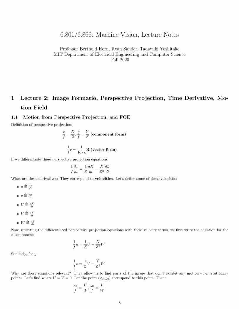
Definition of perspective projection:

x

f=X

Z,y

f=Y

Z(component form)

1

fr =

1

R · zR (vector form)

If we differentiate these perspective projection equations:

1

f

dx

dt=

1

Z

dX

dt− X

Z2

dZ

dt

What are these derivatives? They correspond to velocities. Let’s define some of these velocities:

• u ∆= dx

dt

• v ∆= dy

dt

• U ∆= dX

dt

• V ∆= dY

dt

• W ∆= dZ

dt

Now, rewriting the differentiated perspective projection equations with these velocity terms, we first write the equation for thex component:

1

fu =

1

ZU − X

Z2W

Similarly, for y:

1

fv =

1

ZV − Y

Z2W

Why are these equations relevant? They allow us to find parts of the image that don’t exhibit any motion - i.e. stationarypoints. Let’s find where U = V = 0. Let the point (x0, y0) correspond to this point. Then:

x0

f=

U

W,y0

f=

V

W

8

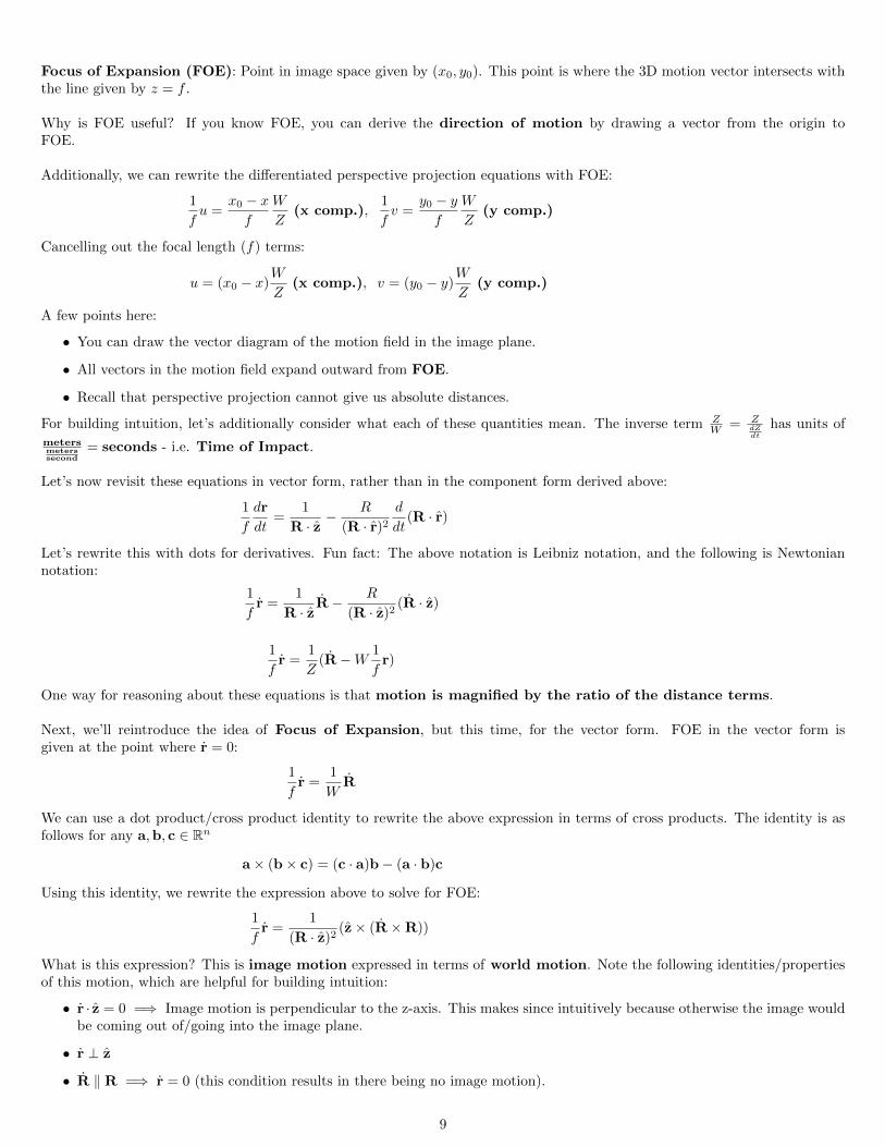
Focus of Expansion (FOE): Point in image space given by (x0, y0). This point is where the 3D motion vector intersects withthe line given by z = f .

Why is FOE useful? If you know FOE, you can derive the direction of motion by drawing a vector from the origin toFOE.

Additionally, we can rewrite the differentiated perspective projection equations with FOE:

1

fu =

x0 − xf

W

Z(x comp.),

1

fv =

y0 − yf

W

Z(y comp.)

Cancelling out the focal length (f) terms:

u = (x0 − x)W

Z(x comp.), v = (y0 − y)

W

Z(y comp.)

A few points here:

• You can draw the vector diagram of the motion field in the image plane.

• All vectors in the motion field expand outward from FOE.

• Recall that perspective projection cannot give us absolute distances.

For building intuition, let’s additionally consider what each of these quantities mean. The inverse term ZW = Z

dZdt

has units ofmetersmeterssecond

= seconds - i.e. Time of Impact.

Let’s now revisit these equations in vector form, rather than in the component form derived above:

1

f

dr

dt=

1

R · z− R

(R · r)2

d

dt(R · r)

Let’s rewrite this with dots for derivatives. Fun fact: The above notation is Leibniz notation, and the following is Newtoniannotation:

1

fr =

1

R · zR− R

(R · z)2(R · z)

1

fr =

1

Z(R−W 1

fr)

One way for reasoning about these equations is that motion is magnified by the ratio of the distance terms.

Next, we’ll reintroduce the idea of Focus of Expansion, but this time, for the vector form. FOE in the vector form isgiven at the point where r = 0:

1

fr =

1

WR

We can use a dot product/cross product identity to rewrite the above expression in terms of cross products. The identity is asfollows for any a,b, c ∈ Rn

a× (b× c) = (c · a)b− (a · b)c

Using this identity, we rewrite the expression above to solve for FOE:

1

fr =

1

(R · z)2(z× (R×R))

What is this expression? This is image motion expressed in terms of world motion. Note the following identities/propertiesof this motion, which are helpful for building intuition:

• r · z = 0 =⇒ Image motion is perpendicular to the z-axis. This makes since intuitively because otherwise the image wouldbe coming out of/going into the image plane.

• r ⊥ z

• R ‖ R =⇒ r = 0 (this condition results in there being no image motion).

9

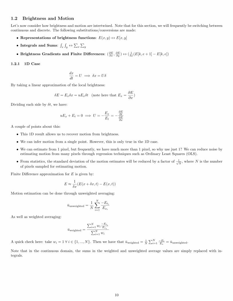
1.2 Brightness and Motion

Let’s now consider how brightness and motion are intertwined. Note that for this section, we will frequently be switching betweencontinuous and discrete. The following substitutions/conversions are made:

• Representations of brightness functions: E(x, y)↔ E[x, y]

• Integrals and Sums:∫x

∫y↔∑x

∑y

• Brightness Gradients and Finite Differences: (∂E∂x ,∂E∂y )↔ ( 1

δx (E[k, e+ 1]− E[k, e])

1.2.1 1D Case

dx

dt= U =⇒ δx = Uδ

By taking a linear approximation of the local brightness:

δE = Exδx = uExδt (note here that Ex =∂E

∂x)

Dividing each side by δt, we have:

uEx + Et = 0 =⇒ U = −ExEt

= −∂E∂t∂E∂x

A couple of points about this:

• This 1D result allows us to recover motion from brightness.

• We can infer motion from a single point. However, this is only true in the 1D case.

• We can estimate from 1 pixel, but frequently, we have much more than 1 pixel, so why use just 1? We can reduce noise byestimating motion from many pixels through regression techniques such as Ordinary Least Squares (OLS).

• From statistics, the standard deviation of the motion estimates will be reduced by a factor of 1√N

, where N is the number

of pixels sampled for estimating motion.

Finite Difference approximation for E is given by:

E ≈ 1

δx(E(x+ δx, t)− E(x, t))

Motion estimation can be done through unweighted averaging:

uunweighted =1

N

N∑i=1

−EtiExi

As well as weighted averaging:

uweighted =

∑Ni=1 wi

−EtiExi∑N

i=1 wi

A quick check here: take wi = 1 ∀ i ∈ 1, ..., N. Then we have that uweighted = 1N

∑Ni=1

−EtEx

= uunweighted.

Note that in the continuous domain, the sums in the weighted and unweighted average values are simply replaced with in-tegrals.

10

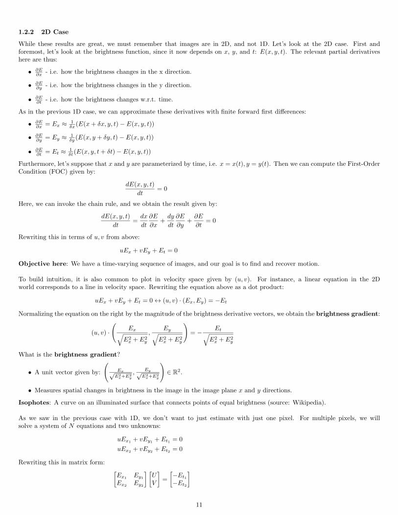
1.2.2 2D Case

While these results are great, we must remember that images are in 2D, and not 1D. Let’s look at the 2D case. First andforemost, let’s look at the brightness function, since it now depends on x, y, and t: E(x, y, t). The relevant partial derivativeshere are thus:

• ∂E∂x - i.e. how the brightness changes in the x direction.

• ∂E∂y - i.e. how the brightness changes in the y direction.

• ∂E∂t - i.e. how the brightness changes w.r.t. time.

As in the previous 1D case, we can approximate these derivatives with finite forward first differences:

• ∂E∂x = Ex ≈ 1

δx (E(x+ δx, y, t)− E(x, y, t))

• ∂E∂y = Ey ≈ 1

δy (E(x, y + δy, t)− E(x, y, t))

• ∂E∂t = Et ≈ 1

δt (E(x, y, t+ δt)− E(x, y, t))

Furthermore, let’s suppose that x and y are parameterized by time, i.e. x = x(t), y = y(t). Then we can compute the First-OrderCondition (FOC) given by:

dE(x, y, t)

dt= 0

Here, we can invoke the chain rule, and we obtain the result given by:

dE(x, y, t)

dt=dx

dt

∂E

∂x+dy

dt

∂E

∂y+∂E

∂t= 0

Rewriting this in terms of u, v from above:

uEx + vEy + Et = 0

Objective here: We have a time-varying sequence of images, and our goal is to find and recover motion.

To build intuition, it is also common to plot in velocity space given by (u, v). For instance, a linear equation in the 2Dworld corresponds to a line in velocity space. Rewriting the equation above as a dot product:

uEx + vEy + Et = 0↔ (u, v) · (Ex, Ey) = −Et

Normalizing the equation on the right by the magnitude of the brightness derivative vectors, we obtain the brightness gradient:

(u, v) ·

(Ex√

E2x + E2

y

,Ey√

E2x + E2

y

)= − Et√

E2x + E2

y

What is the brightness gradient?

• A unit vector given by:

(Ex√E2x+E2

y

,Ey√E2x+E2

y

)∈ R2.

• Measures spatial changes in brightness in the image in the image plane x and y directions.

Isophotes: A curve on an illuminated surface that connects points of equal brightness (source: Wikipedia).

As we saw in the previous case with 1D, we don’t want to just estimate with just one pixel. For multiple pixels, we willsolve a system of N equations and two unknowns:

uEx1+ vEy1 + Et1 = 0

uEx2+ vEy2 + Et2 = 0

Rewriting this in matrix form: [Ex1 Ey1Ex2 Ey2

] [UV

]=

[−Et1−Et2

]

11

Solving this as a standard Ax = b problem, we have:[UV

]=

1

(Ex1Ey2 − Ey1Ex2

)

[Ey2 −Ey1−Ex2

Ex1

] [−Et1−Et2

]Note that the expression given by 1

(Ex1Ey2−Ey1Ex2 ) is the determinant of the partial derivatives matrix, since we are taking its

inverse (in this case, simply a 2x2 matrix).

When can/does this fail? It’s important to be cognizant of edge cases in which this motion estimation procedure/algo-rithm fails. Some cases to consider:

• When brightness partial derivatives / brightness gradients are parallel to one another ↔ The determinant goes to zero ↔This corresponds to linear dependence in the observations. This occurs when Ex1Ey2 = Ey1Ex2 =⇒ Ey1

Ex1=

Ey2Ex2

.

This issue can be mitigated by weighting the pixels as we saw in the 1D case above. However, a more robust solution is to searchfor a minima of motion, rather than the point where it has zero motion. The intuition here is that even if we aren’t able to finda point of zero motion, we can still get as close to zero as possible. Mathematically, let us define the following objective:

J(u, v)∆=

∫x∈X

∫y∈Y

(uEx + vEy + Et)2dxdy

Then we now seek to solve the problem of:

u∗, v∗ = arg minu,v

J(u, v) = arg minu,v

∫x∈X

∫y∈Y

(uEx + vEy + Et)2dxdy

Since this is an unconstrained optimization problem, we can solve by finding the minimum of the two variables using twoFirst-Order Conditions (FOCs):

• ∂J(u,v)∂u = 0

• ∂J(u,v)∂v = 0

Here, we have two equations and two unknowns. When can this fail?

• When we have linear independence. This occurs when:

– E = 0 everywhere

– E = constant

– Ex = 0

– Ey = 0

– Ex = Ey

– Ex = kEy

• When E = 0 everywhere (professor’s intuition: “You’re in a mine.”)

• When Ex, Ey = 0 (constant brightness).

• Mathematically, this fails when:∫x

∫xE2x

∫y

∫yE2y − (

∫x

∫yExEy)2 = 0

When is this approach possible? Only when isophotes are not parallel straight lines - i.e. want isophote curva-ture/rapid turning of brightness gradients.

Noise Gain: Intuition - if I change a value by this much in the image, how much does this change in the result?

2 Lecture 3: Time to Contact, Focus of Expansion, Direct Motion VisionMethods, Noise Gain

2.1 Noise Gain

Example/motivation: Indoor GPS. Rather than using localization of position with satellites, use indoor cellular signals.

Fun fact: EM waves travel at 1 ns/foot.

Dilution of Precision:

12

• How far off GPS is w.r.t. your location.

• Important to note that your dilution of precision can vary in different directions - e.g. horizontal precision is oftentimesgreater than vertical position.

2.2 Forward and Inverse Problems of Machine Vision

2.2.1 Scalar Case

One way to conceptualize the goals of machine vision, as well as to highlight why noise gain is important, is by considering thefollowing problems with some one-dimensional input x and an output y = f(x):

• The forward problem: x→ y∆= f(x)

• The inverse problem∗: y∆= f(x)→ x

*(this term comes up a lot in machine vision, computer graphics, and robotics)

In machine vision, we oftentimes focus on solving the inverse problem, rather than the forward problem. Intuitively, weusually observe some y = f(x), and from this infer the latent parameters x using our model f .

When it is possible to express the inverse of a function in closed form or via a matrix/coefficient, we can simply solve theinverse problem using: x = f−1(y).

More importantly, to build a robust machine vision system to solve this inverse problem, it is critical that small perturbations iny = f(x) do not need to large changes in x. Small perturbations need to be taken into account in machine vision problems be-cause the sensors we use exhibit measurement noise. The concept of noise gain can come in to help deal with this uncertainty.

Consider a perturbation δy that leads to a perturbation δx when we solve the inverse problem. In the limit, as δ ∈ R→ 0, thenwe arrive at the definition of noise gain:

noise gain =δx

δy=

1

f ′(x)=

1df(x)dx

(1)

Like other concepts/techniques we’ve studied so far, let’s understand when this system fails. Below are two cases; we encourageto consider why they fail from both a mathematical and intuitive perspective (hint: for the mathematical component, look atthe formula above, and for the intuitive component, think about how the effect on x from a small change in y in a curve that isnearly flat):

• f ′(x) = 0 (flat curve)

• f ′(x) ≈ 0 (nearly flat curve)

2.2.2 Vector Case

Now that we’ve analyzed this problem in the scalar case, let us now consider it in the vector/multi-dimensional case. Sinceimages are inherently multidimensional, this more general vector case is where we will find ourselves.

First, we can restate these problems:

• Forward Problem: x = Mb,M ∈ Rm×n for m,n ∈ N

• Inverse Problem: b = M−1x,M ∈ Rm×n for m,n ∈ N

But how good is this answer/approach? If x changes, how much does b change? We quantify noise gain in this case as follows:

“noise gain”→ ||δb||||δx||

, δ ∈ R (2)

*NOTE: This multidimensional problem is more nuanced because we may be in the presence of an anisotropic (spatiallynon-uniform) noise gain - e.g. there could be little noise gain in the x1 direction, but a lot of noise gain in the x2 direction.

13

As in the previous case, let’s analyze when this approach fails. To do this, let’s consider M−1 to help build intuition forwhy this fails:

M−1 =1

det|M |

· · ·· · ·· · ·

(3)

Let’s ignore the specific entries of M−1 for now, and focus on the fact that we need to compute the determinant of M . When isthis determinant zero? This will be the case whenever there exists linear dependence in the columns of M. As we saw before,two cases that can yield to poor performance will be:

• det|M | = 0: This corresponds to a non-invertible matrix, and also causes the noise term to blow up.

• det|M | ≈ 0: Though this matrix may be invertible, it may cause numerical instability in the machine vision system, andcan also cause the noise term to blow up.

Let’s also revisit, just as a refresher, the inverse of a 2 × 2 matrix:

A =

[a bc d

](4)

(5)

A−1 =1

detA

[d −b−c a

]=

1

ad− bc

[d −b−c a

](6)

Now let’s verify that this is indeed the inverse:

A−1A =1

ad− bc

[d −b−c a

] [a bc d

]=

1

ad− bc

[ad− bc −ab+ abcd− cd ad− bc

]=

[1 00 1

]= I2 (7)

2.3 Review from Lecture 2

Before we dive into the next set of concepts, let’s also revisit some of the concepts discussed in the previous lectures.

2.3.1 Two-Pixel Motion Estimation, Vector Form

First, let’s recall the two pixel motion estimation set of equations:

uEx1+ vEy1 + Et1 = 0 (8)

uEx2+ vEy2 + Et2 = 0 (9)

Rewritten in matrix form: [uv

]=

1

Ex1Ey2 − Ey1Ex2

[Ey2 −Ey1−Ex2

Ex1

](10)

Take note of the denominator on the right-hand side. Does this term look familiar to the determinant term above? We wereindeed solving an instance of the inverse problem. If this determinant-like quantity (Ex1Ey2 − Ey1Ex2) is small, the noise isgreatly amplified. We saw that this happens when brightness gradients are similar to one another.

2.3.2 Constant Brightness Assumption, and Motion Equation Derivation

Recall the constant brightness assumption’s mathematical formulation:

Constant Brightness Assumption =⇒ dE

dt= 0 (11)

*(Please note the quantity above is a total derivative.)

Intuition Behind This: As the object/camera moves, the physical properties of the camera do not change and thereforethe total derivative of the brightness w.r.t. time is 0. From the chain rule, we can rewrite this total derivative assumption:

dE

dt= 0 =⇒ uEx + vEy + Et = 0 (12)

*(Recall this is for when x and y are parameterized w.r.t. time, i.e. x = x(t), y = y(t).)

The above constraint is known as the Brightness Change Constraint Equation (BCCE).

14

2.3.3 Optical Mouse Problem

Recall our motion estimation problem with the optical mouse, in which our objective is no longer to find the point where theBCCE is strictly zero (since images are frequently corrupted by noise through sensing), but to minimize the LHS of the BCCE,i.e:

minu,vJ(u, v)

∆=

∫∫(uEx + vEy + Et)

2dxdy (13)

We solve the above using unconstrained optimization and by taking a “least-squares” approach (hence why we square the LHSof the BCCE). Solve by setting the derivatives of the two optimizing variables to zero:

dJ(u, v)

du= 0,

dJ(u, v)

dv= 0 (14)

2.3.4 Perspective Projection

Recall the perspective projection equations in the scalar form:

x

f=X

Z(x-component),

y

f=Y

Z(y-component) (15)

*(Note that capital coordinates are in the world space, and lowercase coordinates are in the image space.)

What if these quantities are changing in the world w.r.t. time? Take time derivatives:

1

f

dx

dt=

1

Z

dX

dt− 1

Z2XdZ

dt(16)

Writing these for x and y:

• x: 1f u = 1

ZU −WZXZ

• y: 1f v = 1

ZV −WZYZ

Note again the following definitions:

• u→ image velocity in the x direction

• v → image velocity in the y direction

• U → world velocity in the X direction

• V → world velocity in the Y direction

When are these points in (u, v) space interesting? When u = v = 0 - this is the Focus of Expansion (FOE). The FOE givenby (x0, y0) in two dimensions:

(x0, y0) = (f

Z

U

W,f

Z

V

W) (17)

2.4 Time to Contact (TTC)

In the previous lecture, we discussed the derivation of Time to Contact (TTC) in terms of meters:

Z

W

∆==

ZdZdt

=metersmetersseconds

= seconds (18)

Let us express the inverse of this Time to Contact (TTC) quantity as C:

C∆=W

Z=

1

TTC(19)

Let us now suppose we parameterize our spatial velocities u and v according to u = Cx, v = Cy, where C is the inverse TTCvalue we introduced above. Then, substituting these into the BCCE equation, we have:

Recall BCCE: uEx + vEy + Et = 0 (20)

Substitute: C(xEx + yEy) + Et = 0 (21)

Solve for C: C = − EtxEx + yEy

(22)

15

The denominator in the derivation of C is the “radial gradient”:

g = xEx + yEy = (x, y) · (Ex, Ey) (23)

Building Intuition: If we conceptualize 2D images as topographic maps, where brightness is the third dimension of the surface(and the spatial dimensions x and y comprise the other two dimensions), then the brightness gradient is the direction of steepestascent up the brightness surface.

Another note: (x, y) is a radial vector, say in a polar coordinate system. Hence why the above dot product term is coinedthe name “radial gradient”. This gradient is typically normalized by its L2/Euclidean norm to illustrate the multiplication ofthe brightness gradients with a radial unit vector):

g =√x2 + y2(

x√x2 + y2

,y√

x2 + y2) · (Ex, Ey) (24)

This g quantity can be thought of as: “How much brightness variation is in an outward direction from the center of the image?”

For a more robust estimate, let us again employ the philosophy that estimating from more data points is better. We’ll againtake a least-squares approach, and minimize across the entire image using the parameterized velocities we had before. In thiscase, since we are solving for inverse Time to Contact, we will minimize the error term over this quantity:

minCJ(C)

∆=

∫∫(C(xEx + yEy) + Et)

2dxdy (25)

Without the presence of measurement noise, the optimal value of C gives us an error of zero, i.e. perfect adherence to theBCCE. However, as we’ve seen with other cases, this is not the case in practice due to noise corruption. We again will useunconstrained optimization to solve this problem.

Taking the derivative of the objective J(C) and setting it to zero, we obtain:

dJ(C)

dC= 0 =⇒ 2

∫∫(C(xEx + yEy) + Et)(xEx + yEy)dxdy = 0 (26)

This in turn gives us:

C

∫∫(xEx + yEy)2dxdy +

∫∫(xEx + yEy)Etdxdy = 0 (27)

1

TTC= C = −

∫∫(xEx + yEy)Etdxdy∫∫(xEx + yEy)2dxdy

(28)

A few notes here:

• Et can be computed by taking differences between a pixel at different points in time.

• To implement a framework like this, we can do so with accumulators.

• This is an instance of “direct computation”.

• When objects/important components of a scene are far away, we can combine image pixels and run these algorithms atmultiple scales - this allows us to compute/analyze motion velocities over different timescales. This can also be helpfulfor building more computationally-tractable motion estimation implementations, since the number of pixels over whichcomputations must occur can be reduced quadratically with the scale.

• Note one problem we run into with this approach - each pixel we apply this estimation approach to introduces one equation,but two unknowns.

• Note that neighboring pixels typically exhibit similar behavior to one another.

Let’s briefly return to the concept of the radial gradient. When is this zero?

• E = 0 everywhere (coal mine)

• (x, y) · (Ex, Ey) = 0 (radial gradient is zero)

Now, let’s take a more general case when we have world motion, i.e. U 6= 0, V 6= 0. For our two components x and y:

16

• x-component:

u

f=U

Z− X

f

W

Z(29)

u =fU

Z−XW

Z(30)

u = A−XC (31)

Where: A∆=fU

Z,C

∆=W

Z(32)

• y-component:

v

f=V

Z− Y

f

W

Z(33)

v =fV

Z− Y W

Z(34)

v = B − Y C (35)

Where: B∆=fV

Z,C

∆=W

Z(36)

Note that for the world quantities A and B, we also have the following identities (note that the Focus of Expansion (FOE) isgiven by the point (x0, y0):

• A = fUZ = Cx0

• B = fVZ = Cy0

Building Intuition: “As I approach the wall, it will loom outward and increase in size.”

Now returning to our BCCE, this time with A, B, and C:

AEx +BEy + C(xEx + yEy) + Et = 0 (37)

We can again use least-squares to minimize the following objective enforcing the BCCE. This time, our optimization aim is tominimize the objective function J(A,B,C) using the quantities A, B, and C:

minA,B,C

J(A,B,C) ∆=

∫∫(AEx +BEy + C(xEx + yEy) + Et)

2dxdy (38)

Use unconstrained optimzation with calculus and partial derivatives to solve. Since we have three variables to optimize over, wehave three first-order conditions (FOCs):

• dJ(A,B,C)dA = 0

• dJ(A,B,C)dB = 0

• dJ(A,B,C)dC = 0

Using the Chain rule for each of these FOCs, we can derive and rewrite each of these conditions to obtain 3 equations and 3

unknowns. Note that G∆= xEx + yEy.

• A variable:

2

∫∫(AEx +BEy + C(xEx + yEy))Ex = 0 (39)

A

∫∫E2x +B

∫∫ExEy + C

∫∫GEx = −

∫∫ExEt (40)

• B variable:

2

∫∫(AEx +BEy + C(xEx + yEy))Ex = 0 (41)

A

∫∫EyEx +B

∫∫E2y + C

∫∫GEy = −

∫∫EyEt (42)

17

• C variable:

2

∫∫(AEx +BEy + C(xEx + yEy))Ex = 0 (43)

A

∫∫GEx +B

∫∫GEy + C

∫∫G2 = −

∫∫GEt (44)

Putting all of these equations together:

A

∫∫E2x +B

∫∫ExEy + C

∫∫GEx = −

∫∫ExEt

A

∫∫EyEx +B

∫∫E2y + C

∫∫GEy = −

∫∫EyEt

A

∫∫GEx +B

∫∫GEy + C

∫∫G2 = −

∫∫GEt

This can be compactly written as a matrix-vector product equation:∫∫

E2x

∫∫ExEy

∫∫ExG∫∫

EyEx∫∫

E2y

∫∫EyG∫∫

GEx∫∫

GEy∫∫

G2

ABC

= −

∫∫ ExEt∫∫EyEt∫∫GEt

As in the time-to-contact problem above, this can again be implemented using accumulators.

Let’s end on a fun fact: Did you know that optical mice have frame rates of 1800 fps?

3 Lecture 4: Fixed Optical Flow, Optical Mouse, Constant Brightness As-sumption, Closed Form Solution

3.1 Review

Let’s frame the topics today by briefly reviewing some concepts we’ve covered in the previous lectures. Feel free to skip thissection if you already feel comfortable with the material.

• Image formation

– Where in the image? Recall perspective projection:

x

f=X

Z,y

f=Y

Z

Differentiating this expression gives:

u

f=U

Z− X

Z

W

Z,v

f=V

Z− Y

Z

W

Z

From these, we can find the Focus of Expansion (FOE), or, more intuitively: “The point in the image towardwhich you are moving.”

How long until we reach this point? This is given by Time to Contact (TTC):

Time to Contact =Z

W=

1

C

– How bright in the image? For this, let us consider an image solid, where the brightness function is parameterized byx, y, and t: E(x, y, t).

18

3.1.1 Constant Brightness Assumption Review with Generalized Isophotes

Recall the constant brightness assumption, which says that the total derivative of brightness with respect to time is zero:dE(x,y,t)

dt = 0. By chain rule we obtain the BCCE:

dx

dt

∂E

∂x+dy

dt

∂E

∂y+∂E

∂t= 0

Recall our variables: u∆= dx

dt , v∆= dy

dt . Then BCCE rewritten in the standard notation we’ve been using:

uEx + yEy + Et = 0

Recall our method of using least-squares regression to solve for optimal values of u, v that minimize the total computed sumof the LHS of the BCCE over the entire image (note that integrals become discrete in the presence of discretized pixels, andderivatives become differences):

u∗, v∗ = arg minu,v

∫∫(uEx + yEy + Et)dxdy

The first-order conditions (FOCs) of this optimization problem give:

u

∫∫E2x + v

∫∫ExEy = −

∫∫ExEt (45)

u

∫∫EyEx + v

∫∫E2y = −

∫∫EyEt (46)

Written in matrix-vector form, our equations become:[ ∫∫E2x

∫∫ExEy∫∫

EyEx∫∫

E2y

] [uv

]= −

[∫∫ExEt∫∫EyEt

](New) Now, to introduce a new variation on this problem, let us suppose we have the following spatial parameterization ofbrightness (you’ll see that this brightness function creates linear isophotes) for linear f :

E(x, y) = f(ax+ by)

If f is differentiable over the domain, then the spatial derivatives Ex and Ey can be computed as follows, using the chain rule:

• Ex = f ′(ax+ by)a

• Ey = f ′(ax+ by)b

Where f ′ is the derivative of this scalar-valued function (i.e, we can define the input to be z = ax+ by, and the derivative f ′ is

therefore equivalent to df(z)dz ).

Isophote Example: If E(x, y) = ax + by + c, for a, b, c ∈ R+, then the isophotes of this brightness function will be lin-ear.

3.1.2 Time to Contact (TTC) Review

Recall the following symbols/quantities from TTC:

• C = Zw

• TTC = wZ = 1

ZdZdt = d

dt loge(z) , therefore we can simply take the slope of the line corresponding to the logarithm of Z tocompute TTC.

Now, let’s suppose that objects are moving both in the world and in the image. Let’s denote s as our image coordinate and Sas our world coordinate. Then:

s

f=S

Z

Then we can write:

sZ + sf = 0

19

Differentiating:

Zds

dt+ s

dZ

dt= 0 =⇒

dsdt

S=

dZdt

Z

The above relationship between derivative ratios can be interpreted as: “The change in the image’s size is the same as the changein distance.”

3.2 Increasing Generality of TTC Problems

Let us now consider adding some additional generality to the Time to Contact (TTC) problem. We’ve already visited some ofthese cases before:

• Simple case: Solving for C

• More General case: Solving for A,B,C

• Even More General case: (Motivation) What if the optical axis isn’t perpendicular to the wall? What if the cameraplane is tilted, e.g. Z = aX + bY + C for some a, b, C ∈ R? In this case, we can solve the problem numerically ratherthan through a closed-form expression.

Another motivating question for developing TTC methods: What if the surface is non-planar? This is a common scenario forreal-world TTC systems. In this case, we have two options:

• Parameterize the geometric models of these equations with polynomials, rather than planes.

• Leave the planar solution, and look for other ways to account for errors between the modeled and true surfaces.

In practice, the second option here actually works better. The first option allows for higher modelling precision, but is less robustto local optima, and can increase the sensitivity of the parameters we find through least-squares optimization.

If you want to draw an analog to machine learning/statistics, we can think of modeling surfaces with more parameters (e.g.polynomials rather than planes) as creating a model that will overfit or not generalize well to the data it learns on, and createa problem with too many unknowns and not enough equations.

3.3 Multiscale and TTC

If you recall from last lecture, we saw that TTC and FOE estimation “fell apart” as we got really close. This is due to mea-surement sensitivity and the fact that the pixels occupy increasingly more space as we get closer and closer. This is wheremultiscale can help us - it enables us to use more coarse resolutions for these estimation problems. The implicit averaging donethrough downsampling allows us to “smoooth out” any measurement noise that may be present, and will consequently reducethe magnitide of pixel brightness gradients.

Additionally, multiscale is computationally-efficient: Using the infinite geometric series, we can see that downsampling/down-scaling by a factor of 2 each time and storing all of these smaller image representations requires only 33% more stored data thanthe full size image itself:

∞∑n=0

((1

2)2)n =

1

1− 14

=4

3= 1 +

1

3

More generally, for any downsampling factor r ∈ N, we only add 1r2−1 × 100% amount of additional data:

∞∑n=0

(1

r2)n =

1

1− 1r2

=r2

r2 − 1=

(r2 − 1) + 1

r2 − 1= 1 +

1

r2 − 1

(Note that we have r2 rather than r in the denominator because we are downsampling across both the x and y dimensions.)

20

3.3.1 Aliasing and Nyquist’s Sampling Theorem

Though multiscale is great, we also have to be mindful of aliasing. Recall from 6.003 (or another Signals and Systems course)that aliasing causes overlap and distortion between signals in the frequency domain, and it is required that we sample at a spatialfrequency that is high enough to not produce aliasing artifacts.

Nyquist’s Sampling Theorem states that we must sample at twice the frequency of the highest-varying component of our imageto avoid aliasing and consequently reducing spatial artifacts.

3.3.2 Applications of TTC

A few more applications of TTC:

• Airplane Wing Safety - Using TTC to make sure wings don’t crash into any objects at airports.

• NASA TTC Control - TTC systems were used to ensure that NASA’s payload doesn’t crash into the surface of earth/otherplanets/moons. In this application, feedback control was achieved by setting a nominal “desired TTC” and using anamplifier, imaging, and TTC estimation to maintain this desired TTC.

• Autonomous Vehicles - e.g. a vehicle is coming out of a parking lot and approaching a bus - how do we control when/if tobrake?

Let’s discuss the NASA TTC Control example a little further. Using our equation for TTC:

Z

W= T

We can rewrite this as a first-order Ordinary Differential Equation (ODE):

ZdZdt

= T =⇒ dZ

dt=

1

TZ

Since the derivative of Z is proportional to Z, the solution to this ODE will be an exponential function in time:

Z(t) = Z0e−tT

Where Z0 depends on the initial conditions of the system.

This method requires that deceleration is not uniform, which is not the most energy efficient approach for solving this problem.As you can imagine, energy conservation is very important in space missions, so let’s next consider a constant deceleration

approach. Note that under constant deceleration, we have d2zdt2

∆= a = 0. Then we can express the first derivative of Z w.r.t. t as:

dZ

dt= at+ v0

Where v0 is an initial velocity determined by the boundary/initial conditions. Here we have the following boundary condition:

dZ

dt= a(t− t0)

This boundary condition gives rise to the following solution:

Z =1

2at2 − at0t+ c =

1

2a(t− t0)2

Therefore, the TTC for this example becomes:

T =ZdZdt

=12a(t− t0)2

a(t− t0)=

1

2(t− t0)

21

3.4 Optical Flow

Motivating question: What if the motion of an image is non-constant, or it doesn’t move together? We have the BrightnessChange Constraint Equation (BCCE), but this only introduces one constraint to solve for two variables, and thus createsan under-constrained/ill-posed problem.

How can we impose additional constraints? To do this, let us first understand how motion relates across pixels, andinformation that they share. Pixels don’t necessarily move exactly together, but they move together in similar patterns, partic-ularly if pixels are close to one another. We’ll revisit this point in later lectures.

What Else Can We Do? One solution is to divide the images into equal-sized patches and apply the Fixed Flow Paradigm,as we’ve done with entire images before. When selecting patch size, one trade-off to be mindful of is that the smaller the patch,the more uniform the brightness patterns will be across the patch, and patches may be too uniform to detect motion (note: thisis equivalent to the matrix determinants we’ve been looking at evaluating to zero/near-zero).

3.5 Vanishing Points (Perspective Projection)

Before we dive into what vanishing points are, let’s discuss why they’re useful. Vanishing points can be useful for:

• Camera calibration - has applications to robotics, autonomous vehicles, photogrammetry, etc.

• Finding relative orientation between two coordinate frames/systems

Now, let’s discuss what it is. Suppose we have several parallel lines in the world, and we image them by projecting them ontothe 2D image plane. Then vanishing points are the points in the image (or, more commonly, outside of the image) where theselines converge to in the image. To discuss these mathematically, let’s first discuss about defining lines in a 3D world:

• Vector Form: R = R0 + snHere, we can express this using our standard vector form of perspective projection:

1

fr =

1

R · zR

=1

(R0 + sn) · n(R0 + sn)

• Parametrically: (x0 + αs, y0 + βs, z0 + γs)Here, we can expand this to our standard Cartesian form of perspective projection to apply our transformation:

x

f=

1

Z0 + γs(x0 + αs)

y

f=

1

Z0 + γs(y0 + βs)

To build intuition, let’s consider what happens when we travel far along the lines (i.e. as s gets very large) in our parametricdefinition of lines:

• limx→∞xf = limx→∞

1Z0+γs (x0 + αs) = αs

γs = αγ (x-coordinate)

• limy→∞yf = limy→∞

1Z0+γs (x0 + βs) = βs

γs = βγ (x-coordinate)

The 2D point (αγ ,βγ ) is the vanishing point in the image plane. As we move along the line in the world, we approach this point

in the image, but we will never reach it. More generally, we claim that parallel lines in the world have the same vanishingpoint in the image.

3.5.1 Applications of Vanishing Points

Let’s now discuss some of these applications in greater detail.

• Protecting Pedestrians on a Road Side: To protect pedestrians, the camera must transform its coordinate system.This transformation can be found using vanishing points.

• Camera Calibration: One way to calibrate a camera is to solve for the Center of Projection (COP) in the imagespace, using perspective projection. Calibration is typically achieved through calibration objects.

22

3.6 Calibration Objects

Let’s discuss two calibration objects: spheres and cubes:

3.6.1 Spheres

:

• If image projection is directly overhead/straight-on, the projection from the world sphere to the image plane is a circle. Ifit is not overhead/straight on, it is elliptic.

• Relatively easy to manufacture

3.6.2 Cube

:

• Harder to manufacture, but generally a better calibration object than a sphere.

• Cubes can be used for detecting edges, which in turn can be used to find vanishing points (since edges are lines in theworld).

• Cubes have three sets of four parallel lines/edges each, and each of these sets of lines are orthogonal to the others. Thisimplies that we will have three vanishing points - one for each set of parallel lines.

• For each of these sets of lines, we can pick a line that goes through the Center of Projection (COP), denoted p ∈ R3 (inthe world plane). We can then project the COP onto the image plane (and therefore now p ∈ R2).

• Let us denote the vanishing points of the cube in the image plane as a,b, c ∈ R2. Then, because of orthogonality betweenthe different sets of lines, we have the following relations between our three vanishing points and p:

– (p− a) · (p− b) = 0

– (p− b) · (p− c) = 0

– (p− c) · (p− a) = 0

In other words, the difference vectors between p and the vanishing points are all at right angles to each other.

To find p, we have three equations and three unknowns. We have terms that are quadratic in p. Using Bezout’sTheorem (The maximum number of solutions is the product of the polynomial order of each equation in the system ofequations), we have (2)3 = 8 possible solutions for our system of equations. More generally:

number of solutions =E∏e=1

oe

Whhere E is the number of equations and oe is the polynomial order of the eth equation in the system.

This is too many equations to work with, but we can subtract these equations from one another and create a systemof 3 linearly dependent equations. Or, even better, we can leave one equation in its quadratic form, and 2 in their linearform, and this maintains linear independence of this system of equations:

– (a− p) · (c− b) = 0

– (b− p) · (a− c) = 0

– (p− c) · (p− a) = 0

3.7 Additional Topics

We’ll also briefly recap some of the topics discussed in our synchronous section today. These topics are not meant to introducenew concepts, but are designed to generalize the concepts we’ve discussed such that they can be adapted for a broader range ofapplications.

23

3.7.1 Generalization: Fixed Flow

The motivating example for this generalization is a rotating optimal mouse. We’ll see that instead of just solving for our twovelocity parameters u and v, we’ll also need to solve for our rotational velocity, ω.

Suppose we are given the following parameterizations of velocity:

• u = u0 − wy

• v = v0 + wx

Note that we can also write the radial vector of x and y, as well as the angle in this 2D plane to show how this connects torotation:

r = (x, y) =√x2 + y2

θ = arctan 2(y, x)

ω =dθ

dt

With this rotation variable, we leverage the same least-squares approach as before over the entirety of the image, but now wealso optimize over the variable for ω:

u∗0, v∗0 , ω

∗ = arg minu0,v0,ω

J(u0, v0, ω)∆=

∫∫(u0Ex + v0Ey + wH + Et)

2dxdy

Like the other least-squares optimization problems we’ve encountered before, this problem can be solved by solving a system offirst-order conditions (FOCs):

• dJ(u0,v0,ω)du0

= 0

• dJ(u0,v0,ω)dv0

= 0

• dJ(u0,v0,ω)dω = 0

3.7.2 Generalization: Time to Contact (for U = 0, V = 0, ω 6= 0)

Let’s now revisit TTC, but with the following parameterization: U 6= 0, V 6= 0, image is of a tilted plane.

For this, we can write Z as a function of the world coordinates X and Y :

Z = Z0 +∂Z

∂XX +

∂Z

∂YY

Z = Z0 + pX + qY

Recall the following derivations for the image coordinate velocities u and v, which help us relate image motion in 2D to worldmotion in 3D:

• uf = U

Z −XZWZ

• vf = V

Z −YZWZ

Some additional terms that are helpful when discussing these topics:

• Motion Field: Projection of 3D motion onto the 2D image plane.

• Optical Flow:

– What we can sense

– Describes motion in the image

We can transform this into image coordinates:

u =1

2(fU − xw), v =

1

2(fV − yw)

24

Let’s take U = V = 0, u = −X wZ , v = −Y W

Z . Z (world coordinates) is not constant, so we can rewrite this quantity bysubstituting the image coordinates in for our expression for Z:

Z = Z0 + px+ qy

= Z0 + pX

fZ + q

Y

fZ

Now, we can isolate Z and solve for its closed form:

Z(1− pXf− q Y

f) = Z0

Z =Z0

1− pXf − qYf

From this we can conclude that 1Z is linear in x and y (the image coordinates, not the world coordinates). This is helpful for

methods that operate on finding solutions to linear systems. If we now apply this to the BCCE given by uEx + vEy +Et = 0,we can first express each of the velocities in terms of this derived expression for Z:

• u = 1Z0

(1− pXf − qYf )(−xω)

• v = 1Z0

(1− pXf − qYf )(−yω)

Applying these definitions to the BCCE:

0 = uEx + vEy + Et

=1

Z0(1− pX

f− q Y

f)(−xω)Ex +

1

Z0(1− pX

f− q Y

f)(−yω)Ey + Et

Combining like terms, we can rewrite this constraint as:

0 = − ω

Z0(1− pX

f− q Y

f)(xEx + yEy) + Et

Equivalently, dividing everything by −1:

0 =ω

Z0(1− pX

f− q Y

f)(xEx + yEy)− Et

We can also express this with the “radial gradient” given by: G∆= (xEx + yEy):

0 =ω

Z0(1− pX

f− q Y

f)G− Et

For symbolic simplicity, take the following definitions:

• R ∆= w

Z0

• P ∆= −p wZ0

• Q ∆= −q wZ0

Using these definitions, the BCCE with this paramterization becomes:

0 = (R+ Px+Qy)G− Et

Now, we can again take our standard approach of solving these kinds of problems by applying least-squares to estimate the freevariables P,Q,R over the entire continuous or discrete image space. Like other cases, this fails when the determinant of thesystem involving these equations is zero.

4 Lecture 5: TTC and FOR Montivision Demos, Vanishing Point, Use of VPsin Camera Calibration

In this lecture, we’ll continue going over vanishing points in machine vision, as well as introduce how we can use brightnessestimates to obtain estimates of a surface’s orientation. We’ll introduce this idea with Lambertian surfaces, but we can discusshow this can generalize to many other types of surfaces as well.

25

4.1 Robust Estimation and Sampling

We’ll start by covering some of the topics discussed during lecture.

4.1.1 Line Intersection Least-Squares

Helpful when considering multiple lines at a time - this optimization problem is given by:

minx,y

∑i

(x cos θi + y sin θi − ρ)2 (47)

4.1.2 Dealing with Outliers

Many of the approaches we’ve covered thus far are centered around the idea of making estimates from data. But recall thatthe data gathered by sensors can be noisy, and can be corrupted from phenomena such as crosstalk. Because of this noise,it is advantageous to distinguish and filter outliers from the inliers in our dataset, especially when we make estimates usingLeast-Squares.

A good choice of algorithm for dealing with outliers is RANSAC, or Random Sample Consensus [1]. This algorithmis essentially an iterative and stochastic variation of Least-Squares. By randomly selecting points from an existing dataset to fitlines and evaluate the fit, we can iteratively find line fits that minimize the least-squares error while distinguishing inliers fromoutliers.

Figure 1: Pseudocode for the RANSAC Algorithm.

4.1.3 Reprojection and Rectification

These two problems are highly important in mapmaking, and help for solving the equations:

Rr = r′

r = RT r

Where r is the vector from the Center of Projection (COP) to the image plane.

4.1.4 Resampling

Resampling is also a valuable application in many facets of computer vision and robotics, especially if we seek to run any kindof interpolation or subsampling algorithms. Some approaches for this:

• Nearest Neighbor: This is a class of methods in which we interpolate based off of the values of neighboring points. Thiscan be done spatially (e.g. by looking at adjacent pixels) as well as other image properties such as brightness and color. Acommon algorithm used here is K-Nearest Neighbors (KNN), in which interpolation is done based off of the K-nearestpoints in the desired space.

• Bilinear Interpolation: An extension of linear interpolation used for functions in two-dimensional grids/of two variables(e.g. (x, y) or (i, j))) [2], such as the brightness or motion in images.

26

• Bicubic Interpolation: Similar to bilinear interpolation, bicubic interpolation is an extension of cubic interpolationof functions in two-dimensional grids/of two variables (e.g. (x, y) or (i, j))) [3], such as the brightness or motion inimages. Bicubic interpolation tends to perform much better than bilinear interpolation, though at the cost of additionalcomputational resources.

4.2 Magnification with TTC

• For the Montivision demo, note the following for the bars:

– A→ x-dimension for motion estimation problem

– B → y-dimension for motion estimation problem

– C → 1Time to Contact

• Recall from the previous lectures that the percent change of size in the world is the percent change of size in the image.We can derive this through perspective projection. The equation for this is:

s

f=S

Z

Where s is the size in the image plane and S is the size in the world. Differentiating with respect to time gives us (usingthe chain rule):

d

dt(sZ = fS)→ Z

ds

dt+ s

dZ

dt= 0

Rearranging terms:

dzdt

Zf = −

dsdt

S

Recall that the intuition here is that the rate of change of size is the same in the image and the world.

4.2.1 Perspective Projection and Vanishing Points

Let’s begin by defining a few terms. Some of these will be a review, but these review terms connect to new terms that we’llintroduce shortly:

• vanishing points: These are the points in the image plane (or extended out from the image plane) that parallel lines inthe world converge to.

• Center of Projection (COP): This is where in the camera/sensor (not in the image plane) where incident projectedlight rays converge. An analog to the COP for human vision systems is your eyes. NOTE: COP and vanishing points areoftentimes different.

• Principle Point: The orthogonal projection of the Center of Projection (COP) onto the image plane.

• f : Similar to the focal length we’ve seen in other perspective projection examples, this f is the perpendicular distance fromthe COP to the image plane.

Recall that a common problem we can solve with the use of vanishing points is finding the Center of Projection (COP).Solving this problem in 3D has 3 degrees of freedom, so consequently we’ll try to solve it using three equations.

Intuitively, this problem of finding the Center of Projection can be thought of as finding the intersection of three spheres,each of which have two vanishing points along their diameters. Note that three spheres can intersect in up to two places - in thiscase we have defined the physically-feasible solution, and therefore the solution of interest, to be the solution above the imageplane (the other solution will be a mirror image of this solution and can be found below the image plane).

Application of this problem: This problem comes up frequently in photogrammetry, in that simply having two locations asyour vanishing points isn’t enough to uniquely identify your location on a sphere.

27

4.2.2 Lines in 2D and 3D

Next, let’s briefly review how we can parameterize lines in 2D and 3D:

• 2D: (2 Degrees of Freedom)

– y = mx+ c

– ax+ by + c = 0

– sin θx− cos θy + ρ = 0

– If n∆= (− sin θ, cos θ)T , then n · r = ρ.

• 3D: (3 Degrees of Freedom)

– n = ρ

– aX + bY + cZ + d = 0

4.2.3 Application: Multilateration (MLAT)

This problem comes up when we estimate either our position or the position of other objects based off of Time of Arrival[4]. One specific application of this problem is localizing ourselves using distances/Time of Arrival of wifi access points insidebuildings/other locations without access to GPS.

Like the other problems we’ve looked at, this problem can be solved by finding the intersection of 3 spheres. Let’s beginwith:

||r− ri||2 = pi ∀ i ∈ 1, · · · , N

Next, let’s square both sides of this equation and rewrite the left-hand side with dot products:

||r− ri||22 = (r− ri)T (r− ri) = p2

i

= r · r− 2r · ri + ri · ri = p2i

Recall from Bezout’s Theorem that this means that are 8 possible solutions here, since we have three equations of second-orderpolynomials. To get rid of the 2nd order terms, we simply subtract the equations:

r · r− 2r · ri + ri · ri = ρ2i

− r · r− 2r · rj + rj · rj = ρ2j ∀ i, j ∈ 1, 2, 3, i 6= j

Subtracting these pairs of equations yields a linear equation in R:

2r(rj − ri) = (ρ2j − ρ2

i )− (R2j −R2

i )

(Where the scalar R2j

∆= rj · rj .)

Putting these equations together, this is equivalent to finding the intersection of three different spheres:(r2 − r1)T

r3 − r2)T

r1 − r3)T

r =1

2

(ρ22 − ρ2

1)− (R22 −R2

1)(ρ2

3 − ρ22)− (R2

3 −R22)

(ρ21 − ρ2

3)− (R21 −R2

3)

However, even though we’ve eliminated the second-order terms from these three equations, we still have two solutions. Recallfrom linear algebra equations don’t have a unique solution when there is redundancy or linear dependence between the equations.If we add up the rows on the right-hand side of the previous equation, we get 0, which indicates that the matrix on the left-handside is singular:

A∆=

(r2 − r1)T

r3 − r2)T

r1 − r3)T

∈ R3×3

28

To solve this linear dependence problem, we again use Bezout’s Theorem and keep one of the second-order equations:

(r− r1) · (r− r2) = 0

(r− r2) · (r− r3) = 0

(r− r2) · (r− r2) = 0→ (r− r2) ⊥ (r3 − r1)

I.e. the plane passes through r2 - this intersecting point is the solution and is known as the orthocenter or the principalpoint. Now, all we need is to find the quantity f to find the Center of Projection.

Next, note the following relations between the vanishing points in the inverse plane and z, which lies perpendicular to theimage plane:

r1 · z = 0

r2 · z = 0

r3 · z = 0

What else is this useful for? Here are some other applications:

• Camera calibration (this was the example above)

• Detecting image cropping - e.g. if you have been cropped out of an image

• Photogrammetry - e.g. by verifying if the explorer who claimed he was the first to make it “all the way” to the North Poleactually did (fun fact: he didn’t).

Next, now that we’ve determined the principal point, what can we say about f (the “focal length”)?

For this, let us consider the 3D simplex, which is triangular surface in R3 given by the unit vectors:

e1∆=[1 0 0

]Te2

∆=[0 1 0

]Te3

∆=[0 0 1

]TUsing this 3D simplex, let us suppose that each side of the triangles formed by this simplex take length v =

√2, which is

consistent with the l2 norm of the triangles spanned by the unit simplex (√

12 + 12 =√

2).

Next, we solve for f by finding the value of a such that the dot product between the unit vector perpendicular to the sim-plex and a vector of all a is equal to 1: [

a a a]T [ 1√

31√3

1√3

]T= 1

3a√3

= 1

a =

√3

3=

1√3

This value of a = 1√3

= f . Then we can relate the lengths of the sides v (which correspond to the magnitudes of the vectors

between the principal point and the vanishing points (||r− ri||2)) and f :

v =√

2, f =1√3

=⇒ f =v√6

With this, we’ve now computed both the principal point and the “focal length” f for camera calibration.

4.2.4 Application: Understand Orientation of Camera w.r.t. World

For this problem, the goal is to transform from the world frame of reference to the camera frame of reference, i.e. find a frameof reference such that the unit vectors xc, yc, zc have the following orthogonality properties:

xc · yc ≈ 0

yc · zc ≈ 0

xc · zc ≈ 0

29

(Note that the c superscript refers to the camera coordinate system.) If the location of the Center of Projection (COP) is givenabove the image plane as the vector pc and the vanishing points are given as vectors rc1, rc2, and rc3 (note that these vanishingpoints must be in the same frame of reference in order for this computation to carry out), then we can derive expressions for theunit vectors through the following relations:

(pc − r1)//xc =⇒ xc =pc − rc1||pc − rc1||2

(pc − r2)//yc =⇒ yc =pc − rc2||pc − rc2||2

(pc − r3)//zc =⇒ zc =pc − rc3||pc − rc3||2

Then, after deriving the relative transformation between the world frame (typically denoted w in robotics) and the camera frame(typically denoted c in robotics), we can express the principal point/Center of Projection in the camera coordinate frame:

r = αxc + βyc + γzc

Where (α, β, γ) are the coordinates in the object coordinate system (since xc, yc, and zc comprise the orthogonal basis of thiscoordinate system). Then we can express the relative coordinates of objects in this coordinate system:

r′ =[α β γ

]TTo transform between frames, we can do so via the following equation:

r =

−(xc)T

−(yc)T

−(zc)T

r′

Note that the matrix defined by: R∆=

−(xc)T

−(yc)T

−(zc)T

is orthonormal, since these vector entries are orthogonal to one another.

This matrix R is a rotation matrix, which means it is skew-symmetric, invertible, and its transpose is equal to its inverse:R−1 = RT . Therefore, if we wanted to solve the reverse problem that we did above (finding object coordinates from cameracoordinates), we can do so by simply taking the transpose of the matrix:

r′ =

−(xc)T

−(yc)T

−(zc)T

−1

r

=

−(xc)T

−(yc)T

−(zc)T

T

r

4.3 Brightness

We’ll now switch to the topic of brightness, and how we can use it for surface estimation. Recall that for a Lambertian surface(which we’ll assume we use here for now), the power received by photoreceptors (such as a human eye or an array of photodiodes)depends both on the power emitted by the source, but also the angle between the light source and the object.

This is relevant for foreshortening (the visual effect or optical illusion that causes an object or distance to appear shorterthan it actually is because it is angled toward the viewer [6]): the perceived area of an object is the true area times the cosineof the angle between the light source and the object/viewer. Definition: Lambertian Object: An object that appears equallybright from all viewing directions and reflects all incident light, absorbing none [5].

Let’s look at a simple case: a Lambertian surface. If we have the brightness observed and we have this modeled as:

E = n · s,

Where s is the vector between the light source and the object, then can we use this information to recover the surface orientationgiven by n. This unit vector surface orientation has degrees of freedom, since it is a vector in the plane.

30

It is hard to estimate this when just getting a single measurement for brightness. But what if we test different lighting conditions?:

E1 = n · s1

E2 = n · s2

n · n = ||n||2 = 1

This is equivalent, intuitively, to finding the intersection between two cones for which we have different angles, which forms aplanar curve. We then intersect this planar curve with the unit sphere corresponding to the constraint ||n||2 = 1. By Bezout’sTheorem, this will produce two solutions.

One problem with this approach, however, is that these equations are not linear. We can use the presence of reflectanceto help us solve this problem. Let us define the following:

Definition: Albedo: This is the ratio of power out of an object divided by power into an object:

“albedo”∆= ρ

∆=

power in

power out∈ [0, 1]

Though the definition varies across different domains, in this class, we define albedo to be for a specific orientation, i.e. a specificsi.

Fun fact: Although an albedo greater than 1 technically violates the 2nd Law of Thermodynamics, superluminous sur-faces such as those sprayed with flourescent paint can exhibit ρ > 1.

Using this albedo term, we can now solve our problem of having nonlinearity in our equations. Note that below we usethree different measurements this time, rather than just two:

E1 = ρn · s1

E2 = ρn · s2

E3 = ρn · s3

This creates a system of 3 unknowns and 3 Degrees of Freedom. We also add the following constraints:

n = ρn

n =n

||n||2

Combining these equations and constraints, we can rewrite the above in matrix/vector form:−sT1−sT2−sT3

n =

E1

E2

E3

=⇒ n = S−1

E1

E2

E3

(Where S∆=

−sT1−sT2−sT3

.)A quick note on the solution above: like other linear algebra-based approaches we’ve investigated so far, the matrix S aboveisn’t necessarily invertible. This matrix is not invertible when light sources are in a coplanar orientation relative to the object.If this is the case, then the matrix S becomes singular/linearly dependent, and therefore non-invertible.

4.3.1 What if We Can’t use Multiple Orientations?

In the case where the orientation of the camera, object, and light source cannot be changed (i.e. everything is fixed), or if it isexpensive to generate a surface estimation from a new orientation, then another option is to use different color sensors. Mostcameras have RGB (“Red-Green-Blue”) sensors, and thus we can use the same approach as above, where each color correspondsto a different orientation.

This RGB approach has a few issues:

• RGB has “crosstalk” between color channels (it can be hard to excite/activate a single channel for color without excitingthe others as well).

31

• The object may not be uniformly-colored (which, practically, is quite often the case).

However, despite the drawbacks, this approach enables us to recover the surface orientation of an object from a single RGBmonocular camera.

A final note: we originally assumed this object was Lambertian, and because of this used the relation that an object’s per-ceived area is its true area scaled by the cosine of the angle between the viewer/light source and the object, Does this apply forreal surfaces? No, because many are not ideal Lambertian surfaces. However, in practice, we can just use a lookup table thatcan be calibrated using real images.

4.4 References

1. RANSAC Algorithm: http://www.cse.yorku.ca/ kosta/CompVis Notes/ransac.pdf

2. Bilinear Interpolation: https://en.wikipedia.org/wiki/Bilinear interpolation

3. Bicubic Interpolation: https://en.wikipedia.org/wiki/Bicubic interpolation

4. Multilateration: https://www.icao.int/Meetings/AMC/MA/2007/surv semi/Day02 SENSIS Turner.pdf

5. Lambertian Surface: Robot Vision, Page 212

6. Foreshortening: https://en.wikipedia.org/wiki/Perspective

5 Lecture 6: Photometric Stereo, Noise Gain, Error Amplification, Eigenval-ues and Eigenvectors Review

This lecture covers an overview of some relevant concepts from linear algebra. If you would like a refresher on some of theseconcepts, please check out Professor Horn’s posted linear algebra review here.

5.1 Applications of Linear Algebra to Motion Estimation/Noise Gain

Recall our problem of noise gain, in that if we observe a noisy estimate of y and we’re asked to derive x, the noise from ourobserved value can greatly affect our estimate of x. We’ve analyzed this problem in 1D, and now we’re ready to generalize thisto higher dimensions using eigenvalues and eigenvectors.

For the sake of brevity, the notes from the linear algebra review will not be given here, but they are in the handwrittennotes for this lecture, as well as in the linear algebra handout posted above. These notes cover:

• Definitions of eigenvalues/eigenvectors

• Characteristic Polynomials

• Rewriting vectors using an eigenbasis

5.1.1 Application Revisited: Photometric Stereo

Let us now return to an application where we determine shape from shading: photometric stereo. Let us first consider the simplecase where the surface we seek to reconstruct is Lambertian:

E ∝ cos θi = ρn · si

Recall the following, to help frame the setup of this problem:

• For shape from shading problems, our goal is to estimate and reconstruct a 3D scene from a 2D image given informationabout the shading and surface orientation of the scene.

• In 2D, this shape from shading problem has 2 Degrees of Freedom (abbreviated in these course notes as DOF).

• Recall that we can use albedo (ρ) to actually make this problem easier - can create a problem with 3 unknowns and 3equations. Without the use of albedo, recall that we had a quadratic constraint we had to follow, which, by Bezout’stheorem, suggests that there are at two solutions to such a system of equations. In this case, we have 3 linear equationsand 3 unknowns, so by Bezout’s theorem we have only one solution, as desired.

32

Recall that for such a system, suppose we have three brightness measurements of the form:

1. E1 = ρn · s1 - Intuitively, look at pixel with light source located at s1 and take measurement E1.

2. E2 = ρn · s2 - Intuitively, look at pixel with light source located at s2 and take measurement E2.

3. E3 = ρn · s3 - Intuitively, look at pixel with light source located at s3 and take measurement E3.

Let’s review the linear algebraic system of equations by combining the equations above into a matrix-vector product.−sT1−sT2−sT3

n =

E1

E2

E3

Note the following:

• Since the matrix on the left-hand side corresponds to the three-dimensional position of the light source in the given frameof reference, we have: −sT1−sT2

−sT3

∈ R3×3,

E1

E2

E3

∈ R3

• n = ρn, i.e. we do not need to deal with the second order constraint nT n = 1. This eliminates the second-order constraintfrom our set of equations and ensures we are able to derive a unique solutions by solving a system of only linear equations.

• Define S∆=

−sT1−sT2−sT3

Like many other linear system of equations we encounter of the form Ax = b, we typically want to solve for x. In this case, wewant to solve for n, which provides information about the surface orientation of our object of interest:

Sn = E −→ n = S−1E

Like the other “inverse” problems we have solved so far in this class, we need to determine when this problem is ill-posed, i.e.when S is not invertible. Recall from linear algebra that this occurs when the columns of S are not linearly independent/therank of S is not full.

An example of when this problem is ill-posed is when the light source vectors are coplanar with one another, i.e.

s1 + s2 + s3 = 0 (Note that this can be verified by simply computing the vector sum of any three coplanar vectors.)

Therefore, for optimal performance and to guarantee that S is invertible:

• We make the vectors from the light sources to the objects (si) as non-coplanar as possible.

• The best configuration for this problem is to have the vectors from the light sources to the surface be orthogonal to oneanother. Intuitively, consider that this configuration captures the most variation in the angle between a given surfacenormal and three light sources.

Example: Determining Depth of Craters on the Moon:

As it turns out, we cannot simply image the moon directly, since the plane between the earth/moon and the sun makes itsuch that all our vectors si will lie in the same plane/are coplanar. Thus, we cannot observe the moon’s tomography from thesurface of the earth.

5.2 Lambertian Objects and Brightness

Fun Fact: “Lambert’s Law” was derived from a monk observing light passing through an oil spot in a piece of paper.

“Lambert’s Law”:

Ei ∝ cos θi = n · si

To better understand this law, let us talk more about surface orientation.

33

5.2.1 Surface Orientation

• For an extended surface, we can take small patches of the surface that are “approximately planar”, which results in usconstraining the surface to be a 2-manifold [1] (technically, the language here is “locally planar”).

• Using these “approximately planar” patches of the surface results in many unit normal vectors ni pointing in a variety ofdifferent directions for different patches in the surface.

• We can also understand surface orientation from a calculus/Taylor Series point of view. Consider z(x+ δx, y+ δy), i.e. anestimate for the surface height at (x, y) perturbed slightly by a small value δ. The Taylor Series expansion of this is givenby:

z(x+ δx, y + δy) = z(x, y) + δx∂z

∂x+ δy

∂z

∂y+ · · · = z(x, y) + pδx+ qδy

Where p∆=∂z

∂x, q

∆=∂z

∂y

• The surface orientation (p∆= ∂z

∂x , q∆= ∂z

∂y ) captures the gradient of the height of the surface z.

• Note that the surface unit normal n is perpendicular to any two lines in the surface, e.g. tangent lines.

We can use the cross product of the two following tangent lines of this surface to compute the the unit surface normal, whichdescribes the orientation of the surface:

1. (δx, 0, pδx)T = δx(1, 0, p)T

2. (0, δy, qδx)T = δy(0, 1, q)T

Since we seek to find the unit surface normal, we can remove the scaling factors out front (δx and δy). Then the cross productof these two vectors is:

(1, 0, p)T × (0, 1, p)T = det

x y z1 0 p0 1 q

= n =

−p−q1

We can now compute the unit surface normal by normalizing the vector n:

n =n

||n||2=

[−p −q 1

]T√p2 + q2 + 1

With this surface normal computed, we can also go the opposite way to extract the individual components of the surfaceorientation (p and q):

p =−n · xn · z

, q =−n · yn · z

Note: Do the above equations look similar to something we have encountered before? Do they look at all like the coordinate-wiseperspective projection equations?

We will leverage these (p, q)-space plots a lot, using reflectance maps (which we will discuss later). Now, instead of plot-ting in velocity space, we are plotting in surface orientation/spatial derivative space. Individual points in this plane correspondto different surface orientations of the surface.

5.2.2 Surface Orientation Isophotes/Reflectance Maps for Lambertian Surfaces

Recall the equation to derive isophotes of a Lambertian surface (since the brightness depends on the incident angle between thesurface and the light source):

n · s = E1 Where E1 is a constant, scalar level of brightness

If we expand our light source vector s, we get the following for this dot product:

n · s =

[−p −q 1

]T√p2 + q2 + 1

·[−ps −qs 1

]T√p2s + q2

s + 1= E1

34

Carrying out this dot product and squaring each side, we can derive a parametric form of these isophotes in (p, q) space (notethat the light source orientation (ps, qs) is fixed (at least for a single measurement), and thus we can treat it as constant:

(1 + psp+ qsq)2 = c2(1 + p2 + q2)(1 + p2

s + q2s)

If we plot these isophotes in (p, q) space, we will see they become conic sections. Different isophotes will generate different curves. When we have multiple light sources, we can have intersections between these isophotes, which indicate solutions.

5.3 References

[1] Manifolds, https://en.wikipedia.org/wiki/Manifold.

6 Lecture 7: Gradient Space, Reflectance Map, Image Irradiance Equation,Gnomonic Projection

This lecture continues our treatment of the photometric stereo problem, and how we can estimate motion graphically by findingintersections of curves in (p, q) (spatial derivative) space. Following this, we discuss concepts from photometry and introducethe use of lenses.

6.1 Surface Orientation Estimation (Cont.) & Reflectance Maps

Let’s review a couple of concepts from the previous lecture:

• Recall our spatial gradient space given by (p, q) = ( ∂z∂x ,∂z∂y ).

• We also discussed Lambertian surfaces, or surfaces in which the viewing angle doesn’t change brightness, only the anglebetween the light source and the object affects the brightness. Additionally, the relation between the source/object angleis proportional to: E ∝ cos θi, where θi is the angle between the light source and the object.

• Recall our derivation of the isophotes of Lambertian surfaces:

n · s =

[−p −q 1

]T√p2 + q2 + 1

·[−ps −qs 1

]T√p2s + q2

s + 1= c

Where c is a constant brightness level. Carrying out this dot product:

1 + psp+ qsq√p2 + q2 + 1

√p2s + q2

s + 1= c

We can generate plots of these isophotes in surface orientation/(p, q) space. This is helpful in computer graphics, forinstance, because it allows us to find not only surface heights, but also the local spatial orientation of the surface. Inpractice, we can use lookup tables for these reflectance maps to find different orientations based off of a measured brightness.

6.1.1 Forward and Inverse Problems

As discussed previously, there are two problems of interest that relate surface orientation to brightness measurements:

1. Forward Problem: (p, q)→ E (Brightness from surface orientation)

2. Inverse Problem: E → (p, q) (Surface orientation from brightness)

In most settings, the second problem is of stronger interest, namely because it is oftentimes much easier to measure brightnessthan to directly measure surface orientation. To measure the surface orientation, we need many pieces of information about thelocal geometries of the solid, at perhaps many scales, and in practice this is hard to implement. But it is straightforward tosimply find different ways to illuminate the object!

A few notes about solving this inverse problem:

• We can use the reflectance maps to find intersections (either curves or points) between isophotes from different light sourceorientations. The orientations are therefore defined by the interesections of these isophote curves.

• Intuitively, the reflectance map answers the question “How bright will a given orientation be?”

35

• We can use an automated lookup table to help us solve this inverse problem, but depending on the discretization level ofthe reflectance map, this can become tedious. Instead, wwe can use a calibration object, such as a sphere, instead.

• For a given pixel, we can take pictures with different lighting conditions and repeatedly take images to infer the surfaceorientation from the sets of brightness measurements.

• This problem is known as photometric stereo: Photometric stereo is a technique in computer vision for estimating thesurface normals of objects by observing that object under different lighting conditions [1].

6.1.2 Reflectance Map Example: Determining the Surface Normals of a Sphere

A few terms to set before we solve for p and q:

• Center of the sphere being imaged: (x0, y0, z0)T

• Location of the light source: (x, y, z)T

Then:

• z − z0 =√r20 − (x− x0)2 + (y − y0)2

• p = x−x0

z−z0

• a = y−y0z−z0

(Do the above equations carry a form similar to that of perspective projection?)

6.1.3 Computational Photometric Stereo

Though the intersection of curves approach we used above can be used for finding solutions to surfaces with well-defined re-flectance maps, in general we seek to leverage approaches that are as general and robust as possible. We can accomplish this, forinstance, by using a 3D reflectance map in (E1, E2, E3) space, where each Ei is a brightness measurement. Each discretized (unitof graphic information that defines a point in three-dimensional space [2]) contains a specific surface orientation parameterizedby (p, q). This approach allows us to obtain surface orientation estimates by using brightness measurements along with a lookuptable (what is described above).

While this approach has many advantages, it also has some drawbacks that we need to be mindful of:

• Discretization levels often need to be made coarse, since the number of (p, q) voxel cells scales as a cubic in 3D, i.e.f(d) ∈ Ospace(d3), where d is the discretization level.

• Not all voxels may be filled in - i.e. mapping (let us denote this as φ) from 3D to 2D means that some kind of surface willbe created, and therefore the (E1, E2, E3) space may be sparse.

One way we can solve this latter problem is to reincorporate albedo ρ! Recall that we leveraged albedo to transform a systemwith a quadratic constraint into a system of all linear equations. Now, we have a mapping from 3D space to 3D space:

φ : (E1, E2, E3) −→ (p, q, ρ) i.e. φ : R3 −→ R3

It is worth noting, however, that even with this approach, that there will still exist brightness triples (E1, E2, E3) that do notmap to any (p, q, ρ) triples. This could happen, for instance, when we have extreme brightness from measurement noise.

Alternatively, an easy way to ensure that this map φ is injective is to use the reverse map (we can denote this by ψ):

ψ : (p, q, ρ) −→ (E1, E2, E3) i.e. ψ : R3 −→ R3

6.2 Photometry & Radiometry

Next, we will rigorously cover some concepts in photometry and radiommetry. Let us begin by rigorously defining these twofields:

• Photometry: The science of the measurement of light, in terms of its perceived brightness to the human eye [3].

• Radiometry: The science of measurement of radiant energy (including light) in terms of absolute power [3].

Next, we will cover some concepts that form the cornerstone of these fields:

36

• Irradiance: This quantity concerns with power emitted/reflected by the object when light from a light source is incidentupon it. Note that for many objects/mediums, the radiation reflection is not isotropic - i.e. it is not emitted equally indifferent directions.

Irradiance is given by: E = δPδA (Power/unit area, W/m2)

• Intensity: Intensity can be thought of as the power per unit angle. In this case, we make use of solid angles, which haveunits of Steradians. Solid angles are a measure of the amount of the field of view from some particular point that a givenobject covers [4]. We can compute a solid angle Ω using: Ω = Asurface

R2 .

Intensity is given by: Intensity = δPδΩ .

Radiance: Oftentimes, we are only interested in the power reflected from an object that actually reaches the lightsensor. For this, we have radiance, which we contrast with irradiance defined above. We can use radiance and irradianceto contrast the “brightness” of a scene and the “brightness” of the scene perceived in the image plane.

Radiance is given by: L = δ2PδAδΩ

These quantities provide motivation for our next section: lenses. Until now, we have considered only pinhole cameras, which areinfinitisimally small, but to achieve nonzero irradiance in the image plane, we need to have lenses of finite size.

6.3 Lenses

Lenses are used to achieve the same photometric properties of perspective projection as pinhole cameras, but do so using a finite“pinhole” size and thus by encountering a finite number of photons from light sources in scenes. One caveat with lenses that wewill cover in greater detail: lenses only work for a finite focal length f . From Gauss, we have that it is impossible to make aperfect lens, but we can come close.

6.3.1 Thin Lenses - Introduction and Rules

Thin lenses are the first type of lens we consider. These are often made from glass spheres, and obey the following three rules:

• Central rays (rays that pass through the center of the lens) are undeflected - this allows us to preserve perspective projectionas we had for pinhole cameras.

• The ray from the focal center emerges parallel to the optical axis.

• Any parallel rays go through the focal center.

Thin lenses also obey the following law, which relates the focal centers (a and b) to the focal length of the lens.

1

a+

1

b=

1

f0

Thin lenses can also be thought of as analog computers, in that they enforce the aforementioned rules for all light rays, muchlike a computer executes a specific program with outlined rules and conditions. Here are some tradeoffs/issues to be aware offor thin lenses:

• Radial distortion: In order to bring the entire angle into an image (e.g. for wide-angle lenses), we have the “squash” theedges of the solid angle, thus leading to distortion that is radially-dependent. Typically, other lens defects are mitigatedat the cost of increased radial distortion. Some specific kinds of radial distortion [5]:

– Barrel distortion

– Mustache distortion

– Pincushion distortion

• Lens Defects: These occur frequently when manufacturing lenses, and can originate from a multitude of different issues.

37

6.3.2 Putting it All Together: Image Irradiance from Object Irradiance

Here we show how we can relate object irradiance (amount of radiation emitted from an object) to image plane irradiance ofthat object (the amount of radiation emitted from an object that is incident on an image plane). To understand how these twoquantities relate to each other, it is best to do so by thinking of this as a ratio of “Power in / Power out”. We can compute thisratio by matching solid angles:

δI cosα

(f secα)2=

δO cos θ

(z secα)2=⇒ δI cosα

f2=δO

z2=⇒ δO

δI=

cosα

cos θ

( zf

)2

The equality on the far right-hand side can be interpreted as a unit ratio of “power out” to “power in”. Next, we’ll compute thesubtended solid angle Ω:

Ω =π4 d

2 cosα

(z secα)2=π

4

(dz

)2

cos3 α

Next, we will look at a unit change of power (δP ):

δP = LδOΩ cos θ = LδOπ

4

(dz

)2 cos3 α cos θ

We can relate this quantity to the irradiance brightness in the image:

E =δP

δI= L

δO

δI

π

4

(dz

)2

cos3 α cos θ

=π

4L( df

)2

cos4 α

A few notes about this above expression:

• The quantity on the left, E is the irradiance brightness in the image.

• The quantity L on the righthand side is the radiance brightness of the world.

• The ratio df is the inverse of the so-called “f-stop”, which describes how open the aperture is. Since these terms are squared,

they typically come in multiples of√

2.

• The reason why we can be sloppy about the word brightness (i.e. radiance vs. irradiance) is because the two quantitiesare proportional to one another: E ∝ L.

• When does the cos4 α term matter in the above equation? This term becomes non-negligible when we go off-axis fromthe optical axis - e.g. when we have a wide-angle axis. Part of the magic of DSLR lenses is to compensate for this effect.

• Radiance in the world is determined by illumination, orientation, and reflectance.

6.3.3 BRDF: Bidirectional Reflectance Distribution Function

The BRDF can be interpreted intuitively as a ratio of “Energy In” divided by “Energy Out” for a specific slice of incident andemitted angles. It depends on:

• Incident and emitted azimuth angles, given by φi, φe, respectively.

• Incident and emitted colatitude/polar angles, given by θi, θe, respectively.

Mathematically, the BRDF is given by:

f(θi, θe, φi, φe) =δL(θe, φe)

δE(θi, φi)=

“Energy In”

“Energy Out”

Let’s think about this ratio for a second. Please take note of the following as a mnemonic to remember which angles go where:

• The emitted angles (between the object and the camera/viewer) are parameters for radiance (L), which makes sensebecause radiance is measured in the image plane.

• The incident angles (between the light source and the object) are parameters for irradiance (E), which makes sense becauseirradiance is measured in the scene with the object.

38

Practically, how do we measure this?

• Put light source and camera in different positions

• Note that we are exploring a 4D space comprised of [θi, θe, φi, φe], so search/discretization routines/sub-routines will becomputationally-expensive.

• This procedure is carried out via goniometers (angle measurement devices). Automation can be carried out by providingthese devices with mechanical trajectories and the ability to measure brightness. But we can also use multiple light sources!

• Is the space of BRDF always in 4D? For most surfaces, what really matters are the difference in emitted and incidentazimuth angles (φe − φi). This is applicable for materials in which you can rotate the surface in the plane normal to thesurface normal without changing the surface normal.

• But this aforementioned dimensionality reduction procedure cannot always be done - materials for which there is directionally-dependent microstructures, e.g. hummingbird’s neck, semi-precious stones, etc.

6.3.4 Helmholtz Reciprocity

Somewhat formally, the Helmholtz reciprocity principle describes how a ray of light and its reverse ray encounter matchedoptical adventures, such as reflections, refractions, and absorptions in a passive medium, or at an interface [6]. It is a propertyof BRDF functions which mathematically states the following:

f(θi, θe, φi, φe) = f(θe, θi, φe, φi) ∀ θi, θe, φi, φe

In other words, if the ray were reversed, and the incident and emitted angles were consequently switched, we would obtain thesame BRDF value. A few concluding notes/comments on this topic:

• If there is not Helmholtz reciprocity/symmetry between a ray and its inverse in a BRDF, then there must be energytransfer. This is consistent with the 2nd Law of Thermodynamics.

• Helmholtz reciprocity has good computational implications - since you have symmetry in your (possibly) 4D table acrossincident and emitted angles, you only need to collect and populate half of the entries in this table. Effectively, this is atensor that is symmetric across some of its axes.

6.4 References

1. Photometric Stereo, https://en.wikipedia.org/wiki/Photometric stereo

2. Voxels, https://whatis.techtarget.com/definition/voxel

3. Photometry, https://en.wikipedia.org/wiki/Photometry (optics)

4. Solid Angles, https://en.wikipedia.org/wiki/Solid angle

5. Distortion, https://en.wikipedia.org/wiki/Distortion (optics)

6. Helmholtz Reciprocity, https://en.wikipedia.org/wiki/Helmholtz reciprocity

7 Lecture 8: Shape from Shading, Special Cases, Lunar Surface, ScanningElectron Microscope, Green’s Theorem in Photometric Stereo

In this lecture, we will continue our discussion of photometry/radiometry, beginning with the concepts covered last lecture. Wewill then explore Hapke surfaces and how they compare to Lambertian surfaces, and show how they can be used to solve ourshape from shading problem. Finally, we will introduce two new types of lenses and some of their applications: “thick” lensesand telecentric lenses.

39

7.1 Review of Photometric and Radiometric Concepts

Let us begin by reviewing a few key concepts from photometry and radiometry:

• Photometry: Photometry is the science of measuring visible radiation, light, in units that are weighted according to thesensitivity of the human eye. It is a quantitative science based on a statistical model of the human visual perception oflight (eye sensitivity curve) under carefully controlled conditions [3].

• Radiometry: Radiometry is the science of measuring radiation energy in any portion of the electromagnetic spectrum.In practice, the term is usually limited to the measurement of ultraviolet (UV), visible (VIS), and infrared (IR) radiationusing optical instruments [3].

• Irradiance: E∆= δP

δA (W/m2). This corresponds to light falling on a surface. When imaging an object, irradiance isconverted to a grey level.

• Intensity: I∆= δP

δW (W/ster). This quantity applied to a point source and is often directionally-dependent.

• Radiance: L∆= δ2P

δAδΩ (W/m2× ster). This photometric quantity is a measure of how bright a surface appears in an image.

• BRDF (Bidirectional Reflectance Distribution): f(θi, θe, φi, φe) = δL(θe,φe)δE(θi,φi)

. This function captures the fact that

oftentimes, we are only interested in light hitting the camera, as opposed to the total amount of light emitted from anobject. Last time, we had the following equation to relate image irradiance with object/surface radiance:

E =π

4L( df

)2

cos4 α

Where the irradiance of the image E is on the lefthand side and the radiance of the object/scene L is on the right. TheBRDF must also satisfy Helmholtz reciprocity, otherwise we would be violating the 2nd Law of Thermodynamics.Mathematically, recall that Helmholtz reciprocity is given by:

f(θi, θe, φi, φe) = f(θe, θi, φe, φi) ∀ θi, θe, φi, φe

With this, we are now ready to discuss our first type of surfaces: ideal Lambertian surfaces.

7.2 Ideal Lambertian Surfaces

Ideal Lambertian surfaces are of interest because their sensed brightness (irradiance) only depends on the cosine of the incidentangles (θi, φi). A few additional notes about these surfaces:

• Ideal Lambertian surfaces are equally bright from all directions, i.e.

f(θi, θe, φi, φe) = f(θe, θi, φe, φi) ∀ θi, θe, φi, φeAND

f(θi, θe, φi, φe) = K ∈ R with respect to θe, φe, i.e.∂f(θi, θe, φi, φe)

∂θe=∂f(θi, θe, φi, φe)

∂φe= 0

• If the surface is ideal, the Lambertian surface reflects all incident light. We can use this to compute f . Suppose we takea small slice of the light reflected by a Lambertian surface, i.e. a hemisphere for all positive z. The area of this surface isgiven by: sin θeδθeδφe, which is the determinant of the coordinate transformation from euclidean to spherical coordinates.

40

Then, we have that:∫ π

−π

∫ π2

0

(fE cos θi sin θedθe)dφe = E cos θi (Integrate all reflected light)

E cos θi

∫ π

−π

∫ π2

0

(f sin θedθe)dφe = E cos θi (Factor out E cos θi)∫ π

−π

∫ π2

0

(f sin θedθe)dφe = 1 (Cancel out on both sides)

2π

∫ π2

0

f sin θe cos θedθe = 1 (No dependence on φ)

πf

∫ π2

0

2 sin θe cos θedθe = 1 (Rearranging terms)

πf

∫ π2

0

sin(2θe)dθe = 1 (Using identity 2 sin θ cos θ = sin(2θ))

πf [−1

2cos(2θe)]

θe=π2

θe=0 = 1

πf = 1 =⇒ f =1

π

7.2.1 Foreshortening Effects in Lambertian Surfaces

Now let us discuss a key issue in radiation reflectance and machine vision - foreshortening. Foreshortening is the visual effector optical illusion that causes an object or distance to appear shorter than it actually is because it is angled toward the viewer[1]. Let us show how this is relevant for computing f .

Suppose we have a point source radiating isotropically over the positive hemisphere in a 3-dimensional spherical coordinatesystem. Then, the solid angle spanned by this hemisphere is:

Ω =Asurface

r2=

2πr2

r2= 2π Steradians

If the point source is radiating isotropically in all directions, then f = 12π . But we saw above that f = 1

π for an ideal Lambertiansurface. Why do we have this discrepancy? Even if brightness is the same/radiation emitted is the same in all directions, thisdoes not mean that the power radiated in all directions is hte same. This is due to foreshortening, since the angle betweenthe object’s surface normal and the camera/viewer changes.

7.2.2 Example: Distant Lambertian Point Source

Here, we will have that L = 1fEs (where s is the location of the light source). Since we have to take foreshortening into account,

the perceived area A of an object with world size A′ is given by:

A = A′ cos θi

Therefore, our expression for the the radiance (how bright the object appears in the image) is given by:

L =1

πEs =

1

πE0 cos θi

7.3 Hapke Surfaces

Hapke surfaces are another type of surface we study in this course. Formally, a Hapke surface is an object which has re-flectance properties corresponding to Hapke parameters, which in turn are a set of parameters for an empirical model thatis commonly used to describe the directional reflectance properties of the airless regolith surfaces of bodies in the solar system [2].

The BRDF of a Hapke surface is given by:

f(θi, φi, θe, φe) =1√

cos θe cos θi

41

We can see that the Hapke BRDF also satisfies Helmholtz Reciprocity:

f(θi, φi, θe, φe) =1√

cos θe cos θi=

1√cos θi cos θe

= f(θe, φe, θi, φi)

Using the Hapke BRDF, we can use this to compute illumination (same as radiance, which is given by:

L = E0 cos θif(θi, φi, θe, φe)

= E0 cos θi1√

cos θe cos θi

= E0

√cos θicos θe

Where L is the radiance/illumination of the object in the image, E0 cos θi is the irradiance of the object, accounting for fore-shortening effects, and 1√

cos θi cos θeis the BRDF of our Hapke surface.

7.3.1 Example Application: Imaging the Lunar Surface

What do the isophotes of the moon look like, supposing the moon can fall under some of the different types of surfaces we havediscussed?

• Lambertian: We will see circles and ellipses of isophotes, depending on the angle made between the viewer and the themoon.

• Hapke: Because of the BRDF behavior, isophotes will run longitudinally along the moon in the case in which it is aHapke surface. Recall isophotes are where the brightness of the object in the image, given by:

√cos θicos θe

=

√√√√ n·s||n||2||s||2

n·v||n||2||v||2

= c =⇒ n · sn · v

= c2 for some c ∈ R

Where n is the surface normal vector of the object being imaged, s is the unit vector describing the position of the lightsource, and v is the unit vector describing the position of the vertical. We can derive a relationship between n and s:

n · s = cn · v =⇒ n · (s− cv) = 0 =⇒ n ⊥ (s− cv)

Next, we will use spherical coordinates to show how the isophotes of this surface will be longitudinal:

n =

sin θ cosφsin θ sinφ

cos θ

∈ R3

Since normal vectors n ∈ R3 only have two degrees of freedom (since ||n||2 = 1), we can fully parameterize these two degreesof freedom by the azimuth and colatitude/polar angles φ and θ, respectively. Then we can express our coordinate systemgiven by the orthogonal basis vectors n, s, v as:

n =[sin θ cosφ sin θ sinφ cos θ

]Ts =

[cos θs sin θs 0

]Tv =

[cos θv sin θv 0

]TWe can use our orthogonal derivations from above to now show our longitudinal isophotes:√

cos θicos θe

=n · sn · v

=sin θ cosφ cosφs + sin θ sinφ sinφssin θ cosφ cosφv + sin θ sinφ sinφv

=cos(φ− φs)cos(φ− φv)

= c for some c ∈ R

From the righthand side above, we can deduce that isophotes for Hapke surfaces correspond to points with the sameazimuth having the same brightness, i.e. the isophotes of the imaged object (such as the moon) are along lines of constantlongitude.

42

7.3.2 Surface Orientation and Reflectance Maps of Hapke Surfaces

Next, we will take another look at our “shape from shading” problem, but this time using the surface normals of Hapke surfacesand relating this back to reflectance maps and our (p, q) space. From our previous derivations, we already have that the BRDFof a Hapke surface is nothing more than the square root of the dot product of the surface normal with the light source vectordivided by the dot product of the surface normal with the vertical vector, i.e.√

cos θicos θe

=

√n · sn · v

Next, if we rewrite our unit vectors as 3D vectors in (p, q) space, we have:

n =

[−p −q 1

]T√p2 + q2 + 1

s =

[−ps −qs 1

]T√p2s + q2

s + 1

v =[0 0 1

]TThen, substituting these definitions, we have:

n · v =1√

1 + p2 + q2

n · s =1 + psp+ qsq√

1 + p2 + q2√

1 + p2s + q2

s

n · sn · v

=

1+psp+qsq√1+p2+q2

√1+p2s+q

2s

1√1+p2+q2

=1 + psp+ qsq√

1 + p2s + q2

s

=1 + psP + qsq

Rs

(Where Rs∆=√

1 + p2s + q2

s .) Note that ps and qs are constants, since they only reflect the spatial derivatives of the light source.This ratio of dot products is therefore linear in (p, q) space! Then, what do the isophotes look like in gradient space? Recallthat isophotes take the form: √

n · sn · v

= c =⇒ n · sn · v

=1 + psP + qsq

Rs= c2 for some c ∈ R .

Therefore, isophotes of Hapke surfaces are linear in spatial gradient space! This is very useful for building reflectance mapsbecause, as we will see shortly, a simple change of coordinate system in (p, q) space tells us a lot about the surface orientationin one of the two directions.

For one thing, let us use our linear isophotes in gradient space to solve our photometric stereo problem, in this case withtwo measurements under different lighting conditions. Photometric stereo is substantially easier with Hapke surfaces than withLambertian, because there is no ambiguity in where the solutions lie. Unlike Lambertian surfaces, because of the linearity in(p, q) space we are guaranteed by Bezout’s Theorem to have only one unique solution.

7.3.3 Rotated (p′, q′) Coordinate Systems for Brightness Measurements

We can also derive/obtain a surface orientation in gradient space in a rotated coordinate system in gradient space, i.e. from(p, q) −→ (p′, q′).

We can prove (see the synchronous lecture notes for this part of the course) that the transforming the points in (x, y) via

43

a rotation matrix R is equivalent to rotating the gradient space (p, q) by the same matrix R. I.e.

R : (x, y) =⇒ (x′, y′),

[x′

y′

]= R

[xy

]R : (p, q) =⇒ (p′, q′),

[p′

q′

]= R

[pq

]

Where R is given according to:

R =

[cosα − sinαsinα cosα

]∈ SO(2)

(Where SO(2) is the Special Orthogonal Group [4].) Note that R−1 = RT since R is orthogonal and symmetric.

By rotating our coordinate system from (p, q) −→ (p′, q′), we are able to uniquely specify p′, but not q′, since our isophotes liealong a multitude/many q′ values. Note that this rotation system is specified by having p′ lying along the gradient of our isophotes.

Returning to our Lunar Surface application with Hapke surfaces, we can use this surface orientation estimation frameworkto take an iterative, incremental approach to get a profile of the lunar surface. This enables us to do depth profile shapingof the moon simply from brightness estimates! There are a few caveats to be mindful of for this methodology, however:

• We can only recover absolute depth values provided we are given initial conditions (this makes sense, since we are effectivelysolving a differential equation in estimating the depth z from the surface gradient (p, q)T ). Even without initial conditions,however, we can still recover the general shape of profiling, simply without the absolute depth.

• Additionally, we can get profiles for each cross-section of the moon/object we are imaging, but it is important to recognizethat these profiles are effectively independent of one another, i.e. we do not recover any information about the relativesurface orientation changes between/at the interfaces of different profiles we image. We can use heuristic-based approachesto get a topographic mapping estimate. We can then combine these stitched profiles together into a 3D surface.

7.4 “Thick” & Telecentric Lenses

We will now shift gears somewhat to revisit lenses, namely “thick” and telecentric lenses.

7.4.1 “Thick” Lenses

In practice, lenses are not thick, and are typically cascaded together to mitigate the specific aberrations and wavelength depen-dence of each individual lens. For thick lenses, we will leverage the following definitions:

• Nodal/principal points: The center points of the outermost (ending and beginning lenses).

• Principal planes: The distance from the object to the first imaging lens and the distance from the last imaging lens tothe viewer or imaging plane. Abbreviated by b.

• Focal length: This definition is the same as before, but in this case, the focal length is the distance from the first imaginglens to the last imaging lens along the optical axis (i.e. orthogonal to the radial unit vectors of each lens in the “thick”lens).

From this, we have the formula:

1

a+

1

b=

1

f

One “trick” we can do with this is achieve a long focal length f and a small field of view (FOV), i.e. as is done in a telephotolens.

7.4.2 Telecentric Lenses

These types of lenses are frequently used in machine vision, such as for circuit board inspection or barcode reading.

Motivation for these types of lenses: When we have perspective projection, the degree of magnification depends on dis-tance. How can we remove this unwanted distance-dependent magnification due to perspective projection? We can do so by

44

effectively “moving” the Center of Projection (COP) to “−∞”. This requires using a lens with a lot of glass.

A few notes about this:

• To image with magnifying effects, the lens must be at least as wide in diameter as the width of the object.

• a A double telecentric lens can be created by moving the other “modal point” (the imaging plane/viewer) to “+∞”. Inthis case, our magnifying term given by cos4 α goes to zero, because:

limCOP→+∞

α = 0

• We can generalize this idea even more with “lenselets”: These each concentrate light into a confined area, and can be usedin an array fashion as we would with arrays of photodiodes. A useful term for these types of arrays is fill factor: Thefill factor of an image sensor array is the ratio of a pixel’s light sensitive area to its total area [5]. Lenselet arrays can beuseful because it helps us to avoid aliasing effects. We need to make sure that if we are sampling an object discretely,that we do not have extremely high-frequency signals without some low pass filtering. This sort of low-pass filtering can beachieved with using large pixels and averaging (a crude form of lowpass filtering). However, this averaging scheme does notwork well when light comes in at off-90 degree angles. We want light to come into the sensors at near-90 degrees (DSLRsfind a way to get a around this).

• Recall that for an object space telecentric device, we no longer have a distance-based dependence. Effectively, we are takingperspective projection and making the focal length larger, resulting in approximately orthographic projection.Recall that for orthographic projection, projection becomes nearly independent in position, i.e. (x, y) in image space hasa linear relationship with (X,Y ) in the world. This means that we can measure sizes of objects independently of how faraway they are!

Starting with perspective projection:

x

f=X

Z,y

f=Y

Z

Having |∆Z| << |Z|, where∆Z is the variation in Z of an object =⇒ x =f

Z0X, y =

f

Z0Y

Approximatingf

Z0= 1 =⇒ x = X, y = Y

7.5 References

PDF/Understanding%20Radiance%20(Brightness),%20Irradiance%20and%20Radiant%20Flux%20-

1. Foreshortening, https://en.wikipedia.org/wiki/Perspective_(graphical)

2. Hapke Parameters, https://en.wikipedia.org/wiki/Hapke_parameters

3. Understanding Radiance (Brightness), Irradiance and Radiant Flux

4. Orthogonal Group, https://en.wikipedia.org/wiki/Orthogonal group

5. https://en.wikipedia.org/wiki/Fill factor (image sensor)

8 Lecture 9: Shape from Shading, General Case - From First Order NonlinearPDE to Five ODEs

In this lecture, we will begin by exploring some applications of magnification, shape recovery, and optics through Transmissionand Scanning Electron Microscopes (TEMs and SEMs, respectively). Then, we will discuss how we can derive shape from shadingusing needle diagrams, which capture surface orientations at each (x, y) pixel in the image. This procedure will motivate the useof Green’s Theorem, “computational molecules”, and a discrete approach to our standard unconstrained optimization problem.We will conclude by discussing more about recovering shape from shading for Hapke surfaces using initial curves and rotatedcoordinate systems.

45

_______________________________________

8.1 Example Applications: Transmission and Scanning Electron Microscopes (TEMs andSEMs, respectively)

We will begin with a few motivating questions/observations:

• How do TEMs achieve amazing magnification? They are able to do so due to the fact that these machines are notrestricted by the wavelength of the light they use for imaging (since they are active sensors, they image using their own“light”, in this case electrons.

• What are SEM images more enjoyable to look at than TEM images? This is because SEM images reflect shading,i.e. differences in brightness based off of surface orientation. TEM images do not do this.

• How do SEMs work? Rely on an electron source/beam, magnetic-based scanning mechanisms, photodiode sensors tomeasure secondary electron current. Specifically:

– Many electrons lose energy and create secondary electrons. Secondary electrons are what allow us to make measure-ments.

– Secondary electron currents vary with surface orientation.

– Objects can be scanned in a raster-like format.

– Electron current is used to modulate a light ray. Magnification is determined by the degree of deflection.

– Gold plating is typically used to ensure object is conductive in a vacuum.

– Inclines/angles can be used for perturbing/measuring different brightness values.

– From a reflectance map perspective, measuring brightness gives is the slope (a scalar), but it does not give us thegradient (a vector). This is akin to knowing speed, but not the velocity.

8.2 Shape from Shading: Needle Diagram to Shape

This is another class of problems from the overarching “Shape from Shading” problem. Let us first begin by defining what aneedle diagram is:

A needle diagram is a 2D representation of the surface orientation of an object for every pixel in an image, i.e. for ev-

ery (x, y) pair, we have a surface orientation (p, q), where p∆= dz

dt , q∆= dz

dy . Recall from photometric stereo that we cannot simply

parameterize Z(x, y); we can only parameterize the surface gradients p(x, y) and q(x, y).

In this problem, our goal is that given (p, q) for each pixel (i.e. given the needle diagram), recover z for each pixel. Notethat this leads to an overdetermined problem (more constraints/equations than unknowns) [1]. This actually will allow us toreduce noise and achieve better results.

For estimating z, we have:

x : z(x) = z(0) +

∫ x

0

pdx′

y : z(y) = z(0) +

∫ y

0

qdy′

x&y : z(x, y) = z(0, 0) +

∫pdx′ + qdy′

Let us define δx′ = pdx′ + qdy. Next, we construct a contour in the (x, y) plane of our (p, q) measurements, where the contourstarts and ends at the origin, and passes through a measurement. Our goal is to have the integrals of p and q be zero over thesecontours, i.e. ∮

(pdx′ + qdy′) = 0

This is equivalent to “z being conserved” over the contour.

But note that these measurements are noisy, and since we estimate p and q to obtain estimates for z, this is not necessar-ily true.

46

Note that an easy way to break this problem down from one large problem into many smaller problems (e.g. for computa-tional parallelization, greater accuracy, etc.) is to decompose larger contours into smaller ones - if z is conserved for a series ofsmaller loops, then this implies z is conserved for the large loop as well.

8.2.1 Derivation with Taylor Series Expansion

Let us now suppose we have a point (x, y), centered around a square loop with lengths equal to δ. Then, applying the formulaabove, we have that:

p(x, y − δy

2

)δx+ q

(x+

δx

2, y)δy − p

(x, y +

δy

2

)δx− q

(x− δx

2, y)δy = 0

If we now take the first-order Taylor Series Expansion of this equation above, we have:

Expansion :(p(x, y)− δy

2

∂p(x, y)

∂y

)δx+

(q(x, y) +

δx

2

∂q(x, y)

∂x

)δy −

(p(x, y) +

δy

2

∂p(x, y)

∂y

)δx−

(q(x, y)− δx

2

∂q(x, y)

∂x

)δy = 0

Rewriting : p(x, y)δx− δyδx

2

∂p(x, y)

∂y+ q(x, y)δy +

δxδy

2

∂q(x, y)

∂x= p(x, y)δx+

δyδx

2

∂p(x, y)

∂y+ q(x, y)δy − δxδy

2

∂q(x, y)

∂x

Simplifying : δyδx∂p(x, y)

∂y= δxδy

∂q(x, y)

∂x

Solution :∂p(x, y)

∂y=∂q(x, y)

∂x

This is consistent with theory, because since our parameters p ≈ ∂z∂x and q ≈ ∂z

∂y , then the condition approximately becomes

(under perfect measurements):

∂p(x, y)

∂y=

∂

∂y(∂z

∂x) =

∂2z

∂y∂x

∂q(x, y)

∂x=

∂

∂x(∂z

∂y) =

∂2z

∂x∂y

∂p(x, y)

∂y=∂q(x, y)

∂x=⇒ ∂2z

∂y∂x=

∂2z

∂x∂y, Which is consistent with Fubini’s Theorem as well [2].

Though this will not be the case in practice we are measuring p & q, and thus we will encounter some measurement noise.

8.2.2 Derivation with Green’s Theorem

We can now show the same result via Green’s Theorem, which relates contour integrals to area integrals:∮L

(Ldx+Mdy) =

∫∫D

(∂M∂x− ∂L

∂y

)dxdy

Where the term Ldx+Mdy on the lefthand side is along the boundary of the contour of interest, and the term ∂M∂x −

∂L∂y is along

the interior of the contour.

Green’s Theorem is highly applicable in machine vision because we can reduce two-dimensional computations to one-dimensionalcomputations. For instance, Green’s Theorem can be helpful for:

• Computing the area of a contoured object/shape

• Computing the centroid of a blob or object in two-dimensional space, or more generally, geometric moments of a surface.Moments can generally be computed just by going around the boundary of a contour.

47

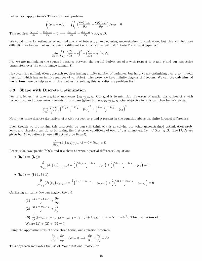
Let us now apply Green’s Theorem to our problem:∮L

(pdx+ qdy) =

∫∫D

(∂q(x, y)

∂x− ∂p(x, y)

∂y

)dxdy = 0

This requires ∂q(x,y)∂x − ∂p(x,y)

∂y = 0 =⇒ ∂q(x,y)∂x = ∂p(x,y)

∂y ∀ x, y ∈ D.

We could solve for estimates of our unknowns of interest, p and q, using unconstrained optimization, but this will be moredifficult than before. Let us try using a different tactic, which we will call “Brute Force Least Squares”:

minz(x,y)

∫∫D

(∂z∂x− p)2

+(∂z∂y− q)2

dxdy

I.e. we are minimizing the squared distance between the partial derivatives of z with respect to x and y and our respectiveparameters over the entire image domain D.

However, this minimization approach requires having a finite number of variables, but here we are optimizing over a continuousfunction (which has an infinite number of variables). Therefore, we have infinite degrees of freedom. We can use calculus ofvariations here to help us with this. Let us try solving this as a discrete problem first.

8.3 Shape with Discrete Optimization

For this, let us first take a grid of unknowns zij(i,j)∈D. Our goal is to minimize the errors of spatial derivatives of z withrespect to p and q, our measurements in this case (given by pij , qij(i,j)∈D. Our objective for this can then be written as:

minzij

∑i

∑j

(zi,j+1 − zi,jε

− pi,j)2

+(zi+1,j − zi,j

ε− qi,j

)2

Note that these discrete derivatives of z with respect to x and y present in the equation above use finite forward differences.

Even though we are solving this discretely, we can still think of this as solving our other unconstrained optimization prob-lems, and therefore can do so by taking the first-order conditions of each of our unknowns, i.e. ∀ (k, l) ∈ D. The FOCs aregiven by |D| equations (these will actually be linear!):

∂

∂zk,l(J(zi,j(i,j)∈D) = 0 ∀ (k, l) ∈ D

Let us take two specific FOCs and use them to write a partial differential equation:

• (k, l) = (i, j):

∂

∂zk,l(J(z,j(i,j)∈D) =

2

ε

(zk,l+1 − zk,lε

− pk,l)

+2

ε

(zk+1,l − zk,lε

− qk,l)

= 0

• (k, l) = (i+1, j+1):

∂

∂zk,l(J(z,j(i,j)∈D) =

2

ε

(zk,l − zk,l−1

ε− pk,l−1

)+

2

ε

(zk,l − zk−1,l

ε− qk−1,l

)= 0

Gathering all terms (we can neglect the zs):

(1)pk,l − pk,l−1

ε≈ ∂p

∂x

(2)qk,l − qk−1,l

ε≈ ∂q

∂y

(3)1

ε2((−zk,l+1 − zk+1,l − zk,l−1 − zk−1,l) + 4zk,l) = 0 ≈ −∆z = −∇2z The Laplacian of z

Where (1) + (2) + (3) = 0

Using the approximations of these three terms, our equation becomes:

∂p

∂x+∂q

∂y−∆z = 0 =⇒ ∂p

∂x+∂q

∂y= ∆z

This approach motivates the use of “computational molecules”.

48

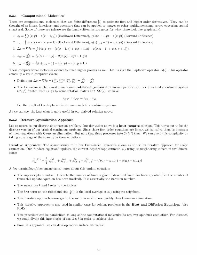
8.3.1 “Computational Molecules”

These are computational molecules that use finite differences [3] to estimate first and higher-order derivatives. They can bethought of as filters, functions, and operators that can be applied to images or other multidimensional arrays capturing spatialstructural. Some of these are (please see the handwritten lecture notes for what these look like graphically):

1. zx = 1ε (z(x, y)− z(x− 1, y)) (Backward Difference), 1

ε (z(x+ 1, y)− z(x, y)) (Forward Difference)

2. zy = 1ε (z(x, y)− z(x, y − 1)) (Backward Difference), 1

ε (z(x, y + 1)− z(x, y)) (Forward Difference)

3. ∆z = ∇2z = 1ε2 (4z(x, y)− (z(x− 1, y) + z(x+ 1, y) + z(x, y − 1) + z(x, y + 1)))

4. zxx = ∂2z∂x2 = 1

ε2 (z(x− 1, y)− 2(x, y) + z(x+ 1, y))

5. zyy = ∂2z∂y2 = 1

ε2 (z(x, y − 1)− 2(x, y) + z(x, y + 1))

These computational molecules extend to much higher powers as well. Let us visit the Laplacian operator ∆(·). This operatorcomes up a lot in computer vision:

• Definition: ∆z = ∇2z = ( ∂z∂x ,∂z∂y )T ( ∂z∂x ,

∂z∂y ) = ∂2z

∂x2 + ∂2z∂y2

• The Laplacian is the lowest dimensional rotationally-invariant linear operator, i.e. for a rotated coordinate system(x′, y′) rotated from (x, y) by some rotation matrix R ∈ SO(2), we have:

zx′x′ + zy′y′ = zxx + zyy

I.e. the result of the Laplacian is the same in both coordinate systems.

As we can see, the Laplacian is quite useful in our derived solution above.

8.3.2 Iterative Optimization Approach

Let us return to our discrete optimization problem. Our derivation above is a least-squares solution. This turns out to be thediscrete version of our original continuous problem. Since these first-order equations are linear, we can solve them as a systemof linear equations with Gaussian elimination. But note that these processes take O(N3) time. We can avoid this complexity bytaking advantage of the sparsity in these equations.

Iterative Approach: The sparse structure in our First-Order Equations allows us to use an iterative approach for shapeestimation. Our “update equation” updates the current depth/shape estimate zk,l using its neighboring indices in two dimen-sions:

z(n+1)k,l =

1

4(z

(n)k,l+1 + z

(n)k+1,l + z

(n)k,l−1 + z

(n)k−1,l)− ε(pk,l − pk,l−1)− ε(qk,l − qk−1,l)

A few terminology/phenomenological notes about this update equation:

• The superscripts n and n+ 1 denote the number of times a given indexed estimate has been updated (i.e. the number oftimes this update equation has been invoked). It is essentially the iteration number.

• The subscripts k and l refer to the indices.

• The first term on the righthand side 14 (·) is the local average of zk,l using its neighbors.

• This iterative approach converges to the solution much more quickly than Gaussian elimination.

• This iterative approach is also used in similar ways for solving problems in the Heat and Diffusion Equations (alsoPDEs).

• This procedure can be parallelized so long as the computational molecules do not overlap/touch each other. For instance,we could divide this into blocks of size 3 x 3 in order to achieve this.

• From this approach, we can develop robust surface estimates!

49

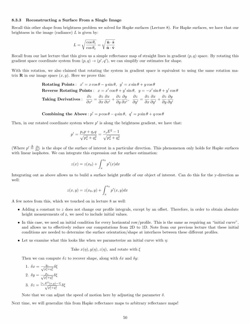
8.3.3 Reconstructing a Surface From a Single Image

Recall this other shape from brightness problem we solved for Hapke surfaces (Lecture 8). For Hapke surfaces, we have that ourbrightness in the image (radiance) L is given by:

L =

√cos θicos θe

=

√n · sn · v

Recall from our last lecture that this gives us a simple reflectance map of straight lines in gradient (p, q) space. By rotating thisgradient space coordinate system from (p, q)→ (p′, q′), we can simplify our estimates for shape.

With this rotation, we also claimed that rotating the system in gradient space is equivalent to using the same rotation ma-trix R in our image space (x, y). Here we prove this:

Rotating Points : x′ = x cos θ − y sin θ, y′ = x sin θ + y cos θ

Reverse Rotating Points : x = x′ cos θ + y′ sin θ, y = −x′ sin θ + y′ cos θ

Taking Derivatives :∂z

∂x′=∂z

∂x

∂x

∂x′+∂z

∂y

∂y

∂x′,∂z

∂y′=∂z

∂x

∂x

∂y′+∂z

∂y

∂y

∂y′

Combining the Above : p′ = p cos θ − q sin θ, q′ = p sin θ + q cos θ

Then, in our rotated coordinate system where p′ is along the brightness gradient, we have that:

p′ =psp+ qsq√p2s + q2

s

=rsE

2 − 1√p2s + q2

s

(Where p′∆= ∂z

∂x′ is the slope of the surface of interest in a particular direction. This phenomenon only holds for Hapke surfaceswith linear isophotes. We can integrate this expression out for surface estimation:

z(x) = z(x0) +

∫ x0

x

p′(x)dx

Integrating out as above allows us to build a surface height profile of our object of interest. Can do this for the y-direction aswell:

z(x, y) = z(x0, y) +

∫ x0

x

p′(x, y)dx

A few notes from this, which we touched on in lecture 8 as well:

• Adding a constant to z does not change our profile integrals, except by an offset. Therefore, in order to obtain absoluteheight measurements of z, we need to include initial values.

• In this case, we need an initial condition for every horizontal row/profile. This is the same as requiring an “initial curve”,and allows us to effectively reduce our computations from 2D to 1D. Note from our previous lecture that these initialconditions are needed to determine the surface orientation/shape at interfaces between these different profiles.

• Let us examine what this looks like when we parameterize an initial curve with η:

Take x(η), y(η), z(η), and rotate with ξ

Then we can compute δz to recover shape, along with δx and δy:

1. δx = qs√p2s+q

2s

δξ

2. δy = ps√p2s+q

2s

δξ

3. δz = [rsE2(x,y)−1]√p2s+q

2s

δξ

Note that we can adjust the speed of motion here by adjusting the parameter δ.

Next time, we will generalize this from Hapke reflectance maps to arbitrary reflectance maps!

50

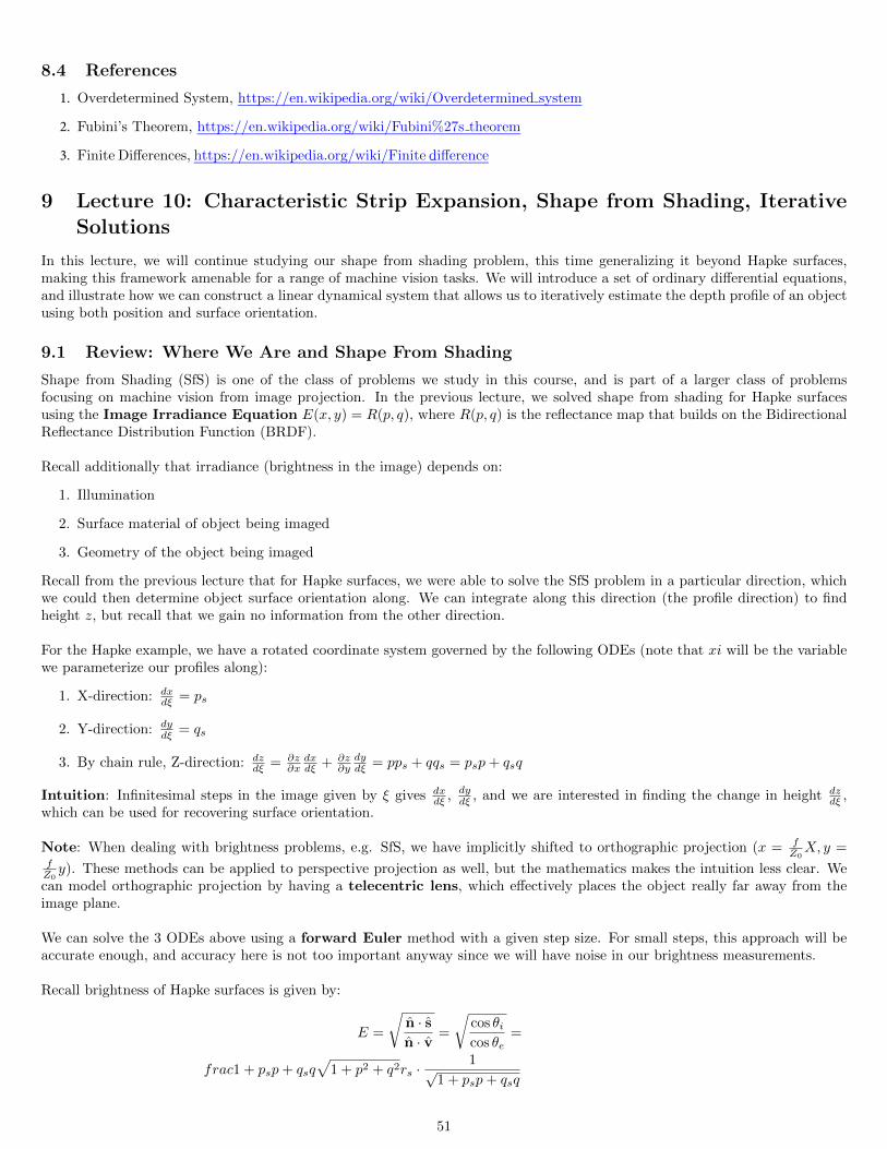
8.4 References

1. Overdetermined System, https://en.wikipedia.org/wiki/Overdetermined system

2. Fubini’s Theorem, https://en.wikipedia.org/wiki/Fubini%27s theorem

3. Finite Differences, https://en.wikipedia.org/wiki/Finite difference

9 Lecture 10: Characteristic Strip Expansion, Shape from Shading, IterativeSolutions

In this lecture, we will continue studying our shape from shading problem, this time generalizing it beyond Hapke surfaces,making this framework amenable for a range of machine vision tasks. We will introduce a set of ordinary differential equations,and illustrate how we can construct a linear dynamical system that allows us to iteratively estimate the depth profile of an objectusing both position and surface orientation.

9.1 Review: Where We Are and Shape From Shading

Shape from Shading (SfS) is one of the class of problems we study in this course, and is part of a larger class of problemsfocusing on machine vision from image projection. In the previous lecture, we solved shape from shading for Hapke surfacesusing the Image Irradiance Equation E(x, y) = R(p, q), where R(p, q) is the reflectance map that builds on the BidirectionalReflectance Distribution Function (BRDF).

Recall additionally that irradiance (brightness in the image) depends on:

1. Illumination

2. Surface material of object being imaged

3. Geometry of the object being imaged

Recall from the previous lecture that for Hapke surfaces, we were able to solve the SfS problem in a particular direction, whichwe could then determine object surface orientation along. We can integrate along this direction (the profile direction) to findheight z, but recall that we gain no information from the other direction.

For the Hapke example, we have a rotated coordinate system governed by the following ODEs (note that xi will be the variablewe parameterize our profiles along):

1. X-direction: dxdξ = ps

2. Y-direction: dydξ = qs

3. By chain rule, Z-direction: dzdξ = ∂z

∂xdxdξ + ∂z

∂ydydξ = pps + qqs = psp+ qsq

Intuition: Infinitesimal steps in the image given by ξ gives dxdξ , dy

dξ , and we are interested in finding the change in height dzdξ ,

which can be used for recovering surface orientation.

Note: When dealing with brightness problems, e.g. SfS, we have implicitly shifted to orthographic projection (x = fZ0X, y =

fZ0y). These methods can be applied to perspective projection as well, but the mathematics makes the intuition less clear. We

can model orthographic projection by having a telecentric lens, which effectively places the object really far away from theimage plane.

We can solve the 3 ODEs above using a forward Euler method with a given step size. For small steps, this approach will beaccurate enough, and accuracy here is not too important anyway since we will have noise in our brightness measurements.

Recall brightness of Hapke surfaces is given by:

E =

√n · sn · v

=

√cos θicos θe

=

frac1 + psp+ qsq√

1 + p2 + q2rs ·1√

1 + psp+ qsq

51

Some cancellation and rearranging yields:

psp+ qsq = rsE2 − 1

Therefore, we have a direct relationship between our measured brightness E and our unknowns of interest:

∂z

∂xps +

∂z

∂yqs = pps + qqs = rsE

2 − 1

Note here, however, that we do not know surface orientation based on this, since again for Hapke surfaces, we only know slopein one of our two directions in our rotated gradient space (p′, q′). A forward Euler approach will generate a set of independentprofiles, and we do not have any information about the surface orientation at the interfaces of these independent profiles. Thisnecessitates an initial curve containing initial conditions for each of these independent profiles. In 3D, this initial curve isparameterized by η, and is given by: (x(η), y(η), z(η)). Our goal is to find z(η, ξ), where:

• η parameterizes the length of the initial curve

• ξ parameterizes along the 1D profiles we carve out

Therefore, we are able to determine the slope in a particular direction.

9.2 General Case

Let us now generalize our Hapke case above to be any surface. We begin with our Image Irradiance Equation:

E(x, y) = R(p, q)

Let us now consider taking a small step δx, δy in the image, and our goal is to determine how z changes from this small step.We can do so using differentials and surface orientation:

δz =∂z

∂xδx+

∂z

∂yδy = pδx+ qδy

Therefore, if we know p and q, we can compute δz for a given δx and δy. But in addition to updating z using the equationabove, we will also need to update p and q (intuitively, since we are still moving, the surface orientation can change):

δp =∂p

∂xδx+

∂p

∂yδy

δq =∂q

∂xδx+

∂q

∂yδy

This notion of updating p and q provides motivation for keeping track/updating not only (x, y, z), but also p and q. We canthink of solving our problem as constructing a characteristic strip of the ODEs above, composed of (x, y, z, p, q) ∈ R5. Invector-matrix form, our updates to p and q become:

[δpδq

]=

r s

s t

[δxδy

]=

∂2z∂x2

∂2z∂y∂x

∂2z∂x∂y

∂2z∂y2

[δxδy]

=

px py

qx qy

[δxδy

]= H

[δxδy

]

Where H is the Hessian of second spatial derivatives (x and y) of z. Note that from Fubuni’s theorem and from our Taylorexpansion from last lecture, py = qx.

Intuition:

• First spatial derivatives ∂z∂x and ∂z

∂y describe the surface orientation of an oject in the image.

• Second spatial derivatives ∂2z∂x2 , ∂2z

∂y2 , and ∂2z∂x∂y = ∂2z

∂y∂x describe curvature, or the change in surface orientation.

• In 2D, the curvature of a surface is specified by the radius of curvature, or its inverse, curvature.

• In 3D, however, the curvature of a surface is specified by a Hessian matrix H. This curvature matrix allows us to computep and q.

52

One issue with using this Hessian approach to update p and q: how do we update the second derivatives r, s, and t? Can we use3rd order derivatives? It turns out that seeking to update lower-order derivatives with higher-order derivatives will just generateincreasingly more unknowns, so we will seek alternative routes. Let’s try integrating our brightness measurements into what wealready have so far:

Image Irradiance Equation : E(x, y) = R(p, q)

Chain Rule Gives :

Ex =∂E

∂x=∂R

∂p

∂p

∂x+∂R

∂q

∂q

∂x

=∂R

∂pr +

∂R

∂qs

Ey =∂E

∂y=∂R

∂p

∂p

∂y+∂R

∂q

∂q

∂y

=∂R

∂ps+

∂R

∂qt

In matrix-vector form, we have:

[ExEy

]=

[r ss t

]∂R∂p∂R∂q

= H

∂R∂p∂R∂q

Notice that we have the same Hessian matrix that we had derived for our surface orientation update equation before!

Intuition: These equations make sense intuitively - brightness will be constant for constant surface orientation in a modelwhere brightness depends only on surface orientation. Therefore, changes in brightness correspond to changes in surface orien-tation.

How do we solve for this Hessian H? We can:

• Solve for Ex, Ey numerically from our brightness measurements.

• Solve for Rp, Rq using our reflectance map.

However, solving for H in this way presents us with 3 unknowns and only 2 equations (undetermined system). We cannot solvefor H, but we can still compute δp, δq. We can pattern match δx and δy by using a (δx, δy)T vector in the same direction as thegradient of the reflectance map, i.e. [

δxδy

]=

[RpRq

]ξ

Where the vector on the lefthand side is our step in x and y, our vector on the righthand side is our gradient of the reflectancemap in gradient space (p, q), and ξ is the step size. Intuitively, this is the direction where we can “make progress”. Substitutingthis equality into our update equation for p and q, we have:[

δpδq

]= H

[RpRq

]ξ

=

[ExEy

]δξ

Therefore, we can formally write out a system of 5 first-order ordinary differential equations (ODEs) that generate our charac-teristic strip as desired:

1. dxdξ = Rp

2. dydξ = Rq

3. dpdξ = Ex

4. dqdξ = Ey

53

5. dzdξ = pRp + qRq (“Output Rule”)

Though we take partial derivatives on many of the righthand sides, we can think of these quantities as measurements or derivedvariations of our measurements, and therefore they do not correspond to partial derivatives that we actually need to solve for.Thus, this is why we claim this is a system of ODEs, and not PDEs.

A few notes about this system of ODEs:

• This system of 5 ODEs explores the surface along the characteristic strip generated by these equations.

• Algorithmically, we (a) Look at/compute the brightness gradient, which helps us (b) Compute p and q, which (c) Informsus of Rp and Rq for computing the change in height z.

• ODEs 1 & 2 and ODEs 3 & 4 are two systems of equations that each determine the update for the other system (i.e. thereis dynamic behavior between these two systems). The 5th ODE is in turn updated from the results of updating the other4 ODE quantities of interest.

• The step in the image (x,y) depends on the gradient of the reflectance map in (p,q).

• Analogously, the step in the reflectance map (p,q) depends on the gradient of the image in (x,y).

• This system of equations necessitates that we cannot simply optimize with block gradient ascent or descent, but rather aprocess in which we dynamically update our variables of interest using our other updated variables of interest.

• This approach holds generally for any reflectance map R(p, q).

• We can express our image irradiance equation as a first order, nonlinear PDE:

E(x, y) = R(∂z∂x,∂z

∂y

)Next, we will show how this general approach applied to a Hapke surface reduces to our previous SfS results for this problem.

9.2.1 Reducing General Form SfS for Hapke Surfaces

Recall reflectance map for Hapke surfaces:

R(p, q) =

√1 + psp+ qsq

rs

Taking derivatives using the system of 5 ODEs defined above, we have from the multivariate chain rule):

1. dxdξ : Rp

∆= ∂R

∂p = 1√rs

12√

1+psp+qsqps

2. dydξ : Rq

∆= ∂R

∂q = 1√rs

12√

1+psp+qsqqs

3. dzdξ : pRp + qRq = psp+qsq

2√rs√

1+psp+qsq

Since the denominator is common in all three of these derivative equations, we can just conceptualize this factor as a speed/stepsize factor. Therefore, we can simply omit this factor when we update these variables after taking a step. With this, our updatesbecome:

1. δx← ps

2. δy ← qs

3. δz ← (psp+ qsq) = rsE2 − 1

Which are consistent with our prior results using our Hapke surfaces. Next, we will apply this generalized approach to ScanningElectron Microscopes (SEMs):

54

9.2.2 Applying General Form SfS to SEMs

For SEMs, the reflectance map is spherically symmetric around the origin:

R(p, q) = f(p2 + q2) for some f : R → R

Using our system of 5 ODEs derived in the general case, we can compute our updates by first calculating derivatives dxdξ , dydξ , and

dzdξ :

1. dxdξ : Rp

∆= ∂R

∂p = 2f ′(p2 + q2)p

2. dydξ : Rq

∆= ∂R

∂q = 2f ′(p2 + q2)q

3. dzdξ : pRp + qRq = 2f ′(p2 + q2)(p2 + q2)

Again, here we can also simplify these updates by noting that the term 2f ′(p2 + q2) is common to all three derivatives, andtherefore this factor can also be interpreted as a speed factor that only affects the step size. Our updates then become:

1. δx← p

2. δy ← q

3. δz ← p2 + q2

This tells us we will be taking steps along the brightness gradient. Our solution generates characteristic strips that containinformation about the surface orientation. To continue our analysis of this SfS problem, in addition to defining characteristicstrips, it will also be necessary to define the base characteristic.

9.3 Base Characteristics

Recall that the characteristic strip that our system of ODEs solves for is given by a 5-dimensional surface composed of:[x y z p q

]T ∈ R5

Another important component when discussing our solution to this SfS problem is the base characteristic, which is theprojection of the characteristic strip onto the x, y image plane:[

x(ξ) y(ξ)]T

= projectionx,ycharacteristic strip = projectionx,y[x y z p q

]T A few notes/questions about base characteristics?

• What are base characteristics? These can be thought of as the profiles in the (x, y) plane that originate (possibly inboth directions) from a given point in the initial curve.

• What are base characteristics used for? These are used to help ensure we explore as much of the image as possible.We can interpolate/average (depending on how dense/sparse a given region of the image is) different base characteristicsto “fill out” the solution over the entire image space.

• How are base characteristics used in practice? Like the solution profiles we have encountered before, base charac-teristics are independent of one another - this allows computation over them to be parallelizable. Intuition: These setsof base characteristics can be thought of like a wavefront propagating outward from the initial curve. We expect thesolutions corresponding to these base characteristics to move at similar “speeds”.

9.4 Analyzing “Speed”

When considering how the speeds of these different solution curves vary, let us consider ways in which we can set constant stepsizes/speeds. Here are a few, to name:

1. Constant step size in z: This is effectively stepping “contour to contour” on a topographic map.Achieved by: Dividing by pRp + qRq =⇒ dz

dξ = 1.

2. Constant step size in image: A few issues with this approach. First, curves may run at different rates. Second,

methodology fails when√R2p +R2

q = 0.

Achieved by: Dividing by√R2p +R2

q =⇒ ddξ (√δx2 + δy2) = 1.

55

3. Constant Step Size in 3D/Object: Runs into issues when Rp = Rq = 0.

Achieved by: Dividing by√R2p +R2

q + (pRp + qRq)2 =⇒√

(δx)2 + (δy)2 + (δz)2 = 1.

4. Constant Step Size in Isophotes: Here, we are effectively taking constant steps in brightness. We will end up dividingby the dot product of the brightness gradient and the gradient of the reflectance map in (p, q) space.Achieved by: Dividing by (∂E∂x

∂R∂p + ∂E

∂y∂R∂q )δξ = ((Ex, Ey) · (Rp, Rq))δξ =⇒ δE = 1.

9.5 Generating an Initial Curve

While only having to measure a single initial curve for profiling is far better than having to measure an entire surface, it is stillundesirable and is not a caveat we are satisfied with for this solution. Below, we will discuss how we can generate an initialcurve to avoid having to measure one for our SfS problem.

As we discussed, it is undesirable to have to measure an initial curve/characteristic strip, a.k.a. measure:[x(ξ) y(ξ) z(ξ) p(ξ) q(ξ)

]TBut we do not actually need to measure all of these. Using the image irradiance equation we can calculate ∂z

∂η :

E(x, y) = R(p, q)

∂z

∂η=∂z

∂x

∂x

∂η+∂z

∂y

∂y

∂η

= p∂x

∂η+ q

∂y

∂η

Where p and q in this case are our unknowns. Therefore, in practice, we can get by with just initial curve, and do not need thefull initial characteristic strip - i.e. if we have x(η), y(η), and z(η), then we can compute the orientation from the reflectancemap using our brightness measurements.

9.5.1 Using Edge Points to Autogenerate an Initial Curve

An even more sweeping question: do we even need an initial curve? Are there any special points on the object where we alreadyknow the orientation without a measurement? These points are along the edge, or occluding boundary, of our objects ofinterest. Here, we know the surface normal of each of these points. Could we use these edge points as “starting points” for ourSfS solution?

It turns out, unfortunately, that we cannot. This is due to the fact that as we infinisimally approach the edge of the boundary,

we have that∣∣∣ ∂z∂x ∣∣∣ → ∞, ∣∣∣ ∂z∂y ∣∣∣ → ∞. Even though the slope q

p is known, we cannot use it numerically/iteratively with our step

updates above.

9.5.2 Using Stationary Points to Autogenerate an Initial Curve

Let us investigate another option for helping us to avoid having to generate an initial curve. Consider the brightest (or darkest)point on an image, i.e. the unique, global, isolated extremum. This point is a stationary point in (p, q) space, i.e.

∂R

∂p=∂R

∂q= 0, granted that R(p, q) is differentiable.

This would allow us to find the surface orientation (p, q) solely through optimizing the reflectance map function R(p, q). Oneimmediate problem with this stationary point approach is that we will not be able to step x and y, since, from our system ofODEs, we have that at our stationary points, our derivatives of x and y are zero:

dx

dξ= Rp = 0

dy

dξ= Rq = 0

Additionally, if we have stationary brightness points in image space, we encounter the “dual” of this problem. By definitionstationary points in the image space imply that:

∂E

∂x=∂E

∂y= 0

56

This in turn implies that p and q cannot be stepped:

dp

dξ=∂E

∂x= 0

dq

dξ=∂E

∂y= 0

Intuition: Intuitively, what is happening with these two systems (each of 2 ODEs ((x, y) or p, q), as we saw in our 5 ODEsystem above) is that using stationary points in one domain amounts to updates in the other domain going to zero, which in turnprevents the other system’s quantities of interest from stepping. Since δz depends on δx, δy, δp, δq, and since δx, δy, δp, δq = 0when we use stationary points as starting points, this means we cannot ascertain any changes in δz along these points.

Note: The extremum corresponding to a stationary point can be maximum, as it is for Lambertian surfaces, or a mini-mum, as it is for Scanning Electron Microscopes (SEM).

However, even though we cannot use stationary points themselves as starting points, could we use the area around them?If we stay close enough to the stationary point, we can approximate that these neighboring points have nearly the same surfaceorientation.

• Approach 1: Construct a local tangent plane by extruding a circle in the plane centered at the stationary point withradius ε - this means all points in this plane will have the same surface orientation as the stationary point. Note thatmathematically, a local 2D plane on a 3D surface is equivalent to a 2-manifold [1]. This is good in the sense that we knowthe surface orientation of all these points already, but not so great in that we have a degenerate system - since all pointshave the same surface orientation, under this model they will all have the same brightness as well. This prevents us fromobtaining a unique solution.

• Approach 2: Rather than constructing a local planar surface, let us take a curved surface with non-constant surfaceorientation and therefore, under this model, non-constant brightness.

9.5.3 Example

Suppose we have a reflectance map and surface function given by:

Reflectance Map : R(p, q) = p2 + q2

Surface Function : z(x, y) = x2 + y2

Then, we can compute the derivatives of these as:

p =∂z

∂x= 2x

q =∂z

∂y= 4y

E(x, y) = R(p, q) = p2 + q2 = 4x2 + 16y2

Ex =∂E

∂x= 8x

Ey =∂E

∂y= 32y

The brightness gradient (∂E∂x ,∂E∂y ) = (8x, 32y) = (0, 0) at the origin x = 0, y = 0.

Can we use the brightness gradient to estimate local shape? It turns out the answer is no, again because of stationary points.But if we look at the second derivatives of brightness:

Exx =∂2E

∂x2=∂E

∂x(8x) = 8

Eyy =∂2E

∂y2=∂E

∂y(32y) = 32

Exy =∂2E

∂x∂y=

∂

∂x(32y) =

∂

∂y(8y) = 0

57

These second derivatives, as we will discuss more in the next lecture, will tell us some information about the object’s shape.As we have seen in previous lectures, these second derivatives can be computed by applying computational molecules to ourbrightness measurements.

High-Level Algorithm

(NOTE: This will be covered in greater detail next lecture) Let’s walk through the steps to ensure we can autogenerate aninitial condition curve without the need to measure it:

1. Compute stationary points of brightness.

2. Use 2nd derivatives of brightness to estimate local shape.

3. Construct small cap (non-planar to avoid degeneracy) around the stationary point.

4. Begin solutions from these points on the edge of the cap surrounding the stationary point.

9.6 References

1. Manifold, https://en.wikipedia.org/wiki/Manifold

10 Lecture 11: Edge Detection, Subpixel Position, CORDIC, Line Detection,(US 6,408,109)

In this lecture, we will introduce some discussion on how patents work, their stipulations, and make our discussion explicit bylooking at a patent case study with sub-pixel accuracy edge detection. You can find the patent document on Stellar as wellunder “Materials” → “US patent 6,408,109”.

10.1 Background on Patents

We will begin with some fun facts about industrial machine vision:

• Integrated circuit boards cannot be manufactured without machine vision

• Pharmaceutical chemicals also cannot be manufactured without machine vision

How do entrepreneurs and industrial companies ensure their inventions are protected, while still having the chance to disseminatetheir findings with society? This si done through patents. Patents:

• Can be thought of as a “contract with society” - you get a limited monopoly on your idea, and in turn, you publish thetechnical details of your approach.

• Can help to reduce litigation and legal fees.

• Can be used by large companies as “ammunition” for “patent wars”.

Some “rules” of patents:

• No equations are included in the patent (no longer true)

• No greyscale images - only black and white

• Arcane grammar is used for legal purposes - “comprises”, “apparatus”, “method”, etc.

• References of other patents are often included - sometimes these are added by the patent examiner, rather than the patentauthors

• Most patents end with something along the lines of “this is why our invention was necessary” or “this is the technical gapour invention fills”

• Software is not patentable - companies and engineers get around this by putting code on hardware and patenting the“apparatus” housing the code.

• It is also common to include background information (similar to related literature in research).

Now that we have had a high-level introduction to patents, let us turn to focus on one that describes an apparatus for sub-pixelaccuracy edge finding.

58

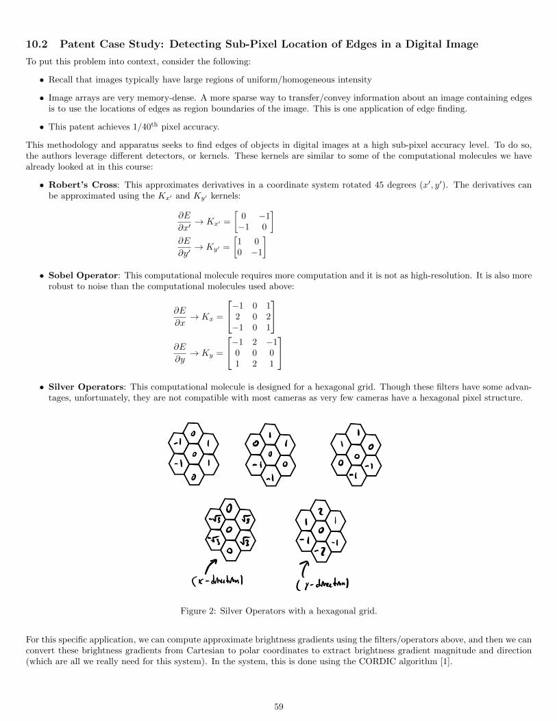
10.2 Patent Case Study: Detecting Sub-Pixel Location of Edges in a Digital Image

To put this problem into context, consider the following:

• Recall that images typically have large regions of uniform/homogeneous intensity

• Image arrays are very memory-dense. A more sparse way to transfer/convey information about an image containing edgesis to use the locations of edges as region boundaries of the image. This is one application of edge finding.

• This patent achieves 1/40th pixel accuracy.

This methodology and apparatus seeks to find edges of objects in digital images at a high sub-pixel accuracy level. To do so,the authors leverage different detectors, or kernels. These kernels are similar to some of the computational molecules we havealready looked at in this course:

• Robert’s Cross: This approximates derivatives in a coordinate system rotated 45 degrees (x′, y′). The derivatives canbe approximated using the Kx′ and Ky′ kernels:

∂E

∂x′→ Kx′ =

[0 −1−1 0

]∂E

∂y′→ Ky′ =

[1 00 −1

]• Sobel Operator: This computational molecule requires more computation and it is not as high-resolution. It is also more

robust to noise than the computational molecules used above:

∂E

∂x→ Kx =

−1 0 12 0 2−1 0 1

∂E

∂y→ Ky =

−1 2 −10 0 01 2 1

• Silver Operators: This computational molecule is designed for a hexagonal grid. Though these filters have some advan-

tages, unfortunately, they are not compatible with most cameras as very few cameras have a hexagonal pixel structure.

Figure 2: Silver Operators with a hexagonal grid.

For this specific application, we can compute approximate brightness gradients using the filters/operators above, and then we canconvert these brightness gradients from Cartesian to polar coordinates to extract brightness gradient magnitude and direction(which are all we really need for this system). In the system, this is done using the CORDIC algorithm [1].

59

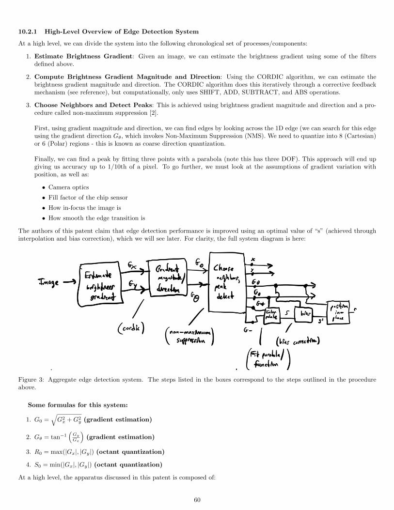
10.2.1 High-Level Overview of Edge Detection System

At a high level, we can divide the system into the following chronological set of processes/components:

1. Estimate Brightness Gradient: Given an image, we can estimate the brightness gradient using some of the filtersdefined above.

2. Compute Brightness Gradient Magnitude and Direction: Using the CORDIC algorithm, we can estimate thebrightness gradient magnitude and direction. The CORDIC algorithm does this iteratively through a corrective feedbackmechanism (see reference), but computationally, only uses SHIFT, ADD, SUBTRACT, and ABS operations.

3. Choose Neighbors and Detect Peaks: This is achieved using brightness gradient magnitude and direction and a pro-cedure called non-maximum suppression [2].

First, using gradient magnitude and direction, we can find edges by looking across the 1D edge (we can search for this edgeusing the gradient direction Gθ, which invokes Non-Maximum Suppression (NMS). We need to quantize into 8 (Cartesian)or 6 (Polar) regions - this is known as coarse direction quantization.

Finally, we can find a peak by fitting three points with a parabola (note this has three DOF). This approach will end upgiving us accuracy up to 1/10th of a pixel. To go further, we must look at the assumptions of gradient variation withposition, as well as:

• Camera optics

• Fill factor of the chip sensor

• How in-focus the image is

• How smooth the edge transition is

The authors of this patent claim that edge detection performance is improved using an optimal value of “s” (achieved throughinterpolation and bias correction), which we will see later. For clarity, the full system diagram is here:

Figure 3: Aggregate edge detection system. The steps listed in the boxes correspond to the steps outlined in the procedureabove.

Some formulas for this system:

1. G0 =√G2x +G2

y (gradient estimation)

2. Gθ = tan−1(GyGx

)(gradient estimation)

3. R0 = max(|Gx|, |Gy|) (octant quantization)

4. S0 = min(|Gx|, |Gy|) (octant quantization)

At a high level, the apparatus discussed in this patent is composed of:

60

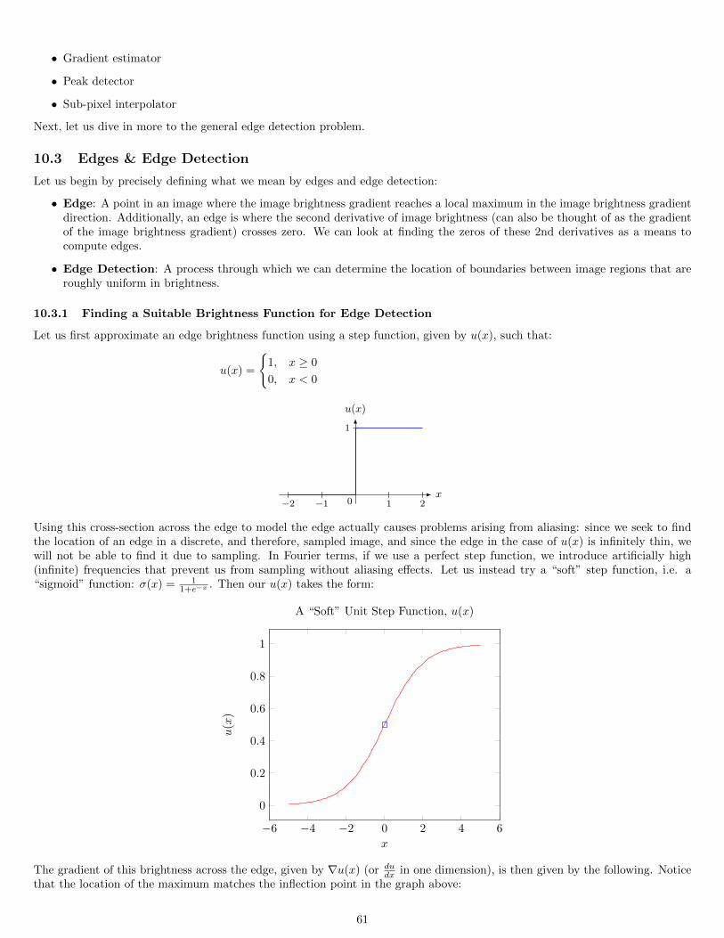
• Gradient estimator

• Peak detector

• Sub-pixel interpolator

Next, let us dive in more to the general edge detection problem.

10.3 Edges & Edge Detection

Let us begin by precisely defining what we mean by edges and edge detection:

• Edge: A point in an image where the image brightness gradient reaches a local maximum in the image brightness gradientdirection. Additionally, an edge is where the second derivative of image brightness (can also be thought of as the gradientof the image brightness gradient) crosses zero. We can look at finding the zeros of these 2nd derivatives as a means tocompute edges.

• Edge Detection: A process through which we can determine the location of boundaries between image regions that areroughly uniform in brightness.

10.3.1 Finding a Suitable Brightness Function for Edge Detection

Let us first approximate an edge brightness function using a step function, given by u(x), such that:

u(x) =

1, x ≥ 0

0, x < 0

−2 −1 1 20

1

x

u(x)

Using this cross-section across the edge to model the edge actually causes problems arising from aliasing: since we seek to findthe location of an edge in a discrete, and therefore, sampled image, and since the edge in the case of u(x) is infinitely thin, wewill not be able to find it due to sampling. In Fourier terms, if we use a perfect step function, we introduce artificially high(infinite) frequencies that prevent us from sampling without aliasing effects. Let us instead try a “soft” step function, i.e. a“sigmoid” function: σ(x) = 1

1+e−x . Then our u(x) takes the form:

−6 −4 −2 0 2 4 6

0

0.2

0.4

0.6

0.8

1

x

u(x

)

A “Soft” Unit Step Function, u(x)

The gradient of this brightness across the edge, given by ∇u(x) (or dudx in one dimension), is then given by the following. Notice

that the location of the maximum matches the inflection point in the graph above:

61

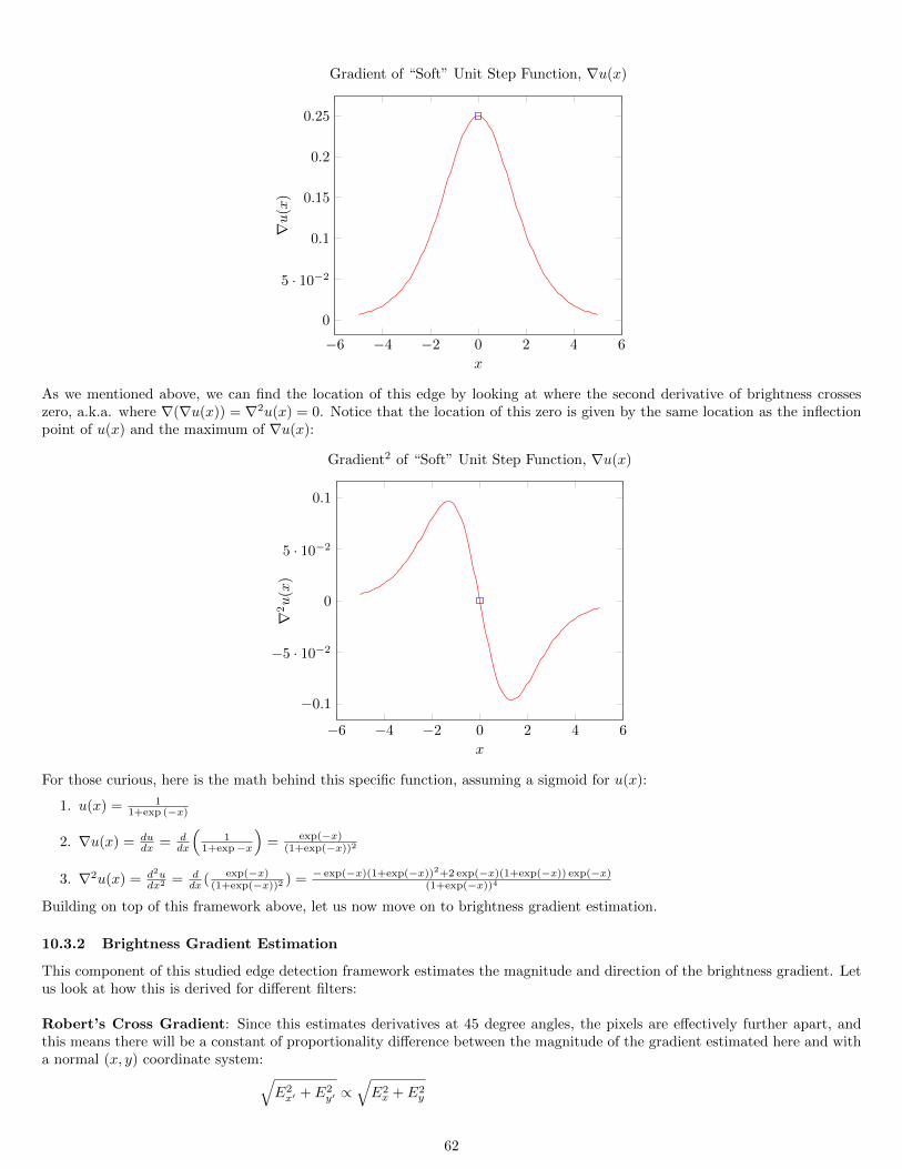
−6 −4 −2 0 2 4 6

0

5 · 10−2

0.1

0.15

0.2

0.25

x

∇u

(x)

Gradient of “Soft” Unit Step Function, ∇u(x)

As we mentioned above, we can find the location of this edge by looking at where the second derivative of brightness crosseszero, a.k.a. where ∇(∇u(x)) = ∇2u(x) = 0. Notice that the location of this zero is given by the same location as the inflectionpoint of u(x) and the maximum of ∇u(x):

−6 −4 −2 0 2 4 6

−0.1

−5 · 10−2

0

5 · 10−2

0.1

x

∇2u

(x)

Gradient2 of “Soft” Unit Step Function, ∇u(x)

For those curious, here is the math behind this specific function, assuming a sigmoid for u(x):

1. u(x) = 11+exp (−x)

2. ∇u(x) = dudx = d

dx

(1

1+exp−x

)= exp(−x)

(1+exp(−x))2

3. ∇2u(x) = d2udx2 = d

dx ( exp(−x)(1+exp(−x))2 ) = − exp(−x)(1+exp(−x))2+2 exp(−x)(1+exp(−x)) exp(−x)

(1+exp(−x))4

Building on top of this framework above, let us now move on to brightness gradient estimation.

10.3.2 Brightness Gradient Estimation

This component of this studied edge detection framework estimates the magnitude and direction of the brightness gradient. Letus look at how this is derived for different filters:

Robert’s Cross Gradient: Since this estimates derivatives at 45 degree angles, the pixels are effectively further apart, andthis means there will be a constant of proportionality difference between the magnitude of the gradient estimated here and witha normal (x, y) coordinate system:√

E2x′ + E2

y′ ∝√E2x + E2

y

62

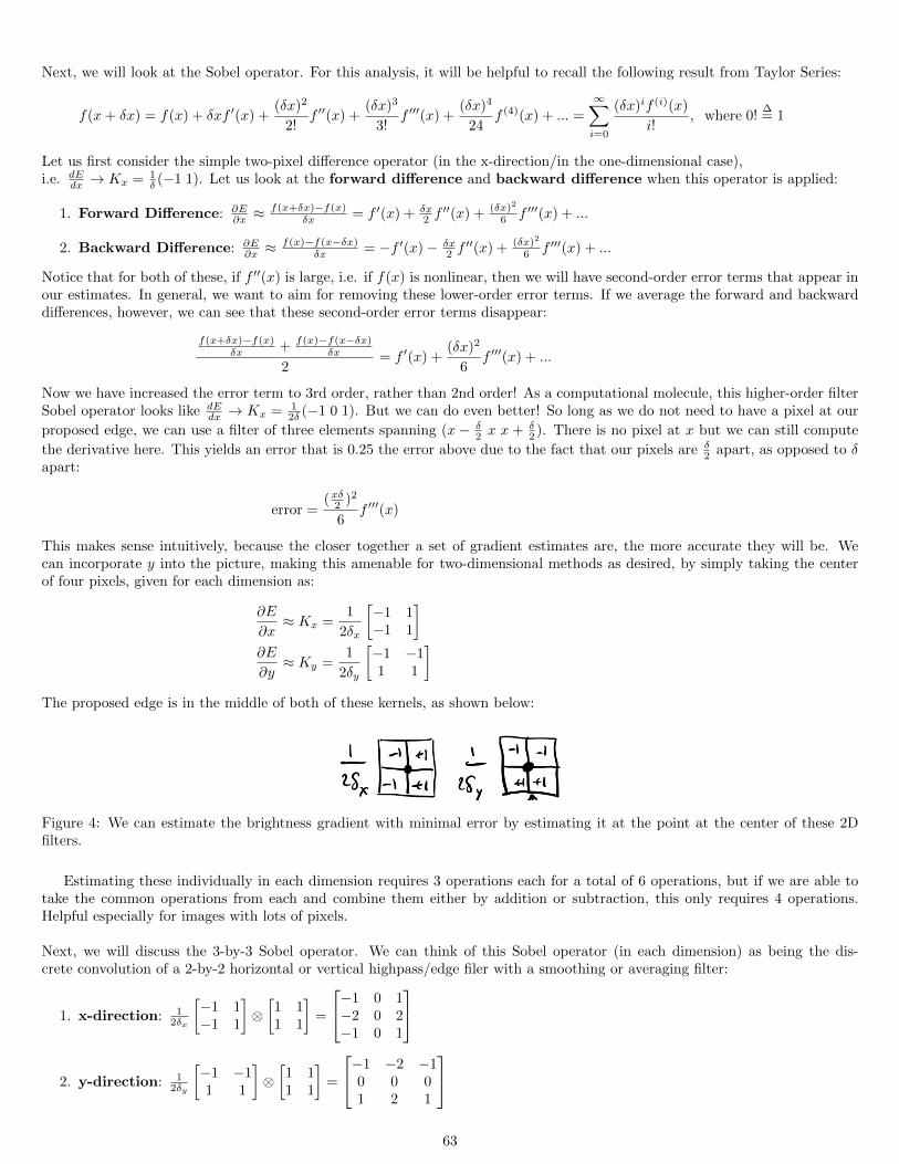
Next, we will look at the Sobel operator. For this analysis, it will be helpful to recall the following result from Taylor Series:

f(x+ δx) = f(x) + δxf ′(x) +(δx)2

2!f ′′(x) +

(δx)3

3!f ′′′(x) +

(δx)4

24f (4)(x) + ... =

∞∑i=0

(δx)if (i)(x)

i!, where 0!

∆= 1

Let us first consider the simple two-pixel difference operator (in the x-direction/in the one-dimensional case),i.e. dE

dx → Kx = 1δ (−1 1). Let us look at the forward difference and backward difference when this operator is applied:

1. Forward Difference: ∂E∂x ≈

f(x+δx)−f(x)δx = f ′(x) + δx

2 f′′(x) + (δx)2

6 f ′′′(x) + ...

2. Backward Difference: ∂E∂x ≈

f(x)−f(x−δx)δx = −f ′(x)− δx

2 f′′(x) + (δx)2

6 f ′′′(x) + ...

Notice that for both of these, if f ′′(x) is large, i.e. if f(x) is nonlinear, then we will have second-order error terms that appear inour estimates. In general, we want to aim for removing these lower-order error terms. If we average the forward and backwarddifferences, however, we can see that these second-order error terms disappear:

f(x+δx)−f(x)δx + f(x)−f(x−δx)

δx

2= f ′(x) +

(δx)2

6f ′′′(x) + ...

Now we have increased the error term to 3rd order, rather than 2nd order! As a computational molecule, this higher-order filterSobel operator looks like dE

dx → Kx = 12δ (−1 0 1). But we can do even better! So long as we do not need to have a pixel at our

proposed edge, we can use a filter of three elements spanning (x − δ2 x x + δ

2 ). There is no pixel at x but we can still compute

the derivative here. This yields an error that is 0.25 the error above due to the fact that our pixels are δ2 apart, as opposed to δ

apart:

error =(xδ2 )2

6f ′′′(x)

This makes sense intuitively, because the closer together a set of gradient estimates are, the more accurate they will be. Wecan incorporate y into the picture, making this amenable for two-dimensional methods as desired, by simply taking the centerof four pixels, given for each dimension as:

∂E

∂x≈ Kx =

1

2δx

[−1 1−1 1

]∂E

∂y≈ Ky =

1

2δy

[−1 −11 1

]The proposed edge is in the middle of both of these kernels, as shown below:

Figure 4: We can estimate the brightness gradient with minimal error by estimating it at the point at the center of these 2Dfilters.

Estimating these individually in each dimension requires 3 operations each for a total of 6 operations, but if we are able totake the common operations from each and combine them either by addition or subtraction, this only requires 4 operations.Helpful especially for images with lots of pixels.

Next, we will discuss the 3-by-3 Sobel operator. We can think of this Sobel operator (in each dimension) as being the dis-crete convolution of a 2-by-2 horizontal or vertical highpass/edge filer with a smoothing or averaging filter:

1. x-direction: 12δx

[−1 1−1 1

]⊗[1 11 1

]=

−1 0 1−2 0 2−1 0 1

2. y-direction: 12δy

[−1 −11 1

]⊗[1 11 1

]=

−1 −2 −10 0 01 2 1

63

A few notes about the derivation above:

• The convolution used is a “padded convolution” [3], in which, when implemented, when the elements of the filter/kernel(in this case, the averaging kernel) are not aligned with the image, they are simply multiplied by zero. Zero padding is themost common padding technique, but there are other techniques as well, such as wraparound padding.

• This approach avoids the half-pixel (in which we estimate an edge that is not on a pixel) that was cited above.

• Smoothing/averaging is a double edge sword, because while it can reduce/remove high-frequency noise by filtering, it canalso introduce undesirable blurring.

Next, we will look at how the brightness gradient is converted from Cartesian to Polar coordinates:

(Ex, Ey)→ (E0, Eθ)

E0 =√E2x + E2

y

Eθ = tan−1(EyEy

)Finally, we conclude this lecture by looking at appropriate values of s for quadratic and triangular functions. This assumes wehave three gradient measurements centered on G0: (1) G−, (2) G0, and (3) G+. Let us look at the results for these two typesof functions:

1. Quadratic: s = G+−G−4(G0− 1

2 (G+−G−)), this results in s ∈ [− 1

2 ,12 ].

2. Triangular: s = G+−G−2(G0−min(G+,G−))

A few notes about these approaches:

• Note that in each case, we only want to keep if the magnitude G0 is a local maximum, i.e. G0 > G+ and G0 ≥ G−.

• In the quadratic case, we can parameterize the curve with three data points using three degrees of freedom, i.e. ax2+bx+c =0. With this approach, b ≈ first derivative and a ≈ second derivative.

10.4 References

1. CORDIC Algorithm, https://www.allaboutcircuits.com/technical-articles/an-introduction-to-the-cordic-algorithm/

2. Non-Maximum Supression, http://justin-liang.com/tutorials/canny/#suppression

3. Padded Convolution, https://medium.com/@ayeshmanthaperera/what-is-padding-in-cnns-71b21fb0dd7

11 Lecture 12: Blob analysis, Binary Image Processing, Use of Green’s The-orem, Derivative and Integral as Convolutions

In this lecture, we will continue our discussion of intellectual property, and how it relevant for all scientists and engineers. Wewill then elaborate on some of the specific machine vision techniques that were used in this patent, as well as introduce somepossible extensions that could be applicable for this patent as well.

11.1 Types of Intellectual Property

Though it is not related to the technical content of machine vision, being familiar with different types and degrees of intellectualproperty (IP) is crucial to professional success. Below, we discuss some of these different types of intellectual property.

• Patents: One major type of these is utility and design patents. In these, the authors are required to disclose the “bestmode” of performance. For convenience, here are some notes on patents from our previous lecture:

– Can be thought of as a “contract with society” - you get a limited monopoly on your idea, and in turn, you publishthe technical details of your approach.

– Can help to reduce litigation and legal fees.

– Can be used by large companies as “ammunition” for “patent wars”.

64

Some “rules” of patents:

– No equations are included in the patent (no longer true)

– No greyscale images - only black and white

– Arcane grammar is used for legal purposes - “comprises”, “apparatus”, “method”, etc.

– References of other patents are often included - sometimes these are added by the patent examiner, rather than thepatent authors

– Most patents end with something along the lines of “this is why our invention was necessary” or “this is the technicalgap our invention fills”

– Software is not patentable - companies and engineers get around this by putting code on hardware and patenting the“apparatus” housing the code.

– It is also common to include background information (similar to related literature in research).

• Copyright:

– Books, song recordings, choreographs

– Exceptions: presenting (fractional pieces of) information from another author

• Trademarks:

– Must be unique for your field (e.g. Apple vs. Apple).

– Cannot use common words - this is actually one reason why many companies have slightly misspelled combinationsof common words.

– Can use pictures, character distortions, and color as part of the trademark.

– No issues if in different fields.

• Trade Secret

– No protections, but not spilled, lasts forever

– Can enforce legal recourse with Non-Disclosure Agreement (NDA)

11.2 Edge Detection Patent Methodologies

For this next section, we will direct our attention toward covering concepts that were discussed in the edge detection patent(6,408,109). Each of these sections will be discussed in further detail below. Before we get into the specifics of the patent again,it is important to point out the importance of edge detection for higher-level machine vision tasks, such as:

• Attitude (pose estimation) of an object

• Object recognition

• Determining to position

We will touch more on these topics in later lectures.

11.2.1 Finding Edge with Derivatives

Recall that we find a proposed edge by finding an inflection point of the brightness E(x, y). The following methods for findingthis point are equivalent:

• Finding an inflection point of brightness E(x, y).

• Finding maximum of brightness gradient magnitude/first derivative |∇E(x, y)|.

• Finding zero crossing of Laplacian/second derivative ∇2E(x, y).

For building intuition, last time we used the following example of u(x) = σ(x) = 11+exp(−x) :

65

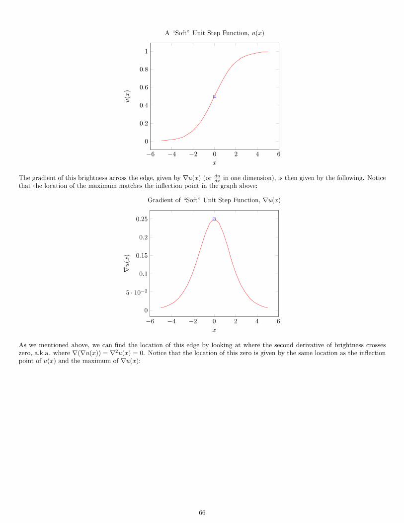
−6 −4 −2 0 2 4 6

0

0.2

0.4

0.6

0.8

1

x

u(x

)

A “Soft” Unit Step Function, u(x)

The gradient of this brightness across the edge, given by ∇u(x) (or dudx in one dimension), is then given by the following. Notice

that the location of the maximum matches the inflection point in the graph above:

−6 −4 −2 0 2 4 6

0

5 · 10−2

0.1

0.15

0.2

0.25

x

∇u

(x)

Gradient of “Soft” Unit Step Function, ∇u(x)

As we mentioned above, we can find the location of this edge by looking at where the second derivative of brightness crosseszero, a.k.a. where ∇(∇u(x)) = ∇2u(x) = 0. Notice that the location of this zero is given by the same location as the inflectionpoint of u(x) and the maximum of ∇u(x):

66

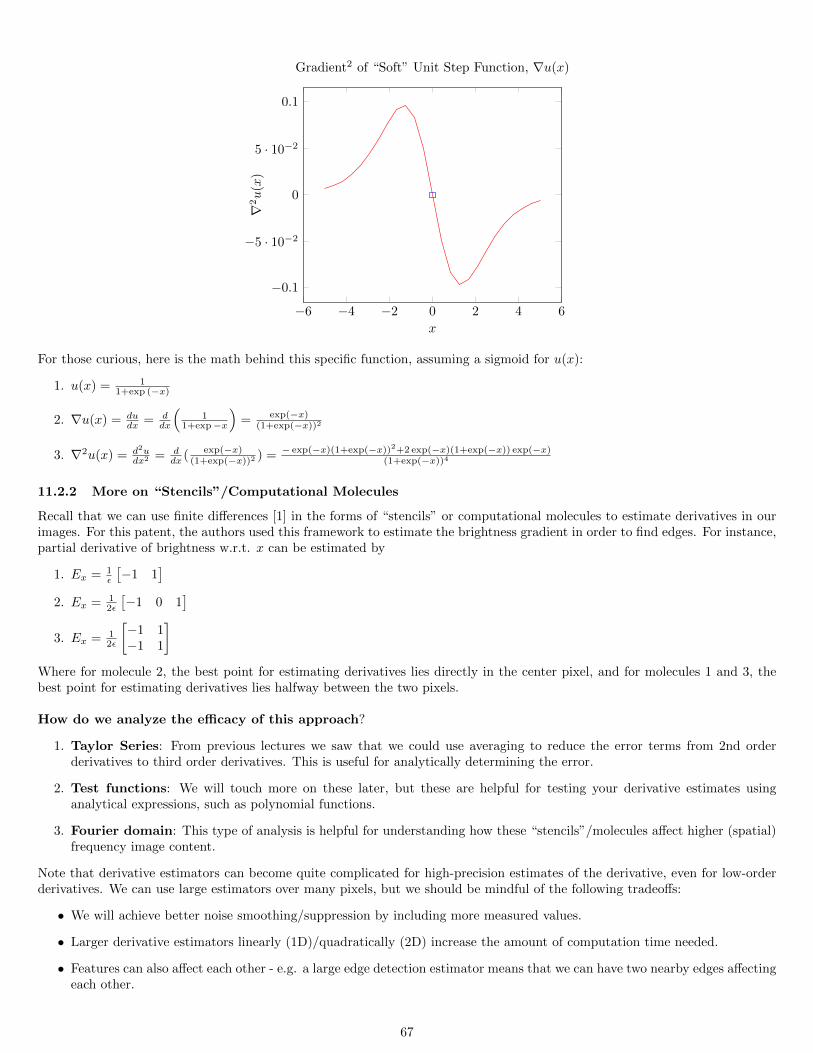
−6 −4 −2 0 2 4 6

−0.1

−5 · 10−2

0

5 · 10−2

0.1

x

∇2u

(x)

Gradient2 of “Soft” Unit Step Function, ∇u(x)

For those curious, here is the math behind this specific function, assuming a sigmoid for u(x):

1. u(x) = 11+exp (−x)

2. ∇u(x) = dudx = d

dx

(1

1+exp−x

)= exp(−x)

(1+exp(−x))2

3. ∇2u(x) = d2udx2 = d

dx ( exp(−x)(1+exp(−x))2 ) = − exp(−x)(1+exp(−x))2+2 exp(−x)(1+exp(−x)) exp(−x)

(1+exp(−x))4

11.2.2 More on “Stencils”/Computational Molecules

Recall that we can use finite differences [1] in the forms of “stencils” or computational molecules to estimate derivatives in ourimages. For this patent, the authors used this framework to estimate the brightness gradient in order to find edges. For instance,partial derivative of brightness w.r.t. x can be estimated by

1. Ex = 1ε

[−1 1

]2. Ex = 1

2ε

[−1 0 1

]3. Ex = 1

2ε

[−1 1−1 1

]Where for molecule 2, the best point for estimating derivatives lies directly in the center pixel, and for molecules 1 and 3, thebest point for estimating derivatives lies halfway between the two pixels.

How do we analyze the efficacy of this approach?

1. Taylor Series: From previous lectures we saw that we could use averaging to reduce the error terms from 2nd orderderivatives to third order derivatives. This is useful for analytically determining the error.

2. Test functions: We will touch more on these later, but these are helpful for testing your derivative estimates usinganalytical expressions, such as polynomial functions.

3. Fourier domain: This type of analysis is helpful for understanding how these “stencils”/molecules affect higher (spatial)frequency image content.

Note that derivative estimators can become quite complicated for high-precision estimates of the derivative, even for low-orderderivatives. We can use large estimators over many pixels, but we should be mindful of the following tradeoffs:

• We will achieve better noise smoothing/suppression by including more measured values.

• Larger derivative estimators linearly (1D)/quadratically (2D) increase the amount of computation time needed.

• Features can also affect each other - e.g. a large edge detection estimator means that we can have two nearby edges affectingeach other.

67

We can also look at some derivative estimators for higher-order derivatives. For 2nd-order derivatives, we just apply anotherderivative operator, which is equivalent to convolution of another derivative estimator “molecule”:

∂2

∂x2(·) =

∂

∂x

(∂(·)∂x

)⇐⇒ 1

ε

[−1 1

]⊗ 1

ε

[−1 1

]=

1

ε2[1 −2 1

]For deriving the sign here and understanding why we have symmetry, remember that convolution “flips” one of the two filters/-operators!

Sanity Check: Let us apply this to some functions we already know the 2nd derivative of.

• f(x) = x2:

f(x) = x2

f ′(x) = 2x

f ′′(x) = 2

Applying the 2nd derivative estimator above to this function:[1 −2 1

]⊗ 1

ε

[f(−1) = 1 f(0) = 0 f(1) = 1

]=

1

ε2((1 ∗ 1) + (−2 ∗ 0) + (1 ∗ 1)) =

1

ε2(1 + 0 + 1) = 1 ∗ 2 = 2

Where we note that ε = 1 due to the pixel spacing. This is equivalent to f ′′(x) = 2.

• f(x) = x:

f(x) = x

f ′(x) = 1

f ′′(x) = 0

Applying the 2nd derivative estimator above to this function:[1 −2 1

]⊗ 1

ε

[f(−1) = −1 f(0) = 0 f(1) = 1

]=

1

ε2((1 ∗ −1) + (−2 ∗ 0) + (1 ∗ 1)) =

1

ε2(−1 + 0 + 1) = 0

Where we note that ε = 1 due to the pixel spacing. This is equivalent to f ′′(x) = 0.

• f(x) = 1:

f(x) = 1

f ′(x) = 0

f ′′(x) = 0

Applying the 2nd derivative estimator above to this function:[1 −2 1

]⊗ 1

ε

[f(−1) = 1 f(0) = 1 f(1) = 1

]=

1

ε2((1 ∗ 1) + (−2 ∗ 1) + (1 ∗ 1)) =

1

ε2(1 +−2 + 1) = 0

Where we note that ε = 1 due to the pixel spacing. This is equivalent to f ′′(x) = 0.

In Practice: As demonstrated in the example “test functions” above, in general a good way to test an Nth order derivativeestimator is use polynomial test functions of arbitrary coefficients from order 0 up to order N. For instance, to calculate 4thorder derivative estimator, test:

1. f(x) = a

2. f(x) = ax+ b

3. f(x) = ax2 + bx+ c

4. f(x) = ax3 + bx2 + cx+ d

5. f(x) = ax4 + bx3 + cx2 + dx+ e

Note: For derivative estimator operators, the weights of the “stencils”/computational molecules should add up to zero. Nowthat we have looked at some of these operators and modes of analysis in one dimension, let us now look at 2 dimensions.

68

11.2.3 Mixed Partial Derivatives in 2D

First, it is important to look at the linear, shift-invariant property of these operators, which we can express for each quality:

• Shift-Invariant:

d

dx(f(x+ δ)) = f ′(x+ δ), for some δ ∈ R

Derivative of shifted function = Derivative equivalently shifted by same amount

• Linear :

d

dx(af1(x) + bf2(x)) = af ′1(x) + bf ′2(x) for some a, b ∈ R

Derivative of scaled sum of two functions = Scaled sum of derivatives of both functions

We will exploit this linear, shift-invariant property frequently in machine vision. Because of this joint property, we can treatderivative operators as convolutions in 2D:

∂2

∂x∂y(·) =

∂

∂x

( ∂∂y

(·))⇐⇒ 1

ε

[−1 1

]⊗ 1

ε

[1−1

]=

1

ε2

[−1 +1+1 −1

]A few notes here:

• The second operator corresponding to Ey has been flipped in accordance with the convolution operator.

• If we project this derivative onto a “diagonal view”, we find that it is simply the second derivative of x′, where x′ is x

rotated 45 degrees counterclockwise in the 2D plane: x′ = x cos 45+y cos 45 =√

22 x+

√2

2 y. In other words, in this 45-degreerotated coordinate system, Ex′x′ = Exy.

• Intuition for convolution: If convolution is a new concept for you, check out reference [2] here. Visually, convolutionis equivalent to “flipping and sliding” one operator across all possible (complete and partial) overlapping configurations ofthe filters with one another.

11.2.4 Laplacian Estimators in 2D

The Laplacian ∇2 ∆= ∆ = ∂2

∂x2 + ∂2

∂y2 is another important estimator in machine vision, and, as we discussed last lecture, is the

lowest-order rotationally-symmetric derivative operator. Therefore, our finite difference/computational molecule estimatesshould reflect this property if they are to be accurate. Two candidate estimators of this operator are:

1. “Direct Edge”: 1ε2

0 1 01 −4 10 1 0

2. “Indirect Edge”: 1

2ε2

1 0 10 −4 01 0 1

Note that the second operator has a factor of 1

2ε2 in front of it because the distance between edges is√

2 rather than 1, therefore,

we effectively have 1ε′2 , where ε′ =

√2ε.

How do we know which of these approximations is better? We can go back to our analysis tools:

• Taylor Series

• Test functions

• Fourier analysis

Intuitively, we know that neither of these estimators will be optimal, because neither of these estimators are rotationally-symmetric. Let us combine these intelligently to achieve rotational symmetry. Adding four times the first one with one timesthe second:

4( 1

ε2

0 1 01 −4 10 1 0

)+ 1( 1

2ε2

1 0 10 −4 01 0 1

) =1

6ε2

1 4 14 −20 41 4 1

69

Using Taylor Series, we can show that this estimator derived from this linear combination of estimators above results in an errorterm that is one derivative higher than suing either of the individual estimators above, at the cost of more computation. Notethat the sum of all the entries here is zero, as we expect for derivative estimators.

For a hexagonal grid, this is scaled by 12ε2 and has entries of all 1s on the outer ring, and an entry of -6 in the center. An

example application of a hexagonal grid - imaging black holes! Leads to 4π greater efficiency.

As food for thought, what lowest-order rotationally-symmetric nonlinear operators?√E2x′ + E2

y′ =√E2x + E2

y Where this is the l2 normal of the estimated brightness gradient

11.2.5 Non-Maximum Suppression

Another technique leveraged in this patent was Non-Maximum Suppression (NMS). Idea: Apply edge detector estimatoroperator everywhere - we will get a small response in most places, so what if we just threshold? This is an instance of earlydecision-making, because once we take out these points, they are no longer considered edge candidates in downstream steps.

It turns out the authors discourage thresholding, and in their work they remove all but the maximum estimated gradient(note that this is quantized at the octant level). Note that the quantized gradient direction is perpendicular to the edge. In thiscase, for a candidate gradient point G0 and the adjacent pixels G− and G+, we must have:

G0 > G−, G0 ≥ G+

This forces − 12 ≤ s ≤

12 . Note that we have the asymmetric inequality signs to break ties arbitrarily. Next we plot the quantized

profile that has been interpolated parabolically - i.e. sub-pixel interpolation.

11.2.6 Plane Position

Note that we have not yet done any thresholding. How can we improve this, given that we quantized the edge gradient direction?Could we try not quantizing the edge direction? If we have the true gradient direction, we can find the intersection of this linewith the edge (at 90 degrees to the edge gradient) to find a better solution.

To find this point above (please take a look at the handwritten lecture notes for this lecture), we project from the quantizedgradient direction to the actual gradient direction. This is the “plane position” component.

11.2.7 Bias Compensation

Another component of the patent focuses on the interpolation technique used for sub-pixel gradient plotting for peak finding.To find an optimal interpolation technique, we can plot s vs. s′, where s′ = s|2s|b, where b ∈ N is a parameter that determinesthe relationship between s and s′.

In addition to cubic interpolation, we can also consider piecewise linear interpolation with “triangle” functions. For somedifferent values of b:

• b = 0→ s′ = s

• b = 1→ s′ = 2sign(s)s2

• b = 2→ s′ = 4sign(s)s3

Where different interpolation methods give us different values of b.

11.2.8 Edge Transition and Defocusing Compensation

Another point of motivation: most edge detection results depend on the actual edge transition. Why are edges fuzzy (note thatsome degree of fuzziness is needed to prevent aliasing)? One major cause of fuzziness is “defocusing”, in which the image planeand “in focus” planes are slightly off from one another. This causes a “pillbox” of radius R to be imaged (see handwritten lecturenotes), rather than the ideal case of an impulse function δ(x, y). This radius is determined by:

R = δd2

f(Point Spread Function (PSF))

70

This pillbox image is given mathematically by:

1

πR2(1− u(r −R))

Where u(·) is the unit step function. Where f is the focal length of the lens, d is the diameter of the lens (assumed to be conic),and δ is the distance along the optical axis between the actual image plane and the “in focus” plane.

11.2.9 Multiscale

Note: We will discuss this in greater detail next lecture.

Multiscale is quite important in edge detection, because we can have edges at different scales. To draw contrasting exam-ples, we could have an image such that:

• We have very sharp edges that transition over ≈ only 1 pixel

• We have blurry edges that transition over many pixels

11.2.10 Effect on Image Edge

Here is one possible extension not included in the edge detection patent.

We can slide a circle across a binary image - the overlapping regions inside the circle between the 1-0 edge controls howbright things appear. We can use this technique to see how accurately the algorithm plots the edge position - this allows forerror calculation since we have ground truth results that we can compute using the area of the circle. Our area of interest isgiven by the area enclosed by the chord whose radial points intersect with the binary edge:

A = R2θ − 2√R2 −X2X

2

θ = arctan(√R2 − x2

x

)Another way to analyze this is to compute the analytical derivatives of this brightness function:

1. ∂E∂x = 2

√R2 − x2

2. ∂2E∂x2 = −2x√

R2−x2

What can we do with this? We can use this as input into our algorithm to compute teh error and compensate for the degreeof defocusing of the lens. In practice, there are other factors that lead to fuzzy edge profiles aside from defocusing, but thisdefocusing compensation helps.

11.2.11 Addressing Quantization of Gradient Directions

Here is another possible extension not included in the edge detection patent.

Recall that because spaces occurs in two sizes (pixel spacing and√

2 pixel spacing), we need to sample in two ways, whichcan lead to slightly different error contributions. We do not want quantized gradient directions. To do this, we can just inter-polate values G−, G0, G+ along the true edge gradient!

Linear 1D Interpolation:

f(x) =f(a)(b− x) + f(b)(x− a)

b− aWe can also leverage more sophisticated interpolation methods, such as cubic spline.

Why did the authors not leverage this interpolation strategy?

• this requires the spacing of any level, i.e. not just pixel and√

2 pixel spacing, but everything in between.

• Since you interpolate, you are not using measured values. Introduces some uncertainty that may be too much to achieve1/40th pixel accuracy.

What can we do to address this? → Project gradient onto unit circle! This requires 2D interpolation, which can be donewith methods such as bilinear or bicubic interpolation.

71

11.2.12 CORDIC

As we discussed in the previous lecture, CORDIC is an algorithm used to estimate vector direction by iteratively rotating avector into a correct angle. For this patent, we are interested in using CORDIC to perform a change of coordinates from cartesianto polar:

(Ex, Ey)→ (E0, Eθ)

Idea: Rotate a coordinate system to make estimates using test angles iteratively. Note that we can simply compute these withsquare roots and arc tangents, but these can be prohibitively computationally-expensive:

E0 =√E2x + E2

y

Eθ = arctan(EyEx

)Rather than computing these directly, it is faster to iteratively solve for the desired rotation θ by taking a sequence of iterativerotations θini=1,2,···. The iterative updates we have for this are, in matrix-vector form:[

E(i+1)x

E(i+1)y

]=

[cos θi sin θi− sin θi cos θi

][E

(i)x

E(i)y

]Gradients at next step = Rotation R by θi × Gradients at current step

How do we select θini=1,2,···? We can select progressively smaller angles. We can accept the candidate angle and invoke theiterative update above if each time the candidate angle reduces |Ey| and increases |Ex|.

The aggregate rotation θ is simply the sum of all these accepted angles: θ =∑i θi

One potential practical issue with this approach is that it involves a significant number of multiplications. How can we avoidthis? We can pick the angles carefully - i.e. if our angles are given successively by π

2 , π4 , π

8 , ..., then:

sin θucos θi

=1

2i→ rotation matrix becomes :

1

cos θi

[1 2−i

−2−i 1

]Note that this reduces computation to 2 additions per iteration. Angle we turn through becomes successively smaller:

cos θi =

√1 +

1

22i→ R =

∏i

cos θi =∏i

√1 +

1

22i≈ 1.16 (precomputed)

11.3 References

1. Finite Differences, https://en.wikipedia.org/wiki/Finite difference

2. Convolution, https://towardsdatascience.com/intuitively-understanding-convolutions-for-deep-learning-1f6f42faee1

12 Lecture 13: Object detection, Recognition and Pose Determination, PatQuick(US 7,016,539)

In this lecture, we will begin by looking at some general problems for object detection and pose estimation of objects in an image,and also look at some optimization algorithms we can use for finding optimal matches between a “master image” / templateimage, which is the object we look for, and this object in another image (perhaps in a scene). We then look at a patent describingsome of the approaches taken to solve some of these aforementioned tasks.

12.1 Motivation & Preliminaries for Object Detection/Pose Estimation

Object detection and pose estimation builds on top of previous machine vision tasks we have covered. Some specific tasks include:

• Object detection - i.e. detect and locate object in an image

• Recognize object

72

• Determine pose of detected/recognized object

• Inspect object

Motivation for these approaches: In machine vision problems, we often manipulate objects in the world, and we want toknow what and where these objects are in the world. In the case of these specific problems, we assume prior knowledge of theprecise edge points of these objects (which, as we discussed in the two previous lectures, we know how to compute!)

12.1.1 “Blob Analysis”/”Binary Image Processing”

We can use thresholding and other algorithms such as finding a convex hull to compute elements of an object in a binary image(black/white) such as:

• Area (moment order 0)

• Perimeter

• Centroid (moment order 1)

• “Shape” (generalization of different-order moments)

• Euler number - In this case this is the number of blobs minus number of holes

A few notes about computing these different quantities of interest:

• We have seen from previous lectures that we can compute some of these elements, such as perimeter, using Green’sTheorem. We can also accomplish this with counting - can be done simply by counting pixels based off of whether theirpixel is a 0 or 1.

• However, the issue with these approaches is that they require thresholding - i.e. removing points from any furtherconsideration early on the process and possibly without all information available; essentially removing potentially viablepoints too early.

• Shape: As introduced above, shape is often computed by computing moments of any order. Recall the definition ofmoments of a 2D shape:

1. O-order:∫∫DE(x, y)dxdy → Area

2. 1-order:∫∫DE(x, y)xydxdy → Centroid

3. 2-order:∫∫DE(x, y)x2y2dxdy → Dispersion

...

4. k-order:∫∫DE(x, y)xkykdxdy

• Note that these methods are oftentimes applied to processed, not raw images.

12.1.2 Binary Template

We will discuss this more later, but this is crucial for the patent on object detection and pose estimation that we will be discussingtoday. A binary template is:

• A “master image” to define the object of interest that we are trying to detect/estimate the pose of

• You will have a template of an object that you can recognize the object and get the pose/attitude.

12.1.3 Normalized Correlation

This methodology also plays a key role in the patent below.

Idea: Try all possible positions/configurations of the pose space to create a match between the template and runtime im-age of the object. If we are interested in the squared distance between the displaced template and the image in the otherobject (for computational and analytic simplicity, let us only consider rotation for now), then we have the following optimizationproblem:

minδx,δy

∫∫D

(E1(x− δx, y − δy)− E2(x, y))2dxdy

73

Where we have denoted the two images separately as E1 and E2.

In addition to framing this optimization mathematically as minimizing the squared distance between the two images, we canalso conceptualize this as maximizing the correlation between the displaced image and the other image:

maxδx,δy

∫∫D

E1(x− δx, y − δy)E2(x, y)dxdy

We can prove mathematically that the two are equivalent. Writing out the first objective as J(δx, δy) and expanding it:

J(δx, δy) =

∫∫D

(E(x− δx, y − δy)− E2(x, y))2dxdy

=

∫∫D

(E21(x− δx, y − δy)− 2

∫∫D

E1(x− δx, y − δy)E2(x, y)dxdy +

∫∫D

E22(x, y)dxdy

=⇒ arg minδx,δy

J(δx, δy) = arg maxδx,δy

∫∫D

E1(x− δx, y − δy)E2(x, y)dxdy

Since the first and third terms are constant, and since we are minimizing the negative of a scaled correlation objective, this isequivalent to maximizing the correlation of the second objective.

We can also relate this to some of the other gradient-based optimization methods we have seen using Taylor Series. Supposeδx, δy are small. Then the Taylor Series Expansion of first objective gives:∫∫

D

(E1(x− δx, y − δy)− E2(x, y))2dxdy =

∫∫D

(E1(x, y)− δx∂E1

∂x− ∂E1

∂y+ · · · − E2(x, y))2dxdy

If we now consider that we are looking between consecutive frames with time period δt, then the optimization problem becomes(after simplifying out E1(x, y)− E2(x, y) = −δt ∂E∂t ):

minδx,δy

∫∫D

(−δxEx − δyEy − δtEt)2dxdy

Dividing through by δt and taking limδt→0 gives:

minδx,δy

∫∫D

(uEx + vEy + Et)2dxdy

A few notes about the methods here and the ones above as well:

• Note that the term under the square directly above looks similar to our BCCE constraint from optical flow!

• Gradient-based methods are cheaper to compute but only function well for small deviations δx, δy.

• Correlation methods are advantageous over least-squares methods when we have scaling between the images (e.g. due tooptical setting differences): E1(x, y) = kE2(x, y) for some k ∈ R .

Another question that comes up from this: How can we match at different contrast levels? We can do so with normalizedcorrelation. Below, we discuss each of the elements we account for and the associated mathematical transformations:

1. Offset: We account for this by subtracting the mean from each brightness function:

E′

1(x, y) = E1(x, y)− E1, E1 =

∫∫DE1(x, y)dxdy∫∫Ddxdy

E′

2(x, y) = E2(x, y)− E2, E2 =

∫∫DE2(x, y)dxdy∫∫Ddxdy

This removes offset from images that could be caused by changes to optical setup.

2. Contrast: We account for this by computing normalized correlation, which in this case is the Pearson correlation coefficient:∫∫DE′

1(x− δx, y − δy)E′

2(x, y)dxdy(√∫∫DE′1(x− δx, y − δy)dxdy

)(√∫∫DE′2(x, y)dxdy

) ∈ [−1, 1]

Where a correlation coefficient of 1 denotes a perfect match, and a correlation coefficient of -1 denotes a perfectly imperfectmatch.

74

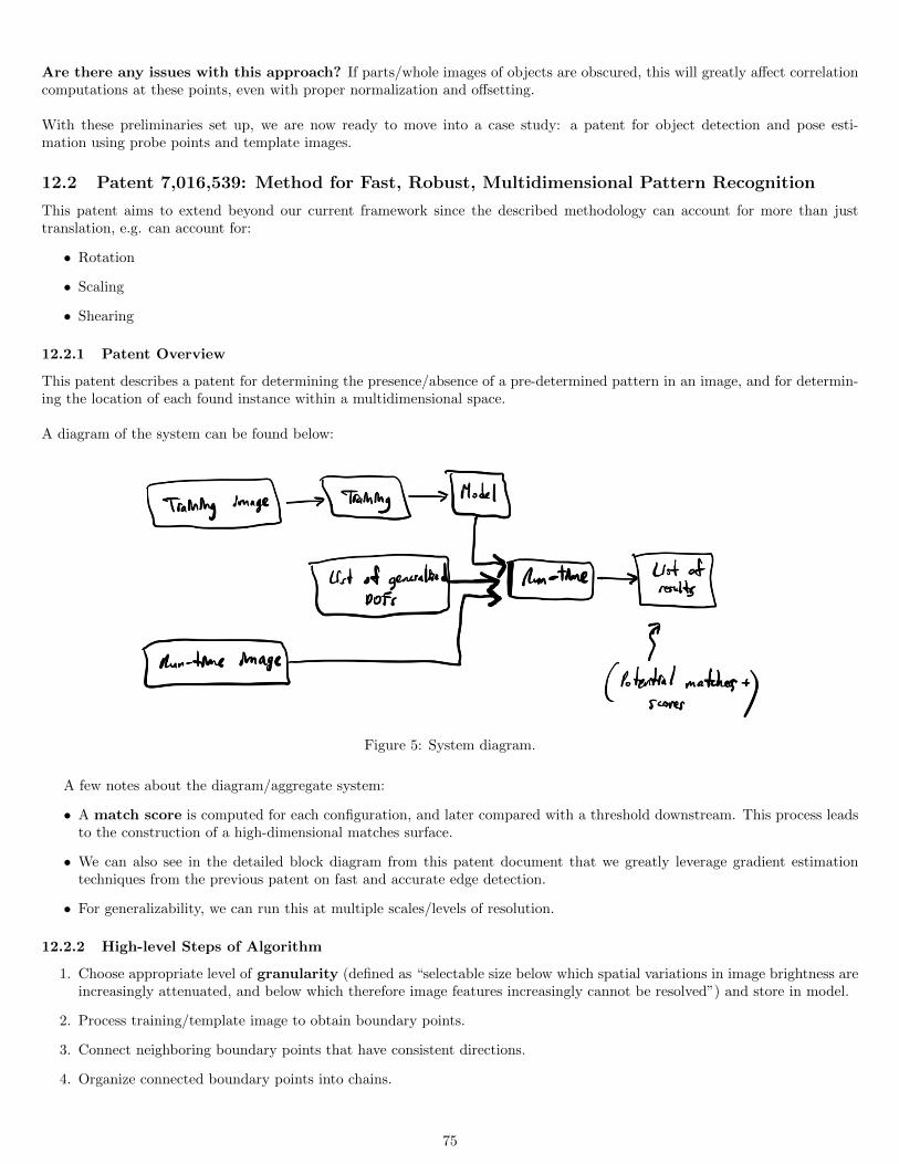
Are there any issues with this approach? If parts/whole images of objects are obscured, this will greatly affect correlationcomputations at these points, even with proper normalization and offsetting.

With these preliminaries set up, we are now ready to move into a case study: a patent for object detection and pose esti-mation using probe points and template images.

12.2 Patent 7,016,539: Method for Fast, Robust, Multidimensional Pattern Recognition

This patent aims to extend beyond our current framework since the described methodology can account for more than justtranslation, e.g. can account for:

• Rotation

• Scaling

• Shearing

12.2.1 Patent Overview

This patent describes a patent for determining the presence/absence of a pre-determined pattern in an image, and for determin-ing the location of each found instance within a multidimensional space.

A diagram of the system can be found below:

Figure 5: System diagram.

A few notes about the diagram/aggregate system:

• A match score is computed for each configuration, and later compared with a threshold downstream. This process leadsto the construction of a high-dimensional matches surface.

• We can also see in the detailed block diagram from this patent document that we greatly leverage gradient estimationtechniques from the previous patent on fast and accurate edge detection.

• For generalizability, we can run this at multiple scales/levels of resolution.

12.2.2 High-level Steps of Algorithm

1. Choose appropriate level of granularity (defined as “selectable size below which spatial variations in image brightness areincreasingly attenuated, and below which therefore image features increasingly cannot be resolved”) and store in model.

2. Process training/template image to obtain boundary points.

3. Connect neighboring boundary points that have consistent directions.

4. Organize connected boundary points into chains.

75

5. Remove short or weak chains.

6. Divide chains into segments of low curvature separated by conrner of high curvature.

7. Create evenly-spaced along segments and store them in model.

8. Determine pattern contrast and store in model.

A few notes about this procedure:

• To increase the efficiency of this approach, for storing the model, we store probes (along with granularity and contrast),not the image for which we have computed these quantities over.

• When comparing gradients between runtime and training images, project probe points onto the other image - we do nothave to look at all points in image; rather, we compare gradients (direction and magnitude - note that magnitude isoften less viable/robust to use than gradient direction) between the training and runtime images only at the probing points.

• We can also weight our probing points, either automatically or manually. Essentially, this states that some probes aremore important that others when scoring functions are called on object configurations.

• This patent can also be leveraged for machine part inspection, which necessitates high degrees of consistent accuracy

• An analog of probes in other machine and computer vision tasks is the notion of keypoints, which are used in descriptor-based feature matching algorithms such as SIFT (Scale-Invariant Feature Transform), SURF (Speeded-Up Robust Fea-tures), FAST (Features from Accelerated Segment Test), and ORB (Oriented FAST and rotated BRIEF). Many of theseaforementioned approaches rely on computing gradients at specific, “interesting points” as is done here, and constructfeatures for feature matching using a Histogram of Oriented Gradients (HoG) [1].

• For running this framework at multiple scales/resolutions, we want to use different probes at different scales.

• For multiscale, there is a need for running fast low-pass filtering. Can do so with rapid convolutions, which we will bediscussing in a later patent in this course.

• Probes “contribute evidence” individually, and are not restricted to being on the pixel grid.

• The accuracy of this approach, similar to the other framework we looked at, is limited by the degree of quantization in thesearch space.

12.2.3 Framework as Programming Objects

Let us also take a look at the object-oriented nature of this approach to better understand the framework we work with. Oneof these objects is the model:

Model: This has fields:

• Probes: This is the list of probe points. Note that we can also use compiled probes. In turn, each element in this listhas fields:

– Position

– Direction

– Weight

• Granularity: This is a scalar and is chosen during the training step.

• Contrast: This field is set to the computed contrast of the training/template pattern.

We can also look at some of the fields Generalized Degree of Freedom (Generalized DOF) object as well:

• Rotation

• Shear - The degree to which right angles are mapped into non-right angles.

• Log size

• Log x size

• Log y size

76

12.2.4 Other Considerations for this Framework

We should also consider how to run our translational search. This search should be algorithmically conducted:

• Efficiently

• At different levels of resolution

• Hexagonally, rather than on a square grid - there is a 4π advantage of work done vs. resolution. Here, hexagonal peak

detection is used, and to break ties, we arbitrarily set 3 of the 6 inequalities as ≥, and the other 3 as >.

What is pose?Pose is short for position and orientation, and is usually determined with respect to a reference coordinate system. In thepatent’s definition, it is the “mapping from pattern to image coordinates that represents a specific transformationand superposition of a pattern onto an image.”

Next, let us look into addressing “noise”, which can cause random matches to occur. Area under S(θ) curve captures theprobability of random matches, and we can compensate by calculating error and subtracting it out of the results. However, evenwith this compensation, we are still faced with additional noise in the result.

Instead, we can try to assign scoring weights by taking the dot product between gradient vectors: v1 · v2 = cos θ. But onedisadvantage of this approach is that we end up quantizing pose space.

Finally, let us look at how we score the matches between template and runtime image configurations: scoring functions.Our options are:

• Normalized correlation (above)

• Simple peak finding

• Removal of random matches (this was our “N” factor introduced above)

12.3 References

1. Histogram of Oriented Gradients, https://en.wikipedia.org/wiki/Histogram of oriented gradients

13 Lecture 14: Inspection in PatQuick, Hough Transform, Homography, Po-sition Determination, Multi-Scale

In this lecture, we will continue our discussion of “PatQuick”, the patent we discussed last time for object detection and poseestimation. We will focus on elements of this patent such as scoring functions and generalized degrees of freedom (DOF), andwill use this as a segway into general linear transformations and homography. We will conclude our discussion with subsamplingand Hough Transforms, which, at a high level, we can think of as a mapping from image space to parameter space.

13.1 Review of “PatQuick”

To frame our analysis and introduction of other technical machine vision concepts, let us briefly revisit the high-level ideas of“PatQuick”. There were three main “objects” in this model:

• Training/template image. This produces a model consisting of probe points.

• Model, containing probe points.

• Probe points, which encode evidence for where to make gradient comparisons, i.e. to determine how good matchesbetween the template image and the runtime image under the current pose configuration.

Once we have the model from the training step, we can summarize the process for generating matches as:

1. Loop over/sample from configurations of the pose space (which is determined and parameterized by our degrees of freedom),and modify the runtime image according to the current pose configuration.

2. Using the probe points of the model, compare the gradient direction (or magnitude, depending on the scoring function)to the gradient direction (magnitude) of the runtime image under the current configuration, and score using one of thescoring functions below.

77

3. Running this for all/all sampled pose configurations from the pose space produces a multidimensional scoring surface. Wecan find matches by looking for peak values in this surface.

A few more notes on this framework, before diving into the math:

• Training is beneficial here, because it allows for some degree of automated learning.

• Evidence collected from the probe points is cumulative and computed using many local operations.

• Accuracy is limited by the quantization level of the pose spanned. The non-redundant components of this pose space are:

– 2D Translation, 2 DOF

– Rotation, 1 DOF

– Scaling, 1 DOF,

– Skew, 1 DOF,

– Aspect Ratio, 1 DOF

Together, the space of all these components compose a general linear transformation, or an affine transformation:

x′ = a11x+ a12y + a13

y′ = a21x+ a22y + a23

While having all of these options leads to a high degree of generality, it also leads to a huge number of pose configurations,even for coarse quantization. This is due to the fact that the number of configurations grows exponentially with the numberof DOF.

13.1.1 Scoring Functions

Next, let us look at the scoring functions leveraged in this framework. Recall that there will also be random gradient matchesin the background texture - we can compute this “probability” as “noise” given by N:

N =1

2π

∫ 2π

0

Rdir(θ)dθ =3

32(Using signed values),

6

32(Using absolute values)

Where the first value ( 332 ) corresponds to the probability of receiving a match if we randomly select a probe point’s location,

the second value corresponds to taking reverse polarity into account, and the function Rdir corresponds to the scoring functionfor the gradient direction, and takes as input the difference between two directions as two-dimensional vectors. Below are thescoring functions considered. Please take note of the following abbreviations:

• pi denotes the two-dimensional location of the ith probe point after being projected onto the runtime image.

• di denotes the direction of the probe point in the template image.

• wi denotes the weight of the ith probe point, which is typically set manually or via some procedure.

• D(·) is a function that takes a two-dimensional point as input, and outputs the direction of the gradient at this point.

• Rdir is a scoring function that takes as input the norm of the difference between two vectors representing gradient directions,and returns a scalar.

• M(·) is a function that computes the magnitude of the gradient in the runtime image at the point given by its two-dimensional argument.

• Rmag is a scoring function that takes as input the magnitude of a gradient and returns a scalar. In this case, Rmag saturatesat a certain point, e.g. if limx→∞R(x) = K for some K ∈ R , and for some j ∈ R , R(j) = K,R(j + ε) = K ∀ ε ∈ [0,∞).

• N corresponds to the “noise” term computed above from random matches.

With these terms specified, we are now ready to introduce the scoring functions:

1. Piecewise-Linear Weighting with Direction and Normalization:

S1a(a) =

∑i max(wi, 0)Rdir(||D(a+ pi)− di||2)∑

i max(wi, 0)

Quick note: the function max(0, wi) is known as the Rectified Linear Unit (ReLU), and is written as ReLU(wi). Thisfunction comes up frequently in machine learning.

78

• Works with “compiled probes”. With these “compiled probes”, we only vary translation - we have already mappedpose according to the other DOFs above.

• Used in a “coarse step”.

2. Binary Weighting with Direction and Normalization

S1a(a) =

∑i(wi > 0)Rdir(||D(a+ pi)− di||2)∑

i(wi > 0)

Where the predicate (wi > 0) returns 1 if this is true, and 0 otherwise.

3. “Preferred Embodiment:

S(a) =

∑i(wi > 0)(Rdir(||D(a+ pi)− di||2)−N)

(1−N)∑i(wi > 0)

4. Raw Weights with Gradient Magnitude Scaling and No Normalization

S2(a) =∑i

wiM(a+ pi)Rdir(||D(a+ pi)− di||2)

Note that this scoring function is not normalized, and is used in the fine scanning step of the algorithm.

5. Raw Weights with Gradient Magnitude Scaling and Normalization

S3(a) =

∑i wiM(a+ pi)Rdir(||D(a+ pi)− di||2)∑

i wi

13.1.2 Additional System Considerations

Let us focus on a few additional system features to improve our understanding of the system as well as other principles of machinevision:

• Why do some of these approaches use normalization, but not others? Normalization is computationally-expensive,and approaches that avoid a normalization step typically do this to speed up computation.

• For all these scoring functions, the granularity parameter is determined by decreasing the resolution until the system nolonger performs well.

• We need to ensure we get the gradient direction right. So far, with just translation, this has not been something we needto worry about. But with our generalized linear transform space of poses, we may have to account for this. Specifically:

– Translation

– Rotation

– Scaling

do not affect the gradient directions. However:

– Shear

– Aspect ratio

will both affect the gradient directions. We can account for this, however, using the following process:

1. Compute the gradient in the runtime image prior to invoking any transformations on it.

2. Compute the isophote in the pre-transformed runtime image by rotating 90 degrees from the gradient direction usingthe rotation matrix given by:

RG→I =

[0 1−1 0

]3. Transform the isophote according to the generalized linear transformation above with the degrees of freedom we

consider for our pose space.

4. After computing this transformed isophote, we can find the transformed gradient by finding the direction orthogonalto the transformed isophote by rotating back 90 degrees using the rotation matrix given by:

RI→G =

[0 −11 0

]

79

13.1.3 Another Application of “PatQuick”: Machine Inspection

Let us consider some elements of this framework that make it amenable and applicable for industrial machine part inspection:

• How do we distinguish between multiple objects (a task more generally known as multiclass object detection and classifi-cation)? We can achieve this by using multiple models/template images, i.e. one model/template for each typeof object we want to detect and find the relative pose of.

• With this framework, we can also compute fractional matches - i.e. how well does one template match another object inthe runtime image.

• We can also take an edge-based similarity perspective - we can look at the runtime image’s edge and compare to edgematches achieved with the model.

13.2 Intro to Homography and Relative Poses

We will now shift gears and turn toward a topic that will also be relevant in the coming lectures on 3D. Let’s revisit ourperspective projection equations when we have a camera-centric coordinate system:

x

f=Xc

Yc,y

f=YcYc

Thus far, we have only considered camera-centric coordinate systems - that is, when the coordinates are from the point of viewof the camera. But what if we seek to image points that are in a coordinate system defined by some world coordinate systemthat differs from the camera? Then, we can express these camera coordinates as:Xc

YcZc

=

r11 r12 r13

r21 r22 r23

r31 r32 r33

XW

YWZW

+

X0

Y0

Z0

cam coord. = world2cam rot× world coord. + world2cam trans

WhereR =

r11 r12 r13

r21 r22 r23

r31 r32 r33

is a rotation matrix in 3D.

Therefore, in the general case, to find the perspective projection from world coordinates onto our image, we can combine thetwo previous equations, carrying out the matrix multiplication along the way:

x

f=Xc

Zc=r11XW + r12YW + r13ZW +X0

r31XW + r32YW + r33ZW + Z0

y

f=YcZc

=r21XW + r22YW + r23ZW + Y0

r31XW + r32YW + r33ZW + Z0

Is there a way we can combine rotation and translation into a single operation? Let us consider a simple case in which thethe points in our world coordinate system are coplanar in the three-dimensional plane ZW = 0. Since the third column of therotation corresponds to all zeros, we can rewrite our equation from the world coordinate frame to the camera frame as:Xc

YcZc

=

r11 r12 X0

r21 r22 Y0

r31 r32 Z0

XW

YW1

= T

XW

YW1

=

r11 r12 r13

r21 r22 r23

r31 r32 r33

XW

YW0

+

X0

Y0

Z0

The vector

[XW YW 1

]Texpresses our (now 2D) world coordinate system in homogeneous coordinates, which have a 1

entry appended to the final element.

In this case, we can fold translation and rotation into a single matrix! We call this matrix T, and it is called a Homog-raphy Matrix that encodes both rotation and translation. We will revisit this concept when we begin our discussion of 3Dtransformations. Note that while our rotation matrix R is orthogonal, this homography matrix T is not necessarily.

80

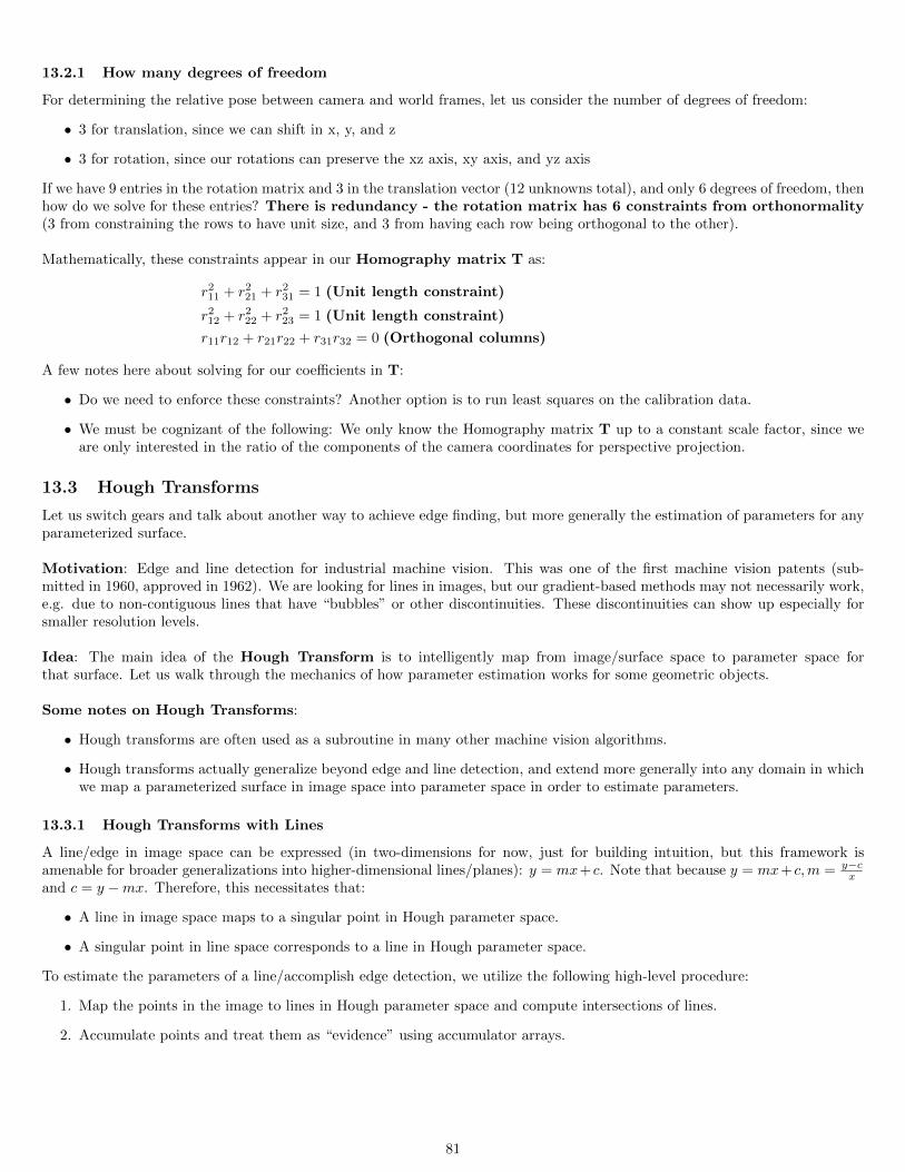
13.2.1 How many degrees of freedom

For determining the relative pose between camera and world frames, let us consider the number of degrees of freedom:

• 3 for translation, since we can shift in x, y, and z

• 3 for rotation, since our rotations can preserve the xz axis, xy axis, and yz axis

If we have 9 entries in the rotation matrix and 3 in the translation vector (12 unknowns total), and only 6 degrees of freedom, thenhow do we solve for these entries? There is redundancy - the rotation matrix has 6 constraints from orthonormality(3 from constraining the rows to have unit size, and 3 from having each row being orthogonal to the other).

Mathematically, these constraints appear in our Homography matrix T as:

r211 + r2

21 + r231 = 1 (Unit length constraint)

r212 + r2

22 + r223 = 1 (Unit length constraint)

r11r12 + r21r22 + r31r32 = 0 (Orthogonal columns)

A few notes here about solving for our coefficients in T:

• Do we need to enforce these constraints? Another option is to run least squares on the calibration data.

• We must be cognizant of the following: We only know the Homography matrix T up to a constant scale factor, since weare only interested in the ratio of the components of the camera coordinates for perspective projection.

13.3 Hough Transforms

Let us switch gears and talk about another way to achieve edge finding, but more generally the estimation of parameters for anyparameterized surface.

Motivation: Edge and line detection for industrial machine vision. This was one of the first machine vision patents (sub-mitted in 1960, approved in 1962). We are looking for lines in images, but our gradient-based methods may not necessarily work,e.g. due to non-contiguous lines that have “bubbles” or other discontinuities. These discontinuities can show up especially forsmaller resolution levels.

Idea: The main idea of the Hough Transform is to intelligently map from image/surface space to parameter space forthat surface. Let us walk through the mechanics of how parameter estimation works for some geometric objects.

Some notes on Hough Transforms:

• Hough transforms are often used as a subroutine in many other machine vision algorithms.

• Hough transforms actually generalize beyond edge and line detection, and extend more generally into any domain in whichwe map a parameterized surface in image space into parameter space in order to estimate parameters.

13.3.1 Hough Transforms with Lines

A line/edge in image space can be expressed (in two-dimensions for now, just for building intuition, but this framework isamenable for broader generalizations into higher-dimensional lines/planes): y = mx+ c. Note that because y = mx+ c,m = y−c

xand c = y −mx. Therefore, this necessitates that:

• A line in image space maps to a singular point in Hough parameter space.

• A singular point in line space corresponds to a line in Hough parameter space.

To estimate the parameters of a line/accomplish edge detection, we utilize the following high-level procedure:

1. Map the points in the image to lines in Hough parameter space and compute intersections of lines.

2. Accumulate points and treat them as “evidence” using accumulator arrays.

81

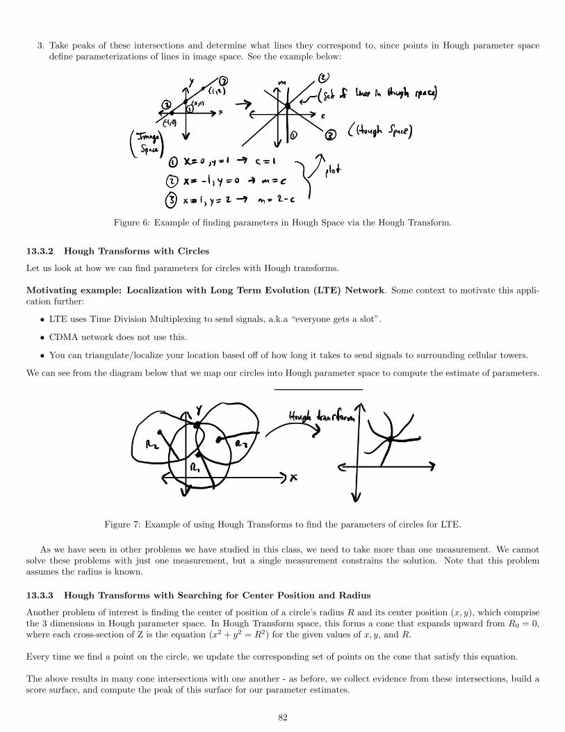
3. Take peaks of these intersections and determine what lines they correspond to, since points in Hough parameter spacedefine parameterizations of lines in image space. See the example below:

Figure 6: Example of finding parameters in Hough Space via the Hough Transform.

13.3.2 Hough Transforms with Circles

Let us look at how we can find parameters for circles with Hough transforms.

Motivating example: Localization with Long Term Evolution (LTE) Network. Some context to motivate this appli-cation further:

• LTE uses Time Division Multiplexing to send signals, a.k.a “everyone gets a slot”.

• CDMA network does not use this.

• You can triangulate/localize your location based off of how long it takes to send signals to surrounding cellular towers.

We can see from the diagram below that we map our circles into Hough parameter space to compute the estimate of parameters.

Figure 7: Example of using Hough Transforms to find the parameters of circles for LTE.

As we have seen in other problems we have studied in this class, we need to take more than one measurement. We cannotsolve these problems with just one measurement, but a single measurement constrains the solution. Note that this problemassumes the radius is known.

13.3.3 Hough Transforms with Searching for Center Position and Radius

Another problem of interest is finding the center of position of a circle’s radius R and its center position (x, y), which comprisethe 3 dimensions in Hough parameter space. In Hough Transform space, this forms a cone that expands upward from R0 = 0,where each cross-section of Z is the equation (x2 + y2 = R2) for the given values of x, y, and R.

Every time we find a point on the circle, we update the corresponding set of points on the cone that satisfy this equation.

The above results in many cone intersections with one another - as before, we collect evidence from these intersections, build ascore surface, and compute the peak of this surface for our parameter estimates.

82

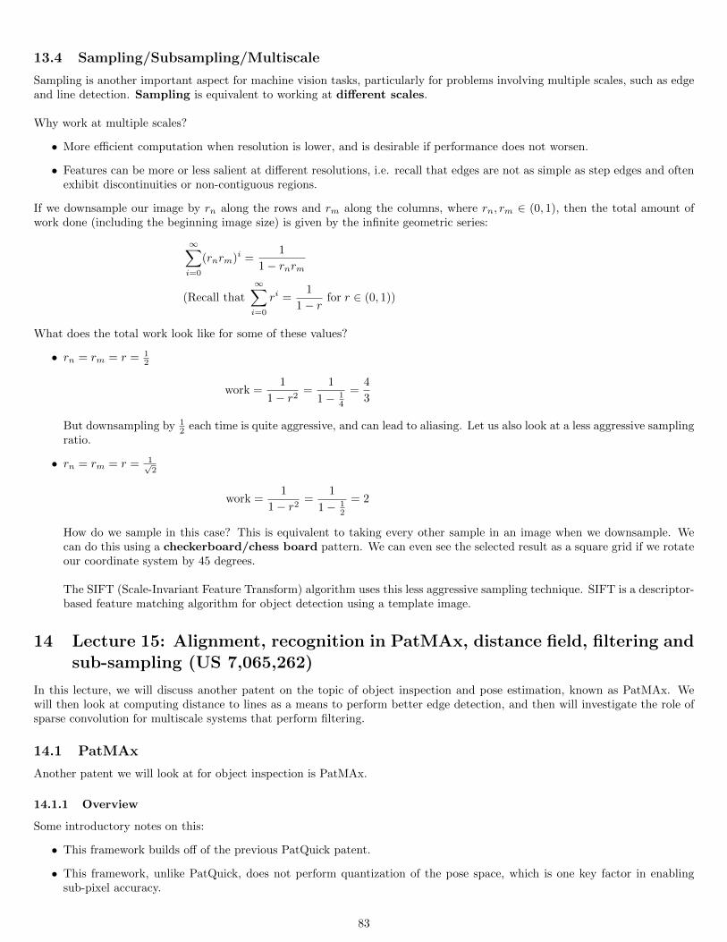
13.4 Sampling/Subsampling/Multiscale

Sampling is another important aspect for machine vision tasks, particularly for problems involving multiple scales, such as edgeand line detection. Sampling is equivalent to working at different scales.

Why work at multiple scales?

• More efficient computation when resolution is lower, and is desirable if performance does not worsen.

• Features can be more or less salient at different resolutions, i.e. recall that edges are not as simple as step edges and oftenexhibit discontinuities or non-contiguous regions.

If we downsample our image by rn along the rows and rm along the columns, where rn, rm ∈ (0, 1), then the total amount ofwork done (including the beginning image size) is given by the infinite geometric series:

∞∑i=0

(rnrm)i =1

1− rnrm

(Recall that∞∑i=0

ri =1

1− rfor r ∈ (0, 1))

What does the total work look like for some of these values?

• rn = rm = r = 12

work =1

1− r2=

1

1− 14

=4

3

But downsampling by 12 each time is quite aggressive, and can lead to aliasing. Let us also look at a less aggressive sampling

ratio.

• rn = rm = r = 1√2

work =1

1− r2=

1

1− 12

= 2

How do we sample in this case? This is equivalent to taking every other sample in an image when we downsample. Wecan do this using a checkerboard/chess board pattern. We can even see the selected result as a square grid if we rotateour coordinate system by 45 degrees.

The SIFT (Scale-Invariant Feature Transform) algorithm uses this less aggressive sampling technique. SIFT is a descriptor-based feature matching algorithm for object detection using a template image.

14 Lecture 15: Alignment, recognition in PatMAx, distance field, filtering andsub-sampling (US 7,065,262)

In this lecture, we will discuss another patent on the topic of object inspection and pose estimation, known as PatMAx. Wewill then look at computing distance to lines as a means to perform better edge detection, and then will investigate the role ofsparse convolution for multiscale systems that perform filtering.

14.1 PatMAx

Another patent we will look at for object inspection is PatMAx.

14.1.1 Overview

Some introductory notes on this:

• This framework builds off of the previous PatQuick patent.

• This framework, unlike PatQuick, does not perform quantization of the pose space, which is one key factor in enablingsub-pixel accuracy.

83

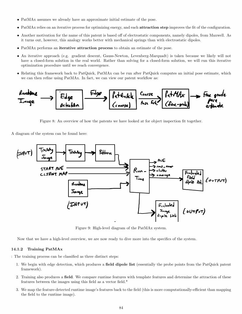
• PatMAx assumes we already have an approximate initial estimate of the pose.

• PatMAx relies on an iterative process for optimizing energy, and each attraction step improves the fit of the configuration.

• Another motivation for the name of this patent is based off of electrostatic components, namely dipoles, from Maxwell. Asit turns out, however, this analogy works better with mechanical springs than with electrostatic dipoles.

• PatMAx performs an iterative attraction process to obtain an estimate of the pose.

• An iterative approach (e.g. gradient descent, Gauss-Newton, Levenberg-Marquadt) is taken because we likely will nothave a closed-form solution in the real world. Rather than solving for a closed-form solution, we will run this iterativeoptimization procedure until we reach convergence.

• Relating this framework back to PatQuick, PatMAx can be run after PatQuick computes an initial pose estimate, whichwe can then refine using PatMAx. In fact, we can view our patent workflow as:

Figure 8: An overview of how the patents we have looked at for object inspection fit together.

A diagram of the system can be found here:

Figure 9: High-level diagram of the PatMAx system.

Now that we have a high-level overview, we are now ready to dive more into the specifics of the system.

14.1.2 Training PatMAx

: The training process can be classified as three distinct steps:

1. We begin with edge detection, which produces a field dipole list (essentially the probe points from the PatQuick patentframework).

2. Training also produces a field. We compare runtime features with template features and determine the attraction of thesefeatures between the images using this field as a vector field.*

3. We map the feature-detected runtime image’s features back to the field (this is more computationally-efficient than mappingthe field to the runtime image).

84

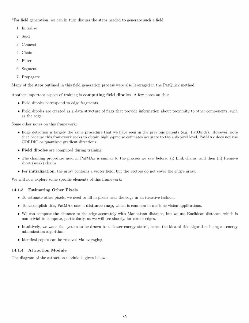
*For field generation, we can in turn discuss the steps needed to generate such a field:

1. Initialize

2. Seed

3. Connect

4. Chain

5. Filter

6. Segment

7. Propagate

Many of the steps outlined in this field generation process were also leveraged in the PatQuick method.

Another important aspect of training is computing field dipoles. A few notes on this:

• Field dipoles correspond to edge fragments.

• Field dipoles are created as a data structure of flags that provide information about proximity to other components, suchas the edge.

Some other notes on this framework:

• Edge detection is largely the same procedure that we have seen in the previous patents (e.g. PatQuick). However, notethat because this framework seeks to obtain highly-precise estimates accurate to the sub-pixel level, PatMAx does not useCORDIC or quantized gradient directions.

• Field dipoles are computed during training.

• The chaining procedure used in PatMAx is similar to the process we saw before: (i) Link chains, and then (ii) Removeshort (weak) chains.

• For initialization, the array contains a vector field, but the vectors do not cover the entire array.

We will now explore some specific elements of this framework:

14.1.3 Estimating Other Pixels

• To estimate other pixels, we need to fill in pixels near the edge in an iterative fashion.

• To accomplish this, PatMAx uses a distance map, which is common in machine vision applications.

• We can compute the distance to the edge accurately with Manhattan distance, but we use Euclidean distance, which isnon-trivial to compute, particularly, as we will see shortly, for corner edges.

• Intuitively, we want the system to be drawn to a “lower energy state”, hence the idea of this algorithm being an energyminimization algorithm.

• Identical copies can be resolved via averaging.

14.1.4 Attraction Module

The diagram of the attraction module is given below:

85

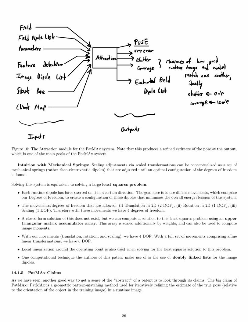
Figure 10: The Attraction module for the PatMAx system. Note that this produces a refined estimate of the pose at the output,which is one of the main goals of the PatMAx system.

Intuition with Mechanical Springs: Scaling adjustments via scaled transformations can be conceptualized as a set ofmechanical springs (rather than electrostatic dipoles) that are adjusted until an optimal configuration of the degrees of freedomis found.

Solving this system is equivalent to solving a large least squares problem:

• Each runtime dipole has force exerted on it in a certain direction. The goal here is to use diffent movements, which compriseour Degrees of Freedom, to create a configuration of these dipoles that minimizes the overall energy/tension of this system.

• The movements/degrees of freedom that are allowed: (i) Translation in 2D (2 DOF), (ii) Rotation in 2D (1 DOF), (iii)Scaling (1 DOF). Therefore with these movements we have 4 degrees of freedom.

• A closed-form solution of this does not exist, but we can compute a solution to this least squares problem using an uppertriangular matrix accumulator array. This array is scaled additionally by weights, and can also be used to computeimage moments.

• With our movements (translation, rotation, and scaling), we have 4 DOF. With a full set of movements comprising affinelinear transformations, we have 6 DOF.

• Local linearization around the operating point is also used when solving for the least squares solution to this problem.

• One computational technique the authors of this patent make use of is the use of doubly linked lists for the imagedipoles.

14.1.5 PatMAx Claims

As we have seen, another good way to get a sense of the “abstract” of a patent is to look through its claims. The big claim ofPatMAx: PatMAx is a geometric pattern-matching method used for iteratively refining the estimate of the true pose (relativeto the orientation of the object in the training image) in a runtime image.

86

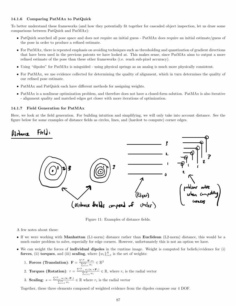
14.1.6 Comparing PatMAx to PatQuick

To better understand these frameworks (and how they potentially fit together for cascaded object inspection, let us draw somecomparisons between PatQuick and PatMAx):

• PatQuick searched all pose space and does not require an initial guess - PatMAx does require an initial estimate/guess ofthe pose in order to produce a refined estimate.

• For PatMAx, there is repeated emphasis on avoiding techniques such as thresholding and quantization of gradient directionsthat have been used in the previous patents we have looked at. This makes sense, since PatMAx aims to output a morerefined estimate of the pose than these other frameworks (i.e. reach sub-pixel accuracy).

• Using “dipoles” for PatMAx is misguided - using physical springs as an analog is much more physically consistent.

• For PatMAx, we use evidence collected for determining the quality of alignment, which in turn determines the quality ofour refined pose estimate.

• PatMAx and PatQuick each have different methods for assigning weights.

• PatMAx is a nonlinear optimization problem, and therefore does not have a closed-form solution. PatMAx is also iterative- alignment quality and matched edges get closer with more iterations of optimization.

14.1.7 Field Generation for PatMAx

Here, we look at the field generation. For building intuition and simplifying, we will only take into account distance. See thefigure below for some examples of distance fields as circles, lines, and (hardest to compute) corner edges.

Figure 11: Examples of distance fields.

A few notes about these:

• If we were working with Manhattan (L1-norm) distance rather than Euclidean (L2-norm) distance, this would be amuch easier problem to solve, especially for edge corners. However, unfortunately this is not an option we have.

• We can weight the forces of individual dipoles in the runtime image. Weight is computed for beliefs/evidence for (i)forces, (ii) torques, and (iii) scaling, where wiNi=1 is the set of weights:

1. Forces (Translation): F =∑Ni=1 Fiwi∑Ni=1 wi

∈ R2

2. Torques (Rotation): τ =∑Ni=1 wi(ri×Fi)∑N

i=1 wi∈ R, where ri is the radial vector

3. Scaling: s =∑Ni=1 wi(ri·Fi)∑N

i=1 wi∈ R where ri is the radial vector

Together, these three elements composed of weighted evidence from the dipoles compose our 4 DOF.

87

14.2 Finding Distance to Lines

One application of performing this task is to improve the performance of edge detection systems by combining shorter edgefragments of objects into longer edge fragments.

For this procedure, we break this down into two steps:

1. Rotate the 2D cartesian coordinate system into a system that is parallel to the line of interest:

x′ = x cos θ + y sin θ

y′ = −x sin θ + y cos θ

I.e.

[x′

y′

]=

[cos θ sin θ− sin θ cos θ

] [xy

]2. Translate the origin to the new location to match the line:

x′′ = x′

y′′ = y′ − ρ= −x sin θ + y cos θ − ρ

Together, these equations imply:

y′′ + x sin θ − y cos θ + ρ = 0

y′′ + x′′ sin θ − y cos θ + ρ = 0

Which in turn has the properties:

• There are no redundant solutions

• The system is parameterized by (ρ, θ)

• There are no singularities

From here, we can use the above framework to find a line by minimizing the following objective over our parameterized degreesof freedom ρ and θ:

ρ∗, θ∗ = arg minρ,θ

N∑i=1

(y′′

i )2

= arg minρ,θ

N∑i=1

(xi sin θ − yi cos θ + ρ)2

∆= arg min

ρ,θJ(ρ, θ)

This problem can be solved through our standard calculus approaches of finding the first-order conditions of our objective J(ρ, θ)on our degrees of freedom ρ and θ. Since we have two degrees of freedom, we have two First-Order Conditions:

1. ∂J(ρ,θ)∂ρ = 0:

∂

∂ρ(J(ρ, θ)) =

∂

∂ρ

( N∑i=1

(xi sin θ − yi cos θ + ρ)2)

= 2N∑i=1

(xi sin θ − yi cos θ + ρ) = 0

= sin θ( N∑i=1

xi

)− cos θ

( N∑i=1

yi

)+( N∑i=1

ρ)

= 0

= Nx sin θ −Ny cos θ +Nρ = 0

= x sin θ − y cos θ + ρ = 0

(Where x∆= 1

N

∑Ni=1 xi and y

∆= 1

N

∑Ni=1 yi.)

88

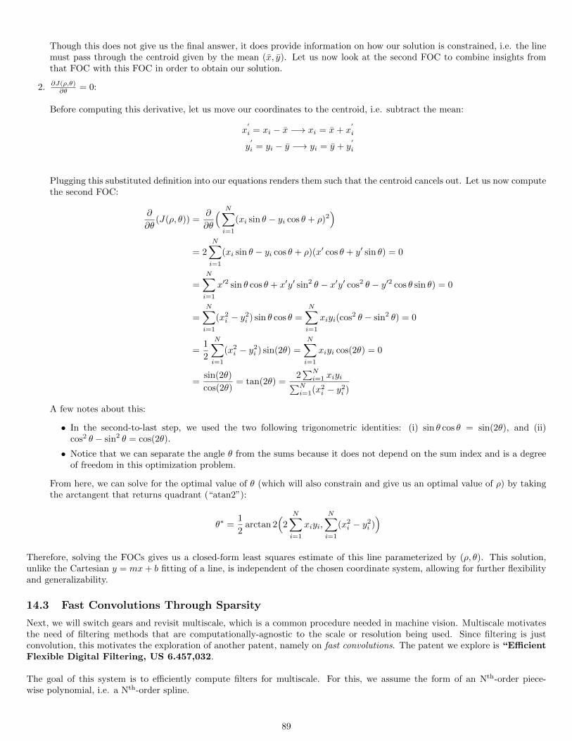
Though this does not give us the final answer, it does provide information on how our solution is constrained, i.e. the linemust pass through the centroid given by the mean (x, y). Let us now look at the second FOC to combine insights fromthat FOC with this FOC in order to obtain our solution.

2. ∂J(ρ,θ)∂θ = 0:

Before computing this derivative, let us move our coordinates to the centroid, i.e. subtract the mean:

x′

i = xi − x −→ xi = x+ x′

i

y′

i = yi − y −→ yi = y + y′

i

Plugging this substituted definition into our equations renders them such that the centroid cancels out. Let us now computethe second FOC:

∂

∂θ(J(ρ, θ)) =

∂

∂θ

( N∑i=1

(xi sin θ − yi cos θ + ρ)2)

= 2N∑i=1

(xi sin θ − yi cos θ + ρ)(x′ cos θ + y′ sin θ) = 0

=N∑i=1

x′2 sin θ cos θ + x′y′ sin2 θ − x′y′ cos2 θ − y′2 cos θ sin θ) = 0

=N∑i=1

(x2i − y2

i ) sin θ cos θ =N∑i=1

xiyi(cos2 θ − sin2 θ) = 0

=1

2

N∑i=1

(x2i − y2

i ) sin(2θ) =N∑i=1

xiyi cos(2θ) = 0

=sin(2θ)

cos(2θ)= tan(2θ) =

2∑Ni=1 xiyi∑N

i=1(x2i − y2

i )

A few notes about this:

• In the second-to-last step, we used the two following trigonometric identities: (i) sin θ cos θ = sin(2θ), and (ii)cos2 θ − sin2 θ = cos(2θ).

• Notice that we can separate the angle θ from the sums because it does not depend on the sum index and is a degreeof freedom in this optimization problem.

From here, we can solve for the optimal value of θ (which will also constrain and give us an optimal value of ρ) by takingthe arctangent that returns quadrant (“atan2”):

θ∗ =1

2arctan 2

(2N∑i=1

xiyi,N∑i=1

(x2i − y2

i ))

Therefore, solving the FOCs gives us a closed-form least squares estimate of this line parameterized by (ρ, θ). This solution,unlike the Cartesian y = mx+ b fitting of a line, is independent of the chosen coordinate system, allowing for further flexibilityand generalizability.

14.3 Fast Convolutions Through Sparsity

Next, we will switch gears and revisit multiscale, which is a common procedure needed in machine vision. Multiscale motivatesthe need of filtering methods that are computationally-agnostic to the scale or resolution being used. Since filtering is justconvolution, this motivates the exploration of another patent, namely on fast convolutions. The patent we explore is “EfficientFlexible Digital Filtering, US 6.457,032.

The goal of this system is to efficiently compute filters for multiscale. For this, we assume the form of an Nth-order piece-wise polynomial, i.e. a Nth-order spline.

89

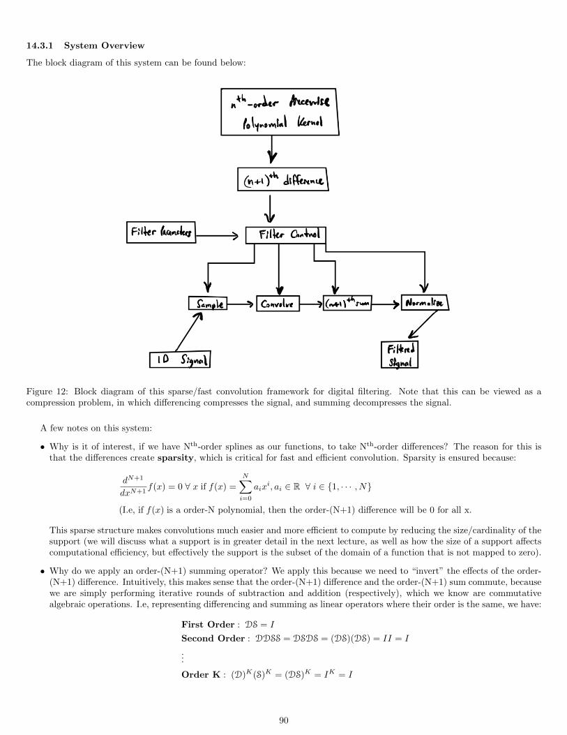
14.3.1 System Overview

The block diagram of this system can be found below:

Figure 12: Block diagram of this sparse/fast convolution framework for digital filtering. Note that this can be viewed as acompression problem, in which differencing compresses the signal, and summing decompresses the signal.

A few notes on this system:

• Why is it of interest, if we have Nth-order splines as our functions, to take Nth-order differences? The reason for this isthat the differences create sparsity, which is critical for fast and efficient convolution. Sparsity is ensured because:

dN+1

dxN+1f(x) = 0 ∀ x if f(x) =

N∑i=0

aixi, ai ∈ R ∀ i ∈ 1, · · · , N

(I.e, if f(x) is a order-N polynomial, then the order-(N+1) difference will be 0 for all x.

This sparse structure makes convolutions much easier and more efficient to compute by reducing the size/cardinality of thesupport (we will discuss what a support is in greater detail in the next lecture, as well as how the size of a support affectscomputational efficiency, but effectively the support is the subset of the domain of a function that is not mapped to zero).

• Why do we apply an order-(N+1) summing operator? We apply this because we need to “invert” the effects of the order-(N+1) difference. Intuitively, this makes sense that the order-(N+1) difference and the order-(N+1) sum commute, becausewe are simply performing iterative rounds of subtraction and addition (respectively), which we know are commutativealgebraic operations. I.e, representing differencing and summing as linear operators where their order is the same, we have:

First Order : DS = I

Second Order : DDSS = DSDS = (DS)(DS) = II = I

...

Order K : (D)K(S)K = (DS)K = IK = I

90

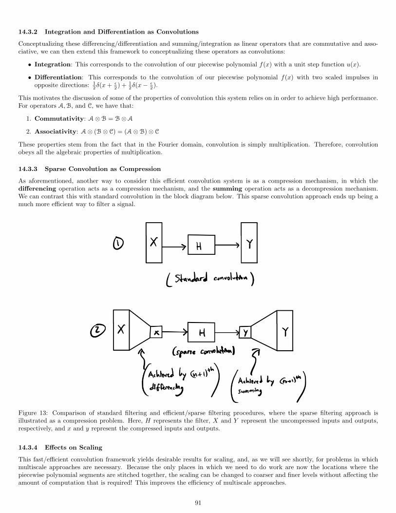
14.3.2 Integration and Differentiation as Convolutions

Conceptualizing these differencing/differentiation and summing/integration as linear operators that are commutative and asso-ciative, we can then extend this framework to conceptualizing these operators as convolutions:

• Integration: This corresponds to the convolution of our piecewise polynomial f(x) with a unit step function u(x).

• Differentiation: This corresponds to the convolution of our piecewise polynomial f(x) with two scaled impulses inopposite directions: 1

2δ(x+ ε2 ) + 1

2δ(x−ε2 ).

This motivates the discussion of some of the properties of convolution this system relies on in order to achieve high performance.For operators A,B, and C, we have that:

1. Commutativity: A⊗B = B⊗A

2. Associativity: A⊗ (B⊗ C) = (A⊗B)⊗ C

These properties stem from the fact that in the Fourier domain, convolution is simply multiplication. Therefore, convolutionobeys all the algebraic properties of multiplication.

14.3.3 Sparse Convolution as Compression

As aforementioned, another way to consider this efficient convolution system is as a compression mechanism, in which thedifferencing operation acts as a compression mechanism, and the summing operation acts as a decompression mechanism.We can contrast this with standard convolution in the block diagram below. This sparse convolution approach ends up being amuch more efficient way to filter a signal.

Figure 13: Comparison of standard filtering and efficient/sparse filtering procedures, where the sparse filtering approach isillustrated as a compression problem. Here, H represents the filter, X and Y represent the uncompressed inputs and outputs,respectively, and x and y represent the compressed inputs and outputs.

14.3.4 Effects on Scaling

This fast/efficient convolution framework yields desirable results for scaling, and, as we will see shortly, for problems in whichmultiscale approaches are necessary. Because the only places in which we need to do work are now the locations where thepiecewise polynomial segments are stitched together, the scaling can be changed to coarser and finer levels without affecting theamount of computation that is required! This improves the efficiency of multiscale approaches.

91

14.3.5 Filtering (For Multiscale): Anti-Aliasing

We have now reduced the amount of computation needed to compute efficient digital filtering. We now only need final ingredientfor multiscale that is motivated by Shannon and Nyquist: anti-aliasing methods (filters).

Recall from Shannon/Nyquist (the Sampling Theorem) that in order to sample (for instance, when we subsample in multi-scale problems) without aliasing and high-frequency artifacts, it is critical that we first remove high-frequency components fromthe signal we are sampling. This high-frequency component removal can be achieved with approximate low pass filtering (whichwe will cover in greater detail during the next lecture).

We will see in the next lecture that one way we can achieve approximate low pass filtering is by approximating a spatialsinc function (which transforms into an ideal low pass filter in the frequency domain) as a spline.

14.3.6 Extending Filtering to 2D and An Open Research Problem

This framework is built for 1D, but we note that we can extend it to 2D simply by approximating 2D convolution as a cascadedset of 1D convolutions, if we are to continue using this sparse convolution mechanism. This requires some additional run-timememory as we must store an image corresponding to the 1D convolution of the image with a 1D filter, but this allows us tocontinue using this efficient sparse convolution structure.

One open research problem: how can we extend this sparse convolution structure to 2D?

Finally, we will finish this lecture with a fun fact on calcite crystals. Calcite crystals are a type of birefringent mate-rial, which means that they have two indices of refraction that depend on two polarizations (one in the x-direction and onein the y-direction), and therefore reflect light into two different ways. As we will see in the next lecture, adding birefringentlenses in the analog domain can prevent aliasing affects from occurring that would otherwise be unavoidable. DSLRs have thesebirefringent lenses affixed to them for this specific anti-aliasing purpose.

15 Lecture 16: Fast Convolution, Low Pass Filter Approximations, IntegralImages, (US 6,457,032)

15.1 Sampling and Aliasing

Sampling is a ubiquitous operation for machine vision and general signal processing. Recall that PatMax, for instance, usessampling in its methodology. PatMax also performs an interesting operation: low-pass filtering before sampling. Why is thisperformed? To answer this question, let us revisit the Nyquist Sampling Theorem.

15.1.1 Nyquist Sampling Theorem

Before we dive into the mathematics behind this theorem, let us first build some intuition surrounding this theory.

• If we can sample a signal at a high enough frequency, we can recover the signal exactly through reconstruction.

• How is this reconstruction performed? We will convolve samples from the signal with sinc functions, and then superimposethese convolved results with one another.

• It is hard to sample from a signal with infinite support.

• What frequency do we need for this? Intuitively, to pick out how fast the signal needs to be moving, we certainly need tosample as quickly as the signal’s fastest-varying component itself. But do we need to sample even faster? It turns out theanswer is yes. As we will see below:

fmax <fsample

2=⇒ fsample > 2fmax

I.e. we will need to sample at more than twice the frequency of the highest-varying component of the signal.

Let us look at this graphically. What happens if we sample at the frequency of the signal?

92

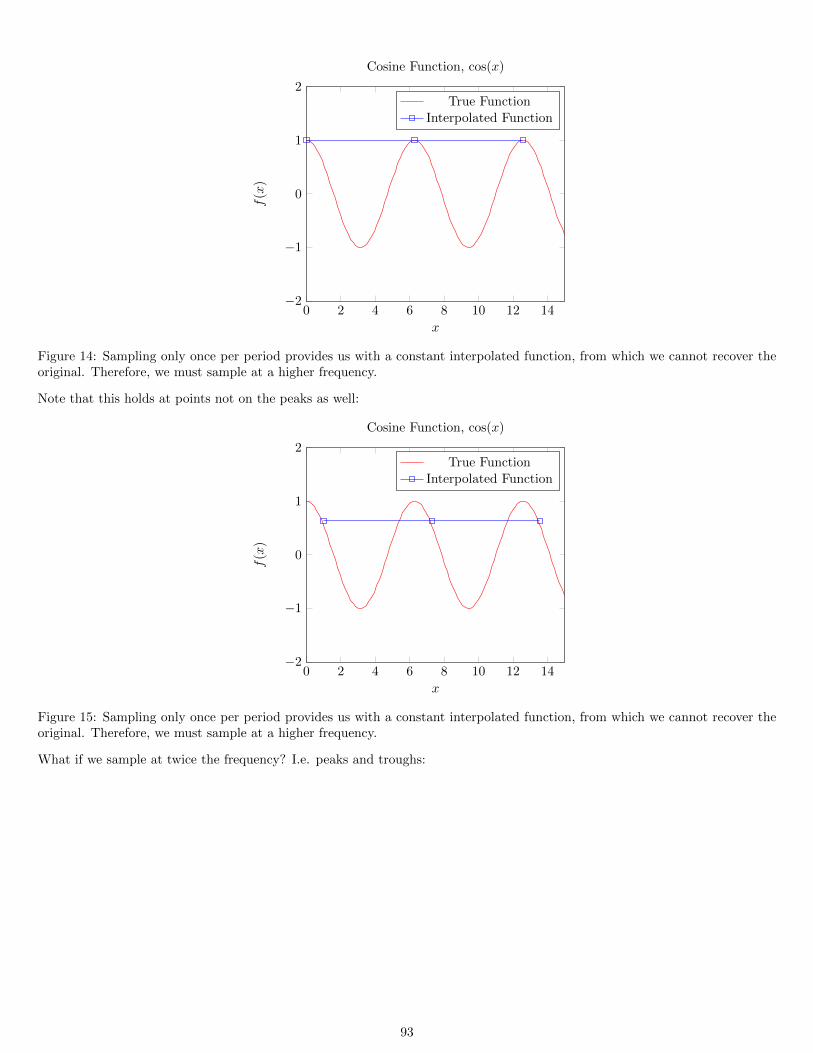
0 2 4 6 8 10 12 14−2

−1

0

1

2

x

f(x

)

Cosine Function, cos(x)

True FunctionInterpolated Function

Figure 14: Sampling only once per period provides us with a constant interpolated function, from which we cannot recover theoriginal. Therefore, we must sample at a higher frequency.

Note that this holds at points not on the peaks as well:

0 2 4 6 8 10 12 14−2

−1

0

1

2

x

f(x

)

Cosine Function, cos(x)

True FunctionInterpolated Function

Figure 15: Sampling only once per period provides us with a constant interpolated function, from which we cannot recover theoriginal. Therefore, we must sample at a higher frequency.

What if we sample at twice the frequency? I.e. peaks and troughs:

93

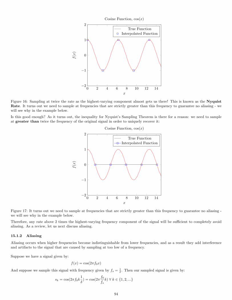
0 2 4 6 8 10 12 14−2

−1

0

1

2

x

f(x

)

Cosine Function, cos(x)

True FunctionInterpolated Function

Figure 16: Sampling at twice the rate as the highest-varying component almost gets us there! This is known as the NyquistRate. It turns out we need to sample at frequencies that are strictly greater than this frequency to guarantee no aliasing - wewill see why in the example below.

Is this good enough? As it turns out, the inequality for Nyquist’s Sampling Theorem is there for a reason: we need to sampleat greater than twice the frequency of the original signal in order to uniquely recover it:

0 2 4 6 8 10 12 14−2

−1

0

1

2

x

f(x

)

Cosine Function, cos(x)

True FunctionInterpolated Function

Figure 17: It turns out we need to sample at frequencies that are strictly greater than this frequency to guarantee no aliasing -we will see why in the example below.

Therefore, any rate above 2 times the highest-varying frequency component of the signal will be sufficient to completely avoidaliasing. As a review, let us next discuss aliasing.

15.1.2 Aliasing

Aliasing occurs when higher frequencies become indistinguishable from lower frequencies, and as a result they add interferenceand artifacts to the signal that are caused by sampling at too low of a frequency.

Suppose we have a signal given by:

f(x) = cos(2πf0x)

And suppose we sample this signal with frequency given by fs = 1δ . Then our sampled signal is given by:

sk = cos(2πf0k1

δ) = cos(2π

f0

fsk) ∀ k ∈ 1, 2, ...

94

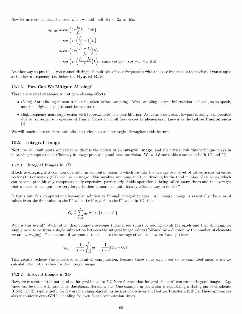
Now let us consider what happens when we add multiples of 2π to this:

sk−2π = cos(

2πf0

fsk − 2πk

)= cos

(2π(f0

fs− 1)k)

= cos(

2π(f0 − fs

fs

)k)

= cos(

2π(fs − f0

fs

)k), since cos(x) = cos(−x) ∀ x ∈ R

Another way to put this - you cannot distinguish multiples of base frequencies with the base frequencies themselves if you sampleat too low a frequency, i.e. below the Nyquist Rate.

15.1.3 How Can We Mitigate Aliasing?

There are several strategies to mitigate aliasing effects:

• (Note) Anti-aliasing measures must be taken before sampling. After sampling occurs, information is “lost”, so to speak,and the original signal cannot be recovered.

• High frequency noise suppression with (approximate) low-pass filtering. As it turns out, exact lowpass filtering is impossibledue to convergence properties of Fourier Series at cutoff frequencies (a phenomenon known as the Gibbs Phenomenon[1].

We will touch more on these anti-aliasing techniques and strategies throughout this lecture.

15.2 Integral Image

Next, we will shift gears somewhat to discuss the notion of an integral image, and the critical role this technique plays inimproving computational efficiency in image processing and machine vision. We will disucss this concept in both 1D and 2D.

15.2.1 Integral Images in 1D

Block averaging is a common operation in computer vision in which we take the average over a set of values across an entirevector (1D) or matrix (2D), such as an image. This involves summing and then dividing by the total number of elements, whichcan become prohibitively computationally-expensive, particularly if this operation is being called many times and the averagesthat we need to compute are very large. Is there a more computationally-efficient way to do this?

It turns out this computationally-simpler solution is through integral images. An integral image is essentially the sum ofvalues from the first value to the ith value, i.e if gi defines the ith value in 1D, then:

Gi∆=

i∑k=1

gk ∀ i ∈ 1, · · · ,K

Why is this useful? Well, rather than compute averages (normalized sums) by adding up all the pixels and then dividing, wesimply need to perform a single subtraction between the integral image values (followed by a division by the number of elementswe are averaging). For instance, if we wanted to calculate the average of values between i and j, then:

g[i,j] =1

j − i

j∑k=i

gk =1

j − i(Gj −Gi)

This greatly reduces the amortized amount of computation, because these sums only need to be computed once, when wecalculate the initial values for the integral image.

15.2.2 Integral Images in 2D

Now, we can extend the notion of an integral image to 2D! Note further that integral “images” can extend beyond images! E.g.these can be done with gradients, Jacobians, Hessians, etc. One example in particular is calculating a Histogram of Gradients(HoG), which is quite useful for feature matching algorithms such as Scale-Invariant Feature Transform (SIFT). These approachesalso map nicely onto GPUs, enabling for even faster computation times.

95

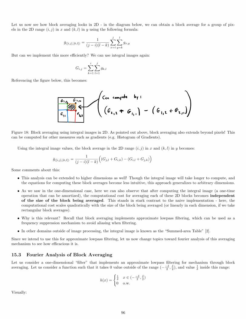
Let us now see how block averaging looks in 2D - in the diagram below, we can obtain a block average for a group of pix-els in the 2D range (i, j) in x and (k, l) in y using the following formula:

g([i,j],[k,l]) =1

(j − i)(l − k)

j∑x=i

l∑y=k

gx,y

But can we implement this more efficiently? We can use integral images again:

Gi,j =i∑

k=1

j∑l=1

gk,l

Referencing the figure below, this becomes:

Figure 18: Block averaging using integral images in 2D. As pointed out above, block averaging also extends beyond pixels! Thiscan be computed for other measures such as gradients (e.g. Histogram of Gradients).

Using the integral image values, the block average in the 2D range (i, j) in x and (k, l) in y becomes:

g([i,j],[k,l]) =1

(j − i)(l − k)

((Gj,l +Gi,k)− (Gi,l +Gj,k)

)Some comments about this:

• This analysis can be extended to higher dimensions as well! Though the integral image will take longer to compute, andthe equations for computing these block averages become less intuitive, this approach generalizes to arbitrary dimensions.

• As we saw in the one-dimensional case, here we can also observe that after computing the integral image (a one-timeoperation that can be amortized), the computational cost for averaging each of these 2D blocks becomes independentof the size of the block being averaged. This stands in stark contrast to the naive implementation - here, thecomputational cost scales quadratically with the size of the block being averaged (or linearly in each dimension, if we takerectangular block averages).

• Why is this relevant? Recall that block averaging implements approximate lowpass filtering, which can be used as afrequency suppression mechanism to avoid aliasing when filtering.

• In other domains outside of image processing, the integral image is known as the “Summed-area Table” [2].

Since we intend to use this for approximate lowpass filtering, let us now change topics toward fourier analysis of this averagingmechanism to see how efficacious it is.

15.3 Fourier Analysis of Block Averaging

Let us consider a one-dimensional “filter” that implements an approximate lowpass filtering for mechanism through blockaveraging. Let us consider a function such that it takes 0 value outside of the range (−−δ2 ,

δ2 ), and value 1

δ inside this range:

h(x) =

1δ x ∈ (−−δ2 ,

δ2 )

0 o.w.

Visually:

96

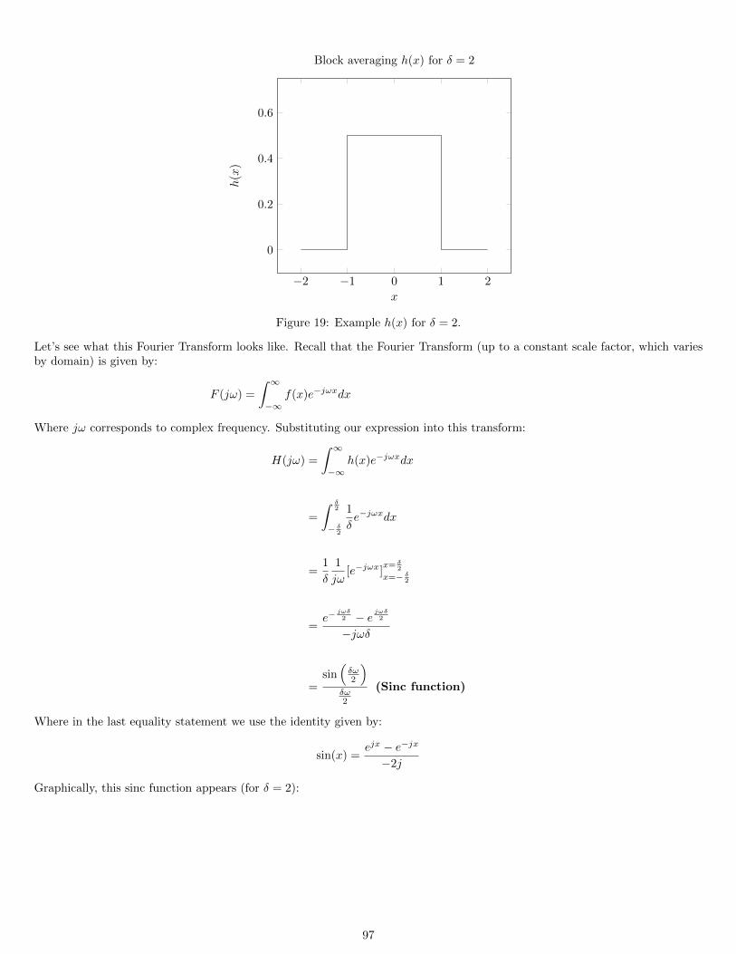
−2 −1 0 1 2

0

0.2

0.4

0.6

x

h(x

)

Block averaging h(x) for δ = 2

Figure 19: Example h(x) for δ = 2.

Let’s see what this Fourier Transform looks like. Recall that the Fourier Transform (up to a constant scale factor, which variesby domain) is given by:

F (jω) =

∫ ∞−∞

f(x)e−jωxdx

Where jω corresponds to complex frequency. Substituting our expression into this transform:

H(jω) =

∫ ∞−∞

h(x)e−jωxdx

=

∫ δ2

− δ2

1

δe−jωxdx

=1

δ

1

jω[e−jωx]

x= δ2

x=− δ2

=e−

jωδ2 − e

jωδ2

−jωδ

=sin(δω2

)δω2

(Sinc function)

Where in the last equality statement we use the identity given by:

sin(x) =ejx − e−jx

−2j

Graphically, this sinc function appears (for δ = 2):

97

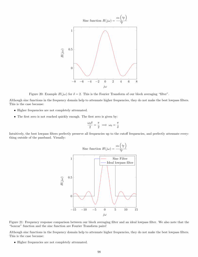
−8 −6 −4 −2 0 2 4 6 8

0

0.5

1

jω

H(jω

)

Sinc function H(jω) =sin

(δω2

)δω2

Figure 20: Example H(jω) for δ = 2. This is the Fourier Transform of our block averaging “filter”.

Although sinc functions in the frequency domain help to attenuate higher frequencies, they do not make the best lowpass filters.This is the case because:

• Higher frequencies are not completely attenuated.

• The first zero is not reached quickly enough. The first zero is given by:

ω0δ

2=π

2=⇒ ω0 =

π

δ

Intuitively, the best lowpass filters perfectly preserve all frequencies up to the cutoff frequencies, and perfectly attenuate every-thing outside of the passband. Visually:

−15 −10 −5 0 5 10 15

0

0.5

1

jω

H(jω

)

Sinc function H(jω) =sin

(δω2

)δω2

Sinc FilterIdeal lowpass filter

Figure 21: Frequency response comparison between our block averaging filter and an ideal lowpass filter. We also note that the“boxcar” function and the sinc function are Fourier Transform pairs!

Although sinc functions in the frequency domain help to attenuate higher frequencies, they do not make the best lowpass filters.This is the case because:

• Higher frequencies are not completely attenuated.

98

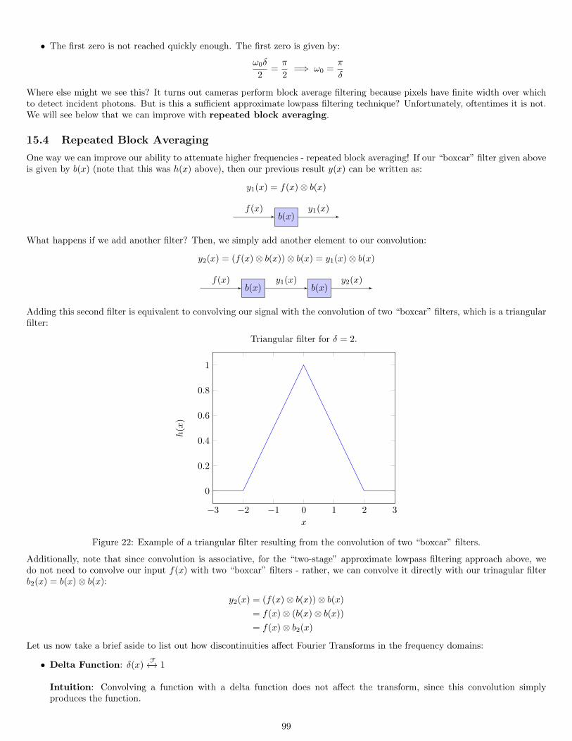
• The first zero is not reached quickly enough. The first zero is given by:

ω0δ

2=π

2=⇒ ω0 =

π

δ

Where else might we see this? It turns out cameras perform block average filtering because pixels have finite width over whichto detect incident photons. But is this a sufficient approximate lowpass filtering technique? Unfortunately, oftentimes it is not.We will see below that we can improve with repeated block averaging.

15.4 Repeated Block Averaging

One way we can improve our ability to attenuate higher frequencies - repeated block averaging! If our “boxcar” filter given aboveis given by b(x) (note that this was h(x) above), then our previous result y(x) can be written as:

y1(x) = f(x)⊗ b(x)

b(x)f(x) y1(x)

What happens if we add another filter? Then, we simply add another element to our convolution:

y2(x) = (f(x)⊗ b(x))⊗ b(x) = y1(x)⊗ b(x)

b(x) b(x)f(x) y1(x) y2(x)

Adding this second filter is equivalent to convolving our signal with the convolution of two “boxcar” filters, which is a triangularfilter:

−3 −2 −1 0 1 2 3

0

0.2

0.4

0.6

0.8

1

x

h(x

)

Triangular filter for δ = 2.

Figure 22: Example of a triangular filter resulting from the convolution of two “boxcar” filters.

Additionally, note that since convolution is associative, for the “two-stage” approximate lowpass filtering approach above, wedo not need to convolve our input f(x) with two “boxcar” filters - rather, we can convolve it directly with our trinagular filterb2(x) = b(x)⊗ b(x):

y2(x) = (f(x)⊗ b(x))⊗ b(x)

= f(x)⊗ (b(x)⊗ b(x))

= f(x)⊗ b2(x)

Let us now take a brief aside to list out how discontinuities affect Fourier Transforms in the frequency domains:

• Delta Function: δ(x)F←→ 1

Intuition: Convolving a function with a delta function does not affect the transform, since this convolution simplyproduces the function.

99

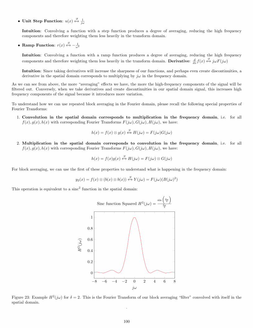
• Unit Step Function: u(x)F←→ 1

jω

Intuition: Convolving a function with a step function produces a degree of averaging, reducing the high frequencycomponents and therefore weighting them less heavily in the transform domain.

• Ramp Function: r(x)F←→ − 1

ω2

Intuition: Convolving a function with a ramp function produces a degree of averaging, reducing the high frequency

components and therefore weighting them less heavily in the transform domain. Derivative: ddxf(x)

F←→ jωF (jω)

Intuition: Since taking derivatives will increase the sharpness of our functions, and perhaps even create discontinuities, aderivative in the spatial domain corresponds to multiplying by jω in the frequency domain.

As we can see from above, the more “averaging” effects we have, the more the high-frequency components of the signal will befiltered out. Conversely, when we take derivatives and create discontinuities in our spatial domain signal, this increases highfrequency components of the signal because it introduces more variation.

To understand how we can use repeated block averaging in the Fourier domain, please recall the following special properties ofFourier Transforms:

1. Convolution in the spatial domain corresponds to multiplication in the frequency domain, i.e. for allf(x), g(x), h(x) with corresponding Fourier Transforms F (jω), G(jω), H(jω), we have:

h(x) = f(x)⊗ g(x)F←→ H(jω) = F (jω)G(jω)

2. Multiplication in the spatial domain corresponds to convolution in the frequency domain, i.e. for allf(x), g(x), h(x) with corresponding Fourier Transforms F (jω), G(jω), H(jω), we have:

h(x) = f(x)g(x)F←→ H(jω) = F (jω)⊗G(jω)

For block averaging, we can use the first of these properties to understand what is happening in the frequency domain:

y2(x) = f(x)⊗ (b(x)⊗ b(x))F←→ Y (jω) = F (jω)(B(jω)2)

This operation is equivalent to a sinc2 function in the spatial domain:

−8 −6 −4 −2 0 2 4 6 8

0

0.2

0.4

0.6

0.8

1

jω

H2(jω

)

Sinc function Squared H2(jω) =sin

(δω2

)δω2

Figure 23: Example H2(jω) for δ = 2. This is the Fourier Transform of our block averaging “filter” convolved with itself in thespatial domain.

.

100

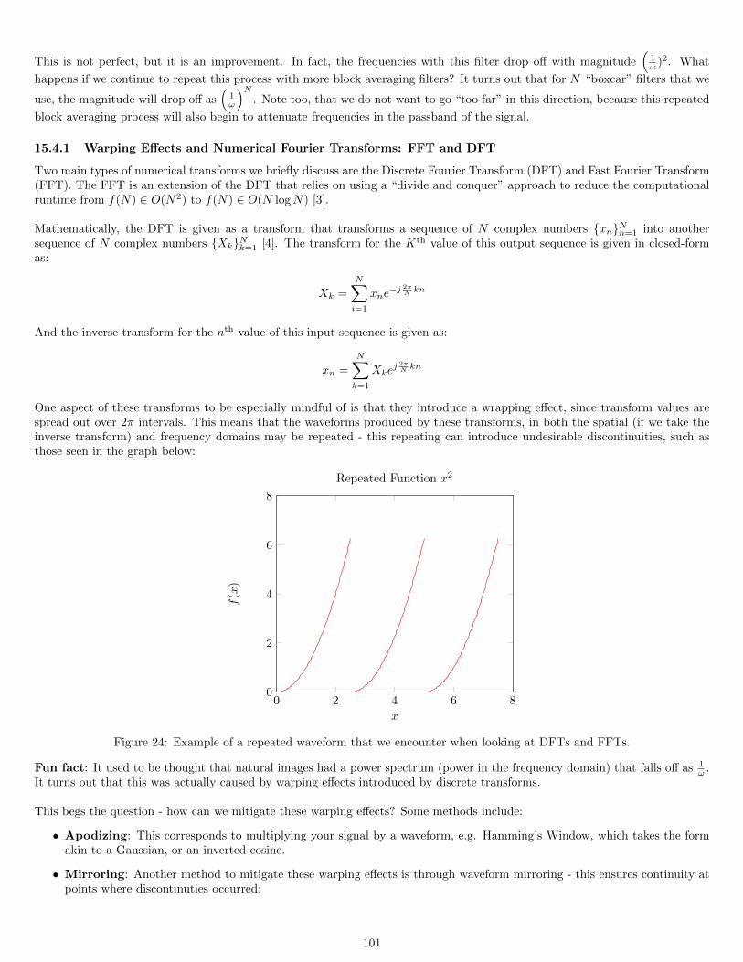
This is not perfect, but it is an improvement. In fact, the frequencies with this filter drop off with magnitude(

1ω )2. What

happens if we continue to repeat this process with more block averaging filters? It turns out that for N “boxcar” filters that we

use, the magnitude will drop off as(

1ω

)N. Note too, that we do not want to go “too far” in this direction, because this repeated

block averaging process will also begin to attenuate frequencies in the passband of the signal.

15.4.1 Warping Effects and Numerical Fourier Transforms: FFT and DFT

Two main types of numerical transforms we briefly discuss are the Discrete Fourier Transform (DFT) and Fast Fourier Transform(FFT). The FFT is an extension of the DFT that relies on using a “divide and conquer” approach to reduce the computationalruntime from f(N) ∈ O(N2) to f(N) ∈ O(N logN) [3].

Mathematically, the DFT is given as a transform that transforms a sequence of N complex numbers xnNn=1 into anothersequence of N complex numbers XkNk=1 [4]. The transform for the Kth value of this output sequence is given in closed-formas:

Xk =N∑i=1

xne−j 2π

N kn

And the inverse transform for the nth value of this input sequence is given as:

xn =N∑k=1

Xkej 2πN kn

One aspect of these transforms to be especially mindful of is that they introduce a wrapping effect, since transform values arespread out over 2π intervals. This means that the waveforms produced by these transforms, in both the spatial (if we take theinverse transform) and frequency domains may be repeated - this repeating can introduce undesirable discontinuities, such asthose seen in the graph below:

0 2 4 6 80

2

4

6

8

x

f(x

)

Repeated Function x2

Figure 24: Example of a repeated waveform that we encounter when looking at DFTs and FFTs.

Fun fact: It used to be thought that natural images had a power spectrum (power in the frequency domain) that falls off as 1ω .

It turns out that this was actually caused by warping effects introduced by discrete transforms.

This begs the question - how can we mitigate these warping effects? Some methods include:

• Apodizing: This corresponds to multiplying your signal by a waveform, e.g. Hamming’s Window, which takes the formakin to a Gaussian, or an inverted cosine.

• Mirroring: Another method to mitigate these warping effects is through waveform mirroring - this ensures continuity atpoints where discontinuties occurred:

101

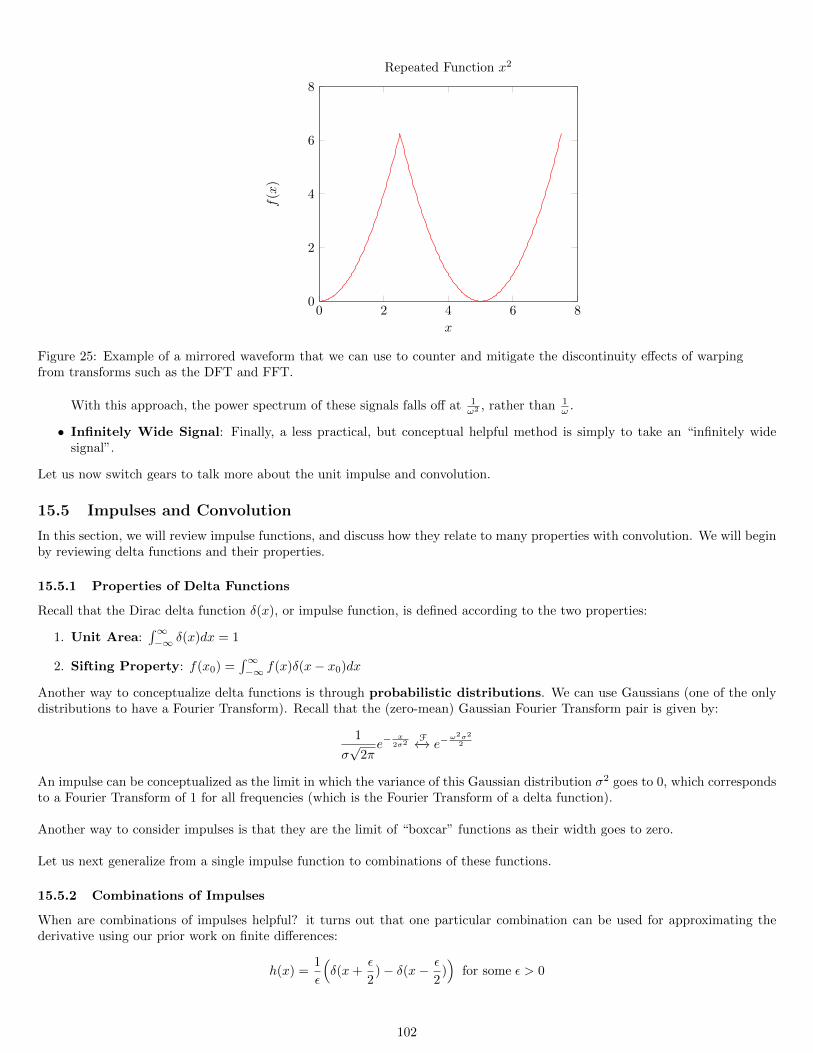
0 2 4 6 80

2

4

6

8

x

f(x

)

Repeated Function x2

Figure 25: Example of a mirrored waveform that we can use to counter and mitigate the discontinuity effects of warpingfrom transforms such as the DFT and FFT.

With this approach, the power spectrum of these signals falls off at 1ω2 , rather than 1

ω .

• Infinitely Wide Signal: Finally, a less practical, but conceptual helpful method is simply to take an “infinitely widesignal”.

Let us now switch gears to talk more about the unit impulse and convolution.

15.5 Impulses and Convolution

In this section, we will review impulse functions, and discuss how they relate to many properties with convolution. We will beginby reviewing delta functions and their properties.

15.5.1 Properties of Delta Functions

Recall that the Dirac delta function δ(x), or impulse function, is defined according to the two properties:

1. Unit Area:∫∞−∞ δ(x)dx = 1

2. Sifting Property: f(x0) =∫∞−∞ f(x)δ(x− x0)dx

Another way to conceptualize delta functions is through probabilistic distributions. We can use Gaussians (one of the onlydistributions to have a Fourier Transform). Recall that the (zero-mean) Gaussian Fourier Transform pair is given by:

1

σ√

2πe−

x2σ2

F←→ e−ω2σ2

2

An impulse can be conceptualized as the limit in which the variance of this Gaussian distribution σ2 goes to 0, which correspondsto a Fourier Transform of 1 for all frequencies (which is the Fourier Transform of a delta function).

Another way to consider impulses is that they are the limit of “boxcar” functions as their width goes to zero.

Let us next generalize from a single impulse function to combinations of these functions.

15.5.2 Combinations of Impulses

When are combinations of impulses helpful? it turns out that one particular combination can be used for approximating thederivative using our prior work on finite differences:

h(x) =1

ε

(δ(x+

ε

2)− δ(x− ε

2))

for some ε > 0

102

Correlating (*note that this is not convolution - if we were to use convolution, this derivative would be flipped) this combinationof impulse “filter” with an arbitrary function f(x), we compute a first-order approximation of the derivative:

f ′(x) ≈∫ ∞−∞

f(x)h(x)dx

=

∫ ∞−∞

(1

ε

(δ(x+

ε

2)− δ(x− ε

2)))dx

Therefore, combinations of impulses can be used to represent the same behavior as the “computational molecules” we identifiedbefore. It turns out that there is a close connection between linear, shift-invariant operators and derivative operators.

With impulses motivated, let us now formally review convolution.

15.5.3 Convolution Review

Recall from the example above that the convolution operation is simply the result of the correlation operation flipped. Mathe-matically, the convolution of functions f(x) and h(x) is given by the following commutative operation:

g(x) = f(x)⊗ h(x)

=

∫ ∞−∞

f(ξ)h(x− ξ)dξ

= h(x)⊗ g(x)

=

∫ ∞−∞

h(ξ)f(x− ξ)dξ

15.5.4 Analog Filtering with Birefringent Lenses

Why filter in the analog domain? Returning to our original problem of mitigating aliasing artifacts through high-frequencysuppression, unfortunately, if we wait to digitally filter out high frequencies after the image has already been taken by a cameraor sensor, then we have already caused aliasing.

One way to achieve this analog filtering is through Birefringent Lenses. Here, we essentially take two “shifted” imagesby convolving the image with a symmetric combination of offset delta functions, given mathematically by:

h(x) =1

2δ(x+

ε

2) +

1

2δ(x− ε

2) for some ε > 0

Let us look at the Fourier Transform of this filter, noting the following Fourier Transform pair:

δ(x− x0)F←→ e−jωx0

With this we can then express the Fourier Transform of this filter as:

F (jω) =1√2π

∫ ∞−∞

h(x)e−jωxdx

=1

2

(e−

jωε2 + e

jωε2

)= cos

(ωε2

)With this framework, the first zero to appear here occurs at ω0 = π

ε . A few notes about these filters, and how they relate tohigh-frequency noise suppression.

• When these birefringent lenses are cascaded with a block averaging filter, this results in a combined filtering scheme inwhich the zeros of the frequency responses of these filters cancel out most of the high-frequency noise.

• In the 2D case, we will have 2 birefringent filters, one for the x-direction and one for the y-direction. Physically, these arerotated 90 degrees off from one another, just as they are for a 2D cartesian coordinate system.

103

• High-performance lowpass filtering requires a large support (see definition of this below if needed) - the computationalcosts grow linearly with the size of the support in 1D, and quadratically with the size of the support in 2D. The supportof a function is defined as the set where f(·) is nonzero [5]:

supp(f) = x : f(x) 6= 0, x ∈ R

• Therefore, one way to reduce the computatonal costs of a filtering system is to reduce the size/cardinality of the support|supp(f)| - in some sense to encourage sparsity. Fortunately, this does not necessarily mean looking over a narrower range,but instead just considering less points overall.

15.5.5 Derivatives and Integrals as Convolution Operators and FT Pairs

As we have seen before, convolving a function with a unit step function results in integrating the given function. Let us verifythis below:

f(x)⊗ u(x) =

∫ ∞−∞

f(ξ)u(x− ξ)dξ

=

∫ ∞−∞

f(x− ξ)u(ξ)dξ

=

∫ ∞0

f(ξ)dξ

Therefore, we can represent integral and derivative operators as Fourier Transform pairs too, denoted S for integration and D

for derivative:

• SF←→ 1

jω

• DF←→ jω

Niote that we can verify this by showing that convolving these filter operators corresponds to multiplying these transforms infrequency space, which results in no effect when cascaded together:

(f(x)⊗D)⊗ S = f(x)⊗ (D⊗ S)F←→ F (jω)

(jω

1

jω

)= F (jω)

F←→ f(x)

S Df(x)

∫∞0f(ξ)dξ f(x)

D Sf(x) d

dxf(x) f(x)

Can we extend this to higher-order derivatives? It turns out we can. One example is the convolution of two derivative operators,which becomes:

h(x) = δ(x+ε

2)− 2δ(x) + δ(x− ε

2) = D⊗D

F←→ H(jω) = D(jω)2 = (jω)2 = −ω2 (Recall that j2 = −1)

In general, this holds. Note that the number of integral operators S must be equal to the number of derivative operators D, e.g.for K order: (

⊗Ki=1 S)⊗((⊗Ki=1 D

)⊗ f(x)

)15.5.6 Interpolation and Convolution

A few notes about interpolation methods:

• These methods work well computationally when there is sparsity in the operators we with - for instance, cubic or linearinterpolation. Photoshop and other photo-editing software frameworks iuse this interpolation techniques. Performancedeteriorates when we switch from cubic interpolation to Nearest Neighbor interpolation.

• The bicubic spline is a popular interpolation technique. It was invented by IBM and was used in early satellite imageprocessing. However, it requires many neighboring pixels, as it is composed of 7 points to interpolate over, so it is lesscomputationally-efficient.

104

• Recall that one key element of computational efficiency we pursue is to use integral images for block averaging, which ismuch more efficient than computing naive sums, especially if (1) This block averaging procedure is repeated many times(the amortized cost of computing the integral image is lessened) and (2) This process is used in higher dimensions.

• Linear interpolation can be conceptualized as connecting points together using straight lines between points. Thiscorresponds to piecewise-linear segments, or, convolution with a triangle filter, which is simply the convolution of two“boxcar filters”:

f(x) = f(1)x+ f(0)(1− x)

Unfortunately, one “not-so-great” property of convolving with triangular filters for interpolation is that the noise in theinterpolated result varies depending on how far away we are from the sampled noise.

• Nearest Neighbor techniques can also be viewed through a convolutional lens - since this method produces piecewise-constant interpolation, this is equivalent to convolving our sampled points with a “boxcar” filter!

15.5.7 Rotationally-Symmetric Lowpass Filter in 2D

Where u and v are the spatial frequencies of x and y, i.e. the 2D Fourier Transform and Inverse Fourier Transform then takethe forms of:

F (u, v) =1√2π

∫ ∞−∞

∫ ∞−∞

f(x, y)e−j(ux+vy)dxdy

f(x, y) =1√2π

∫ ∞−∞

∫ ∞−∞

F (u, v)ej(ux+vy)dudv

The inverse transform of this can be thought of as a sinc function in polar coordinates:

f(ρ, θ) =B2

2π

J1(ρB)

ρB

A few notes about this inverse transform function:

• This is the point spread function of a microscope.

• J1(·) is a 1st-order Bessel function.

• This relates to our defocusing problem that we encountered before.

• In the case of defocusing, we can use the “symmetry” property of the Fourier Transform to deduce that if we have a circularpoint spread function resulting from defocusing of the lens, then we will have a Bessel function in the frequency/Fourierdomain.

• Though a pointspread function is a “pillbox” in the ideal case, in practice this is not perfect due to artifacts such as lensaberrations.

15.6 References

1. Gibbs Phenomenon, https://en.wikipedia.org/wiki/Gibbs phenomenon

2. Summed-area Table, https://en.wikipedia.org/wiki/Summed-area table

3. Fast Fourier Transform, https://en.wikipedia.org/wiki/Fast Fourier transform

4. Discrete Fourier Transform, https://en.wikipedia.org/wiki/Discrete Fourier transform

5. Support, https://en.wikipedia.org/wiki/Support (mathematics)

16 Lecture 17: Photogrammetry, Orientation, Axes of Inertia, Symmetry, Ab-solute, Relative, Interior, and Exterior Orientation

This lecture marks a transition in what we have covered so far in the course from lower-level machine vision to higher-levelproblems, beginning with photogrammetry.

Photogrammetry: “Measurements from Imagery”, for example, map-making.

105

16.1 Photogrammetry Problems: An Overview

Four important problems in photogrammetry that we will cover are:

• Absolute Orientation 3D ←→ 3D

• Relative Orientation 2D ←→ 2D

• Exterior Orientation 2D ←→ 3D

• Intrinsic Orientation 3D ←→ 2D

Below we discuss each of these problems at a high level. We will be discussing these problems in greater depth later in this andfollowing lectures.

16.1.1 Absolute Orientation

We will start with covering absolute orientation. This problem asks about the relationship between two or more objects(cameras, points, other sensors) in 3D. Some examples of this problem include:

1. Given two 3D sensors, such as lidar (light detection and ranging) sensors, our goal is to find the transformation, or pose,between these two sensors.

2. Given one 3D sensor, such as a lidar sensor, and two objects (note that this could be two distinct objects at a single pointin time, or a single object at two distinct points in time), our goal is to find the transformation, or pose, between thetwo objects.

16.1.2 Relative Orientation

This problem asks how we can find the 2D ←→ 2D relationship between two objects, such as cameras, points, or other sensors.This type of problem comes up frequently in machine vision, for instance, binocular stereo. Two high-level applicationsinclude:

1. Given two cameras/images that these cameras take, our goal is to extract 3D information by finding the relationshipbetween two 2D images.

2. Given two cameras, our goal is to find the (relative) transformation, or pose, between the two cameras.

16.1.3 Exterior Orientation

This photogrammetry problem aims from going 2D −→ 3D. One common example in robotics (and other field related to machinevision) is localization, in which a robotic agent must find their location/orientation on a map given 2D information from acamera (as well as, possibly, 3D laser scan measurements).

More generally, with localization, our goal is to find where we are and how we are oriented in space given a 2D imageand a 3D model of the world.

16.1.4 Interior Orientation

This photogrammetry problem aims from going 3D −→ 2D. The most common application of this problem is camera calibra-tion. Camera calibration is crucial for high-precision imaging, as well as solving machine and computer vision problems such asBundle Adjustment [1]. Finding a principal point is another example of the interior orientation problem.

16.2 Absolute Orientation

We will begin our in-depth discussion and analysis of these four problems with absolute orientation. Let us start by introducingbinocular stereo.

106

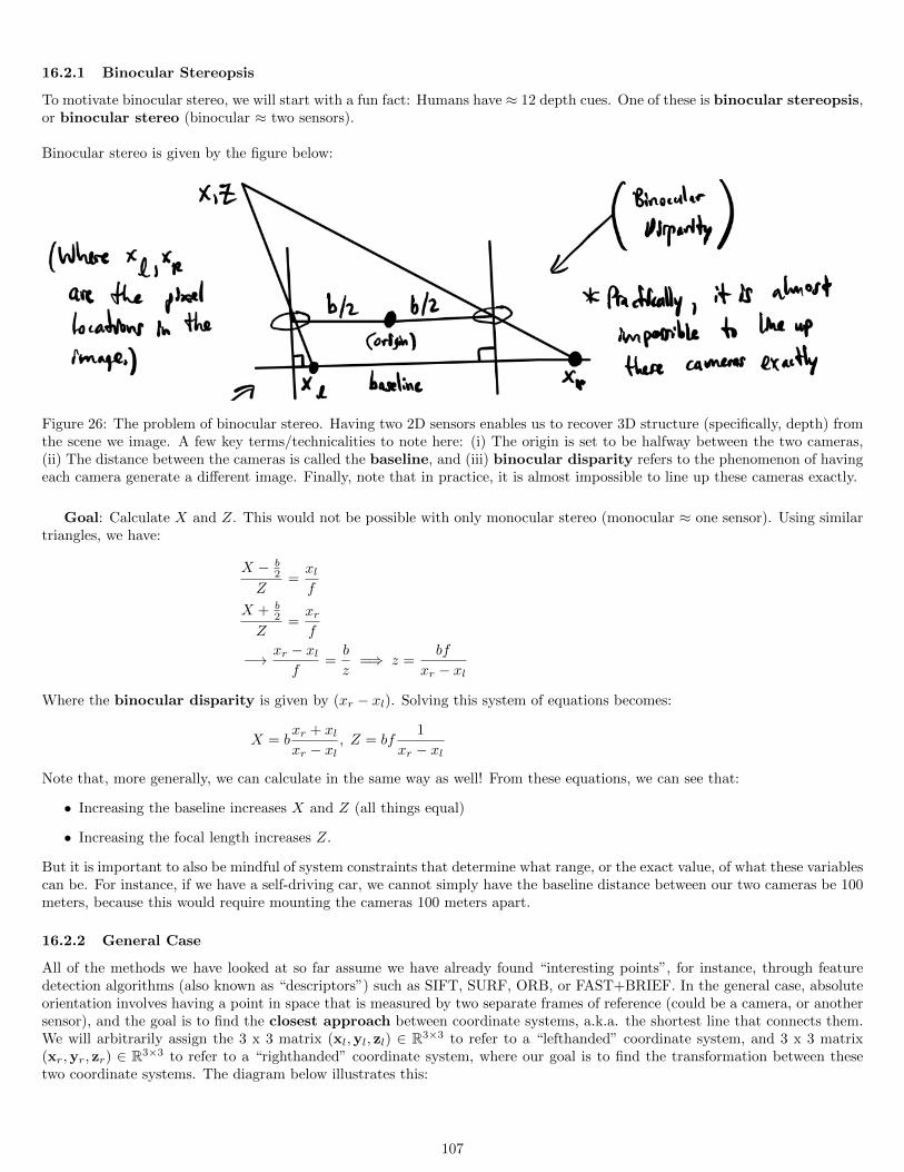
16.2.1 Binocular Stereopsis

To motivate binocular stereo, we will start with a fun fact: Humans have ≈ 12 depth cues. One of these is binocular stereopsis,or binocular stereo (binocular ≈ two sensors).

Binocular stereo is given by the figure below:

Figure 26: The problem of binocular stereo. Having two 2D sensors enables us to recover 3D structure (specifically, depth) fromthe scene we image. A few key terms/technicalities to note here: (i) The origin is set to be halfway between the two cameras,(ii) The distance between the cameras is called the baseline, and (iii) binocular disparity refers to the phenomenon of havingeach camera generate a different image. Finally, note that in practice, it is almost impossible to line up these cameras exactly.

Goal: Calculate X and Z. This would not be possible with only monocular stereo (monocular ≈ one sensor). Using similartriangles, we have:

X − b2

Z=xlf

X + b2

Z=xrf

−→ xr − xlf

=b

z=⇒ z =

bf

xr − xl

Where the binocular disparity is given by (xr − xl). Solving this system of equations becomes:

X = bxr + xlxr − xl

, Z = bf1

xr − xl

Note that, more generally, we can calculate in the same way as well! From these equations, we can see that:

• Increasing the baseline increases X and Z (all things equal)

• Increasing the focal length increases Z.

But it is important to also be mindful of system constraints that determine what range, or the exact value, of what these variablescan be. For instance, if we have a self-driving car, we cannot simply have the baseline distance between our two cameras be 100meters, because this would require mounting the cameras 100 meters apart.

16.2.2 General Case

All of the methods we have looked at so far assume we have already found “interesting points”, for instance, through featuredetection algorithms (also known as “descriptors”) such as SIFT, SURF, ORB, or FAST+BRIEF. In the general case, absoluteorientation involves having a point in space that is measured by two separate frames of reference (could be a camera, or anothersensor), and the goal is to find the closest approach between coordinate systems, a.k.a. the shortest line that connects them.We will arbitrarily assign the 3 x 3 matrix (xl,yl, zl) ∈ R3×3 to refer to a “lefthanded” coordinate system, and 3 x 3 matrix(xr,yr, zr) ∈ R3×3 to refer to a “righthanded” coordinate system, where our goal is to find the transformation between thesetwo coordinate systems. The diagram below illustrates this:

107

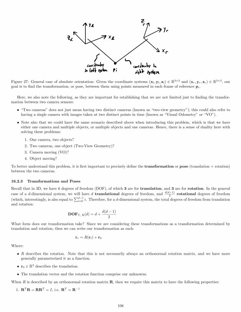
Figure 27: General case of absolute orientation: Given the coordinate systems (xl,yl, zl) ∈ R3×3 and (xr,yr, zr) ∈ R3×3, ourgoal is to find the transformation, or pose, between them using points measured in each frame of reference pi.

Here, we also note the following, as they are important for establishing that we are not limited just to finding the transfor-mation between two camera sensors:

• “Two cameras” does not just mean having two distinct cameras (known as “two-view geometry”); this could also refer tohaving a single camera with images taken at two distinct points in time (known as “Visual Odometry” or “VO”).

• Note also that we could have the same scenario described above when introducing this problem, which is that we haveeither one camera and multiple objects, or multiple objects and one cameras. Hence, there is a sense of duality here withsolving these problems:

1. One camera, two objects?

2. Two cameras, one object (Two-View Geometry)?

3. Camera moving (VO)?

4. Object moving?

To better understand this problem, it is first important to precisely define the transformation or pose (translation + rotation)between the two cameras.

16.2.3 Transformations and Poses

Recall that in 3D, we have 6 degrees of freedom (DOF), of which 3 are for translation, and 3 are for rotation. In the general

case of a d-dimensional system, we will have d translational degrees of freedom, and d(d−1)2 rotational degrees of freedom

(which, interestingly, is also equal to∑d−1i=0 i. Therefore, for a d-dimensional system, the total degrees of freedom from translation

and rotation:

DOFT, R(d) = d+d(d− 1)

2

What form does our transformation take? Since we are considering these transformations as a transformation determined bytranslation and rotation, then we can write our transformation as such:

rr = R(rl) + r0

Where:

• R describes the rotation. Note that this is not necessarily always an orthonormal rotation matrix, and we have moregenerally parameterized it as a function.

• r0 ∈ R3 describes the translation.

• The translation vector and the rotation function comprise our unknowns.

When R is described by an orthonormal rotation matrix R, then we require this matrix to have the following properties:

1. RTR = RRT = I, i.e. RT = R−1

108

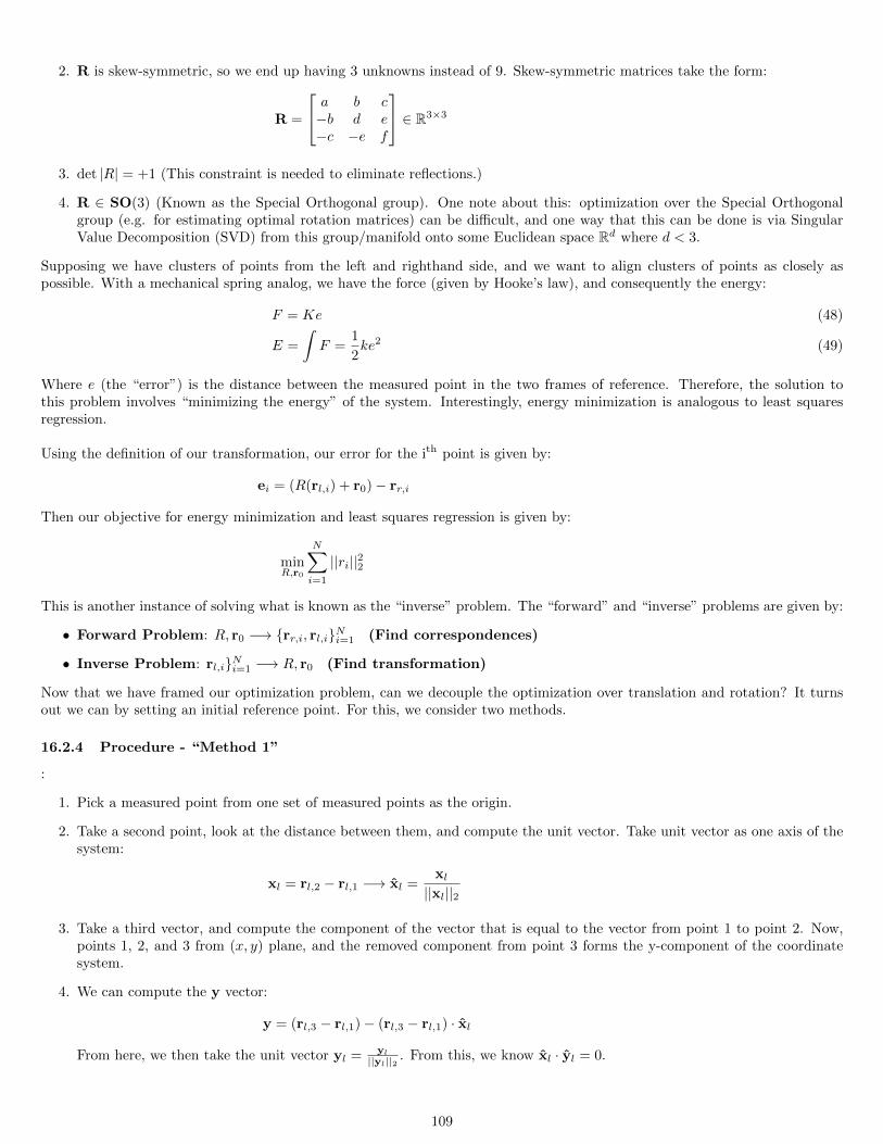
2. R is skew-symmetric, so we end up having 3 unknowns instead of 9. Skew-symmetric matrices take the form:

R =

a b c−b d e−c −e f

∈ R3×3

3. det |R| = +1 (This constraint is needed to eliminate reflections.)

4. R ∈ SO(3) (Known as the Special Orthogonal group). One note about this: optimization over the Special Orthogonalgroup (e.g. for estimating optimal rotation matrices) can be difficult, and one way that this can be done is via SingularValue Decomposition (SVD) from this group/manifold onto some Euclidean space Rd where d < 3.

Supposing we have clusters of points from the left and righthand side, and we want to align clusters of points as closely aspossible. With a mechanical spring analog, we have the force (given by Hooke’s law), and consequently the energy:

F = Ke (48)

E =

∫F =

1

2ke2 (49)

Where e (the “error”) is the distance between the measured point in the two frames of reference. Therefore, the solution tothis problem involves “minimizing the energy” of the system. Interestingly, energy minimization is analogous to least squaresregression.

Using the definition of our transformation, our error for the ith point is given by:

ei = (R(rl,i) + r0)− rr,i

Then our objective for energy minimization and least squares regression is given by:

minR,r0

N∑i=1

||ri||22

This is another instance of solving what is known as the “inverse” problem. The “forward” and “inverse” problems are given by:

• Forward Problem: R, r0 −→ rr,i, rl,iNi=1 (Find correspondences)

• Inverse Problem: rl,iNi=1 −→ R, r0 (Find transformation)

Now that we have framed our optimization problem, can we decouple the optimization over translation and rotation? It turnsout we can by setting an initial reference point. For this, we consider two methods.

16.2.4 Procedure - “Method 1”

:

1. Pick a measured point from one set of measured points as the origin.

2. Take a second point, look at the distance between them, and compute the unit vector. Take unit vector as one axis of thesystem:

xl = rl,2 − rl,1 −→ xl =xl||xl||2

3. Take a third vector, and compute the component of the vector that is equal to the vector from point 1 to point 2. Now,points 1, 2, and 3 from (x, y) plane, and the removed component from point 3 forms the y-component of the coordinatesystem.

4. We can compute the y vector:

y = (rl,3 − rl,1)− (rl,3 − rl,1) · xl

From here, we then take the unit vector yl = yl||yl||2 . From this, we know xl · yl = 0.

109

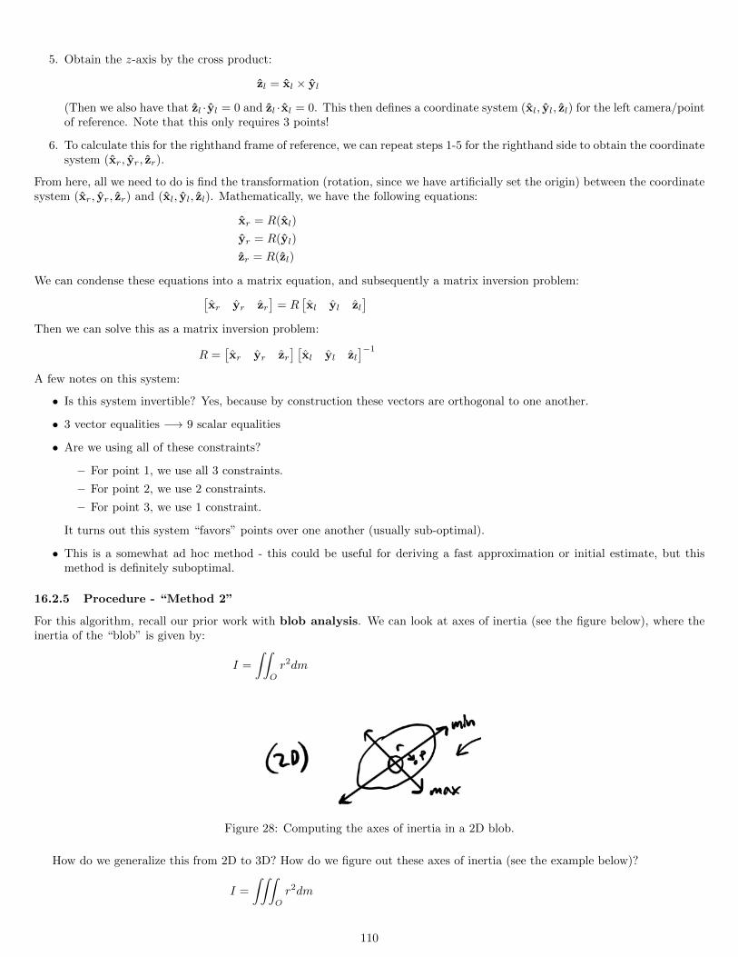
5. Obtain the z-axis by the cross product:

zl = xl × yl

(Then we also have that zl ·yl = 0 and zl ·xl = 0. This then defines a coordinate system (xl, yl, zl) for the left camera/pointof reference. Note that this only requires 3 points!

6. To calculate this for the righthand frame of reference, we can repeat steps 1-5 for the righthand side to obtain the coordinatesystem (xr, yr, zr).

From here, all we need to do is find the transformation (rotation, since we have artificially set the origin) between the coordinatesystem (xr, yr, zr) and (xl, yl, zl). Mathematically, we have the following equations:

xr = R(xl)

yr = R(yl)

zr = R(zl)

We can condense these equations into a matrix equation, and subsequently a matrix inversion problem:[xr yr zr

]= R

[xl yl zl

]Then we can solve this as a matrix inversion problem:

R =[xr yr zr

] [xl yl zl

]−1

A few notes on this system:

• Is this system invertible? Yes, because by construction these vectors are orthogonal to one another.

• 3 vector equalities −→ 9 scalar equalities

• Are we using all of these constraints?

– For point 1, we use all 3 constraints.

– For point 2, we use 2 constraints.

– For point 3, we use 1 constraint.

It turns out this system “favors” points over one another (usually sub-optimal).

• This is a somewhat ad hoc method - this could be useful for deriving a fast approximation or initial estimate, but thismethod is definitely suboptimal.

16.2.5 Procedure - “Method 2”

For this algorithm, recall our prior work with blob analysis. We can look at axes of inertia (see the figure below), where theinertia of the “blob” is given by:

I =

∫∫O

r2dm

Figure 28: Computing the axes of inertia in a 2D blob.

How do we generalize this from 2D to 3D? How do we figure out these axes of inertia (see the example below)?

I =

∫∫∫O

r2dm

110

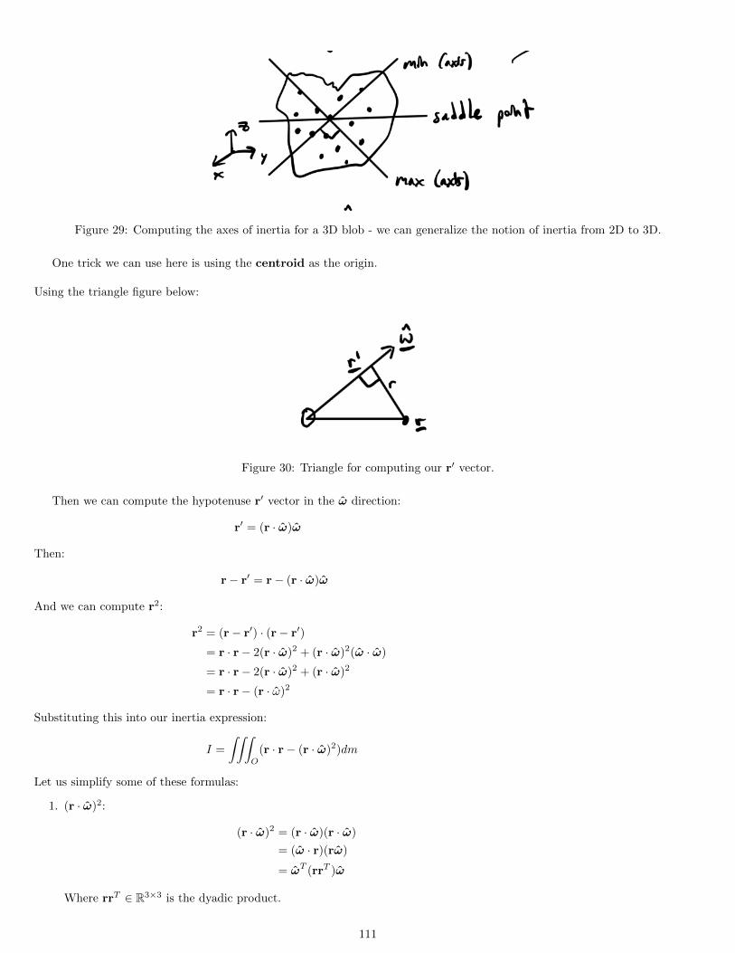
Figure 29: Computing the axes of inertia for a 3D blob - we can generalize the notion of inertia from 2D to 3D.

One trick we can use here is using the centroid as the origin.

Using the triangle figure below:

Figure 30: Triangle for computing our r′ vector.

Then we can compute the hypotenuse r′ vector in the ω direction:

r′ = (r · ω)ω

Then:

r− r′ = r− (r · ω)ω

And we can compute r2:

r2 = (r− r′) · (r− r′)

= r · r− 2(r · ω)2 + (r · ω)2(ω · ω)

= r · r− 2(r · ω)2 + (r · ω)2

= r · r− (r · ω)2

Substituting this into our inertia expression:

I =

∫∫∫O

(r · r− (r · ω)2)dm

Let us simplify some of these formulas:

1. (r · ω)2:

(r · ω)2 = (r · ω)(r · ω)

= (ω · r)(rω)

= ωT (rrT )ω

Where rrT ∈ R3×3 is the dyadic product.

111

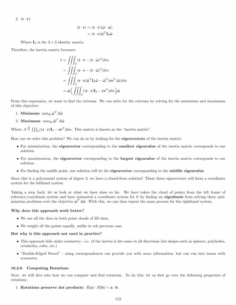
2. (r · r):

(r · r) = (r · r)(ω · ω)

= (r · r)ωT I3ω

Where I3 is the 3× 3 identity matrix.

Therefore, the inertia matrix becomes:

I =

∫∫∫O

(r · r− (r · ω)2)dm

=

∫∫∫O

(r · r− (r · ω)2)dm

=

∫∫∫O

(r · r)ωT I3ω − ωT (rrT )ω)dm

= ω(∫∫∫

O

((r · r)I3 − rrT )dm)ω

From this expression, we want to find the extrema. We can solve for the extrema by solving for the minimium and maximumsof this objective:

1. Minimum: minω ωTAω

2. Maximum: maxω ωTAω

Where A∆=∫∫∫

O((r · r)I3 − rrT )dm. This matrix is known as the “inertia matrix”.

How can we solve this problem? We can do so by looking for the eigenvectors of the inertia matrix:

• For minimization, the eigenvector corresponding to the smallest eigenvalue of the inertia matrix corresponds to oursolution.

• For maximization, the eigenvector corresponding to the largest eigenvalue of the inertia matrix corresponds to oursolution.

• For finding the saddle point, our solution will be the eigenvector corresponding to the middle eigenvalue.

Since this is a polynomial system of degree 3, we have a closed-form solution! These three eigenvectors will form a coordinatesystem for the lefthand system.

Taking a step back, let us look at what we have done so far. We have taken the cloud of points from the left frame ofreference/coordinate system and have estimated a coordinate system for it by finding an eigenbasis from solving these opti-mization problems over the objective ωTAω. With this, we can then repeat the same process for the righthand system.

Why does this approach work better?

• We use all the data in both point clouds of 3D data.

• We weight all the points equally, unlike in teh previous case.

But why is this approach not used in practice?

• This approach fails under symmetry - i.e. of the inertia is hte same in all directions (for shapes such as spheres, polyhedra,octahedra, cube, etc.)

• “Double-Edged Sword” - using correspondences can provide you with more information, but can run into issues withsymmetry.

16.2.6 Computing Rotations

Next, we will dive into how we can compute and find rotations. To do this, let us first go over the following properties ofrotations:

1. Rotations preserve dot products: R(a) ·R(b) = a · b

112

2. Rotations preserve length: R(a) ·R(a) = a · a

3. Rotations preserve angles: |R(a)×R(b)| = |a× b|

4. Rotations preserve triple products: [R(a) R(b) R(c)] = [a b c] (Where the triple product [a b c] = a · (b× c)).

Using these properties, we are now ready to set this up as least squares, using correspondences between points measured betweentwo coordinate systems:

Transform: rr = R(rl) + r0

Error: ei = rr,i −R(rl,i)− r0

And we can write our optimization as one that minimizes this error term:

R∗, r∗0

N∑i=1

||ei||2

Next, we can compute teh centroids of the left and right systems:

rl =1

N

N∑i=1

rl,i, rr =1

N

N∑i=1

rr,i

We can use these computed centroids from points so we do not have to worry about translation. A new feature of this systemis that the new centroid is at the origin. To prove this, let us “de-mean” (subtract the mean) of our coordinates in the left andrighthand coordinate systems:

r′l,i = rl,i − rl, r′r,i = rr,i − rr

Because we subtract the mean, the mean of these new points now becomes zero:

r′l =1

N

N∑i=1

r′l,i = 0 = r′r =1

N

N∑i=1

r′r,i

Substituting this back into the objective, we can solve for an optimal rotation R:

R∗ = minR,r′0

N∑i=1

||r′i −R(r′l,i − r′0)||22

= minR,r′0

N∑i=1

||r′i −R(r′l,i)||22 − 2r′0

N∑i=1

(r′r,i −R(rl,i)) +N ||r′0||22

= minR,r′0

N∑i=1

||r′i −R(r′l,i)||22 +N ||r′0||22

Since only the last term depends on r′0, we can set r′0 to minimize. Moreover, we can solve for the true r0 by back-solving later:

r0 = rr −R(rl)

Intuitively, this makes sense: the translation vector between these two coordinate systems/point clouds is the difference betweenthe centroid of the right point cloud and the centroid of the left point cloud after it has been rotated.

Since we now have that r′0 = 0 ∈ R3, we can write our error term as:

ei = r′r,i −R(r′l,i)

Which in turn allows us to write the objective as:

minN∑i=1

||ei||22 =N∑i=1

(r′r,i −R(r′l,i)(r′r,i −R(r′l,i))

=N∑i=1

||r′r,i||22 −N∑i=1

(r′r,i −R(r′l,i))−N∑i=1

||r′l,i||22

113

Where the first of these terms is fixed, the second of these terms is to be maximized (since there is a negative sign in front ofthis term, this thereby minimizes the objective), and the third of these terms is fixed. Therefore, our rotation problem can besimplified to:

minN∑i=1

||ei||22 = −2N∑i=1

(r′r,i −R(r′l,i)) (50)

To solve this objective, we could take the derivative ddR (·) of the objective, but constraints make this optimization problem

difficult to solve (note that we are not optimizing over a Euclidean search space - rather, we are optimizing over a generalizedtransformation). We will look into a different representation of R for next class to find solutions to this problem!

16.3 References

1. Bundle Adjustment, https://en.wikipedia.org/wiki/Bundle adjustment

17 Lecture 18: Rotation and How to Represent it, Unit Quaternions, theSpace of Rotations

Today, we will focus on rotations. Note that unlike translations, rotations are not commutative, which makes fittingestimates to data, amongst other machine vision tasks, more challenging. In this lecture, we will cover rotation in terms of:

• Properties

• Representations

• Hamilton’s Quaternions

• Rotation as Unit Quaternion

• Space of rotations

• Photogrammetry

• Closed-form solution of absolute quaternions

• Divison algebras, quaternion analysis, space-time

We will start by looking at some motivations for why we might care about how we formulate and formalize rotations: What isrotation used for?

• Machine vision

• Recognition/orientation

• Graphics/CAD

• Virtual Reality

• Protein Folding

• Vehicle Attitude

• Robotics

• Spatial Reasoning

• Path Planning - Collision Avoidance

114

17.1 Euclidean Motion and Rotation

Rotation and translation form Euclidean motion. Some properties of Euclidean motion, including this property. Euclideanmotion:

• Contains translation and rotation

• Preserves distances between points

• Preserves angles between lines

• Preserves handedness

• Preserves dot-products

• Preserves triple products

• Does not contain:

– Reflections

– Skewing

– Scaling

17.2 Basic Properties of Rotation

Now that we have framed rotation to be a property of Euclidean motion, we can dive further into some properties of rotation:

• Euler’s Theorem: There is a line of fixed points that remain the same in any rotation. This is known as the axis ofrotation.

• Parallel axis theorem: Any rotation is equivalent to rotation through the origin along with a translation. This allowsfor the decoupling between translation and rotation.

• Rotation of sphere includes rotation of space: I.e, any rotation that is induced on a space can be induced on anequivalent-dimensional sphere.

• Attitude, Orientation - Rotation Relative to Reference: This helps for determining the orientation of objectsrelative to another frame of reference.

• Degrees of Freedom (in 3D) is 3.

Some additional properties that are helpful for understanding rotation:

• Rotational velocity can be described by a vector. This set of rotational vectors together form a lie algebra, specifically,so(3). The set of rotations form the counterpart to this lie algebra, namely the Special Orthogonal group SO(3), whichis a Lie group. If you are not familiar with Lie groups/algebras, here are a few useful terms to get started with theseconcepts:

– A group is a set equipped with a binary operation that combines any two elements to form a third element in such away that four conditions called group axioms are satisfied, namely closure, associativity, identity and invertibility [1].

– A manifold is a d-dimensional topological space that locally resembles Euclidean space at each point i.e. any patchof the manifold can be “locally” approximated as a d-dimensional Euclidean space [2].

– A Lie group is a group that is also a differentiable manifold. One key Lie group that we will study in this course isthe Special Orthogonal group, known as SO(3), which is the space of orthonormal rotation matrices.

• We can define the derivative of the radius vector r using Poisson’s Formula: r = ω × r

• Rotational velocities add - this holds because these vectors belong to Lie algebras

• Finite rotations do not commute - this holds because rotations are defined by Lie groups in a non-Euclidean space.

• The Degrees of Freedom for rotation in dimension n is given by n(n−1)2 , which coincidentally equals 3 in 3 dimensions.

• Intuition: Oftentimes, it is easier to think about rotation “in planes”, rather than “about axes”. Rotations preservepoints in certain planes.

115

17.2.1 Isomorphism Vectors and Skew-Symmetric Matrices

A technical note that is relevant when discussing cross products: Although a cross product produces a vector in 3D, in higherdimensions the result of a cross product is a subspace, rather than a vector.

Specifically, this subspace that forms the result of a higher-dimensional cross product is the space that is perpendicu-lar/orthogonal to the two vectors the cross product operator is applied between.

With this set up, we can think of cross products as producing the following isomorphism vectors and skew-symmetric ma-trices: One Representation:

a× b = Ab

A =

0 −az ayaz 0 −ax−ay ax 0

An Isomorphic Representation:

a× b = Ba

A =

0 bz −by−bz 0 bxby −bx 0

Note that while these skew-symmetric matrices have 9 elements as they are 3× 3 matrices, they only have 3 DOF.

17.3 Representations for Rotation

There are a myriad of representations for rotations, highlighting that different applications/domains/problem-solving techniquesdemand different representations for these transformations. Some of these representations include (we will proceed in greaterdetail about these later):

1. Axis and angle

2. Euler Angles

3. Orthonormal Matrices

4. Exponential cross product

5. Stereography plus bilinear complex map

6. Pauli Spin Matrices

7. Euler Parameters

8. Unit Quaternions

Let us delve into each of these in a little more depth.

17.3.1 Axis and Angle

This representation is composed of a vector ω and an angle θ, along with the Gibb’s vector that combines these given byω tan

(θ2

), which has magnitude tan

(θ2

), providing the system with an additional degree of freedom that is not afforded by unit

vectors. Therefore, we have our full 3 rotational DOF.

17.3.2 Euler Angles

A few notes about these:

• There are over 24 definitions of Euler angles! This is the case because these definitions are permutations - i.e. the order ofthe angles matters here. The order of angular composition matters.

• These rotations are defined through each axis, roll, pitch, and yaw.

116

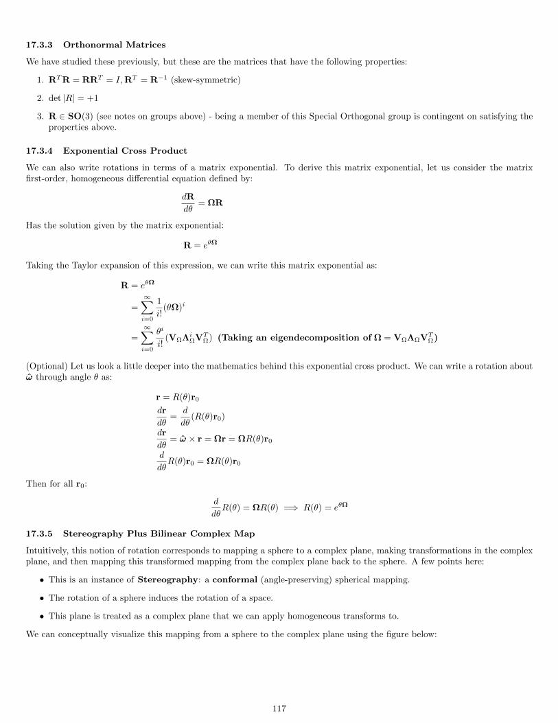
17.3.3 Orthonormal Matrices

We have studied these previously, but these are the matrices that have the following properties:

1. RTR = RRT = I,RT = R−1 (skew-symmetric)

2. det |R| = +1

3. R ∈ SO(3) (see notes on groups above) - being a member of this Special Orthogonal group is contingent on satisfying theproperties above.

17.3.4 Exponential Cross Product

We can also write rotations in terms of a matrix exponential. To derive this matrix exponential, let us consider the matrixfirst-order, homogeneous differential equation defined by:

dR

dθ= ΩR

Has the solution given by the matrix exponential:

R = eθΩ

Taking the Taylor expansion of this expression, we can write this matrix exponential as:

R = eθΩ

=∞∑i=0

1

i!(θΩ)i

=∞∑i=0

θi

i!(VΩΛi

ΩVTΩ) (Taking an eigendecomposition of Ω = VΩΛΩVT

Ω)

(Optional) Let us look a little deeper into the mathematics behind this exponential cross product. We can write a rotation aboutω through angle θ as:

r = R(θ)r0

dr

dθ=

d

dθ(R(θ)r0)

dr

dθ= ω × r = Ωr = ΩR(θ)r0

d

dθR(θ)r0 = ΩR(θ)r0

Then for all r0:

d

dθR(θ) = ΩR(θ) =⇒ R(θ) = eθΩ

17.3.5 Stereography Plus Bilinear Complex Map

Intuitively, this notion of rotation corresponds to mapping a sphere to a complex plane, making transformations in the complexplane, and then mapping this transformed mapping from the complex plane back to the sphere. A few points here:

• This is an instance of Stereography: a conformal (angle-preserving) spherical mapping.

• The rotation of a sphere induces the rotation of a space.

• This plane is treated as a complex plane that we can apply homogeneous transforms to.

We can conceptually visualize this mapping from a sphere to the complex plane using the figure below:

117

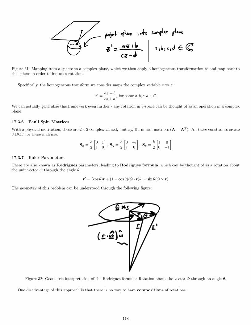
Figure 31: Mapping from a sphere to a complex plane, which we then apply a homogeneous transformation to and map back tothe sphere in order to induce a rotation.

Specifically, the homogeneous transform we consider maps the complex variable z to z′:

z′ =az + b

cz + d, for some a, b, c, d ∈ C

We can actually generalize this framework even further - any rotation in 3-space can be thought of as an operation in a complexplane.

17.3.6 Pauli Spin Matrices

With a physical motivation, these are 2× 2 complex-valued, unitary, Hermitian matrices (A = AT ). All these constraints create3 DOF for these matrices:

Sx =~2

[0 11 0

], Sy =

~2

[0 −ii 0

], Sz =

~2

[1 00 −1

]17.3.7 Euler Parameters

There are also known as Rodrigues parameters, leading to Rodrigues formula, which can be thought of as a rotation aboutthe unit vector ω through the angle θ:

r′ = (cos θ)r + (1− cos θ)(ω · r)ω + sin θ(ω × r)

The geometry of this problem can be understood through the following figure:

Figure 32: Geometric interpretation of the Rodrigues formula: Rotation about the vector ω through an angle θ.

One disadvantage of this approach is that there is no way to have compositions of rotations.

118

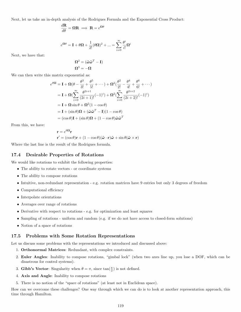
Next, let us take an in-depth analysis of the Rodrigues Formula and the Exponential Cross Product:

dR

dθ= ΩR =⇒ R = eΩθ

eΩθ = I + θΩ +1

2!(θΩ)2 + ... =

∞∑i=0

θi

i!Ωi

Next, we have that:

Ω2 = (ωωT − I)

Ω3 = −Ω

We can then write this matrix exponential as:

eθΩ = I + Ω(θ − θ3

3!+θ5

5!+ · · · ) + Ω2(

θ2

2!− θ4

4!+θ6

6!+ · · · )

= I + Ω(∞∑i=0

θ2i+1

(2i+ 1)!(−1)i) + Ω2(

∞∑i=0

θ2i+2

(2i+ 2)!(−1)i)

= I + Ω sin θ + Ω2(1− cos θ)

= I + (sin θ)Ω + (ωωT − I)(1− cos θ)

= (cos θ)I + (sin θ)Ω + (1− cos θ)ωωT

From this, we have:

r = eθΩr

r′ = (cos θ)r + (1− cos θ)(ω · r)ω + sin θ(ω × r)

Where the last line is the result of the Rodrigues formula.

17.4 Desirable Properties of Rotations

We would like rotations to exhibit the following properties:

• The ability to rotate vectors - or coordinate systems

• The ability to compose rotations

• Intuitive, non-redundant representation - e.g. rotation matrices have 9 entries but only 3 degrees of freedom

• Computational efficiency

• Interpolate orientations

• Averages over range of rotations

• Derivative with respect to rotations - e.g. for optimization and least squares

• Sampling of rotations - uniform and random (e.g. if we do not have access to closed-form solutions)

• Notion of a space of rotations

17.5 Problems with Some Rotation Representations

Let us discuss some problems with the representations we introduced and discussed above:

1. Orthonormal Matrices: Redundant, with complex constraints.

2. Euler Angles: Inability to compose rotations, “gimbal lock” (when two axes line up, you lose a DOF, which can bedisastrous for control systems).

3. Gibb’s Vector: Singularity when θ = π, since tan(π2 ) is not defined.

4. Axis and Angle: Inability to compose rotations

5. There is no notion of the “space of rotations” (at least not in Euclidean space).

How can we overcome these challenges? One way through which we can do is to look at another representation approach, thistime through Hamilton.

119

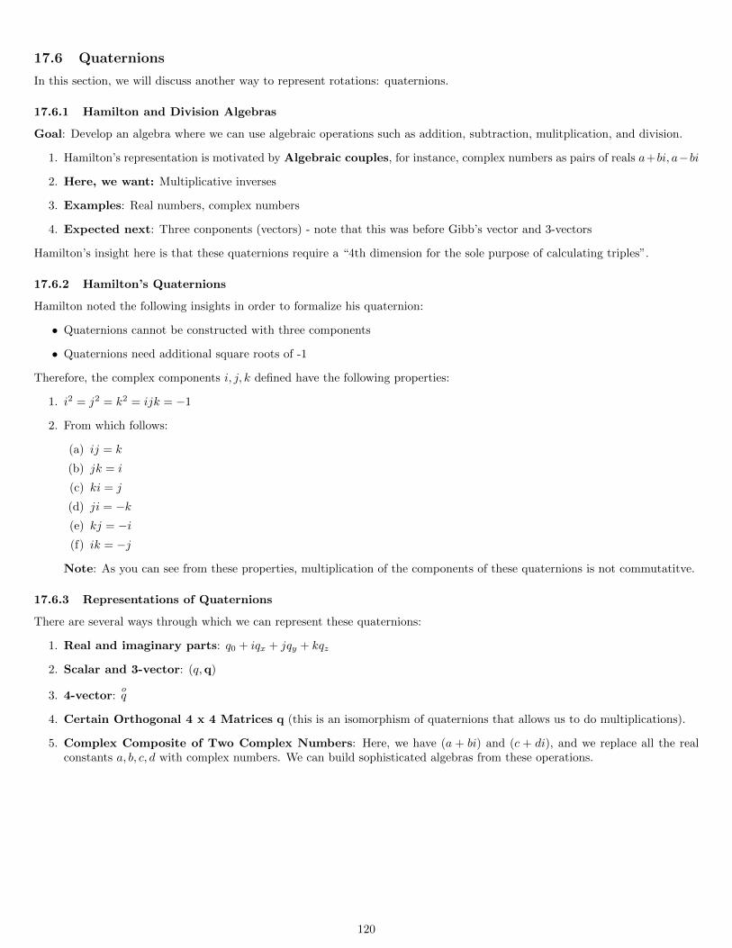
17.6 Quaternions

In this section, we will discuss another way to represent rotations: quaternions.

17.6.1 Hamilton and Division Algebras

Goal: Develop an algebra where we can use algebraic operations such as addition, subtraction, mulitplication, and division.

1. Hamilton’s representation is motivated by Algebraic couples, for instance, complex numbers as pairs of reals a+bi, a−bi

2. Here, we want: Multiplicative inverses

3. Examples: Real numbers, complex numbers

4. Expected next: Three conponents (vectors) - note that this was before Gibb’s vector and 3-vectors

Hamilton’s insight here is that these quaternions require a “4th dimension for the sole purpose of calculating triples”.

17.6.2 Hamilton’s Quaternions

Hamilton noted the following insights in order to formalize his quaternion:

• Quaternions cannot be constructed with three components

• Quaternions need additional square roots of -1

Therefore, the complex components i, j, k defined have the following properties:

1. i2 = j2 = k2 = ijk = −1

2. From which follows:

(a) ij = k

(b) jk = i

(c) ki = j

(d) ji = −k(e) kj = −i(f) ik = −j

Note: As you can see from these properties, multiplication of the components of these quaternions is not commutatitve.

17.6.3 Representations of Quaternions

There are several ways through which we can represent these quaternions:

1. Real and imaginary parts: q0 + iqx + jqy + kqz

2. Scalar and 3-vector: (q,q)

3. 4-vector:oq

4. Certain Orthogonal 4 x 4 Matrices q (this is an isomorphism of quaternions that allows us to do multiplications).

5. Complex Composite of Two Complex Numbers: Here, we have (a + bi) and (c + di), and we replace all the realconstants a, b, c, d with complex numbers. We can build sophisticated algebras from these operations.

120

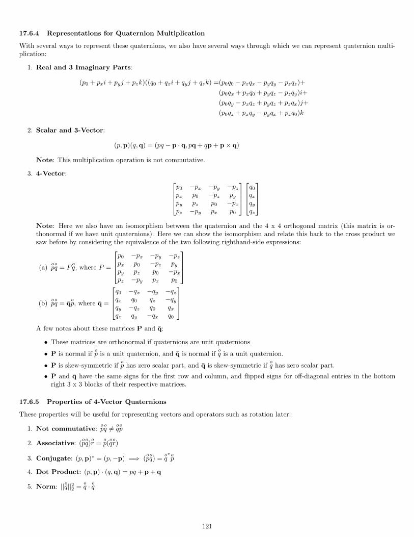
17.6.4 Representations for Quaternion Multiplication

With several ways to represent these quaternions, we also have several ways through which we can represent quaternion multi-plication:

1. Real and 3 Imaginary Parts:

(p0 + pxi+ pyj + pzk)((q0 + qxi+ qyj + qzk) =(p0q0 − pxqx − pyqy − pzqz)+(p0qx + pxq0 + pyqz − pzqy)i+

(p0qy − pxqz + pyqz + pzqx)j+

(p0qz + pxqy − pyqx + pzq0)k

2. Scalar and 3-Vector:

(p,p)(q,q) = (pq − p · q, pq + qp + p× q)

Note: This multiplication operation is not commutative.

3. 4-Vector: p0 −px −py −pzpx p0 −pz pypy pz p0 −pxpz −py px p0

q0

qxqyqz

Note: Here we also have an isomorphism between the quaternion and the 4 x 4 orthogonal matrix (this matrix is or-thonormal if we have unit quaternions). Here we can show the isomorphism and relate this back to the cross product wesaw before by considering the equivalence of the two following righthand-side expressions:

(a)opoq = P

oq, where P =

p0 −px −py −pzpx p0 −pz pypy pz p0 −pxpz −py px p0

(b)opoq = q

op, where q =

q0 −qx −qy −qzqx q0 qz −qyqy −qz q0 qxqz qy −qx q0

A few notes about these matrices P and q:

• These matrices are orthonormal if quaternions are unit quaternions

• P is normal ifop is a unit quaternion, and q is normal if

oq is a unit quaternion.

• P is skew-symmetric ifop has zero scalar part, and q is skew-symmetric if

oq has zero scalar part.

• P and q have the same signs for the first row and column, and flipped signs for off-diagonal entries in the bottomright 3 x 3 blocks of their respective matrices.

17.6.5 Properties of 4-Vector Quaternions

These properties will be useful for representing vectors and operators such as rotation later:

1. Not commutative:opoq 6= o

qop

2. Associative: (opoq)or =

op(oqor)

3. Conjugate: (p,p)∗ = (p,−p) =⇒ (opoq) =

oq∗op

4. Dot Product: (p,p) · (q,q) = pq + p + q

5. Norm: ||oq||22 =oq · oq

121

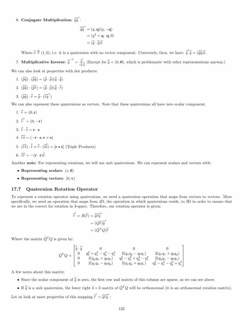
6. Conjugate Multiplication:oqoq∗:

oqoq∗

= (q,q)(q,−q)

= (q2 + q · q, 0)

= (oq · oq)oe

Whereoe

∆= (1, 0), i.e. it is a quaternion with no vector component. Conversely, then, we have:

oq∗oq = (

oqoq)oe.

7. Multiplicative Inverse:oq−1

=oq∗

(oq·oq

(Except foroq = (0,0), which is problematic with other representations anyway.)

We can also look at properties with dot products:

1. (opoq) · (opoq) = (

op · op)(oq · oq)

2. (opoq) · (opor) = (

op · op)(oq · or)

3. (opoq) · or =

op · (oroq

∗)

We can also represent these quaternions as vectors. Note that these quaternions all have zero scalar component.

1.or = (0, r)

2.or∗

= (0,−r)

3.or · os = r · s

4.oros = (−r · s, r× s)

5. (oros) ·

ot =

or · (os

ot) = [r s t] (Triple Products)

6.oror = −(r · r)

oe

Another note: For representing rotations, we will use unit quaternions. We can represent scalars and vectors with:

• Representing scalars: (s,0)

• Representing vectors: (0,v)

17.7 Quaternion Rotation Operator

To represent a rotation operator using quaternions, we need a quaternion operation that maps from vectors to vectors. Morespecifically, we need an operation that maps from 4D, the operation in which quaternions reside, to 3D in order to ensure thatwe are in the correct for rotation in 3-space. Therefore, our rotation operator is given:

or′

= R(or) =

oqoroq∗

= (Qor)oq∗

= (QTQ)or

Where the matrix QTQ is given by:

QTQ =

oq · oq 0 0 0

0 q20 + q2

x − q2y − q2

z 2(qxqy − q0qz) 2(qxqz + q0qy)0 2(qyqx + q0qz) q2

0 − q2x + q2

y − q2z 2(qyqz − q0qx)

0 2(qzqx − q0qy) 2(qzqy + q0qz) q20 − q2

x − q2y + q2

z

A few notes about this matrix:

• Since the scalar component ofoq is zero, the first row and matrix of this column are sparse, as we can see above.

• Ifoq is a unit quaternion, the lower right 3× 3 matrix of QTQ will be orthonormal (it is an orthonormal rotation matrix).

Let us look at more properties of this mappingor′

=oqoroq∗:

122

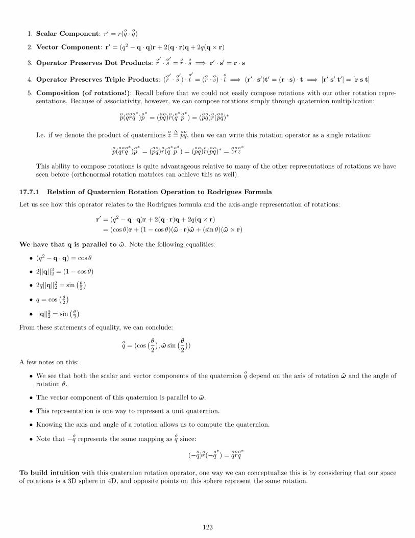
1. Scalar Component: r′ = r(oq · oq)

2. Vector Component: r′ = (q2 − q · q)r + 2(q · r)q + 2q(q× r)

3. Operator Preserves Dot Products:or′· os′

=or · os =⇒ r′ · s′ = r · s

4. Operator Preserves Triple Products: (or′· os′) ·

ot′

= (or · os) ·

ot =⇒ (r′ · s′)t′ = (r · s) · t =⇒ [r′ s′ t′] = [r s t]

5. Composition (of rotations!): Recall before that we could not easily compose rotations with our other rotation repre-sentations. Because of associativity, however, we can compose rotations simply through quaternion multiplication:

op(oqoroq∗)op∗

= (opoq)or(oq∗op∗) = (

opoq)or(opoq)∗

I.e. if we denote the product of quaternionsoz

∆=

opoq, then we can write this rotation operator as a single rotation:

op(oqoroq∗)op∗

= (opoq)or(oq∗op∗) = (

opoq)or(opoq)∗ =

ozoroz∗

This ability to compose rotations is quite advantageous relative to many of the other representations of rotations we haveseen before (orthonormal rotation matrices can achieve this as well).

17.7.1 Relation of Quaternion Rotation Operation to Rodrigues Formula

Let us see how this operator relates to the Rodrigues formula and the axis-angle representation of rotations:

r′ = (q2 − q · q)r + 2(q · r)q + 2q(q× r)

= (cos θ)r + (1− cos θ)(ω · r)ω + (sin θ)(ω × r)

We have that q is parallel to ω. Note the following equalities:

• (q2 − q · q) = cos θ

• 2||q||22 = (1− cos θ)

• 2q||q||22 = sin(θ2

)• q = cos

(θ2

)• ||q||22 = sin

(θ2

)From these statements of equality, we can conclude:

oq = (cos

(θ2

), ω sin

(θ2

))

A few notes on this:

• We see that both the scalar and vector components of the quaternionoq depend on the axis of rotation ω and the angle of

rotation θ.

• The vector component of this quaternion is parallel to ω.

• This representation is one way to represent a unit quaternion.

• Knowing the axis and angle of a rotation allows us to compute the quaternion.

• Note that −oq represents the same mapping asoq since:

(−oq)or(−oq∗) =

oqoroq∗

To build intuition with this quaternion rotation operator, one way we can conceptualize this is by considering that our spaceof rotations is a 3D sphere in 4D, and opposite points on this sphere represent the same rotation.

123

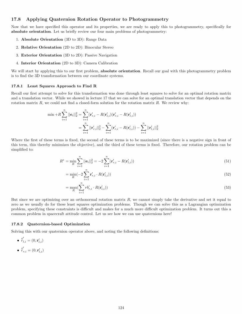
17.8 Applying Quaternion Rotation Operator to Photogrammetry

Now that we have specified this operator and its properties, we are ready to apply this to photogrammetry, specifically forabsolute orientation. Let us briefly review our four main problems of photogrammetry:

1. Absolute Orientation (3D to 3D): Range Data

2. Relative Orientation (2D to 2D): Binocular Stereo

3. Exterior Orientation (3D to 2D): Passive Navigation

4. Interior Orientation (2D to 3D): Camera Calibration

We will start by applying this to our first problem, absolute orientation. Recall our goal with this photogrammetry problemis to find the 3D transformation between our coordinate systems.

17.8.1 Least Squares Approach to Find R

Recall our first attempt to solve for this transformation was done through least squares to solve for an optimal rotation matrixand a translation vector. While we showed in lecture 17 that we can solve for an optimal translation vector that depends on therotation matrix R, we could not find a closed-form solution for the rotation matrix R. We review why:

min +Rn∑i=1

||ei||22 =n∑i=1

(r′r,i −R(r′l,i)(r′r,i −R(r′l,i))

=n∑i=1

||r′r,i||22 −n∑i=1

(r′r,i −R(r′l,i))−n∑i=1

||r′l,i||22

Where the first of these terms is fixed, the second of these terms is to be maximized (since there is a negative sign in front ofthis term, this thereby minimizes the objective), and the third of these terms is fixed. Therefore, our rotation problem can besimplified to:

R∗ = minR

n∑i=1

||ei||22 = −2

n∑i=1

(r′r,i −R(r′l,i)) (51)

= minR

(−2n∑i=1

r′r,i ·R(r′l,i)) (52)

= maxR

(n∑i=1

rb′r,i ·R(r′l,i)) (53)

But since we are optimizing over an orthonormal rotation matrix R, we cannot simply take the derivative and set it equal tozero as we usually do for these least squares optimization problems. Though we can solve this as a Lagrangian optimizationproblem, specifying these constraints is difficult and makes for a much more difficult optimization problem. It turns out this acommon problem in spacecraft attitude control. Let us see how we can use quaternions here!

17.8.2 Quaternion-based Optimization

Solving this with our quaternion operator above, and noting the following definitions:

• or′l,i = (0, r′l,i)

• or′r,i = (0, r′l,i)

124

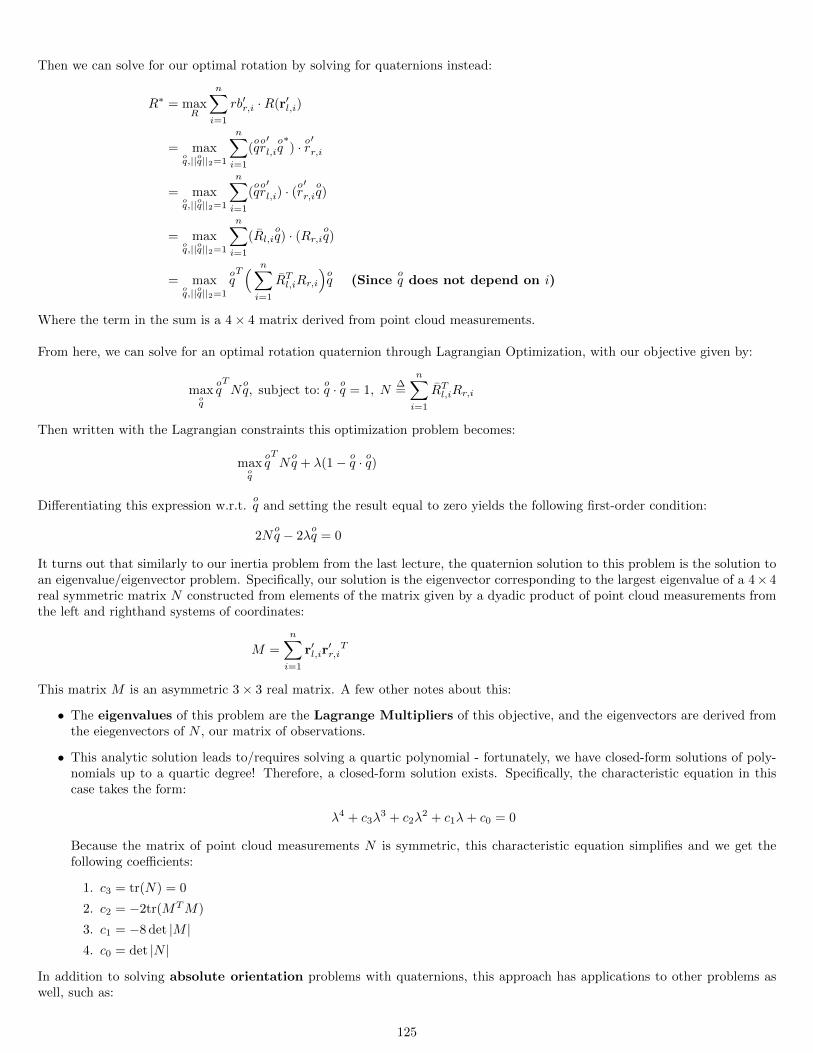
Then we can solve for our optimal rotation by solving for quaternions instead:

R∗ = maxR

n∑i=1

rb′r,i ·R(r′l,i)

= maxoq,||oq||2=1

n∑i=1

(oqor′l,i

oq∗) · or′r,i

= maxoq,||oq||2=1

n∑i=1

(oqor′l,i) · (

or′r,i

oq)

= maxoq,||oq||2=1

n∑i=1

(Rl,ioq) · (Rr,i

oq)

= maxoq,||oq||2=1

oqT( n∑

i=1

RTl,iRr,i

)oq (Since

oq does not depend on i)

Where the term in the sum is a 4× 4 matrix derived from point cloud measurements.

From here, we can solve for an optimal rotation quaternion through Lagrangian Optimization, with our objective given by:

maxoq

oqTNoq, subject to:

oq · oq = 1, N

∆=

n∑i=1

RTl,iRr,i

Then written with the Lagrangian constraints this optimization problem becomes:

maxoq

oqTNoq + λ(1− o

q · oq)

Differentiating this expression w.r.t.oq and setting the result equal to zero yields the following first-order condition:

2Noq − 2λ

oq = 0

It turns out that similarly to our inertia problem from the last lecture, the quaternion solution to this problem is the solution toan eigenvalue/eigenvector problem. Specifically, our solution is the eigenvector corresponding to the largest eigenvalue of a 4× 4real symmetric matrix N constructed from elements of the matrix given by a dyadic product of point cloud measurements fromthe left and righthand systems of coordinates:

M =n∑i=1

r′l,ir′r,iT

This matrix M is an asymmetric 3× 3 real matrix. A few other notes about this:

• The eigenvalues of this problem are the Lagrange Multipliers of this objective, and the eigenvectors are derived fromthe eiegenvectors of N , our matrix of observations.

• This analytic solution leads to/requires solving a quartic polynomial - fortunately, we have closed-form solutions of poly-nomials up to a quartic degree! Therefore, a closed-form solution exists. Specifically, the characteristic equation in thiscase takes the form:

λ4 + c3λ3 + c2λ

2 + c1λ+ c0 = 0

Because the matrix of point cloud measurements N is symmetric, this characteristic equation simplifies and we get thefollowing coefficients:

1. c3 = tr(N) = 0

2. c2 = −2tr(MTM)

3. c1 = −8 det |M |4. c0 = det |N |

In addition to solving absolute orientation problems with quaternions, this approach has applications to other problems aswell, such as:

125

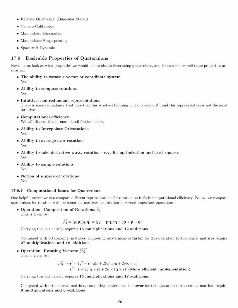
• Relative Orientation (Binocular Stereo)

• Camera Calibration

• Manipulator Kinematics

• Manipulator Fingerprinting

• Spacecraft Dynamics

17.9 Desirable Properties of Quaternions

Next, let us look at what propreties we would like to obtain from using quaternions, and let us see how well these properties aresatisfied:

• The ability to rotate a vector or coordinate systemYes!

• Ability to compose rotationsYes!

• Intuitive, non-redundant representationsThere is some redundancy (but note that this is solved by using unit quaternions!), and this representation is not the mostintuitive.

• Computational efficiencyWe will discuss this in more detail further below.

• Ability to Interpolate OrientationsYes!

• Ability to average over rotationsYes!

• Ability to take derivative w.r.t. rotation - e.g. for optimization and least squaresYes!

• Ability to sample rotationsYes!

• Notion of a space of rotationsYes!

17.9.1 Computational Issues for Quaternions

One helpful metric we can compare different representations for rotation on is their computational efficiency. Below, we comparequaternions for rotation with orthonormal matrices for rotation in several important operations:

• Operation: Composition of Rotations:opoq

This is given by:

opoq = (p,p)(q,q) = (pp− pq, pq + qp + p× q)

Carrying this out naively requires 16 multiplications and 12 additions.

Compared with orthonormal matrices, composing quaternions is faster for this operation (orthonormal matrices require27 multiplications and 18 additions.

• Operation: Rotating Vectors:oqoroq∗

This is given by:

oqoroq∗→r′ = (q2 − r · q)r + 2(q · r)q + 2q(q× r)

r′ = r + 2q(q× r) + 2q× (q× r) (More efficient implementation)

Carrying this out naively requires 15 multiplications and 12 additions.

Compared with orthonormal matrices, composing quaternions is slower for this operation (orthonormal matrices require9 multiplications and 6 additions.

126

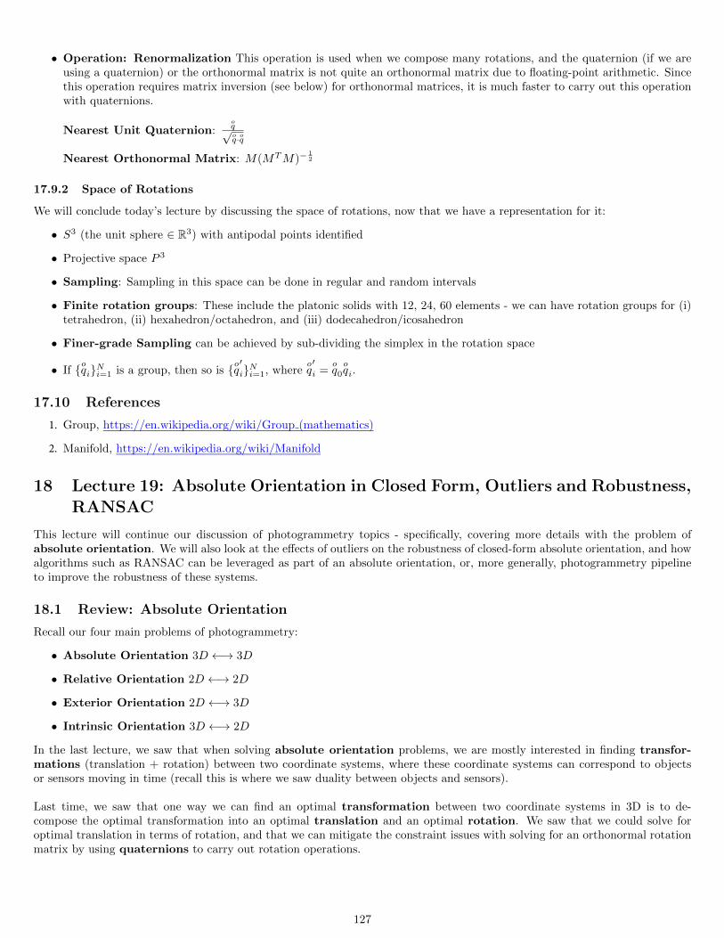
• Operation: Renormalization This operation is used when we compose many rotations, and the quaternion (if we areusing a quaternion) or the orthonormal matrix is not quite an orthonormal matrix due to floating-point arithmetic. Sincethis operation requires matrix inversion (see below) for orthonormal matrices, it is much faster to carry out this operationwith quaternions.

Nearest Unit Quaternion:oq√oq·oq

Nearest Orthonormal Matrix: M(MTM)−12

17.9.2 Space of Rotations

We will conclude today’s lecture by discussing the space of rotations, now that we have a representation for it:

• S3 (the unit sphere ∈ R3) with antipodal points identified

• Projective space P 3

• Sampling: Sampling in this space can be done in regular and random intervals

• Finite rotation groups: These include the platonic solids with 12, 24, 60 elements - we can have rotation groups for (i)tetrahedron, (ii) hexahedron/octahedron, and (iii) dodecahedron/icosahedron

• Finer-grade Sampling can be achieved by sub-dividing the simplex in the rotation space

• If oqiNi=1 is a group, then so is oq′iNi=1, where

oq′i =

oq0oqi.

17.10 References

1. Group, https://en.wikipedia.org/wiki/Group (mathematics)

2. Manifold, https://en.wikipedia.org/wiki/Manifold

18 Lecture 19: Absolute Orientation in Closed Form, Outliers and Robustness,RANSAC

This lecture will continue our discussion of photogrammetry topics - specifically, covering more details with the problem ofabsolute orientation. We will also look at the effects of outliers on the robustness of closed-form absolute orientation, and howalgorithms such as RANSAC can be leveraged as part of an absolute orientation, or, more generally, photogrammetry pipelineto improve the robustness of these systems.

18.1 Review: Absolute Orientation

Recall our four main problems of photogrammetry:

• Absolute Orientation 3D ←→ 3D

• Relative Orientation 2D ←→ 2D

• Exterior Orientation 2D ←→ 3D

• Intrinsic Orientation 3D ←→ 2D

In the last lecture, we saw that when solving absolute orientation problems, we are mostly interested in finding transfor-mations (translation + rotation) between two coordinate systems, where these coordinate systems can correspond to objectsor sensors moving in time (recall this is where we saw duality between objects and sensors).

Last time, we saw that one way we can find an optimal transformation between two coordinate systems in 3D is to de-compose the optimal transformation into an optimal translation and an optimal rotation. We saw that we could solve foroptimal translation in terms of rotation, and that we can mitigate the constraint issues with solving for an orthonormal rotationmatrix by using quaternions to carry out rotation operations.

127

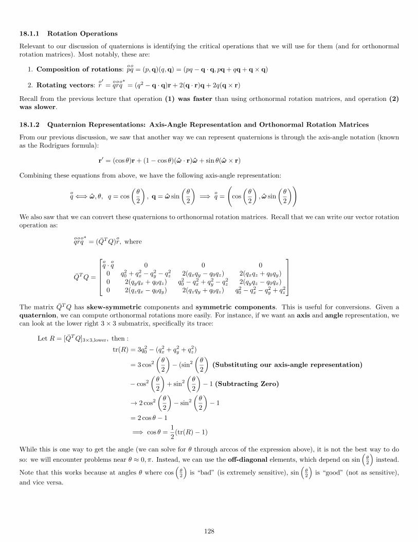
18.1.1 Rotation Operations

Relevant to our discussion of quaternions is identifying the critical operations that we will use for them (and for orthonormalrotation matrices). Most notably, these are:

1. Composition of rotations:opoq = (p,q)(q,q) = (pq − q · q, pq + qq + q× q)

2. Rotating vectors:or′

=oqoroq∗

= (q2 − q · q)r + 2(q · r)q + 2q(q× r)

Recall from the previous lecture that operation (1) was faster than using orthonormal rotation matrices, and operation (2)was slower.

18.1.2 Quaternion Representations: Axis-Angle Representation and Orthonormal Rotation Matrices

From our previous discussion, we saw that another way we can represent quaternions is through the axis-angle notation (knownas the Rodrigues formula):

r′ = (cos θ)r + (1− cos θ)(ω · r)ω + sin θ(ω × r)

Combining these equations from above, we have the following axis-angle representation:

oq ⇐⇒ ω, θ, q = cos

(θ

2

), q = ω sin

(θ

2

)=⇒ o

q =

(cos

(θ

2

), ω sin

(θ

2

))

We also saw that we can convert these quaternions to orthonormal rotation matrices. Recall that we can write our vector rotationoperation as:

oqoroq∗

= (QTQ)or, where

QTQ =

oq · oq 0 0 0

0 q20 + q2

x − q2y − q2

z 2(qxqy − q0qz) 2(qxqz + q0qy)0 2(qyqx + q0qz) q2

0 − q2x + q2

y − q2z 2(qyqz − q0qx)

0 2(qzqx − q0qy) 2(qzqy + q0qz) q20 − q2

x − q2y + q2

z

The matrix QTQ has skew-symmetric components and symmetric components. This is useful for conversions. Given aquaternion, we can compute orthonormal rotations more easily. For instance, if we want an axis and angle representation, wecan look at the lower right 3× 3 submatrix, specifically its trace:

Let R = [QTQ]3×3,lower, then :

tr(R) = 3q20 − (q2

x + q2y + q2

z)

= 3 cos2

(θ

2

)− (sin2

(θ

2

)(Substituting our axis-angle representation)

− cos2

(θ

2

)+ sin2

(θ

2

)− 1 (Subtracting Zero)

→ 2 cos2

(θ

2

)− sin2

(θ

2

)− 1

= 2 cos θ − 1

=⇒ cos θ =1

2(tr(R)− 1)

While this is one way to get the angle (we can solve for θ through arccos of the expression above), it is not the best way to do

so: we will encounter problems near θ ≈ 0, π. Instead, we can use the off-diagonal elements, which depend on sin(θ2

)instead.

Note that this works because at angles θ where cos(θ2

)is “bad” (is extremely sensitive), sin

(θ2

)is “good” (not as sensitive),

and vice versa.

128

18.2 Quaternion Transformations/Conversions

Next, let us focus on how we can convert between quaternions and orthonormal rotation matrices. Given a 3 × 3 orthonormalrotation matrix r, we can compute sums and obtain the following system of equations:

1 + r11 + r22 + r33 = 4q20

1 + r11 − r22 − r33 = 4q2x

1− r11 + r22 − r33 = 4q2y

1− r11 − r22 + r33 = 4q2z

This equation can be solved by taking square roots, but due to the number of solutions (8 by Bezout’s theorem, allowing for theflipped signs of quaternions, we should not use this set of equations alone to find the solution).

Instead, we can compute these equations, evaluate them, take the largest for numerical accuracy, arbitrarily select to usethe positive version (since there is sign ambiguity with the signs of the quaternions), and solve for this. We will call this selectedrighthand side qi.

For off-digaonals, which have symmetric and non-symmetric components, we derive the following equations:

r32 − r23 = 4q0qx

r13 − r31 = 4q0qy

r21 − r12 = 4q0qx

r21 + r12 = 4qxqy

r32 + r23 = 4qyqz

r13 + r31 = 4qzqz

Adding/subtracting off-diagonals give us 6 relations, of which we only need 3 (since we have 1 relation from the diagonals). Forinstance, if we have qi = qy, then we pick off-diagonal relations involving qy, and we solve the four equations given by:

1− r11 + r22 − r33 = 4q2y

r13 − r31 = 4q0qy

r32 + r23 = 4qyqz

r13 + r31 = 4qzqz

This system of four equations gives us a direct way of going from quaternions to an orthonormal rotation matrix. Note that thiscould be 9 numbers that could be noisy, and we want to make sure we have best fits.

18.3 Transformations: Incorporating Scale

Thus far, for our problem of absolute orientation, we have considered transformations between two coordinate systems of beingcomposed of translation and rotation. This is often sufficient, but in some applications and domains, such as satellite imagingfr topographic reconstruction, we may be able to better describe these transformations taking account not only translation androtation, but also scaling.

Taking scaling into account, we can write the relationship between two point clouds corresponding to two different coordi-nate systems as:

r′r = sR(r′l)

Where rotation is again given by R ∈ SO(3), and the scaling factor is given by s ∈ R+ (where R+ ∆= x : x ∈ R , x > 0. Recall

that r′r and r′l are the centroid-subtracted variants of the point clouds in both frames of reference.

18.3.1 Solving for Scaling Using Least Squares: Asymmetric Case

As we did before, we can write this as a least-squares problem over the scaling parameter s:

mins

n∑i=1

||r′r,i − sR(r′l,i)||22

129

As we did for translation and rotation, we can solve for an optimal scaling parameter:

s∗ = arg mins

n∑i=1

||r′r,i − sR(r′l,i)||22

= arg mins

n∑i=1

(||r′r,i||22

)− 2s

n∑i=1

(r′r,iR(r′l,i)

)+ s2

n∑i=1

||R(r′l,i)||22

= arg mins

n∑i=1

(||r′r,i||22

)− 2s

n∑i=1

(r′r,iR(r′l,i)

)+ s2

n∑i=1

||r′l,i||22 (Rotation preserves vector lengths)

Next, let us define the following terms:

1. sr∆=∑ni=1

(||r′r,i||22

)2. D

∆=∑ni=1

(r′r,iR(r′l,i)

)3. sl

∆=∑ni=1 ||r′l,i||22

Then we can write this objective for the optimal scaling factor s∗ as:

s∗ = arg minsJ(s)

∆= sr − 2sD + s2sl

Since this is an unconstrained optimization problem, we can solve this by taking the derivative w.r.t. s and setting it equal to 0:

dJ(s)

ds=

d

ds

(sr − 2sD + s2sl

)= 0

= −2D + s2sl = 0 =⇒ s =D

sl

As we also saw with rotation, this does not give us an exact answer without finding the orthonormal matrix R, but now we areable to remove scale factor and back-solve for it later using our optimal rotation.

18.3.2 Issues with Symmetry

Symmetry question: What if instead of going from the left coordinate system to the right one, we decided to go from rightto left? In theory, this should be possible: we should be able to do this simply by negating translation and inverting ourrotation and scaling terms. But in general, doing this in practice with our OLS approach above does not lead to sinverse = 1

s- i.e. inverting the optimal scale factor does not give us the scale factor for the reverse problem.

Intuitively, this is the case because the version of OLS we used above “cheats” and tries to minimize error by shriking thescale by more than it should be shrunk. This occurs because it brings the points closer together, thereby minimizing, on average,the error term. Let us look at an alternative formulation for our error term that accounts for this optimization phenomenon.

18.3.3 Solving for Scaling Using Least Squares: Symmetric Case

Let us instead write our objective as:

ei =1√sr′r,i =

√sR(r′l,i)

Then we can write our objective and optimization problem over scale as:

s∗ = arg mins

n∑i=1

|| 1√sr′r,i −

√sR(r′l,i)||22

= arg mins

n∑i=1

(1

s||r′r,i||22

)− 2

n∑i=1

(r′r,iR(r′l,i)

)+ s

n∑i=1

||R(r′l,i)||22

= arg mins

1

s

n∑i=1

(||r′r,i||22

)− 2

n∑i=1

(r′r,iR(r′l,i)

)+ s

n∑i=1

||r′l,i||22 (Rotation preserves vector lengths)

We then take the same definitions for these terms that we did above:

130

1. sr∆=∑ni=1

(||r′r,i||22

)2. D

∆=∑ni=1

(r′r,iR(r′l,i)

)3. sl

∆=∑ni=1 ||r′l,i||22

Then, as we did for the asymmetric OLS case, we can write this objective for the optimal scaling factor s∗ as:

s∗ = arg minsJ(s)

∆=

1

ssr − 2D + ssl

Since this is an unconstrained optimization problem, we can solve this by taking the derivative w.r.t. s and setting it equal to 0:

dJ(s)

ds=

d

ds

(1

ssr − 2D + ssl

)= 0

= − 1

s2sr + sl = 0 =⇒ s2 =

slsr

Therefore, we can see that going in the reverse direction preserves this inverse (you can verify this mathematically and intu-itively by simply setting r′r,i ↔ r′l,i ∀ i ∈ 1, ..., n and noting that you will get s2

inverse = srsl

). Since this method better preservessymmetry, it is preferred.

Intuition: Since s no longer depends on correspondences (matches between points in the left and right point clouds), thenthe scale simply becomes the ratio of the point cloud sizes in both coordinate systems (note that sl and sr correspond to thesummed vector lengths of the centroid-subtracted point clouds, which means they reflect the variance/spread/size of the pointcloud in their respective coordinate systems.

We can deal with translation and rotation in a correspondence-free way, while also allowing for us to decouple rotation. Let usalso look at solving rotation, which is covered in the next section.

18.4 Solving for Optimal Rotation in Absolute Orientation

Recall for rotation (see lecture 18 for details) that we switched from optimizing over orthonormal rotation matrices to opti-mizing over quaternions due to the lessened number of optimization constraints that we must adhere to. With our quaternionoptimization formulation, our problem becomes:

maxoq

oqTNoq, subject to

oqT oq = 1

If this were an unconstrained optimization problem, we could solve by taking the derivative of this objective w.r.t. our quaternionoq and setting it equal to zero. Note the following helpful identities with matrix and vector calculus:

1. dda (a · b) = b

2. dda (aTMb) = 2Mb

However, since we are working with quaternions, we must take this constraint into account. We saw in lecture 18 that we didthis with using Lagrange Multiplier - in this lecture it is also possible to take this specific kind of vector length constraintinto account using Rayleigh Quotients.

What are Rayleigh Quotients? The intuitive idea behind them: How do I prevent my parameters from becoming toolarge) positive or negative) or too small (zero)? We can accomplish this by dividing our objective by our parameters, in thiscase our constraint. In this case, with the Rayleigh Quotient taken into account, our objective becomes:

oqTNoq

oqT oq

Recall that N∆=

n∑i=1

RTl,iRr,i

131

How do we solve this? Since this is now an unconstrained optimization problem, we can solve this simply using the rules ofcalculus:

J(oq)

∆==

oqTNoq

oqT oq

dJ(oq)

doq

=d

doq

oqTNoq

oqT oq

= 0

=

d

doq(oqTNoq)oqT oq − o

qTNoq ddoq(oqT oq)

(oqT oq)2

= 0

=2N

oq

oqT oq− 2

oq

(oqT oq)2

(oqTNoq) = 0

From here, we can write this first order condition result as:

Noq =

oqTNoq

oqT oq

oq

Note thatoqTNoq

oqT oq∈ R (this is our objective). Therefore, we are searching for a vector of quaternion coefficients such applying the

rotation matrix to this vector simply produces a scalar multiple of it - i.e. an eigenvector of the matrix N . Letting λ∆=

oqTNoq

oqT oq

,

then this simply becomes Noq = λ

oq. Since this optimization problem is a maximization problem, this means that we can pick

the eigenvector of N that corresponds to the largest eigenvalue (which in turn maximizes the objective consisting of the

Rayleigh quotientoqTNoq

oqT oq

, which is the eigenvalue.

Even though this quaternion-based optimization approach requires taking this Rayleigh Quotient into account, it is much easierto do this optimization than to solve for orthonormal matrices, which either require a complex Lagrangian (if we solve withLagrange multipliers) or an SVD decomposition from Euclidean space to the SO(3) group (which also happens to be a manifold).

This approach raises a few questions:

• How many correspondences are needed to solve these optimization problems? Recall a correspondence is when we saytwo 3D points in different coordinate systems belong to the same point in 3D space, i.e. the same point observed in twoseparate frames of reference.

• When do these approaches fail?

We cover these two questions in more detail below.

18.4.1 How Many Correspondences Do We Need?

Recall that we are looking for 6 parameters (for translation and rotation) or 7 parameters (for translation, rotation, and scaling).Since each correspondence provides three constraints (since we equate the 3-dimensional coordinates of two 3D points in space),assuming non-redundancy, then we can solve this with two correspondences.

Let us start with two correspondences: if we have two objects corresponding to the correspondences of points in the 3D world,then if we rotate one object about axis, we find this does not work, i.e. we have an additional degree of freedom. Note that thedistance between correspondences is fixed.

132

Figure 33: Using two correspondences leads to only satisfying 5 of the 6 needed constraints to solve for translation and rotationbetween two point clouds.

Because we have one more degree of freedom, this accounts for only 5 of the 6 needed constraints to solve for translation androtation, so we need to have at least 3 correspondences.

With 3 correspondences, we get 9 constraints, which leads to some redundancies. We can add more constraints by incor-porating scaling and generalizing the allowable transformations between the two coordinate systems to be the generalizedlinear transformation - this corresponds to allowing non-orthonormal rotation transformations. This approach gives us 9unknowns! a11 a12 a13

a21 a22 a23

a31 a32 a33

xyz

+

a14

a24

a34

But we also have to account for translation, which gives us another 3 unknowns, giving us 12 in total and therefore requiring atleast 4 non-redundant correspondences in order to compute the full general linear transformation. Note that this doesn’t haveany constraints as well!

On a practical note, this is often not needed, especially for finding the absolute orientation between two cameras, becauseoftentimes the only transformations that need to be considered due to the design constraints of the system (e.g. an autonomouscar with two lidar systems, one on each side) are translation and rotation.

18.4.2 When do These Approaches Fail?

These approaches can fail when we do not have enough correspondences. In this case, the matrix N will become singular, andwill produce eigenvalues of zero. A more interesting failure case occurs when the points of one or both of the point clouds arecoplanar. Recall that we solve for the eigenvalues of a matrix (N in this case) using the characteristic equation given by:

Characteristic Equation : det |N − λI| = 0

Leads to 4th-order polynomial : λ4 + c3λ3 + c2λ

2 + c1λ+ c0 = 0

Recall that our matrix N composed of the data has some special properties:

1. c3 = tr(N) = 0 (This is actually a great feature, since usually the first step in solving 4th-order polynomial systems iseliminating the third-order term).

2. c2 = 2tr(MTM), where M is defined as the sum of dyadic products between the points in the point clouds:

M∆=

n∑i=1

r′l,ir′r,iT

∈ R3×3

3. c1 = 8 det |M |

4. c0 = det |N |

What happens if det |M | = 0, i.e. the matrix M is singular? Then using the formulas above we must have that the coefficientc1 = 0. Then this problem reduces to:

λ4 + c2λ2 + c0 = 0

This case corresponds to a special geometric case/configuration of the point clouds - specifically, when points are coplanar.

133

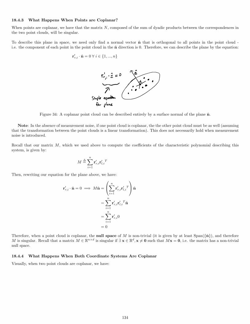
18.4.3 What Happens When Points are Coplanar?

When points are coplanar, we have that the matrix N , composed of the sum of dyadic products between the correspondences inthe two point clouds, will be singular.

To describe this plane in space, we need only find a normal vector n that is orthogonal to all points in the point cloud -i.e. the component of each point in the point cloud in the n direction is 0. Therefore, we can describe the plane by the equation:

r′r,i · n = 0 ∀ i ∈ 1, ..., n

Figure 34: A coplanar point cloud can be described entirely by a surface normal of the plane n.

Note: In the absence of measurement noise, if one point cloud is coplanar, the the other point cloud must be as well (assumingthat the transformation between the point clouds is a linear transformation). This does not necessarily hold when measurementnoise is introduced.

Recall that our matrix M , which we used above to compute the coefficients of the characteristic polynomial describing thissystem, is given by:

M∆=

n∑i=1

r′r,ir′l,iT

Then, rewriting our equation for the plane above, we have:

r′r,i · n = 0 =⇒ M n =

n∑i=1

r′r,ir′l,iT

n

=n∑i=1

r′r,ir′l,iT n

=n∑i=1

r′r,i0

= 0

Therefore, when a point cloud is coplanar, the null space of M is non-trivial (it is given by at least Span(n), and thereforeM is singular. Recall that a matrix M ∈ Rn×d is singular if ∃ x ∈ Rd,x 6= 0 such that Mx = 0, i.e. the matrix has a non-trivialnull space.

18.4.4 What Happens When Both Coordinate Systems Are Coplanar

Visually, when two point clouds are coplanar, we have:

134

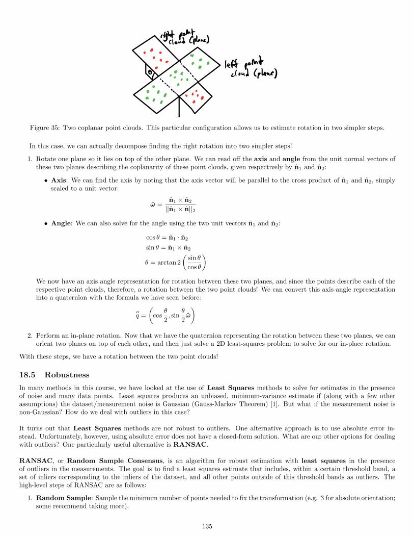
Figure 35: Two coplanar point clouds. This particular configuration allows us to estimate rotation in two simpler steps.

In this case, we can actually decompose finding the right rotation into two simpler steps!

1. Rotate one plane so it lies on top of the other plane. We can read off the axis and angle from the unit normal vectors ofthese two planes describing the coplanarity of these point clouds, given respectively by n1 and n2:

• Axis: We can find the axis by noting that the axis vector will be parallel to the cross product of n1 and n2, simplyscaled to a unit vector:

ω =n1 × n2

||n1 × n||2

• Angle: We can also solve for the angle using the two unit vectors n1 and n2:

cos θ = n1 · n2

sin θ = n1 × n2

θ = arctan 2

(sin θ

cos θ

)We now have an axis angle representation for rotation between these two planes, and since the points describe each of therespective point clouds, therefore, a rotation between the two point clouds! We can convert this axis-angle representationinto a quaternion with the formula we have seen before:

oq =

(cos

θ

2, sin

θ

2ω

)2. Perform an in-plane rotation. Now that we have the quaternion representing the rotation between these two planes, we can

orient two planes on top of each other, and then just solve a 2D least-squares problem to solve for our in-place rotation.

With these steps, we have a rotation between the two point clouds!

18.5 Robustness

In many methods in this course, we have looked at the use of Least Squares methods to solve for estimates in the presenceof noise and many data points. Least squares produces an unbiased, minimum-variance estimate if (along with a few otherassumptions) the dataset/measurement noise is Gaussian (Gauss-Markov Theorem) [1]. But what if the measurement noise isnon-Gaussian? How do we deal with outliers in this case?

It turns out that Least Squares methods are not robust to outliers. One alternative approach is to use absolute error in-stead. Unfortunately, however, using absolute error does not have a closed-form solution. What are our other options for dealingwith outliers? One particularly useful alternative is RANSAC.

RANSAC, or Random Sample Consensus, is an algorithm for robust estimation with least squares in the presenceof outliers in the measurements. The goal is to find a least squares estimate that includes, within a certain threshold band, aset of inliers corresponding to the inliers of the dataset, and all other points outside of this threshold bands as outliers. Thehigh-level steps of RANSAC are as follows:

1. Random Sample: Sample the minimum number of points needed to fix the transformation (e.g. 3 for absolute orientation;some recommend taking more).

135

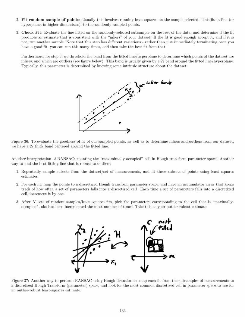
2. Fit random sample of points: Usually this involves running least squares on the sample selected. This fits a line (orhyperplane, in higher dimensions), to the randomly-sampled points.

3. Check Fit: Evaluate the line fitted on the randomly-selected subsample on the rest of the data, and determine if the fitproduces an estimate that is consistent with the “inliers” of your dataset. If the fit is good enough accept it, and if it isnot, run another sample. Note that this step has different variations - rather than just immediately terminating once youhave a good fit, you can run this many times, and then take the best fit from that.

Furthermore, for step 3, we threshold the band from the fitted line/hyperplane to determine which points of the dataset areinliers, and which are outliers (see figure below). This band is usually given by a 2ε band around the fitted line/hyperplane.Typically, this parameter is determined by knowing some intrinsic structure about the dataset.

Figure 36: To evaluate the goodness of fit of our sampled points, as well as to determine inliers and outliers from our dataset,we have a 2ε thick band centered around the fitted line.

Another interpretation of RANSAC: counting the “maximimally-occupied” cell in Hough transform parameter space! Anotherway to find the best fitting line that is robust to outliers:

1. Repeatedly sample subsets from the dataset/set of measurements, and fit these subsets of points using least squaresestimates.

2. For each fit, map the points to a discretized Hough transform parameter space, and have an accumulator array that keepstrack of how often a set of parameters falls into a discretized cell. Each time a set of parameters falls into a discretizedcell, increment it by one.

3. After N sets of random samples/least squares fits, pick the parameters corresponding to the cell that is “maximally-occupied”, aka has been incremented the most number of times! Take this as your outlier-robust estimate.

Figure 37: Another way to perform RANSAC using Hough Transforms: map each fit from the subsamples of measurements toa discretized Hough Transform (parameter) space, and look for the most common discretized cell in parameter space to use foran outlier-robust least-squares estimate.

136

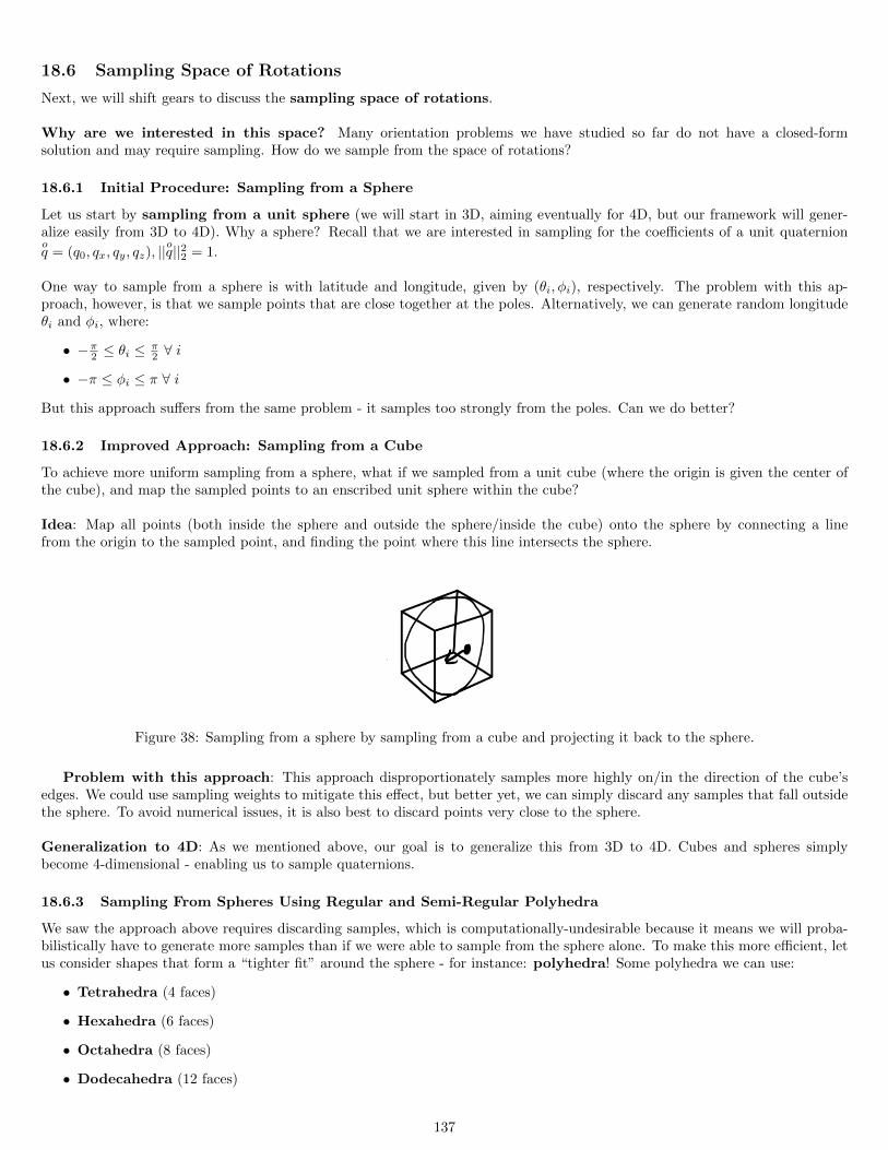
18.6 Sampling Space of Rotations

Next, we will shift gears to discuss the sampling space of rotations.

Why are we interested in this space? Many orientation problems we have studied so far do not have a closed-formsolution and may require sampling. How do we sample from the space of rotations?

18.6.1 Initial Procedure: Sampling from a Sphere

Let us start by sampling from a unit sphere (we will start in 3D, aiming eventually for 4D, but our framework will gener-alize easily from 3D to 4D). Why a sphere? Recall that we are interested in sampling for the coefficients of a unit quaternionoq = (q0, qx, qy, qz), ||

oq||22 = 1.

One way to sample from a sphere is with latitude and longitude, given by (θi, φi), respectively. The problem with this ap-proach, however, is that we sample points that are close together at the poles. Alternatively, we can generate random longitudeθi and φi, where:

• −π2 ≤ θi ≤π2 ∀ i

• −π ≤ φi ≤ π ∀ i

But this approach suffers from the same problem - it samples too strongly from the poles. Can we do better?

18.6.2 Improved Approach: Sampling from a Cube

To achieve more uniform sampling from a sphere, what if we sampled from a unit cube (where the origin is given the center ofthe cube), and map the sampled points to an enscribed unit sphere within the cube?

Idea: Map all points (both inside the sphere and outside the sphere/inside the cube) onto the sphere by connecting a linefrom the origin to the sampled point, and finding the point where this line intersects the sphere.

Figure 38: Sampling from a sphere by sampling from a cube and projecting it back to the sphere.

Problem with this approach: This approach disproportionately samples more highly on/in the direction of the cube’sedges. We could use sampling weights to mitigate this effect, but better yet, we can simply discard any samples that fall outsidethe sphere. To avoid numerical issues, it is also best to discard points very close to the sphere.

Generalization to 4D: As we mentioned above, our goal is to generalize this from 3D to 4D. Cubes and spheres simplybecome 4-dimensional - enabling us to sample quaternions.

18.6.3 Sampling From Spheres Using Regular and Semi-Regular Polyhedra

We saw the approach above requires discarding samples, which is computationally-undesirable because it means we will proba-bilistically have to generate more samples than if we were able to sample from the sphere alone. To make this more efficient, letus consider shapes that form a “tighter fit” around the sphere - for instance: polyhedra! Some polyhedra we can use:

• Tetrahedra (4 faces)

• Hexahedra (6 faces)

• Octahedra (8 faces)

• Dodecahedra (12 faces)

137

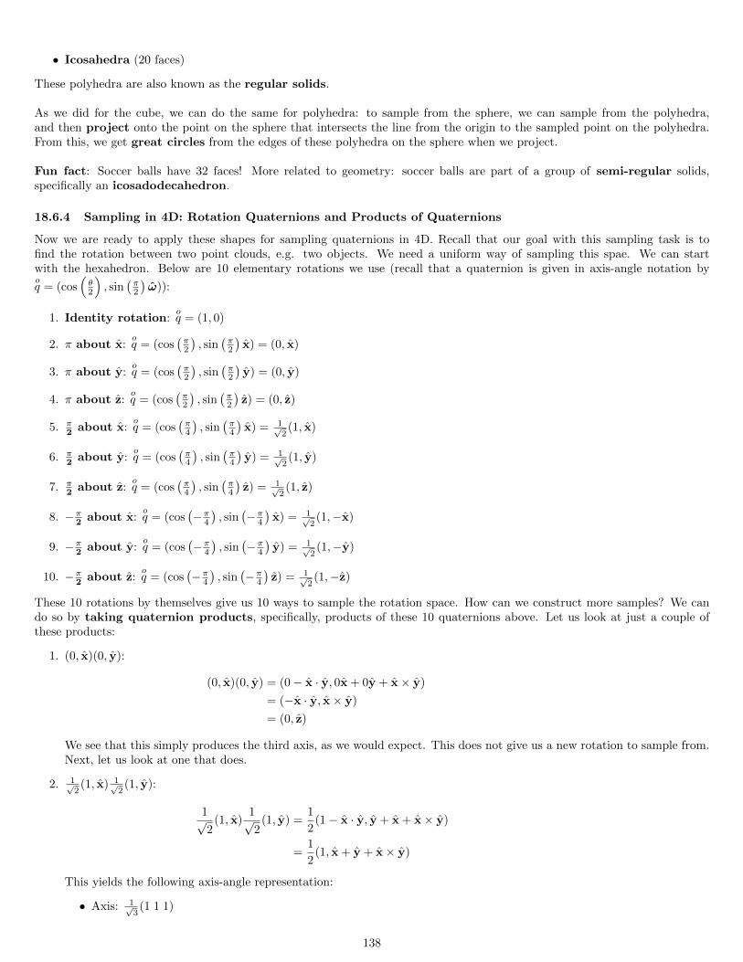
• Icosahedra (20 faces)

These polyhedra are also known as the regular solids.

As we did for the cube, we can do the same for polyhedra: to sample from the sphere, we can sample from the polyhedra,and then project onto the point on the sphere that intersects the line from the origin to the sampled point on the polyhedra.From this, we get great circles from the edges of these polyhedra on the sphere when we project.

Fun fact: Soccer balls have 32 faces! More related to geometry: soccer balls are part of a group of semi-regular solids,specifically an icosadodecahedron.

18.6.4 Sampling in 4D: Rotation Quaternions and Products of Quaternions

Now we are ready to apply these shapes for sampling quaternions in 4D. Recall that our goal with this sampling task is tofind the rotation between two point clouds, e.g. two objects. We need a uniform way of sampling this spae. We can startwith the hexahedron. Below are 10 elementary rotations we use (recall that a quaternion is given in axis-angle notation byoq = (cos

(θ2

), sin

(π2

)ω)):

1. Identity rotation:oq = (1, 0)

2. π about x:oq = (cos

(π2

), sin

(π2

)x) = (0, x)

3. π about y:oq = (cos

(π2

), sin

(π2

)y) = (0, y)

4. π about z:oq = (cos

(π2

), sin

(π2

)z) = (0, z)

5. π2 about x:

oq = (cos

(π4

), sin

(π4

)x) = 1√

2(1, x)

6. π2 about y:

oq = (cos

(π4

), sin

(π4

)y) = 1√

2(1, y)

7. π2 about z:

oq = (cos

(π4

), sin

(π4

)z) = 1√

2(1, z)

8. −π2 about x:oq = (cos

(−π4), sin

(−π4)x) = 1√

2(1,−x)

9. −π2 about y:oq = (cos

(−π4), sin

(−π4)y) = 1√

2(1,−y)

10. −π2 about z:oq = (cos

(−π4), sin

(−π4)z) = 1√

2(1,−z)

These 10 rotations by themselves give us 10 ways to sample the rotation space. How can we construct more samples? We cando so by taking quaternion products, specifically, products of these 10 quaternions above. Let us look at just a couple ofthese products:

1. (0, x)(0, y):

(0, x)(0, y) = (0− x · y, 0x + 0y + x× y)

= (−x · y, x× y)

= (0, z)

We see that this simply produces the third axis, as we would expect. This does not give us a new rotation to sample from.Next, let us look at one that does.

2. 1√2(1, x) 1√

2(1, y):

1√2

(1, x)1√2

(1, y) =1

2(1− x · y, y + x + x× y)

=1

2(1, x + y + x× y)

This yields the following axis-angle representation:

• Axis: 1√3(1 1 1)

138

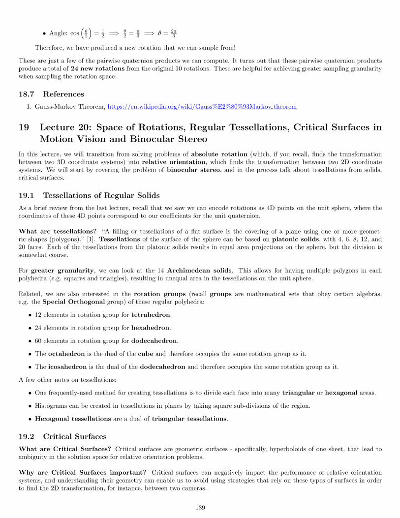
• Angle: cos(θ2

)= 1

2 =⇒ θ2 = π

3 =⇒ θ = 2π3

Therefore, we have produced a new rotation that we can sample from!

These are just a few of the pairwise quaternion products we can compute. It turns out that these pairwise quaternion productsproduce a total of 24 new rotations from the original 10 rotations. These are helpful for achieving greater sampling granularitywhen sampling the rotation space.

18.7 References

1. Gauss-Markov Theorem, https://en.wikipedia.org/wiki/Gauss%E2%80%93Markov theorem

19 Lecture 20: Space of Rotations, Regular Tessellations, Critical Surfaces inMotion Vision and Binocular Stereo

In this lecture, we will transition from solving problems of absolute rotation (which, if you recall, finds the transformationbetween two 3D coordinate systems) into relative orientation, which finds the transformation between two 2D coordinatesystems. We will start by covering the problem of binocular stereo, and in the process talk about tessellations from solids,critical surfaces.

19.1 Tessellations of Regular Solids

As a brief review from the last lecture, recall that we saw we can encode rotations as 4D points on the unit sphere, where thecoordinates of these 4D points correspond to our coefficients for the unit quaternion.

What are tessellations? “A filling or tessellations of a flat surface is the covering of a plane using one or more geomet-ric shapes (polygons).” [1]. Tessellations of the surface of the sphere can be based on platonic solids, with 4, 6, 8, 12, and20 faces. Each of the tessellations from the platonic solids results in equal area projections on the sphere, but the division issomewhat coarse.

For greater granularity, we can look at the 14 Archimedean solids. This allows for having multiple polygons in eachpolyhedra (e.g. squares and triangles), resulting in unequal area in the tessellations on the unit sphere.

Related, we are also interested in the rotation groups (recall groups are mathematical sets that obey certain algebras,e.g. the Special Orthogonal group) of these regular polyhedra:

• 12 elements in rotation group for tetrahedron.

• 24 elements in rotation group for hexahedron.

• 60 elements in rotation group for dodecahedron.

• The octahedron is the dual of the cube and therefore occupies the same rotation group as it.

• The icosahedron is the dual of the dodecahedron and therefore occupies the same rotation group as it.

A few other notes on tessellations:

• One frequently-used method for creating tessellations is to divide each face into many triangular or hexagonal areas.

• Histograms can be created in tessellations in planes by taking square sub-divisions of the region.

• Hexagonal tessellations are a dual of triangular tessellations.

19.2 Critical Surfaces

What are Critical Surfaces? Critical surfaces are geometric surfaces - specifically, hyperboloids of one sheet, that lead toambiguity in the solution space for relative orientation problems.

Why are Critical Surfaces important? Critical surfaces can negatively impact the performance of relative orientationsystems, and understanding their geometry can enable us to avoid using strategies that rely on these types of surfaces in orderto find the 2D transformation, for instance, between two cameras.

139

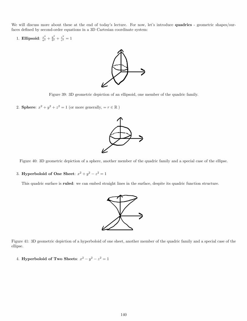
We will discuss more about these at the end of today’s lecture. For now, let’s introduce quadrics - geometric shapes/sur-faces defined by second-order equations in a 3D Cartesian coordinate system:

1. Ellipsoid: x2

a2 + y2

b2 + z2

c2 = 1

Figure 39: 3D geometric depiction of an ellipsoid, one member of the quadric family.

2. Sphere: x2 + y2 + z2 = 1 (or more generally, = r ∈ R )

Figure 40: 3D geometric depiction of a sphere, another member of the quadric family and a special case of the ellipse.

3. Hyperboloid of One Sheet: x2 + y2 − z2 = 1

This quadric surface is ruled: we can embed straight lines in the surface, despite its quadric function structure.

Figure 41: 3D geometric depiction of a hyperboloid of one sheet, another member of the quadric family and a special case of theellipse.

4. Hyperboloid of Two Sheets: x2 − y2 − z2 = 1

140

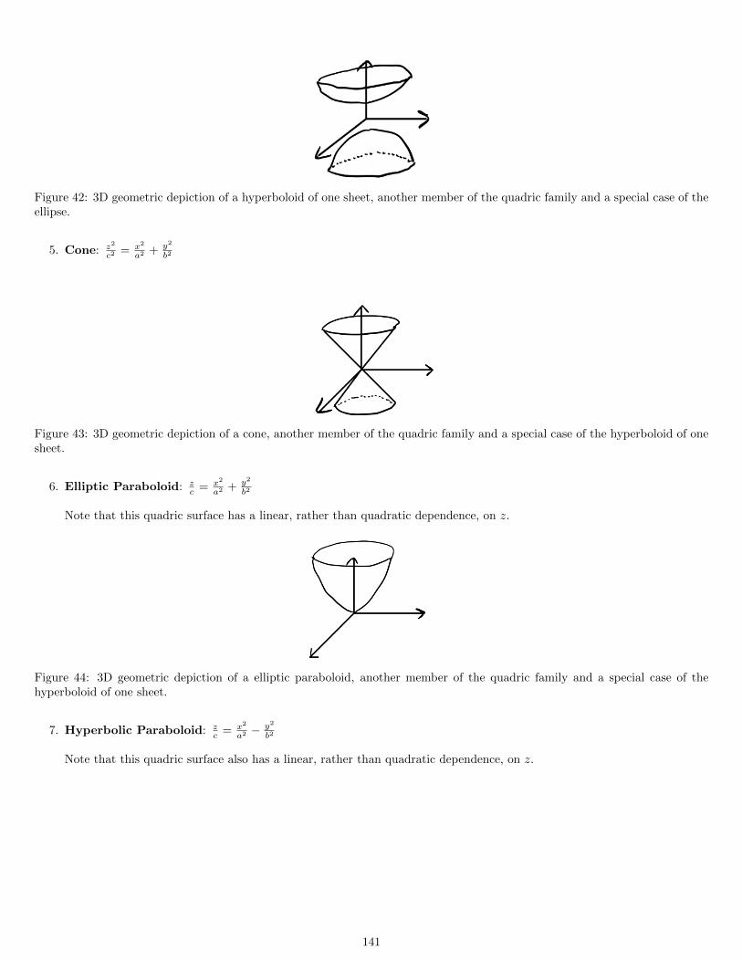
Figure 42: 3D geometric depiction of a hyperboloid of one sheet, another member of the quadric family and a special case of theellipse.

5. Cone: z2

c2 = x2

a2 + y2

b2

Figure 43: 3D geometric depiction of a cone, another member of the quadric family and a special case of the hyperboloid of onesheet.

6. Elliptic Paraboloid: zc = x2

a2 + y2

b2

Note that this quadric surface has a linear, rather than quadratic dependence, on z.

Figure 44: 3D geometric depiction of a elliptic paraboloid, another member of the quadric family and a special case of thehyperboloid of one sheet.

7. Hyperbolic Paraboloid: zc = x2

a2 −y2

b2

Note that this quadric surface also has a linear, rather than quadratic dependence, on z.

141

Figure 45: 3D geometric depiction of a hyperbolic paraboloid, another member of the quadric family and a special case of thehyperboloid of one sheet.

Another special case is derived through planes. You may be wondering - how can we have a quadratic structure from planes? Wecan derive a surface with quadratic terms by considering the intersection of two planes. This intersection of planes is computedanalytically as a product of two linear equations, resulting in a quadratic equation.

19.3 Relative Orientation and Binocular Stereo

Problem of interest: Computing 3D from 3D using two cameras - a problem known as binocular stereo. We found thisproblem was easy to solve if the geometry of the two cameras, in this case known as the two-view geometry, is known andcalibrated (usually this results in finding a calibration matrix K). To achieve high-performing binocular stereo systems, we needto find the relative orientation between the two cameras. A few other notes on this:

• Calibration is typically for binocular stereo using baseline calibration.

• Recall that like absolute orientation, we have duality in te problems we solve: we are able to apply the same machinevision framework regardless of “if the camera moved of it the world moved”.

• Therefore, the dual problem to binocular stereo is structure from motion, also known as Visual Odometry (VO).This involves finding transformations over time from camera (i.e. one moving camera at different points in time).

19.3.1 Binocular Stereo

Recall that our goal with binocular stereo is to find the translation (known as the baseline, given by b ∈ R3. The diagrambelow illustrates our setup with two cameras, points in the world, and the translation between the two cameras given as thisaforementioned baseline b.

Figure 46: Binocular stereo system set up. For this problem, recall that one of our objectives is to measure the translation, orbaseline, between the two cameras.

When we search for correspondences, we need only search along a line, which gives us a measure of binocular disparitythat we can then use to measure distance between the cameras.

142

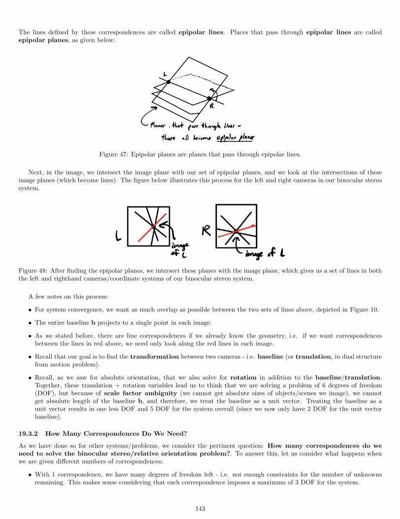
The lines defined by these correspondences are called epipolar lines. Places that pass through epipolar lines are calledepipolar planes, as given below:

Figure 47: Epipolar planes are planes that pass through epipolar lines.

Next, in the image, we intersect the image plane with our set of epipolar planes, and we look at the intersections of theseimage planes (which become lines). The figure below illustrates this process for the left and right cameras in our binocular stereosystem.

Figure 48: After finding the epipolar planes, we intersect these planes with the image plane, which gives us a set of lines in boththe left and righthand cameras/coordinate systems of our binocular stereo system.

A few notes on this process:

• For system convergence, we want as much overlap as possible between the two sets of lines above, depicted in Figure 10.

• The entire baseline b projects to a single point in each image.

• As we stated before, there are line correspondences if we already know the geometry, i.e. if we want correspondencesbetween the lines in red above, we need only look along the red lines in each image.

• Recall that our goal is to find the transformation between two cameras - i.e. baseline (or translation, in dual structurefrom motion problem).

• Recall, as we saw for absolute orientation, that we also solve for rotation in addition to the baseline/translation.Together, these translation + rotation variables lead us to think that we are solving a problem of 6 degrees of freedom(DOF), but because of scale factor ambiguity (we cannot get absolute sizes of objects/scenes we image), we cannotget absolute length of the baseline b, and therefore, we treat the baseline as a unit vector. Treating the baseline as aunit vector results in one less DOF and 5 DOF for the system overall (since we now only have 2 DOF for the unit vectorbaseline).

19.3.2 How Many Correspondences Do We Need?

As we have done so for other systems/problems, we consider the pertinent question: How many correspondences do weneed to solve the binocular stereo/relative orientation problem?. To answer this, let us consider what happens whenwe are given different numbers of correspondences:

• With 1 correspondence, we have many degrees of freedom left - i.e. not enough constraints for the number of unknownsremaining. This makes sense considering that each correspondence imposes a maximum of 3 DOF for the system.

143

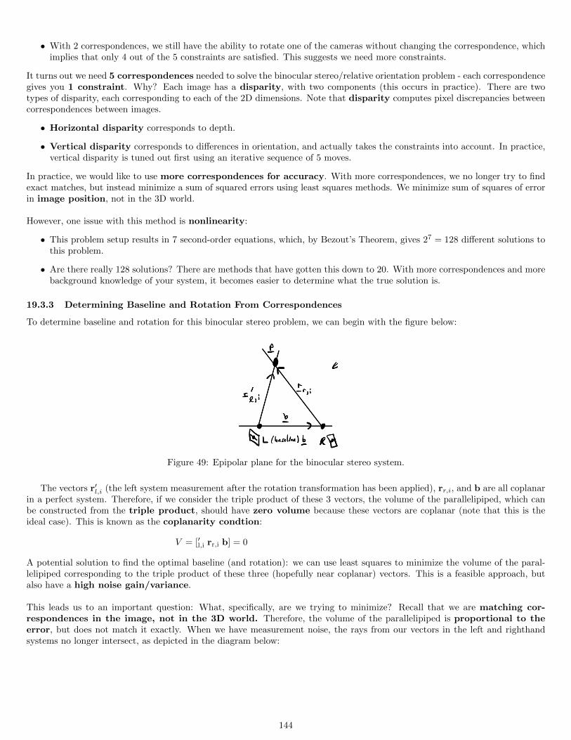
• With 2 correspondences, we still have the ability to rotate one of the cameras without changing the correspondence, whichimplies that only 4 out of the 5 constraints are satisfied. This suggests we need more constraints.

It turns out we need 5 correspondences needed to solve the binocular stereo/relative orientation problem - each correspondencegives you 1 constraint. Why? Each image has a disparity, with two components (this occurs in practice). There are twotypes of disparity, each corresponding to each of the 2D dimensions. Note that disparity computes pixel discrepancies betweencorrespondences between images.

• Horizontal disparity corresponds to depth.

• Vertical disparity corresponds to differences in orientation, and actually takes the constraints into account. In practice,vertical disparity is tuned out first using an iterative sequence of 5 moves.

In practice, we would like to use more correspondences for accuracy. With more correspondences, we no longer try to findexact matches, but instead minimize a sum of squared errors using least squares methods. We minimize sum of squares of errorin image position, not in the 3D world.

However, one issue with this method is nonlinearity:

• This problem setup results in 7 second-order equations, which, by Bezout’s Theorem, gives 27 = 128 different solutions tothis problem.

• Are there really 128 solutions? There are methods that have gotten this down to 20. With more correspondences and morebackground knowledge of your system, it becomes easier to determine what the true solution is.

19.3.3 Determining Baseline and Rotation From Correspondences

To determine baseline and rotation for this binocular stereo problem, we can begin with the figure below:

Figure 49: Epipolar plane for the binocular stereo system.

The vectors r′l,i (the left system measurement after the rotation transformation has been applied), rr,i, and b are all coplanarin a perfect system. Therefore, if we consider the triple product of these 3 vectors, the volume of the parallelipiped, which canbe constructed from the triple product, should have zero volume because these vectors are coplanar (note that this is theideal case). This is known as the coplanarity condtion:

V = [′l,i rr,i b] = 0

A potential solution to find the optimal baseline (and rotation): we can use least squares to minimize the volume of the paral-lelipiped corresponding to the triple product of these three (hopefully near coplanar) vectors. This is a feasible approach, butalso have a high noise gain/variance.

This leads us to an important question: What, specifically, are we trying to minimize? Recall that we are matching cor-respondences in the image, not in the 3D world. Therefore, the volume of the parallelipiped is proportional to theerror, but does not match it exactly. When we have measurement noise, the rays from our vectors in the left and righthandsystems no longer intersect, as depicted in the diagram below:

144

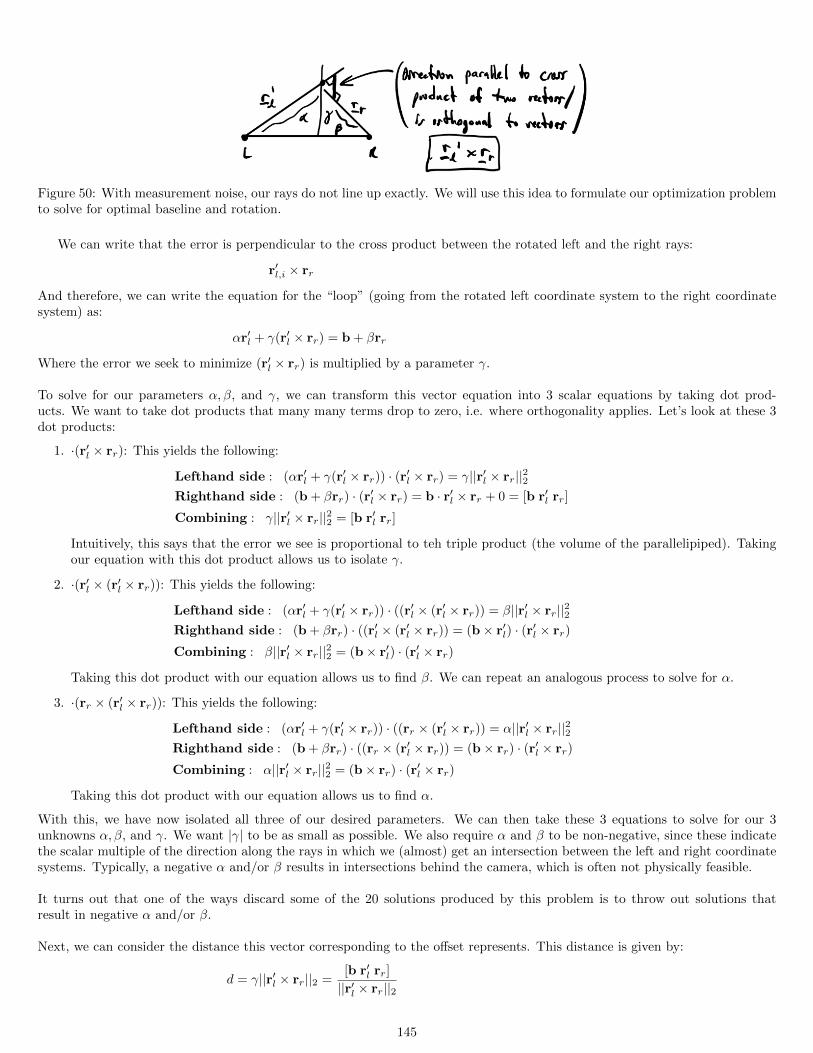
Figure 50: With measurement noise, our rays do not line up exactly. We will use this idea to formulate our optimization problemto solve for optimal baseline and rotation.

We can write that the error is perpendicular to the cross product between the rotated left and the right rays:

r′l,i × rr

And therefore, we can write the equation for the “loop” (going from the rotated left coordinate system to the right coordinatesystem) as:

αr′l + γ(r′l × rr) = b + βrr

Where the error we seek to minimize (r′l × rr) is multiplied by a parameter γ.

To solve for our parameters α, β, and γ, we can transform this vector equation into 3 scalar equations by taking dot prod-ucts. We want to take dot products that many many terms drop to zero, i.e. where orthogonality applies. Let’s look at these 3dot products:

1. ·(r′l × rr): This yields the following:

Lefthand side : (αr′l + γ(r′l × rr)) · (r′l × rr) = γ||r′l × rr||22Righthand side : (b + βrr) · (r′l × rr) = b · r′l × rr + 0 = [b r′l rr]

Combining : γ||r′l × rr||22 = [b r′l rr]

Intuitively, this says that the error we see is proportional to teh triple product (the volume of the parallelipiped). Takingour equation with this dot product allows us to isolate γ.

2. ·(r′l × (r′l × rr)): This yields the following:

Lefthand side : (αr′l + γ(r′l × rr)) · ((r′l × (r′l × rr)) = β||r′l × rr||22Righthand side : (b + βrr) · ((r′l × (r′l × rr)) = (b× r′l) · (r′l × rr)

Combining : β||r′l × rr||22 = (b× r′l) · (r′l × rr)

Taking this dot product with our equation allows us to find β. We can repeat an analogous process to solve for α.

3. ·(rr × (r′l × rr)): This yields the following:

Lefthand side : (αr′l + γ(r′l × rr)) · ((rr × (r′l × rr)) = α||r′l × rr||22Righthand side : (b + βrr) · ((rr × (r′l × rr)) = (b× rr) · (r′l × rr)

Combining : α||r′l × rr||22 = (b× rr) · (r′l × rr)

Taking this dot product with our equation allows us to find α.

With this, we have now isolated all three of our desired parameters. We can then take these 3 equations to solve for our 3unknowns α, β, and γ. We want |γ| to be as small as possible. We also require α and β to be non-negative, since these indicatethe scalar multiple of the direction along the rays in which we (almost) get an intersection between the left and right coordinatesystems. Typically, a negative α and/or β results in intersections behind the camera, which is often not physically feasible.

It turns out that one of the ways discard some of the 20 solutions produced by this problem is to throw out solutions thatresult in negative α and/or β.

Next, we can consider the distance this vector corresponding to the offset represents. This distance is given by:

d = γ||r′l × rr||2 =[b r′l rr]

||r′l × rr||2

145

Closed-Form Solution: Because this is a system involving 5 second-order equations, and the best we can do is reduce thisto a single 5th-order equation, which we do not (yet) have the closed-form solutions to, we cannot solve for this problem inclosed-form. However, we can still solve for it numerically. We can also look at solving this through a weighted least-squaresapproach below.

19.3.4 Solving Using Weighted Least Squares

Because our distance d can get very large without a huge error in image position, d is not representative of our error of interest.However, it is still proportional. We can account for this difference by using a weighting factor wi, which represents the conver-sion factor from 3D error to 2D image error). We will denote the ith weight as wi.

Therefore, incorporating this weighting factor, our least squares optimization problem becomes:

minb,R(·)

n∑i=1

wi[b r′l rr]2, subject to b · b = ||b||22 = 1

How do we solve this? Because wi will change as our candidate solution changes, we will solve this problem iteratively and inan alternating fashion - we will alternate between updated our conversion weights wi and solving for a new objective given therecent update of weights. Therefore, we can write this optimization problem as:

b∗, R∗ = arg minb,||b||22=1,R(·)

n∑i=1

wi[b r′l rr]2

= arg minb,||b||22=1,R(·)

n∑i=1

wi

((rr,i × b) · r′l,i

)2

Intuition for these weights: Loosely, we can think of the weights as being the conversion factor from 3D to 2D error, andtherefore, they can roughly be thought of as w = f

Z , where f is the focal length and Z is the 3D depth.

Now that we have expressed a closed-form solution to this problem, we are ready to build off of the last two lectures andapply our unit quaternions to solve this problem. Note that because we express the points from the left coordinate system in arotated frame of reference (i.e. with the rotation already applied), then we can incorporate the quaternion into this definitionto show how we can solve for our optimal set of parameters given measurements from both systems:

or′l =

oqorloq∗

Then we can solve for this as t:

t = (rr × b) · r′l

=orro

b · oqorloq∗

=orr(

o

boq) · oqorl

=ordo

d · oqorl, whereo

d∆=

o

boq, which we can think of as a product of baseline and rotation.

Recall that our goal here is to find the baselineo

b - this can be found by solving for our quantityo

d and multiplying it on the

righthand side byoq∗:

o

doq∗

=o

boqoq∗

=o

boe =

o

b

(Recall thatoe = (1, 0) =

oqoq∗)

At first glance, it appears we have 8 unknowns, with 5 constraints. But we can add additional constraints to the system to makethe number of constraints equal the number of DOF:

1. Unit quaternions: ||oq||2 =oq · oq = 1

2. Unit baseline: ||o

b||2 =o

b ·o

b = 1

3. Orthogonality ofoq and

o

d:oq ·

o

d = 0

Therefore, with these constraints, we are able to reach a system with 8 constraints. Note that we have more constraints toenforce than with the absolute orientation problem, making the relative orientation problem more difficult to solve.

146

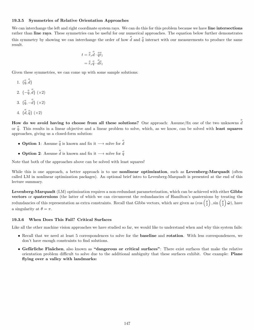
19.3.5 Symmetries of Relative Orientation Approaches

We can interchange the left and right coordinate system rays. We can do this for this problem because we have line intersectionsrather than line rays. These symmetries can be useful for our numerical approaches. The equation below further demonstrates

this symmetry by showing we can interchange the order of howo

d andoq interact with our measurements to produce the same

result.

t =orro

d · oqorl

=orroq ·

o

dorl

Given these symmetries, we can come up with some sample solutions:

1. oq,o

d

2. −oq,o

d (×2)

3. oq,−o

d (×2)

4. o

d,oq (×2)

How do we avoid having to choose from all these solutions? One approach: Assume/fix one of the two unknownso

d

oroq. This results in a linear objective and a linear problem to solve, which, as we know, can be solved with least squares

approaches, giving us a closed-form solution:

• Option 1: Assumeoq is known and fix it −→ solve for

o

d

• Option 2: Assumeo

d is known and fix it −→ solve foroq

Note that both of the approaches above can be solved with least squares!

While this is one approach, a better approach is to use nonlinear optimization, such as Levenberg-Marquadt (oftencalled LM in nonlinear optimization packages). An optional brief intro to Levenberg-Marquadt is presented at the end of thislecture summary.

Levenberg-Marquadt (LM) optimization requires a non-redundant parameterization, which can be achieved with either Gibbsvectors or quaternions (the latter of which we can circumvent the redundancies of Hamilton’s quaternions by treating the

redundancies of this representation as extra constraints. Recall that Gibbs vectors, which are given as (cos(θ2

), sin

(θ2

)ω), have

a singularity at θ = π.

19.3.6 When Does This Fail? Critical Surfaces

Like all the other machine vision approaches we have studied so far, we would like to understand when and why this system fails:

• Recall that we need at least 5 correspondences to solve for the baseline and rotation. With less correspondences, wedon’t have enough constraints to find solutions.

• Gefarliche Flaachen, also known as “dangerous or critical surfaces”: There exist surfaces that make the relativeorientation problem difficult to solve due to the additional ambiguity that these surfaces exhibit. One example: Planeflying over a valley with landmarks:

147

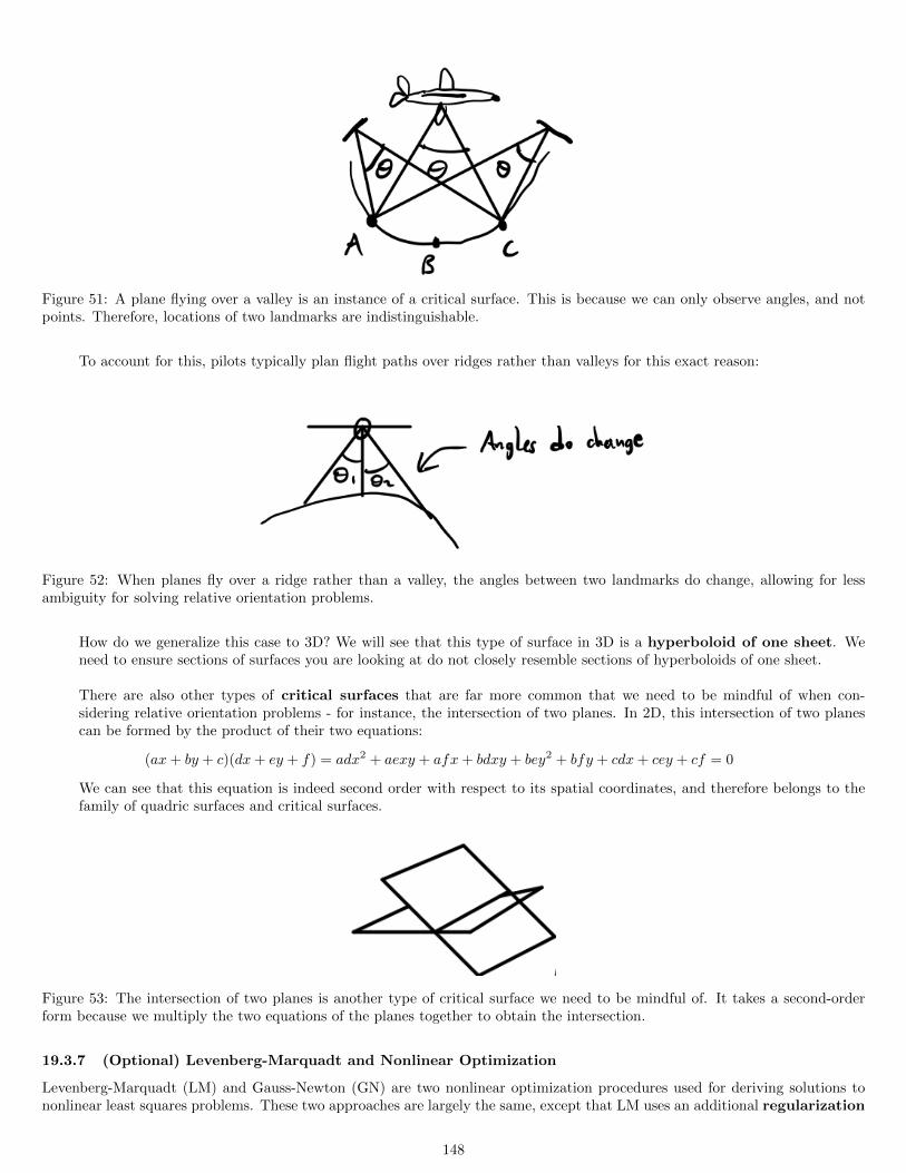
Figure 51: A plane flying over a valley is an instance of a critical surface. This is because we can only observe angles, and notpoints. Therefore, locations of two landmarks are indistinguishable.

To account for this, pilots typically plan flight paths over ridges rather than valleys for this exact reason:

Figure 52: When planes fly over a ridge rather than a valley, the angles between two landmarks do change, allowing for lessambiguity for solving relative orientation problems.

How do we generalize this case to 3D? We will see that this type of surface in 3D is a hyperboloid of one sheet. Weneed to ensure sections of surfaces you are looking at do not closely resemble sections of hyperboloids of one sheet.

There are also other types of critical surfaces that are far more common that we need to be mindful of when con-sidering relative orientation problems - for instance, the intersection of two planes. In 2D, this intersection of two planescan be formed by the product of their two equations:

(ax+ by + c)(dx+ ey + f) = adx2 + aexy + afx+ bdxy + bey2 + bfy + cdx+ cey + cf = 0

We can see that this equation is indeed second order with respect to its spatial coordinates, and therefore belongs to thefamily of quadric surfaces and critical surfaces.

Figure 53: The intersection of two planes is another type of critical surface we need to be mindful of. It takes a second-orderform because we multiply the two equations of the planes together to obtain the intersection.

19.3.7 (Optional) Levenberg-Marquadt and Nonlinear Optimization

Levenberg-Marquadt (LM) and Gauss-Newton (GN) are two nonlinear optimization procedures used for deriving solutions tononlinear least squares problems. These two approaches are largely the same, except that LM uses an additional regularization

148

term to ensure that a solution exists by making the closed-form matrix to invert in the normal equations positive semidefinite.The normal equations, which derive the closed-form solutions for GN and LM, are given by:

1. GN: (J(θ)TJ(θ))−1θ = J(θ)T e(θ) =⇒ θ = (J(θ)TJ(θ))−1J(θ)T e(θ)

2. LM: (J(θ)TJ(θ) + λI)−1θ = J(θ)T e(θ) =⇒ θ = (J(θ)TJ(θ) + λI)−1J(θ)T e(θ)

Where:

• θ is the vector of parameters and our solution point to this nonlinear optimization problem.

• J(θ) is the Jacobian of the nonlinear objective we seek to optimize.

• e(θ) is the residual function of the objective evaluated with the current set of parameters.

Note the λI, or regularization term, in Levenberg-Marquadt. If you’re familiar with ridge regression, LM is effectively ridgeregression/regression with L2 regularization for nonlinear optimization problems. Often, these approaches are solved iterativelyusing gradient descent:

1. GN: θ(t+1) ← θ(t) − α(J(θ(t))TJ(θ(t)))−1J(θ(t))T e(θ(t))

2. LM: θ(t+1) ← θ(t) − α(J(θ(t))TJ(θ(t)) + λI)−1J(θ(t))T e(θ(t))

Where α is the step size, which dictates how quickly the estimates of our approaches update.

19.4 References

1. Tesselation, https://en.wikipedia.org/wiki/Tessellation

20 Lecture 21: Relative Orientation, Binocular Stereo, Structure from Mo-tion, Quadrics, Camera Calibration, Reprojection

Today, we will continue discussing relative orientation, one of our main problems in photogrammetry. We concluded ourprevious lecture with a discussion of critical surfaces - that is, surfaces which make solving the relative rotation problem difficult.In general, these critical surfaces are quadric surfaces, which take the form:

±(x

a

)2

±(y

b

)2

±(z

c

)2

= 1

This form is simple: (i) Centered at the origin, (ii) Axes line up. In general, the form of these quadric surfaces may be morecomplicated, with both linear and constant terms. The signs of these qudratic terms determine the shape, as we saw in theprevious lecture:

1. + + + (ellipsoid)

2. + +− (hyperboloid of one sheet) - this is a class of critical surfaces

3. +−− (hyperboloid of two sheets)

4. −−− (imaginary ellipsoid)

For the solutions to the polynomial R2 + · · ·−R = 0 (the class of hyperboloids of one sheets), the solutions tell us why thesecritical surfaces create solution ambiguity:

1. R = 0: I.e. the solution is on the surface - the origin of the righthand system is on the surface. Two interpretations fromthis; the first is for binocular stereo, and the second is for Structure from Motion (SfM):

(a) Binocular Stereo: The righthand system lies on the surface.

(b) Structure from Motion: In Structure from Motion, we “move ont the surface” in the next time step.

2. R = −b: This solution is the origin of the lefthand system (we move the solution left along the baseline from the righthandsystem to the lefthand system). Two interpretations from this; the first is for binocular stereo, and the second is forStructure from Motion (SfM):

(a) Binocular Stereo: “The surface has to go through both eyes”.

149

(b) Structure from Motion: We must start and end back on the surface.

3. R = kb: Because this system (described by the polynomial in R, then we have no scaling, giving us a solution. Thissuggests that the entire baseline in fact lies on the surface, which in turn suggests:

• This setting/surface configuration is rare.

• This surface is ruled - we can draw lines inscribed in the surface. This suggests that our critical surface is a hyperboloidof one sheet. It turns out that we have two rulings for the hyperboloid at one sheet (i.e. at every point on this surface,we can draw two non-parallel lines through the surface that cross at a point).

Hyperboloids of one sheet, as we saw in the previous lecture, are not the only types of critical surfaces. Intersections of planesare another key type of critical surface, namely because they are much more common in the world than hyperboloids of onesheet. Analytically, the intersection of planes is given by the product of planes:

(a1X + b1Y + c1Z + d1)(a2X + b2Y + c2Z + d2) = 0

This analytic equation describes the intersection of two planes - gives us a quadric surface.

In order for this intersection of planes to not have any constants, one of the planes must be the epipolar plane, whoseimage is a line. The second plane is arbitrary and can take any form.

Practically, we may not run into this problem in this exact analytic form (i.e. a surface that is an exact instance of a hy-perboloid of one sheet), but even as we venture near this condition, the noise amplification factor increases. As it turns out,using a higher/wider Field of View (FOV) helps to mitigate this problem, since as FOV increases, it becomes less and less likelythat the surface we are imaging is locally similar to a critical surface.

One way that we can increase the FOV is through the use of spider heads, which consist of 8 cameras tied together intoa rigid structure. Though it requires calibration between the cameras, we can “stitch” together the images from the 8 camerasinto a single “mosaic image”.

Figure 54: A spider heads apparatus, which is one technique for increasing the FOV, thereby reducing the probability of surfacesresembling critical surfaces.

Next, we will switch our discussion to another of our photogrammetry problems - interior orientation.

20.1 Interior Orientation

Recall that interior orientation was another one of the 4 photogrammetry problems we study, and involves going from 3D (worldcoordinate) to 2D (image coordinates). Specifically, we focus on camera calibration.

Have we already touched on this? Somewhat - with vanishing points. Recall that the goal with vanishing points was tofind (x0, y0, f) using calibration objects. This method:

• Is not very accurate, nor general across different domains/applications

• Does not take into account radial distortion, which we need to take into account for high-quality imaging such as aerialphotography.

What is radial distortion? We touch more on this in the following section.

150

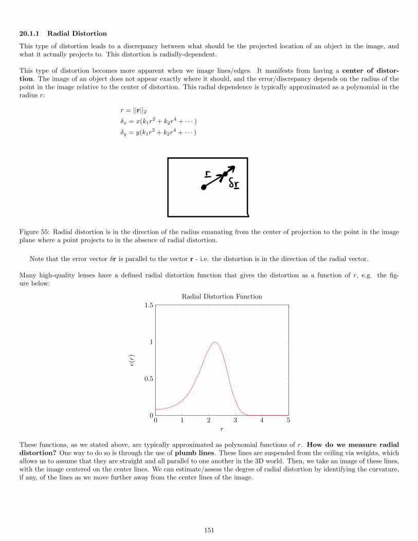
20.1.1 Radial Distortion

This type of distortion leads to a discrepancy between what should be the projected location of an object in the image, andwhat it actually projects to. This distortion is radially-dependent.

This type of distortion becomes more apparent when we image lines/edges. It manifests from having a center of distor-tion. The image of an object does not appear exactly where it should, and the error/discrepancy depends on the radius of thepoint in the image relative to the center of distortion. This radial dependence is typically approximated as a polynomial in theradius r:

r = ||r||2δx = x(k1r

2 + k2r4 + · · · )

δy = y(k1r2 + k2r

4 + · · · )

Figure 55: Radial distortion is in the direction of the radius emanating from the center of projection to the point in the imageplane where a point projects to in the absence of radial distortion.

Note that the error vector δr is parallel to the vector r - i.e. the distortion is in the direction of the radial vector.

Many high-quality lenses have a defined radial distortion function that gives the distortion as a function of r, e.g. the fig-ure below:

0 1 2 3 4 50

0.5

1

1.5

r

e(r)

Radial Distortion Function

These functions, as we stated above, are typically approximated as polynomial functions of r. How do we measure radialdistortion? One way to do so is through the use of plumb lines. These lines are suspended from the ceiling via weights, whichallows us to assume that they are straight and all parallel to one another in the 3D world. Then, we take an image of these lines,with the image centered on the center lines. We can estimate/assess the degree of radial distortion by identifying the curvature,if any, of the lines as we move further away from the center lines of the image.

151

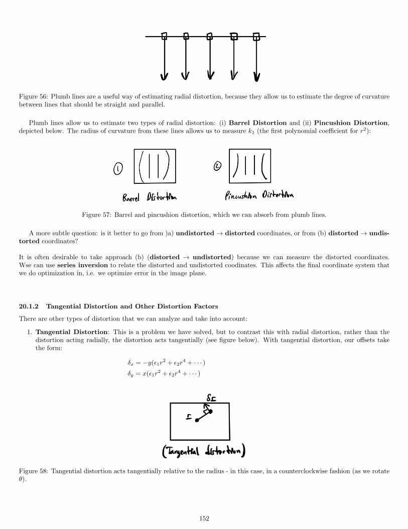
Figure 56: Plumb lines are a useful way of estimating radial distortion, because they allow us to estimate the degree of curvaturebetween lines that should be straight and parallel.

Plumb lines allow us to estimate two types of radial distortion: (i) Barrel Distortion and (ii) Pincushion Distortion,depicted below. The radius of curvature from these lines allows us to measure k1 (the first polynomial coefficient for r2):

Figure 57: Barrel and pincushion distortion, which we can absorb from plumb lines.

A more subtle question: is it better to go from )a) undistorted → distorted coordinates, or from (b) distorted → undis-torted coordinates?

It is often desirable to take approach (b) (distorted → undistorted) because we can measure the distorted coordinates.Wse can use series inversion to relate the distorted and undistorted coodinates. This affects the final coordinate system thatwe do optimization in, i.e. we optimize error in the image plane.

20.1.2 Tangential Distortion and Other Distortion Factors

There are other types of distortion that we can analyze and take into account:

1. Tangential Distortion: This is a problem we have solved, but to contrast this with radial distortion, rather than thedistortion acting radially, the distortion acts tangentially (see figure below). With tangential distortion, our offsets takethe form:

δx = −y(ε1r2 + ε2r

4 + · · · )δy = x(ε1r

2 + ε2r4 + · · · )

Figure 58: Tangential distortion acts tangentially relative to the radius - in this case, in a counterclockwise fashion (as we rotateθ).

152

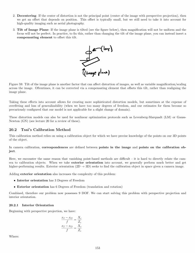
2. Decentering: If the center of distortion is not the principal point (center of the image with perspective projection), thenwe get an offset that depends on position. This offset is typically small, but we still need to take it into account forhigh-quality imaging such as aerial photography.

3. Tilt of Image Plane: If the image plane is tilted (see the figure below), then magnification will not be uniform and thefocus will not be perfect. In practice, to fix this, rather than changing the tilt of the image plane, you can instead insert acompensating element to offset this tilt.

Figure 59: Tilt of the image plane is another factor that can affect distortion of images, as well as variable magnification/scalingacross the image. Oftentimes, it can be corrected via a compensating element that offsets this tilt, rather than realigning theimage plane.

Taking these effects into account allows for creating more sophisticated distortion models, but sometimes at the expense ofoverfitting and loss of generalizability (when we have too many degrees of freedom, and our estimates for them become soprecariously configured that our model is not applicable for a slight change of domain).

These distortion models can also be used for nonlinear optimization protocols such as Levenberg-Marquadt (LM) or Gauss-Newton (GN) (see lecture 20 for a review of these).

20.2 Tsai’s Calibration Method

This calibration method relies on using a calibration object for which we have precise knowledge of the points on our 3D pointsof the object.

In camera calibration, correspondences are defined between points in the image and points on the calibration ob-ject.

Here, we encounter the same reason that vanishing point-based methods are difficult - it is hard to directly relate the cam-era to calibration objects. When we take exterior orientation into account, we generally perform much better and gethigher-performing results. Exterior orientation (2D → 3D) seeks to find the calibration object in space given a camera image.

Adding exterior orientation also increases the complexity of this problem:

• Interior orientation has 3 Degrees of Freedom

• Exterior orientation has 6 Degrees of Freedom (translation and rotation)

Combined, therefore our problem now possesses 9 DOF. We can start solving this problem with perspective projection andinterior orientation.

20.2.1 Interior Orientation

Beginning with perspective projection, we have:

xI − xOf

=Xc

ZcxI − xO

f=Xc

Zc

Where:

153

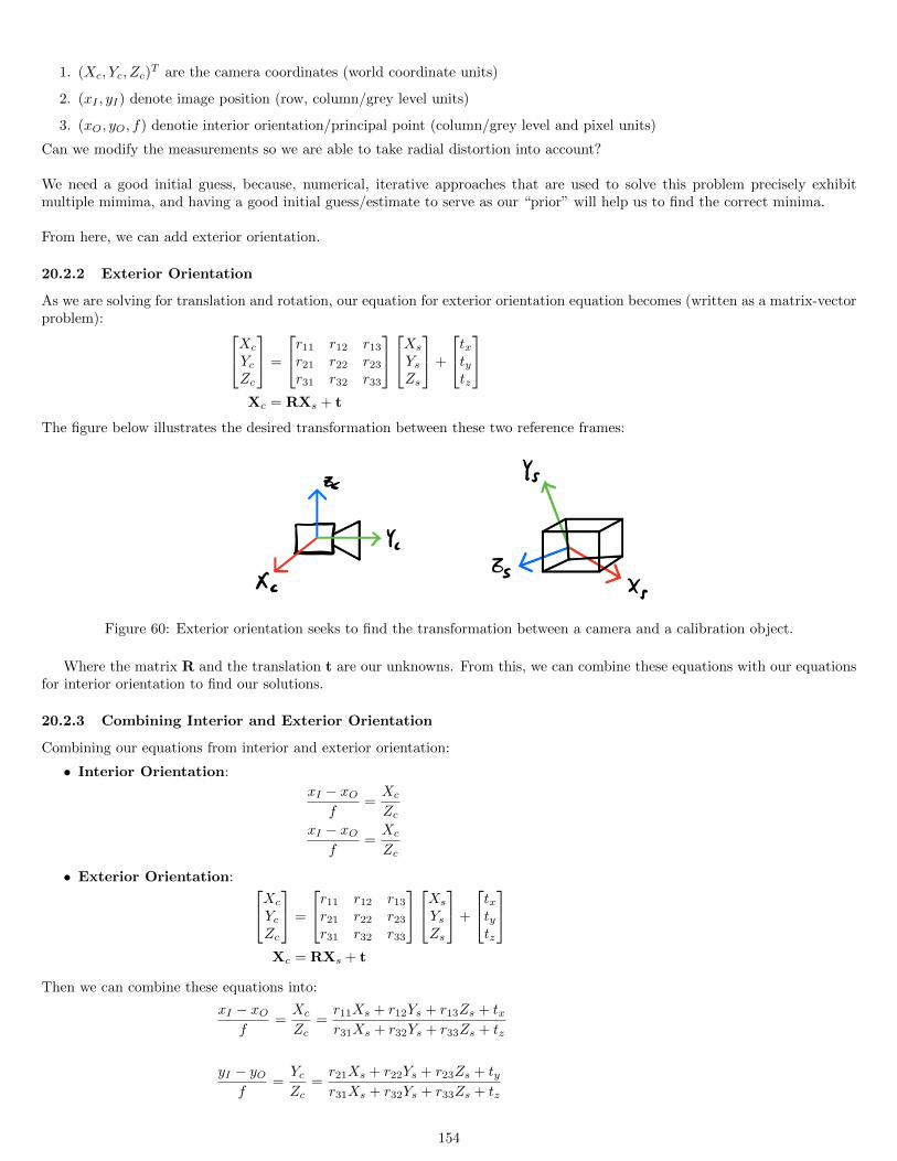
1. (Xc, Yc, Zc)T are the camera coordinates (world coordinate units)

2. (xI , yI) denote image position (row, column/grey level units)

3. (xO, yO, f) denotie interior orientation/principal point (column/grey level and pixel units)

Can we modify the measurements so we are able to take radial distortion into account?

We need a good initial guess, because, numerical, iterative approaches that are used to solve this problem precisely exhibitmultiple mimima, and having a good initial guess/estimate to serve as our “prior” will help us to find the correct minima.

From here, we can add exterior orientation.

20.2.2 Exterior Orientation

As we are solving for translation and rotation, our equation for exterior orientation equation becomes (written as a matrix-vectorproblem): Xc

YcZc

=

r11 r12 r13

r21 r22 r23

r31 r32 r33

Xs

YsZs

+

txtytz

Xc = RXs + t

The figure below illustrates the desired transformation between these two reference frames:

Figure 60: Exterior orientation seeks to find the transformation between a camera and a calibration object.

Where the matrix R and the translation t are our unknowns. From this, we can combine these equations with our equationsfor interior orientation to find our solutions.

20.2.3 Combining Interior and Exterior Orientation

Combining our equations from interior and exterior orientation:

• Interior Orientation:

xI − xOf

=Xc

ZcxI − xO

f=Xc

Zc

• Exterior Orientation: Xc

YcZc

=

r11 r12 r13

r21 r22 r23

r31 r32 r33

Xs

YsZs

+

txtytz

Xc = RXs + t

Then we can combine these equations into:

xI − xOf

=Xc

Zc=r11Xs + r12Ys + r13Zs + txr31Xs + r32Ys + r33Zs + tz

yI − yOf

=YcZc

=r21Xs + r22Ys + r23Zs + tyr31Xs + r32Ys + r33Zs + tz

154

Written this way, we can map directly from image coordinates to calibration objects.

How can we find f and tz, as well as mitigate radial distortion?

Let’s start by looking at this problem in polar coordinates. Radial distortion only changes radial lengths (r), and not an-gle (θ). Changing f or Zc changes only radius/magnification. Let’s use this factor to “forget” about the angle.

We can also remove additional DOF by dividing our combined equations by one another:

xI − xOyI − y0

=r11Xs+r12Ys+r13Zs+txr31Xs+r32Ys+r33Zs+tzr21Xs+r22Ys+r23Zs+tyr31Xs+r32Ys+r33Zs+tz

=r11Xs + r12Ys + r13Zs + txr21Xs + r22Ys + r23Zs + ty

We can see that combining these constraints removes our DOF tz, giving us 8 constraints rather than 9. Cross-multiplying andterm consolidation gives:

(XSy′I)r11 + (YSy

′I)r12 + (ZSy

′I)r13 + y′Itx − (XSx

′I)r21 − (YSx

′I)r22 − (ZSx

′I)r23 − x′Ity = 0

A few notes on this consolidated homogeneous equation:

• Since our unknowns are the rij values, we have a linear combination/equation of our unknowns! The coefficients they aremultiplied by are either our observed image positions or the positions of the correspondences/keypoints on the calibrationobject.

• Note that we subtract out an estimate of the center of projection. The estimation error of this center of projection affectsadjacent points the most, as a slight miscalculation can greatly affect the calculations above - and as a result we throw outall correspondences that are ε-close (for some ε > 0 to the center of the image.

• Each correspondence between image coordinates and the points on the calibration object gives one of these equations:“This point in the image corresponds to another point on the calibration object”.

As we have asked for the other frameworks and systems we have analyzed: How many correspondences do we need? Let’sconsider which unknowns appear in the equations, and which do not:

• DOF/unknowns in the equations: r11, r12, r13, r21, r22, r23, tx, ty (8 unknowns)

• DOF/unknowns not in the equations: r31, r32, r33, tz, f (5 unknowns)

Can this inform of how we can solve this problem? Let’s consider the following points:

• We are not yet enforcing orthonormality of the rotation matrices, i.e. RTR = I.

• We can solve for the last row of the rotation matrix containing the unknowns r31, r32, r33 through finding the cross productof the first two rows of this matrix.

• Having 8 unknowns suggests that we need at least 8 correspondences, but because this equation is homogeneous, thereis scale factor ambiguity (i.e. doubling all the variables does not change the righthand side value of the equation).The solution to account for this scale factor ambiguity is to set/fix one of these variables to a constant value. Fixing anunknown means we now have 7 DOF (rather than 8), and therefore, we actually need 7 correspondences. Solvingwith 7 (or more) correspondences gives us a multiple of the solution. Solving with exactly 7 correspondences gives us 7equations and 7 unknowns, which we can solve with, for instance, Gauss-Jordan elimination. More correspondences aredesirable because they allow us to estimate both solutions and the error associated with these solutions.

• These solutions give us values for the 8 unknowns in the equation above: r′11, r′12, r

′13, r

′21, r

′22, r

′23, tx, ty = 1 (where ty is the

fixed parameter to account for scale ambiguity). However, as aforementioned these values are scaled versions of the truesolution, and we can compute this scale factor by noting that because the rows of our (soon to be) orthonormal rotationmatrix must have unit length - therefore the scale factor is given by computing the length of the rows of this matrix:

s =1√

r′112 + r′12

2 + r′132

OR

s =1√

r′212 + r′22

2 + r′232

155

A good sanity check: these two variables should evaluate to approximately the same value - if they do not, this is oftenone indicator of correspondence mismatch.

With this scale factor computed we can find the true values of our solution by multiplying the scaled solutions with this scalefactor:

s(r′11, r′12, r

′13, r

′21, r

′22, r

′23, tx, ty = 1)→ r11, r12, r13, r21, r22, r23, tx, ty

Note that we also have not (yet) enforced orthonormality of the first two rows in the rotation matrix, i.e. our goal is to have (orminimize):

r′11r′21 + r′12r

′22 + r′13r

′23 = 0

To accomplish this, we will use the idea of “squaring up”.

20.2.4 “Squaring Up”

Squaring up is one method for ensuring that vectors are numerically/approximately orthogonal to one another. This techniqueanswers the question of “Given a set of orthogonal vectors, what is the nearest set of orthogonal vectors?”

The figure below highlights that given vectors a and b, we can find the nearest set of rotated vectors a′ and b′ using thefollowing, which states that adjustments to each vector in the pair are made in the direction of the other vector:

a′ = a + kb

b′ = b + ka

Since we want this dot product to be zero, we can solve for the scale k by taking the dot product of a′ and b′ and setting itequal to zero:

a′ · b′ = (a + kb)(b + ka) = 0

= a · b + (a · a + b · b)k + k2 + a · b = 0

This equation produces a quadratic equation in k, but unfortunately, as we approach our solution point, this sets the secondand third terms, which k depends on, to values near zero, creating numerical instability and consequently making this a poorapproach for solving for k. A better approach is to use the approximation:

k ≈ −(

a · b2

)It is much easier to solve for this and iterate over it a couple of times. I.e. instead of using the approach above, we use:

x =2c

−b±√b2 − 4ac

Where we note that the “standard” quadratic solution is given by:

x =−b±

√b2 − 4ac

2a

It is important to consider both of these approaches because of floating-point precision accuracy - in any case, as we approachthe solution point, one of the two forms of these solutions will not perform well, and the other form will perform substantiallybetter.

With this, we are able to iteratively solve for k until our two vectors have a dot product approximately equal to zero. Oncethis dot product is approximately zero, we are done! We have enforced orthonormality of the first two rows of the rotationmatrix, which allows us to find an orthonormal third row of the rotation matrix by taking a cross product of the first two rows.Therefore, we then have an orthonormal rotation matrix.

20.2.5 Planar Target

Planar target is an example calibration object that possesses desirable properties, namely, as we will see below, that it reducesthe number of correspondences we need from 7 to 5. Additionally, planar targets are generally easy to make, store, and allow

156

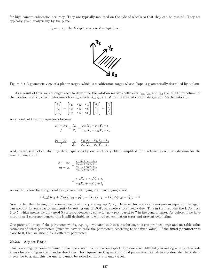
for high camera calibration accuracy. They are typically mounted on the side of wheels so that they can be rotated. They aretypically given analytically by the plane:

Zs = 0, i.e. the XY-plane where Z is equal to 0.

Figure 61: A geometric view of a planar target, which is a calibration target whose shape is geometrically described by a plane.

As a result of this, we no longer need to determine the rotation matrix coefficients r13, r23, and r33 (i.e. the third column ofthe rotation matrix, which determines how Zs affects Xc, Yc, and Zc in the rotated coordinate system. Mathematically:Xc

YcZc

=

r11 r12 r13

r21 r22 r23

r31 r32 r33

Xs

Ys0

+

txtytz

As a result of this, our equations become:

xI − xOf

=Xc

Zc=r11Xs + r12Ys + txr31Xs + r32Ys + tz

yI − yOf

=YcZc

=r21Xs + r22Ys + tyr31Xs + r32Ys + tz

And, as we saw before, dividing these equations by one another yields a simplified form relative to our last division for thegeneral case above:

xI − xOyI − y0

=r11Xs+r12Ys+txr31Xs+r32Ys+tzr21Xs+r22Ys+tyr31Xs+r32Ys+tz

=r11Xs + r12Ys + txr21Xs + r22Ys + ty

As we did before for the general case, cross-multiplying and rearranging gives:

(XSy′I)r11 + (YSy

′I)r12 + y′Itx − (XSx

′I)r21 − (YSx

′I)r22 − x′Ity = 0

Now, rather than having 8 unknowns, we have 6: r11, r12, r21, r22, tx, ty. Because this is also a homogeneous equation, we againcan account for scale factor ambiguity by setting one of DOF/parameters to a fixed value. This in turn reduces the DOF from6 to 5, which means we only need 5 correspondences to solve for now (compared to 7 in the general case). As before, if we havemore than 5 correspondences, this is still desirable as it will reduce estimation error and prevent overfitting.

One potential issue: if the parameter we fix, e.g. ty, evaluates to 0 in our solution, this can produce large and unstable valueestimates of other parameters (since we have to scale the parameters according to the fixed value). If the fixed parameter isclose to 0, then we should fix a different parameter.

20.2.6 Aspect Ratio

This is no longer a common issue in machine vision now, but when aspect ratios were set differently in analog with photo-diodearrays for stepping in the x and y directions, this required setting an additional parameter to analytically describe the scale ofx relative to y, and this parameter cannot be solved without a planar target.

157

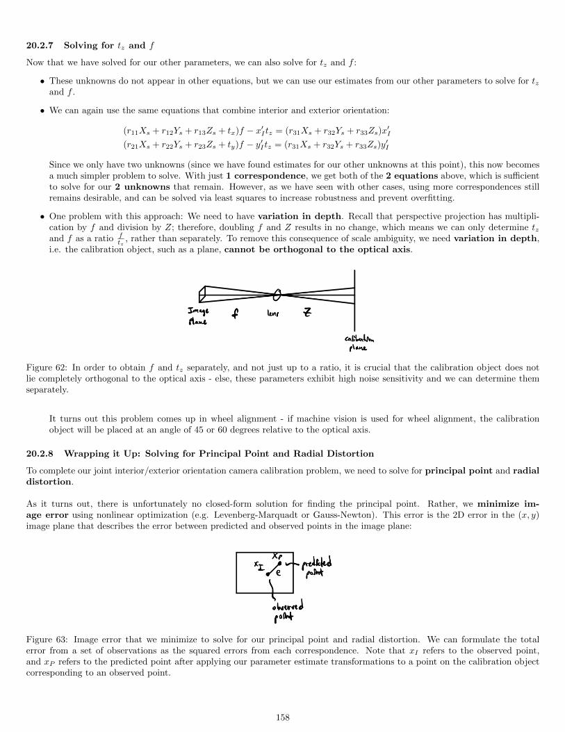
20.2.7 Solving for tz and f

Now that we have solved for our other parameters, we can also solve for tz and f :

• These unknowns do not appear in other equations, but we can use our estimates from our other parameters to solve for tzand f .

• We can again use the same equations that combine interior and exterior orientation:

(r11Xs + r12Ys + r13Zs + tx)f − x′Itz = (r31Xs + r32Ys + r33Zs)x′I

(r21Xs + r22Ys + r23Zs + ty)f − y′Itz = (r31Xs + r32Ys + r33Zs)y′I

Since we only have two unknowns (since we have found estimates for our other unknowns at this point), this now becomesa much simpler problem to solve. With just 1 correspondence, we get both of the 2 equations above, which is sufficientto solve for our 2 unknowns that remain. However, as we have seen with other cases, using more correspondences stillremains desirable, and can be solved via least squares to increase robustness and prevent overfitting.

• One problem with this approach: We need to have variation in depth. Recall that perspective projection has multipli-cation by f and division by Z; therefore, doubling f and Z results in no change, which means we can only determine tzand f as a ratio f

tz, rather than separately. To remove this consequence of scale ambiguity, we need variation in depth,

i.e. the calibration object, such as a plane, cannot be orthogonal to the optical axis.

Figure 62: In order to obtain f and tz separately, and not just up to a ratio, it is crucial that the calibration object does notlie completely orthogonal to the optical axis - else, these parameters exhibit high noise sensitivity and we can determine themseparately.

It turns out this problem comes up in wheel alignment - if machine vision is used for wheel alignment, the calibrationobject will be placed at an angle of 45 or 60 degrees relative to the optical axis.

20.2.8 Wrapping it Up: Solving for Principal Point and Radial Distortion

To complete our joint interior/exterior orientation camera calibration problem, we need to solve for principal point and radialdistortion.

As it turns out, there is unfortunately no closed-form solution for finding the principal point. Rather, we minimize im-age error using nonlinear optimization (e.g. Levenberg-Marquadt or Gauss-Newton). This error is the 2D error in the (x, y)image plane that describes the error between predicted and observed points in the image plane:

Figure 63: Image error that we minimize to solve for our principal point and radial distortion. We can formulate the totalerror from a set of observations as the squared errors from each correspondence. Note that xI refers to the observed point,and xP refers to the predicted point after applying our parameter estimate transformations to a point on the calibration objectcorresponding to an observed point.

158

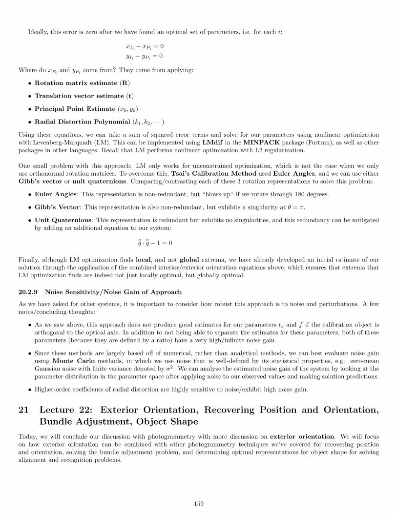
Ideally, this error is zero after we have found an optimal set of parameters, i.e. for each i:

xIi − xPi = 0

yIi − yPi = 0

Where do xPi and yPi come from? They come from applying:

• Rotation matrix estimate (R)

• Translation vector estimate (t)

• Principal Point Estimate (x0, y0)

• Radial Distortion Polynomial (k1, k2, · · · )

Using these equations, we can take a sum of squared error terms and solve for our parameters using nonlinear optimizationwith Levenberg-Marquadt (LM). This can be implemented using LMdif in the MINPACK package (Fortran), as well as otherpackages in other languages. Recall that LM performs nonlinear optimization with L2 regularization.

One small problem with this approach: LM only works for unconstrained optimization, which is not the case when we onlyuse orthonormal rotation matrices. To overcome this, Tsai’s Calibration Method used Euler Angles, and we can use eitherGibb’s vector or unit quaternions. Comparing/contrasting each of these 3 rotation representations to solve this problem:

• Euler Angles: This representation is non-redundant, but “blows up” if we rotate through 180 degrees.

• Gibb’s Vector: This representation is also non-redundant, but exhibits a singularity at θ = π.

• Unit Quaternions: This representation is redundant but exhibits no singularities, and this redundancy can be mitigatedby adding an additional equation to our system:

oq · oq − 1 = 0

Finally, although LM optimization finds local, and not global extrema, we have already developed an initial estimate of oursolution through the application of the combined interior/exterior orientation equations above, which ensures that extrema thatLM optimization finds are indeed not just locally optimal, but globally optimal.

20.2.9 Noise Sensitivity/Noise Gain of Approach

As we have asked for other systems, it is important to consider how robust this approach is to noise and perturbations. A fewnotes/concluding thoughts:

• As we saw above, this approach does not produce good estimates for our parameters tz and f if the calibration object isorthogonal to the optical axis. In addition to not being able to separate the estimates for these parameters, both of theseparameters (because they are defined by a ratio) have a very high/infinite noise gain.

• Since these methods are largely based off of numerical, rather than analytical methods, we can best evaluate noise gainusing Monte Carlo methods, in which we use noise that is well-defined by its statistical properties, e.g. zero-meanGaussian noise with finite variance denoted by σ2. We can analyze the estimated noise gain of the system by looking at theparameter distribution in the parameter space after applying noise to our observed values and making solution predictions.

• Higher-order coefficients of radial distortion are highly sensitive to noise/exhibit high noise gain.

21 Lecture 22: Exterior Orientation, Recovering Position and Orientation,Bundle Adjustment, Object Shape

Today, we will conclude our discussion with photogrammetry with more discussion on exterior orientation. We will focuson how exterior orientation can be combined with other photogrammetry techniques we’ve covered for recovering positionand orientation, solving the bundle adjustment problem, and determining optimal representations for object shape for solvingalignment and recognition problems.

159

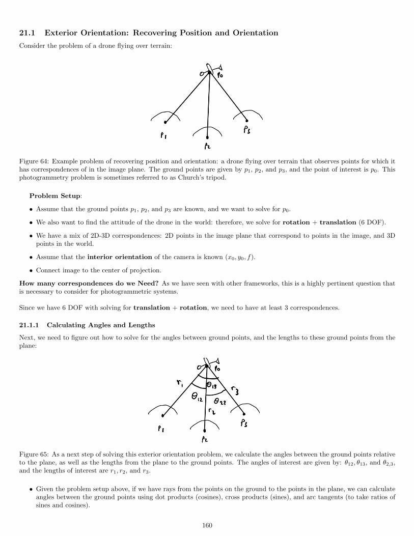
21.1 Exterior Orientation: Recovering Position and Orientation

Consider the problem of a drone flying over terrain:

Figure 64: Example problem of recovering position and orientation: a drone flying over terrain that observes points for which ithas correspondences of in the image plane. The ground points are given by p1, p2, and p3, and the point of interest is p0. Thisphotogrammetry problem is sometimes referred to as Church’s tripod.

Problem Setup:

• Assume that the ground points p1, p2, and p3 are known, and we want to solve for p0.

• We also want to find the attitude of the drone in the world: therefore, we solve for rotation + translation (6 DOF).

• We have a mix of 2D-3D correspondences: 2D points in the image plane that correspond to points in the image, and 3Dpoints in the world.

• Assume that the interior orientation of the camera is known (x0, y0, f).

• Connect image to the center of projection.

How many correspondences do we Need? As we have seen with other frameworks, this is a highly pertinent question thatis necessary to consider for photogrammetric systems.

Since we have 6 DOF with solving for translation + rotation, we need to have at least 3 correspondences.

21.1.1 Calculating Angles and Lengths

Next, we need to figure out how to solve for the angles between ground points, and the lengths to these ground points from theplane:

Figure 65: As a next step of solving this exterior orientation problem, we calculate the angles between the ground points relativeto the plane, as well as the lengths from the plane to the ground points. The angles of interest are given by: θ12, θ13, and θ2,3,and the lengths of interest are r1, r2, and r3.

• Given the problem setup above, if we have rays from the points on the ground to the points in the plane, we can calculateangles between the ground points using dot products (cosines), cross products (sines), and arc tangents (to take ratios ofsines and cosines).

160

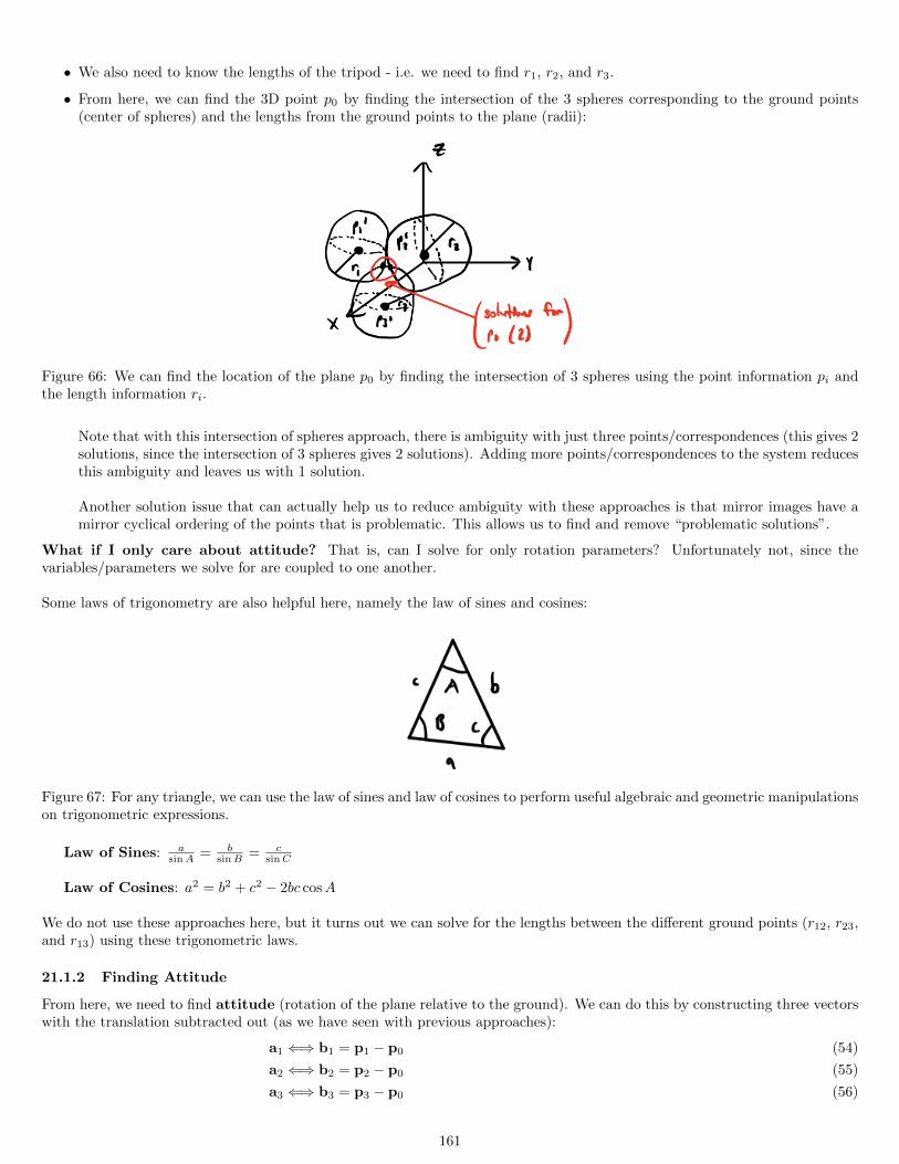
• We also need to know the lengths of the tripod - i.e. we need to find r1, r2, and r3.

• From here, we can find the 3D point p0 by finding the intersection of the 3 spheres corresponding to the ground points(center of spheres) and the lengths from the ground points to the plane (radii):

Figure 66: We can find the location of the plane p0 by finding the intersection of 3 spheres using the point information pi andthe length information ri.

Note that with this intersection of spheres approach, there is ambiguity with just three points/correspondences (this gives 2solutions, since the intersection of 3 spheres gives 2 solutions). Adding more points/correspondences to the system reducesthis ambiguity and leaves us with 1 solution.

Another solution issue that can actually help us to reduce ambiguity with these approaches is that mirror images have amirror cyclical ordering of the points that is problematic. This allows us to find and remove “problematic solutions”.

What if I only care about attitude? That is, can I solve for only rotation parameters? Unfortunately not, since thevariables/parameters we solve for are coupled to one another.

Some laws of trigonometry are also helpful here, namely the law of sines and cosines:

Figure 67: For any triangle, we can use the law of sines and law of cosines to perform useful algebraic and geometric manipulationson trigonometric expressions.

Law of Sines: asinA = b

sinB = csinC

Law of Cosines: a2 = b2 + c2 − 2bc cosA

We do not use these approaches here, but it turns out we can solve for the lengths between the different ground points (r12, r23,and r13) using these trigonometric laws.

21.1.2 Finding Attitude

From here, we need to find attitude (rotation of the plane relative to the ground). We can do this by constructing three vectorswith the translation subtracted out (as we have seen with previous approaches):

a1 ⇐⇒ b1 = p1 − p0 (54)

a2 ⇐⇒ b2 = p2 − p0 (55)

a3 ⇐⇒ b3 = p3 − p0 (56)

161

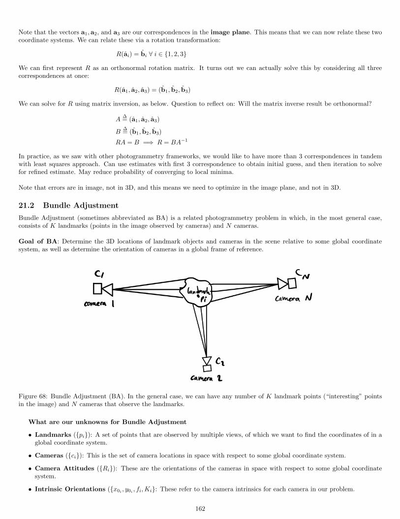
Note that the vectors a1,a2, and a3 are our correspondences in the image plane. This means that we can now relate these twocoordinate systems. We can relate these via a rotation transformation:

R(ai) = bi ∀ i ∈ 1, 2, 3

We can first represent R as an orthonormal rotation matrix. It turns out we can actually solve this by considering all threecorrespondences at once:

R(a1, a2, a3) = (b1, b2, b3)

We can solve for R using matrix inversion, as below. Question to reflect on: Will the matrix inverse result be orthonormal?

A∆= (a1, a2, a3)

B∆= (b1, b2, b3)

RA = B =⇒ R = BA−1

In practice, as we saw with other photogrammetry frameworks, we would like to have more than 3 correspondences in tandemwith least squares approach. Can use estimates with first 3 correspondence to obtain initial guess, and then iteration to solvefor refined estimate. May reduce probability of converging to local minima.

Note that errors are in image, not in 3D, and this means we need to optimize in the image plane, and not in 3D.

21.2 Bundle Adjustment

Bundle Adjustment (sometimes abbreviated as BA) is a related photogrammetry problem in which, in the most general case,consists of K landmarks (points in the image observed by cameras) and N cameras.

Goal of BA: Determine the 3D locations of landmark objects and cameras in the scene relative to some global coordinatesystem, as well as determine the orientation of cameras in a global frame of reference.

Figure 68: Bundle Adjustment (BA). In the general case, we can have any number of K landmark points (“interesting” pointsin the image) and N cameras that observe the landmarks.

What are our unknowns for Bundle Adjustment

• Landmarks (pi): A set of points that are observed by multiple views, of which we want to find the coordinates of in aglobal coordinate system.

• Cameras (ci): This is the set of camera locations in space with respect to some global coordinate system.

• Camera Attitudes (Ri): These are the orientations of the cameras in space with respect to some global coordinatesystem.

• Intrinsic Orientations (x0i , y0i , fi,Ki: These refer to the camera intrinsics for each camera in our problem.

162

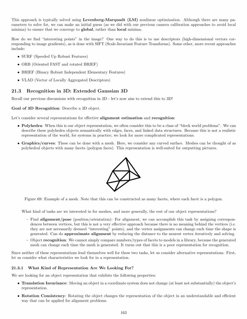
This approach is typically solved using Levenberg-Marquadt (LM) nonlinear optimization. Although there are many pa-rameters to solve for, we can make an initial guess (as we did with our previous camera calibration approaches to avoid localminima) to ensure that we converge to global, rather than local minima.

How do we find “interesting points” in the image? One way to do this is to use descriptors (high-dimensional vectors cor-responding to image gradients), as is done with SIFT (Scale-Invariant Feature Transforms). Some other, more recent approachesinclude:

• SURF (Speeded Up Robust Features)

• ORB (Oriented FAST and rotated BRIEF)

• BRIEF (Binary Robust Independent Elementary Features)

• VLAD (Vector of Locally Aggregated Descriptors)

21.3 Recognition in 3D: Extended Gaussian 3D

Recall our previous discussions with recognition in 2D - let’s now aim to extend this to 3D!

Goal of 3D Recognition: Describe a 3D object.

Let’s consider several representations for effective alignment estimation and recognition:

• Polyhedra: When this is our object representation, we often consider this to be a class of “block world problems”. We candescribe these polyhedra objects semantically with edges, faces, and linked data structures. Because this is not a realisticrepresentation of the world, for systems in practice, we look for more complicated representations.

• Graphics/curves: These can be done with a mesh. Here, we consider any curved surface. Meshes can be thought of aspolyhedral objects with many facets (polygon faces). This representation is well-suited for outputting pictures.

Figure 69: Example of a mesh. Note that this can be constructed as many facets, where each facet is a polygon.

What kind of tasks are we interested in for meshes, and more generally, the rest of our object representations?

– Find alignment/pose (position/orientation): For alignment, we can accomplish this task by assigning correspon-dences between vertices, but this is not a very effective approach because there is no meaning behind the vertices (i.e.they are not necessarily deemed “interesting” points), and the vertex assignments can change each time the shape isgenerated. Can do approximate alignment by reducing the distance to the nearest vertex iteratively and solving.

– Object recognition: We cannot simply compare numbers/types of facets to models in a library, because the generatedmesh can change each time the mesh is generated. It turns out that this is a poor representation for recognition.

Since neither of these representations lend themselves well for these two tasks, let us consider alternative representations. First,let us consider what characteristics we look for in a representation.

21.3.1 What Kind of Representation Are We Looking For?

We are looking for an object representation that exhibits the following properties:

• Translation Invariance: Moving an object in a coordinate system does not change (at least not substantially) the object’srepresentation.

• Rotation Consistency: Rotating the object changes the representation of the object in an understandable and efficientway that can be applied for alignment problems.

163

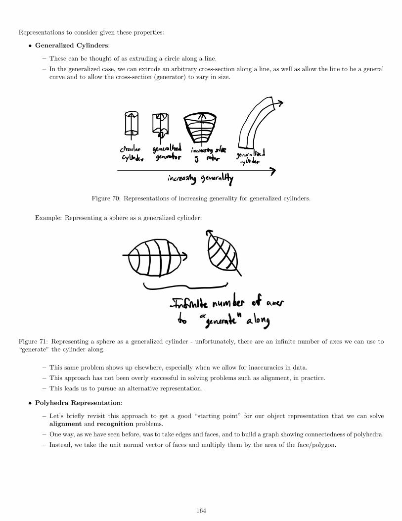
Representations to consider given these properties:

• Generalized Cylinders:

– These can be thought of as extruding a circle along a line.

– In the generalized case, we can extrude an arbitrary cross-section along a line, as well as allow the line to be a generalcurve and to allow the cross-section (generator) to vary in size.

Figure 70: Representations of increasing generality for generalized cylinders.

Example: Representing a sphere as a generalized cylinder:

Figure 71: Representing a sphere as a generalized cylinder - unfortunately, there are an infinite number of axes we can use to“generate” the cylinder along.

– This same problem shows up elsewhere, especially when we allow for inaccuracies in data.

– This approach has not been overly successful in solving problems such as alignment, in practice.

– This leads us to pursue an alternative representation.

• Polyhedra Representation:

– Let’s briefly revisit this approach to get a good “starting point” for our object representation that we can solvealignment and recognition problems.

– One way, as we have seen before, was to take edges and faces, and to build a graph showing connectedness of polyhedra.

– Instead, we take the unit normal vector of faces and multiply them by the area of the face/polygon.

164

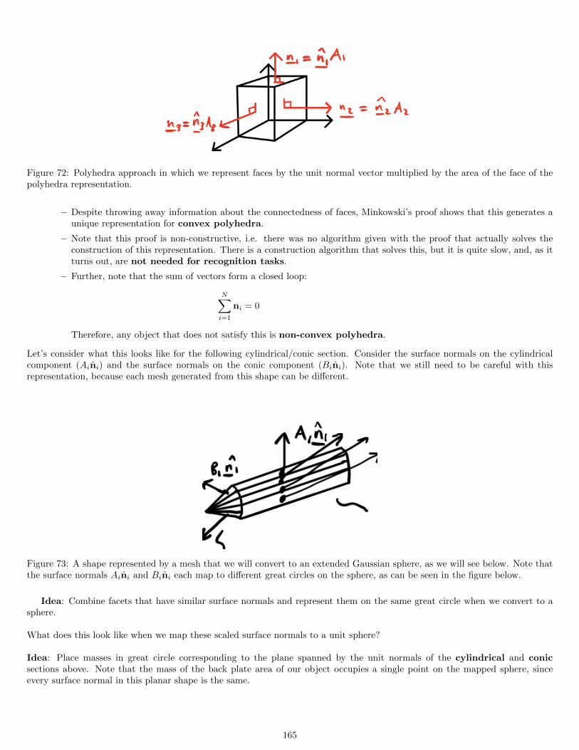
Figure 72: Polyhedra approach in which we represent faces by the unit normal vector multiplied by the area of the face of thepolyhedra representation.

– Despite throwing away information about the connectedness of faces, Minkowski’s proof shows that this generates aunique representation for convex polyhedra.

– Note that this proof is non-constructive, i.e. there was no algorithm given with the proof that actually solves theconstruction of this representation. There is a construction algorithm that solves this, but it is quite slow, and, as itturns out, are not needed for recognition tasks.

– Further, note that the sum of vectors form a closed loop:

N∑i=1

ni = 0

Therefore, any object that does not satisfy this is non-convex polyhedra.

Let’s consider what this looks like for the following cylindrical/conic section. Consider the surface normals on the cylindricalcomponent (Aini) and the surface normals on the conic component (Bini). Note that we still need to be careful with thisrepresentation, because each mesh generated from this shape can be different.

Figure 73: A shape represented by a mesh that we will convert to an extended Gaussian sphere, as we will see below. Note thatthe surface normals Aini and Bini each map to different great circles on the sphere, as can be seen in the figure below.

Idea: Combine facets that have similar surface normals and represent them on the same great circle when we convert to asphere.

What does this look like when we map these scaled surface normals to a unit sphere?

Idea: Place masses in great circle corresponding to the plane spanned by the unit normals of the cylindrical and conicsections above. Note that the mass of the back plate area of our object occupies a single point on the mapped sphere, sinceevery surface normal in this planar shape is the same.

165

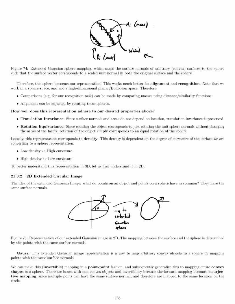
Figure 74: Extended Gaussian sphere mapping, which maps the surface normals of arbitrary (convex) surfaces to the spheresuch that the surface vector corresponds to a scaled unit normal in both the original surface and the sphere.

Therefore, this sphere becoems our representation! This works much better for alignment and recognition. Note that wework in a sphere space, and not a high-dimensional planar/Euclidean space. Therefore:

• Comparisons (e.g. for our recognition task) can be made by comparing masses using distance/similarity functions.

• Alignment can be adjusted by rotating these spheres.

How well does this representation adhere to our desired properties above?

• Translation Invariance: Since surface normals and areas do not depend on location, translation invariance is preserved.

• Rotation Equivariance: Since rotating the object corresponds to just rotating the unit sphere normals without changingthe areas of the facets, rotation of the object simply corresponds to an equal rotation of the sphere.

Loosely, this representation corresponds to density. This density is dependent on the degree of curvature of the surface we areconverting to a sphere representation:

• Low density ↔ High curvature

• High density ↔ Low curvature

To better understand this representation in 3D, let us first understand it in 2D.

21.3.2 2D Extended Circular Image

The idea of the extended Gaussian Image: what do points on an object and points on a sphere have in common? They have thesame surface normals.

Figure 75: Representation of our extended Gaussian image in 2D. The mapping between the surface and the sphere is determinedby the points with the same surface normals.

Gauss: This extended Gaussian image representation is a way to map arbitrary convex objects to a sphere by mappingpoints with the same surface normals.

We can make this (invertible) mapping in a point-point fashion, and subsequently generalize this to mapping entire convexshapes to a sphere. There are issues with non-convex objects and invertibility because the forward mapping becomes a surjec-tive mapping, since multiple ponts can have the same surface normal, and therefore are mapped to the same location on thecircle.

166

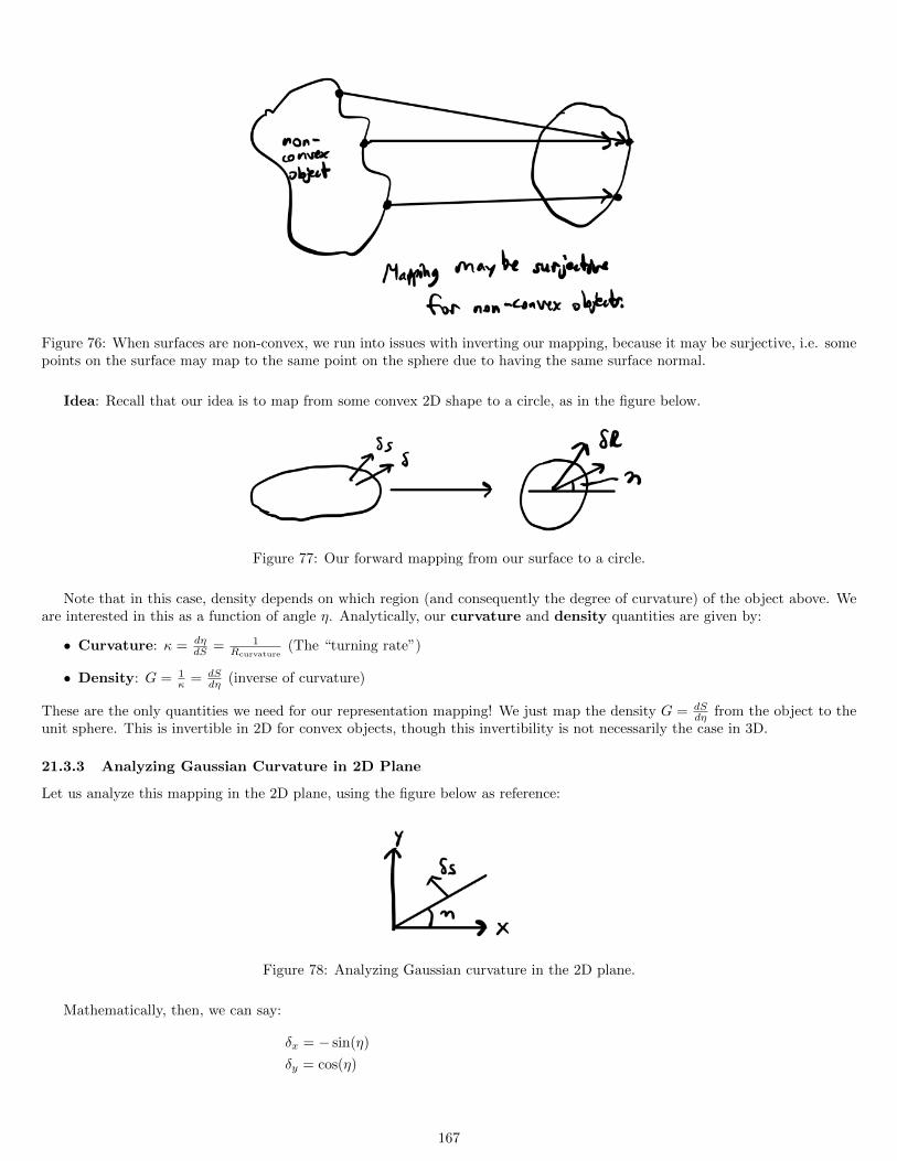
Figure 76: When surfaces are non-convex, we run into issues with inverting our mapping, because it may be surjective, i.e. somepoints on the surface may map to the same point on the sphere due to having the same surface normal.

Idea: Recall that our idea is to map from some convex 2D shape to a circle, as in the figure below.

Figure 77: Our forward mapping from our surface to a circle.

Note that in this case, density depends on which region (and consequently the degree of curvature) of the object above. Weare interested in this as a function of angle η. Analytically, our curvature and density quantities are given by:

• Curvature: κ = dηdS = 1

Rcurvature(The “turning rate”)

• Density: G = 1κ = dS

dη (inverse of curvature)

These are the only quantities we need for our representation mapping! We just map the density G = dSdη from the object to the

unit sphere. This is invertible in 2D for convex objects, though this invertibility is not necessarily the case in 3D.

21.3.3 Analyzing Gaussian Curvature in 2D Plane

Let us analyze this mapping in the 2D plane, using the figure below as reference:

Figure 78: Analyzing Gaussian curvature in the 2D plane.

Mathematically, then, we can say:

δx = − sin(η)

δy = cos(η)

167

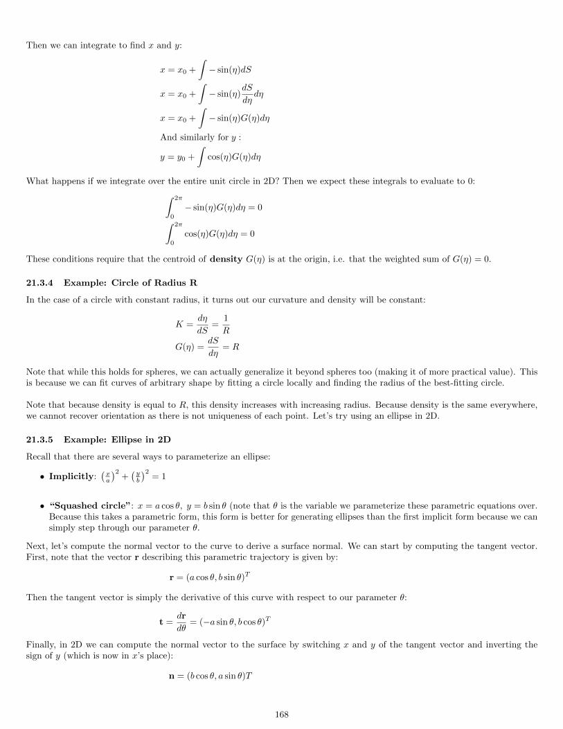
Then we can integrate to find x and y:

x = x0 +

∫− sin(η)dS

x = x0 +

∫− sin(η)

dS

dηdη

x = x0 +

∫− sin(η)G(η)dη

And similarly for y :

y = y0 +

∫cos(η)G(η)dη

What happens if we integrate over the entire unit circle in 2D? Then we expect these integrals to evaluate to 0:∫ 2π

0

− sin(η)G(η)dη = 0∫ 2π

0

cos(η)G(η)dη = 0

These conditions require that the centroid of density G(η) is at the origin, i.e. that the weighted sum of G(η) = 0.

21.3.4 Example: Circle of Radius R

In the case of a circle with constant radius, it turns out our curvature and density will be constant:

K =dη

dS=

1

R

G(η) =dS

dη= R

Note that while this holds for spheres, we can actually generalize it beyond spheres too (making it of more practical value). Thisis because we can fit curves of arbitrary shape by fitting a circle locally and finding the radius of the best-fitting circle.

Note that because density is equal to R, this density increases with increasing radius. Because density is the same everywhere,we cannot recover orientation as there is not uniqueness of each point. Let’s try using an ellipse in 2D.

21.3.5 Example: Ellipse in 2D

Recall that there are several ways to parameterize an ellipse:

• Implicitly:(xa

)2+(yb

)2= 1

• “Squashed circle”: x = a cos θ, y = b sin θ (note that θ is the variable we parameterize these parametric equations over.Because this takes a parametric form, this form is better for generating ellipses than the first implicit form because we cansimply step through our parameter θ.

Next, let’s compute the normal vector to the curve to derive a surface normal. We can start by computing the tangent vector.First, note that the vector r describing this parametric trajectory is given by:

r = (a cos θ, b sin θ)T

Then the tangent vector is simply the derivative of this curve with respect to our parameter θ:

t =dr

dθ= (−a sin θ, b cos θ)T

Finally, in 2D we can compute the normal vector to the surface by switching x and y of the tangent vector and inverting thesign of y (which is now in x’s place):

n = (b cos θ, a sin θ)T

168

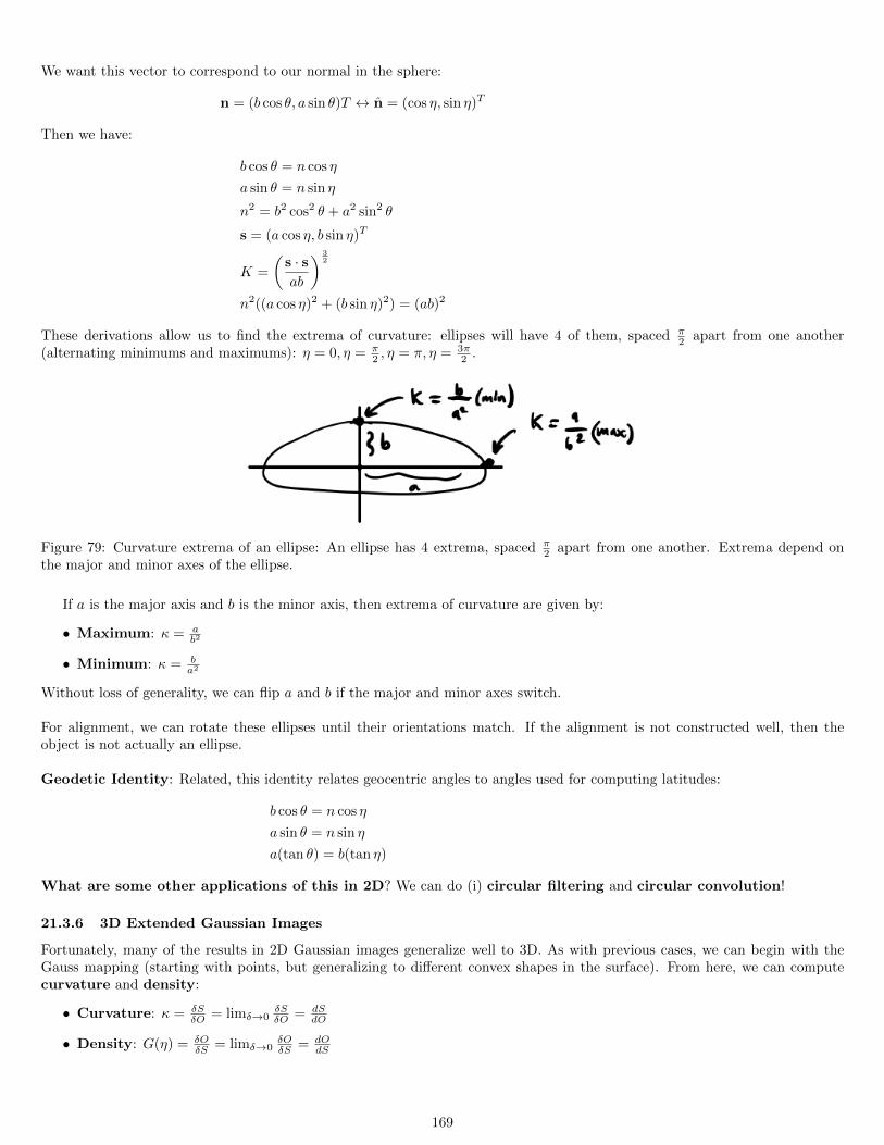
We want this vector to correspond to our normal in the sphere:

n = (b cos θ, a sin θ)T ↔ n = (cos η, sin η)T

Then we have:

b cos θ = n cos η

a sin θ = n sin η

n2 = b2 cos2 θ + a2 sin2 θ

s = (a cos η, b sin η)T

K =

(s · sab

) 32

n2((a cos η)2 + (b sin η)2) = (ab)2

These derivations allow us to find the extrema of curvature: ellipses will have 4 of them, spaced π2 apart from one another

(alternating minimums and maximums): η = 0, η = π2 , η = π, η = 3π

2 .

Figure 79: Curvature extrema of an ellipse: An ellipse has 4 extrema, spaced π2 apart from one another. Extrema depend on

the major and minor axes of the ellipse.

If a is the major axis and b is the minor axis, then extrema of curvature are given by:

• Maximum: κ = ab2

• Minimum: κ = ba2

Without loss of generality, we can flip a and b if the major and minor axes switch.

For alignment, we can rotate these ellipses until their orientations match. If the alignment is not constructed well, then theobject is not actually an ellipse.

Geodetic Identity: Related, this identity relates geocentric angles to angles used for computing latitudes:

b cos θ = n cos η

a sin θ = n sin η

a(tan θ) = b(tan η)

What are some other applications of this in 2D? We can do (i) circular filtering and circular convolution!

21.3.6 3D Extended Gaussian Images

Fortunately, many of the results in 2D Gaussian images generalize well to 3D. As with previous cases, we can begin with theGauss mapping (starting with points, but generalizing to different convex shapes in the surface). From here, we can computecurvature and density:

• Curvature: κ = δSδO = limδ→0

δSδO = dS

dO

• Density: G(η) = δOδS = limδ→0

δOδS = dO

dS

169

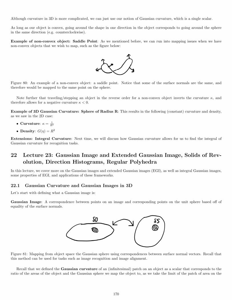
Although curvature in 3D is more complicated, we can just use our notion of Gaussian curvature, which is a single scalar.

As long as our object is convex, going around the shape in one direction in the object corresponds to going around the spherein the same direction (e.g. counterclockwise).

Example of non-convex object: Saddle Point: As we mentioned before, we can run into mapping issues when we havenon-convex objects that we wish to map, such as the figure below:

Figure 80: An example of a non-convex object: a saddle point. Notice that some of the surface normals are the same, andtherefore would be mapped to the same point on the sphere.

Note further that traveling/stepping an object in the reverse order for a non-convex object inverts the curvature κ, andtherefore allows for a negative curvature κ < 0.

Example of 3D Gaussian Curvature: Sphere of Radius R: This results in the following (constant) curvature and density,as we saw in the 2D case:

• Curvature: κ = 1R2

• Density: G(η) = R2

Extensions: Integral Curvature: Next time, we will discuss how Gaussian curvature allows for us to find the integral ofGaussian curvature for recognition tasks.

22 Lecture 23: Gaussian Image and Extended Gaussian Image, Solids of Rev-olution, Direction Histograms, Regular Polyhedra

In this lecture, we cover more on the Gaussian images and extended Gaussian images (EGI), as well as integral Gaussian images,some properties of EGI, and applications of these frameworks.

22.1 Gaussian Curvature and Gaussian Images in 3D

Let’s start with defining what a Gaussian image is:

Gaussian Image: A correspondence between points on an image and corresponding points on the unit sphere based off ofequality of the surface normals.

Figure 81: Mapping from object space the Gaussian sphere using correspondences between surface normal vectors. Recall thatthis method can be used for tasks such as image recognition and image alignment.

Recall that we defined the Gaussian curvature of an (infinitesimal) patch on an object as a scalar that corresponds to theratio of the areas of the object and the Gaussian sphere we map the object to, as we take the limit of the patch of area on the

170

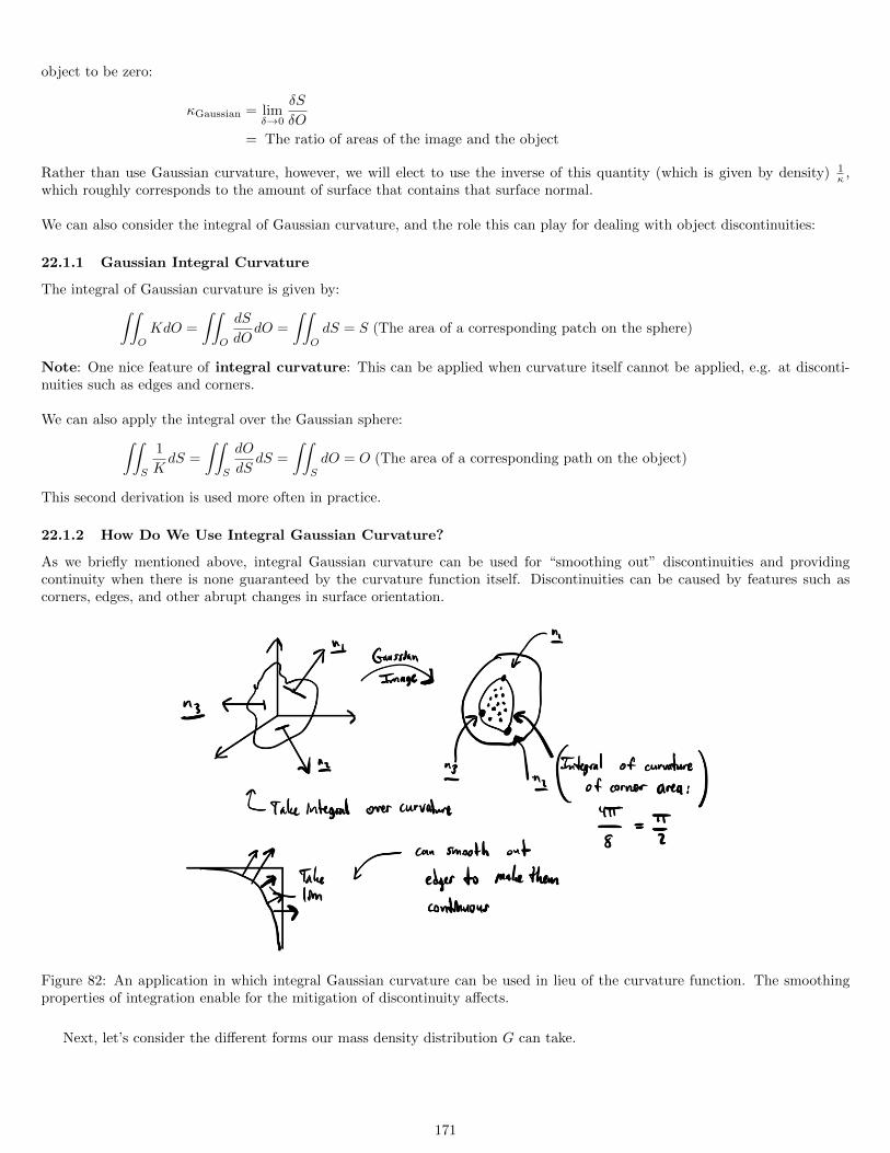
object to be zero:

κGaussian = limδ→0

δS

δO

= The ratio of areas of the image and the object

Rather than use Gaussian curvature, however, we will elect to use the inverse of this quantity (which is given by density) 1κ ,

which roughly corresponds to the amount of surface that contains that surface normal.

We can also consider the integral of Gaussian curvature, and the role this can play for dealing with object discontinuities:

22.1.1 Gaussian Integral Curvature

The integral of Gaussian curvature is given by:∫∫O

KdO =

∫∫O

dS

dOdO =

∫∫O

dS = S (The area of a corresponding patch on the sphere)

Note: One nice feature of integral curvature: This can be applied when curvature itself cannot be applied, e.g. at disconti-nuities such as edges and corners.

We can also apply the integral over the Gaussian sphere:∫∫S

1

KdS =

∫∫S

dO

dSdS =

∫∫S

dO = O (The area of a corresponding path on the object)

This second derivation is used more often in practice.

22.1.2 How Do We Use Integral Gaussian Curvature?

As we briefly mentioned above, integral Gaussian curvature can be used for “smoothing out” discontinuities and providingcontinuity when there is none guaranteed by the curvature function itself. Discontinuities can be caused by features such ascorners, edges, and other abrupt changes in surface orientation.

Figure 82: An application in which integral Gaussian curvature can be used in lieu of the curvature function. The smoothingproperties of integration enable for the mitigation of discontinuity affects.

Next, let’s consider the different forms our mass density distribution G can take.

171

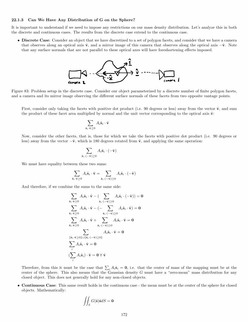
22.1.3 Can We Have Any Distribution of G on the Sphere?

It is important to understand if we need to impose any restrictions on our mass density distribution. Let’s analyze this in boththe discrete and continuous cases. The results from the discrete case extend to the continuous case.

• Discrete Case: Consider an object that we have discretized to a set of polygon facets, and consider that we have a camerathat observes along an optical axis v, and a mirror image of this camera that observes along the optical axis −v. Notethat any surface normals that are not parallel to these optical axes will have foreshortening effects imposed.

Figure 83: Problem setup in the discrete case. Consider our object parameterized by a discrete number of finite polygon facets,and a camera and its mirror image observing the different surface normals of these facets from two opposite vantage points.

First, consider only taking the facets with positive dot product (i.e. 90 degrees or less) away from the vector v, and sumthe product of these facet area multiplied by normal and the unit vector corresponding to the optical axis v:∑

si·v≥0

Aisi · v

Now, consider the other facets, that is, those for which we take the facets with positive dot product (i.e. 90 degrees orless) away from the vector −v, which is 180 degrees rotated from v, and applying the same operation:∑

si·(−v)≥0

Aisi · (−v)

We must have equality between these two sums:∑si·v≥0

Aisi · v =∑

si·(−v)≥0

Aisi · (−v)

And therefore, if we combine the sums to the same side:∑si·v≥0

Aisi · v − (∑

si·(−v)≥0

Aisi · (−v)) = 0

∑si·v≥0

Aisi · v − (−∑

si·(−v)≥0

Aisi · v) = 0

∑si·v≥0

Aisi · v +∑

si·(−v)≥0

Aisi · v = 0

∑si·v≥0∪si·(−v)≥0

Aisi · v = 0

∑i

Aisi · v = 0

(∑i

Aisi) · v = 0 ∀ v

Therefore, from this it must be the case that∑iAisi = 0, i.e. that the center of mass of the mapping must be at the

center of the sphere. This also means that the Gaussian density G must have a “zero-mean” mass distribution for anyclosed object. This does not generally hold for any non-closed objects.

• Continuous Case: This same result holds in the continuous case - the mean must be at the center of the sphere for closedobjects. Mathematically: ∫∫

S

G(s)sdS = 0

172

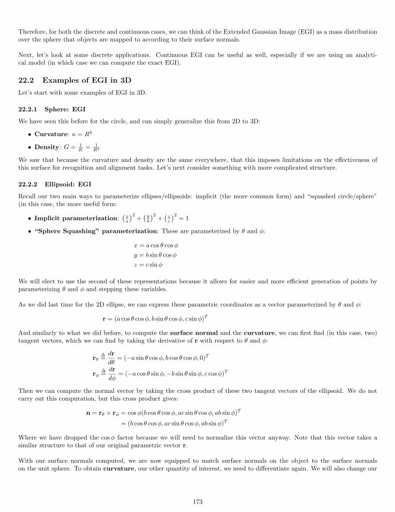
Therefore, for both the discrete and continuous cases, we can think of the Extended Gaussian Image (EGI) as a mass distributionover the sphere that objects are mapped to according to their surface normals.

Next, let’s look at some discrete applications. Continuous EGI can be useful as well, especially if we are using an analyti-cal model (in which case we can compute the exact EGI).

22.2 Examples of EGI in 3D

Let’s start with some examples of EGI in 3D.

22.2.1 Sphere: EGI

We have seen this before for the circle, and can simply generalize this from 2D to 3D:

• Curvature: κ = R2

• Density: G = 1K = 1

R2

We saw that because the curvature and density are the same everywhere, that this imposes limitations on the effectiveness ofthis surface for recognition and alignment tasks. Let’s next consider something with more complicated structure.

22.2.2 Ellipsoid: EGI

Recall our two main ways to parameterize ellipses/ellipsoids: implicit (the more common form) and “squashed circle/sphere”(in this case, the more useful form:

• Implicit parameterization:(xa

)2+(yb

)2+(zc

)2= 1

• “Sphere Squashing” parameterization: These are parameterized by θ and φ:

x = a cos θ cosφ

y = b sin θ cosφ

z = c sinφ

We will elect to use the second of these representations because it allows for easier and more efficient generation of points byparameterizing θ and φ and stepping these variables.

As we did last time for the 2D ellipse, we can express these parametric coordinates as a vector parameterized by θ and φ:

r = (a cos θ cosφ, b sin θ cosφ, c sinφ)T

And similarly to what we did before, to compute the surface normal and the curvature, we can first find (in this case, two)tangent vectors, which we can find by taking the derivative of r with respect to θ and φ:

rθ∆=dr

dθ= (−a sin θ cosφ, b cos θ cosφ, 0)T

rφ∆=dr

dφ= (−a cos θ sinφ,−b sin θ sinφ, c cosφ)T

Then we can compute the normal vector by taking the cross product of these two tangent vectors of the ellipsoid. We do notcarry out this computation, but this cross product gives:

n = rθ × rφ = cosφ(b cos θ cosφ, ac sin θ cosφ, ab sinφ)T

= (b cos θ cosφ, ac sin θ cosφ, ab sinφ)T

Where we have dropped the cosφ factor because we will need to normalize this vector anyway. Note that this vector takes asimilar structure to that of our original parametric vector r.

With our surface normals computed, we are now equipped to match surface normals on the object to the surface normalson the unit sphere. To obtain curvature, our other quantity of interest, we need to differentiate again. We will also change our

173

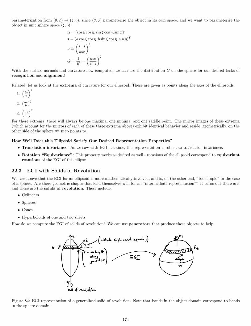
parameterization from (θ, φ) → (ξ, η), since (θ, φ) parameterize the object in its own space, and we want to parameterize theobject in unit sphere space (ξ, η).

n = (cos ξ cos η, sin ξ cos η, sin η)T

s = (a cos ξ cos η, b sin ξ cos η, sin η)T

κ =

(s · sabc

)2

G =1

K=

(abc

s · s

)2

With the surface normals and curvature now computed, we can use the distribution G on the sphere for our desired tasks ofrecognition and alignment!

Related, let us look at the extrema of curvature for our ellipsoid. These are given as points along the axes of the ellipsoids:

1.(bca

)2

2.(acb

)23.(abc

)2

For these extrema, there will always be one maxima, one minima, and one saddle point. The mirror images of these extrema(which account for the mirrors of each of these three extrema above) exhibit identical behavior and reside, geometrically, on theother side of the sphere we map points to.

How Well Does this Ellipsoid Satisfy Our Desired Representation Properties?

• Translation invariance: As we saw with EGI last time, this representation is robust to translation invariance.

• Rotation “Equivariance”: This property works as desired as well - rotations of the ellipsoid correspond to equivariantrotations of the EGI of this ellipse.

22.3 EGI with Solids of Revolution

We saw above that the EGI for an ellipsoid is more mathematically-involved, and is, on the other end, “too simple” in the caseof a sphere. Are there geometric shapes that lend themselves well for an “intermediate representation”? It turns out there are,and these are the solids of revolution. These include:

• Cylinders

• Spheres

• Cones

• Hyperboloids of one and two sheets

How do we compute the EGI of solids of revolution? We can use generators that produce these objects to help.

Figure 84: EGI representation of a generalized solid of revolution. Note that bands in the object domain correspond to bandsin the sphere domain.

174

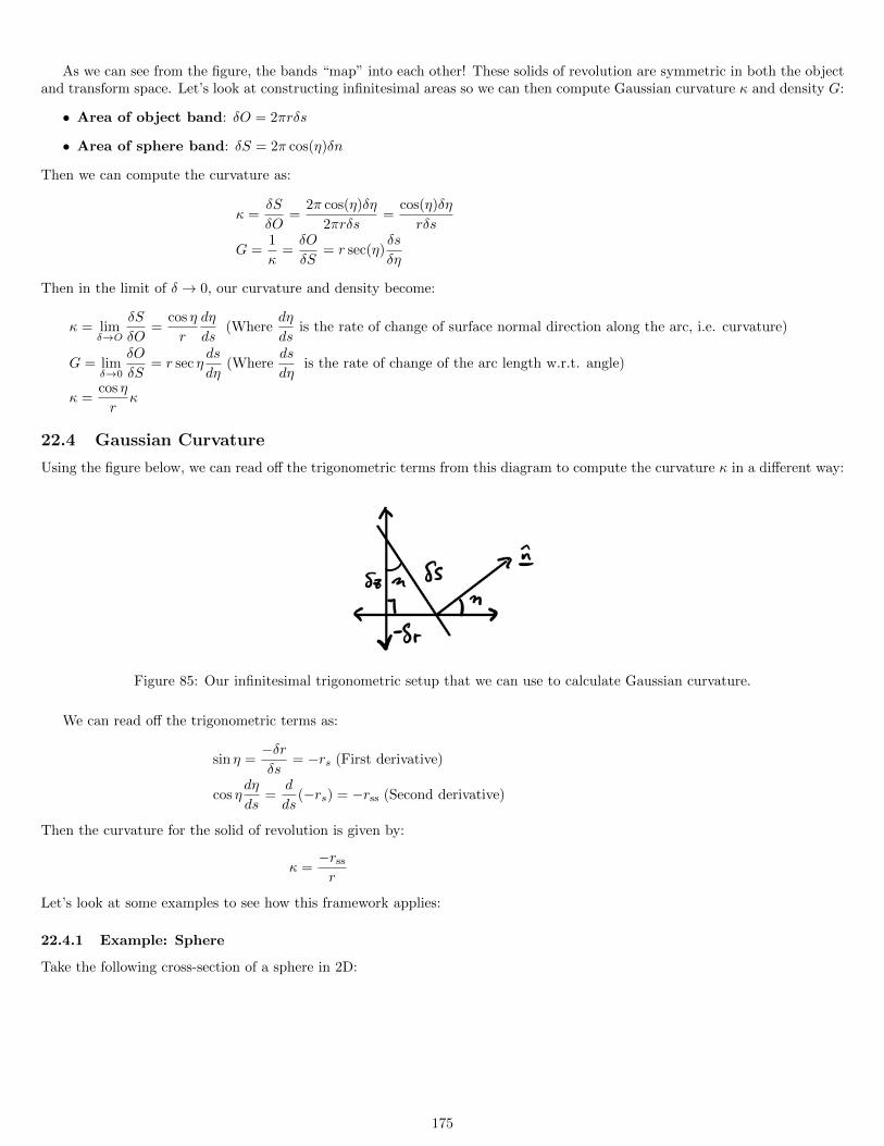
As we can see from the figure, the bands “map” into each other! These solids of revolution are symmetric in both the objectand transform space. Let’s look at constructing infinitesimal areas so we can then compute Gaussian curvature κ and density G:

• Area of object band: δO = 2πrδs

• Area of sphere band: δS = 2π cos(η)δn

Then we can compute the curvature as:

κ =δS

δO=

2π cos(η)δη

2πrδs=

cos(η)δη

rδs

G =1

κ=δO

δS= r sec(η)

δs

δη

Then in the limit of δ → 0, our curvature and density become:

κ = limδ→O

δS

δO=

cos η

r

dη

ds(Where

dη

dsis the rate of change of surface normal direction along the arc, i.e. curvature)

G = limδ→0

δO

δS= r sec η

ds

dη(Where

ds

dηis the rate of change of the arc length w.r.t. angle)

κ =cos η

rκ

22.4 Gaussian Curvature

Using the figure below, we can read off the trigonometric terms from this diagram to compute the curvature κ in a different way:

Figure 85: Our infinitesimal trigonometric setup that we can use to calculate Gaussian curvature.

We can read off the trigonometric terms as:

sin η =−δrδs

= −rs (First derivative)

cos ηdη

ds=

d

ds(−rs) = −rss (Second derivative)

Then the curvature for the solid of revolution is given by:

κ =−rss

r

Let’s look at some examples to see how this framework applies:

22.4.1 Example: Sphere

Take the following cross-section of a sphere in 2D:

175

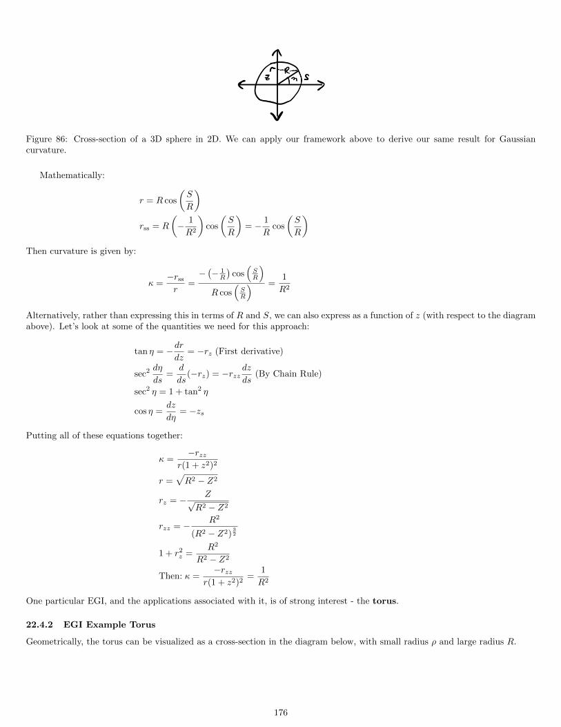
Figure 86: Cross-section of a 3D sphere in 2D. We can apply our framework above to derive our same result for Gaussiancurvature.

Mathematically:

r = R cos

(S

R

)rss = R

(− 1

R2

)cos

(S

R

)= − 1

Rcos

(S

R

)Then curvature is given by:

κ =−rss

r=−(− 1R

)cos(SR

)R cos

(SR

) =1

R2

Alternatively, rather than expressing this in terms of R and S, we can also express as a function of z (with respect to the diagramabove). Let’s look at some of the quantities we need for this approach:

tan η = −drdz

= −rz (First derivative)

sec2 dη

ds=

d

ds(−rz) = −rzz

dz

ds(By Chain Rule)

sec2 η = 1 + tan2 η

cos η =dz

dη= −zs

Putting all of these equations together:

κ =−rzz

r(1 + z2)2

r =√R2 − Z2

rz = − Z√R2 − Z2

rzz = − R2

(R2 − Z2)32

1 + r2z =

R2

R2 − Z2

Then: κ =−rzz

r(1 + z2)2=

1

R2

One particular EGI, and the applications associated with it, is of strong interest - the torus.

22.4.2 EGI Example Torus

Geometrically, the torus can be visualized as a cross-section in the diagram below, with small radius ρ and large radius R.

176

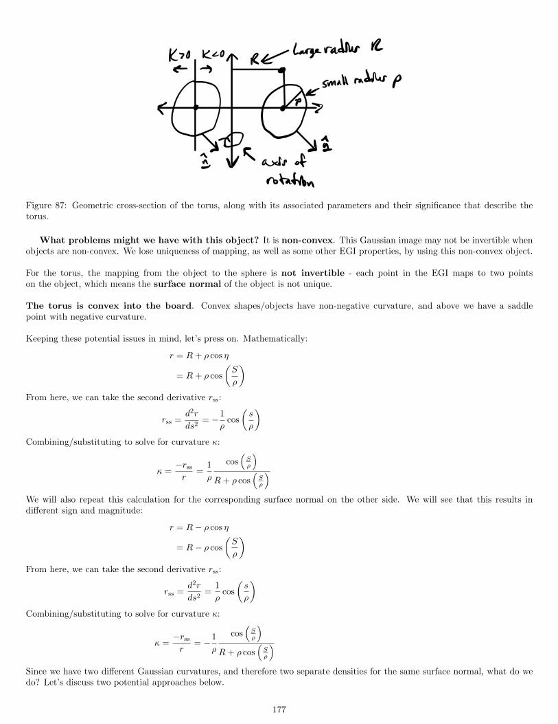
Figure 87: Geometric cross-section of the torus, along with its associated parameters and their significance that describe thetorus.

What problems might we have with this object? It is non-convex. This Gaussian image may not be invertible whenobjects are non-convex. We lose uniqueness of mapping, as well as some other EGI properties, by using this non-convex object.

For the torus, the mapping from the object to the sphere is not invertible - each point in the EGI maps to two pointson the object, which means the surface normal of the object is not unique.

The torus is convex into the board. Convex shapes/objects have non-negative curvature, and above we have a saddlepoint with negative curvature.

Keeping these potential issues in mind, let’s press on. Mathematically:

r = R+ ρ cos η

= R+ ρ cos

(S

ρ

)From here, we can take the second derivative rss:

rss =d2r

ds2= −1

ρcos

(s

ρ

)Combining/substituting to solve for curvature κ:

κ =−rss

r=

1

ρ

cos(Sρ

)R+ ρ cos

(Sρ

)We will also repeat this calculation for the corresponding surface normal on the other side. We will see that this results indifferent sign and magnitude:

r = R− ρ cos η

= R− ρ cos

(S

ρ

)From here, we can take the second derivative rss:

rss =d2r

ds2=

1

ρcos

(s

ρ

)Combining/substituting to solve for curvature κ:

κ =−rss

r= −1

ρ

cos(Sρ

)R+ ρ cos

(Sρ

)Since we have two different Gaussian curvatures, and therefore two separate densities for the same surface normal, what do wedo? Let’s discuss two potential approaches below.

177

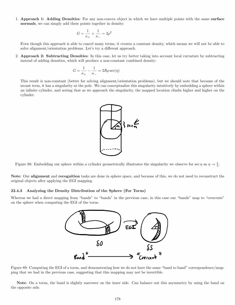
1. Approach 1: Adding Densities: For any non-convex object in which we have multiple points with the same surfacenormals, we can simply add these points together in density:

G =1

κ++

1

κ−= 2ρ2

Even though this approach is able to cancel many terms, it creates a constant density, which means we will not be able tosolve alignment/orientation problems. Let’s try a different approach.

2. Approach 2: Subtracting Densities: In this case, let us try better taking into account local curvature by subtractinginstead of adding densities, which will produce a non-constant combined density:

G =1

κ+− 1

κ−= 2Rρ sec(η)

This result is non-constant (better for solving alignment/orientation problems), but we should note that because of thesecant term, it has a singularity at the pole. We can conceptualize this singularity intuitively by embedding a sphere withinan infinite cylinder, and noting that as we approach the singularity, the mapped location climbs higher and higher on thecylinder.

Figure 88: Embedding our sphere within a cylinder geometrically illustrates the singularity we observe for sec η as η → π2 .

Note: Our alignment and recognition tasks are done in sphere space, and because of this, we do not need to reconstruct theoriginal objects after applying the EGI mapping.

22.4.3 Analyzing the Density Distribution of the Sphere (For Torus)

Whereas we had a direct mapping from “bands” to “bands” in the previous case, in this case our “bands” map to “crescents”on the sphere when computing the EGI of the torus.

Figure 89: Computing the EGI of a torus, and demonstrating how we do not have the same “band to band” correspondence/map-ping that we had in the previous case, suggesting that this mapping may not be invertible.

Note: On a torus, the band is slightly narrower on the inner side. Can balance out this asymmetry by using the band onthe opposite side.

178

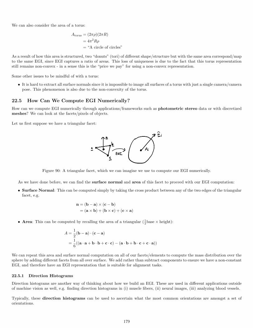
We can also consider the area of a torus:

Atorus = (2πρ)(2πR)

= 4π2Rρ

= “A circle of circles”

As a result of how this area is structured, two “donuts” (tori) of different shape/structure but with the same area correspond/mapto the same EGI, since EGI captures a ratio of areas. This loss of uniqueness is due to the fact that this torus representationstill remains non-convex - in a sense this is the “price we pay” for using a non-convex representation.

Some other issues to be mindful of with a torus:

• It is hard to extract all surface normals since it is impossible to image all surfaces of a torus with just a single camera/camerapose. This phenomenon is also due to the non-convexity of the torus.

22.5 How Can We Compute EGI Numerically?

How can we compute EGI numerically through applications/frameworks such as photometric stereo data or with discretizedmeshes? We can look at the facets/pixels of objects.

Let us first suppose we have a triangular facet:

Figure 90: A triangular facet, which we can imagine we use to compute our EGI numerically.

As we have done before, we can find the surface normal and area of this facet to proceed with our EGI computation:

• Surface Normal: This can be computed simply by taking the cross product between any of the two edges of the triangularfacet, e.g.

n = (b− a)× (c− b)

= (a× b) + (b× c) + (c× a)

• Area: This can be computed by recalling the area of a triangular (12base× height):

A =1

2(b− a) · (c− a)

=1

6((a · a + b · b + c · c)− (a · b + b · c + c · a))

We can repeat this area and surface normal computation on all of our facets/elements to compute the mass distribution over thesphere by adding different facets from all over surface. We add rather than subtract components to ensure we have a non-constantEGI, and therefore have an EGI representation that is suitable for alignment tasks.

22.5.1 Direction Histograms

Direction histograms are another way of thinking about how we build an EGI. These are used in different applications outsideof machine vision as well, e.g. finding direction histograms in (i) muscle fibers, (ii) neural images, (iii) analyzing blood vessels.

Typically, these direction histograms can be used to ascertain what the most common orientations are amongst a set oforientations.

179

For histograms in higher dimensions, is subdividing the region into squares/cubes the most effective approach? As it turnsout, no, and this is because the regions are not round. We would prefer to fill in the plane with disks.

To contrast, suppose the tessellation is with triangles - you are now combining things that are pretty far away, comparedto a square. Hexagons alleviate this problem by minimizing distance from the center of each cell to the vertives, while alsopreventing overlapping/not filled in regions. Other notes:

• We also need to take “randomness” into account, i.e. when points lie very close to the boundaries between different bins.We can account for this phenomena by constructing and counting not only the original grids, but additionally, shifted/offsetgrids that adjust the intervals, and consequently the counts in each grid cell.

The only issue with this approach is that this “solution” scales poorly with dimensionality: As we increase dimensions, weneed to take more grids (e.g. for 2D, we need our (i) Original plane, (ii) Shifted x, (iii) Shifted y, and (iv) Shifted x andshifted y). However, in light of this, this is a common solution approach for mitigating “randomness” in 2D binning.

22.5.2 Desired Properties of Dividing Up the Sphere/Tessellations

To build an optimal representation, we need to understand what our desired optimal properties of our tessellations will be:

1. Equal areas of cells/facets

2. Equal shapes of cells/facets

3. “Rounded” shapes of cells/facets

4. Regular pattern

5. Allows for easy “binning”: As an example a brute force way to do binning for spheres is to compute the dotr productwith all surface normals and take the largest of these. This is very impractical and computationally-inefficient because itrequires us to step through all data each time. For this reason, it is important we consider implementations/representationsthat make binning efficient and straightforward.

6. Alignment of rotation: The idea with this is that we need to bring one object into alignment with the other in order todo effective recognition, one of the key tasks we cited.

For instance, with a dodecahedron, our orientation/direction histogram is represented by 12 numbers (which cor-respond to the number of faces on the dodecahedron):

[A1, A2, · · · , A12]

When we bring this object into alignment during, for instance, a recognition task, we merely only need to permute theorder of these 12 numbers - all information is preserved and there is no loss from situations such as overlapping. This isan advantage of having alignment of rotation.

[A7, A4, · · · , A8]

Platonic and Archimedean solids are the representations we will use for these direction histograms.

23 Quiz 1 Review

Here you will find a review of some of the topics covered so far in Machine Vision. These are as follows in the section notes:

1. Mathematics review - Unconstrained optimization, Green’s Theorem, Bezout’s Theorem, Nyquist Sampling Theorem

2. Projection - Perspective vs. Orthographic, Object vs. Image space

3. Optical Flow - BCCE/optical flow, Time to Contact, vanishing points

4. Photometry - Radiance, irradiance, illumination, geometry, BRDF, Helmholtz Reciprocity

5. Different surface types - Lambertian, Hapke

6. Shape from Shading (SfS) - Hapke case, general case, reflectance maps, image irradiance equation

180

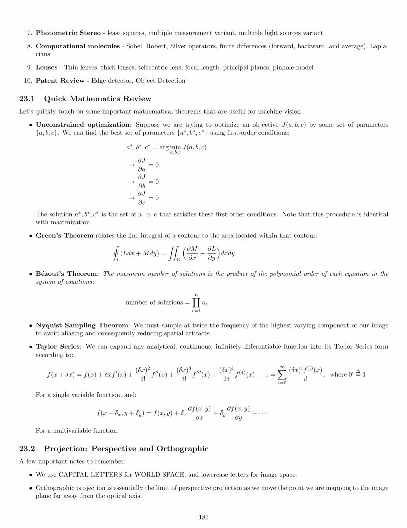
7. Photometric Stereo - least squares, multiple measurement variant, multiple light sources variant

8. Computational molecules - Sobel, Robert, Silver operators, finite differences (forward, backward, and average), Lapla-cians

9. Lenses - Thin lenses, thick lenses, telecentric lens, focal length, principal planes, pinhole model

10. Patent Review - Edge detector, Object Detection

23.1 Quick Mathematics Review

Let’s quickly touch on some important mathematical theorems that are useful for machine vision.

• Unconstrained optimization: Suppose we are trying to optimize an objective J(a, b, c) by some set of parametersa, b, c. We can find the best set of parameters a∗, b∗, c∗ using first-order conditions:

a∗, b∗, c∗ = arg mina,b,c

J(a, b, c)

→ ∂J

∂a= 0

→ ∂J

∂b= 0

→ ∂J

∂c= 0

The solution a∗, b∗, c∗ is the set of a, b, c that satisfies these first-order conditions. Note that this procedure is identicalwith maximization.

• Green’s Theorem relates the line integral of a contour to the area located within that contour:∮L

(Ldx+Mdy) =

∫∫D

(∂M∂x− ∂L

∂y

)dxdy

• Bezout’s Theorem: The maximum number of solutions is the product of the polynomial order of each equation in thesystem of equations:

number of solutions =E∏e=1

oe

• Nyquist Sampling Theorem: We must sample at twice the frequency of the highest-varying component of our imageto avoid aliasing and consequently reducing spatial artifacts.

• Taylor Series: We can expand any analytical, continuous, infinitely-differentiable function into its Taylor Series formaccording to:

f(x+ δx) = f(x) + δxf ′(x) +(δx)2

2!f ′′(x) +

(δx)3

3!f ′′′(x) +

(δx)4

24f (4)(x) + ... =

∞∑i=0

(δx)if (i)(x)

i!, where 0!

∆= 1

For a single variable function, and:

f(x+ δx, y + δy) = f(x, y) + δx∂f(x, y)

∂x+ δy

∂f(x, y)

∂y+ · · ·

For a multivariable function.

23.2 Projection: Perspective and Orthographic

A few important notes to remember:

• We use CAPITAL LETTERS for WORLD SPACE, and lowercase letters for image space.

• Orthographic projection is essentially the limit of perspective projection as we move the point we are mapping to the imageplane far away from the optical axis.

181

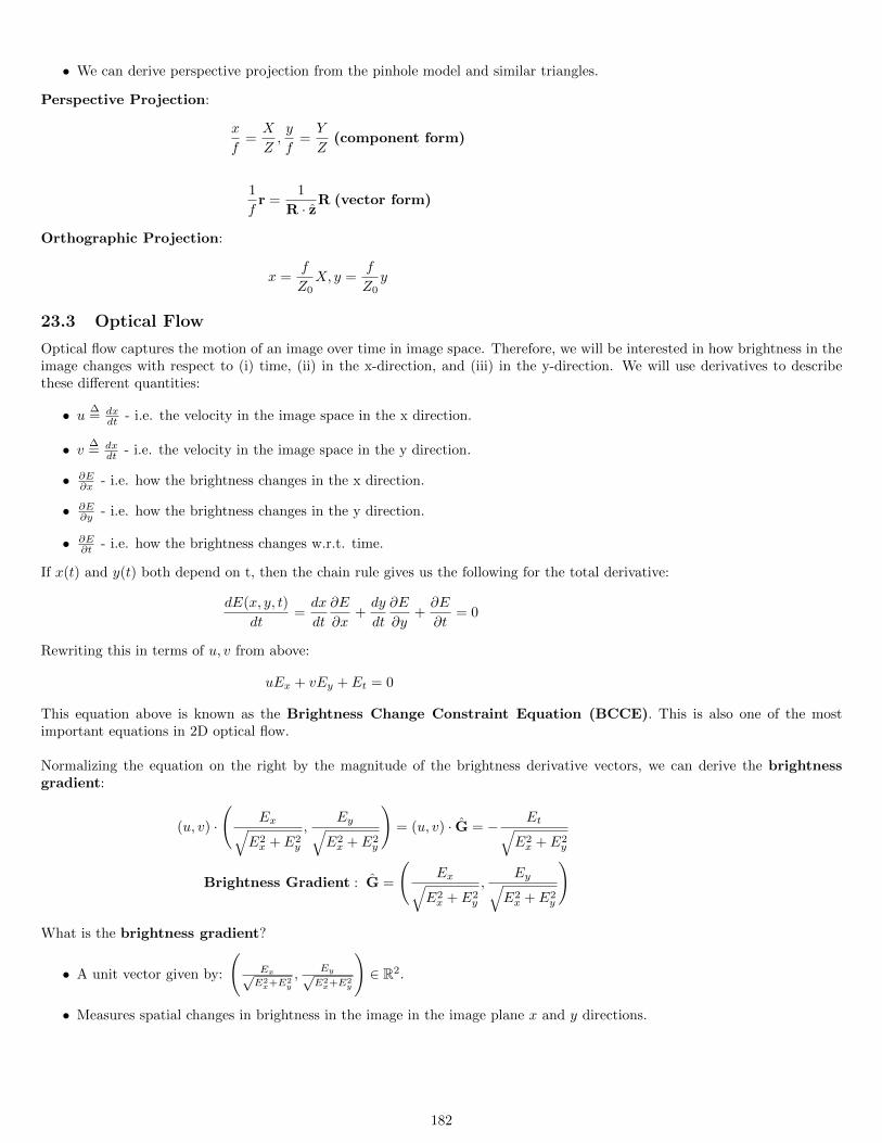
• We can derive perspective projection from the pinhole model and similar triangles.

Perspective Projection:

x

f=X

Z,y

f=Y

Z(component form)

1

fr =

1

R · zR (vector form)

Orthographic Projection:

x =f

Z0X, y =

f

Z0y

23.3 Optical Flow

Optical flow captures the motion of an image over time in image space. Therefore, we will be interested in how brightness in theimage changes with respect to (i) time, (ii) in the x-direction, and (iii) in the y-direction. We will use derivatives to describethese different quantities:

• u ∆= dx

dt - i.e. the velocity in the image space in the x direction.

• v ∆= dx

dt - i.e. the velocity in the image space in the y direction.

• ∂E∂x - i.e. how the brightness changes in the x direction.

• ∂E∂y - i.e. how the brightness changes in the y direction.

• ∂E∂t - i.e. how the brightness changes w.r.t. time.

If x(t) and y(t) both depend on t, then the chain rule gives us the following for the total derivative:

dE(x, y, t)

dt=dx

dt

∂E

∂x+dy

dt

∂E

∂y+∂E

∂t= 0

Rewriting this in terms of u, v from above:

uEx + vEy + Et = 0

This equation above is known as the Brightness Change Constraint Equation (BCCE). This is also one of the mostimportant equations in 2D optical flow.

Normalizing the equation on the right by the magnitude of the brightness derivative vectors, we can derive the brightnessgradient:

(u, v) ·

(Ex√

E2x + E2

y

,Ey√

E2x + E2

y

)= (u, v) · G = − Et√

E2x + E2

y

Brightness Gradient : G =

(Ex√

E2x + E2

y

,Ey√

E2x + E2

y

)

What is the brightness gradient?

• A unit vector given by:

(Ex√E2x+E2

y

,Ey√E2x+E2

y

)∈ R2.

• Measures spatial changes in brightness in the image in the image plane x and y directions.

182

We are also interested in contours of constant brightness, or isophotes. These are curves on an illuminated surface that connectspoints of equal brightness (source: Wikipedia).

Finally, we are also interested in solving for optimal values of u and v for multiple measurements. In the ideal case with-out noise: [

UV

]=

1

(Ex1Ey2 − Ey1Ex2

)

[Ey2 −Ey1−Ex2

Ex1

] [−Et1−Et2

]

When there is noise we simply minimize our objective, instead of setting it equal to zero:

J(u, v)∆=

∫x∈X

∫y∈Y

(uEx + vEy + Et)2dxdy

We solve for our set of optimal parameters by finding the set of parameters that minimizes this objective:

u∗, v∗ = arg minu,v

J(u, v) = arg minu,v

∫x∈X

∫y∈Y

(uEx + vEy + Et)2dxdy

Since this is an unconstrained optimization problem, we can solve by finding the minimum of the two variables using twoFirst-Order Conditions (FOCs):

• ∂J(u,v)∂u = 0

• ∂J(u,v)∂v = 0

Vanishing points: These are the points in the image plane (or extended out from the image plane) that parallel lines in theworld converge to. Applications include:

• Multilateration

• Calibration Objects (Sphere, Cube)

• Camera Calibration

We will also look at Time to Contact (TTC):

Z

W

∆==

ZdZdt

=metersmetersseconds

= seconds

Let us express the inverse of this Time to Contact (TTC) quantity as C, which can be interpreted roughly as the number offrames until contact is made:

C∆=W

Z=

1

TTC

23.4 Photometry

Here, we will mostly focus on some of the definitions we have encountered from lecture:

• Photometry: Photometry is the science of measuring visible radiation, light, in units that are weighted according to thesensitivity of the human eye. It is a quantitative science based on a statistical model of the human visual perception oflight (eye sensitivity curve) under carefully controlled conditions.

• Radiometry: Radiometry is the science of measuring radiation energy in any portion of the electromagnetic spectrum.In practice, the term is usually limited to the measurement of ultraviolet (UV), visible (VIS), and infrared (IR) radiationusing optical instruments.

• Irradiance: E∆= δP

δA (W/m2). This corresponds to light falling on a surface. When imaging an object, irradiance isconverted to a grey level.

• Intensity: I∆= δP

δW (W/ster). This quantity applied to a point source and is often directionally-dependent.

• Radiance: L∆= δ2P

δAδΩ (W/m2× ster). This photometric quantity is a measure of how bright a surface appears in an image.

183

• BRDF (Bidirectional Reflectance Distribution): f(θi, θe, φi, φe) = δL(θe,φe)δE(θi,φi)

. This function captures the fact that

oftentimes, we are only interested in light hitting the camera, as opposed to the total amount of light emitted from anobject. Last time, we had the following equation to relate image irradiance with object/surface radiance:

E =π

4L( df

)2

cos4 α

Where the irradiance of the image E is on the lefthand side and the radiance of the object/scene L is on the right. TheBRDF must also satisfy Helmholtz reciprocity, otherwise we would be violating the 2nd Law of Thermodynamics.Mathematically, recall that Helmholtz reciprocity is given by:

f(θi, θe, φi, φe) = f(θe, θi, φe, φi) ∀ θi, θe, φi, φe

23.5 Different Surface Types

With many of our photometric properties established, we can also discuss photometric properties of different types of surfaces.Before we dive in, it is important to also recall the definition of surface orientation:

• p ∆= ∂z

∂x

• q ∆= ∂z

∂y

• Lambertian Surfaces:

– Ideal Lambertian surfaces are equally bright from all directions, i.e.

f(θi, θe, φi, φe) = f(θe, θi, φe, φi) ∀ θi, θe, φi, φeAND

f(θi, θe, φi, φe) = K ∈ R with respect to θe, φe

– “Lambert’s Law”:

Ei ∝ cos θi = n · si

• Hapke Surfaces:

– The BRDF of a Hapke surface is given by:

f(θi, φi, θe, φe) =1√

cos θe cos θi

– Isophotes of Hapke surfaces are linear in spatial gradient, or (p, q) space.

• What do the isophotes of the moon look like, supposing the moon can fall under some of the different types of surfaces wehave discussed?

– Lambertian: We will see circles and ellipses of isophotes, depending on the angle made between the viewer and thethe moon.

– Hapke: Because of the BRDF behavior, isophotes will run longitudinally along the moon in the case in which it isa Hapke surface.

23.6 Shape from Shading (SfS)

This is one of the most fundamental problems in machine vision in which we try to estimate the surface of an object frombrightness measurements. Several variations of this problem we consider:

• Hapke surfaces - this leads to linear isophotes in (p, q) space, and allows us to solve for one of the dimensions of interest.

• General case: There are several techniques we can apply to solve for this:

– Green’s Theorem (see lecture notes handout)

– Iterative Discrete Optimization (see lecture notes handout)

184

For these problems, we considered:

– Characteristic strips (x, y, z, p, q)

– Initial curves/base characteristics

– Normalizing with respect to constant step sizes

– A system of 5 ODEs

– Stationary points and estimates of surfaces around them for initial points

Next, let us review reflectance maps. A reflectance map R(p, q) is a lookup table (or, for simpler cases, a parametric function)that stores the brightness for particular surface orientations p = ∂z

∂x , q = ∂z∂y .

The Image Irradiance Equation relates the reflectance map to the brightness function in the image E(x, y) and is thefirst step in many Shape from Shading approaches.

E(x, y) = R(p, q)

23.7 Photometric Stereo

Photometric stereo is a technique in machine vision for estimating the surface normals of objects by observing that objectunder different lighting conditions. This problem is quite common in machine vision applications.

One way we can solve photometric stereo is by taking multiple brightness measurements from a light source that we movearound. This problem becomes: −sT1−sT2

−sT3

n =

E1

E2

E3

Written compactly:

Sn = E −→ n = S−1E

Note that we we need S to be invertible to compute this, which occurs when the light source vectors are not coplanar.

Other variations of this problem:

• Using light sources at different electromagnetic frequencies

• Using a camera with different light filters

• Moving the object to different locations

23.8 Computational Molecules

These are crucial components for applying machine concepts to real-life problems.

1. Ex = 1ε (E(x, y)− E(x− 1, y)) (Backward Difference), 1

ε (z(x+ 1, y)− z(x, y)) (Forward Difference)

2. Ey = 1ε (E(x, y)− E(x, y − 1)) (Backward Difference), 1

ε (E(x, y + 1)− E(x, y)) (Forward Difference)

3. ∆E = ∇2E = 1ε2 (4E(x, y)− (E(x− 1, y) + E(x+ 1, y) + E(x, y − 1) + E(x, y + 1)))

4. Exx = ∂2E∂x2 = 1

ε2 (E(x− 1, y)− 2(x, y) + E(x+ 1, y))

5. Eyy = ∂2z∂y2 = 1

ε2 (E(x, y − 1)− 2(x, y) + E(x, y + 1))

6. Robert’s Cross: This approximates derivatives in a coordinate system rotated 45 degrees (x′, y′). The derivatives canbe approximated using the Kx′ and Ky′ kernels:

∂E

∂x′→ Kx′ =

[0 −1−1 0

]∂E

∂y′→ Ky′ =

[1 00 −1

]

185

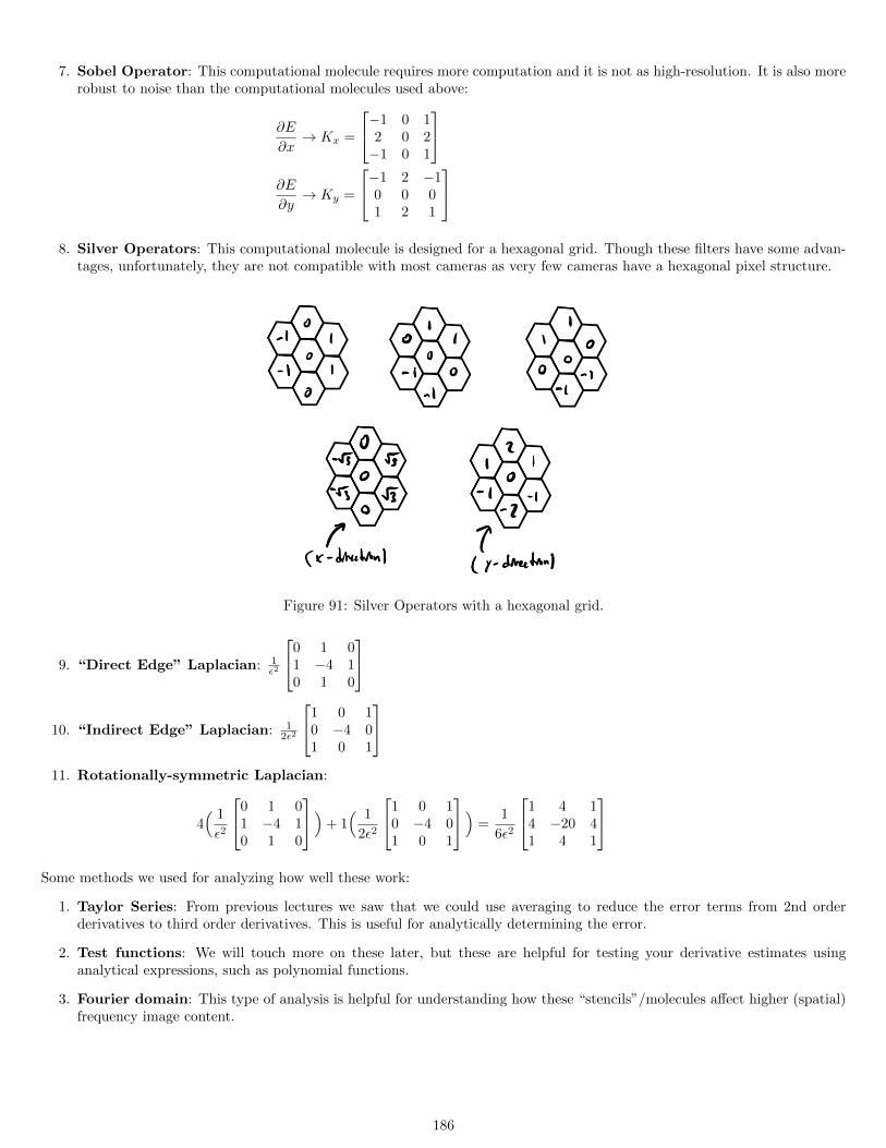
7. Sobel Operator: This computational molecule requires more computation and it is not as high-resolution. It is also morerobust to noise than the computational molecules used above:

∂E

∂x→ Kx =

−1 0 12 0 2−1 0 1

∂E

∂y→ Ky =

−1 2 −10 0 01 2 1

8. Silver Operators: This computational molecule is designed for a hexagonal grid. Though these filters have some advan-

tages, unfortunately, they are not compatible with most cameras as very few cameras have a hexagonal pixel structure.

Figure 91: Silver Operators with a hexagonal grid.

9. “Direct Edge” Laplacian: 1ε2

0 1 01 −4 10 1 0

10. “Indirect Edge” Laplacian: 12ε2

1 0 10 −4 01 0 1

11. Rotationally-symmetric Laplacian:

4( 1

ε2

0 1 01 −4 10 1 0

)+ 1( 1

2ε2

1 0 10 −4 01 0 1

) =1

6ε2

1 4 14 −20 41 4 1

Some methods we used for analyzing how well these work:

1. Taylor Series: From previous lectures we saw that we could use averaging to reduce the error terms from 2nd orderderivatives to third order derivatives. This is useful for analytically determining the error.

2. Test functions: We will touch more on these later, but these are helpful for testing your derivative estimates usinganalytical expressions, such as polynomial functions.

3. Fourier domain: This type of analysis is helpful for understanding how these “stencils”/molecules affect higher (spatial)frequency image content.

186

23.9 Lenses

Lenses are also important, because they determine our ability to sense light and perform important machine vision applications.Some types of lenses:

• Thin lenses are the first type of lens we consider. These are often made from glass spheres, and obey the following threerules:

– Central rays (rays that pass through the center of the lens) are undeflected - this allows us to preserve perspectiveprojection as we had for pinhole cameras.

– The ray from the focal center emerges parallel to the optical axis.

– Any parallel rays go through the focal center.

• Thick lenses (cascaded thin lenses)

• Telecentric lenses - These “move” the the Center of Projection to infinity to achieve approximately orthographic pro-jection.

• Potential distortions caused by lenses:

– Radial distortion: In order to bring the entire angle into an image (e.g. for wide-angle lenses), we have the “squash”the edges of the solid angle, thus leading to distortion that is radially-dependent. Typically, other lens defects aremitigated at the cost of increased radial distortion. Some specific kinds of radial distortion [5]:

∗ Barrel distortion

∗ Mustache distortion

∗ Pincushion distortion

– Lens Defects: These occur frequently when manufacturing lenses, and can originate from a multitude of differentissues.

23.10 Patent Review

The two patents we touched on were for:

• Fast and Accurate Edge detection: At a high level, this framework leveraged the following steps for fast edge detection:

– CORDIC algorithm for estimating (and subsequently quantizing) the brightness gradient direction

– Thresholding gradients via Non-Maximum Suppression (NMS)

– Interpolation at the sub-pixel level along with peak finding for accurate edge detection at sub-pixel level

– Bias compensation

– Plane position

We also discussed some issues/considerations with the following aspects of this framework’s design:

– Quantization of gradient direction

– Interpolation method for sub-pixel accuracy (quadratic, piecewise linear, cubic, etc.)

• Object detection and pose estimation: At a high level, this framework leveraged the following steps for fast objectdetection/pose estimation:

– Finding specific probing points in a template image that we use for comparing/estimating gradients.

– Using different scoring functions to compare template image to different configurations of the runtime image tofind the object along with its pose (position with orientation).

Here you will find a high-level review of some of the topics covered since Quiz 1. These are as follows in the section notes:

1. Relevant Mathematics Review - Rayleigh Quotients, Groups, Levenberg-Marquadt, Bezout’s Theorem

2. Systems/Patents - PatQuick, PatMAx, Fast Convolutions, Hough Transforms

3. Signals - Sampling, Spline Interpolation, Integral Images, Repeated Block Averaging

4. Photogrammetry - Photogrammetry Problems, Absolute orientation, Relative Orientation, Interior Orientation, ExteriorOrientation, Critical Surfaces, Radial and Tangential Distortion

5. Rotations/Orientation - Gibb’s vector, Rodrigues Formula, Quaternions, Orthonormal Matrices

6. 3D Recognition - Extended Gaussian Image, Solids of Revolution, Polyhedral Objects, Desirable Properties

187

24 Quiz 2 Review

24.1 Relevant Mathematics Review

We’ll start with a review of some of the relevant mathematical tools we have relied on in the second part of the course.

24.1.1 Rayleigh Quotients

We saw from our lectures with absolute orientation that this is a simpler way (relative to Lagrange Multipliers) to take con-straints into account:

The intuitive idea behind them: How do I prevent my parameters from becoming too large) positive or negative) or too small(zero)? We can accomplish this by dividing our objective by our parameters, in this case our constraint. In this case, with theRayleigh Quotient taken into account, our objective becomes:

minoq,oq·oq=1

oqTNoq −→ min

oq

oqTNoq

oqT oq

24.1.2 (Optional) Groups

Though we don’t cover them specifically in this course, groups can be helpful for better understanding rotations. “In mathe-matics, a group is a set equipped with a binary operation that combines any two elements to form a third element in such a waythat four conditions called group axioms are satisfied, namely closure, associativity, identity and invertibility.” [1]. We won’tfocus too much on the mathematical details, but being aware of the following groups may be helpful when reading machinevision, robotics, control, or vision papers:

• Orthonormal Rotation Matrices → SO(3) ∈ R3×3, Special Orthogonal Group. Note that the “3” refers to the numberof dimensions, which may vary depending on the domain.

• Poses (Translation + Rotation Matrices) → SE(3) ∈ R4×4, Special Euclidean Group.

Since these groups do not span standard Euclidean spaces (it turns out these groups are both manifolds - though this is notgenerally true with groups), we cannot apply standard calculus-based optimization techniques to solve for them, as we have seento be the case in our photogrammetry lectures.

24.1.3 (Optional) Levenberg-Marquadt and Gauss-Newton Nonlinear Optimization

Recall this was a nonlinear optimization technique we saw to solve photogrammetry problems such as Bundle Adjustment (BA).

Levenberg-Marquadt (LM) and Gauss-Newton (GN) are two nonlinear optimization procedures used for deriving solutions tononlinear least squares problems. These two approaches are largely the same, except that LM uses an additional regularizationterm to ensure that a solution exists by making the closed-form matrix to invert in the normal equations positive semidefinite.The normal equations, which derive the closed-form solutions for GN and LM, are given by:

1. GN: (J(θ)TJ(θ))−1θ = J(θ)T e(θ) =⇒ θ = (J(θ)TJ(θ))−1J(θ)T e(θ)

2. LM: (J(θ)TJ(θ) + λI)−1θ = J(θ)T e(θ) =⇒ θ = (J(θ)TJ(θ) + λI)−1J(θ)T e(θ)

Where:

• θ is the vector of parameters and our solution point to this nonlinear optimization problem.

• J(θ) is the Jacobian of the nonlinear objective we seek to optimize.

• e(θ) is the residual function of the objective evaluated with the current set of parameters.

Note the λI, or regularization term, in Levenberg-Marquadt. If you’re familiar with ridge regression, LM is effectively ridgeregression/regression with L2 regularization for nonlinear optimization problems. Often, these approaches are solved iterativelyusing gradient descent:

1. GN: θ(t+1) ← θ(t) − α(J(θ(t))TJ(θ(t)))−1J(θ(t))T e(θ(t))

2. LM: θ(t+1) ← θ(t) − α(J(θ(t))TJ(θ(t)) + λI)−1J(θ(t))T e(θ(t))

Where α is the step size, which dictates how quickly the estimates of our approaches update.

188

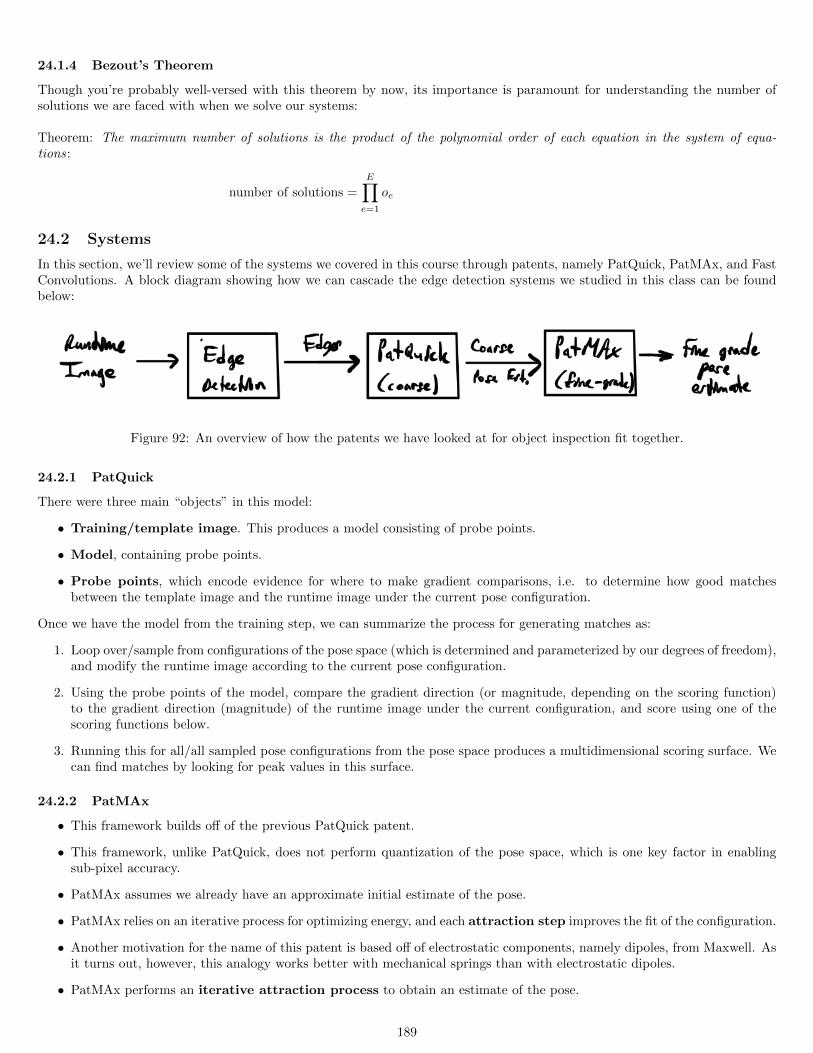
24.1.4 Bezout’s Theorem

Though you’re probably well-versed with this theorem by now, its importance is paramount for understanding the number ofsolutions we are faced with when we solve our systems:

Theorem: The maximum number of solutions is the product of the polynomial order of each equation in the system of equa-tions:

number of solutions =E∏e=1

oe

24.2 Systems

In this section, we’ll review some of the systems we covered in this course through patents, namely PatQuick, PatMAx, and FastConvolutions. A block diagram showing how we can cascade the edge detection systems we studied in this class can be foundbelow:

Figure 92: An overview of how the patents we have looked at for object inspection fit together.

24.2.1 PatQuick

There were three main “objects” in this model:

• Training/template image. This produces a model consisting of probe points.

• Model, containing probe points.

• Probe points, which encode evidence for where to make gradient comparisons, i.e. to determine how good matchesbetween the template image and the runtime image under the current pose configuration.

Once we have the model from the training step, we can summarize the process for generating matches as:

1. Loop over/sample from configurations of the pose space (which is determined and parameterized by our degrees of freedom),and modify the runtime image according to the current pose configuration.

2. Using the probe points of the model, compare the gradient direction (or magnitude, depending on the scoring function)to the gradient direction (magnitude) of the runtime image under the current configuration, and score using one of thescoring functions below.

3. Running this for all/all sampled pose configurations from the pose space produces a multidimensional scoring surface. Wecan find matches by looking for peak values in this surface.

24.2.2 PatMAx

• This framework builds off of the previous PatQuick patent.

• This framework, unlike PatQuick, does not perform quantization of the pose space, which is one key factor in enablingsub-pixel accuracy.

• PatMAx assumes we already have an approximate initial estimate of the pose.

• PatMAx relies on an iterative process for optimizing energy, and each attraction step improves the fit of the configuration.

• Another motivation for the name of this patent is based off of electrostatic components, namely dipoles, from Maxwell. Asit turns out, however, this analogy works better with mechanical springs than with electrostatic dipoles.

• PatMAx performs an iterative attraction process to obtain an estimate of the pose.

189

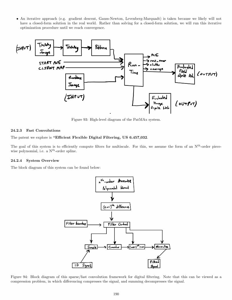
• An iterative approach (e.g. gradient descent, Gauss-Newton, Levenberg-Marquadt) is taken because we likely will nothave a closed-form solution in the real world. Rather than solving for a closed-form solution, we will run this iterativeoptimization procedure until we reach convergence.

Figure 93: High-level diagram of the PatMAx system.

24.2.3 Fast Convolutions

The patent we explore is “Efficient Flexible Digital Filtering, US 6.457,032.

The goal of this system is to efficiently compute filters for multiscale. For this, we assume the form of an Nth-order piece-wise polynomial, i.e. a Nth-order spline.

24.2.4 System Overview

The block diagram of this system can be found below:

Figure 94: Block diagram of this sparse/fast convolution framework for digital filtering. Note that this can be viewed as acompression problem, in which differencing compresses the signal, and summing decompresses the signal.

190

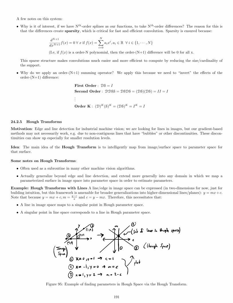
A few notes on this system:

• Why is it of interest, if we have Nth-order splines as our functions, to take Nth-order differences? The reason for this isthat the differences create sparsity, which is critical for fast and efficient convolution. Sparsity is ensured because:

dN+1

dxN+1f(x) = 0 ∀ x if f(x) =

N∑i=0

aixi, ai ∈ R ∀ i ∈ 1, · · · , N

(I.e, if f(x) is a order-N polynomial, then the order-(N+1) difference will be 0 for all x.

This sparse structure makes convolutions much easier and more efficient to compute by reducing the size/cardinality ofthe support.

• Why do we apply an order-(N+1) summing operator? We apply this because we need to “invert” the effects of theorder-(N+1) difference:

First Order : DS = I

Second Order : DDSS = DSDS = (DS)(DS) = II = I

...

Order K : (D)K(S)K = (DS)K = IK = I

24.2.5 Hough Transforms

Motivation: Edge and line detection for industrial machine vision; we are looking for lines in images, but our gradient-basedmethods may not necessarily work, e.g. due to non-contiguous lines that have “bubbles” or other discontinuities. These discon-tinuities can show up especially for smaller resolution levels.

Idea: The main idea of the Hough Transform is to intelligently map from image/surface space to parameter space forthat surface.

Some notes on Hough Transforms:

• Often used as a subroutine in many other machine vision algorithms.

• Actually generalize beyond edge and line detection, and extend more generally into any domain in which we map aparameterized surface in image space into parameter space in order to estimate parameters.

Example: Hough Transforms with Lines A line/edge in image space can be expressed (in two-dimensions for now, just forbuilding intuition, but this framework is amenable for broader generalizations into higher-dimensional lines/planes): y = mx+c.Note that because y = mx+ c,m = y−c

x and c = y −mx. Therefore, this necessitates that:

• A line in image space maps to a singular point in Hough parameter space.

• A singular point in line space corresponds to a line in Hough parameter space.

Figure 95: Example of finding parameters in Hough Space via the Hough Transform.

191

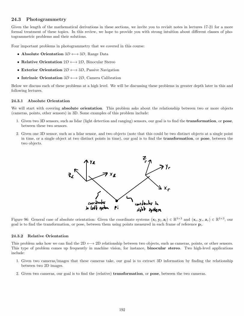
24.3 Photogrammetry

Given the length of the mathematical derivations in these sections, we invite you to revisit notes in lectures 17-21 for a moreformal treatment of these topics. In this review, we hope to provide you with strong intuition about different classes of pho-togrammetric problems and their solutions.

Four important problems in photogrammetry that we covered in this course:

• Absolute Orientation 3D ←→ 3D, Range Data

• Relative Orientation 2D ←→ 2D, Binocular Stereo

• Exterior Orientation 2D ←→ 3D, Passive Navigation

• Intrinsic Orientation 3D ←→ 2D, Camera Calibration

Below we discuss each of these problems at a high level. We will be discussing these problems in greater depth later in this andfollowing lectures.

24.3.1 Absolute Orientation

We will start with covering absolute orientation. This problem asks about the relationship between two or more objects(cameras, points, other sensors) in 3D. Some examples of this problem include:

1. Given two 3D sensors, such as lidar (light detection and ranging) sensors, our goal is to find the transformation, or pose,between these two sensors.

2. Given one 3D sensor, such as a lidar sensor, and two objects (note that this could be two distinct objects at a single pointin time, or a single object at two distinct points in time), our goal is to find the transformation, or pose, between thetwo objects.

Figure 96: General case of absolute orientation: Given the coordinate systems (xl,yl, zl) ∈ R3×3 and (xr,yr, zr) ∈ R3×3, ourgoal is to find the transformation, or pose, between them using points measured in each frame of reference pi.

24.3.2 Relative Orientation

This problem asks how we can find the 2D ←→ 2D relationship between two objects, such as cameras, points, or other sensors.This type of problem comes up frequently in machine vision, for instance, binocular stereo. Two high-level applicationsinclude:

1. Given two cameras/images that these cameras take, our goal is to extract 3D information by finding the relationshipbetween two 2D images.

2. Given two cameras, our goal is to find the (relative) transformation, or pose, between the two cameras.

192

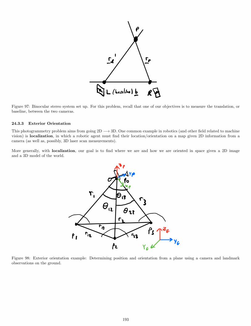
Figure 97: Binocular stereo system set up. For this problem, recall that one of our objectives is to measure the translation, orbaseline, between the two cameras.

24.3.3 Exterior Orientation

This photogrammetry problem aims from going 2D −→ 3D. One common example in robotics (and other field related to machinevision) is localization, in which a robotic agent must find their location/orientation on a map given 2D information from acamera (as well as, possibly, 3D laser scan measurements).

More generally, with localization, our goal is to find where we are and how we are oriented in space given a 2D imageand a 3D model of the world.

Figure 98: Exterior orientation example: Determining position and orientation from a plane using a camera and landmarkobservations on the ground.

193

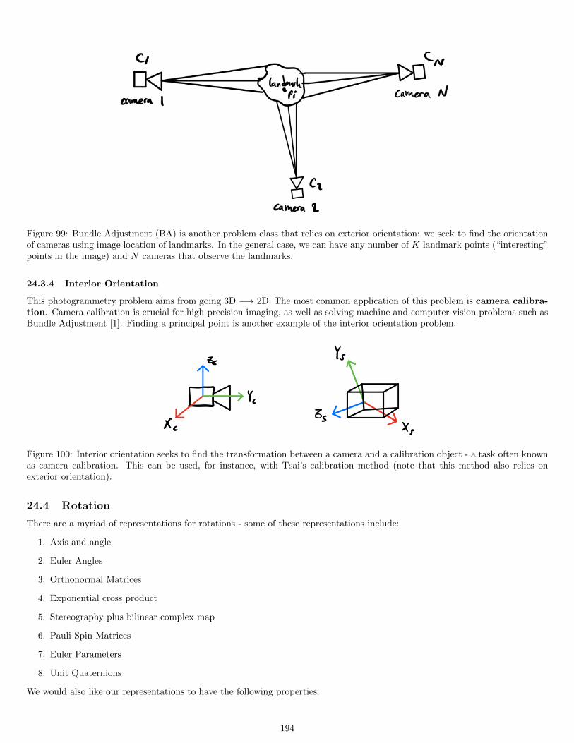
Figure 99: Bundle Adjustment (BA) is another problem class that relies on exterior orientation: we seek to find the orientationof cameras using image location of landmarks. In the general case, we can have any number of K landmark points (“interesting”points in the image) and N cameras that observe the landmarks.

24.3.4 Interior Orientation

This photogrammetry problem aims from going 3D −→ 2D. The most common application of this problem is camera calibra-tion. Camera calibration is crucial for high-precision imaging, as well as solving machine and computer vision problems such asBundle Adjustment [1]. Finding a principal point is another example of the interior orientation problem.

Figure 100: Interior orientation seeks to find the transformation between a camera and a calibration object - a task often knownas camera calibration. This can be used, for instance, with Tsai’s calibration method (note that this method also relies onexterior orientation).

24.4 Rotation

There are a myriad of representations for rotations - some of these representations include:

1. Axis and angle

2. Euler Angles

3. Orthonormal Matrices

4. Exponential cross product

5. Stereography plus bilinear complex map

6. Pauli Spin Matrices

7. Euler Parameters

8. Unit Quaternions

We would also like our representations to have the following properties:

194

• The ability to rotate vectors - or coordinate systems

• The ability to compose rotations

• Intuitive, non-redundant representation - e.g. rotation matrices have 9 entries but only 3 degrees of freedom

• Computational efficiency

• Interpolate orientations

• Averages over range of rotations

• Derivative with respect to rotations - e.g. for optimization and least squares

• Sampling of rotations - uniform and random (e.g. if we do not have access to closed-form solutions)

• Notion of a space of rotations

Let us delve into some of these in a little more depth.

24.4.1 Axis and Angle

This representation is composed of a vector ω and an angle θ, along with the Gibb’s vector that combines these given byω tan

(θ2

), which has magnitude tan

(θ2

), providing the system with an additional degree of freedom that is not afforded by unit

vectors. Therefore, we have our full 3 rotational DOF.

24.4.2 Orthonormal Matrices

We have studied these previously, but these are the matrices that have the following properties:

1. RTR = RRT = I,RT = R−1 (skew-symmetric)

2. det |R| = +1

3. R ∈ SO(3) (see notes on groups above) - being a member of this Special Orthogonal group is contingent on satisfying theproperties above.

24.4.3 Quaternions

In this section, we will discuss another way to represent rotations: quaternions.

24.4.4 Hamilton and Division Algebras

Hamilton’s insight with quaternions is that these quaternions require a “4th dimension for the sole purpose of calculating triples”.Hamilton noted the following insights in order to formalize his quaternion. Therefore, the complex components i, j, k definedhave the following properties:

1. i2 = j2 = k2 = ijk = −1

2. From which follows:

(a) ij = k

(b) jk = i

(c) ki = j

(d) ji = −k(e) kj = −i(f) ik = −j

Note: As you can see from these properties, multiplication of the components of these quaternions is not commutative.

We largely use the 4-vector quaternion, denotedoq = (q,q) ∈ R4.

195

24.4.5 Properties of 4-Vector Quaternions

These properties will be useful for representing vectors and operators such as rotation later:

1. Not commutative:opoq 6= o

qop

2. Associative: (opoq)or =

op(oqor)

3. Conjugate: (p,p)∗ = (p,−p) =⇒ (opoq) =

oq∗op

4. Dot Product: (p,p) · (q,q) = pq + p + q

5. Norm: ||oq||22 =oq · oq

6. Conjugate Multiplication:oqoq∗:

oqoq∗

= (q,q)(q,−q)

= (q2 + q · q, 0)

= (oq · oq)oe

Whereoe

∆= (1, 0), i.e. it is a quaternion with no vector component. Conversely, then, we have:

oq∗oq = (

oqoq)oe.

7. Multiplicative Inverse:oq−1

=oq∗

(oq·oq

(Except foroq = (0,0), which is problematic with other representations anyway.)

We can also look at properties with dot products:

1. (opoq) · (opoq) = (

op · op)(oq · oq)

2. (opoq) · (opor) = (

op · op)(oq · or)

3. (opoq) · or =

op · (oroq

∗)

We can also represent these quaternions as vectors. Note that these quaternions all have zero scalar component.

1.or = (0, r)

2.or∗

= (0,−r)

3.or · os = r · s

4.oros = (−r · s, r× s)

5. (oros) ·

ot =

or · (os

ot) = [r s t] (Triple Products)

6.oror = −(r · r)

oe

Another note: For representing rotations, we will use unit quaternions. We can represent scalars and vectors with:

• Representing scalars: (s,0)

• Representing vectors: (0,v)

24.4.6 Quaternion Rotation Operator

To represent a rotation operator using quaternions, we need a quaternion operation that maps from vectors to vectors. Morespecifically, we need an operation that maps from 4D, the operation in which quaternions reside, to 3D in order to ensure thatwe are in the correct for rotation in 3-space. Therefore, our rotation operator is given:

or′

= R(or) =

oqoroq∗

= (Qor)oq∗

= (QTQ)or

196

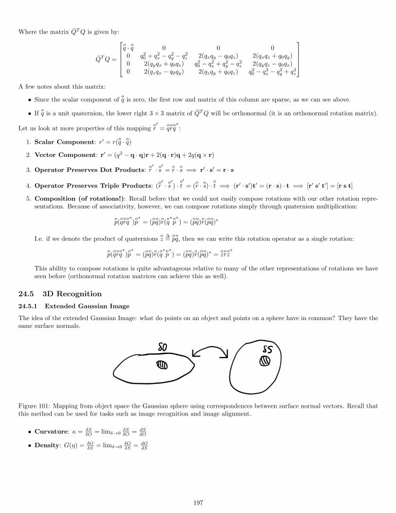
Where the matrix QTQ is given by:

QTQ =

oq · oq 0 0 0

0 q20 + q2

x − q2y − q2

z 2(qxqy − q0qz) 2(qxqz + q0qy)0 2(qyqx + q0qz) q2

0 − q2x + q2

y − q2z 2(qyqz − q0qx)

0 2(qzqx − q0qy) 2(qzqy + q0qz) q20 − q2

x − q2y + q2

z

A few notes about this matrix:

• Since the scalar component ofoq is zero, the first row and matrix of this column are sparse, as we can see above.

• Ifoq is a unit quaternion, the lower right 3× 3 matrix of QTQ will be orthonormal (it is an orthonormal rotation matrix).

Let us look at more properties of this mappingor′

=oqoroq∗:

1. Scalar Component: r′ = r(oq · oq)

2. Vector Component: r′ = (q2 − q · q)r + 2(q · r)q + 2q(q× r)

3. Operator Preserves Dot Products:or′· os′

=or · os =⇒ r′ · s′ = r · s

4. Operator Preserves Triple Products: (or′· os′) ·

ot′

= (or · os) ·

ot =⇒ (r′ · s′)t′ = (r · s) · t =⇒ [r′ s′ t′] = [r s t]

5. Composition (of rotations!): Recall before that we could not easily compose rotations with our other rotation repre-sentations. Because of associativity, however, we can compose rotations simply through quaternion multiplication:

op(oqoroq∗)op∗

= (opoq)or(oq∗op∗) = (

opoq)or(opoq)∗

I.e. if we denote the product of quaternionsoz

∆=

opoq, then we can write this rotation operator as a single rotation:

op(oqoroq∗)op∗

= (opoq)or(oq∗op∗) = (

opoq)or(opoq)∗ =

ozoroz∗

This ability to compose rotations is quite advantageous relative to many of the other representations of rotations we haveseen before (orthonormal rotation matrices can achieve this as well).

24.5 3D Recognition

24.5.1 Extended Gaussian Image

The idea of the extended Gaussian Image: what do points on an object and points on a sphere have in common? They have thesame surface normals.

Figure 101: Mapping from object space the Gaussian sphere using correspondences between surface normal vectors. Recall thatthis method can be used for tasks such as image recognition and image alignment.

• Curvature: κ = δSδO = limδ→0

δSδO = dS

dO

• Density: G(η) = δOδS = limδ→0

δOδS = dO

dS

197

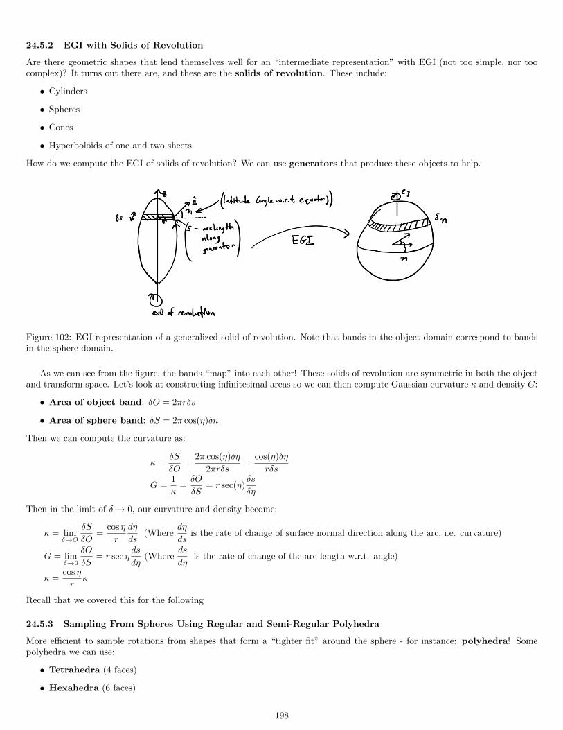
24.5.2 EGI with Solids of Revolution

Are there geometric shapes that lend themselves well for an “intermediate representation” with EGI (not too simple, nor toocomplex)? It turns out there are, and these are the solids of revolution. These include:

• Cylinders

• Spheres

• Cones

• Hyperboloids of one and two sheets

How do we compute the EGI of solids of revolution? We can use generators that produce these objects to help.

Figure 102: EGI representation of a generalized solid of revolution. Note that bands in the object domain correspond to bandsin the sphere domain.

As we can see from the figure, the bands “map” into each other! These solids of revolution are symmetric in both the objectand transform space. Let’s look at constructing infinitesimal areas so we can then compute Gaussian curvature κ and density G:

• Area of object band: δO = 2πrδs

• Area of sphere band: δS = 2π cos(η)δn

Then we can compute the curvature as:

κ =δS

δO=

2π cos(η)δη

2πrδs=

cos(η)δη

rδs

G =1

κ=δO

δS= r sec(η)

δs

δη

Then in the limit of δ → 0, our curvature and density become:

κ = limδ→O

δS

δO=

cos η

r

dη

ds(Where

dη

dsis the rate of change of surface normal direction along the arc, i.e. curvature)

G = limδ→0

δO

δS= r sec η

ds

dη(Where

ds

dηis the rate of change of the arc length w.r.t. angle)

κ =cos η

rκ

Recall that we covered this for the following

24.5.3 Sampling From Spheres Using Regular and Semi-Regular Polyhedra

More efficient to sample rotations from shapes that form a “tighter fit” around the sphere - for instance: polyhedra! Somepolyhedra we can use:

• Tetrahedra (4 faces)

• Hexahedra (6 faces)

198

• Octahedra (8 faces)

• Dodecahedra (12 faces)

• Icosahedra (20 faces)

These polyhedra are also known as the regular solids.

As we did for the cube, we can do the same for polyhedra: to sample from the sphere, we can sample from the polyhedra,and then project onto the point on the sphere that intersects the line from the origin to the sampled point on the polyhedra.From this, we get great circles from the edges of these polyhedra on the sphere when we project.

Fun fact: Soccer balls have 32 faces! More related to geometry: soccer balls are part of a group of semi-regular solids,specifically an icosadodecahedron.

24.5.4 Desired Properties of Dividing Up the Sphere/Tessellations

To build an optimal representation, we need to understand what our desired optimal properties of our tessellations will be:

1. Equal areas of cells/facets

2. Equal shapes of cells/facets

3. “Rounded” shapes of cells/facets

4. Regular pattern

5. Allows for easy “binning”

6. Alignment of rotation

Platonic and Archimedean solids are the representations we will use for these direction histograms.

24.6 References

1. Groups, https://en.wikipedia.org/wiki/Group (mathematics)

199

MIT OpenCourseWarehttps://ocw.mit.edu

6.801 / 6.866 Machine VisionFall 2020

For information about citing these materials or our Terms of Use, visit: https://ocw.mit.edu/terms