7 6 2012 Supplementary material CORRECTED 2genetics.med.harvard.edu/reichlab/Reich_Lab/Publications...Chilote This 10 8 Karitiana HGDP/Kidd 34 13 Toba This 5 4 Chipewyan This 15 15

Table of Contents 1 Note S1 – Data set 2-6 Note S2 – Ancestry estimates 7-8 Note S3 – Ancestry Subtraction to address European and African admixture 9-13 Note S4 – Masking segments of non-Native ancestry 14-16 Note S5 – Correlation of genetic diversity with distance from the Bering Strait 17-18 Note S6 – Documentation of at least three streams of Asian gene flow into America 19-24 Note S7 – Modeling the peopling of America 25-33

Figure S1 – Sampling locations of 17 Siberian populations 34 Figure S2 – Masking of segments of non-Native ancestry 35 Figure S3 – Trees are consistent for masked and unadmixed samples 36 Figure S4 – Admixture Graphs are consistent for masked and unadmixed samples 37 Figure S5 – Heterozygosity and distance from the Bering Strait 38

Table S1 – Summary data for 52 Native American populations 39 Table S2 – Summary data for 17 Siberian populations 40 Table S3 – Individual data for 493 Native American samples 41-47

WWW.NATURE.COM/NATURE | 1

SUPPLEMENTARY INFORMATIONdoi:10.1038/nature

Note S1 Data set (i) Merging data from seven sources We merged seven sets of samples genotyped on Illumina SNP arrays. The number of samples we started with from each population (prior to the final data curation detailed below) is summarized in Table S1.1. Datasets other than the one obtained for this study were pre-filtered by other researchers or in previous rounds of data curation carried out by the authors. Table S1.1: Illumina genotyping data sets that we merged for this analysis Name of dataset N* Comments

“This study” (American and Siberian) 343

Genotyping was performed on Illumina 610-Quad arrays using a combination of genomic and whole genome amplified DNA. The genotyping was performed at the Broad Institute, with the exception of 10 of the 15 Chipewyan samples genotyped at McGill. The initial dataset was pre-filtered to eliminate samples that were genotyped twice, where genotypes were inconsistent with a DNA fingerprint, or where the call rate was <90% (later filters raised this to <95%). We restricted to autosomal SNPs, and removed SNPs with call rate <95% or no physical position.

“Kidd” (American and Siberian) 154 Genotyping was performed on Illumina 650Y arrays.

“MGDP” (Mexican1) 83 Genotyping was performed on Illumina HumanHap550 V3.0 arrays. We

restricted to individuals inferred to be unrelated up to 2nd degree relatives.

“DiRienzo” (Siberian) 63 Genotyping was performed on either Illumina 610-Quad arrays (Nganasan

and Yukaghir) or Illumina 650Y arrays (Naukan and Chukchi)2.

“Willerslev” (Arctic) 142

Genotyping was performed on Illumina 650Y arrays3. We included all samples from ref. 3 except the Na-Dene which did not have permissions appropriate for this study. We then excluded the Yukaghir and Naukan where so many were lost in initial data curation that we removed the whole sample.

“HapMap3” (Worldwide) 799

Genotyping was performed on Illumina 1M and Affymetrix 6.0 arrays4. (The Illumina 1M contains essentially all the SNPs in the Illumina 610-Quad array so we are effectively using the Illumina 1M data from the HapMap3 genotyping.) We removed the Masai (MKK) which had a PCA pattern showing high within-population relatedness.

“CEPH-HGDP” (Worldwide) 907

Genotyping was performed on Illumina 650Y arrays5. We restricted to individuals inferred to be unrelated up to second degree relatives prior to carrying out the additional data curation steps reported below6.

* The sample size quoted here is what we analyzed prior to the final data curation steps reported below. (ii) Curation of Native American samples Our curation excluded samples that genotyped poorly or that had an unusual genetic background relative to other samples from the same population. We first ran the HAPMIX local ancestry inference software (Note S4) to identify segments of the genome in Native Americans and Siberians that may harbor West Eurasian or African ancestry. We then treated the genotypes in these segments as if they were missing data. This “masking” allowed us to better analyze the samples that had some recent European or African ancestry. The estimates of European and African ancestry, and proportion of the genome that was masked, are presented by population in Table S1 for Native Americans and Table S2 for Siberians. The individual ancestry estimates for the Native American samples are presented in Table S3.


SUPPLEMENTARY INFORMATIONRESEARCHdoi:10.1038/nature

We applied the following filters to remove 114 Native Americans samples from the dataset: (1) 18 samples were removed due to a high missing genotype rate

We required that every sample had a genotyping missing data rate of <5%. (2) 32 samples were removed due to a high proportion of West Eurasian or African mixture

We removed samples with <22% of their genomes inferred to have both alleles of entirely Native American ancestry based on the masking analysis of Note S4. The only exception was in Aleutian Islanders where this would have removed all of the samples.

(3) 44 samples were removed due to excess or deficiency of heterozygotes vs. expectation All the Karitiana from the Kidd genotyping had a significant excess of heterozygous genotypes compared with the allele frequency computed in the same samples (violation of Hardy-Weinberg equilibrium). We removed these samples. We also removed a handful of additional samples due to heterozygote excess or deficiency.

(4) 10 samples were removed due to evidence of being at least a 2nd degree relative to others It has already been reported that the Surui sample contained relatives6. For all pairs of individuals in all populations that had evidence for >22% of their genome being shared, we removed one of the pair (in general we chose to remove the one with more missing data). For this purpose, we used SMARTREL, part of the EIGENSOFT package7.

(5) 5 samples were removed due to a noisy local ancestry analysis A total of 5 samples showed a strong mismatch between the ADMIXTURE-based estimate of European and African ancestry proportion (Note S2), and the proportion of the genome that was masked based on HAPMIX local ancestry analysis (Note S4). Visual inspection of the HAPMIX-based local ancestry inference for these 5 showed a noisy baseline ancestry inference compared with other individuals from the same populations, with narrow spikes of potential (but non-confident) non-Native American ancestry, which we interpreted as evidence for poor genotyping. We removed these samples.

(6) 5 samples were removed as PCA outliers relative to others from the same population To identify samples that had unusual genotyping properties relative to other from their own populations we used Principal Component Analysis (PCA) as implemented in EIGENSOFT7. The outlier removal was based on the masked data (Note S4). To ensure that we were not removing samples simply because they had high proportions of their genome masked, we filled in missing data for each SNP based on the mean allele frequency of other samples in the same population (the filled-in data was only used in outlier removal; not for analyses of history). We performed outlier removal restricting to populations with at least 3 samples (outlier removal is impossible with fewer samples), and divided the populations into four groupings to make visual inspection tractable: northern North Americans, Meso-Americans, northern South Americans, and southern South Americans. We iteratively removed samples that were outliers relative to others from the same population on significant eigenvectors, until the samples appeared homogeneous. Aleuts were not included in outlier removal, as masking left almost none of their genome; however, we did remove one Aleut who from local ancestry analysis, appeared to have one chromosome from unadmixed, non-Aleut Native Americans.

After data curation, the number of Native Americans in the merged dataset was 493 (Table S1.2 reports the number of samples removed by population). Importantly, the data curation procedure was based on searching for individuals that were outliers with respect to their own population. Thus, if our curation introduces bias, it would be to make populations more homogeneous; we do not expect it to bias inferences of relationships among populations.



Table S1.2: Record of Native American data curation: filtering from 607 to 493 samples

Population Study Bef

ore

Aft

er


ore

Aft

er


ore

Aft

er

Aleutian Willerslev 9 8 Guarani This 9 6 Piapoco HGDP 7 7 Algonquin This 5 5 Guaymi This 5 5 Pima HGDP/Kidd 46 33 Arara This 2 1 Huetar This 2 1 Purepecha This 1 1 Arhuaco This 6 5 Hulliche This 4 4 Quechua This 41 40 Aymara This 24 23 Inga This 13 9 Surui HGDP/Kidd 30 24 Bribri This 4 4 Jamamadi This 2 1 Tepehuano MGDP 27 25 Cabecar This 32 31 Kaingang This 2 2 Teribe This 3 3 Chane This 2 2 Kaqchikel This 18 13 Ticuna This 6 6 Chilote This 10 8 Karitiana HGDP/Kidd 34 13 Toba This 5 4 Chipewyan This 15 15 Kogi This 6 4 Waunana This 5 3 Chono This 4 4 Maleku This 4 3 Wayuu This 17 11 Chorotega This 1 1 Maya1&2 HGDP/MGDP 56 49 WGInuit Willerslev 8 8 Cree This 5 4 Mixe This 20 17 Wichi This 5 5 Diaguita This 5 5 Mixtec This 5 5 Yaghan This 4 4 EGInuit Willerslev 7 7 Ojibwa This 5 5 Yaqui This 1 1 Embera This 6 5 Palikur This 3 3 Zapotec1&2 This/MGDP 59 43 Guahibo This 13 6 Parakana This 4 1 * The Maya and Zapotec are broken into two subgroups for our analyses in the paper (e.g. Maya1 and Maya2). Table S1.3: Record of Siberian data curation: filtering from 264 to 245 samples


ore

Aft

er


ore

Aft

er

Altaian Willerslev 13 12 Mongolian Willerslev 9 8 Buryat Willerslev 18 17 Naukan DiRienzo 16 16 Chukchi DiRienzo/Willerslev 30 30 Nganasan1&2 DiRienzo/Willerslev 24 22 Dolgan Willerslev 6 4 Selkup Willerslev 9 9 Evenki Willerslev 15 15 Tundra_Nentsi This 4 3 Ket Willerslev 2 2 Tuvinians Willerslev 16 15 Khanty Kidd 39 35 Yakut HGDP/Kidd 40 34 Koryak Willerslev 10 10 Yukaghir Di Rienzo 13 13 * The Nganasan are broken into two subgroups for our analyses in the paper (Nganasan1 and Nganasan2). (iv) Curation of Siberian data We performed a similar analysis in the Siberian populations. This resulted in 17 Siberian populations, after splitting the Nganasan into two based on the two sources of the samples (Willerslev and DiRienzo; the structure was correlated to the sample source, suggesting that these two studies may have sampled different subgroups of the same population). We do not report on the Naukan and Yukaghir populations from the Willerslev dataset in Table S1.3 because so few samples were left from each after outlier removal; we thus removed these populations entirely from the analysis. Table S1.3 summarizes the filtering by population: • 2 samples were removed due to evidence of being at least a 2nd degree relative to others. • 17 samples were removed due to being outliers in PCA relative to their own population. (v) Curation of non-Native American, non-Siberian data We also performed PCA to remove outlier samples from non-Native American and non-Siberian populations. We removed the entire MKK population4 (Masai from Kenya from HapMap3) because of many statistically significant eigenvectors that were difficult to interpret. We also removed 6 other outlier samples. We started from previously filtered



datasets, and hence the number of samples prior to filtering reported in Table S1.1 is sometimes less than that in the papers that originally reported the data. (vi) Merging and splitting of populations Four populations were genotyped both by the Kidd and CEPH-HGDP studies but were known to be from the same original sample collection: Yakut, Karitiana, Surui and Pima. We removed the Kidd Karitiana data because of evidence for heterozygote excess (see above). The two Surui, two Pima, and two Yakut samples were indistinguishable based on PCA, and hence we merged them. The labels we used for the merged data from these populations are:

“Pima” (Kidd Pima and the CEPH-HGDP Pima) “Surui” (Kidd Surui and CEPH-HGDP Surui) “Yakut” (Kidd Yakut and CEPH-HGDP Yakut)

We also merged data from the Chukchi and Quechua because the data we had available from different sources were indistinguishable in PCA:

“Chukchi” (Willerslev Chukchi and DiRienzo Chukchi) “Quechua” (Quechua data from this study and Kidd Quechua)

There were 4 populations for which data were available from two different sources, and for which we kept populations separate based on the source of the samples. We kept the samples separate either because these population samples have been traditionally analyzed separately (for example HapMap3 YRI and HGDP Yoruba), or because we observed differences between the two sources of samples from these populations in PCA (which could reflect genuine population substructure, so we did not want to merge the samples):

Yoruba (“Yoruba” from HGDP; “YRI” from HapMap3) Mongolian (“Mongolian” from Willerslev; “Mongola” from HGDP) Nganasan (“Nganasan1” from Willerslev; “Nganasan2” from Di Rienzo) Zapotec (“Zapotec1” from this study; “Zapotec2” from MGDP)

Finally, PCA showed population substructure in the Maya that did not neatly break down according to the sample source (HGDP or MGDP). This may reflect real substructure: the Maya in MGDP were sampled at multiple sites. We therefore repartitioned as follows:

Maya (“Maya1” from HGDP and MGDP; “Maya2” from MGDP)

(vii) Removal of SNPs with inconsistent or potentially problematic genotyping After merging data for all populations, we curated SNPs as follows: (1) 16 SNPs were removed due to an excess or deficiency of heterozygous genotypes

6 SNPs in the data collected specifically for this study, 6 in the Kidd data, 3 in the Willerslev data, and 1 in the CEPH-HGDP data, showed an extreme excess or deficiency of heterozygotes compared with expectation given the frequency in their populations (their chi-square statistics were visual outliers from the tail).

(2) 16 SNPs were removed due to inconsistency in frequency across data sets For all SNPs, we compared the frequency across populations of similar ancestry. We found 9 SNPs from the genotyping for this study, 6 from HapMap3, and 1 in MGDP, which were consistently more differentiated from the other data sets than expected from the tail of the chi-square distribution, suggesting genotyping error. We removed them.

(viii) Final datasets After curation, we had 2,351 samples and 364,470 autosomal SNPs from 52 Native American, 17 Siberian, and 57 other populations. The average genotyping completeness was



99.88% per sample. The final datasets are listed in Table S1.4. The “unmasked” dataset reflects only the data curation steps described above. The “masked” dataset was obtained based on the results of running HAPMIX to define segments of potential African or West Eurasian ancestry due to admixture in the last few hundred years; SNPs in such segments were then treated as missing (Note S4). All datasets are available on request. Table S1.4: Six datasets generated for this study

Name Samples SNPs Notes Unmasked 2,351 364,470 All data Masked 2,351 364,470 All masked data unmasked.unadmixed 2,021 364,470 Individuals with no evidence of recent admixture unmasked.saqqaq 2,352 68,131 All data* masked.saqqaq 2,352 68,131 All masked data* unmasked.unadmixed.saqqaq 2,021 68,131 Individuals with no evidence of recent admixture*

Note: All files are in the EIGENSOFT “packedancestrymap” format. * These files are merged with genotypes that were previously published based on whole-genome sequencing data from a Saqqaq Paleo-Eskimo individual from Greenland3.

References for Note S1

1 Silva-Zolezzi I, Hidalgo-Miranda A, Estrada-Gil J, Fernandez-Lopez JC, Uribe-Figueroa L, Contreras A, Balam-Ortiz E, del Bosque-Plata L, Velazquez-Fernandez D, Lara C, Goya R, Hernandez-Lemus E, Davila C, Barrientos E, March S, Jimenez-Sanchez G (2009) Analysis of genomic diversity in Mexican Mestizo populations to develop genomic medicine in Mexico. Proc Natl Acad Sci USA 106, 8611-8616.

2 Hancock AM, Witonsky DB, Alkorta-Aranburu G, Beall CM, Gebremedhin A, Sukernik R, Utermann G, Pritchard JK, Coop G, Di Rienzo A (2011) Adaptations to climate-mediated selective pressures in humans. PLoS Genet. 7, e1001375.

3 Rasmussen M. et al. Ancient human genome sequence of an extinct Palaeo-Eskimo. Nature 463, 757-762 (2010).

4 International HapMap 3 Consortium. Integrating common and rare genetic variation in diverse human populations. Nature 467, 52-58 (2010).

5 Li J.Z. et al. Worldwide human relationships inferred from genome-wide patterns of variation. Science 319, 1100-1104 (2008).

6 Rosenberg NA. Standardized subsets of the HGDP-CEPH Human Genome Diversity Cell Line Panel, accounting for atypical and duplicated samples and pairs of close relatives. Ann Hum Genet. 70, 841-847 (2006).

7 Patterson N, Price AL, Reich D (2006) Population structure and eigenanalysis. PLoS Genet. 2, e190.



Note S2 Ancestry estimates

Many of the Native American samples in this study have inherited some European and African genes since 1492. We used the ADMIXTURE clustering software to estimate the proportion of European and African ancestry in each individual1. Following the recommendations of the user manual, prior to running the software we thinned the data until there were no pairs of polymorphisms that had allelic association of r2>0.1, resulting in 88,079 SNPs. We ran ADMIXTURE on the thinned dataset searching for k=2, 3, 4, 5 and 6 clusters. We restricted the analysis to populations that we judged were particularly relevant to learning about Native American population history: • All Native American populations from this study. • 5 Siberian populations chosen to be geographically relatively close to the Bering Strait or to

the Arctic and to cluster in PCA with little evidence of recent mixture (Naukan, Chukchi, Koryak, Nganasan1 and Nganasan2)

• 6 European ancestry populations (French, Italian, Sardinian, Russian, CEU and TSI) • 3 Niger-Kordofanian speaking, sub-Saharan African populations (Yoruba, YRI and LWK) For each cluster number (k=2, 3, 4, 5 and 6), we identified the cluster most correlated to African and European population membership. The assignment to European and African clusters was extremely highly correlated for k=4 and k=5 (Figure S2.1). The only discrepancies between the k=4 and k=5 ancestry estimates are for European ancestry in Nganasan1 and Nganasan2, and thus we did not use the Nganasan in analyses that relied on ADMIXTURE ancestry estimates (in these analyses, we represented Siberians by the Naukan, Chukchi and Koryak only). In contrast, the estimates for k=3 were more weakly correlated to higher cluster numbers (Figure S2.1).

Figure S2.1: ADMIXTURE European and African ancestry estimates compared across k=3-5 clusters. We ran ADMIXTURE on samples from all Native American, 5 Siberian, 6 European and 3 sub-Saharan African populations. We plot the components most strongly correlated with European and African ancestry for k=3, 4 and 5. The inferences for k=4 and k=5 are strongly correlated for both African and European ancestry. The only exceptions are for the Nganasan1 and Nganasan2 (which the k=5 analysis identify as a separate cluster). The validation study in Note S3 suggests the k=4 estimates are strongly correlated to the truth. We focus on the k=4 estimates when we require European and African ancestry estimates.

0%

25%

50%

75%

100%

0% 25% 50% 75% 100%

k=4

k=3

0%

25%

50%

75%

100%

0% 25% 50% 75% 100%

k=5

k=4

0%

25%

50%

75%

100%

0% 25% 50% 75% 100%

k=4

k=3

0%

25%

50%

75%

100%

0% 25% 50% 75% 100%

k=5

k=4

African Component EuropeanComponent

(k=3

)vs.(k=4

)(k=4

)vs.(k=5

)



Based on the high correlation between the k=4 and k=5 ancestry estimates, we hypothesized that the k=4 clustering provides estimates that are highly correlated to European and African ancestry proportion. To test this, we developed a new methodology for estimating a number proportional to an individual’s European ancestry, which we report in Note S3. This analysis confirms that the k=4 ADMIXTURE runs are directly correlated to true ancestry proportion. Based on the k=4 ADMIXTURE runs, we identified an “unadmixed” list of individuals in which the sum of the African and European ancestry estimates for the Native American and Siberian samples is never >0.00025. An advantage of performing analyses on this “unadmixed” dataset is that we do not need to deal with the confounder of recent European and African admixture, and we take advantage of this to establish the robustness of our results. The breakdown of the k=4 ADMIXTURE estimates by sample is given in Table S3 and by population is given in Table S1. The “unadmixed” samples include: • 163 Native American samples from 34 populations (reduced from 493 from 52 populations) • 56 Siberian samples from 3 populations (all the Naukan, Koryak and Chukchi samples) • 333 samples from 7 outgroups (San, Yoruba, YRI, French, CEU, Sardinian and Han)


1 Alexander DH, Novembre J, Lange K (2009) Fast model-based estimation of ancestry in unrelated individuals. Genome Res. 19, 1655-1664.



Note S3 Ancestry Subtraction to address European and African admixture

(i) Motivation There were a number of populations for which we did not have access to unadmixed samples. To learn about the history of such populations, we needed to adjust for the presence of non-Native ancestry. We used three complementary approaches to do this. The concordance of results from all these approaches increases our confidence in the key findings of this study. (1) Restricting to unadmixed samples: We restricted some analyses to 163 Native American

samples (34 populations) without any evidence of recent European or African admixture (Note S2). A limitation, however, is that we could not analyze 16 populations in which all individuals were inferred to have some degree of recent admixture.

(2) Local ancestry masking: We identified genomic segments in each individual that had an

appreciable probability of harboring non-Native American or Siberian ancestry. We then created a “masked” dataset that treated data in these sections as missing (Note S4).

(3) Ancestry Subtraction: We explicitly corrected for the effect of the estimated proportion of

European and African in each sample by adjusting the value of f4-statistics by the amount that is expected from this admixture. This is discussed in what follows.

(ii) Details of Ancestry Subtraction Assume that we have an accurate estimate of African and European ancestry for each sample (whether it is an individual or a pool of individuals). In practice, we used the ADMIXTURE k=4 estimates, because as described below, they appear to be accurate for Native American populations (with the possible exception of Aleuts as we discuss below). We can then define:

a = % African ancestry in a test sample e = % European ancestry in a test sample 1-a-e = % Native ancestry

For many of our analyses, we compute f4 statistics, whose values are affected in a known way by European and African admixture. We thus algebraically correct for the effect of recent European or African admixture on the test statistics, obtaining an “Ancestry Subtracted” statistic that is expected for the sample if it had no recent European or African ancestry. The main context in which we compute f4 statistics is in our implementation of the 4 Population Test, to evaluate whether the allele frequency correlation patterns in the data are consistent with the proposed tree ((Unadmixed, Test),(Outgroup1, Outgroup2)), where the Unadmixed population is a set of Native American samples assumed to derive all of their ancestry from the initial population that peopled America, the Test population is another Native American population, and the two outgroups are Asian populations. An f4 statistic consistent with zero suggests that the Unadmixed and Test populations form a clade with no evidence of ancestry from more recent streams of gene flow from Asia. If the Test population harbors recent European or African ancestry, however, a significant deviation of this statistic from zero would be expected, making it difficult to interpret the results. We thus compute a linear combination of f4 statistics that is expected to equal what we would obtain if we had



access to the Native American ancestors of the Test population without recent European or African admixture:

(S3.1) Intuitively, this statistic is subtracting the contribution to the f4 statistic that is expected from their proportion a of West African-like ancestry (Yoruba), and their proportion e of West Eurasian-like ancestry (French). We then renormalize by 1/(1-a-e) to obtain the statistic that would be expected if the sample was unadmixed. A potential concern is that the African and European ancestry in any real Native American test sample is not likely to be from Yoruba and French exactly; instead, it will be from related populations. However, S1 is still expected to have the value we wish to compute if we choose the outgroups to be East Asians or Siberians. The reason is that genetic differences between Yoruba and the true African ancestors, and French and the true European ancestors, are not expected to be correlated to the frequency differences between two East Asian or Siberian outgroups. Specifically, the allele frequency differences are due to history within Africa or Europe, which is not expected to be correlated to allele frequency differences within East Asia and within Siberia.

(iii) Ancestry Subtraction gives results concordant with those on unadmixed samples To compare the performance of our three approaches to address the confounder of recent European and African admixture, we computed 48 = 8×6 statistics of the form f4(Unadmixed, Test; Han, San). We choose “Unadmixed” to be one of 8 Native American groups from Meso-America southward that have sample sizes of at least two and for which all samples are inferred to be unadmixed by ADMIXTURE k=4 (Chane, Embera, Guahibo, Guaymi, Karitiana, Kogi, Surui and Waunana). We choose “Test” to be one of 8 Native American populations from Meso-America southward with at least two samples that are entirely unadmixed, and that also have at least two samples that have >5% non-Native admixture according to the ADMIXTURE k=4 analysis (Aymara, Cabecar, Pima, Tepehuano, Wayuu and Zapotec1). This allows us to compare results on admixed and unadmixed samples from the same population. If the Test population harbors European or West African admixture that we have not corrected, we expect to see a significant deviation of the statistic from zero. For example, f4(Karitiana, French; Han, San), corresponding to the statistic expected for an entirely European-admixed Native American population, is significant at Z = 45 standard errors from zero, and f4(Karitiana, Yoruba; Han, San), which gives the f4-value we would expect for an entirely West African-admixed Native American population, is significant at Z = 101.

Figure S3.1 shows the scatterplots of Z-scores we obtain without Ancestry Subtraction, with Ancestry Subtraction, and with local ancestry masking (Note S4). The x-axis shows data for the unadmixed samples from each Test population, while the y-axis shows the results for the >5% admixed samples from the same populations. We find that: • Without Ancestry Subtraction there are significant deviations from zero (|Z|>3) (Fig. S3.1A) • With Ancestry Subtraction, there are no residual |Z|-scores >3 (Figure S3.1B) • With local ancestry masking (Note S4), there are again no residual |Z|-scores >3 (Figure

S3.1C), showing that this method also is appropriately correcting for the admixture.



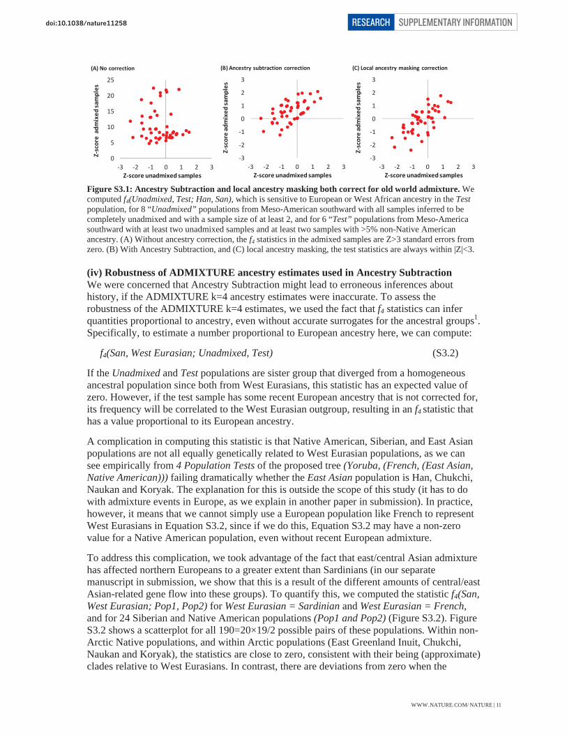
Figure S3.1: Ancestry Subtraction and local ancestry masking both correct for old world admixture. We computed f4(Unadmixed, Test; Han, San), which is sensitive to European or West African ancestry in the Test population, for 8 “Unadmixed” populations from Meso-American southward with all samples inferred to be completely unadmixed and with a sample size of at least 2, and for 6 “Test” populations from Meso-America southward with at least two unadmixed samples and at least two samples with >5% non-Native American ancestry. (A) Without ancestry correction, the f4 statistics in the admixed samples are Z>3 standard errors from zero. (B) With Ancestry Subtraction, and (C) local ancestry masking, the test statistics are always within |Z|<3.

(iv) Robustness of ADMIXTURE ancestry estimates used in Ancestry Subtraction We were concerned that Ancestry Subtraction might lead to erroneous inferences about history, if the ADMIXTURE k=4 ancestry estimates were inaccurate. To assess the robustness of the ADMIXTURE k=4 estimates, we used the fact that f4 statistics can infer quantities proportional to ancestry, even without accurate surrogates for the ancestral groups1. Specifically, to estimate a number proportional to European ancestry here, we can compute: f4(San, West Eurasian; Unadmixed, Test) (S3.2) If the Unadmixed and Test populations are sister group that diverged from a homogeneous ancestral population since both from West Eurasians, this statistic has an expected value of zero. However, if the test sample has some recent European ancestry that is not corrected for, its frequency will be correlated to the West Eurasian outgroup, resulting in an f4 statistic that has a value proportional to its European ancestry.

A complication in computing this statistic is that Native American, Siberian, and East Asian populations are not all equally genetically related to West Eurasian populations, as we can see empirically from 4 Population Tests of the proposed tree (Yoruba, (French, (East Asian, Native American))) failing dramatically whether the East Asian population is Han, Chukchi, Naukan and Koryak. The explanation for this is outside the scope of this study (it has to do with admixture events in Europe, as we explain in another paper in submission). In practice, however, it means that we cannot simply use a European population like French to represent West Eurasians in Equation S3.2, since if we do this, Equation S3.2 may have a non-zero value for a Native American population, even without recent European admixture.

To address this complication, we took advantage of the fact that east/central Asian admixture has affected northern Europeans to a greater extent than Sardinians (in our separate manuscript in submission, we show that this is a result of the different amounts of central/east Asian-related gene flow into these groups). To quantify this, we computed the statistic f4(San, West Eurasian; Pop1, Pop2) for West Eurasian = Sardinian and West Eurasian = French, and for 24 Siberian and Native American populations (Pop1 and Pop2) (Figure S3.2). Figure S3.2 shows a scatterplot for all 190=20×19/2 possible pairs of these populations. Within non-Arctic Native populations, and within Arctic populations (East Greenland Inuit, Chukchi, Naukan and Koryak), the statistics are close to zero, consistent with their being (approximate) clades relative to West Eurasians. In contrast, there are deviations from zero when the

0

5

10

15

20

25

3 2 1 0 1 2 3

Zscoreadmixed

samples

Z score unadmixed samples

(A) No correction

3

2

1

0

1

2

3

3 2 1 0 1 2 3

Zscoreadmixed

samples


(B) Ancestry subtraction correction

3

2

1

0

1

2

3

3 2 1 0 1 2 3

Zscoreadmixed

samples


(C) Local ancestry masking correction



comparisons are between non-Arctic Native and Arctic populations, with non-Arctic Native populations showing consistent evidence of being genetically closer to West Eurasians.

Figure S3.2: French and Sardinians have different proportions of Asian admixture, letting us learn a correction factor. We compute f4(San, West Eurasian; Pop1, Pop2) for 20 Native American and Siberian populations with at least 3 samples inferred to be unadmixed. The statistics are divided into comparisons of two non-Arctic Native populations or two arctic populations (where the statistics are usually close to zero), and comparisons of non-arctic and arctic populations where they often deviate strongly. The statistics are highly correlated, with the magnitude for West Eurasian = Sardinian 0.75 of West Eurasian = French.

The observation of non-zero statistics when one of the Native populations is Arctic and the other is a more southern Native American population is a complication, since we would like Ancestry Subtraction to work not just for southern Native American populations, but also for northern North Americans who have inherited genetic material from multiple streams of Asian migration. However, the fact that Sardinian statistics are smaller than the French statistics by a constant factor (0.75), allows us to adjust for this difference by regression. Specifically, we can compute a linear combination S2 of the French and Sardinian statistics that subtracts out the effect of central/east Asian gene flow into West Eurasians and has an expected value of zero. This can be viewed as the expected value of f4(San, West Eurasian; Pop1, Pop2), for a hypothetical West Eurasian population that does not have any history of admixture from Asians (because we have subtracted away that ancestry): (S3.3) In practice, we had to also deal with a further complication of African admixture in some populations, so we computed a slightly more complicated statistic that subtracts out the expected effect of this ancestry:

(S3.4) We compared S3 to the ADMIXTURE k=4 estimate for diverse Native American populations. For the reference “Pop1” in S3, we used a pool of unadmixed Native American, Koryak, Naukan and Chukchi samples (Note S2), deleting any individuals that overlapped the Test sample. For the Test, we analyzed populations with at least three samples). Figure S3.3 shows that the inferences are highly correlated (r2=0.97), providing confidence in the ADMIXTURE k=4 estimates. However, two populations are notable in that their ADMIXTURE estimates are |Z|>3 standard errors from the fitted regression line:

• The Chilote have an ADMIXTURE k=4 estimate of 37.7% ancestry vs. an extrapolated 44.0 ± 1.6% from our method (nominally Z=3.9 standard errors different).

• The Aleuts have an ADMIXTURE k=4 estimate of 64.8% European ancestry vs. an extrapolated 56.7 ± 2.2% from our method (nominally Z=3.7 standard errors). We

y = 0.7526xR² = 0.9568

0.0015

0.001

0.0005

1E 17

0.0005

0.001

0.0015

0.0015 0.001 0.0005 1E 17 0.0005 0.001 0.0015

f4(San,Sardinian;Po

p1,P

op2)

f4(San, French; Pop1, Pop2)

NatAm NatAmNatAm ArcticArctic ArcticAllLinear (All)



hypothesize that this difference is due to over- or under-correcting for European ancestry in the Aleuts due to inaccurate ADMIXTURE k=4 ancestry estimates. Thus, we cannot confirm our finding that the Aleuts share ancestry with the Inuit based on Ancestry Subtraction. However, the robustness of the inferences from local ancestry masking in other cases makes us think the inference based on masking is likely to be correct in this case too.

Figure S3.3: Correlation between k=4 ADMIXTURE estimates of European ancestry and the S3statistic. We restrict to populations with at least 3 samples to reduce noise in the visualization. The high correlation suggests that both methodologies are producing meaningful inferences about ancestry. The strongest discrepancies are seen in the Chilote and Aleuts; we are cautious about using Ancestry Subtraction for these populations.


1 Reich, D., Thangaraj, K., Patterson, N., Price, A.L. & Singh, L. Reconstructing Indian population history. Nature 461, 489-494 (2009).

y = 0.01643xR² = 0.96678

0.0020

0.0000

0.0020

0.0040

0.0060

0.0080

0.0100

0.0120

0% 10% 20% 30% 40% 50% 60%S 3prop

ortio

naltoEu

rope

anan

cestry

ADMIXTURE k=4 European ancestry estimate



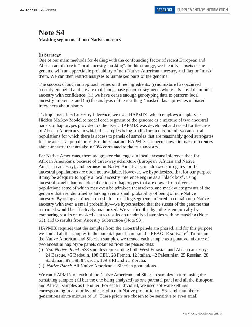
Note S4 Masking segments of non-Native ancestry (i) Strategy One of our main methods for dealing with the confounding factor of recent European and African admixture is “local ancestry masking”. In this strategy, we identify subsets of the genome with an appreciable probability of non-Native American ancestry, and flag or “mask” them. We can then restrict analyses to unmasked parts of the genome.

The success of such an approach relies on three ingredients: (i) admixture has occurred recently enough that there are multi-megabase genomic segments where it is possible to infer ancestry with confidence; (ii) we have dense enough genotyping data to perform local ancestry inference, and (iii) the analysis of the resulting “masked data” provides unbiased inferences about history. To implement local ancestry inference, we used HAPMIX, which employs a haplotype Hidden Markov Model to model each segment of the genome as a mixture of two ancestral panels of haplotypes provided by the user1. HAPMIX was developed and tested for the case of African Americans, in which the samples being studied are a mixture of two ancestral populations for which there is access to panels of samples that are reasonably good surrogates for the ancestral populations. For this situation, HAPMIX has been shown to make inferences about ancestry that are about 99% correlated to the true ancestry1. For Native Americans, there are greater challenges in local ancestry inference than for African Americans, because of three-way admixture (European, African and Native American ancestry), and because for Native Americans, unadmixed surrogates for the ancestral populations are often not available. However, we hypothesized that for our purpose it may be adequate to apply a local ancestry inference engine as a “black box”, using ancestral panels that include collections of haplotypes that are drawn from diverse populations some of which may even be admixed themselves, and mask out segments of the genome that are identified as having even a small probability of being of non-Native ancestry. By using a stringent threshold—masking segments inferred to contain non-Native ancestry with even a small probability—we hypothesized that the subset of the genome that remained would be effectively unadmixed. We verified this hypothesis empirically by comparing results on masked data to results on unadmixed samples with no masking (Note S2), and to results from Ancestry Subtraction (Note S3).

HAPMIX requires that the samples from the ancestral panels are phased, and for this purpose we pooled all the samples in the parental panels and ran the BEAGLE software2. To run on the Native American and Siberian samples, we treated each sample as a putative mixture of two ancestral haplotype panels obtained from the phased data: (i) Non-Native Panel: 538 samples representing both West Eurasian and African ancestry:

24 Basque, 45 Bedouin, 108 CEU, 28 French, 12 Italian, 42 Palestinian, 25 Russian, 28 Sardinian, 88 TSI, 8 Tuscan, 109 YRI and 21 Yoruba.

(ii) Native Panel: All Native American + Siberian populations. We ran HAPMIX on each of the Native American and Siberian samples in turn, using the remaining samples (all but the one being analyzed) as one parental panel and all the European and African samples as the other. For each individual, we used software settings corresponding to a prior hypothesis of a non-Native proportion of 5%, and a number of generations since mixture of 10. These priors are chosen to be sensitive to even small



proportions of non-Native admixture. However, previous simulations have shown that HAPMIX priors have minimal effect on ancestry inference for admixture in the last handful of generations1, the scenario relevant here. At each locus, HAPMIX infers the probability that an individual has 0 (p0), 1 (p1) and 2 (p2) alleles of non-Native ancestry. Figure S2 shows examples. We defined the expected number of non-Native alleles at any locus is E = p1 + 2p2. We then masked any section of the genome with E>0.01, choosing a stringent threshold because we wished to remove any segment that had even a small chance of harboring non-Native ancestry.

Figure S4.1: Comparison of the estimated proportion of non-Native ancestry to the proportion of the genome masked. On the x-axis we plot the ADMIXTURE k=4 estimate of the percent European and African ancestry, and on the y-axis the percent of the genome masked. If masking is perfect, we expect y = 2x-x2 = 1-(1-x)2 of the genome to be masked, and this expectation is shown by the smooth curve. There is a strong correlation between expected and observed. In practice, we mask 2.1% more of the genome than expected on average, reflecting our aggressive masking.

To assess if masking is performing as expected, Figure S4.1 plots the ADMIXTURE k=4 estimate for each sample against the masked proportion of the genome3. The expected proportion y of the genome that is masked given that a fraction x of their alleles are of non-Native American ancestry is y = 2x-x2 = 1-(1-x)2 (assuming Hardy-Weinberg equilibrium), and is a good match to the observed data with the exception that the masked portion of the genome is on average 2.1% in excess of the theoretical expectation overall. Some excess is expected given the aggressive threshold we use to remove segments that are of potentially non-Native American ancestry, so we do not find this excess to be surprising. There are also a few outlier samples in Figure S4.1 for which more of the genome is masked than would be expected from the genome-wide ancestry estimate. Detailed examination of the strongest outliers, who have >11% more of the genome masked than expected from theory, shows that they were almost all cases where the method never inferred more than one non-Native chromosome (Figure S4.1). This is the pattern expected for a first generation mixture of an admixed individual and an unadmixed individual—an individual who is not in Hardy-Weinberg equilibrium—leading to a larger proportion of their genome being masked than would be expected from an individual whose parents are both equally admixed. The fact that these individuals are outliers is expected, and restricting to subsets of the genome that are unmasked for these individuals should not result in any bias in historical inferences, since the segments that remain after the masking are expected to be entirely Native American in origin.

(ii) No evidence that masking biases our inferences about history A concern is that there are biases in the segments of Native American genomes that we are masking. Because we are running HAPMIX in a “black box” mode for a scenario in which it has never been rigorously tested (three way mixture and using complex mixtures of

0%

20%

40%

60%

80%

100%

0% 20% 40% 60% 80% 100%

Percen

tofthe

geno

memasked

Estimated non Native American ancestry from ADMIXTURE

Actual percentmasking

Expected percentmasking



populations some of which are poor surrogates for the true ancestral populations as haplotype panels), it may be producing inaccurate estimates of ancestry probability at some segments of the genome, causing us to include in our dataset genuine segments of non-Native American ancestry despite the stringent thresholds that we apply to retain only the most confidently inferred segments. We explored whether the thresholds we used for local ancestry masking are substantially affecting our inferences. The main analyses in the paper are based on E<0.01 and using all Siberian and Native American samples as the ancestral Native panel. However, we also explored the effect of masking using more permissive thresholds (E<0.1), and performing the local ancestry inference using a Native panel that consisted only of Native Americans. The percentage of the genome masked was similar in all four analyses that we performed (15.6%-17.0%; Table S4.1). For the analyses reported in the main paper, we decided to use the threshold of E<0.01, and also to use both Native Americans and Siberians for the Native ancestral panel, because: (a) we wished to be as confident as possible that we are analyzing Native American segments for studying history; (b) we only lose a small amount of data by discarding segments with even a small probability of non-Native ancestry; and (c) visually, ancestry inferences in Arctic populations were crisper when we included Siberians in the ancestral panel (presumably because we used a more comprehensive ancestral haplotype panel). Table S4.1: Percentage of the genome masked when using different masking strategies

Masking threshold Ancestral Native panel % genome masked in Native Americans E<0.1 Native Americans only 15.6% E<0.01 Native Americans only 17.0% E<0.1 Native Americans and Siberians 15.3% E<0.01 Native Americans and Siberians 16.6%

As a second approach to testing whether our inferences are robust to the masking procedure, throughout the paper we also compared key results obtained with the masked data to those from either (a) removing samples that are inferred to have any admixture at all (Note S2), or (b) explicitly correcting for non-Native American ancestry (Ancestry Subtraction; Note S3). The consistency of inferences made from masked data with those made from the other approaches is also evident when we build Neighbor Joining trees (Figure S3) and when we build an Admixture Graph relating populations (Figure S4). References for Note S4

1 Price AL, Tandon A, Patterson N, Barnes KC, Rafaels N, Ruczinski I, Beaty TH, Mathias R, Reich D, Myers S (2009) Sensitive detection of chromosomal segments of distinct ancestry in admixed populations. PLoS Genet. 5, e1000519.

2 Browning SR, Browning BL (2007) Rapid and accurate haplotype phasing and missing data inference for whole genome association studies using localized haplotype clustering. Am J Hum Genet 81, 1084-1097.

3 Alexander DH, Novembre J, Lange K (2009) Fast model-based estimation of ancestry in unrelated individuals. Genome Res. 19, 1655-1664



Note S5 Correlation of genetic diversity with distance from the Bering Strait

We estimated heterozygosity by using the masked data (so as to eliminate the confounder of recent European and African admixture). We restricted analysis to populations with at least five samples to reduce sampling variation. To obtain a heterozygosity estimate for each population, we used the masked dataset. The heterozygosity estimate was obtained by dividing the number of heterozygous genotypes over all individuals from the population, by the number of genotypes that were present in the dataset (Table S1). Geographic distance from the Bering Strait was computed using great arc routes from an Anadyr start point at 64.8N 177.8E, with the location of each population specified by the coordinates in Table S1 (where more than one sample was available for a population, we used a position mid-way between the two sampling locations and averaged population heterozygosity over the samples). We computed a Pearson correlation coefficient between the mean observed population heterozygosity and the distance from Beringia, for all 32 Native American populations with a sample size of at least 5. We evaluated statistical significance with a t-distribution transformation (using the R-package1). The data we used for these analyses are reported in Table S5.1. To evaluate the effects of coasts as facilitators of migration, we also computed “effective”, or “least-cost path” distances2. Compared to the geographic great arc distances, effective distances incorporate the effects of one or several landscape components. They are computed as least-cost paths on the basis of a spatial cost map that incorporates these components. The effective distance is computed as the sum of costs (“cost distance”) along the paths. Because the relative cost of landscape components is arbitrary, we tested a range of combinations. For example, a ratio of 1:10 coastline/land means that it is ten times more costly to go through land than through coastline. In addition to simple great arc distances, we used the following coastline/inland cost combinations: 1:2, 1:5, 1:10, 1:20, 1:30, 1:40, 1:50, 1:100, 1:200, 1:300, 1:400 and 1:500. When all populations are considered, we observe a negative correlation between heterozygosity and distance from the Bering Strait (Figure S5, r=-0.48, P=0.007). This correlation increases when considering effective distances, reaching a maximum at a coastline/inland cost combination of 1:5 (Figure S5, r= -0.51, P= 0.004). When we exclude from this analysis the four northern North American populations (Aleuts, East Greenland Inuit, West Greenland Inuit and Chipewyan) that have unambiguous evidence of additional streams of genetic input from Asia (Note S6) the negative correlation remains (r=-0.34, P=0.091) becoming stronger when effective distances are considered, again with a maximum at a coastline/inland ratio of 1:5 (Figure S5 r= -0.39, P= 0.049). An exception to the pattern of decreasing heterozygosity with distance from Beringia is populations from the Isthmo-Colombian area which mostly have low diversity relative to the expectation based on their distance from the Bering Strait. As we document in the main text, these populations derived most of their ancestry from eastern South America and the current geographic location of some of them (north of the Panama isthmus) reflects complex population movements and admixtures in the region. Further exclusion from this analysis of the Isthmo-Colombian populations results in a correlation of heterozygosity with distance



from the Bering Strait of r=-0.50 (P=0.022). This increases with effective distances reaching a maximum at a coastline/inland ratio of 1:10 (Figure S5: r= -0.70, P= 0.0004).

Table S5.1: Heterozygosity and distance from the Bering Strait Population N Heterozygosity Great Arc Distance (m) Aleutian* 8 0.260 1,788,963 Chipewyan* 15 0.251 2,998,535 Ojibwa 5 0.249 5,184,797 West Greenland Inuit* 8 0.247 5,408,260 Pima 33 0.259 5,432,128 Algonquin 5 0.237 5,619,796 East Greenland Inuit* 7 0.237 5,786,292 Tepehuano 25 0.246 6,205,875 Mixtec 5 0.247 7,105,459 Maya 37 0.250 7,138,397 Mixe 17 0.242 7,140,781 Zapotec 22 0.248 7,181,122 Kaqchikel 13 0.250 7,538,473 Cabecar* 31 0.221 8,397,297 Guaymi* 5 0.214 8,588,582 Arhuaco* 5 0.208 8,746,097 Wayuu 11 0.234 8,788,814 Embera* 5 0.221 9,025,514 Guahibo 6 0.230 9,481,686 Inga 9 0.230 9,576,373 Piapoco 7 0.235 9,833,731 Ticuna1 6 0.225 10,391,952 Karitiana 13 0.221 11,346,772 Quechua1 40 0.244 11,484,968 Surui 24 0.206 11,493,384 Aymara 23 0.244 11,941,135 Wichi 5 0.220 12,486,648 Guarani 6 0.246 12,739,695 Diaguita 5 0.243 12,960,201 Chilote 8 0.238 13,914,216

* These populations were removed in sub-analyses.


1 R Development Core Team. R: A language and environment for statistical computing. (Vienna, Austria, 2010). 2 Ray N (2005) PATHMATRIX: a geographical information system tool to compute effective distances among

samples. Molecular Ecology Notes 5, 177-180.



Note S6 Documentation of at least three streams of Asian gene flow into America (i) Motivation A key question is whether Native Americans today descend from a single ancient gene flow event from Asia, or alternatively harbor ancestry from multiple streams of Asian gene flow. To address this, we began by performing 4 Population Tests1 using the statistic f4(Southern Native American, Test Population; Outgroup1, Outgroup2) where the statistic is defined as:

(S6.1)

Here, ai, bi, ci and di are the variant allele frequencies at SNP i in populations A, B, C and D respectively. The statistic is proportional to the correlation in allele frequencies differences (Southern Native American - Test Population) and (Outgroup1 - Outgroup2) over all SNPs. It has an expected value of zero if the Southern Native American and Test Population are sister groups that descend from a homogeneous ancestral population. By using a Block Jackknife standard error, we obtain an approximately normally distributed Z-score that serves a formal test for whether the 4 populations are consistent with the unrooted tree. (ii) Most Native Americans descend from a homogeneous Asian ancestral population We computed the f4 statistic using all 52 Native American populations in turn as the Test Population. For the pair of Asian outgroups, we used all possible pairs of 10 populations: Han and 9 Siberian populations, restricting to Siberian populations with at least ten samples that are not known to have any history of back-migration from Arctic Native Americans (this criterion excluded the Naukan Eskimo who are culturally related to the Greenland Inuit, and the Chukchi some of whom are known to have admixed with the Yupik-speaking Naukan). For each of 52 Native American populations, we computed up to 135 = 45×3 f4 statistics. There were 45=9×8/2 possible pairs of Asian outgroups and we tested all. We also tested three Southern Native American reference samples: (i) 13 Karitiana (unadmixed South Americans), (ii) 5 Guaymi (unadmixed Meso-Americans), or (iii) 158 individuals from an “Unadmixed Pool”. The “Unadmixed Pool” was obtained by pooling all individuals from Mexico southward inferred by ADMIXTURE k=4 to be unadmixed (Note S2). The f4 statistics obtained using the “Unadmixed Pool” were highly correlated to those in the Karitiana and Guaymi, but with smaller standard errors owing to larger sample size and reduction of population-specific genetic drift.

There were two minor complications: (i) When the Karitiana and Guaymi were the Test Population, we could not use them as the

Southern Native American population. We thus only computed 90 = 45×2 f4 test statistics for testing these two populations for compatibility with a simple tree.

(ii) When the Unadmixed Pool contained individuals that were also in the Test Population, we removed the samples in the Test Population from the pool so as not to use the same samples twice. This slightly reduced the sample size of the Unadmixed Pool.

Table S1 presents the maximum |Z| score for a deviation from zero obtained for these f4 statistics, for each of 52 Native American Test Populations. We used a threshold for significance of |Z|>4.5, corresponding to P<0.05 after correcting for 7,020 hypotheses tested ((52 populations) × (45 statistics) × (3 Southern Native American populations)). There were 4 populations that crossed this threshold, all from northern North America (nearly identical



results are obtained for the Ancestry Subtracted data and unadmixed samples; Table S1). Their maximum |Z| scores are given in Table S6.1. The same test for the Saqqaq Greenland sample—which we performed for the approximately one sixth of SNPs for which we have data for the Saqqaq individual—shows that they too must have ancestry from later Asian gene flow (maximum |Z|=5.9; Table S6.1). Table S6.1: Populations with different relationship to Asians vs. southern Native Americans

Max. |Z| for different Southern Nat. Am. P-value from Bonferroni P-value for the

Population Karitiana (36 tests)

Guaymi (36 tests)

Unadmixed Pool (36 tests)

correction for 135 tests in max. |Z|-score analysis

Hotelling T-test

W.G. Inuit 16.5 14.6 14.2 <10-9 <10-9

E.G. Inuit 16.4 14.6 14.6 <10-9 <10-9 Chipewyan 6.0 4.6 4.8 2×10-7 <10-9 Saqqaq 5.9 5.2 5.3 5×10-7 2×10-9 Aleutian 4.9 4.6 4.9 3×10-4 9×10-5

Note: This table lists all populations with both a Hotelling T-test P<0.005 and maximum |Z|-score of 4.5. All analyses are performed on masked data, but results are consistent in the unmasked data and in unadmixed samples (Table S1).

Figure S6.1: Qualitative evidence of 3 different patterns of relatedness to Asians among Native Americans. We plot f4 statistics for all possible pairs of northern Native American populations with the strongest evidence of a distinct relationship to Asians compared with more southern Native Americans. Two groupings of populations harbor significantly different historical relationships with a panel of 10 Asian outgroups. Within groups, f4 statistics are highly correlated, whereas across groups they are significantly different: the P-value in each panel is from Table 1: the Hotelling T-test for whether the vectors of f4 statistics are consistent with being scalar multiples of each other. The dashed line is added to highlight the difference in within-group and across-group comparison.

(iii) New method for distinguishing the number of distinct migrations into America For each of the Test Populations from North America with a significantly different pattern of relatedness to the panel of 10 Asian populations from what is seen in Southern Native Americans, we plotted the values of 45 f4 statistics of the form f4(Southern Native American, Test Population; Outgroup1, Outgroup2), using the Unadmixed Pool as Southern Native Americans. Figure S6.1 plots the 45 f4 statistics for all possible pairs of five populations (the four Native American groups and the Saqqaq Greenland sample) in the masked data. We observe two groupings of populations that differ qualitatively from each other as well as from more southern Native Americans. One grouping includes Greenland Inuits (and possibly Aleuts), and a second grouping includes the Chipewyan (and possibly the Saqqaq).

Saqqaq

E. Green. Inuit AleutianW. Green. Inuit

.64

Aleutian

E. Green. Inuit

Aleutian

Chipewyan

Chipewyan

W.Green

Inuit

W. Green. Inuit

W.G

reen.InuitAleutian

Chipewyan

Chipewyan

Saqqaq

.57

.02

6x10 6

.41

.006

2x10 6

.03

.17 .29



To place these qualitative observations on a solid statistical footing, we generalized the analysis of f4 statistics by developing new methodology. If two Native American populations derive all their non-First American ancestry from the same ancestral stream of Asian gene flow, their vectors of f4 statistics are expected to be scalar multiples of each other, and we developed a formal statistical test for whether this is the case. Given a phylogeny and a set of four populations P, Q, R, S we define F4 as the expected value of the f4 statistic, that is: F4(P,Q,R, S) = E[f4(P,Q;R,S)] = E[(p q)(r s)] (S6.2)

Here, p, q, r, s are alleles of P, Q, R, S. We code an allele as 1 if it is a variant allele and 0 if it is a reference allele (the opposite convention gives the same f4-statistics). We now choose a Southern Native American group P (say Karitiana or a pool of populations from Meso-American southward) and an Outgroup1 population R (say Han) in Asia. Thus, we can write a two-dimensional matrix of F4 values with rows corresponding to the number of Native American populations (Q) that are tested, and columns corresponding to the number of Asian populations (S) that are tested: X(Q, S) = F4(Karitiana,Q;Han,S) (S6.3)

Theorem Let r be the rank of X, and n the number of independent gene flows into the Americas. Then r + 1 n (S6.4)

The proof is straightforward. We use induction on n. If n = 1, then r = 0, or equivalently X = 0. This is our familiar f4-based 4 Population Test. A single gene flow from Asia initially can only increase the rank by 1. Subsequent drift in the Americas does not change X except to add noise (since allele frequency changes due to drift are uncorrelated to the allele frequency differences between the Asian groups R and S). Admixture of populations within the Americas only has the effect of adding new rows to the matrix that are linear combinations of the pre-existing rows, and thus does not increase the rank. This completes the proof. To apply this result, we fix populations P and R, choose m Native American populations to represent Q, and choose n Asian populations to represent S. We then have an m × n matrix Y: Y(Q, S) = f4(P,Q;R,S) (S6.5)

Our matrix X is the expected value of our data matrix Y, given a specific demographic history relating the analyzed populations. Using a weighted Block Jackknife2, we can estimate a covariance matrix V for Y. V has dimension mn × mn. To score for rank k we can fit Y(B,D) = A × B where A is m × k, and B is k × n. The log-likelihood is: (S6.6)

where

C = Y - AB (S6.7)

This likelihood function allows us to apply a Likelihood Ratio Test (LRT). We can post-multiply A by any non-singular k × k matrix M, and pre-multiply B by M. It follows that our



rank k model for Y has k(m+n k) degrees of freedom. Testing rank k+1 versus rank k is then a standard LRT, leading to a 2 statistic under the null hypothesis that the F4 matrix has rank k. For the important case m = 1, in which we wish to test if X is 0 (or equivalently that the rank of X is 0), our statistic is a Hotelling T2 statistic3. We refine our test, not using the 2 distribution, but an F-statistic. In our weighted Block Jackknife we use 5 centimorgan blocks, with the weight i for block i being the number of SNPs in block i. The F-test requires as a parameter the number of ‘independent’ blocks d. We use an ansatz: (S6.8)

and take T2 to be Fn,d-n distributed under the null. Fortunately d is large (several hundred) and F is approximately n

2, so the exact value of d is not very important here. To test larger values of k we simply use the asymptotic 2 distribution. (iv) At least three streams of gene flow from Asia are needed to explain the dataWe used the new statistical method described in section (iii) to identify 43 southern Native American populations that are consistent with deriving all their ancestry from the same initial migration within the limits of our resolution. To identify this set of populations, we began by using the Brazilian Karitiana as a “seed” Southern Native American population (P in Equation S6.4), and considered each of the other 52 Native American populations in turn as the Test Population (Q in Equation S6.4). A total of 41 populations gave non-significant test statistics for deriving from the same ancestral gene flow event as the Karitiana (P>0.1), and we pooled them. We then retested the remaining 14 populations now using the pool to represent Southern Native Americans, and identified 2 additional populations with non-significant statistics (including Karitiana). The final pool of 43 is a subset of the 48 identified by maximum |Z|-score analysis. Table S1 gives the P-values from a formal test for whether each of the 52 Native American populations in the dataset has evidence for deriving ancestry from a distinct stream of Asian gene flow from the 43 Southern Native American populations (when the Test Population is one of the 43 Southern Native Americans, we construct a new pool of 42 populations excluding the Test Population). This identifies four populations with Hotelling T-test P-values <0.00009, which are the same as the four populations that emerge as significant form the maximum |Z|-score analysis (Table S6.1). The only other formally significant signal is in the Maya2 (P=0.0007), but the maximum Z-score analysis is not significant here (P=0.22), and the closely related Maya1 show no signal (P=0.50). Given that after correcting for testing 52 hypotheses this observation is only weakly significant (P=0.04) we view this result as uncompelling. In what follows, we therefore focus on studying the four populations that give consistent signals of ancestry from later streams of Asian gene flow in both the maximum |Z|-score and Hotelling T-test analyses. The same analysis applied to the Saqqaq Greenland sample shows that it, too, derives ancestry from a later stream of Asian gene flow (P=2×10-9), consistent with the original analysis of data from this sample4, and so we add this population as a fifth group in what follows. For all 10 = 5×4/2 possible pairs of the 5 populations in Table S6.1, we evaluated whether the data are consistent with the hypothesis that the later Asian genetic material in both of the populations derives from the same source; that is, we tested the null hypothesis that the rank of the matrix is k=1. To represent Southern Native American populations in this analysis, we



used the pool of 43 Native American populations from Meso-America southward consistent with having ancestry entirely from First Americans (Table S1). The P-values are given both in Table 1 and in the bottom right of the panels in Figure S6.1. This identifies two groupings of populations consistent with the qualitative patterns in Figure S6.1: Eskimo-Aleut speakers (East / West Greenland Inuit and probably Aleuts), and the Chipewyan and possibly the Saqqaq. Within groupings, P-values are always non-significant or marginally significant, whereas across groupings, they are significant. Based on these results, we pooled populations for further testing: Southern (43 populations; 406 samples), Eskimo-Aleut (East Greenland Inuit, West Greenland Inuit, and Aleuts; 23 samples), and Chipewyan (15 samples). We also considered the Saqqaq as a potentially fourth group. Application of the methods of (iii) to our data result in three main findings: (1) At least three streams of gene flow from Asia to America occurred. Specifically, when we

simultaneously analyze Southern Native Americans, Eskimo-Aleut speakers, and Chipewyan, we reject a single stream of later Asian gene flow (P=0.011; Table S6.2).

(2) The Chipewyan have a different pattern of relatedness to Asians than the Eskimo-Aleut. (3) The Saqqaq are consistent with having their Asian ancestry from the same stream of later

gene flow as the Chipewyan (P=0.29; Table S6.2). Table S6.2: Analysis of the masked data indicate at least 3 streams of gene flow with Asia

Population groupings simultaneously tested No. of pop. groupings simultaneously tested

P-value for this many streams of gene flow being sufficient to

explain the observed patterns 1 2 3

Southern / Eskimo-Aleut 2 <10-9 . . Southern / Chipewyan 2 <10-9 . . Southern / Saqqaq 2 2×10-9 . . Southern / Eskimo-Aleut / Chipewyan 3 <10-9 .011 . Southern / Eskimo-Aleut / Saqqaq 3 <10-9 2×10-6 . Southern / Chipewyan / Saqqaq 3 <10-9 0.29 . Southern / Eskimo-Aleut / Chipewyan / Saqqaq 4 <10-9 8×10-6 0.27

Note: For analyses involving the Saqqaq, we have about six-fold fewer SNPs. This table is somewhat redundant to Table 1. Table S6.3: Analysis restricted to unadmixed samples confirms 3 streams of gene flow

Population groupings simultaneously tested No. of pop. groupings simultaneously tested

P-value for this many streams of gene flow being sufficient to

explain the observed patterns 1 2 3

Southern / East Greenland Inuit 2 <10-9 . . Southern / Chipewyan 2 1×10-7 . . Southern / Saqqaq 2 <10-9 . . Southern / East Greenland Inuit / Chipewyan 3 <10-9 .49 . Southern / East Greenland Inuit / Saqqaq 3 <10-9 4×10-6 . Southern / Chipewyan / Saqqaq 3 <10-9 0.32 . Southern / East Greenland Inuit / Chipewyan / 4 <10-9 2×10-6 0.56

Note: This is the same as Table S6.2 except we restrict to unadmixed samples: a pool of 30 “Southern” populations identified by the same iterative process as described for the masked dataset, 3 East Greenland Inuit, 2 Chipewyan and 1 Saqqaq. To assess if our inference about the minimum number of streams of gene flow between Asia and America is robust to local ancestry masking, we repeated the analyses using the subset of samples that we inferred in Note S2 are unadmixed. Results are consistent, although due to the smaller sample sizes for the Chipewyan and Eskimo-Aleut speakers, we no longer have



power to distinguish the Asian ancestries in these groups (P=0.49; Table S6.3). Our data continue to be consistent with no more than 3 streams of gene flow when we include the Saqqaq (Table S6.3). (v) A genetic link between the Saqqaq and Na-Dene speakersIn the Saqqaq genome paper, the authors co-analyzed the data they collected with data from diverse present-day populations from Siberia and the America. Based on the patterns that they observed in Principal Component Analysis, they argued that the Saqqaq have ancestry from a different stream of gene flow into America than Eskimo-Aleut speakers, Na-Dene speakers, and Southern Native Americans4. However, this is not a formal test: the failure to cluster together in the first few principal components does not necessarily imply that populations are unrelated; just that they do not share much genetic drift on their common ancestral lineage. Our conclusions differ: • We confirm that the Saqqaq derive from a different stream of Asian gene from southern

Native Americans (P=2×10-9 rejecting 1 stream), and also that they derive from a different stream of Asian gene flow from Eskimo-Aleut speakers (P=2×10-6 rejecting the hypothesis that Southern Native Americans, Eskimo-Aleut and Saqqaq derive from 2 migrations) (Table S6).

• We cannot confirm that Saqqaq derive from a stream of Asian gene flow distinct from that which led to Na-Dene speakers like the Chipewyan. When we test the hypothesis that the Saqqaq and Chipewyan descend from the same second stream, we cannot reject it (P=0.29), and we also cannot reject the hypothesis that Southern Native Americans, Eskimo-Aleut, Chipewyan and Saqqaq derive from just 3 streams of Asian gene flow (P=0.27). In Note S7, we confirm these inferences by presenting a formal model showing that the Saqqaq and Chipewyan can be fit as deriving from the same stream of Asian ancestry.

Our finding that the Saqqaq harbor ancestry that is deeply shared with the Chipewyan raises the possibility of a historical link between the ancestors of the Saqqaq and Na-Dene speakers, that is, that they descend from a common stream of Asian gene flow into America. However, an alternative that we cannot rule out is that there were two streams of Asian gene flow into America from related Asian populations whose ancestries we cannot distinguish. An important direction for future research will be to study additional Na-Dene speaking populations and Siberian populations. This will provide more power to test if the Asian ancestry in these two groups is different. It will also allow more general statements about whether the ancestry in the Chipewyan (related to the Saqqaq) is shared across Na-Dene speakers. We note that the authors of the Saqqaq genome paper were unable to share with us the data from the Na-Dene speaking population they studied, and so we could not evaluate whether that sample harbors the same signal of Saqqaq-related ancestry as the Chipewyan.



2 Busing, F.M.T.A., Meijer, E. & van der Leeden, R. Delete-m jackknife for unequal m. Statistics and Computing 9, 3-8 (1999).

3 Mardia K.V., Kent J.T. & Bibby, J.M. Multivariate Analysis. Academic Press (1979). 4 Rasmussen M. et al. Ancient human genome sequence of an extinct Palaeo-Eskimo. Nature 463, 757-762

(2010).



Note S7 Modeling the peopling of America (i) Admixture Graphs Trees present an oversimplified view of population relationships, as they assume all groups descend from a common ancestor by a series of bifurcations without subsequent admixture. As a tool for learning about population mixture events, we used Admixture Graphs (AGs)1. AGs are generalizations of trees that accommodate the possibility of unidirectional admixture between branches (edges) of the tree. Thus, AGs allow us to propose models of population relationships that are more complex than a simple tree, and to test whether they are consistent with the data. While many AGs in principle might be consistent with a dataset, our goal is to identify a parsimonious AG that does not predict any pattern of allele frequency correlation across populations (as measured by f-statistics) that is grossly inconsistent with the data. This distinguishes an AG from the Neighbor Joining tree of Figure 1C, which is grossly inconsistent in that it predicts patterns of allele frequency correlations among populations that are discrepant with the data as reflected in highly significant 4 Population Tests.

By itself, an AG just specifies the topology of population relationships (like a tree). However, once a topology is specified, one can infer the mixture proportions for each admixture event, as well as the amount of genetic drift that occurred historically on each lineage (variation in allele frequencies due to sampling variation in the context of limited effective population size) that best fit the data. An AG in which these quantities are specified determines the values of all possible “f-statistics” measuring the correlation in allele frequencies among two (f2), three (f3), and four (f4) populations1. We can then compare these to the observed values (which have a standard error from a Block Jackknife) to assess whether there is any evidence for a poor fit. (The 4 Population Test is a special case of Admixture Graph model testing, since it tests whether particular f4 statistics have the value of zero expected if those four populations are related by a simple tree.) A valuable feature of AGs is that they are robust to ascertainment bias of SNPs (how the SNPs were chosen for inclusion in the study), making them useful for inferring tree topologies even using data from SNP microarrays1. To assess whether a proposed AG is consistent with a dataset, we have implemented software (ADMIXTUREGRAPH) that begins with a proposed topology, and finds the combination of branch lengths and admixture proportions that best fit the data. We measure the fit to data by testing the match between all possible f-statistics predicted by the model and the data: for a given set of N populations, this is (N(N-1)/2 f2 statistics, 3N(N-1)(N-2)/6 f3 statistics, and 3N(N-1)(N-2)(N-3)/24 f4 statistics. A complication is that the f-statistics are correlated (for example, all the f3 and f4 statistics can be written as linear combinations of f2 statistics), and thus it is difficult to know how many hypotheses we are effectively testing. To deal with this, we compute a 2 statistic measuring the difference between all observed and predicted f-statistics taking into account the covariance structure (and using an error covariance from a Block Jackknife). This serves as a score that allows us to climb to a best fitting model.

At present, we do not know how to calculate how many degrees of freedom are effectively being used in the model (given the correlation among all the f-statistics), and hence we do not believe that our AG technology supports a formal P-value for a goodness-of-fit test. At best, we have a nominal P-value. This is similar to problems that affect almost all model-fitting in population genetics, where “Composite Likelihoods” are used that do not support formal



goodness-of-fit tests because of correlations among the statistics used to constrain the model. However, we can nevertheless make statements about consistency of the data and model: (a) For a fixed complexity of Admixture Graph (fixed number of populations and admixture

events), we have a formal test for which graph topologies are most likely. We use this in Figure 3 to produce the coloring of the edges, which shows all the AGs that are consistent with the proposed topology within a 2 differential of 3.84 (P<0.05 by a 2 test with one degree of freedom). The idea is that while we do know how many degrees of freedom are relevant to the computation of our 2statistic, for a fixed number of parameters, we can compare the fits of AGs to the data, because they all have the same number of degrees of freedom. By taking the difference between the AG with the smallest (best fitting) 2

value, and other AGs with the same number of parameters, we have a formal test of the relative goodness of fit given a fixed number of parameters.

(b) Another way to make meaningful statements about whether a fitted AG is consistent with data is to test whether it predicts f-statistics among populations that are never too extreme. In practice, we view any AG that produces an f-statistic more than |Z|>4 standard errors from expectation as a graph that we wish to avoid. (For AGs with a sufficient number of populations, |Z|>4 is expected by chance even if the graph is a correct representation of history, and so this may be too stringent a criterion.) We also count the number of f-statistics that are |Z|>3 standard errors from expectation, and minimize this too.

(ii) The relationship of First Americans to speakers of Eskimo-Aleut languages We first used the Admixture Graph methodology to search for models that could relate Eskimo-Aleut speakers to the group of Native American populations stretching from Canada all the way to southern Chile who are consistent with deriving from the same ancestral population, a group whose ancestry we call “First American”. Figure S7.1 shows how each Eskimo-Aleut speaking populations in turn can be fit into an AG with populations of entirely First American ancestry (we used Algonquin to represent Canadians, Zapotec1 to represent Meso-Americans, and Karitiana to represent South Americans). All the AGs are consistent with the data in the sense that none of the predicted f-statistics are |Z|>3 standard errors from expectation. The P-values from our approximate 2 statistic are shown in the upper left corner of each panel, and are always non-significant. Eskimo-Aleut speakers have >50% First American ancestry Inuit and Aleutian islanders can be fit to allele frequency correlation patterns if we treat them as admixtures of a First American lineage that branched off within the radiation of Native Americans (below Algonquin), and an East Asian lineage that is a sister group to Han (Figure S7.1). AGs without an admixture event in the history of these populations are poor fits (see the 4 Population Tests in the previous section). Strikingly, the inferred First American ancestral proportions are always at least 50%. Thus, the data suggest that after arriving in the Americas, the Asian ancestors of the Inuits and the Aleuts admixed with resident Native Americans. The mixed populations then gave rise to groups with these ancestries today. To assess whether alternative topologies are equally good fits to the data as the one shown in Figure S7.1, we used the East Greenland Inuit as a representative Eskimo-Aleut speaking population, and tried all possible AGs with 0 or 1 admixture events relating the populations in the top left panel of Figure S7.1. Only two AGs are consistent with our data, both specifying admixture in the history of the East Greenland Inuit. The best fitting AG is shown. The 2 statistic increases by 1.8 for the next-best fitting AG (the Algonquin branching off more recently than the First American admixture into the Inuit, an AG we discuss further below). All other AGs have a 2 for the fit at least 32 higher and so are not plausible fits.



Figure S7.1: Inuits, Aleuts, Chukchi and Naukan are well modeled as harboring First American ancestry. All these populations can be modeled as mixtures of First Americans and an Asian lineage related to Han. The AGs show drifts in parts per 1000 in units proportional to FST, and mixture proportions on dotted lines. The AGs are consistent with the data in that none produces |Z|-scores more than 3 standard errors from 0 whether. We report P-values in the top left (masked data).

Speakers of Algonquin languages carry the deepest First American lineages The AGs that are fit in Figure S7.1 hypothesize that the deepest First American leading is that leading to the Algonquin, not the one admixing into Eskimo-Aleut speakers. This is counterintuitive, as one might expect the deepest Native American branches to be in the most northern parts of America (found in admixed form in Eskimo-Aleut speakers). The fit of this AG to the data is only slightly poorer than the model shown in Figure S7.1, as reflecting in the fact that the two models have a 2 statistic difference of only 1.8, which is not significant. To explore this further, we refit the AG in the top left of Figure S7.1, now replacing the Algonquin with another population speaking a related language, the Ojibwa. The 2 statistic for the model shown is 6.3 less the alternative model in which the Ojibwa are not the deepest First American lineage (P=0.012). This suggests that the Figure S7.1 topology is a better fit to the data, and that Algonquin-speakers do in fact carry a deeper First American lineage. Movement of First American genes into Asia, mediated by Eskimo-Aleut speakers We next built a larger AG that analyzes multiple Eskimo-Aleut speaking populations together. Figure S7.2 shows that we obtain an excellent fit for a model in which the Naukan (Siberian Eskimo), both Greenland Inuit populations, and the Aleuts are in the same AG (to

P=.33 P=.34

P=.24 P=.23 P=.25



help in visualization, blue is used to indicate First American ancestry, and red to indicate Eskimo-Aleut related ancestry). A history that fits this model is: (1) First American ancestors migrated

to America >15,000 years ago (2) Eskimo-Aleut ancestors migrated

more recently, mixing with First Americans they encountered. This mixed population was ancestral to present-day Eskimo-Aleut speakers.

(3) Movement of Eskimo-Aleut speakers to Asia accounts for the First American ancestry in the Naukan. The First American ancestry in the Chukchi could reflect contacts between the Naukan and Chukchi2 (a subset of the samples are from Aion Island, who have some ancestry from Yupik-speaking Naukan). Alternatively, it could reflect a separate history of gene exchange between Chukchi and Native Americans. Circum-Arctic gene flow in both directions between Siberia and America has been supported by various data, including single locus studies, and our study confirms this.

(iii) A model of history that relates the Chipewyan and Saqqaq to First Americans We next identified a model of history that fits the data for the Saqqaq and Chipewyan, who were suggested by Note S6 to have some related ancestry. Following the analyses involving Eskimo-Aleut speakers, we identified a simple AG for each of the populations separately, and then fit them along with Zapotec1, Karitiana, Algonquin, and both Han and Yoruba as outgroups. We then evaluated the robustness of the fits and explored more complex AGs. The ancestors of both Chipewyan and Saqqaq admixed with First Americans We first tried fitting both Chipewyan and Saqqaq in a simple way into the AG, without admixture. In both cases, there is no good fit. For the Saqqaq, the nominal significance of the fit is P=0.006 and there is an outlier f-statistic at Z=3.1. For the Chipewyan, the nominal significance of the best fitting AG without an admixture event is P<10-9. We next tried fitting both populations with a single admixture event, and found good fits for both Chipewyan (P=0.33) and Saqqaq (P=0.44) (for both, there are no f-statistics with values

Figure S7.2: An AG that fits all Eskimo-Aleut speaking Native American populations along with the Naukan Siberian Eskimo. There are no f-statistics |Z|>3 standard errors from expectation, and the nominal P-value is 0.77. The model specifies that Eskimo-Aleut speakers (red) descend from an admixture event of First American (blue) and Asian lineages. This occurred after the initial migration of Eskimo-Aleut Asian ancestors to the Americas, after which the ancestors of Aleuts separated from the Inuit. A back-migration of Eskimo-Aleuts would have then led to the Naukan, who admixed with Asians they encountered (~9% of their ancestry). We tried all alternative AGs, and found that the only others consistent with the data corresponded to the change of the recent Asian admixture in Naukan coming off in a slightly different place in relation to Han (lineages labeled as drifts “9” and “15”).



more than 3 standard errors from expectation). For the Chipewyan, there are several AGs that are topologically similar to the one in the left panel of Figure S7.3 that are equally good fits to within the limits of our resolution. For the Saqqaq, the AG shown in Figure S7.3 is the only one that fits the data at all (the next-best fitting AG has a 2 statistic that is 6.9 higher). These analyses suggest that after arriving in America, the Asian ancestors of both populations admixed with the First American populations already there (an estimated 89% for the Chipewyan speakers, and 14% for the Saqqaq). The finding of admixture with First Americans is parallel to what we infer occurred in the history of Eskimo-Aleut speakers.

Figure S7.3: Admixture Graphs that fit Chipewyan and Saqqaq. We show the best fitting graphs for Chipewyan and Saqqaq (nominal P-values at top left, and in parentheses when computed on unadmixed samples). The coloring is added to highlight the streams of ancestry leading to First Americans (blue), and Saqqaq and Chipewyan (green) Chipewyan and Saqqaq admixed with a deeper First American lineage than Eskimo-Aleuts A notable difference between the Eskimo-Aleuts on the one hand, and the Chipewyan and Saqqaq on the other, is the source of their First American ancestry. Comparing Figure S7.1-3, the First American ancestry in Eskimo-Aleut speakers is inferred to come from a more derived lineage than that seen as Algonquin speakers, whereas the Chipewyan and Saqqaq are consistent with having their First American ancestry from the deep Algonquin lineage. This supports the view, suggested also by Note S6, that the stream of later Asian gene flow that contributed ancestry to Eskimo-Aleut speakers, followed a different historical course than the one(s) that contributed to the Chipewyan and Saqqaq. It also is consistent with the suggestion in Note S6 that the Chipewyan and Saqqaq may have shared Asian ancestry. A model of shared Asian ancestry in the Chipewyan and Saqqaq that fits the data We finally constructed an AG that fit the data for both the Chipewyan and Saqqaq as deriving from the same Asian lineage, with subsequent admixture in different proportions from a deep First American lineage related to that in present-day Algonquin speakers (rightmost panel of Figure S7.3). There is no evidence for a poor fit (P=0.40, with no outlier f-statistics |Z|>3 standard errors from expectation). The next best fitting AG with the same complexity is a significantly worse fit (the 2 statistic is 9.2 higher). Thus, our data continue to be consistent with the model that the Chipewyan and Saqqaq harbor a distinct and possibly shared streams of later Asian ancestry compared with First Americans and Eskimo-Aleut speakers.

(iv)A model that fits data from First Americans, Eskimo-Aleut speakers, & Chipewyan We identified an AG that fits the data for selected populations from representatives of all the groupings of populations simultaneously, which we show in Figure 2. This AG is a fit to the

P=.33 P=.40 P=.40



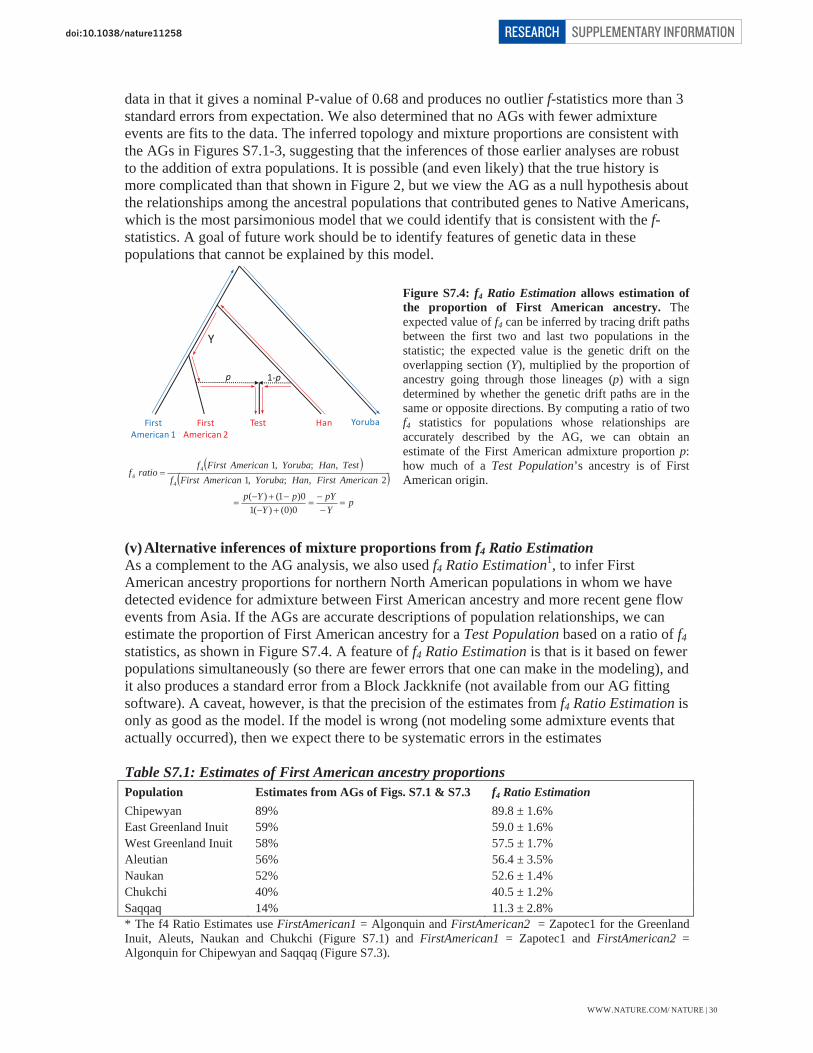
data in that it gives a nominal P-value of 0.68 and produces no outlier f-statistics more than 3 standard errors from expectation. We also determined that no AGs with fewer admixture events are fits to the data. The inferred topology and mixture proportions are consistent with the AGs in Figures S7.1-3, suggesting that the inferences of those earlier analyses are robust to the addition of extra populations. It is possible (and even likely) that the true history is more complicated than that shown in Figure 2, but we view the AG as a null hypothesis about the relationships among the ancestral populations that contributed genes to Native Americans, which is the most parsimonious model that we could identify that is consistent with the f-statistics. A goal of future work should be to identify features of genetic data in these populations that cannot be explained by this model.

Figure S7.4: f4 Ratio Estimation allows estimation of the proportion of First American ancestry. The expected value of f4 can be inferred by tracing drift paths between the first two and last two populations in the statistic; the expected value is the genetic drift on the overlapping section (Y), multiplied by the proportion of ancestry going through those lineages (p) with a sign determined by whether the genetic drift paths are in the same or opposite directions. By computing a ratio of two f4 statistics for populations whose relationships are accurately described by the AG, we can obtain an estimate of the First American admixture proportion p: how much of a Test Population’s ancestry is of First American origin.

(v) Alternative inferences of mixture proportions from f4 Ratio EstimationAs a complement to the AG analysis, we also used f4 Ratio Estimation1, to infer First American ancestry proportions for northern North American populations in whom we have detected evidence for admixture between First American ancestry and more recent gene flow events from Asia. If the AGs are accurate descriptions of population relationships, we can estimate the proportion of First American ancestry for a Test Population based on a ratio of f4 statistics, as shown in Figure S7.4. A feature of f4 Ratio Estimation is that is it based on fewer populations simultaneously (so there are fewer errors that one can make in the modeling), and it also produces a standard error from a Block Jackknife (not available from our AG fitting software). A caveat, however, is that the precision of the estimates from f4 Ratio Estimation is only as good as the model. If the model is wrong (not modeling some admixture events that actually occurred), then we expect there to be systematic errors in the estimates Table S7.1: Estimates of First American ancestry proportions Population Estimates from AGs of Figs. S7.1 & S7.3 f4 Ratio EstimationChipewyan 89% 89.8 ± 1.6% East Greenland Inuit 59% 59.0 ± 1.6% West Greenland Inuit 58% 57.5 ± 1.7% Aleutian 56% 56.4 ± 3.5% Naukan 52% 52.6 ± 1.4% Chukchi 40% 40.5 ± 1.2% Saqqaq 14% 11.3 ± 2.8% * The f4 Ratio Estimates use FirstAmerican1 = Algonquin and FirstAmerican2 = Zapotec1 for the Greenland Inuit, Aleuts, Naukan and Chukchi (Figure S7.1) and FirstAmerican1 = Zapotec1 and FirstAmerican2 = Algonquin for Chipewyan and Saqqaq (Figure S7.3).

Y

p 1 p

YorubaFirstAmerican 1

FirstAmerican 2

Test Han

pYpY

YpYp

AmericanFirstHanYorubaAmericanFirstfTestHanYorubaAmericanFirstf

ratiof

0)0()(10)1()(

2,;,1,;,1

4

44



(vi) A model that fits the data for 16 First American and 2 Outgroup populations To build an AG fitting data for 16 Native American populations (Figure 3), we restricted to populations that had samples sizes of at least 2 and are consistent with descending from a homogeneous ancestral population without subsequent gene flow from Asians (that is, they are of entirely First American ancestry). We included all populations with entirely First American ancestry among the populations we attempted to fit into the AG. We used Yoruba (West Africans) and Han (Chinese) as outgroups. Our process of building the AG was ad hoc, involving manually adding populations until we were no longer able to add additional ones without producing many f-statistics |Z|>3 standard errors from expectation, or without producing a large incremental increase of the difference between the 2 statistic and estimated number of degrees of freedom. An important area for future research will be to develop more principled algorithms for building AGs. Nevertheless, we believe that the AG in Figure 3 is useful in providing a hypothesis for how these populations are related that is not grossly inconsistent with the data. The allele frequency correlation patterns in a dataset with this number of SNPs provide strong constraints on possible relationships, and finding any model that relates such a large number of populations provides a useful starting point for further research into population relationships. Of the 16 Native American populations in the AG, 13 can be fit to a simple tree with no evidence of admixture. An additional 3 can only be included in the AG through admixture (Cabecar, Inga and Guarani). The resulting AG (Figure 3) provides a reasonable fit in the sense that there is only one f-statistic |Z|>3 standard errors from zero (|Z|=3.2, not surprising given that we evaluated 11,781 statistics), and the nominal significance of the entire fit is P=0.53. The AG fitting also produces estimates of genetic drift on each lineage (in units scaled to be comparable to 1000×FST), and mixture proportions, which are shown in Figure 3. Standard errors in f-statistic values are ~0.001. Thus, short branches (e.g. of length 1 = 1000×0.001) are not reliably inferred; the data are consistent with trifurcations at such nodes. To assess the robustness of our inferences to local ancestry masking, we repeated the AG analysis on a subset of 10 Native American populations that contained at least one sample without any European or African ancestry (this excluded Algonquin, Hulliche, Chilote, Inga, Kaingang and Mixtec). Figure S4A shows the fitted AG on the masked data and Figure S4B for the subset of samples from these populations that are completely unadmixed. For the analysis on the masked data, only two of 2,211 f-statistics are |Z|>3 from expectation (both |Z|<3.2), and the overall P-value for the fit is P=0.37. For the analysis that restricts to unadmixed samples, there are no f-statistics |Z|>3 standard errors from expectation, and the overall fit is P=0.42. The consistency with the topology of Figure 3 provides confidence that our inferences of population relationships from masked data are not artifactual. The Admixture Graph analysis in Figure 3 suggests that the Inga, Guarani, and Cabecar can be modeled as resulting from simple admixture events. We discuss each case in turn. Inga In the tree of Figure 1C, the Inga cluster with their geographic neighbors rather than with their linguistic neighbors, suggesting a priori that a mixture event is plausible. To test if the Inga can be fit into the tree without admixture, we created a new AG in which the Inga were removed, and then reinserted them at each edge of the AG without admixture. The best fitting AG in which the Inga are not admixed is one in which they are in a clade with the Guahibo (consistent with the AG in which the inferred largest mixture component is from a group



related to the Guahibo; Figure 3). However, this AG is clearly inconsistent with the genetic data: there are 35 f-statistics that are |Z|>3 greater than expectation, with the largest being |Z|=4.8. When we model the Inga as an admixed population, we do obtain a reasonable fit as shown in Figure 3. We also explored all other AGs that model the Inga as deriving from a single admixture event, and found only one that is statistically consistent (the 2 statistic is 2.5 larger) and this AG has a similar topology. We conclude that the Inga descend from a mixture of lineages related to western South American Andean-speaking groups (like Quechua and Aymara) and Amazonian South American Equatorial-Tucanoan-speaking groups (like Guahibo), consistent with their speaking and Andean language but living on the eastern side of the Andes close to Amazonian populations. Guarani The Guarani (like the Inga) cluster in Figure 1C with their geographic neighbors rather than with their linguistic neighbors, suggesting a priori that they might be admixed. Consistent with this, the Guarani can be well-fit into the AG is as an admixture of their immediate geographic neighbors and an Equatorial-Tucanoan speaking group (whose language group they share) (Figure 3). We also tried fitting the Guarani without admixture. The single best fitting AG places the Guarani as a clade with the ancestral population of the Wichi. For this AG, there are 9 f-statistics that are more than |Z|>3 standard errors from expectation with the largest at |Z|=3.8; moreover, the 2 statistic for the best model without admixture is 22.8 higher than the best model with admixture. Thus, a history of admixture is strongly supported by the data. We tried all possible insertion points of the two admixing lineages leading to the Guarani, and found only two AGs with 2 statistics within 3.8 of the best model. In all of these AGs, one admixing lineage is a clade with the Wichi. The other lineage is always in the Guahibo-Surui-Palikur clade, but its exact placement within the clade is uncertain. Chibchan-speaking populations The third inferred admixture event is in the Cabecar, a Chibchan-speaking population from north of the Panama isthmus. Figure 3 shows red and blue coloring to indicate the edges that are consistent with being the insertion points of the two lineages ancestral to the Cabecar and that have 2 statistics within 3.84 of the best fitting AG. When we instead fit the data for the Cabecar without admixture, the fits are poorer (Table S7.2). The difference between the nominal 2 statistic and the number of degrees of freedom jumps from -2 (AG of Figure 3) to 22, and the number of |Z|-scores greater than 3 jumps from 1 to 14. Thus, the data appear to strongly support admixture in the history of the Cabecar. To assess the generality of the inference of admixture of North and South American lineages in the history of Chibchan-speakers, we measured the fit of the AG model to the genetic data for the 10 Chibchan-Paezan speaking populations in the largely Chibchan-Paezan speaking clade of Figure 1C (the only populations that do not speak Chibchan-Paezan languages in this clade are the Wayuu and Chorotega and we excluded them). We proceeded as follows: (a) We removed the Cabecar from the AG of Figure 3, and then reinserted each of the

Chibchan-clade populations as a mixture of two lineages from the resulting AG. (Usually the admixing lineages are similar in their inferred insertion points to the Cabecar.)

(b) Each of the 10 populations in turn is treated as unadmixed and we find the best fit model.

Table S7.2 shows the results. All of the 10 populations fit the data far better with a model of an admixture of North and South American lineages than with a model of no admixture: the difference between the nominal 2 statistic and the estimated number of degrees of freedom always jumps by at least 14 (Huetar) to as high as 25 (Waunana) between the best fitting



model without admixture and the one with admixture. Without admixture, 9 of the 10 populations have at least nine |Z|-scores >3; in contrast, with admixture, there are at most 5 |Z|-scores >3. (The worst fit is the Huetar.) Table S7.2: Admixture Graphs fitted to populations in the mostly Chibchan-Paezan clade, showing models with North/South American mixture are more likely than models without

Best fit as an unadmixedpopulation

Best fit as an admixture of North and South American lineages

Decrease in ( 2 – no. degrees of freedom) when an admixture

event is allowed 2 - d.o.f No. |Z|

stats >3 Max.

|Z| 2 - d.o.f No. |Z|

stats >3 Max. |Z|

Guaymi 13 27 3.8 -6 1 3.2 19 Cabecar 22 14 4.0 -3 1 3.2 25 Embera 22 17 3.7 -1 1 3.2 23 Maleku 19 7 3.6 4 2 3.2 16 Teribe 26 22 3.9 5 3 3.2 21 Waunana 30 10 3.4 5 2 3.2 25 Kogi 26 33 3.8 9 4 3.3 17 Bribri 33 56 4.5 11 2 3.2 22 Arhuaco 39 69 4.1 20 1 3.3 20 Huetar 57 29 4.1 43 5 3.3 14

Motivated by these results, we attempted to fit a substantial proportion of Chibchan-speaking populations into an AG in which there was a single admixture event ancestral to South and North American Chibchan speakers. We were able to obtain a reasonable fit for an AG with three populations (Cabecar, Maleku and Kogi). However, we had difficulty in fitting a larger number. We hypothesize that this reflects additional admixture events or isolation-by-distance processes involving populations related to other groups in the AG of Figure 3. These analyses produce two key inferences: (1) A model of admixture of North and South American lineages is needed to fit the data for

almost all Chibchan-speaking populations. (2) All Chibchan-speakers today likely inherit most of their genetic material from ancestors

in South America, as the lineage that the AG fits as contributing most of the ancestry of Chibchan speakers falls within the radiation of South Americans (after the branching of Andean-speaking South Americans like Quechua; indicated by red shading in Figure 3).

One hypothesis that could explain these observations is that the North American Chibchan speakers inherited all their North American-related ancestry through admixture with populations their ancestors encountered during back-migration to North America. If this is the case, then a second scenario is required to explain the evidence of admixture in South American Chibchan-speakers. An alternative hypothesis that could explain these observations is that the North American-related lineages detected in Chibchan speakers reflect earlier admixture events between North and South American lineages, which are shared in the history of all Chibchan-speakers. An important direction for future research will be to distinguish these hypotheses.



2 Reuse, W. Siberian Yupik Eskimo: The Language and Its Contacts with Chukchi. Studies in indigenous languages of the Americas. Salt Lake City: University of Utah Press, 1994.



Figu

re S

1. S

ampl

ing

loca

tions

of 1

7 Si

beri

an p

opul

atio

ns

Col

or c

odes

refe

r to

lingu

istic

fam

ily a

ffili

atio

n.

WW

W.N

ATU

RE.C

OM

/NAT

URE

|34

doi:10.1038/n

ature

SUPP

LEM

ENTA

RY IN

FORM

ATIO

NRE

SEAR

CH

Figure S2. Examples of masking of segments of non-Native ancestry. Estimates of the number of European or African alleles (y axis) at each position across chromosome 2 (x-axis), as examples of the inferences we use for local ancestry masking. Results are shown for selected Native American samples, with the population, sample ID, and proportion of the genome masked shown in the top right. Our masking restricts to loci where the expected number of European or African alleles is <0.01, corresponding to 16.6% of genotypes averaged over the 493 Native American samples.

0

1

2

0 50 100 150 200

Zapotec1 (PT 913G) (0.15)

0

1

2

0 50 100 150 200

WestGreenland (westGreenland16) (0.18)

0

1

2

0 50 100 150 200

Quechua (PT 91ZA) (0.13)

0

1

2

0 50 100 150 200

Maya1 (HGDP00877) (0.27)

0

1

2

0 50 100 150 200

Kogi (PT GLGX) (0)

0

1

2

0 50 100 150 200

Inga (PT 919J) (0.14)

0

1

2

0 50 100 150 200

Position in megabases on chromosome 2

Cabecar (PT 917S) (0.04)

0

1

2

0 50 100 150 200

Bribri (PT 918W) (0.1)

0

1

2

0 50 100 150 200

Aymara (PT 8ZV8) (0.14)

0

1

2

0 50 100 150 200

Algonquin (PT GLHL) (0.36)

0

1

2

0 50 100 150 200

Position in megabases on chromosome 2

Aleutian (aleut400) (0.79)

0

1

2

0 50 100 150 200

Chipewyan (NAD96) (0.25)

0

1

2

0 50 100 150 200

Chono (PT 8ZXI) (0.56)

0

1

2

0 50 100 150 200

Cree (PT 911O) (0.59)



Figu

re S

3. T

rees

are

con

sist

ent f

or m

aske

d an

d un

adm

ixed

sam

ples

To

test

whe

ther

the

mas

king

pro

cedu

re b

iase

s th

e in

fere

nce

of tr

ee to

polo

gies

, we

rest

ricte

d to

21

Nat

ive

Am

eric

an p

opul

atio

ns (o

ut o

f the

52

in F

igur

e 1C

) tha

t ac

cord

ing

to A

DM

IXTU

RE

had

at le

ast o

ne sa

mpl

e th

at w

as in

ferr

ed to

be

subs

tant

ially

adm

ixed

(>2.

5% n

on-N

ativ

e A

mer

ican

anc

estry

) and

at l

east

one

infe

rred

to

be

unad

mix

ed (0

%).

We

built

Nei

ghbo

r Joi

ning

tree

s of

thes

e po

pula

tions

alo

ng w

ith A

fric

an a

nd A

sian

out

grou

ps b

ased

on

(A) t

he m

aske

d da

ta re

stric

ting

to

sam

ples

that

wer

e in

ferr

ed to

be

adm

ixed

(n=

175,

ave

rage

of

15.6

% n

on-N

ativ

e A

mer

ican

anc

estry

), an

d (B

) un

mas

ked

data

res

trict

ing

to u

nadm

ixed

sam

ples

(n

=94)

. The

tre

e to

polo

gies

are

ver

y si

mila

r ev

en th

ough

the

sam

ples

in

the

two

pane

ls a

re c

ompl

etel

y di

ffer

ent,

indi

catin

g th

at m

aski

ng i

s no

t su

bsta

ntia

lly

bias

ing

infe

renc

es a

bout

tree

topo

logy

. The

mos

t not

able

diff

eren

ce is

the

plac

emen

t of

the

Yag

han.

Exp

lora

tory

ana

lysi

s (n

ot s

how

n) s

ugge

sts

that

this

mig

ht

refle

ct a

true

pre

-Col

ombi

an a

dmix

ture

eve

nt ra

ther

than

an

artif

act (

the

Yag

han

may

be

an a

dmix

ture

of A

ndea

n lin

eage

s and

dee

p So

uth

Am

eric

an li

neag

es, a

nd

henc

e bo

th A

and

B m

ay b

e re

flect

ing

feat

ures

of a

true

his

tory

of a

dmix

ture

that

can

not b

e ac

com

mod

ated

by

a si

mpl

e tre

e).

A

(mas

ked

- res

tric

ting

to a

dmix

ed sa

mpl

es)

B (u

nmas

ked

- res

tric

ting

to u

nadm

ixed

sam

ples

)

WW

W.N

ATU

RE.C

OM

/NAT

URE

|36

doi:10.1038/n

ature

SUPP

LEM

ENTA

RY IN

FORM

ATIO

NRE

SEAR

CH

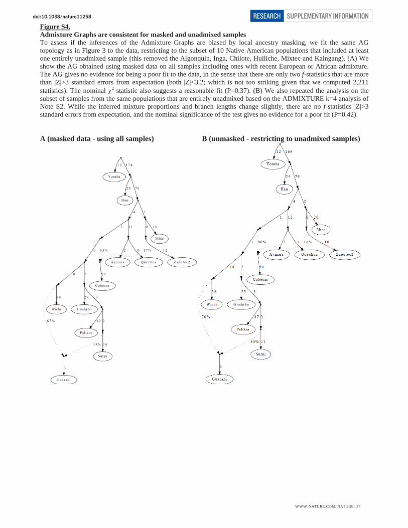
Figure S4.Admixture Graphs are consistent for masked and unadmixed samples To assess if the inferences of the Admixture Graphs are biased by local ancestry masking, we fit the same AG topology as in Figure 3 to the data, restricting to the subset of 10 Native American populations that included at least one entirely unadmixed sample (this removed the Algonquin, Inga, Chilote, Hulliche, Mixtec and Kaingang). (A) We show the AG obtained using masked data on all samples including ones with recent European or African admixture. The AG gives no evidence for being a poor fit to the data, in the sense that there are only two f-statistics that are more than |Z|>3 standard errors from expectation (both |Z|<3.2; which is not too striking given that we computed 2,211 statistics). The nominal 2 statistic also suggests a reasonable fit (P=0.37). (B) We also repeated the analysis on the subset of samples from the same populations that are entirely unadmixed based on the ADMIXTURE k=4 analysis of Note S2. While the inferred mixture proportions and branch lengths change slightly, there are no f-statistics |Z|>3 standard errors from expectation, and the nominal significance of the test gives no evidence for a poor fit (P=0.42).

A (masked data - using all samples) B (unmasked - restricting to unadmixed samples)



Figu

re S

5. H

eter

ozyg

osity

and

dis

tanc

e fr

om th

e B

erin

g St

rait.

A

t the

top

we

show

the

squa

re o

f the

cor

rela

tion

(R2 ) b

etw

een

mea

n po

pula

tion

hete

rozy

gosi

ty a

nd d

ista

nce

from

the

Ber

ing

Stra

it, re

stric

ting

to p

opul

atio

ns w

ith

at le

ast 5

indi

vidu

als

geno

type

d. In

add

ition

to G

reat

Arc

dis

tanc

es, w

e us

ed th

e fo

llow

ing

coas

tline

/inla

nd c

ost c

ombi

natio

ns a

s “e

ffec

tive

dist

ance

s”: 1

:2, 1

:5,

1:10

, 1:2

0, 1

:30,

1:4

0, 1

:50,

1:1

00, 1

:200

, 1:3

00, 1

:400

and

1:5

00. C

orre

latio

ns w

ith P

-val

ues

<0.0

5 ar

e sh

own

in r

ed. A

t the

bot

tom

we

show

sca

tter-

plot

s of

he

tero

zygo

sity

and

eff

ectiv

e di

stan

ce fr

om th

e B

erin

g St

rait

at th

e co

asta

l/inl

and

cost

ratio

max

imiz

ing

the

hete

rozy

gosi

ty-d

istan

ce c

orre

latio

n. T

he x

-axi

s in

the

scat

terp

lots

is in

uni

ts o

f ef

fect

ive

dist

ance

, with

no

spec

ific

mea

ning

for

the

abso

lute

val

ues.

(A)

Show

s re

sults

for

all

popu

latio

ns a

cros

s th

e A

mer

icas

. (B

) Ex

clud

es th

e N

orth

Am

eric

an p

opul

atio

ns w

ith e

vide

nce

of a

nces

try fr

om la

ter s

tream

s of

gen

e flo

w fr

om A

sia.

(C) S

how

s re

sults

whe

n C

hibc

han

popu

latio

ns

from

the

Isth

mo-

Col

ombi

an a

rea

are

also

exc

lude

d (C

hibc

han

spea

kers

show

evi

denc

e of

bac

k-m

igra

tion

from

Sou

th A

mer

ica

into

Cen

tral A

mer

ica)

.

WW

W.N

ATU

RE.C

OM

/NAT

URE

|38

doi:10.1038/n

ature

SUPP

LEM

ENTA

RY IN

FORM

ATIO

NRE

SEAR

CH

Tab

le S

1. S

umm

ary

data

for

52 N

ativ

e A

mer

ican

pop

ulat

ions

Popu

latio

nN

Unadmixed

Langua

gefamily

1Samplinglocatio

nLatitud

eLongitu

deStud

y%Afr2

k=4

%Eu

ro2

k=4

Prop

ortio

nMasked3

Hetero

zygosity

Maxim

um|Z|scoreov

erup

to13

5f 4s

tatistic

stestingforn

onFirstA

merican

ancestry

3Ho

telling

Ttestforn

onFirst

American

ancestry

(Pvalue)

3

Masking

Anc.subtract

Una

dmixed

Masking

Una

dmixed

Aleu

tian

80

EskimoAleu

tUSA

5217

6.6

Willersle

v0.00

000.64

820.92

80.26

04.9

7.7

.9x10

5.

Algonq

uin

50

NorthernAm

erind

Canada

48.4

71.1

This

0.00

000.28

610.48

40.23

72.3

3.1

.0.17

.Arara

11

GePano

Carib

Brazil

453

.5Th

is0.00

000.00

000.03

30.18

03.2

2.6

2.6

0.00

570.16

Arhu

aco

50

Chibchan

Paezan

Colombia

1173

.8Th

is0.05

870.16

720.43

50.20

82.0

3.1

.0.75

.Ay

mara

234

Ande

anBo

livia&Ch

ile16

.5/22

68.2/70

This

0.00

080.02

750.07

50.24

42.9

3.3

2.6

0.18

0.35

Bribri

42

Chibchan

Paezan

CostaRica

9.4

83.1

This

0.02

170.01

070.07

60.22

32.8

2.9

2.0

0.29

0.81

Cabe

car

3124

Chibchan

Paezan

CostaRica

9.5

84Th

is0.00

770.00

880.03

90.22

12.4

2.6

2.7

0.70

0.68

Chane

22

Equatoria

lTucanoan

Argentina

22.3

63.7

This

0.00

000.00

000.01

40.24

72.8

3.0

3.0

0.15

0.27

Chilote

80

Ande

anCh

ile42

.573

.9Th

is0.00

940.37

730.65

70.23

82.6

2.8

.0.28

.Ch

ipew

yan

152

NaDe

neCanada

59.6

107.3

This

0.00

000.18

930.34

00.25

16.0

6.1

5.5

<10

91x10

7

Chon

o4

0An

dean

Chile

4574

This

0.00

410.29

600.54

30.22

73.1

2.4

.0.05

6.

Chorotega

10

CentralA

merind

CostaRica

10.1

85.5

This

0.12

260.12

430.48

70.22

42.4

2.5

.0.86

.Cree

40

NorthernAm

erind

Canada

50.3

102.5

This

0.00

040.37

930.63

90.26

22.4

2.7

.0.21

.Diaguita

50

Ande

anArgentina

28.5

65.8

This

0.02

630.22

570.48

40.24

32.0

2.3

.0.69

.E.Green.Inuit

73

EskimoAleu

tGreenland

67.5

37.9

Willersle

v0.00

000.06

900.17

60.24

716

.416

.315

.0<10

9<1

09

Embe

ra5

5Ch

ibchan

Paezan

Colombia

776

This

0.00

000.00

000.00

40.22

12.6

2.6

2.6

0.85

0.95

Guahibo

66

Equatoria

lTucanoan

Colombia

5.8

69.5

Kidd

0.00

000.00

000.00

30.23

03.2

3.2

3.2

0.30

0.21

Guarani

63

Equatoria

lTucanoan

Paraguay

&Argentina

23/22

.554

/63

.8Th

is0.00

090.08

550.14

80.24

62.9

2.9

3.0

0.06

0.13

Guaymi

55

Chibchan

Paezan

CostaRica

8.5

82Th

is0.00

000.00

000.00

90.21

42.3

2.6

2.6

0.56

0.29

Huetar

10

Chibchan

Paezan

CostaRica

9.7

84.3

This

0.01

870.24

020.46

80.20

92.7

2.5

.0.23

.Hu

lliche

40

Ande

anCh

ile41

73Th

is0.00

490.10

930.24

70.23

42.8

3.0

.0.06

8.

Inga

90

Ande

anCo

lombia

177

This

0.00

440.11

070.25

50.23

02.5

2.1

.0.66

.Jamam

adi

11

Equatoria

lTucanoan

Brazil

8.5

64.5

This

0.00

000.00

000.00

70.20

92.0

2.8

2.8

0.58

0.66

Kaingang

20

GePano

Carib

Brazil

2452

.5Th

is0.03

490.12

050.33

20.22

31.9

2.4

.0.67

.Kaqchikel

131

NorthernAm

erind

Guatem

ala

1591

This

0.01

880.06

570.18

20.25

02.1

2.2

3.3

0.53

0.08

8Karitiana

1313

Equatoria

lTucanoan

Brazil

1063

HGDP

&Kidd

0.00

000.00

000.00

10.22

12.1

2.4

2.4

0.56

0.33

Kogi

44

Chibchan

Paezan

Colombia

1174

This

0.00

000.00

000.00

10.22

01.8

2.2

2.2

0.47

0.33

Maleku

32

Chibchan

Paezan

CostaRica

10.6

84.8

This

0.00

690.01

820.05

80.18

63.5

3.1

2.9

0.18

0.29

Maya1

371

NorthernAm

erind

Mexico

20.3/19.6

87.8/90

.4HG

DP&MGD

P0.01

230.09

040.21

20.25

02.1

2.4

3.1

0.60

0.34

Maya2

120

NorthernAm

erind

Mexico

19.6

90.4

MGD

P0.01

400.06

500.16

90.24

83.1

2.9

.7x10

4.

Mixe

179

NorthernAm

erind

Mexico

1796

This

0.00

130.00

390.02

80.24

22.9

2.8

2.0

0.13

0.54

Mixtec

50

CentralA

merind

Mexico

1797

This

0.00

880.03

220.09

60.24

73.2

2.7

.0.11

.Ojibwa

50

NorthernAm

erind

Canada

46.5

81Th

is0.00

000.27

450.49

00.25

94.0

4.2

.0.01

5.

Palikur

32

Equatoria

lTucanoan

Guiana

451

.8Th

is0.00

000.01

420.03

30.21

83.1

2.4

2.1

0.14

0.79

Parakana

11

Equatoria

lTucanoan

Brazil

4.8

50Th

is0.00

000.00

000.00

30.23

52.7

2.8

2.8

0.60

0.81

Piapoco

76

Equatoria

lTucanoan

Colombia

368

HGDP

0.00

740.01

210.04

30.23

52.8

2.6

2.9

0.12

0.33

Pima

3314

CentralA

merind

Mexico

29.3

108.8

HGDP

&Kidd

0.00

140.03

210.08

10.23

73.7

3.5

3.7

0.02

30.33

Purepe

cha

10

Chibchan

Paezan

Mexico

1910

1.5

This

0.02

230.14

890.33

70.25

53.4

3.0

.0.04

2.

Que

chua

401

Ande

anBo

livia&Pe

ru14

.5/14

69/74

This

0.00

430.07

600.17

30.24

42.6

2.4

2.5

0.37

0.54

Surui

2424

Equatoria

lTucanoan

Brazil

1162

HGDP

0.00

000.00

000.00

00.20

61.8

2.1

2.1

0.92

0.79

Tepe

huano

252

CentralA

merind

Mexico

23.2

104.5

MGD

P0.00

240.03

710.09

50.24

62.2

2.7

2.2

0.58

0.43

Terib

e3

2Ch

ibchan

Paezan

CostaRica

983

.2Th

is0.00

290.00

000.01

20.21

72.5

2.4

2.3

0.52

0.84

Ticuna

65

Equatoria

lTucanoan

Colombia

3.81

70.01

This

0.00

960.00

360.04

70.22

52.1

1.9

2.3

0.62

0.70

Toba

42

GePano

Carib

Argentina

26.5

59.3

This

0.00

000.01

140.04

00.24

32.7

2.6

3.2

0.36

0.02

5Wauna

na3

3Ch

ibchan

Paezan

Colombia

577

This

0.00

000.00

000.01

40.23

32.1

2.1

2.1

0.65

0.56

Wayuu

113

Equatoria

lTucanoan

Colombia

1173

This

0.03

510.06

670.21

10.23

43.3

3.6

4.4

0.02

80.09

9W.G

reen

.Inu

it8

0EskimoAleu

tGreenland

65.3

52Willersle

v0.00

000.26

960.51

30.24

916

.516

.6.

<10

9.

Wichi

54

GePano

Carib

Argentina

22.5

63.8

This

0.00

090.02

360.05

30.22

02.4

2.8

3.0

0.35

0.04

1Yaghan

41

Ande

anCh

ile55

68Th

is0.00

430.15

610.34

90.23

42.6

2.2

2.3

0.24

0.36

Yaqu

i1

0Ce

ntralA

merind

Mexico

2811

0.3

This

0.01

180.16

510.42

40.22

43.1

2.6

.0.12

.Zapo

tec1

222

CentralA

merind

Mexico

16.5/16

97.2/97

This

0.00

520.06

570.15

60.24

82.0

2.1

2.0

0.94

0.65

Zapo

tec2

213

CentralA

merind

Mexico

17.4

96.7

MGD

P0.00

030.01

210.04

40.24

62.0

2.5

2.5

0.60

0.26

1For“language

family”,weuseGreenb

erg’sc

lassificatio

nof

the“sup

erfamily”Am

erindinto

7subfam

ilies.

2Estim

ateof

Europe

anandAfrican

ancestry

from

ADMIXTU

REk=4(NoteS2).

3Theprop

ortio

nof

thegeno

memaskedisbasedon

HAPM

IXlocalancestryinference(NoteS4).

3The13

5=45

x3po

ssiblef 4(Una

dmixed,Test;Outgrou

p1,O

utroup

2;)statisticsa

rebasedon

45=10

x9/2

possiblepairs

ofou

tgroup

s(9Sibe

rianwith

10samples

andHa

n),and

3Un

admixed

popu

latio

ns(Karitiana,Gu

aymi,andapo

olof

158samples).Wehighlight

inyellowcasesw

here

the

maxim

umstatisticis|Z

max|>4.5correspo

ndingto

P<0.00

5aftercorrectingform

ultip

lehypo

thesistesting,or

whe

retheHo

telling

TtestP<

0.00

5.[

WW

W.N

ATU

RE.C

OM

/NAT

URE

|39

doi:10.1038/n

ature

SUPP

LEM

ENTA

RY IN

FORM

ATIO

NRE

SEAR

CH

Tab

le S

2. S

umm

ary

data

for

17 S

iber

ian

popu

latio

ns

Popu

latio

nN

Lang

uage

family

1Sampling

locatio

nLatitud

eLongi

tude

Stud

yProp

ortio

nMasked2

Hetero

zygosity

Altaian

12Altaic

Russia

56.3

82.8

Willersle

v0.66

20.27

8Bu

ryat

17Altaic

Russia

52.6

104.3

Willersle

v0.38

50.27

8Ch

ukchi

30Ch

ukchiK

amchatkan

Russia

67.8(69)

178.4(17

0)Willersle

v&Di

Rien

zo0.01

00.26

8Do

lgan

4Altaic

Russia

69.8

88.1

Willersle

v0.38

90.27

1Even

ki15

Altaic

Russia

64.1

95.4

Willersle

v0.21

10.27

5Ke

t2

Isolate

Russia

63.8

87.4

Willersle

v0.55

20.27

1Kh

anty

35Uralic

Yukaghir

Russia

6376

.5Kidd

0.68

10.27

1Ko

ryak

10Ch

ukchiK

amchatkan

Russia

64.1

167.9

Willersle

v0.00

80.26

1Mon

golian

8Altaic

Mon

golia

4810

7Willersle

v0.59

40.28

0Naukan

16EskimoAleu

tRu

ssia

6518

8Di

Rien

zo0.00

30.26

1Nganasan1

8Uralic

Yukaghir

Russia

73.3

88Willersle

v0.07

90.26

1Nganasan2

14Uralic

Yukaghir

Russia

7094

DiRien

zo0.05

50.26

0Selkup

9Uralic

Yukaghir

Russia

66.4

84.9

Willersle

v0.59

10.27

1Tund

raNen

tsi

3Uralic

Yukaghir

Russia

66.1

76.5

Thisstud

y0.46

50.27

4Tuvinians

15Altaic

Russia

5294

.4Willersle

v0.44

90.28

0Yakut

34Altaic

Russia

6313

0HG

DPandKidd

0.25

10.27

5Yukaghir

13Uralic

Yukaghir

Russia

6815

0Di

Rien

zo0.10

00.27

31Language

classificationfollowsR

uhlen1991.

2Theprop

ortio

nof

thegeno

memasked(onlydo

neinthemaskeddataset)isbasedon

removingsegm

entswhe

rethepo

steriore

stim

ateof

thenu

mbe

rofn

onNativechromosom

esis>0.01.Themasking

oftheSibe

riansamples

ispe

rformed

simultane

ously

with

themasking

oftheNativeAm

erican

samples.

WW

W.N

ATU

RE.C

OM

/NAT

URE

|40

doi:10.1038/n

ature

SUPP

LEM

ENTA

RY IN

FORM

ATIO

NRE

SEAR

CH

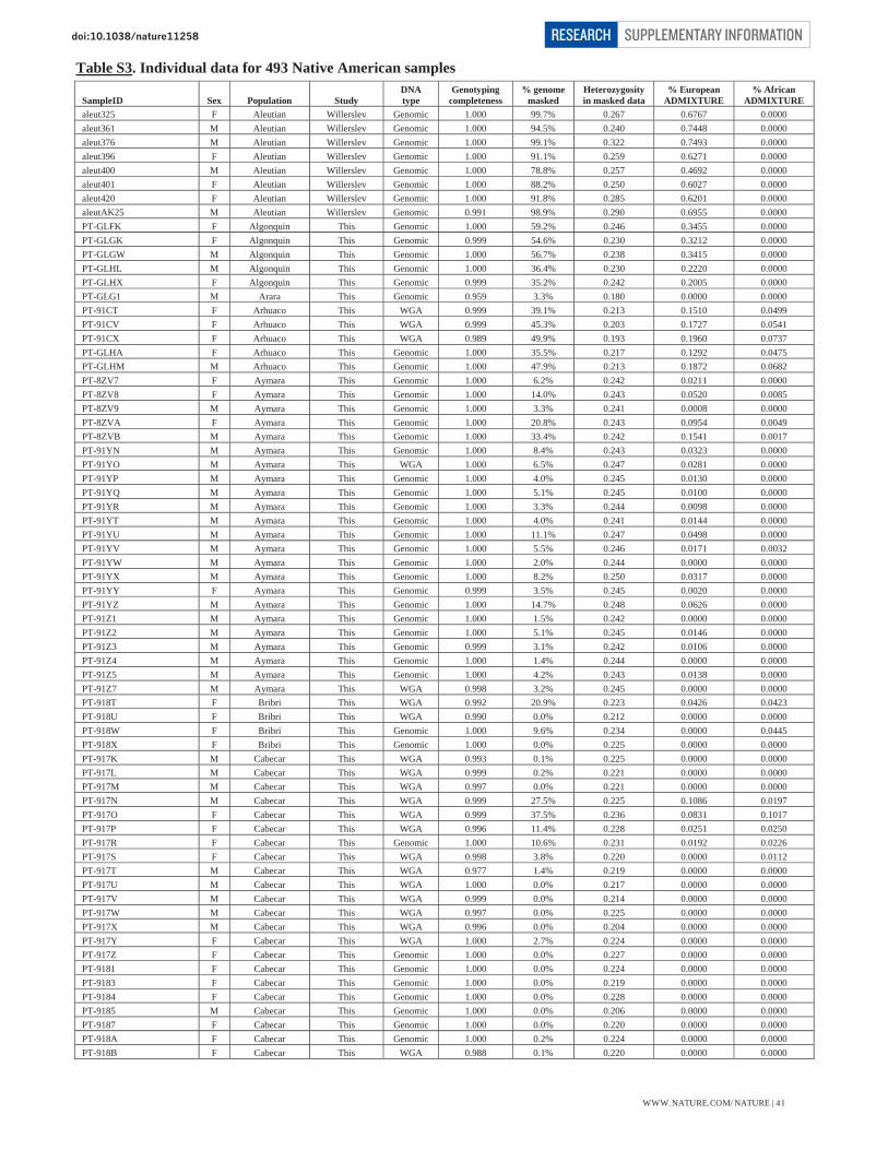
Table S3. Individual data for 493 Native American samples

SampleID Sex Population Study DNAtype

Genotyping completeness

% genome masked

Heterozygosity in masked data

% European ADMIXTURE

% African ADMIXTURE

aleut325 F Aleutian Willerslev Genomic 1.000 99.7% 0.267 0.6767 0.0000 aleut361 M Aleutian Willerslev Genomic 1.000 94.5% 0.240 0.7448 0.0000 aleut376 M Aleutian Willerslev Genomic 1.000 99.1% 0.322 0.7493 0.0000 aleut396 F Aleutian Willerslev Genomic 1.000 91.1% 0.259 0.6271 0.0000 aleut400 M Aleutian Willerslev Genomic 1.000 78.8% 0.257 0.4692 0.0000 aleut401 F Aleutian Willerslev Genomic 1.000 88.2% 0.250 0.6027 0.0000 aleut420 F Aleutian Willerslev Genomic 1.000 91.8% 0.285 0.6201 0.0000 aleutAK25 M Aleutian Willerslev Genomic 0.991 98.9% 0.290 0.6955 0.0000 PT-GLFK F Algonquin This Genomic 1.000 59.2% 0.246 0.3455 0.0000 PT-GLGK F Algonquin This Genomic 0.999 54.6% 0.230 0.3212 0.0000 PT-GLGW M Algonquin This Genomic 1.000 56.7% 0.238 0.3415 0.0000 PT-GLHL M Algonquin This Genomic 1.000 36.4% 0.230 0.2220 0.0000 PT-GLHX F Algonquin This Genomic 0.999 35.2% 0.242 0.2005 0.0000 PT-GLG1 M Arara This Genomic 0.959 3.3% 0.180 0.0000 0.0000 PT-91CT F Arhuaco This WGA 0.999 39.1% 0.213 0.1510 0.0499 PT-91CV F Arhuaco This WGA 0.999 45.3% 0.203 0.1727 0.0541 PT-91CX F Arhuaco This WGA 0.989 49.9% 0.193 0.1960 0.0737 PT-GLHA F Arhuaco This Genomic 1.000 35.5% 0.217 0.1292 0.0475 PT-GLHM M Arhuaco This Genomic 1.000 47.9% 0.213 0.1872 0.0682 PT-8ZV7 F Aymara This Genomic 1.000 6.2% 0.242 0.0211 0.0000 PT-8ZV8 F Aymara This Genomic 1.000 14.0% 0.243 0.0520 0.0085 PT-8ZV9 M Aymara This Genomic 1.000 3.3% 0.241 0.0008 0.0000 PT-8ZVA F Aymara This Genomic 1.000 20.8% 0.243 0.0954 0.0049 PT-8ZVB M Aymara This Genomic 1.000 33.4% 0.242 0.1541 0.0017 PT-91YN M Aymara This Genomic 1.000 8.4% 0.243 0.0323 0.0000 PT-91YO M Aymara This WGA 1.000 6.5% 0.247 0.0281 0.0000 PT-91YP M Aymara This Genomic 1.000 4.0% 0.245 0.0130 0.0000 PT-91YQ M Aymara This Genomic 1.000 5.1% 0.245 0.0100 0.0000 PT-91YR M Aymara This Genomic 1.000 3.3% 0.244 0.0098 0.0000 PT-91YT M Aymara This Genomic 1.000 4.0% 0.241 0.0144 0.0000 PT-91YU M Aymara This Genomic 1.000 11.1% 0.247 0.0498 0.0000 PT-91YV M Aymara This Genomic 1.000 5.5% 0.246 0.0171 0.0032 PT-91YW M Aymara This Genomic 1.000 2.0% 0.244 0.0000 0.0000 PT-91YX M Aymara This Genomic 1.000 8.2% 0.250 0.0317 0.0000 PT-91YY F Aymara This Genomic 0.999 3.5% 0.245 0.0020 0.0000 PT-91YZ M Aymara This Genomic 1.000 14.7% 0.248 0.0626 0.0000 PT-91Z1 M Aymara This Genomic 1.000 1.5% 0.242 0.0000 0.0000 PT-91Z2 M Aymara This Genomic 1.000 5.1% 0.245 0.0146 0.0000 PT-91Z3 M Aymara This Genomic 0.999 3.1% 0.242 0.0106 0.0000 PT-91Z4 M Aymara This Genomic 1.000 1.4% 0.244 0.0000 0.0000 PT-91Z5 M Aymara This Genomic 1.000 4.2% 0.243 0.0138 0.0000 PT-91Z7 M Aymara This WGA 0.998 3.2% 0.245 0.0000 0.0000 PT-918T F Bribri This WGA 0.992 20.9% 0.223 0.0426 0.0423 PT-918U F Bribri This WGA 0.990 0.0% 0.212 0.0000 0.0000 PT-918W F Bribri This Genomic 1.000 9.6% 0.234 0.0000 0.0445 PT-918X F Bribri This Genomic 1.000 0.0% 0.225 0.0000 0.0000 PT-917K M Cabecar This WGA 0.993 0.1% 0.225 0.0000 0.0000 PT-917L M Cabecar This WGA 0.999 0.2% 0.221 0.0000 0.0000 PT-917M M Cabecar This WGA 0.997 0.0% 0.221 0.0000 0.0000 PT-917N M Cabecar This WGA 0.999 27.5% 0.225 0.1086 0.0197 PT-917O F Cabecar This WGA 0.999 37.5% 0.236 0.0831 0.1017 PT-917P F Cabecar This WGA 0.996 11.4% 0.228 0.0251 0.0250 PT-917R F Cabecar This Genomic 1.000 10.6% 0.231 0.0192 0.0226 PT-917S F Cabecar This WGA 0.998 3.8% 0.220 0.0000 0.0112 PT-917T M Cabecar This WGA 0.977 1.4% 0.219 0.0000 0.0000 PT-917U M Cabecar This WGA 1.000 0.0% 0.217 0.0000 0.0000 PT-917V M Cabecar This WGA 0.999 0.0% 0.214 0.0000 0.0000 PT-917W M Cabecar This WGA 0.997 0.0% 0.225 0.0000 0.0000 PT-917X M Cabecar This WGA 0.996 0.0% 0.204 0.0000 0.0000 PT-917Y F Cabecar This WGA 1.000 2.7% 0.224 0.0000 0.0000 PT-917Z F Cabecar This Genomic 1.000 0.0% 0.227 0.0000 0.0000 PT-9181 F Cabecar This Genomic 1.000 0.0% 0.224 0.0000 0.0000 PT-9183 F Cabecar This Genomic 1.000 0.0% 0.219 0.0000 0.0000 PT-9184 F Cabecar This Genomic 1.000 0.0% 0.228 0.0000 0.0000 PT-9185 M Cabecar This Genomic 1.000 0.0% 0.206 0.0000 0.0000 PT-9187 F Cabecar This Genomic 1.000 0.0% 0.220 0.0000 0.0000 PT-918A F Cabecar This Genomic 1.000 0.2% 0.224 0.0000 0.0000 PT-918B F Cabecar This WGA 0.988 0.1% 0.220 0.0000 0.0000



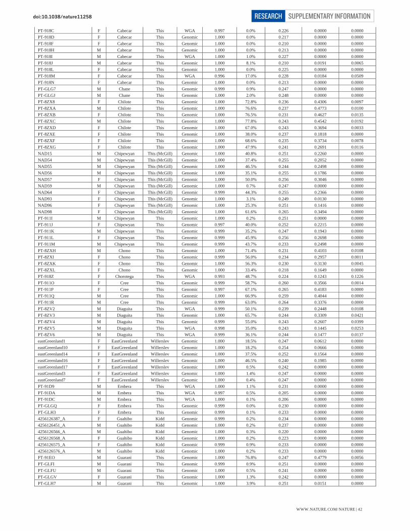
PT-918C F Cabecar This WGA 0.997 0.0% 0.226 0.0000 0.0000 PT-918D F Cabecar This Genomic 1.000 0.0% 0.217 0.0000 0.0000 PT-918F F Cabecar This Genomic 1.000 0.0% 0.210 0.0000 0.0000 PT-918H M Cabecar This Genomic 1.000 0.0% 0.213 0.0000 0.0000 PT-918I M Cabecar This WGA 1.000 1.0% 0.227 0.0000 0.0000 PT-918J M Cabecar This Genomic 1.000 8.1% 0.210 0.0191 0.0065 PT-918L F Cabecar This Genomic 1.000 0.0% 0.225 0.0000 0.0000 PT-918M F Cabecar This WGA 0.996 17.0% 0.228 0.0184 0.0509 PT-918N F Cabecar This Genomic 1.000 0.0% 0.213 0.0000 0.0000 PT-GLG7 M Chane This Genomic 0.999 0.9% 0.247 0.0000 0.0000 PT-GLGJ M Chane This Genomic 1.000 2.0% 0.248 0.0000 0.0000 PT-8ZX8 F Chilote This Genomic 1.000 72.8% 0.236 0.4306 0.0097 PT-8ZXA M Chilote This Genomic 1.000 76.6% 0.237 0.4773 0.0100 PT-8ZXB F Chilote This Genomic 1.000 76.5% 0.231 0.4627 0.0135 PT-8ZXC M Chilote This Genomic 1.000 77.8% 0.243 0.4542 0.0192 PT-8ZXD F Chilote This Genomic 1.000 67.0% 0.243 0.3694 0.0033 PT-8ZXE F Chilote This Genomic 1.000 38.0% 0.237 0.1818 0.0000 PT-8ZXF F Chilote This Genomic 1.000 68.6% 0.235 0.3734 0.0078 PT-8ZXG F Chilote This Genomic 1.000 47.9% 0.241 0.2691 0.0116 NAD15 M Chipewyan This (McGill) Genomic 1.000 40.8% 0.251 0.2260 0.0000 NAD54 M Chipewyan This (McGill) Genomic 1.000 37.4% 0.255 0.2052 0.0000 NAD55 M Chipewyan This (McGill) Genomic 1.000 46.5% 0.244 0.2498 0.0000 NAD56 M Chipewyan This (McGill) Genomic 1.000 35.1% 0.255 0.1786 0.0000 NAD57 F Chipewyan This (McGill) Genomic 1.000 50.0% 0.256 0.3046 0.0000 NAD59 M Chipewyan This (McGill) Genomic 1.000 0.7% 0.247 0.0000 0.0000 NAD64 F Chipewyan This (McGill) Genomic 0.999 44.3% 0.255 0.2366 0.0000 NAD93 F Chipewyan This (McGill) Genomic 1.000 3.1% 0.249 0.0130 0.0000 NAD96 F Chipewyan This (McGill) Genomic 1.000 25.3% 0.251 0.1416 0.0000 NAD98 F Chipewyan This (McGill) Genomic 1.000 61.6% 0.265 0.3494 0.0000 PT-911I M Chipewyan This Genomic 1.000 0.2% 0.251 0.0000 0.0000 PT-911J F Chipewyan This Genomic 0.997 40.0% 0.252 0.2215 0.0000 PT-911K M Chipewyan This Genomic 0.999 35.2% 0.247 0.1943 0.0000 PT-911L F Chipewyan This Genomic 0.999 45.9% 0.256 0.2698 0.0000 PT-911M M Chipewyan This Genomic 0.999 43.7% 0.233 0.2498 0.0000 PT-8ZXH M Chono This Genomic 1.000 71.4% 0.231 0.4103 0.0108 PT-8ZXI F Chono This Genomic 0.999 56.0% 0.234 0.2957 0.0011 PT-8ZXK F Chono This Genomic 1.000 56.3% 0.230 0.3130 0.0045 PT-8ZXL F Chono This Genomic 1.000 33.4% 0.218 0.1649 0.0000 PT-918Z F Chorotega This WGA 0.993 48.7% 0.224 0.1243 0.1226 PT-911O F Cree This Genomic 0.999 58.7% 0.260 0.3566 0.0014 PT-911P F Cree This Genomic 0.997 67.1% 0.265 0.4183 0.0000 PT-911Q M Cree This Genomic 1.000 66.9% 0.259 0.4044 0.0000 PT-911R M Cree This Genomic 0.999 63.0% 0.264 0.3376 0.0000 PT-8ZV2 M Diaguita This WGA 0.999 50.1% 0.239 0.2448 0.0108 PT-8ZV3 M Diaguita This Genomic 1.000 65.7% 0.244 0.3309 0.0421 PT-8ZV4 M Diaguita This Genomic 0.999 55.0% 0.243 0.2607 0.0399 PT-8ZV5 M Diaguita This WGA 0.998 35.0% 0.243 0.1445 0.0253 PT-8ZV6 M Diaguita This WGA 0.999 36.1% 0.244 0.1477 0.0137 eastGreenland1 F EastGreenland Willerslev Genomic 1.000 18.5% 0.247 0.0612 0.0000 eastGreenland10 F EastGreenland Willerslev Genomic 1.000 18.2% 0.254 0.0666 0.0000 eastGreenland14 F EastGreenland Willerslev Genomic 1.000 37.5% 0.252 0.1564 0.0000 eastGreenland16 F EastGreenland Willerslev Genomic 1.000 46.5% 0.240 0.1985 0.0000 eastGreenland17 F EastGreenland Willerslev Genomic 1.000 0.5% 0.242 0.0000 0.0000 eastGreenland3 F EastGreenland Willerslev Genomic 1.000 1.4% 0.247 0.0000 0.0000 eastGreenland7 F EastGreenland Willerslev Genomic 1.000 0.4% 0.247 0.0000 0.0000 PT-91D9 M Embera This WGA 1.000 1.1% 0.231 0.0000 0.0000 PT-91DA M Embera This WGA 0.997 0.5% 0.205 0.0000 0.0000 PT-91DC M Embera This WGA 1.000 0.1% 0.206 0.0000 0.0000 PT-GLGQ F Embera This Genomic 0.999 0.0% 0.230 0.0000 0.0000 PT-GLH3 F Embera This Genomic 0.999 0.1% 0.233 0.0000 0.0000 4256126387_A F Guahibo Kidd Genomic 0.999 0.2% 0.234 0.0000 0.0000 4256126451_A M Guahibo Kidd Genomic 1.000 0.2% 0.237 0.0000 0.0000 4256126566_A M Guahibo Kidd Genomic 1.000 0.3% 0.220 0.0000 0.0000 4256126568_A F Guahibo Kidd Genomic 1.000 0.2% 0.223 0.0000 0.0000 4256126575_A F Guahibo Kidd Genomic 0.999 0.9% 0.233 0.0000 0.0000 4256126576_A M Guahibo Kidd Genomic 1.000 0.2% 0.233 0.0000 0.0000 PT-91EO M Guarani This Genomic 1.000 76.8% 0.247 0.4779 0.0056 PT-GLFI M Guarani This Genomic 0.999 0.9% 0.251 0.0000 0.0000 PT-GLFU M Guarani This Genomic 1.000 0.5% 0.241 0.0000 0.0000 PT-GLGV F Guarani This Genomic 1.000 1.3% 0.242 0.0000 0.0000 PT-GLH7 M Guarani This Genomic 1.000 3.9% 0.251 0.0151 0.0000



PT-GLHJ M Guarani This Genomic 0.990 5.1% 0.247 0.0199 0.0000 PT-917E M Guaymi This WGA 0.999 1.1% 0.222 0.0000 0.0000 PT-917F M Guaymi This WGA 0.999 0.0% 0.206 0.0000 0.0000 PT-917G M Guaymi This WGA 0.999 0.2% 0.218 0.0000 0.0000 PT-917H M Guaymi This WGA 0.993 2.5% 0.209 0.0000 0.0000 PT-917I F Guaymi This Genomic 1.000 0.5% 0.214 0.0000 0.0000 PT-9193 F Huetar This WGA 0.993 46.8% 0.209 0.2402 0.0187 PT-8ZVD F Hulliche This Genomic 1.000 4.5% 0.237 0.0179 0.0000 PT-8ZVE F Hulliche This Genomic 1.000 30.7% 0.235 0.1345 0.0039 PT-8ZVF F Hulliche This Genomic 0.983 32.4% 0.225 0.1213 0.0156 PT-8ZVG F Hulliche This Genomic 1.000 31.2% 0.239 0.1637 0.0000 PT-919J M Inga This WGA 1.000 13.9% 0.232 0.0536 0.0078 PT-919P M Inga This Genomic 1.000 12.8% 0.224 0.0576 0.0000 PT-91CH F Inga This Genomic 1.000 30.7% 0.234 0.1398 0.0054 PT-91CL F Inga This WGA 0.983 31.3% 0.219 0.1374 0.0000 PT-91CM M Inga This Genomic 1.000 10.2% 0.236 0.0436 0.0019 PT-91CN M Inga This Genomic 1.000 8.8% 0.235 0.0361 0.0000 PT-91CO F Inga This Genomic 1.000 11.5% 0.225 0.0537 0.0000 PT-91CP F Inga This Genomic 1.000 63.9% 0.250 0.2793 0.0245 PT-91CS F Inga This WGA 0.959 47.9% 0.218 0.1955 0.0000 PT-9GRL M Jamamadi This Genomic 0.998 0.7% 0.209 0.0000 0.0000 PT-91ET F Kaingang This Genomic 0.998 31.1% 0.216 0.0988 0.0491 PT-91EU F Kaingang This Genomic 0.995 35.4% 0.231 0.1422 0.0207 PT-9143 M Kaqchikel This Genomic 1.000 2.2% 0.246 0.0003 0.0000 PT-9147 F Kaqchikel This Genomic 1.000 58.8% 0.248 0.1292 0.1735 PT-9148 F Kaqchikel This Genomic 1.000 24.0% 0.250 0.1070 0.0020 PT-916Z F Kaqchikel This Genomic 1.000 7.7% 0.253 0.0289 0.0000 PT-9171 F Kaqchikel This WGA 0.997 26.2% 0.249 0.1142 0.0090 PT-9172 F Kaqchikel This WGA 0.996 2.3% 0.248 0.0000 0.0000 PT-9173 M Kaqchikel This WGA 0.996 12.4% 0.248 0.0510 0.0007 PT-9174 M Kaqchikel This Genomic 0.997 54.9% 0.251 0.2420 0.0475 PT-9176 F Kaqchikel This Genomic 1.000 4.4% 0.254 0.0137 0.0000 PT-9179 M Kaqchikel This Genomic 0.999 15.8% 0.253 0.0690 0.0016 PT-917A M Kaqchikel This Genomic 1.000 5.2% 0.251 0.0136 0.0000 PT-917B M Kaqchikel This Genomic 1.000 16.2% 0.252 0.0621 0.0098 PT-917C F Kaqchikel This Genomic 0.998 6.8% 0.245 0.0240 0.0000 HGDP00995 F Karitiana HGDP Genomic 1.000 0.0% 0.229 0.0000 0.0000 HGDP00998 M Karitiana HGDP Genomic 1.000 0.1% 0.219 0.0000 0.0000 HGDP00999 F Karitiana HGDP Genomic 1.000 0.1% 0.225 0.0000 0.0000 HGDP01001 F Karitiana HGDP Genomic 1.000 0.1% 0.231 0.0000 0.0000 HGDP01003 F Karitiana HGDP Genomic 1.000 0.2% 0.224 0.0000 0.0000 HGDP01006 F Karitiana HGDP Genomic 1.000 0.0% 0.221 0.0000 0.0000 HGDP01010 F Karitiana HGDP Genomic 1.000 0.0% 0.236 0.0000 0.0000 HGDP01012 M Karitiana HGDP Genomic 1.000 0.1% 0.214 0.0000 0.0000 HGDP01013 M Karitiana HGDP Genomic 1.000 0.0% 0.225 0.0000 0.0000 HGDP01014 F Karitiana HGDP Genomic 1.000 0.0% 0.215 0.0000 0.0000 HGDP01015 M Karitiana HGDP Genomic 1.000 0.1% 0.223 0.0000 0.0000 HGDP01018 F Karitiana HGDP Genomic 1.000 0.0% 0.217 0.0000 0.0000 HGDP01019 M Karitiana HGDP Genomic 1.000 0.0% 0.201 0.0000 0.0000 PT-91D6 M Kogi This WGA 0.996 0.0% 0.213 0.0000 0.0000 PT-GLFW M Kogi This Genomic 0.996 0.0% 0.218 0.0000 0.0000 PT-GLGL M Kogi This Genomic 0.997 0.5% 0.224 0.0000 0.0000 PT-GLGX M Kogi This Genomic 0.998 0.0% 0.224 0.0000 0.0000 PT-9198 F Maleku This WGA 0.998 0.2% 0.176 0.0000 0.0000 PT-9199 M Maleku This WGA 1.000 0.2% 0.190 0.0000 0.0000 PT-919B F Maleku This Genomic 1.000 17.0% 0.194 0.0547 0.0206 HGDP00855 F Maya1 HGDP Genomic 1.000 4.2% 0.248 0.0153 0.0000 HGDP00856 M Maya1 HGDP Genomic 1.000 11.8% 0.254 0.0549 0.0000 HGDP00857 F Maya1 HGDP Genomic 1.000 5.4% 0.243 0.0185 0.0000 HGDP00858 F Maya1 HGDP Genomic 0.993 12.3% 0.250 0.0581 0.0000 HGDP00859 F Maya1 HGDP Genomic 1.000 16.3% 0.252 0.0447 0.0248 HGDP00860 F Maya1 HGDP Genomic 1.000 58.5% 0.255 0.2840 0.0410 HGDP00861 F Maya1 HGDP Genomic 1.000 38.5% 0.248 0.1440 0.0347 HGDP00862 F Maya1 HGDP Genomic 1.000 21.2% 0.252 0.0986 0.0075 HGDP00863 F Maya1 HGDP Genomic 1.000 19.5% 0.252 0.0391 0.0457 HGDP00864 F Maya1 HGDP Genomic 1.000 11.2% 0.255 0.0460 0.0000 HGDP00868 F Maya1 HGDP Genomic 1.000 30.1% 0.255 0.1224 0.0387 HGDP00869 F Maya1 HGDP Genomic 1.000 38.2% 0.235 0.1778 0.0186 HGDP00870 F Maya1 HGDP Genomic 1.000 14.4% 0.250 0.0658 0.0000 HGDP00871 F Maya1 HGDP Genomic 0.999 53.5% 0.250 0.2628 0.0229 HGDP00872 F Maya1 HGDP Genomic 1.000 14.9% 0.247 0.0518 0.0132



HGDP00876 F Maya1 HGDP Genomic 1.000 52.2% 0.253 0.2652 0.0186 HGDP00877 M Maya1 HGDP Genomic 0.999 26.6% 0.252 0.1096 0.0120 Maya_4003_041703 M Maya1 MGDP Genomic 1.000 17.6% 0.248 0.0853 0.0056 Maya_4003_042703 F Maya1 MGDP Genomic 1.000 24.3% 0.253 0.1103 0.0138 Maya_4009_041709 M Maya1 MGDP Genomic 1.000 39.8% 0.249 0.1742 0.0173 Maya_4012_041712 M Maya1 MGDP Genomic 0.999 31.6% 0.246 0.1273 0.0251 Maya_4012_042712 F Maya1 MGDP Genomic 1.000 16.3% 0.251 0.0687 0.0000 Maya_4014_041714 M Maya1 MGDP Genomic 1.000 36.2% 0.249 0.1513 0.0240 Maya_4014_042714 F Maya1 MGDP Genomic 0.999 7.3% 0.248 0.0273 0.0000 Maya_4016_041716 M Maya1 MGDP Genomic 0.995 10.1% 0.250 0.0420 0.0000 Maya_4016_042716 F Maya1 MGDP Genomic 0.999 14.5% 0.251 0.0573 0.0067 Maya_4017_041717 M Maya1 MGDP Genomic 0.998 9.9% 0.251 0.0462 0.0048 Maya_4017_042717 F Maya1 MGDP Genomic 0.991 6.4% 0.249 0.0250 0.0000 Maya_4018_041718 M Maya1 MGDP Genomic 0.995 22.6% 0.252 0.1029 0.0060 Maya_4018_042718 F Maya1 MGDP Genomic 0.999 12.5% 0.250 0.0576 0.0000 Maya_4026_042726 F Maya1 MGDP Genomic 1.000 8.9% 0.254 0.0343 0.0000 Maya_4031_041731 M Maya1 MGDP Genomic 0.999 23.4% 0.254 0.0909 0.0276 Maya_4032_041732 M Maya1 MGDP Genomic 0.999 1.9% 0.249 0.0000 0.0000 Maya_4032_042732 F Maya1 MGDP Genomic 1.000 22.8% 0.248 0.1094 0.0000 Maya_4034_042734 F Maya1 MGDP Genomic 1.000 15.5% 0.248 0.0413 0.0258 Maya_4037_041737 M Maya1 MGDP Genomic 1.000 9.1% 0.253 0.0444 0.0000 Maya_4037_042737 F Maya1 MGDP Genomic 1.000 23.8% 0.252 0.0897 0.0205 Maya_4000_041700 M Maya2 MGDP Genomic 1.000 11.0% 0.244 0.0411 0.0107 Maya_4000_042700 F Maya2 MGDP Genomic 0.979 24.8% 0.238 0.0778 0.0258 Maya_4001_042701 F Maya2 MGDP Genomic 1.000 14.9% 0.247 0.0500 0.0168 Maya_4005_041705 M Maya2 MGDP Genomic 0.999 24.4% 0.247 0.1011 0.0122 Maya_4005_042705 F Maya2 MGDP Genomic 1.000 7.7% 0.240 0.0379 0.0045 Maya_4009_042709 F Maya2 MGDP Genomic 1.000 15.7% 0.250 0.0687 0.0118 Maya_4010_042710 F Maya2 MGDP Genomic 1.000 18.1% 0.250 0.0709 0.0111 Maya_4010_c_041710_c M Maya2 MGDP Genomic 1.000 16.2% 0.249 0.0536 0.0155 Maya_4011_042711 F Maya2 MGDP Genomic 0.996 12.3% 0.254 0.0456 0.0110 Maya_4025_041725 M Maya2 MGDP Genomic 0.995 23.7% 0.251 0.1060 0.0119 Maya_4025_042725 F Maya2 MGDP Genomic 0.999 16.7% 0.249 0.0505 0.0303 Maya_4026_041726 M Maya2 MGDP Genomic 1.000 17.9% 0.252 0.0763 0.0061 PT-912T F Mixe This Genomic 1.000 1.7% 0.245 0.0000 0.0000 PT-912U F Mixe This Genomic 1.000 3.0% 0.237 0.0000 0.0000 PT-912V F Mixe This Genomic 1.000 2.7% 0.245 0.0006 0.0000 PT-912W M Mixe This Genomic 1.000 0.3% 0.244 0.0000 0.0000 PT-912X F Mixe This Genomic 1.000 3.7% 0.249 0.0033 0.0000 PT-912Y F Mixe This Genomic 1.000 3.6% 0.241 0.0126 0.0000 PT-912Z M Mixe This Genomic 1.000 0.7% 0.242 0.0000 0.0000 PT-9131 F Mixe This Genomic 1.000 9.6% 0.238 0.0159 0.0208 PT-9132 F Mixe This Genomic 1.000 3.9% 0.241 0.0003 0.0000 PT-9133 F Mixe This Genomic 1.000 1.6% 0.246 0.0000 0.0000 PT-9134 F Mixe This Genomic 1.000 2.0% 0.241 0.0000 0.0000 PT-9135 F Mixe This Genomic 1.000 1.5% 0.247 0.0000 0.0009 PT-9136 M Mixe This Genomic 1.000 0.5% 0.233 0.0000 0.0000 PT-9137 M Mixe This Genomic 1.000 2.6% 0.238 0.0000 0.0000 PT-9139 F Mixe This Genomic 1.000 3.6% 0.244 0.0108 0.0000 PT-913B F Mixe This Genomic 1.000 2.0% 0.236 0.0000 0.0000 PT-913C M Mixe This Genomic 1.000 5.3% 0.243 0.0226 0.0000 PT-912N F Mixtec This Genomic 1.000 7.6% 0.238 0.0175 0.0161 PT-912O F Mixtec This Genomic 1.000 8.1% 0.247 0.0195 0.0140 PT-912P M Mixtec This Genomic 1.000 6.8% 0.250 0.0250 0.0029 PT-912Q F Mixtec This Genomic 1.000 19.1% 0.244 0.0885 0.0000 PT-912R M Mixtec This Genomic 1.000 6.2% 0.253 0.0103 0.0108 PT-911S F Ojibwa This Genomic 1.000 60.7% 0.259 0.3626 0.0000 PT-911T F Ojibwa This Genomic 1.000 54.0% 0.256 0.3066 0.0000 PT-911U F Ojibwa This WGA 0.998 56.8% 0.258 0.3201 0.0000 PT-911V F Ojibwa This WGA 0.998 32.8% 0.259 0.1787 0.0000 PT-911W F Ojibwa This Genomic 1.000 40.5% 0.260 0.2044 0.0000 PT-8ZVJ M Palikur This WGA 0.983 0.5% 0.213 0.0000 0.0000 PT-8ZVK M Palikur This WGA 0.996 0.1% 0.218 0.0000 0.0000 PT-8ZVL M Palikur This WGA 0.999 9.2% 0.222 0.0426 0.0000 PT-9GRW F Parakana This Genomic 0.980 0.3% 0.235 0.0000 0.0000 HGDP00702 F Piapoco HGDP Genomic 0.999 0.2% 0.225 0.0000 0.0000 HGDP00703 M Piapoco HGDP Genomic 1.000 28.9% 0.247 0.0846 0.0520 HGDP00704 F Piapoco HGDP Genomic 1.000 0.2% 0.243 0.0000 0.0000 HGDP00706 F Piapoco HGDP Genomic 1.000 0.0% 0.245 0.0000 0.0000 HGDP00708 F Piapoco HGDP Genomic 1.000 0.0% 0.225 0.0000 0.0000 HGDP00710 M Piapoco HGDP Genomic 1.000 0.3% 0.222 0.0000 0.0000



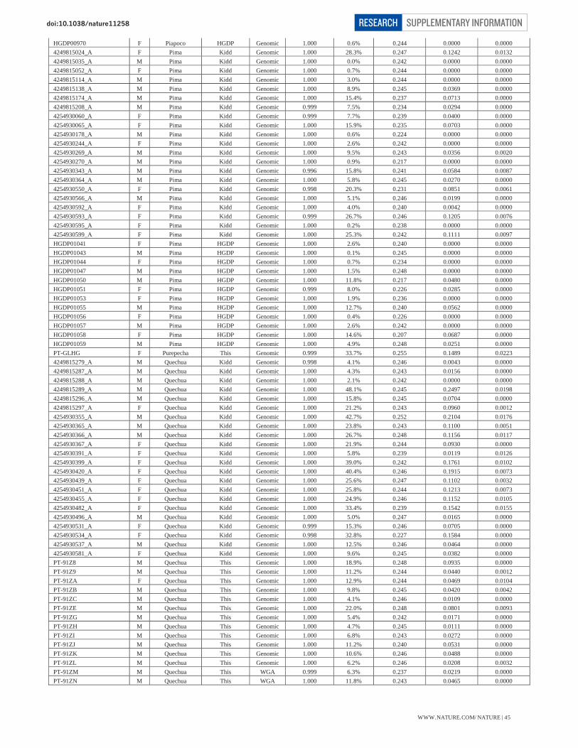
HGDP00970 F Piapoco HGDP Genomic 1.000 0.6% 0.244 0.0000 0.0000 4249815024_A F Pima Kidd Genomic 1.000 28.3% 0.247 0.1242 0.0132 4249815035_A M Pima Kidd Genomic 1.000 0.0% 0.242 0.0000 0.0000 4249815052_A F Pima Kidd Genomic 1.000 0.7% 0.244 0.0000 0.0000 4249815114_A M Pima Kidd Genomic 1.000 3.0% 0.244 0.0000 0.0000 4249815138_A M Pima Kidd Genomic 1.000 8.9% 0.245 0.0369 0.0000 4249815174_A M Pima Kidd Genomic 1.000 15.4% 0.237 0.0713 0.0000 4249815208_A M Pima Kidd Genomic 0.999 7.5% 0.234 0.0294 0.0000 4254930060_A F Pima Kidd Genomic 0.999 7.7% 0.239 0.0400 0.0000 4254930065_A F Pima Kidd Genomic 1.000 15.9% 0.235 0.0703 0.0000 4254930178_A M Pima Kidd Genomic 1.000 0.6% 0.224 0.0000 0.0000 4254930244_A F Pima Kidd Genomic 1.000 2.6% 0.242 0.0000 0.0000 4254930269_A M Pima Kidd Genomic 1.000 9.5% 0.243 0.0356 0.0020 4254930270_A M Pima Kidd Genomic 1.000 0.9% 0.217 0.0000 0.0000 4254930343_A M Pima Kidd Genomic 0.996 15.8% 0.241 0.0584 0.0087 4254930364_A M Pima Kidd Genomic 1.000 5.8% 0.245 0.0270 0.0000 4254930550_A F Pima Kidd Genomic 0.998 20.3% 0.231 0.0851 0.0061 4254930566_A M Pima Kidd Genomic 1.000 5.1% 0.246 0.0199 0.0000 4254930592_A F Pima Kidd Genomic 1.000 4.0% 0.240 0.0042 0.0000 4254930593_A F Pima Kidd Genomic 0.999 26.7% 0.246 0.1205 0.0076 4254930595_A F Pima Kidd Genomic 1.000 0.2% 0.238 0.0000 0.0000 4254930599_A F Pima Kidd Genomic 1.000 25.3% 0.242 0.1111 0.0097 HGDP01041 F Pima HGDP Genomic 1.000 2.6% 0.240 0.0000 0.0000 HGDP01043 M Pima HGDP Genomic 1.000 0.1% 0.245 0.0000 0.0000 HGDP01044 F Pima HGDP Genomic 1.000 0.7% 0.234 0.0000 0.0000 HGDP01047 M Pima HGDP Genomic 1.000 1.5% 0.248 0.0000 0.0000 HGDP01050 M Pima HGDP Genomic 1.000 11.8% 0.217 0.0480 0.0000 HGDP01051 F Pima HGDP Genomic 0.999 8.0% 0.226 0.0285 0.0000 HGDP01053 F Pima HGDP Genomic 1.000 1.9% 0.236 0.0000 0.0000 HGDP01055 M Pima HGDP Genomic 1.000 12.7% 0.240 0.0562 0.0000 HGDP01056 F Pima HGDP Genomic 1.000 0.4% 0.226 0.0000 0.0000 HGDP01057 M Pima HGDP Genomic 1.000 2.6% 0.242 0.0000 0.0000 HGDP01058 F Pima HGDP Genomic 1.000 14.6% 0.207 0.0687 0.0000 HGDP01059 M Pima HGDP Genomic 1.000 4.9% 0.248 0.0251 0.0000 PT-GLHG F Purepecha This Genomic 0.999 33.7% 0.255 0.1489 0.0223 4249815279_A M Quechua Kidd Genomic 0.998 4.1% 0.246 0.0043 0.0000 4249815287_A M Quechua Kidd Genomic 1.000 4.3% 0.243 0.0156 0.0000 4249815288_A M Quechua Kidd Genomic 1.000 2.1% 0.242 0.0000 0.0000 4249815289_A M Quechua Kidd Genomic 1.000 48.1% 0.245 0.2497 0.0198 4249815296_A M Quechua Kidd Genomic 1.000 15.8% 0.245 0.0704 0.0000 4249815297_A F Quechua Kidd Genomic 1.000 21.2% 0.243 0.0960 0.0012 4254930355_A M Quechua Kidd Genomic 1.000 42.7% 0.252 0.2104 0.0176 4254930365_A M Quechua Kidd Genomic 1.000 23.8% 0.243 0.1100 0.0051 4254930366_A M Quechua Kidd Genomic 1.000 26.7% 0.248 0.1156 0.0117 4254930367_A F Quechua Kidd Genomic 1.000 21.9% 0.244 0.0930 0.0000 4254930391_A F Quechua Kidd Genomic 1.000 5.8% 0.239 0.0119 0.0126 4254930399_A F Quechua Kidd Genomic 1.000 39.0% 0.242 0.1761 0.0102 4254930420_A F Quechua Kidd Genomic 1.000 40.4% 0.246 0.1915 0.0073 4254930439_A F Quechua Kidd Genomic 1.000 25.6% 0.247 0.1102 0.0032 4254930451_A F Quechua Kidd Genomic 1.000 25.8% 0.244 0.1213 0.0073 4254930455_A F Quechua Kidd Genomic 1.000 24.9% 0.246 0.1152 0.0105 4254930482_A F Quechua Kidd Genomic 1.000 33.4% 0.239 0.1542 0.0155 4254930496_A M Quechua Kidd Genomic 1.000 5.0% 0.247 0.0165 0.0000 4254930531_A F Quechua Kidd Genomic 0.999 15.3% 0.246 0.0705 0.0000 4254930534_A F Quechua Kidd Genomic 0.998 32.8% 0.227 0.1584 0.0000 4254930537_A M Quechua Kidd Genomic 1.000 12.5% 0.246 0.0464 0.0000 4254930581_A F Quechua Kidd Genomic 1.000 9.6% 0.245 0.0382 0.0000 PT-91Z8 M Quechua This Genomic 1.000 18.9% 0.248 0.0935 0.0000 PT-91Z9 M Quechua This Genomic 1.000 11.2% 0.244 0.0440 0.0012 PT-91ZA F Quechua This Genomic 1.000 12.9% 0.244 0.0469 0.0104 PT-91ZB M Quechua This Genomic 1.000 9.8% 0.245 0.0420 0.0042 PT-91ZC M Quechua This Genomic 1.000 4.1% 0.246 0.0109 0.0000 PT-91ZE M Quechua This Genomic 1.000 22.0% 0.248 0.0801 0.0093 PT-91ZG M Quechua This Genomic 1.000 5.4% 0.242 0.0171 0.0000 PT-91ZH M Quechua This Genomic 1.000 4.7% 0.245 0.0111 0.0000 PT-91ZI M Quechua This Genomic 1.000 6.8% 0.243 0.0272 0.0000 PT-91ZJ M Quechua This Genomic 1.000 11.2% 0.240 0.0531 0.0000 PT-91ZK M Quechua This Genomic 1.000 10.6% 0.246 0.0488 0.0000 PT-91ZL M Quechua This Genomic 1.000 6.2% 0.246 0.0208 0.0032 PT-91ZM M Quechua This WGA 0.999 6.3% 0.237 0.0219 0.0000 PT-91ZN M Quechua This WGA 1.000 11.8% 0.243 0.0465 0.0000



PT-91ZO M Quechua This Genomic 1.000 8.9% 0.241 0.0333 0.0000 PT-91ZP M Quechua This Genomic 1.000 46.0% 0.244 0.2180 0.0220 PT-91ZQ M Quechua This Genomic 1.000 7.2% 0.248 0.0301 0.0000 PT-91ZR M Quechua This WGA 1.000 5.9% 0.241 0.0208 0.0000 4256126001_A M Surui HGDP Genomic 1.000 0.0% 0.221 0.0000 0.0000 4256126002_A F Surui HGDP Genomic 1.000 0.0% 0.197 0.0000 0.0000 4256126004_A M Surui HGDP Genomic 1.000 0.0% 0.205 0.0000 0.0000 4256126007_A M Surui HGDP Genomic 1.000 0.0% 0.191 0.0000 0.0000 4256126036_A F Surui HGDP Genomic 1.000 0.0% 0.207 0.0000 0.0000 4256126086_A M Surui HGDP Genomic 1.000 0.0% 0.197 0.0000 0.0000 4256126171_A F Surui HGDP Genomic 1.000 0.0% 0.212 0.0000 0.0000 4256126172_A M Surui HGDP Genomic 1.000 0.0% 0.223 0.0000 0.0000 4256126173_A F Surui HGDP Genomic 1.000 0.0% 0.188 0.0000 0.0000 4256126183_A M Surui HGDP Genomic 1.000 0.0% 0.203 0.0000 0.0000 4256126202_A M Surui HGDP Genomic 1.000 0.0% 0.212 0.0000 0.0000 4256126311_A F Surui HGDP Genomic 1.000 0.0% 0.200 0.0000 0.0000 4256126312_A F Surui HGDP Genomic 1.000 0.0% 0.196 0.0000 0.0000 4256126330_A M Surui HGDP Genomic 0.999 0.0% 0.211 0.0000 0.0000 4256126341_A F Surui HGDP Genomic 1.000 0.0% 0.200 0.0000 0.0000 4256126376_A F Surui HGDP Genomic 1.000 0.0% 0.200 0.0000 0.0000 HGDP00832 F Surui HGDP Genomic 1.000 0.0% 0.196 0.0000 0.0000 HGDP00837 M Surui HGDP Genomic 1.000 0.0% 0.202 0.0000 0.0000 HGDP00838 F Surui HGDP Genomic 1.000 0.0% 0.223 0.0000 0.0000 HGDP00843 M Surui HGDP Genomic 1.000 0.0% 0.215 0.0000 0.0000 HGDP00845 M Surui HGDP Genomic 1.000 0.0% 0.208 0.0000 0.0000 HGDP00846 F Surui HGDP Genomic 1.000 0.0% 0.211 0.0000 0.0000 HGDP00849 M Surui HGDP Genomic 1.000 0.0% 0.210 0.0000 0.0000 HGDP00852 F Surui HGDP Genomic 1.000 0.0% 0.206 0.0000 0.0000 Tepehuano_10000_101700 M Tepehuano MGDP Genomic 1.000 9.8% 0.247 0.0379 0.0017 Tepehuano_10000_102700 F Tepehuano MGDP Genomic 0.999 5.3% 0.246 0.0162 0.0000 Tepehuano_10003_101703 M Tepehuano MGDP Genomic 0.998 7.0% 0.246 0.0283 0.0000 Tepehuano_10003_102703 F Tepehuano MGDP Genomic 0.999 21.0% 0.247 0.0867 0.0081 Tepehuano_10007_102807 F Tepehuano MGDP Genomic 1.000 11.5% 0.245 0.0469 0.0000 Tepehuano_10009_101709 M Tepehuano MGDP Genomic 1.000 16.4% 0.247 0.0631 0.0124 Tepehuano_10009_102709 F Tepehuano MGDP Genomic 1.000 7.7% 0.243 0.0323 0.0000 Tepehuano_10018_101718 M Tepehuano MGDP Genomic 1.000 17.5% 0.241 0.0697 0.0087 Tepehuano_10018_102718 F Tepehuano MGDP Genomic 0.997 19.3% 0.245 0.0831 0.0080 Tepehuano_10023_101723 M Tepehuano MGDP Genomic 1.000 6.5% 0.243 0.0220 0.0000 Tepehuano_10023_102723 F Tepehuano MGDP Genomic 1.000 8.6% 0.248 0.0319 0.0052 Tepehuano_10026_102726 F Tepehuano MGDP Genomic 1.000 1.0% 0.244 0.0000 0.0000 Tepehuano_10027_101727 M Tepehuano MGDP Genomic 1.000 5.6% 0.240 0.0218 0.0000 Tepehuano_10028_101728 M Tepehuano MGDP Genomic 1.000 4.4% 0.247 0.0108 0.0000 Tepehuano_10028_102728 F Tepehuano MGDP Genomic 0.999 5.2% 0.247 0.0188 0.0000 Tepehuano_10030_101730 M Tepehuano MGDP Genomic 1.000 9.8% 0.247 0.0380 0.0000 Tepehuano_10030_102730 F Tepehuano MGDP Genomic 0.999 13.5% 0.244 0.0595 0.0000 Tepehuano_10035_101735 M Tepehuano MGDP Genomic 0.987 10.6% 0.252 0.0405 0.0005 Tepehuano_10038_102738 F Tepehuano MGDP Genomic 0.999 5.6% 0.246 0.0188 0.0000 Tepehuano_10039_101739 M Tepehuano MGDP Genomic 0.999 19.7% 0.244 0.0939 0.0000 Tepehuano_10039_102739 F Tepehuano MGDP Genomic 0.999 9.2% 0.253 0.0315 0.0112 Tepehuano_10040_101740 M Tepehuano MGDP Genomic 1.000 1.5% 0.249 0.0000 0.0000 Tepehuano_10040_102740 F Tepehuano MGDP Genomic 0.999 5.0% 0.248 0.0131 0.0000 Tepehuano_10098_101798 M Tepehuano MGDP Genomic 1.000 3.5% 0.246 0.0061 0.0030 Tepehuano_10099_101799 M Tepehuano MGDP Genomic 1.000 11.6% 0.244 0.0566 0.0000 PT-918O M Teribe This WGA 0.998 3.3% 0.215 0.0000 0.0088 PT-918P M Teribe This WGA 0.999 0.1% 0.222 0.0000 0.0000 PT-918Q M Teribe This WGA 0.998 0.1% 0.214 0.0000 0.0000 PT-91CY F Ticuna This WGA 0.988 4.7% 0.217 0.0000 0.0000 PT-91CZ M Ticuna This Genomic 1.000 0.2% 0.213 0.0000 0.0000 PT-91D3 F Ticuna This Genomic 1.000 17.7% 0.245 0.0213 0.0577 PT-GLFP F Ticuna This Genomic 0.998 0.1% 0.220 0.0000 0.0000 PT-GLG2 F Ticuna This Genomic 0.999 2.4% 0.227 0.0000 0.0000 PT-GLGE F Ticuna This Genomic 0.996 3.1% 0.227 0.0000 0.0000 PT-GLFJ M Toba This Genomic 0.995 1.1% 0.243 0.0000 0.0000 PT-GLFV M Toba This Genomic 0.999 6.0% 0.242 0.0217 0.0000 PT-GLG8 M Toba This Genomic 0.997 7.9% 0.242 0.0237 0.0000 PT-GLH8 M Toba This Genomic 0.999 1.1% 0.245 0.0000 0.0000 PT-91DH M Waunana This WGA 0.993 0.1% 0.236 0.0000 0.0000 PT-91DI M Waunana This WGA 0.997 0.4% 0.235 0.0000 0.0000 PT-GLFL M Waunana This Genomic 0.961 3.6% 0.227 0.0000 0.0000 PT-91DL M Wayuu This WGA 1.000 3.3% 0.238 0.0060 0.0037 PT-91DQ M Wayuu This WGA 0.999 1.5% 0.236 0.0000 0.0000



PT-91DW M Wayuu This WGA 0.979 1.2% 0.226 0.0000 0.0000 PT-91DX M Wayuu This WGA 0.996 55.7% 0.236 0.1992 0.0992 PT-91E9 F Wayuu This WGA 0.986 73.1% 0.231 0.2212 0.1668 PT-91EF F Wayuu This WGA 0.977 25.5% 0.219 0.0740 0.0298 PT-9GS6 M Wayuu This Genomic 0.992 20.4% 0.234 0.0751 0.0158 PT-9GS8 M Wayuu This Genomic 0.997 8.1% 0.241 0.0138 0.0241 PT-9GS9 M Wayuu This Genomic 0.992 27.9% 0.237 0.1024 0.0127 PT-9GSB F Wayuu This Genomic 1.000 1.6% 0.236 0.0000 0.0000 PT-9GSC M Wayuu This Genomic 0.998 14.9% 0.238 0.0421 0.0338 westGreenland1 F WestGreenland Willerslev Genomic 1.000 50.6% 0.256 0.2173 0.0000 westGreenland11 F WestGreenland Willerslev Genomic 1.000 20.9% 0.252 0.0801 0.0000 westGreenland16 F WestGreenland Willerslev Genomic 1.000 17.9% 0.250 0.0556 0.0000 westGreenland2 F WestGreenland Willerslev Genomic 1.000 56.7% 0.251 0.2937 0.0000 westGreenland20 F WestGreenland Willerslev Genomic 1.000 37.9% 0.251 0.1578 0.0000 westGreenland5 F WestGreenland Willerslev Genomic 0.999 76.8% 0.246 0.4496 0.0000 westGreenland6 F WestGreenland Willerslev Genomic 1.000 76.2% 0.231 0.4594 0.0000 westGreenland9 F WestGreenland Willerslev Genomic 1.000 73.7% 0.239 0.4435 0.0000 PT-GLFH M Wichi This Genomic 1.000 25.7% 0.230 0.1181 0.0044 PT-GLFT F Wichi This Genomic 0.999 0.0% 0.216 0.0000 0.0000 PT-GLG6 F Wichi This Genomic 0.999 0.3% 0.225 0.0000 0.0000 PT-GLGI M Wichi This Genomic 0.999 0.1% 0.215 0.0000 0.0000 PT-GLGU M Wichi This Genomic 1.000 0.1% 0.219 0.0000 0.0000 PT-91YI F Yaghan This WGA 0.999 0.3% 0.215 0.0000 0.0000 PT-91YJ F Yaghan This WGA 1.000 53.4% 0.246 0.2393 0.0063 PT-91YL F Yaghan This WGA 0.998 53.5% 0.246 0.2544 0.0110 PT-91YM F Yaghan This WGA 0.988 32.2% 0.248 0.1308 0.0000 PT-912H F Yaqui This WGA 0.957 42.4% 0.224 0.1651 0.0118 PT-8ZVR F Zapotec1 This WGA 0.992 12.8% 0.247 0.0509 0.0038 PT-8ZVS F Zapotec1 This WGA 0.992 0.2% 0.244 0.0000 0.0000 PT-8ZVZ M Zapotec1 This WGA 0.965 2.4% 0.227 0.0000 0.0000 PT-9128 F Zapotec1 This WGA 0.983 23.8% 0.235 0.0997 0.0037 PT-913D M Zapotec1 This Genomic 0.994 13.7% 0.243 0.0645 0.0039 PT-913E F Zapotec1 This Genomic 0.997 43.7% 0.252 0.1690 0.0548 PT-913F F Zapotec1 This Genomic 0.999 18.2% 0.247 0.0852 0.0000 PT-913G F Zapotec1 This Genomic 1.000 15.4% 0.256 0.0681 0.0018 PT-913H F Zapotec1 This Genomic 1.000 20.7% 0.248 0.0895 0.0015 PT-913I F Zapotec1 This Genomic 1.000 16.8% 0.247 0.0711 0.0030 PT-913J F Zapotec1 This Genomic 0.990 19.1% 0.241 0.0895 0.0029 PT-913Q F Zapotec1 This Genomic 1.000 8.4% 0.247 0.0230 0.0100 PT-913R F Zapotec1 This Genomic 1.000 12.0% 0.249 0.0448 0.0084 PT-913S M Zapotec1 This Genomic 1.000 12.4% 0.252 0.0522 0.0000 PT-913U F Zapotec1 This Genomic 1.000 12.1% 0.253 0.0515 0.0000 PT-913V F Zapotec1 This Genomic 1.000 30.4% 0.256 0.1376 0.0000 PT-913W F Zapotec1 This Genomic 1.000 7.0% 0.254 0.0352 0.0000 PT-913X F Zapotec1 This Genomic 1.000 8.5% 0.250 0.0360 0.0000 PT-913Y F Zapotec1 This Genomic 1.000 24.0% 0.253 0.1233 0.0033 PT-913Z F Zapotec1 This Genomic 1.000 21.0% 0.249 0.0852 0.0056 PT-9141 F Zapotec1 This Genomic 1.000 8.6% 0.251 0.0233 0.0117 PT-9142 M Zapotec1 This Genomic 1.000 12.3% 0.249 0.0467 0.0000 Zapotec_20002_202602 F Zapotec2 MGDP Genomic 1.000 3.0% 0.247 0.0100 0.0000 Zapotec_20004_201604 M Zapotec2 MGDP Genomic 1.000 6.3% 0.245 0.0299 0.0000 Zapotec_20006_201606 M Zapotec2 MGDP Genomic 1.000 2.7% 0.248 0.0000 0.0000 Zapotec_20007_201607 M Zapotec2 MGDP Genomic 1.000 1.5% 0.254 0.0000 0.0000 Zapotec_20009_202609 F Zapotec2 MGDP Genomic 1.000 3.8% 0.250 0.0068 0.0000 Zapotec_20013_202513 F Zapotec2 MGDP Genomic 1.000 2.7% 0.250 0.0056 0.0000 Zapotec_20016_201516 M Zapotec2 MGDP Genomic 1.000 5.5% 0.247 0.0143 0.0000 Zapotec_20019_201519 M Zapotec2 MGDP Genomic 0.999 3.5% 0.244 0.0004 0.0000 Zapotec_20020_201520 M Zapotec2 MGDP Genomic 1.000 6.7% 0.240 0.0282 0.0000 Zapotec_20029_201529 M Zapotec2 MGDP Genomic 0.999 4.9% 0.252 0.0118 0.0071 Zapotec_20034_202534 F Zapotec2 MGDP Genomic 0.999 3.2% 0.249 0.0079 0.0000 Zapotec_20040_202540 F Zapotec2 MGDP Genomic 0.999 4.9% 0.250 0.0143 0.0000 Zapotec_20042_202542 F Zapotec2 MGDP Genomic 0.999 3.7% 0.251 0.0128 0.0000 Zapotec_20043_201543 M Zapotec2 MGDP Genomic 1.000 3.1% 0.250 0.0057 0.0000 Zapotec_20045_202545 F Zapotec2 MGDP Genomic 1.000 8.3% 0.242 0.0341 0.0000 Zapotec_20048_202548 F Zapotec2 MGDP Genomic 1.000 5.9% 0.240 0.0192 0.0000 Zapotec_20055_201555 M Zapotec2 MGDP Genomic 1.000 4.0% 0.243 0.0085 0.0000 Zapotec_20059_201559 M Zapotec2 MGDP Genomic 0.999 3.8% 0.242 0.0050 0.0000 Zapotec_20060_202560 F Zapotec2 MGDP Genomic 0.996 1.5% 0.249 0.0000 0.0000 Zapotec_20066_202566 F Zapotec2 MGDP Genomic 1.000 4.7% 0.239 0.0118 0.0000 Zapotec_20069_201569 M Zapotec2 MGDP Genomic 0.995 8.0% 0.244 0.0269 0.0000



Documents

7 6 2012 Supplementary material CORRECTED 2genetics.med.harvard.edu/reichlab/Reich_Lab/Publications...Chilote This 10 8 Karitiana HGDP/Kidd 34 13 Toba This 5 4 Chipewyan This 15 15