AD-A259 753 DTIC USAFETAC/PR-92/O0'lhhE*IIII I S ELECTE D

JAN 4193

ASPAMATMOSPHERIC SLANT PATH

ANALYSIS MODELStatistical Paired Differences Pilot Study

for Sample Size Determination

by

Capt Thomas H. ElioMr Charles R. Coffin

Major Lauraleen O'Connor

NOVEMBER 1992

O mm Approved for public release;Distribution Is unlimited.

REPRODUCED BYU.S. DEPARTMENT OF COMMERCE-NONATIONAL TECHNICAL

INFORMATION SERVICESPRINGFIELD, VA 22161

ENVIRONMENTAL TECHNICALAPPLICATIONS CENTER (USAFETAC)

Scott Air Force Base, Illinois, 62225-5116

92 12 _2£ l

REVIEW AND APPROVAL STATEMENT

USAFETAC/PR--9ZW05, ASPAM (Atmospheric Slant Path Analysis Model) Statistical PairedDifferences Pilot Study for Sample Siae Determination, November 1992, has been reviewed and isapproved for public release. There is no objection to unlimited distribution of this documentto the public at large, or by the Defense Technical Information Center (DTIC) to the NationalTechnical Information Service (NTIS).

ge't 7 ))A&AWALTER F. MIJLERChief, Simulations and Techniques Branch

FOR THE COMMANDER

WALTER 8.BURGý~Scientific and Technical InformationProgram Manager24 November 1992

ii0

REPORT DOCUMENTATION PAGE

2. Report Date: November 1992

3. Report True: Project Report

4. Title: ASPAM (Atmospheric Slant Path Analysis Model) Statistical Paired Differences PilotStudy for Sample Size Determination

6. Authors: Capt Thomas I- Elio, Mr Charles R. Coffin, and Maj Lauraleen O'Connor

7. Performinz Ormnization Names and Address: United States Air ForceEnvironmental Technical Applications Center (MT), Scott AFB, IL 62225-5116

8. Performing Organization Report Number. USAFETACVPR--92=05

12. Distribution/Availability Statement: Approved for public release; distribution isunliite&

13. Abstract: Describes methodology and results of a pilot study intended to determinethe required sample size for a statistically significant seasonal study of the differencesbetween ground truth (represented by upper-air soundings) and (1) Atmospheric Slant Path. Analysis Model (ASPAM) optimum interpolation vertical profiles (OIVPs) and (2) alternatevertical profiles. This study builds on earlier ASPAM studies, incorporating lessons learnedand user feedback. It found that a sample size of 50 observations was enough to determineif the differences between ground truth (upper-air soundings) and ASPAM vertical profileswere significant at the customer's confidence level.

14. Subject Terms: CLIMATOLOGY, ATMOSPHERE, PROFILES, UPPER-AIR,TEMPERATURE, MOISTURE, VERTICAL SOUNDINGS, SAMPLING, STATISTICS,STATISTICAL SAMPLING, SAMPLE SIZE, COMPUTERS, COMPUTING, COMPUTERMODELING,

15. Number of Pages: 42

17. Security Classification of Relport: Unclassified

18. Security Classification of this Paye: Unclassified19. Security Classification of Abstract: Unclassified Au.ahss1g For

20. Limitation of Abstract: UL 0tP 1" 0U Lur % mao n e ad [ 1Jt if Ieat!i

Standard Form 298Dl.st ri•b~lt in/Avwilablilty Codes

i Avell and/or

D•st Special

iii -LJ~D

PREFACE

This report documents a USAFETAC pilot study done for the Air Weather Service SpecialProjects Division (AWS/DOS). The study was initiated to determine the required sample sizefor a statistically significant seasonal study of the differences between ground truth(represented by upper-air soundings) and (1) Atmospheric Slant Path Analysis Model(ASPAM) optimum interpolation vertical profiles (OIVPs) and (2) alternate vertical profiles.

Specifically, AWS/DOS tasked USAFETAC to conduct a baseline ASPAM study that woulddetermine the spatial, seasonal, and temporal statistical variability of the temperature andmoisture optimum interpolation vertical profiles. The study only addresses the statisticalaccuracies of USAFETAC's version of the model.

In August 1990, USAFETAC's Special Projects Section (DOS) evaluated 112 cases fromvarious climatic regimes, seasons, and time of day. This study led to the discovery of severalminor ASPAM software problems. Other studies by the AWS Technology Division(AWS/XTX) postulated that HIRAS smoothing and/or limitations in the space-time resolutionof observations might degrade OIVP performance.

This study builds on earlier ASPAM studies, incorporating lessons learned and user feedback.It found that a sample size of 50 observations was enough to determine if the differencesbetween ground truth (upper-air soundings) and ASPAM vertical profiles were significant atthe customer-stated confidence level.

The authors wish to thank those who worked closely with us on this project. They includeMajor Harold Massie (AWS/DOS) for providing test guidance; Capt Jeff McCoy for McIDASsupport; the USAFETAC Point Analysis Team (Mr Mark Surmeier, Capts Greg Reding andDavid Martens, MSgt Richard Boyle, TSgts Heidi Tryon, Joan Bergmann and CatherineBird), the USAFETAC Database Administration Section (TSgt Dennis Murphy and MrsNancy Toon); AFGWCs special projects people (Capt Farrar and Capt Lunn); the AFGWCdatabase administrator (Capt Hanser); and the AFGWC HIRAS maintenance programmer(Capt Carlson). Finally, thanks to Mr Tom Kotz, USAFETAC/OL-A, for providing the datanecessary for a thorough statistical evaluation.

1

TABLE OF CONTENTS

Page1. INTRODUCTION .................................................. 11.1 ASPAM Background ............................................... 11.2 Why the Study Was Conducted ....................................... 11.3 How the Study Was Conducted ....................................... 2

2. PILOT STUDY STATISTICS ......................................... 32.1 Analysis Flow .................................................... 32.2 Statistical Sampling ............................................... 32.3 Population and Sample Size ......................................... 52.4 Statistical Approach ............................................... 62.5 Requirements and Development ...................................... 9

3. DETEMINING SAMPLE SIZE ...................................... 113.1 Objective ....................................................... 113.2 Paired Differences ............................................... 113.3 Simple Random Samples .......................................... 11

4. SUMMARY OF RESULTS AND CONCLUSIONS ........................ 124.1 Selecting the Sample Size .......................................... 124.2 Desired Sampling Error ........................................... 12S 4.3 Resultant Confidence ............................................. 134.4 Conclusions .................................................... 13

BIBLIOGRAPHY .................................................... 14

ACRINABS ........................................................ 15

APPENDIX A--Mean, Standard Deviation, Skewness, and Kurtosis ............ A-1

APPENDIX B--Mean Differences and Confidence Limits Sampling Error ........ B-1

APPENDIX C--Pilot Study Minimum and Maximum Sample Sizes ............. C-1

V

O 1. INTRODUCTION

1.1 ASPAM Background. AFGWC and In August 1990, USAFETAC's SpecialUSAFETAC provide detailed vertical Projects Section (DOS) evaluated 112atmospheric profiles to specified military ASPAM vertical profiles from variousagencies and Department of Defense (DoD) climatic regimes, seasons, and time of day.contractors. These profiles, called "point The evaluation led to the discovery ofanalyses," provide customers with the several minor software problems. Althoughmeteorological data they need to make there were too few samples used to achievedecisions with respect to atmospheric statistical significance, the study providedconditions at a specific place and time. The a better understanding of the model'scomputer model used to produce these point strengths and weaknesses, which included:analyses (or PAs) is called the "AtmosphericSlant Path Analysis Model," or "ASPAM." * The optimum interpolationThe model was recently enhanced to vertical profile (OIVP) scheme did notaccommodate new or improved use (or may have misused) RAOBmeteorological databases and improved data.techniques, such as:

• OIVP moisture errors can (at* The New Upper Air Validator times) significantly exceed RAOB(NUAV). instrument errors.

a The Real-time Nephanalysis * The use of an eighth-mesh terrain(RTNEPH) cloud database. database contributed to large densitySerrors inareas ofcomplex tran

* Finer resolution data fields in the

High-Resolution Analysis System Other studies by the AWS Technology(HIRAS). Division (XTX) postulated that HIRAS

smoothing, and/or limitations in the space-* More sophisticated mathematical time resolution of observations, might alsotechniques, such as statistical degrade OIVP performance.optimum interpolation, which weightsvarious observations not only by their 1.2 Why the Study Was Conducted. Asdistance from the point of interest, requested by the Air Weather Servicebut by the statistical accuracy of the Directorate of Operations, Special Projectsdifferent types of data used. Division (AWS/DOS), USAFETAC evaluated

the Atmospheric Slant Path Analysis Modelo Alternate vertical profiles, which (ASPAM) to determine the seasonalprovide temperature profiles one statistical variance of the tempera-standard deviation warmer and ture/noisture optimum interpolation verticalmoisture profiles one standard profiles (OIVPs). This study builds upondeviation drier than the "best" several earlier ASPAM studies,temperature and moisture profiles. incorporating lessons learned and user

feedback. The study had two mainpurposes:

S

* Satisfy point analysis customer regions. The study describes sample sizerequirements for a statistically calculation for ASPAM differences fromsignificant baseline analysis of the ground-truth.ASPAM temperature and moistureOIVP and alternate profiles by Radiosonde observations (RAOBs), used asclimatic regions, season and ground truth, were denied from the Airatmospheric level. Force Global Weather Central's (AFGWC's)

parallel High Resolution Analysis System* Provide data for use in (HIRAS) database. ASPAM profiles weredetermining if modifications for the subsequently analyzed at the denied RAOBASPAM code were required. locations, then compared with those RAOBs.

1.3 How the Study was Conducted. Finally, analysts determined the number ofUSAFETAC measured differences from the observations needed for a statistically validsurface to 100,000 feet for the polar/arctic, variance study of ASPAM temperattre andmid-latitude, and moist tropical climatic moisture accuracy.

2e

P 2. PILOT STUDY STATISTICS

2.1 Analysis Flow. The pilot study an estimate made from a smaller sampleconsisted of separate sample size drawn at random. As the sample sizecalculations for each region (arctic, mid- becomes larger, the sample estimate differslatitude, and moist tropics) of the mean less and less from the expected value. It iserror, standard deviation, examined necessary to determine a degree ofdifferences between ASPAM's RAOBVP assurance that the sample selection isanalysis (ground truth) and OIVP within the range stated.temperature and moisture profiles.

This assurance is called the "confidenceThe mean and standard deviation of the level." If a large number of samples aredifferences for temperature and moisture chosen from a given field (population), theywere calculated from the surface to 100,000 will tend to cluster around a more realisticfeet above ground level in 1,000-foot value of the field. Some of the samples,increments to 10,000 feet and every 5,000 however, will tend to be extreme and liefeet thereafter. The sample sizes were outside the limits of this cluster. Bycalculated using these results. statistical methods, it is possible to measure

the percentage of time a sample of a given2.2 Statistical Sampling. A statistical size would result in a condition that issampling plan constitutes three distinct within the stated range. The confidenceparts, all accomplished using strict level is usually expressed as a percentage;statistical techniques: values of 95%, 99% and 99.9% reflect very

high levels of assurance and meet most* Calculation of sample size using requirements.sample errors.

It can be shown that, for a particular* Selection of the sample. sample size, the wider the margin of

precision, the more assurance (or confidence)* Evaluation of the results. the sample will fall within it. Conversely,

the narrower the margin, the smaller theSampling error (or " precision') is how degree of assurance. Therefore, theclosely the result from a sample duplicates precision or confidence level, or both, can bethe result that can be obtained from the increased by increasing the sample size.complete population (Hansen et al., 1953). Our goal in this study was to determine theAnother way of looking at precision is how sample size that would result in the desiredclose the mean of randomly selected samples level of assurance.are to each other. Usually, the precision isstated as a value added to and subtracted Confidence intervals can also provide a testfrom the sample result. The population's of significance. If zero is within thecharacteristics are expected to lie confidence interval, then we say that thesomewhere between these limits. It's population mean difference is statisticallypossible to estimate the sampling error that equal to zero. If zero is outside thewill result from the use of a particular confidence intervals, then we can say thatsample size. If the number of items from the population mean difference iswhich to choose is limited, choosing more statistically not equal to zero (Law anditems will result in less risk than in using Kelton, 1991). That is, if a sample mean

p3

difference is statistically equal to zero, then well enough for practical applications whenthe same is implied for the entire samples come from non-normal populations.population. For this study, a zero meandifference implies the RAOBVP and OIVP Even when the distribution of a populationparameter values are not statistically is far from normal, the samplingdifferent; thus, the OIVP approximates the distribution of the mean approaches theground truth RAOBVP reasonably well. normal distribution as the sample size

increases (i.e., as it approaches infinity).Confidence intervals are based on randomsample means and standard errors. The yrandom sample mean is used to measure acentral value in the population oftemperature or humidity differences. Thesample standard deviation measures the 68%

scatter or spread in a series of differencesaround the sample mean. The standarderror is the standard deviation of adistribution of random sample means; it 95%measures the spread of a series of randomsample ans. Standard errors are used to thai 9make inm.,- ences about the likelihood that m : 99%

the popuidtion mean difference lies within -4o -3o -2a -1a AI 10 2a 3a 4a

the specified interval or range of differences.Figure 1. The Normal Distribution and the

The greatest advantage of using a statistical Empirical Rule from Schlotzhauer andtechnique to decide on a sampling plan is its Littel, 1987.ability to measure the reliability and degreeof assurance that can be placed on the Although we cannot know the wAt valhn ofresults. The second most important the error of the estimate of the mean, fromadva ý.e of statistical sampling is the the empirical rule for the normalassu -. that the test will objectively bring distribution shown in Figure 1 we can say:to lignii a reasonable cross-section of thefield being examined. If the sample is * 68% of the values are within oneselected according to proper statistical standard deviation of the mean.standards, results are justified by using thestatistical tables appropriate for the * 95% of the values are within twodistribution (Hill, Roth, and Arkin, 1979). standard deviations of the mean.

In many practical sampling problems, we e More than 99% of the values arecan assume the values in a dataset are a within three standard deviation,. ofsample from a normal distribution since the mean (Schlotzhauer and Littel,large classes of distributions approximate 1987).the normal distribution. This fact has greatpractical importance since it is relatively Skewness and kurtosis values are known aseasy mathematically to work with the "shape" statisti- mnd can be used asnormal distribution. Some results may hold measures of d.- - ture from normality.

"Skewness" mear, lack of data symmetry

4

about the mean. "Kurtosis" describes the where X is the mean, x, the number ofheaviness of the tails of a distribution, individual observations, and n is the total

sample size. The mean doesn't alwaysPositive skewness values indicate that the constitute the "typical" value for someprincipal part of the distribution is meteorological elements. For example, aconcentrated on the left side of the mean temperature is more representativedistribution mean, with a longer tail to the than mean daily rainfall since rainfall has aright. Negative skewness occurs when the greater tendency for extreme occurrencesprincipal part of a distribution is over short periods of time.concentrated on the right side of thedistribution mean, with a longer tail to the The mode, defined as the most probableleft. When the absolute value of skewness value of a variable, is not influenced byis greater than 1.0, the distribution is highly extremes at all.Lkewed; when it is between 0.5 and 1.0, thedistribution is moderately skewed, and when The median, the halfway point in ait is between 0.0 and 0.5, the distribution is frequency distribution, is influenced by thenearly symmetric. Skewness values can be number of observations, but not by the valueuseful in determining the type of of extreme members.distribution. A normal distribution has askewness value of about zero. Once the mean is determined, the degree of

variability is calculated using the standardExtremely non-normal distributions may deviation. The standard deviationhave large positive or negative kurtosisvalues, while nearly normal distributionshave kurtosis values close to zero. Kurtosis $ n__ (2)is positive if the tails are heavier than for a nnormal distribution and negative if the tailsare lighter than for a normal distribution. places emphasis on large deviations from

the mean (Panofsky and Brier, 1968).2.3 Population and Sample Size. Todetermine the sample size, the behavior of A t-test can be used to determine thethe data must be summarized by departure of a sample mean (i) from thedetermining the values of the variables that true mean, /J. The student-t value can belie near the middle of a frequency computed by the following (Snedecor anddistribution. Three measures of central Cochran, 1989):tendency (means, medians, and modes) arecommonly used to summarize statistical t- - (3)informat-',)n. The mean is obtained by the Saddition of all the observations in a sampleand division by the number of cases in the where )E is the sample mean n is the samplesample. The mean is defined as size, and e is the standard deviation of the

sample.

x(1) The confidence intervals can be used ton1 assess the accuracy of the computed sample

mean as an estimate of the populationmean. The confidence interval for the true

5

mean difference of paired observations of the confid, :e interval reflects sample(between RAOBVP and OIVP values, for size. Althougi large samples decrease thethis study) is given by Snedecor and size of the confidence interval, a smallCochran, 1989: sample might also provide adequate

information. According to Arkin (1974) andHansen, Hurwitz, and Madow (1953), the

-* ts3 (4) standard deviation can be determined froma random sample of 50 observations.

where d is the sample mean difference, n is Hansen, et al. (1953) states that if a simplethe sample size, t is the t-test table value, random sample is drawn from a populationand ad is the standard deviation of the that is approximated by the normaldifferences divided by the square root of the distribution, then 50 observations aresample size. enough to yield a reasonably reliable

estimate of the standard error of a mean.The 900/6, 95%, and 99% confidenceintervals for paired observations in this 2.4 Statistical Approach. Two approachesstudy were estimated using the normal for calculating the sample size weredistribution and Chebyshev's inequality. considered for the ASPAM pilot study:The normal approximation is usually usedwhen the sample size is greater than 30; The first, the simple random sample design,however, even if the population is not considered the mean standard deviation andnormally distributed, the central limit customer accuracy requirements. The ratiotheorem states that the sampling between customer accuracy requirements,distribution of the mean approaches a also referred to as sampling error (e.g.,normal distribution when the random temperature accurate to 20, 40, and 60 C),sample size is increased; that is, as the and the standard deviation was found. Thesample size (n) approaches infinity, ratio was used with the 99, 95, and 90Chebyshev's inequality can also be used to percent confidence limits to obtain thedete.mine confidence limits of the estimated sample size for the populationpopulation mean; it is very conservative mean differences based on winter 1992 data.and can be applied to any type of For example:distribution.

SE= - 1- (5)The skewness and kurtosis values given can Nbe used to determine an adjusted t value indefining the confidence interval. Althoughskewness and kurtosis computations should where SE is the sampling error (or customeronly be applied to larger samples, they can defined accuracy), t is the Student's t-testalso be informative in small samples. statistic value at a given confidence level, s

is an approximation of the standardA 95% confidence interval for an extremely deviation for the population of the pairedlarge population based on the normal differences, n is the required sample size,distribution (or Chebyshev's inequality for a and N is the population size for eachnon-normal distribution) means that we are stratum (region). As giv , 'y Arkin (1974),95% confident that the random interval will we can calculate the desired sample size bybe chosen so that .- happens tc )ntain the solving for sample size n:true population mean difference. The range

6

St2 2 1 (6)

N t 2 N n (9)

where [1+11N(A)JI-s (7)j

R SEAs a first approximation we can estimatethe sample size using

(o 2 tilO)

The table shows how the sample size varieswith the ratio (R) and the confidence levels, where n. is the sample size estimate. If

n/n is appreciable (not negligible) we- - -compute

Sample Confidence

n R N t Level n.

9090 0.02 20,000 * 2.58 99%l(n, (11)

6489 0.02 20,000 * 1.96 95%

228 0.17 20.000 * 2.58 99%

133 0.17 20,000 * 1.96 95% For example, for the following conditions,P =-and keeping within a 10% sampling error'.The second approach was a simple randomsample design that considered the standard Pilot sample mean (X) ... 3.50deviation and sample mean at different Population size, (NV) .... 2,500confidence levels. The value is calculated Pilot sample size .......... 20

Standard Deviation (s) .... 0.7nt _ (8) Epsilon (6) ............ 0.10ti•= N 99.730/6 Confidence level (t)+ 3.00

The sample size estimate is:whereas N, n t, s are as previously defined, (3A.V (9X.49) 4.41

e is the value set by the investigator; that n, .. )7X92 ... 36(12)

is, the sample mean estimate (X) should notdiffer from the unknown population mean(p) by more than ep. The product (epu) is Then, solving for nessentially the sampling error stated in our 3 36first approach, but expressed in terms of n = 36 1 ÷ 0.0144 = 35.48 (13)X-p, called "sampling error" or "precision," 1 ÷ 10which is the difference between a "sample" 2500result and the result from a 100%/6 check (thewhole population). Solving for n gives In other words, given our example

conditions, a sample size of 36 is needed tohave a statistically significant test.

P7

*0 ct

EV

CU

>00

CL

CC

CC0S

o Im 0 0 az v z

O0

. 2.5 Requirements and Development. This on 13 January 1992.study resulted in the determination of theminimum sample size needed at three * Enough data was denied (17confidence intervals (99, 95, and 90%). This observations times 2 cycles a day = 34was accomplished in the following steps: observations a day) to ensure that 50

observations from each region couldSTEP 1. AWS/DOS and USAFETAC/DOS be selected randomly. Denial beganselected the ground-truth upper-air stations 18 January and was terminated on 10shown in Figure 2. None of these were on February 1992.the "blacklists" of the High ResolutionAnalysis System (HIRAS) or the European STEP 3. AFGWC shipped the OOZ, 06Z,Center for Medium-range Weather 12Z, and 18Z HIRAS data, HIRAS errorForecasting (ECMWF)--that is, none of them fields, and denied observations for 18had a known recent history of poor data. January-10 February 1992 on the GlobalThey were selected from the Arctic (WMO ETAC Operational Network (GEON) toBlocks 70, 25, and 24), the mid-latitudes USAFETAC/OL-A for QC and reformatting(WMO Blocks 9, 10, 11, and 12), and the into the USAFETAC database format.tropics (WMO Blocks 98 and 48). Selectionswere made on the basis of high data density. STEP 4. OL-A shipped the HIRAS data (onStations chosen also showed good reporting GEON) to USAFETAC. USAFETAC beganfrequency at OOZ and 12Z from 1 to 15 receiving data-denied HIRAS and RAOBNovember 1991, as shown by the number of data from OL-A via GEON on 19 Januaryobservations in the USAFETAC upper-air and stored it out to Direct Access Storagedatabase; there were at least a dozen OOZ Devices (DASD) to prepare for ASPAMand 12Z upper-air soundings for each analysis.station.

STEP 5. USAFETAC/SYT analysts randomlySTEP 2. AFGWC denied the selected selected 50 vertical profiles per region byground truth observations from the non- date and time, for a total of 150 events.production HIRAS cycles from 18 January to10 February 1992. AFGWC imposes a limit STEP 6. USAFETAC/DOS analystsof 100 observations denied in one cycle, produced a point analysis (PA) for eachThis limit (documented in the HIRAS event using the OIVP option of ASPAM andmaintenance code) insures no degradation in the data-denied HIRAS fields. Ground-truththe analysis. Of the 100 observations, 83 profiles were produced by specifying theare currently used as being from RAOBVP option of ASPAM, using only the"blacklisted" stations. This left 17 denied RAOB as input. This put the groundobservations per cycle that could be used for truth in the same format as the pointtest stations. The following steps were used analyses.to run the off-line HIRAS between 18January and 10 February 1992: STEP 7. USAFETAC/DOS analysts

performed manual quality control on each* A parallel, non-production version ASPAM RAOBVP and OIVP they hadof HIRAS ran for 72 hours to produced. They then used the Man-eliminate any contamination by the Computer Interactive Data Access Systemstations whose observations were (McIDAS) to locate inconsistencies in thedenied. AFGWC started this process data.

9

STEP 8. ASPAM OIVP and RAOBVP 0 Using sampling errors of 1° forground truth analyses were used to conduct temperature and 0.05 g/m8 of thea paired difference statistical analysis to highest RAOBVP and OIVP valuesfind the required sample size for each (based on customer accuracyregion. The analysis also determined the requirements stated in thedifference means, mean sampling error, and USAFETAC/ECS (now DOS) Pointconfidence limits in the two ways stated Analysis Accuracy Study, Augustearlier in this chapter, that is: 1990).

a Inspecting a sample size of 50 usedto determine sample size for full test.

10

O 3. DETERMINING SAMPLE SIZE.

3.1 Objective. The appropriate sample size from 35,000 to 50,000 feet, the observationfor each of the three regions was determined mean differences are very near zero andusing the desired conildence interval, kurtosis values are extremely high,standard deviation, and allowable sampling indicating deviation from a normalerror. We examined the 95% and 99% distribution. As the kurtosis valueconfidence intervals for the paired increases, the size of the sample necessarydifferences, allowing sampling errors of 10 C to place confidence in our estimated samplefor temperature and 5% for humidity. These standard deviation increases. See thesampling errors were based on customer minimum and maximum columns inrequirements stated in the ASPAM accuracy Appendix A-3 for humidity at the surfacestudy conducted by USAFETAC/ECS (now and between the 30,000 to 50,000 foot levels.DOS) in 1990. The standard deviation ofthe differences between the RAOBVP According to Law and Kelton (1991), theground truth and the OIVP is based on 59, t-test can hold its own against troublesome52, and 53 sample size differences from skewness, especially when we deal witharctic/polar, mid-latitude, and moist tropics, paired differences, assuming that therespectively, ground-truth RAOBVP and OIVP

distributions are skewed in the same3.2 Paired Differences. The t-test can be direction (as they are in this test--at leastused to test the null hypothesis that the most of the time). If ground truth and OIVPpopulation mean of OIVP-RAOBVP paired distribution skewness values are frequentlydifferences is equal to zero (Panofsky and in opposite directions, we should use a moreBrier, 1968). Temperature differences and conservative technique; see 3.3.humidity differences were calculated bysubtracting OIVP data values from 3.3 Simple Random Samples. The tabularRAOBVP ground truth data values. The values in Appendices, C-2, C-3, and C-4mean values of the paired differences were represent the desired sampling size based onbased on random sample sizes given in 3.1. an optimum (idealistic) sampling error ofThe mean differences at heights from the 10 C for temperature and a desired samplingsurface to 100,000 feet (HTIK.FT) above error of 5%/6 of the highest RAOBVPground level for temperature (* C), and humidity value and 5% of the highest OIVPabsolute humidity (g/m), are given in hunmidity value. The sample sizes in C-5Appendix A. The standard error of the and C-6 were calculated for two cases: (1)differences are also given, sample mean differences were assumed to

be normally distributed, and (2) sampleThe tabulated values in Appendix A show mean differences were assumed to be notmoderate skewness for a number of normally distributed. Because Case 2 usestemperature differences except near the the conservative Chebyshev's inequality tosurface and at levels near the tropopause determine sample size, the resultant large(100,000 feet). Kurtosis values for humidity sample sizes can be applied to any type ofdifferences are low in a number of cases; but population other than normal.

4. SUMMARY OF RESULTS AND CONCLUSIONS.

4.1 Selecting the Sample Size. In humidity (0.168 &/mn) are too large to becomputing confidence limits, it is common to practical for the tiae constraints imposed onselect a reasonably normal sample size large this study.enough to be able to make assumptionsabout a sampling distribution. The problem Note: Humidity amounts decreasewith gathering a large random sample is exponentially in the vertical;that it is not always practical, especially therefore, the sampling errors forwhen we consider the amount of time it humidity shown in C-1 through C4takes to collect HIRAS data and run are significant only from the surfaceASPAM products. One way to overcome to 300 mb (moist levels). The amountthese limitations is to recognize the data of humidity in the upper tropospheredistortion in the random sample; that is, (above 300 mb) is negligible; thisinspect the skewness and kurtosis values, study does not attempt to measure

sampling errors at these heights.4.2 Desired Sampling Error. The skewnessand kurtosis values shown in Appendices We looked at errors we would have toA-2 through A-7 indicate that temperature tolerate if we use a sample size of 50 for theand 'unidity differences do not yield a full baseline study. Appendices C-5 (basednorm: listribution in our test: however, on population size for a season) and C-6even Laough the two datasets (such as (based on a very large population sizeRAOBVP and OIVP values) might be far approaching infinity) show the samplingfrom being normally distributed, the errors for the sample size of 50 for eachdistribution of the differences (RAOBVP- region. Note that in C-6 the sampling errorOIVP) will be approximately normal (Sachs, for a very large population is very similar to1984). Even so, our inclination is to lean our test using the seasonal population size.toward relying on the more conservative This indicates that using a seasonally sized95% confidence level for the Chebyshev population is sufficient, where "seasonalinequality. population" is defined as:

Appendices C-2 and C-4 are useful if we e6 denied stations/region x 3 monthswish to maintain the desired sampling error e3 months/season x 30 days/monthat 10 C for temperature and 5% of absolute e2 observatione/day = 1,080humidity at minimum and maximumstandard deviation. In C-2, for example, Sampling errors of 2.9, 4.2, and 1.90 C forassuming the minimum standard deviation the arctic, mid-latitude, and moist tropicof 1.53090 C, we need at least 9 to 10 regions, respectively (shown in C-5 for aobservations to be certain that the 95% sample size of 50), coincide with maximumnormal confidence interval contains the true standard deviation of the mean differencesmean difference. However, we need a for each region. Note that the samplingsample size of least 45 to 47 observations to errors are within 20 C of the inri - -mentbe certain that the 95% Chebyshev's error estimates (MGRCC, Document J3-87),conficnance interval (non-normal) contains which vary linearly with altitude fromthe true mean difference. The minimum 0.40 C at the surface to 1.80 C at 30required sample size at the 99%/ confidence kilometers.levels for 10 C for temperature and 5%

12

O 4.3 Resultant Confidence. No matter what on Chebyshev's inequality would makethe sample size used, one can correct for reasonable inferences about the populationdata distortion. In order to use a small mean differences for the three regions.sample of data drawn from a non-normaldistribution (such as the sample size of 50 4.4 Conclusions. A sample of 50per region per season used for this study), observations is enough for a statisticallywe must adjust the t values in the valid variance study of ASPAM temperatureconfidence intervals by using either the and moisture accuracy, provided theskewness and kurtosis values or customer can accept the sampling errorsChebyshev's inequality. Appendices B-2 given in Appendices C-5 and C-6 (95%through B-7 show that the confidence confidence assuming Chebyshev's inequal-interval contains zero, indicating that the ity). Sampling errors are based on hepopulation mean difference is statistically inimum and maximum standard deviationequal to zero. This is most evident in the for temperature and humidity given in99% confidence limits. Appendices C-2, C-3, and C-4 for each

region. If the length of the confidenceBy adjusting the t values at the 95% level, interval for the mean differences is notthe skewness and kurtosis values fall within small enough to meet customer require-the range of the t values based on ments, a larger sample size will beChebyshev's inequality at the 95% necessary. Customer requirements willconfidence level. We therefore determined determine if a sample size of 50 isthat using the 95% confidence interval based acceptable for future tests.

13

BIBLIOGRAPHY

Arkin, H., Handbook of Sampling for Auditing and Accounting, McGraw Hill, 1974.

Arkin, H., Sampling Methods for the Auditor, An Advanced Treatment, McGraw Hill,New York, 1982.

Downing, D. and Clark, J., Statissis, the Easy Way, Barron's Educational Series, Inc., 1983.

Hansen, M., Hurwitz, W., and Madow, W., Sample Survey Methods and Theory,John Wiley, 1953.

Hill, H. P., Roth, J. L., and Arkin, A., Sampling in Auditing, A Simplified Guide andStatistical Tables, Robert E. Krieger, Huntington, New York, 1979.

Law, A. M. and Kelton, W. D., Simulation Modeling and Analysis, Second Edition,McGraw Hill, 1991.

Meteorological Data Error Estimates, Meteorological Group Range Commanders Council(MGRCC), Secretariate Range Commanders' Council, White Sands Missile Range,New Mexico, Document 353-87.

Panofsky, H. A. and G.W. Brier, Some Applications of Statistics to Meteorology,The Pennsylvania State University, University Park, Pa, 1968.

Sachs, Lothar, Applied Statistics, A Handbook of Techniques, Second Edition, Springer-Verlag, 1984.

Schlotzhauer, S.D. and R.C. Littel, SAS System for Elementary Statistical Analysis, SAS Institute Inc.,Cary, NC, 1987.

Snedecor, G. W. and Cochran W. G., Statistical Methods, Iowa State UniversityPress/AMES, 1989.

Surmeier, M. T., IPAM Baseline Plan and Concept of Operations, United States Air ForceTechnical Applications Center, Scott Air Force Base, 11, 28 Oct 1991.

Surmeier, M. T., et al., Point Analysis Accuracy, A Detailed Study of PAs Created using theOld PA Model and IPAM, USAF Environment Technical Applications Center, Scott AirForce Base, II, Aug 1990.

S14

ACRINABS

ASPAM Atmospheric Slant Path Analysis Model

AFGWC Air Force Global Weather Central

ECMWF European Center for Medium-range Weather Forecasting

HIRAS High Resolution Analysis System

IPAM Improved Point Analysis Model

MAX Maximum

mb Millibar

McIDAS Man Computer Interactive Data Access System

MN Minimum

NUAV New Upper Air Validator

OIVP Optimum Interpolation Vertical Profile

O PA Point Analysis

RAOB Radiosonde Observation

RAOBVP RAOB-based Vertical Profile

RTNEPH Real-time Nephanalysis

STD Standard Deviation

SE Sampling Error

USAFETAC United States Air Force Environmental Technical Applications Center

WMO World Meteorology Organization

15

Appendix A

MEAN, STANDARD DEVIATION, SKEWNESS, AND KURTOSIS

A-1

ARCTIC/POLAROIVP-RAOBVP TEMPERATURE DIFFERENCES STATISTICS

07 07 9nDITUC DZl1PUUCZ SINDoT.1KFT 9 MOs D 1iJ oCr Ur lhBVEZS S •• •Skewness Kurtosis

1 $9 -0.6983051 4.637S340 -21.0000000 7.0000000 0.6037SSs -1.6140773 S.6328558

2 59 -0.3389831 4.293S805 -12.0000000 6.0000000 0.559766 -1.0020733 1.1316117

3 S9 0.8135593 3.2459S17 -7.0000000 13.0000000 0.4ZZS348 0.7460125 Z.6S81147'

4 59 1.1V14949 3.0439024 -6.0000000 10.0000000 0.3962RZ3 0.3252444 0.6300"Z

S c9 1.1355932 2.3668517 -5.3000000 6.0000000 0.306137q -0.0946434 0.3797406

& 59 3.83050o5 Z.2904544 -5.3000000 5.0000000 0.2982048 -0.12322?5 -0.1238945

7 59 0.359JZZ 2.Z496184 -6.0000000 o.0000000 0.2T29754 -0.5472111 0.69412SO

1: 9 0.3350547 Z.0:65269 -S.0000000 S.0000000 0.2716427 -0.41269S4 0.S049764

1 .99 0 2.0444250 -6.0000000 3.0030000 0.2713690 -0.8394599 0.4361726

12 %9 -3.01694Q2 1.4050541 -S.0000000 4.0030000 C.235Q019 -C.3197849 0.5584405

14 59 -0.0334983 1.5309013 -4.0000000 4.0000000 0.1993064 -0.0307100 0.9309345

16 -9 -0.0331943 1.5753062 -4.C000000 3.0011000 0.20S0874 -0.212075 -O.2764**Z

is 59 -0.1864407 1.736769S -5.0000000 4.0000000 0.2260•60 -0.255742 0.3516213

20 S9 -0.0677966 1.4723241 -3.0000000 4.0000000 0.11716823 -0.0137439 -0.1265"?

25 59 -0.1166441 1.7328942 -4.0200000 5.0000000 0.2256036 0.1809351 0.349.451

30 59 0.4745763 2.3514921 -6.0000000 5.0000000 0.3061362 -0.056975 -0.0094ZZ9

35 59 0.6440678 1.7196903 -4.0000000 6. 000000 0.2234846 0.3046434 1.9614620

40 59 -0.2ZO3390 1.2327121 -3.0000i00 3.0000000 0.1604854 0.0442263 0.2326Z96

45 59 -0.406779? 1.2473213 -4.0000000 3.0000000 0.1623577 0.11119S4 0.5705896

so S9 -0.7280136 1.6170443 -4.0000000 3.0000000 G.210S218 -n.0023716 -0.49552s5

60 %9 -0.uoo0475 1.6127053 -4.0000000 4.0000000 0.2S39963 -0.0679994 0.1666251

70 59 -0.3725814 2.S723646 -9.0000000 7.0000000 0.3346969 -0.'2ZZS30 ZZ414?7Z

80 59 -1.135932 3.5304470 -13.0000000 7.0030000 0.45962S1 -0.78164LT ZS.713273

90 59 -1a711864 3.9515624 -18.0000000 9.0000000 0.S14*496 -1.S213SIS 5.7897.00

U') 5q -0.6271146 4.1690S93 -11.0000000 14.0000000 0.S553691 0.%191422 1.940946

S$C Sy -3.4406760 S.1537438 -19.000000 6.0030000 0.6709603 -0.4APST54 0.7713737

A-2

ARCTIC/POLAROIVP-RAOBVP ABSOLUTE HUMIDITY DIFFERENCES STATISITCS

STA-40ANNEl OEV4ATI 111mN•I01 O1 DUThPI=lZ uDuZIc SWDA

JTltpF N 03s DhTTUU6IES DoIF.EUIcu UW ]am m uaollta Skemness Kurtosis

1 59 0.0224441 0.3313587 -1.1741000 1.1390000 0.0431392 0.1932530 4.4106435

2 %9 0.0110000 0.3373403 -0.9341000 1.1730000 0.0439160 0.1614716 2.47962L0

3 59 0.0666747 0.3191245 -0.6483000 1.z130000 0.0415465 0.8236910 2.4080997

4 59 0.076352S 0.3466425 -0.7129000 1.1356000 0.C451290 0.8739584 1.9831016

5 59 0.0061119 U.3146265 -1.1300000 0.7498000 0.0409609 -0.872*460 2.1165719

3 59 0.31616S8 0.3254250 -0.9950000 0).905000 n.042k108 3.1045911 1.774923Z

7 59 -0.0101739 0.32t9873 -1.1650000 0.9596000 r.c419192 -0.4J?0169 2.49'4790

3 59 -0.0337985 0.23S3434 -1.1143000 0.765000 O.0171485 -0.73642&2 3.1326631

1) 59 -0-'6iM1217 0.2254849 -C.8276000 0.2877000 ft.0Z9i5$6 -1.2.03449 2.9852650

12 S9 -O.Z,542954 0.1714451 -0.5421700 C.3724000 n.0223202 -(0.60R3362 2.1277226

14 99 -0.014P475 0.1069915 -0.3724000 0.3782000 f.0141495 0.511436' 3.7314604

1i 59 -0.31442q5 0.06S4667 -0.1854000 0.1938000 0.0089136 0.6966613 1.5953017

18 59 -0.Z177167 0.C357574 -0.0991000 0.0703000 0.0050450 0.1177095 -0.Z246043

2) 59 -0.0171373 0.0226853 -0.0735000 0.0304100 0.00Z9534 -0.1278628 -0.13R4587

2- 59 -0.C764790 0.0093518 -0.0337500 0.0180800 0.0012175 0.C228624 0.6139A19

30 59 0.0322483 0.0056117 -0.000075000 0.0403310 0.000730576 5.7Z73750 37.7915021

3 9 0.00C384S17 0.0016443 -0.000031000. C.0109580 0.000214067 S.38375w1 31.47576S7

40 59 0.000013951 0.000097S70 -0.000060100 0.000742200 0.000112703 7.4129806 56.1895771

45 59 1.7220339E-6 7.8972293E-6 -9.SE-6 0.000051200 1.02813176-6 4.2572581 26.6616927

Sn 59 1.7305085E-6 6.728714C-6 -8.41-6 0.000042900 8.7400407E-7 3.9596259 24.0055631

6C 59 -5.542373E-7 2.283775E-6 -6.SE-6 5.4E-6 2.9732216E-7 -0.0660484 0.3637408

73 59 -4.661017-E7 1.8537576E-6 -4.&8-6 5.ZE-6 2.4133869E-7 0.0492466 0.5185446

8.1 59 -2.033893E-7 1.43117586-6 -4.3e-6 2.6C-6 1.86323ZZE-7 -0.5396Z18 0.1184368

90 59 -a.29122C-7 1.823..666E-6 -4.95E-6 4.05E-6 2.3739514E-7 0.0531573 0.6118934

100 S9 -6.769492E-7 1.8718939E-6 -5.93E-6 2.97C-6 2.446111SE-7 -0.5C77713 0.S718254

$PC 49 -0.417004t 0.311C145 -1.1288000 0.9700000 0.0405948 0.3219137 S.000755z

S

MID-LATITUDESOIVP-ROABVP TEMPERATURE DIFFERENCES STATISTICS

am DEVZATION HanDW( iAZIDMT or ofnmc MnmumZIczESK STANDAR kenRi uroi

?.IKoFT ft 025 DUWIDCES D17UTIS luau I mOie AJOO MEAI nmOI SkewEsBs KurtoMiS

1 52 0.3376923 1.5785133 -3.0000000 4.0000000 0.?199004 -0.0042336 -0.2846974

2 S2 0.153e462 1.7420364 -4.2000000 4.0000000 0.2415770 -0.26,SSS2 0.14l47a9

1 52 0.J7615s3 1.5997502 -3.0300000 6.00030000 0.22145S4 0.75381a9 2.3425R16

pt S2 0.Z5000 0 1.4669563 -4.0000000 3.0000000 02u34302 -0.142V206 0.340040?

s 52 G.1161533 1.4452032 -3.Co000000 3.0000000 0.2004136 0.C2855TZ -0.670731A

6 52 0,.0388615 1.5713306 -4.0000000 3.¢000000 0.2179044 -t.4127719 0.480W03

? 52 -0.336153d 1.6119604 -4.300000 3.0000000 0.2235357 -0.q095694 -I.Z26944

5 52 -0.396153a 1.5374460 -4.0000000 3.0000000 0.2201342 -M.0147934 -0.3473567

15 52 -0.0764231 1.5319621 -3.0000000 4.0000000 0.2124449 0.13'140 -0.194,'4 .

1z 52 -0.3653846 1.7038462 -5.0000000 5.0000000 0.2362R10 0.1312252 I.-3'6997

14 52 -U.3946154 1.6348394 -4.0300000 5.0000005 0.22S7114 0.1784506 1.49S9277

is 5z -0.1346154 2.0677623 -5.0000000 7.000"0000 0.2967473 3.4S46779 3.5563420.

Is 52 0.0576923 1.4329833 -b.0000000 6.C000000 0.2611228 -0.4529565" 3.1236•93

20 52 U.0384615 1.71%5461 -4.,030000 6.0000000 0.2377648 i.2293qS6 2.q&29382

25 52 0.o153846 2.1250499 -5.G00O000 7.0000000 0.2946914 0.114825 1.,080280

30 S2 0.4615385 2,1370819 -6.03000000 5.0000000 0.2-63509 -0.2433523 0.6417378

35 sz 0.4307692 1.765S792 -3.C000000 4.0000000 0.244a8418 -0.1310716 -0.17 -148

4f 1-2 -0O.o3*462 1.4935760 -4.0300000 5.0000000 0.2071217 0.6591583 2.91 . "6

45 52 -O.1153846 1.2626414 -3.COOOOOO 4.0000000 0.1750971 0.6506150 1.16?98lq

s0 52 034*•5464 2.1434245 -7.0000000 9.0000000 0.297239S 0.5936708 5.7934499

s0 52 1.4230769 3.4433577 -3.0000000 15.0000000 n.4775076 2.6015675 8.2347527

75 S2 1.8376913 4.4238146 -3.0000003 21.000000 O.6L347Z7 2.45S?294 7.1907027

do 5 1.9423077 6.1752620 -7.c00O000 24.0000000 0.8563548 1.T174723 - 62.32902

90 52 -3.4230769 6.93M0120 -15.0000000 22.0000000 0.90-12971 00.1511Z 1.2572636

too 52 1.2307692 5.90s611s -10.0000000 18.0010000 0.8L90R5% 0.4575609 (1.34•1221

$C52 0.4tlO535S 2.0907034 -4.0000000 6.0000000 C.26S9?" 0.3307554 0.27S0604

A-4

MID-LATITUDESOIVP-ROABVP ABSOLUTE HUMIDITY DIFFERENCES STATISTICS

STAUNDRKLAN5 DE91ATIN 7161713 71AZDM

0 or 017ERUWCZ DUUC STA3IAV ZOtHMT-fFT N M~s DIFUUCES DITFERIICMS BELOW KWN ADM]WM Ske-ness s urtosis

1 52 0.30.5192 0.3777253 -0.9670000 0.8160000 0.O523A15 0.0409276 -0.0022757

2 52 -0.0261731 0.5281451 -1.9740000 1.5340000 0.0732461 -0.65SSW35 3.6402563

3 sz -0.317231 0.6534a92 -2.4710000 1.6800000 n.0906226 -1.1388191 4.6390179

4 5z -0.0319558 0.5704158 -1.9058000 1.3260000 0.0791024 -0.7349361 1.6a34963

5 52 -0.0206262 0.5445603 -1.7282000 0.9160000 0.0755169 -0.6535731 0.7154.45b

6 52 -0.0340135 0.5045816 -1.0421000 1.7970T00 0.0310669 0.t19062 1.4914013

7 52 -0.0170231 0.55715-6 -1.4664000 1.7310000 0.0772640 0.295534S 1.4017195

S S2 -O.us•0ss8 0.4694a11 -1.0570000 1.6950000 0.06SI60M n.4317092 3.2138607

1v 52 -0.0'17TP0 0.32?1813 -0.0422000 1.1060000 1.0457366 0.AS80335 2.4763287

12 52 -0.3?51698 0.2561050 -0.5!48000 0.6570000 0.0355154 0.648726S 0.3C45789

i4 52 -0.0324206 0.2167779 -0.5747000 0.7614000 0.0303390 0.8335946 2.9224395

16 52 -3.0176308 0.1717969 -0.4744000 0.671000 0.0238239 1.2627532 4.6541137,.

1i 52 -0.3160938 0.1289070 -0.3917000 0.3255000 0.0178762 0.5251767 ?.1329660

2. 52 -0.0150319 0.0717878 -0.164S700 0o.2233fln0 C.0399SS2 0.9S86379 1.7740423

25 5z -0.3017410 0.0201219 -0.0452400 O.0618700 0.00279C4 1.2203608 1.9173383

30 52 0.0063376 0.0051620 -0.COO00000 C.0161910 0.000715836 0.4630694 -O.Z16529

35 52 0.0015304 0.0018997 -3.000029000 0.0193070 0.000263440 2.2417314 7.6446842

40 52 0.000254750 0.000745626 -0.000047100 0.0046317 0.000103400 4.4dD0684 23.7290441

45 52 0.000191579 0.000370435 -0.000016700 0.00Z2807 0.00C051370 4.7923615 25.2666178

5. 52 0.00002223S 0.000143485 -0.000089000 0.000957600 0.000019898 S.93?6774 37.4503788

60 52 -3.996154E-6 0.000012658 -0.000086500 8.16-6 1.7ý533"LE-6 -5.6261903 36.7131954

70 5Z -1.394.31E-6 3.4710924E-6 -0.000011403 6.4E-6 4.$24633E-7 -0.0536239 0.5771265

8s i2 -1.31153S-6 2.624467TE-6 -6.86E-6 4.9f-6 3.640174SE-7 -0.009102S -0.6293330

90 52 -7.569231E-7 2.2250786E-6 -56-6 5.19C-6 3.0167342E-7 0.4902756 5.1637609

101 Z -L.666346E-6 2.t603858E-6 -5.23E-6 8.31E-6 2.905$t61I-T Z.040SZI R.3192q43

SMC %Z 0.16425n0 0.,65,71$ -0.5660000 1.5160000 00.qS63z 0.97624T7 1.1446351

A-5

MOIST TROPICSOIVP-RAOBVP TEMPERATURE DIFFERENCES STATISTICS

STANKODlEAN DEVSTIA7Xf kiSaIDU mAIxhof OF DI1UUICM DIn'EICR STAKLAD

Hr.T

K_FT N 0'$ DIFTEUSC D0lFF7M sZMuag• ABOVE 4WN UO Skewness Kurtosis

1 53 -0.2641539 1.9821409 -4.0000000 4.0000000 0.2722680 0.1972842 -0.0778243

2 53 -0.7356491 2.1586226 -s.O000000 5.0000000 1..2765096 9).9341332 1.0039808

3 93 -1.410943 3.1527397 -6.0000000 17.C000000 0.4330621 3.1234980 22.3465789

4 53 -1.7924526 2.6483557 -9.0000000 10.0000000 0.3637796 1.0t45402 7.61e6424

S S3 -1.554qO95? 2.1522257 -7.0000000 5.0030000 0.Z26309 0.1639131 1.3008260

i 53 -0-.S84906 3.2171078 -6.0000000 11.0000000 0.4419037 1.2233836 2.0064Z11

7 53 -1.Z452630 2.6231635 -10.g000000 5.0000200 0.3c03192 -O.&527s94 1.6179049

A s5 -. 67924153 2.L463169 -5.0000000 4.0000000 0.2948193 0.0015024 0.1849641

13 5S -0.C1.66u38 1.6573275 -3.0000000 5.GO00000 n.Z276514 O.f$335742 ý250739

1Z 53 -3-22641S1 1.670316 -5.000000.1 4.0000000 0.2327371 -0.464534 -' 37325

14 53 -0.5844057 1.524592S8 -6.0000000 3.0000000 0.2094149 -C.7799739 2.4960763

16 53 -0.4339623 1.7041740 -5.0000000 3.0000000 C.2340863 -0.1294%ZQ 0.05-552.0

18 13 -0.3207547 1.8163106 -4.0300000 3.0000000 C.2404894 -0.1606846 -O.5Z22453

40 53 -0.6415094 1.6133365 -4.0000000 3.0000000 0.2222956 -0.1598855 -J.1926742

25 S3 -0.9433962 1-3125109 -5.0000000 2.0000000 0.24"967S -0.469943@ -0.2625187

33 S3 0.0130396 2.1949606 -9.O000000 4.0000000 0.3315010 -n.6462241 2.2479756

3S 53 O*L•37735iS 2.2097882 -7.0000000 5.0o00000 C.3335378 -0.585527s 1.,2,5&94

40 S3 0.59 1132 2.6134630 -10.0000000 7.0000000 C.3589967 -I.IS41462 4.7023167

41 53 3.7735849 2-4229190 -7.0000000 6.0000000 0.3328218 -0.6940654 1.0351929

so 53 J.ZS33IP9 2.4836183 -9.0000000 4.0000000 0.3411SIZ -t.67S6973 4.10S1855

60 53 -1.6792453 1.9587399 -6.000000C 2.0000000 0.2690ql -0.42$082O 0.6310177

70 53 1.3962254 2.5820357 -S.O0000j 9.0000000 0.3546694 0.4029316 1.8646703

el 53 0.31•416i 1.9273827 -4.0000000 7.C030000 0.2647464 0.49OL309 2.5243S68

93 53 -0.2O75472 2.6772438 -6.0000000 6.0000000 0.3677477 0.4606740 0.081373k

t0o 53 -0. 520019 3.1780726 -9.0000000 b.cOOOO 0.4365416 -0.633s7Zq 1.02l107q

SOL 53 -3-237947Z 2.5214925 -5.0000000 5.0000000 0.3464086 0.2406411 -0.12112ZZ

A-6

MOIST TROPICSOIVP-RAOBVP ABSOLUTE HUMIDITY DIFFERENCES STATISTICS

NZAN DIZATIS InmuI Kiln=01 0? oDtrmUmZ DIWUUEcZ 5ElEAflA

HT1K FT o l~s DI[TUcZ Dornucw uvina STANDAIRDInru • Skewness Kurtosis

1 53 0.8317736 2.97113-8 -9.2200000 6.5130000 0.40011.3 -0.8589117 1.4213746

2 S3 0-7797170 2.8033951 -9.4100000 S.9700000 0.3050759 -0.9153171 2.1349614

3 53 O.S:04717 2.$552402 -8.1930000 5.1200000 0.3509892 -%.3930423 2.50922q

4 53 02340245 2.5526795 -b.8950000 S.8960000 0.3506375 -3.7053081 0.9375045

53 -0.8343555 3.0140596 -8.9570000 4.7450000 0.4Z37106 -0.54t7999 -0.2356833

$ 53 -1.1353962 2.7600713 -7.7260000 5.0730000 0.37912f9 -0.0736410 -0.6868573

? 53 -1.203qdtl 2.3002090 -6.8410000 2.9151000 0.3159580 -0.1714777 -0.7176784

1 n3 -1.1102434 .. 1640731 -6.0410000 3.2310000 0.2772540 -0.0511054 -0.533446?

10 3 -0.8475690 1.j63qqta -4.7480000 3.3610000 0.2460370 0.3J34767 -0.0612436

lz 53 -0.*421079 1.5220766 -3.7910000 2.7640000 0.2390733 0.q404065 -0.2537123

14 53 -0.4292660 1.1343917 -3.2350000 2.4620000 0.1156207 -0.C215774 0.244429q

"16 53 -0.33V6547 0.4S61089 -2.3970000 2.3140000 0.1217164 0.0607373 0.A449445

13 53 -0.3445491 0.6342740 -i.922200u 0.7235000 0.0371242 -0.6Z48711 0.0193340

20 53 -0.-1713236 0.4514061 -1.2628000 1.0010000 0.0661262 -0.1034489 -0.2277105

25 53 -0.0615356 0.2344373 -0.5950400 0.4495740 0.0322"24 -0.1124772 -0.2901795

3.3 53 -0,0289287 0.0795764 -0.2510900 0. 1•2000 0.0109307 -0.&325531 0.7912948

3S %3 C.0279088 0.0249734 3.000683000 0.0937S50 0.0034304 0.;383849 0.S04231

40 53 0.0085329 0.0085573 -0.000011600 0.0441436 0.OnllS1 4 1.5935121 4.2544067

45 53 0.0f31354 0.0064451 -7.9E-6 0.0464302 0.000555308 5.9481305 39.9930227

5f 153 0.0015648 0.0066864 -0.003117000 0.0490651 0.000418444 7.1680238 51.5857746

03 53 -u.003316660 0.000042994 -0.000157700 0.000046700 9.9056554E-6 -1.5573172 3.9507699

To 53 -9.6226420-7 2.88090720-6 -7.1E-6 4.?7-b 3.9973402E-7 -0.337295$ 0.02007*4

to S3 4.0754717E-7 1.6096481E-6 -2.6E-6 4.4F-6 2.2110767E-7 0.3674809 0.199142'

93 53 3.6226415E-7 1.2SO9311E-6 -3.36E-6 3.06E-6 1.718297E-7 -0.4024273 0.3996088

100 53 3.57924530-' 1.203594.0-6 -4.2ZE-6 Z.54E-6 1.6032643E-7 -0.7304928 Z.813977R

SFC qj 0.21)62T6 3.17b3n86 -7.1400000 7.71500000 0.4362996 -0.12•7sSE. -0.0444464

A-7

Appendix B

MEAN DIFFERENCES AND CONFIDENCE LIMITS

SAMPLING ERROR

B-1

ARCTIC/POLARCONFIDENCE LIMITS FOR

OIVP-RAOBVP TEMPERATURE DIFFERENCES

0Sý, AT-IX- V3*87T tj__92 T LL- -- It UL--S-NT LL 95 NT U._90%4T LL 90 NT 1._99 CT LLvq_¢CT UL._9 CT LL @5 CT UL 90c T UL 90 Cv

I I -0.6d961 0.7070 -Z.S0479 0.30921 -2.10562 0.10"97 -1.90656 S.13925 -6.9350 1.31859 -3.61520 1.03371 1.03371a 2 -3.3 8911 .1"7j9 1.825! 0.77'97 -1.456%4 0.S9451 -1.27247 S.2501S -S.9257 2.17641 -2.-5438 1.44974 1.444743 3 ;.d135o 1.93750 -0.31030 1.6t063 -0.03151 1.51119 0.10793 5.03819 -3.41L8 2.714.7 -1.0878S -2.16547 Z.165674 & 1:10169 Z.1s581 0.^4758 1.89426 0.30913 1.76349 0.43990 5.06452 -2.4611 2.55497 -0.0631S 2.36980 2,36060S S 1.13559 195'!24 0.315s5 1.75167 0.$1932 1.65016 0.62100 4.21697 -L.94$8 2.S2221 -0.25S03 2.1Z163 2.12163* 6 0.63"q 1 1.62373 0.03723 1.42692 0.Z341C 1.32851 0.33251 3.81256 -2.1515 2.17243 -0.5U141 1.75476 1.76476

7 7 U*593 13S44 -0.42312 0.94168 -0.Z29.42 0.84503 -0.13317 3.28469 -2.5725 1.67387 -0.96201 1.24313 1.29313;) b°31508 1.t2705 -0.41143 C.84837 -0.23*20 0.75873 -0.1485% 3.02151 -2.4113 1.52748 -0.91731 1.17434 1.17434

S IC 0.00000 0.7..1.4 -0.72194 O.54274 -0.54274 0.4J319 -0.4S319 2.71344 -2.7137 1.Z3116 -1.22116 0.86638 0.e683810 12 -).01695 3.*u6a6 -0.64205 0.4530S -•.•.695 0.37560 -0.409410 2.333%7 -2.34?0 1.04056 -1.07444 0.73506 0.7350611 14 -o.0

3310 0.,9626 -0-5640S 0.36471 -0.43291 0.29864 -0.36674 1.95917 -2.027C 3.8620d -0.03375 0.60388 0."338

12 16 -0.•3.0C 0.51,63 -0.57943 0.37629 -0.44407 0.30840 -0.37639 2.11699 -. 0844 0.85900 -0.9S670 0.62236 *.6223R18 -0.1%44 1.41101 -0-787R9 0.26S78 -0.63866 0.11116 -0.S6404 2.07454 -2.447S 0.43105 -1.20391 0.53710 0.%371004 ! -u.U6?o0 0.442V7 -0.5776? 0.31556 -0.4511* 0.22S31 -0.3879" 1.84901 -1.4R46 0.79476 -C.93(36 0.645%8 0.%4553

15 2- -0.0.34. .1.1•446 -0.71475 0.332S6 -0.S698S 0.25811 -0.%9540 2.1373q -2.3747 0.696-7 -1.13346 0.60329 M.603201o j. J.°?%58 1.2089 -0.35975 1.08665 -0.L3770 0.98S.3 -0.03667 3.S3596 -Z.5865 1.95220 -C.90305 1.4".ZZ 1.4542?17 $4 J.644C7 1.239*0 0.04851 1.09184 U.19636 1.017946 0.2718 2.86421 -1.S941 1.0$1•$ -0.16341 1.3600t l.A6n5Q16 4n -U.22U34 0.?3S5 -U.647?7 M.1U063 -0.14131 0.04767 -0.40835 1.364SZ -1.4252 O.S.L;45 -0.0425Z 0.2-1371 n.2932119 45 -0..66?7 0.3Z517 -0.80373 -0.OZ9 -0.7315S -0.13559 -0.67797 1.21710 -2.0307 0.32346 -1.13752 0.11286 1.11242u 5: -. 728

81 -2.1*03 -1.28810 -0.30777 -1.14986 -0.37724 -1.08031 1.37640 -2.83-0 0.21353 -1.-761 *0.04514 -0.OSSL4

21 *^ -0.0SV82 0.3J764 -0.60S33 0.36007 -0.47070 O.Z278 -0.40147 2.0'072 -Z.S04 0.393'16 -C.9956S 0.621.1 0.A21012z ?V -C.37228 0.11794 -1.26371 0.29691 -1.04267 0.18440 -0.93Z16 2.97608 -3.7210 1.13415 -1.8799t 0.89879 A.69R7*23 8V -I.L35%1 03.8701 -2.35823 -0.21634 -2.054O 4 -0.36a02 -1.90317 3.460f6 -. 7311 0.93,72 -3.10391 0.33S21 0.33S2124 9! -1.27119 1.39725 -2.63962 -OZ4229 -2.30J09 -0.41206 -2.13032 3.87331 -6.4157 1.043e4 -3.53621 0.375nS •.575US25 102 -0.62712 !..R356 -2.07780 0.46362 -1.7178o 0.20365 -1.93788 4.82637 -6.080! 1.82704 -3.08124 I.1•'6b 1.11"04Z2 SXC -3.4068 -1.6,992 -6.22543 -2.09676 -4.78260 -2.320L7 -4.56119 3.26392 -13.1533 -0.42136 -6.46000 -1.29361 -1.29361

B-2

ARCTICI POLARCONFIDENCE LIMITS FOR

OIVP-RAOBVP ABSOLUTE HUMIDITY DIFFERENCES

.)-S 14'18KFf I8ARH UL_910-M4 L9 8 t9 LL-OSN. UL-91 4" LL-.90foM

I 1 2;.0.4017-02 1.371944iE-01 -9.230429E-02 1.087225E-31 -4 .303440E-)fl 9.4416W8-2 - '~4EO2 2 i.1300308-02 I.2782181E-01 .10582LO88-01 9:.835948-02 -. 85r-Z 6.4343011*-02 -6.2343 r-n21

3 3 6.8467766E-02 1.7-1 ,93 E- 21 -4.1 33397 -02 1.517726E-01 1.4..1329r-02 1.3d06Z3'-nl -7.0295400-P4,4 7.635254E-02 1.463957E-31 -4.569063C-02 1.666106401O -1.340549C-12 1.507150-11 0.970o881804

5 5 6- 1117!64L:-U9 1.1506758-31 -1.0284418-01 8.803364E-,02 -7.5d09910-n2 7.'51b54E-flZ -6.Z2q2Q18-nz6 6 1.046141E:02 1:29702!5-31 -9.596520802 1.C170648-01 -6.?96874E-1Z 8.770871C4-2 -s.'974s9s-nz

7 '? -L.01739C8-02 1.013 11-31 -1.2167898-1 7.366446E-02 -9.40122SF-02 5.983113E-02 -9.4017993E-nZ5 -3. 379147E-02 6. 5*26698-02 -L .326136E-01 4.04,9861-02 -1 .080956C-01 2.82 39598-0 -S.536S48-0

S 1-1 -6. 382"SE8-02 I.426429E-02 -1.4190766-01 -5.1104228-03 -1.2253294-01 -1.47977788-02 -1.*1294S6E-01to 1' -S.4295416-02 S.37644AA-o3 -1.1366736-01 -9.6454158-03 -4.5935908-02 -1.7020S04-02 -9.157022

6-02

11 14 -1. 4647512-0? 2.269452E-02 -5.259154E-02 1.35314&E-02 -'.32264aE-02 4. 8489314-03 -3.85439SE-021. 16 -L.4420*AE-02 9.2097?O8-03 -3.813064C-02 3.406744E-03 -3.224766E-02 4.452356f-0,. -2.930617F-0213 Is -1. 7715718-OZ -4.Z414%2E-03 -3.1134E8-02 -1!UzS~S8-03 -2.408278-02 -9..290262F-03 -2.614316f-021., 20 -1.71374,7E-02 -- 9.261515E-03 -2.499343"-2 -1.123074E-02 -2.304421E-02 -l.2Z053SE-n2 -2.Z069f-uE-02

Z5 -8. 4769-SE-0 -5.2404146-03 -1. 1717S2E-02 -6.043964E-03 -1.091397E--02 -6.445740E-03 -1.05121VE-0216 3n 2.Z463394-43 4.191672E-03 3.090063E-04 3.709491E-03 7.87156*f-04 3.4684214-03 I.029277E4-317 3s 3.44510E9-04 V.519357-04 -1.449018E-04 4.1265148-04 -4.381747C-05 7.4Z000)ZE-0 ?.7024715-n0,

10 40 L:.3950652-05 4.7739?IE-OS -1.983801C-05 3.:R$600E-05 -1 .145431E-03. 3.516415E-O5 -7.26241tc-nuIV .S L. 722034F-ý)lh 4.4'61b4d-0a -1.0127964-06 3.772978-06 -3.342Z935-07 3.439014r-Oo S.fl53994E-092 0 5.1 1. 30svec1-66 S..J6O679E-06 -S.996Z424-07 3.482S17C-06 -2.*1494675-q6 1. 193413'-06 2.675817t-al91 61) -5.544371E-07 2.366397C-07 -1.3451148-06 4.0407071-06 -1.1494925F-06 -S.7709?st-09 -1.0507458-0622 7n -4.651()17E-07 1.758S92-07 -1.108063E4-4 1.4575688-08 -A,.4d7791E-307 -6.3C6619f!-08 -%.641373E-0723 83 -2.033194&-07 4.922299E-07 -6.990096E-07 1.492546E-07 -5.760363E-07 1.077689-07 -51-496-

;4 90 -3. 29322-02-07 3..' 14904-07 -9.61)7931E-07 1.4546421-07 -4 .0411238-07 6.7127846-08 -7.2577198-n7"2 140c -::.754:92C-07 -Z2.262351-07 -1.5276158-06 -3.677269E-07 -1 .3661718-0.o -4.484458-07 -1.28945%8-062. -s6.rs 15037-G2 Z.31 109E4-0Z -1.9571628-01 -6.6144788-43 -1 .689937E-,Iz -Z.r001076C-02 -1 . $ 971.5- 01

33 %L-93.Cli LL-99-CH UL-95-CN Lt. 95_ý CH U40-CH LL-9O-Cm

1 4 23e344!101 --..0-94183201 2.165706E-01 -1.7168258-01 1.601,39&E01 -1.1340158-012 4.:3179?C-31 -4.2017970-01 2.0563098-91 -1.0663098-,21 1.51537S8-01 -1.2953758-01' -. 89414,41E-01 -3.467351E-01 2.5383388-01 -1.1627958-01 2.0162848--01 -6.4269073-02

5, .276,57E-01 -3.74V376E-O1 2.794331E-01 -1.1612508-31 2.207656E-01 -6.90i0104-024 I.4103468-01 -§.073192E8-01 2.0?75348-01 -1.7401588-01 1.5260908-01 -1.164714C-01

a 1.13720742-01 -4.0Z34970-01 1.903588-;01 2-1.769128-1 1.30716"E-021 1.246308-01

11 1.270473E-31 -L.561424C-01 4.9005178-02 -7.870091,-322 3.05954"882 -6.025386C-0212 7.471359.4-02 -1.01 S3'.S-01 2.5690758-02 -5.4541668-02 1.41030i8-02 -4. 79430SE-n213 1.2741277-02 -6.b11449C-02 4.98"291E-03 -4.0422718-02 -1.5702218-03 -3.386320t-021. 1.239.218-52 -,.667116E-o2 -3.347317E-03 -3.(042763E-02 -7.696AV&E-03 -2.065825E-021s 3.696C43~-fl3 -2.06539fkE-02 -3.000212E-03 -1.395772E-02 -4.5629W? E-03 -1.237447C-021. -9.S5113LE-03 -5.057423E-03 5.535'9l28-03 -1.034254-03 4.586153-103 -S.9304*07E0517 2.125184E-Vi -1.7561!556-03 1.3478198--03 -5.7371558-06 1.06953?8-03 -3.0049918&-04,15 1.4097s6c-04 -1.130749E-04 7.111244E-0S -4.3210758-05 5.4499098-09q -2.6697404-0519 1.20ft3751-03f -6.S592d3fi-04 6.3.48626E-06 -2.9043598-06 5.31220S% -06 -1.5679878-06h20 1.049015S4-05 -7.0295328-06 5.6723278-06 -2.2115108!-06 4.5337226-06 -1.0727058-06.21L 2.411902!:,-)a -1.5274598-08 7.1371258-07 -1.8912187E-06 3.9710378-07 -1.%056689-063.2 I .- 47235c-006 -9.879489E-06 b.119224E-07 -1.5521268-06 3.0618218-"7 - 1.23833458-06'!ý I.SS9842t-06 -2.060.0228-0i 6.3506478-07 -1.0418444C-06 3.9284458-07 -7.996241E-0724. 2.0kWV'-06 -2.70)32730--03 7.389S611-07 -1.3974008-06 4.303424E8-07 -1.0a89%6F5-06Ys 1 .A69 1sd;-06 -3. 3230614-04 2.23R0108-07 -1.9776998.06 -9.419147"A0 - 1.6507058-062. A.t$143Vý-01 -..90275Z986-01 9.4072515-02 -2.10.5068-01 4.2099298-02 -2.1770748-01

B-3

MID-LATITUDESCONFIDENCE LIMITS FOR

OIVP-RAOBVP TEMPERATURE DIFFERENCES

OA2S t 4 _F' XbT.AT U3199_xr LL-93;_4T U3_ 9$NT LL 9' IT UL 90.?T LL. 90 27NT 4, g9..CT LL49

_.CT Uk_,gSCT LL_*SCT *yL_91_T UL.O_1CT

1 I 0.30769 1:*93q1 -. Z-785Z 0.74724 -0.13186 0.67457 -0.05914 2.4967 -1.9613 1.29274 -C.67736 1.0417? t-.0097

a 7 G*5j1S3 4.%0179 -0.40310 0.60893 -0.33124 f).S5873 -O.,sI4Q 2.9646 -2.2619 1.2404 -0.9332S 0.9'699 0.q26dq

S3 4.061 . 0.9426 -0.497n5 0.54162 -0.34;31 G.46747 -0.27566 2.3146 -2IZZ3 1.094'6 -0.0021S 0. 00616 o.qoA06

4 4 0 .ZWO0' .7,070 -0.r'474 0.65849 -0.15844 0.59005 --0.0909S 2.28'3 -1.7441 3.14544 -04 '0.94,098 4.904)vi

5 1 1.09aI-J.-5 i.2t8 -0. 4405S 0.44)25d -0.30o26 0.43105 -0.23474 2.1043 - 1.90'," 0.946422 -0.A0071 0.7374S 12.737484 ..*33S6 1. 40!01 -0.54539 0.47601 -0.39909 0.4036? -0.12675 2.2175 -2.1426 1.011qn -0.94211 0.73576 n.73%74

7 -%;.04615 0.S.249 -0*9479 0.3S271 -O0S.4O2 0.279,0 -0.47080 2.1392 -2.3315 1.9nV77 -1.1)20• 0.81927 '.61417

i I -0.u'#.IS ns19.33 -0..856 0:34589 -0.53610 0.2720 -0.46511 2.10S2 -2.297S 0.49447 -1.86474 0.60479 fl.6o0zq

9 ,C -u.076;- 0.4V'uC 00.64555 n.36967 -0.503S1 0.27113 -0.43290 2.0475 -2.2C'19 0.8790A 01.13?93 Ub.61ZOL 0,.02901! 12 -. 35434 0.2i,738 -0.115 0.10907 -0.83984 0.030*2 -0.76139 1.99"74 -2.721%Z U.697'3 -1.42-69 0.3'107L 0.39071

I; I'- -3~3l4%t -..120.91175 0.07062 -0.S39AS -0.00445 -0.76458 1.S8?S -2.651? 0.63Sti5 -1.404SZ 0.34046 1.1409614 It. -u..j42 '?.i1320 -.- 42502 0.44117 -0.71.-40 0.3*47' -0.6! S2) 2.7s-'9 -3.01)21 I.t%57' -1.4.24901 0.7q2'. 0~.7829,U3 18 rj.5l9 71~ -S41S9 0.542,23 -0.46S64 0.49933 -0.3779S 2."Pl -2.5S39 1.23271, -1.11736 0.39329 P.RqIZ9

1 e .i IT 1.U'4o ý!.AA21) :- S.3'17 0.5L50148 -7.43497 G.43616 -0.306003 2.4111 -2.3102 1.1109'0 -1.3314S 0.7,4911 n2.7993115 c *15*33 t1...4)7 -C.t73'1 1.20712 U*.1234 1.10I39 0.12145 3.56Z3 -. •3•$3 L.94150 -n.?1273 1.S%640 1.9384

1. 3: Q.4h1. 1.7• V) -U.33211 1.10663 -0.13155 O.98Z4 -0.0314 3.4Z21 -2.4•2)2 1.7456 -0.R7209 1.40999 1.409d9

if 3' U.4i%77 .13'.46 -0.17422 ().77241 -0.01017 0891'12 0.07041 2.9Z*Z -1.9"76 L.42•6 -0.4ZOZ 1.2A42b 1.264i6

U. 9o -J.aS ; *7S -1.C -n.23795 -1.Go9,7 -0.30671 -1.00091 1.4174 -2.7231 0.27820 -1.95g8 0.1130894 *.05094S1? -10 112

11 6 .'1i31 -C.96.'9 0.23621 -0.4610.4 0.1708 -0.414245 1.6r.6 -1.8664 0.67255 -*.%f33? 0.44443 01.44443

2; V? .v*491d 1.217)? -0.11* 0.12147 -0.21;:2 0.88279 -0.t1354 3.3570 -2.*.77 1.76221 -4.46244 1.33578 103.9712, 5-' 1 .62310 2.%.1..4 C.14431 2.36191 0.46424 2.22338 0.62277 6.19.42 -3.3520~ 3.S7196 -n2.72%71 2-9-110 2.95110

72i1.174 3.4,51'5 G.144F 3.n3,955 0.S7584 2.8394.7 0.77951 7.%424 -4.3271 4.56832 -0.95293 3.77090 3.774)80

23 di 1.V4231 4.?J3561 -S.j5Ifl1 1.66187 0.22.175 3.377%6 0.50706 10.5039 -6.6212 5.79590 -1.01129 .4.61264 4.91.26'2. 9) -0.4233& 2.15121 -2.99743 1.50721 -2.39133. 1.1DO -2013421 9.1899 -11.036C 3.90276 -4.74P91 2.6'30? '.6570725 10C 1.23ý77 3.LZ421 -0.962?, 2.57549 -0.41305 2.60356 -0.14202 9.4216 -6.9601 4.91666 -2.4551? 3.89194 3.951842*. SrC-_.. 0.64S14 1.ZJ79? -0.31439 1.04371 -0.12064 0.94746 -0.12243a 3.3633 -2.4377 L.76622 -0.8431' 1.3'911 1.38431

B-4

MID-LATITUDESCONFIDENCE LIMITS FOR

OIVP-RAOBVP ABSOLUTE HUMIDITY DIFFERENCES

335 *111xFT XigARI UL-10M L.998 U LL-90-IM12 UL._9E1..5N LL..9nftmb

1 2 6.3182'.E-07 1.473490-01 1.337584E:-01 1.117413r-dl -V.366201P-02 .30-2 -9

1Zl-22 5 &173n?72-03 1.219*0 001 2z 023261f- 1.4090S18-01 -1.S32S5120- 1.145687.1-151 -1.2a9j335-qt3 1 -1.7744333C02 2.2!476,44E-01 -2.60610S0-01 1.640472E-01 -1 .99a913f-31t 1.3364155-n1 1 .69'0A6f-q1

4 -3. 17337-0Z 1.7,,8,36C01 -2.4379211-01 1.26ES19E-01l -1 .407935F-01 I.n0604199-L -1.6453130E-IL5 9 2..15-3 1.342C-01 -2-e2880SE-01 1.3099186-C1 -L .722341E-31 1.m59z02z;-fl 1422'O

6 h -54.11145,C-0.1 1.63C3?IE-01 -2.71110640-Ot £.0876460-o -z.1.79s99-f01 4.184464F-C2 -1.49881.E-'7l7 7 _,. ?14?;;3E-0? 1.8989999-01 -2.231)360E-01 1.381230E-01 l.7?21692E0 .2410'1 -. 6'7t0& a -1.1.00377i-02 1.20494PE-01 -Z.2A%063E-0I 7.68373&E-02 -l .444848A-01 %.SZ0370r-02 -l.A1213Z9-019 11! -).17S0uflE-02 S.')73260E-02 -2.1423266-01 3.9081056-CS -1 .83SS91E-411 -I.30~347c-oZ -1.6d6C4,P-01

IV 12 -7.S169sital-02 1.49740350-02 -1.702300E-11 -3.BS49466-413 ..1.4644476-01 -1.564460iV-02 -. 4560I1L 1' -3.242335-3-02 4.4027370-02 -1.1366830-01 2.050O0216--Z -3. 334137E-02 I.4 42 7S5W-02 -. l2s48510-n212 11 -. ?3i0u 4.6!697SE-02 -4.143129E-02 3.020771C-02 -6.5469256-02 2.229t3150-OZ -'.7539'lor-nj13 1i 1..85-0 3.177059E-02 -6.3966286-432 1.,9qo54E-02 -4 *1984230-02 I .306664r-n2 -4.4Q14'4F-M214 Z.3 -1 16-J .165804i-02' -4.166139E-02 4.968073E-03 -3.49P91020-02 1.6829SI.0-q3 1ia9r,UP3 25 -7.940310 C-03 --.. 673f149E-4 -1.S412731-02 -2.33637OF-03 -1 .3443 15r-02 -3.

2o 3 2 l..C-nJ -1.2.2.740-N7

!b 31 6.S303 .24453Si-03 4.42CR196-3 7.7752250-03 -. 910429C-03 7.%3?6?t-1!3 5.13%04*F-1ý317 31; L.533

O4.AC-33 2.133938C-03 9.24954SE-04 2.1SW3943-03 1.1414506-4)3 2.M?1971f-113 l.164471r-03

18 41 2. 34""Z.2.-04 5.516546Z-04 -2.215;4S72-05 4.6237470-04 4.7 1232?r.05 4.2C490o-0-4 1..1%L9FnIV 4S 9. 07.4d5E-0' 2.3'%41471-04 -3.S990Z16-05 20517100C-04 -4.S7?2586-0. t.$ 4 f-7%10r-#5 1.24"241r-11,

S.)3 2.2234aPE-05 7.s,%2nqbc-oK -3.175173"-0 6.218943E-09 -1 .772019F-415 I.S58311sc0-f6 .1.11141ZtCr.3:!1 6' jflI4OG I..4775SC-07 -6.697053E-00 -4.713346E-07 -7.S20973E-06 -l.M0I3'13-'26 -4."3A184r-06

7 71 -1.3442itE-P4 -t. 121940E-,)7 -2.686267E-"6 -4.2S444i6-07 -2.3630176?-05 -1.'5462,3'-7 Z.0S1

'-23 1.0 -1.011533L-03 -3.669974E-09 -1.9863776-06 -2.8057?14E-07 -1.74240SC-0" -4.014452C-07 -1.641612q-0624 90 -. 425 ~ 3 6.970!42C04o -1 .5835 52C-06 -1.371060!-07 -1.37674.30-06 -2.19i3W8-07 -10.742bu4-0o23 10,1 -1.6534544-04 -8.64039SE-07 -Z.468652E-06 -i1.0647360-06 -2.267926E--06 -1 .104231'0 - *144428026 'S7PC 1.6425Z3'L-01 3.371V2.l-Ol -4j.650116C-03 2.93892S0-I01 3.4o.0717-1-2 2.7245?$0-01 5.6042W6-'12

J,4! 0L-97?CI LL._99_C- UL_95Cm LL_15CH 1R.90OCH L190_Cm

I 5.303442E-31 -5.172OS7E-01 2.4273600-O1 -2.21197SE-01 1.7414.09E-11 -1.6110156-012 7.262746b-01 -7.3A63406-01 3.2343436-01 -3.3S78056-01 2.2821446-01 -2.4CS606"!-013-r 1.1143034,E-01 -4.24140nE--Ol 3.6997886-01 .-4.2372500-01 2.720674 E-01 -3.0751558F-0

* 7'os-1 -8.,279002e-al 3.24)OS26-01 -3.87916SE-01 2.2117206-01 -2.R50936C-015 7. 34523&E-11 -7.*7581340-01 3.1913000-f02 -3.604723E-411 2.21200100-01 -2.623003C-0106 7.36W4554-01 -8.646"230-01 3.1078750-01 -4. 18, 144C-0 1 2.0$440646-01 -3.134M75-017 7.9161366-O1 -7.896530E-01 3.306649E-01 -3.6471100-01 2.3027170-01 -2.6,42679F-01

a S."73c210--21 -7.056136E-31 Z.3921786-31 -3.472293E-01 1.5450376-011 -2.62S2030-319 3.6561W90OL -s.4.1059F0- 1.1406470-01 -2.9716476-01 5.4607106-02 -Z.S6lO7ic-OI

10 2.779839r-01l -4. *3332 356-1 4.464936F-02 -2.349890E-01 3.6479376-02 -1.8851-08-4111 2.709620:-nI -3.3381100-01 1.04105IF-O1 -1.6.V)403E-01 4.4,643%5-32 -1.?9-0901S-0112 2.206C971-01 -2..8060 8.957897e-02 -1.94130SE-31 5.3603596-02 -9.389739r-0213 1.2.'-1 - 98380 6.4349006-02 '5 .65,669-02 4.1104,966.2j2 -7.3247A56-02'14 1.4%349353-n2 -1.*14SS3?-01 2.97963 8e-02 -5.9800226-02 1.65494648-2 -4.695049c-021 l 1.9464'17E-022 -3 * 544$110-02 4.616870e0- -2.04486#6-0J2 9.892184"-4 -1.6469136-a21. 1.3416186-32 -6.2052936-0' 9.5590*79-03 3.116S466-03 8.626501 "03 4.0471139-n317 4.2.461440-03 -. n'56 2.90 1925E-03 4.447673"04 2.473453E-03 7.3743*00E-041s 1.2017401-03 -1.7924776-04 7.2004.192-04 -2.1034390-0' 5.83612E0-04 -7.612022r-95I1? 6.122796,-C4 -4,.15171 6-C. 3.297442C-04 -1.325863-C' 2.629431 "-4 -4ý.1805380-020 2.21212.0-04 -1.7674336-04 1.1177486-04 -6.730333803S 8.3907620-03 -4.143639C-0521 1.3b977SC0-5 -Z..5ia036-01 3.9030436-0.i -1.16`03406-05 1.62139I50-06 -9.613396E-06?a 3.4304I2t-mb -i.21a464E-06 7.7*84416-07 -3.365316E-04 1.4963140t-07 -2.035113C-06

', 2.4216364:-o -4...3L?IlC-0h 6.263400C-07 -2.64416176-06 1.333174-07 -2.17h3940-067. 2.3298150-o. -3.843W61-04 6.3210116E-07 -2.1409991-06 2.30.13338-"7 -1.7446-99E-04'~ 1 * 31457ur-fl . 4.64.2620-06 -3.1.110390-07 -3.01445080-06 -7.076430f-07 -2.&2%039!-6

26 5.143-1 -I.8139091-01 4.54714426-01 -1.2618420-o1 3.7045211-u1 -4.23320A0-02

B-5

MOIST TROPICSCONFIDENCE LIMITS FOR

OIVP-RAOBVP TEMPERATURE DIFFERENCES

OMS T.?IK.F? MAT UL '9Q.T LL-.-N4 US. LL 95.37T UL-9o..9O. LL.90 N Ut. 499_.. LL9_ CT UL_9SCT LL 95.Cl UL_90_CT Ul,. '_CT

1 I -0.25415 0.o&0 -0-941 0.21103 6 -0.10569 o.19254 -0.71414 2.4S153 -2.95683 0.9610" -1.48936 0.60711 0.10?Lt

2 2 -0.731$ 0.0o,)51 -1.2753 -0.141153 -1.3281 -0.0240d6 -1.23L0Z 2.22925 -3.7009S 0*.5944 -1.07014 0.21"S0 0.21294

: 1 -1.41509 -0.2 *2 -2.7L3T7 -0.54197 -Z.28122 -0.69136 -2.13131 2.91553 -5.7,72 0.513649 -3.30347 -0.02930 -0.0203C

4 4 -1.7)445 -0.A2216 -2.7437, -1.06409 -2.52001-1.1849' -2.399% 1.84S34 -5.L0025 -0.150'4 -3.42134 -0.42363 -0.62X36

5 o -1.54491 -C.7f9151 -2.3T424 -0.99364 -Z.17617 -1.091*0 -2.01861 1.37L40 -4.54122 -0.2*'47 -2.91524 -0.63119 -0.43801

6 _ -0.35d44 0:S4139 -1.53a37 0052M32 -1.24230 0.37949 -1.09647 4.04055 -4.77753 1.61004 20,4706 1.01560 1.05540

7 7 _1.21521 20.14323 -2.20734 -0.52O,64 -1.94592 -0.64355 -1.*80702 2.35791 -4.64844 O.)741s -Z.94472 -0.09226 -0.0V226

: £ -0.17925 0.10792 -1.4064,1 -0.09491 -1.24656 -0.10640 -1.17159 2.29195 -3.42744 0.T4744 -2.00%93 0.24418 0.26419

5 1" 6 -. U500 0.551Z3 -0.64443 0.39970 -0.51091 0.32357 -0.43478 2.41991 -2.333L2 0.94783 -1.05104 0.64741 n.6.7160

10 12 -0,:Z642 0.3949•9 -0.34761 0.23906 -0.49189 0.16226 -0.01509 2.10096 -2.55379 0.82040 -1.27373 0.51034 0.51334

11 14 -. 5949L -0.nk1S7$ -1.144,05 -0.164"? -1.00374 -0.23515 -0.93464 1.509261 -2.67909 0.35746 -1.2729 0.00523 0.0SZ3 -

12 1V -0.433940 0.19105 -1.05397 0.03421 -0.40213 -0.04304 -0.62489 1.90690 -2.T74*3 0.61943 -1.41735 0.31511 0.31511

I% 10 -u.32075 334•134 -0.94689 0.17022 -0.41973 0.09SS9 -0.73740 2.17414 -2.4064S O0.SOLS -1.44346 0.4776t 0.47791

14 20 -- ).441SL -0.0 V8 -1.23504 -0.19092 -1.04610 -.. 27T12 -1.01274 1.51145 -2.86447 0.3-1-42 -1.64134 0.069%4 C.06964

IS 213 -. 94340 -4.21645 -1.4)414 -0.44546 -1.44133 -0.52762 -1.35917 1.5442 -3.43307 0.17496 -206375 -0,14400 -0.141%70

14 3C 0C..9434 0.49915 -G.71047 0.69734 -0.50846 0.5970S -0.401l7 3.1093S -2.02067 1.4S109 -1.74241 1-05914 1.09414

17 J! 3.03774 0,4RO1 -0.77271 0.4"441 -0.54934 OS4464 -0.44917 3.07311 -2.99764 1.40304 *l.,52tl 1.00906 1.00*U6

t1 4', 0.69511 1.S4661 -0.26038 1.46109 -0.01946 1.29762 0.09461 4.28798 -2.59175 2.3135s -A-41731 1.8440? 1.64647

19 49 0.773•58 1.4622 -0.11505 1.43923 0.10794 1.32940 0.21777 4.10160 -2.5$463 2.27128 t.l.'"31, 1.1 1.3e61

20 5'# 0.243-11 1|.1l'SO -0-62785 0.96532 -0.39923 0•.S274 -0.207•0 3.694'3 -3.124* 1.111•20 - 1.37470 1.37470

21 o1 -1.467•1 -3.9.040 -2.3"-179 -1.14108 -2.21741 -1.229-15 -2.12861 1.011ST -4.37006 -0G.4631 - 1 ,1l -0,81619 -. 411q9q

22 7T. 1.39423 2.ý.)2C 0.44q26 Z.105ST 0.65449 1.9465) 0.50393 4.94243 -2.1S047 2.94Z24 -C-.-;179 2.-5117 2.S3117

Z3 go 0.31189 1.il1476 -0*3%0499 0.43134 -0.22614 0.74401 -0.14024 2.9493S -Z.345S6 1.44323 -*.S.q47 1.-14190 L.14,90

24 VC1 -O.:OT755 0.77434"--1.1943 0.42795 -0.94304 0.4W0"9 -0.n2169 3.46943 -3,345-32 1.44732 -1.,62.1 0.949ts 0.946q25

25 101 °0.52830 0.60*14 -L.49347 0.34478 -1.40139 0.20072 -1.25M3'23.83712 -4.6937Z 1.43614 -2.49274 0.66543 0.54833

24 17rC.* _ -0.237s5 0.71736 -1.13246 0.48527 -0.90036 0.370446 -0.7060S 3.25,S4 -3.3?143 1.15129 -1.76639 0.90096 0.90016

B-6

MOIST TROPICSCONFIDENCE UMITS FOR

01 VP-RAOB VP TEMPERATURE DIFFERENCES

315 XWX5T16* UL_991w14 LL_9.34 Ut-9SNI4 L.L_95jQ1 UL_90_W4 LI. 90-ft

i 6.174-Ot 1.921444i.00 -2.5789706-01 1.6456061.00 S.540901E-02 1.413326P-00 1.s02193"1.2 2 .7971701-01 1.807a670~-0 -2.4643M7-01 1.S49669E.00 9.56S1Z31-'ý3 1.4227941-00 1.366..021-'01

3 3 S.504? 171-01 1.4476136.00 -3.A666966-31 1.2524501.00 -1 .5150461-0 1.1 324674100 -3.5690321-nz4 4 2. 3492401-01 1.171127E.00 -?.0117765-01 9.3619"E1-01 -4.6439041-11 R..'O439l1E-A -3.S064'O1r-01

:aS-6 34385-01 2.96

9'66C-01 -1.9656"16.00 1.3062&61-02 -1.4617606-nI0 -1.2676146-01l -1 .5419

951.0u

4 6 -. 13$2966.0 -1.2313 :01 :2:147460e:00 -3.7714431-CL -1::93410 -5.lZS?6C-fl1 -1.7.AlSISI.oi94 -123.103 -4.S37331-01 -2.13TS" 100 -46206S11-01 -1.9 97E 00 -7.663313E-01 -1.6Z163IF.0O

4 3 -1. 13ui431.0J0 -3.66561;L-31 -1.97392SE-00 -9.6572541-01 1I.7747616*fl0 -6.838209F-01 -1.67"46E1009 13 -4. 471495e-01 - 1.6394SRE-01 -1.S311941.00 -3.3S49191-01 -1 *3996461.09 -&.t99947"-1 -1.2751951-00.0 12 -6.4.21079E-01 -6.336222E-02 -1.2003346.00 -2.239613E-'Ul -l.06025SE.o0 -2.q91S593-nL -. 12010it 14 -9. 29ZS60E-3L -1.$224863-02 -6.453073E-O1 -1.17624,71-01 -7.4090741-01 -1.6904551-01 -6.894066E-1112 16 -3. 35.547k-*l - l.46?190E-02 -6.64637SZ-31 -9.422169-02 4.0303751-11 -1.* 138113C-nI -5.4292111-0113 13 -3.446491E-01 -1.122274E-01 -5.7747071-31 -1.7060061-01 --f. 909751-O1 -1.993S161-01 -. 045-14 20 -1.7132061-01 S.236232E-03 -3.4787761-CL -3.9046321-02 -3.0397321-01 -6.0409972-fIz -2.6175 1SF-mI1s 2S -6.1539596e-02 2.4444933E-02 -1.4751611c-01 2.869296E-03 -I .25940S1-11 -7.7!)70091-03 -1.*1533117-n110 3 0 -2. .921o61-0? 2. 5620921E-04 -S.8113$36-02 -7.06733SE-03 -It.07899V1-0 -1 .067414SF-0Z -4.7132q7t-OZ17 35 2.790361E-02 3.706769ti-02 1.474974i-02 3.4769s92-02 2.1043086-n2 3.'t63792':-n2 2.2160105-0213 .1 d..329 792-03 1.1671291-0? 5.3944671-03 1.06837SC-02 6 .162009f 1-03 1 .049saar-02 6.s64990d-te,19 41 3.335711OI-03 5.6991622-03 9.716194E-04 5.1060106C-03 1.i.4?7751-n 4. N 113 ;4f-0 J 1.e54V;-7r.-o70 -13 1.5ft,434E-03 4.0171701-03 -6.6741071-04 3.4017211-03 -2.7205S346-04 3.09463SZ-03 3.Iu32)vc6-nS11 61 -1.66oftUE-01 -4.922774E-07 -3.2428461-05 -4.649067C06 -2.4471691t-0 -6.7979131-0. -Z.6522-20!-0?2 73 -9.622$4ZE.-07 9.'3456*C-00 -2.0314574C-06 -1.7079611-07 -l.572-. -3.413SS93-07 -1.423140E-06

73 .) .7420 9.9?9t46E-CT -1.62*I03fi-07 6.4976251-07 -3.446516!-03 7.790-7 .273-624 101 3. b224421-07 4.210494E-07 -9.6s21151-00 7.0592361-07 1.6404751-03 6.4921077207 7.530d551-06?s 10.) 3.37,024%t-07 6.2934611-07 -5.3497031-06 7.1657741-07 %.727168E-09 6.6401971-07 1.1142*4f-0726 *-..Fc 2.30)62241C-01 1.3955439.00 -V.3429720-01 1.10323-U.00 -. 1750 9.5924211-01 -4.9799765-11

jib JL-90-CH LL._99.1CI UL9511,4 LL_9SCW &L90_C'4 *LL90_cm

I 4.9129371.00 -3.249340E-00 2:66629TE-00 -1.004750E.00 2.137746F.00 -4.74199?F-'312 .4.630476C-00 -3.0710421-00 2.5125595-00) -ST.S312471-01 2.01196fl1-00 -4.42S2401-013-: 4.!:)6.13k40)0 -2.959421E.00 2.1209236.00 -1.0259606.00 1.6736S7E-00 -3.7269391-014 3.741214E.00 -3.2'14SOE01)0 1.4127931-013 -1.342944E.00 1.3569646-00 -6.A71154E-01S 3.4027475.00 -:.071464:.00 1.0723396--00 -2.74105S61.000 5.2151541-01 -2.1942126.00

2 65-100-00. :4.42604%600 S.706460-01 -2.6414.56100 7.7501596-02 -2.3465941.00

7 6.80505'9*O -4.453%411-00 1.2762996-01 -2.7017921.00 -2.8Z91 5-6-01 -2. 30S047E.00a 1.7v!3466-00 -4.1528331-00 1.5742206-01 -2.517909f.00 -2.2901465-fl1 -2. 131472500O

9 1.7126206-00 -3.4079592.00 3.04460556-111 -1.V997i3I.0 -2.624513E-02 -16441010 1.44q6251*00 -Z.1323411*00 2.9872196-01 -1.5629361.00 2.6926631-02 -1.3111426-00It 1.129941r.400 -1.9174736-00 2.7192706-01 -1. 1304596.00 6.9340131-02 -9.2779221-0112 t.775014E-01 -l.S564191.00 2.080.911-01 -6.6737961-01 4.9637506-02 -7.2914726-0113 5.263932E-01 -1.21609it-00 4.7209971-02 -7.3640611-01 -6.6051531-02 -6.236466E-01l

-14 14.699424C-01 -8.32SR3011-01 1.2624721-01 -4.689667e-01 4.0203159-02 - 3.RZ924 7r-O115 .06110 -3.3356001-01 6.337540C-I02 -2.04446""-1 ,.I5122?"-2 -1.64S134f-*L16 90137717S-32 -1.3620511-01 2.025932E-02 -7.X11664,4-02 6.049460E-03 -6.3906791E-02IT 4G.221446C-02 -6.3q46341-03 4.3345451-02 1.247217E-01 3.a66511-02 1.6931641-02is 2.'123723E-02 -3.2214741-03 1.362234E-02 3.2434201-03 1.229'Z7-02 4.7?1 46f-4319 1.2166'71-02 -5.s517665z-01 7.3192756-03 -6.4,6490351-04 6.16337!!E-03 5.024063t-2C420 1.0749276-02 -7.61 96039-03 5S.6975"11-03 -2.5" 163E-03 4.503654t-03 -1.*3741069-0321 4.23961.1-MS -7.S716931-05 9.9150721-05 -4.32i563C-05- 2.237724'E-06 -1.5556471-05S22 2.991;076E-06 -4.119604E-06. 6.1053906-07 -2.743067E-26 3.0406471-07 -2.225613F-0623 7.411624E-06 -1.840329E-06 1.41)25121-06 -5.8743731-*7 1.11509.21-06 -2.9999741-0724 2.0605610-0. -1.35.0311-04, 1. 13"906-06 -4.1094951-07 9.1211921-07 -1.875O9P9-0723 2.0.411891-06 -1.2653409-06 1.131d93t-06 -3.5604441-07 9.1694716-07 -1.611200f-072. 4.so%61&z.00 -4.132373e-00 2.11139? 1l!00 -1.7127255.0 1.6267416-00 -1.l*%536600o

Appendix C

PILOT STUDY

MINIMUM AND MAXIMUM SAMPLE SIZES

0

0 C-I

PILOT STUDY RESULTS - SAMPLE SIZES*Based on Temperature Sampling Error of 1* C

ARCTIC/POLAR

LEVEL OF CONFIDENCE

Minimum 95% 99%Standard Dev POPULATION POPULATION(53 SEASON LARGE SEASON LARGE

NORMAL 9 10 16 17

CHEBYSHEV 45 47 193 235

MaximumStandard Dev(5.153)

NORMAL 97 106 160 188

CHEBYSHEV 357 533 768 2660

*Based on Humidity Sampling Error of 0.168 g/m 3

ARCTIC/POLAR

LEVEL OF CONFIDENCE

Minimum 95% 99%Standard Dev POPULATION POPULATION(123E- SEASON LARGE SEASON LARGE

NORMAL 1 1 1 1

CHEBYSHEV 1 1 1 1

MaximumStandard DevM0.346)

NORMAL 17 17 29 30

CHEBYSHEV 79 85 303 422

C-2

PILOT STUDY RESULTS - SAMPLE SIZES*Based on Temperature Sampling Error of 10 C

MID-LATITUDE

LEVEL OF CONFIDENCE

Minimum 95% 99%Standard Dev POPULATION POPULATION(1.2631 SEASON LARGE SEASON LARGE

NORMAL 6 7 11 11

CHEBYSHEV 31 32 139 159

MaximumStandard Dav(6.9321

NORMAL 165 195 262 346

CHEBYSHEV 513 978 883 4831

*Based on Humidity Sampling Error of 0.2879 g/m 3

MID-LATITUDE

LEVEL OF CONFIDENCE

Minimum 95% 99%Standard Dev POPULATION POPULATION(2.160E-64) SEASON LARGE SEASON LARGE

NORMAL 1 1 1 1

HEBYSHEV 1 1 1 1

MaximumStandard Dev(0.584)

NORMAL 16 17 29 30

CHEBYSHEV 77 83 299 412

C-3

PILOT STUDY RESULTS - SAMPLE SIZES*Based on Temperature Sampling Error of 1* C

MOIST TROPICS

LEVEL OF CONFIDENCE

Minimum 95% 99%Standard Dev POPULATION POPULATION(1.524) SEASON LARGE SEASON LARGE

NORMAL 9 9 16 17

CHEBYSHEV 45 47 191 233

MaximumStandard Dev(3.178)

NORMAL 39 41 68 72

CHEBYSHEV 172 204 520 1010

*Based on Humidity Sampl!ng Error of 1.2015 g/m3

MOIST TROPICS

LEVEL OF CONFIDENCE

Minimum 95% 99%Standard Dev POPULATION POPULATION(1.60E-6) SEASON LARGE SEASON LARGE

NORMAL 1 1 1 1

CHEBYSHEV 1 1 1 1

MaximumStandard Dev(3.176)

NORMAL 27 28 48 50

CHEBYSHEV 125 142 425 700

C4

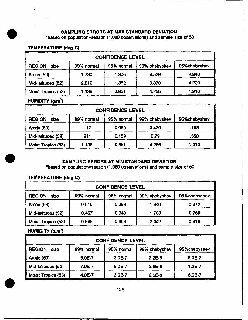
SAMPLING ERRORS AT MAX STANDARD DEVIATION

*based on population-season (1,080 observations) and sample size of 50

TEMPERATURE (deg C)

CONFIDENCE LEVEL

REGION size 99% normal 95% normal 99% chebyshev 95%chebyshev

Arctic (59) 1.730 1.306 6.529 2.940

Mid-latitudes (52) 2.510 1.882 9.370 4.220

Moist Tropics (53) 1.136 0.851 4.256 1.910

HUMIDITY (g/m3)

CONFIDENCE LEVEL

REGION size 99% normal 95% normal 99% chebyshev 95%chebyshev

Arctic (59) .117 0.088 0.439 .198

Mid-latitudes (52) .211 0.159 0.79 .350

Moist Tropics (53) 1.136 0.851 4.256 1.910

SAMPLING ERRORS AT MIN STANDARD DEVIATION*based on population-season (1,080 observations) and sample size of 50

TEMPERATURE (deg C)

CONFIDENCE LEVEL

REGION size 99% normal 95% normal 99% chebyshev 95%chebyshev

Arctic (59) 0.516 0.388 1.940 0.872

Mid-latitudes (52) 0.457 0.340 1.708 0.768

Moist Tropics (53) 0.545 0.408 2.042 0.919

HUMIDITY (g/m3)

CONFIDENCE LEVEL

REGION size 99% normal 95% normal 99% chebyshev 95%chebyshev

Arctic (59) 5.OE-7 3.0E-7 2.2E-6 9.0E-7

Mid-latitudes (52) 7.OE-7 5.OE-7 2.8E-6 1.2E-7

Moist Tropics (53) 4.OE-7 3.OE-7 2.OE-6 8.0E-7

C-5

SAMPLING ERRORS AT MAX STANDARD DEVIATION*based on large population ( > 500,000) with sample size of 50

TEMPERATURE (dog C)+

CONFIDENCE LEVEL

REGION size 99% normal 95% normal 99% chebyshev 95%chebyshev

Arctic (59) 1.780 1.342 6.710 3.020

Mid-latitudes (52) 2.570 1.930 9.614 4.330

Moist Tropics (53) 1.165 0.873 4.365 1.960

HUMIDITY (g/m3)

CONFIDENCE LEVEL

REGION size 99% normal 95% normal 99% chebyshev 95%chebyshev

Arctic (59) .120 0.090 0.451 .203

Mid-latitudes (52) .216 0.163 0.810 .364

Moist Tropics (53) 1.165 0.873 4.365 1.960

SAMPLING ERRORS AT MIN STANDARD DEVIATION

*based on large population( > 500,000) with sample size of 50

TEMPERATURE (dog C)

CONFIDENCE LEVEL

REGION size 99% ,",rmal 95% normal 99% chebyshev 95%chebyshev

Arctic (59) 0.5JO 0.398 1.993 0.897

Mid-latitudes (52) 0.469 0.352 1.752 0.788

Moist Tropics (53) )9 0.419 2.094 0.942

HUMIDITY (g/m2)

CONFIDENCE LEVEL

REGION size 994, normal 95% normal 99% chebyshev 95%chebyshev

Arctic (59) -E-7 4.OE-7 2.3E-6 1.OE-7

Mid-latitudes (52) 8.OE-7 1.3E-6 2.9E-6 7.OE-7

Moist Tropics (53) 5.0E-7 4.OE-7 2.1 E-6 9.OE-7

C-6

DISTRIBUTION

HQ AF/XOW, Pentagon, Washington, DC 20301 ....................................................... 1HQ USAF/XOOOW, Rm BD927, Washington, DC 2035054 ............................................. 1OSAF/SS, Rm 4C1062, Pentagon, Atto Weather, Washington, DC 203306560 ................................ 1USTC JSMJ4-OW, Scott Dr., Bldg 1900, Scott AFB, IL 62225-7001 .......................................... 1AWs/TrX/DOS/SCA, Losey St., Bldg 1521, Scott AFB, IL 62225-5008 ....................................... 1Dot 3, DOXW, PO Box 95004, Henderson, NV 89009-5004 ................................................ 1Det 4, AWS, Bldg 91027, Hurlburt Fld, FL 32544-5000 .................................................. 1OL1B, HQ AWS, Hanscom AFP , MA 01731-5000 ....................................................... 1eL-N, HQ AWS, ASL(SLCAS-BW-W), Bldg 1646, Rm 24, Missile Range, White Sands, NM 88002-5501 ............. 1HQ AFGWCVDOWSY, MEB39, 106 Peacekeeper Dr., Ste 2N3, Offutt AFP, NE 86113-4039 ...................... 1APSFC/DON, Stop 82, Bldg 715, Patrick Ave., Falcon AFB, CO 80912-5000 .................................. 1USAFETAC, Scott AFB, IL 62225-5000 .............................................................. 6OL-A, USAFETAC, Federal Building, Rm 305, Asheville, NC 28801-2723 .................................... 1AFSPACECOM/DOWA, Bldg 1, Stop 7, Peterson Rd., Peterson AFB, CO 80914-5001 ........................... 1721SPTS Weather, STE 2-210, 1 Norad Rd, Cheyenne Mtn, CO 80914-6113 .................................. 150 OSS/WE, Stop 82, Falcon AFB, CO 80912-5000 ..................................................... 145W5, Bldg 423, C. St., Patrick AFB, FL 32925-6537 ................................................... 1AFTAC/DOW, Patrick AFP , FL 32925-5000 ........................................................... 130WS, Coral Rd., Bldg 21150, Vandenberg AFP, CA 93437-5000 ........................................... 121OSS,/GSW, Hamilton Rd., Stop 22, Peterson AFB, CO 80914.5000 ....................................... 1SSD/MWA, PO Box 92966, Lom Angeles, CA 90009.2960 ................................................. ISSD/IMO, PO Box 92960, Los Angeles, CA 90009.2960 .................................................. 1SM-ALC/LH-AWS, McClellan AFB, CA 95652-5609 ..................................................... 1CSTC/WE, 1080 Lockheed Way, Box 007, Bldg 1001, Sunnyvale, CA 94089-1230 .............................. 1OD 4/DX, Onizuka AFB, CA 94088-3430 ............................................................. 1SSD OD 4, Onizuka AFB, CA 94088-3430 ............................................................ 1Det 3, Space Systems, Bldg 430, Stop 77, Buckley ANGB, CO 80011-9599 .................................... 1USAFA/DFP, Atto Capt Paul Bellaire, Colorado Springs, CO 80840-5701 .................................... 1S AFMC4(1YDW, Bldg 266, Post 108P Chidlaw Rd.,Wright-Patterson AFB, OH 45433-5000 ........................ 1FASTC/TAW, 4115 Hebble Creek Rd., Ste 33, Wright-Patterson AFP, OH 45433-5637 .......................... 1ASD/WE, Bldg 91, 3rd St, Wright-Patterson AFB, OH 45433-6503 ......................................... 1AFITMCIR, Wright-Patterson AFB, OH 45433-6583 ..................................................... 1WL/DOWA, Wright-Patterson AFP , OH 45433-6543 .................................................... 1WI/DOW, Wright Patterson AFB, OH 45433-6543 ..................................................... 12750ABW/WE, Bldg 206, Area C, Skeel Av., Wright Patterson AFB, OH 45433-6543 ............................ 1FASTCoTAW, Wright-Patterson AFB, OH 45433-6543 ................................................... 1P /WA E, Kirtland AFB, NM 87117-5000 .............................................................. 1HQ AFOTEC/WE, Kirtland AFB, NM 87117-7001 ...................................................... 1RIWE, Grifflas AFB, NY 13441-5700 ............................................................... 1RteDOVL, 26 Electronic Pkwy, Bldg 106, Griffiss AFB, NY 13441-4514 ...................................... I3250SS/OSW, Florida Ave., Stop 22, Bldg 149, Tyndall AFB, IL 32403-5048 .................................. 1AFESC/RDXT, Bldg 1120, Stop 21, Tyndall AFP, FL 32403-5000 .......................................... 1ESDYWE, Vandenberg Dr., Bldg 1624, Hanscom AFB, MA 01731-5000 ...................................... 1PtMI/ML, Research Library, Hanscom AFB, MA 01731-5000 ............................................. 13246TW/DOW, Bldg 60, Rm 60, Eglin AFB, FL 32542-5000 ............................................... 1AF rTV/WE, Edwards AFB, CA 93523-5000 ........................................................... 1510 OSS/WE, Bldg 1200, Rm 6, Wolfe Ave, Edwards AFB, CA 93523-5000 ................................... 16585 TG/WE, Range Rd, Bldg 1183, Holloman AFB, NM 88330-5000 ....................................... 1SSD/SDW, PO Box 92960, Bldg 117, El Segundo, Los Angeles AFB, CA 90009-2960 ............................ 1UJT5VWE, Hill AFB, UT 84056-5000 ............................................................... IUSAFA/CWOSW, Air Field Dr., Bldg 9206, USAF Academy, CO 80840-5000 .................................. 1AFTAC/WS, Patrick AFB, FL 32925-5000 ............................................................ 1ESMC/WE, Patrick AFB, FL 32925-5000 ............................................................ 1OL-A, AFCOS, Site R, Fort Ritchie, MD 21719-5010.................................................... 1USAFALCENT RA, Pope AFB, NC 28308-5000 ........................................................ 1CCSO/C L, Tinker AFB, OK 73145-6340 .............................................................. 1304 ARB &IOOR, Portland LAP, OR 97218-2797. ....................................................... 1AFOSWNLQ Bolling AFB, DC 20332.5000 ............................................................ 1TFWC/WE, Nellis AFB, NV 89191-5000 .............................................................. 1S AMC^XOWR, Bldg P40 N, Martin Ave, Scott AFB, IL 62225-5000 .......................................... 1

DIST-1

1SOW/OGSW, Attn Lt Kelly, 150 Bennett, Bldg 90730, Hurlburt FLD, FL 32544-500 ......................... 1HQ AFSOCDOW, Bldg 1, Hurlburt FLD, FL 32544"500 ................................................ 1ATCIDOTW, Bldg 399, Pm B27, D St., East, Randolph AFB, TX 78150-5000 .................................. 1PACAF/DOW, Bldg 1102, Hickam AFB, HI 96853-5000 .................................................. IUSSTRATCOM, J315, 901 SAC BLVD, STE BA3, Offutt AFB, NE 68113-5000 ................................ 1ACC/DOW, Bldg 21, 30 Elm St, Ste 215, Langley AFB, VA 23685-2093 ...................................... 11WG, Bldg 168, Hardee St., Ft McPherson, GA 30300-5000 ............................................... 1USAFE/DOW, Unit 3060, Box 15, APO AE 09094-5000 .................................................. 117AF/DOW, Unit 4065, APO AE 0913M5000 .......................................................... 1COMNAVOCEANCOM, Code N312, Stennis Space Ctr, MS 39529.5000 ..................................... 2NAVOCEANO (Rusty Russum), Bldg 8100, Rm 203D, Stennis Space Ctr, MS 39522-5001 ........................ 2NAVOCEANO, Code 9220 (Tony Ortolano), Stennis Space Ctr, MS 39529-5001 ................................ 1Maury Oceanographic Library, Naval Oceanography Office, Stennis Space Ctr, MS 39522-5001 ................... 1Naval Research Laboratory, Monterey, CA 93943-5006 ................................................. 1Naval Research Laboratory, Code 4323, Washington, DC 20375 ..................................... ... 1Naval Postgraduate School, Chmn, Dept of Meteorology, Code 63, Monterey, CA 93943-5000 ..................... 1Naval Air Warfare Center-Weapons Division, Geophysical Scieoces Branch, Code 3254, Attn Mr. Roger Helvey,Point Mugu, CA 93042-5001 .............................................................. ....... 1Armed Forces Medical Intelligence Center, Information Services DivisionBldg 1607, Ft Detrick, Frederick, MD 21702-5004 ...................................................... 1Chief, APG Met Team, Bldg 1134, Attn AMSTE-TC-AM CAB, Aberdeen Proving Ground, MD 21005-5001 ........... 1Atmospheric Science. Laboratory (SLCAS-AS-I -- 10-2c), White Sands Missile Range, NM 88002-5501 .............. 1TECOM Atmos Sci Div, AMSTE-TC-AA (MacBlam), White Sands Missile Range, NM 88002-5504 ................. 1White; ,_ds Met Team, AMSTE-TC-AM (WS), White Sands Missile Range, NM 88002-5501 ..................... 1USA TECOM, ATTN: AMSTE-TC-AM (RE) TECOM Met Team, Redstone Arsenal, AL 35898-8052 ................. 1Director, U.S.A.-CETEC, Attn GL-AE (Whitmarsh), Fort Belvoir, VA 22060-5546 .............................. 1Technical Library, Dugway Proving Ground, Dugway, UT 84022-5000 ...................................... 1OFCM, Attn. Col Dumont, Suite 900,6010 Executive Blvd, Rockville, MD 20852 .............................. 1HQ NATO Staff Meteorological Officer IMSOPS APO AR 09724 ........................................... 1NOAA/MASC Library MC5, 325 Broadway, Boulder, CO 80303-3328 ........................................ 2NOAA Library-EOC4W5C4, Attn: ACQ, 6009 Executive Blvd, Rockville, MD 20852 ............................ 1NOAA4NESDIS (Attn. Nancy Everson, S/RA22), World Weather Bldg, Rm 703, Washington, DC 2023S ............ 1NGDC, NOAA, Mail Code FWGC4, 325 Broadway, Boulder, CO 80333-3328 .................................. INWS W/OSD, Bldg SSM C-2 East-West Hwy, Silver Spring, MD 20910 ...................................... 1NIST Pubs Production, Rm A635, Admin Bldg, Gaithersburg, MD 20899 .................................... IWSO, H & HS Marine Station Wea, MCAS Tustin CA 92710-000 ......................................... 1DTIC-FDAC, Cameron Station, Alexandria, VA 22304-6145 .............................................. 2AU L•SE, Maxwell AFB, AL 36112-5564 ............................................................. IAWSTL, Scott AFB, IL 62225-5438 ................................................................. 35

DIST-2