80 Monetary Policy & the econoMy Q3/12 – addenduM

8.1 IntroductionThe use of the final survey weights described in chapter 7 is sufficient when estimating population parameters. To calculate the corresponding correct variances or standard errors of these estimators, however, replicate weights, which are described here, are necessary.

HFCS sampling involves a variety of features such as stratification or cluster-sampling. Ignoring these features in statistical analysis will bias the estimated variances of point estimators. For example, if stratification is ignored, the standard errors will be too large; and if clusters are ignored, the standard errors will be too small. Furthermore, if design weights are ignored, the sampling distributions of the statistics underrepresent the observations with a low selection probability and overrepresent those with a high selection probability (Kolenikov, 2010).

Unfortunately, a problem that occurs frequently when statistical analysis takes into account a complex survey design with all its features is that the mathematical functions of the variance estimators are unknown. Therefore, performing a statistical analysis requires methods developed especially for the purpose of variance estimation. There are two general categories of variance estimation methods: replicate weights methods (also called replication or resampling methods) and linearization.1

Until recently, the literature preferred linearization to replication, mostly because it is requires less computational power. However, an important disadvan-tage of linearization is that confidentiality provisions do not allow the inclusion of all information necessary for linearization. One way to avoid the problem that certain information is not available for reasons of privacy is to use replicate weights. Since replicate weights consist of many variables and their values are based on information not provided to the user of the data set – e.g. stratum and primary sampling unit (PSU) variables – it is virtually impossible for the data user to identify a given respondent (Stata Library, 2012).

Moreover, the linearization method cannot be used for estimating the variance of nonlinear statistics (medians, quartiles, etc.) as it requires computing deriva-tives of smooth functions; however, quantile functions, for instance, are discon-tinuous. Replicate weights, by contrast, are well suited for estimating the variance of such statistics (Heeringa et al., 2010).

Given the above-mentioned confidentiality constraints and because the HFCS data in particular facilitate the analysis of distributional parameters such as medians and quartiles, we decided that the variance estimation method to be employed for the HFCS should be based on the use of replicate weights. In the following section we describe how replicate weights are constructed for the HFCS in Austria.

8.2 Construction of Replicate Weights8.2.1 The Replication Method

The replication method aims at estimating the variance of an estimated population parameter. The idea behind it is to estimate, in a first step, population parameters for individual subsets (so-called replicates) of the sample observations. In a second

8 construction of replicate Weights for Variance estimation

1 For a comprehensive overview of variance estimation methods, see Levy and Lemeshow (2008) or Heeringa et al. (2010).

construction of replicate Weights for Variance estimation

Monetary Policy & the econoMy Q3/12 – addenduM 81

step, the variability of these estimated population parameters across all replicates is calculated, resulting in the desired variance of the overall estimated population parameter (Levy and Lemeshow, 2008).

Instead of saving a whole sample for each replicate, it is more practical to vary the final survey weights. For example, instead of removing a sample observation to construct a certain replicate, it can be given a weight of zero in the replicate. Then the weights of the other observations in the same stratum need to be increased to ensure that the totals are unbiased for each replicate r (Kolenikov, 2010). The replicate weights wi

(r) for r=1,…, R will be published together with the HFCS data set.

There are different methods to form such replicates. The three major replica-tion methods used in the survey literature are balanced repeated replication, jackknife and bootstrap replication. Although in most cases, the estimators of all replication methods converge to one another as the sample increases, simulation studies have shown that for quantile estimation bootstrap and balanced repeated replication are better suited than the jackknife (Kovar et al., 1988). Finally, as balanced repeated replication works only in designs with exactly two PSUs per stratum, which is not the case in the HFCS in Austria, we decided to use the (rescaling) bootstrap procedure proposed by Rao and Wu (1988) and extended by Rao et al. (1992). This procedure is also in line with the provisions of the ECB’s Household Finance and Consumption Network.

The bootstrap procedure forms replicates based on repeated with-replacement sampling of the PSUs within a stratum. The idea is to mimic the original sampling procedure in order to obtain approximations to the sampling distributions of the relevant statistics.

8.2.2 Sampling Error Calculation Model

To mimic the original sampling procedure, we build a sampling error calculation model which is a simplification of the actual complex sample design (chapter 6). Such models are used because, in many cases, the complex sample design intended for data collection poses analytical problems for variance estimation (Heeringa et al., 2010).

In the HFCS in Austria, one necessary simplification of the sampling error calculation model compared with the original sampling procedure is to collapse strata with one single PSU because the bootstrap procedure requires at least two PSUs per stratum. Due to the specific stratification of the HFCS sample design, single-PSU strata are quite common in the sample: In 81 strata out of a total of 170, only one PSU was drawn. For the sampling error calculation model, every single-PSU stratum is paired with the geographically nearest stratum to form a single pseudo-stratum. Although collapsing strata produces an upward bias in the estimated variance, this bias is kept as small as possible by collapsing geographi-cally close strata and thus keeping the PSUs within one pseudo stratum very homogeneous. In this context it must be pointed out that upward biases of standard errors lead to a loss in statistical power. In general, however, this is more accept-able than negative biases of standard errors, which lead to results that will too often qualify as statistically significant.

Table 17 shows how stratum size (number of PSUs drawn per stratum) changes when the HFCS sampling error calculation model is used instead of the original

construction of replicate Weights for Variance estimation

82 Monetary Policy & the econoMy Q3/12 – addenduM

HFCS sample design: When collapsing strata in the sampling error calculation model, their number decreases from 170 to 89, which means stratification is still very high. Moreover, the mean stratum size increases from 2.5 PSUs to 4.7 PSUs per stratum.

Another simplification performed in the HFCS sampling error calculation model in contrast to the original sam-ple design is to assume that sampling variance stems mostly from the first stage of sampling (i.e. the selection of PSUs, and not that of households within each PSU). Therefore, two-stage sampling is reduced to single-stage sampling where all gross sample households within a drawn PSUs are selected into the replicate sample.

The sampling error calculation model does not require any further simplifica-tions. In particular, the nonresponse and poststratification weight adjustments are implemented exactly as in the original weighting procedures (chapter 7), and a finite population correction2 is performed.

8.2.3 Construction of Replicate Weights

The algorithm used to construct the HFCS replicate weights comprises the following steps:• Step 1: Draw mh PSUs with replacement within each pseudo-stratum h.• Step 2: Adjust the final survey weights of the drawn observations to create a new

set of replicate weights. In particular, apply the same nonresponse and poststra-tification weight adjustments (sections 7.2.3 and 7.2.4) as for the design weights and perform a finite population correction.

• Step 3: Repeat steps 1 and 2 R times to obtain r = 1,…,R sets of replicate weights.In step 1, the number of PSUs mh drawn in each stratum of size nh is set to mh= nh –1. This is a common choice that ensures the efficiency of the bootstrap estimators without leading to violations of the natural parameter ranges (Kolenikov, 2010).

In step 2, the final survey weights must be adjusted because some PSUs may be duplicates and some may not have been drawn at all. As a consequence, each replicate will be biased with respect to the target population and therefore, to obtain the replicate weights, the design weights must be adjusted in the same way they were adjusted when constructing the final survey weights (chapter 7). In addition, a finite population correction is necessary because in the original HFCS sample design PSUs are sampled without replacement (footnote 2).

Finally, in step 3, the higher the number of replicates R, the more precise the standard error estimates. We choose R = 1,000, which lies in the upper bound of the usual recommendations found in the literature (Kolenikov, 2010).

table 17

Comparison of HFCS Design Strata and HFCS Pseudo Strata

design strata Pseudo strata

number of strata 170 89Mean size 2.5 4.7Median size 2 3Minimum size 1 2Maximum size 15 15

Source: HFCS Austria 2010, OeNB.

Note: Stratum size as measured by PSUs drawn per stratum.

2 The finite population correction accounts for the reduction in variance that occurs when sampling without replacement from a finite population. This type of sampling is used in the sample design for the HFCS in Austria.

construction of replicate Weights for Variance estimation

Monetary Policy & the econoMy Q3/12 – addenduM 83

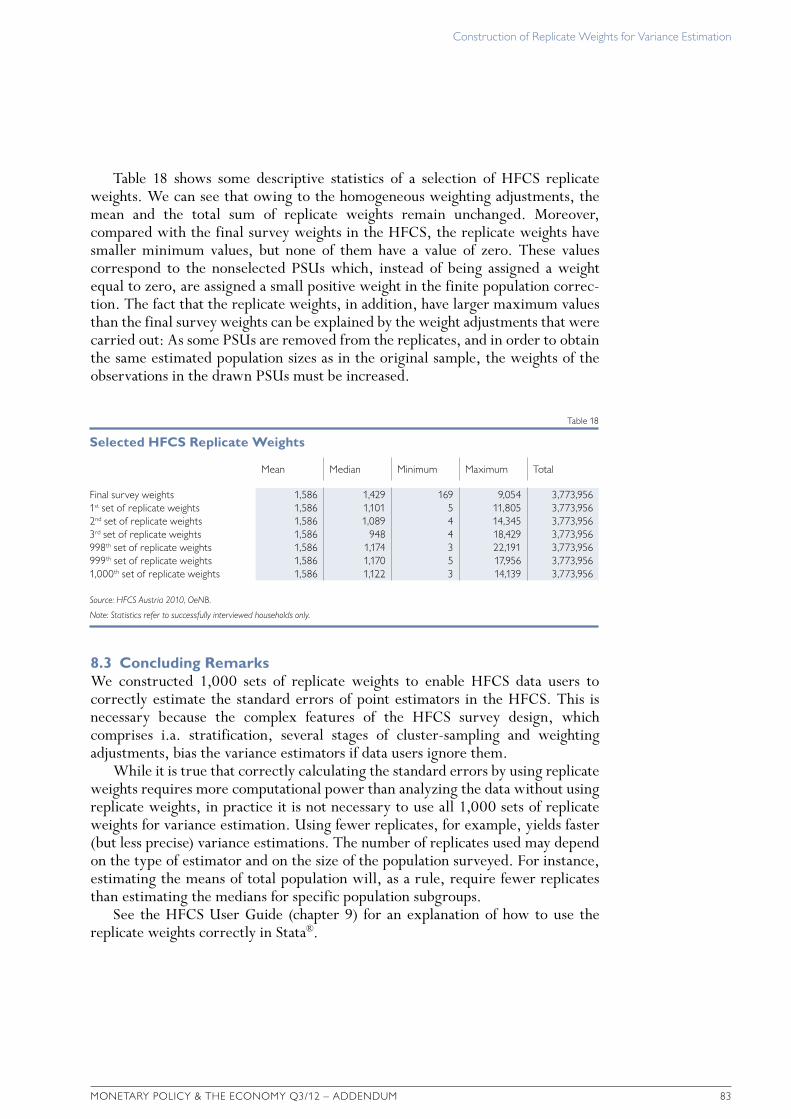
Table 18 shows some descriptive statistics of a selection of HFCS replicate weights. We can see that owing to the homogeneous weighting adjustments, the mean and the total sum of replicate weights remain unchanged. Moreover, compared with the final survey weights in the HFCS, the replicate weights have smaller minimum values, but none of them have a value of zero. These values correspond to the nonselected PSUs which, instead of being assigned a weight equal to zero, are assigned a small positive weight in the finite population correc-tion. The fact that the replicate weights, in addition, have larger maximum values than the final survey weights can be explained by the weight adjustments that were carried out: As some PSUs are removed from the replicates, and in order to obtain the same estimated population sizes as in the original sample, the weights of the observations in the drawn PSUs must be increased.

8.3 Concluding RemarksWe constructed 1,000 sets of replicate weights to enable HFCS data users to correctly estimate the standard errors of point estimators in the HFCS. This is necessary because the complex features of the HFCS survey design, which comprises i.a. stratification, several stages of cluster-sampling and weighting adjustments, bias the variance estimators if data users ignore them.

While it is true that correctly calculating the standard errors by using replicate weights requires more computational power than analyzing the data without using replicate weights, in practice it is not necessary to use all 1,000 sets of replicate weights for variance estimation. Using fewer replicates, for example, yields faster (but less precise) variance estimations. The number of replicates used may depend on the type of estimator and on the size of the population surveyed. For instance, estimating the means of total population will, as a rule, require fewer replicates than estimating the medians for specific population subgroups.

See the HFCS User Guide (chapter 9) for an explanation of how to use the replicate weights correctly in Stata®.

table 18

Selected HFCS Replicate Weights

Mean Median Minimum Maximum total

Final survey weights 1,586 1,429 169 9,054 3,773,9561st set of replicate weights 1,586 1,101 5 11,805 3,773,9562nd set of replicate weights 1,586 1,089 4 14,345 3,773,9563rd set of replicate weights 1,586 948 4 18,429 3,773,956998th set of replicate weights 1,586 1,174 3 22,191 3,773,956999th set of replicate weights 1,586 1,170 5 17,956 3,773,9561,000th set of replicate weights 1,586 1,122 3 14,139 3,773,956

Source: HFCS Austria 2010, OeNB.

Note: Statistics refer to successfully interviewed households only.