Embed Size (px)
Citation preview
Wearable Sensor System for Human Dynamics Analysis 117
Wearable Sensor System for Human Dynamics Analysis
Tao Liu, Yoshio Inoue, Kyoko Shibata and Rencheng Zheng
x
Wearable Sensor System for Human Dynamics Analysis
Tao Liu, Yoshio Inoue, Kyoko Shibata and Rencheng Zheng
Kochi University of Technology Japan
1. Introduction
In clinical applications the quantitative characterization of human kinematics and kinetics can be helpful for clinical doctors in monitoring patients’ recovery status; additionally, the quantitative results may help to strengthen confidence during their rehabilitation. The combination of 3D motion data obtained using an optical motion analysis system and ground reaction forces measured using a force plate has been successfully applied to perform human dynamics analysis (Stacoff et al., 2007; Yavuzer et al., 2008). However, the optical motion analysis method needs considerable workspace and high-speed graphic signal processing devices. Moreover, and if we use this analysis method in human kinetics analysis, the devices are expensive, while pre-calibration experiments and offline analysis of recorded pictures are especially complex and time-consuming. Therefore, these devices is limited to the laboratory research, and difficult to be used in daily life applications. Moreover, long-term, multi-step, and less restricted measurements in the study of gait evaluation are almost impossible when using the traditional methods, because a force plate can measure ground reaction force (GRF) during no more than a single stride, and the use of optical motion analysis is limited due to factors such as the limited mobility and line-of-sight of optical tracking equipment. Recently, many lower-cost and wearable sensor systems based to multi-sensor combinations including force sensitive resistors, inclinometers, goniometers, gyroscopes, and accelerometers have been proposed for triaxial joint angle measurement, joint moment and reaction force estimation, and muscle tension force calculation. As for researches of wearable GRF sensors, pressure sensors have been widely used to measure the distributed vertical component of GRF and analyze the loading pattern on soft tissue under the foot during gait (Faivre et al., 2004; Zhang et al., 2005), but in these systems the transverse component of GRF (friction forces) which is one of the main factors leading to fall were neglected. Some flexible force sensors designed using new materials such as silicon or polyimide and polydimethyl-siloxane have been proposed to measure the normal and transverse forces (Valdastri et al., 2005; Hwang et al., 2008), but force levels of these sensors using these expensive materials were limited to the measurements of small forces (about 50N). By mounting two common 6-axial force sensors beneath the front and rear boards of a special shoe, researchers have developed a instrumented shoe for ambulatory
8
www.intechopen.com
Mechatronic Systems, Applications118
measurements of CoP and triaxial GRF in successive walking trials (Veltink et al., 2005; Liedtke et al., 2007), and an application of the instrumented shoe to estimate moments and powers of the ankle was introduced by Schepers et al. (2007). About researches on body-mounted motion sensors, there are two major directions: one is about state recognition on daily physical activities including walking feature assessment (Sabatini et al., 2005; Aminian et al., 2002), walking condition classification (Coley et al., 2005; Najafi et al., 2002) and gait phase detection (Lau et al., 2008; Jasiewicz et al., 2006), in which the kinematic data obtained from inertial sensors (accelerometer or gyroscope) were directly used as inputs of the inference techniques; and another direction is for accurate measurement of human motion such as joint angles, body segment’s 3-D position and orientation, in which re-calibration and data processing by fusing different inertial sensors are important to decrease errors of the quantitative human motion analysis. In our research, a wearable sensor system which can measure human motion and ground reaction force will be developed and applied to estimate joint moment and muscle tension force, so we are focusing on the second direction for quantitative human motion analysis. There are growing interests in adopting commercial products of 3D motion sensor system, for example a smart sensor module MTx (Xsens, Netherlands) composed of a triaxial angular rate sensor, a triaxial accelerometer and a triaxial magnetic sensor, which can reconstruct triaxial angular displacements by means of a dedicated algorithm. However, it is sensitive to the effect of magnetic filed environment, and the dynamic accuracy of this sensor is about two degrees, which depends on type of experimental environments. In this chapter, a developed wearable sensor system including body-mounted motion sensors and a wearable force sensor is introduced for measuring lower limb orientations, 3D ground reaction forces, and estimating joint moments in human dynamics analysis. Moreover, a corresponding method of joint moment estimation using the wearable sensor system is proposed. This system will provide a lower-cost, more maneuverable, and more flexible sensing modality than those currently in use.
2. Wearable GRF Sensor
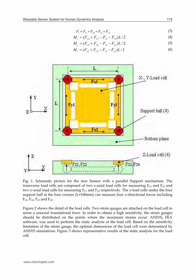
2.1 Mechanical Design and Dimension Optimization We developed a wearable multi-axial force sensor with a parallel mechanism to measure the ground reaction forces and moments in human dynamics analysis. First, the parallel mechanism for sensing triaxial forces and moments was introduced. As shown in Fig.1, the sensor is composed of a bottom plane, x-, y- and z-axial load cells, and four balls. When forces and moments are imposed to the bottom plane, they are transferred onto the four support balls. The support balls are connected with three load cells by point contacts. Therefore, only translational forces can be transferred to the corresponding load cells and measured using the strain gauges attached on the load cells. The x-axial load cell can measure FX1 and FX2. Similarly, the y-axial load cell measures FY1 and FY2, while the z-axial load cell measures FZ1, FZ2, FZ3 and FZ4. Based on these measured values, the three-axis forces and moments can be calculated by the use of the following equations:
21 xxx FFF (1)
21 yyy FFF (2)
3241 zzzzz FFFFF (3)
2/)( 4132 LFFFFM zzzzx (4)
2/)( 2143 LFFFFM zzzzy (5)
2/)( 1122 LFFFFM yxyxz (6)
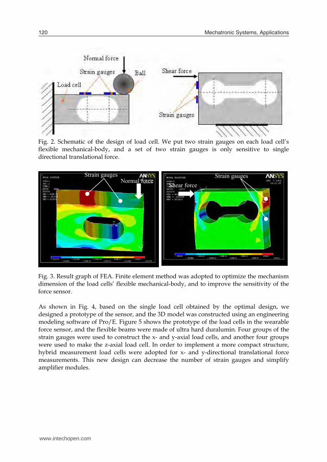
Fig. 1. Schematic picture for the new Sensor with a parallel Support mechanism. The transverse load cells are composed of two x-axial load cells for measuring Fx1 and Fx2 and two y-axial load cells for measuring Fy1 and Fy2 respectively. The z-load cells under the four support ball at the four corners (L=100mm) can measure four z-directional forces including Fz1, Fz2, Fz3 and Fz4. Figure 2 shows the detail of the load cells. Two strain gauges are attached on the load cell to sense a uniaxial translational force. In order to obtain a high sensitivity, the strain gauges should be distributed on the points where the maximum strains occur. ANSYS, FEA software, was used to perform the static analysis of the load cell. Based on the sensitivity limitation of the strain gauge, the optimal dimensions of the load cell were determined by ANSYS simulations. Figure 3 shows representative results of the static analysis for the load cell.
www.intechopen.com
Wearable Sensor System for Human Dynamics Analysis 119
measurements of CoP and triaxial GRF in successive walking trials (Veltink et al., 2005; Liedtke et al., 2007), and an application of the instrumented shoe to estimate moments and powers of the ankle was introduced by Schepers et al. (2007). About researches on body-mounted motion sensors, there are two major directions: one is about state recognition on daily physical activities including walking feature assessment (Sabatini et al., 2005; Aminian et al., 2002), walking condition classification (Coley et al., 2005; Najafi et al., 2002) and gait phase detection (Lau et al., 2008; Jasiewicz et al., 2006), in which the kinematic data obtained from inertial sensors (accelerometer or gyroscope) were directly used as inputs of the inference techniques; and another direction is for accurate measurement of human motion such as joint angles, body segment’s 3-D position and orientation, in which re-calibration and data processing by fusing different inertial sensors are important to decrease errors of the quantitative human motion analysis. In our research, a wearable sensor system which can measure human motion and ground reaction force will be developed and applied to estimate joint moment and muscle tension force, so we are focusing on the second direction for quantitative human motion analysis. There are growing interests in adopting commercial products of 3D motion sensor system, for example a smart sensor module MTx (Xsens, Netherlands) composed of a triaxial angular rate sensor, a triaxial accelerometer and a triaxial magnetic sensor, which can reconstruct triaxial angular displacements by means of a dedicated algorithm. However, it is sensitive to the effect of magnetic filed environment, and the dynamic accuracy of this sensor is about two degrees, which depends on type of experimental environments. In this chapter, a developed wearable sensor system including body-mounted motion sensors and a wearable force sensor is introduced for measuring lower limb orientations, 3D ground reaction forces, and estimating joint moments in human dynamics analysis. Moreover, a corresponding method of joint moment estimation using the wearable sensor system is proposed. This system will provide a lower-cost, more maneuverable, and more flexible sensing modality than those currently in use.
2. Wearable GRF Sensor
2.1 Mechanical Design and Dimension Optimization We developed a wearable multi-axial force sensor with a parallel mechanism to measure the ground reaction forces and moments in human dynamics analysis. First, the parallel mechanism for sensing triaxial forces and moments was introduced. As shown in Fig.1, the sensor is composed of a bottom plane, x-, y- and z-axial load cells, and four balls. When forces and moments are imposed to the bottom plane, they are transferred onto the four support balls. The support balls are connected with three load cells by point contacts. Therefore, only translational forces can be transferred to the corresponding load cells and measured using the strain gauges attached on the load cells. The x-axial load cell can measure FX1 and FX2. Similarly, the y-axial load cell measures FY1 and FY2, while the z-axial load cell measures FZ1, FZ2, FZ3 and FZ4. Based on these measured values, the three-axis forces and moments can be calculated by the use of the following equations:
21 xxx FFF (1)
21 yyy FFF (2)
3241 zzzzz FFFFF (3)
2/)( 4132 LFFFFM zzzzx (4)
2/)( 2143 LFFFFM zzzzy (5)
2/)( 1122 LFFFFM yxyxz (6)
Fig. 1. Schematic picture for the new Sensor with a parallel Support mechanism. The transverse load cells are composed of two x-axial load cells for measuring Fx1 and Fx2 and two y-axial load cells for measuring Fy1 and Fy2 respectively. The z-load cells under the four support ball at the four corners (L=100mm) can measure four z-directional forces including Fz1, Fz2, Fz3 and Fz4. Figure 2 shows the detail of the load cells. Two strain gauges are attached on the load cell to sense a uniaxial translational force. In order to obtain a high sensitivity, the strain gauges should be distributed on the points where the maximum strains occur. ANSYS, FEA software, was used to perform the static analysis of the load cell. Based on the sensitivity limitation of the strain gauge, the optimal dimensions of the load cell were determined by ANSYS simulations. Figure 3 shows representative results of the static analysis for the load cell.
www.intechopen.com
Mechatronic Systems, Applications120
Fig. 2. Schematic of the design of load cell. We put two strain gauges on each load cell’s flexible mechanical-body, and a set of two strain gauges is only sensitive to single directional translational force.
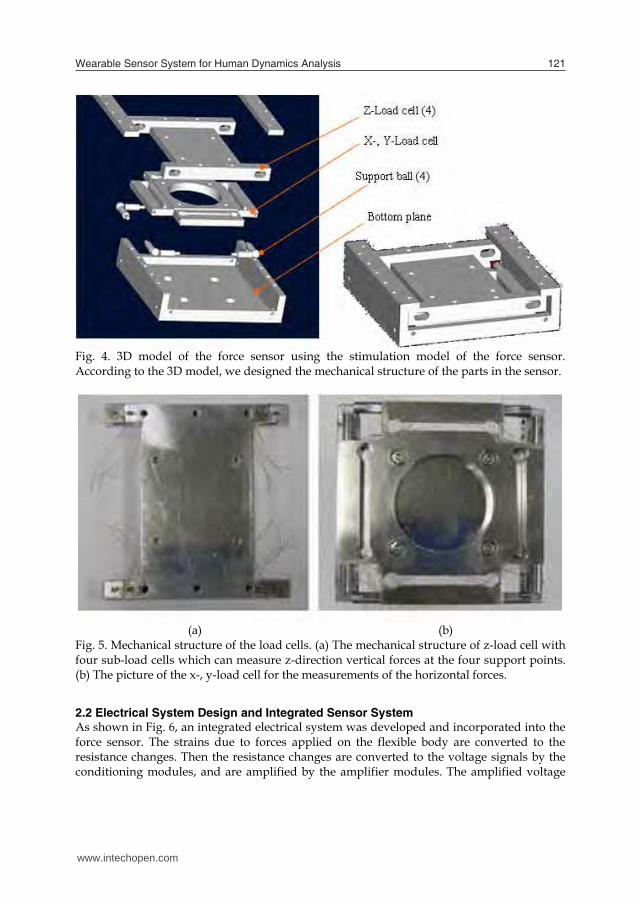
Fig. 3. Result graph of FEA. Finite element method was adopted to optimize the mechanism dimension of the load cells’ flexible mechanical-body, and to improve the sensitivity of the force sensor. As shown in Fig. 4, based on the single load cell obtained by the optimal design, we designed a prototype of the sensor, and the 3D model was constructed using an engineering modeling software of Pro/E. Figure 5 shows the prototype of the load cells in the wearable force sensor, and the flexible beams were made of ultra hard duralumin. Four groups of the strain gauges were used to construct the x- and y-axial load cells, and another four groups were used to make the z-axial load cell. In order to implement a more compact structure, hybrid measurement load cells were adopted for x- and y-directional translational force measurements. This new design can decrease the number of strain gauges and simplify amplifier modules.
Strain gauges Normal force
Shear force Strain gauges
Fig. 4. 3D model of the force sensor using the stimulation model of the force sensor. According to the 3D model, we designed the mechanical structure of the parts in the sensor.
(a) (b)
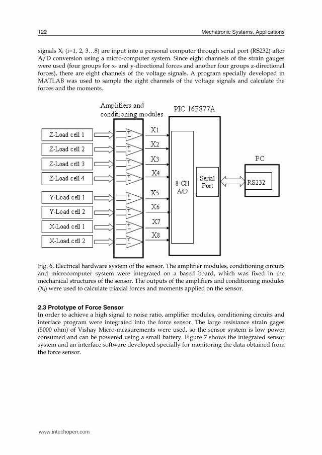
Fig. 5. Mechanical structure of the load cells. (a) The mechanical structure of z-load cell with four sub-load cells which can measure z-direction vertical forces at the four support points. (b) The picture of the x-, y-load cell for the measurements of the horizontal forces.
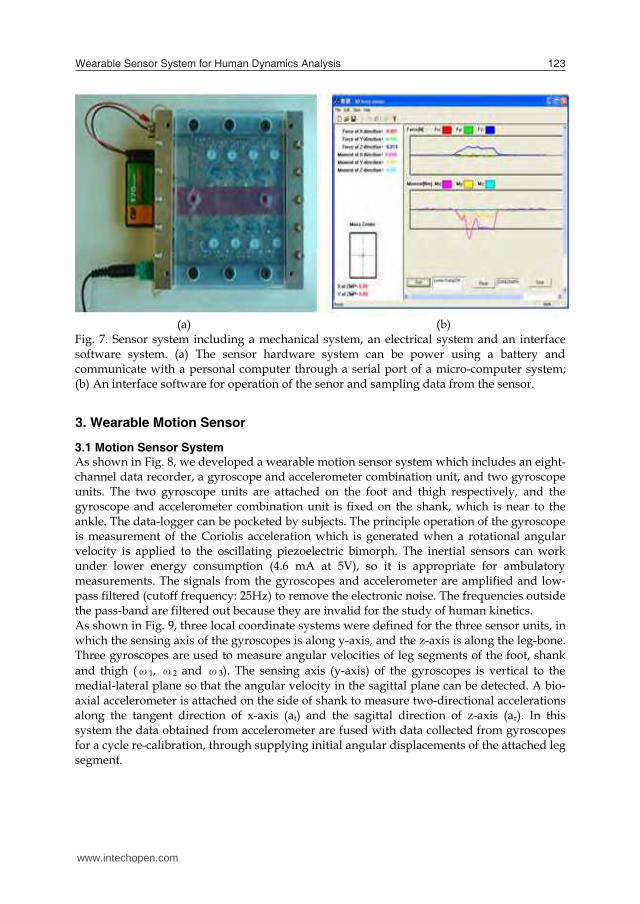
2.2 Electrical System Design and Integrated Sensor System As shown in Fig. 6, an integrated electrical system was developed and incorporated into the force sensor. The strains due to forces applied on the flexible body are converted to the resistance changes. Then the resistance changes are converted to the voltage signals by the conditioning modules, and are amplified by the amplifier modules. The amplified voltage
www.intechopen.com
Wearable Sensor System for Human Dynamics Analysis 121
Fig. 2. Schematic of the design of load cell. We put two strain gauges on each load cell’s flexible mechanical-body, and a set of two strain gauges is only sensitive to single directional translational force.
Fig. 3. Result graph of FEA. Finite element method was adopted to optimize the mechanism dimension of the load cells’ flexible mechanical-body, and to improve the sensitivity of the force sensor. As shown in Fig. 4, based on the single load cell obtained by the optimal design, we designed a prototype of the sensor, and the 3D model was constructed using an engineering modeling software of Pro/E. Figure 5 shows the prototype of the load cells in the wearable force sensor, and the flexible beams were made of ultra hard duralumin. Four groups of the strain gauges were used to construct the x- and y-axial load cells, and another four groups were used to make the z-axial load cell. In order to implement a more compact structure, hybrid measurement load cells were adopted for x- and y-directional translational force measurements. This new design can decrease the number of strain gauges and simplify amplifier modules.
Strain gauges Normal force
Shear force Strain gauges
Fig. 4. 3D model of the force sensor using the stimulation model of the force sensor. According to the 3D model, we designed the mechanical structure of the parts in the sensor.
(a) (b)
Fig. 5. Mechanical structure of the load cells. (a) The mechanical structure of z-load cell with four sub-load cells which can measure z-direction vertical forces at the four support points. (b) The picture of the x-, y-load cell for the measurements of the horizontal forces.
2.2 Electrical System Design and Integrated Sensor System As shown in Fig. 6, an integrated electrical system was developed and incorporated into the force sensor. The strains due to forces applied on the flexible body are converted to the resistance changes. Then the resistance changes are converted to the voltage signals by the conditioning modules, and are amplified by the amplifier modules. The amplified voltage
www.intechopen.com
Mechatronic Systems, Applications122
signals Xi (i=1, 2, 3…8) are input into a personal computer through serial port (RS232) after A/D conversion using a micro-computer system. Since eight channels of the strain gauges were used (four groups for x- and y-directional forces and another four groups z-directional forces), there are eight channels of the voltage signals. A program specially developed in MATLAB was used to sample the eight channels of the voltage signals and calculate the forces and the moments.
Fig. 6. Electrical hardware system of the sensor. The amplifier modules, conditioning circuits and microcomputer system were integrated on a based board, which was fixed in the mechanical structures of the sensor. The outputs of the amplifiers and conditioning modules (Xi) were used to calculate triaxial forces and moments applied on the sensor.
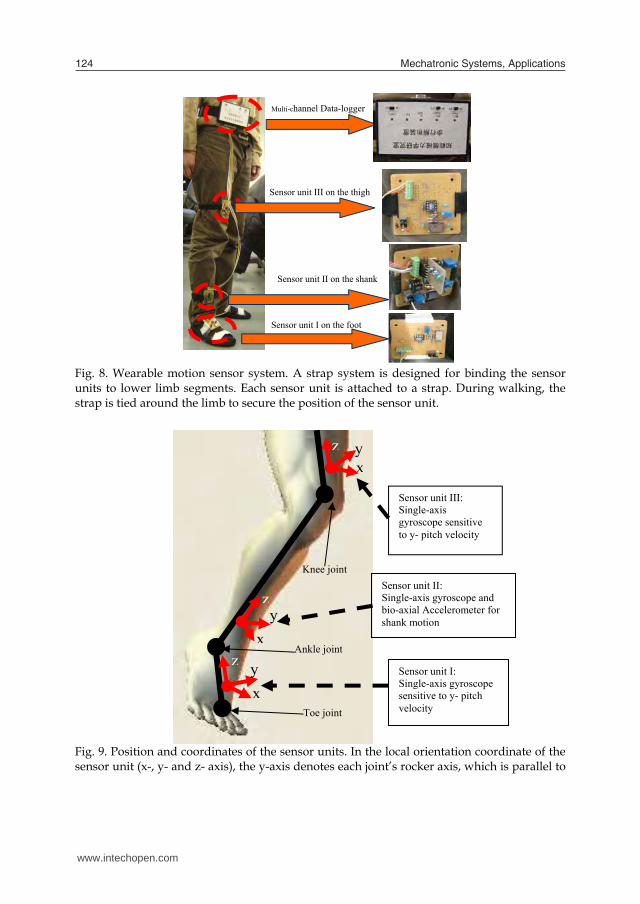
2.3 Prototype of Force Sensor In order to achieve a high signal to noise ratio, amplifier modules, conditioning circuits and interface program were integrated into the force sensor. The large resistance strain gages (5000 ohm) of Vishay Micro-measurements were used, so the sensor system is low power consumed and can be powered using a small battery. Figure 7 shows the integrated sensor system and an interface software developed specially for monitoring the data obtained from the force sensor.
(a) (b)
Fig. 7. Sensor system including a mechanical system, an electrical system and an interface software system. (a) The sensor hardware system can be power using a battery and communicate with a personal computer through a serial port of a micro-computer system; (b) An interface software for operation of the senor and sampling data from the sensor.
3. Wearable Motion Sensor
3.1 Motion Sensor System As shown in Fig. 8, we developed a wearable motion sensor system which includes an eight-channel data recorder, a gyroscope and accelerometer combination unit, and two gyroscope units. The two gyroscope units are attached on the foot and thigh respectively, and the gyroscope and accelerometer combination unit is fixed on the shank, which is near to the ankle. The data-logger can be pocketed by subjects. The principle operation of the gyroscope is measurement of the Coriolis acceleration which is generated when a rotational angular velocity is applied to the oscillating piezoelectric bimorph. The inertial sensors can work under lower energy consumption (4.6 mA at 5V), so it is appropriate for ambulatory measurements. The signals from the gyroscopes and accelerometer are amplified and low-pass filtered (cutoff frequency: 25Hz) to remove the electronic noise. The frequencies outside the pass-band are filtered out because they are invalid for the study of human kinetics. As shown in Fig. 9, three local coordinate systems were defined for the three sensor units, in which the sensing axis of the gyroscopes is along y-axis, and the z-axis is along the leg-bone. Three gyroscopes are used to measure angular velocities of leg segments of the foot, shank and thigh (ω1, ω2 and ω3). The sensing axis (y-axis) of the gyroscopes is vertical to the medial-lateral plane so that the angular velocity in the sagittal plane can be detected. A bio-axial accelerometer is attached on the side of shank to measure two-directional accelerations along the tangent direction of x-axis (at) and the sagittal direction of z-axis (ar). In this system the data obtained from accelerometer are fused with data collected from gyroscopes for a cycle re-calibration, through supplying initial angular displacements of the attached leg segment.
www.intechopen.com
Wearable Sensor System for Human Dynamics Analysis 123
signals Xi (i=1, 2, 3…8) are input into a personal computer through serial port (RS232) after A/D conversion using a micro-computer system. Since eight channels of the strain gauges were used (four groups for x- and y-directional forces and another four groups z-directional forces), there are eight channels of the voltage signals. A program specially developed in MATLAB was used to sample the eight channels of the voltage signals and calculate the forces and the moments.
Fig. 6. Electrical hardware system of the sensor. The amplifier modules, conditioning circuits and microcomputer system were integrated on a based board, which was fixed in the mechanical structures of the sensor. The outputs of the amplifiers and conditioning modules (Xi) were used to calculate triaxial forces and moments applied on the sensor.
2.3 Prototype of Force Sensor In order to achieve a high signal to noise ratio, amplifier modules, conditioning circuits and interface program were integrated into the force sensor. The large resistance strain gages (5000 ohm) of Vishay Micro-measurements were used, so the sensor system is low power consumed and can be powered using a small battery. Figure 7 shows the integrated sensor system and an interface software developed specially for monitoring the data obtained from the force sensor.
(a) (b)
Fig. 7. Sensor system including a mechanical system, an electrical system and an interface software system. (a) The sensor hardware system can be power using a battery and communicate with a personal computer through a serial port of a micro-computer system; (b) An interface software for operation of the senor and sampling data from the sensor.
3. Wearable Motion Sensor
3.1 Motion Sensor System As shown in Fig. 8, we developed a wearable motion sensor system which includes an eight-channel data recorder, a gyroscope and accelerometer combination unit, and two gyroscope units. The two gyroscope units are attached on the foot and thigh respectively, and the gyroscope and accelerometer combination unit is fixed on the shank, which is near to the ankle. The data-logger can be pocketed by subjects. The principle operation of the gyroscope is measurement of the Coriolis acceleration which is generated when a rotational angular velocity is applied to the oscillating piezoelectric bimorph. The inertial sensors can work under lower energy consumption (4.6 mA at 5V), so it is appropriate for ambulatory measurements. The signals from the gyroscopes and accelerometer are amplified and low-pass filtered (cutoff frequency: 25Hz) to remove the electronic noise. The frequencies outside the pass-band are filtered out because they are invalid for the study of human kinetics. As shown in Fig. 9, three local coordinate systems were defined for the three sensor units, in which the sensing axis of the gyroscopes is along y-axis, and the z-axis is along the leg-bone. Three gyroscopes are used to measure angular velocities of leg segments of the foot, shank and thigh (ω1, ω2 and ω3). The sensing axis (y-axis) of the gyroscopes is vertical to the medial-lateral plane so that the angular velocity in the sagittal plane can be detected. A bio-axial accelerometer is attached on the side of shank to measure two-directional accelerations along the tangent direction of x-axis (at) and the sagittal direction of z-axis (ar). In this system the data obtained from accelerometer are fused with data collected from gyroscopes for a cycle re-calibration, through supplying initial angular displacements of the attached leg segment.
www.intechopen.com
Mechatronic Systems, Applications124
Fig. 8. Wearable motion sensor system. A strap system is designed for binding the sensor units to lower limb segments. Each sensor unit is attached to a strap. During walking, the strap is tied around the limb to secure the position of the sensor unit.
Fig. 9. Position and coordinates of the sensor units. In the local orientation coordinate of the sensor unit (x-, y- and z- axis), the y-axis denotes each joint’s rocker axis, which is parallel to
xyzx
yz
x
Toe joint
Ankle joint
Knee joint
z y
Sensor unit I: Single-axis gyroscope sensitive to y- pitch velocity
Sensor unit II: Single-axis gyroscope and bio-axial Accelerometer for shank motion
Sensor unit III: Single-axisgyroscope sensitive to y- pitch velocity
Sensor unit II on the shank
Sensor unit III on the thigh
Sensor unit I on the foot
Multi-channel Data-loggerthe sensitive axis of the gyroscope, while x-axis and z-axis denote the unity vectors in the radial and tangential direction respectively.A multi-channel data-logger was also specially designed for the wearable motion sensor system. A micro-computer (PIC 16F877A) was used to develop the pocketed data-logger, and the sampled data from the inertial sensors could be saved in a SRAM which can keep recording for five minutes. An off-line motion analysis can be performed by feeding data saved in the SRAM to a personal computer through a RS232 communication module. Since gyroscope (ENC-03J), accelerometer-chip (ADXL202) and the PIC system are all devices with a lower energy consumption, the wearable sensor system could be powered using a battery of 300mAh (NiMH 30R7H).
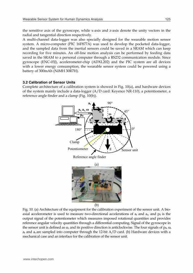
3.2 Calibration of Sensor Units Complete architecture of a calibration system is showed in Fig. 10(a), and hardware devices of the system mainly include a data-logger (A/D card: Keyence NR-110), a potentiometer, a reference angle finder and a clamp (Fig. 10(b)).
(a)
(b)
Fig. 10. (a) Architecture of the equipment for the calibration experiment of the sensor unit. A bio-axial accelerometer is used to measure two-directional accelerations of at and ar, and pθ is the output signal of the potentiometer which measures imposed rotational quantities and provides reference angular velocity quantities through a differential computing. Signal of the gyroscope in the sensor unit is defined as ω, and its positive direction is anticlockwise. The four signals of pθ, ω, at and ar are sampled into computer through the 12-bit A/D card. (b) Hardware devices with a mechanical case and an interface for the calibration of the sensor unit.
0°
90°
180°
gPotentiometer
Clamp
45°
at
ar
Reference angle finder
Sensor unit
ω at, ar, ω
pθ
www.intechopen.com
Wearable Sensor System for Human Dynamics Analysis 125
Fig. 8. Wearable motion sensor system. A strap system is designed for binding the sensor units to lower limb segments. Each sensor unit is attached to a strap. During walking, the strap is tied around the limb to secure the position of the sensor unit.
Fig. 9. Position and coordinates of the sensor units. In the local orientation coordinate of the sensor unit (x-, y- and z- axis), the y-axis denotes each joint’s rocker axis, which is parallel to
xyzx
yz
x
Toe joint
Ankle joint
Knee joint
z y
Sensor unit I: Single-axis gyroscope sensitive to y- pitch velocity
Sensor unit II: Single-axis gyroscope and bio-axial Accelerometer for shank motion
Sensor unit III: Single-axisgyroscope sensitive to y- pitch velocity
Sensor unit II on the shank
Sensor unit III on the thigh
Sensor unit I on the foot
Multi-channel Data-loggerthe sensitive axis of the gyroscope, while x-axis and z-axis denote the unity vectors in the radial and tangential direction respectively.A multi-channel data-logger was also specially designed for the wearable motion sensor system. A micro-computer (PIC 16F877A) was used to develop the pocketed data-logger, and the sampled data from the inertial sensors could be saved in a SRAM which can keep recording for five minutes. An off-line motion analysis can be performed by feeding data saved in the SRAM to a personal computer through a RS232 communication module. Since gyroscope (ENC-03J), accelerometer-chip (ADXL202) and the PIC system are all devices with a lower energy consumption, the wearable sensor system could be powered using a battery of 300mAh (NiMH 30R7H).
3.2 Calibration of Sensor Units Complete architecture of a calibration system is showed in Fig. 10(a), and hardware devices of the system mainly include a data-logger (A/D card: Keyence NR-110), a potentiometer, a reference angle finder and a clamp (Fig. 10(b)).
(a)
(b)
Fig. 10. (a) Architecture of the equipment for the calibration experiment of the sensor unit. A bio-axial accelerometer is used to measure two-directional accelerations of at and ar, and pθ is the output signal of the potentiometer which measures imposed rotational quantities and provides reference angular velocity quantities through a differential computing. Signal of the gyroscope in the sensor unit is defined as ω, and its positive direction is anticlockwise. The four signals of pθ, ω, at and ar are sampled into computer through the 12-bit A/D card. (b) Hardware devices with a mechanical case and an interface for the calibration of the sensor unit.
0°
90°
180°
gPotentiometer
Clamp
45°
at
ar
Reference angle finder
Sensor unit
ω at, ar, ω
pθ
www.intechopen.com
Mechatronic Systems, Applications126
The sensor units are calibrated in static state and dynamic state respectively. First, the calibration of the accelerometer sensor is carried out during the static state. The accelerometer in sensor unit is subjected to different gravity vectors by rotating a based axis that is connected with a potentiometer. Second, the dynamic calibration is completed to calibrate the gyroscopes and test the accelerometer in a dynamic condition. In both cases the calibration matrixes are computed using the least squares method. [Cθ] is calibration matrix for the angle position in (7). The matrix of the imposed quantities [θ] in a specific case can be recorded when the sensor unit is rotated to different positions on the angle finder plane; [pθ] is the matrix of the quantities acquired from the potentiometer, in the specific positions of a sensor unit. Angular displacement [θr] can be calculated using (8), and angular velocity of the sensor unit is obtained through the differential computing of the angular positions in a serial time. Gravity acceleration g projected to the two sensitive axes (at and ar) of the bio-axial accelerometer is estimated using (9) and (10). 1)( TT pppC (7) pCr (8)
)cos( rt gA (9)
)sin( rr gA (10)
[Cat] and [Car] are the calibration matrixes for the bio-axis accelerometer in (11) and (12), where [At] and [Ar] are the matrixes of the imposed quantities which were obtained when the sensor unit is subjected to different directional gravity vectors by rotating the sensor unit on the angle finder plane; [at] and [ar] are the matrixes of the quantities assessed by the accelerometer in the sensor unit. (13) and (14) give summations of the subjected gravity g and the segment motion acceleration on the two sensitive axes using the output signals of the bio-axial accelerometer. Table 1 shows the data of a sensor unit from a representative calibration experiment. 1)( T
ttT
ttat aaaAC (11)
1)( Trr
Trrar aaaAC (12) rarr
re aCA (13) tattre aCA (14)
[Cg] in (15) is the calibration matrix for gyroscope sensor in the sensor units, where [Vg] and [pθ] are the matrixes of the quantities respectively acquired from the gyroscope and potentiometer in a serial time (t); [Cθ] is the calibration matrix for the angle position in (7). Angular position [θr] can be calculated using (8), and angular velocity of the sensor unit is obtained through difference computing of the angular positions in the serial time. Gravity acceleration g projected to the two sensitive axes (at and ar) of the bio-axial accelerometer is estimated using (9) and (10).
1 T
gggg dtVdtVdtVpCC (15)
Angle finder θ (Degrees)
Potentiometer pθ (V)
Accelerometer at (V) ar (V)
0 1.438 2.541 3.004 -22.5 1.355 2.798 2.943 -45 1.284 2.985 2.813
-67.5 1.209 3.108 2.602 -90 1.134 3.138 2.369 22.5 1.512 2.294 2.969 45 1.595 2.096 2.849
67.5 1.671 1.937 2.663 90 1.748 1.882 2.457
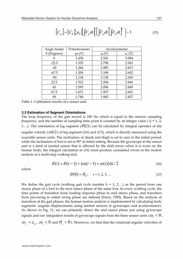
Table 1. Calibration results of a sensor unit.
3.3 Estimation of Segment Orientations The loop frequency of the gait record is 100 Hz which is equal to the sensors sampling frequency, and the number of sampling time point is counted by an integer value i (i = 1, 2, 3….). The orientation of leg segment ( )(i ) can be calculated by integral operator of the
angular velocity ( )(i ) of leg segment ((16) and (17)), which is directly measured using the wearable sensor units. The inclination of shank and thigh is set to zero in the initial period, while the inclination of foot is set to 90° at initial setting. Because the gyroscope in the sensor unit is a kind of inertial sensor that is affected by the drift errors when it is worn on the human body, the integral calculation in (16) must produce cumulated errors in the motion analysis of a multi-step walking trial.
2/))()1(()1()( tiiii (16) where
0)0( ; i = 1, 2, 3…. (17)
We define the gait cycle (walking gait cycle number k = 1, 2….) as the period from one stance phase of a foot to the next stance phase of the same foot. In every walking cycle, the time points of transition from loading response phase to mid stance phase, and transition from pre-swing to initial swing phase are defined (Parry, 1992). Based on the analysis of transition of the gait phases, the human motion analysis is implemented by calculating body segments’ angular displacements using inertial sensors of gyroscopes and accelerometers. As shown in Fig. 11, we can primarily detect the mid stance phase just using gyroscope signals and raw integration results of gyroscope signals from the three sensor units ( 0t ,
f , 0s and 0s ). Moreover, we find that the rotational angular velocities of
www.intechopen.com
Wearable Sensor System for Human Dynamics Analysis 127
The sensor units are calibrated in static state and dynamic state respectively. First, the calibration of the accelerometer sensor is carried out during the static state. The accelerometer in sensor unit is subjected to different gravity vectors by rotating a based axis that is connected with a potentiometer. Second, the dynamic calibration is completed to calibrate the gyroscopes and test the accelerometer in a dynamic condition. In both cases the calibration matrixes are computed using the least squares method. [Cθ] is calibration matrix for the angle position in (7). The matrix of the imposed quantities [θ] in a specific case can be recorded when the sensor unit is rotated to different positions on the angle finder plane; [pθ] is the matrix of the quantities acquired from the potentiometer, in the specific positions of a sensor unit. Angular displacement [θr] can be calculated using (8), and angular velocity of the sensor unit is obtained through the differential computing of the angular positions in a serial time. Gravity acceleration g projected to the two sensitive axes (at and ar) of the bio-axial accelerometer is estimated using (9) and (10). 1)( TT pppC (7) pCr (8)
)cos( rt gA (9)
)sin( rr gA (10)
[Cat] and [Car] are the calibration matrixes for the bio-axis accelerometer in (11) and (12), where [At] and [Ar] are the matrixes of the imposed quantities which were obtained when the sensor unit is subjected to different directional gravity vectors by rotating the sensor unit on the angle finder plane; [at] and [ar] are the matrixes of the quantities assessed by the accelerometer in the sensor unit. (13) and (14) give summations of the subjected gravity g and the segment motion acceleration on the two sensitive axes using the output signals of the bio-axial accelerometer. Table 1 shows the data of a sensor unit from a representative calibration experiment. 1)( T
ttT
ttat aaaAC (11)
1)( Trr
Trrar aaaAC (12) rarr
re aCA (13) tattre aCA (14)
[Cg] in (15) is the calibration matrix for gyroscope sensor in the sensor units, where [Vg] and [pθ] are the matrixes of the quantities respectively acquired from the gyroscope and potentiometer in a serial time (t); [Cθ] is the calibration matrix for the angle position in (7). Angular position [θr] can be calculated using (8), and angular velocity of the sensor unit is obtained through difference computing of the angular positions in the serial time. Gravity acceleration g projected to the two sensitive axes (at and ar) of the bio-axial accelerometer is estimated using (9) and (10).
1 T
gggg dtVdtVdtVpCC (15)
Angle finder θ (Degrees)
Potentiometer pθ (V)
Accelerometer at (V) ar (V)
0 1.438 2.541 3.004 -22.5 1.355 2.798 2.943 -45 1.284 2.985 2.813
-67.5 1.209 3.108 2.602 -90 1.134 3.138 2.369 22.5 1.512 2.294 2.969 45 1.595 2.096 2.849
67.5 1.671 1.937 2.663 90 1.748 1.882 2.457
Table 1. Calibration results of a sensor unit.
3.3 Estimation of Segment Orientations The loop frequency of the gait record is 100 Hz which is equal to the sensors sampling frequency, and the number of sampling time point is counted by an integer value i (i = 1, 2, 3….). The orientation of leg segment ( )(i ) can be calculated by integral operator of the
angular velocity ( )(i ) of leg segment ((16) and (17)), which is directly measured using the wearable sensor units. The inclination of shank and thigh is set to zero in the initial period, while the inclination of foot is set to 90° at initial setting. Because the gyroscope in the sensor unit is a kind of inertial sensor that is affected by the drift errors when it is worn on the human body, the integral calculation in (16) must produce cumulated errors in the motion analysis of a multi-step walking trial.
2/))()1(()1()( tiiii (16) where
0)0( ; i = 1, 2, 3…. (17)
We define the gait cycle (walking gait cycle number k = 1, 2….) as the period from one stance phase of a foot to the next stance phase of the same foot. In every walking cycle, the time points of transition from loading response phase to mid stance phase, and transition from pre-swing to initial swing phase are defined (Parry, 1992). Based on the analysis of transition of the gait phases, the human motion analysis is implemented by calculating body segments’ angular displacements using inertial sensors of gyroscopes and accelerometers. As shown in Fig. 11, we can primarily detect the mid stance phase just using gyroscope signals and raw integration results of gyroscope signals from the three sensor units ( 0t ,
f , 0s and 0s ). Moreover, we find that the rotational angular velocities of
www.intechopen.com
Mechatronic Systems, Applications128
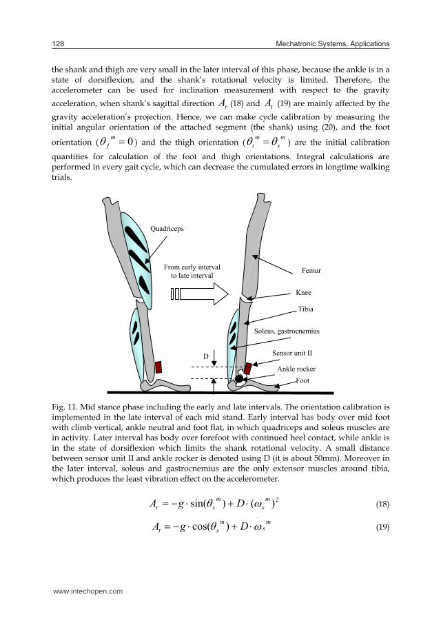
the shank and thigh are very small in the later interval of this phase, because the ankle is in a state of dorsiflexion, and the shank’s rotational velocity is limited. Therefore, the accelerometer can be used for inclination measurement with respect to the gravity acceleration, when shank’s sagittal direction rA (18) and tA (19) are mainly affected by the gravity acceleration’s projection. Hence, we can make cycle calibration by measuring the initial angular orientation of the attached segment (the shank) using (20), and the foot
orientation ( 0mf ) and the thigh orientation (
ms
mt ) are the initial calibration
quantities for calculation of the foot and thigh orientations. Integral calculations are performed in every gait cycle, which can decrease the cumulated errors in longtime walking trials.
Fig. 11. Mid stance phase including the early and late intervals. The orientation calibration is implemented in the late interval of each mid stand. Early interval has body over mid foot with climb vertical, ankle neutral and foot flat, in which quadriceps and soleus muscles are in activity. Later interval has body over forefoot with continued heel contact, while ankle is in the state of dorsiflexion which limits the shank rotational velocity. A small distance between sensor unit II and ankle rocker is denoted using D (it is about 50mm). Moreover in the later interval, soleus and gastrocnemius are the only extensor muscles around tibia, which produces the least vibration effect on the accelerometer.
2)()sin( ms
msr DgA (18)
ms
mst DgA
)cos( (19)
Tibia
Femur
Soleus, gastrocnemius
FootAnkle rocker
Sensor unit II
Knee
D
Quadriceps
From early interval to late interval
)/arctan( trms AA (20)
However, the heel of some subjects (e.g. paralytic patient) may never contact the ground, and in this case the proposed direct inference algorithm can not be used for the cycle recalibration to decrease the integration errors. A linear regression method was developed to calculate drift errors coming from the digital integration, in which we supposed the error increase in a linear function. We let i be the direct integration results by (16), and m be reference static inclination angle measured using accelerometer by (20). The summary error ( mie ) is obtained from a single walking trial during which subjects are required to
walk along a straight leading line. Error estimation function ( )(ie ) is given as following equation based to a linear regression.
titi mie /)()( , i = 1, 2, 3….t (21)
)()()( iii ec (22)
where t is the sampling time and )(ic was defined as the estimated angle after an error correction.
4. Calculation of Joint Moment
Based on the measurements of GRF and segment orientations using the two sensor systems, we can calculate lower limb’s joint moments which are useful for evaluating in vivo forces of human body during gait. For calculation purposes, such as estimating joint moments of the ankle during loading response and terminal stance phases (Parry, 1992), all vectors including joint displacement vector, GRF vector and gravity vector have to be expressed in the same coordinate system, being the global coordinate system. The y-axis of the global coordinate system was chosen to represent the anterior-posterior direction of human movement, and the z-axis was made vertical, while the x-axis was chosen such that the resulting global coordinate system would be right-handed. The origin of the global coordinate system was fixed to a point around the anatomical center of the ankle when the wearable force sensor was worn under the foot. The GRF and the moments measured using the wearable force sensor are expressed by the vectors in (23), and the coordinates of center of pressure (CoP)
CoPgx in the global frame is calculated using the following equation:
zg
yg
xg
GRFg
FFF
F
zg
yg
xg
GRFg
MMM
M
0z
gy
gz
gy
g
CoPg
FMFM
x
(23)
www.intechopen.com
Wearable Sensor System for Human Dynamics Analysis 129
the shank and thigh are very small in the later interval of this phase, because the ankle is in a state of dorsiflexion, and the shank’s rotational velocity is limited. Therefore, the accelerometer can be used for inclination measurement with respect to the gravity acceleration, when shank’s sagittal direction rA (18) and tA (19) are mainly affected by the gravity acceleration’s projection. Hence, we can make cycle calibration by measuring the initial angular orientation of the attached segment (the shank) using (20), and the foot
orientation ( 0mf ) and the thigh orientation (
ms
mt ) are the initial calibration
quantities for calculation of the foot and thigh orientations. Integral calculations are performed in every gait cycle, which can decrease the cumulated errors in longtime walking trials.
Fig. 11. Mid stance phase including the early and late intervals. The orientation calibration is implemented in the late interval of each mid stand. Early interval has body over mid foot with climb vertical, ankle neutral and foot flat, in which quadriceps and soleus muscles are in activity. Later interval has body over forefoot with continued heel contact, while ankle is in the state of dorsiflexion which limits the shank rotational velocity. A small distance between sensor unit II and ankle rocker is denoted using D (it is about 50mm). Moreover in the later interval, soleus and gastrocnemius are the only extensor muscles around tibia, which produces the least vibration effect on the accelerometer.
2)()sin( ms
msr DgA (18)
ms
mst DgA
)cos( (19)
Tibia
Femur
Soleus, gastrocnemius
FootAnkle rocker
Sensor unit II
Knee
D
Quadriceps
From early interval to late interval
)/arctan( trms AA (20)
However, the heel of some subjects (e.g. paralytic patient) may never contact the ground, and in this case the proposed direct inference algorithm can not be used for the cycle recalibration to decrease the integration errors. A linear regression method was developed to calculate drift errors coming from the digital integration, in which we supposed the error increase in a linear function. We let i be the direct integration results by (16), and m be reference static inclination angle measured using accelerometer by (20). The summary error ( mie ) is obtained from a single walking trial during which subjects are required to
walk along a straight leading line. Error estimation function ( )(ie ) is given as following equation based to a linear regression.
titi mie /)()( , i = 1, 2, 3….t (21)
)()()( iii ec (22)
where t is the sampling time and )(ic was defined as the estimated angle after an error correction.
4. Calculation of Joint Moment
Based on the measurements of GRF and segment orientations using the two sensor systems, we can calculate lower limb’s joint moments which are useful for evaluating in vivo forces of human body during gait. For calculation purposes, such as estimating joint moments of the ankle during loading response and terminal stance phases (Parry, 1992), all vectors including joint displacement vector, GRF vector and gravity vector have to be expressed in the same coordinate system, being the global coordinate system. The y-axis of the global coordinate system was chosen to represent the anterior-posterior direction of human movement, and the z-axis was made vertical, while the x-axis was chosen such that the resulting global coordinate system would be right-handed. The origin of the global coordinate system was fixed to a point around the anatomical center of the ankle when the wearable force sensor was worn under the foot. The GRF and the moments measured using the wearable force sensor are expressed by the vectors in (23), and the coordinates of center of pressure (CoP)
CoPgx in the global frame is calculated using the following equation:
zg
yg
xg
GRFg
FFF
F
zg
yg
xg
GRFg
MMM
M
0z
gy
gz
gy
g
CoPg
FMFM
x
(23)
www.intechopen.com
Mechatronic Systems, Applications130
The ankle, knee and hip joint moments in the global coordinates system can be calculated using the inverse dynamic method (Hof, 1992; Zheng et al., 2008)
k
iii
k
iiikk
gi
g
k
iikk
gi
gGRFkk
gCoP
gkk
g
Idtdamrr
gmrrFrrM
111,
11,1,1, )(
, k=1, 2, 3, (24)
where
2,1Mg ,
3,2Mg and
4,3Mg represent the ankle, knee and hip joint moments respectively.
CoPgr is referred as the position vector pointing from the origin of the global coordinate
system to the CoP. 1r
g ,2r
g and 3r
g are the position vectors from the origin of the global coordinates system to the centers of the ankle, knee and hip joints.
2,1rg ,
3,2rg and
4,3rg are the
position vectors from the origin of the global coordinates system to the center of mass (CoM) of the foot, shank and thigh respectively. The mass of the foot, shank and thigh was defined as 1m , 2m and
3m respectively. 1a , 2a and 3a are the accelerations of the CoM of the foot,
shank and thigh respectively. 1I , 2I and 3I are the inertia moments of the foot, shank and
thigh respectively. The angular velocities of the foot, shank and thigh were obtained by the
differential operators ( 1
, 2
and 3
).
5. Experiment Study
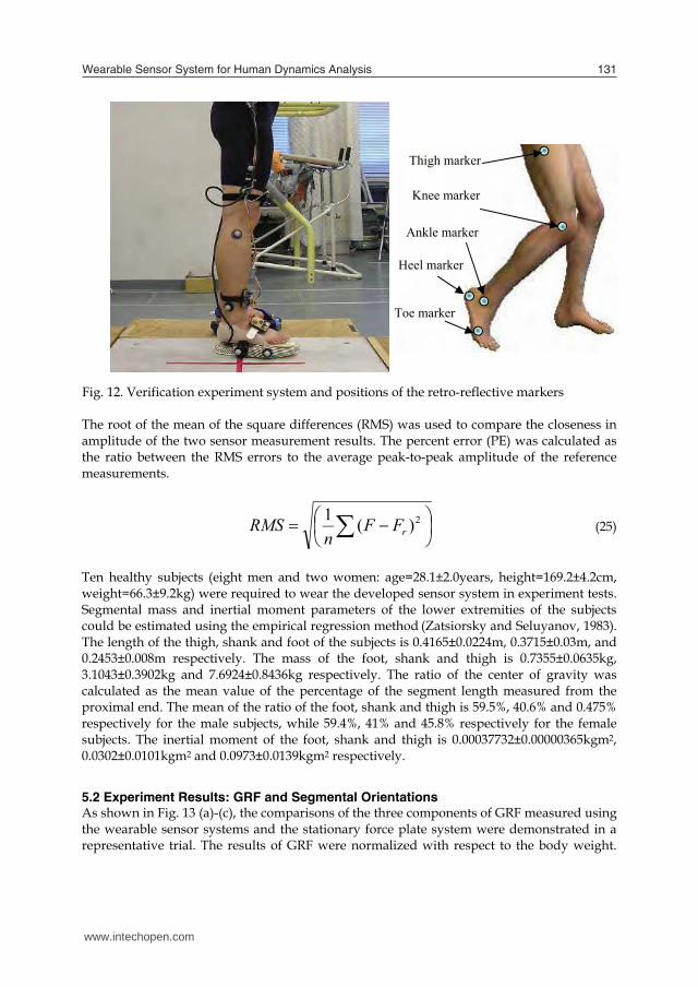
5.1 Experiment Method To validate the sensor system performance we have compared the quantitative results of the sensor system with the measurements obtained with a commercial optical motion analysis system Hi-DCam (NAC image technology. Japan). The commercial motion analysis system can track and measure three-dimensional (3-D) trajectories of retro-reflective markers placed on the subject’s body, as shown in Fig. 12. The cameras with a sampling frequency of 100 Hz were used to track the marker positions with an accuracy of about 1 mm. A stationary force plate of EFP-S-2KNSA12 (Kyowa co. Japan) was also used as a reference sensor to validate the measurement of the developed force sensor. In our experiment, these sensor systems simultaneously worked in the measurements of human force and motion. The data from the reference sensor systems and our developed sensor systems were sampled at the same time, and were compared.
Fig. 12. Verification experiment system and positions of the retro-reflective markers The root of the mean of the square differences (RMS) was used to compare the closeness in amplitude of the two sensor measurement results. The percent error (PE) was calculated as the ratio between the RMS errors to the average peak-to-peak amplitude of the reference measurements.
2)(1rFF
nRMS (25)
Ten healthy subjects (eight men and two women: age=28.1±2.0years, height=169.2±4.2cm, weight=66.3±9.2kg) were required to wear the developed sensor system in experiment tests. Segmental mass and inertial moment parameters of the lower extremities of the subjects could be estimated using the empirical regression method (Zatsiorsky and Seluyanov, 1983). The length of the thigh, shank and foot of the subjects is 0.4165±0.0224m, 0.3715±0.03m, and 0.2453±0.008m respectively. The mass of the foot, shank and thigh is 0.7355±0.0635kg, 3.1043±0.3902kg and 7.6924±0.8436kg respectively. The ratio of the center of gravity was calculated as the mean value of the percentage of the segment length measured from the proximal end. The mean of the ratio of the foot, shank and thigh is 59.5%, 40.6% and 0.475% respectively for the male subjects, while 59.4%, 41% and 45.8% respectively for the female subjects. The inertial moment of the foot, shank and thigh is 0.00037732±0.00000365kgm2, 0.0302±0.0101kgm2 and 0.0973±0.0139kgm2 respectively.
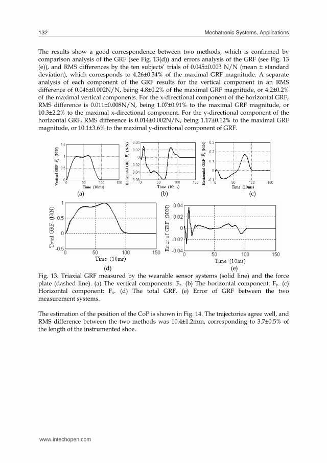
5.2 Experiment Results: GRF and Segmental Orientations As shown in Fig. 13 (a)-(c), the comparisons of the three components of GRF measured using the wearable sensor systems and the stationary force plate system were demonstrated in a representative trial. The results of GRF were normalized with respect to the body weight.
Toe marker
Heel marker
Ankle marker
Knee marker
Thigh marker
www.intechopen.com
Wearable Sensor System for Human Dynamics Analysis 131
The ankle, knee and hip joint moments in the global coordinates system can be calculated using the inverse dynamic method (Hof, 1992; Zheng et al., 2008)
k
iii
k
iiikk
gi
g
k
iikk
gi
gGRFkk
gCoP
gkk
g
Idtdamrr
gmrrFrrM
111,
11,1,1, )(
, k=1, 2, 3, (24)
where
2,1Mg ,
3,2Mg and
4,3Mg represent the ankle, knee and hip joint moments respectively.
CoPgr is referred as the position vector pointing from the origin of the global coordinate
system to the CoP. 1r
g ,2r
g and 3r
g are the position vectors from the origin of the global coordinates system to the centers of the ankle, knee and hip joints.
2,1rg ,
3,2rg and
4,3rg are the
position vectors from the origin of the global coordinates system to the center of mass (CoM) of the foot, shank and thigh respectively. The mass of the foot, shank and thigh was defined as 1m , 2m and
3m respectively. 1a , 2a and 3a are the accelerations of the CoM of the foot,
shank and thigh respectively. 1I , 2I and 3I are the inertia moments of the foot, shank and
thigh respectively. The angular velocities of the foot, shank and thigh were obtained by the
differential operators ( 1
, 2
and 3
).
5. Experiment Study
5.1 Experiment Method To validate the sensor system performance we have compared the quantitative results of the sensor system with the measurements obtained with a commercial optical motion analysis system Hi-DCam (NAC image technology. Japan). The commercial motion analysis system can track and measure three-dimensional (3-D) trajectories of retro-reflective markers placed on the subject’s body, as shown in Fig. 12. The cameras with a sampling frequency of 100 Hz were used to track the marker positions with an accuracy of about 1 mm. A stationary force plate of EFP-S-2KNSA12 (Kyowa co. Japan) was also used as a reference sensor to validate the measurement of the developed force sensor. In our experiment, these sensor systems simultaneously worked in the measurements of human force and motion. The data from the reference sensor systems and our developed sensor systems were sampled at the same time, and were compared.
Fig. 12. Verification experiment system and positions of the retro-reflective markers The root of the mean of the square differences (RMS) was used to compare the closeness in amplitude of the two sensor measurement results. The percent error (PE) was calculated as the ratio between the RMS errors to the average peak-to-peak amplitude of the reference measurements.
2)(1rFF
nRMS (25)
Ten healthy subjects (eight men and two women: age=28.1±2.0years, height=169.2±4.2cm, weight=66.3±9.2kg) were required to wear the developed sensor system in experiment tests. Segmental mass and inertial moment parameters of the lower extremities of the subjects could be estimated using the empirical regression method (Zatsiorsky and Seluyanov, 1983). The length of the thigh, shank and foot of the subjects is 0.4165±0.0224m, 0.3715±0.03m, and 0.2453±0.008m respectively. The mass of the foot, shank and thigh is 0.7355±0.0635kg, 3.1043±0.3902kg and 7.6924±0.8436kg respectively. The ratio of the center of gravity was calculated as the mean value of the percentage of the segment length measured from the proximal end. The mean of the ratio of the foot, shank and thigh is 59.5%, 40.6% and 0.475% respectively for the male subjects, while 59.4%, 41% and 45.8% respectively for the female subjects. The inertial moment of the foot, shank and thigh is 0.00037732±0.00000365kgm2, 0.0302±0.0101kgm2 and 0.0973±0.0139kgm2 respectively.
5.2 Experiment Results: GRF and Segmental Orientations As shown in Fig. 13 (a)-(c), the comparisons of the three components of GRF measured using the wearable sensor systems and the stationary force plate system were demonstrated in a representative trial. The results of GRF were normalized with respect to the body weight.
Toe marker
Heel marker
Ankle marker
Knee marker
Thigh marker
www.intechopen.com
Mechatronic Systems, Applications132
The results show a good correspondence between two methods, which is confirmed by comparison analysis of the GRF (see Fig. 13(d)) and errors analysis of the GRF (see Fig. 13 (e)), and RMS differences by the ten subjects’ trials of 0.045±0.003 N/N (mean ± standard deviation), which corresponds to 4.26±0.34% of the maximal GRF magnitude. A separate analysis of each component of the GRF results for the vertical component in an RMS difference of 0.046±0.002N/N, being 4.8±0.2% of the maximal GRF magnitude, or 4.2±0.2% of the maximal vertical components. For the x-directional component of the horizontal GRF, RMS difference is 0.011±0.008N/N, being 1.07±0.91% to the maximal GRF magnitude, or 10.3±2.2% to the maximal x-directional component. For the y-directional component of the horizontal GRF, RMS difference is 0.014±0.002N/N, being 1.17±0.12% to the maximal GRF magnitude, or 10.1±3.6% to the maximal y-directional component of GRF.
(a) (b) (c)
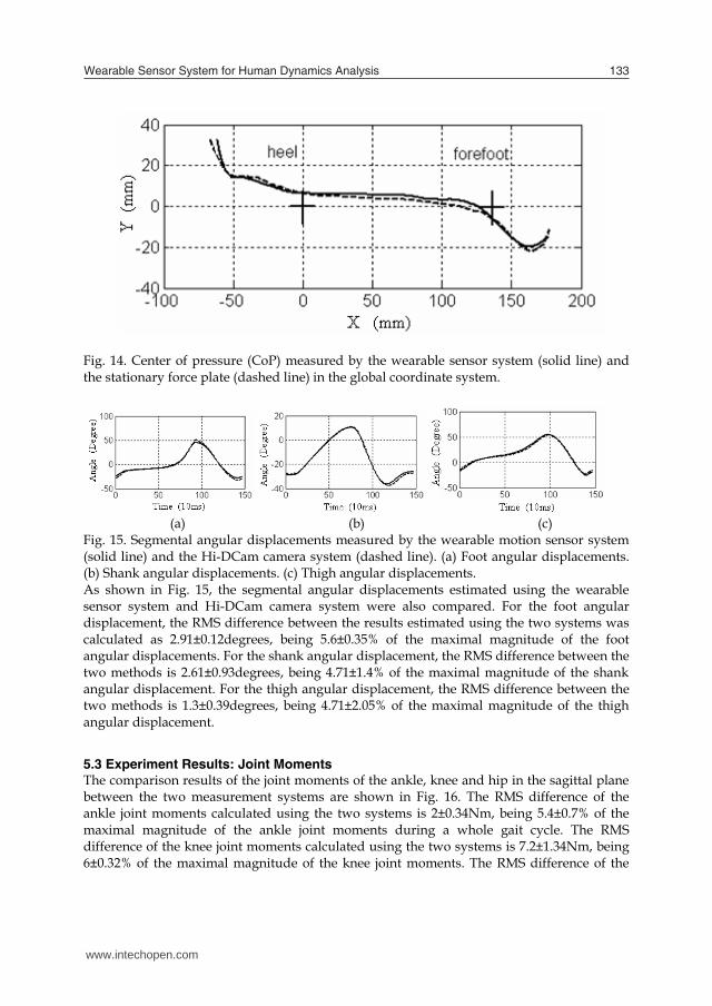
(d) (e) Fig. 13. Triaxial GRF measured by the wearable sensor systems (solid line) and the force plate (dashed line). (a) The vertical components: Fz. (b) The horizontal component: Fy. (c) Horizontal component: Fx. (d) The total GRF. (e) Error of GRF between the two measurement systems. The estimation of the position of the CoP is shown in Fig. 14. The trajectories agree well, and RMS difference between the two methods was 10.4±1.2mm, corresponding to 3.7±0.5% of the length of the instrumented shoe.
Fig. 14. Center of pressure (CoP) measured by the wearable sensor system (solid line) and the stationary force plate (dashed line) in the global coordinate system.
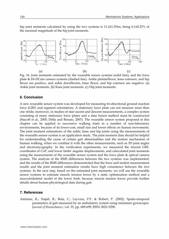
(a) (b) (c)
Fig. 15. Segmental angular displacements measured by the wearable motion sensor system (solid line) and the Hi-DCam camera system (dashed line). (a) Foot angular displacements. (b) Shank angular displacements. (c) Thigh angular displacements. As shown in Fig. 15, the segmental angular displacements estimated using the wearable sensor system and Hi-DCam camera system were also compared. For the foot angular displacement, the RMS difference between the results estimated using the two systems was calculated as 2.91±0.12degrees, being 5.6±0.35% of the maximal magnitude of the foot angular displacements. For the shank angular displacement, the RMS difference between the two methods is 2.61±0.93degrees, being 4.71±1.4% of the maximal magnitude of the shank angular displacement. For the thigh angular displacement, the RMS difference between the two methods is 1.3±0.39degrees, being 4.71±2.05% of the maximal magnitude of the thigh angular displacement.
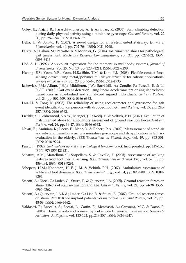
5.3 Experiment Results: Joint Moments The comparison results of the joint moments of the ankle, knee and hip in the sagittal plane between the two measurement systems are shown in Fig. 16. The RMS difference of the ankle joint moments calculated using the two systems is 2±0.34Nm, being 5.4±0.7% of the maximal magnitude of the ankle joint moments during a whole gait cycle. The RMS difference of the knee joint moments calculated using the two systems is 7.2±1.34Nm, being 6±0.32% of the maximal magnitude of the knee joint moments. The RMS difference of the
www.intechopen.com
Wearable Sensor System for Human Dynamics Analysis 133
The results show a good correspondence between two methods, which is confirmed by comparison analysis of the GRF (see Fig. 13(d)) and errors analysis of the GRF (see Fig. 13 (e)), and RMS differences by the ten subjects’ trials of 0.045±0.003 N/N (mean ± standard deviation), which corresponds to 4.26±0.34% of the maximal GRF magnitude. A separate analysis of each component of the GRF results for the vertical component in an RMS difference of 0.046±0.002N/N, being 4.8±0.2% of the maximal GRF magnitude, or 4.2±0.2% of the maximal vertical components. For the x-directional component of the horizontal GRF, RMS difference is 0.011±0.008N/N, being 1.07±0.91% to the maximal GRF magnitude, or 10.3±2.2% to the maximal x-directional component. For the y-directional component of the horizontal GRF, RMS difference is 0.014±0.002N/N, being 1.17±0.12% to the maximal GRF magnitude, or 10.1±3.6% to the maximal y-directional component of GRF.
(a) (b) (c)
(d) (e) Fig. 13. Triaxial GRF measured by the wearable sensor systems (solid line) and the force plate (dashed line). (a) The vertical components: Fz. (b) The horizontal component: Fy. (c) Horizontal component: Fx. (d) The total GRF. (e) Error of GRF between the two measurement systems. The estimation of the position of the CoP is shown in Fig. 14. The trajectories agree well, and RMS difference between the two methods was 10.4±1.2mm, corresponding to 3.7±0.5% of the length of the instrumented shoe.
Fig. 14. Center of pressure (CoP) measured by the wearable sensor system (solid line) and the stationary force plate (dashed line) in the global coordinate system.
(a) (b) (c)
Fig. 15. Segmental angular displacements measured by the wearable motion sensor system (solid line) and the Hi-DCam camera system (dashed line). (a) Foot angular displacements. (b) Shank angular displacements. (c) Thigh angular displacements. As shown in Fig. 15, the segmental angular displacements estimated using the wearable sensor system and Hi-DCam camera system were also compared. For the foot angular displacement, the RMS difference between the results estimated using the two systems was calculated as 2.91±0.12degrees, being 5.6±0.35% of the maximal magnitude of the foot angular displacements. For the shank angular displacement, the RMS difference between the two methods is 2.61±0.93degrees, being 4.71±1.4% of the maximal magnitude of the shank angular displacement. For the thigh angular displacement, the RMS difference between the two methods is 1.3±0.39degrees, being 4.71±2.05% of the maximal magnitude of the thigh angular displacement.
5.3 Experiment Results: Joint Moments The comparison results of the joint moments of the ankle, knee and hip in the sagittal plane between the two measurement systems are shown in Fig. 16. The RMS difference of the ankle joint moments calculated using the two systems is 2±0.34Nm, being 5.4±0.7% of the maximal magnitude of the ankle joint moments during a whole gait cycle. The RMS difference of the knee joint moments calculated using the two systems is 7.2±1.34Nm, being 6±0.32% of the maximal magnitude of the knee joint moments. The RMS difference of the
www.intechopen.com
Mechatronic Systems, Applications134
hip joint moments calculated by using the two systems is 11.2±1.3Nm, being 6.1±0.25% of the maximal magnitude of the hip joint moments.
(a) (b) (c) Fig. 16. Joint moments estimated by the wearable sensor systems (solid line), and the force plate & Hi-DCam camera systems (dashed line). Ankle plantarflexor, knee extensor, and hip flexor are positive, and ankle dorsiflexion, knee flexor, and hip extensor are negative. (a) Ankle joint moments. (b) Knee joint moments. (c) Hip joint moments.
6. Conclusion
A new wearable sensor system was developed for measuring tri-directional ground reaction force (GRF) and segment orientations. A stationary force plate can not measure more than one stride; moreover, in studies of stair ascent and descent measurements, a complex system consisting of many stationary force plates and a data fusion method must be constructed (Stacoff et al., 2005; Della and Bonato, 2007). The wearable sensor system proposed in this chapter can be applied to successive walking trials in a number of non-laboratory environments, because of its lower-cost, small size and lower effects on human movements. The joint moment estimations of the ankle, knee and hip joints using the measurements of the wearable sensor system is an application study. The joint moment data should be helpful for understanding the cause of certain gait abnormalities and the motion mechanism of human walking, when we combine it with the other measurements, such as 3D joint angles and electromyography. In the verification experiments, we measured the triaxial GRF, coordinates of CoP, and lower limbs' angular displacements, and caluculated joint moments using the measurments of the wearable sensor system and the force plate & optical camera system. The analysis of the RMS differences between the two systems was implemented, and the results of the RMS differences demonstrated that the force and motion measurement results and the joint moment estimation results have high consistence between the two systems. In the next step, based on the estimated joint moments, we will use the wearable sensor systems to estimate muscle tension forces by a static optimization method and a musculoskeletal model of the lower limb, because muscle tension forces provide further details about human physiological data during gait.
7. References
Aminian, K.; Najafi, B.; Bula, C.; Leyvraz, P.F. & Robert, P. (2002). Spatio-temporal parameters of gait measured by an ambulatory system using miniature gyroscopes. Journal of Biomechanics, vol. 35, pp. 689-699, ISSN: 0021-9290.
Coley, B.; Najafi, B.; Paraschiv-Ionescu, A. & Aminian, K. (2005). Stair climbing detection during daily physical activity using a miniature gyroscope. Gait and Posture, vol. 22 (4), pp. 287-294, ISSN: 0966-6362.
Della, U. & Bonato, P. (2007). A novel design for an instrumented stairway. Journal of Biomechanics, vol. 40, pp. 702-704, ISSN: 0021-9290.
Faivre, A.; Dahan, M.; Parratte, B. & Monnier, G. (2004). Instrumented shoes for pathological gait assessment. Mechanics Research Communications, vol. 31, pp. 627-632, ISSN: 0093-6413.
Hof, A. L. (1992). An explicit expression for the moment in multibody systems, Journal of Biomechanics, Vol. 25, No. 10, pp. 1209-1211, ISSN: 0021-9290.
Hwang, E.S.; Yoon, Y.R.; Yoon, H.R.; Shin, T.M. & Kim, Y.J. (2008). Flexible contact force sensing device using metal/polymer multilayer structure for robotic applications. Sensors and Materials, vol. 20, pp. 55-69, ISSN: 0914-4935.
Jasiewicz, J.M.; Allum, J.H.J.; Middleton, J.W.; Barriskill, A.; Condie, P.; Purcell, B. & Li, R.C.T. (2006). Gait event detection using linear accelerometers or angular velocity transducers in able-bodied and spinal-cord injured individuals. Gait and Posture, vol. 24, pp. 502-509, ISSN: 0966-6362.
Lau, H. & Tong, K. (2008). The reliability of using accelerometer and gyroscope for gait event identification on persons with dropped foot. Gait and Posture, vol. 27, pp. 248-257, ISSN: 0966-6362.
Liedtke, C.; Fokkenrood, S.A.W.; Menger, J.T.; Kooij, H. & Veltink, P.H. (2007). Evaluation of instrumented shoes for ambulatory assessment of ground reaction forces. Gait and Posture, vol. 26, pp. 39-47, ISSN: 0966-6362.
Najafi, B.; Aminian, K.; Loew, F.; Blanc, Y. & Robert, P.A. (2002). Measurement of stand-sit and sit-stand transitions using a miniature gyroscope and its application in fall risk evaluation in the elderly. IEEE Transactions on Biomed. Eng., vol. 49, pp. 843-851, ISSN: 0018-9294.
Parry, J. (1992). Gait analysis normal and pathological function, Slack Incorporated, pp. 149-158, ISBN: 9781556421921.
Sabatini, A.M.; Martelloni, C.; Scapellato, S. & Cavallo, F. (2005). Assessment of walking features from foot inertial sensing. IEEE Transactions on Biomed. Eng., vol. 52 (3), pp. 486-494, ISSN: 0018-9294.
Schepers, H.M.; Koopman, H. F. J. M. & Veltink, P.H. (2007). Ambulatory assessment of ankle and foot dynamics. IEEE Trans. Biomed. Eng., vol. 54, pp. 895-900, ISSN: 0018-9294.
Stacoff, A.; Diezi, C.; Luder, G.; Stussi, E. & Quervain, I.A. (2005). Ground reaction forces on stairs: Effects of stair inclination and age. Gait and Posture, vol. 21, pp. 24-38, ISSN: 0966-6362.
Stacoff, A.; Quervain, I.A.K.d.; Luder, G.; List, R. & Stussi, E. (2007). Ground reaction forces on stairs. Part II: Knee implant patients versus normal. Gait and Posture, vol. 26, pp. 48-58, ISSN: 0966-6362.
Valdastri, P.; Roccella, S.; Beccai, L.; Cattin, E.; Menciassi, A.; Carrozza, M.C. & Dario, P. (2005). Characterization of a novel hybrid silicon three-axial force sensor. Sensors & Actuators: A. Physical, vol. 123-124, pp.249-257, ISSN: 0924-4247.
www.intechopen.com
Wearable Sensor System for Human Dynamics Analysis 135
hip joint moments calculated by using the two systems is 11.2±1.3Nm, being 6.1±0.25% of the maximal magnitude of the hip joint moments.
(a) (b) (c) Fig. 16. Joint moments estimated by the wearable sensor systems (solid line), and the force plate & Hi-DCam camera systems (dashed line). Ankle plantarflexor, knee extensor, and hip flexor are positive, and ankle dorsiflexion, knee flexor, and hip extensor are negative. (a) Ankle joint moments. (b) Knee joint moments. (c) Hip joint moments.
6. Conclusion
A new wearable sensor system was developed for measuring tri-directional ground reaction force (GRF) and segment orientations. A stationary force plate can not measure more than one stride; moreover, in studies of stair ascent and descent measurements, a complex system consisting of many stationary force plates and a data fusion method must be constructed (Stacoff et al., 2005; Della and Bonato, 2007). The wearable sensor system proposed in this chapter can be applied to successive walking trials in a number of non-laboratory environments, because of its lower-cost, small size and lower effects on human movements. The joint moment estimations of the ankle, knee and hip joints using the measurements of the wearable sensor system is an application study. The joint moment data should be helpful for understanding the cause of certain gait abnormalities and the motion mechanism of human walking, when we combine it with the other measurements, such as 3D joint angles and electromyography. In the verification experiments, we measured the triaxial GRF, coordinates of CoP, and lower limbs' angular displacements, and caluculated joint moments using the measurments of the wearable sensor system and the force plate & optical camera system. The analysis of the RMS differences between the two systems was implemented, and the results of the RMS differences demonstrated that the force and motion measurement results and the joint moment estimation results have high consistence between the two systems. In the next step, based on the estimated joint moments, we will use the wearable sensor systems to estimate muscle tension forces by a static optimization method and a musculoskeletal model of the lower limb, because muscle tension forces provide further details about human physiological data during gait.
7. References
Aminian, K.; Najafi, B.; Bula, C.; Leyvraz, P.F. & Robert, P. (2002). Spatio-temporal parameters of gait measured by an ambulatory system using miniature gyroscopes. Journal of Biomechanics, vol. 35, pp. 689-699, ISSN: 0021-9290.
Coley, B.; Najafi, B.; Paraschiv-Ionescu, A. & Aminian, K. (2005). Stair climbing detection during daily physical activity using a miniature gyroscope. Gait and Posture, vol. 22 (4), pp. 287-294, ISSN: 0966-6362.
Della, U. & Bonato, P. (2007). A novel design for an instrumented stairway. Journal of Biomechanics, vol. 40, pp. 702-704, ISSN: 0021-9290.
Faivre, A.; Dahan, M.; Parratte, B. & Monnier, G. (2004). Instrumented shoes for pathological gait assessment. Mechanics Research Communications, vol. 31, pp. 627-632, ISSN: 0093-6413.
Hof, A. L. (1992). An explicit expression for the moment in multibody systems, Journal of Biomechanics, Vol. 25, No. 10, pp. 1209-1211, ISSN: 0021-9290.
Hwang, E.S.; Yoon, Y.R.; Yoon, H.R.; Shin, T.M. & Kim, Y.J. (2008). Flexible contact force sensing device using metal/polymer multilayer structure for robotic applications. Sensors and Materials, vol. 20, pp. 55-69, ISSN: 0914-4935.
Jasiewicz, J.M.; Allum, J.H.J.; Middleton, J.W.; Barriskill, A.; Condie, P.; Purcell, B. & Li, R.C.T. (2006). Gait event detection using linear accelerometers or angular velocity transducers in able-bodied and spinal-cord injured individuals. Gait and Posture, vol. 24, pp. 502-509, ISSN: 0966-6362.
Lau, H. & Tong, K. (2008). The reliability of using accelerometer and gyroscope for gait event identification on persons with dropped foot. Gait and Posture, vol. 27, pp. 248-257, ISSN: 0966-6362.
Liedtke, C.; Fokkenrood, S.A.W.; Menger, J.T.; Kooij, H. & Veltink, P.H. (2007). Evaluation of instrumented shoes for ambulatory assessment of ground reaction forces. Gait and Posture, vol. 26, pp. 39-47, ISSN: 0966-6362.
Najafi, B.; Aminian, K.; Loew, F.; Blanc, Y. & Robert, P.A. (2002). Measurement of stand-sit and sit-stand transitions using a miniature gyroscope and its application in fall risk evaluation in the elderly. IEEE Transactions on Biomed. Eng., vol. 49, pp. 843-851, ISSN: 0018-9294.
Parry, J. (1992). Gait analysis normal and pathological function, Slack Incorporated, pp. 149-158, ISBN: 9781556421921.
Sabatini, A.M.; Martelloni, C.; Scapellato, S. & Cavallo, F. (2005). Assessment of walking features from foot inertial sensing. IEEE Transactions on Biomed. Eng., vol. 52 (3), pp. 486-494, ISSN: 0018-9294.
Schepers, H.M.; Koopman, H. F. J. M. & Veltink, P.H. (2007). Ambulatory assessment of ankle and foot dynamics. IEEE Trans. Biomed. Eng., vol. 54, pp. 895-900, ISSN: 0018-9294.
Stacoff, A.; Diezi, C.; Luder, G.; Stussi, E. & Quervain, I.A. (2005). Ground reaction forces on stairs: Effects of stair inclination and age. Gait and Posture, vol. 21, pp. 24-38, ISSN: 0966-6362.
Stacoff, A.; Quervain, I.A.K.d.; Luder, G.; List, R. & Stussi, E. (2007). Ground reaction forces on stairs. Part II: Knee implant patients versus normal. Gait and Posture, vol. 26, pp. 48-58, ISSN: 0966-6362.
Valdastri, P.; Roccella, S.; Beccai, L.; Cattin, E.; Menciassi, A.; Carrozza, M.C. & Dario, P. (2005). Characterization of a novel hybrid silicon three-axial force sensor. Sensors & Actuators: A. Physical, vol. 123-124, pp.249-257, ISSN: 0924-4247.
www.intechopen.com
Mechatronic Systems, Applications136
Veltink, P.H.; Liedtke, C.; Droog, E. & Kooij, H. (2005). Ambulatory measurement of ground reaction forces. IEEE Trans Neural Syst Rehabil Eng., vol. 13, pp. 423–527, ISSN: 1534-4320.
Yavuzer, G., Oken, O., Elhan, A., Stam, H.J., 2008, “Repeatability of lower limb three-dimensional kinematics in patients with stroke,” Gait and Posture, 27(1), pp. 31-35, ISSN: 0966-6362.
Zatsiorsky, V. M. & Seluyanov, V. N. (1983). The mass and inertia characteristics of the main segments of the human body, In: Biomechanics VIII-B, Edited by Matsui, H. & Kobayashi, K., pp. 1152-1159. Human Kinetics Publishers, Chamapaign, IL.
Zhang, K.; Sun, M.; Lester, D.K.; Pi-Sunyer, F.X.; Boozer, C.N. & Longman, R.W. (2005). Assessment of human locomotion by using an insole measurement system and artificial neural networks. Journal of Biomechanics, vol. 38, pp. 2276-2287, ISSN: 0021-9290.
Zheng, R.; Liu, T.; Inoue, Y.; Shibata, K.; Liu, K.; (2008). Kinetics analysis of ankle, knee and hip joints using a wearable sensor system, Journal of Biomechanical Science and Engineering. Vol. 3(3), pp.343-355, ISSN: 1880-9863.
www.intechopen.com

Mechatronic Systems ApplicationsEdited by Annalisa Milella Donato Di Paola and Grazia Cicirelli
ISBN 978-953-307-040-7Hard cover, 352 pagesPublisher InTechPublished online 01, March, 2010Published in print edition March, 2010
InTech EuropeUniversity Campus STeP Ri Slavka Krautzeka 83/A 51000 Rijeka, Croatia Phone: +385 (51) 770 447 Fax: +385 (51) 686 166
InTech ChinaUnit 405, Office Block, Hotel Equatorial Shanghai No.65, Yan An Road (West), Shanghai, 200040, China
Phone: +86-21-62489820 Fax: +86-21-62489821
Mechatronics, the synergistic blend of mechanics, electronics, and computer science, has evolved over thepast twenty five years, leading to a novel stage of engineering design. By integrating the best design practiceswith the most advanced technologies, mechatronics aims at realizing high-quality products, guaranteeing atthe same time a substantial reduction of time and costs of manufacturing. Mechatronic systems are manifoldand range from machine components, motion generators, and power producing machines to more complexdevices, such as robotic systems and transportation vehicles. With its twenty chapters, which collectcontributions from many researchers worldwide, this book provides an excellent survey of recent work in thefield of mechatronics with applications in various fields, like robotics, medical and assistive technology, human-machine interaction, unmanned vehicles, manufacturing, and education. We would like to thank all the authorswho have invested a great deal of time to write such interesting chapters, which we are sure will be valuable tothe readers. Chapters 1 to 6 deal with applications of mechatronics for the development of robotic systems.Medical and assistive technologies and human-machine interaction systems are the topic of chapters 7 to13.Chapters 14 and 15 concern mechatronic systems for autonomous vehicles. Chapters 16-19 deal withmechatronics in manufacturing contexts. Chapter 20 concludes the book, describing a method for theinstallation of mechatronics education in schools.
How to referenceIn order to correctly reference this scholarly work, feel free to copy and paste the following:
Tao Liu, Yoshio Inoue, Kyoko Shibata and Rencheng Zheng (2010). Wearable Sensor System for HumanDynamics Analysis, Mechatronic Systems Applications, Annalisa Milella Donato Di Paola and Grazia Cicirelli(Ed.), ISBN: 978-953-307-040-7, InTech, Available from: http://www.intechopen.com/books/mechatronic-systems-applications/wearable-sensor-system-for-human-dynamics-analysis
www.intechopen.com

www.intechopen.com

© 2010 The Author(s). Licensee IntechOpen. This chapter is distributedunder the terms of the Creative Commons Attribution-NonCommercial-ShareAlike-3.0 License, which permits use, distribution and reproduction fornon-commercial purposes, provided the original is properly cited andderivative works building on this content are distributed under the samelicense.