Development of a Wearable Sensor System for Human Dynamics Analysis

Liu Tao

A dissertation submitted to Kochi University of Technology

in partial fulfillment of the requirements for the degree of

Doctor of Philosophy

Graduate School of Engineering Kochi University of Technology

Kochi, Japan

September 2006

D e v e l o p m

e n t o f a

W e a r a b l e S

e n s o r S y s t e m

f o r H u m

a n D y n a m

i c s A n a l y s i s L

iu T

ao

1

Development of a Wearable Sensor System for Human Dynamics Analysis

Liu Tao

A dissertation submitted to Kochi University of Technology

in partial fulfillment of the requirements for the degree of

Doctor of Philosophy

Special Course for International Students Graduate School of Engineering Kochi University of Technology

Kochi, Japan

September 2006

2

3

Abstract We live in an epoch of computerization for every field of life. Many researchers are hammering

at the developments of the biomedical sensor that should be compact and should not force the

wearer to leave the comfort zone. The cheaper and more comfortable human dynamics

analysis devices with multi-sensor combinations, including force sensitive resistors,

inclinometer, goniometers, gyroscopes and accelerometers, are continuously proposed for

using in gait phases analysis and human dynamics analysis.

The wearable sensor system we constructed uses a developed six-axis reaction force sensor to

measure ground reaction forces during human walking and uses some inertial measurement units

(gyroscope sensor and accelerometer) to collect data from the human motion of interest. We

developed two prototypes of six-axis wearable force sensor with parallel mechanism to measure

ground-reaction forces in human dynamics analysis. A parallel flexible mechanism was firstly

designed for sensing impact forces and moments. Finite element method (FEM) was conducted

for dimension optimization. Sensitivity of the load cells in the force sensor was improved by

distributing strain gages on the maximum strain positions. A compact electrical hardware system

including amplifiers module, conditioning circuits and a microcomputer controller was developed

and integrated into the force sensor. The first prototype of a six-axis force sensor was made to

validate the theory of parallel-mechanism. The mass of the sensor is about 300g, and its length,

width and height are 170mm, 105mm and 26.5mm respectively. A new parallel sensor was

developed based on the No.1 sensor prototype for the future human dynamics analysis. In order to

make the mechanism more compact, hybrid measurement load cells were adopted for X-and Y-

direction translational forced measurement. The new design can decrease the number of strain

gauges and amplifier modules. The mass of the entire sensor system is about 0.5 kg, and the

4

dimensions are 115 mm in length, 115 mm in width and 35 mm in height.

For the second portion of this study, two inexpensive human motion analysis systems were

constructed, in which gyroscopes (ENC-05EB) were used to measure angular velocities of body

segments, and two-axis accelerometers (ADXL202) were used to measure the accelerations for

the calibration in each human motion cycle. The first wearable sensor system is designed for only

foot motion analysis and the second system can be used for a leg (foot, shank and thigh) motion

analysis. Base on the two sensor systems, a fuzzy inference system (FIS) is developed for the

calculation of the gait phases derived from sensors’ outputs. A digital filter is also designed to

remove noises from the output of the fuzzy inference system, which enhances robustness of the

system. Finally, experimental study is conducted to validate the wearable sensor systems using an

optical motion analysis system.

At last, we combined the developed wearable human motion analysis sensor system with the

reaction force sensor worn under the foot to implement human dynamics analysis. The gait phase

division was performed to improve the precision of this method by providing constrain condition

about the functional muscles for an optimum analysis. We have completed the analysis

experiments to ten subjects (average age: 21, average height 1.7m). The quantitative analysis

results form the sensor system using direct integral calculation were compared with the data

obtained from a commercial optical motion analysis system and a referenced force plate.

5

Contents

Abstract…………………………………………………………3

1 Introduction…………………………………………………..9 1.1 Research Background and Historical Methods……………………9

1.2 Research Goals…………………………………………………….12

2 Wearable Force Sensor Systems……………………………..14 2.1 Summary…………………………………………………………..14

2.2 No.1 Sensor Prototype Design…………………………………….14

2.2.1 Parallel Support Principle……………………………………..15

2.2.2 Load-Cell Design…………………………………………......16

2.2.3 Sensor Mechanical Design……………………………………18

2.2.4 Amplifier and Recorder……………………………………….20

2.2.5 Calibration Experiments………………………………………20

2.3 No.2 Sensor Prototype Design…………………………………….23

2.3.1 Mechanical Design and Dimension Optimization…………….23

2.3.2 Electrical System Design……………………………………...27

2.3.3 Software Design……………………………………………….28

2.3.4 Calibration Experiments……………………………………....29

2.3.5 Coupling Effect Tests………………………………………….31

3 Wearable Motion Sensor Systems…………………………...35 3.1 Summary…………………………………………………………..35

6

3.2 Foot Motion Analysis System…………………………………….....36

3.2.1 Hardware Description……………………………………………36

3.2.2 Gait Phases………………………………………………………37

3.2.3 Fuzzy Inference System…………………………………………39

3.2.4 Digital Filter……………………………………………………..40

3.2.5 Sample data………………………………………………………41

3.3 Leg Motion Analysis System………………………………………..43

3.3.1 Motion Sensor Units………………………………………….....44

3.3.2 Calibration……………………………………………………....46

3.3.3 Gait Phase Detection Algorithm………………………………...49

3.3.4 Drift Errors Study……………………………………………….52

3.3.5 Intelligent Calibration Method for Reducing Drift……………..55

4 Validation Experiments……………………………………….61 4.1 Reference Analysis System…………………………………………61

4.1.1 Optical Motion Analysis Systems………………………………61

4.1.2 Force Plate……………………………………………………....62

4.2 Wearable Force Sensor System Validation…………………………64

4.3 Wearable Motion Sensor System Validation……………………….65

5 Human Low Limbs Dynamics Analysis………………………67 5.1 Reaction Force Measurements………………………………………68

5.2 Low Limbs Motion Analysis………………………………………..72

5.3 Combination of the Developed Two Sensor System………………..74

6 Conclusions……………………………………………………76 6.1 Summary…………………………………………………………….76

6.2 Future Work………………………………………………………….78

6.3 Future Applications………………………………………………….79

7

Reference…………………………………………………………………81

Appendix…………………………………………………………………86

Acknowledgements………………………………………………………116

8

9

Chapter 1

Introduction

1.1 Research Background and Historical Methods

The standard method for human motion analysis is optical motion analysis using

high-speed cameras to record human motion. The integration of three-dimension motion

measurement using multi-camera systems and reaction force measurement using force

plates has been successfully developed to track human body parts and perform dynamics

analysis of their physical behaviors in a complex environment. However, the optical

motion analysis method needs considerable working space and high-speed graphic signal

processing devices, and using this analysis method the devices are expensive, and

pre-calibration experiments and offline analysis of recorded pictures are especially

complex and time-consuming. Therefore, this method is limited to laboratory research

and can’t be used in everyday applications. Moreover, the human body is composed of

many highly flexible segments, and the upper-body motion of humans is especially

complicated in terms of accuracy calculations [1]-[3].

Thus, cheaper and more comfortable human dynamics analysis devices with multi-sensor

combinations, including force sensitive resistors, inclinometer, goniometers, gyroscopes

and accelerometers, were proposed for use in gait phases analysis and human motion

analysis [4]-[5].

Pressure sensors are widely used to estimate the distributed vertical ground reaction

10

forces and determine the loading pattern of the plantar soft tissue in the stance phase of

gait [6]-[8], but in these systems the effects of shearing forces are neglected. Some silicon

sensors recently are developed to measure both compressive and shear forces at the

skin-object interface [9]-[11], and the force levels of these sensors are limited in the

measurements of small forces (about 50N).

Two multi-dimensional sensors for human dynamics analysis have been introduced in [12]

and [13], and these sensors are made with serial structures, in which each load cell should

be strong enough to stand the loads originating from non-measurement directions.

Moreover the serial structure sensors with load-couple are difficult to be calibrated. Liu

proposed a six-axis sensor with four six-axis load cells distributed on four supporting

points, but the measurement ranges in the six-axis are never enough for human

reaction-force measurements [14]. A new force sensor with parallel support structure

developed by Nishiwaki can be used to measure the reaction forces during human

walking, and implement control algorithm of humanoid robots’ zero moment point (ZMP)

[15]. However, the proposed sensor (weight about 700 g) manufactured with the

hardened tool steel is a little heavy, which probably lead to comfortlessness while worn

under the human foot. Thus in the force sensor presented in this paper, we implement a

more compact mechanical design to combine load cells, and the material of hard

aluminum was used for fabricating load cells to decrease weight of sensor.

About the human motion analysis, many researchers have used single accelerometers or

multi-accelerometer combinations for daily human gait phase detection or assessment,

and these studies can find application in clinical and robotics research [16]- [21]. Gait

phase detection from accelerometer data was implemented to distinguish between stance

11

and swing phase [22], but large disturbances in the acceleration signal possibly affect real

time precision in the clinical applications. The quantitative analysis of human motion was

also investigated in [23], and by using assembled multi-axis accelerometer sensors, a

measurement system was made for estimation of three-dimensional position and

orientation of a body segment, but large estimate errors from offset error in the

accelerometer and inaccuracy in the orientation of the individual accelerometer’s active

axis make this system unsuitable for quantitative body segment motion analysis in

biomechanical applications.

Accelerometer signals do not contain information about rotation around the vertical axis

and therefore do not give a complete description of human motion. In [24], K. Tong and

H. M. Grant proposed a measurement device using two gyroscopes, one placed on the

thigh and the other on the shank, which can estimate knee rotation angle during walking.

This system can detect different phases of human walking, but the quantitative analysis of

leg motion was not completed in this study. Ion P.I. Pappas al. in [25] used a detection

system consisting of three force-sensitive resistors, which measure the force loads on a

shoe insole, and a gyroscope, which measures the rotational velocity of the foot. The

system detects the four gait phases accurately and reliably in real time, but it was only

designed for application to functional electrical stimulation.

A problem with the inertial sensors of gyroscopes and accelerometers is that they suffer

from a fluctuating offset, which results from temperature change or small changes in the

structure (mechanical wear). When accelerometers are used in clinical applications, a

complex calibration procedure is impractical and can cause misuse [26]-[27]. H. J.

Luinge proposed a Kalman filter that fuses tri-axial accelerometer and a tri-axial

12

gyroscope signals for ambulatory recording of human body segment orientation [28]-

[29]. It was reported that a filter based on three assumptions can continuously correct

offset errors from accelerometer outputs. However, as discussed in [30], if the Kalman

filter is applied to accelerometer measurements on the segments like arms or legs,

moving with large centripetal acceleration components, the inclination estimate will

probably be less accurate using an assumption that the acceleration of body segments in

the global system can be described as low pass filtered white noise.

1.2 Research Goals

The overall goal of this research project is to develop a wearable intelligent sensor system

for human dynamics analysis. The sensor system is composed of a wearable reaction

force sensor system and a wearable motion analysis sensor system. The claim is that this

sensor system will provide a lower-cost, more maneuverable and more flexible sensing

modality than those currently in use.

The first step in the framework is the wearable reaction force sensor system. The

traditional and commercial sensor usually adopts serial load cells structure, so each load

cell should be strong enough to stand the loads originating from non-measurement

directions. However, in the case of reaction forces during human walking, the gravity

direction forces may be over 1000N, and the friction forces are only about 50N. The large

landing impact and rotational forces of human moving make it difficult to find traditional

or commercial sensors for such application. A six-axis force sensor with parallel

mechanism is proposed to measure ground-reaction forces in human dynamics analysis

[31].

13

In the second step, a motion analysis system with intelligent calibration for leg segment

quantitative motion analysis of human walking is introduced. This motion analysis

system is the combination of three gyroscopes that measure the rotational velocity of the

foot, shank and thigh, and a two-axis accelerometer-chip that can detect two-directional

accelerations around the ankle during walking. An estimation algorithm based on

kinematic restriction of human walking was developed to continuously correct orientation

estimates, which obtained by mathematical integration of the angular velocity measured

by using gyroscopes. Gait analysis results including leg segment orientation obtained

with this motion analysis system are compared with the motion analysis results obtained

using a laboratory optical motion analysis system [32]-[33].

The last step is experimental study of combining the two sensor systems for human

dynamics analysis. Firstly, the sensor devices are worn on the subject’s leg to measure 2D

motion of leg (foot, shank and thigh) and six-axis reaction forces, and the sensors’ data is saved in

the pocketed data recorder. Secondly when the human motion and force record are finished, the

data in the data recorder is fed into personal computer through serial port (RS232), then walking

data is prepared for the offline motion analysis computing. Finally, the leg dynamics analysis is

performed to estimate the leg segments’ angular orientations and reaction forces.

Chapter 2 and chapter 3 will respectively discuss the design of the wearable force sensor

system and the wearable motion sensor system we created. Chapter 4 will introduce the

validation experiments of the two sensor systems, and Chapter 5 presents the human

dynamics analysis experiments on a group of subjects (average age: 21, average height

1.7m) wearing the developed sensor system. Chapter 6 presents the conclusions and

future directions.

14

Chapter 2

Wearable Force Sensor Systems

The wearable force sensor system is one main part of this project. It is provided the human

ground reaction forces data to the dynamics analysis software later processed. The design of the

force sensor system itself will be described in some detail, including the examination of the

parallel support principle, the sensor mechanical and electrical circuits design and calibration

experiments. The general operation of the sensor system in the experimental study will also be

explained. For readers not interested in the technical details, a short summary is also provided.

2.1 Summary

We developed two prototypes of six-axis wearable force sensor with parallel mechanism to

measure ground-reaction forces in human dynamics analysis. A parallel flexible mechanism was

firstly designed for sensing impact forces and moments. Finite element method (FEM) was

conducted for dimension optimization. Sensitivity of the load cells in the force sensor was

improved by distributing strain gages on the maximum strain positions. A compact electrical

hardware system, including amplifiers module, conditioning circuits and a microcomputer

controller, was developed and integrated into the force sensor.

2.2 No.1 Sensor Prototype Design

The first prototype of a six-axis force sensor was made to validate the theory of

parallel-mechanism. The X-, Y- and Z- directions represent leftward, forward and upward

direction respectively, meanwhile Mx, My and Mz represent three-direction moments. The mass

of the six-axis sensor is about 300g, and sensor’s length, width and height are 170 mm, 105 mm

15

and 26.5 mm respectively.

2.2.1 Parallel Support Principle The traditional and commercial sensors usually are made in serial load cells structure, so each

load cell should be strong enough to stand the loads originating from non-measurement directions.

However, in the case of reaction forces during human walking, the gravity direction forces may

be over 1000N, and the friction forces are only about 50N. When the force sensor is worn under

foot, the large landing impact and rotational forces of human moving make it difficult to find

traditional or commercial sensors for such application.

Figure 2-1 shows the measurement theory of the two kinds of support mechanisms. The sensor

with serial structure should be strong enough for each load cell to stand loads coming from

non-measurement directions. To stand large pressure force and rotational moment, parallel

support mechanism is used to distribute the reaction forces to many different support points. In

each support point, only translational forces are measure by load cells. The interference of

different direction forces can be neglected, because the relationship of measurement load cell and

input force is one-to-one.

The developed sensor with parallel support mechanism can detect moments in three directions,

through measuring translational forces in three directions on each support point. As show in Fig.

2-2, the sensor is mainly composed of four parts: top plane, bottom plane, load cell and balls.

When the forces including moments are applied on down plane, keeping mechanisms on the

down plane transfer the forces to four support balls, then through the contacting actions between

balls and load cells, three-axis translational forces on each support point are measured by load

cell. The strain gages on load cells are the sensing components.

16

Fig. 2-1 Sensor with Serial support mechanism and sensor with parallel support mechanism

Fig. 2-2 Sensor with parallel Support mechanism

2.2.2 Load-Cell Design

A group of load cells were designed to measure the translational force using strain gauges. On

each support point, three load cells are used to measure three-direction translational forces. Three

load cells are put on three support points respectively, and measure three-direction translational

forces, each load cell uses strain gauges to detect the translational force. As shown in Fig. 2-3, a

hard ball is adopted to transfer three-direction translational forces to load cell through point

contacts with three load cells. The contacting moment between ball and load cell is not included,

because the point contact of ball only transfer translational force. In order to decrease effect of

friction, high hard balls (SUJ Hardened high carbon-chrome steel, surface hardness HRC 62-67)

and hardened tool steel (SKD11 HRC 65) are used on the contacting points (Fig. 2-4).

Bottom plane

Top plane

Support ball Load cell

F F

Parallel support mechanism

Load cell

Serial support mechanism

17

Fig. 2-3 Three-axis load cell

Fig. 2-4 Load cell

We adopted finite element method to optimize the dimensions of the load cells. The solid model

of the beam in the load cell measuring Y- and Z- direction force was constructed by using

software of Pro/E, and imported to finite element analysis software of ANSYS to perform the

static force analysis of the beam. The resistant strain gauges are distributed on the position with

maximum strain according to the finite element analysis (FEA) result.

Fig. 2-5 3D model of beam

Support ball

Hardened tool steel

Force

Load cell

Support ball

Y

ZY load cell

Z load cell

X load cell

X

18

Fig. 2-6 Result graph of FEA

2.2.3 Sensor Mechanical Design Figure 2-7 shows the prototype of the wearable force sensor, in which the measurement beam was

made of ultra hard duralumin, and ten groups of resistant strain gages are used to construct the 12

load cells (see appendix Fig. C-1-C-7). In order to make the mechanism more compact, as show

in Fig. 2-8, hybrid measurement beam is adopted for Y, and Z direction load cell. This design also

can decrease the number of strain gauges and amplifier modules. The full rated force sets for this

sensor are specified to be Fx=Fy=20kgf, Fz=100kgf, and Mx=My=Mz=100Nm.

Fig. 2-7 Prototype of the six-axis force sensor

Mz

Fy

My

Mx

Fx

Fz

19

Fig.2- 8 Mechanism of hybrid beams

Figure 2-9 shows a simplified graph of six-axis measurement sensor. Assume six–dimension

force calculation point as the center of ball center’s plain. Force for positive direction of Fx is

measured as Fx1+Fx2, and negative direction as Fx3+Fx4. Therefore, Fx can be defined as follows:

4321 xxxxx FFFFF −−+= (1)

Fy and Fz can also be calculated in (2) and (3) by using the same method.

3241 yyyyy FFFFF −−+= (2)

3241 zzzzz FFFFF +++= (3)

Define L as the distance of support point along Y-axis direction, and W as the distance of support

point along X-axis direction. Then the rotation moments on center point can be calculated by

using the outputs of the load cells. Mx, My and Mz are calculated as follows;

2/)( 4132 LFFFFM zzzzx −−+= (4)

2/)( 2143 WFFFFM zzzzy −−+= (5)

2/)(2/)(

4231

4231

WyFFFFLFFFFM

yyy

xxxxz

−−++−−+=

(6)

20

Fig. 2-9 Calculation of six-axis force

2.2.4 Amplifier and Recorder In the experiment of the six-axis sensor, strain measurement device EDX-1500A of Kyowa

Electronic Instruments Co was used to amplify and record dynamic signals of strain gage in each

load cell (Fig. 2-10).

Fig. 2-10 Amplifier and recorder of load cell output

2.2.5 Calibration Experiments A three-direction drag mechanism was designed to calibrate the load cells in the parallel force

sensor, as show in Fig. 2-11. The load cell can be separately calibrated by using this mechanism,

because the parallel sensor was designed to make six-axis forces decouple, and interference

among different axes was decreased by the parallel support mechanism, which just measure

translational forces in three directions.

FX1

FY1 FZ1

FX4

FY4

FY2 FZ2

FY3

FX3

L

W FZ4

FX2

FZ3

EDX-1500A

21

(a)

(b)

(c)

Fig. 2-11 Calibration of the force sensor. (a) Calibration mechanism of the horizontal force load cells.

Sensor

Drag mechanism

Drag force (F)

Weight (G)

Horizontal load cell

Pulley

F=G

Weight (G)

Gravimeter

Vertical Load cell

Pressure force (F)

G0

F=G-G0

22

Reference force (drag force F) is produced through a pulley which transmits gravity of the weight to the

drag force on the load cell. (b) Calibration mechanism of the vertical force load cells. A gravimeter is used

to measure applied vertical force on the load cell.

Referenced forces were applied on every load cell, and outputs of load cells were recorded by

strain measuring device (KYOWA EDX-1500A). Method of least square was used to calculate

calibration coefficient in MATLAB. The calibration graphs of X-, Y- and Z-axes are shown in Fig.

2-12, Fig. 2-13 and Fig. 2-14 respectively. In the calibration graphs, the vertical axis represents

input forces of load cell, and the horizontal axis represents output of load cells.

Fig. 2-12 X-direction calibrations

Fig. 2-13 Y-direction calibrations

23

Fig. 2-14 Z-direction calibrations

As show in table I, X-, Y- and Z-directions forces calibration matrices are defined as [Cx1, Cx2],

[Cy1, Cy2, Cy3, Cy4], [Cz1, Cz2, Cz3, Cz4] respectively.

TABLE I. CALIBRATION COEFFICIENT OF TEN DIRECTIONS

Calibration Coefficient X(*10-3) Y(*10-3) Z(*10-3)

Cx1 Cx2 Cy1 Cy2 Cy3 Cy4 Cz1 Cz2 Cz3 Cz4

2.8 2.7 2.7 2.8 2.7 2.4 7.0 6.3 6.5 6.2

2.3 No.2 Sensor Prototype Design

In study of the No.1 sensor prototype, we had made a parallel six axis force sensor with simple

structure to validate the theory of this new kind of structure in the design of the sensor design. A

new parallel sensor was developed based on the No.1 sensor prototype for the future human

dynamics analysis. In order to make the mechanism more compact, hybrid measurement load

cells were adopted for X-and Y- direction translational forced measurement. The new design can

decrease the number of strain gauges and amplifier modules. The mass of the entire sensor system

is about 0.5kg, and the whole dimensions are 115mm in length, 115mm in width and 35mm in

height.

2.3.1 Mechanical Design and Dimension Optimization

24

As shown in Fig. 2-15, the sensor is composed of the bottom plane, X-, Y- and Z- load cells, and

the balls (see appendix Fig C-8-C-C-12). When the forces and the moments are applied on the

bottom plane, they are transferred onto the four support balls. The supprt balls are connected with

the three load cells by ponit contacts. Therefore, only translational forces are transferred to the

corresponding load cells, and are measured by the strain gauges attached on the load cells. The

X-load cell can measure FX1 and FX2. Similarly, the Y-load cell measures FY1 and FY2, and the

Z-load cell measures FZ1, FZ2, FZ3 and FZ4. Based on these measured values, the three-axis forces

and moments can be calculated as following equations.

21 xxx FFF += (7)

21 yyy FFF += (8)

3241 zzzzz FFFFF +++= (9)

2/)( 4132 LFFFFM zzzzx −−+= (10)

2/)( 2143 LFFFFM zzzzy −−+= (11)

2/)( 1122 LFFFFM yxyxz −−+= (12)

25

Fig. 2-15 Schematic picture for the new Sensor with parallel Support mechanism. The x-, y-load cell is

composed of two x-load cells to measure Fx1 and Fx2 and two y-load cells to measure Fy1 and Fy2,

respectively. The z-load cells under the four support ball at the corners of L*L (L=100mm) can measure

four z-direction forces: Fz1, Fz2, Fz3 and Fz4.

Figure 2-16 shows the detail of the load cell. Each two strain gauges are attached on the load cell

to sense one-axis translational force. In order to obtain high sensitivity, the strain gauges should

be distributed on the points where maximum strains occur. ANSYS, FEA software, was used to

perform the static analysis of the load cell. Based on the sensitivity limitation of the strain gauge,

the optimal dimensions of the load cell were determined by ANSYS simulation. Figure 2-17

shows the results of the static analysis for the load cell.

26

Fig. 2-16 Schematic load cell. We put two strain gauges on each load cell mechanical structure, and a set of

two strain gauges is only sensitive to single direction translational force.

Fig. 2-17 Result graph of FEA. Finite element method was adopted to optimize the mechanism dimension

of strain beams, and improve the sensitivity of force sensor.

As shown in Fig. 2-18, based on the single load cell obtained by the optimal design mentioned in

the above section, the 3D structure is configured. Figure 2-19 shows the prototype of the load

cells in the wearable force sensor, and the flexible beams were made of ultra hard duralumin.

Four groups of the strain gauges were used to construct the x-, y-load cell, and another four

groups were used to construct the z-load cell. In order to make the mechanism more compact,

hybrid measurement load cells were adopted for X-and Y- direction translational forced

Strain gauges Normal force

Shear force Strain gauges

27

measurement. The new design can decrease the number of strain gauges and amplifier modules.

Fig. 2-18 3D model of the force sensor using the stimulation model of the force sensor, we designed the

mechanical structure of the parts in the sensor.

Fig. 2-19 Mechanical structure of the load cells. (a) The mechanical structure of z-load cell with four

sub-load cells which can measure z-direction vertical forces at the four support points. (b) The picture of

the x-, y-load cell for the measurements of the horizontal forces.

2.3.2 Electrical System Design and Integrated Sensor System

As shown in Fig. 2-20, an integrated electrical system was developed and incorporated into the

force sensor. The strains due to the forces applied on the flexible beam were converted to the

28

resistance changes. Then the resistance changes were converted to the voltage signals by the

conditioning modules, and were amplified by the amplifier modules. The amplified voltage

signals Xi were input into PC after A/D conversion. Since eight channels of the strain gauges

were used (four groups for X- and Y- direction force and another four groups Z-direction forces),

there were eight channels of the voltage signals. The program developed specially was used to

sample the eight channels of the voltage signals, and calculate the force and the moments (see

appendix Fig, C-13-C14) .

Fig. 2-20 Electrical hardware system of the sensor

The amplifier modules, conditioning circuits and microcomputer system were integrated on a based board,

which was fixed in the mechanical structures of the sensor. The outputs of the amplifiers and conditioning

modules (Xi) were used to calculate six-axis force applied on the sensor.

2.3.3 Software Design In order to achieve high signal to noise ratio, amplifier modules, conditioning circuits and

interface program were integrated into the force sensor. The large resistance strain gages (5000

29

ohm) of Vishay Micro-measurements were used, so the sensor system is low power consumed

and can be powered by using battery. Figure 2-21 shows the integrated sensor system and the

interface program developed specially for monitoring the data from the sensor.

Fig. 2-21 Sensor system with mechanical system, electrical system and software computing system. (a) The

sensor hardware system can be power using a battery and communicate with personal computer through

serial port of a Microcomputer system; (b) The software interface for the operation of senor and monitoring

the data from the sensor.

2.3.4 Calibration Experiments

In order to calibrate the developed sensor system, EFP-S-2KNSA12, a six-axis force and moment

sensor was used as the reference sensor. These two sensor systems worked in the synchronized

mode. The experimental system was established as shown in Fig. 2-22. It was mentioned above

that there were eight channels of the voltage signals Xi (I=1, … 8). Based on X1, …X8, the forces

and the moments can be calculated as the following equations.

. ∑=

=8

7iiix XAF

(13)

∑=

=6

5iiiy XAF

(14)

∑=

=4

1iiiZ XAF (15)

30

22

4

1

3

2

LXAXAMi

iii

iix

−= ∑∑

== (16)

2

2

1

4

3

LXAXAMi

iii

iiy

−= ∑∑

== (17)

−= ∑

=

+

2)1(

8

5

1 LXAMi

iii

z

(18)

where the Xi is the load cells’ conditioning outputs, and Ai is the calibration coefficients for each

load cells.

A multiple regression analysis was used for the calculation of the calibration coefficients. In this

study, we finished multiple regression analysis of the data using the statistical software of SPSS

11.0J. Fig. 2-23 present the graphs of the data, which imported into the multiple regression

analysis in SPSS. The results of the multiple regression analysis are shown in table II, and the

column Ai of calibration coefficients were used for the experimental study on the developed

sensor.

Fig. 2-22 Calibration experimental system

The force plate of Kyowa was used for the calibration of our developed sensor. This product

sensor can measure three direction forces and three direction moments in the center point.

31

Fig. 2-23 Calibration data from the two sensor systems. The synchronized measurement data of the

developed sensor and the product force plate was used for multiple regression analysis to calculate the

calibration coefficients of the load cells. (a) shows the load cells outputs of z-load cell (x1, x2, x3 and x4),

and (b) is the data of the product force plate for the measurements of the vertical forces.

Table II Calibration coefficients of the sensor

Load cell Unstandardized

coefficients

Standardized

coefficientsSig.

Ai Std. Error Beta

t

Z-Load cell 1 22.35 10.683 0.253 23.454 0.00

Z-Load cell 2 22.04 10.325 0.202 21.011 0.00

Z-Load cell 3 15.13 7.519 0.224 33.114 0.00

Z-Load cell 4 20.00 4.180 0.538 65.965 0.00

X-Load cell 1 28.15 2.650 -0.718 -87.079 0.00

X-Load cell 2 26.30 5.693 3.708 44.835 0.00

Y-Load cell 1 28.94 17.945 0.274 22.157 0.00

Y-Load cell 2 31.84 3.699 0.779 63.139 0.00

2.3.5 Coupling Effect Tests

Coupling effect tests have been performed to evaluate the interference errors of the sensor using

purposely-developing equipments. The test apparatus is shown in Fig. 2-24 and consists of clamp

device, loading device from a pulley mechanism and weights. Typical sensor load cells outputs, in

terms of voltage change versus loading force; in responding to loading on the three-axial load

32

cells (Fx, Fy and Fz) are plotted in Fig. 2-25. The effect of loading in one axis on the other load

cells was examined and minor fluctuations were observed. The interference errors of this sensor

were evaluated according to the results of cross-sensitivity test. The cross-sensitivity can be

expressed as the force measured on the load cells, which are normal to the testing direction load

cells. When the sensor was tested in X-direction, the cross-sensitivity for Y- and Z- directions was

calculated as 3.03% and 3.08%. While the test were being carried out on Y- and Z- directions, the

cross-sensitivity was calculated as 9.01% and 6.15%, and 0.14% and 0.10%, respectively (Table

III).

Fig. 2-24. Coupling effect tests. (a) Schematics of drag equipment for the calibration of x- and y- axis load cells. We adopted the same drag mechanism to produce horizontal reference forces in the test of x- and y-

33

load cells. (b) Schematics of normal force calibration equipment. We directly put weights on the sensor as a reference force to calibrate z-axis load cells, which measure normal direction force. (c) Experimental equipments picture.

Force (Kgf)

Out

put v

olta

ge (m

V)

(b)

Out

put v

olta

ge (m

V)

(a) Force (Kgf)

34

Fig. 2-25. Loading response of the three-axis load cells. (a) X-load cells. (b) Y-load cells. (c) Z-load cells.

Table III Results of interference errors test

Axes Load (Kgf) Average interference errors (%)

X Y Z

Fx 0-10 3.03 3.38

Fy 0-10 9.01 6.15

Fz 0-39 0.14 0.1

Out

put v

olta

ge (m

V)

Force (Kgf) (c)

35

Chapter 3

Wearable Motion Sensor Systems

In this study, two inexpensive human motion analysis systems were constructed, in which

gyroscopes (ENC-05EB) are used to measure angular velocities of body segments, and two-axis

accelerometers (ADXL202) are used to measure the accelerations for the calibration in each

human motion cycle. The design of the motion sensor system itself will be described in some

detail, including gyroscope and accelerometer calibrations; electrical boards design and an

intelligent calibration method. The general operation of the sensor system in the experimental

study will also be explained. For readers not interested in the technical details, a short summary is

also provided.

3.1 Summary

In this study, two inexpensive human motion analysis systems were constructed, in which

gyroscopes (ENC-05EB) are used to measure angular velocities of body segments, and two-axis

accelerometers (ADXL202) are used to measure the accelerations for the calibration in each

human motion cycle. The first wearable sensor system is designed for only foot motion analysis

and the second system can be used for a leg (foot, shank and thigh) motion analysis. Base on

the two sensor systems, a fuzzy inference system (FIS) is developed for the calculation of the gait

phases derived from sensors’ outputs. A digital filter is also designed to remove noises from of the

output of the fuzzy inference system, which enhances robustness of the system. Finally,

experimental study is conducted to validate the wearable sensor systems using an optical motion

analysis system.

36

The gait analysis system performs the detection of gait phases by using two types of inertial

sensors, i.e., two gyroscopes used to measure angular velocities of two-axis on the foot plane

during walking, and a two-axis accelerometer used to measure total transmission accelerations

including gravity acceleration and dynamic acceleration along two sensitive axes. The sensor

signals were sampled at a frequency of 100Hz with a resolution of 14 bits through A/D card

(Keyence NR-110), and the sample data is saved into the person computer for the analysis. The

card is connected with computer through micro-card interface of PCMCIA2.1 in personal

computer.

3.2 Foot Motion Analysis System

3.2.1 Hardware Description As shown in Fig. 3-1, an electrical base board was designed for the inertial sensor system. Two

miniature gyroscopes (Murata ENC-03J, size 15.5×8.0×4.3 mm, weight 10 g) are integrated on the

base board with their sensing axis oriented on the bottom plane of the foot respectively. The two

gyroscopes can measure two-dimension rotations of the foot in that plane. The Murata ENC-03J

gyroscope measures the rotational velocity by sensing the mechanical deformation caused by the

Coriolis force on an internal vibrating prism. The gyroscope signal is filtered by a third-order

band-pass filter (0.25–25 Hz) with a 20-dB gain in the pass band. The frequencies outside the

pass-band were filtered out because they are not related to the walking kinetics. The filtered gyroscope

signal was used to directly estimate the angular velocity of the foot and it was integrated to estimate

the inclination of the foot relative to the ground. The accelerometer-chip (ADXL202) with almost the

same theory as gyroscope-chip was fixed on the back of the base board, which can measure two-axis

accelerations including gravity acceleration and dynamic acceleration during walking. In the design of

data record device, the sampling time of A/D module is selected according to the bandwidth of signals,

and the sampling frequency should be higher than 2×1.25×25 Hz (the bandwidth of the inertial

sensors’ signals is about 25 Hz). Therefore the sensor signals were sampled at a frequency of 100

Hz>62.5 Hz with a resolution of 14 bits through A/D card (Keyence NR-110), and the sample data is

37

saved into the person computer for the analysis. The card is connected with computer through

micro-card interface of PCMCIA2.1 in personal computer. Because the two kinds of inertial sensors

are low energy consumed electrical devices, the motion analysis system is powered by using two

button batteries (CR2032), which can work up to 30 minutes in walking experiments (see appendix

Fig. C-15-C-16).

A mechanical shoe was designed to fix the base board of inertial sensors (Fig. 3-2). The foot

plane is parallel to the base board. The material was selected as Aluminum, and the weight is

about 500 g, the size is almost the same as common shoes.

(a) Front of the board (b) Back of the board

Fig. 3-1 Base board of the sensor system

Fig. 3-2 Hardware device of the motion anlysis system

3.2.2 Gait Phases In this paper, a normal walking gait cycle is divided into four different gait phases, i.e., stance,

toe-rotation, swing, and heel-rotation. The following is the definition of the gait phases (see Fig.

3-3): let stance phase be the period when the foot is with its entire length in contact with the

ground; let toe-rotation phase be the period following the stance phase during which the front part

38

of the foot is in contact with the ground and its heel is rotating around toe joint; let swing phase

be the period when the foot is in the air (not in contact with the ground); let heel-rotation phase be

the period following the swing phase which begins with the first contact of the foot with the

ground (usually the heel, but not necessarily) and the front part of foot is rotating around heel’s

contacting point, which ends when the entire foot touches the ground.

We define a walking cycle as the period from one stance phase of the foot to the next stance phase

of the same foot. In gait phase analysis algorism, these gait phases were represented by a

mathematics method with four distinct value ranges. The loop frequency of the phase record was

100 Hz, i.e., equal to the sensors sampling frequency.

Fig. 3-3 Transition of four gait phases

Physics sense analysis of each phase was performed to prepare design rules for the gait phase

detection algorithm. As shown in Fig. 3-4, when the motion measure device wears under the foot,

we suppose the subject is viewed from the lateral side and clockwise rotations are considered

positive. The Z- axis is vertical to the foot plane, and X- axis and Y- axis are along length- and

wide- orientations of foot respectively. The symbols ωx and ωy represent the rotational velocity of

foot around X- axis and Y- axis respectively. Physics senses of each phase can be defined as

following:

Toe-rotation Swing

Stance

Walking cycle

Heel-rotation

39

1). If ωx=0 AND ωy =0 AND Ax=0 AND Ay=0 Then ‘Stance Phase’;

2). If ωy<0 AND Ax≠0 AND Ay≠0 Then ‘Swing Phase’;

3). If ωy>0 AND Ax≠0 AND Ay≠0 Then If the case is before the ‘Swing Phase’ of the same

walking cycle Then ‘Toe-rotation Phase’ Else ‘Heel-rotation Phase’.

Fig. 3-4 Wearable motion analsys mechanical device

3.2.3 Fuzzy Inference System When the experiments data are recorded in the hard disk of personal computer, the off-line

analysis is made to analyze the gait during walking. The inertial sensors output signals are easy to

be affected by interrupts from testing environmental noise, and the static float of the inertial

sensors can decrease the precision of the measurements in the case of long time testing, so in the

study, a fuzzy inference system (FIS) is proposed to improve precision of the detection of gait

phase. The fuzzy system is robust to the noise from the inertial sensors. We design the fuzzy

inference system by using software of MATLAB (see Fig. 3-5). The two gyroscopes’ outputs and

the accelerometer’s two-axis outputs are defined as the four inputs of the FIS, and the output of

FIS is a value of gait phases.

In the design of fuzzy inference system, Mamdani fuzzy inference method was used as the

inference method. Each fuzzy input was defined as three fuzzy ranges: negative, zero and positive

(see Fig. 3-6), and each fuzzy range was designed by using saw-tooth function. In the same way,

the output of FIS was defined as four fuzzy ranges to de-fuzzy inference results in the Mamdani

method. As shown in Fig. 3-7, the four output ranges is named as: stand, toe-r, swing, and heel-r

40

respectively.

Fig. 3-5 Theory schematics of theFIS

Fig. 3-6 Fuction of fuzzy input

Fig. 3-7 De-fuzzy output of the FIS

3.2.4 Digital Filter In this section, a digital filer designed for the outputs of FIS is presented. The inertial sensors are

sensitive to the environmental noise, which leads to the difficulty of detecting the gait phases

precisely using a simple algorithm in a micro-computer. To get the decided gait phases change

points of human walking, a digital filter is used to remove noise results from the fuzzy inference

system. We recorded the inertial sensor system’s signals at a frequency of 100Hz, and the normal

human walking period is about 1.5 sec, so in the results of Firsthe pulse interrupts with period of

no over 0.05 sec can be confirmed as the errors pulses in the gait phase detection. A digital filter

was designed to filter the error pulses in the results of FIRSThe symbols R(i) and Rf(i) represent

41

the output result of FIS and last filtered results on the i-th sampling cycle (i=2,3,4…), and k

represents the noise pulse swing value. Then the rule of the filter is designed as follows. If the

absolute value of R(i-1) subtracted by R(i+3) is far no more than k, and one of the absolute

value among R(i) subtracted by R(i-1) , R(i+1) subtracted by R(i-1) and R(i+2) subtracted by

R(i-1) is larger than k, then the value of R(i), R(i+1) and R(i+2) is set as the same value as R(i-1),

because in this case the 50ms sampling range (from i-1 to i+3) must be added in a noise pulse

(see Fig. 3-8).

Fig. 3-8 Theory of the digital filter

3.2.5 Sample data An experimental study was carried out in order to quantify that the motion analysis system can be

used on normal gait phases detection for the future motion analysis study. The study involved a

group of healthy adults who worn the special mechanical shoes on the one foot. The inertial

sensors’ data were recorded in the personal computer through the A/D card with resolution of 14

bits. All the subjects walked on a plane ground (length = 30 m), and their gait cycle is about 1.5s.

The gait phases were analyzed off-line based on the data from the two kinds of inertial sensors.

After calibrated to be zero when no motion and adjusted to change from -2.5 to 2.5 in the same

range, the four-output data from inertial sensors were fed into the fuzzy inference system

according to sampling time cycle. As shown in Fig. 3-9, one subject’s motion data were recorded

42

about using x- axis gyroscope, y- axis gyroscope, x- axis accelerometer, y- axis accelerometer

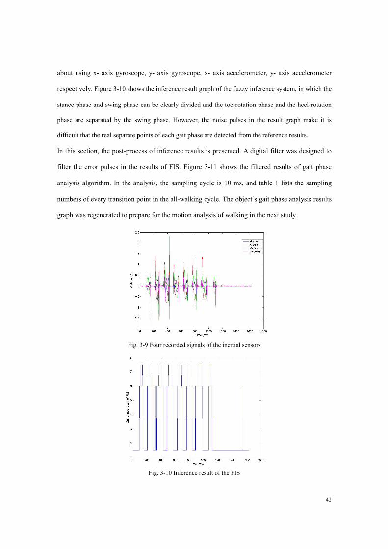
respectively. Figure 3-10 shows the inference result graph of the fuzzy inference system, in which the

stance phase and swing phase can be clearly divided and the toe-rotation phase and the heel-rotation

phase are separated by the swing phase. However, the noise pulses in the result graph make it is

difficult that the real separate points of each gait phase are detected from the reference results.

In this section, the post-process of inference results is presented. A digital filter was designed to

filter the error pulses in the results of FIS. Figure 3-11 shows the filtered results of gait phase

analysis algorithm. In the analysis, the sampling cycle is 10 ms, and table 1 lists the sampling

numbers of every transition point in the all-walking cycle. The object’s gait phase analysis results

graph was regenerated to prepare for the motion analysis of walking in the next study.

Fig. 3-9 Four recorded signals of the inertial sensors

Fig. 3-10 Inference result of the FIS

43

Fig. 3-11 Filtered inference result of the FIS

TABLE II. GAIT PHASES TRANSITION POINTS OF AN OBJECT

Transition points(Sampling cycle number) Gait phases transition Walking

cycle number Stance to

Toe-r Toe-r to Swing

Swing to Heel-r

Heel-r toStance

1 94 107 137 158

2 206 228 269 285 3 342 365 408 430 4 480 501 547 567

5 628 649 687 705 6 755 774 817 836 7 884 911 957 979

8 1065 1077 1097 1112

3.3 Leg Motion Analysis System

Based on the first wearable sensor system (foot motion analysis system) and its experimental

study, second wearable sensor system for the whole leg (foot, shank and thigh) motion analysis is

developed. This second system can be used for synchronous analysis of foot motion analysis,

shank motion analysis and thigh motion analysis, in which a new inertial sensor combination and

special data-recorder are designed.

The wearable sensor system was made including an eight-channel data recorder, a gyroscope and

44

accelerometer combination module and two gyroscope modules. We attach the two gyroscope

modules on the foot and shank respectively, and the gyroscope and accelerometer combination module

is place on the thigh. The data recorder can be pocketed by the experimental object. A testing

experiment is finished for the second sensory system on measurement of leg motion during normal

walking. We use the same method introduced in the first sensory system’s study. In every stance phase

of walking cycle, the calibration is implemented to let initial integral constant be zero.

3.3.1 Motion Sensor Units As shown in Fig.3-12, three gyroscopes are used to measure angular velocities of leg segments of

foot, shank and thigh ( 1ω , 2ω and 3ω ). The sensing axis is vertical to the medial-lateral plane so

that the angular velocity in the sagittal plane can be detected. In local coordinates of three

segments, sensing axis of the gyroscopes is along y-axis, and the z-axis is along leg-bone. A

two-axis accelerometer is attached on the side of shank to measure two-direction accelerations

along tangent direction of x-axis ( ta ) and sagittal direction of z-axis ( ra ). In this system the data

from accelerometer are fused with data collected from gyroscopes for cycle system calibration,

through supplying initial angular displacement of the attached leg segment.

As shown in Fig. 3-13, the wearable sensor system includes an eight-channel data recorder, a

gyroscope and accelerometer combination unit and two gyroscope units. The two gyroscope units

are attached on foot and thigh respectively, and the gyroscope and accelerometer combination

unit is located on shank, which is near to ankle. The data recorder can be pocketed by the subject.

The principle operation of the gyroscope is the measurement of the Coriolis acceleration, which is

generated when a rotational angular velocity is applied to the oscillating piezoelectric bimorph.

The inertial sensor can work under low energy consumption (4.6 mA at 5V), and are appropriate

for ambulatory measurements. The signal from the gyroscopes and accelerometer are amplified

and low-pass filtered (cutoff frequency: 25Hz) to remove electronic noise. The frequencies

outside the pass-band are filtered out because they are invalid in study of human kinetics.

45

Fig. 3-12 Position and coordinates of the sensor unitsIn the local orientation coordinate of the sensor unit

(X-, Y- and Z- axis), Y-axis denotes each joint’s rocker axis, which is parallel to the sensitive axis of the

gyroscope, while X-axis and Z-axis denote the unity vectors in the radial and tangential direction,

respectively.

Fig. 3-13 Hardware system of the sensor system. A strap system is designed for the binding between the

sensor units and human body. The sensor unit is attached to the strap. During walking, the strap is tied

around the limb to secure the position of the sensor unit (see appendix Fig. C-17-C-21).

Sensor unit II on the shank

Sensor unit III on the thigh

Sensor unit I on the foot

Multi-channel Data- recorder

x

y z x

yz

x

Toe joint

Ankle joint

Knee joint

z y

Sensor unit I: Single-axis gyroscope sensitive to y- pitch velocity

Sensor unit II: Single-axis gyroscope and two-axis Accelerometer for shank motion

Sensor unit III: Single-axis gyroscope sensitive to y- pitch velocity

46

The multi-channel data-recorder is specially designed for the wearable sensor system. A

microcomputer (PIC 16F877A) is used to develop the pocketed data recorder, and sampling data

from the inertial sensors can be saved in a SRAM, which can keep recording for five minutes. An

off-line motion analysis (see appendix D) can be performed by feeding data saved in the SRAM

to a personal computer through a RS232 communication module. Since gyroscope (ENC-03J),

accelerometer-chip (ADXL202) and PIC system are all devices of low energy consumption, the

wearable sensor system is powered by using a battery of 300mAh (NiMH 30R7H).

3.3.2 Calibration Complete architecture of a calibration system is showed in Fig. 3-14(a), and hardware devices of

the system mainly include A/D card (Keyence NR-110), a potentiometer, a reference angle finder

and a clamp (Fig. 3-14(b)).

(a)

(b)

Fig. 3-14 (a) Architecture of the equipment for the calibration of the sensor unit. Two-axis accelerometer is

0°

90°

180°

gPotentiometerClamp

45°

at

ar

Reference angle finder

Sensor unit

ωat, ar, ωpθ

47

used to measure two-direction accelerations of at and ar, and pθ is output signal of the potentiometer which

measures imposed rotational quantities and provides reference angular velocity quantities through

difference computing. Signal of gyroscope in the sensor unit is defined as ω, and its positive direction is

anticlockwise. The four signals of pθ, ω, at and ar are sampled into computer through a 12-bit A/D card. (b)

Hardware devices with mechanical case and interface for the calibration of the sensor unit.

The sensor units are calibrated in two states of static and dynamic. The calibration of the

accelerometer sensor is carried out during the static state. The accelerometer in sensor unit is

subjected to different gravity vectors by rotating a based axis, which is connected with a

potentiometer. The dynamic calibration is completed to calibrate the gyroscopes and test the

accelerometer in a moving condition. In both cases the calibration matrixes are computed using

the least squares method.

[ ]θC is calibration matrix for the angle position (3-1), where [ ]θ is the matrix of the imposed

quantities, which in this specific case were obtained when the sensor unit is rotated to different

positions on the angle finder plane; [ ]θp is the matrix of the quantities acquired from the

potentiometer, in the specific sensor unit positions. Angular position [ ]rθ can be calculated

using (3-2), and angular velocity of the sensor unit is obtained through difference computing of

the angular positions in serial time. Gravity g subjected to the two sensitive axis (at and ar) of the

accelerometer is estimated in (3-3) and (3-4).

[ ] [ ][ ] [ ][ ] 1)( −= TT pppC θθθθ θ (3-1)

[ ] [ ] [ ]θθθ pCr ⋅= (3-2)

)cos( rt gA θ⋅−= (3-3)

)sin( rr gA θ⋅−= (3-4)

48

[ ]atC and [ ]arC are calibration matrixes for the two-axis accelerometer (3-5) (3-6), where [ ]tA

and [ ]rA are the matrixes of the imposed quantities, which in this specific case were obtained

when the sensor unit is subjected to different g vectors by rotating the sensor unit on the angle

finder plane; [ ]ta and [ ]ra are the matrixes of the quantities assessed by the accelerometer in

the sensor unit. (3-7) and (3-8) give summations of subjected gravity g and segment motion

acceleration on the two sensitive axes using the output signals of the accelerometer. Table II

shows data of a sensor unit from a calibration experiment.

[ ] [ ][ ] [ ][ ] 1)( −= Ttt

Tttat aaaAC (3-5)

[ ] [ ][ ] [ ][ ] 1)( −= Trr

Trrar aaaAC (3-6)

[ ] [ ] [ ]rarrre aCA ⋅= (3-7)

[ ] [ ] [ ]tattre aCA ⋅= (3-8)

[ ]gC is calibration matrix for gyroscope sensor in the sensor units (3-9), where [ ]gV and

[ ]θp are the matrixes of the quantities respectively acquired from the gyroscope and

potentiometer in a serial time (t); [ ]θC is calibration matrix for the angle position (3-1).

Angular position [ ]rθ can be calculated using (3-2), and angular velocity of the sensor unit

is obtained through difference computing of the angular positions in serial time. Gravity g

subjected to the two sensitive axis (at and ar) of the accelerometer is estimated in (3-3) and

(3-4).

[ ] [ ][ ][ ] [ ][ ] 1−

= ∫∫∫

Tgggg dtVdtVdtVpCC θθ

(3-9)

49

TABLE III. CALIBRATION DATA OF A SENSOR UNIT

Accelerometer Angle finder θ(Degree)

Potentiometerpθ(V) at(V) ar (V)

0 1.438 2.541 3.004 -22.5 1.355 2.798 2.943 -45 1.284 2.985 2.813

-67.5 1.209 3.108 2.602 -90 1.134 3.138 2.369 22.5 1.512 2.294 2.969 45 1.595 2.096 2.849

67.5 1.671 1.937 2.663 90 1.748 1.882 2.457

3.3.3 Gait Phase Detection Algorithm

Analysis of human walking pattern by phases more directly identifies the functional significance

of the different motions accruing at the individual joints and segments. In this paper, a normal

walking gait cycle is divided into eight different gait phases: initial contact, loading response, mid

stance, terminal stance, pre swing, initial swing, mid swing and terminal swing (as shown in Fig.

3-15) [34]-[35].

In the following discussion we assume that the subject is viewed from the right lateral side and

anticlockwise rotations are considered positive. fθ , sθ and tθ represent the inclination angles

of the foot, shank and thigh with respect to gravity direction respectively. fω , sω and tω

represent the angular velocities of the foot, shank and thigh in the lateral plane respectively.

Finally, θε , ωε and aε represent small threshold values for the detection of close to zero angle

displacements, angular velocities and accelerations, respectively.

50

Fig. 3-15 (a) Gait phases of stance period. Each of the eight gaits phase has a functional objective and a

critical pattern of selective synergistic motion to accomplish this goal. The sequential combination of the

phases also enables the lime to accomplish three basic tasks, which include weight acceptance, single limb

support and limb advancement. Weight acceptance begins the stance period and uses phases of initial

contact and loading response. Single limb support continues stance with phases of mid stance and terminal

stance. Limb advancement begins in phase of pre-swing and then continues through the three phases of

initial swing, mid swing and terminal swing.

In the following discussion we assume that the subject is viewed from the right lateral side and

anticlockwise rotations are considered positive. fθ , sθ and tθ represent the inclination angles

of the foot, shank and thigh with respect to gravity direction respectively. We also define 0fθ ,

0sθ and 0tθ as initial (neutral) quantities of the orientation angle. fω , sω and tω represent

the angular velocities of the foot, shank and thigh in the lateral plane respectively. Finally, θε ,

ωε and aε represent small threshold values for the detection of close to zero angle

displacements, angular velocities and accelerations, respectively.

A completed (normal) gait cycle is defined as following:

S1: Start of initial contact (end of terminal swing). The hip is flexed, the knee is extended

(a)

(b)

Initial contact Loading response Mid stance Terminal stance

Pre-swing Initial swing Mid swing Terminal swing

51

( 00 tsts θθθθ −=− ), and the ankle is dorsiflexed to neutral ( 00 sfsf θθθθ −=− ).The inclinations

of the leg segments are obtained by integrating the gyroscopes signal.

Sensor condition: ωεω =f , ωεω =s and ωεω =t .

S2: Start of loading response (end of initial contact). Using the heel as a rocker, the knee is flexed

for shock absorption ( 00 tsts θθθθ −<− , 0>sθ and 0>tθ ).

Sensor condition: 0<fω , 0<sω and 0<tω .

S3: Start of mid stance (end of loading response). In this phase, the limb advances over the

stationary foot by ankle dorsiflexion (ankle rocker) while the knee and hip extend ( θεθθ =− ts ).

Sensor condition: ωεω =f , 0<sω and 0<tω .

S4: Start of terminal stance (end of mid stance). The terminal stance begins with heel rise and

continues until the other foot strikes the ground, in which the heel rise and the limb advance over

the forefoot rocker ( 00 tsts θθθθ −=− , 0<fθ , 0<sθ and 0<tθ ).

Sensor condition: 0<fω , 0<sω and 0<tω .

S5: Start of pre-swing (end of terminal stance). The limb responds with increased ankle plantar

flexion ( 0<fθ ), greater knee flexion ( 0<− ts θθ ) and loss of hip extension.

Sensor condition: 0<fω , 0<sω and 0<tω .

S6: Start of initial swing (end of pre-swing). In this phase, the foot is lifted and limb advanced by

hip flexion and increased knee flexion ( 0<− ts θθ ).

52

Sensor condition: 0>fω , 0>sω and 0>tω .

S7: Start of mid swing (end of initial swing). The knee is allowed to extend in response to gravity

while the ankle continues dorsiflexion to neural ( 0<− sf θθ , 0>tθ and θεθ <s ).

Sensor condition: 0>fω , 0>sω and 0>tω .

S8: Start of terminal swing (end of mid swing). Limb advancement is completed as the leg (shank)

moves ahead of the thigh. In this phase the limb advancement is completed by knee extension,

and the hip maintains its earlier flexion ( 00 sfsf θθθθ −=− ), and the ankle remains dorsiflexed to

neural.

Sensor condition: ωεωω =− sf and 0>tω .

In this paper, the motion analysis system with intelligent calibration for leg segment quantitative

leg-motion analysis is developed. According above quantitative assessment of the eight gait

phases, if the leg segments’ orientations ( fθ , sθ and tθ ) can not be accurately obtained and

combined with the signals of the sensor units ( fω , sω and tω ), it is almost impossible that all

the gait phases are effectively detected

3.3.4 Drift Errors Study As shown in Fig. 3-16 and Fig. 3-17, an off-line analysis was made to analyze the leg segments

motion during walking, when the subject walked with a stride length about 0.8 m, a gait cycle

time about 1.2 s. The experiments data were processed using MATLAB, in which a direct integral

calculation was designed to estimate orientations of the three leg segments.

We have completed the motion analysis experiments on ten subjects (average age: 21, average

height 1.7m). To test drift error from the gyroscope worn on human body, we have compared

the quantitative results of the sensor system using direct integral calculation with the

53

measurements obtained with a commercial optical motion analysis system. As shown in table III,

the maximum value of RMSE the orientation error during walking experiments is 16.6 degree

because of effects of drift. In the serial three strides the drift of the three segments (foot, shank

and thigh) continuously increases when using direct integral calculation from gyroscope signals

(Fig. 3-18).

Fig. 3-16 Signals of the gyroscopes worn on a subject’s limb

54

Fig. 3-17 Estimation results of leg segments’ rotational angles

TABLE IV. RMSE OF ORIENTATION DRIFT FROM ITEGRAL CALCULATION

Foot (RMSE) Shank (RMSE) Thigh (RMSE)

Stride1 Stride2 Stride3 Stride1 Stride2 Stride3 Stride1 Stride2 Stride3

Subject 1 3.7 3.9 4.6 5.0 1.4 8.8 3.9 7.9 1.3

Subject 2 0.1 3.2 8.0 5.4 4.7 8.3 13.2 9.2 10.0

Subject 3 3.1 6.6 9.9 1.6 0.4 3.4 0.5 7.2 14.9

Subject 4 2.4 4.5 5.4 2.5 5.0 2.9 4.8 16.2 14.3

Subject 5 1.3 2.1 1.9 1.9 3.8 6.3 6.4 7.6 0.3

Subject 6 2.2 3.6 3.9 3.1 10.3 6.2 1.8 10.0 5.1

Subject 7 5.4 4.8 4.5 1.1 2.3 0.1 3.8 -6.4 7.4

Subject 8 9.4 8.7 11.6 7.4 4.2 6.3 0.9 -2.8 14.7

Subject 9 0.3 3.8 2.1 6.1 5.4 8.4 13.3 13.5 16.6

Subject 10 4.0 6.3 7.6 3.1 5.0 2.2 4.7 1.5 10.3

55

Fig. 3-18 Average orientaiton drift error (RMSE value) using direct integral calculation. In the serial three

strides the drift of the three segments (foot, shank and thigh) continuously increase when using direct

integral calculation from gyroscope signals.

3.3.5 Intelligent Calibration Method for Reducing Drift The loop frequency of the phase record is 100 Hz, i.e., equal to the sensors sampling frequency,

and the number of sampling time point is counted in an integer value i (i = 1, 2, 3….). The

orientation of leg segment ( )(iθ ) can be calculated by integration of the angular velocity ( )(iω ) of

leg segment ((3-10) and (3-11)), which is directly measured using the wearable sensor unit. The

inclination of shank and thigh is set to zero in the initial period, while the inclination of foot is set

to 90° at start. However the gyroscope in the sensor unit is a kind of inertial sensor that is affected

by drift errors when it is worn on human body, so the integral calculation in (3-10) may produce

cumulated errors in a multi-step walking motion analysis.

2/))()1(()1()( tiiii ∆+−+−= ωωθθ (3-10)

where

0)0( θθ = ; i = 1, 2, 3…. (3-11)

We define the gait cycle (walking gait cycle number k = 1, 2….) as the period from one stance

phase of the foot to the next stance phase of one foot. In every walking cycle, the time points of

transition from loading response phase to mid stance phase, and transition from pre-swing to

56

initial swing phase are defined as )(41 kT , )(42 kT , )(43 kT and )(44 kT respectively. Based

on a pre-analysis of gait phase, the human motion analysis is implemented by calculating body

segments’ angular displacements using inertial sensors of gyroscopes and accelerometers. As

shown in Fig. 3-19, we can primarily detect the mid stance phase just using gyroscope signals and

raw integration results of gyroscope signals from the three sensor units ( 0<tω , ωεω =f ,

0<sω and 0<sθ ). Moreover, we find that the rotational angular velocities of the shank and

thigh are very small in later interval of this phase, because ankle is in state of dorsiflexion, and

shank rotational velocity is limited. Therefore, the accelerometer can be used for inclination

measurement with respect to gravity acceleration, when shank’s sagittal direction rA (3-12) and

tA (3-13) are mainly affected by the gravity acceleration’s projection. Hence, we can make cycle

calibration by measuring initial angular orientation of the attached segment (shank) using (3-14),

and foot orientation ( )0=mfθ and thigh orientation ( )m

sm

t θθ = are the initial calibration

quantities for calculation of foot and thigh orientation. Integral calculations are performed in

every gait cycle, which can decrease the cumulated errors in the longtime walking experiments.

2)()sin( ms

msr DgA ωθ ⋅+⋅−= (3-12)

ms

mst DgA

⋅⋅+⋅−= ωθ )cos( (3-13)

)/arctan( trm

s AA=θ (3-14)

57

Fig. 3-19 Mid stance phase including early interval and late interval. The orientation calibration is

implemented in late interval of mid stand. Early interval has body over mid foot with climb vertical, ankle

neutral and foot flat, in which quadriceps and soleus muscles are in activity. Later interval has body over

forefoot with continued heel contact, while ankle is in state of dorsiflexion, which limit shank rotational

velocity. A small distance between sensor unit II and ankle rocker is denoted using D (it is about 50mm).

Moreover in later interval, soleus and gastrocnemius are only extensor muscles around tibia, which

produces least vibration effect on the accelerometer.

The mid stance phase can be detected just using gyroscope signals and raw integration results of

gyroscope signals from the three sensor units ( 0<tω , ωεω =f , 0<sω and 0<sθ ). Moreover,

we find that the rotational angular velocities of the shank and thigh are very small in later interval

of this phase, because ankle is in state of dorsiflexion, and shank rotational velocity is limited.

Therefore, the accelerometer can be used for inclination measurement with respect to gravity

acceleration, when shank’s sagittal direction rA (3-12) and tA (3-13) are mainly affected by the

gravity acceleration’s projection. Fig. 3-20 shows a subject walking experiment on period

calibration for reducing drifts. In each mid stance phase of the four strides, the angle signals from

accelerometer were used as initial value of integral calculation instead of the value from integral

Tibia

Femur

Soleus, gastrocnemius

FootAnkle rocker

Sensor unit II

Knee

D

Quadriceps

From early interval to late interval

58

signal of the gyroscope (Table IV).

(a)

(b)

Mid stance (late interval)

59

(c)

Fig. 3-20 Periodic calibration by fusing signals of gyroscopes and accelerometers

(a) Late interval of mid stance in a gait cycle. Mid stance phase can be detected using gyroscopes on low

limb: 0<tω , ωεω =f , 0<sω and 0<sθ . (b) Signals of accelerometer attached on shank during

human walking. In the whole gait cycle, the acceleration measurements include projections of the sum of

gravity acceleration and the attached segment motion. The accelerometer can work as a orientation-meter in

the late interval of mid stance, because the shank is moving with small rotational velocity and acceleration,

and the accelerometer is near from rocker (the distance D between accelerometer and ankle joint is about

50 mm). (c) Angular orientations from gyroscope and accelerometer. The intelligent calibrations are

implemented through resetting initial value in the integral calculation of gyroscope signal, in which the

orientations from accelerometer is used to provide the integral initial value (13).

TABLE IV Rmse of Orientation drift from Itegral calculation

Stride 1 2 3 4

Time(s) 2.45 3.68 4.90 6.26

sθ (Deg) -1.50 -0.28 -0.20 -0.71

msθ (Deg) -1.11 1.75 1.24 5.06

sθ : Shank angle calculated from signal of gyroscope using integral computing (9). msθ : Shank angle from

signal of accelerometer using (3-14).

Calibration points in time intervals of mid

60

Calibration experiments were finished on a group of subjects using the signals of the wearable

sensor system and the optical motion analysis system. As shown in Fig. 3-21, the shank angle of a

subject was derived from our motion analysis system in time domain. The drift errors are never

accumulated with increasing strides, when the calibration was implemented by fusing data of

gyroscopes and accelerometers. Fig. 3-22 provides a statistical result about the validity of the

intelligent calibration for decreasing drift, and experiments were completed on the ten healthy

subjects.

Fig. 3-21 Periodic calibration by fusing signals of gyroscopes and accelerometers.

Fig. 3-22 Average orientation error (RMSE value) using intelligent calibration. In the serial three strides the

drift of the three segments (foot, shank and thigh) continuously increases when using direct integral

calculation from gyroscope signals. The drift errors are never accumulated with increasing strides, when the

calibration is implemented by fusing data of gyroscopes and accelerometers.

61

Chapter 4

Experimental Validation

As a reference, the human walking motion was recorded with a four-camera optical motion

analysis system with a sampling rate of 100 Hz, and the reaction forces were measured using a

commercial product of force plate in the same frequency. The developed systems synchronously

performed measurements of the human motion and force that were compared with the reference

systems’ results.

4.1 Reference Analysis Systems

4.1.1 Optical Motion Analysis Systems To validate the sensor system performance we have compared the quantitative results of the

sensor system with the measurements obtained with a commercial optical motion analysis system

Hi-DCam (NAC image technology. Japan). The motion analysis system (Hi-DCam) tracked and

measured the three-dimensional (3-D) trajectories of retro-reflective markers placed on the

subject’s body, as shown in Figs. 4-1. The cameras with sampling frequency 100 Hz were used to

track the marker positions with accuracy of 1 mm.

62

(a)

(b)

Fig. 4-1 (b) Positions of the retro-reflective markers

4.1.2 Force Plate A force plate of EFP-S-2KNSA12 was used as the reference sensor to validate the developed

force sensor. In our experiment, these two sensor systems worked in the synchronized mode. As

Toe marker

Heel marker

Ankle marker

Knee marker

Thigh marker

63

shown in Fig. 11, data from these two sensors were sampled at the same time, and were compared.

The correlation coefficient was used as a measure of the association between two results of the

two sensor systems, and correlation coefficient (R) is defined as [20]:

(a)

(b)

Fig. 4-2 Force plate working as a reference

(a) A force plate used in the experiments. (b) Software for the force plate

64

4.2 Wearable Force Sensor System Validation A force plate was used as the reference sensor in our validation experiment, these two sensor

systems worked in the synchronized mode. Data from these two sensors were sampled at the

same time, and were compared. The correlation coefficient was used as a measure of the

association between two results of the two sensor systems, and correlation coefficient (R) is

defined as [36]:

( )( ) ( )

−

−

−=

∑∑∑∑∑∑∑

2222rr

rr

FFnFFn

FFFFnR (13)

where Firsthe force measured by the developed sensor, Fr is the force measured by the reference

sensor, and the n is the number of the sample data.

Moreover, the root of the mean of the square differences (RMS) was used to compare the

closeness in amplitude of the two sensor measurement results. The percent error (PE) was

calculated as the ratio between the RMS errors to the average peak-to-peak amplitude of the force

plate measurements.

−= ∑ 2)(1

rFFn

RMS (14)

65

Fig. 4-3 Results of the validation experiments. (a), (b) and (c) show the comparisons between developed

wearable sensor (F) and the force plate (f) in the measurements of vertical force and horizontal forces.

4.3 Wearable Motion Sensor System Validation Two criteria are used to evaluate the similarity between results of the motion sensor system and

results of the optical motion analysis system.

1. The motion analysis results of the two systems should be identical in a time domain and

therefore the correlation coefficient should approach one.

Time (m

s)

Vertical force Fz and fz Horizontal force Fx and fx Horizontal force Fy and fy 3-axis reaction force measured using two force sensor systems (kgf)

(c)

(b)

(a)

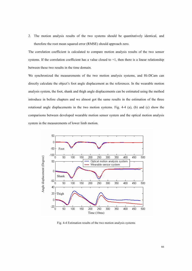
66

2. The motion analysis results of the two systems should be quantitatively identical, and

therefore the root mean squared error (RMSE) should approach zero.

The correlation coefficient is calculated to compare motion analysis results of the two sensor

systems. If the correlation coefficient has a value closed to +1, then there is a linear relationship

between these two results in the time domain.

We synchronized the measurements of the two motion analysis systems, and Hi-DCam can

directly calculate the object’s foot angle displacement as the references. In the wearable motion

analysis system, the foot, shank and thigh angle displacements can be estimated using the method

introduce in before chapters and we almost got the same results in the estimation of the three

rotational angle displacements in the two motion systems. Fig. 4-4 (a), (b) and (c) show the

comparisons between developed wearable motion sensor system and the optical motion analysis

system in the measurements of lower limb motion.

Fig. 4-4 Estimation results of the two motion analysis systems

Time (10ms)

Foot

Shank

Thigh

Ang

le d

ispl

acem

ent (

Deg

ree)

67

Chapter 5

Human Lower Limbs Dynamics Analysis

We are combining the developed wearable human motion analysis sensor system with the

reaction force sensor worn under foot to implement human dynamics analysis (Fig 5-1). The gait

phase division will improve the precision of this method by providing constrain condition about

the functional muscles for an optimum analysis. We have completed the analysis experiments on

ten subjects (average age: 21, average height 1.7m). The quantitative results of the sensor system

using direct integral calculation were compared with the measurements obtained with a

commercial optical motion analysis system and the referenced force plate.

68

Fig. 5-1 Wearable force and motion sensor system

5.1 Reaction Force Measurements The wearable force sensor system was attached to the bottom of the foot (Fig. 5-2). It can

measure three-direction forces and three-direction moments. Fig. 5-2 (b) defines the sensor

coordinate system XYZ that was used to express foot orientation and position relative to the

ground. The Y-axis was defined in the direction of progression, the Z-axis vertically and the

X-axis perpendicular to the Y- and Z-axes.

A set of experiments is finished on five subjects for system testing (four male subjects and one female

subject). At first, subject is asked to sit on a chair for about 3 seconds when the data sampling starts.

Multi-channel Data- recorder

Motion Senor Unit (Gyro)

Motion Senor Unit (Gyro and Ac)

Motion Senor Unit (Gyro)

Six-axis Force Sensor

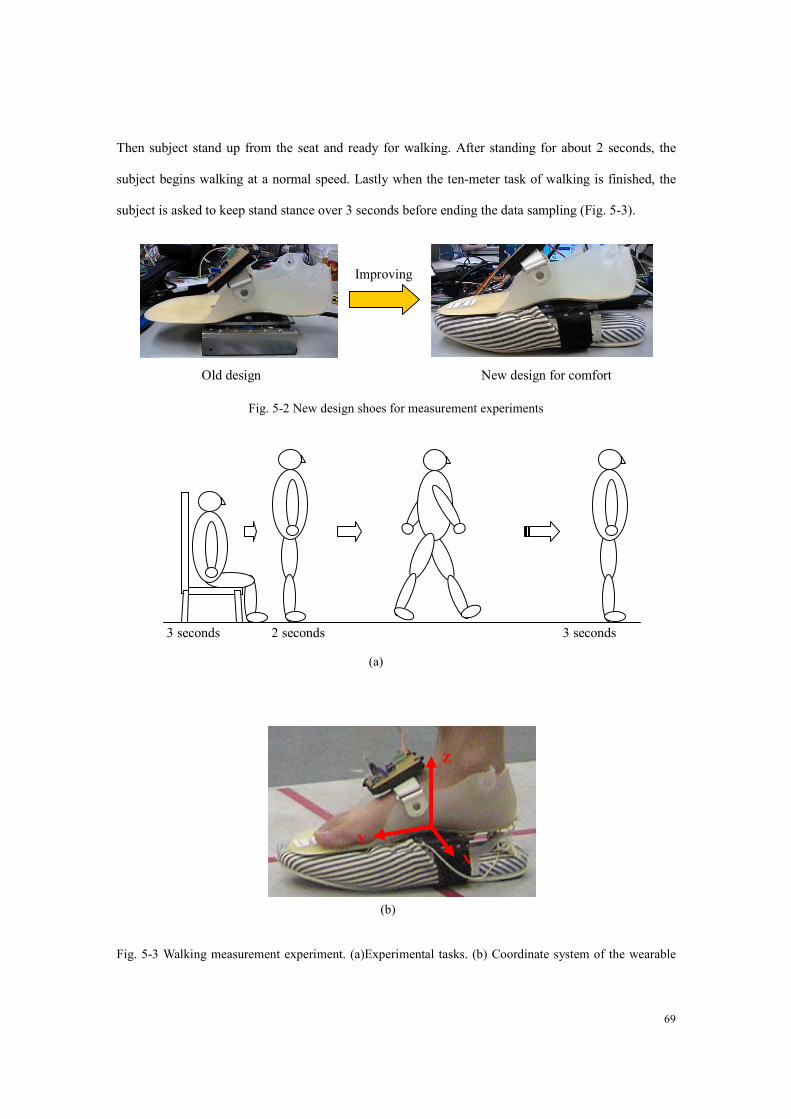
69

Then subject stand up from the seat and ready for walking. After standing for about 2 seconds, the

subject begins walking at a normal speed. Lastly when the ten-meter task of walking is finished, the

subject is asked to keep stand stance over 3 seconds before ending the data sampling (Fig. 5-3).

Fig. 5-2 New design shoes for measurement experiments

Fig. 5-3 Walking measurement experiment. (a)Experimental tasks. (b) Coordinate system of the wearable

(b)

Z

Y X

3 seconds 2 seconds 3 seconds

(a)

Old design New design for comfort

Improving

70

force sensor. The force sensor was taped to the shoe. The sensor signals were sampled using a portable data

recorder. The sensor coordinate system is indicated in Fig. b. The Y-axis coincides with the direction of

progression during walking, the Z-axis is directed vertically and the X-axis is defined perpendicular to Y-

and Z-axes. Positive X, Y, Z orientations are indicated.

When the human motion and force record were finished, the data in the data recorder would be

fed into personal computer through serial port (RS232), so walking data was prepared for the

offline motion analysis computing. The leg dynamics analysis was performed to estimate the leg

segments’ angular orientations and reaction forces.

71

Time (10 ms)

Thre

e-ax

is fo

rces

(Kgf

)

Sit-in Stance Walking

(a)

(b)

Y (mm) X (mm)

Forc

e ve

ctor

(10k

gf)

Stance

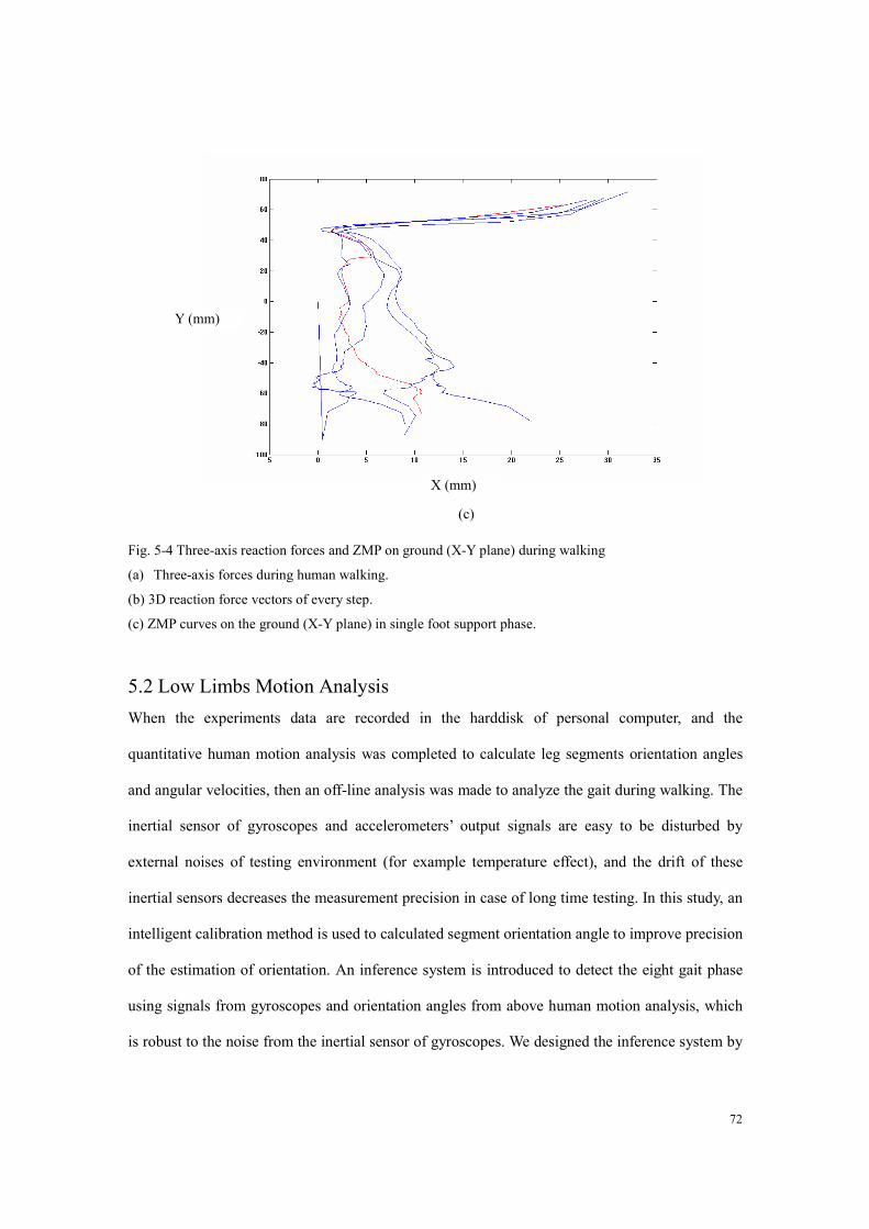
72

Fig. 5-4 Three-axis reaction forces and ZMP on ground (X-Y plane) during walking

(a) Three-axis forces during human walking.

(b) 3D reaction force vectors of every step.

(c) ZMP curves on the ground (X-Y plane) in single foot support phase.

5.2 Low Limbs Motion Analysis When the experiments data are recorded in the harddisk of personal computer, and the

quantitative human motion analysis was completed to calculate leg segments orientation angles

and angular velocities, then an off-line analysis was made to analyze the gait during walking. The

inertial sensor of gyroscopes and accelerometers’ output signals are easy to be disturbed by

external noises of testing environment (for example temperature effect), and the drift of these

inertial sensors decreases the measurement precision in case of long time testing. In this study, an

intelligent calibration method is used to calculated segment orientation angle to improve precision

of the estimation of orientation. An inference system is introduced to detect the eight gait phase

using signals from gyroscopes and orientation angles from above human motion analysis, which

is robust to the noise from the inertial sensor of gyroscopes. We designed the inference system by

X (mm)

Y (mm)

(c)

73

the aid of MATLAB software. The three gyroscopes’ signals and the three leg segments’

orientation angle were defined as six inputs vectors of this inference system. The inference rules

were designed from the algorithm of gait phase detection introduce in the second section. As

shown in Fig. 13, a human walking gait cycle is separated into eight phases according to this

inference system.

Fig. 5-5 Gait phase analysis-using results of the quantitative limb motion analysis. The three gyroscopes’

signals (angular velocities) and the three leg segments’ orientation angles were used to analyze a healthy

gait cycle which is divided into eight intervals of gait phases: initial contact, loading response, mid stance,

terminal stance, pre swing, initial swing, mid swing and terminal swing.

Initial contact

Load response

Mid

Early Late

Terminal stance

Pre-swing

Initial swing

Mid swing

Terminal swing

Orie

ntat

ion

angl

es (D

egre

e)

Ang

ular

vel

ociti

es (r

ad/s)

Time (ms)

74

Fig. 5-6 The lower limb motion analysis results based on the wearable motion sensor system.

5.3 Combination of the Developed Two Sensor System The experiment of the two wearable sensor systems for leg motion analysis was implemented in

the following three steps. Firstly, the sensor devices were worn on the subject’s leg to measure 2D

motion of leg (foot, shank and thigh) and six-axis reaction forces, and the sensors’ data were

saved in the pocketed data recorder. Secondly when the human motion and force record were

finished, the data in the data recorder would be fed into personal computer through serial port

75

(RS232), then walking data was prepared for the offline motion analysis computing. Finally, the

leg dynamics analysis was performed to estimate the leg segments’ angular orientations and

reaction forces.

We have completed the analysis experiments on ten subjects (average age: 21, average height

1.7m). To test drift error from the gyroscope worn on human body, we have compared the

quantitative results of the sensor system using direct integral calculation with the measurements

obtained with a commercial optical motion analysis system and the referenced force plate.

Fig. 5-7 Foot bottom reaction forces analysis and lower limb motion analysis results based on the wearable

sensor system.

Orie

ntat

ion

Ang

ular

(Deg

ree)

Th

ree-

axis

For

ce (k

gf)

Stance

Swing

Time (s)

76

Chapter 6

Conclusions

In this chapter, the entirety of the study project is considered. We begin with a summary of this

dissertation and the work to date. Comments on the short-term improvements to be made to the

current sensor systems and on the long-term potential of applications of these systems are given.

Overall, the work in this dissertation demonstrated that the developed sensor systems can be used

to acquire rich data about human motion and force, that we can devise efficient algorithms for

using this data in the detection of gait phases, and that the quantitative human motion analysis can

be implemented using the sensor systems. Further we show that a framework combining the force

sensor system and motion sensor system can be easily used to finish human dynamics analysis.

6.1 Summary The wearable sensor system we constructed uses a developed six-axis reaction force sensor to

measure ground reaction forces during human walking and uses some inertial measurement units

(gyroscope sensor and accelerometer) to collect data from the human motion of interest; data of

these sensors are saved in a developed data-recorder with a SRAM memory. After experiments

we import the sensor data into a personal computer through RS232 port, then the data are

analyzed with a designed algorithm to estimate lower limb angles and ground reaction forces, and

the generalized gait phase detection algorithms are applied to the human dynamics analysis, when

combines the reaction force analysis results form the wearable force sensor system. Each portion

of the wearable sensor system for human dynamics analysis is considered below.

We developed two prototypes of six-axis wearable force sensor with parallel mechanism to

77

measure ground-reaction forces in human dynamics analysis. A parallel flexible mechanism was

firstly designed for sensing impact forces and moments. Finite element method (FEM) was

conducted for dimension optimization. Sensitivity of the load cells in the force sensor was

improved by distributing strain gages on the maximum strain positions. A compact electrical

hardware system including amplifiers module, conditioning circuits and a microcomputer

controller was developed and integrated into the force sensor. The first prototype of a six-axis

force sensor was made to validate the theory of parallel-mechanism. The mass of the sensor is

about 300g, and its length, width and height are 170mm, 105mm and 26.5mm respectively. A new

parallel sensor was developed based on the No.1 sensor prototype for the future human dynamics

analysis. In order to make the mechanism more compact, hybrid measurement load cells were

adopted for X-and Y- direction translational forced measurement. The new design can decrease

the number of strain gauges and amplifier modules. The mass of the entire sensor system is about

0.5kg, and the whole dimensions are 115mm in length, 115mm in width and 35mm in height.

In this study, two inexpensive human motion analysis systems were constructed, in which

gyroscopes (ENC-05EB) were used to measure angular velocities of body segments, and two-axis

accelerometers (ADXL202) were used to measure the accelerations for the calibration in each

human motion cycle. The first wearable sensor system is designed for only foot motion analysis

and the second system can be used for a leg (foot, shank and thigh) motion analysis. Base on

the two sensor systems, a fuzzy inference system (FIS) is developed for the calculation of the gait

phases derived from sensors’ outputs. A digital filter is also designed to remove noises from of the

output of the fuzzy inference system, which enhances robustness of the system. Finally,

experimental study is conducted to validate the wearable sensor systems using an optical motion

analysis system.

At last, we combined the developed wearable human motion analysis sensor system with the

reaction force sensor worn under foot to implement human dynamics analysis. The gait phase

division improved the precision of this method by providing constrain condition about the

78

functional muscles for an optimum analysis. We have completed the analysis experiments on ten

subjects (average age: 21, average height 1.7m). The quantitative results of the sensor system

using direct integral calculation were compared with the measurements obtained with a

commercial optical motion analysis system and the referenced force plate.

6.2 Future Work As the intent of this dissertation work was to develop a wearable sensor system for human

dynamics analysis, there are a number of possible improvements to both the hardware and the

software that are worth noting. Further, there are fundamental design questions to be answered

regarding stand-alone devices, and they are discussed here as well.

The second prototype of the wearable reaction force is about 0.5kg, and the whole dimensions are

115mm in length, 115mm in width and 35mm in height (chapter 2). We find that this system is

still never comfortable enough for wearing applications, so a new reaction force sensor will be

developed with the same parallel flexible mechanism for sensing impact forces and moments.

Finite element method (FEM) will be used for dimension optimization in the new sensor design.

The next revision of the motion sensors hardware will be discussed for developing a 3D motion

analysis system using the inertial sensors (gyroscope and accelerometer), and three areas for

improvement will just be touched on here. Sensor size should be reduced, hopefully moving to

smaller accelerometers and MEMS gyroscopes in the near future. The device should also be more

flexible in shape, to allow for a greater range of applications. Finally, the precision of the motion

analysis system should be improved by using digital filter on chip.

In the human dynamics analysis stage, there is the possibility of combining the developed force

sensor system and the motion sensor system for estimating lower limb joint moment and muscle

tension using the results from force and motion analysis. As shown in Fig. 6-1, a muscle model is

proposed, and it should be possible to estimate leg muscle tensions from the results of human

lower limb motion and force analysis.

79

Fig. 6-1 Muscle tension estimation. By using the wearable force and motion sensor systems, we can

calculate leg joint moments (M1, M2 and M3), and then based on a muscle module of human leg, the main

muscle tension can be estimated.

6.3 Future Applications To comment on the future possibilities of the developed force and motion sensor system as not

just a human dynamics analysis device, but a controller interface for automation and robotics

applications and a health evaluation device for biomedical engineering applications [37]-[39], we

consider the somewhat whimsical example involving a wearable human motion analysis unit that

can be attached to any ordinary object.

We developed a small humanoid robot “R1” (height: 330mm and mass: 2kg) for the experimental

study. The word “data” is plural, not singular. In this robot, 12 sets of servo motor (Kondo

Kagaku Co., LTD) is used to make joints of two legs. As shown in Fig. 6-2, the human motion is

analyzed in real-time by using a personal computer, and the robot is controlled through a pair of

wireless module. A microcomputer controller (PIC 16F877A by Microchip Co) is inbuilt in the

robot, which can output the 12-channel pulses for the drive motors and connect with a wireless

M1 ankle joint

M2 knee joint

M3 hip joint

Muscle model

80

module. In this experiment, utilizing the analysis method introduced in the former sections of this

paper, we want to make the robot walk in the same phase as human walking.

Fig. 6-2 Humanoid robot control based on human motion analysis

This is just one possible example: other applications include health evaluation systems that make

balance evaluation in the health examination, and interfaces that can train patients in the exercise

of rehabilitation. Such systems would be beneficial to our everyday life.

PC

Human motion

Robot ( R1 )

81

References

[1] Gerald F. Harris, Peter A. Smith, “Human Motion Analysis,” Reading, IEEE, Inc., pp 12-30,

1996.

[2] Vladimir M. Zatsiorsky, “Kinetics of Human Motion,” Reading, Human kinetics Inc., 2001.

www.humankinetics.com.

[3] Roger M. Enoka, “Neuromechanics of Human Movement,” Reading, Human kinetics Inc.,

2001. www.humankinetics.com.

[4] Bonato, P. “Wearable sensors/systems and their impact on biomedical engineering,” IEEE

Eng. Med. Biol. Mag., 2003, 22 (3) pp. 18-20.

[5] Mehmet Engin, Alparslan Demirel, Erkan Zeki Engin, Musa Fedakar, “Recent developments

and trends in biomedical sensors,” Measurement, 2005,37, pp. 173-188

[6] Yoshio INOUE, Takuya MATSUDA, Kyoko SHIBATA, “Estimation of vertical reaction

force and ankle joint moment by using plantar pressure sensor,” JSME, Symposium on

human dynamics, pp.57-62, 2003. (In Japanese)

[7] Ledoux W.R, Hillstrom H.J, “The distributed plantar vertical force of neutrally aligned and

pes planus feet,” Gait and Posture, Vol.15, pp.1-9, 2002.

[8] Faivre A, Dahan M, Parratte B, Monnier G, “Instrumented shoes for pathological gait

assessment,” Mechanics Research Communications, Vol.31, pp.627-632, 2004.

[9] Lin Wang, David J Beebe, “Characterization of a silicon-based shear-force sensor on human

subjects,” IEEE Trans Biomed Eng, Vol.49, pp.1340-1347, 2002.

82

[10] Beccai L, Roccella S, Arena A, Valvo F, Valdastri P, Menciassi A, Carrozza M.C, Dario P,

“Design and fabrication of a hybrid silicon three-axial force sensor for biomechanical

applications,” Sensors and Actuators A: Physical, Vol.120, pp.370-382, 2005.

[11] Valdastri P, Roccella S, Beccai L, Cattin E, Menciassi A, Carrozza M.C, Dario P,

“Characterization of a novel hybrid silicon three-axial force sensor,” Sensors & Actuators: A.

Physical, Vol.123-124, pp.249-257, 2005.

[12] Chao L.-P, Yin C.-Y, “The six-component force sensor for measuring the loading of the feet

in locomotion,” Materials and Design, Vol.20, pp.237-244, 1999.

[13] Vazsonyi E, Adam M, Ducso Cs, Vizvary Z, Toth A.L, Barsony I, “Three-dimensional force

sensor by novel alkaline etching technique,” Sensors and Actuators: A. Physical, Vol.123-124,

pp.620-626, 2005.

[14] Sheng A Liu, “A novel six-component force sensor of good measurement isotropy and

sensitivities,” Sensor and Actuators, pp.223-230,2002.BN

[15] Koichi Nishiwaki, “A six-axis force sensor with parallel support mechanism to measure the

ground reaction force of humanoid robot,” Proceeding of the 2002 IEEE international

conference on robotics and automation, pp.2277-2282, 2002.

[16] Nolan L, Wit A, Dudzinski K, Lees A, Lake M, Wychowanski M, “Adjustments in gait

symmetry with walking speed in trans-femoral and trans-tibial amputees,” Gait and Posture,

pp.142-151, 2003.

[17] Aminian K, Trevisan C, Najafi B, Dejnabadi H, Frigo C, Pavan E, Telonio A, Robert P,

“Evaluation of an ambulatory system for gait analysis in hip osteoarthritis and after total hip

replacement,” Gait and Posture, Vol.20, pp.102-107, 2004.

[18] Kawakami H, Sugano N, Yonenobu K, Yoshikawa H, Ochi T, Hattori A, Suzuki N, “Gait

analysis system for assessment of dynamic loading axis of the knee,” Gait and Posture,

Vol.21, pp.125-130, 2005

83

[19] I.A. Karaulova, P.M. Hall, A.D. Marshall, “Tracking people in three dimensions using a

hierarchical model,” Image and Vision Computing, Vol.20, pp.691-700, 2002.

[20] Kim C.M, Eng J.J, “Magnitude and pattern of 3D kinematic and kinetic gait profiles in

persons with stroke: relationship to walking speed,” Gait and Posture, Vol.20, pp.140-146,

2004

[21] Casadio M, Morasso P.G, Sanguineti V, “Direct measurement of ankle stiffness during quiet

standing: implications for control modelling and clinical application,” Gait and Posture,

Vol.21, pp.410-424, 2005.

[22] Mathie M.J, Coster A.C.F, Lowell N.H, Celler B.G. “Accelerometry: Providing an integrated,

practical method for long-term, ambulatory monitoring of human movement,” Physiol.

Meas., 2004, 25 pp. 1-20.

[23] Aminian K, Rezakhanlou K, De Andres E, Fritsch C, Leyvraz P.F, Robert Ph. “Temporal

features estimation during walking using miniature accelerometers: An analysis of gait

improvement after hip arthroplasty,” Medical and Biological Engineering and Computation,

1999, 37 pp. 686-691.

[24] K. Tong and H. M. Granat, “A practical gait analysis system using gyroscopes,” Med. Eng.

Phys., 1999, vol. 21, pp. 87–94.

[25] Ion P. I. Pappas, Milos R. Popovic, Thierry Keller, Volker Dietz, and Manfred Morari, “A

reliable gait phase detection system,” IEEE Trans. Rehab. Eng., 2001, vol. 9, No. 2, pp.

113–125.

[26] R. Williamson and B. J. Andrews, “Gait event detection for FES using accelerometers and

supervised machine learning,” IEEE Trans. Rehab. Eng., 2000, vol. 8, pp. 312–319.

[27] Willemsen A.T, Bloemhof F, Boom H.B. “Automatic stance-swing phase detection from

accelerometer data for peroneal nerve stimulation,” IEEE Trans. Biomed. Eng.,1990, 37 pp.

1201-1208.

84

[28] H. J. Luinge, P. H. Veltink, “Measurement orientation of human body segments using

miniature gyroscopes and accelerometers,” Med. Biol. Eng. Comput., 2005, 43 pp. 273-282.

[29] Henk J. Luinge, Peter H. Veltink, “Inclination measurement of human movement using a

3-D accelerometer with autocalibration,” IEEE Trans. Rehab. Eng., 2004, 12 pp. 112-121.

[30] Giansanti D, Macellari V, Maccioni G, Cappozzo A. “Is it feasible to reconstruct body

segment 3-D position and orientation using accelerometric data?,” IEEE Trans. Biomed. Eng.,

2003, 50 pp. 476-483.

[31] Tao Liu, Yoshio Inoue, Kyoko Shibata, Yohei Yamasaki, Masafumi Nakahama, “A

Six-dimension Parallel Force Sensor for Human Dynamics Analysis,” Proceedings 2004

IEEE International Conference on Robotics, Automation and Mechatronics, Singapore,

pp. 208-212, 2004

[32] Tao Liu, Yoshio Inoue, Kyoko Shibata, Xueyan Tang, “A Wearable Inertial Sensor System

for Human Motion Analysis,” Proceedings 2005 IEEE International Symposium on

Computational Intelligence in Robotics and Automation, Finland, 2005, pp. 409-514

[33] Tao Liu, Yoshio Inoue, Kyoko Shibata, Haruhiko Morioka. “Development of Wearable

Sensor Combinations for Human Lower Extremity Motion Analysis” Proceedings of the 2006

IEEE International Conference on Robotics and Automation (ICRA2006), pp. 1655-1660.

[34] Pathokinesiology Department, Physical Therapy Department: “Observational Gait Analysis

Handbook.” CA, The professional staff association of rancho Los Amigos Medical Center,

1989.

[35] Jacquelin Parry. “Gait Analysis Normal and Pathological Function,” Slack Incorporated,

1992.

[36] John K. Taylor, Cheryl Cihon, “Statistical techniquws for data analysis,” Reading, A CRV

Press Company, 1996, pp206-209.

85

[37] Bouten C.V.C, Koekkoek K.T.M, Verduin M, Kodde R, Janssen J.D. “A triaxial

accelerometer and portable processing unit for the assessment of daily physical activity,”

IEEE Trans. Biomed. Eng., 1997, 44 pp. 136-147.

[38] Pedotti A., Krishnan V. V. and Stark L., “Optimization of muscle-force sequencing in human

locomotion,” Mathematical Biosciences, 38, pp. 57-76, 1978.

[39] Ehara Y., Beppu M., Nomura S., and Kunimi Y., “Estimation of energy consumption

during level walking,” Biomechanisms, (in Japanese), 10, pp. 163-172, 1990.

86

Appendix A

Abbreviations and Symbols

A/D Analog to digital converter.

DOF Degree of freedom.

FEA Finite element analysis

FEM Finite element method

FIS Fuzzy Inference System

MEMS Micro-electromechanical systems.

PCB Printed circuit board.

PE Percent Errors

RMS Root of the Mean of the Square differences

RS-232 Serial transmission protocol.

SRAM Static random access memory

ZMP Zero Moment Point

87

Appendix B Terminology in gait phase analysis 1. Initial contact: This phase includes the moment when the foot just touches the floor. The joint

postures presented at this time determine the limb’s loading response pattern.

2. Loading response: This is the initial double stance period. The phase begins with initial floor

contact and continues until the other foot is lifted for swing. Using the heel as a rocker, the knee

is flexed for shock absorption. Ankle plantar flexion limits the heel rocker by forefoot contact

with floor.

3. Mid stance: This is the first half of the single limb support interval. In this phase, the limb

advances over the stationary foot by ankle dorsiflexion (ankle rocker) while the knee and hip

extend. It begins as the other foot is lifted and continues until body weight is aligned over the

forefoot.

4. Terminal stance: This phase complete single limb support. It begins with heel rise and

continues until the other foot strikes the ground, in which the heel rise and the limb advance over

the forefoot rocker. Throughout his phase body weight moves ahead of the forefoot.

5. Pre-swing: This final phase of stance is the second double stance interval in the gait cycle. It

begins with initial contact of the opposite limb and end with ipsilateral toe-off. Objective of this

phase is position the limb for swing.

6. Initial swing: This phase is approximately one-third of the swing period. It begins with lift of

the foot from the floor and ends when the swinging foot is opposite the stance foot. In this phase,

the foot is lifted and limb advanced by hip flexion and increased knee flexion.

7. Mid swing: This phase begins as the swinging limb is opposite the stance limb and ends when

88

the swinging limb is forward and the tibia is vertical (i.e., hip and keen flexion postures are equal).

The knee is allowed to extend in response to gravity while the ankle continues dorsiflexion to

neural.

8. Terminal swing: This final phase of swing begins with a vertical tibia and ends when the foot

strikes the floor. Limb advancement is completed as the leg (shank) moves ahead of the thigh. In

this phase the limb advancement is completed by knee extension, and the hip maintains its earlier

flexion, and the ankle remains dorsiflexed to neural [16].

89

Appendix C Drawings, Schematics and PCB Layouts

90

Fig. C-1 Z- and Y- load cell drawing of No. 1 force sensor

91

Fig. C-2 X- load cell drawing of No. 1 force sensor

92

Fig. C-3 Blocks drawing of No. 1 force sensor

93

Fig. C-4 Bottom plane drawing of No. 1 force sensor

94

Fig. C-5 Top plane drawing of No. 1 force sensor

95

Fig. C-6 Bottom assemble drawing of No. 1 force sensor

96

Fig. C-7 Top assemble drawing of No. 1 force sensor

97

Fig. C-8 X- and Y- load cell drawing of No. 2 force sensor

98

Fig. C-9 Z- load cell drawing of No. 2 force sensor

99

Fig. C-10 Bottom plane drawing of No. 2 force sensor

100

Fig. C-11 Top plane drawing of No. 2 force sensor

101

Fig. C-12 Assemble drawing of No. 2 force sensor

102

Fig. C-13 Force sensor electrical board schematic

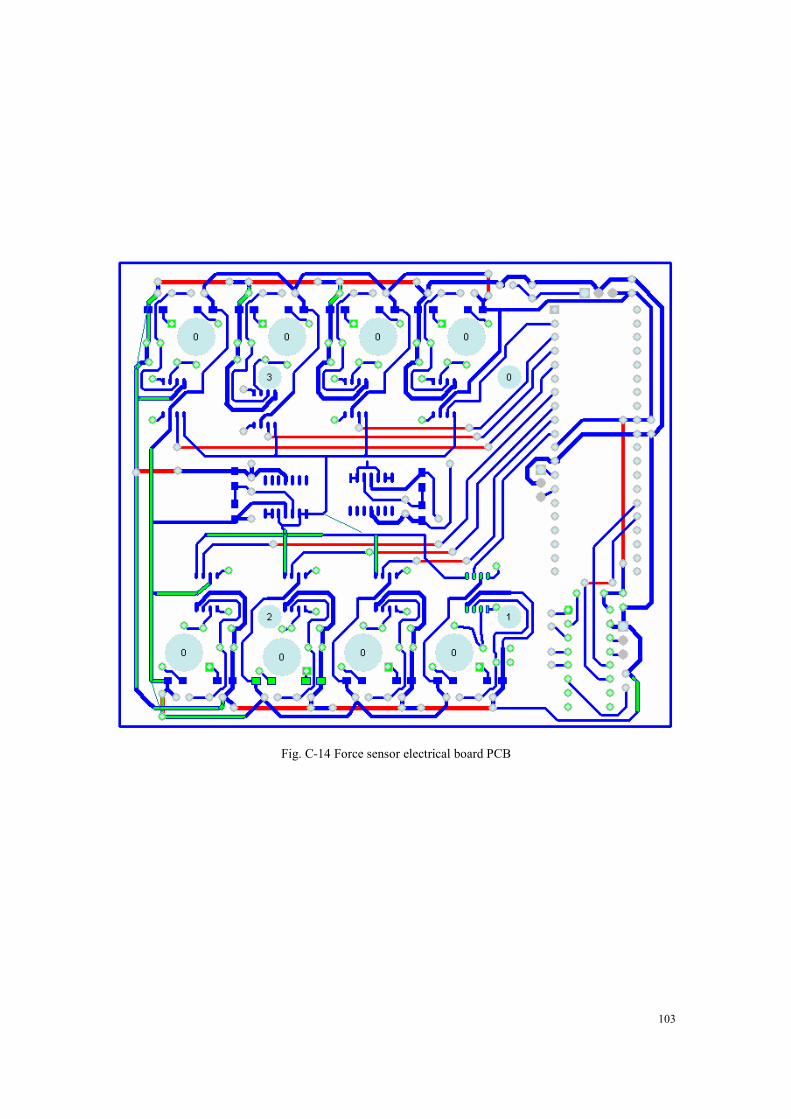
103

Fig. C-14 Force sensor electrical board PCB

104

Fig. C-15 No. 1 motion sensor electrical board schematic

105

Fig. C-16 No. 1 motion sensor electrical board PCB

106

Fig. C-17 No. 2 motion sensor electrical board (Sensor unit) schematic

107

Fig. C-18 No. 2 motion sensor electrical board (Sensor unit) PCB

108

Fig. C-19 No. 2 motion sensor electrical board (Accelerometer sensor) PCB

109

Fig. C-20 No. 2 motion sensor electrical board (Data recorder) schematic

110

Fig. C-21 No. 2 motion sensor electrical board (Data recorder) PCB

111

Appendix D

MATLAB Code (Offline analysis)

112

Acquiring Force and Motion Sensors Data

fp1=fopen('D:\Documents and Settings\liu\Desktop\My paper 2006\Experimental data\calibration\cal1.txt','r');% zheng693 %while(feof(fp1)==0) x=fscanf(fp1,'%x',[15,inf]); fp2=fopen('D:\Documents and Settings\liu\Desktop\My paper 2006\Experimental data\calibration\f1.txt','r');% zheng693 %while(feof(fp1)==0) y=fscanf(fp2,'%f',[9,inf]); %x=x(:,680:1984); y=y'; fx=y(:,2); fy=y(:,3); fz=y(:,4); Ch1=x(1,:)'; Ch2=x(2,:)'; Ch3=x(3,:)'; Ch4=x(4,:)'; Ch5=x(5,:)'; Ch6=x(6,:)'; Ch7=x(7,:)'; Ch8=x(8,:)'; Ch9=x(9,:)'; Ch10=x(10,:)'; Ch11=x(11,:)'; Ch12=x(12,:)'; Ch13=x(13,:)'; zCh1=sum(Ch1(1:20))/20; zCh2=sum(Ch2(1:20))/20; zCh3=sum(Ch3(1:20))/20; zCh4=sum(Ch4(1:20))/20; zCh5=sum(Ch5(1:20))/20; zCh6=sum(Ch6(1:20))/20; zCh7=sum(Ch7(1:20))/20; zCh8=sum(Ch8(1:20))/20; zCh9=sum(Ch9(1:20))/20; zCh10=sum(Ch10(1:20))/20; zCh11=sum(Ch11(1:20))/20; zCh12=sum(Ch12(1:20))/20; zCh13=sum(Ch13(1:20))/20; RCh1=(Ch1-526.1)*5/1023; RCh2=(Ch2-496)*5/1023;

RCh3=(Ch3-499.5)*5/1023; RCh4=(Ch4-499.35)*5/1023; RCh5=(Ch5-497.7)*5/1023; RCh6=(Ch6-502.9)*5/1023; RCh7=(Ch7-500.6)*5/1023; RCh8=(Ch8-502.7)*5/1023; RCh9=(Ch9-zCh9)*5/1023; RCh10=(Ch10-zCh10)*5/1023; RCh11=(Ch11-zCh11)*5/1023; RCh12=(Ch12-zCh12)*5/1023; RCh13=(Ch13-zCh13)*5/1023; Fz=RCh1*25.056+RCh4*21.693+RCh5*24.899+RCh8*27.572; Fx=-RCh3*230.756+RCh7*255.255; Fy=RCh2*256.1+RCh6*249.406;%RCh2*397.6+RCh6*233.5 figure(1) subplot(3,1,1) plot(Fz(442:1000)) hold; plot(fz(475:1000)/10,'r') legend('Fz','fx'); subplot(3,1,2) plot(Fx(442:1000)/10) hold; plot(fx(475:1000)/10,'r') legend('Fx','fx');

subplot(3,1,3)

plot(Fy(442:1000)/10)

hold;

plot(fy(475:1000)/10,'r')

legend('Fy','fy');

113

Fr=evalfis(Fuzzyinput, Gait1); Fro=Fr; lenF=size(Fr); %filter (1 point filter) for i=2:(lenF(1)-1) if (abs(Fr(i-1)-Fr(i+1))<0.1)&(abs(Fr(i-1)-Fr(i))>1) Fr(i)=Fr(i-1); end end %filter (2 point filter) for i=2:(lenF(1)-2) if (abs(Fr(i-1)-Fr(i+2))<0.1)&(abs(Fr(i+1)-Fr(i))<0.1)&(abs(Fr(i)-Fr(i+2))>1) Fr(i)=Fr(i-1); Fr(i+1)=Fr(i-1); end end %filter (3 point filter) for i=2:(lenF(1)-3) if (abs(Fr(i-1)-Fr(i+3))<0.1)&(abs(Fr(i+1)-Fr(i))<0.1)&(abs(Fr(i+1)-Fr(i+2))<0.1)&(abs(Fr(i)-Fr(i+3))>1) Fr(i)=Fr(i-1); Fr(i+1)=Fr(i-1); Fr(i+2)=Fr(i-1); end end %filter (4 point filter) for i=2:(lenF(1)-4) if (abs(Fr(i-1)-Fr(i+4))<0.1)&(abs(Fr(i+1)-Fr(i))<0.1)&(abs(Fr(i+1)-Fr(i+2))<0.1)&(abs(Fr(i+2)-Fr(i+3))<0.1)&(abs(Fr(i)-Fr(i+4))>1) Fr(i)=Fr(i-1); Fr(i)=Fr(i-1); Fr(i+1)=Fr(i-1); Fr(i+2)=Fr(i-1); Fr(i+3)=Fr(i-1); end end %filter (5 point filter) for i=2:(lenF(1)-5) if (abs(Fr(i-1)-Fr(i+5))<0.1)&(abs(Fr(i+1)-Fr(i))<0.1)&(abs(Fr(i+1)-Fr(i+2))<0.1)&(abs(Fr(i+2)-Fr(i+3))<0.1)&(abs(Fr(i+3)-Fr(i+4))<0.1)&(abs(Fr(i)-Fr(i+5))>2) Fr(i)=Fr(i-1); Fr(i)=Fr(i-1); Fr(i)=Fr(i-1); Fr(i+1)=Fr(i-1); Fr(i+2)=Fr(i-1); Fr(i+3)=Fr(i-1); Fr(i+4)=Fr(i-1);

114

end end %filter (6 point filter) for i=2:(lenF(1)-6) if (abs(Fr(i-1)-Fr(i+6))<0.1)&(abs(Fr(i+1)-Fr(i))<0.1)&(abs(Fr(i+1)-Fr(i+2))<0.1)&(abs(Fr(i+2)-Fr(i+3))<0.1)&(abs(Fr(i+3)-Fr(i+4))<0.1)&(abs(Fr(i+4)-Fr(i+5))<0.1)&(abs(Fr(i)-Fr(i+6))>2) Fr(i)=Fr(i-1); end end j=1; k=1; for i=5:(lenF(1)-6) if ((abs(Fr(i-4)-Fr(i-3))<0.1)&(abs(Fr(i-3)-Fr(i-2))<0.1)&(abs(Fr(i-2)-Fr(i-1))<0.1)&(abs(Fr(i-1)-Fr(i))<0.1)&(abs(Fr(i-1)-Fr(i))<0.1)&((Fr(i+1)-Fr(i))>4)&(abs(Fr(i+1)-Fr(i+2))<0.1)&(abs(Fr(i+2)-Fr(i+3))<0.1)&(abs(Fr(i+3)-Fr(i+4))<0.1)&(abs(Fr(i+4)-Fr(i+5))<0.1)&(abs(Fr(i+5)-Fr(i+6))<0.1)) Fp(j,k)=i; k=k+1; elseif (abs(Fr(i-4)-Fr(i-3))<0.1)&(abs(Fr(i-3)-Fr(i-2))<0.1)&(abs(Fr(i-2)-Fr(i-1))<0.1)&(abs(Fr(i-1)-Fr(i))<0.1)&((Fr(i+1)-Fr(i))>1)&((Fr(i+1)-Fr(i))<4)&(abs(Fr(i+1)-Fr(i+2))<0.1)&(abs(Fr(i+2)-Fr(i+3))<0.1)&(abs(Fr(i+3)-Fr(i+4))<0.1)&(abs(Fr(i+4)-Fr(i+5))<0.1)&(abs(Fr(i+5)-Fr(i+6))<0.1) Fp(j,k)=i; k=k+1; elseif (abs(Fr(i-4)-Fr(i-3))<0.1)&(abs(Fr(i-3)-Fr(i-2))<0.1)&(abs(Fr(i-2)-Fr(i-1))<0.1)&(abs(Fr(i-1)-Fr(i))<0.1)&((Fr(i)-Fr(i+1))>1)&((Fr(i)-Fr(i+1))<4)&(abs(Fr(i+1)-Fr(i+2))<0.1)&(abs(Fr(i+2)-Fr(i+3))<0.1)&(abs(Fr(i+3)-Fr(i+4))<0.1)&(abs(Fr(i+4)-Fr(i+5))<0.1)&(abs(Fr(i+5)-Fr(i+6))<0.1) Fp(j,k)=i; k=k+1; elseif (abs(Fr(i-4)-Fr(i-3))<0.1)&(abs(Fr(i-3)-Fr(i-2))<0.1)&(abs(Fr(i-2)-Fr(i-1))<0.1)&(abs(Fr(i-1)-Fr(i))<0.1)&((Fr(i)-Fr(i+1))>4)&(abs(Fr(i+1)-Fr(i+2))<0.1)&(abs(Fr(i+2)-Fr(i+3))<0.1)&(abs(Fr(i+3)-Fr(i+4))<0.1)&(abs(Fr(i+4)-Fr(i+5))<0.1)&(abs(Fr(i+5)-Fr(i+6))<0.1) Fp(j,k)=i; k=1; j=j+1; end end

115

lenfp=size(Fp); j=1; for i=1:(lenF(1)) if i>Fp(j,1) & i<=Fp(j,2) FrN(i)=6; elseif i>Fp(j,2) & i<=Fp(j,3) FrN(i)=7.5; elseif i>Fp(j,3) & i<Fp(j,4) FrN(i)=10; elseif i==Fp(j,4) FrN(i)=10; j=j+1; if j>=lenfp(1,1)+1 j=lenfp(1,1); end else FrN(i)=1.5; end end end for j=1:lenfp(1,1) AxR(Fp(j,1):Fp(j,2))=AxR(Fp(j,1):Fp(j,2))-0.15*gyR(Fp(j,1):Fp(j,2)).*gyR(Fp(j,1):Fp(j,2)); AxR(Fp(j,3):Fp(j,4))=AxR(Fp(j,3):Fp(j,4))+0.1*gyR(Fp(j,3):Fp(j,4)).*gyR(Fp(j,3):Fp(j,4)); end

116

Acknowledgments To my advisor Prof. Yoshio Inoue, who provided me with his enthusiastic suggestions and advice

to support my research works. If I am one day a nice researcher, much of it will be his doing.

To my vice-advisor Prof. Kyoko Shibata, who gave me so many useful suggestions and

information about the project in every discussion meeting.

To my tutor Mr. Nakano, Matsumura, Kimura, my good friends, who helped me so much on

Japanese study and foreign life when I just went to Japan. I will never forget their warm heart and

kindness.

To Nakahama, an experienced researcher, his willing suggestion and good experience on

mechanical and electronic field help me so much.

To all the other members of Robotics and Dynamic Lab, make me feel so fine and happy. Special

acknowledgments to Chen chaochao and Zheng rencheng who brought me so many helps and

smiles.

At last but no least, thank SSP of KUT and Kokuhi Scholarship of Japanese Government

(Monbukagaku-sho) for kind supports.