9A.2 DETERMINATION OF THERMAL ROUGHNESS LENGTH FOR BUILT ENVIRONMENT WITH HIGH RESOLUTION WIRELESS METEOROLOGICAL STATIONS

Daniel F. Nadeau*, E. Bou-Zeid, M. B. Parlange, G. Barrenetxea, and M. Vetterli

École Polytechnique Fédérale de Lausanne, Switzerland

1. INTRODUCTION

Today, most of the worldwide population live and work in urban areas. As the urbanization process is expected to increase in the coming years, the need to better understand the impacts of man-made structures on the environment, and more particularly on the lower atmosphere, appears more than necessary.

The Monin-Obukhov similarity theory (MOST) remains the most commonly used tool to study land-atmosphere interactions in the atmospheric boundary layer. Although MOST is valid in the surface layer located over flat and homogeneous terrain (Beljaars and Holtslag, 1991), previous studies have used it over heterogeneous terrain (Brutsaert, 1998; Bou-Zeid et al, 2007). However, whether it applies or not for complex urban settings needs to be investigated.

A first step in urban canopies studies is typically to characterize the surface roughness. Higher roughness will increase turbulence production and thus will lead to enhanced mixing. This will in turn impact on the dynamics of surface fluxes and other land-atmosphere interactions.

When it comes down to finding roughness parameters for MOST, two approaches exist: the morphometric method and the micrometeorological method. The morphometric approach computes the roughness parameters based on the geometry of the urban canopy (building height, spacing, etc.), whereas micrometeorological approaches make use of in situ atmospheric profiles in the surface layer. Several morphometric models have been developed, however the dependency of the momentum surface roughness on the wind direction is rarely accounted for. In addition, the different models often lead to widely varying estimates of roughness characteristics and no comprehensive study was able to compare these models to robust micrometeorological measurements and assess their accuracy (Grimmond and Oke, 1999). For this reason, we focus here on the use of micrometeorological measurements to determine surface roughness.                                                             * Corresponding author address: Daniel F. Nadeau, EPFL, ISTE, 1015 – Lausanne, Switzerland, +41.21.693.8093; e-mail: daniel.nadeau@epfl.ch

This short paper will focus on the surface roughness determination as a first step toward the study of thermal roughness length in built environments. The following questions regarding the surface roughness in complex urban areas will thus be studied: what is the dependency of the surface roughness on the zero-displacement height and on the time of the day when the measurement was made? How does the surface roughness vary with wind direction?

2. BACKGROUND

Under neutral conditions, there is strong mechanical mixing and the turbulence is not affected by buoyancy effects. MOST for wind velocity profiles thus reduces to:

0*

0ln⎛ ⎞−

= ⎜ ⎟⎜ ⎟⎝ ⎠

z duuk z

(1)

where u is the wind speed at height z above the surface, u* is the friction velocity, k is the Von Karman’s constant and z0 is the aerodynamic roughness length (all in SI units). For very rough surfaces, where the height of the roughness elements is not negligible compared to the measurements height, it is necessary to introduce a zero- displacement height d0 (Brutsaert, 1982).

When no direct measurements of friction velocity or heat fluxes are available, a good way to assess the stability of atmospheric profiles is the gradient Richardson number Rig:

2 2

v

vg

gzRi

U Vz z

θθ

∂∂=

⎡ ⎤⎛ ⎞ ⎛ ⎞∂ ∂⎢ ⎥+⎜ ⎟ ⎜ ⎟⎜ ⎟ ⎜ ⎟⎢ ⎥∂ ∂⎝ ⎠ ⎝ ⎠⎣ ⎦

(2)

where g is the acceleration due to gravity, θv is the virtual potential temperature, U and V are the eastward and northward components of the wind velocity, respectively.

3. METHODS

The site of interest is the campus of the École Polytechnique Fédérale de Lausanne (see Figure 1), a

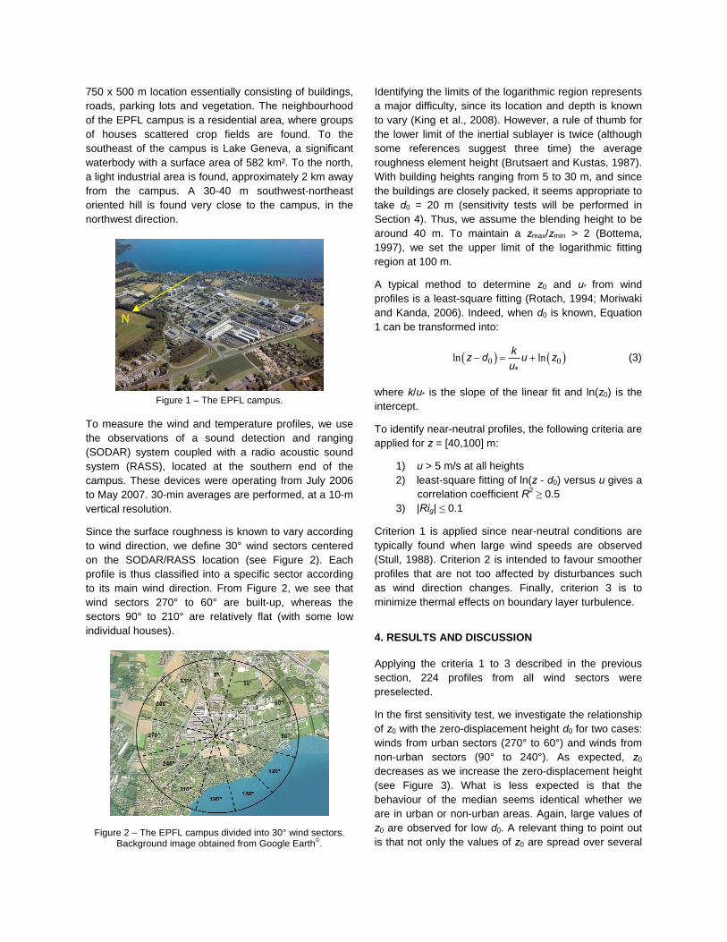
750 x 500 m location essentially consisting of buildings, roads, parking lots and vegetation. The neighbourhood of the EPFL campus is a residential area, where groups of houses scattered crop fields are found. To the southeast of the campus is Lake Geneva, a significant waterbody with a surface area of 582 km². To the north, a light industrial area is found, approximately 2 km away from the campus. A 30-40 m southwest-northeast oriented hill is found very close to the campus, in the northwest direction.

Figure 1 – The EPFL campus.

To measure the wind and temperature profiles, we use the observations of a sound detection and ranging (SODAR) system coupled with a radio acoustic sound system (RASS), located at the southern end of the campus. These devices were operating from July 2006 to May 2007. 30-min averages are performed, at a 10-m vertical resolution.

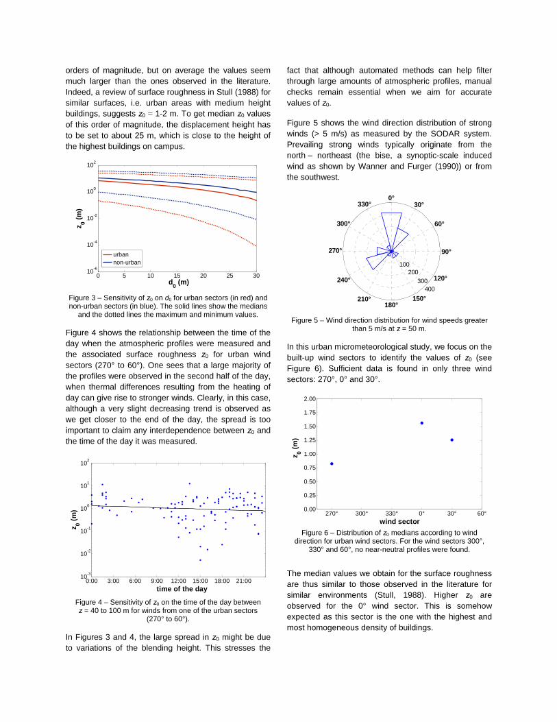
Since the surface roughness is known to vary according to wind direction, we define 30° wind sectors centered on the SODAR/RASS location (see Figure 2). Each profile is thus classified into a specific sector according to its main wind direction. From Figure 2, we see that wind sectors 270° to 60° are built-up, whereas the sectors 90° to 210° are relatively flat (with some low individual houses).

Figure 2 – The EPFL campus divided into 30° wind sectors. Background image obtained from Google Earth©.

Identifying the limits of the logarithmic region represents a major difficulty, since its location and depth is known to vary (King et al., 2008). However, a rule of thumb for the lower limit of the inertial sublayer is twice (although some references suggest three time) the average roughness element height (Brutsaert and Kustas, 1987). With building heights ranging from 5 to 30 m, and since the buildings are closely packed, it seems appropriate to take d0 = 20 m (sensitivity tests will be performed in Section 4). Thus, we assume the blending height to be around 40 m. To maintain a zmax/zmin > 2 (Bottema, 1997), we set the upper limit of the logarithmic fitting region at 100 m.

A typical method to determine z0 and u* from wind profiles is a least-square fitting (Rotach, 1994; Moriwaki and Kanda, 2006). Indeed, when d0 is known, Equation 1 can be transformed into:

( ) ( )0 0*

ln lnkz d u zu

− = + (3)

where k/u* is the slope of the linear fit and ln(z0) is the intercept.

To identify near-neutral profiles, the following criteria are applied for z = [40,100] m:

1) u > 5 m/s at all heights 2) least-square fitting of ln(z - d0) versus u gives a

correlation coefficient R2 ≥ 0.5 3) |Rig| ≤ 0.1

Criterion 1 is applied since near-neutral conditions are typically found when large wind speeds are observed (Stull, 1988). Criterion 2 is intended to favour smoother profiles that are not too affected by disturbances such as wind direction changes. Finally, criterion 3 is to minimize thermal effects on boundary layer turbulence. 4. RESULTS AND DISCUSSION

Applying the criteria 1 to 3 described in the previous section, 224 profiles from all wind sectors were preselected.

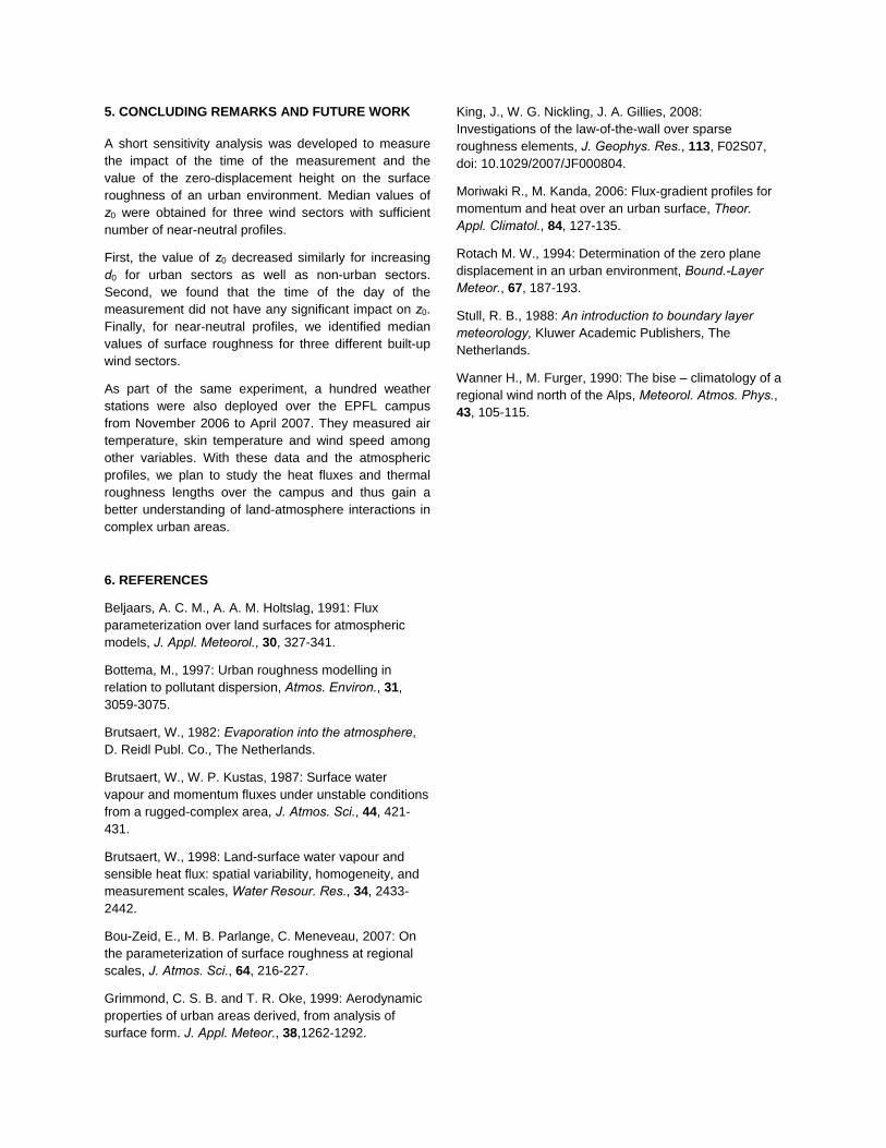
In the first sensitivity test, we investigate the relationship of z0 with the zero-displacement height d0 for two cases: winds from urban sectors (270° to 60°) and winds from non-urban sectors (90° to 240°). As expected, z0 decreases as we increase the zero-displacement height (see Figure 3). What is less expected is that the behaviour of the median seems identical whether we are in urban or non-urban areas. Again, large values of z0 are observed for low d0. A relevant thing to point out is that not only the values of z0 are spread over several

N 

orders of magnitude, but on average the values seem much larger than the ones observed in the literature. Indeed, a review of surface roughness in Stull (1988) for similar surfaces, i.e. urban areas with medium height buildings, suggests z0 ≈ 1-2 m. To get median z0 values of this order of magnitude, the displacement height has to be set to about 25 m, which is close to the height of the highest buildings on campus.

0 5 10 15 20 25 3010-6

10-4

10-2

100

102

d0 (m)

z 0 (m)

urbannon-urban

Figure 3 – Sensitivity of z0 on d0 for urban sectors (in red) and non-urban sectors (in blue). The solid lines show the medians

and the dotted lines the maximum and minimum values.

Figure 4 shows the relationship between the time of the day when the atmospheric profiles were measured and the associated surface roughness z0 for urban wind sectors (270° to 60°). One sees that a large majority of the profiles were observed in the second half of the day, when thermal differences resulting from the heating of day can give rise to stronger winds. Clearly, in this case, although a very slight decreasing trend is observed as we get closer to the end of the day, the spread is too important to claim any interdependence between z0 and the time of the day it was measured.

0:00 3:00 6:00 9:00 12:00 15:00 18:00 21:0010-3

10-2

10-1

100

101

102

time of the day

z 0 (m)

Figure 4 – Sensitivity of z0 on the time of the day between z = 40 to 100 m for winds from one of the urban sectors

(270° to 60°).

In Figures 3 and 4, the large spread in z0 might be due to variations of the blending height. This stresses the

fact that although automated methods can help filter through large amounts of atmospheric profiles, manual checks remain essential when we aim for accurate values of z0.

Figure 5 shows the wind direction distribution of strong winds (> 5 m/s) as measured by the SODAR system. Prevailing strong winds typically originate from the north – northeast (the bise, a synoptic-scale induced wind as shown by Wanner and Furger (1990)) or from the southwest.

100 200

300 400

60°

240°

30°

210°

0°

180°

330°

150°

300°

120°

270° 90°

Figure 5 – Wind direction distribution for wind speeds greater

than 5 m/s at z = 50 m.

In this urban micrometeorological study, we focus on the built-up wind sectors to identify the values of z0 (see Figure 6). Sufficient data is found in only three wind sectors: 270°, 0° and 30°.

270° 300° 330° 0° 30° 60°0.00

0.25

0.50

0.75

1.00

1.25

1.50

1.75

2.00

wind sector

z 0 (m)

Figure 6 – Distribution of z0 medians according to wind

direction for urban wind sectors. For the wind sectors 300°, 330° and 60°, no near-neutral profiles were found.

The median values we obtain for the surface roughness are thus similar to those observed in the literature for similar environments (Stull, 1988). Higher z0 are observed for the 0° wind sector. This is somehow expected as this sector is the one with the highest and most homogeneous density of buildings.

5. CONCLUDING REMARKS AND FUTURE WORK

A short sensitivity analysis was developed to measure the impact of the time of the measurement and the value of the zero-displacement height on the surface roughness of an urban environment. Median values of z0 were obtained for three wind sectors with sufficient number of near-neutral profiles.

First, the value of z0 decreased similarly for increasing d0 for urban sectors as well as non-urban sectors. Second, we found that the time of the day of the measurement did not have any significant impact on z0. Finally, for near-neutral profiles, we identified median values of surface roughness for three different built-up wind sectors.

As part of the same experiment, a hundred weather stations were also deployed over the EPFL campus from November 2006 to April 2007. They measured air temperature, skin temperature and wind speed among other variables. With these data and the atmospheric profiles, we plan to study the heat fluxes and thermal roughness lengths over the campus and thus gain a better understanding of land-atmosphere interactions in complex urban areas.

6. REFERENCES

Beljaars, A. C. M., A. A. M. Holtslag, 1991: Flux parameterization over land surfaces for atmospheric models, J. Appl. Meteorol., 30, 327-341.

Bottema, M., 1997: Urban roughness modelling in relation to pollutant dispersion, Atmos. Environ., 31, 3059-3075.

Brutsaert, W., 1982: Evaporation into the atmosphere, D. Reidl Publ. Co., The Netherlands.

Brutsaert, W., W. P. Kustas, 1987: Surface water vapour and momentum fluxes under unstable conditions from a rugged-complex area, J. Atmos. Sci., 44, 421-431.

Brutsaert, W., 1998: Land-surface water vapour and sensible heat flux: spatial variability, homogeneity, and measurement scales, Water Resour. Res., 34, 2433-2442.

Bou-Zeid, E., M. B. Parlange, C. Meneveau, 2007: On the parameterization of surface roughness at regional scales, J. Atmos. Sci., 64, 216-227.

Grimmond, C. S. B. and T. R. Oke, 1999: Aerodynamic properties of urban areas derived, from analysis of surface form. J. Appl. Meteor., 38,1262-1292.

King, J., W. G. Nickling, J. A. Gillies, 2008: Investigations of the law-of-the-wall over sparse roughness elements, J. Geophys. Res., 113, F02S07, doi: 10.1029/2007/JF000804.

Moriwaki R., M. Kanda, 2006: Flux-gradient profiles for momentum and heat over an urban surface, Theor. Appl. Climatol., 84, 127-135.

Rotach M. W., 1994: Determination of the zero plane displacement in an urban environment, Bound.-Layer Meteor., 67, 187-193.

Stull, R. B., 1988: An introduction to boundary layer meteorology, Kluwer Academic Publishers, The Netherlands.

Wanner H., M. Furger, 1990: The bise – climatology of a regional wind north of the Alps, Meteorol. Atmos. Phys., 43, 105-115.