A 439819

NAVAL POSTGRADUATE

SCHOOL

MONTEREY, CALIFORNIA

THESIS

Approved for public release; distribution is unlimited

MODELING, SIMULATION AND PERFORMANCE ANALYSIS OF MULTIPLE-INPUT MULTIPLE-OUTPUT

(MIMO) SYSTEMS WITH MULTICARRIER TIME DELAY DIVERSITY MODULATION

by

Muhammad Shahid

September 2005

Thesis Advisor: Frank Kragh Second Reader: Tri Ha

THIS PAGE INTENTIONALLY LEFT BLANK

i

REPORT DOCUMENTATION PAGE Form Approved OMB No. 0704-0188 Public reporting burden for this collection of information is estimated to average 1 hour per response, including the time for reviewing instruction, searching existing data sources, gathering and maintaining the data needed, and completing and reviewing the collection of information. Send comments regarding this burden estimate or any other aspect of this collection of information, including suggestions for reducing this burden, to Washington headquarters Services, Directorate for Information Operations and Reports, 1215 Jefferson Davis Highway, Suite 1204, Arlington, VA 22202-4302, and to the Office of Management and Budget, Paperwork Reduction Project (0704-0188) Washington DC 20503. 1. AGENCY USE ONLY (Leave blank)

2. REPORT DATE September 2005

1. AGENCY USE ONLY (Leave blank)

4. TITLE AND SUBTITLE: Modeling, Simulation and Performance Analysis of Multiple-Input Multiple-Output (MIMO) Systems with Multicarrier Time Delay Diversity Modulation 6. AUTHOR(S) Muhammad Shahid

5. FUNDING NUMBERS

7. PERFORMING ORGANIZATION NAME(S) AND ADDRESS(ES) Naval Postgraduate School Monterey, CA 93943-5000

8. PERFORMING ORGANIZATION REPORT NUMBER

9. SPONSORING /MONITORING AGENCY NAME(S) AND ADDRESS(ES) N/A

10. SPONSORING/MONITORING AGENCY REPORT NUMBER

11. SUPPLEMENTARY NOTES The views expressed in this thesis are those of the author and do not reflect the official policy or position of the Department of Defense or the U.S. Government. 12a. DISTRIBUTION / AVAILABILITY STATEMENT Approved for public release; distribution is unlimited

12b. DISTRIBUTION CODE

13. ABSTRACT (maximum 200 words) This thesis investigates the fundamentals of multiple-input single-output (MISO) and multiple-input

multiple-output (MIMO) radio communication systems with space-time codes. A MISO system and MIMO systems were designed using multicarrier delay diversity modulation (MDDM). MDDM was incorporated with orthogonal frequency division multiplexing (OFDM). The design was implemented with binary phase shift keying (BPSK). Matlab was used to simulate the design, which was tested in both an additive white Gaussian noise (AWGN) channel and in a slow fading frequency nonselective multipath channel with AWGN. The receiver design was incorporated with the maximal ratio combiner (MRC) receiving technique with perfect knowledge of channel state information (CSI). The theoretical performance was derived for both channels and was compared with the simulated results.

15. NUMBER OF PAGES

119

14. SUBJECT TERMS Multiple-input Single-output (MISO), Multiple-input Multiple-output (MIMO), Orthogonal Frequency Division Multiplexing (OFDM), Binary Phase Shift Keying, Rayleigh Fading Channel, Maximal Ratio Combining (MRC), Spatial Diversity

16. PRICE CODE 17. SECURITY CLASSIFICATION OF REPORT

Unclassified

18. SECURITY CLASSIFICATION OF THIS PAGE

Unclassified

17. SECURITY CLASSIFICATION OF REPORT

Unclassified

18. SECURITY CLASSIFICATION OF THIS PAGE

UL NSN 7540-01-280-5500 Standard Form 298 (Rev. 2-89) Prescribed by ANSI Std. 239-18

ii


iii

Approved for public release; distribution is unlimited

MODELING, SIMULATION AND PERFORMANCE ANALYSIS OF MULTIPLE-INPUT MULTIPLE-OUTPUT (MIMO) SYSTEMS WITH

MULTICARRIER DELAY DIVERSITY MODULATION (MDDM)

Muhammad Shahid Squadron Leader, Pakistan Air Force

B.S., NED University Karachi, Pakistan, 1993

Submitted in partial fulfillment of the requirements for the degree of

MASTER OF SCIENCE IN ELECTRICAL ENGINEERING

from the

NAVAL POSTGRADUATE SCHOOL September 2005

Author: Muhammad Shahid

Approved by: Frank Kragh

Thesis Advisor

Tri Ha Second Reader

Jeffrey B. Knorr Chairman, Department of Electrical and Computer Engineering

iv


v

ABSTRACT

This thesis investigates the fundamentals of multiple-input single-output (MISO)

and multiple-input multiple-output (MIMO) radio communication systems with space-

time codes. A MISO system and MIMO systems were designed using multicarrier delay

diversity modulation (MDDM). MDDM was incorporated with orthogonal frequency

division multiplexing (OFDM). The design was implemented with binary phase shift

keying (BPSK). Matlab was used to simulate the design, which was tested in both an

additive white Gaussian noise (AWGN) channel and in a slow fading frequency

nonselective multipath channel with AWGN. The receiver design was incorporated with

the maximal ratio combiner (MRC) receiving technique with perfect knowledge of

channel state information (CSI). The theoretical performance was derived for both

channels and was compared with the simulated results.

vi


vii

TABLE OF CONTENTS

I. INTRODUCTION........................................................................................................1 A. BACKGROUND ..............................................................................................1 B. OBJECTIVE AND METHODOLOGY.........................................................2 C. RELATED RESEARCH.................................................................................2 D. THESIS ORGANIZATION............................................................................2

II. MIMO SYSTEMS AND MULTICARRIER DELAY DIVERSITY ......................5 A. MULTIPLE-INPUT MULTIPLE-OUTPUT (MIMO) SYSTEMS.............5

1. Single-Input Single-Output System....................................................5 2. Single-Input Multiple-Output System................................................6 3. Multiple-Input Single-Output System................................................7 4. Multiple-Input Multiple-Output System ...........................................8

B. SPACE TIME CODING ...............................................................................12 C. MULTICARRIER DELAY DIVERSITY IN MIMO SYSTEMS.............13 D. ORTHOGONAL FREQUENCY DIVISION MULTIPLEXING .............15

1. Generation of OFDM.........................................................................19 2. Cyclic Guard Interval........................................................................20

E. THE MULTIPATH AND FADING CHANNEL........................................21 1. Flat Rayleigh Fading Channel ..........................................................23 2. Maximal-Ratio Combining ...............................................................29

F. SUMMARY ....................................................................................................37

III. MULTICARRIER DELAY DIVERSITY MODULATION TRANSMITTER AND RECEIVER MODELS ....................................................................................39 A. THE MULTICARRIER DELAY DIVERSITY MODULATION

SCHEME ........................................................................................................39 B. MDDM TRANSMITTER .............................................................................40

1. Binary Information Source and M PSK Modulator ......................40 2. OFDM Modulator..............................................................................40 3. Cyclic Delay Addition........................................................................42 4. Guard Interval (Cyclic Prefix) Addition..........................................42 5. Digital to Analog Conversion and RF Modulation .........................43

C. MDDM RECEIVER ......................................................................................43 D. SUMMARY ....................................................................................................47

IV. ANALYSIS AND SIMULATION OF MULTICARRIER DELAY DIVERSITY MODULATION SCHEME................................................................49 A. SIMULATION OF MDDM TRANSMITTER............................................51 B. SIMULATION OF MDDM RECIVER.......................................................52 C. SIMULATION AND PERFORMANCE ANALYSIS OF MDDM IN

AWGN.............................................................................................................53 1. Performance Analysis of MISO System with Two Transmit

and One Receive Antenna .................................................................54

viii

2. Performance Analysis of MIMO System with Two Transmit and Two Receive Antennas ...............................................................60

3. Performance Analysis of MIMO System with Two Transmit and Three Receive Antennas.............................................................62

D. SIMULATION AND PERFORMANCE ANALYSIS OF MDDM IN A MULTIPATH FADING CHANNEL ...........................................................65 1. Performance Analysis of MISO System with Two Transmit

and One Receive Antenna .................................................................67 2. Performance Analysis of MIMO System with Two Transmit

and Two Receive Antennas ...............................................................72 3. Performance Analysis of MIMO System with Two Transmit

and Three Receive Antennas.............................................................77 E. SUMMARY ....................................................................................................82

V. CONCLUSION ..........................................................................................................83 A. RESULTS .......................................................................................................83 B. RECOMMENDATION FOR FUTURE RESEARCH...............................83

APPENDIX MATLAB CODES .............................................................................85 A. SIMULATION OF THE MDDM IN AN AWGN CHANNEL..................85 B. COMPUTING THEORETICAL BER OF THE MDDM IN AN

AWGN CHANNEL........................................................................................87 C. SIMULATION OF THE MDDM IN FREQUENCY

NONSELECTIVE SLOW FADING RAYLEIGH CHANNEL ................88 D. COMPUTING THEORETICAL BER OF THE MDDM IN

FREQUENCY NONSLECECTIVE SLOW FADING RAYLEIGH CHANNEL......................................................................................................92

E. FUNCTIONS TO INTERPOLATE PROBABAILITY DISTRIBUTION FUNCTIONS ...................................................................93

LIST OF REFERENCES......................................................................................................95

INITIAL DISTRIBUTION LIST .........................................................................................99

ix

LIST OF FIGURES Figure 1 SISO System (After Ref. [7]).............................................................................6 Figure 2 SIMO System (After Ref. [7]) ...........................................................................6 Figure 3 MISO System (After Ref. [7]) ...........................................................................8 Figure 4 MIMO System (After Ref. [7]) ..........................................................................8 Figure 5 Frequency Spectrum of (a) FDM vs (b) OFDM (After Ref. [14])...................16 Figure 6 OFDM Symbols with Guard Intervals............................................................21 Figure 7 MRC for BPSK with Time Diversity (After Ref. [8, 15]) ...............................31 Figure 8 MRC for BPSK for Space Diversity (After Ref. [8, 15]) ................................37 Figure 9 Block Diagram of MDDM Transmitter (After Ref. [2])..................................40 Figure 10 Orthogonal Frequency Division Multiplexing Modulator...............................41 Figure 11 Assignment of Subcarriers at the Input of IFFT Block (After Ref. [20]) ........42 Figure 12 Block Diagram of MDDM Receiver................................................................44 Figure 13 Orthogonal Frequency Division Multiplexing Demodulator...........................45 Figure 14 BPSK Correlation Demodulator for MIMO System with MDDM .................53 Figure 15 Simulation of MDDM MIMO System in AWGN ...........................................54 Figure 16 Results of MDDM MISO System in AWGN ..................................................59 Figure 17 Results of MDDM MIMO System in AWGN.................................................62 Figure 18 Results of MDDM MIMO System in AWGN.................................................65 Figure 19 Simulation of MDDM MIMO System in Multipath........................................66 Figure 20 Simulation of Channel Response .....................................................................66 Figure 21 Results of MDDM MISO System in Slow Rayleigh Fading Channel.............72 Figure 22 Results of MDDM MIMO System in Slow Rayleigh Fading Channel ...........77 Figure 23 Results of MDDM MIMO System in Slow Rayleigh Fading Channel ...........82

x


xi

LIST OF TABLES Table 1 Assignment of OFDM Subcarriers (After IEEE 802.16a standard, Ref.

[20])..................................................................................................................41 Table 2 BPSK Modulation Scheme (After Ref. [8]).....................................................49 Table 3 Demodulation of BPSK Signal (After Ref. [8])...............................................53

xii


xiii

LIST OF ACRONYMS

AWGN Additive White Gaussian Noise

BER Bit Error Rate

BPSK Binary Phase–Shift Keying

CSI Channel State Information

DFT Discrete Fourier Transform

FECC Forward Error Correction Coding

FFT Fast Fourier Transform

IDFT Inverse Discrete Fourier Transform

IFFT Inverse Fast Fourier Transform

IID Independent Identically Distributed

LOS Line of Sight

MDDM Multicarrier Delay Diversity Modulation

MIMO Multiple–Input Multiple–Output

MISO Multiple-Input Single-Output

MRC Maximal-Ratio Combining

OFDM Orthogonal Frequency Division Multiplexing

SISO Single–Input Single–Output

SNR Signal-to-Noise Ratio

STBC Space Time Block Code

STTC Space Time Trellis Code

xiv


xv

ACKNOWLEDGMENTS

I would like to express my sincere thanks to my advisor Professor Frank Kragh

for his support, professional guidance and patience during this research. Without his help,

this thesis would not have been possible.

I thank my wife Shazia for the sacrifice, love and support that she has made

during the course of my studies at the Naval Postgraduate School.

xvi


xvii

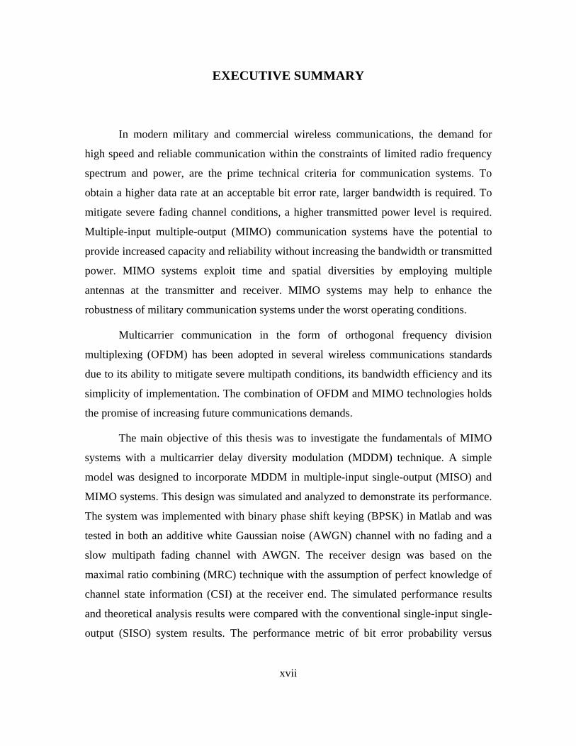
EXECUTIVE SUMMARY

In modern military and commercial wireless communications, the demand for

high speed and reliable communication within the constraints of limited radio frequency

spectrum and power, are the prime technical criteria for communication systems. To

obtain a higher data rate at an acceptable bit error rate, larger bandwidth is required. To

mitigate severe fading channel conditions, a higher transmitted power level is required.

Multiple-input multiple-output (MIMO) communication systems have the potential to

provide increased capacity and reliability without increasing the bandwidth or transmitted

power. MIMO systems exploit time and spatial diversities by employing multiple

antennas at the transmitter and receiver. MIMO systems may help to enhance the

robustness of military communication systems under the worst operating conditions.

Multicarrier communication in the form of orthogonal frequency division

multiplexing (OFDM) has been adopted in several wireless communications standards

due to its ability to mitigate severe multipath conditions, its bandwidth efficiency and its

simplicity of implementation. The combination of OFDM and MIMO technologies holds

the promise of increasing future communications demands.

The main objective of this thesis was to investigate the fundamentals of MIMO

systems with a multicarrier delay diversity modulation (MDDM) technique. A simple

model was designed to incorporate MDDM in multiple-input single-output (MISO) and

MIMO systems. This design was simulated and analyzed to demonstrate its performance.

The system was implemented with binary phase shift keying (BPSK) in Matlab and was

tested in both an additive white Gaussian noise (AWGN) channel with no fading and a

slow multipath fading channel with AWGN. The receiver design was based on the

maximal ratio combining (MRC) technique with the assumption of perfect knowledge of

channel state information (CSI) at the receiver end. The simulated performance results

and theoretical analysis results were compared with the conventional single-input single-

output (SISO) system results. The performance metric of bit error probability versus

xviii

0/bE N (energy per bit to noise power spectral density ratio) was used. To establish a

fair comparison, the transmitted power for the SISO, MISO and MIMO systems was

maintained equal.

The results showed that the designed MISO and MIMO system performed within

expected parameters of the theoretical analysis in both the AWGN channel with no

fading and the multipath fading channel with AWGN. The comparison of performances

in the AWGN channel with no fading showed that the MISO system performed better

than the SISO system for low 0/bE N values up to 6.5 dB and the performance of the

MISO system was poorer for higher 0/bE N values. The performances of the MIMO

systems were better than that of the SISO system for all values of 0/bE N and all

systems studies herein. The MIMO systems with two receive antennas and three receive

antennas outperformed a SISO system by 1.7 dB and 3.4 dB less transmit power required

respectively for equal performance. For the multipath fading channel with AWGN, the

MISO and MIMO systems were able to achieve significant advantage over a SISO

system.

1

I. INTRODUCTION

A. BACKGROUND One of the major challenges facing modern communications is to satisfy the ever

increasing demand of high speed reliable communications with the constraints of

extremely limited frequency spectrum and limited power. Wireless communications

systems like cellular mobile communications, internet and multimedia services require

very high capacity to fulfill the demand of high data rates. These systems must achieve

the desired reliability within the limits of power and frequency spectrum availability,

often in severe channel environments. They need to overcome signal scattering and

multipath effects, especially in densely populated urban areas. For many military

commutation systems, reliable communication is to be achieved with low probability of

detection and interception even in hostile jamming environments.

The solutions to achieve high capacity with reliability could include time,

frequency and space diversity. Wireless communication systems with multiple transmit

and multiple receive antennas can provide high capacity at low probability of bit error

with extremely low power, even in dense scattering and multipath environments. These

multiple-input multiple-output (MIMO) systems with appropriate space-time codes have

been an area of recent research as they hold the promise of ever increasing data rates. The

capacity of a MIMO system can be increased linearly by increasing the number of

transmit and receive antennas. The applications of MIMO systems in a frequency

selective channel require equalization and other techniques to compensate for frequency

selectivity of the channel, which add to the complexity of these systems. In recent years,

orthogonal frequency division multiplexing (OFDM) has been widely used in

communications systems to operate in frequency selective channels including several

wireless communication standards. Communication systems with a MIMO-OFDM

combination can significantly improve capacity and reliability by exploiting the

robustness of OFDM to fading, enhanced by adding more diversity gain via space time

codes. In this research, delay diversity in combination with a MIMO-OFDM system is

the primary focus and is referred to as multicarrier delay diversity modulation (MDDM).

[1, 2]

2

B. OBJECTIVE AND METHODOLOGY The main objective of this research was to investigate MIMO-OFDM systems by

using a cyclic delay diversity technique as a space time code and compare its

performance to conventional single-input single-output (SISO) systems. The first step to

achieve the objective was to study the fundamentals of OFDM systems. Then, the OFDM

technique was applied to a multiple-input single-output (MISO) system and MIMO

systems with cyclic delay diversity. A MISO system and two MIMO systems, using a

MDDM scheme with two transmit antennas, were simulated in Matlab with one, two and

three receive antennas, respectively. Multicarrier delay diversity was implemented with

binary phase shift keying (BPSK) and was realized in equivalent baseband form to

facilitate comparison with published theory. The design was simulated both with an

additive white Gaussian noise (AWGN) channel with no fading and then with a multipath

faded channel with AWGN. Theoretical performance and simulated system performance

were compared with reference to the single-input single-output (SISO) system.

C. RELATED RESEARCH MIMO systems promise high efficiency in providing low probability of bit error

without increasing the transmitted power or the bandwidth [1]. Therefore, research in this

area has been very active during recent years. The performance of MIMO systems

applying techniques such as delay diversity, space-time block codes (STBC) and space-

time trellis codes (STTC) has led to the development of several practical systems [1, 2].

Numerous studies have been performed to realize and investigate the performance of

these systems. Space time codes were originally developed for flat fading channels.

Later, incorporation of OFDM in these systems has provided a solution to

communications in the frequency selective channel [1]. Delay diversity was the first

diversity technique introduced for MIMO systems and was described in [3] and [4]. The

use of delay diversity with OFDM was proposed in [5] for a flat fading channel and a

cyclic delay diversity approach with OFDM was recommended for the frequency

selective fading channel in [6] which has been further investigated in [2].

D. THESIS ORGANIZATION This thesis is organized in five chapters. Chapter II introduces the fundamentals

of MIMO systems and the multicarrier delay diversity modulation scheme. It discusses

3

the capacity of MIMO systems, space time coding and use of time delay diversity as a

space time coding technique in MIMO systems. Chapter III describes the modeling and

simulation of the MDDM transmitter and receiver. Chapter IV analyzes the performance

of this modulation technique both in an AWGN channel with no fading and in a slow

fading multipath channel with AWGN. Chapter V reviews the summary of the work done

with results and includes recommendations for future study. Matlab code is attached as an

Appendix.

4


5

II. MIMO SYSTEMS AND MULTICARRIER DELAY DIVERSITY

The objective of this chapter is to establish the basic understanding of MIMO

systems, space time coding and the application of MDDM in MIMO systems. An

overview of the MIMO model is presented. The fundamentals of OFDM and its

implementations with the discrete Fourier transform (DFT) are discussed. Then, the

implementation of cyclic delay diversity with OFDM within the context of MIMO

systems is presented. Finally, the multipath flat fading channel and the maximum ratio

combining receiver are discussed.

A. MULTIPLE-INPUT MULTIPLE-OUTPUT (MIMO) SYSTEMS In order to facilitate the understanding of multiple-input multiple-output systems,

single-input single-output (SISO) systems, single-input multiple-output (SIMO) systems

and multiple-input single-output (MISO) systems models are discussed briefly. In this

thesis, all signals and models are represented in complex baseband equivalent form to

facilitate analysis.

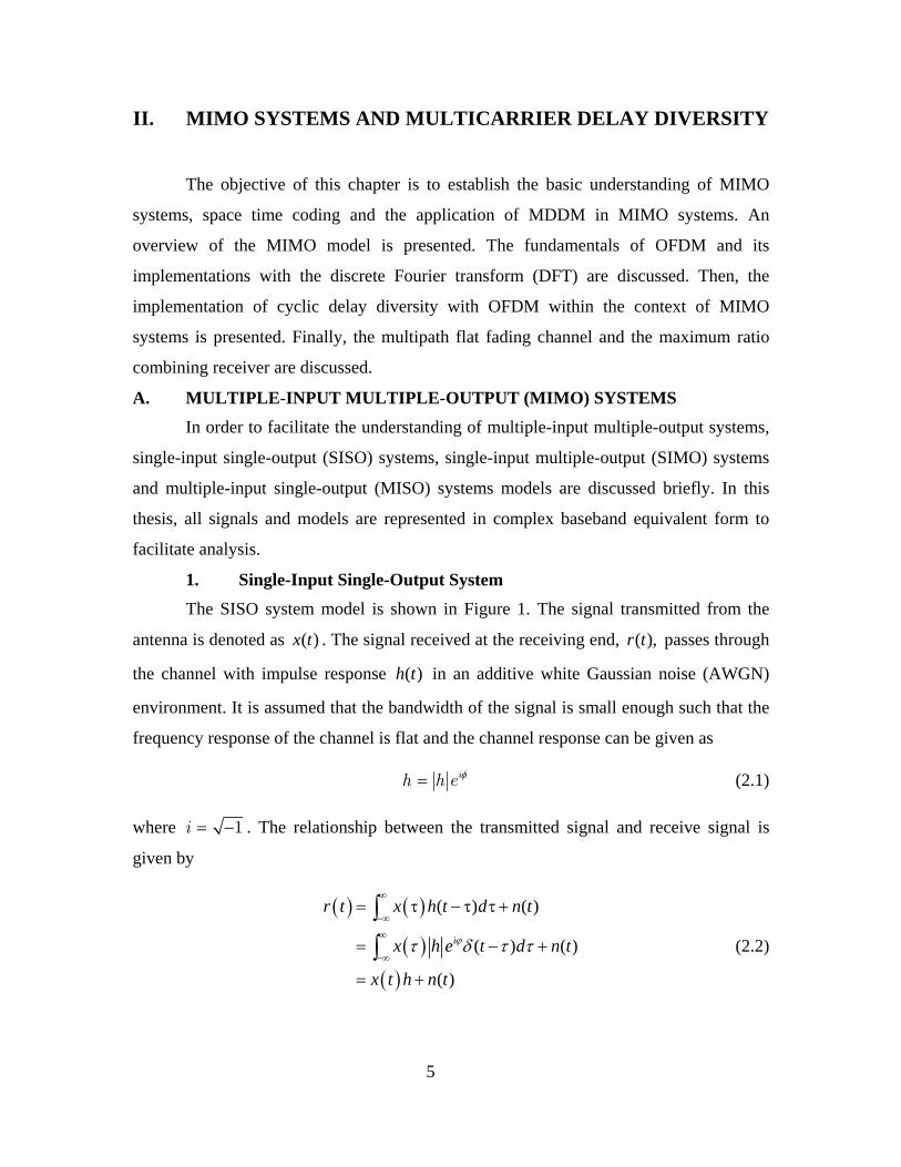
1. Single-Input Single-Output System The SISO system model is shown in Figure 1. The signal transmitted from the

antenna is denoted as ( )x t . The signal received at the receiving end, ( ),r t passes through

the channel with impulse response ( )h t in an additive white Gaussian noise (AWGN)

environment. It is assumed that the bandwidth of the signal is small enough such that the

frequency response of the channel is flat and the channel response can be given as

ih h e φ= (2.1)

where 1i = − . The relationship between the transmitted signal and receive signal is

given by

( ) ( )

( )( )

( ) ( )

( ) ( )

( )

ϕτ δ τ τ

∞

−∞

∞

−∞

= τ − τ τ +

= − +

= +

∫∫ i

r t x h t d n t

x h e t d n t

x t h n t

(2.2)

6

where ( )tδ is the Dirac delta function and ( )n t is the AWGN. The received signal is the

transmitted signal convolved with the channel impulse response plus added noise. [7]

( )r tTransmitter Receiver

( )h t

( )x t

Figure 1 SISO System (After Ref. [7])

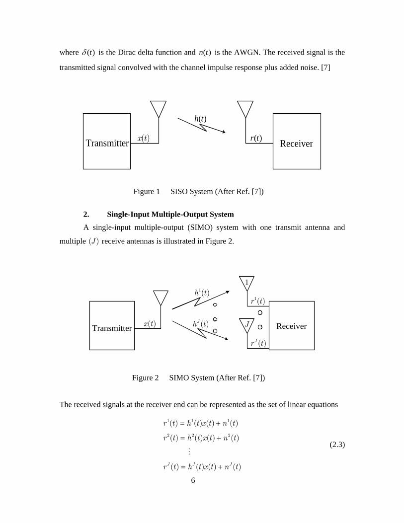
2. Single-Input Multiple-Output System A single-input multiple-output (SIMO) system with one transmit antenna and

multiple ( )J receive antennas is illustrated in Figure 2.

( )x t

1( )r t

1( )h t

( )Jr t

( )Jh tTransmitter Receiver

1

J

Figure 2 SIMO System (After Ref. [7])

The received signals at the receiver end can be represented as the set of linear equations

1 1 1

2 2 2

( ) ( ) ( ) ( )

( ) ( ) ( ) ( )

( ) ( ) ( ) ( )J J J

r t h t x t n t

r t h t x t n t

r t h t x t n t

= +

= +

= +

(2.3)

7

where ( )jr t , ( )jh t and ( )jn t , 1,2, 3,...,j J= represent the received signal, channel

impulse response and noise, respectively, at the -thj receive antenna. If

( ), ( ) and ( ) x t h t r t are sampled at the rate of one sample per symbol, then they can be

represented as , , x h r . The received signal can also be represented in form of vectors.

1 2 1 2 for ...⎡ ⎤= = = =⎣ ⎦TJ Jx x x x x xx (2.4)

1 2⎡ ⎤= ⎣ ⎦TJh h hh

1 2⎡ ⎤= ⎣ ⎦TJn n nn (2.5)

Now, the received vector is represented as

r = h.x + n (2.6)

where and x, h n are transmission, channel and noise vectors, respectively and operator

' '. denotes element by element multiplication.

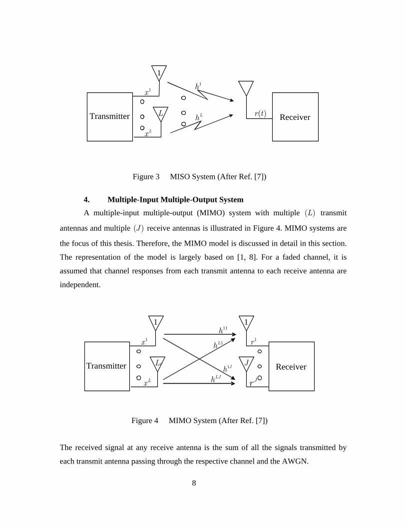
3. Multiple-Input Single-Output System

A multiple-input single-output (MISO) system with multiple ( )L transmit

antennas and one receive antenna is illustrated in Figure 3. The receive antenna receives a

sum of all the signals transmitted by each antenna and can be represented as

1 1 2 2 ... L Lr h x h x h x n= + + + + (2.7)

where and , 1,2,3,...,l lx h l L= are the transmitted signal and channel response from

transmit antenna l to the receive antenna and n is the AWGN. Equation (2.7) can also be

written as

1

Ll l

l

r h x n=

= +∑ . (2.8)

8

1x

( )r t

1h

Lx

LhTransmitter Receiver

1

L

Figure 3 MISO System (After Ref. [7])

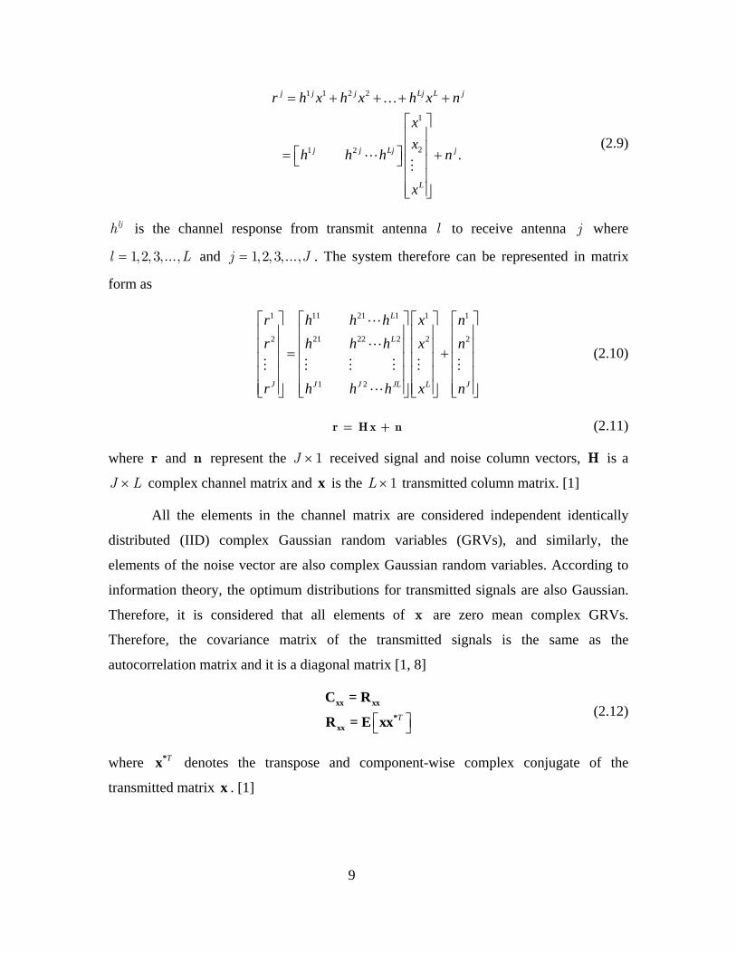
4. Multiple-Input Multiple-Output System

A multiple-input multiple-output (MIMO) system with multiple ( )L transmit

antennas and multiple ( )J receive antennas is illustrated in Figure 4. MIMO systems are

the focus of this thesis. Therefore, the MIMO model is discussed in detail in this section.

The representation of the model is largely based on [1, 8]. For a faded channel, it is

assumed that channel responses from each transmit antenna to each receive antenna are

independent.

11h1x

Lx

1r

JrLJh

1Lh

1JhTransmitter Receiver

1

J

1

t L

Figure 4 MIMO System (After Ref. [7])

The received signal at any receive antenna is the sum of all the signals transmitted by

each transmit antenna passing through the respective channel and the AWGN.

9

1 1 2 2

1

21 2 .

= + + + +

⎡ ⎤⎢ ⎥⎢ ⎥⎡ ⎤= +⎣ ⎦ ⎢ ⎥⎢ ⎥⎢ ⎥⎣ ⎦

…j j j Lj L j

j j Lj j

L

r h x h x h x n

xx

h h h n

x

(2.9)

ljh is the channel response from transmit antenna l to receive antenna j where

1,2, 3,...,l L= and 1,2, 3,...,j J= . The system therefore can be represented in matrix

form as

1 11 21 1 1 1

2 21 22 2 2 2

1 2

⎡ ⎤ ⎡ ⎤ ⎡ ⎤ ⎡ ⎤⎢ ⎥ ⎢ ⎥ ⎢ ⎥ ⎢ ⎥⎢ ⎥ ⎢ ⎥ ⎢ ⎥ ⎢ ⎥= +⎢ ⎥ ⎢ ⎥ ⎢ ⎥ ⎢ ⎥⎢ ⎥ ⎢ ⎥ ⎢ ⎥ ⎢ ⎥⎢ ⎥ ⎢ ⎥ ⎢ ⎥ ⎢ ⎥⎣ ⎦ ⎣ ⎦ ⎣ ⎦ ⎣ ⎦

L

L

J J J JL L J

r h h h x nr h h h x n

r h h h x n

(2.10)

r = Hx + n (2.11)

where r and n represent the 1J × received signal and noise column vectors, H is a

J L× complex channel matrix and x is the 1L × transmitted column matrix. [1]

All the elements in the channel matrix are considered independent identically

distributed (IID) complex Gaussian random variables (GRVs), and similarly, the

elements of the noise vector are also complex Gaussian random variables. According to

information theory, the optimum distributions for transmitted signals are also Gaussian.

Therefore, it is considered that all elements of x are zero mean complex GRVs.

Therefore, the covariance matrix of the transmitted signals is the same as the

autocorrelation matrix and it is a diagonal matrix [1, 8]

⎡ ⎤⎣ ⎦

T

xx xx

*xx

C = R

R = E xx (2.12)

where T*x denotes the transpose and component-wise complex conjugate of the

transmitted matrix x . [1]

10

The total transmitted power, P , is the sum of all the diagonal elements of the

autocorrelation matrix. To facilitate the analysis for the MIMO system, assume that all

the transmit antennas transmit equal power [8].

( )2 2

1 1

E E tr= =

⎡ ⎤ ⎡ ⎤= = =⎢ ⎥ ⎢ ⎥⎣ ⎦⎣ ⎦∑ ∑

L Ll l

xxl l

P x x R (2.13)

2

El l PP x

L⎡ ⎤= =⎣ ⎦ (2.14)

where lP is the average power transmitted from antenna l . An AWGN channel is

considered, and according to information theory, the optimum distribution for the

transmitted signal is also Gaussian [1]. Therefore, the elements of x as stated in [1] are

also considered independent and identically distributed (IID) Gaussian variables with

zero mean. Then, the autocorrelation matrix can be written as

=xx LPL

R I (2.15)

where LI is the identity matrix of sizeL L× .

It is further assumed that the channel matrix is fixed at least for the duration of

one symbol period and there is no attenuation due to path loss and no amplification due to

antenna gain. In other words, each receive antenna receives the total transmitted power

regardless of its branch. Thus, the normalization constraint for the elements of channel

matrix H for fixed coefficient can be represented as [1]

2

1for 1,2,

=

= =∑ …L

jl

lh L j J . (2.16)

For a faded channel, the channel matrix elements are random variables and the

normalization constraint will apply to the expected value of Equation (2.16). This

normalization constraint is required for a fair comparison with SISO systems with equal

power transmitted [8]. It is also assumed that the channel impulse response at that time,

referred to as the channel state information (CSI), is perfectly known at the receiver by

sending training symbols. [1]

11

The elements of the noise vector n are considered IID complex Gaussian random

variables with zero mean and the variance of 2 /2oσ for both real and imaginary parts.

Independence of the noise elements and zero mean imply that the autocorrelation and

covariance matrix are the same diagonal matrix. Therefore, the covariance matrix nnC of

the noise vector can be represented as [1, 8]

*E ⎡ ⎤⎣ ⎦= Tnn nn=C R nn (2.17)

2 .σ= o LnnR I (2.18)

The average signal power at receive antenna j with assumed fixed channel coefficients

can be given by [1, 8]

*

* *

1 1

* *

1 1

* *

1 1

2 2

1

E

E

E

E

E

= =

= =

= =

=

⎡ ⎤= ⎣ ⎦⎡ ⎤

= ⎢ ⎥⎣ ⎦⎡ ⎤

= ⎢ ⎥⎣ ⎦

⎡ ⎤= ⎣ ⎦

⎡ ⎤= ⎢ ⎥⎣ ⎦

∑ ∑

∑∑

∑∑

∑

j j jr

L Ll j l mj m

l m

L Ll j l mj m

l m

L Ll j l j j m

l mL

l j l

l

P r r

h x h x

h x h x

h h x x

h x

(2.19)

where *( ) denotes complex conjugate. Substitution of Equations (2.15) and (2.16) into

Equation (2.19) yields

2 2

1E .

=

⎡ ⎤= = =⎢ ⎥⎣ ⎦∑L

j l j lr

l

PP h x L PL

(2.20)

Then, the average signal-to-noise ratio (SNR) at each receive antenna, represented by γ ,

is given by [1, 8]

2 .γσ

=o

P (2.21)

Similarly, the autocorrelation matrix for the received signal can be represented as [8]

12

*E ⎡ ⎤⎣ ⎦= TrrR rr . (2.22)

( )( )

( ) ( )( )( ) ( )

( ) ( )

*

* *

* ** *

* ** *

E

E

E

E E E E .

⎡ ⎤= + +⎣ ⎦⎡ ⎤= + +⎣ ⎦⎡ ⎤= + + +⎣ ⎦⎡ ⎤ ⎡ ⎤⎡ ⎤ ⎡ ⎤= + + +⎣ ⎦ ⎣ ⎦⎣ ⎦ ⎣ ⎦

Trr

T T

T TT T

T TT T

R Hx n Hx n

Hx n Hx n

Hx Hx Hxn n Hx nn

Hx Hx Hxn Hx n nn

(2.23)

By using the identity of transposition of a product of matrices [9] as follows

( )* * *T T T=Hx x H . (2.24)

Equation (2.23) can be written as

* * * * * *E E E E⎡ ⎤ ⎡ ⎤ ⎡ ⎤ ⎡ ⎤= + + +⎣ ⎦ ⎣ ⎦ ⎣ ⎦ ⎣ ⎦T T T T T T

rrR Hxx H Hxn x H n nn . (2.25)

If it is assumed that the channel coefficients are deterministic and signal matrix x and

noise matrix n are independent with zero mean, Equation (2.25) yields

* * *

*

E E

.

⎡ ⎤ ⎡ ⎤= +⎣ ⎦ ⎣ ⎦= +

T T Trr

Txx nn

R H xx H nn

HR H R (2.26)

B. SPACE TIME CODING Space time coding is a technique to achieve higher diversity at the receiver end to

mitigate multipath fading without increasing the transmitted power or bandwidth. Space

time coding holds the promise to maximize the system capacity. The system capacity is

defined in [1], “The maximum possible transmission rate such that the probability of

error is arbitrarily small.” The capacity of SISO system is given by Shannon’s capacity

equation [10]

2

2 2

log (1 )

log 1

C W SNR

PC W

σ

= +

⎛ ⎞= +⎜ ⎟⎝ ⎠

(2.27)

where C ,W ,P and 2σ represent capacity, bandwidth, average signal power and average

noise power, respectively. The capacity of a MIMO system in a flat fading channel with

perfect channel state information is given by [1]

13

2 2log 1 .σ

⎛ ⎞= +⎜ ⎟⎝ ⎠

PC W LJ (2.28)

Space time coding techniques designed appropriately with MIMO systems have

the potential to achieve the channel capacity in Equation (2.28). Space time coding

provides the diversity both in time and space to achieve the higher performance at

reduced transmitted power and without bandwidth expansion. Space time coding

techniques can be classified into two main categories. The first category provides power

efficiency without compromising the performance such as delay diversity, space-time

block codes (STBC) and space-time turbo trellis codes (STTC). The other category, such

as Bell Labs layered space-time technology (BLAST), increases the data rates with the

use of bandwidth efficient modulation schemes [2].

The performance of a MIMO system can be further improved by applying

forward error correction coding (FEC) with optimum interleaving at the cost of reduced

data rate or increased bandwidth. FEC coding gain can be achieved without sacrificing

the data rate or bandwidth by designing space time coding technique with higher rate

modulation schemes. [1]

This thesis is focused on achieving multicarrier delay diversity gain. The

incorporation of error control coding and interleaving is left for future work.

C. MULTICARRIER DELAY DIVERSITY IN MIMO SYSTEMS The delay diversity technique was the first approach proposed for MIMO systems

[2]. In this scheme, delayed versions of the same signal are transmitted by multiple

antennas. This simple delay diversity was originally suggested for flat fading channels

[11]. This scheme has the inherent problem of increasing frequency selectivity caused by

the delay diversity. Full diversity cannot be achieved without equalization [12] and

equalization for MIMO systems is very difficult due to the large number of channels.

Thus, the receiver design becomes much more complicated. Orthogonal frequency

division multiplexing (OFDM) with delay diversity is another approach to make good use

of frequency selectivity of the delay diversity. The OFDM scheme with delay diversity

has a limitation as an increase in the number of transmit antennas requires an increase in

14

the guard interval at the expense of bandwidth. If the guard interval is not as large as or

larger than the delay spread of the channels, then it will cause inter-symbol interference

(ISI) [12].

The OFDM scheme can be easily implemented by using the inverse discrete

Fourier transform (IDFT), which can be efficiently computed by the inverse fast Fourier

transform (IFFT). The same information can be translated back by the DFT operation.

DFT and IDFT as defined in [13] are

[ ]{ } [ ] [ ] π−

−

=

= = =∑1

2 /

0

DFT for 0,1,2,..., - 1N

i kn N

n

x m X k x m e k N (2.29)

[ ]{ } [ ] [ ] π−

=

= = =∑1

2 /

0

1IDFT for 0,1,2,..., - 1

Ni kn N

k

X k x m X k e m NN

. (2.30)

Discrete Fourier transforms have a property that any circular shift in the time domain

results in a phase shift in the frequency domain [13]

[ ]{ } [ ]π−− = = −2 /DFT ( ) for 0,1,2,..., 1i kD NNx m D e X k k N (2.31)

where D denotes the delay in the time index and ( )Nn denotes n modulo N . This cyclic

delay property of the Fourier transforms can be used in an OFDM system design to

induce diversity that can be exploited at the receiver end.

To overcome the problems of a simple time delay diversity scheme in a frequency

selective fading channel for MIMO-OFDM systems, a new approach of cyclic delay

diversity was suggested in [6]. This simple scheme does not require any additional guard

interval with an increasing number of transmit antennas. The combination of cyclic delay

diversity and OFDM in MIMO systems has been referred to as multicarrier delay

diversity modulation (MDDM) in this thesis and this can be considered a special type of

space-time coding. For a frequency selective channel, a cyclic guard interval (cyclic

prefix) of duration G is added at the beginning of each OFDM symbol. This guard

interval is greater than or equal to the maximum channel delay M to mitigate the

intersymbol interference (ISI). The orthogonality of subcarriers is paramount for OFDM.

The cyclic prefix converts a linear convolution channel into a circular convolution

channel and the interference from the previous symbols will only affect the guard

15

interval. This restores the orthogonality at the receiver. Adding zeros as the guard interval

can alleviate the interference between OFDM symbols. For a flat fading channel, the

guard interval can be eliminated to increase the data rate. [2, 22]

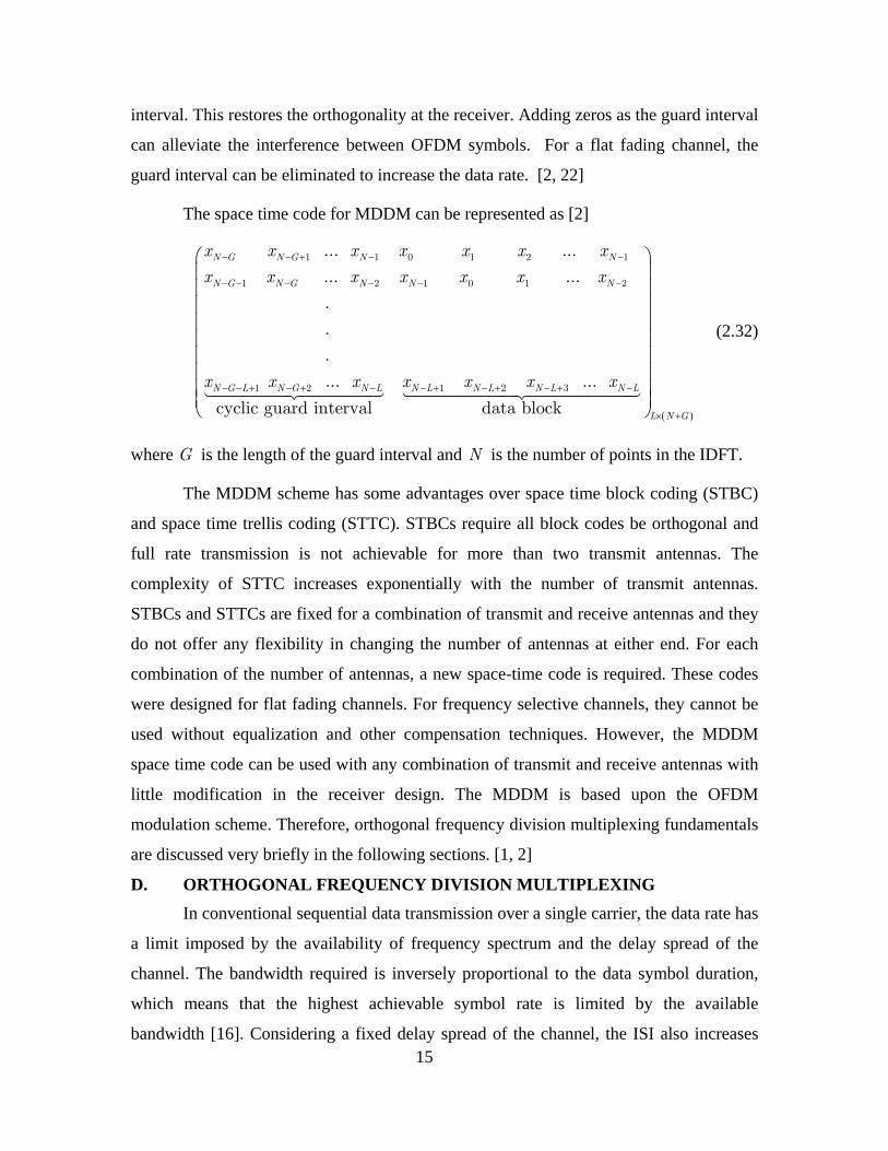
The space time code for MDDM can be represented as [2]

1 1 0 1 2 1

1 2 1 0 1 2

... ...

... ...

.

.

.

N G N G N N

N G N G N N N

N

x x x x x x x

x x x x x x x

x

− − + − −

− − − − − −

−

( )

1 2 1 2 3 ... ...

cyclic guard interval data blockG L N G N L N L N L N L N L

L N G

x x x x x x− + − + − − + − + − + −

× +

⎛ ⎞⎜ ⎟⎜ ⎟⎜ ⎟⎜ ⎟⎜ ⎟⎜ ⎟⎜ ⎟⎜ ⎟⎜ ⎟⎝ ⎠

(2.32)

where G is the length of the guard interval and N is the number of points in the IDFT.

The MDDM scheme has some advantages over space time block coding (STBC)

and space time trellis coding (STTC). STBCs require all block codes be orthogonal and

full rate transmission is not achievable for more than two transmit antennas. The

complexity of STTC increases exponentially with the number of transmit antennas.

STBCs and STTCs are fixed for a combination of transmit and receive antennas and they

do not offer any flexibility in changing the number of antennas at either end. For each

combination of the number of antennas, a new space-time code is required. These codes

were designed for flat fading channels. For frequency selective channels, they cannot be

used without equalization and other compensation techniques. However, the MDDM

space time code can be used with any combination of transmit and receive antennas with

little modification in the receiver design. The MDDM is based upon the OFDM

modulation scheme. Therefore, orthogonal frequency division multiplexing fundamentals

are discussed very briefly in the following sections. [1, 2]

D. ORTHOGONAL FREQUENCY DIVISION MULTIPLEXING In conventional sequential data transmission over a single carrier, the data rate has

a limit imposed by the availability of frequency spectrum and the delay spread of the

channel. The bandwidth required is inversely proportional to the data symbol duration,

which means that the highest achievable symbol rate is limited by the available

bandwidth [16]. Considering a fixed delay spread of the channel, the ISI also increases

16

with the increase in the symbol rate as delayed copies of the symbols coming from the

multipath can have significant overlap with the original symbol. The lessening of ISI will

require equalization which further adds to the complexity of the system [17]. These

problems can be mitigated by transmitting the data in parallel on multiple carriers with a

reduced data rate on each carrier compared to the overall data rate. The reduced data rate

will require reduced bandwidth which should not be more than the coherence bandwidth

of the channel to avoid frequency selective fading. This multicarrier system can be

designed by classical frequency division multiplexing (FDM) [1]. In this scheme, the

carriers need to be well apart in frequency domain to avoid inter-carrier interference.

Therefore, a guard frequency band is required between two consecutive subcarriers which

makes this scheme highly inefficient in frequency spectrum utilization. This problem can

be eliminated by using minimum-spaced orthogonal carriers. In OFDM, all carriers are

allowed to overlap by maintaining orthogonality of all the subcarriers, which increases

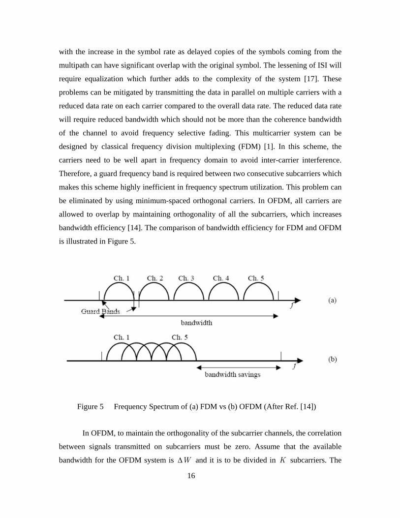
bandwidth efficiency [14]. The comparison of bandwidth efficiency for FDM and OFDM

is illustrated in Figure 5.

Figure 5 Frequency Spectrum of (a) FDM vs (b) OFDM (After Ref. [14])

In OFDM, to maintain the orthogonality of the subcarrier channels, the correlation

between signals transmitted on subcarriers must be zero. Assume that the available

bandwidth for the OFDM system is W∆ and it is to be divided in K subcarriers. The

17

input serial data stream is to be converted into K parallel data streams which are

assigned to the K subcarriers [1]. The symbol duration of the input serial data is 'sT with

serial data rate of ''

1s

s

fT

= . Therefore, if the number of parallel data streams is equal to

the number of OFDM subcarriers, the symbol duration for OFDM will be

= '.s sT KT (2.33)

Equation (2.33) indicates that the symbol duration of an OFDM signal is K times larger

than that of single serial stream symbol duration. Therefore, the OFDM scheme has the

inherited advantage over single carrier modulation techniques to mitigate ISI and

frequency selectivity of the channel. The OFDM transmitted signal ( )S t can be written

as

{ }1

0

1

2 2 2 20

( ) cos(2 ) sin(2 )

= cos(2 ) sin(2 )

m m

m m

m m m m

K

I m Q mm

KI Q

m m mm I Q I Q

S t A d f t d f t

d da f t f t

d d d d

π π

π π

−

=

−

=

= −

⎧ ⎫⎪ ⎪−⎨ ⎬+ +⎪ ⎪⎩ ⎭

∑

∑ (2.34)

where A is a constant, mId ,

mQd are the information-bearing components of the signal

and 2 2( )m mm I Qa A d d= + .

Using the trigonometric identity

cos( ) cos( )cos( ) sin( )sin( )α β α β α β+ = − (2.35)

( )S t can be written as

{ }

1

0

1

0

( ) cos(2 )

cos(2 )cos( ) sin(2 )sin( )

K

m m mm

K

m m m m mm

S t a f t

a f t f t

π θ

π θ π θ

−

=

−

=

= +

= −

∑

∑ (2.36)

18

where 1m tan m

m

Q

I

ddθ − ⎛ ⎞= ⎜ ⎟

⎝ ⎠. The correlation between any two symbols transmitted on

separate subcarriers, represented as ijR , must be equal to zero to maintain the

orthogonality of subcarriers [1].

0

( ) ( )

cos(2 ) cos(2 )s

ij i j

T

i i i j j j

R s t s t dt

a f t t a f t t dtπ θ π θ

+∞

−∞=

= + +

∫∫

(2.37)

Using the trigonometric identity

1 1cos( )cos( ) cos( ) cos( )

2 2α β α β α β= + + − . (2.38)


( )0

cos(2 ( ) ( ) ) cos(2 ( ) ( ) )2

sTi jij i j i j i j i j

a aR f f t t f f t t dtπ θ θ π θ θ= + + + + − + −∫ (2.39)

where , , i j i ja a q and q are constant for the symbol duration.

For 12 ( )i j

s

f fT

π + , Equation (2.39) can be written as

0

cos(2 ( ) ( ) )2

sTi jij i j i j

a aR f f t t dtπ θ θ= − + −∫ . (2.40)

From Equation (2.40), 0ijR = if

( ) where set of positive integers

/ .

i j s

i j s

f f T M M

f f M T

− = ∈

⇒ − = (2.41)

Therefore, minimum frequency separation between two consecutive subcarriers to

maintain orthogonality must be

1 s

s

f fT

= = (2.42)

where sf is the rate of OFDM symbols.

19

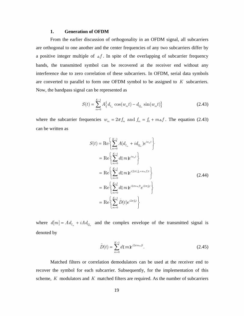
1. Generation of OFDM From the earlier discussion of orthogonality in an OFDM signal, all subcarriers

are orthogonal to one another and the center frequencies of any two subcarriers differ by

a positive integer multiple of f . In spite of the overlapping of subcarrier frequency

bands, the transmitted symbol can be recovered at the receiver end without any

interference due to zero correlation of these subcarriers. In OFDM, serial data symbols

are converted to parallel to form one OFDM symbol to be assigned to K subcarriers.

Now, the bandpass signal can be represented as

{ }1

0

( ) cos( ) sin( )m m

K

I m Q mm

S t A d w t d w t−

=

= −∑ (2.43)

where the subcarrier frequencies 02 and m m mw f f f m fπ= = + . The equation (2.43)

can be written as

[ ]

[ ]

[ ]

0

0

0

1

0

1

0

1(2 ( )

0

12 2

0

12

0

( ) Re ( )

Re

Re

Re

Re ( )

m

m m

m

Kiw t

I Qm

Kiw t

m

Ki f m f t

m

Ki n ft i f t

m

Ki f t

m

S t A d id e

d m e

d m e

d m e e

D t e

π

π π

π

−

=

−

=

−+

=

−

=

−

=

⎧ ⎫= +⎨ ⎬

⎩ ⎭⎧ ⎫

= ⎨ ⎬⎩ ⎭⎧ ⎫

= ⎨ ⎬⎩ ⎭⎧ ⎫

= ⎨ ⎬⎩ ⎭⎧ ⎫

= ⎨ ⎬⎩ ⎭

∑

∑

∑

∑

∑∼

(2.44)

where [ ]m mI Qd m Ad iAd= + and the complex envelope of the transmitted signal is

denoted by

[ ]1

2

0

( ) .K

i m ft

m

D t d m e π−

=

= ∑∼

(2.45)

Matched filters or correlation demodulators can be used at the receiver end to

recover the symbol for each subcarrier. Subsequently, for the implementation of this

scheme, K modulators and K matched filters are required. As the number of subcarriers

20

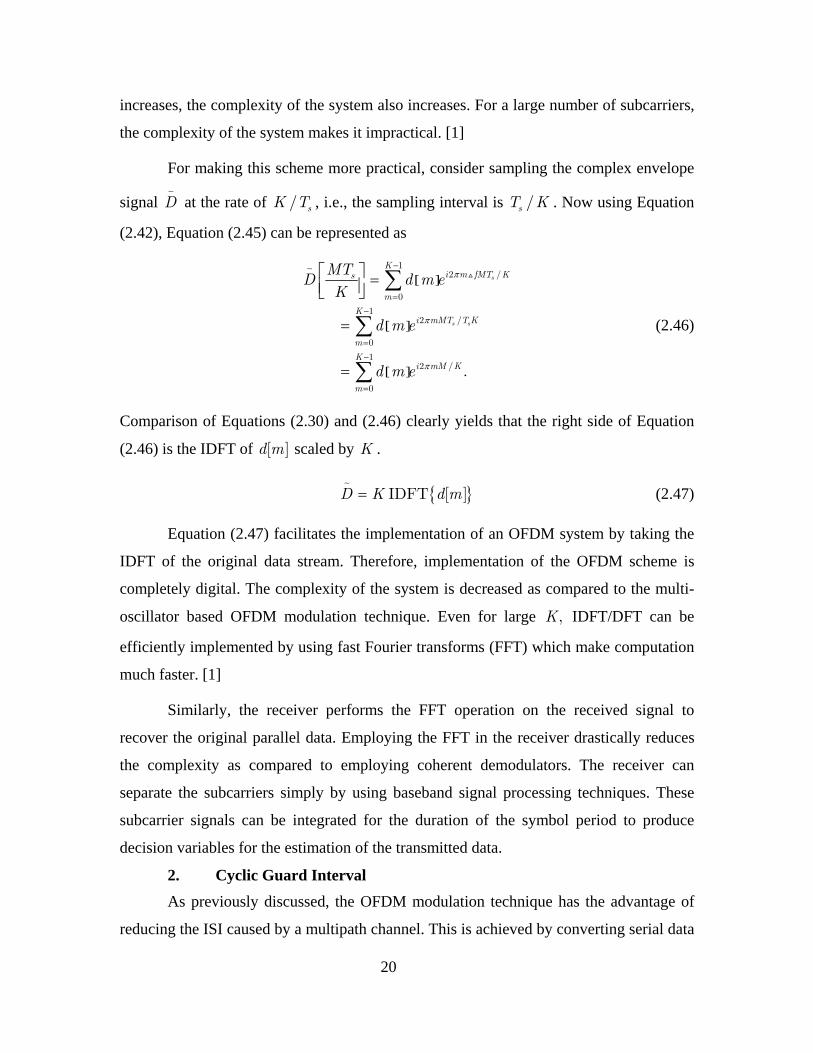
increases, the complexity of the system also increases. For a large number of subcarriers,

the complexity of the system makes it impractical. [1]

For making this scheme more practical, consider sampling the complex envelope

signal D∼

at the rate of / sK T , i.e., the sampling interval is /sT K . Now using Equation

(2.42), Equation (2.45) can be represented as

[ ]

[ ]

[ ]

12 /

0

12 /

0

12 /

0

.

s

s s

Ki m fMT Ks

m

Ki mMT T K

m

Ki mM K

m

MTD d m eK

d m e

d m e

π

π

π

−

=

−

=

−

=

⎡ ⎤ =⎢ ⎥⎣ ⎦

=

=

∑

∑

∑

∼

(2.46)

Comparison of Equations (2.30) and (2.46) clearly yields that the right side of Equation

(2.46) is the IDFT of [ ]d m scaled by K .

{ }=∼

IDFT [ ]D K d m (2.47)

Equation (2.47) facilitates the implementation of an OFDM system by taking the

IDFT of the original data stream. Therefore, implementation of the OFDM scheme is

completely digital. The complexity of the system is decreased as compared to the multi-

oscillator based OFDM modulation technique. Even for large ,K IDFT/DFT can be

efficiently implemented by using fast Fourier transforms (FFT) which make computation

much faster. [1]

Similarly, the receiver performs the FFT operation on the received signal to

recover the original parallel data. Employing the FFT in the receiver drastically reduces

the complexity as compared to employing coherent demodulators. The receiver can

separate the subcarriers simply by using baseband signal processing techniques. These

subcarrier signals can be integrated for the duration of the symbol period to produce

decision variables for the estimation of the transmitted data.

2. Cyclic Guard Interval As previously discussed, the OFDM modulation technique has the advantage of

reducing the ISI caused by a multipath channel. This is achieved by converting serial data

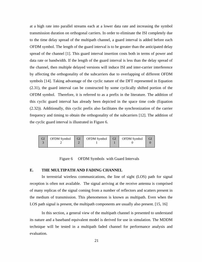
21

at a high rate into parallel streams each at a lower data rate and increasing the symbol

transmission duration on orthogonal carriers. In order to eliminate the ISI completely due

to the time delay spread of the multipath channel, a guard interval is added before each

OFDM symbol. The length of the guard interval is to be greater than the anticipated delay

spread of the channel [1]. This guard interval insertion costs both in terms of power and

data rate or bandwidth. If the length of the guard interval is less than the delay spread of

the channel, then multiple delayed versions will induce ISI and inter-carrier interference

by affecting the orthogonality of the subcarriers due to overlapping of different OFDM

symbols [14]. Taking advantage of the cyclic nature of the DFT represented in Equation

(2.31), the guard interval can be constructed by some cyclically shifted portion of the

OFDM symbol. Therefore, it is referred to as a prefix in the literature. The addition of

this cyclic guard interval has already been depicted in the space time code (Equation

(2.32)). Additionally, this cyclic prefix also facilitates the synchronization of the carrier

frequency and timing to obtain the orthogonality of the subcarriers [12]. The addition of

the cyclic guard interval is illustrated in Figure 6.

Figure 6 OFDM Symbols with Guard Intervals

E. THE MULTIPATH AND FADING CHANNEL

In terrestrial wireless communications, the line of sight (LOS) path for signal

reception is often not available. The signal arriving at the receive antenna is comprised

of many replicas of the signal coming from a number of reflectors and scatters present in

the medium of transmission. This phenomenon is known as multipath. Even when the

LOS path signal is present, the multipath components are usually also present. [15, 16]

In this section, a general view of the multipath channel is presented to understand

its nature and a baseband equivalent model is derived for use in simulation. The MDDM

technique will be tested in a multipath faded channel for performance analysis and

evaluation.

OFDM Symbol 1

GI 2

GI 1

GI 3

OFDM Symbol 0

OFDM Symbol 2

GI 0

22

In a multipath channel, the signal travels via several different paths before

arriving at the receive antenna. Due to the different path lengths involved, the amplitude

and phase of these received replicas are not the same. For example, if a short duration

pulse is transmitted in a multipath channel, then a train of pulses of different amplitudes,

phases and arrival times, will be received. As a result, the received signal can

significantly vary in amplitude and phase and the spectral components of the signal are

affected differently by the multipath faded channel. Therefore, the frequency response of

the channel may not be flat over the entire bandwidth of the signal. Multipath

components of the signal create time-spreading of the signal and cause intersymbol

interference. [15, 16]

The channel conditions may not remain constant over time and the media

composition (e.g., stratosphere, ionosphere) may also change. Furthermore, the number

and position of the reflectors and scatters cannot be considered fixed. In mobile

communications, due to the motion of transmitter and receiver, the multipath

arrangements can never be assumed constant and Doppler shift in signal frequency

proportional to the relative velocity is also observed. Therefore, the multipath fading

channel is a time varying channel [15]. Time varying and time spreading aspects of the

channel cannot be predicted or calculated precisely. For creating a good model of the

channel, these parameters are measured, and based on these measured statistics, the

channel can be characterized.

Doppler spread in the signal frequency describes the time varying nature of the

channel. The coherence time is inversely proportional to the Doppler shift. The coherence

time is the statistical measure over which the channel response does not change

significantly. To characterize the channel, the coherence time is compared with the

symbol duration. If the coherence time is less than the symbol durations, then the channel

is called a fast fading channel. In the case of coherence time greater than the symbol

duration, it is described as a slow fading channel. [15, 16]

The multipath delay spread is characterized by the coherence bandwidth.

Coherence bandwidth has been defined in [17] as, “a statistical measure over which the

frequency response of the channel is considered flat.” If the bandwidth of the signal is

23

greater than the coherence bandwidth of the channel, then different frequency

components will be attenuated differently and the phase variations will also be nonlinear.

This type of channel is said to be a frequency selective fading channel. If the coherence

bandwidth of the channel is greater than the signal bandwidth, then all the frequency

components will face flat fading with almost linear phase changes. This type of channel

is said to be a frequency nonselective fading channel. [15, 16]

This fading channel can be modeled statistically as there are a large number of

variables affecting the channel response. Most of these variables are random in nature

and several probability distributions can be considered to model these random variables

[16]. When there are a large number of reflectors and scatters in the physical channel, the

cumulative effect of this large number of random variables, as per the central limit

theorem, leads to a Gaussian process model for the channel response. In the case of no

LOS component present, the process has zero mean with magnitude following the

Rayleigh probability distribution and the phase is uniformly distributed on [ ] to π π− .

[15, 16]

1. Flat Rayleigh Fading Channel A slow fading frequency nonselective channel was simulated to test the

multicarrier delay diversity modulation scheme. The channel fading gain was kept fixed

for the symbol duration to make it a slow fading channel. Considering the no line of sight

(LOS) path case, a flat fading channel is usually simulated using a Rayleigh distribution

for the magnitude of the channel response [16]. The Rayleigh distribution is a special

case of the Ricean distribution with no line of sight component. The probability density

function for a Rayleigh random variable can be derived from the Ricean probability

density function as defined in [15]

2 2

02 2 2

( )( ) exp ( )

2c

c c cA c c

a a af a I u a

α ασ σ σ

⎛ − + ⎞ ⎛ ⎞= ⎜ ⎟⎜ ⎟ ⎝ ⎠⎝ ⎠ (2.48)

where ( )0 .I is the modified Bessel function of the first kind of zero order, (.)u is the

unit step function and 2α is the power in the LOS signal component and the average

received signal power is

24

2 2 2 2( ) 2cs t a α σ= = + (2.49)

1 0

( )0 0.

c

cc

au a

a

≥⎧⎪= ⎨ <⎪⎩ (2.50)

For the Rayleigh distribution case, there is no line of sight component so 0α = and

( )0 0 1I = . Using Equation (2.48), the Rayleigh probability density function can be

represented as

2

2 2( ) exp ( )2c

c cA c c

a af a u a

σ σ⎛ − ⎞

= ⎜ ⎟⎝ ⎠

. (2.51)

For the baseband simulation of a Rayleigh random variable, two zero mean

independent real Gaussian random variables were summed as X jY+ [17]. The

magnitude of this complex random quantity is the desired Rayleigh random variable and

simulates the magnitude of the channel frequency response. The derivation of the proof

that the complex sum of two zero mean Gaussian random variables has magnitude with

Rayleigh distribution and phase uniformly distributed in [ ], π π− is largely based on [8].

Let X and Y be two zero mean independent identically distributed (IID) Gaussian

random variables and their complex sum is represented by

Z X iY= + . (2.52)

As Z is to simulate the frequency response of a Rayleigh flat fading channel, it can be

written as

iZ he θ= (2.53)

2 2 2V Z X Y= = + . (2.54)

Since X and Y are zero mean IID Gaussian random variables (GRVs)

0X Y= = (2.55)

2 2 2X Yσ σ σ= = . (2.56)

25

The random variable V is a sum of two squared zero mean GRVs and is called a central

chi-squared random variable of degree 2. The probability density function for a central

chi-squared random variable of degree n can be given as [16]

( ) ( )2( / 2) 1 / 2

/ 2

1

22

σ

σ

− −=⎛ ⎞Γ⎜ ⎟⎝ ⎠

n vV

n nf v v e u v

n (2.57)

where n is the number of independent variables and ( ).Γ is the gamma function. For a

central chi-squared random variable of degree two ( 2n = ), Equation (2.57) can be

rewritten as

( ) ( ) ( )2/ 22

1 .2 1

σ

σ−=

Γv

Vf v e u v (2.58)

Since

( )1 (1 1)! 1Γ = − = , (2.59)

[15], the probability density function of V as per Equation (2.58) can be written as

( ) ( )2/ 22

12

σ

σ−= v

Vf v e u v . (2.60)

The magnitude of the simulated Rayleigh flat faded channel frequency response can be

written as

= =h Z V (2.61)

The probability density function for h can be obtained by transforming the probability

density function of V given in Equation (2.58) according to [18]

( )2

1 ( )/

=

=H V

v h

f h f vdh dv

(2.62)

where

( )1/ 2

12

=dhdv v

. (2.63)

26

Substituting Equations (2.60) and (2.63) into Equation (2.62) yields

( ) ( )

( ) ( )

2 2

2 2

2 1/ 2 / 22

/ 22

12( )2

.

σ

σ

σ

σ

−

−

=

=

hH

hH

f h h e u h

hf h e u h (2.64)

Comparison of Equations (2.51) and (2.64) clearly indicates that the magnitude of the

complex sum of two zero mean IID GRVs follows the Rayleigh distribution. The mean

and variance of h as given in [18] are

2πσ=h (2.65)

2 2 2 .2πσ σ ⎛ ⎞= −⎜ ⎟

⎝ ⎠h (2.66)

Now, the probability distribution function for the phase, θ , of Z is to be derived.

The phase θ can be represented as [8]

( )

( )

( )

1

1

1

tan if 0 and 0 referred to as case A

tan if 0 and referred to as case B

tan if 0 and 0 referred to as case C

Y X YXY X YXY X YX

π

θ

π

−

−

−

⎧ ⎛ ⎞ − −∞ < < −∞ < ≤⎜ ⎟⎪ ⎝ ⎠⎪⎪ ⎛ ⎞= < < ∞ −∞ < < ∞⎨ ⎜ ⎟

⎝ ⎠⎪⎪ ⎛ ⎞ + −∞ < < ≤ < ∞⎪ ⎜ ⎟

⎝ ⎠⎩

(2.67)

Let the ratio of zero mean IID GRVs X and Y be defined as [8, 19]

=YRX

. (2.68)

The joint probability density function of X and Y can be written as

( ) ( ) ( ) , ( ) ( )XY X Y X Xf x y f x f y f x f y= = (2.69)

where

( )2

222

1

2

x

Xf x e σ

πσ

−= . (2.70)

27

For case A, 0 and 0X Y−∞ < < −∞ < ≤ which implies /2π θ π− ≤ ≤ − . The

conditional cumulative distribution function of R can be represented as [8, 19]

( ) { }

( )

( )

A

0 0

|A

0 0

Pr A Pr A

,

4 ,

R

XYrx

XYrx

YF r R r rX

f x y dydx

f x y dydx

−∞

−∞

⎧ ⎫= < = <⎨ ⎬⎩ ⎭

=

=

∫ ∫∫ ∫

(2.71)

where it is noted that

( ) ( )|A

4 , if 0 and 0,

0 otherwiseXY

XY

f x y x yf x y

⎧ −∞ < < −∞ < <= ⎨⎩

(2.72)

The conditional probability density function can be obtained by taking the derivative of

the conditional cumulative distribution function with respect to random variable r [8, 19]

( )

( )0 0A

A ( ) 4 ,RXYR rx

dF r df r f x y dydxdr dr −∞

⎡ ⎤= = ⎢ ⎥⎣ ⎦∫ ∫ . (2.73)

From Leibniz’s rule [8, 19]

( ) ( )0

A 4 ,XYRf r x f x rx dx−∞

= −∫ . (2.74)

Substituting Equation (2.69) and (2.70) into Equation (2.74) yields [8, 19]

( ) ( )2

22

10 2

A 2

1 2rx

Rf r e x dxσ

πσ

⎛ ⎞+− ⎜ ⎟⎜ ⎟

⎝ ⎠

−∞

⎡ ⎤⎢ ⎥= −⎢ ⎥⎣ ⎦∫ . (2.75)

Equation (2.75) can be represented as

( ) ( )A 2

2 01Rf r r

rπ= ≤ ≤ ∞

+. (2.76)

For case A,

( )1tanθ π−= −r , (2.77)

2

11

θ=

+ddr r

. (2.78)

28

The conditional probability density function of θ can be attained from Equation (2.76)

( )θ

θθΘ

=

=A A

tan( )

1 ( )

/ R

r

f f rd dr

(2.79)

( ) ( ) ( )( )

2A 2

tan

211

r

f rr

θ

θπΘ

=

= ++

. (2.80)


( )|A2 f θπΘ = (2.81)

which implies

1 -( ) for -

2 2f

πθ π θπΘ = ≤ ≤ . (2.82)

Similarly for 0 ,< ≤ ∞ −∞ ≤ ≤ ∞X Y and for 0, 0−∞ ≤ < −∞ ≤ ≤X Y , it can be

proven [8] that

( )|1

Bf θπΘ = (2.83)

( )|C2f θπΘ = . (2.84)

Therefore, the unconditional probability density function for the phase θ can be written

as

( ) ( ) ( ) ( ) ( ) ( ) ( )

( ) ( ) ( )

|A |B |C

, , ,2 2 2 2

Pr A Pr B Pr C2 1 1 1 2 1=

4 2 4

1 if = 2

0 otherwise

f f f f

I I Iπ π π ππ π

θ θ θ θ

θ θ θπ π π

π θ ππ

Θ Θ Θ Θ

⎛ ⎤ ⎛ ⎤ ⎛ ⎤− − −⎜ ⎜ ⎜⎥ ⎥ ⎥⎝ ⎦ ⎝ ⎦ ⎝ ⎦

= + +

⎛ ⎞ ⎛ ⎞ ⎛ ⎞+ +⎜ ⎟ ⎜ ⎟ ⎜ ⎟⎝ ⎠ ⎝ ⎠ ⎝ ⎠

⎧ − < ≤⎪⎨⎪⎩

(2.85)

where ( ).I is the indicator function defined as

29

( )1 if 0 otherwiseA

x AI x

∈⎧≡ ⎨⎩

(2.86)

In this section, it was proved that the complex sum of two zero mean IID GRVs

gives a complex sum with Rayleigh distributed magnitude and uniformly distributed

phase in ( ]π π− , . Therefore, this model can be used to simulate the frequency response

of a multipath flat Rayleigh faded channel.

2. Maximal-Ratio Combining As stated in previous sections, many wireless communication systems operate in

multipath channels and the performance in a multipath channel is often reduced as

compared to an AWGN channel. Diversity techniques can be employed to mitigate the

effect of multipath. Diversity simply implies the transmission or reception of multiple

copies of the same signal. Diversity can be achieved in time, frequency and space

domains. It is assumed that all these diversity receptions are independent each with an

independent channel response. [15]

For BPSK, the transmitted baseband symbols are defined as

( )( )

00

1

for 0

for 0c

ic

x t Ae A t T

x t Ae A t Tπ−

= = ≤ ≤

= = − ≤ ≤ (2.87)

where cT is the symbol duration in each time diversity and A is the peak amplitude of

the BPSK signal. The energy for each time diversity reception, E , can be given as [16]

2 2

0( ) for 0,1= = =∫

cT

k cE x t dt A T k . (2.88)

For time diversity, it is assumed that each received diversity signal passes through

an independent faded channel and can be represented as

( ) ( ) ( ) for 0 , 0,1 θ= + ≤ ≤ =lil l k l cr t h e x t n t t T k (2.89)

where l represents the number of the diversity reception and ( )ln t is the complex valued

AWGN with the circularly symmetric probability density function. The power spectral

density function for ( )ln t is

( )nn oS f N= (2.90)

30

where the power spectral density functions for the real and imaginary components of

( )ln t are

( ) ( ) 0Re[ ]Re[ ] Im[ ]Im[ ] .

2= =n n n n

NS f S f (2.91)

For all the diversity receptions, the received signal can be written as

1

( ) ( ) ( )l

Li

l k ll

r t he x t n tθ−

=

⎡ ⎤= +⎣ ⎦∑ . (2.92)

The random variable ,l kY after the correlation receiver can be represented as [8]

, 0

2

, 2

( ( ) ( ))

for 0

for 1,

cl

l

l

T il k l k l

ic l l

l k ic l l

Y A h e x t n t dt

A T h e N kY

A T h e N k

θ

θ

θ

−

−

−

= +

⎧ + =⎪= ⎨− + =⎪⎩

∫ (2.93)

where lN is a zero-mean complex Gaussian random variable with circularly symmetric

probability density function which represents the noise component and can be given as

( )0

.= ∫cT

l lN A n t dt (2.94)

Since the integrator is a filter with frequency response int( )H f and impulse response

b

int

1 if 0 t<T( )

0 otherwise.h t

≤⎧⎪= ⎨⎪⎩

(2.95)

Then, the variance of lN can be calculated using Paresval’s Theorem and Equations

(2.90) and (2.95)

{ } ( ) ( )

( )

22 2 2int

2 2int 0

20 0

E

σ+∞

−∞

+∞

−∞

≡ =

=

= =

∫

∫

lN l nn

b

N A H f S f df

A h t N df

A N T EN

. (2.96)

Substituting Equation (2.88) into Equation (2.93) yields

31

,

for 0

for 1.

θ

θ

−

−

⎧ + =⎪= ⎨− + =⎪⎩

l

l

il l

l k il l

Eh e N kY

Eh e N k (2.97)

It is assumed that the exact channel state information (CSI) is known at the

receiver end. The complex conjugate of the CSI is multiplied by the random variables ,l kY

to produce the random variables ,l kZ . Thus, the phase shift in the channel is compensated

and the value of the mean of the random variables ,l kZ is proportional to the signal

power. Therefore, a strong received signal carries a larger weight than a weak received

signal. All the diversity receptions are added to form the random variable kZ . This

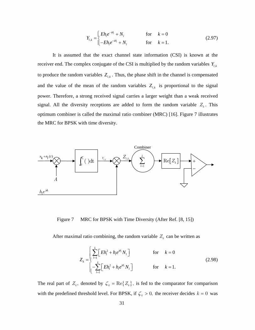
optimum combiner is called the maximal ratio combiner (MRC) [16]. Figure 7 illustrates

the MRC for BPSK with time diversity.

Figure 7 MRC for BPSK with Time Diversity (After Ref. [8, 15])

After maximal ratio combining, the random variable kZ can be written as

2

1

2

1

for 0

for 1.

θ

θ

=

=

⎧ ⎡ ⎤+ =⎪ ⎣ ⎦⎪= ⎨⎪ ⎡ ⎤− + =⎣ ⎦⎪⎩

∑

∑

l

l

Li

l l ll

k Li

l l ll

Eh h e N kZ

Eh h e N k (2.98)

The real part of ,kZ denoted by { }ζ = Re ,k kZ is fed to the comparator for comparison

with the predefined threshold level. For BPSK, if 0,kζ > the receiver decides 0k = was

( )+x n tk l

−

0( )dtcT

∫

A

,l kZ,l kY

1

L

l=∑

ljlhe

φ

Combiner

+ [ ]Re kZ

32

transmitted. If 0,kζ < the receiver decides 1k = was transmitted. The decision variable

kζ can be written as

[ ]( )

( )

2

1

2

1

Re for 0Re

Re for 1.

θ

θ

ζ =

=

⎧ ⎡ ⎤+ =⎪ ⎣ ⎦⎪= = ⎨⎪ ⎡ ⎤− + =⎣ ⎦⎪⎩

∑

∑

l

l

Li

l l ll

k k Li

l l ll

Eh h e N kZ

Eh h e N k (2.99)

From Equation (2.99), it is evident that the decision variable kζ is a Gaussian random

variable with conditional mean (conditioned on the value of =∑ 2

1

L

ll

h )

2

1

( 1) .L

kk l

l

E hζ=

= − ∑ (2.100)

Since the lN ’s are independent zero-mean complex Gaussian random variables with

circularly symmetric probability density function and variance equal to 0EN , the

conditional variance of kζ can be expressed as:

( ){ }

( ){ }

{ }

0 1

2 2 2

1

2

1

2

1

20

1

Var Re

Var Re

1 Var2

2

ζ ζ ζ

ϕ

σ σ σ

=

=

=

=

= =

=

=

=

=

∑

∑

∑

∑

l

Li

l llL

l ll

L

l ll

L

ll

h e N

h N

h N

EN h

. (2.101)

Assuming the probability of transmitting a “1” bit and a “0” bit are equal and using the

fact that the conditional probabilities of bit error |b kP are equal due to the symmetry of the

noise probability density function and the zero threshold, it is possible to calculate the

conditional probability of bit error as:

33

{ }|0 |1 |0 0

0 0 0

0 0 0

0

2

10

1 1 Pr 02 2

Pr

Pr

2 .

ζ ζ

ζ ζ

ζ

ζ

ζ ζ ζσ σ

ζ ζ ζσ σ

ζσ

=

= + = = <

⎧ ⎫−⎪ ⎪= < −⎨ ⎬⎪ ⎪⎩ ⎭⎧ ⎫−⎪ ⎪= >⎨ ⎬⎪ ⎪⎩ ⎭⎛ ⎞

= ⎜ ⎟⎜ ⎟⎝ ⎠⎛ ⎞

= ⎜ ⎟⎜ ⎟⎝ ⎠

∑

b b b b

L

ll

P P P P

Q

EQ hN

(2.102)

Where ( )Q x is defined as [18]

( )2

212π

∞ −= ∫

u

xQ x e du . (2.103)

Let γ be defined as

2

10

γ=

= ∑L

ll

E hN

. (2.104)

Substituting Equation (2.103) into (2.102), it is possible to rewrite the conditional

probability of bit error as a probability of bit error conditioned on γ :

( )( ) 2 .γ γ=bP Q (2.105)

The average probability of bit error can be obtained by taking the expectation of ( )γbP

with respect to random variable γ [15, 16]. The average probability of bit error can be

written as

( )

( ) ( )

E γ

γ γ γ∞

Γ−∞

= ⎡ ⎤⎣ ⎦

= ∫b b

b

P P

P f d (2.106)

where ( )f γΓ is the probability density function for γ . Similarly, γ l can be written as

34

2

0

.γ = ll

EhN

(2.107)

The probability distribution function of 2lh was derived in the last section. Taking 2

l lh v= ,

Equation (2.60) can be represented as

( ) ( )2/ 22

1 .2

σ

σ−= l

l

vV l lf v e u v (2.108)

The average SNR per diversity reception can be written as

[ ]

[ ]

2

0

2

0 0

=E =E

= E = E

γ γ⎡ ⎤⎢ ⎥⎣ ⎦

⎡ ⎤⎣ ⎦

ll l

l l

EhN

E Eh vN N

. (2.109)

The expectation can be evaluated as

[ ]

2

0

/ 2 22

0

E ( )

1 = 2 .2

l

l

l l V l l

vl l

v v f v dv

v e dvσ σσ

∞

∞−

=

=

∫

∫ (2.110)

Now the Equation (2.109) can be written as

2

0

2 σγ =lEN

. (2.111)

The characteristic function of lV can be written as [8, 16]

( ) ( )2

11 2

ωσ ω

=−lVF

i. (2.112)

If L IID random variables are added, then the probability density function of the sum is

the L -fold convolution of the probability density function of the single random variable.

Therefore, the characteristic function of the sum is the characteristic function of the

single random variable raised to the power of L [16, 18]. Therefore, the characteristic

function for 1

L

ll

V V=

= ∑ is

35

( )( )2

1 .1 2

ωσ ω

=−

V LFi

(2.113)

The probability density function of V is the inverse Fourier transform of the

characteristic function and can be written as [8]

( ) 21

/ 22 ( )

2 ( 1)!

Lv

V L L

vf v e u vL

σ

σ

−−=

−. (2.114)

Consistent with Equation (2.104), it is possible to write

0

γ = EvN

(2.115)

and

γ=

o

d Edv N

. (2.116)

Now, the probability distribution function for γ can be given as

( ) ( )

( )( )

2

2

1/ 2

2

0

21

2

0

12 1 !

2 1 !

o

o

Lv

L L

v EN

ELN

L

vf eE LN

f eE L

N

σ

γ

γσ

γσ

γγσ

−−

Γ

=

−−

Γ

=−

=⎛ ⎞

−⎜ ⎟⎝ ⎠

. (2.117)


( )( ) ( )

( )1

1 !

γγγγ γ

γ

− −

Γ =−

l

L

Lf e uL

. (2.118)

Now, substituting Equation (2.105) and (2.118) into Equation (2.106), the average

probability of bit error can be represented as [8]

36

( ) ( ) ( )

1

02

1 !

γγγγ γ

γ

− −∞=

−∫ l

L

b Ll

P Q e dL

. (2.119)

The solution for Equation (2.119) has been given in [16] as

( ) ( )1

0

11 12 2

−

=

− +− +⎡ ⎤ ⎡ ⎤⎛ ⎞= ⎢ ⎥ ⎢ ⎥⎜ ⎟

⎝ ⎠⎣ ⎦ ⎣ ⎦∑

L lL

bl

L lu uP

l (2.120)

where u is defined as

1γγ

=+

u . (2.121)

In time diversity, the total bit energy received is proportional to the number of diversity

receptions and is represented as

bE LE= (2.122)

where L is the number of diversity reception and E is the energy per diversity reception.

Substituting Equation (2.122) into Equation (2.109), γ l can be written as

22 σγ = b

lo

ELN

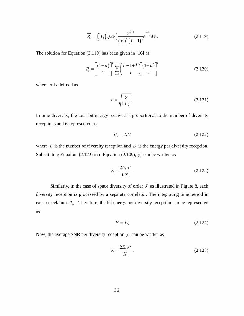
. (2.123)

Similarly, in the case of space diversity of order J as illustrated in Figure 8, each

diversity reception is processed by a separate correlator. The integrating time period in

each correlator is bT . Therefore, the bit energy per diversity reception can be represented

as

bE E= (2.124)

Now, the average SNR per diversity reception γ l can be written as

2

0

2 σγ = bl

EN

. (2.125)

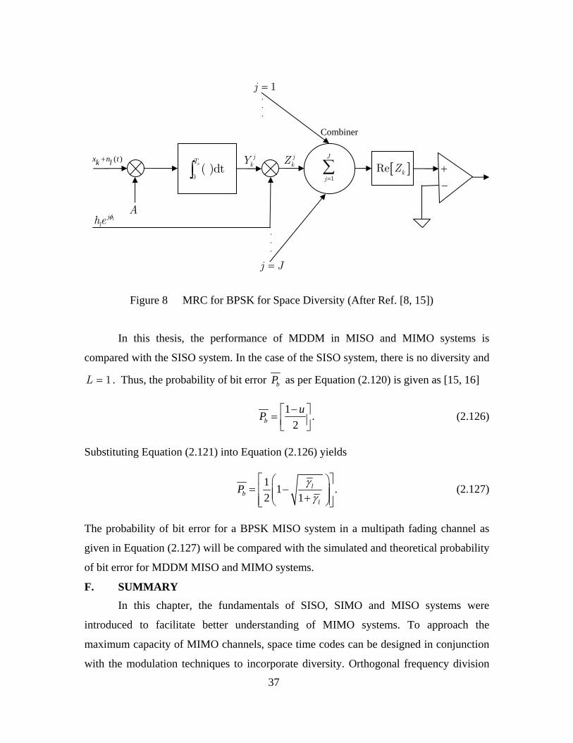
37

Figure 8 MRC for BPSK for Space Diversity (After Ref. [8, 15])

In this thesis, the performance of MDDM in MISO and MIMO systems is

compared with the SISO system. In the case of the SISO system, there is no diversity and

1L = . Thus, the probability of bit error bP as per Equation (2.120) is given as [15, 16]

1 .2−⎡ ⎤= ⎢ ⎥⎣ ⎦

buP (2.126)


1 1 .2 1

γγ

⎡ ⎤⎛ ⎞= −⎢ ⎥⎜ ⎟⎜ ⎟+⎢ ⎥⎝ ⎠⎣ ⎦

lb

l

P (2.127)

The probability of bit error for a BPSK MISO system in a multipath fading channel as

given in Equation (2.127) will be compared with the simulated and theoretical probability

of bit error for MDDM MISO and MIMO systems.

F. SUMMARY In this chapter, the fundamentals of SISO, SIMO and MISO systems were

introduced to facilitate better understanding of MIMO systems. To approach the

maximum capacity of MIMO channels, space time codes can be designed in conjunction

with the modulation techniques to incorporate diversity. Orthogonal frequency division

( )+x n tk l

ljlhe

φ

−

0( )dtsT

∫

A

jkZ

jkY

1

J

j=∑

Combiner

+ [ ]Re kZ

1j =

j J=

.

.

.

.

.

.

38

multiplexing (OFDM) can be used to mitigate the frequency selectivity of the channel.

OFDM utilizes the discrete Fourier transform (DFT) of the baseband signal. The

multicarrier cyclic delay diversity technique can be implemented by exploiting the cyclic

shift property of the DFT. A baseband model for the flat Rayleigh fading channel was

derived for simulation. Lastly, the MRC as an optimum diversity combining technique

was discussed. The next chapter discusses the design of the simulated MDDM

transmitters and receivers.

39

III. MULTICARRIER DELAY DIVERSITY MODULATION TRANSMITTER AND RECEIVER MODELS

This chapter introduces the implementation of the multicarrier delay diversity

modulation scheme at the block level. The basic design of the transmitter and receiver is

discussed briefly. In this thesis, the MDDM scheme is implemented using BPSK

modulation. The inclusion of forward error correction (FEC) and higher bandwidth

efficient modulation schemes can be considered for future work. The next chapter

illustrates the simulation and analysis of the MDDM transmitter and receiver.

A. THE MULTICARRIER DELAY DIVERSITY MODULATION SCHEME The scheme of implementing delay diversity with OFDM for MIMO systems was

recommended for flat fading channels in [5]. The cyclic delay diversity approach with

OFDM was suggested for the frequency selective fading channel in [6]. In this research,

cyclic delay diversity with OFDM is investigated. The implementation of multicarrier

delay diversity in MIMO systems has been discussed in the previous chapter. For

modeling purposes, the MIMO configuration of two transmit and two receive antennas is

discussed in this chapter. For simulation and analysis, the number of receive antennas

varies from one to three. To facilitate better understanding and precise representation of

signals from the transmit antenna to the receive antenna, the following notations will be

used:

• kX represents the BPSK symbol at k -th interval before the multicarrier delay diversity modulation and after demodulation

• lkX represents the BPSK symbol at k -th interval from the transmitting

antenna l after multicarrier delay diversity delay modulation

• lmx represents the signal x to be transmitted from transmit antenna l in

the -thm transmission interval,

• jmr represents the received signal at receive antenna j at the -thm time

interval,

• ljh represents the channel response from transmit antenna l to receive antenna j ,

• jn represents the AWGN at receive antenna j , and

• asterisk ( )∗ represents the complex conjugate.

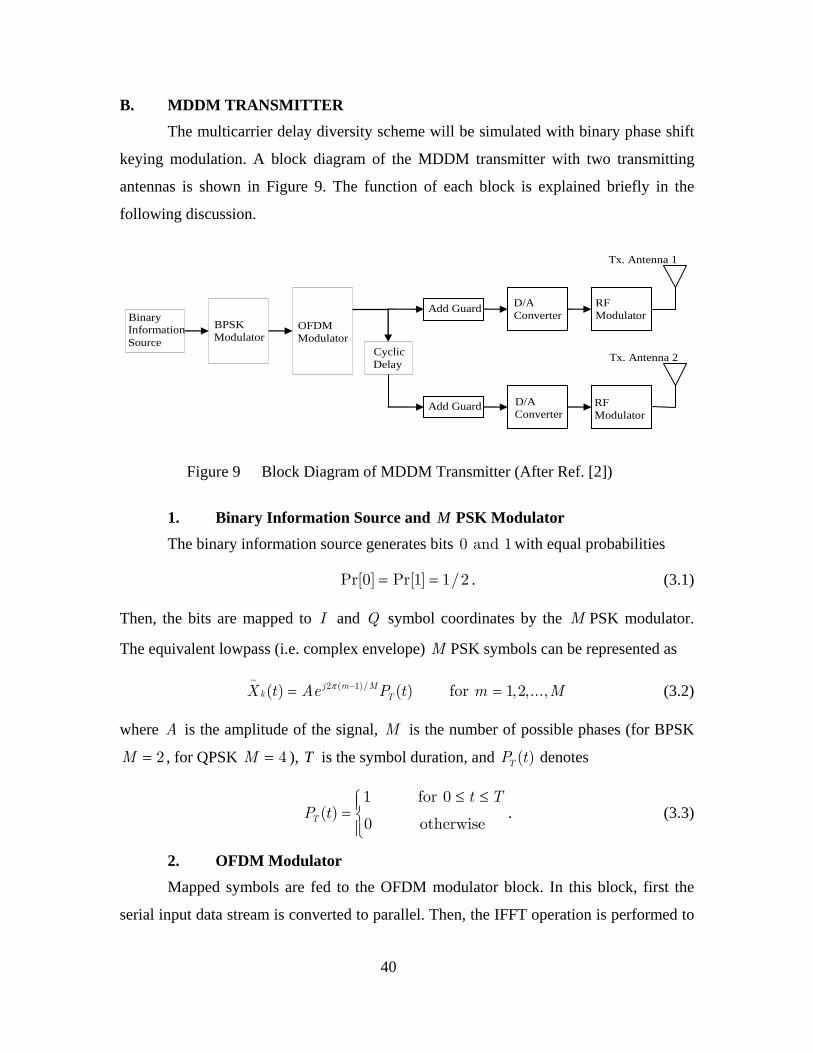
40

B. MDDM TRANSMITTER The multicarrier delay diversity scheme will be simulated with binary phase shift

keying modulation. A block diagram of the MDDM transmitter with two transmitting

antennas is shown in Figure 9. The function of each block is explained briefly in the

following discussion.

Binary Information Source

BPSK Modulator

OFDM Modulator

Cyclic Delay

Add Guard D/A Converter

D/A Converter

RF Modulator

Add Guard RF Modulator

Tx. Antenna 2

Tx. Antenna 1

Figure 9 Block Diagram of MDDM Transmitter (After Ref. [2])

1. Binary Information Source and M PSK Modulator The binary information source generates bits 0 and 1 with equal probabilities

Pr[0] Pr[1] 1/2= = . (3.1)

Then, the bits are mapped to I and Q symbol coordinates by the M PSK modulator.

The equivalent lowpass (i.e. complex envelope) M PSK symbols can be represented as

π −= =∼

2 ( 1)/( ) ( ) for 1,2,...,j m Mk TX t Ae P t m M (3.2)

where A is the amplitude of the signal, M is the number of possible phases (for BPSK

2M = , for QPSK 4M = ), T is the symbol duration, and ( )TP t denotes

≤ ≤⎧⎪= ⎨

⎪⎩

1 for 0( )

0 otherwiseT

t TP t . (3.3)

2. OFDM Modulator Mapped symbols are fed to the OFDM modulator block. In this block, first the

serial input data stream is converted to parallel. Then, the IFFT operation is performed to

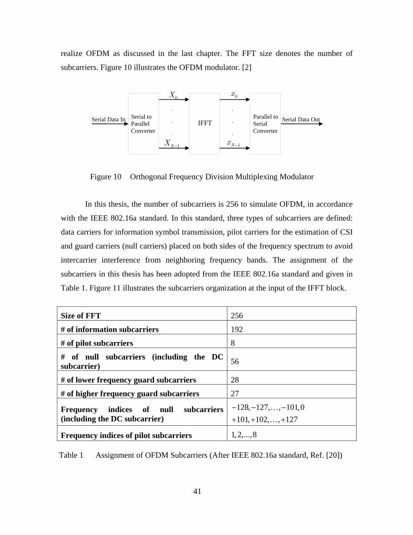
41

realize OFDM as discussed in the last chapter. The FFT size denotes the number of

subcarriers. Figure 10 illustrates the OFDM modulator. [2]

Figure 10 Orthogonal Frequency Division Multiplexing Modulator

In this thesis, the number of subcarriers is 256 to simulate OFDM, in accordance

with the IEEE 802.16a standard. In this standard, three types of subcarriers are defined:

data carriers for information symbol transmission, pilot carriers for the estimation of CSI

and guard carriers (null carriers) placed on both sides of the frequency spectrum to avoid

intercarrier interference from neighboring frequency bands. The assignment of the

subcarriers in this thesis has been adopted from the IEEE 802.16a standard and given in

Table 1. Figure 11 illustrates the subcarriers organization at the input of the IFFT block.

Size of FFT 256

# of information subcarriers 192

# of pilot subcarriers 8

# of null subcarriers (including the DC subcarrier) 56

# of lower frequency guard subcarriers 28

# of higher frequency guard subcarriers 27

Frequency indices of null subcarriers (including the DC subcarrier)

128, 127, , 101,0101, 102, , 127

− − −+ + +

……

Frequency indices of pilot subcarriers 1,2,...,8 Table 1 Assignment of OFDM Subcarriers (After IEEE 802.16a standard, Ref. [20])

Serial to Parallel Converter

Serial Data In IFFT

.

.

.

0X

1NX −

.

.

.

0x

1Nx −

Parallel to Serial Converter

Serial Data Out

42

+127

+101

-101

- 128

IFFT0

-100

-60

-36

-1

+9

+36

+60

+100

192 information symbols

27 null subcarriers

28 null subcarriers

8 pilot subcarriers

DC subcarrier

Figure 11 Assignment of Subcarriers at the Input of IFFT Block (After Ref. [20])

The output of the IFFT block can be represented according to the definition of Equation

(2.30) as

π−

=

= =∑1

2 /

0

1 for m 0,1,2,...,255

Nj km N

m kk

x X eN

(3.4)

where 256,N = and the index of the subcarrier is represented from 0 to 255 instead of

128− to 128 for convenience. After the IFFT operation, the OFDM sequence is

converted from parallel to serial. [23]

3. Cyclic Delay Addition

After the IFFT operation, the symbols nx are cyclically shifted to realize a cyclic

delay of one information symbol period. For transmitting antenna 1 , there is no delay and

0.D = For each subsequent antenna, the cyclic delay is increased one information

symbol period. The signal after cyclic delay is given as

−= = = −( ) where 1,2,..., and 1N

ln n Dx x l L D l (3.5)

4. Guard Interval (Cyclic Prefix) Addition As discussed in the previous chapter, a guard interval at the beginning of each

OFDM symbol is added to mitigate the effect of the multipath channel. The length of the

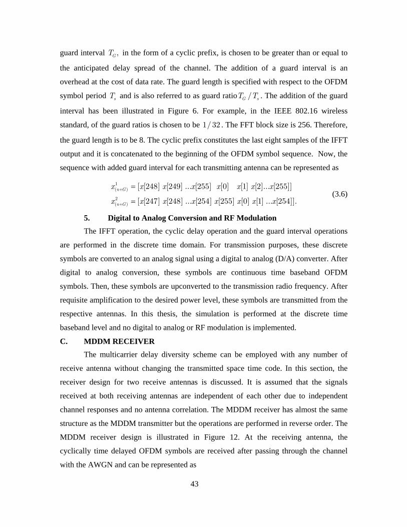
43

guard interval ,GT in the form of a cyclic prefix, is chosen to be greater than or equal to

the anticipated delay spread of the channel. The addition of a guard interval is an

overhead at the cost of data rate. The guard length is specified with respect to the OFDM

symbol period sT and is also referred to as guard ratio /G sT T . The addition of the guard

interval has been illustrated in Figure 6. For example, in the IEEE 802.16 wireless

standard, of the guard ratios is chosen to be 1/32 . The FFT block size is 256. Therefore,

the guard length is to be 8. The cyclic prefix constitutes the last eight samples of the IFFT

output and it is concatenated to the beginning of the OFDM symbol sequence. Now, the

sequence with added guard interval for each transmitting antenna can be represented as

+

+

=

=

1( )

2( )

[ [248] [249] ... [255] [0] [1] [2]... [255]]

[ [247] [248] ... [254] [255] [0] [1] ... [254]].

n G

n G

x x x x x x x x

x x x x x x x x (3.6)

5. Digital to Analog Conversion and RF Modulation The IFFT operation, the cyclic delay operation and the guard interval operations

are performed in the discrete time domain. For transmission purposes, these discrete

symbols are converted to an analog signal using a digital to analog (D/A) converter. After

digital to analog conversion, these symbols are continuous time baseband OFDM

symbols. Then, these symbols are upconverted to the transmission radio frequency. After

requisite amplification to the desired power level, these symbols are transmitted from the

respective antennas. In this thesis, the simulation is performed at the discrete time

baseband level and no digital to analog or RF modulation is implemented.

C. MDDM RECEIVER The multicarrier delay diversity scheme can be employed with any number of

receive antenna without changing the transmitted space time code. In this section, the

receiver design for two receive antennas is discussed. It is assumed that the signals

received at both receiving antennas are independent of each other due to independent

channel responses and no antenna correlation. The MDDM receiver has almost the same

structure as the MDDM transmitter but the operations are performed in reverse order. The

MDDM receiver design is illustrated in Figure 12. At the receiving antenna, the

cyclically time delayed OFDM symbols are received after passing through the channel

with the AWGN and can be represented as

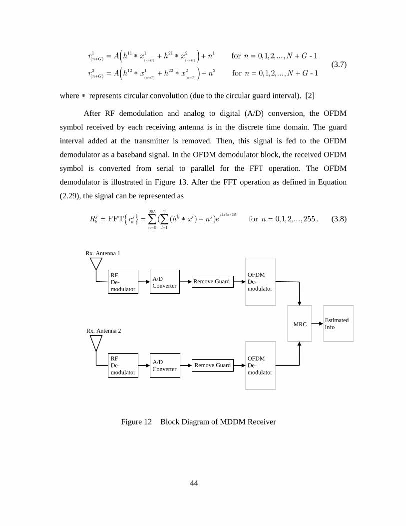
44

( )( )

+ +

+ +

+

+

= ∗ + ∗ + = +

= ∗ + ∗ + = +

( ) ( )

( ) ( )

1 11 1 21 2 1( )

2 12 1 22 2 2( )

for 0,1,2,..., - 1

for 0,1,2,..., - 1

n G n G

n G n G

n G

n G

r A h x h x n n N G

r A h x h x n n N G (3.7)

where ∗ represents circular convolution (due to the circular guard interval). [2]

After RF demodulation and analog to digital (A/D) conversion, the OFDM

symbol received by each receiving antenna is in the discrete time domain. The guard

interval added at the transmitter is removed. Then, this signal is fed to the OFDM

demodulator as a baseband signal. In the OFDM demodulator block, the received OFDM

symbol is converted from serial to parallel for the FFT operation. The OFDM

demodulator is illustrated in Figure 13. After the FFT operation as defined in Equation

(2.29), the signal can be represented as

{ } π

= =

= = ∗ + =∑ ∑2 /255

255 2

0 1

FFT ( ( ) ) for 0,1,2,...,255j knj j lj l j

k nn l

R r h x n e n . (3.8)

Estimated Info MRC

Remove Guard A/D Converter

A/D Converter

RF De-modulator

Rx. Antenna 2

OFDM De-modulator

OFDM De- modulator

Remove Guard

RF De-modulator

Rx. Antenna 1

Figure 12 Block Diagram of MDDM Receiver

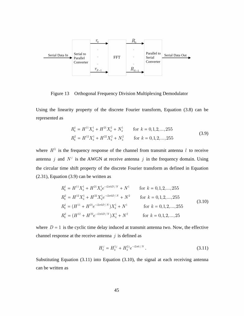
45

Figure 13 Orthogonal Frequency Division Multiplexing Demodulator

Using the linearity property of the discrete Fourier transform, Equation (3.8) can be

represented as

= + + =

= + + =

1 11 1 21 2 1

2 12 1 22 2 2

for 0,1,2,...,255

for 0,1,2,...,255

k k k k

k k k k

R H X H X N k

R H X H X N k (3.9)

where ljH is the frequency response of the channel from transmit antenna l to receive

antenna j and jN is the AWGN at receive antenna j in the frequency domain. Using

the circular time shift property of the discrete Fourier transform as defined in Equation

(2.31), Equation (3.9) can be written as

π

π

π

π

−

−

−

−

= + + =

= + + =

= + + =

= + +

1 11 1 21 1 2 / 1

2 12 1 22 1 2 / 2

1 11 21 2 / 1 1

2 12 22 2 / 1 2

for 0,1,2,...,255

for 0,1,2,...,255

( ) for 0,1,2,...,255

( )

i kD Nk k k

i kD Nk k k

i kD Nk k

i kD Nk k

R H X H X e N k

R H X H X e N k

R H H e X N k

R H H e X N = for 0,1,2,...,25k

(3.10)

where 1D = is the cyclic time delay induced at transmit antenna two. Now, the effective

channel response at the receive antenna j is defined as

1 2 2 /j j j i k Nk k kH H H e π−= + . (3.11)

Substituting Equation (3.11) into Equation (3.10), the signal at each receiving antenna

can be written as

Serial to Parallel Converter

Serial Data In FFT .

.

.

0r

1Nr −

.

.

.

0R

1NR −

Parallel to Serial Converter

Serial Data Out

46

= +

= +

1 1 1 1

2 2 1 2

k k k k

k k k k

R H X N

R H X N. (3.12)

Equation (3.12) shows clearly the space diversity receptions at the receiving end.

They are combined by using the optimum maximal ratio combining receiver. MRC for

space diversity has already been discussed in the previous chapter and illustrated in

Figure 8. It is assumed that perfect CSI is known at the receiver end. In MRC, the

received signal is multiplied with the complex conjugate of CSI and all diversity

receptions are added to form the decision variable. The outputs of the integrators of the

MRC for each diversity reception can be represented as

= +

= +

= +

= +

1 1 1'

2 2 2 '

11 1'

22 2 '

k b k k k

k b k k k

b k kk k

b k kk k

Y ATH X N

Y ATH X N

E H XY N

AE H X

Y NA

(3.13)

where bE is the average energy per bit, =1' 1k b kN ATN , and =2 ' 2

k b kN ATN .

After the integrator stage, the random variable is multiplied by the complex

conjugate of CSI and the resulting random variable can be represented as

∗∗

∗∗

∗

∗

= +

= +

= +

= +

1 11 1 1'

2 22 2 2 '

211 1 1'

222 2 2 '

( )( )

( )( )

( )

( )

b k k kk k k

b k k kk k k

b k kk k k

b k kk k k

E H H XZ H N

AE H H X

Z H NA

E H XZ H N

A

E H XZ H N

A

. (3.14)

The decision variable kZ at the output of combiner stage can be expressed as

( ) ∗ ∗

= +

= + + +

1 2

2 21 2 1 '1 2 '2( ) ( )

k k k

kk b k k k k

Z Z Z

XZ E H H H N H N

A

. (3.15)

47

For the final decision of the estimated received data, the decision variable is

compared with predetermined threshold levels. For the case of BPSK, the real part of kZ

is compared with a threshold level of zero to decide each received binary bit. [2, 15]

D. SUMMARY This chapter discussed the designs of the MDDM transmitter and receiver at the

block level. The function of each block was discussed with the representation of signals

before and after each block operation. During the discussion, two assumptions were

made, i.e., perfect knowledge of CSI at the receiver and constant channel response for the

duration of the OFDM symbol. The next chapter analyzes the MDDM transmitter and

receiver model for the AWGN channel with and without flat fading.

48


49

IV. ANALYSIS AND SIMULATION OF MULTICARRIER DELAY DIVERSITY MODULATION SCHEME

In this chapter, the performance (bit error probability) analysis and simulation of

MISO and MIMO systems with multicarrier delay diversity is presented. The MDDM

transmitter and receiver as described in Chapter III were simulated in Matlab. The system

is analyzed with an AWGN channel with and without Rayleigh fading. The analytical

and simulated results are compared with a SISO BPSK system. To establish a fair

comparison of the SISO system and the MIMO system with MDDM, the power

transmitted for both systems is assumed equal. To facilitate better understanding and

precise representation of signals from transmit to receive antenna, this thesis will adhere

to the following notation:

• bE represents the average energy per bit at the receiver of the SISO system,

• '

sE represents the average energy per MIMO BPSK symbol per receiving antenna,

• sT represents the OFDM symbol duration,

• 'sT represents the MIMO BPSK symbol duration and '

s bT T=

• ζ k represents the real part of decision variable kZ .

Energy per bit is an important parameter for comparison and is defined as

2

2

0

bT

b k bE X dt AT= =∫ (4.1)

where k is the time index of the BPSK symbol (before serial to parallel and after

parallel to serial conversions) and kX is the BPSK modulated symbol as defined in Table

2.

Input bit at time k Output Symbol kX

0 A

1 A−

Table 2 BPSK Modulation Scheme (After Ref. [8])

50

For simulation and analysis, the amplitude 1A = is maintained. Equation (4.1)

shows that the energy per bit for BPSK modulation is the same for bit 0 and bit 1 . Thus

the transmitted power for the SISO system can be written as

2bSISO

b

EP A

T= = (4.2)

The probability of bit error bP for a baseband equivalent SISO BPSK system in

discrete domain for correlation demodulator can be represented as [15, 16]

bZ

ZP Q

σ

−+⎛ ⎞

⎜ ⎟=⎜ ⎟⎝ ⎠

. (4.3)

In this case Z−+ is represented as

Z A−+ = (4.4)

and

2 0

2Zb

NT

σ = (4.5)

where 0

2N represents the two sided noise power spectral density for the real part of the

AWGN. Substituting Equation (4.4) and Equation (4.5) into Equation (4.3) yields,

2 2b bb

o o

T A EP Q Q

N N

⎛ ⎞ ⎛ ⎞= =⎜ ⎟ ⎜ ⎟⎜ ⎟ ⎜ ⎟

⎝ ⎠ ⎝ ⎠. (4.6)

The bit error probability of the SISO system as given by Equation (4.6) will serve as a

benchmark for comparison of the MISO and MIMO systems with MDDM in the AWGN

channel.

In this thesis the number of transmit antennas is two and both the transmit

antennas transmit equal power. The total energy per bit transmitted for MISO and MIMO

systems using BPSK symbols can be defined as

' ' 's sE PT= (4.7)

51

and

SISO MISO MIMOP P P= = . (4.8)

Therefore, the energy transmitted per antenna 'P can be given as

'

2SISO SISOP P

PL

= = . (4.9)

Now, Equation (4.7) is rewritten as

'' ' '

'

2

.2

SISO ss s

bs

P TE PT

EE

= =

= (4.10)

A. SIMULATION OF MDDM TRANSMITTER The block diagram of the MDDM transmitter model is shown in Figure 9. The

MDDM transmitter was simulated in MATLAB with equivalent baseband BPSK in the

discrete time domain. The simulation was implemented with one sample for each BPSK

symbol. The MDDM transmitter scheme, as mentioned in Chapter III with two

transmitting antennas, was simulated without added guard interval, D/A converter and RF

modulator blocks to facilitate the simulations. Equal power was transmitted from both the

antennas. To achieve the same total power transmission as that of a single antenna BPSK

transmitter, the signal at each branch of MIMO transmitter was multiplied with a gain

factor of g for normalization. The transmitted energy per symbol for BPSK is same

whether a binary 1 or 0 is transmitted. With the gain factor g the energy per symbol is

represented as

' 2

' 2 2 '

0

sT

s k sE gX dt g AT= =∫ . (4.11)


'

2 2 '

2SISO s

s

P Tg AT= . (4.12)

Using Equation (4.2), Equation (4.12) can be rewritten as

52

2 121

.2

g

g

=

= (4.13)

The gain factor 1/ 2g = is maintained for all subsequent simulations to transmit the

same power as that of a single antenna BPSK system. Thus the effective amplitude of the

BPSK modulated signal for each antenna is given as

= =1

2 2k

AX . (4.14)

B. SIMULATION OF MDDM RECIVER The block diagram of the MDDM receiver model is shown in Figure 12. The

MDDM receiver was also simulated in MATLAB with equivalent baseband BPSK in the

discrete time domain. The MDDM receiver simulation was implemented as discussed in

Chapter III except for the RF demodulator, the A/D converter and the Remove Guard

blocks. The receiver was configured as a MISO system with only one receive antenna

and as a MIMO system with two receive antennas and as a MIMO system with three

receive antennas. After multicarrier delay diversity demodulation, the space diversity

receptions of MIMO systems were combined by using the optimum MRC technique as

discussed in Chapter II. After the BPSK correlation demodulator as illustrated in Figure

14, ζ k (the real part of the random variable kZ ) was compared with the threshold level

according to Table 3. For analysis and simulation purposes it is assumed that the

transmitter and receiver frequencies are synchronized and, in the case of MIMO systems,

all the diversity receptions are also synchronized.

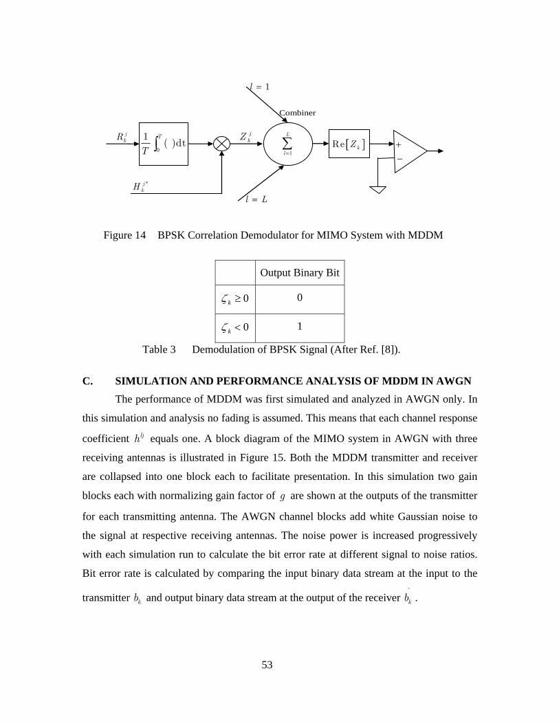
53

− 0

1( )dt

T

T ∫ jkZ

1

L

l =∑

Combiner

+ [ ]Re kZ

1l =

l L=

jkR

*jkH

Figure 14 BPSK Correlation Demodulator for MIMO System with MDDM

Output Binary Bit

0kζ ≥ 0

0kζ < 1

Table 3 Demodulation of BPSK Signal (After Ref. [8]).

C. SIMULATION AND PERFORMANCE ANALYSIS OF MDDM IN AWGN

The performance of MDDM was first simulated and analyzed in AWGN only. In

this simulation and analysis no fading is assumed. This means that each channel response

coefficient ljh equals one. A block diagram of the MIMO system in AWGN with three

receiving antennas is illustrated in Figure 15. Both the MDDM transmitter and receiver

are collapsed into one block each to facilitate presentation. In this simulation two gain

blocks each with normalizing gain factor of g are shown at the outputs of the transmitter

for each transmitting antenna. The AWGN channel blocks add white Gaussian noise to

the signal at respective receiving antennas. The noise power is increased progressively

with each simulation run to calculate the bit error rate at different signal to noise ratios.

Bit error rate is calculated by comparing the input binary data stream at the input to the

transmitter kb and output binary data stream at the output of the receiver ^

kb .

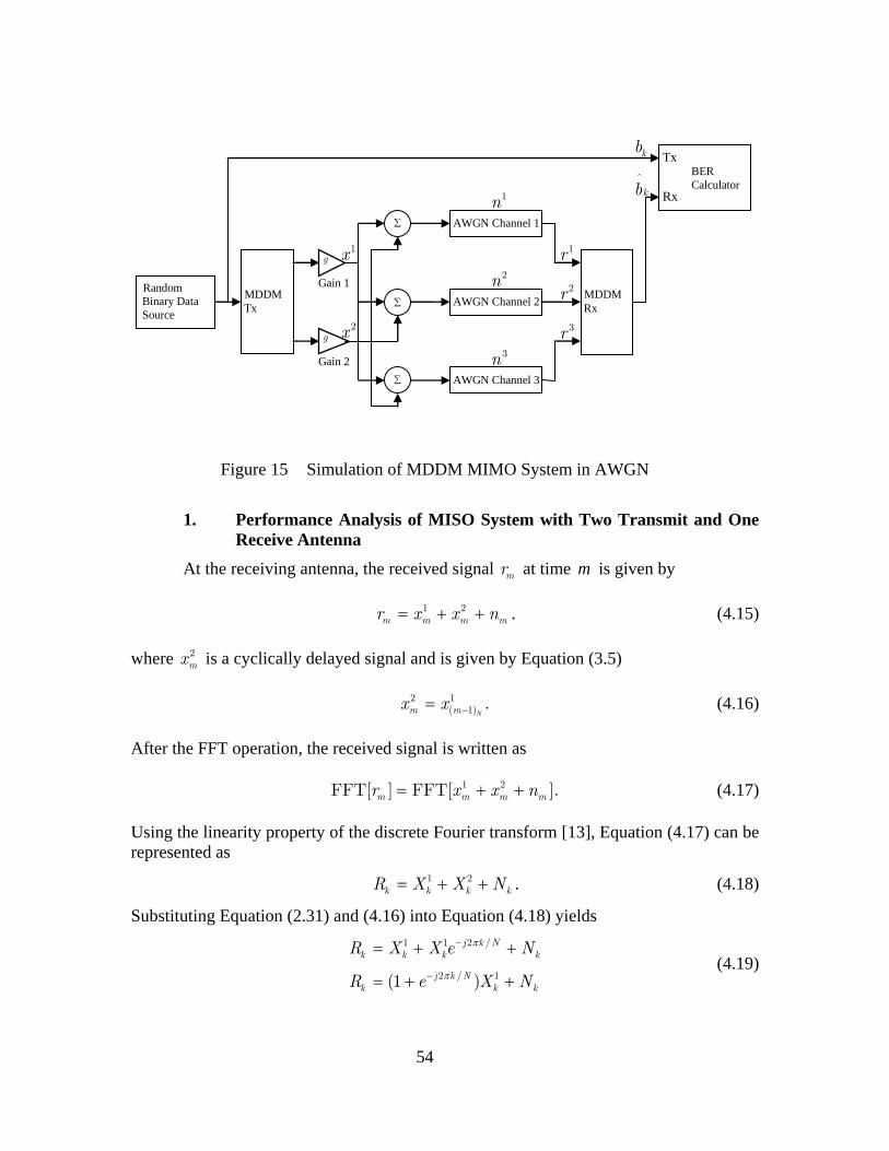
54

Random Binary Data Source

MDDM Tx

AWGN Channel 1

g

∑

g

∑

∑

AWGN Channel 3

AWGN Channel 2 MDDM Rx

BER Calculator

Tx

Rx 1n

2n

3n

Gain 1

Gain 2

1r

2r

3r 2x

1x

kb

^

kb

Figure 15 Simulation of MDDM MIMO System in AWGN

1. Performance Analysis of MISO System with Two Transmit and One

Receive Antenna

At the receiving antenna, the received signal mr at time m is given by

1 2m m m mr x x n= + + . (4.15)

where 2mx is a cyclically delayed signal and is given by Equation (3.5)

2 1( 1) .

Nm mx x −= (4.16)

After the FFT operation, the received signal is written as

= + +1 2FFT[ ] FFT[ ].m m m mr x x n (4.17)

Using the linearity property of the discrete Fourier transform [13], Equation (4.17) can be represented as

= + +1 2k k k kR X X N . (4.18)

Substituting Equation (2.31) and (4.16) into Equation (4.18) yields

π

π

−

−

= + +

= + +

1 1 2 /

2 / 1(1 )

j k Nk k k k

j k Nk k k

R X X e N

R e X N (4.19)

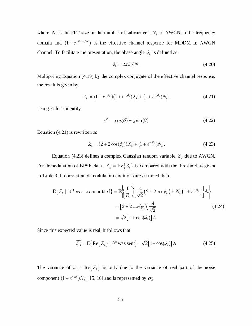
55

where N is the FFT size or the number of subcarriers, kN is AWGN in the frequency

domain and 2 /(1 )j k Ne π−+ is the effective channel response for MDDM in AWGN

channel. To facilitate the presentation, the phase angle kφ is defined as

2 / .k k Nφ π= (4.20)

Multiplying Equation (4.19) by the complex conjugate of the effective channel response,

the result is given by

φ φ φ− + += + + + +1(1 )(1 ) (1 )k k kj j jk k kZ e e X e N . (4.21)

Using Euler’s identity

cos( ) sin( )je jθ θ θ= + (4.22)

Equation (4.21) is rewritten as

φφ += + + +1(2 2 cos( )) (1 )kjk k k kZ X e N . (4.23)

Equation (4.23) defines a complex Gaussian random variable kZ due to AWGN.

For demodulation of BPSK data , { }ζ = Rek kZ is compared with the threshold as given

in Table 3. If correlation demodulator conditions are assumed then

{ } ( ) ( )

[ ]

[ ]

φφ

φ

φ

+⎧ ⎫⎪ ⎪⎡ ⎤= + + +⎨ ⎬⎢ ⎥⎣ ⎦⎪ ⎪⎩ ⎭

= +

= +

∫0

1E | " 0" was transmitted E 2 2cos 1

2

2 2 cos( )2

2 1 cos( ) .

b

k

Tj

k k kb

k

k

AZ N e dt

T

A

A

(4.24)

Since this expected value is real, it follows that

{ }{ } [ ]E Re | "0" was sent 2 1 cos( )k k kZ Aζ φ+= = + (4.25)

The variance of { }ζ = Rek kZ is only due to the variance of real part of the noise

component φ++(1 )kj ke N [15, 16] and is represented by ζσ2

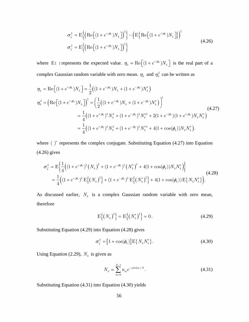
56

( ){ } { }( )( ){ }

φ φζ

φζ

σ

σ

+ +

+

⎡ ⎤ ⎡ ⎤= + − +⎣ ⎦ ⎣ ⎦

⎡ ⎤= +⎣ ⎦

222

22

E Re (1 ) E Re (1 )

E Re (1 )

k k

k

j jk k

jk

e N e N

e N (4.26)

where { }E represents the expected value. Re (1 )kjk ke Nφη +⎡ ⎤= +⎣ ⎦ is the real part of a

complex Gaussian random variable with zero mean. kη and 2kη can be written as

( )

( ) ( )

( )

φ φ φ

φ φ φ

φ φ φ φ

η

η

+ + − ∗

+ + − ∗

+ − ∗ − + ∗

⎡ ⎤= + = + + +⎣ ⎦

⎛ ⎞⎡ ⎤= + = + + +⎜ ⎟⎣ ⎦ ⎝ ⎠

= + + + + + +

222

2 2 2 2

1Re (1 ) (1 ) (1 )

21

Re (1 ) (1 ) (1 )2

1 (1 ) (1 ) 2(1 )(1 )

4

k k k

k k k

k k k k

j j jk k k k

j j jk k k k

j j j jk k k k

e N e N e N

e N e N e N

e N e N e e N N

( )φ φ φ+ − ∗ ∗= + + + + +2 2 2 21 (1 ) (1 ) 4(1 cos( )) .

4k kj j

k k k k ke N e N N N

(4.27)

where ( )∗ represents the complex conjugate. Substituting Equation (4.27) into Equation

(4.26) gives

( ) ( )( ){ }( ){ } ( ){ } { }( )

φ φζ

φ φ

σ φ

φ

+ − ∗ ∗

+ − ∗ ∗

= + + + + +

= + + + + +

222 2 2

222 2

1E (1 ) (1 ) 4(1 cos( ))

41

(1 ) E (1 ) E 4(1 cos( ))E .4

k k

k k

j jk k k k k

j jk k k k k

e N e N N N

e N e N N N(4.28)

As discussed earlier, kN is a complex Gaussian random variable with zero mean,

therefore

( ){ } ( ){ }∗= =22E E 0k kN N . (4.29)

Substituting Equation (4.29) into Equation (4.28) gives

[ ] { }ζσ φ ∗= +2 1 cos( ) E .k k kN N (4.30)

Using Equation (2.29), kN is given as

1

2 /

0

.N

j km Nk m

m

N n e π−

−

=

= ∑ (4.31)


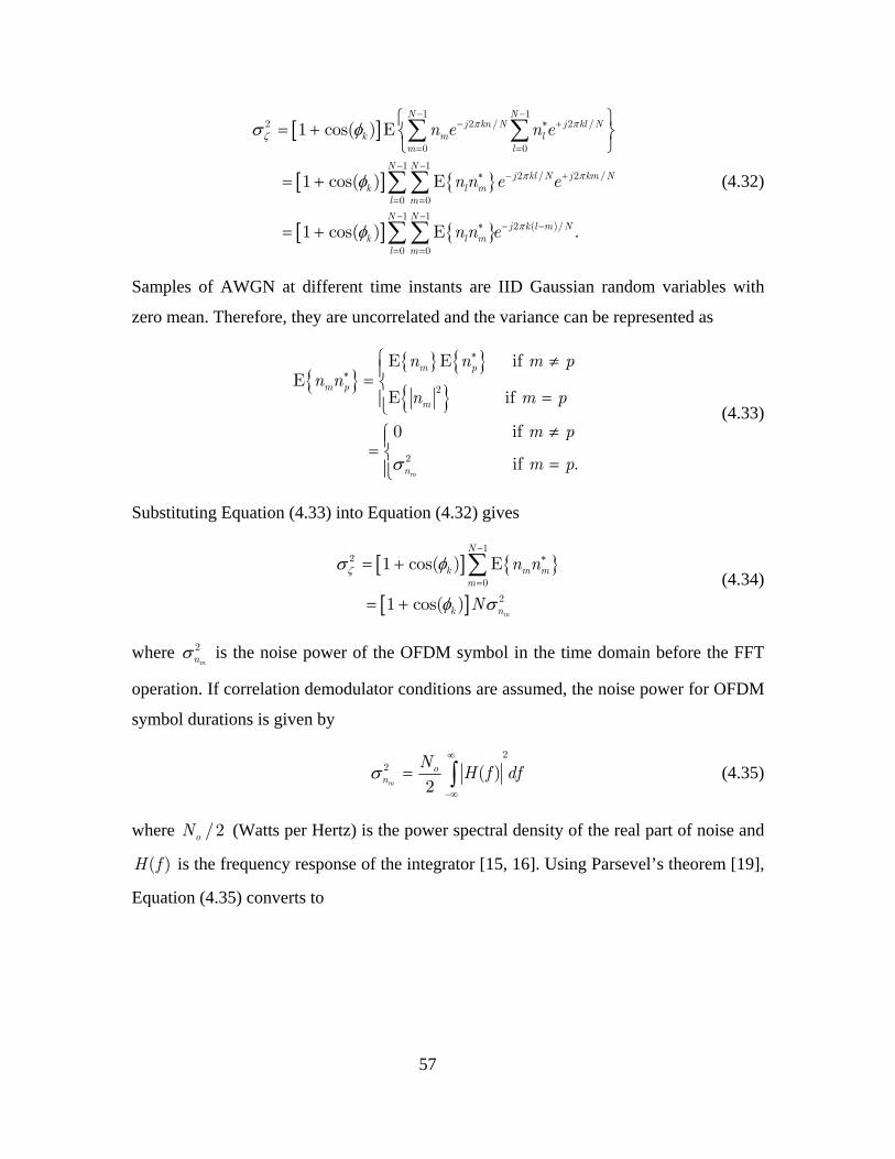
57

[ ]

[ ] { }

[ ] { }

π πζ

π π

π

σ φ

φ

φ

− −− ∗ +

= =

− −∗ − +

= =

− −∗ − −

= =

⎧ ⎫= + ⎨ ⎬

⎩ ⎭

= +

= +

∑ ∑

∑∑

∑∑

1 12 2 / 2 /

0 0

1 12 / 2 /

0 0

1 12 ( )/

0 0

1 cos( ) E

1 cos( ) E

1 cos( ) E .

N Nj kn N j kl N

k m lm l

N Nj kl N j km N

k l ml m

N Nj k l m N

k l ml m

n e n e

n n e e

n n e

(4.32)

Samples of AWGN at different time instants are IID Gaussian random variables with

zero mean. Therefore, they are uncorrelated and the variance can be represented as

{ }{ } { }{ }

σ

∗

∗⎧ ≠⎪= ⎨

=⎪⎩≠⎧⎪= ⎨ =⎪⎩

2

2

E E if E

E if

0 if

if .m

m p

m p

m

n

n n m pn n

n m p

m p

m p

(4.33)


[ ] { }

[ ]

ζσ φ

φ σ

−∗

=

= +

= +

∑1

2

0

2

1 cos( ) E

1 cos( )m

N

k m mm

k n

n n

N (4.34)

where 2

mnσ is the noise power of the OFDM symbol in the time domain before the FFT

operation. If correlation demodulator conditions are assumed, the noise power for OFDM

symbol durations is given by

2

2 ( )2m

on

NH f dfσ

∞

−∞

= ∫ (4.35)

where /2oN (Watts per Hertz) is the power spectral density of the real part of noise and

( )H f is the frequency response of the integrator [15, 16]. Using Parsevel’s theorem [19],

Equation (4.35) converts to

58

σ =

=

=

∫

∫

22

0

20

[ ]2

1

2

.2

s

m

s

To

n

To

s

o

s

Nh t dt

Ndt

T

NT

(4.36)


[ ]ζ

φσ

+=2 1 cos( )

.2k o

s

NN

T (4.37)

Substituting, sT from Equation (2.33) and since for BPSK 's bT T= , Equation (4.37)

yields

[ ] [ ]ζ

φ φσ

+ += =2 1 cos( ) 1 cos( )

.2 2

k o k o

b b

NN N

NT T (4.38)

Using Equations (4.24) and (4.38), the bit error probability 'bP conditioned on the value

kφ can be expressed as

{ }

[ ]

[ ] [ ]

ξ ξ

ξ ξ

ξ

ζ

ζ ζ ζσ σ

ζ ζ ζσ σ

ζ φσ φ

φ φ

+ +

+ +

+

= <

⎧ ⎫−⎪ ⎪= < −⎨ ⎬⎪ ⎪⎩ ⎭⎧ ⎫−⎪ ⎪= >⎨ ⎬⎪ ⎪⎩ ⎭

⎛ ⎞⎛ ⎞ +⎜ ⎟= =⎜ ⎟⎜ ⎟ ⎜ ⎟+⎝ ⎠ ⎝ ⎠⎛ ⎞ ⎛+ +⎜ ⎟ ⎜= =⎜ ⎟ ⎝⎝ ⎠

' Pr 0 | " 0 " was sent

Pr | " 0 "

Pr | " 0 "

2 (1 cos( ))

1 cos( ) /2

2 1 cos( ) 1 cos( ) 2

k k

k k

k

b k

k k k

k k k

k k

k o b

b k b k

o o

P

AQ Q

N T

A T EQ Q

N N

⎞⎟

⎜ ⎟⎠.

(4.39)

The number of data symbols per OFDM frame is 192 as discussed in Chapter III.

The indices of these data symbols are given as 9,10,...,100,156,157,...,255k = . Thus,

the average bit error probability bP is given by

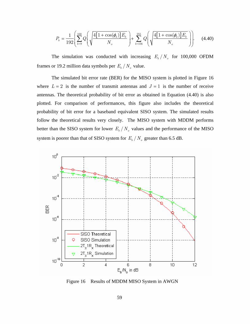
59

[ ] [ ]φ φ

= =

⎛ ⎞⎛ ⎞ ⎛ ⎞+ +⎜ ⎟⎜ ⎟ ⎜ ⎟= +

⎜ ⎟ ⎜ ⎟⎜ ⎟⎝ ⎠ ⎝ ⎠⎝ ⎠∑ ∑100 255

9 156

4 1 cos( ) 4 1 cos( )1.

192k b k b

bk ko o

E EP Q Q

N N (4.40)

The simulation was conducted with increasing /b oE N for 100,000 OFDM

frames or 19.2 million data symbols per /b oE N value.

The simulated bit error rate (BER) for the MISO system is plotted in Figure 16

where 2L = is the number of transmit antennas and 1J = is the number of receive

antennas. The theoretical probability of bit error as obtained in Equation (4.40) is also

plotted. For comparison of performances, this figure also includes the theoretical

probability of bit error for a baseband equivalent SISO system. The simulated results

follow the theoretical results very closely. The MISO system with MDDM performs

better than the SISO system for lower /b oE N values and the performance of the MISO

system is poorer than that of SISO system for /b oE N greater than 6.5 dB.

Figure 16 Results of MDDM MISO System in AWGN

60

2. Performance Analysis of MIMO System with Two Transmit and Two Receive Antennas

For the MDDM MIMO system with two receive antennas, it is assumed that the

signal receptions at both the antennas are uncorrelated and signals are received at the

same time without any relative delay. The received signals at both receive antennas are

given by

1 1 2 1

2 1 2 2 .

m m m m

m m m m

r x x n

r x x n

= + +

= + + (4.41)

After the FFT operation the signals can be represented as

1 1 2 1

2 1 2 2.

k k k k

k k k k

R X X N

R X X N

= + +

= + + (4.42)

Substituting Equation (2.31) and (4.19) into Equation (4.42) gives

1 1 1 2 / 1

2 1 1 2 / 2

1 1 1

2 1 2

(1 )

(1 ) .

k

k

j k Nk k k k

j k Nk k k k

jk k k

jk k k

R X X e N

R X X e N

R e X N

R e X N

π

π

φ

φ

−

−

−

−

= + +

= + +

= + +

= + +

(4.43)

Following the derivation of Equation (4.23), Equation (4.43) converts to

[ ][ ]

φ φ

φ φ

φ

φ

+ +

+ +

= + = + + +

= + = + + +

1 1 1 1

2 2 1 2

(1 ) 2 2 cos( ) (1 )

(1 ) 2 2 cos( ) (1 ) .

k k

k k

j jk k k k k

j jk k k k k

Z R e X e N

Z R e X e N (4.44)

Now both space diversity receptions are combined to form random variable kZ which is

given by

[ ]

[ ]

[ ]

φ φ

φ φ

φ φ

φ

φ

φ

+ +

+ +

+ +

= +

= + + + + +

= + + + + +

= + + + + +

1 2

1 1 2

1 2

1 2

4 4 cos( ) (1 ) (1 )

4 1 cos( ) (1 ) (1 )2

2 2 1 cos( ) (1 ) (1 ) .

k k

k k

k k

k k k

j jk k k k

j jk k k

j jk k k

Z Z Z

X e N e N

Ae N e N

A e N e N

(4.45)

If correlation demodulator conditions are assumed, then

61

{ }0

1E | " 0" was transmitted E

2 2 (1 cos( )).

bT

k kb

k

Z Z dtT

A φ

⎧ ⎫⎪ ⎪= ⎨ ⎬⎪ ⎪⎩ ⎭

= +

∫ (4.46)

The variance of { }ζ = Rek kZ is only due to the variance of real part of noise

components [15, 16]. Noise components at both receive antennas are IID Gaussian

random variables. Therefore the total variance of the sum of two noise components is the

sum of their individual variances [18]. The total noise variance is given as

ζ ζ ζσ σ σ= +1 22 2 2

k k k (4.47)

where { }ζ =1 1Rek kZ and { }ζ =2 2Re .k kZ Following the derivation of noise variance

derived in Equation (4.37), Equation (4.47) is represented as

[ ] [ ]

[ ]

ζ

φ φσ

φ

+ += +

+=

2 1 cos( ) 1 cos( )

2 2

1 cos( )

k

k o k o

b b

k o

b

N N

T T

N

T

(4.48)

and ζσ k is given as

ζφσ +

=(1 cos( ))

.k

k o

b

NT

(4.49)

Following the derivation of Equation (4.39), the bit error probability 'bP conditioned on

the value kφ is given by

[ ][ ]

[ ]

[ ]

φ

φ

φ

φ

⎛ ⎞+⎜ ⎟=⎜ ⎟+⎝ ⎠⎛ ⎞+⎜ ⎟=⎜ ⎟⎝ ⎠⎛ ⎞+⎜ ⎟=⎜ ⎟⎝ ⎠

'

2

2 2 1 cos( )

1 cos( ) /

8 1 cos( )

8 1 cos( ) .

kb

k o b

k b

o

k b

o

AP Q

N T

ATQ

N

EQ

N

(4.50)

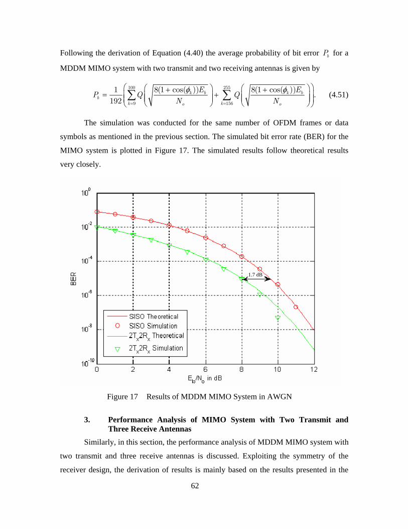
62

Following the derivation of Equation (4.40) the average probability of bit error bP for a

MDDM MIMO system with two transmit and two receiving antennas is given by

100 255

9 156

1 8(1 cos( )) 8(1 cos( )).

192k b k b

bk ko o

E EP Q Q

N Nφ φ

= =

⎛ ⎞⎛ ⎞ ⎛ ⎞+ += +⎜ ⎟⎜ ⎟ ⎜ ⎟⎜ ⎟ ⎜ ⎟⎜ ⎟⎝ ⎠ ⎝ ⎠⎝ ⎠

∑ ∑ (4.51)

The simulation was conducted for the same number of OFDM frames or data

symbols as mentioned in the previous section. The simulated bit error rate (BER) for the

MIMO system is plotted in Figure 17. The simulated results follow theoretical results

very closely.

Figure 17 Results of MDDM MIMO System in AWGN

3. Performance Analysis of MIMO System with Two Transmit and

Three Receive Antennas Similarly, in this section, the performance analysis of MDDM MIMO system with

two transmit and three receive antennas is discussed. Exploiting the symmetry of the

receiver design, the derivation of results is mainly based on the results presented in the

1.7 dB

63

last two sections. It is also assumed that the signal receptions at all antennas are

uncorrelated and signals are received at the same time without any relative delay. The

received signals at the three receive antennas are given by

1 1 2 1

2 1 2 2

3 1 2 3 .

m m m m

m m m m

m m m m

r x x n

r x x n

r x x n

= + +

= + +

= + +

(4.52)

After the FFT operation the signals are represented as

1 1 2 1

2 1 2 2

3 1 2 3.

k k k k

k k k k

k k k k

R X X N

R X X N

R X X N

= + +

= + +

= + +

(4.53)

Based on the discussion in previous sections, the components of the variables from all the

space diversity receptions are

[ ][ ][ ]

φ φ

φ φ

φ φ

φ

φ

φ

+ +

+ +

+ +

= + = + + +

= + = + + +

= + = + + +

1 1 1 1

2 2 1 2

3 3 1 3

(1 ) 2 2 cos( ) (1 )

(1 ) 2 2 cos( ) (1 )

(1 ) 2 2 cos( ) (1 ) .

k k

k k

k k

j jk k k k k

j jk k k k k

j jk k k k k

Z R e X e N

Z R e X e N

Z R e X e N

(4.54)

Now all the space diversity receptions are combined to form random variable kZ which

is given by

[ ] φ φ φφ

= + +

= + + + + + + +

1 2 3

1 1 2 3 6 1 cos( ) (1 ) (1 ) (1 ) .k k k

k k k k

j j jk k k k k

Z Z Z Z

X e N e N e N (4.55)

If correlation demodulator conditions are assumed, then

{ } ( ) ( )

[ ]

φφ

φ

+⎧ ⎫⎪ ⎪⎡ ⎤= + + +⎨ ⎬⎣ ⎦⎪ ⎪⎩ ⎭= +

∫0

1E | " 0" was transmitted E 2 2 1 cos 1

2 2 1 cos( ) .

b

k

Tj

k k kb

k

Z A N e dtT

A

(4.56)

The variance of { }ζ = Rek kZ is only due to the variance of real part of noise

components [15, 16]. Noise components at all the receive antennas are IID Gaussian

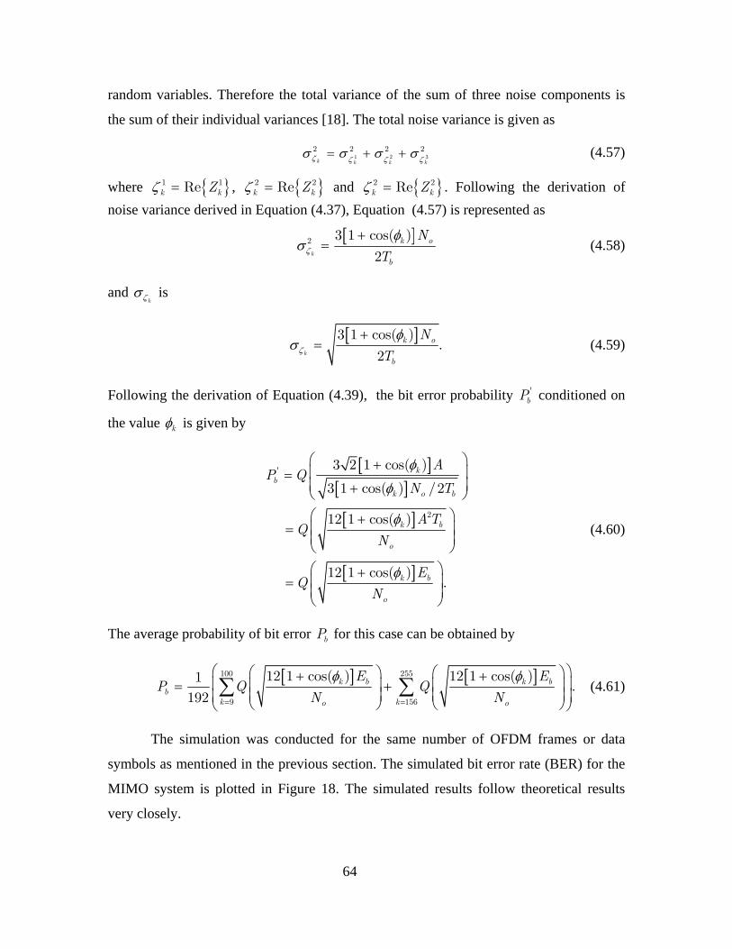
64

random variables. Therefore the total variance of the sum of three noise components is

the sum of their individual variances [18]. The total noise variance is given as

ζ ζ ζ ζσ σ σ σ= + +1 2 32 2 2 2

k k k k (4.57)

where { }ζ =1 1Rek kZ , { }ζ =2 2Rek kZ and { }ζ =2 2Rek kZ . Following the derivation of noise variance derived in Equation (4.37), Equation (4.57) is represented as

[ ]ζ

φσ

+=2 3 1 cos( )

2k

k o

b

N

T (4.58)

and ζσ k is

[ ]ζ

φσ

+=

3 1 cos( ).

2k

k o

b

N

T (4.59)

Following the derivation of Equation (4.39), the bit error probability 'bP conditioned on

the value kφ is given by

[ ][ ]

[ ]

[ ]

φ

φ

φ

φ

⎛ ⎞+⎜ ⎟=⎜ ⎟+⎝ ⎠⎛ ⎞+⎜ ⎟=⎜ ⎟⎝ ⎠⎛ ⎞+⎜ ⎟=⎜ ⎟⎝ ⎠

'

2

3 2 1 cos( )

3 1 cos( ) /2

12 1 cos( )

12 1 cos( ) .

kb

k o b

k b

o

k b

o

AP Q

N T

ATQ

N

EQ

N

(4.60)

The average probability of bit error bP for this case can be obtained by

[ ] [ ]φ φ

= =

⎛ ⎞⎛ ⎞ ⎛ ⎞+ +⎜ ⎟⎜ ⎟ ⎜ ⎟= +

⎜ ⎟ ⎜ ⎟⎜ ⎟⎝ ⎠ ⎝ ⎠⎝ ⎠∑ ∑100 255

9 156

12 1 cos( ) 12 1 cos( )1.

192k b k b

bk ko o

E EP Q Q

N N (4.61)

The simulation was conducted for the same number of OFDM frames or data

symbols as mentioned in the previous section. The simulated bit error rate (BER) for the

MIMO system is plotted in Figure 18. The simulated results follow theoretical results

very closely.

65

A comparison of Equations (4.40), (4.51) and (4.61) clearly reveals that the

improvement factor increases linearly with increasing number of receiving antenna. Thus,

the average probability of bit error in AWGN channel for MDDM scheme discussed in

this thesis with J receiving antenna can be represented in general form as

100 255

9 156

1 4 (1 cos( )) 4 (1 cos( )).

192k b k b

bk ko o

J E J EP Q Q

N Nφ φ

= =

⎛ ⎞⎛ ⎞ ⎛ ⎞+ += +⎜ ⎟⎜ ⎟ ⎜ ⎟⎜ ⎟ ⎜ ⎟⎜ ⎟⎝ ⎠ ⎝ ⎠⎝ ⎠

∑ ∑ (4.62)

Figure 18 Results of MDDM MIMO System in AWGN

D. SIMULATION AND PERFORMANCE ANALYSIS OF MDDM IN A

MULTIPATH FADING CHANNEL Next, the MDDM scheme was simulated and analyzed with the effect of a slow

fading frequency nonselective channel. The multipath model for the slow Rayleigh fading

channel was discussed in Chapter II. A multipath fading channel is inserted in Figure 15

from each transmit antenna to each receive antenna. A block diagram of the MIMO

3.4 dB

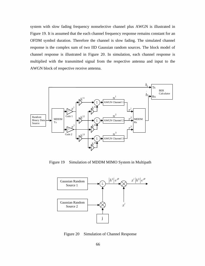
66

system with slow fading frequency nonselective channel plus AWGN is illustrated in

Figure 19. It is assumed that the each channel frequency response remains constant for an

OFDM symbol duration. Therefore the channel is slow fading. The simulated channel

response is the complex sum of two IID Gaussian random sources. The block model of

channel response is illustrated in Figure 20. In simulation, each channel response is

multiplied with the transmitted signal from the respective antenna and input to the

AWGN block of respective receive antenna.

MDDM Tx

Random Binary Data Source

AWGN Channel 1

g

∑

g

∑

∑

AWGN Channel 3

AWGN Channel 2 MDDM Rx

BER Calculator

Tx

Rx 1n

2n

3n

Gain 1

Gain 2

1r

2r

3r 2x

1x

kb

^

kb 11h

23h

22h

12h

13h

21h

Figure 19 Simulation of MDDM MIMO System in Multipath

Figure 20 Simulation of Channel Response

Gaussian Random Source 1

Gaussian Random Source 2

j

∑

lj jh e θ l lj jx h e θ

lx

67

Each Gaussian random source generates a zero mean random variable. In this

simulation model, the variance of each Gaussian source is equal and is set to a value such

that the variance of the complex sum of these Gaussian random sources is one. Using

Equation (2.52), the channel response from transmit antenna l to receive antenna j is

represented as

ljjlj ljh h e

X jY

θ=

= + (4.63)

where X and Y are IID Gaussian random variables with zero mean and equal variance.

The variance of the complex sum can be given as

{ } { }( )( ) ( ){ }{ }

22 *

*

2 2

2 2

1.

ljlj lj lj

h

X Y

E h h E h

E X jY X jY

E X Y

σ

σ σ

= −

= + +

= +

= +

=

(4.64)

Thus the variance of each Gaussian random source was set as

2 2 1/2.X Yσ σ= = (4.65)

1. Performance Analysis of MISO System with Two Transmit and One Receive Antenna

At the receive antenna, the signal mr is written as

11 1 21 2m m m mr h x h x n= + + . (4.66)

where 11h and 21h are channel responses from transmit antenna 1 and 2 to the receive

antenna respectively. These channel responses are assumed independent. After the FFT

operation, the signal is written as

= + +11 1 21 2FFT[ ] FFT[ ].m m m mr h x h x n (4.67)

All the channel responses are considered constant for the duration of an OFDM symbol

for the slow fading channel. Now, Equation (4.67) can be written as

11 1 21 2k k k kR h X h X N= + + . (4.68)

68

Substituting Equation (2.31) , (4.16) and (4.20) into Equation (4.68) yields

11 1 21 1

11 21 1( )

k

k

jk k k k

jk k k

R h X h X e N

R h h e X N

φ

φ

−

−

= + +

= + + (4.69)

where kN is AWGN in the frequency domain and 11 21( )kjh h e φ−+ is the effective channel

response for the MDDM in the multipath channel. In Equation (4.69) 21h is a random

variable with Rayleigh distributed amplitude and phase uniformly distributed on ( ]π π− , .

Thus, multiplying 21h by kje φ− does not change the statistics of the random variable and

their product is represented as 21'h . Now, the effective channel response can be written as

1 11 21'H h h= + (4.70)

Using the MRC receiver as shown in Figure 14, Equation (4.69) is multiplied by

the complex conjugate of the effective channel response and the and random variable kZ

is represented as

1 1* 1 1*k k kZ H H X H N= + . (4.71)

Now, Equation (4.71) can be written as

( ) ( ) ( )( ) ( )

21 1 1*

* *11 21' 11 21' 1 11 21'

2 *211 21' 11 21' 11 21' 1 11 21'

2( )

k k k

k k

I I Q Q k k

Z H X H N

h h h h X h h N

h h h h h h X h h N

= +

= + + + +

= + + + + +

(4.72)

where lj lj ljI Qh h jh= + , i.e. lj

Ih and ljQh are the inphase and quadrature components of the

respective channel responses.

For a fixed set of channel responses Equation (4.72) represents a complex

Gaussian random variable kZ due to AWGN [16]. To demodulate the BPSK signal, the

real part of the decision variable kZ , { }ζ = Rek kZ , is compared with a threshold as

given in Table 3. If correlation demodulator conditions are assumed, then

69

{ }{ }

( ) ( )

( )

ζ + =

⎧ ⎫⎪ ⎪⎡ ⎤= + + + + +⎨ ⎬⎣ ⎦⎪ ⎪⎩ ⎭

⎡ ⎤= + + +⎣ ⎦

∫2 *211 21' 11 21' 11 21' 1 11 21'

0

2211 21' 11 21' 11 21'

E Re | " 0 " was transmitted

1 E 2

22

b

k k

T

I I Q Q k kb

I I Q Q

Z

h h h h h h X h h N dtT

Ah h h h h h

(4.73)

The variance of ζ k is only due to the variance of real part of the noise component 1*

kH N [15, 16] and is represented as

( ){ } { }( )( ){ }

ζσ ⎡ ⎤ ⎡ ⎤= −⎣ ⎦ ⎣ ⎦

⎡ ⎤= ⎣ ⎦

222 1* 1*

21*

E Re E Re

E Re

k k k

k

H N H N

H N (4.74)

where { }E represents the expected value. ηk is the real part of noise component with

zero mean which can be written as

( )1* 1* 1 *1Re

2k k k kH N H N H Nη ⎡ ⎤= = +⎣ ⎦ (4.75)

And

( ) ( )

( ) ( ) ( )( )( ) ( ) ( )( )

222 1* 1* 1 *

2 2 21* 2 1 1 1*

2 22 21* 2 1 1

1Re

21

241

2 .4

k k k k

k k k k

k k k k

H N H N H N

H N H N H H N N

H N H N H N N

η

∗ ∗

∗ ∗

⎛ ⎞⎡ ⎤= = +⎜ ⎟⎣ ⎦ ⎝ ⎠

= + +

= + +

(4.76)


( ) ( ) ( )( ){ }

( ) ( ){ } ( ) ( ){ } { }( )ζσ

∗ ∗

∗ ∗

= + +

= + +

2 22 22 1* 2 1 1

2 22 221* 1 1

1E 2

41

E E 2 E .4

k k k k k

k k k k

H N H N H N N

H N H N H N N (4.77)

kN is a complex Gaussian random variable with zero mean, therefore

( ){ } ( ){ }220k kE N E N ∗= = . (4.78)


70

{ }

( ) { }

ζσ∗

∗

=

= + + +

22 1

2211 21' 11 21' 11 21'

2E

41

2( ) E .2

k k k

I I Q Q k k

H N N

h h h h h h N N (4.79)


( )

( )

ζ

ζ

σ

σ

⎡ ⎤= + + +⎣ ⎦

⎡ ⎤= + + +⎣ ⎦

222 11 21' 11 21' 11 21'

2211 21' 11 21' 11 21'

12

2 2

2 .4

k

k

oI I Q Q

b

oI I Q Q

b

Nh h h h h h

T

Nh h h h h h

T

(4.80)

Now, the conditional bit error probability can be represented as

{ }

( )( )

ζ ζ

ζ ζ

ζ

ζ

ζ ζ ζσ σ

ζ ζ ζσ σ

ζσ

+ +

+ +

+

= <

⎧ ⎫−⎪ ⎪= < −⎨ ⎬⎪ ⎪⎩ ⎭⎧ ⎫−⎪ ⎪= >⎨ ⎬⎪ ⎪⎩ ⎭⎛ ⎞

= ⎜ ⎟⎜ ⎟⎝ ⎠⎛

+ + +⎜= ⎜

⎜ + + +⎝

'

2211 21' 11 21' 11 21'

2211 21' 11 21' 11 21'

Pr 0 | " 0 " was sent

Pr | " 0 "

Pr | " 0 "

2( ) / 2

2( ) /4

k k

k k

k

b k

k k k

k k k

k

I I Q Q

I I Q Q o b

P

Q

h h h h h h AQ

h h h h h h N T

( )

⎞⎟⎟⎟⎠

⎛ ⎞+ + +⎜ ⎟= ⎜ ⎟

⎜ ⎟⎝ ⎠

222 11 21' 11 21' 11 21'2 2( )

b I I Q Q

o

AT h h h h h hQ

N (4.81)

or

' 11

2( ) bb

o

EP Q

Nββ

⎛ ⎞= ⎜ ⎟⎜ ⎟

⎝ ⎠ (4.82)

where 1β is given as

( )β = + + +2211 21' 11 21' 11 21'

1 2 .I I Q Qh h h h h h (4.83)

Equation (4.82) depicts the bit error probability of a MDDM MISO system conditioned

on the random variable 1β . The performance of an MDDM MISO system over a

71

frequency nonselective, slowly fading Rayleigh channel with MRC can be obtained by

taking the average of the conditional bit error probability over all possible values of the

random variable 1β . Now, the unconditional bit error probability can be given as

( )

( ) ( )

β β β

β β β

∞

Β

∞

Β

=

=

∫

∫

1

1

1 1 10

1 1 10

( )

2 /

b b

b o

P P f d

Q E N f d (4.84)

where ( )1 1f βΒ is the probability density function for 1β .

The random variable 1β as defined in Equation (4.83) is a sum of two central chi

squared random variables of degree two, 211h and

221'h , and two products of Gaussian

random variables, 11 21'2 I Ih h and 11 21'2 Q Qh h . These central chi squared random variables and

Gaussian random variables are also correlated. The probability density function of the

random variable 1β and integral of Equation (4.84) were computed numerically.

The random variable 1β was generated in Matlab by taking one million samples

each of channel response 11h and 21'h . The effective channel response was multiplied by

its complex conjugate. The distribution of 1β over its range was obtained by evaluating a

histogram of 500 equally spaced bins with the help of the Matlab function hist . The

distribution of the data was interpolated by cubic spline data interpolation with the help

of the Matlab function spline . After data interpolation, this data distribution curve was

normalized to make the total area under the distribution curve equal to one. Then, the

probability over all possible values was interpolated by using the Matlab function spline .

At the end, the average probability of bit error was computed numerically over all the

possible values of the random variable 1β . The Matlab code is presented in Appendix B.

[21]

The simulated and the numerically computed theoretical results of a MISO system

over frequency nonselective slowly fading Rayleigh channel are shown in Figure 21. For

the comparison of the performances, the theoretical bit error rate (BER) of the BPSK

SISO system as obtained in Equation (2.127) is also plotted along with the bit error

probability obtained from the simulation. The simulated results are close to the

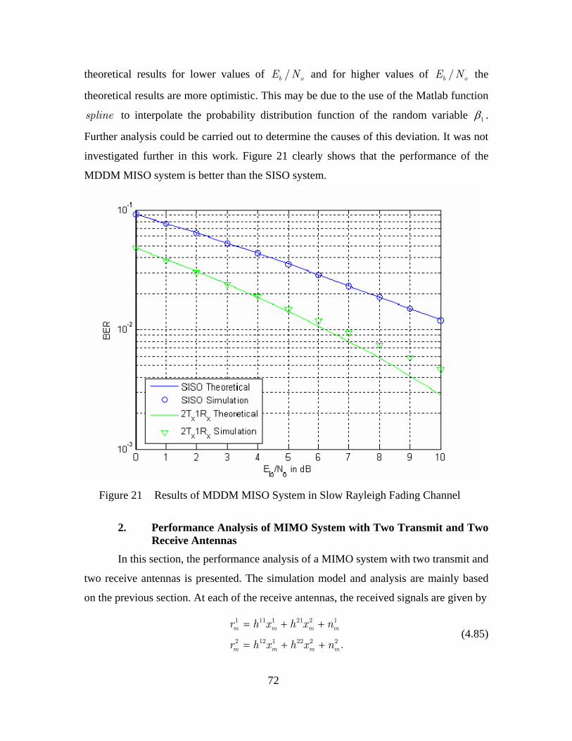
72

theoretical results for lower values of /b oE N and for higher values of /b oE N the

theoretical results are more optimistic. This may be due to the use of the Matlab function

spline to interpolate the probability distribution function of the random variable 1β .

Further analysis could be carried out to determine the causes of this deviation. It was not

investigated further in this work. Figure 21 clearly shows that the performance of the

MDDM MISO system is better than the SISO system.

Figure 21 Results of MDDM MISO System in Slow Rayleigh Fading Channel

2. Performance Analysis of MIMO System with Two Transmit and Two

Receive Antennas In this section, the performance analysis of a MIMO system with two transmit and

two receive antennas is presented. The simulation model and analysis are mainly based

on the previous section. At each of the receive antennas, the received signals are given by

1 11 1 21 2 1

2 12 1 22 2 2 .

m m m m

m m m m

r h x h x n

r h x h x n

= + +

= + + (4.85)

73

where ljh represents channel response from transmit antenna l to receive antenna j and jmr is the received signal at receive antenna j . It is considered that all the channel

responses are independent and the reception of the signals at both the antennas is

uncorrelated. After the FFT operation the signals are represented as

⎡ ⎤ = ⎡ + + ⎤⎣ ⎦ ⎣ ⎦

⎡ ⎤ = ⎡ + + ⎤⎣ ⎦ ⎣ ⎦

1 11 1 21 2 1

2 12 1 22 2 2

FFT FFT

FFT FFT .

m m m m

m m m m

r h x h x n

r h x h x n (4.86)

All the channel responses are considered constant for the duration of an OFDM symbol.


1 11 1 21 2 1

2 12 1 22 2 2.

k k k k

k k k k

R h X h X N

R h X h X N

= + +

= + + (4.87)

Substituting Equations (2.31) , (4.16) and (4.20) into Equations (4.87) yields

1 11 1 21 1 1

2 12 1 22 1 2

1 11 21 1 1

2 12 22 1 2

( )

( )

k

k

k

k

jk k k k

jk k k k

jk k k

jk k k

R h X h X e N

R h X h X e N

R h h e X N

R h h e X N

φ

φ

φ

φ

−

−

−

−

= + +

= + +

= + +

= + +

(4.88)

where jkN is AWGN in the frequency domain at receive antenna j , ( )φ−+11 21 kjh h e is the

effective channel response at receive antenna 1 and ( )φ−+12 22 kjh h e is the effective

channel response at receive antenna 2 . In Equation (4.88), all ( ) 1, 2 and 1, 2ljh l j= =

are random variables with Rayleigh distributed amplitude and phase uniformly

distributed on ( ]π π− , . Thus, multiplying 21h and 22h by kje φ− does not change the

statistics of both the random variables and their respective products are represented as 21' 21 kjh h e φ−= and φ−=22' 22 kjh h e . Now, the effective channel responses are written as

1 11 21'

2 12 22'.

H h h

H h h

= +

= + (4.89)

74

Using the MRC receiver as shown in Figure 14, Equation (4.88) is multiplied by

the complex conjugate of the effective channel response and the random variables for

respective diversity receptions are given by

1 1 1* 1 1* 1

2 2 2* 1 2* 2

21 1 1 1* 1

22 2 1 2* 2.

k k k

k k k

k k k

k k k

Z H H X H N

Z H H X H N

Z H X H N

Z H X H N

= +

= +

= +

= +

(4.90)

Now Equations (4.90) can be expressed as

( ) ( )

( ) ( )

2 *21 11 21' 11 21' 11 21' 1 11 21' 1

2 *22 12 22' 12 22' 12 22' 1 12 22' 2

2( )

2( )

k I I Q Q k k

k I I Q Q k k

Z h h h h h h X h h N


= + + + + +

= + + + + + (4.91)

where { }Relj ljIh h= and { }Imlj lj

Qh h= are the inphase and quadrature components of the respective channel responses.

After combining both the space diversity receptions in the MRC receiver the

decision variable kZ is given as

( )

1 2

2 21 1 2 1 1* 1 2* 2

2 21 2 1 1* 1 2* 2

.

k k k

k k k k

k k k

Z Z Z

H X H X H N H N

H H X H N H N

= +

= + + +

= + + +

(4.92)



real part of the decision variable kZ , { }Rek kZζ = , is compared with a threshold as given

in Table 3. If correlation demodulator conditions are assumed, then

75

{ }{ }

( )( ) ( )

ζ

β

+ =

⎧ ⎫⎪ ⎪⎡ ⎤= + + +⎨ ⎬⎢ ⎥⎣ ⎦⎪ ⎪⎩ ⎭

⎡ ⎤= + + + + + + +⎣ ⎦

=

∫2 21 2 1 1* 1 2* 2

0

2 22 211 21' 11 21' 11 21' 12 22' 12 22' 12 22'

2


1 E

2 22

2

b

k k

T

k k kb

I I Q Q I I Q Q

Z

H H X H N H N dtT

Ah h h h h h h h h h h h

A

(4.93)

where

( )

( )

2 22 211 21' 12 22' 11 21' 11 21'2

12 22' 12 22'

2

2 .

I I Q Q

I I Q Q

h h h h h h h h

h h h h

β = + + + + + +

+ (4.94)

The variance of ζ k is only due to the variance of real part of the noise components 1* 1

kH N and 2* 2kH N [15, 16]. Noise components at both the receive antennas 1

kN and 2kN

are IID complex Gaussian random variables. Thus, the variance of their sum is the sum of their individual variances and is given as

ζ ζ ζσ σ σ= +1 22 2 2 .k k k

(4.95)

Following the results derived in the previous section from Equation (4.74) to (4.80), ζσ2

k

can be expressed as

{ } { }

( )( )

ζσ∗ ∗= +

⎡ ⎤+ + + +⎢ ⎥=⎢ ⎥+ + +⎣ ⎦

2 22 1 1 1 2 2 2

2211 21' 11 21' 11 21'

02212 22' 12 22' 12 22'

1 1E E

2 2

2 .

4 2

k k k k k

I I Q Q

b I I Q Q

H N N H N N

h h h h h hNT h h h h h h

(4.96)

Substituting Equation (4.94) into Equation (4.96) yeilds

ζ

ζ

βσ

βσ

=

=

2 0 2

0 2

4

.4

k

k

b

b

NT

NT

(4.97)

Now, substituting Equation (4.93) and (4.97) into Equation (4.3), the conditional bit error

probability is represented as

76

22

2

2

/ 2( )

/4

2 .

b

o b

b

o

AP Q

N T

EQ

N

βββ

β

⎛ ⎞= ⎜ ⎟⎜ ⎟

⎝ ⎠⎛ ⎞

= ⎜ ⎟⎜ ⎟⎝ ⎠

(4.98)

Equation (4.98) represents the bit error probability of an MDDM MIMO system

with two transmit antennas and two receive antennas conditioned on a random variable

2β . The performance of the MDDM MIMO system over a frequency nonselective slowly

fading Rayleigh channel with MRC can be obtained by taking the average of the

conditional bit error probability over all possible values of random variable 2β . Now the

unconditional bit error probability can be given as

( )

( ) ( )

β β β

β β β

∞

Β

∞

Β

=

=

∫

∫

2

2

2 2 20

2 2 20

( )

2 /

b b

b o

P P f d

Q E N f d (4.99)


The random variable 2β as defined in Equation (4.94) is a sum of central chi

squared random variables of degree two and products of Gaussian random variables. The

central chi squared random variables and Gaussian random variables are also correlated.

The probability density function of the random variable 2β and integral of Equation

(4.99) were computed numerically, using the same algorithm as discussed in previous

section.

The simulated and the numerically computed theoretical results of the MIMO

system with two transmit antennas and two receive antennas over a frequency

nonselective slowly fading Rayleigh channel are shown in Figure 22. For the comparison

of the performances, this figure also includes the theoretical and the simulated bit error

probability of a BPSK SISO system. The simulation results, for low /b oE N values,

deviate slightly from the theoretical results. The theoretical results are more optimistic for

low /b oE N . The reason for this slight deviation may be the same as discussed in the

previous section, however, this was not investigated in this work.

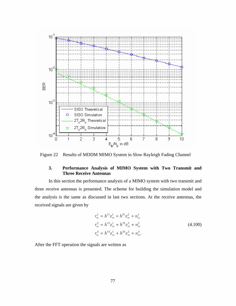
77

Figure 22 Results of MDDM MIMO System in Slow Rayleigh Fading Channel

3. Performance Analysis of MIMO System with Two Transmit and

Three Receive Antennas In this section the performance analysis of a MIMO system with two transmit and

three receive antennas is presented. The scheme for building the simulation model and

the analysis is the same as discussed in last two sections. At the receive antennas, the

received signals are given by

1 11 1 21 2 1

2 12 1 22 2 2

3 13 1 23 2 3 .

m m m m

m m m m

m m m m

r h x h x n

r h x h x n

r h x h x n

= + +

= + +

= + +

(4.100)

After the FFT operation the signals are written as

78

⎡ ⎤ = ⎡ + + ⎤⎣ ⎦ ⎣ ⎦

⎡ ⎤ = ⎡ + + ⎤⎣ ⎦ ⎣ ⎦

⎡ ⎤ = ⎡ + + ⎤⎣ ⎦ ⎣ ⎦

1 11 1 21 2 1

2 12 1 22 2 2

3 13 1 23 2 3

FFT FFT

FFT FFT

FFT FFT .

m m m m

m m m m

m m m m

r h x h x n

r h x h x n

r h x h x n

(4.101)

All the channel responses are considered fixed for the duration of an OFDM symbol.


1 11 1 21 2 1

2 12 1 22 2 2

3 13 1 23 2 3.

k k k k

k k k k

k k k k

R h X h X N

R h X h X N

R h X h X N

= + +

= + +

= + +

(4.102)

Substituting Equations (2.31), (4.16) and (4.20) into Equations (4.102) yields

1 11 1 21 1 1

2 12 1 22 1 2

3 13 1 23 1 3

1 11 21 1 1

2 21 22 1 2

3 13 23 1 3

( )

( )

( )

k

k

k

k

k

k

jk k k k

jk k k k

jk k k k

jk k k

jk k k

jk k k

R h X h X e N

R h X h X e N

R h X h X e N

R h h e X N

R h h e X N

R h h e X N

φ

φ

φ

φ

φ

φ

−

−

−

−

−

−

= + +

= + +

= + +

= + +

= + +

= + +

(4.103)

where kN is AWGN in the frequency domain. 11 21( )kjh h e φ−+ , 21 22( )kjh h e φ−+ and 13 23( )kjh h e φ−+ are the effective channel responses at receive antennas 1 , 2 and 3

respectively. In Equation (4.103), all ( ) 1, 2 and 1, 2, 3ljh l j= = are random variables

with Rayleigh distributed amplitude and phase uniformly distributed in ( ]π π− , . Thus,

multiplying 21h , 22h and 23h by kje φ− does not change the statistics of these random

variables and their respective products are represented as 21' 21 kjh h e φ−= , 22' 22 kjh h e φ−=

and 23' 23 kjh h e φ−= . Now, the effective channel responses are given as

1 11 21'

2 12 22'

3 13 23'.

H h h

H h h

H h h

= +

= +

= +

(4.104)

79

Using MRC receiver as shown in Figure 14, Equation (4.88) is multiplied by the

complex conjugate of the effective channel response and the random variable jkZ at

respective diversity receptions are written as

= +

= +

= +

= +

= +

= +

1 1 1* 1 1* 1

2 2 2* 1 2* 2

3 3 3* 1 3* 3

21 1 1 1* 1

22 2 1 2* 2

23 3 1 3* 3.

k k k

k k k

k k k

k k k

k k k

k k k

Z H H X H N

Z H H X H N

Z H H X H N

Z H X H N

Z H X H N

Z H X H N

(4.105)

Now, Equations (4.105) can be represented as

( ) ( )

( ) ( )

( ) ( )

⎡ ⎤= + + + + +⎣ ⎦⎡ ⎤= + + + + +⎣ ⎦⎡ ⎤= + + + + +⎣ ⎦

2 *21 11 21' 11 21' 11 21' 1 11 21' 1

2 *22 12 22' 12 22' 12 22' 1 12 22' 2

2 *23 13 23' 13 23' 13 23' 1 13 23' 3

2

2

2

k I I Q Q k k

k I I Q Q k k

k I I Q Q k k




(4.106)

where { }Relj ljIh h= and { }Imlj lj

Qh h= are the inphase and quadrature components of the respective channel responses.

After combining all the space diversity receptions in the MRC receiver the

decision variable kZ is given as

( )

1 2 3

2 2 21 1 2 1 3 1 1* 1 2* 2 3* 3

2 2 21 2 3 1 1* 1 2* 2 3* 3

.

k k k k

k k k k k k

k k k k

Z Z Z Z

H X H X H X H N H N H N

H H H X H N H N H N

= + +

= + + + + +

= + + + + +

(4.107)



real part of the decision variable kZ , { }ζ = Rek kZ , is compared with a threshold as

given in Table 3. If correlation demodulator conditions are assumed, then

80

{ }{ }

( )( )

( )( )

ζ + =

⎧ ⎫⎪ ⎪⎡ ⎤= + + + + +⎨ ⎬⎢ ⎥⎣ ⎦⎪ ⎪⎩ ⎭

= + +

+ + + + + +=

+ + +

∫2 2 21 2 3 1 1* 1 2* 2 3* 3

0

2 2 21 2 3 1

2 22 211 21' 11 21' 11 21' 12 22'

212 22' 12 22' 13 23


1 E

2

2 2

b

k k

T

k k k kb

k

I I Q Q

I I Q Q

Z

H H H X H N H N H N dtT

H H H X

h h h h h h h hA

h h h h h h ( )β

⎡ ⎤⎢ ⎥⎢ ⎥+ +⎣ ⎦

=

2' 13 23' 13 23'

3

2

2

I I Q Qh h h h

A

(4.108)

where

( )

( ) ( )β = + + + + + + + +

+ + +

2 2 22 2 211 21' 12 22' 13 23' 11 21' 11 21'3

12 22' 12 22' 13 23' 13 23'

2

2 2 .

I I Q Q

I I Q Q I I Q Q

h h h h h h h h h h

h h h h h h h h (4.109)

The variance of ζ k is only due to the variance of real part of the noise components 1* 1

kH N , 2* 2kH N and 3* 3

kH N [15, 16]. Noise components at all the receiving antennas 1kN , 2

kN and 3kN are IID complex Gaussian random variables. Thus, the variance of their

sum is the sum of their individual variances and is represented as

ζ ζ ζ ζσ σ σ σ= + +1 2 32 2 2 2 .k k k k

(4.110)

Following the results derived in previous section from Equation (4.74) to (4.80), 2kζ

σ can

be written as

{ } { } { }( )( )

( ) ( )

ζσ∗ ∗ ∗= + +

⎡ ⎤+ + + + + +⎢ ⎥=⎢ ⎥+ + + + +⎣ ⎦

2 2 22 1 1 1 2 2 2 3 3 3

2 22 211 21' 11 21' 11 21' 12 22'

02212 22' 12 22' 13 23' 13 23' 13 23'

1E E E

2

2 .

4 2 2

k k k k k k k

I I Q Q

b I I Q Q I I Q Q

H N N H N N H N N

h h h h h h h hNT h h h h h h h h h h

(4.111)


ζ

ζ

βσ

βσ

=

=

2 0 3

0 3

4

.4

k

k

b

b

NT

NT

(4.112)

81

Now, substituting Equation (4.108) and (4.112) into Equation (4.3), the conditional bit

error probability is written as

33

3

3

/ 2( )

/4

2

b

o b

b

o

AP Q

N T

EQ

N

βββ

β

⎛ ⎞= ⎜ ⎟⎜ ⎟

⎝ ⎠⎛ ⎞

= ⎜ ⎟⎜ ⎟⎝ ⎠

(4.113)

Equation (4.113) shows the bit error probability of the MDDM MIMO system

with two transmit antennas and three receive antennas conditioned on the random

variable 3β . The performance of the MDDM MIMO system over a frequency

nonselective, slowly fading Rayleigh channel with MRC can be obtained by taking the

average of the conditional bit error probability over all possible values of random

variable 3β . Now, unconditional bit error probability can be represented as

( )

( ) ( )

β β β

β β β

∞

Β

∞

Β

=

=

∫

∫

3

3

3 3 30

3 3 30

( )

2 /

b b

b o

P P f d

Q E N f d (4.114)


The random variable 3β as defined in Equation (4.109) is also a sum of central

chi squared random variables of degree two and products of Gaussian random variables.

The central chi squared random variables and the Gaussian random variables are also

correlated. The probability density function of the random variable 3β and integral of

Equation (4.99) were computed numerically, using the same algorithm as discussed in

previous section.

The simulated and the numerically computed theoretical results of the MIMO

system (with 2 transmit antennas and 3 receive antennas) over a frequency nonselective

slowly fading Rayleigh channel are shown in Figure 23. For comparison of the

performances, this figure also includes the theoretical and the simulated bit error

probability for a BPSK SISO system. This figure shows that for low /b oE N values the

theoretical results are more optimistic and for high /b oE N values, the simulation results

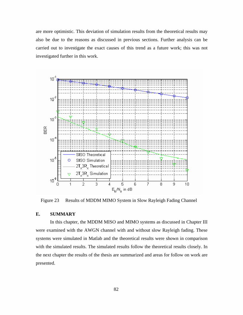
82

are more optimistic. This deviation of simulation results from the theoretical results may

also be due to the reasons as discussed in previous sections. Further analysis can be

carried out to investigate the exact causes of this trend as a future work; this was not

investigated further in this work.

Figure 23 Results of MDDM MIMO System in Slow Rayleigh Fading Channel

E. SUMMARY

In this chapter, the MDDM MISO and MIMO systems as discussed in Chapter III

were examined with the AWGN channel with and without slow Rayleigh fading. These

systems were simulated in Matlab and the theoretical results were shown in comparison

with the simulated results. The simulated results follow the theoretical results closely. In

the next chapter the results of the thesis are summarized and areas for follow on work are

presented.

83

V. CONCLUSION

The goal of this thesis was to design and analyze a MIMO system with

multicarrier delay diversity modulation. MDDM was incorporated with orthogonal

frequency division multiplexing and cyclic delay diversity. A MISO system and MIMO

systems were designed using the MDDM. They were simulated in Matlab with BPSK and

were tested in a progressive manner, first in an AWGN channel and then in a multipath

fading channel with AWGN. The BER performance of these systems was analyzed and

compared with the performance of the simulated systems. The simulated performance

results and theoretical analysis results were compared with the conventional SISO system

performance.

A. RESULTS The simulated MDDM MISO and MIMO systems achieved BER performance

results consistent with the theoretical analysis in an AWGN channel with and without

multipath fading. The performance metric of bit error probability versus 0/bE N (energy

per bit to noise power spectral density ratio) was used. To establish a fair comparison, the

transmitted power and data rate for SISO, MISO and MIMO systems were equal. The

comparison of performances in AWGN showed that the MDDM MISO system

performed better than the SISO system for low /b oE N with up to a 6.5 dB performance

gain and performed worse for higher /b oE N values. The performances of the MDDM

MIMO systems were better than that of SISO system for all values of /b oE N . MIMO

systems with two receive antennas and three receive antennas, outperformed a SISO

system by 1.7 dB and 3.4 dB performance gain. In a multipath fading channel with

AWGN, MISO and MIMO systems were able to achieve significant advantage over a

SISO system. The improvement in performances of the MDDM MISO and MIMO

systems over the SISO system can be exploited for military and civilian applications.

B. RECOMMENDATION FOR FUTURE RESEARCH There are four areas identified for future research. First, the MDDM MIMO

system performance can be analyzed in different fading conditions as described by

another fading model in place of the slow frequency nonselective Rayleigh fading

84

channel. Good choices for alternate fading models include slow Ricean frequency

nonselective fading, slow Nakagami frequency nonselective fading, and various forms of

frequency selective fading.

In addition to the analysis performed in this thesis, higher order modulation

schemes in lieu of BPSK, i.e., M PSK and M QAM, can be incorporated and analyzed to

evaluate the performance of the MDDM MIMO systems.

Next, forward error correction (FEC) coding with interleaving can be

incorporated into the MDDM MIMO system with a maximum likelihood sequence

estimation receiver. The performance can be analyzed theoretically and compared with

simulated performance.

Lastly, the MIMO system analysis herein assumes perfect CSI at the receiver. If

this information about the channel can be extracted at the receiver, then it can be sent to

the transmitter. The transmitter can use CSI to more efficiently transmit power to the

receiver through channels that are less faded than others. Techniques that control the

transmitter can be investigated and performance of the system analyzed.

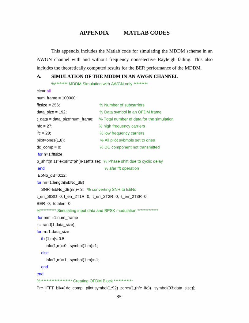
85

APPENDIX MATLAB CODES

This appendix includes the Matlab code for simulating the MDDM scheme in an

AWGN channel with and without frequency nonselective Rayleigh fading. This also

includes the theoretically computed results for the BER performance of the MDDM.

A. SIMULATION OF THE MDDM IN AN AWGN CHANNEL %******** MDDM Simulation with AWGN only ********* clear all num_frame = 100000; fftsize = 256; % Number of subcarriers data_size = 192; % Data symbol in an OFDM frame t_data = data_size*num_frame; % Total number of data for the simulation hfc = 27; % high frequency carriers lfc = 28; % low frequency carriers pilot=ones(1,8); % All pilot sybmols set to ones dc_comp = 0; % DC component not transmitted for n=1:fftsize p_shift(n,1)=exp(i*2*pi*(n-1)/fftsize); % Phase shift due to cyclic delay end % afer fft operation EbNo_dB=0:12; for nn=1:length(EbNo_dB) SNR=EbNo_dB(nn)+ 3; % converting SNR to EbNo t_err_SISO=0; t_err_2T1R=0; t_err_2T2R=0; t_err_2T3R=0; BER=0; totalerr=0; %********** Simulating input data and BPSK modulation ************* for mm =1:num_frame r = rand(1,data_size); for m=1:data_size if r(1,m)< 0.5 info(1,m)=0; symbol(1,m)=1; else info(1,m)=1; symbol(1,m)=-1; end end %******************** Creating OFDM Block ************ Pre_IFFT_blk=[ dc_comp pilot symbol(1:92) zeros(1,(hfc+lfc)) symbol(93:data_size)];

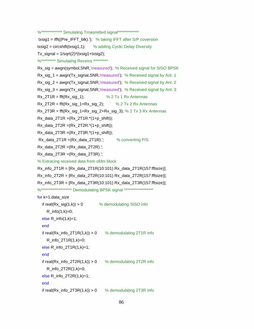
86

%************* Simulating Trnasmitted signal************* txsig1 = ifft((Pre_IFFT_blk).'); % taking IFFT after S/P coversion txsig2 = circshift(txsig1,1); % adding Cyclic Delay Diversity Tx_signal = 1/sqrt(2)*(txsig1+txsig2); %********* Simulating Receivs ********* Rx_sig = awgn(symbol,SNR,'measured'); % Received signal for SISO BPSK Rx_sig_1 = awgn(Tx_signal,SNR,'measured'); % Received signal by Ant. 1 Rx_sig_2 = awgn(Tx_signal,SNR,'measured'); % Received signal by Ant. 2 Rx_sig_3 = awgn(Tx_signal,SNR,'measured'); % Received signal by Ant. 3 Rx_2T1R = fft(Rx_sig_1); % 2 Tx 1 Rx Antennas Rx_2T2R = fft(Rx_sig_1+Rx_sig_2); % 2 Tx 2 Rx Antennas Rx_2T3R = fft(Rx_sig_1+Rx_sig_2+Rx_sig_3); % 2 Tx 3 Rx Antennas Rx_data_2T1R =(Rx_2T1R.*(1+p_shift)); Rx_data_2T2R =(Rx_2T2R.*(1+p_shift)); Rx_data_2T3R =(Rx_2T3R.*(1+p_shift)); Rx_data_2T1R =(Rx_data_2T1R).'; % converting P/S Rx_data_2T2R =(Rx_data_2T2R).'; Rx_data_2T3R =(Rx_data_2T3R).'; % Extracing received data from ofdm block Rx_info_2T1R = [Rx_data_2T1R(10:101) Rx_data_2T1R(157:fftsize)]; Rx_info_2T2R = [Rx_data_2T2R(10:101) Rx_data_2T2R(157:fftsize)]; Rx_info_2T3R = [Rx_data_2T3R(10:101) Rx_data_2T3R(157:fftsize)]; %******************* Demodulating BPSK signal ****************** for k=1:data_size if real(Rx_sig(1,k)) > 0 % demodulating SISO info R_info(1,k)=0; else R_info(1,k)=1; end if real(Rx_info_2T1R(1,k)) > 0 % demodulating 2T1R info R_info_2T1R(1,k)=0; else R_info_2T1R(1,k)=1; end if real(Rx_info_2T2R(1,k)) > 0 % demodulating 2T2R info R_info_2T2R(1,k)=0; else R_info_2T2R(1,k)=1; end if real(Rx_info_2T3R(1,k)) > 0 % demodulating 2T3R info

87

R_info_2T3R(1,k)=0; else R_info_2T3R(1,k)=1; end end %************ Probability of bit error Pb ************* err_SISO = length(find(info-R_info)); % calculating errors err_2T1R = length(find(info-R_info_2T1R)); err_2T2R = length(find(info-R_info_2T2R)); err_2T3R = length(find(info-R_info_2T3R)); t_err_SISO = t_err_SISO+err_SISO; % Calculating total errors t_err_2T1R = t_err_2T1R+err_2T1R; t_err_2T2R = t_err_2T2R+err_2T2R; t_err_2T3R = t_err_2T3R+err_2T3R; end Pb_SISO(nn) = t_err_SISO/t_data; %calculating BER Pb_2T1R(nn) = t_err_2T1R/t_data; Pb_2T2R(nn) = t_err_2T2R/t_data; Pb_2T3R(nn) = t_err_2T3R/t_data; end save MDDM_AWGN_R EbNo_dB Pb_SISO Pb_2T1R Pb_2T2R Pb_2T3R load Theo_AWGN_R figure semilogy(EbNo_dB,Pb_SISO_T,'k',EbNo_dB, Pb_2T1R_T,'r',EbNo_dB, Pb_2T2R_T,... 'b',EbNo_dB, Pb_2T3R_T,'g',EbNo_dB,Pb_SISO,'ko', EbNo_dB,Pb_2T1R,'rv',... EbNo_dB,Pb_2T2R,'b*',EbNo_dB,Pb_2T3R,'gd') grid on xlabel('E_b/N_o in dB') ylabel('P_b') legend('SISO_T','2T1R_T','2T2R_T','2T3R_T',... 'SISO_S','2T1R_S','2T2R_S','2T3R_S') title('Comparison of Theoretical and Simulated Resulsts') B. COMPUTING THEORETICAL BER OF THE MDDM IN AN AWGN

CHANNEL %******* Theoratical BER in AWGN Channel ******** clear all phase = linspace(0,2*pi*255/256,256); phi = [phase(10:101) phase(157:256)]';

88

comp = (1+cos(phi)); EbNo_dB=0:12; EbNo=10.^(EbNo_dB/10); for n = 1:length(EbNo) temp = EbNo(n); for k=1:length(phi) Q2T1R(k,n) = 0.5*erfc(sqrt(2*temp*comp(k))); Q2T2R(k,n) = 0.5*erfc(sqrt(4*temp*comp(k))); Q2T3R(k,n) = 0.5*erfc(sqrt(6*temp*comp(k))); end end %***** Theoratical BPSK ****** Pb_SISO_T=0.5*erfc(sqrt(EbNo)); Pb_2T1R_T = 1/length(phi)*sum(Q2T1R); Pb_2T2R_T = 1/length(phi)*sum(Q2T2R); Pb_2T3R_T = 1/length(phi)*sum(Q2T3R); save Theo_AWGN_R EbNo_dB Pb_SISO_T Pb_2T1R_T Pb_2T2R_T Pb_2T3R_T load MDDM_AWGN_R figure semilogy(EbNo_dB,Pb_SISO_T,'k',EbNo_dB, Pb_2T1R_T,'r',EbNo_dB,... Pb_2T2R_T,'b',EbNo_dB, Pb_2T3R_T,'g',EbNo_dB,Pb_SISO,'ko',... EbNo_dB,Pb_2T1R,'rv', EbNo_dB,Pb_2T2R,'b*',EbNo_dB,Pb_2T3R,'gd') grid on xlabel('E_b/N_o in dB') ylabel('P_b') legend('SISO_T','2T1R_T','2T2R_T','2T3R_T','SISO_S','2T1R_S','2T2R_S','2T3R_S') title('Copmarison of Theoretical and Simulated Resulsts')

C. SIMULATION OF THE MDDM IN FREQUENCY NONSELECTIVE SLOW FADING RAYLEIGH CHANNEL

%* Simulation of MDDM MISO and MIMO Systems in Frequency Nonselective Slow

% Fading Rayleigh Channel % RAYLEIGH FADING CHANNEL clear all num_frame=100000; fftsize=256; % Number of subcarriers data_size=192; % Data symbol in one frame t_data = data_size*num_frame; % Total number of data for the simulation

89

hfc = 27; % high frequency carriers lfc = 28; % low frequency carriers pilot=ones(1,8); % All pilot sybmols set to ones dc_comp = 0; % DC component not transmitted for n=1:fftsize p_shift(n,1)=exp(-i*2*pi*(n-1)/fftsize); % Phase shift due to cyclic delay end % afer fft operation EbNo_dB=0:10; for nn=1:length(EbNo_dB) SNR=EbNo_dB(nn)+3; t_err_SISO_F=0; t_err_2T1R_F=0; t_err_2T2R_F=0; t_err_2T3R_F=0; BER=0; totalerr=0; %********* Simulating input data and BPSK modulation ********* for mm =1:num_frame r=rand(1,data_size); for m=1:data_size if r(1,m)< 0.5 info(1,m)=0; symbol(1,m)=1; else info(1,m)=1; symbol(1,m)=-1; end end %******************** Creating OFDM Block ************ Pre_IFFT_blk=[ dc_comp pilot symbol(1:92) zeros(1,(hfc+lfc))... symbol(93:data_size)]; %************* Simulating Trnasmit signal************* txsig1= 1/sqrt(2)*ifft((Pre_IFFT_blk).'); % taking IFFT after S/P coversion txsig2=circshift(txsig1,1); %********* Simulating Received signal%%%%%%%%%%%%%%% % Frequency Responses of Channels h=1/sqrt(2)*(randn(1,data_size)+j*randn(1,data_size)); % SISO system channel h_11=1/sqrt(2)*(randn(1)+j*randn(1)); % Tx Ant. 1 to Rx Ant. 1 h_21=1/sqrt(2)*(randn(1)+j*randn(1)); %Freq. Response of Chan. T.A.2 to R.A.1 h_12=1/sqrt(2)*(randn(1)+j*randn(1)); %Freq. Response of Chan. T.A.1 to R.A.2 h_22=1/sqrt(2)*(randn(1)+j*randn(1)); %Freq. Response of Chan. T.A.2 to R.A.2 h_13=1/sqrt(2)*(randn(1)+j*randn(1)); %Freq. Response of Chan. T.A.1 to R.A.3 h_23=1/sqrt(2)*(randn(1)+j*randn(1)); %Freq. Response of Chan. T.A.2 to R.A.3

90

H_1=h_11+h_21*p_shift; % Composite channel response at R.A. 1 H_2=h_12+h_22*p_shift; % Composite channel response at R.A. 2 H_3=h_13+h_23*p_shift; % Composite channel response at R.A. 3 %******** Simulating Recevers ******* Rx_sig = awgn(symbol.*h,SNR,'measured'); % Received signal for SISO BPSK Rx_sig_1=awgn((txsig1*h_11+txsig2*h_21),SNR,'measured'); % simulating Ant.# 1 received signal with rayleigh flat fading channel Rx_sig_2=awgn((txsig1*h_12+txsig2*h_22),SNR,'measured'); % simulating Ant.# 2 received signal with rayleigh flat fading channel Rx_sig_3=awgn((txsig1*h_13+txsig2*h_23),SNR,'measured'); % simulating Ant.# 2 received signal with rayleigh flat fading channel fft_sig_1=fft(Rx_sig_1); fft_sig_2=fft(Rx_sig_2); fft_sig_3=fft(Rx_sig_3); %Simulating MRC Receiver Vk_SISO=Rx_sig.*conj(h); %SISO system reception with CSI Vk_1=fft_sig_1.*conj(H_1); %Antenna 1 diversity reception Vk_2=fft_sig_2.*conj(H_2); %Antenna 2 diversity reception Vk_3=fft_sig_3.*conj(H_3); %Antenna 3 diversity reception % Combining all space diversity receptions Zk_2T1R=real((Vk_1).'); %Decision variable of MISO (2T1R) and P/S conversion Zk_2T2R=real((Vk_1+Vk_2).'); %Decision variable of MIMO (2T2R) and P/S conversion Zk_2T3R=real((Vk_1+Vk_2+Vk_3).'); %Decision variable of MIMO (2T3R) and P/S conversion % Extracing real part of decision variable from ofdm block Rx_info_2T1R_F = [Zk_2T1R(10:101) Zk_2T1R(157:fftsize)]; Rx_info_2T2R_F = [Zk_2T2R(10:101) Zk_2T2R(157:fftsize)]; Rx_info_2T3R_F = [Zk_2T3R(10:101) Zk_2T3R(157:fftsize)]; Rx_info_SISO_F=real(Vk_SISO); %BPSK SISO System received data %******************* Demodulating BPSK signal ****************** for k=1:data_size if Rx_info_SISO_F(1,k) > 0 % demodulating SISO info R_info_SISO_F(1,k)=0; else R_info_SISO_F(1,k)=1; end if Rx_info_2T1R_F(1,k) > 0 % demodulating 2T1R info R_info_2T1R_F(1,k)=0; else R_info_2T1R_F(1,k)=1;

91

end if Rx_info_2T2R_F(1,k) > 0 % demodulating 2T2R info R_info_2T2R_F(1,k)=0; else R_info_2T2R_F(1,k)=1; end if Rx_info_2T3R_F(1,k) > 0 % demodulating 2T3R info R_info_2T3R_F(1,k)=0; else R_info_2T3R_F(1,k)=1; end end %%************ Probability of bit error Pb ************* err_SISO_F = length(find(info-R_info_SISO_F)); % calculating errors err_2T1R_F = length(find(info-R_info_2T1R_F)); err_2T2R_F = length(find(info-R_info_2T2R_F)); err_2T3R_F = length(find(info-R_info_2T3R_F)); t_err_SISO_F = t_err_SISO_F+err_SISO_F; % Calculating total errors t_err_2T1R_F = t_err_2T1R_F+err_2T1R_F; t_err_2T2R_F = t_err_2T2R_F+err_2T2R_F; t_err_2T3R_F = t_err_2T3R_F+err_2T3R_F; end Pb_SISO_F(nn) = t_err_SISO_F/t_data; %calculating BER Pb_2T1R_F(nn) = t_err_2T1R_F/t_data; Pb_2T2R_F(nn) = t_err_2T2R_F/t_data; Pb_2T3R_F(nn) = t_err_2T3R_F/t_data; end save MDDM_SRF_R EbNo_dB Pb_SISO_F Pb_2T1R_F Pb_2T2R_F Pb_2T3R_F load Theo_SRF_R figure semilogy(EbNo_dB,Pb_SISO_F_T,'k',EbNo_dB, Pb_2T1R_F_T,'r',EbNo_dB,... Pb_2T2R_F_T,'b',EbNo_dB, Pb_2T3R_F_T,'g',EbNo_dB,Pb_SISO_F,'ko',... EbNo_dB,Pb_2T1R_F,'rv', EbNo_dB,Pb_2T2R_F,'b*',EbNo_dB,Pb_2T3R_F,'gd') grid on xlabel('E_b/N_o in dB') ylabel('P_b') legend('SISO_T','2T1R_T','2T2R_T','2T3R_T','SISO_S','2T1R_S','2T2R_S','2T3R_S') title('Copmarison of Theoretical and Simulated Resulsts')

92

D. COMPUTING THEORETICAL BER OF THE MDDM IN FREQUENCY NONSLECECTIVE SLOW FADING RAYLEIGH CHANNEL

% Calculating Theoretical Results By Numerical Methods global W X N EbNo_dB = 0:10; EbNo = 10.^(EbNo_dB/10); % creating independent channel responses h_11=1/sqrt(2)*(randn(1,10^6)+j*randn(1,10^6)); % Tx Ant. 1 to Rx Ant.1 h_21=1/sqrt(2)*(randn(1,10^6)+j*randn(1,10^6)); % T.A.2 to R.A.1 h_12=1/sqrt(2)*(randn(1,10^6)+j*randn(1,10^6)); % T.A.1 to R.A.2 h_22=1/sqrt(2)*(randn(1,10^6)+j*randn(1,10^6)); % T.A.2 to R.A.2 h_13=1/sqrt(2)*(randn(1,10^6)+j*randn(1,10^6)); % T.A.1 to R.A.3 h_23=1/sqrt(2)*(randn(1,10^6)+j*randn(1,10^6)); % T.A.2 to R.A.3 H_1=h_11+h_21; %*p_shift; % Effective hannel response at R.A. 1 H_2=h_12+h_22; %*p_shift; % Effective channel response at R.A. 2 H_3=h_13+h_23; %*p_shift; % Effective channel response at R.A. 3 % creating random variables Beta Beta_1=((H_1).*conj(H_1)); Beta_2=((H_1).*conj(H_1))+((H_2).*conj(H_2)); Beta_3=((H_1).*conj(H_1))+((H_2).*conj(H_2))+((H_3).*conj(H_3)); [N1 X1]=hist(Beta_1,500); [N2 X2]=hist(Beta_2,500); [N3 X3]=hist(Beta_3,500); % Theoretical BER foR SISO x = sqrt(2*EbNo./(1+2*EbNo)); Pb_SISO_F_T = 0.5*(1-x); % Estimating PDF Beta_1 and Calculting Theoretical BER for 2T1R X=X1; N=N1; W=quad(@Func_Est_Cur,min(X1),max(X1)); % Normalizing factor for PDF Pr_Beta_1 = quad(@Func_pdf_Beta,min(X1), max(X1)) dBeta_1=(min(X1):0.0001:max(X1)); for i=1:length(EbNo) Q_2Beta_1 = 0.5*erfc(sqrt(2*EbNo(i)*dBeta_1)); Pb_2T1R_F_T(i) = sum(Q_2Beta_1.*abs(Func_pdf_Beta(dBeta_1)))*0.0001; end % Estimating PDF Beta_2 and Calculting Theoretical BER for 2T2R X=X2; N=N2;

93

W=quad(@Func_Est_Cur,min(X2),max(X2)); % Normalizing factor for PDF Pr_Beta_2 = quad(@Func_pdf_Beta,min(X2), max(X2)) dBeta_2=(0:0.0001:max(X2)); for i=1:length(EbNo) Q_2Beta_2 = 0.5*erfc(sqrt(2*EbNo(i)*dBeta_2)); Pb_2T2R_F_T(i) = sum(Q_2Beta_2.*abs(Func_pdf_Beta(dBeta_2)))*0.0001; end % Estimating PDF Beta_3 and Calculting Theoretical BER for 2T3R X=X3; N=N3; W=quad(@Func_Est_Cur,min(X3),max(X3)); % Normalizing factor for PDF Pr_Beta_3 = quad(@Func_pdf_Beta,min(X3), max(X3)) dBeta_3=(0:0.0001:max(X3)); for i=1:length(EbNo) Q_2Beta_3 = 0.5*erfc(sqrt(2*EbNo(i)*dBeta_3)); Pb_2T3R_F_T(i) = sum(Q_2Beta_3.*abs(Func_pdf_Beta(dBeta_3)))*0.0001; end save Theo_SRF_R EbNo_dB Pb_SISO_F_T Pb_2T1R_F_T Pb_2T2R_F_T Pb_2T3R_F_T load MDDM_SRF_R figure semilogy(EbNo_dB,Pb_SISO_F_T,'k',EbNo_dB, Pb_2T1R_F_T,'r',EbNo_dB, ... Pb_2T2R_F_T,'b',EbNo_dB, Pb_2T3R_F_T,'g',EbNo_dB,Pb_SISO_F,'ko',... EbNo_dB,Pb_2T1R_F,'rv', EbNo_dB,Pb_2T2R_F,'b*',EbNo_dB,Pb_2T3R_F,'gd') grid on xlabel('E_b/N_o in dB') ylabel('P_b') legend('SISO_T','2T1R_T','2T2R_T','2T3R_T','SISO_S','2T1R_S','2T2R_S','2T3R_S') title('Comparison of Theoretical and Simulated Resulsts') E. FUNCTIONS TO INTERPOLATE PROBABAILITY DISTRIBUTION

FUNCTIONS function y = Func_Est_Cur(x); %Title : Estimation of Data Distribution of Random Variable Beeta %Author : Muhammad Shahid, Naval Post Graduate School, Septermber 2005 %----------------------------------------------------------------------- % y = Func_Est_Cur(x) %----------------------------------------------------------------------- %Input : Random variabel Beeta %Output : Estimated Data Distribution of Beeta

94

%----------------------------------------------------------------------- global W X N y=spline(X,N,x);

function PDF = Func_pdf_Beta(b_2); %Title : Interoplation of PDF of Random Variable Beeta %Author : Muhammad Shahid, Naval Post Graduate School, Septermber 2005 %----------------------------------------------------------------------- % PDF = Func_pdf_Beta(b_2); %----------------------------------------------------------------------- %Input : Random variabel Beeta %Output : PDF of Beeta %----------------------------------------------------------------------- global W X N PDF=spline(X,N,b_2)/W;

95

LIST OF REFERENCES

[1] Branka Vucetic and Jinhong Yuan, “Space-Time Coding.” John Wiley & Sons,

West Sussex, England, 2003.

[2] Jun Tan, Gordon L. Stuber, “Multicarrier Delay Diversity Modulation for OFDM

Systems.” IEEE Transactions on Wireless Communications, Vol. 3, No. 5,

September 2004. pp. 1756-1763.

[3] A. Wittneben, “A new bandwidth efficient transmit antenna modulation diversity

scheme for linear digital modulation.” in Proc. IEEE Int. Conf. Communications,

1993, pp. 1630-1634.

[4] N. Seshadri and J. H. Winters, “Two signaling schemes for improving the error

performance of frequency-division-duplex (FDD) transmission systems using

transmitter antenna diversity.” Int J. Wireless Inform. Networks, vol. 1, No. 1, pp.

24-47, January 1994.

[5] S. Kaiser, “Spatial transmit diversity techniques for broadband OFDM systems.”

in Proc. IEEE GLOBECOM, San Francisco, California, November 2000, pp.

1824-1828.

[6] A. Dammann and S. Kaiser, “Standard conformable antenna diversity techniques

for OFDM and its application to the DVB-T system.” in Proc. IEEE

GLOBECOM, San Antonio, Texas, November 2001, pp. 3100-3105.

[7] A. Paulraj, R. Nabar and D. Gore, “Introduction to Space Time Wireless

Communications.” Cambridge University Press, Cambridge, United Kingdom,

2003.

[8] Michael J. Turpin, “An Investigation of a Multiple-Input Multiple-Output

Communication System with the Alamouti Space-Time Code.” Master’s Thesis,

Naval Postgraduate School, Monterey, California, June 2004.

96

[9] Erwin Kreyszig, “Advanced Engineering Mathematics, Fourth Edition.” John

Wiley & Sons, New York, 1979.

[10] Bernard Sklar, “Digital Communications Fundamentals and Applications.”

Second Edition, Prentice Hall, Upper Saddle River, New Jersey, 2002.

[11] Meixia Tao and Toger S. Cheng, “Spade Code Design in Delay Diversity

Transmission for PSK modulation.” Vehicular Technology Conference, 2002.

Proceedings. IEEE 56th Volume 1, 24-28 Sept. 2002, pp. 444-448, vol. 1.

[12] Gerhaud Bauch and Javed Shamim Malik, “Orthogonal Frequency Division

Multiple Access with Cyclic Delay Diversity.” ITG Workshop on Smart

Antennas, 2004, pp. 17-24.

[13] Roberto Cristi, “Modern Digital Signal Processing.” Brooks/Cole-Thomson

Learning, Pacific Grove, California USA, 2004.

[14] Patrick A. Count, “Performance Analysis of OFDM in Frequency Selective,

Slowly Fading Nakaghami Channel.” Master’s Thesis, Naval Postgraduate

School, Monterey, California, June 2001.

[15] Clark Robertson, “EC4550 Digital Communications Systems Lecture Notes.”

Naval Postgraduate School, Monterey, California 2004 (unpublished).

[16] John G. Proakis, “Digital Communications.” Fourth Edition, McGraw Hill, New

York, 2001.

[17] Theodore S. Rappaport, “Wireless Communications Principles and Practice.”

Second Edition, Prentice Hall PTR, Upper Saddle River, New Jersey, 2002.

[18] Charles W. Therrien, Murali Tummala, “Probability for Electrical and Computer

Engineers.” CRC Press, Washington, D.C. 2004.

[19] Peyton Z. Peebles Jr., “Probability, Random Variables and Random Signal

Principles.” Fourth Edition, McGraw-Hill, New York, 2001.

97

[20] Halil Derya Saglam, “Simulation Performance of Multiple-input Multiple-output

System Employing Single-carrier Modulation and Orthogonal Frequency Division

Multiplexing.” Master’s Thesis, Naval Postgraduate School, Monterey,

California, December 2004.

[21] Matlab Helpfile, The Math Works, Inc., Version 7.0.4.365 (R14) Service Pack 2,

Nathic, Massachusetts, 29 January 2005.

[22] Fredrik Kristensen, Peter Nilson and Anders Olsson, “A Generic Transmitter for

Wireless OFDM Transmitter.” The 14th IEEE 2003 International Symposium on

Personal, Indoor and Mobile Radio Communication Proceedings.

[23] IEEE Std. 802.16-2001, IEEE Standard for Local and Metropolitan area networks

Part 16: Air Interface for Fixed Broadband Wireless Access Systems.

98


99

INITIAL DISTRIBUTION LIST

1. Defense Technical Information Center Ft. Belvoir, Virginia

2. Dudley Knox Library Naval Postgraduate School Monterey, California

3. Chairman, Code EC Electrical and Computer Engineering Department Naval Postgraduate School Monterey, California

4. Frank Kragh, Code EC/Kh Electrical and Computer Engineering Department Naval Postgraduate School Monterey, California

5. Tri Ha, Code EC/Ha

Electrical and Computer Engineering Department Naval Postgraduate School Monterey, California

6. Clark Robertson, Code EC/Rc

Electrical and Computer Engineering Department Naval Postgraduate School Monterey, California

7. Muhammad Shahid Pakistan Air Force

Documents

A 439819