Embed Size (px)
Citation preview
ESTIMATES OF DIABATIC WIND SPEED PROFILES FROM
NEAR-SURFACE WEATHER OBSERVATIONS
A. A. M. HOLTSLAG
Royal Netherlands Meteorological Institute, De Bilt, The Netherlands
(Received in final form 27 March, 1984)
Abstract. In this paper we analyse diabatic wind profiles observed at the 213 m meteorological tower at Cabauw, the Netherlands. It is shown that the wind speed profiles agree with the well-known similarity functions of the atmospheric surface layer, when we substitute an effective roughness length. For very unstable conditions, the agreement is good up to at least 200 m or z/L u - 7 (z is height, L is Obukhov length scale). For stable conditions, the agreement is good up to z/L N 1. For stronger stability, a semi-empirical extension is given of the log-linear profile, which gives acceptable estimates up to u 100 m. A scheme is used for the derivation of the Obukhov length scale from single wind speed, total cloud cover and air temperature. With the latter scheme and the similarity functions, wind speed profiles can be estimated from near-surface weather data only. The results for wind speed depend on height and stability. Up to 80 m, the rms difference with observations u is on average u 1.1 m s - ‘. At 200 m, u = 0.8 m s - ’ for very unstable conditions increasing to c N 2.1 m s - i for very stable conditions. The proposed methods simulate the diurnal variation of the 80 m wind speed very well. Also the simulated frequency distribution of the 80 m wind speed agrees well with the observed one. It is concluded that the proposed methods are applicable up to at least 100 m in generally level terrain.
1. Introduction
Knowledge of the mean wind profile is of importance for, e.g., air pollution and wind energy studies. In practice, however, only surface weather observations such as 10 m wind speed are available most of the time. In such cases, there is a need for the description of the mean wind speed with height as some function of the available data.
During adiabatic (neutral) conditions, the variation of mean wind speed with height is well described by a logarithmic relationship. This relationship has been found to satisfy observations’in the lower atmosphere up to 100 m or more (e.g., Lumley and Panofsky, 1964; Tennekes, 1982). In diabatic conditions, however, when the surface heat flux is significantly different from zero, stability corrections should be made to the logarithmic relationship. These stability corrections are important, for instance, for the correct simulation of the diurnal variation of wind speed. Also the frequency distribution of wind speed is affected by stability.
The stability corrections may result from the application of Monin-Obukhov simi- larity theory for the atmospheric surface layer (Monin and Yaglom, 1971). With the latter theory, we can obtain flux-profile relationships for the surface layer. In the past two decades, much research has been done on these relationships in diabatic conditions above homogeneous terrain. A review of the relations is given by Dyer (1974) and Yaglom (1977).
With the flux-profile relationships, we can obtain the diabatic wind speed profile using a single wind speed observation, the surface roughness length and the so-called Obukhov
Boundary-Layer Meteorology 29 (1984) 225-250. OOOS-8314/84/0293-0225$03.90. 0 1984 by D. Reidel Publishing Company.
226 A. A. M. HOLTSLAG
length scale (see Section 2). Problems may arise, however, when the relations are applied for terrain with upwind inhomogenities. In such cases, an effective roughness length is appropriate (Fiedler and Panofsky, 1972). This is demonstrated recently by Korrell et al. (1982) and Beljaars (1982). A recent discussion on surface-layer similarity under non-uniform fetch conditions is given by Beljaars et al. (1983).
In this paper, we analyse the use of the Monin-Obukhov similarity functions for practical applications in generally level terrain. For that reason, the observations of diabatic wind profiles up to 200 m at the Cabauw tower are analysed in the first part of the paper. We investigate the utility of similarity functions proposed in the literature, together with the effective roughness length concept. For analysis of the wind profiles, we use the Obukhov length scale derived from profiles of wind and temperature near the surface (profile method).
For practical application of the similarity functions, however, routine estimates of the Obukhov length scale and the effective surface roughness length are needed. Recently, routine procedures for the derivation of the Obukhov length scale from near-surface weather data were given by Holtslag and Van Ulden (1982, 1983). Moreover, Wieringa (1976, 1980) has provided a routine method for derivation of the effective surface roughness length for generally level terrain.
In the second part of the paper, we shall demonstrate the skill of the above methods for the routine application of the Monin-Obukhov similarity functions. For that purpose, observations of 10 m wind speed, air temperature and total cloud cover or insolation are needed. As such, the methods can replace empirical power ‘laws’, the use of which has no physical foundation and only little practical advantage (Wieringa, 198 1). More- over, the methods can serve for a mesoscale analysis of surface layer wind, with procedures discussed by Cats (1980).
2. Background
2.1. MONIN-OBUKHOV SIMILARITY THEORY
The mean wind profile in the atmospheric surface layer can be described according to Monin-Obukhov similarity theory. First the Obukhov length scale L is defined as (Monin and Yaglom, 1971; Tennekes, 1982)
L=-u3. k g wT
T
(1)
Here u* is the friction velocity, k the Von Karman constant, g/T the buoyancy parameter -.
(g accelaration of gravity, T air temperature) and wT is related to the sensible heat flux H by -
H = pC,wT, (2)
where p is the density of air and C, is specific heat at constant pressure.
DIABATIC WIND PROFILES 221
The Monin-Obukhov theory is based on the hypothesis that the non-dimensional wind gradient can be written as
(3)
where $J~ is a function of z/L only. Here Uis the mean wind speed at the height z. Several forms of & have been proposed for unstable conditions (L < 0). We will investigate
&, = (1 - 16 z/L)- 1’4, (44
as reviewed by Dyer (1974) and proposed by Hicks (1976) for - 2 I z/L I 0. Also
c& = (1 - 16 z/L)- 1’3, t4b)
as given by Carl et al. (1973) for - 10 I z/L I - 1 is investigated. The latter formulation agrees well with the well known KEYPS form and approaches the free convection limit for z/L -+ - co (Lumley and Panofsky, 1964).
For stable conditions (L > 0), the result for &, is usually written as
where a is a coefficient. Dyer (1974) proposes a = 5 for moderate stable conditions. This is confirmed by Webb (1970), SethuRaman and Brown (1976) and Hicks (1976). But the latter authors indicate that &,, is different for stronger stabilities. This subject is discussed in more detail in Section 6.
In Equations (4a)-(4c), the corresponding value of the Von Karman constant is given by k = 0.41.
2.2. INTEGRAL WIND PROFILES
The wind speed profile is obtained from the integration of (3) between the surface and a height z in the surface layer, which results in
where U, is wind speed at height z, z,, is the appropriate surface roughness lenght and $M is defined by
(6)
228 A. A. M. HOLTSLAG
In this paper, we assume that a wind speed U, is available at one level zi in the surface layer. In that case, (5) can be rewritten as
(7)
With the aid of (7), U, is obtained at z, for given U,, z0 and L. The direction of U, is assumed to be the same as the direction of U,. This subject is verified with our data in Section 5.
Finally (6) is applied to Equations (4a)-(4c). Application to (4a) leads to (Paulson, 1970)
where x = $& ‘. When (6) is applied to (4b) we obtain
2x+ 1 ljM+n(x2+x+ 1)-&r-’ ~ ( > $
-sIn3 +$/3
where again X = $J; ‘, but here $,,, is given by (4b). Application of (6) to (4~) gives
In this paper, we shall use (8a) and (8b) in their quite complex form. For simple practical applications, we can obtain approximations in the form of simple polynomials in z/L fitted to (8a) and (8b) by least-square methods. Use of the simpler forms of the equations for tiM results in significant savings of computer time with some loss of accuracy (see Schultz, 1979).
2.3. THE EFFECTIVE SURFACE ROUGHNESS LENGTH
In the integral profiles (5) and (7), the surface roughness length is apparent. This surface roughness length may differ from the local roughness length of the terrain due to inhomogenities of the surface in the upwind direction. The upwind inhomogenities may occur due to occasional obstructions in a relatively smooth field or due to large pertur- bations. In both cases an efictive roughness length (Fiedler and Panofsky, 1972) was found appropriate for use in the flux-profile relationship (5). This is discussed by Beljaars (1982) for near-neutral profiles at Cabauw. Korrell et al. (1982) showed the usefulness of an effective roughness length for the description of wind data obtained at the Boulder tower (40” N, 105” W).
In the above, the effective surface roughness length is defined as the roughness length
DIABATIC WIND PROFILES 229
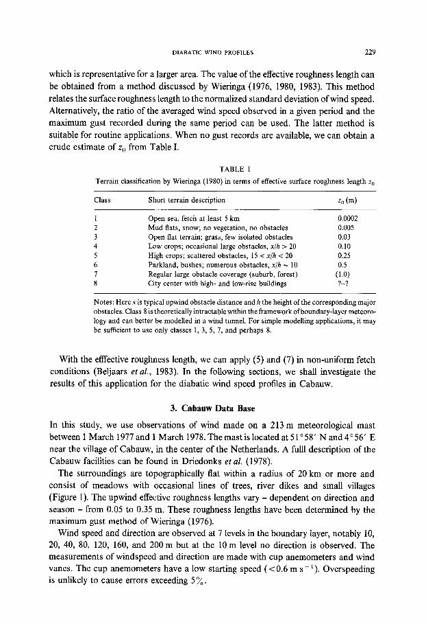
which is representative for a larger area. The value of the effective roughness length can be obtained from a method discussed by Wieringa (1976, 1980, 1983). This method relates the surface roughness length to the normalized standard deviation of wind speed. Alternatively, the ratio of the averaged wind speed observed in a given period and the maximum gust recorded during the same period can be used. The latter method is suitable for routine applications. When no gust records are available, we can obtain a crude estimate of z,, from Table I.
TABLE I
Terrain classification by Wieringa (1980) in terms of effective surface roughness length a,,
Class Short terrain description z. Cm)
Open sea, fetch at least 5 km 0.0002 Mud flats, snow; no vegetation, no obstacles 0.005 Open flat terrain; grass, few isolated obstacles 0.03 Low crops; occasional large obstacles, x/h > 20 0.10 High crops; scattered obstacles, 15 i x/h < 20 0.25 Parkland, bushes; numerous obstacles, x/h - 10 0.5 Regular large obstacle coverage (suburb, forest) (1.0) City center with high- and low-rise buildings ?-?
Notes: Here x is typical upwind obstacle distance and h the height of the corresponding major obstacles. Class 8 is theoretically intractable within the framework ofboundary-layer meteoro- logy and can better be modelled in a wind tunnel. For simple modelling applications, it may be sufficient to use only classes 1, 3, 5, 7, and perhaps 8.
With the ellfective roughness length, we can apply (5) and (7) in non-uniform fetch conditions (Beljaars et al., 1983). In the following sections, we shall investigate the results of this application for the diabatic wind speed profiles in Cabauw.
3. Cabauw Data Base
In this study, we use observations of wind made on a 213 m meteorological mast between 1 March 1977 and 1 March 1978. The mast is located at 5 lo 58’ N and 4” 56’ E near the village of Cabauw, in the center of the Netherlands. A full1 description of the Cabauw facilities can be found in Driedonks et al. (1978).
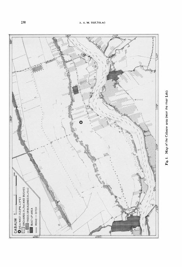
The surroundings are topographically flat within a radius of 20 km or more and consist of meadows with occasional lines of trees, river dikes and small villages (Figure 1). The upwind effective roughness lengths vary - dependent on direction and season - from 0.05 to 0.35 m. These roughness lengths have been determined by the maximum gust method of Wieringa (1976).
Wind speed and direction are observed at 7 levels in the boundary layer, notably 10, 20, 40, 80, 120, 160, and 200 m but at the 10 m level no direction is observed. The measurements of windspeed and direction are made with cup anemometers and wind vanes. The cup anemometers have a low starting speed (x0.6 m s- ‘). Overspeeding is unlikely to cause errors exceeding 5%.
230 A. A. M. HOLTSLAG
DIABATIC WIND PROFILES 231
The wind instruments are mounted 0.5 m above a boom which extends 9.4 m beyond the mast. Originally it was believed that this construction restricted the interference of the mast on the wind measurements within 1 y0 (Gill et al., 1967). However, a preliminary analysis shows that for some wind directions, the error due to obstruction by booms and tower is much larger (Wessels, 1983). Therefore, in this paper two wind direction categories were selected for which the above systematic error is less than - 2%. The two categories are South-East (direction between 60 and 200 deg) and North-West (between 280 and 340 deg).
Within the selected two wind direction categories, we have chosen data for which no instrumental or observational errors were reported and for which no rain, snow or fog appeared. We used 30 min averages of each second half hour for which 10 m windspeed U,, 2 1 m s - l. The second half hour was used because in that half hour, observations of total cloud cover were present at four nearby meteorological stations. The total cloud cover was taken as the average of the four values. Further, the observed temperature in Cabauw at 2 m was used. The latter height agrees with the height of routine temperature observation. For the derivation of the Obukhov length with the profile method, the observed temperature difference between 10 and 0.6 m was used (see Section 4).
After the above data selection, 1277 half hourly runs were retained for the South-East sector and 328 runs for the North-West sector. As will be shown below, the selected runs represent a broad range of stability conditions. Because of the selection, however, the data set is not representative for the wind climate in Cabauw. This is caused in particular by the deletion of South-West winds, in which high speeds are often observed. In such cases, however, the stability correction is small, just as in cases with precipitation or fog. The value of the present analysis, therefore, is not affected by the above data selection.
4. Derivation of the Obukhov Length Scale
As discussed in Section 2, the ratio z/L between the height z and the Obukhov length scale L determines the stability correction in the wind profiles. The parameter L can be obtained from delicate turbulence measurements, but such measurements are scarce in practice. In this section we discuss, therefore, two methods for the derivation of L from the available data. In fact, both methods provide the surface fluxes of heat and momentum. Then L is easily obtained from (1).
The first method is the profile method in which the fluxes are obtained from the profiles of wind and temperature near the surface (McBean, 1979; Berkowitz and Prahm, 1982; Holtslag and Van Ulden, 1983). From integration of (3) between the appropriate surface roughness length .q, and a height in the surface layer z, we obtain (Paulson, 1970)
(9)

232 A. A. M. HOLTSLAG
where $M is given by (8a) for unstable conditions and (8~) for stable conditions. The equivalent for the temperature profile is (Paulson, 1970):
where A0 is a given temperature difference between two heights z, and z,. The function I&, is given by
ll;I = 21n 5 , ( >
(11)
for unstable conditions (L < 0). Here y = $; ‘, where &, is the counterpart of (3) for the temperature profile. As proposed by Dyer (1974), we take A = $2 for unstable conditions with & given by (4a). In stable conditions, we assume $,, = em as supported by Webb (1970) and Hicks (1976) for values of z/L 6 1. This results in $H = I,& where $,,,, is given by (8~) with a = 5. The temperature scale & of (10) is related to the friction velocity u* and the sensible heat flux H by
H= -pc,udh. (12)
From (9) and (10) u* and &I can be obtained starting with a prescribed value of the Obukhov length scale L. We have used L = co (e.g., IG;I = I& = 0). First estimates of u* and I% are then computed. With these values, L is computed using (l), (2), and (12). Subsequently, the new value of L is substituted in (9) and (10) to obtain improved estimates for u* and I%. This cycle is repeated until successive values of L do not change more than 5 %. It appears that not more than three iteration steps are needed in most cases to achieve the required accuracy for L. It must be noted that for stable conditions, the above set of equations can also be solved analytically.
The above method for the derivation of L uses a single windspeed U, , the effective surface roughness length z,,, air temperature T and a temperature difference Aenear the surface. With this method, estimates of L are obtained which agree with those from scarce turbulence measurements (Nieuwstadt, 1978; Beljaars, 1982). For that reason, this method is used for the analysis of the Cabauw wind profiles in Section 5. We have used 30 min averages of the locally observed 10 m wind speed and the observed temperature difference between z, = 10 m and zi = 0.6 m.
For routine applications, however, the above method is not suitable in most cases, because often the temperature difference A0 is not available. In such cases we must parameterize the sensible heat flux (12). De Bruin and Holtslag (1982) and Holtslag and Van Ulden (1982, 1983) have given procedures for the derivation of the sensible heat flux from routine weather data only. Afterwards, L is obtained from (1) and (9). In the appendix a summary of the parameterization of L is given. It appears that the estimates of L with the latter scheme are in good agreement with values of L obtained from the profile method. In Sections 7 and 8, the usefulness of the routine method is demon- strated for the derivation of wind profiles.
DIABATIC WIND PROFILES 233
With the above profile and routine method for the derivation of L, no reliable solutions exist for stable conditions in which the Richardson number Ri = (z/L)/(l + 5 z/L) approaches the critical value of 0.20. This appears in very stable conditions, in which the transfer by turbulence is small. Moreover, we have assumed &, = em, but in extremely stable conditions Hicks (1976) obtained $I,, N 2 &. The latter means that the transfer mechanism for heat is smaller than for momentum. For that reason, the application of the two methods is restricted to cases with z/L I 1. The value z/L = 1 results in Ri = 0.167, which is close to the critical value of 0.20, For z/L 2 1, the fluxes are small and difficult to determine (e.g., Carson and Richards, 1978). A simple practical solution for L in these conditions is discussed in the Appendix. The consequences for the stable wind profile are treated in Section 6.
5. Wind Profile Analysis
In this section we analyse the observed wind profiles at Cabauw in terms of the Monin-Obukhov theory described in Section 2. To show the influence of stability on wind profiles up to 200 m, we have distinguished 9 classes of stability. These classes range from very unstable (a) to very stable (i). The classes were defined with the use of the Obukhov length scale derived with the profile method (Table II). The relation of these classes with the other categories of Table II is discussed below. For each class -- and height z, wind ratios of (UJ U,,) and (UJU,,) were determined. The difference was found negligible as in Korrell et al. (1982). This means that a, may be plotted as a function of z to show the influence of stability in each class. Moreover in each class a central value of L can be given with L, = 1/(1/L).
Figure 2 shows the observed mean wind speed profiles for 4 classes of stability ranging from neutral to unstable conditions. In the figure, we have used all available data of the South-East wind category between 1 May and 1 September (summer months) with
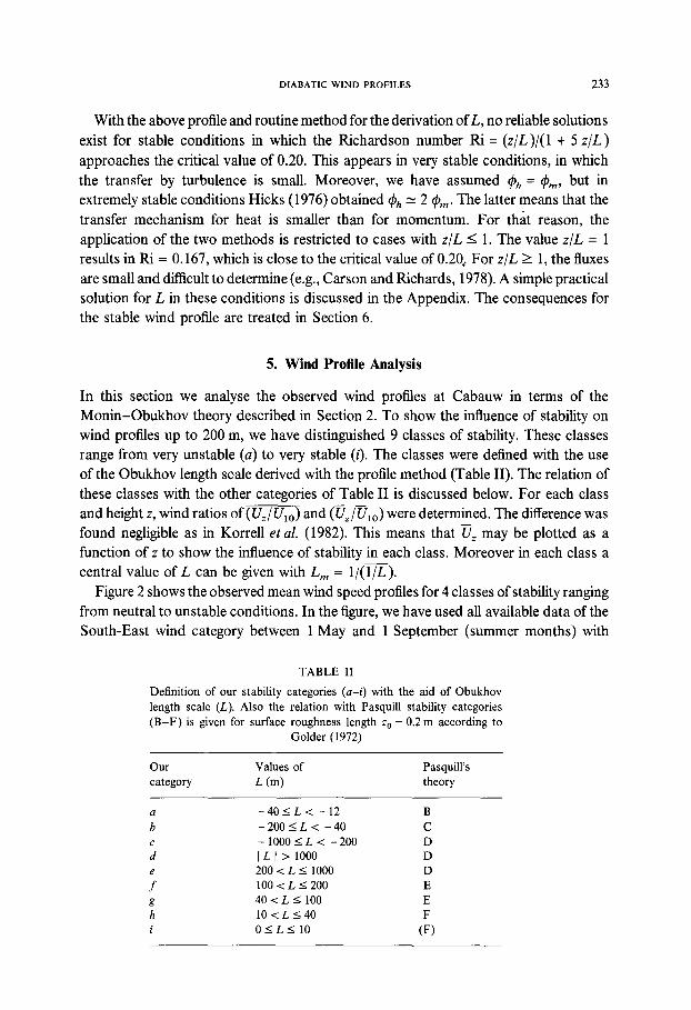
TABLE II
Definition of our stability categories (u-i) with the aid of Obukhov length scale (L). Also the relation with Pasquill stability categories (B-F) is given for surface roughness length z0 = 0.2 m according to
Golder (1972)
Our category
Values of Pasquill’s L (m) theory
-4OILi -12 -2OOSL< -40 -lOOOSL< -200 11 L (1 > 1000 200 <L I 1000 100<L~200 4O<LS 100 lO<L140 OSL<lO
B C D D D E E
CL
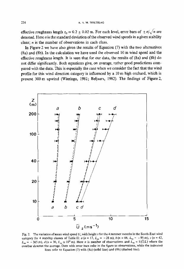
234 A. A. M. HOLTSLAG
effective roughness length z,, N 0.2 + 0.02 m. For each level, error bars of 4 G/,/% are denoted. Here ais the standard deviation of the observed wind speeds in a given stability class; n is the number of observations in each class.
In Figure 2 we have also given the results of Equation (7) with the two alternatives @a) and (8b). In the calculation we have used the observed 10 m wind speed and the effective roughness length. It is seen that for our data, the results of (8a) and (8b) do not differ significantly. Both equations give, on average, rather good predictions com- pared with the data. This is especially the case when we consider the fact that the wind profile for this wind direction category is influenced by a 10 m high orchard, which is present 300 m upwind (Wieringa, 1981; Beljaars, 1982). The findings of Figure 2,
A 200
100
40
20
10
I
/ -
1 -
0 -
b C C d d
b cd
5 10
u ,(l?ls-'1
l! 5
Fig. 2. The variation ofmean wind speed U, with height z for the 4 summer months in the South-East wind category for 4 stability classes of Table II: a (n = 17, L, = -28m),b(n=66,L,= -95m),c(n=42, - L, = - 365 m), d (n = 30, L, N lo4 m). Here n is number of observations and L, = 1/(1/L) where the overbar denotes the average. Dots with error bars refer in the figure to observations, while the indicated
lines refer to Equation (7) with (8a) (solid line) and (8b) (dashed line).
DIABATIC WIND PROFILES 235
therefore, support the use of an effective roughness length together with stability information.
In the paper by Carl et al. (1973) the utility of the @m functions given by (4a) and (4b) is discussed. They conclude that (4b) shows good agreement with their data up to z/ -L N 10, while (4a) fits better for small z/ -L. The integral forms of (4a) and (4b), however, do not differ signifkantly (Figure 2). In the unstable class a, we obtain with our data that both integral functions (8a) and (8b) are applicable up to at least 200 m or z/ -L N 7, on average.
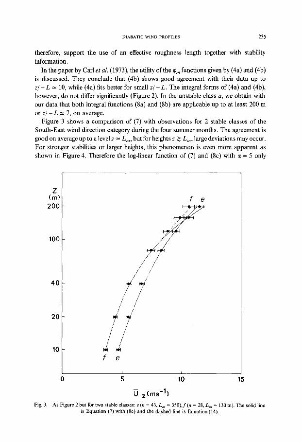
Figure 3 shows a comparison of (7) with observations for 2 stable classes of the South-East wind direction category during the four summer months. The agreement is good on average up to a level z N L,, but for heights z 2 L,, large deviations may occur. For stronger stabilities or larger heights, this phenomenon is even more apparent as shown in Figure 4. Therefore the log-linear function of (7) and (8~) with a = 5 only
A 200
100
40
20
0
f e
15
Fig. 3. As Figure 2 but for two stable classes: e (n = 43, L, = 350),f(n = 28, L, = 130 m). The solid line is Equation (7) with (8~) and the dashed line is Equation (14).
236 A. A. M. HOLTSLAG
(5 200
100
40
20
10
ihg
0 5 10 15
cl z( t?ld)
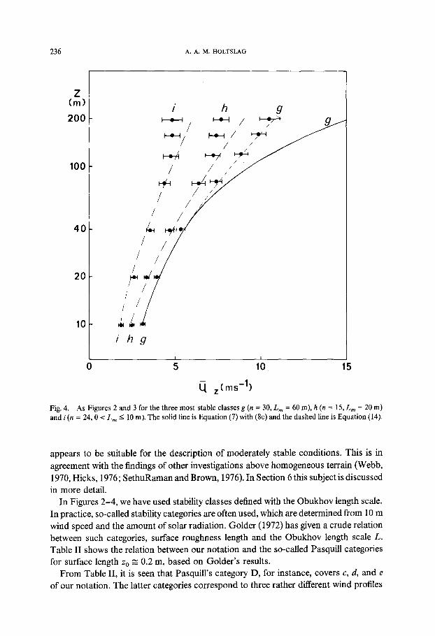
Fig. 4. As Figures 2 and 3 for the three most stable classes g (n = 30, L, = 60 m), h (n = 15, L, = 20 m) and i (n = 24,0 < L, I 10 m). The solid line is Equation (7) with (8~) and the dashed line is Equation (14).
appears to be suitable for the description of moderately stable conditions. This is in agreement with the findings of other investigations above homogeneous terrain (Webb, 1970, Hicks, 1976; SethuRaman and Brown, 1976). In Section 6 this subject is discussed in more detail.
In Figures 2-4, we have used stability classes defined with the Obukhov length scale. In practice, so-called stability categories are often used, which are determined from 10 m wind speed and the amount of solar radiation. Golder (1972) has given a crude relation between such categories, surface roughness length and the Obukhov length scale L. Table II shows the relation between our notation and the so-called Pasquill categories for surface length z, g 0.2 m, based on Golder’s results.
From Table II, it is seen that Pasquill’s category D, for instance, covers c, d, and e of our notation. The latter categories correspond to three rather different wind profiles
DIABATIC WIND PROFILES 231
as shown in Figures 2 and 3. This result is also obtained when UJU,, is used as the independent variable in the figures instead of U, (not shown here). Significant stability variations can be found within a single stability category of Pasquill, especially at larger heights. This shows that in fact z/L is the proper stability parameter for wind profiles. This is one of the reasons why the use of power ‘laws’ related to broad stability categories should be avoided. A discussion on this subject is given by Wieringa (1981).
Finally, we discuss the influence of change in wind direction. In the above we have assumed implicity, that the direction of U, is given by the direction of the 10 m wind
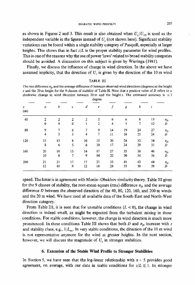
TABLE III
The rms difference uD and the average difference D between observed wind directions (degrees) at the height z and the 20 m height for the 9 classes of stability of Table II. Note that a positive value of D refers to a clockwise change in wind direction between 20 m and the height z. The estimated accuracy is Y 1
degree.
z a b C d e f g h i b-4
40 2 2 2 2 2 6 6 8 13 UD 0 0 0 1 2 4 5 I 12 D
80 9 I 6 I 9 14 19 24 21 UD 4 3 3 4 I 11 16 21 24 D
120 15 13 8 10 13 20 28 32 34 UD 8 6 5 6 10 17 24 29 31 D
160 20 18 13 14 11 21 35 38 40 UD 10 8 1 9 14 22 30 34 36 D
200 21 21 17 17 21 33 41 42 44 UD 12 10 9 12 18 28 35 38 39 D
speed. The latter is in agreement with Monin-Obukhov similarity theory. Table III gives for the 9 classes of stability, the root-mean-square (rms) difference cr, and the average difference D between the observed direction of the 40, 80, 120, 160, and 200 m winds and the 20 m wind. We have used all available data of the South-East and North-West direction category.
From Table III, it is seen that for unstable conditions (L < 0), the change in wind direction is indeed small, as might be expected from the turbulent mixing in these conditions. For stable conditions, however, the change in wind direction is much more pronounced. In these cpnditions Table III shows that both D and o, increase with z and stability class, e.g., l/L,. In very stable conditions, the direction of the 10 m wind is not representative anymore for the wind at greater heights. In the next section, however, we will discuss the magnitude of U, in stronger stabilities.
6. Extension of the Stable Wind Profile to Stronger Stabilities
In Section 5, we have seen that the log-linear relationship with M = 5 provides good agreement, on average, with our data in stable conditions for z/L S 1. In” stronger
238 A. A. M. HOLTSLAG
stabilities, the log-linear profile with 0: = 5 deviates from our data. The latter pheno- menon is also observed in other investigations (Webb, 1970; Hicks, 1976, SethuRaman and Brown, 1976).
In the paper by Hicks, some surface-layer wind profiles from the Wangara Experiment are discussed. It appears that the log-linear regime was substantiated but only up to, typically, z/L N 0.5. Beyond z/L N 10, a linear profile was found. This type of behaviour is also shown by the integral of (4c), where for large z/L, the logarithmic term is of less importance (have a look at (5) with (8,)). According to Hicks, however, (4~) is not suitable for the transition of the log-linear regime into the linear regime.
The findings of Hicks for the transition regime were approximated by Carson and Richards (1978) in the following analytical form for @,,,:
#@-4.25+1. (z/L 1 (z/L 1’
(13)
This formulation describes the transition regime between z/L N 0.5 and z/L N 10 and is continuous with (4~) for z/L = 0.5. The integral form of (3) with $,,, given by (4~) for z/L IO.5 and +m given by (13) for z/L > 0.5 can be written as
u, = u,
i
ln@+7ln(~)+~-&+0.852
ln@+5@ * (14)
In (14) we have used (8~) and (9) for u*. As discussed in Section 4, this limits the use of (14) in principle to zl/L I 1 or L > 10 m for z, = 10 m.
In Figures 3 and 4, the results of (14) are indicated together with the results of (7) with (8~) for the stable classes f and g. It is seen that for these classes, the agreement improves markedly at larger heights. For the very stable class h, the agreement is good for the whole wind profile up to 120 m, e.g., z/L N 6. Note that the difference between (14) and (7) with (8~) is negligible for 0.5 I z/Lm 5 1.
Finally the result of (14) is indicated for the most stable class i for which L < 10 m. In class i, cases are also included for which the profile method of Section 4 resulted in L = 0. The latter occurs for strong stability with Ri = 0.2. Therefore class i contains cases with little or no turbulence and application of (14) is in principle not permitted. Nevertheless when we use, empirically, L, = 9 m in (14), we obtain a reasonable fit to the data of class i up to 100 m. As discussed in Section 5, the cases of class i show a large change in wind direction with height.
From the comparison in Figures 3 and 4, we conclude that (14) is a useful practical extension of the stable log-linear profile, as long as we are interested in the magnitude of U, only. In fact (14) describes the wind profile in a major part of the turbulent boundary layer in generally level terrain. This can be illustrated with an estimate for the
DIABATIC WIND PROFILES 239
turbulent boundary layer height h,, which reads (e.g., And&, 1983, Nieuwstadt, 1984)
(15)
Here f is the Coriolis parameter. With (15) we obtain for hi in classes h and g, 123 and 162 m, respectively.
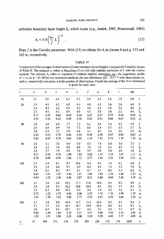
TABLE IV
Comparison ofthe averages of observations 6) and estimates (Z) on 6 heights z (m) and the 9 stability classes of Table II. The estimate 2, refers to Equations (7) or (14) with stability correction of L with the routine method. The estimate ?, refers to Equation (7) without stability correction, e.g., the logarithmic profile (L = co or $ = 0). Of the two estimation methods the rms differences {(X - Y)*}‘/* with observations (u, and 4, respectively) are given; n is the number of observations. Finally the average of the 10 m windspeed
is given for each class
z a b C d e f g h i All
10
20
2.1 3.9 5.4 6.3 5.2 3.9 3.3 2.6 1.9
2.4 4.5 2.4 4.3 2.5 4.5 0.17 0.50 0.21 0.50
40 2.4 4.8 2.6 4.8 2.8 5.1 0.25 0.52 0.46 0.63
80 2.6 5.1 2.8 5.2 3.1 5.7 0.51 0.76 0.78 0.99
120 2.7 5.4 2.9 5.4 3.4 6.1 0.63 1.01 0.94 1.22
160 2.7 5.6 3.0 5.6 3.5 6.3 0.72 1.22 1.01 1.38
200 2.7 5.8 3.1 5.7 3.6 6.5 0.84 1.49 1.05 1.55
n 41 196
6.2 6.8 6.1 6.2 6.9 6.2 6.2 6.9 6.0 0.62 0.49 0.36 0.62 0.49 0.36
6.9 7.7 7.2 6.9 7.9 7.3 7.7 7.9 6.8 0.70 0.64 0.54 0.74 0.64 0.69
7.6 8.9 9.0 7.6 9.0 8.8 7.9 9.0 7.6 0.76 1.00 1.02 0.99 1.00 1.71
8.1 9.7 10.6 8.0 9.7 9.9 8.5 9.7 8.1 1.07 1.46 1.61 1.26 1.46 2.87
8.4 10.3 11.7 8.3 10.2 10.8 8.8 10.2 8.5 1.33 1.86 2.06 1.62 1.86 3.77
8.8 10.9 12.7 8.5 10.7 16.7 9.1 10.7 8.7 1.64 2.21 2.51 1.86 2.21 4.60
171 134 276
4.8 4.2 3.6 2.9 4.8 4.2 3.4 2.6 4.5 3.8 3.0 2.2 0.27 0.27 0.29 0.44 0.43 0.51 0.64 0.67
6.1 5.6 5.0 4.2 6.0 5.4 4.7 3.5 5.1 4.3 3.4 2.6 0.49 0.58 0.67 0.94 1.10 1.42 1.74 1.76
8.3 7.8 6.8 5.6 7.6 7.2 6.3 4.5 5.7 4.8 3.8 2.9 1.20 1.17 1.19 1.67 2.77 3.16 3.24 2.98
9.4 9.3 7.8 6.1 8.9 8.5 7.4 5.2 6.7 5.1 4.1 3.3 1.84 1.60 1.54 1.88 4.21 4.40 4.09 3.48
11.0 10.0 8.1 6.3 10.0 9.5 8.2 5.7
6.4 5.4 4.2 3.2 2.22 1.78 1.76 ,1.98 5.15 4.97 4.33 3.64
11.6 10.4 8.3 6.5 10.9 10.4 8.8 6.1
6.6 5.5 4.4 I 3.3 2.41 2.04 2.05 2.11 5.69 5.29 4.45 3.77
4.0 j
4.8 j 4.8 X1 4.6 X2 0.40 0, 0.52 u2
5.9 j 5.7 x, 5.2 X, 0.63 u, 1.16 u2
7.3 j 7.0 x, 5.8 j2, 1.11 cr, 2.31 a,
8.4 j 7.8 x, 6.2 X, 1.52 u, 3.19 fJ2
8.9 j 8.5 z, 6.5 jz, 1.79 u, 3.70 u*
9.4 7 9.1 sz, 6.7 X2 2.06 u, 4.09 CT2
209 228 174 176 1605 n
240 A. A. M. HOLTSLAG
Well above the boundary layer, of course, the wind speed should approach the ‘free’ or geostrophic wind speed G. The latter, however, might be obscured by the presence of gravity waves or a low-level jet. In such cases, no simple estimate can be made anymore of the wind profile from surface data only. Perhaps an interpolation formula between surface-layer wind speed and geostrophic wind speed is more suitable for these stable conditions (e.g., Van Ulden and Holtslag, 1980). This subject, however, needs more future research and is beyond the scope of the present study.
7. Results with Near-surface Weather Observations
In this section, we apply the findings of the preceding sections for derivation of the wind profile from near-surface weather data only. First the Obukhov length scale is estimated with the routine method (see Appendix). After this, (7) is used with tiM given by (8a) for unstable conditions and $M given by (8~) for stable conditions with z I 0.5 L. For z > 0.5 L in stable conditions, we use (14). Further observed 10 m wind speed is used for U, in (7) or (14).
Table IV contains averages of both observed (L) and estimated (Ei) wind speed for the 6 Cabauw levels. Also therms difference 6, between observations and estimates with the above scheme is given. We have used the whole data set as described in Section 3. Again we distinguish classes of stability as given in Table II, from very unstable to very stable conditions. For comparison, we have given the results of the logarithmic profile without any stability correction as well. These are denoted by K and cr,. The logarithmic profile is obtained with (7) using L = cc or & = 0. This results in a constant ratio between U, and U,, for given surface roughness length z,.
From Table IV, it is seen that the agreement between estimates and observations varies with height and stability. For the near-neutral conditions of class d, the stability correction is small and therefore cr = pi = a,. For this class, CT amounts to 0 = 1 m s - ’ at the 80 m level, which is N 11% of the observed average (j). At 200 m 0 = 2.2 m s - ‘, which is 20% of J. For the unstable conditions b and c, about the same relative accuracy (oi/$ is found. For class a o1 = 0.5 m s- ’ at 80 m, which is -20% of JJ. When (8b) is used instead of (8a), we obtain comparable results with our calculations. This confirms our findings in Figure 2. Up to 40 m, the accuracy of the logarithmic profile might also be acceptable, but above this height, o, is typically 25% larger than CJ, for unstable conditions. This is also true for the bias (y-x).
The stable conditions of class e and f have about the same relative accuracy as was found for class d. For the very stable conditions of class h, cr = 1.2 m s - ’ or -25% of 7. Note that for the stable conditions c~i is.less than, typically, 50% of a,. This means that the stability correction of the scheme improves the agreement with observations markedly.
Over all stabilities r~i = 0.6 m s - ’ at 40 m (11% of y)), as can be seen from Table IV. In Figure 5 we have illustrated the good agreement at this level. In the figure, a distinction is made between stable conditions (triangles) and unstable conditions (squares) with a random selection of the data in Table IV. In Figure 6, the relatively good
DIABATIC WIND PROFILES 241
“40 obs (ms-‘1
20
15
10
5
0
15 20
” 40 est (ms-‘1
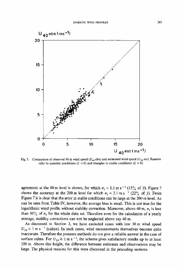
Fig. 5. Comparison of observed 40 m wind speed (U,, obs) and estimated wind speed (U,, est). Squares refer to unstable conditions (L < 0) and triangles to stable conditions (L > 0).
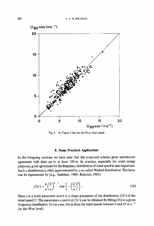
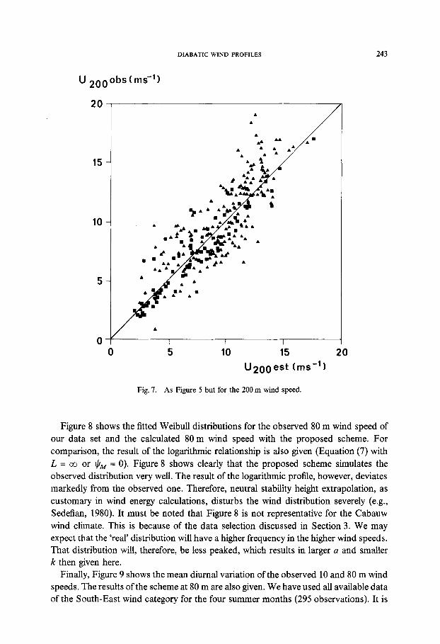
agreement at the 80 m level is shown, for which o1 = 1.1 m s - ’ (15 y0 of L). Figure 7 shows the accuracy at the 200 m level for which (ri = 2.1 m s - ’ (22% of J). From Figure 7 it is clear that the error in stable conditions can be large at the 200 m level. As can be seen from Table IV, however, the average bias is small. This is not true for the logarithmic wind profile without stability correction. Moreover, above 40 m, cri is less than 50% of o, for the whole data set. Therefore even for the calculation of a yearly average, stability corrections can not be neglected above say 40 m.
As discussed in Section 3, we have excluded cases with low 10 m wind speed U,, < 1 m s- ’ (calms). In such cases, wind measurements themselves become quite inaccurate. Therefore the presents methods do not give a reliable answer in the case of surface calms. For U,, 2 1 m s - ‘, the scheme gives satisfactory results up to at least 100 m. Above this height, the difference between estimates and observations may be large. The physical reasons for this were discussed in the preceding sections.
A. A. M. HOLTSLAG
0 5 10 15 20
u8OeSt (mS-'1
Fig. 6. As Figure 5 but for the 80 m wind speed.
8. Some Practical Applications
In the foregoing sections we have seen that the proposed scheme gives satisfactory agreement with data up to at least 100 m. In practice, especially for wind energy purposes, good agreement for the frequency distribution of wind speed is also important. Such a distribution is often approximated by a so-called Weibull distribution. The latter can be represented by (e.g., Sedefian, 1980; Rijkoort, 1983)
f(lJ)=t(:)j-‘exp{-(ty}. (16)
Here a is a scale parameter and k is a shape parameter of the distribution f(U) of the wind speed U. The parameters a and k off(U) can be obtained by fitting (16) to a given frequency distribution. In our case, this is done for wind speeds between 4 and 15 m s - ’ (at the 80 m level).
DIABATIC WIND PROFILES 243
“200 obs ( ms-‘1
5 10 15 20
U200est (ms-‘I
Fig. 7. As Figure 5 but for the 200 m wind speed.
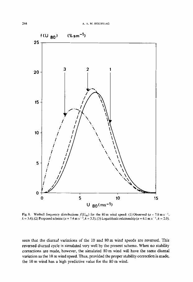
Figure 8 shows the fitted Weibull distributions for the observed 80 m wind speed of our data set and the calculated 80 m wind speed with the proposed scheme. For comparison, the result of the logarithmic relationship is also given (Equation (7) with L = co or I+& = 0). Figure 8 shows clearly that the proposed scheme simulates the observed distribution very well. The result of the logarithmic profile, however, deviates markedly from the observed one. Therefore, neutral stability height extrapolation, as customary in wind energy calculations, disturbs the wind distribution severely (e.g., Sedefian, 1980). It must be noted that Figure 8 is not representative for the Cabauw wind climate. This is because of the data selection discussed in Section 3. We may expect that the ‘real’ distribution will have a higher frequency in the higher wind speeds. That distribution will, therefore, be less peaked, which results in larger a and smaller k then given here.
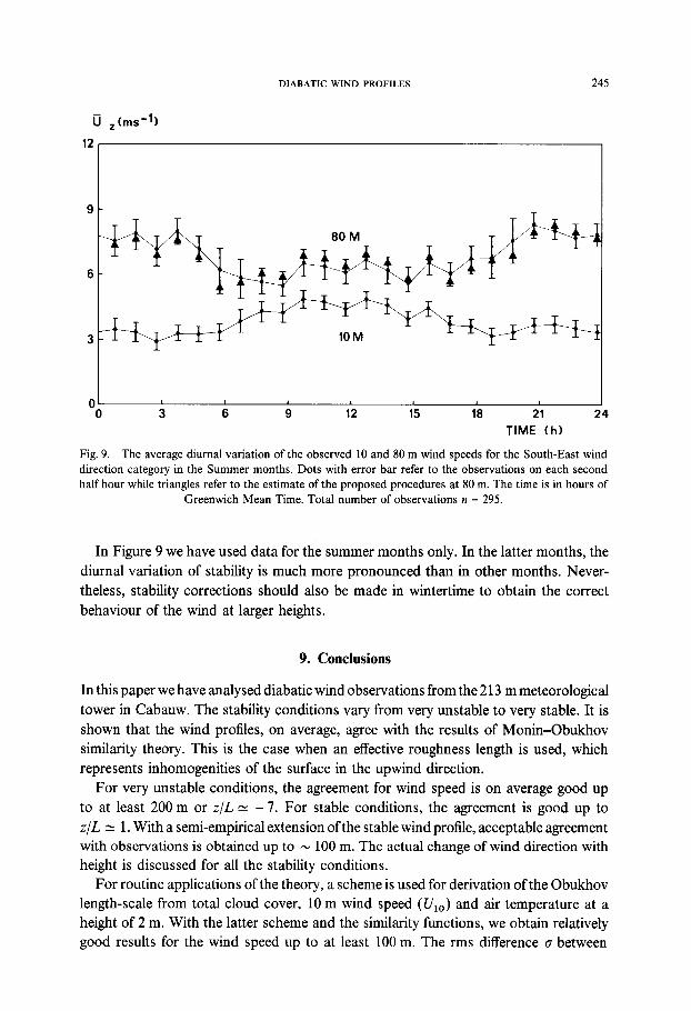
Finally, Figure 9 shows the mean diurnal variation of the observed 10 and 80 m wind speeds. The results of the scheme at 80 m are also given. We have used all available data of the South-East wind category for the four summer months (295 observations). It is
244 A. A. M. HOLTSLAG
25
20
15
10
5
0
f(lJ 80) (% sm")
0 5 10 15
U Bo(rns-1)
Fig. 8. Weibull frequency distributions f(Us,) for the 80 m wind speed: (1) Observed (a = 7.8 m s- ‘, k = 3.4); (2) Proposed scheme (a = 7.4 m s- I, k = 3.3); (3) Logarithmic relationship (a = 6.1 m s - ‘, k = 2.0).
seen that the diurnal variations of the 10 and 80 m wind speeds are reversed. This reversed diurnal cycle is simulated very well by the present scheme. When no stability corrections are made, however, the simulated 80 m wind will have the same diurnal variation as the 10 m wind speed. Thus, provided the proper stability correction is made, the 10 m wind has a high predictive value for the 80 m wind.
DIABATIC WIND PROFILES 245
01 0 3
I 6 9 12 15 18 21 24
TIME (h)
Fig. 9. The average diurnal variation of the observed 10 and 80 m wind speeds for the South-East wind direction category in the Summer months. Dots with error bar refer to the observations on each second half hour while triangles refer to the estimate of the proposed procedures at 80 m. The time is in hours of
Greenwich Mean Time. Total number of observations n = 295.
In Figure 9 we have used data for the summer months only. In the latter months, the diurnal variation of stability is much more pronounced than in other months. Never- theless, stability corrections should also be made in wintertime to obtain the correct behaviour of the wind at larger heights.
9. Conclusions
In this paper we have analysed diabatic wind observations from the 2 13 m meteorological tower in Cabauw. The stability conditions vary from very unstable to very stable. It is shown that the wind profiles, on average, agree with the results of Monin-Obukhov similarity theory. This is the case when an effective roughness length is used, which represents inhomogenities of the surface in the upwind direction.
For very unstable conditions, the agreement for wind speed is on average good up to at least 200 m or z/L N - 7. For stable conditions, the agreement is good up to z/L N 1. With a semi-empirical extension of the stable wind profile, acceptable agreement with observations is obtained up to N 100 m. The actual change of wind direction with height is discussed for all the stability conditions.
For routine applications of the theory, a scheme is used for derivation of the Obukhov length-scale from total cloud cover, 10 m wind speed (Vi,) and air temperature at a height of 2 m. With the latter scheme and the similarity functions, we obtain relatively good results for the wind speed up to at least 100 m. The rms difference rr between
246 A. A. M. HOLTSLAG
estimates and observations at 80 m is for all stabilities c N 1.1 m s- ‘, which is 15% of the observed average.
Above 100 m, the estimate of wind speed is still useful in unstable and moderately stable conditions. But in very stable conditions, the agreement is poorer. At 200 m for example, c varies between 0.8 m s - ’ for very unstable conditions to 2.1 m s - ’ for very stable conditions. Nevertheless, 0 is reduced by typically 50% in comparison with that of the logarithmic wind profile, in which stability correction is neglected. In surface calms (U,, < 1 m s - ‘), the present methods do not give a reliable answer.
As discussed in the paper, the proposed procedures can serve as an alternative for the empirical power law with exponents related to stability categories. The procedures simulate the reversed diurnal variation of the 80 m wind speed very well. Also the simulated frequency distribution of the 80 m wind speed agrees well with the observed one. Therefore, the present methods are suitable for applied meteorological studies up to at least 100 m in generally level terrain.
Acknowledgements
I am indebted to all the people at the Institute who worked on the preparation of the Cabauw data set. I would also like to thank A. C. M. Beljaars, F. T. M. Nieuwstadt, A. P. van Ulden, and J. Wieringa for stimulating discussions and useful comments on a draft of this paper.
Appendix: Derivation of the Obukhov Length Scale from Near-Surface Weather Data with Parameterized Sensible Heat Flux and Temperature Scale
For application of Equations (7) and (14), the Obukhov length scale L defined by (1) is needed. Section 4 discussed two methods for the derivation of L. Here a summary of the routine method is given, in which the sensible heat flux or the temperature scale is parameterized. For unstable conditions, we use the procedure developed by Holtslag and Van Ulden (1983). First, the incoming solar radiation K + is calculated from total cloud cover N and solar elevation $:
K + = (1041 sin $ - 69) (1 - 0.75N3.4). (AlI
A simple procedure for the calculation of $ for given time and location can be found in Holtslag and Van Ulden. Next, net radiation Q* is calculated from K + , N, the albedo r, air temperature T(K) and surface heating coefficient c3 by
Q*="-"K+ +c,T6-oT4+c2N 1 + c3
642)
We use I = 0.23, ci = 5.31 x lo-l3 W rnp2 Kp6, c = 5.67 x lo-* W m-’ Ke4, c2 = 60 W m-’ and c3 = 0.12. Values of r and c3 for other surface conditions are discussed by Holtslag and Van Ulden.
DIABATIC WIND PROFILES 241
Finally H is obtained from (De Bruin and Holtslag, 1982)
HJ-a+Yls 1 + rls
<Q* - G) - P, 643)
where
G=c,Q*.
643)
Here y/s is a universal thermodynamic function of air temperature (see Holtslag and Van Ulden). In (A3)-(A4) we use tl = 1, /I = 20 W m- 2, and cG = 0.1. The present values of the coefficients in (Al)-(A4) are shown to be suitable for typical climate and surface conditions in the Netherlands. For other sites, however, scarce turbulence measurements can be used to obtain adjusted values. In such cases the scheme can be applied to other conditions as well. A discussion on the variation of a, /I, cG, and cg with surface conditions is given in Holtslag and Van Ulden (1983). Of course, when measure- ments of K + , Q* or G are available, they can be incorporated into the scheme directly.
From (l), (2), and (9), L can be solved by iteration provided H is known by (Al)-(A4). We use the following procedure. The measured 10 m wind speed is used for U, and for T the air temperature at screen height (2 m) is used. For z,, the effective roughness length is taken. The computation starts with an estimate for u* by way of (9) where we take initially I& = 0 (L = co). In this way with (1) and (2), an estimate for L is obtained. With this estimate, (9) is used again to improve the estimate for u* and so on. It appears that not more than three iterations are needed in most cases to achieve an accuracy of 5% in successive values of L.
For stable conditions (L > 0) with solar elevation r#~ < 0, we parameterize L by using (Holtslag and Van Ulden, 1982)
8, = 0.09(1 - 0.5N2)) (-45)
where & is the turbulent temperature scale (K) related to L by (l), (2), and (12). Van Ulden and Holtslag (1983) showed that (A5) is a useful practical approximation to the rather complicated set of equations for the nighttime surface energy budget. Moreover, 6% of (A5) is in agreement with &. = 0.08 K obtained by Venkatram (1980) for mainly clear sky conditions in the Prairie Grass, Kansas and Minnesota data sets.
With (l), (2), (8c), (9), and (12), we can obtain a quadratic equation in L, whose solution can be written as
L = (L, - L,) + {L,(L, - 2L,)}“2 . (-46)
Here L, and L, are length scales given by
647)
248
and
A. A. M. HOLTSLAG
where 8, is given by (A5), a = 5, k = 0.41, g = 9.81 m ss2, z = 10 m, and T is air temperature (K). From (A5)-(A@, L can be calculated for given 10 m wind speed vi,,, total cloud cover N and surface roughness length z,,. Real solutions exist, however, for L, 2 2L, only. The lower limit for L = L, 1: 12.8 m for z, = 0.2 m and T = 288 K.
It appears that the model gives real solutions for L, if L 2 12.8 m. As discussed in Sections 4 and 6, lower values of L refer to the very stable case i, in which there is little or no turbulence. A simple practical solution for L < L, is obtained by using
( > 112
L= Lo2 ) 649)
which is continuous for L = L, and which results in L = 0 for U,, = 0. With (A9) and (14), we obtain a crude but simple extension of the wind profile in very stable conditions. As discussed in Section 7, the agreement with observations is still useful for practical applications.
Finally, we discuss the estimates of L in transition periods with L > 0 and $ > 0. In these periods the nighttime scheme is used as well, but here & is calculated from
a=s,{1-($], (All)
where 0~ is the value given by (A5). Here c$,, is the solar elevation for which H = 0. The latter can be obtained by putting H = 0 in (A3) and solving Q* with the aid of (A4). With this value of Q*, K + is calculated from (A2) and finally c#+, from (Al). It appears that, on average, c$” 1: 13 deg for N < 0.75 increasing to &, N 23 deg for N = 1 (Holtslag and Van Ulden, 1983).
References
Andre, J. C.: 1983, ‘On the Variability of the Nocturnal Boundary-Layer Depth’, J. Atmos. Sci. 40, 2309-2311.
Beljaars, A. C. M.: 1982, ‘The Derivation of Fluxes from Profiles in Perturbed Areas’, Boundary-Layer Meteorol. 24, 35-55.
Beljaars, A. C. M., Schotanus, P., and Nieuwstadt, F. T. M.: 1983, ‘Surface Layer Similarity under Non- uniform Fetch Conditions’, J. C. Appl. Meteorol. 22, 1800- 1810.
Berkowitz, R. and Prahm, L. P.: 1982, ‘Evaluation of the Profile Method for Estimation of Surface Fluxes of Momentum and Heat’, Atm. Env. 16, 2809-2819.
Cats, G. J.: 1980, ‘Analysis of Surface Wind and Its Gradient in a Mesoscale Wind Observations Network’, Monthly Weather Rev. 108, 1100-l 107.
Carson, D. J. and Richards, P. J. R.: 1978, ‘Modelling Surface Turbulent Fluxes in Stable Conditions’, Boundary-Layer Meteorol. 14, 67-8 1.
DIABATIC WIND PROFILES 249
Carl, D. M., Tarbell, T. C., and Panofsky, H. A.: 1973, ‘Profiles of Wind and Temperature from Towers over Homogeneous Terrain’, J. Atmos. Sci. 30, 788-794.
De Bruin, H. A. R. and Holtslag, A. A. M.: 1982, ‘A Simple Parameterization of the Surface Fluxes of Sensible and Latent Heat During Daytime Compared with the Penman-Monteith Concept’, J. Appl. Meteorol. 21, 1610-1621.
Driedonks, A. G. M., Van Dop, H., and Kohsiek, W.: 1978, ‘Meteorological Observations on the 213 Mast at Cabauw, in the Netherlands’, Fourth Symposium on Meteorol. Ohs. and Inst., April 10-14, 41-46. Published by Amer. Meteorol. Sot.
Dyer, A. J.: 1974, ‘A Review of Flux-Profile Relationships’, Boundary-Layer Meteorol. I, 363-372. Fiedler, F. and Panofsky, H. A.: 1972, ‘The Geostrophic Drag Coefficient and the Effective Roughness
Length’, Quart. J. Roy. Meteorol. Sot. 98, 213-220. Gill, G. C., Olson, L. E., Sela, J., and Suds, M.: 1967, ‘Accuracy of Wind Measurements on Towers or
Stacks’, Bull. Am. Meteorol. Sot. 48, 665-674. Golder, D.: 1972, ‘Relations Among Stability Parameters in the Surface Layer’, Boundary-Layer Meteorol.
3, 47-58. Hicks, B. B.: 1976, ‘Wind Profile Relatinships from the “Wangara” Experiment’, Quart. J. R. Meteorol. Sot.
102,535-551. Holtslag, A. A. M. and Van Ulden, A. P.: 1982, ‘Simple Estimates of Nighttime Surface Fluxes from Routine
Weather Data’, Scientific Report 82-4, Royal Netherlands Meteorological Institute, De Bilt, 15 pp. Holtslag, A. A. M. and Van Ulden, A. P.: 1983, ‘A Simple Scheme for Daytime Estimates of the Surface
Fluxes from Routine Weather Data’, J. C. Appl. Meteorol. 22, 517-529. Korrell, A., Panofsky, H. A., and Rossi, R. J.: 1982, ‘Wind Profiles at the Boulder Tower’, Boundary-Layer
Meteorol. 22, 295-312. Lumley, J. L. and Panofsky, H. A.: 1964, The Structure of Atmospheric Turbulence, Interscience, London,
239 pp. McBean, G. A. (ed.): 1979, The Planetary Boundary Layer, Technical note No. 165, WMO Geneva, 201 pp. Monin, A. S. and Yaglom, A. M.: 1971, Statistical Fluid Mechanics: Mechanics of Turbulence, Vol. I, 3th
printing, MIT Press, London. Nieuwstadt, F. T. M.: 1978, ‘The Computation of the Friction Velocity u* and the Temperature Scale T*
from Temperature and Wind Velocity Profiles by Least-Square Methods’, Boundary-Layer Meteorol. 14, 235-246.
Nieuwstadt, F. T. M.: 1984, ‘A Model for the Stationary, Stable Boundary Layer’, Proc. Conference on Models of Turbulence and Dtfision in Stable Stratt$ed Regions of the Natural Environment, Cambridge. March 1983.
Paulson, C. A.: 1970, ‘The Mathematical Representation of Wind Speed and Temperature Profiles in the Unstable Atmospheric Surface Layer’, J. Appl. Meteorol. 9, 856-861.
Rijkoort, P. J.: 1983, ‘A Compound Weibull Model for the Description of Surface Wind Velocity Distribu- tions’, Scienti$c Report WR 83-13, Royal Netherlands Meteorological Institute, De Bilt, 35 pp.
Schultz, P.: 1979, ‘Estimation of Surface Stress from Wind’, Boundary-Layer Meteorol. 17, 265-267. Sedefian, L.: 1980, ‘On Vertical Extrapolation of Mean Wind Power Density’, J. Appl. Meteorol. 19,488-493. SethuRaman, S. and Brown, R. M.: 1976, ‘Validity of the Log-Linear Profile Relationship over a Rough
Terrain During Stable Conditions’, Boundary-Layer Meteorol. 10, 489-501. Tennekes, H.: 1982, ‘Similarity Relations, Scaling Laws and Spectral Dynamics’, in F. T. M. Nieuwstadt and
H. van Dop (eds.), Atmospheric Turbulence and Air Pollution Modelling, D. Reidel Publ. Co., Dordrecht, Holland, pp. 37-68.
Van Ulden, A. P. and Holtslag, A. A. M.: 1980, ‘The Wind at Heights Between 10 and 200 m in comparison with the Geostrophic Wind, Proc. Seminar on Radioactive Releases, Rise, 22-25 April, 1980, Commission E.C., Luxembourg, Vol. I, 83-92.
Van Ulden, A. P. and Holtslag, A. A. M.: 1983, The Stability of the Atmospheric Surface Layer During Nighttime’, Sixth Symp. on Turbulence and Dtfision, March 22-25, pp. 257-260. Published by Amer. Meteorol. Sot.
Venkatram, A.: 1980, ‘Estimating the Monin-Obukhov Length in the Stable Boundary Layer for Dispersion Calculations’, Boundary-Layer Meteorol. 19, 481-485.
Webb, E. K.: 1970, ‘Profile Relationships: The Log-Linear Range and Extension to Strong Stability’, Quart. J. Roy. Meteorol. Sot. 96, 67-90.
Wessels, H. R. A.: 1983, ‘Distortion of the Wind Field by the Cabauw Meteorological Tower’, Scientific Report 83-15, Royal Netherlands Meteorological Institute, De Bilt, 34 pp.
250 A. A. M. HOLTSLAG
Wieringa, J.: 1976, ‘An Objective Exposure Correction Method for Average Wind Speeds Measured at a Sheltered Location’, Quart. J. Roy. Meteorol. Sot. 102, 241-253.
Wieringa, J.: 1980, ‘Representativeness of Wind Observations at Airports’, Bull. Amer. Meteorol. Sot. 61, 962-971.
Wieringa, J.: 1981, ‘Estimation of Mesoscale and Local-Scale Roughness for Atmospheric Transport Modeling’, Air Pollution Modeling and its Application, Plenum, New York, pp. 279-295.
Wieringa, J.: 1983, ‘Description Requirements for Assessment of Non-Ideal Wind Stations - for Example Aachen. J. Wind. Eng. Industr. Aerod. 11, 121-131.
Yaglom, A. M.: 1977, ‘Comments on Wind and Temperature Flux-Profile Relationships’, Boundary-Layer Meteorol. 11. 89- 102.