Published as a conference paper at ICLR 2018

A ADVERSARIAL DOMAIN ADAPTATION (ADA)

ADA aims to transfer prediction knowledge learned from a source domain with labeled data to atarget domain without labels, by learning domain-invariant features. Let Dφ(x) = qφ(y|x) be thedomain discriminator. The conventional formulation of ADA is as following:

maxφ Lφ = Ex=Gθ(z),z∼p(z|y=1) [logDφ(x)] + Ex=Gθ(z),z∼p(z|y=0) [log(1−Dφ(x))] ,

maxθ Lθ = Ex=Gθ(z),z∼p(z|y=1) [log(1−Dφ(x))] + Ex=Gθ(z),z∼p(z|y=0) [logDφ(x)] .(18)

Further add the supervision objective of predicting label t(z) of data z in the source domain, with aclassifier fω(t|x) parameterized with π:

maxω,θ Lω,θ = Ez∼p(z|y=1) [log fω(t(z)|Gθ(z))] . (19)

We then obtain the conventional formulation of adversarial domain adaptation used or similarin (Ganin et al., 2016; Purushotham et al., 2017).

B PROOF OF LEMMA 1

Proof.Epθ(x|y)p(y) [log q

r(y|x)] =− Ep(y) [KL (pθ(x|y)‖qr(x|y))− KL(pθ(x|y)‖pθ0(x))] ,

(20)

whereEp(y) [KL(pθ(x|y)‖pθ0(x))]

= p(y = 0) · KL(pθ(x|y = 0)‖pθ0(x|y = 0) + pθ0(x|y = 1)

2

)+ p(y = 1) · KL

(pθ(x|y = 1)‖pθ0(x|y = 0) + pθ0(x|y = 1)

2

).

(21)

Note that pθ(x|y = 0) = pgθ (x), and pθ(x|y = 1) = pdata(x). Let pMθ=

pgθ+pdata2 . Eq.(21) can

be simplified as:

Ep(y) [KL(pθ(x|y)‖pθ0(x))] =1

2KL(pgθ‖pMθ0

)+

1

2KL(pdata‖pMθ0

). (22)

On the other hand,

JSD(pgθ‖pdata) =1

2Epgθ

[log

pgθpMθ

]+

1

2Epdata

[log

pdatapMθ

]=

1

2Epgθ

[log

pgθpMθ0

]+

1

2Epgθ

[log

pMθ0pMθ

]

+1

2Epdata

[log

pdatapMθ0

]+

1

2Epdata

[log

pMθ0pMθ

]

=1

2Epgθ

[log

pgθpMθ0

]+

1

2Epdata

[log

pdatapMθ0

]+ EpMθ

[log

pMθ0pMθ

]=

1

2KL(pgθ‖pMθ0

)+

1

2KL(pdata‖pMθ0

)− KL

(pMθ‖pMθ0

).

(23)

Note that∇θKL

(pMθ‖pMθ0

)|θ=θ0 = 0. (24)

Taking derivatives of Eq.(22) w.r.t θ at θ0 we get∇θEp(y) [KL(pθ(x|y)‖pθ0(x))] |θ=θ0

= ∇θ(1

2KL(pgθ‖pMθ0

)|θ=θ0 +

1

2KL(pdata‖pMθ0

))|θ=θ0

= ∇θJSD(pgθ‖pdata) |θ=θ0 .

(25)

Taking derivatives of the both sides of Eq.(20) at w.r.t θ at θ0 and plugging the last equation ofEq.(25), we obtain the desired results.

14

Published as a conference paper at ICLR 2018

Note on Unification of GANs/VAEs/ADA/...

Zhiting Huzhitinghu@gmail.com

zsrc

ztgt

xsrc

xtgt

y

z

xreal

xfake

x

zgen

xgen

xdata

G✓

D�

p✓(x|y)

q�(y|x)/qr�(y|x)

q(r)� (y|x)

q⌘(z|x, y)

qr⇤(y|x)

q(r)⇤ (y|x)

p✓(x|z, y)

p✓(x|z, y)

q(r)� (y|z)

q⌘(z|y)

Note on Unification of GANs/VAEs/ADA/...

Zhiting Huzhitinghu@gmail.com

zsrc

ztgt

xsrc

xtgt

y

z

xreal

xfake

x

zgen

xgen

xdata

G✓

D�

p✓(x|y)

q�(y|x)/qr�(y|x)

q(r)� (y|x)

q⌘(z|x, y)

qr⇤(y|x)

q(r)⇤ (y|x)

p✓(x|z, y)

p✓(x|z, y)

q(r)� (y|z)

q⌘(z|y)

Note on Unification of GANs/VAEs/ADA/...

Zhiting Huzhitinghu@gmail.com

zsrc

ztgt

xsrc

xtgt

y

z

xreal

xfake

x

zgen

xgen

xdata

G✓

D�

p✓(x|y)

q�(y|x)/qr�(y|x)

q(r)� (y|x)

q⌘(z|x, y)

qr⇤(y|x)

p✓(x|z, y)

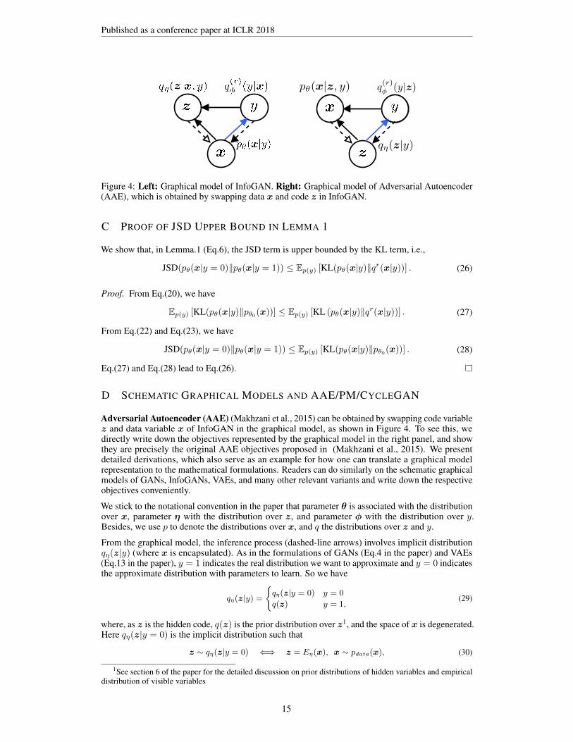
Figure 4: Left: Graphical model of InfoGAN. Right: Graphical model of Adversarial Autoencoder(AAE), which is obtained by swapping data x and code z in InfoGAN.

C PROOF OF JSD UPPER BOUND IN LEMMA 1

We show that, in Lemma.1 (Eq.6), the JSD term is upper bounded by the KL term, i.e.,

JSD(pθ(x|y = 0)‖pθ(x|y = 1)) ≤ Ep(y) [KL(pθ(x|y)‖qr(x|y))] . (26)

Proof. From Eq.(20), we have

Ep(y) [KL(pθ(x|y)‖pθ0(x))] ≤ Ep(y) [KL (pθ(x|y)‖qr(x|y))] . (27)

From Eq.(22) and Eq.(23), we have

JSD(pθ(x|y = 0)‖pθ(x|y = 1)) ≤ Ep(y) [KL(pθ(x|y)‖pθ0(x))] . (28)

Eq.(27) and Eq.(28) lead to Eq.(26).

D SCHEMATIC GRAPHICAL MODELS AND AAE/PM/CYCLEGAN

Adversarial Autoencoder (AAE) (Makhzani et al., 2015) can be obtained by swapping code variablez and data variable x of InfoGAN in the graphical model, as shown in Figure 4. To see this, wedirectly write down the objectives represented by the graphical model in the right panel, and showthey are precisely the original AAE objectives proposed in (Makhzani et al., 2015). We presentdetailed derivations, which also serve as an example for how one can translate a graphical modelrepresentation to the mathematical formulations. Readers can do similarly on the schematic graphicalmodels of GANs, InfoGANs, VAEs, and many other relevant variants and write down the respectiveobjectives conveniently.

We stick to the notational convention in the paper that parameter θ is associated with the distributionover x, parameter η with the distribution over z, and parameter φ with the distribution over y.Besides, we use p to denote the distributions over x, and q the distributions over z and y.

From the graphical model, the inference process (dashed-line arrows) involves implicit distributionqη(z|y) (where x is encapsulated). As in the formulations of GANs (Eq.4 in the paper) and VAEs(Eq.13 in the paper), y = 1 indicates the real distribution we want to approximate and y = 0 indicatesthe approximate distribution with parameters to learn. So we have

qη(z|y) =

{qη(z|y = 0) y = 0

q(z) y = 1,(29)

where, as z is the hidden code, q(z) is the prior distribution over z1, and the space of x is degenerated.Here qη(z|y = 0) is the implicit distribution such that

z ∼ qη(z|y = 0) ⇐⇒ z = Eη(x), x ∼ pdata(x), (30)

1See section 6 of the paper for the detailed discussion on prior distributions of hidden variables and empiricaldistribution of visible variables

15

Published as a conference paper at ICLR 2018

where Eη(x) is a deterministic transformation parameterized with η that maps data x to code z.Note that as x is a visible variable, the pre-fixed distribution of x is the empirical data distribution.

On the other hand, the generative process (solid-line arrows) involves pθ(x|z, y)q(r)φ (y|z) (here q(r)

means we will swap between qr and q). As the space of x is degenerated given y = 1, thus pθ(x|z, y)is fixed without parameters to learn, and θ is only associated to y = 0.

With the above components, we maximize the log likelihood of the generative distributionslog pθ(x|z, y)q(r)φ (y|z) conditioning on the variable z inferred by qη(z|y). Adding the prior distri-butions, the objectives are then written as

maxφ Lφ = Eqη(z|y)p(y) [log pθ(x|z, y)qφ(y|z)]maxθ,η Lθ,η = Eqη(z|y)p(y)

[log pθ(x|z, y)qrφ(y|z)

].

(31)

Again, the only difference between the objectives of φ and {θ,η} is swapping between qφ(y|z) andits reverse qrφ(y|z).To make it clearer that Eq.(31) is indeed the original AAE proposed in (Makhzani et al., 2015), wetransform Lφ as

maxφ Lφ = Eqη(z|y)p(y) [log qφ(y|z)]

=1

2Eqη(z|y=0) [log qφ(y = 0|z)] + 1

2Eqη(z|y=1) [log qφ(y = 1|z)]

=1

2Ez=Eη(x),x∼pdata(x) [log qφ(y = 0|z)] + 1

2Ez∼q(z) [log qφ(y = 1|z)] .

(32)

That is, the discriminator with parameters φ is trained to maximize the accuracy of distinguishing thehidden code either sampled from the true prior p(z) or inferred from observed data example x. Theobjective Lθ,η optimizes θ and η to minimize the reconstruction loss of observed data x and at thesame time to generate code z that fools the discriminator. We thus get the conventional view of theAAE model.

Predictability Minimization (PM) (Schmidhuber, 1992) is the early form of adversarial approachwhich aims at learning code z from data such that each unit of the code is hard to predict by theaccompanying code predictor based on remaining code units. AAE closely resembles PM by seeingthe discriminator as a special form of the code predictors.

CycleGAN (Zhu et al., 2017) is the model that learns to translate examples of one domain (e.g.,images of horse) to another domain (e.g., images of zebra) and vice versa based on unpaired data.Let x and z be the variables of the two domains, then the objectives of AAE (Eq.31) is preciselythe objectives that train the model to translate x into z. The reversed translation is trained with theobjectives of InfoGAN (Eq.9 in the paper), the symmetric counterpart of AAE.

E PROOF OF LEMME 2

Proof. For the reconstruction term:

Epθ0 (x)

[Eqη(z|x,y)qr∗(y|x) [log pθ(x|z, y)]

]=

1

2Epθ0 (x|y=1)

[Eqη(z|x,y=0),y=0∼qr∗(y|x) [log pθ(x|z, y = 0)]

]+

1

2Epθ0 (x|y=0)

[Eqη(z|x,y=1),y=1∼qr∗(y|x) [log pθ(x|z, y = 1)]

]=

1

2Epdata(x)

[Eq̃η(z|x) [log p̃θ(x|z)]

]+ const,

(33)

where y = 0 ∼ qr∗(y|x) means qr∗(y|x) predicts y = 0 with probability 1. Note that both qη(z|x, y =1) and pθ(x|z, y = 1) are constant distributions without free parameters to learn; qη(z|x, y = 0) =q̃η(z|x), and pθ(x|z, y = 0) = p̃θ(x|z).

16

Published as a conference paper at ICLR 2018

For the KL prior regularization term:Epθ0 (x) [KL(qη(z|x, y)qr∗(y|x)‖p(z|y)p(y))]

= Epθ0 (x)

[∫qr∗(y|x)KL (qη(z|x, y)‖p(z|y)) dy + KL (qr∗(y|x)‖p(y))

]=

1

2Epθ0 (x|y=1) [KL (qη(z|x, y = 0)‖p(z|y = 0)) + const] +

1

2Epθ0 (x|y=1) [const]

=1

2Epdata(x) [KL(q̃η(z|x)‖p̃(z))] .

(34)

Combining Eq.(33) and Eq.(34) we recover the conventional VAE objective in Eq.(7) in the paper.

F VAE/GAN JOINT MODELS FOR MODE MISSING/COVERING

Previous works have explored combination of VAEs and GANs. This can be naturally motivated bythe asymmetric behaviors of the KL divergences that the two algorithms aim to optimize respectively.Specifically, the VAE/GAN joint models (Larsen et al., 2015; Pu et al., 2017) that improve thesharpness of VAE generated images can be alternatively motivated by remedying the mode coveringbehavior of the KLD in VAEs. That is, the KLD tends to drive the generative model to cover allmodes of the data distribution as well as regions with small values of pdata, resulting in blurred,implausible samples. Incorporation of GAN objectives alleviates the issue as the inverted KL enforcesthe generator to focus on meaningful data modes. From the other perspective, augmenting GANswith VAE objectives helps addressing the mode missing problem, which justifies the intuition of (Cheet al., 2017a).

G IMPORTANCE WEIGHTED GANS (IWGAN)

From Eq.(6) in the paper, we can view GANs as maximizing a lower bound of the “marginallog-likelihood” on y:

log q(y) = log

∫pθ(x|y)

qr(y|x)pθ0(x)pθ(x|y)

dx

≥∫

pθ(x|y) logqr(y|x)pθ0(x)

pθ(x|y)dx

= −KL(pθ(x|y)‖qr(x|y)) + const.

(35)

We can apply the same importance weighting method as in IWAE (Burda et al., 2015) to derive atighter bound.

log q(y) = logE

[1

k

k∑i=1

qr(y|xi)pθ0(xi)pθ(xi|y)

]

≥ E

[log

1

k

k∑i=1

qr(y|xi)pθ0(xi)pθ(xi|y)

]

= E

[log

1

k

k∑i=1

wi

]:= Lk(y)

(36)

where we have denoted wi =qr(y|xi)pθ0 (xi)

pθ(xi|y) , which is the unnormalized importance weight. Werecover the lower bound of Eq.(35) when setting k = 1.

To maximize the importance weighted lower bound Lk(y), we take the derivative w.r.t θ and applythe reparameterization trick on samples x:

∇θLk(y) = ∇θEx1,...,xk

[log

1

k

k∑i=1

wi

]= Ez1,...,zk

[∇θ log

1

k

k∑i=1

w(y,x(zi,θ))

]

= Ez1,...,zk

[k∑i=1

w̃i∇θ logw(y,x(zi,θ))

],

(37)

17

Published as a conference paper at ICLR 2018

where w̃i = wi/∑ki=1 wi are the normalized importance weights. We expand the weight at θ = θ0

wi|θ=θ0 =qr(y|xi)pθ0(xi)

pθ(xi|y)= qr(y|xi)

12pθ0(xi|y = 0) + 1

2pθ0(xi|y = 1)

pθ0(xi|y)|θ=θ0 . (38)

The ratio of pθ0(xi|y = 0) and pθ0(xi|y = 1) is intractable. Using the Bayes’ rule and approximatingwith the discriminator distribution, we have

p(x|y = 0)

p(x|y = 1)=

p(y = 0|x)p(y = 1)

p(y = 1|x)p(y = 0)≈ q(y = 0|x)

q(y = 1|x) . (39)

Plug Eq.(39) into the above we have

wi|θ=θ0 ≈qr(y|xi)q(y|xi)

. (40)

In Eq.(37), the derivative ∇θ logwi is

∇θ logw(y,x(zi,θ)) = ∇θ log qr(y|x(zi,θ)) +∇θ logpθ0(xi)

pθ(xi|y). (41)

The second term in the RHS of the equation is intractable as it involves evaluating the likelihood ofimplicit distributions. However, if we take k = 1, it can be shown that

− Ep(y)p(z|y)[∇θ log

pθ0(x(z,θ))

pθ(x(z,θ)|y)|θ=θ0

]= −∇θ

1

2Epθ(x|y=0)

[pθ0(x)

pθ(x|y = 0)

]+

1

2Epθ(x|y=1)

[pθ0(x)

pθ(x|y = 1)

]|θ=θ0

= ∇θJSD(pgθ (x)‖pdata(x))|θ=θ0 ,

(42)

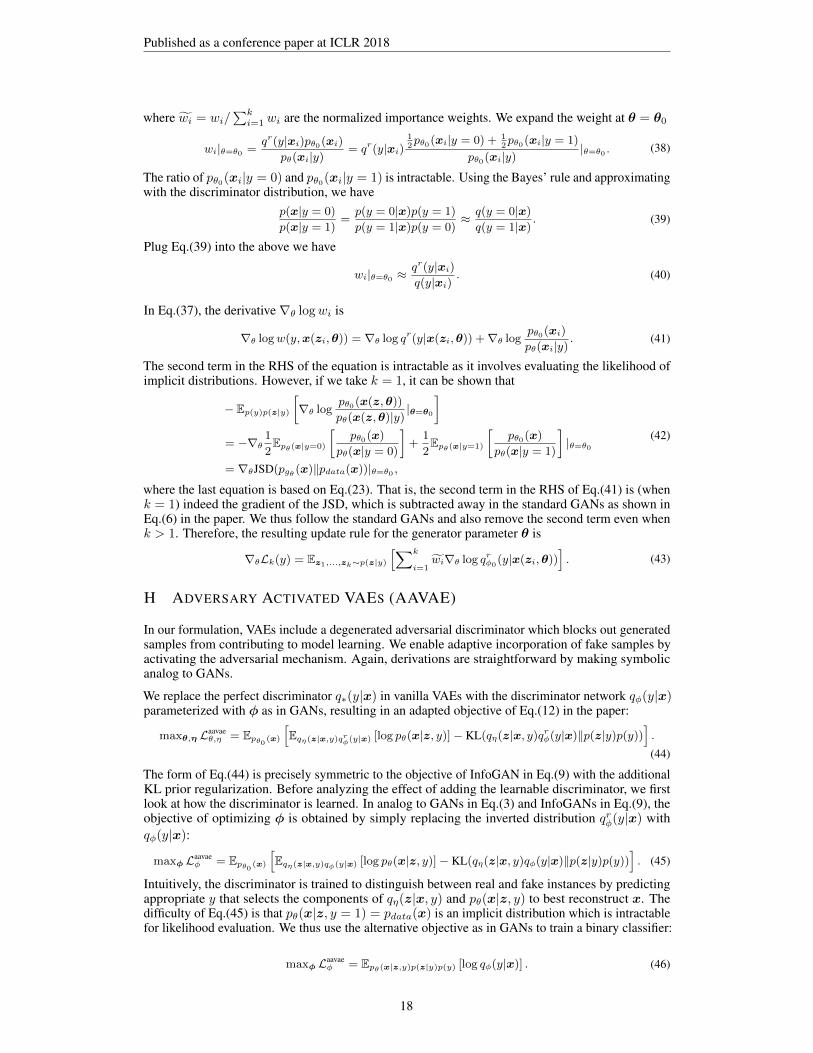
where the last equation is based on Eq.(23). That is, the second term in the RHS of Eq.(41) is (whenk = 1) indeed the gradient of the JSD, which is subtracted away in the standard GANs as shown inEq.(6) in the paper. We thus follow the standard GANs and also remove the second term even whenk > 1. Therefore, the resulting update rule for the generator parameter θ is

∇θLk(y) = Ez1,...,zk∼p(z|y)[∑k

i=1w̃i∇θ log qrφ0

(y|x(zi,θ))]. (43)

H ADVERSARY ACTIVATED VAES (AAVAE)

In our formulation, VAEs include a degenerated adversarial discriminator which blocks out generatedsamples from contributing to model learning. We enable adaptive incorporation of fake samples byactivating the adversarial mechanism. Again, derivations are straightforward by making symbolicanalog to GANs.

We replace the perfect discriminator q∗(y|x) in vanilla VAEs with the discriminator network qφ(y|x)parameterized with φ as in GANs, resulting in an adapted objective of Eq.(12) in the paper:

maxθ,η Laavaeθ,η = Epθ0 (x)

[Eqη(z|x,y)qrφ(y|x) [log pθ(x|z, y)]− KL(qη(z|x, y)qrφ(y|x)‖p(z|y)p(y))

].

(44)

The form of Eq.(44) is precisely symmetric to the objective of InfoGAN in Eq.(9) with the additionalKL prior regularization. Before analyzing the effect of adding the learnable discriminator, we firstlook at how the discriminator is learned. In analog to GANs in Eq.(3) and InfoGANs in Eq.(9), theobjective of optimizing φ is obtained by simply replacing the inverted distribution qrφ(y|x) withqφ(y|x):maxφ Laavae

φ = Epθ0 (x)

[Eqη(z|x,y)qφ(y|x) [log pθ(x|z, y)]− KL(qη(z|x, y)qφ(y|x)‖p(z|y)p(y))

]. (45)

Intuitively, the discriminator is trained to distinguish between real and fake instances by predictingappropriate y that selects the components of qη(z|x, y) and pθ(x|z, y) to best reconstruct x. Thedifficulty of Eq.(45) is that pθ(x|z, y = 1) = pdata(x) is an implicit distribution which is intractablefor likelihood evaluation. We thus use the alternative objective as in GANs to train a binary classifier:

maxφ Laavaeφ = Epθ(x|z,y)p(z|y)p(y) [log qφ(y|x)] . (46)

18

Published as a conference paper at ICLR 2018

I EXPERIMENTS

I.1 IMPORTANCE WEIGHTED GANS

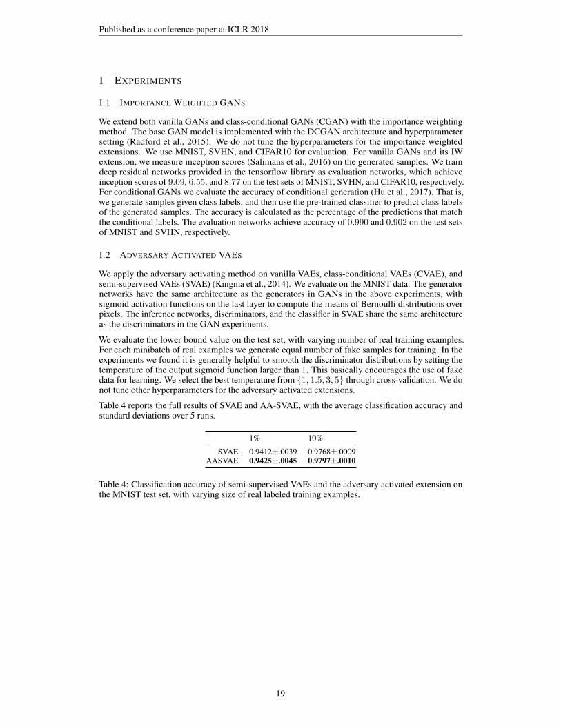
We extend both vanilla GANs and class-conditional GANs (CGAN) with the importance weightingmethod. The base GAN model is implemented with the DCGAN architecture and hyperparametersetting (Radford et al., 2015). We do not tune the hyperparameters for the importance weightedextensions. We use MNIST, SVHN, and CIFAR10 for evaluation. For vanilla GANs and its IWextension, we measure inception scores (Salimans et al., 2016) on the generated samples. We traindeep residual networks provided in the tensorflow library as evaluation networks, which achieveinception scores of 9.09, 6.55, and 8.77 on the test sets of MNIST, SVHN, and CIFAR10, respectively.For conditional GANs we evaluate the accuracy of conditional generation (Hu et al., 2017). That is,we generate samples given class labels, and then use the pre-trained classifier to predict class labelsof the generated samples. The accuracy is calculated as the percentage of the predictions that matchthe conditional labels. The evaluation networks achieve accuracy of 0.990 and 0.902 on the test setsof MNIST and SVHN, respectively.

I.2 ADVERSARY ACTIVATED VAES

We apply the adversary activating method on vanilla VAEs, class-conditional VAEs (CVAE), andsemi-supervised VAEs (SVAE) (Kingma et al., 2014). We evaluate on the MNIST data. The generatornetworks have the same architecture as the generators in GANs in the above experiments, withsigmoid activation functions on the last layer to compute the means of Bernoulli distributions overpixels. The inference networks, discriminators, and the classifier in SVAE share the same architectureas the discriminators in the GAN experiments.

We evaluate the lower bound value on the test set, with varying number of real training examples.For each minibatch of real examples we generate equal number of fake samples for training. In theexperiments we found it is generally helpful to smooth the discriminator distributions by setting thetemperature of the output sigmoid function larger than 1. This basically encourages the use of fakedata for learning. We select the best temperature from {1, 1.5, 3, 5} through cross-validation. We donot tune other hyperparameters for the adversary activated extensions.

Table 4 reports the full results of SVAE and AA-SVAE, with the average classification accuracy andstandard deviations over 5 runs.

1% 10%

SVAE 0.9412±.0039 0.9768±.0009AASVAE 0.9425±.0045 0.9797±.0010

Table 4: Classification accuracy of semi-supervised VAEs and the adversary activated extension onthe MNIST test set, with varying size of real labeled training examples.

19