A Bootstrap Lasso + Partial Ridge Method to Construct Con ... · lute coe cients from the largest to the smallest, ... 1.Our proposed Bootstrap LPR method relaxes the beta-min condition

A Bootstrap Lasso + Partial Ridge Methodto Construct Confidence Intervals for

Parameters in High-dimensional SparseLinear Models

Hanzhong Liu1, Xin Xu2, and Jingyi Jessica Li3,4,5

1Center for Statistical Science, Department of Industrial Engineering, Tsinghua University

2Department of Statistics, Yale University3Department of Statistics, University of California, Los Angeles, CA

4Department of Human Genetics, University of California, Los Angeles, CA5To whom correspondence should be addressed. Email: [email protected]

June 8, 2017

AbstractFor high-dimensional sparse linear models, how to construct confidence intervals for coef-ficients remains a difficult question. The main reason is the complicated limiting distri-butions of common estimators such as the Lasso. Several confidence interval constructionmethods have been developed, and Bootstrap Lasso+OLS is notable for its simple tech-nicality, good interpretability, and comparable performance with other more complicatedmethods. However, Bootstrap Lasso+OLS depends on the beta-min assumption, a theo-retic criterion that is often violated in practice. In this paper, we introduce a new methodcalled Bootstrap Lasso+Partial Ridge (LPR) to relax this assumption. LPR is a two-stageestimator: first using Lasso to select features and subsequently using Partial Ridge to re-fit the coefficients. Simulation results show that Bootstrap LPR outperforms BootstrapLasso+OLS when there exist small but non-zero coefficients, a common situation violat-ing the beta-min assumption. For such coefficients, compared to Bootstrap Lasso+OLS,confidence intervals constructed by Bootstrap LPR have on average 50% larger coverageprobabilities. Bootstrap LPR also has on average 35% shorter confidence interval lengthsthan the de-sparsified Lasso methods, regardless of whether linear models are misspeci-fied. Additionally, we provide theoretical guarantees of Bootstrap LPR under appropriateconditions and implement it in the R package “HDCI.”

KeywordsBootstrap, Lasso+Partial Ridge (LPR), confidence interval, model selection consistency,high-dimensional inference

1

arX

iv:1

706.

0215

0v1

[st

at.M

E]

7 J

un 2

017

1. Introduction

There has been rapid growth in the production and needs to analyze high dimensionaldata in a variety of fields including information technology, astronomy, neuroscience andbioinformatics, to name just a few. Data are high dimensional if the number of pre-dictors p is comparable to, or much larger than, the sample size n. Over the past twodecades, statistical and machine learning theory, methodology, and algorithms have beendeveloped to tackle high-dimensional data problems under certain sparsity constraints,e.g., the number of nonzero linear model coefficients s is much smaller than the samplesize n. Regularization is required to perform sparse estimation under this regime. Forexample, the Lasso [25] uses l1 regularization to perform model selection and param-eter estimation (to identify non-zero coefficients and estimate them as point estimateswithout confidence intervals) simultaneously in high dimensional sparse linear regres-sion. Previous work has focused on the recovery of a sparse parameter vector (denotedby β0 ∈ Rp) based on common criteria such as: (i) model selection consistency (theprobability that the procedure correctly identifies the support set of the β0 convergesto 1 as n → ∞); (ii) lq estimation error ||β − β0||q, where β is an estimate of β0 and q

typically equals 1 or 2; (iii) prediction error ||Xβ−Xβ0||2 with X as the design matrix.The book [5] and the review paper [10] give a thorough summary of the recent advancesin high dimensional statistics.

An important question at the frontier of high-dimensional statistical research is howto perform statistical inference, i.e., constructing confidence intervals and hypothesistests, for individual coefficients in linear models. Inference is crucial when the purposeof statistical modeling is to understand scientific principles beyond prediction. However,inference is difficult for high-dimensional model parameters, because the limiting dis-tribution of common estimators, for example the Lasso estimator, is complicated andhard to compute in high-dimensions. Facing this challenge, here we develop a novel andpractical inference procedure called Bootstrap Lasso+Partial Ridge, which is based onthree canonical methods: the Bootstrap, the Lasso and the Ridge. Before presentingour method, we first briefly review the existing high-dimensional inference methods inthe next two paragraphs.

There is a growing statistical literature that tackles high-dimensional inference prob-lems. Existing methods belong to several categories, including the sample splittingbased methods, the Bootstrap based methods, the de-sparsified Lasso methods, thepost-selection inference methods, and the knockoff filter. In particular, Wasserman andRoeder (2009) proposed a sample splitting method [28], which splits n data points intotwo halves, with the first half to be used for model selection (say by the Lasso) and thesecond half for constructing confidence intervals or p-values for the parameters in theselected model. For a fixed dimension p, Minnier et al. (2009) developed a perturbationresampling based method to approximate the distribution of penalized regression esti-mates under a general class of loss functions [23]. Chatterjee and Lahiri (2011) proposeda modified residual Bootstrap Lasso method [7], which is consistent in estimating thelimiting distribution of a modified Lasso estimator. For the scenarios with p going toinfinity at a polynomial rate of n, Chatterjee and Lahiri (2012) showed that a residual

2

Bootstrap adaptive Lasso estimator can consistently estimate the limiting distributionof the adaptive Lasso estimator under several intricate conditions [8], two of which aresimilar to the irrepresentible condition and the beta-min condition1 that together guar-antee the model selection consistency of the Lasso. Liu and Yu (2013) proposed anotherresidual Bootstrap method based on a two-stage estimator Lasso+OLS2 and showedconsistency under the irrepresentible condition, the beta-min condition and other regu-larity conditions [20]. A main issue with these methods is that they all require the ratherrestrictive beta-min condition, which should be better relaxed in high-dimensional infer-ence if possible.

Besides the above sample splitting or Bootstrap based methods, the de-sparsifiedLasso, which was first proposed by [29] and later investigated by [14, 26], is anothertype of methods. They aim to remove the biases of the Lasso estimates and producean asymptotically normal estimate for each individual parameter. Specifically, for thetwo typical de-sparsified Lasso methods developed by Zhang and Zhang (2011) [29] andJavanmard and Montanari (2013) [14], we will refer to them as LDPE (Low DimensionalProjection Estimator) and JM (“Javanmard and Montanari” in respect of the authors’names) in short in the following text. These methods do not rely on the beta-min con-dition but on the other hand require estimating the precision matrix of predictors usingthe graphical Lasso [26, 29] or another convex optimization procedure [14]. There arethree main issues with these methods. First, these methods require s log p/

√n → 0 as

n → ∞ to remove the asymptotic bias of the Lasso, where s is the number of nonzerocoefficients. Second, these methods reply heavily on the sparse linear model assumptionand thus may have poor performance for misspecified models. Third, the computationalcosts of these methods are quite high, for example, constructing confidence intervalsfor all entries of β0 requires solving (p + 1) separate quadratic optimization problems.Despite these drawbacks, they can serve as a theoretically proven benchmark for high-dimensional inference. Other new tools include the post-selection inference methods[2, 17], the knockoff filter [1], the covariance test [18], the group-bound confidence in-tervals [22], the Bootstrapping Ridge regression [19], and the Ridge projection and biascorrection [4], among many others; see the paper [9] for a comprehensive review andsimulation studies on high dimensional inference methods.

According to the simulation studies in an independent assessment [9], our previousmethod Bootstrap Lasso+OLS produces confidence intervals with comparable coverageprobabilities and lengths as compared with other existing methods when the beta-mincondition holds. Bootstrap Lasso+OLS is built on top of canonical statistical techniques:the Bootstrap, the Lasso and the OLS, which are all well known to a broad audience

1Beta-min condition means the minimum absolute value of non-zero regression coefficients is muchlarger than 1/

√n.

2Lasso+OLS means using Lasso to select a model and next using OLS to refit the coefficients in theselected model. In paper [20], Liu and Yu introduced Lasso+mLS, which uses a modified version ofthe Least Squares (mLS) instead of OLS for the refitting step. Yet the modification is more importantin the theoretical aspect than in practice. Simulations show that the confidence intervals constructedby Bootstrap Lasso+OLS are almost the same as those by Bootstrap Lasso+mLS. Therefore, we onlyconsider Bootstrap Lasso+OLS for comparison in this paper.

3

and hence easily accessible to data scientists. However, as aforementioned, a main draw-back of Bootstrap Lasso+OLS is the rather restrictive beta-min condition, which makesit produce confidence intervals for small but nonzero coefficients with poor coverageprobabilities (e.g., 95% confidence intervals with coverage probabilities lower than 50%).The reason is that these small coefficients are seldom selected by the Lasso and hencenot refitted by the OLS, resulting in zero coefficient estimates in most Bootstrap runs.Therefore, their confidence intervals produced by Bootstrap Lasso+OLS have close tozero lengths and coverage probabilities (e.g., confidence intervals [0, 0] in extreme cases).Intuitively, it seems advantageous to adopt a different second-step procedure after theLasso to replace the OLS. Ideally this procedure should put no penalty on the selectedcoefficients by the Lasso to reduce the bias and have a small but nonzero l2 penalty onthe unselected coefficients to recover the small but nonzero ones. Here, we name thisestimator as Lasso+Partial Ridge (LPR), which will be consistently used throughoutthe reminder of this paper.

In this paper, we propose a new inference procedure called Bootstrap Lasso+PartialRidge (Bootstrap LPR) to improve over our previous Bootstrap Lasso+OLS method.The problem setting is to construct confidence intervals for individual regression coeffi-cients β0

j , j = 1, ..., p in a high-dimensional linear regression model where β0 is weaklysparse [24], i.e., its elements can be divided into two groups: “large” coefficients withabsolute values � 1/

√n and “small” coefficients with absolute values � 1/

√n. We

define this type of sparsity as the cliff-weak-sparsity, which means if we order the abso-lute coefficients from the largest to the smallest, there exits a big drop like a cliff thatdivides the coefficients into tow groups. Obviously, the cliff-weak-sparsity is a weakerassumption than the hard sparsity and the beta-min condition.

Our contributions are summarized as follows:

1. Our proposed Bootstrap LPR method relaxes the beta-min condition required bythe Bootstrap Lasso+OLS method.

2. We conduct comprehensive simulation studies to evaluate the finite sample perfor-mance of the Bootstrap LPR method for both sparse linear models and misspecifiedmodels. Our main findings include:

– Compared with Bootstrap Lasso+OLS, Bootstrap LPR improves the cover-age probabilities of 95% confidence intervals by about 50% on average forsmall but non-zero regression coefficients, at the price of 15%3 heavier com-putational burden.

– Compared with two de-sparsified Lasso methods, LDPE [29] and JM [14],Bootstrap LPR has comparably good coverage probabilities for large andsmall regression coefficients, and in some cases outperforms LDPE and JMby producing conference intervals with more than 50% shorter interval lengthson average. Moreover, Bootstrap LPR is more than 30% faster than LDPEand JM and is robust to model misspecification.

3The result is for the case of n = 200, p = 500. Generally, the higher the dimensions, the heaviercomputational costs of Bootstrap LPR has over Bootstrap Lasso+OLS.

4

We also demonstrate the performance of Bootstrap LPR on a real data set: fMRI(functional magnetic resonance imaging) data [15] with measurements of brainresponses to visual images.

3. We extend model selection consistency of the Lasso from the hard sparsity case[27, 30], where the parameter β0 is assumed to be exactly sparse (β0 has s (s �n) non-zero elements with absolute values larger than 1/

√n), to a more general

cliff-weak-sparsity case. Under the irrepresentable condition and other reasonableconditions, we show that the Lasso can correctly select all the “large” elements ofβ0 while shrinking all the “small” elements to zero.

4. We develop an R package “HDCI” to implement the Bootstrap Lasso, the Boot-strap Lasso+OLS and our new Bootstrap LPR methods. This package makes thesemethods easily accessible to practitioners.

Our paper is organized as follows: In Section 2, we define the Lasso+Partial Ridge(LPR) estimator and introduce the residual Bootstrap LPR (rBLPR) and the pairedBootstrap pBLPR methods. In Section 3, we investigate the theoretical properties ofthe proposed method. Under appropriate conditions, Theorem 1 extends the modelselection consistency of the Lasso from the restrictive hard sparsity assumption to a moregeneral cliff-weak sparsity assumption (see Definition 1). We also show the validity ofthe residual Bootstrap LPR under orthogonality assumption. In Section 4, we presentcomprehensive simulation studies to compare the finite sample performance of rBLPR,pBLPR, Bootstrap Lasso+OLS and two de-sparsified Lasso methods LDPE and JM. InSection 5, we present an fMRI real data study results. Section 6 is the conclusion. Therelevant proofs, examples and algorithms can be found in the Appendix.

2. Framework and definitions

In this section, we begin with an introduction to the basic background of high-dimensionalsparse linear models. We next define the cliff-weak-sparsity and the Lasso+Partial Ridge(LPR) estimator. Finally, we propose two Bootstrap procedures (the residual Bootstrapand the paired Bootstrap) based on the LPR estimator to construct confidence intervalsfor individual regression coefficients.

Assuming data are generated from a linear model

Y = Xβ0 + ε, (1)

where ε = (ε1, ..., εn)T is a vector of independent and identically distributed (i.i.d.) errorrandom variables with mean 0 and variance σ2, Y = (y1, ..., yn)T ∈ Rn is an n dimen-sional response vector, and X = (xT1 , ..., x

Tn )T = (X1, ..., Xp) ∈ Rn×p is a deterministic

or random design matrix. Without loss of generality, we assume that every predictor iscentered, i.e., 1

n

∑ni=1 xij = 0, j = 1, ..., p, and there is no intercept term in the linear

model. Denoting β0 ∈ Rp as a vector of coefficients, we assume that β0 satisfies thecliff-weak-sparsity.

5

Definition 1 (Cliff-weak-sparsity) β0 satisfies the cliff-weak-sparsity if its elementscan be divided into two groups: the first group has s (s� n) large elements with absolutevalues much larger than 1/

√n) and the second group contains p− s small elements with

absolute values much smaller than 1/√n).

In this paper, we are interested in constructing confidence intervals of each individualcoefficient β0

j , j = 1, ..., p. We consider the high-dimensional setting where both p ands grow with n (p can be comparable to or larger than n). Note that, here and in whatfollows, Y , X, and β0 are all indexed by the sample size n, but we omit the index nwhenever this does not cause confusion.

The Lasso estimator [25] is a useful tool for enforcing sparsity when estimating high-dimensional parameters, which is defined as follows

βLasso = arg minβ

{1

2n||Y −Xβ||22 + λ1||β||1

}, (2)

where λ1 ≥ 0 is the tuning parameter controling the amount of regularization applied tothe estimate. Setting λ1 = 0 reduces the Lasso problem to the Ordinary Least Squares(OLS) which minimizes the unregularized empirical l2 loss function 1

2n ||Y −Xβ||22. λ1

generally depends on n, but we omit this dependence in the notation for simplicity. Thelimiting distribution of the Lasso is complicated [16], and the usual residual BootstrapLasso fails in estimating the limiting distribution and thus cannot be used to constructvalid confidence intervals [6]. Various modifications of the Lasso have been proposedto form a valid inference procedure, e.g., the Bootstrap thresholded Lasso [7] and ourprevious method Bootstrap Lasso+OLS [20]. These previous work relies on two restric-tive assumptions: (1) hard sparsity (β0 has at most s (s � n) non-zero elements; see,e.g., [24]); and (2) beta-min condition: the minimum absolute value of these s non-zerocoefficients is � 1/

√n. In order to relax these two often unrealistic assumptions for the

purpose of constructing confidence intervals, we propose a Lasso+Partial Ridge (LPR)estimator and two Bootstrap procedures on it, i.e., residual Bootstrap LPR (rBLPR)and paired Bootstrap LPR (pBLPR) in the following subsections.

2.1. Lasso+Partial Ridge (LPR) estimator

In this subsection, we will first describe the rationale of the Lasso+Partial Ridge (LPR)estimator and then formally define it. We argue that this LPR estimator is usefulfor weakly sparse linear models [24] whose coefficients have many small but non-zeroelements decaying at a certain rate, satisfying the aforementioned cliff-weak-sparsity.

In cliff-weak-sparsity case, existing Bootstrap methods, e.g., Bootstrap Lasso+OLSproposed in [20], give very poor coverage probabilities for the small but non-zero re-gression coefficients (coverage probabilities are often lower than 0.5 for 95% confidenceinterval). This happens because the small elements are seldom selected by the Lasso.Therefore a large fraction of the Bootstrap Lasso+OLS estimates for these elementsare 0, producing zero-length and non-coverage confidence intervals like [0, 0]. To fixthis problem, we need to increase the variance of our estimates for small coefficients

6

whose corresponding predictors are missed by the Lasso. This is the motivation for theLasso+Partial Ridge (LPR) estimator proposed in this paper.

The LPR estimator is a two-stage estimator that adopts the Lasso to select pre-dictors and then refits the coefficients by the Partial Ridge, which is defined to mini-mize the empirical l2 loss with no penalty on the selected predictors but an l2 penaltyon the unselected predictors, so as to reduce the bias of the coefficient estimates ofthe selected predictors while increasing the variance of the coefficient estimates of theunselected predictors. The l2 penalty (as used in Ridge regression [11]) is used be-cause it regularizes the coefficient estimates without imposing sparsity. Formally, let

S ={j ∈ {1, 2, ..., p} : (βLasso)j 6= 0

}be the set of selected predictors by the Lasso,

then we define the LPR estimator as:

βLPR = arg minβ

1

2n||Y −Xβ||22 +

λ2

2

∑j /∈S

β2j

. (3)

λ2 is a tuning parameter generally depending on n, but we omit the dependence in thenotation for simplicity. Our simulations in Section 4 show that fixing λ2 at O(1/n)works quite well for a range of error variance levels. For the sake of simplicity, we setλ2 = 1/n in this paper with the understanding that further research should be done onthe selection of λ2.

In the next two subsections, we will separately discuss two commonly used Bootstrapprocedures on the LPR estimator and explain how to use them to construct confidenceintervals for each individual coefficient.

2.2. Residual Bootstrap Lasso+Partial Ridge (rBLPR)

For a deterministic design matrix X in a linear regression model, the residual Bootstrapis a standard method for constructing confidence intervals. In this subsection, we willintroduce the residual Bootstrap LPR procedure.

We first need to appropriately define residuals so that their empirical distributioncan well approximate the true distribution of the error εi’s. In high-dimensional linearregression, there are different ways to obtain residuals; for example, we may calculatethe residuals from different estimation methods such as the Lasso, the Lasso+OLS andthe LPR. Simulation suggests the residuals obtained from the Lasso+OLS approximatethe true distribution of the error εi’s the best and hence will be adopted in this paper.4

Let βLasso+OLS denote the Lasso+OLS estimator,

βLasso+OLS = arg minβ: βSc=0

{1

2n||Y −Xβ||22

}, (4)

where βSc = {βj : j 6∈ S}.

4The residuals coming from the LPR estimator are too small that its empirical distribution cannot beused to approximate the distribution of ε.

7

The residual vector is given by:

ε = (ε1, ..., εn)T = Y −XβLasso+OLS. (5)

Consider the centered residuals at the mean {εi− ¯ε, i = 1, ..., n}, where ¯ε = 1n

n∑i=1

εi. For

the residual Bootstrap, one obtains ε∗ = (ε∗1, ..., ε∗n)T by resampling with replacement

from the centered residuals {εi − ¯ε, i = 1, ..., n}, and constructs the residual Bootstrap(“rboot”) version of Y :

Y ∗rboot = XβLasso+OLS + ε∗. (6)

Then, based on the residual Bootstrap sample (X,Y ∗rboot), one can compute the residual

Bootstrap Lasso (rLasso) estimator β∗rLasso as in (7) (replacing Y in equation (2) by

Y ∗rboot) and its selected predictor set S∗rLasso = {j ∈ {1, 2, ..., p} : (β∗rLasso)j 6= 0} and also

the residual Bootstrap LPR (rBLPR) estimator β∗rBLPR as in (8) in the same way as in

equation (3) except that replacing Y, S by Y ∗rboot, S∗rLasso respectively.

β∗rLasso = arg minβ

{1

2n||Y ∗rboot −Xβ||22 + λ1||β||1

}, (7)

β∗rBLPR = arg minβ

1

2n||Y ∗rboot −Xβ||22 +

λ2

2

∑j /∈S∗

rLasso

β2j

. (8)

If the conditional distribution given (X,Y ) of T ∗n =√n(β∗rBLPR − βLasso+OLS) from

the Bootstrap is a good approximation of the distribution of Tn =√n(βLPR− β0), then

we can use the residual Bootstrap to construct asymptotically valid confidence intervals;see Algorithm 1 for the whole procedure.

2.3. Paired Bootstrap Lasso+Partial Ridge (pBLPR)

In this subsection, we will introduce the paired Bootstrap LPR (pBLPR) procedure.Paired Bootstrap is another Bootstrap procedure widely used for the inference in linearmodels. In this procedure, one generates a resample {(x∗i , y∗i ), i = 1, ..., n} from theempirical distribution of {(xi, yi), i = 1, ..., n} and then computes the paired BootstrapLasso (pLasso) estimator:

β∗pLasso = arg minβ

{1

2n||Y ∗pboot −X∗pbootβ||22 + λ1||β||1

}, (9)

where Y ∗pboot = (y∗1, ..., y∗n)T and X∗pboot =

((x∗1)T , ..., (x∗n)T

)Tdenote the paired Boot-

strap samples. Let S∗pLasso ={j ∈ {1, 2, ..., p} : (β∗pLasso)j 6= 0

}be the set of selected

predictors by the paired Bootstrap Lasso and define the paired Bootstrap LPR (pBLPR)

8

Algorithm 1 Residual Bootstrap LPR (rBLPR) procedure for confidence intervalconstruction

Input: Data (X,Y ); Confidence level 1− α; Number of replications B.

Output: Confidence interval [lj , uj ] for β0j , j = 1, ..., p.

1: Compute the Lasso+OLS estimator βLasso+OLS given data (X,Y );2: Compute residual vector ε = (ε1, ..., εn)T = Y −XβLasso+OLS;3: Re-sample from the empirical distribution of the centered residual {εi−¯ε, i = 1, ..., n},

where ¯ε = 1n

n∑i=1

εi, to form ε∗ = (ε∗1, ..., ε∗n)T ;

4: Generate residual Bootstrap response Y ∗rboot = XβLasso+OLS + ε∗;

5: Compute the residual Bootstrap LPR β∗rBLPR based on (X,Y ∗rboot) as in equations(7) and (8);

6: Repeat steps 3-5 for B times to obtain β∗(1)rBLPR, ..., β

∗(B)rBLPR;

7: For each j = 1, ..., p, compute the α/2 and 1 − α/2 quantiles of{(β∗(b)rBLPR)j , b = 1, ..., B

}and denote them as aj and bj respectively; let lj =

(βLPR)j + (βLasso+OLS)j − bj and uj = (βLPR)j + (βLasso+OLS)j − aj ;8: return 1− α confidence interval [lj , uj ], j = 1, ..., p.

estimator by

β∗pBLPR = arg minβ

1

2n||Y ∗pboot −X∗pbootβ||22 +

λ2

2

∑j /∈S∗

pLasso

β2j

. (10)

The paired Bootstrap LPR procedure for constructing confidence intervals is summa-rized in Algorithm 2.

3. Theoretical results

In this section, we investigate the theoretical properties of the residual Bootstrap LPR(rBLPR). In particular, we first show that, under the cliff-weak-sparsity and other rea-sonable conditions, the Lasso has model selection consistency in the sense that it cancorrectly identify all the large components of β0 while shrinking all the small ones tozeros; please see Theorem 1. Second and more interestingly, we show in Theorem 2that, under one more condition, the residual Bootstrap Lasso estimator can also achievethe same kind of model selection consistency. Based on these properties, we finallyprove that, if the design matrix is orthogonal and other appropriate conditions hold,the Kolmogorov-Smirnov distance between the conditional distribution given (X,Y ) ofuTT ∗n =

√nuT (β∗rBLPR − βLasso+OLS) and the distribution of uTTn =

√nuT (βLPR − β0)

converges to 0 in probability, for a general class of u ∈ Rp (see Theorem 3 for details).

9

Algorithm 2 Paired Bootstrap LPR (pBLPR) procedure for confidence interval con-struction

Input: Data (X,Y ); Confidence level 1− α; Number of replications B.

Output: Confidence interval [lj , uj ] for β0j , j = 1, ..., p.

1: Generate a Bootstrap sample (X∗pboot, Y∗

pboot) = {(x∗i , y∗i ), i = 1, ..., n} from the em-pirical distribution of {(xi, yi), i = 1, ..., n};

2: Based on (X∗pboot, Y∗

pboot), compute the paired Bootstrap Lasso estimator β∗pLasso as

in equation (9) and its selected predictor set S∗pLasso; and then compute the paired

Bootstrap LPR estimator β∗pBLPR as in equation (10);

3: Repeat steps 1-2 for B times and obtain β∗(1)pBLPR, ..., β

∗(B)pBLPR;

4: For each j = 1, ..., p, compute the α/2 and 1 − α/2 quantiles of{(β∗(b)pBLPR)j , b = 1, ..., B

}and denote them as lj , uj ;

5: return 1− α confidence interval [lj , uj ], j = 1, ..., p.

3.1. Model selection consistency of the Lasso under cliff-weak-sparsity

In this subsection, we extend the model selection consistency of the Lasso from the hardsparsity case to the more general cliff-weak-sparsity case where β0 has many small butnon-zero elements.

In [27, 30], the authors showed that the Lasso is sign consistent (which implies modelselection consistency), i.e.,

P(

sign(βLasso) = sign(β0))→ 1 as n→∞,

under appropriate conditions including the irrepresentable condition, the beta-min con-dition and the hard sparsity.

Definition 2 (Zhao and Yu (2006) [30]) If an estimator β is equal in sign with thetrue β0, we write β =s β

0, which is equivalent to sign(β) = sign(β0), where sign(·)maps positive entries to 1, negative entries to -1 and zero entries to zero.

In this paper, we will extend this result to the cliff-weak-sparsity case. Without lossof generality, we assume β0 = (β0

1 , ..., β0s , β

0s+1, ..., β

0p) with β0

j � 1/√n for j = 1, ..., s

and β0j � 1/

√n for j = s + 1, ..., p. Let S = {1, ..., s} and β0

S = (β01 , ..., β

0s ). Assuming

the columns of X are ordered in accordance with the components of β0, we write XS

and XSc as the first s and the last p− s columns of X respectively. We let C = 1nX

TX,which can be expressed in a block-wise form as follows:

C =

(C11 C12

C21 C22

)(11)

where C11 = 1nX

TSXS , C12 = 1

nXTSXSc , C21 = 1

nXTScXS and C22 = 1

nXTScXSc . Let

Λmin(A) and Λmax(A) denote the smallest and largest eigenvalue of a matrix A. Toobtain model selection consistency, we require the following assumptions:

10

Condition (1) εi’s are i.i.d. subgaussian random variables with mean 0 and varianceσ2.

Condition (2) The predictors are standardized, i.e.,

1

n

n∑i=1

xij = 0 and1

n

n∑i=1

x2ij = 1, j = 1, ..., p. (12)

Condition (3) There exists a constant Λ > 0 such that

Λmin(C11) ≥ Λ. (13)

Conditions (1) and (2) are fairly standard in sparse linear regression literature; seefor example [12, 13, 30]. Theorems 1 - 3 hold if we replace Condition (2) by a boundedsecond moment condition. However, to simplify our argument, we use Condition (2).Condition (3) ensures that the smallest eigenvalue of C11 is bounded away from 0 sothat its inverse behaves well.

Condition (4) The model is high-dimensional and weakly sparse, i.e. there exist con-stants 0 < c1 < 1 and 0 < c2 < 1− c1 such that

s = sn = O(nc1) , p = pn = O(enc2

). (14)

Condition (5) (Irrepresentable condition [30]) There exists a constant vector ηwith entries in (0, 1] such that

|C21C−111 sign(β0

S)| ≤ 1− η (15)

where 1 is a (p− s)× 1 vector with entries 1 and the inequality holds element-wise.

Remark 1 The Irrepresentable Condition is implied by the following slightly strongercondition

|C21C−111 | ≤ 1− η.

This condition basically imposes a regularization constraint on the regression coefficientsof the unimportant covariates (with small coefficients) on the important covariates (withlarge coefficients): the absolute value of any unimportant covariate’s regression coefficientrepresented by the important covariates is strictly smaller than 1.

Condition (6) There exist constants c1 + c2 < c3 ≤ 1 and M > 0 so that

n1−c3

2 min1≤i≤s

|β0i | ≥M ; n

1+c12 max

s<j≤p|β0j | ≤M. (16)

Condition (7) There exits a constant c4 (c2 < c4 < c3 − c1), such that the tuning

parameter λ1 in the definition of Lasso in equation (2) satisfies λ1 ∝ nc4−1

2 .

11

Condition (8)

||√nC−1

11 C12β0Sc ||∞ = O(1); ||

√n(C21C

−111 C12 − C22)β0

Sc ||∞ = o(nc42 ), (17)

where c4 is defined in Condition (7).

Condition (4) implies both the number of larger components of β0 (i.e., s) and thenumber of predictors (i.e., p) diverge with sample size n. In particular, s is allowed todiverge much more slowly than n, and p can grow much faster than n (up to exponen-tially fast), which is standard in almost all of the high-dimensional inference literature.Although this assumption is stronger than the typical one s log p

n → 0, it has been usedin previous work [30]. Condition (6) is the cliff-weak-sparsity assumption on β0, and itallows the existence of small but nonzero coefficients and is thus weaker than the hardsparsity and beta-min conditions. Conditions (1) - (5), the first half of Condition (6)and Condition (7) are the same as those used in paper [30] to show the sign consistencyof Lasso. Condition (8) is a technical assumption suggesting that the projection of smalleffects i.e., XScβ0

Sc , onto the linear subspace spanned by the predictors correspondingto the large coefficients, i.e., the predictors in S, should decay at a certain rate. In theAppendix, we will present examples where this condition holds. Conditions (1) - (5) and(7) are also assumed in paper [20] to show the validity of residual Bootstrap Lasso+OLS.

It is an interesting fact that both the Lasso and the residual Bootstrap Lasso havemodel selection consistency under the cliff-weak-sparsity and other appropriate condi-tions; see Theorems 1 and 2 below.

Theorem 1 Under Conditions (1) - (8), we have

P(

(βLasso)S =s β0S , (βLasso)Sc = 0

)= 1− o(e−nc2

)→ 1 as n→∞.

Remark 2 Theorem 1 shows that, under suitable conditions, the probability that theLasso correctly identifies the large coefficients of β0 while shrinking the small ones tozero goes to 1 at an exponential rate. This is a natural generalization of the sign con-sistency of the Lasso from the hard sparsity to the cliff-weak-sparsity. We adopt theanalytical techniques in paper [30] with necessary modifications to account for the cliff-weak-sparsity. The proof details can be found in the Appendix.

3.2. Model selection consistency and weak convergence of the residualBootstrap Lasso+Partial Ridge (rBLPR) estimator

We start this subsection with two additional assumptions required for the validity ofrBLPR.

Condition (9) The number of large coefficients s grows more slowly than√n, i.e.,

s2/n→ 0.

12

Condition (10) Let xi,S = (xi1, ..., xis)T , suppose that there exists a constant D > 0,

such thatmax

1≤i≤n||xi,S ||22 = o(

√n); max

1≤i≤n|xTi,Scβ0

Sc | < D. (18)

Without considering model selection, [3] showed that residual Bootstrap OLS fails ifp2/n does not tend to 0. Therefore, Condition (9) cannot be easily weakened. Thiscondition is weaker than s log p√

n→ 0 as required by the de-sparsified Lasso [14, 26, 29].

The first part in Condition (10) is not very restrictive because the length of the vectorxi,S is s�

√n and it holds, for example, when the predictors corresponding to the large

coefficients are bounded by a constant M , i.e. |xij | ≤ M, i = 1, ..., n, j = 1, ..., s. Thiscondition is also assumed in [12] to obtain asymptotic normality of the Bridge estimator.The second part in Condition (10) assumes that the small effects, {xTi,Scβ0

Sc , i = 1, ..., n},are bounded from above by a constant and therefore have the same order as the varianceof error terms {εi, i = 1, ..., n}.

Let P ∗ denote the conditional probability given the data (X,Y ). Theorem 2 showsthat the residual Bootstrap Lasso estimator also has sign consistency under the cliff-weak-sparsity and other appropriate conditions. The proof of this theorem is given inthe Appendix.

Theorem 2 Under Conditions (1) - (10) , the residual Bootstrap Lasso estimator hassign consistency, i.e.,

P ∗(

(β∗rLasso)S =s β0S , (β∗rLasso)Sc = 0

)= 1− op(e−n

c2)→ 1 as n→∞.

By Theorems 1 and 2 and under the orthogonality condition on the design matrixX, we can show that residual Bootstrap LPR (rBLPR) can consistently estimate thedistribution of βLPR and hence can construct asymptotically valid confidence intervalsfor regression coefficients β0; please see Theorem 3 in the Appendix. The orthogonalitycondition is technical and restrictive because it assumes no correlations between predic-tors and implies that p ≤ n. This condition might be able to be relaxed but we do notdo so because it entails substantial complexity and it seems to require more powerfultechniques than those presently available for the analysis of the Lasso. We leave therelaxation of this condition as future work.

We could also show model selection consistency of the paired Bootstrap Lasso esti-mator (similar to Theorem 2). However, even in the orthogonal design matrix case, thedesign matrix X∗ of the paired Bootstrap samples is no longer orthogonal, making the

components of the pBLPR estimates,(β∗pBLPR

)S

and(β∗pBLPR

)Sc

, dependent on each

other and have complicated forms. Hence, it becomes difficult to verify the convergenceproperty of the pBLPR estimator using techniques similar to those used to prove Theo-rem 3 for the residual Bootstrap LPR estimator. Our simulation studies in the followingsection indicate that the pBLPR method can work as well as the rBLPR method. Weleave the theoretical analysis of the pBLPR to future research.

13

4. Simulation studies

In this section we carry out simulation studies to evaluate the finite sample performanceof two Bootstrap LPR methods, rBLPR and pBLPR. We compare our method withthe Bootstrap Lasso+OLS method [20] and two de-sparsified Lasso methods LDPE [29]and JM [14] in terms of coverage probabilities and confidence interval lengths. We usethe R package “glmnet” to compute the Lasso solution path and we select the tuningparameters λ1 by 5-fold Cross Validation based on Lasso+OLS estimator (denoted bycv(Lasso+OLS); see Algorithm 3 for details). Our main conclusions drawn from thesimulation results are summarized as follows.

• Setting λ2 at O(1/n) works generally well for a wide range of noise levels.

• The rBLPR and the pBLPR have similar performance.

• Under the setting of Normally distributed design matrices, among the five methods(rBLPR, pBLPR, Bootstrap Lasso+OLS, LDPE, and JM), Bootstrap Lasso+OLShas the shortest confidence interval lengths with good coverage probabilities forlarge coefficients, while for small but nonzero coefficients, rBLPR and pBLPR hasthe shortest confidence interval lengths with good coverage probabilities.

• LDPE and JM are more robust to low signal-to-noise ratios (SNRs), while, rBLPRand pBLPR do not perform well when SNRs are low, i.e., no greater than 1. Thisis mainly because the Lasso cannot correctly select all the important predictors.The rBLPR and pBLPR produce much better confidence intervals when SNRsare high, i.e., larger than 5: with at least comparable coverage probabilities, itsinterval lengths are 50% shorter than LDPE and JM on average.

• Regarding the point estimates of linear model coefficients, the LPR estimator hassmaller biases for most coefficients than LDPE and JM, while its standard devia-tions are larger than LDPE and JM for large coefficients, and are smaller for smallcoefficients. Overall its root mean squared errors (RMSEs) are 60% smaller thanLDPE but 42% larger than JM.

• When the predictors are generated from the Student’s t distribution with twodegrees of freedom without a finite second moment, all the methods fail to producevalid confidence intervals. New statistical techniques are needed for inference inthis case.

• The rBLPR and pBLPR are robust to model misspecification and the confidenceintervals constructed by rBLPR and pBLPR have more than 50% shorter on av-erage interval lengths than the those produced by LDPE and JM.

The simulation section is organized as follows. Subsection 4.1 introduces the simula-tion setups. Subsection 4.2 studies the impact of the Partial Ridge tuning parameter λ2

on the coverage probabilities and the mean interval lengths of the confidence intervals

14

constructed by the rBLPR and pBLPR methods. In Subsection 4.3, we compare the per-formance of the rBLPR and pBLPR methods with the Bootstrap Lasso+OLS method.Subsection 4.4 presents the comparison results of rBLPR, pBLPR, LDPE and JM. Weinvestigate the robustness of the rBLPR and pBLPR methods to varying signal-to-noiseratios in Subsection 4.5. Finally, We present the comparison results of different methodsunder a misspecified model in Subsection 4.6.

4.1. Simulation setups

We consider two generative models for data simulation:

1. Linear regression model. The simulated data are drawn from the linear model:

yi = xTi β0 + εi, εi ∼ N(0, σ2), i = 1, ..., n. (19)

We fix n = 200 and p = 500. We generate the design matrix X in three scenarios(using the R package “mvtnorm”). In Scenarios 1 and 2, we choose σ such that5

the Signal-to-Noise-Ratio equals 10 (SNR = ||Xβ0||22/(nσ2) = 10).

• Scenario 1 (Normal): Predictor vectors xi, i = 1, . . . , n are generated inde-pendently from a multivariate normal distribution N(0,Σ) with covariancematrix Σ. We consider three types of Σ, following the setup in [9]:

Toeplitz : Σij = ρ|i−j| with ρ = 0.5, 0.9

Exponential decay : (Σ−1)ij = ρ|i−j| with ρ = 0.5, 0.9

Equal correlation : Σij = ρ with ρ = 0.5, 0.9

• Scenario 2 (t2): Predictor vectors xi, i = 1, . . . , n are generated independentlyfrom a multivariate t distribution with two degrees of freedom t2(0,Σ) withthe Toeplitz matrix Σ: Σij = ρ|i−j|, where ρ = 0.5, 0.9.

• Scenario 3 (fMRI data): A 200×500 design matrix X is generated by randomsampling without replacement from the real 1750× 2000 design matrix in thefMRI data. Every column of X is normalized to have zero mean and unitvariance, and we choose σ such that SNR = 1, 5 or 10.

We also consider two cases to generate β0:

• Case 1 (hard sparsity): β0 has 10 nonzero elements whose indices are ran-domly sampled without replacement from {1, 2, ..., p} and whose values aregenerated from U [1/3, 1], a uniform distribution on the interval [1/3, 1]. Theremaining 490 elements are set to 0.

• Case 2 (weak sparsity): The setup is similar to the paper [29]. β0 has10 large elements whose indices are randomly sampled without replacementfrom {1, 2, ..., p} and whose values are generated from a normal distribution

5We also examine other values of n, p and σ, but they are not reported here because the conclusionsare similar.

15

N(1, 0.001). The remaining 490 elements decay at a rate of 1/(j + 3)2, i.e.,β0j = 1/(j + 3)2.

The values of xi and β0 are generated once and then kept fixed. After X =(xT1 , ..., x

Tn )T and β0 are generated, we simulate Y = (y1, ..., yn)T from the linear

model (19) by generating independent error terms for 1000 replications. Then weconstruct confidence intervals for each individual regression coefficient and computetheir coverage probabilities and mean interval lengths.

2. Misspecified linear model. The simulation is based on a real data set: fMRI (seeSection 5 for more details). Let X and Y f (distinguished from the simulatedresponse Y below) denote the design matrix (with n = 1750 observations andp = 2000 predictors6) and the actual response (of the ninth voxel) in the fMRI

data set. We first compute the Lasso+OLS estimator βfLasso+OLS (selecting thetuning parameter λ1 by 5-fold cross validation on Lasso+OLS):

βfLasso = arg minβ

{1

2n||Y f −Xβ||22 + λ1||β||1

},

βfLasso+OLS = arg minβ:βj=0, ∀j /∈S

1

2n||Y f −Xβ||22,

where S ={j : (βfLasso)j 6= 0

}is the relevant predictor set. Then we generate the

simulated response Y = (y1, ..., yn)T from the following model:

yi = E(yi|xi) + εi, εi ∼ N(0, σ2), (20)

E(yi|xi) = xTi βfLasso+OLS +

4∑j=1

αjx2ij +

∑1≤j<k≤4

αjkxijxik,7 (21)

where αj , j = 1, .., 4 and αjk, 1 ≤ j 6= k ≤ 4 are independently generated froma uniform distribution U(0, 0.1). The values of αj ’s and αjk’s are generated onceand then kept fixed. We set σ such that SNR =

∑ni=1E(yi|xi)2/(nσ2) = 1, 5

or 10. Since the quadratic and interaction terms are not included in the designmatrix X = (xT1 , ..., x

Tn )T , a linear model between Y and X, yi = xTi β

0 + εi, ismisspecified. In this misspecified linear model, the parameter vector β0 we areinterested in is the projection coefficient of E(Y |X) onto the subspace spanned bythe relevant predictors in S:

β0S = (XT

SXS)−1XTSE(Y |X);

6The original design matrix in the fMRI data set has 10921 predictors, but we first removed thepredictors whose variances are no more than 1e−4 and selected p = 2000 predictors that have thelargest absolute correlations with the response.

7We re-ordered the predictors by sorting the values of βfLasso+OLS in a decreasing order such that the

first four predictors corresponds to the largest 4 non-zero elements of βfLasso+OLS.

16

β0Sc = 0

Again, in order to compute the coverage probabilities and mean confidence intervallengths, we generate Y by simulating independent error terms εi’s in equation (20)for 1000 times. The confidence level is set to 95%.

4.2. Selection of the Partial Ridge tuning parameter λ2

We first study the effects of the Partial Ridge tuning parameter λ2 on the performanceof the Bootstrap LPR methods, rBLPR and pBLPR. Figure 1 compares the coverageprobabilities and mean confidence interval lengths produced by different values of λ2 atthe confidence level 95% based on the following simulation setup:8 the predictors aregenerated from the a Normal distribution in Scenario 1 with a Toeplitz type covariancematrix and ρ = 0.5, and β0 is hard sparse. In order to give a better view, in all thefollowing figures without further emphasizing, we sort the elements of β0 in a decreasingorder (in absolute value) and only plot the results for the largest 25 elements of β0.We see that both the coverage probabilities and mean confidence interval lengths arevery stable with respect to a large range of λ2 values. Our simulation experiments showthat fixing λ2 at 1/n works quite well for a wide range of noise levels. For the sakeof simplicity, we will assume λ2 = 1/n in this paper while acknowledging that furtherresearch is needed to find a more systematic approach for selecting λ2.

5 10 15 20 25

0.8

00

.85

0.9

00

.95

1.0

0

Coverage probability

index

cove

rag

e p

rob

ab

ility

λ2 = 0.1/n

λ2 = 0.5/n

λ2 = 1/n

λ2 = 5/n

λ2 = 10/n

5 10 15 20 25

0.0

0.1

0.2

0.3

0.4

0.5

Interval length

index

inte

rva

l le

ng

th

Figure 1: The effects of λ2 on coverage probabilities and mean confidence intervallengths. The predictors are generated from a Normal distribution in Scenario1 with a Toeplitz covariance matrix and ρ = 0.5. The coefficient vector β0 ishard sparse.

8We also compare the results for other simulation setups, but the conclusions are essential the sameand are not reported.

17

4.3. Comparison of the Bootstrap Lasso+OLS estimator and the BootstrapLPR estimator

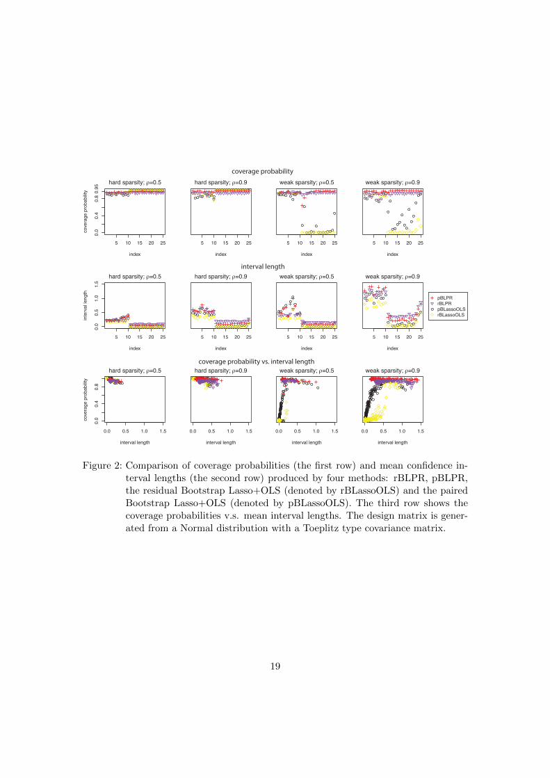
We now compare the performance of the rBLPR and pBLPR methods with that ofthe Bootstrap Lasso+OLS method. Figure 2 shows the comparison results in terms ofcoverage probabilities and mean confidence interval lengths for the Normal distributeddesign matrix in Scenario 1 with a Toeplitz type covariance matrix corresponding toρ = 0.5 or 0.9 and β0 with hard or weak sparsity. For other design matrices, theconclusions are similar. We see that the rBLPR and pBLPR have similar performance,while the latter performs slightly better; therefore we will only present the results forpBLPR in the following contents. In the hard sparsity cases, all the methods work verywell. In the weak sparsity cases, however, the Bootstrap Lasso+OLS method gives verypoor coverage probabilities (less than 50% for 95% confidence intervals) for the small butnon-zero elements of β0. The reason is that these elements are seldom selected by theLasso and therefore a large proportion of their Bootstrap Lasso+OLS estimates are 0,producing non-coverage confidence intervals like [0, 0]. The pBLPR method dramaticallyimprove the performance of the Bootstrap Lasso+OLS method: it produces promisingcoverage probabilities at the price of slightly increasing the confidence interval lengths.However, we should note that, for some medium-size components of β0, pBLPR maystill have problems covering true values even when design matrices are generated from anormal distribution (The coverage probability for one particular such component is only63%). This is because the Lasso cannot identify these medium-size components withhigh probability.

4.4. Comparison of Bootstrap LPR and de-sparsified methods

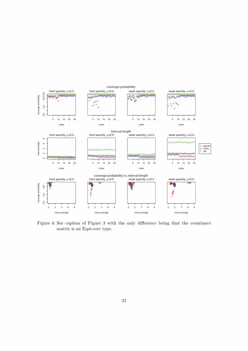
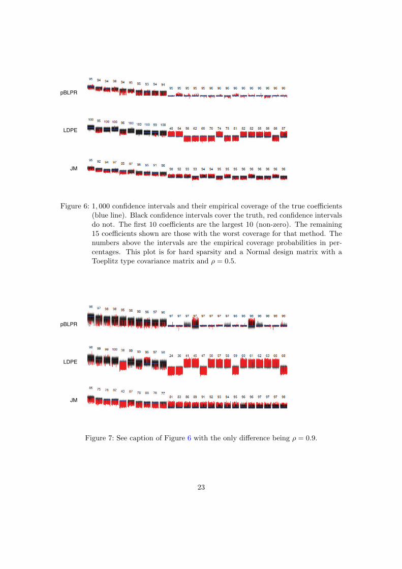
Figures 3, 4 and 5 show the comparison results of pBLPR with LDPE [29] and JM [14],under a Normal design matrix with a Toeplitz type covariance matrix or an Equi.corrtype covariance matrix, or under a t2 distributed design matrix with a Toeplitz typecovariance matrix, respectively. From Figure 3, we see that the pBLPR gives promisingresults. It has overall good performance for large and small components of β0 as com-pared with LDPE and JM, and in some cases it outperforms the other two by producingconfidence intervals with on average 50% shorter lengths (see the comparison results inthe Appendix Tables 1, 2, 3 and 4, which show the mean coverage probabilities and themean lengths of the confidence intervals for large coefficients and small including zerocoefficients, respectively). When the predictors have high correlations (see the results for= 0.9), pBLPR gives confidence intervals with higher coverage probabilities for large co-efficients, and for small and zero coefficients, it gives shorter confidence interval lengthswith good coverage probabilities. Following the evaluation scheme in [9], we also showmore details of the comparison results in Figures 6 - 9, which display the 1, 000 confi-dence intervals and their empirical coverage of the true coefficients (blue line) for threemethods: pBLPR, LDPE, and JM. The black and red colors in these figures are usedto indicate whether confidence intervals cover the truth or not. The first 10 coefficientsare the 10 largest (in absolute values) non-zero coefficients. For each method, the 15

18

5 10 15 20 25

0.0

0.4

0.8

hard sparsity; ρ=0.5

index

cove

rag

e p

rob

ab

ility

5 10 15 20 25


index

5 10 15 20 25

weak sparsity; ρ=0.5

index

5 10 15 20 25


index

5 10 15 20 25

0.0

0.5

1.0

1.5


index

inte

rva

l le

ng

th

5 10 15 20 25


index

5 10 15 20 25


index

5 10 15 20 25


index

0.0 0.5 1.0 1.5

0.0

0.4

0.8


interval length

cove

rag

e p

rob

ab

ility

0.0 0.5 1.0 1.5


interval length

0.0 0.5 1.0 1.5


interval length

0.0 0.5 1.0 1.5


interval length

pBLPR rBLPR pBLassoOLS rBLassoOLS

0.9

5

coverage probability

interval length

coverage probability vs. interval length

Figure 2: Comparison of coverage probabilities (the first row) and mean confidence in-terval lengths (the second row) produced by four methods: rBLPR, pBLPR,the residual Bootstrap Lasso+OLS (denoted by rBLassoOLS) and the pairedBootstrap Lasso+OLS (denoted by pBLassoOLS). The third row shows thecoverage probabilities v.s. mean interval lengths. The design matrix is gener-ated from a Normal distribution with a Toeplitz type covariance matrix.

19

5 10 15 20 25

0.0

0.4

0.8


index

cove

rag

e p

rob

ab

ility

5 10 15 20 25


index

5 10 15 20 25


index

5 10 15 20 25


index

5 10 15 20 25

0.0

0.5

1.0

1.5


index

inte

rva

l le

ng

th

5 10 15 20 25


index

5 10 15 20 25


index

5 10 15 20 25


index

0.0 0.5 1.0 1.5

0.0

0.4

0.8


interval length

cove

rag

e p

rob

ab

ility

0.0 0.5 1.0 1.5


interval length

0.0 0.5 1.0 1.5


interval length

0.0 0.5 1.0 1.5


interval length

0.9

5

pBLPR

LDPE

JM


interval length


Figure 3: Comparison of coverage probabilities (the first row) and mean interval lengths(the second row) produced by pBLPR, LDPE and JM. The third line showsthe coverage probabilities v.s. mean interval lengths. The design matrix isgenerated from a Normal distribution with a Toeplitz type covariance matrix.

zero (Figures 6 and 7) or small but non-zero (Figures 8 and 9) coefficients shown arethose with the worst empirical coverage probabilities. The numbers above confidenceintervals are the empirical coverage probabilities in percentages. These figures clearlyshow the advantegeous performance of the pBLPR in constructing confidence intervalsfor a broad range of coefficients.

Under a Normal design matrix with an Equi.corr type covariance matrix (see Figure 4),the JM method does not work well when ρ = 0.9, because it dramatically overestimatesthe noise variance. Our method also has unsatisfactory performance in terms of coverageprobabilities for large coefficients, because the Lasso cannot correctly select the largepredictors due to the strong collinearity among the predictors. Under a t2 design matrix,Figure 5 shows that no methods performs well, leaving large space for improvement. Forother covariance structures, the comparison results are similar to those for the Normaldesign with a Toeplitz type covariance matrix (see Figures 14 and 15 in the Appendix).

In addition, we also compare the bias, standard deviation (SD) and root-mean square

20

5 10 15 20 25

0.0

0.4

0.8


index

cove

rag

e p

rob

ab

ility

5 10 15 20 25


index

5 10 15 20 25


index

5 10 15 20 25


index

5 10 15 20 25

02

46

8


index

inte

rva

l le

ng

th

5 10 15 20 25


index

5 10 15 20 25


index

5 10 15 20 25


index

0 2 4 6 8

0.0

0.4

0.8


interval length

cove

rag

e p

rob

ab

ility

0 2 4 6 8


interval length

0 2 4 6 8


interval length

0 2 4 6 8


interval length

0.9

5


interval length


pBLPR

LDPE

JM

Figure 4: See caption of Figure 3 with the only difference being that the covariancematrix is an Equi.corr type.

21

5 10 15 20 25

0.0

0.4

0.8


index

cove

rag

e p

rob

ab

ility

5 10 15 20 25


index

5 10 15 20 25


index

5 10 15 20 25


index

5 10 15 20 25

0.0

1.0

2.0

index

inte

rva

l le

ng

th

5 10 15 20 25

index

5 10 15 20 25

index

5 10 15 20 25

index

0.0 0.5 1.0 1.5 2.0

0.0

0.4

0.8

interval length

cove

rag

e p

rob

ab

ility

0.0 0.5 1.0 1.5 2.0

interval length

0.0 0.5 1.0 1.5 2.0

interval length

0.0 0.5 1.0 1.5 2.0

interval length

pBLPR

LDPE

JM

0.9

5


interval length


hard sparsity; ρ=0.5 hard sparsity; ρ=0.9 weak sparsity; ρ=0.5 weak sparsity; ρ=0.9

hard sparsity; ρ=0.5 hard sparsity; ρ=0.9 weak sparsity; ρ=0.5 weak sparsity; ρ=0.9

Figure 5: See caption of Figure 3 with the only difference being the type of design matrix.In this plot, the design matrix is generated from t2 distribution with a Toeplitztype covariance matrix.

22

pBLPR

LDPE

JM

Figure 6: 1, 000 confidence intervals and their empirical coverage of the true coefficients(blue line). Black confidence intervals cover the truth, red confidence intervalsdo not. The first 10 coefficients are the largest 10 (non-zero). The remaining15 coefficients shown are those with the worst coverage for that method. Thenumbers above the intervals are the empirical coverage probabilities in per-centages. This plot is for hard sparsity and a Normal design matrix with aToeplitz type covariance matrix and ρ = 0.5.

pBLPR

LDPE

JM

Figure 7: See caption of Figure 6 with the only difference being ρ = 0.9.

23

pBLPR

LDPE

JM

Figure 8: See caption of Figure 6 with the only difference being weak sparsity.

pBLPR

LDPE

JM

Figure 9: See caption of Figure 6 with the only differences being weak sparsity andρ = 0.9.

24

5 10 15 20 25

0.0

0.2

0.4


Index

ab

so

lute

bia

s

5 10 15 20 25


Index

5 10 15 20 25


Index

5 10 15 20 25


Index

5 10 15 20 25

0.0

0.2

0.4


Index

sta

nd

ard

devia

tio

n

5 10 15 20 25


Index

5 10 15 20 25


Index

5 10 15 20 25


Index

5 10 15 20 25

0.0

0.2

0.4

0.6


Index

roo

t−m

ea

n s

qu

are

d e

rro

r

5 10 15 20 25


Index

5 10 15 20 25


Index

5 10 15 20 25


Index

Lasso

LPR

LDPE

JM

absolute bias

standard deviation

root-mean squared error

Figure 10: Comparison of bias, standard deviation and root-mean squared error. Thedesign matrix is generated from the Normal distribution with a Toeplitz typecovariance matrix.

error (RMSE) of the de-sparsified estimators and the LPR estimator to see to whatextent do these methods reduce the Lasso bias. Figure 10 shows these results. We foundthat, compared with LDPE and JM, the LPR estimator has smaller biases (99% and72% smaller on average than LDPE and JM, respectively) for almost all coefficients butthe LPR estimator has larger SDs (30% and 62% larger on average than LDPE and JM,respectively) for large coefficients. Overall, LPR has 60% smaller RMSE than LDPE but42% larger RMSE than JM. Another interesting finding is that although de-sparsifiedestimators can dramatically decrease the biases of the Lasso by more than 40% for largeβ∗j ’s, they could increase the biases more than twice for small or zero β∗j ’s.

4.5. Robustness to signal-to-noise ratios

Figure 11 shows the comparison results under varying signal-to-noise ratios (SNRs). Wecan see that the coverage performance of the de-sparsified methods is more robust toSNR changes. On the other hand, the pBLPR method works well when SNR is high(say, larger than 5), but it may have low coverage probabilities for nonzero coefficients

25

5 10 15 20 25

0.3

0.5

0.7

0.9

SNR=0.5

index

cove

rag

e p

rob

ab

ility

5 10 15 20 25

SNR=1

index

5 10 15 20 25

SNR=5

index

5 10 15 20 25

SNR=10

index

5 10 15 20 25

0.0

0.5

1.0

1.5

SNR=0.5

index

inte

rva

l le

ng

th

5 10 15 20 25

SNR=1

index

5 10 15 20 25

SNR=5

index

5 10 15 20 25

SNR=10

index

0.0 0.5 1.0 1.5

0.0

0.4

0.8

SNR=0.5

interval length

cove

rag

e p

rob

ab

ility

0.0 0.5 1.0 1.5

SNR=1

interval length

0.0 0.5 1.0 1.5

SNR=5

interval length

0.0 0.5 1.0 1.5

SNR=10

interval length

pBLPR

LDPE

JM

0.9

5


interval length


Figure 11: Comparison of coverage probabilities (first row) and mean interval lengths(second row) produced by pBLPR, LDPE and JM when SNR changes. Thethird row shows the coverage probabilities v.s. mean interval lengths. Thedesign matrix is generated from the Normal distribution with a Toeplitz typecovariance matrix and ρ = 0.5.

when SNR is low. This is reasonable because the Lasso cannot correctly identify thetrue nonzero coefficients with high probability when SNR is low. The pBLPR methoddepends more on the model selection performance of the Lasso, but it has much shorter(more than 20% in average) confidence interval lengths for the zero coefficients evenwhen SNR is low.

4.6. Comparison of different methods under the misspecified model

Figure 12 compares the performance of pBLPR, LDPE and JM under the misspecifiedlinear model. The pBLPR performs similarly to LDPE and JM in terms of coverageprobabilities while it produces more than 50% (on average) shorter confidence intervals.

26

0 20 40 60 80 100

0.0

0.2

0.4

0.6

0.8

1.0

SNR=1

index

co

ve

rag

e p

rob

ab

ility

pBLPR

LDPE

JM

0 20 40 60 80 100

0.0

0.2

0.4

0.6

0.8

1.0

SNR=5

index

co

ve

rag

e p

rob

ab

ility

0 20 40 60 80 100

0.0

0.2

0.4

0.6

0.8

1.0

SNR=10

index

co

ve

rag

e p

rob

ab

ility

0 20 40 60 80 100

0.0

0.5

1.0

1.5

2.0

SNR=1

index

inte

rva

l le

ng

th

0 20 40 60 80 100

0.0

0.5

1.0

1.5

2.0

SNR=5

index

inte

rva

l le

ng

th

0 20 40 60 80 100

0.0

0.5

1.0

1.5

2.0

SNR=10

index

inte

rva

l le

ng

th

Figure 12: Comparison of coverage probabilities and mean interval lengths produced bypBLPR, LDPE and JM. The results is based on data simulated from themisspecified linear model (20) - (21) .

27

Table 1: Mean coverage probabilities over large β0j ’s (first 10 largest in absolute value).

Normal design, Toeplitzβ0 ρ rBLPR pBLPR rBLassoOLS pBLassoOLS rBLasso pBLasso LDPE JM

hard .5 .94 .94 .94 .91 .85 .30 .99 .94hard .9 .90 .97 .90 .87 .83 .31 .92 .77weak .5 .94 .94 .94 .90 .83 .27 .95 .90weak .9 .89 .96 .87 .84 .82 .32 .88 .73

Normal design, Exponential decayhard .5 .94 .93 .94 .89 .84 .26 .98 .94hard .9 .94 .93 .94 .88 .83 .25 .99 .95weak .5 .94 .93 .94 .88 .80 .20 .93 .86weak .9 .94 .94 .94 .88 .80 .19 .91 .87

Normal design, Equal correlationhard .5 .78 .87 .71 .60 .65 .40 .90 .98hard .9 .46 .66 .20 .40 .19 .33 .90 1.00weak .5 .79 .82 .67 .48 .59 .33 .84 .96weak .9 .34 .57 .15 .34 .15 .28 .88 1.00

t2 design, Toeplitzhard .5 .65 .53 .39 .45 .23 .03 .78 .10hard .9 .80 .89 .64 .77 .46 .10 .73 .08weak .5 .41 .53 .33 .47 .16 .09 .63 .35weak .9 .74 .51 .20 .46 .13 .20 .64 .30

fMRI designβ0 SNR rBLPR pBLPR rBLassoOLS pBLassoOLS rBLasso pBLasso LDPE JM

hard 1 .68 .76 .36 .61 .26 .37 .95 .94hard 5 .78 .90 .73 .75 .63 .45 .92 .91hard 10 .86 .93 .84 .79 .73 .46 .92 .90weak 1 .63 .75 .30 .59 .22 .36 .95 .97weak 5 .83 .93 .73 .69 .60 .43 .91 .90weak 10 .91 .96 .88 .75 .79 .44 .90 .90

28

Table 2: Mean confidence interval lengths over large β0j ’s (first 10 largest in absolute

value).


hard .5 .24 .27 .18 .27 .15 .20 .37 .23hard .9 .57 .60 .36 .47 .30 .35 .59 .34weak .5 .44 .61 .33 .65 .28 .39 .64 .39weak .9 1.20 1.30 .81 1.04 .65 .76 1.02 .65


Normal design, Equal correlationhard .5 .53 .61 .38 .51 .34 .44 .48 .75hard .9 .94 .94 .33 .49 .32 .44 1.01 3.45weak .5 .99 1.18 .72 .94 .62 .81 .86 1.55weak .9 1.59 1.52 .49 .74 .5 .68 1.84 6.44

t2 design, Toeplitzhard .5 .79 .61 .24 .42 .14 .27 .51 .46hard .9 1.20 1.11 .45 .64 .23 .39 .62 .41weak .5 1.25 1.03 .40 .76 .16 .47 .9 .87weak .9 2.63 1.89 .54 .96 .22 .51 1.33 1.11


hard 1 1.42 1.32 .57 .69 .38 .48 1.40 1.18hard 5 .87 .89 .46 .63 .38 .48 .63 .60hard 10 .66 .71 .37 .53 .32 .42 .44 .43weak 1 2.79 2.50 .86 1.17 .61 .82 2.56 2.20weak 5 1.89 1.89 .89 1.15 .72 .91 1.15 1.12weak 10 1.45 1.53 .73 1.09 .63 .83 .81 .80

29

Table 3: Mean coverage probabilities over small β0j ’s (except first 10 largest in absolute

value).


hard .5 .94 .97 1.00 1.00 .96 1.00 .98 .99hard .9 .93 .99 1.00 1.00 .97 1.00 .96 1.00weak .5 .94 .98 .01 .06 .36 .33 .98 .99weak .9 .93 .99 .03 .15 .20 .35 .96 1.00

Normal design, Exponential decayhard .5 .94 .97 1.00 1.00 .96 1.00 .98 .99hard .9 .94 .97 1.00 1.00 .96 1.00 .96 1.00weak .5 .94 .98 .00 .06 .42 .32 .98 .99weak .9 .94 .98 .01 .05 .42 .31 .97 1.00

Normal design, Equal correlationhard .5 .92 .98 .98 1.00 .98 1.00 .95 1.00hard .9 .93 .98 .98 1.00 .98 1.00 .94 1.00weak .5 .91 .99 .16 .37 .07 .46 .95 1.00weak .9 .93 .97 .07 .25 .04 .35 .94 1.00

t2 design, Toeplitzhard .5 .97 .95 .99 1.00 .99 1.00 .93 1.00hard .9 .94 .98 .99 1.00 .98 1.00 .91 1.00weak .5 .97 .95 .05 .06 .07 .10 .92 1.00weak .9 .96 .97 .04 .09 .05 .13 .9 1.00


hard 1 .93 .98 .99 1.00 .97 1.00 .96 .99hard 5 .93 .98 .99 1.00 .97 1.00 .96 .99hard 10 .93 .98 .99 1.00 .98 1.00 .96 .99weak 1 .93 .98 .05 .22 .05 .35 .96 .99weak 5 .92 .99 .08 .27 .07 .42 .96 1.00weak 10 .92 .99 .07 .26 .07 .44 .96 1.00

30

Table 4: Mean confidence interval lengths over small β0j ’s (except first 10 largest in

absolute value).


hard .5 .09 .05 .00 .01 .01 .02 .38 .23hard .9 .20 .12 .02 .03 .03 .03 .61 .35weak .5 .16 .10 .00 .02 .03 .04 .66 .40weak .9 .39 .24 .04 .06 .05 .06 1.04 .66


Normal design, Equal correlationhard .5 .27 .17 .07 .05 .06 .05 .49 .76hard .9 .75 .46 .13 .10 .12 .09 1.03 3.45weak .5 .49 .34 .15 .12 .12 .10 .87 1.56weak .9 1.36 .83 .22 .18 .23 .17 1.86 6.44

t2 design, Toeplitzhard .5 .53 .24 .02 .03 .01 .02 .54 .51hard .9 .56 .31 .04 .05 .02 .03 .60 .43weak .5 .88 .39 .03 .05 .02 .03 .90 .90weak .9 1.86 .83 .06 .08 .02 .04 1.33 1.12


hard 1 .83 .5 .08 .09 .08 .08 1.40 1.17hard 5 .37 .23 .04 .05 .05 .05 .63 .58hard 10 .26 .16 .03 .03 .04 .04 .44 .42weak 1 1.63 1.01 .19 .18 .15 .15 2.54 2.21weak 5 .75 .50 .12 .12 .10 .10 1.13 1.13weak 10 .52 .36 .07 .09 .08 .08 .80 .81

31

5. Real data illustration

In this section, we demonstrate the performance of our method on a real fMRI (functionalMagnetic Resonance Imaging) data set and compare its performance with the two de-sparsified methods LDPE and JM. The fMRI data were provided by the Gallant Lab atUC Berkeley [15]. The fMRI recorded measurements of blood oxygen level-dependentactivity at 1331 discretized 3D brain volumes (2 × 2 × 2.5 millimeters): cube-like unitscalled voxels. We use a sub-data set focusing on the responses in the ninth voxel locatedin the brain region responsible for visual functions. A single human subject was shownpictures of everyday objects, such as trees, stars, etc. Every picture was a 128 pixelby 128 pixel gray scale image, which was reduced to a vector of length 10921 throughthe following procedure: (1) using Gabor transform of the gray image to generate localcontrast energy features Zj , and (2) taking non-linear transformation Xj = log(1 +√Zj), j = 1, ..., 10921. Training and validation data sets were collected during the

experiment. There were 1750 natural images in the training data consisting of a designmatrix of dimensions 1750× 10921. And the validation data set contained responses to120 natural images9.

5.1. Data processing and pseudo-true (parameter) values

After reading the training data set into R, we calculate the variance of each feature(column) in X and delete those columns whose variances are ≤ 1e−4. Then we have amatrix of dimension 1750× 9076. We further reduce the dimension of the design matrixby correlation screening, i.e., sorting the correlations (Pearson correlation between everyfeature in X and the response Y ) in an decreasing order of absolute values and selectingthe top 500 features with the largest correlation. We use the Lasso+OLS estimate offeature coefficients based on the 1750× 500 design matrix as the pseudo-true parametervalues, denoted by β0. We randomly choose a subset of rows with size n = 200 to create ahigh-dimensional simulation setting and then generate Y from a linear regression modelyi = xTi β

0 + εi. We compare the performance of the pBLPR method with LDPE andJM.

5.2. Confidence intervals

Based on the sub-data set with n = 200 and p = 500, we evaluate the performanceof pBLPR, LDPE and JM in their construction of 95% confidence intervals. The 95%confidence intervals constructed by pBLPR, LDPE and JM cover 95.8%, 97% and 99.6%of the 500 components of β0, respectively. All the three methods cover more than 95% ofthe pseudo-true values and thus have satisfactory performance in terms of coverage. Interms of interval lengths, however, our pBLPR method produces much shorter confidenceintervals than the other two methods do for most of the coefficients, especially thesmall ones. As shown in Figure 13, we illustrate the confidence interval lengths of 100coefficients (44 non-zero coefficients in β0 and 56 randomly chosen zero coefficients)

9We will not use the validation data in this paper.

32

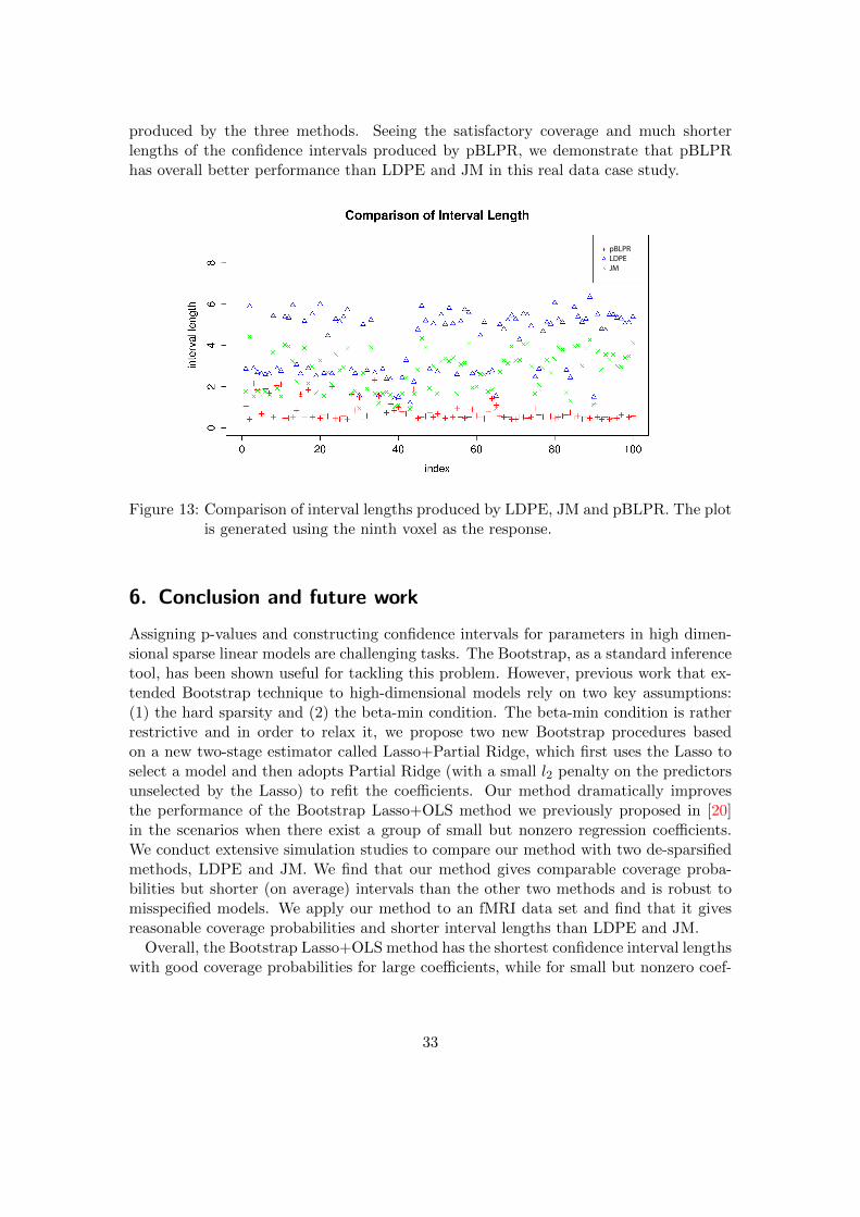
produced by the three methods. Seeing the satisfactory coverage and much shorterlengths of the confidence intervals produced by pBLPR, we demonstrate that pBLPRhas overall better performance than LDPE and JM in this real data case study.

pBLPRLDPEJM

Figure 13: Comparison of interval lengths produced by LDPE, JM and pBLPR. The plotis generated using the ninth voxel as the response.

6. Conclusion and future work

Assigning p-values and constructing confidence intervals for parameters in high dimen-sional sparse linear models are challenging tasks. The Bootstrap, as a standard inferencetool, has been shown useful for tackling this problem. However, previous work that ex-tended Bootstrap technique to high-dimensional models rely on two key assumptions:(1) the hard sparsity and (2) the beta-min condition. The beta-min condition is ratherrestrictive and in order to relax it, we propose two new Bootstrap procedures basedon a new two-stage estimator called Lasso+Partial Ridge, which first uses the Lasso toselect a model and then adopts Partial Ridge (with a small l2 penalty on the predictorsunselected by the Lasso) to refit the coefficients. Our method dramatically improvesthe performance of the Bootstrap Lasso+OLS method we previously proposed in [20]in the scenarios when there exist a group of small but nonzero regression coefficients.We conduct extensive simulation studies to compare our method with two de-sparsifiedmethods, LDPE and JM. We find that our method gives comparable coverage proba-bilities but shorter (on average) intervals than the other two methods and is robust tomisspecified models. We apply our method to an fMRI data set and find that it givesreasonable coverage probabilities and shorter interval lengths than LDPE and JM.

Overall, the Bootstrap Lasso+OLS method has the shortest confidence interval lengthswith good coverage probabilities for large coefficients, while for small but nonzero coef-

33

ficients, the Bootstrap LPR method (rBLPR and pBLPR) has the shortest confidenceinterval lengths with good coverage probabilities. Therefore for practitioners, if they careonly about the confidence intervals for larger coefficients, we recommend the BootstrapLasso+OLS method; if they are also concerned with small coefficients, the BootstrapLPR is a better choice. Moreover, our method has simple implementation and paral-lelization, and it can be easily generalized to models beyond linear models.

As an motivation of the LPR estimator, we extend the model selection consistencyresults of the Lasso from the hard sparsity to the cliff-weak-sparsity case where the truecoefficients β0 can be divided into two groups: “large” components with absolute values� 1/

√n and “small” components with absolute values � 1/

√n, where n is the sample

size. Under the irrepresentable condition and other regularity conditions, we prove thatthe Lasso can correctly select all the large components of β0 while shrinking all the“small” components to exactly zero.

Model misspecification frequently occurs in real data problems. For example, in gene-disease association studies, the joint effects of multiple genes are commonly modeled bylinear models. However, interaction terms between genes not included in models couldalso have significant effects on diseases. In our simulation study we compare our methodwith the de-sparsified methods on a misspecified model, yet our current simulation setupsdo not include all common scenarios encountered in practice. In future work, we planto compare the performance of different inference methods under more types of modelmisspecification.

Multiple testing is another important task in hypothesis testing, which is closely re-lated to confidence interval construction. Several procedures such as the Bonferronicorrection, the Benjamini-Hochberg procedure and the FDR control have been proposedto correct multiple testing in low-dimensional settings. However, these procedures arebased on accurate estimation of p-values of each single test, where small p-values canonly be obtained by large numbers of Bootstrap runs (e.g., a p-value of 0.001 requiresat least 1000 runs), thus imposing too much computational complexity. We leave thecorrection for multiple testing in high-dimensional models to future work.

Acknowledgements

The authors would like to thank the Gallant Lab at UC Berkeley for providing the fMRIdata. The authors thank Simon Walter (UC Berkeley) and Dr. Chad Hazlett (UCLA) fortheir edits and suggestions that have helped clarify the text. The authors also thank Pro-fessor Bin Yu at UC Berkeley for her helpful discussions and comments that have helpedimprove the quality of the paper. Dr. Hanzhong Liu’s research is partially supportedby NSF grants DMS-1613002, DMS-1228246 and AFOSR grant FA9550-14-1-0016. Dr.Jingyi Jessica Li’s research is supported by the Hellman Fellowship, the PhRMA Foun-dation Research Starter Grant in Informatics, NIH/NIGMS grant R01GM120507, andNSF grant NSF grant DMS-1613338.

34

References

[1] Barber R. F., and Candes, E. J. (2015), “Controlling the false discovery rate viaknockoffs,” The Annals of Statistics, 43, 2055-2085.

[2] Berk R., Brown L., Buja A., Zhang K., and Zhao L. (2013), “Valid post-selectioninference,”The Annals of Statististics, 41, 802-837.

[3] Bickel, P. J., and Freedman, D. A. (1983), “Bootstrapping regression models withmany parameters,” In Festschrift for Erich L. Lehmann (P. Bickel, K. Doksum, andJ. Hodges, Jr., eds.) 28-48. Wadsworth, Belmont, Calif.

[4] Buhlmann, P. (2013), “Statistical significance in high-dimensional linear mod-els,”Bernoulli, 19, 1212-1242.

[5] Buhlmann, P., and van de Geer, S. (2011), Statistics for High-Dimensional Data:Methods, Theory and Applications. Springer.

[6] Chatterjee, A., and Lahiri, S. N. (2010), “Asymptotic Properties of the ResidualBootstrap for Lasso Estimators,” Proceedings of the American Mathematical Soci-ety, 138, 4497-4509.

[7] Chatterjee, A., and Lahiri, S. N. (2011), “Bootstrapping Lasso estimators,” Journalof the American Statistical Association, 106, 608-625.

[8] Chatterjee, A., and Lahiri, S. N. (2013), “Rates of convergence of the adaptiveLasso estimators to the oracle distribution and higher order refinements by theBootstrap,” Annals of Statistics, 41, 1232-1259.

[9] Dezeure, R., Buhlmann, P., Meier, L., and Meinshausen, N. (2014), “High-dimensional Inference: Confidence intervals, p-values and R-Software hdi,” Sta-tistical Science, 30, 533-558.

[10] Fan, J., and Lv, J. (2010), “A selective overview of variable selection in high di-mensional feature space,” Statistica Sinica, 20, 101-148.

[11] Hoerl, A. E., and Kennard, R. W. (1970), “Ridge regression: Biased estimation fornonorthogonal problems,” Technometrics, 12, 55-67.

[12] Huang, J., Horowitz, J., and Ma, S. (2008), “Asymptotic properties of bridge es-timators in sparse high-dimensional regression models,” Annals of Statistics, 36,587-613.

[13] Huang, J., S. Ma, and C.-H. Zhang (2008), “Adaptive lasso for sparse high-dimensional regression models,” Statistica Sinica, 18, 1603-1618.

[14] Javanmard, A., and Montanari, A. (2014), “Confidence Intervals and HypothesisTesting for High-Dimensional Regression,” The Journal of Machine Learning Re-search, 15, 2869-2909.

35

[15] Kay, K. N., Naselaris, T., Prenger, R. J., and Gallant, J. L. (2008), “Identifyingnatural images from human brain activity,” Nature, 452, 352-355.

[16] Knight, K. and Fu, W. J. (2000). “Asymptotics for lasso-type estimators,” Annalsof Statistics, 28, 1356-1378.

[17] Lee J. D., Sun D. L., Sun Y., and Taylor, J. E. (2015), “Exact post-selectioninference, with application to the Lasso,” http://arxiv.org/abs/1311.6238.

[18] Lockhart, R., Taylor, J., Tibshirani, R. J., and Tibshirani, R. (2014), “A significancetest for the lasso,” Annals of Statistics, 42, 413-468.

[19] Lopes, M. (2014), “Residual Bootstrap for High-Dimensional Regression withNear Low-Rank Designs,” In: Advances in Neural Information Processing Systems(NIPS), 15, 3239-3247

[20] Liu, H., and Yu, B. (2013), “Asymptotic properties of Lasso+mLS and Lasso+Ridgein sparse high-dimensional linear regression,” Electronic Journal of Statistics, 7,3124-3169.

[21] Meinshausen, N., and Buhlmann, P., (2006), “High dimensional graphs and variableselection with the lasso,” Annals of Statistics, 34, 1436-1462.

[22] Meinshausen, N. (2015), “Group-bound: confidence intervals for groups of variablesin sparse high-dimensional regression without assumptions on the design,” Journalof the Royal Statistical Society Series B, 77, 923-945.

[23] Minnier, J., Tian, L., and Cai, T., (2009), “A perturbation method for inference onregularized regression estimates,” Journal of the American Statistical Association,106, 1371-1382.

[24] Negahban, S., Ravikumar, P., Wainwright M. J., and Yu, B. (2009), “A unifiedframework for high-dimensional analysis of M -estimators with decomposable regu-larizers,” Statistical Science, 28, 538-557.

[25] Tibshirani, R. (1996), “Regression shrinkage and selection via the lasso,” Journalof the Royal Statistical Society Series B, 58, 267-288.

[26] van de Geer, S., Buhlmann, P., Ritov Y., and Dezeure R. (2014), “On asymptoticallyoptimal confidence regions and tests for high-dimensional models,” The Annals ofStatistics, 42, 1166-1202.

[27] Wainwright M. J. (2009), “Sharp thresholds for high-dimensional and noisy sparsityrecovery using-constrained quadratic programming (Lasso),” Information Theory,IEEE, 55, 2183-2202.

[28] Wasserman, L., and Roeder, K. (2009), “High dimensional variable selection,” An-nals of Statistics, 37, 2178-2201.

36

[29] Zhang C., and Stephanie S. Zhang S. S., (2014), “Confidence intervals for lowdimensional parameters in high dimensional linear models,” Journal of the RoyalStatistical Society Series B, 76, 217-242.

[30] Zhao, P., and Yu, B. (2006), “On Model Selection Consistency of Lasso,” TheJournal of Machine Learning Research, 7, 2541-2563.

A. Theoretical property of the residual Bootstrap LPR(rBLPR)

We will show that under orthogonality condition on the design matrix X and underConditions (1) to (10), rBLPR can consistently estimate the distribution of the LPRestimator.

Condition (11) The design matrix is orthogonal, i.e., (1/n)XTX = I.

Theorem 3 Under conditions (1), (2), (4), (6) - (11), for any u ∈ Rp with ||u||2 = 1and max

1≤i≤n|uTxi| = o(

√n), we have

d∞(L∗n,Ln)→p 0, (22)

where L∗n is the conditional distribution of uTT ∗n =√nuT (β0

rBLPR − βLasso+OLS) given ε,

Ln is the distribution of uTTn =√nuT (βLPR − β0), and d∞ denotes the Kolmogorov-

Simirnov distance (sup norm between the distribution functions).

Remark 3 Theorem 3 shows that, under appropriate conditions, the Kolmogorov-Simirnovdistance of the conditional distribution of uTT ∗n and the distribution of uTTn goes to 0in probability. Thus, the unknown distribution of uTTn can be approximated by the con-ditional distribution of uTT ∗n , which can be estimated by the Bootstrap. Based on theestimated conditional distribution of uTT ∗n , we can construct asymptotically valid con-fidence intervals for the linear combination uTβ0. Specifically, by setting u = ej, wecan construct an asymptotically valid confidence interval for an individual coefficient β∗j ,where ej is a basis vector whose jth element equals 1 and other elements equal 0.

Remark 4 The condition max1≤i≤n

|uTxi| = o(√n) is used to verify the Lindeberg condi-

tion, which is used to prove the asymptotic normality of uTT ∗n and uTTn. In the specialcase when u = ej, this condition is equivalent to max

1≤i≤n|xij | = o(

√n), which is not a

strong condition that is expected to hold in many practical situation.

37

B. Proof of Theorems

B.1. Proof of Theorem 1

We will follow the proof of the sign consistency of the Lasso in paper [30] with modifica-tions when necessary. Before proving Theorem 1, we first state the following Proposition1 which is similar to the Proposition 1 in paper [30].

Proposition 1 Assume Condition (5) holds with a constant η > 0 then

P(

(βLasso)S =s β0S , (βLasso)Sc = 0

)≥ P (An ∩Bn) (23)

forAn =

{|C−1

11 WS | <√n(|β0S | − λ1|C−1

11 sign(β0S)| − |C−1

11 C12β0Sc |)},

Bn ={|C21C

−111 WS −WSc | ≤

√nλ1η − |

√n(C21C

−111 C12 − C22)β0

Sc |},

where

WS =1√nXTS ε, and WSc =

1√nXTScε.

Setting β0Sc = 0, then Proposition 1 gives back to the same proposition in paper [30].

Proof. By Karush-Kuhn-Tucker condition for convex optimization, we obtain the fol-lowing Lemma 1 without giving the proof.

Lemma 1 βLasso is the Lasso estimator defined in (2) if and only if

1

2n

d ‖Y −Xβ‖22dβj

|βj=(βLasso)j= −λ1 sign

((βLasso)j

)for j s.t. (βLasso)j 6= 0,

1

2n

∣∣∣∣∣d ‖Y −Xβ‖22dβj|βj=(βLasso)j

∣∣∣∣∣ ≤ λ1 for j s.t. (βLasso)j = 0.

It is easy to obtain

1

2n

d ‖Y −Xβ‖22dβ

= − 1

nXT (Y −Xβ) = C(β − β0)− 1

nXT ε, where, C =

1

nXTX.

Then by definition of the Lasso (2) and Lemma 1, if there exist β = (βTS , 0TSc)T , the

following holds,

√nC11(β − β0)S −

√nC12β

0Sc −XT

S ε/√n = −

√nλ1 sign(β0

S), (24)

−√nλ11 ≤

√nC21(β − β0)S −XT

Scε/√n−√nC22β

0Sc ≤

√nλ11, (25)

|(β − β0)S | < |β0S |, (26)

38

then, β is the Lasso solution, i.e., β = βLasso and hence (βLasso)Sc = βSc = 0 andsign((βLasso)S) = sign(βS) = sign(β0

S). Let W = XT ε/√n and WS = XT

S ε/√n, WSc =

XTScε/√n.

Substitute (β−β0)S and bound the absolute values, the existence of such β is impliedby

|C−111 WS | <

√n(|β0S | − λ1|C−1

11 sign(β0S)| − |C−1

11 C12β0Sc |), (27)

|C21C−111 WS −WSc | ≤

√nλ1

(1− |C21C

−111 sign(β0

S)|)− |√n(C21C

−111 C12 − C22

)β0Sc |.(28)

{(27)} coincides with An and {(28)} ⊂ Bn. This proves Proposition 1.To prove Theorem 1, we can follow the proof of Theorem 4 in paper [30], using our

new Proposition 1.First, by Proposition 1, we have

P(

(βLasso)S =s βS , (βLasso)Sc = 0)≥ P (An ∩Bn).

Whereas

1− P (An ∩Bn) ≤ P (Acn) + P (Bcn)

≤s∑i=1

P(|zi| ≥

√n(|β0

i | − λ1bi − hi))

+

p−s∑i=1

P(|ζi| ≥

√nλ1ηi −mi

),

(29)

where z = (z1, . . . , zs)T = C−1

11 WS , ζ = (ζ1, . . . , ζp−s)T = C21C

−111 WS − WSc , b =

(b1, . . . , bs) = |C−111 sign(β0

S))|, h = (h1, . . . , hs) = |C−111 C12β

0Sc | andm = (m1, . . . ,mp−s) =

|√n(C21C

−111 C12 − C22

)β0Sc |. Due to Condition (1), the εi’s are i.i.d. subgaussian ran-

dom variables with mean 0 and variance σ2. Therefore all zi’s and ζi’s are subgaussianrandom variables with mean 0. By simple algebra, we have

E(zzT ) = σ2C−111 and E(ζζT ) = σ2(C22 − C21C

−111 C12).

Therefore,Ez2

i = σ2(C−111 )ii ≤ σ2Λmax(C−1

11 ) ≤ σ2Λ,

where the last inequality is due to Condition (3).

Eζ2i = σ2(C22 − C21C

−111 C12)ii ≤ σ2(C22)ii = σ2,

where the last equality is because of Condition (2).Therefore all zi’s and ζi’s are subgaussian random variables with mean 0 and finite

variance. Hence, there exits a constant c > 0, such that, ∀t > 0, we have,

P (|zi| ≥ t) ≤ 2e−ct2

and P (|ζi| ≥ t) ≤ 2e−ct2.

By the Cauchy-Schwarz inequality and Conditions (3), (4), and (7), we have, ∀i =1, ..., s,

√nλ1|bi| ≤

√nλ1Λmax(C−1

11 )|| sign(β0S)||2 ≤

√s√nλ1Λ = O(n

12n

c1+c4−12 ) = o(n

12n

c3−12 ),

39

where the last inequality holds because c4 < c3 − c1 in Condition (8).By Condition (8),

√nhi = O(1), ∀i = 1, ..., s. Combining with Condition (6), ∀i =

1, ..., s, we have √nλ1|bi|+

√nhi = o(1)n

12β0

i .

Therefore,

s∑i=1

P(|zi| ≥

√n(|β0

i | − λ1,nbi − hi))≤

s∑i=1

P(|zi| ≥ (1 + o(1))n

12 |β0

i |)

≤s∑i=1

P (|zi| ≥ nc32 )

= o(e−nc2

).

(30)

Due to Conditions (8) and (7), mi = o(nc42 ),√nλ1 = O(n

c42 ). Then,

p−s∑i=1

P(|ζi| ≥

√nλ1ηi −mi

)≤

p−s∑i=1

P(|ζi| ≥ O(n

c42 ))

= o(e−nc2

). (31)

Theorem 1 follows immediately.


Proof. We have to check that the residual Bootstrap version10 of Conditions (1) - (7)hold with conditional probability on data (X,Y ) going to 1. For the residual Bootstrapsample, we have

Y ∗rboot = XβLasso+OLS + ε∗.

Conditions (2), (3) and (7) only depend on X and λ1 which are the same for the origi-nal sample (X,Y ) and the Bootstrap sample (X,Y ∗rboot), therefore they obviously hold.We will show one by one the Bootstrap version of Conditions (1), (4) - (8) hold withprobability going to 1. We need the following Lemma.

Lemma 2 Under Conditions (1) - (7), we have for the constant M in Condition (6),

P(||βLasso+OLS − β0||∞ ≤ 2Mn

c1−12

)→ 1. (32)

Lemma 2 bounds element-wise estimation error of the Lasso+OLS estimator whose proofcan be founded in Appendix C.

Now, we can show that residual Bootstrap version of Conditions (1), (4) - (8) holdwith probability going to 1. Under Conditions (1) - (7) and by Theorem 1, the LassoβLasso has sign consistency, i.e.,

P (S = S) = 1− o(e−nc2)→ 1.

10Replacing (β0, ε, Y ) by (βLasso+OLS, ε∗, Y ∗

rboot).

40

In what follows, we will always condition on {S = S}. By Lemma 2, it is easy to showthat

P(

(βLasso+OLS)S =s β0S

)→ 1,

which guarantees that Bootstrap version of Conditions (4) - (8) hold with probabilitygoing to 1. Therefore, we only need to show the Bootstrap version of Condition (1) holdswith probability going to 1, i.e.,

Condition (1*) ε∗i ’s are conditionally i.i.d. mean 0 subgaussian random variables.That is, there exists constant C∗, c∗ > 0 such that

P ∗(|ε∗i | ≥ t) ≤ C∗e−c∗t2 , ∀t ≥ 0 (33)

holds in probability.

The proof is similar to that in paper [20] with modifications accounting for thecliff-weak-sparsity. Let I· denote the indicator function. Note that P ∗(|ε∗i | ≥ t) =

1n

n∑i=1

I|εi−¯ε|≥t, hence, 33 is equivalent to

supt≥0

{1

n

n∑i=1

ec∗t2I|εi−¯ε|≥t

}≤ C∗. (34)

We know that

εi − ¯ε = yi − xTi βLasso+OLS − (y − xT βLasso+OLS)

= xTi β0 + εi − xTi βLasso+OLS − (xTβ0 + ε− xT βLasso+OLS)

= xTi (β0 − βLasso+OLS) + εi − ε (35)

where xTi is the i-th row of X, y = 1n

n∑i=1

yi, ε = 1n

n∑i=1

εi and x = 1n

n∑i=1

xi = 0. It is easy

to see that supt≥0

{1n

n∑i=1

ec∗t2I|εi−µ|≥t

}can be bounded by

1

n

n∑i=1

{supt≥0

{ec

∗t2I|xTi (β0−βLasso+OLS)|≥t/3

}+ sup

t≥0

{ec

∗t2I|ε|≥t/3}

+ supt≥0

{ec

∗t2I|εi|≥t/3}}

.

(36)

We can bound the second and third terms exactly the same way as in paper [20], i.e.,there exist a constant C∗1 > 0, such that for c∗ = 1

36σ2 ,

P

(1

n

n∑i=1

supt≥0

{ec

∗t2I|ε|≥t/3}≤ C∗1

)→ 1. (37)

P

(1

n

n∑i=1

supt≥0

{ec

∗t2I|εi|≥t/3}≤ C∗1

)→ 1. (38)

41

Since the proof is exactly the same, we omit it here. Next, we have to bound the firstterm, which is different from that in paper [20] because of the weaker cliff-weak-sparsityassumption. For the constant D > 0 appearing in Condition (10),

P ( max1≤i≤n

|xTi (β0 − βLasso+OLS)| ≥ 2D)

= P ( max1≤i≤n

|xTi (β0 − βLasso+OLS)| ≥ 2D, S = S) + P ( max1≤i≤n

|xTi (β − βLasso+OLS)| ≥ 2D, S 6= S)

≤ P ( max1≤i≤n

|xTi,S(β0S − (βLasso+OLS)S) + xTi,Scβ0

Sc | ≥ 2D) + P (S 6= S)

≤ P ( max1≤i≤n

|xTi,S(β0S − (βLasso+OLS)S)| ≥ D) + P ( max

1≤i≤n|xTi,Scβ0

Sc | ≥ D) + P (S 6= S)

= P ( max1≤i≤n

|xTi,S(β0S − (βLasso+OLS)S)| ≥ D) + P (S 6= S), (39)

where the last equality is due to Condition (10). By Cauchy-Schwarz inequality andLemma 2, we have,

max1≤i≤n

|xTi,S(β0S − (βLasso+OLS)S)| ≤ max

1≤i≤n||xi,S ||2||β0

S − (βLasso+OLS)S ||2.

Conditional on {S = S}, the Lasso+OLS estimator has the following form:

(βLasso+OLS)S = (XTSXS)−1XT

S Y = β0S + C−1

11 C12β0Sc + (XT

SXS)−1XTS ε; (40)

(βLasso+OLS)Sc = 0.

Therefore, together with Condition (8),

||β0S−(βLasso+OLS)S ||2 ≤ ||C−1

11 C12β0Sc ||2+||(XT

SXS)−1XTS ε||2 = O(

√s/n)+||(XT

SXS)−1XTS ε||2,

Hence, by Condition (10),

max1≤i≤n

|xTi,S(β0S − (βLasso+OLS)S)| ≤ o(n1/4

√s/n) + max

1≤i≤n||xi,S ||2||(XT

SXS)−1XTS ε||2

= o(1) + max1≤i≤n

||xi,S ||2||(XTSXS)−1XT

S ε||2. (41)

It is easy to show that

max1≤i≤n

||xi,S ||2||(XTSXS)−1XT

S ε||2 = op(1), (42)

therefore,

P

(max

1≤i≤n||xi,S ||2||(XT

SXS)−1XTS ε||2 ≥ D

)→ 0.

Hence,

P

(max

1≤i≤n|xTi (β0 − βLasso+OLS)| ≥ 2D

)→ 0. (43)

42

Therefore,

P

(1

n

n∑i=1

supt≥1

{ec


}≤ e36D2c∗

)

≥ P

(max

1≤i≤n|xTi (β0 − βLasso+OLS)| < 2D

)→ 1. (44)

The inequality holds since it is easy to show that{1

n

n∑i=1

supt≥1

{ec


}≤ e36D2c∗

}⊇{

max1≤i≤n

|xTi (β0 − βLasso+OLS)| < 2D

}.

It is clear that1

n

n∑i=1

sup0≤t≤1

{ec


}≤ ec∗ .

Therefore, with probability going to 1, we have

1

n

n∑i=1

supt≥0

{ec


}= max

{1

n

n∑i=1

sup0≤t≤1

{ec


},

1

n

n∑i=1

supt≥1

{ec


}}≤ max

{ec

∗, e36D2c∗

}(45)

Let C∗ = 2C∗1 + max{ec

∗, e36D2c∗

}and combine (45), (37) and (38),

P

(supt≥0

{1

n

n∑i=1

ec∗t2I|εi−¯ε|≥t

}≤ C∗

)→ 1.


Proof. We first show that

√nuT (βLPR − β0) =

1√nuTXT ε+ op(1); (46)

√nuT (β∗rBLPR − βLasso+OLS) =

1√nuTXT ε∗ + op(1). (47)

For an orthogonal design matrix, Conditions (3) and (5) obviously hold. Thus, bothLasso βLasso and the residual Bootstrap Lasso β0

rLasso have model selection consistency.

We can continue our argument by conditioning on {S = S} and {S∗rLasso = S}.Simple algebra gives that, conditional on {S = S}, the LPR estimator has the following

form √nuTS

{(βLPR)S − β0

S

}=

1√nuTSX

TS ε

43

√nuTSc

{(βLPR)Sc − β0

Sc

}=−√nλ2

1 + λ2uTScβ0

Sc +1√nuTScXT

Scε−λ2

1 + λ2

1√nuTScXT

Scε.

The orthogonal design matrix Condition (11) implies that p ≤ n, hence,

||β0Sc ||2 ≤ (p− s)

12 maxs<j≤p

|β0j | ≤ n

12Mn

−1−c12 = Mn

−c12 → 0, (48)

where the second inequality is due to Condition (6). By Cauchy-Schwarz inequality, for||u||2 = 1,

|−√nλ2

1 + λ2uTScβ0

Sc | ≤√n

1

n||u||2||β0

Sc ||2 → 0.

Since

E

(1√nuTScXT

Scε

)2

= σ2uTScC22uSc = σ2||uSc ||22 ≤ σ2,

we have,λ2

1 + λ2

1√nuTScXT

Scε =1

nOp(1) = op(1).

Therefore,√nuT (βLPR − β) =

1√nuTXT ε+ op(1).

Similarly, conditional on {S∗ = S}, we have

√nuTS

{(β∗rBLPR)S − (βLasso+OLS)S

}=

1√nuTSX

TS ε∗

√nuTSc

{(β∗rBLPR)Sc − (βLasso+OLS)Sc

}=

1√nuTScXT

Scε∗ −λ2

1 + λ2

1√nuTScXT

Scε∗.

By Markov inequality,

P ∗(

1√nuTScXT

Scε∗ > t

)≤ 1

t2E∗(

1√nuTScXT

Scε∗)2

=(σ∗)2

t2uTScC22uSc ≤ (σ∗)2

t2,

where (σ∗)2 = 1n

∑ni=1(εi − ¯ε)2 = 1

n

∑ni=1

[xTi (β0 − βLasso+OLS) + εi − ε

]2.

By Strong Law of Large Number, we have

1

n

n∑i=1

(εi − ε)2 → σ2, almost surely. (49)

44

Since

1

n

n∑i=1

[xTi (β0 − βLasso+OLS)

]2

=1

n

n∑i=1

[xTi,S(β0

S − (βLasso+OLS)S) + xTi,Scβ0Sc

]2

≤ 2

{1

n

n∑i=1

[xTi,S(β0

S − (βLasso+OLS)S)]2

+1

n

n∑i=1

(xTi,Scβ0Sc)2

}≤ 2 max

1≤i≤n|xTi,S(β0

S − (βLasso+OLS)S)|2 + 2||βSc ||22

= op(1), (50)

where the last equality holds because of (41), (42) and (48). Combine (49) and (50), wehave

(σ∗)2 →p σ2.

Therefore,λ2

1 + λ2

1√nuTXT

Scε∗ = Op

(1

n

)= op(1),

which implies

√nuT (β0

rBLPR − βLasso+OLS) =1√nuTXT ε∗ + op(1).

The remainder of the proof is to show that both 1√nuTXT ε and 1√

nuTXT ε∗ converge

in distribution to N(0, σ2). We need to check the Linderberg condition for asymptoticnormality.

For deriving asymptotic normality of 1√nuTXT ε, denote v = 1√

nXu = (v1, ..., vn)T

where vk = 1√nxTk u. Then

∑nk=1 v

2k = 1 and s2

n =∑n

k=1E(vkεk)2 =

∑nk=1 v

2kσ

2 = σ2.

The Linderberg condition holds if for any δ > 0,

1

s2n

n∑k=1

v2kE{ε2kI|vkεk|>δsn

}→ 0. (51)

By the assumption max1≤i≤n

|uTxi| = o(√n), we have

max1≤k≤n

|vk| = max1≤k≤n

|xTk u|/√n = o(1).

Therefore,

1

s2n

n∑k=1

v2kE{ε2kI|vkεk|>δsn

}=

1

σ2

n∑k=1

v2kE{ε2kI|vkεk|>δσ

}≤ 1

σ2max

1≤k≤nE{ε2kI|vkεk|>δσ

}≤ 1

σ2E

{ε21I|ε1|>δσ/ max

1≤k≤n|vk|

}= o(1),

45

where the last equality holds since the error terms εi’s are i.i.d. subgaussian randomvariables.

For deriving asymptotic normality of 1√nuTXT ε∗, denote (s∗n)2 =

∑nk=1E

∗(vkε∗k)

2 =

(σ∗)2 and we needs to verify the Linderberg condition, that is, for any δ > 0,

1

(s∗n)2

n∑k=1

v2kE∗{

(ε∗k)2I|vkε∗k|>δs∗n

}=

1

(s∗n)2

n∑k=1

1

n

n∑i=1

v2k(εi − ¯ε)2I|vk(εi−¯ε)|>δs∗n →p 0. (52)

Since (σ∗)2 →p σ2,∑n

k=1 v2k = 1 and

1

(s∗n)2

n∑k=1

1

n

n∑i=1

v2k(εi − ¯ε)2I|vk(εi−¯ε)|>δs∗n ≤

1

(σ∗)2max

1≤i,k≤n(εi − ¯ε)2I|vk(εi−¯ε)|>δσ∗ ,

we only need to show

1

σ2max

1≤i,k≤n(εi − ¯ε)2I|vk(εi−¯ε)|>δσ = op(1).

For any t > 0,

P

(1

σ2max

1≤i,k≤n(εi − ¯ε)2I|vk(εi−¯ε)|>δσ > t

)≤ P

(max

1≤i,k≤n|vk(εi − ¯ε)| > δσ

)= P

(max

1≤k≤n|vk| max

1≤i≤n|(εi − ¯ε)| > δσ

)= P

(max

1≤k≤n|vk| max

1≤i≤n|xTi (β0 − βLasso+OLS)| > 1

3δσ

)+ P

(max

1≤k≤n|vk| max

1≤i≤n|εi| >

1

3δσ

)+P

(max

1≤k≤n|vk||ε| >

1

3δσ

)= op(1), (53)

where the last but second equality holds because of equation (35) and the last equalityis due to (43) and the i.i.d. subgaussian assumption of the error terms εi’s.

C. Proof of Lemmas

C.1. Proof of Lemma 2

Proof. Under Conditions (1) - (7) and by Theorem 1, the Lasso βLasso has model selectionconsistency, i.e.,

P (S = S) = 1− o(e−nc2)→ 1.

Conditional on {S = S}, the Lasso+OLS estimator has the following form:

(βLasso+OLS)S = (XTSXS)−1XT

S Y = β0S + C−1

11 C12βSc + (XTSXS)−1XT

S ε; (54)

46

(βLasso+OLS)Sc = 0.

Therefore,

||βLasso+OLS − β0||∞ ≤ ||C−111 C12β

0Sc ||∞ + ||(XT

SXS)−1XTS ε||∞ + ||β0

Sc ||∞. (55)

By Condition (8), we have ||C−111 C12β

0Sc ||∞ = o(n

c1−12 ). Condition (6) gives ||β0

Sc ||∞ ≤Mn−

1+c12 . Since (XT

SXS)−1XTS ε are subgaussian random variables with covariance ma-

trix σ2

n C−111 , it is not hard to show that

P(||(XT

SXS)−1XTS ε||∞ ≤Mn

c1−12

)→ 1.

Therefore,

P(||βLasso+OLS − β0||∞ ≤ 2Mn

c1−12

)→ 1.

D. Examples related to Condition (8)

We provide three typical examples of design matrices which satisfy or do not satisfyCondition (8).

D.1. Example 1. Orthogonal design

X is orthogonal so that 1nX

TX is an identity matrix. In this case, C11, C22 are identity

matrices and C12 is a zero matrix. As∥∥β0

Sc

∥∥∞ = o

(1√n

), we have∥∥C−1

11 C12β0Sc

∥∥∞ = 0

and ∥∥√n(C21C−111 C12 − C22)β0

Sc

∥∥∞ =

∥∥√nβ0Sc

∥∥∞ = O(1).

Thus, this example satisfies Condition (8).

D.2. Example 2. Exponential decay

In this example, X has the following pattern:

1

nXTX =

1 ρ ρ2 · · · ρp−1

ρ 1 ρ · · · ρp−2

ρ2 ρ 1 · · · ρp−3

......

.... . .

...ρp−1 ρp−2 ρp−3 · · · 1

(56)

In this case,

C11 =

1 ρ ρ2 · · · ρs−1

ρ 1 ρ · · · ρs−2

ρ2 ρ 1 · · · ρs−3

......

.... . .

...ρs−1 ρs−2 ρs−3 · · · 1

(57)

47

Using mathematical induction, we can prove that

(1−ρ2)C−111 =

1 −ρ 0 · · · 0−ρ 1 + ρ2 −ρ · · · 00 −ρ 1 + ρ2 · · · 0...

......

. . ....

0 · · · −ρ 1 + ρ2 −ρ0 0 · · · −ρ 1

, C12 =

ρs ρs+1 · · · ρp−1

ρs−1 ρs · · · ρp−2

......

. . ....

ρ ρ2 · · · ρp−s

Then,

C−111 C12 =

0 0 · · · 0...

.... . .

...0 0 · · · 0

ρ− ρ3 ρ2 − ρ4 · · · ρp−s − ρp−s+2

(58)

As∥∥β0

Sc

∥∥∞ = o

(1√n

), we have∥∥√nC−1

11 C12β0Sc

∥∥∞ ≤

√n(ρ+ ρ2 − ρp−s+1 − ρp−s+2)

∥∥β0Sc

∥∥∞ = O(1).∥∥√n(C21C

−111 C12 − C22)β0

Sc

∥∥∞ ≤

∥∥√nC21C−111 C12β

0Sc

∥∥∞ +

∥∥√nC22β0Sc

∥∥∞∥∥√nC21C

−111 C12β

0Sc

∥∥∞ ≤

√n(ρ2 + ρ3 − ρp−s+2 − ρp−s+3)

∥∥β0Sc

∥∥∞ = O(1)∥∥√nC22β

0Sc

∥∥∞ <

√n

1−ρ∥∥β0

Sc

∥∥∞ = O(1)

Thus, this example satisfies Condition (8).

D.3. Example 3. Equal correlation

1

nXTX =

1 ρ ρ · · · ρρ 1 ρ · · · ρρ ρ 1 · · · ρ...

......

. . ....

ρ ρ ρ · · · 1

(59)

In this case,

C11 =

1 ρ ρ · · · ρρ 1 ρ · · · ρρ ρ 1 · · · ρ...

......

. . ....

ρ ρ ρ · · · 1

, C12 =

ρ ρ · · · ρρ ρ · · · ρρ ρ · · · ρ...

.... . .

...ρ ρ · · · ρ

It is easy to find that 1 = (1, 1, · · · , 1)T is a eigenvector of C11, so that it is also aeigenvector of C−1

11 . We assume that the sum of elements in β0Sc is SumSc .

Thus, ∥∥C−111 C12β

0Sc

∥∥ = ρ1+ρ(s−1)SumSc .

As we do not assume a bound for SumSc , this example does not always satisfy Condition(8).

48

E. Additional simulation results

5 10 15 20 25

0.0

0.4

0.8


index

cove

rag

e p

rob

ab

ility

5 10 15 20 25


index

5 10 15 20 25


index

5 10 15 20 25


index

5 10 15 20 25

0.0

0.5

1.0

1.5


index

inte

rva

l le

ng

th

5 10 15 20 25


index

5 10 15 20 25


index

5 10 15 20 25


index

0.0 0.5 1.0 1.5

0.0

0.4

0.8


interval length

cove

rag

e p

rob

ab

ility

0.0 0.5 1.0 1.5


interval length

0.0 0.5 1.0 1.5


interval length

0.0 0.5 1.0 1.5


interval length

pBLPR

LDPE

JM

0.9

5


interval length


Figure 14: See caption of Figure 3 with the only difference being that the covariancematrix is Exp.decay.

49

5 10 15 20 25

0.0

0.4

0.8

hard sparsity; SNR=1

index

cove

rag

e p

rob

ab

ility

5 10 15 20 25

0.0

0.4

0.8


index

cove

rag

e p

rob

ab

ility

5 10 15 20 25

weak sparsity; SNR=1

index

5 10 15 20 25


index

0 5 10 15 20 25 30

0.0

1.0

2.0

3.0


index

inte

rva

l le

ng

th

0 5 10 15 20 25 30

0.0

1.0

2.0

3.0


index

inte

rva

l le

ng

th

0 5 10 15 20 25 30


index

0 5 10 15 20 25 30


index

0.0 1.0 2.0 3.0

0.0

0.4

0.8


interval length

cove

rag

e p

rob

ab

ility

0.0 1.0 2.0 3.0

0.0

0.4

0.8


interval length

cove

rag

e p

rob

ab

ility

0.0 1.0 2.0 3.0


interval length

0.0 1.0 2.0 3.0


interval length

pBLPR LDPE JM


interval length


0.9

5

Figure 15: See caption of Figure 3 with the only difference being that the design matrixis generated from the fMRI data.

50

F. Algorithm for cv(Lasso+OLS)

Algorithm 3 K-fold Cross Validation based on Lasso+OLS: cv(Lasso+OLS)

Input: Design matrixX, response Y and a sequence of tuning parameter values λ1, ..., λJ ;Number of folds K.

Output: The optimal tuning parameter selected by cv(Lasso+OLS): λoptimal.

1: Randomly divide the data z = (X,Y ) into K roughly equal folds zk, k = 1, ...,K;

2: For each k = 1, ...,K, denote S(k)(λ0) = ∅ and β(k)Lasso+OLS(λ0) = 0.

• Fit the model with parameters λj , j = 1, ..., J to the other K − 1 folds z−k =

z \ zk of the data, giving the Lasso solution path β(k)(λj), j = 1, ..., J and

compute the selected covariates set S(k)(λj) ={l : β

(k)l (λj) 6= 0

}, j = 1, ..., J

on the path;

• For each j = 1, ..., J , compute the Lasso+OLS estimator:

β(k)Lasso+OLS(λj) =

arg min

β: βj=0, ∀j /∈S(k)(λj)

1

2|z−k|∑i∈z−k

(yi − xTi β)2

, if S(k)(λj) 6= S(k)(λj−1),

β(k)Lasso+OLS(λj−1), otherwise;

• Compute the prediction error PE(k) on the kth fold of the data:

PE(k)(λj) =1

|zk|∑i∈zk

(yi − xTi β

(k)Lasso+OLS(λj)

)2;

3: Compute cross validated error CV E(λj), j = 1, ..., J :

CV E(λj) =1

K

K∑k=1

PE(k)(λj);

4: Compute the optimal λ selected by cross validation:

λoptimal = arg minλj : j=1,...,J

CV E(λj);

5: return λoptimal.

51

Documents

A Bootstrap Lasso + Partial Ridge Method to Construct Con ... · lute coe cients from the largest to the smallest, ... 1.Our proposed Bootstrap LPR method relaxes the beta-min condition