Embed Size (px)
Citation preview
Page 1 of 16
PRODUCTION & MANUFACTURING | RESEARCH ARTICLE
A branch-and-bound method to minimize the makespan in a permutation flow shop with blocking and setup timesMauricio Iwama Takano and Marcelo Seido Nagano
Cogent Engineering (2017), 4: 1389638
Takano & Nagano, Cogent Engineering (2017), 4: 1389638https://doi.org/10.1080/23311916.2017.1389638
PRODUCTION & MANUFACTURING | RESEARCH ARTICLE
A branch-and-bound method to minimize the makespan in a permutation flow shop with blocking and setup timesMauricio Iwama Takano1 and Marcelo Seido Nagano2*
Abstract: This work addresses the minimization of the makespan criterion for the permutation flow shop problem with blocking, sequence and machine dependent setup times, which is a problem that has not been studied in previous works. Many papers considered the problem with an unlimited buffer or with the setup time embedded in the processing time of the job. However, considering an unlimited buf-fer may not represent reality in many industries. Additionally, separating the setup time from the processing time allows greater flexibility for production scheduling, thus allowing better time usage and a reduction in the makespan. Two structural properties of the problem are presented: an upper bound for the machine idle time and a lower bound for the machine blocking time. Using these properties, four lower bounds for the makespan are proposed (LBTN1, LBTN2, LBTN3 and LBTN4). Each of the low-er bounds was used in a branch-and-bound algorithm and then compared to each other using a database containing 540 problems. A MILP model is also presented and compared with the best of the branch-and-bound models using a second data-base that consists of 80 different problems. Computational tests are presented, and the comparisons indicate that the proposed lower bounds are promising.
*Corresponding author: Marcelo Seido Nagano, Department of Production Engineering, School of Engineering of São Carlos, University of São Paulo, Av. Trabalhador São-carlense, 400, 13566-590, São Carlos, SP, Brazil E-mails: [email protected], [email protected]
Reviewing editor:Wenjun Xu, Wuhan University of Technology, China
Additional information is available at the end of the article
ABOUT THE AUTHORSMauricio Iwama Takano is an Assistant Professor in the Mechanical Engineering Department, Federal Technological University – Paraná, Brazil. He holds a PhD in Production Engineering at School of Engineering of São Carlos in the University of São Paulo, Brazil. His research interests include integrated process planning and scheduling, flexible job-shop scheduling and intelligent algorithm.
Marcelo Seido Nagano is an Associate Professor at the School of Engineering of São Carlos in the University of São Paulo, Brazil, where is currently hold the position of Head of the Operations Research Group of the Production Engineering Department. Along with your teaching duties, your research interests refer to decision systems and models in industry and services, including a range of decisions related to the design and optimization of processes, production and planning and scheduling, as well as Knowledge Management and Innovation Management as a supporting infrastructure. In these areas, is carried out several research projects and produced a number of refereed publications.
PUBLIC INTEREST STATEMENTWith the advance of the Toyota production system and the lean manufacturing the study of optimization methods to guarantee the best usage of all resources of the system is becoming more and more important. However, optimization methods are not often explored in industries, one of the reasons for that is that the ideal environment assumed in theoretical problems are not sufficiently similar to those found in real industries. This paper considers a very common problem found in industries, which is a production line with limited space for buffering in process material and setup times between products, a problem that was never studied before in any other work. In this paper some optimization methods are proposed for the problem and they are compared between then, showing that the presented methods are very promising.
Received: 13 January 2017Accepted: 04 October 2017First Published: 13 October 2017
© 2017 The Author(s). This open access article is distributed under a Creative Commons Attribution (CC-BY) 4.0 license.
Page 2 of 16
Page 3 of 16
Takano & Nagano, Cogent Engineering (2017), 4: 1389638https://doi.org/10.1080/23311916.2017.1389638
Subjects: Engineering & Technology; Industrial Engineering & Manufacturing; Production Systems; Production Engineering
Keywords: flow shop; blocking; zero buffer; setup times; makespan; lower bound; branch–and-bound; MILP
1. IntroductionThis paper studies the scheduling problem in a permutation flow shop with zero buffer and sequence and machine dependent setup environment, a problem that has not yet been explored in the litera-ture. In the problem, there are n jobs that must be processed by m machines, and all jobs must be processed in all machines in the same flow. The permutation constraint indicates that the process sequence of the jobs must be the same for all machines. In this paper, the setup time is separated from the process time (i.e. anticipatory setup), allowing a machine to be prepared to initiate the pro-cess of a job before the previous machine has finished the process of this job. That is, whenever a machine is not processing any job, it is possible to prepare the machine for the upcoming job in ad-vance, regardless of whether the upcoming job is still being processed by previous machines. This ensures a better flexibility for the scheduling but is only possible if the processed part is not necessary for the setup. The setup time depends on the sequence of the jobs and the machine. In other words, there is a different setup time for each pair of jobs in each machine. In an environment with blocking, there are limited buffers in between the machines; in this paper, we consider a zero buffer constraint. In other words, if machine k finishes the processing of job j and machine k + 1 is not able to receive the job (because it is still processing job j − 1 or is still being set up), the job remains in machine k, thereby blocking it. In this case, machine k is unable to receive the next job of the sequence.
With the advancement of the Toyota production system and lean manufacturing, the buffer size between work stations is becoming increasingly limited. Therefore, studying the limited buffer con-straint is becoming more important (Ronconi, 2005). The flow shop problem with zero buffer can be used to model any flow shop problem with a limited buffer because a unit capacity buffer can be represented by a machine with zero processing time for all jobs (McCormick, Pinedo, Shenker, & Wolf, 1989).
The flow shop with zero buffer and dependent setup time is an underexplored problem. Therefore, a bibliographic review of the flow shop with a blocking problem is presented first. This bibliographic review considers the few works that examine a flow shop with blocking and sequence dependent setup time problem, both with the objective of minimizing the makespan.
Among the most important and pioneering works is that of Gilmore and Gomory (1964). The au-thors solved the one- and two-machine problems by using a one state-variable with 0(N²) simple steps. Reddi and Ramamoorthy (1972) showed that the traditional flow shop problem with only two machines (two work stations) and the blocking constraint can be transformed into a special case of the travelling salesman problem.
Papadimitriou and Kanellakis (1980) proved that the problem with a limited buffer of only one unit between machines is NP-HARD. Hall and Sriskandarajah (1996), based on the results obtained by Papadimitriou and Kanellakis (1980), showed that the traditional flow shop with three work stations and a blocking problem is strongly NP-complete. In the same paper, the authors related the main works developed in the literature.
McCormick et al. (1989) presented a heuristic method denominated Profile Fitting (PF), in which jobs are scheduled in such a way that the idle and blocking times of the machines are minimized.
Leisten (1990) presented two heuristic methods for permutation and non-permutation flow shop problems with limited buffers. The performance measures of the methods used were the maximum use of the buffers and the minimum blocking times. The computational experiments showed that
Page 4 of 16
Takano & Nagano, Cogent Engineering (2017), 4: 1389638https://doi.org/10.1080/23311916.2017.1389638
the adaptation of the traditional Nawaz-Enscore-Ham (NEH) created by Nawaz, Enscore, and Ham (1983), which was originally developed for the unlimited buffer problem, had better performance than did the proposed methods.
Ronconi (2004) addressed the zero buffer problem with the objective of minimizing the makespan. A constructive heuristic method that uses specific characteristics of the problem is presented. The new method, combined with some of the best methods in the literature, was compared to the adapted version of the NEH and presented better results.
Pan and Wang (2012) considered the flow shop with blocking problem, with the objective of mini-mizing the makespan. Initially, the authors presented two constructive heuristic methods, named Weighted Profile Fitting (wPF) and (PW), both of which were based on the Profile Fitting (PF) proce-dure presented by McCormick et al. (1989). They proposed three II phase heuristics (according to Framinan, Gupta, & Leisten, 2004 classification), named PF-NEH, wPF-NEH and PW-NEH, by combin-ing the previous methods with the classic NEH. Finally, using a local search (LS) method based on job insertion, three III phase heuristics (according to Framinan et al., 2004 classification) were devel-oped: PF-NED/LS, wPF-NEH/LS and PW-NEH/LS. The proposed methods were evaluated and compared with other existing methods using the database provided by Taillard (1993). The experiments showed that the proposed methods outperformed all other methods previously presented in the literature. In addition, the III phase methods significantly improved the results obtained by the con-structive methods. The computational tests provided better solutions for 17 large problems from the database.
Ronconi and Armentano (2001) presented branch-and-bound algorithms for the flow shop with blocking problem. It proposed a lower bound for the departure time of the jobs. Thereafter, lower bounds for the total tardiness and makespan were developed.
Pranzo (2004) showed that the Batch scheduling in a two-machine flow shop with limited buffer and sequence independent setup times and removal times can be formulated as a special case of the TSP. It can be solved in polynomial time, depending on the batch size.
Subsequently, Ronconi (2005) presented a branch-and-bound algorithm that used new lower bounds, which advantageously used the nature and structure of the blocking problem. The new method outperformed the method proposed by Ronconi and Armentano (2001) that was adapted for the problem.
Moslehi and Khorasanian (2013) proposed two mixed integer linear programming (MILP), an initial upper bound generator and some lower bounds and dominance rules to be used in a branch-and-bound algorithm to minimize the total completion time in a permutation flow shop problem with zero buffer. The MILP models had some trouble with solving instances with sizes (n, m) equal to (16, 10), (18, 7), and (18, 10). The branch-and-bound model was able to solve 30 of the 120 instances from the Taillard (1993) database.
Chen, Zhou, Li, and Xu (2014) studied a two-stage flow shop problem with batch processing ma-chines, arbitrary release dates and zero buffer, with the objective of minimizing the makespan. A MILP model for the problem was proposed, as was a Hybrid Discrete Differential Evolution (HDDE) algorithm. The proposed algorithm HDDE was compared to the MILP model, a Hybrid Simulated Annealing (HSA) and a Hybrid Genetic Algorithm (HGA). The HDDE algorithm outperformed the other methods in terms of solution quality, robustness, and computational time.
The first work to address the flow shop problem with limited buffer and sequence and machine dependent setup found in the literature is that by Norman (1999). The evaluation criterion used in this work was the minimum makespan. A Tabu search and two adapted constructive heuristics methods (NEH and PF) were presented to solve the problem. A greedy improvement procedure was
Page 5 of 16
Takano & Nagano, Cogent Engineering (2017), 4: 1389638https://doi.org/10.1080/23311916.2017.1389638
added to the constructive heuristics. Overall, 900 problems were generated to evaluate the pro-posed methods, which had varying setup times, buffer sizes and numbers of jobs and machines.
Maleki-Darounkolaei, Modiri, Tavakkoli-Moghaddam, and Seyyedi (2012) developed a MILP model and a Simulated Annealing (SA) for the flow shop problem with three work stations, a sequence-dependent setup time only in the first stage and a blocking time between each stage, with two ob-jectives: to minimize the makespan and the flow time. Problems with more than nine jobs were not solved due to the elevated computational time.
It is important to note that even though two works addressed the problem of blocking with se-quence-dependent setup times, no work was found in the literature that considered the zero buffer among with the sequence and machine dependent setup time in all machines. Therefore, there are no existing methods to solve this problem. In this paper, a branch-and-bound (B&B) algorithm is presented to minimize the makespan in a permutation flow shop environment with zero buffer and sequence and machine dependent setup, with m machines and n jobs. An upper bound for the idle time of the machines and a lower bound and the blocking time of the machines are presented in this work. Then, four lower bounds for the makespan, based on these structural properties of the prob-lem, are presented. The efficiency of the branch-and-bound and of the lower bounds for the makes-pan are tested using several problems that vary in number of jobs and machines. A MILP model is then presented for the problem, and its efficiency is compared with the efficiency of the best of the lower bound models.
This paper is structured as follows. The calculus used to calculate the makespan is presented in Section 2. Two structural properties of the problem (an upper bound for the machine idle time and a lower bound for the blocking time) are presented in Section 3. The branch-and-bound algorithm and the four lower bounds for the makespan are presented in Section 4. The MILP model for the problem is presented in Section 5. The computational tests for the lower bound models and their results are presented in Section 6. The computational tests for the MILP and the best lower bound models and their results are presented in Section 7. Finally, conclusions are presented in Section 8.
2. Makespan calculusIn this section, we describe how to calculate the makespan in a permutation flow shop environment with blocking and sequence and machine dependent setup time. Let � =
{1, 2,… i, j,… m
} be an
arbitrary sequence of jobs, k ={1, 2,… ,m
} be the sequence of available machines, i be the job
that directly precedes job j in the sequence, Pjk be the processing time of the jth job in sequence in machine k, Sijk be the setup time of machine k between the ith and jth jobs in the sequence, S01k be the setup time of machine k before processing the first job in the sequence, Rjk be the completion time of the setup of machine k to the jth job in the sequence, and Cjk be the departure time of the jth job in the sequence in machine k. The makespan is then calculated by the following:
(1)R1k = S01k(k = 1,… ,m
)
(2)Cj1 = max(Rj2, Rj1 + Pj1
) (j = 1,… , n
)
(3)Cjk = max(Rj,k+1, Cj,k−1 + Pjk
)(j = 1,… ,n); (k = 2,… ,m − 1)
(4)Cjm = Cj,m−1 + Pjm(j = 1,… ,n
)
(5)Rjk = Ci,k + Sijk(j = 2,… ,n
);(k = 1,… ,m
)
Page 6 of 16
Takano & Nagano, Cogent Engineering (2017), 4: 1389638https://doi.org/10.1080/23311916.2017.1389638
Initially, the setup completion times of the machines for the first job in the sequence are calcu-lated by Equation (1). Next, the departure times of the first job in all machines are calculated by Equations (2), (3), and (4). Then, Equation (5) is used to calculate the setup completion time of all machines for the following job. Equations (2), (3), and (4) are used again to calculate the departure times of the following job in all machines. The makespan (Cmax) is equal to the departure time of the last job in sequence in the last machine. In other words, Cmax = Cnm.
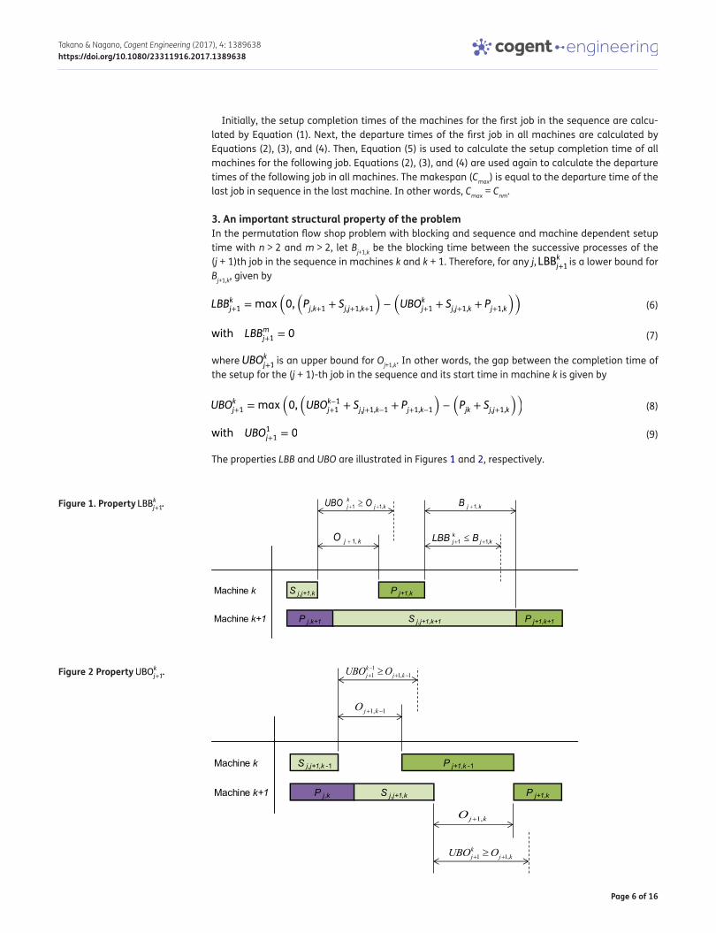
3. An important structural property of the problemIn the permutation flow shop problem with blocking and sequence and machine dependent setup time with n > 2 and m > 2, let Bj+1,k be the blocking time between the successive processes of the (j + 1)th job in the sequence in machines k and k + 1. Therefore, for any j, LBBkj+1 is a lower bound for Bj+1,k, given by
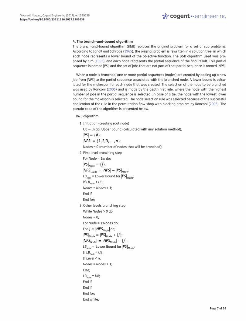
where UBOkj+1 is an upper bound for Oj+1,k. In other words, the gap between the completion time of the setup for the (j + 1)-th job in the sequence and its start time in machine k is given by
The properties LBB and UBO are illustrated in Figures 1 and 2, respectively.
(6)LBBkj+1 = max(0,(Pj,k+1 + Sj,j+1,k+1
)−(UBOkj+1 + Sj,j+1,k + Pj+1,k
))
(7)with LBBmj+1 = 0
(8)UBOkj+1 = max(0,(UBOk−1j+1 + Sj,j+1,k−1 + Pj+1,k−1
)−(Pjk + Sj,j+1,k
))
(9)with UBO1j+1 = 0
Figure 1. Property LBBkj+1.
Figure 2 Property UBOkj+1.
Page 7 of 16
Takano & Nagano, Cogent Engineering (2017), 4: 1389638https://doi.org/10.1080/23311916.2017.1389638
4. The branch-and-bound algorithmThe branch-and-bound algorithm (B&B) replaces the original problem for a set of sub problems. According to Ignall and Schrage (1965), the original problem is rewritten in a solution tree, in which each node represents a lower bound of the objective function. The B&B algorithm used was pro-posed by Kim (1995), and each node represents the partial sequence of the final result. This partial sequence is named |PS|, and the set of jobs that are not part of that partial sequence is named |NPS|.
When a node is branched, one or more partial sequences (nodes) are created by adding up a new job from |NPS| to the partial sequence associated with the branched node. A lower bound is calcu-lated for the makespan for each node that was created. The selection of the node to be branched was used by Ronconi (2005) and is made by the depth first rule, where the node with the highest number of jobs in the partial sequence is selected. In case of a tie, the node with the lowest lower bound for the makespan is selected. The node selection rule was selected because of the successful application of the rule in the permutation flow shop with blocking problem by Ronconi (2005). The pseudo code of the algorithm is presented below.
B&B algorithm
1. Initiation (creating root node)
UB → Initial Upper Bound (calculated with any solution method);
||PS|| ={�}
;
||NPS|| ={1, 2, 3,… ,n
};
Nodes = 0 (number of nodes that will be branched);
2. First level branching step
For Node = 1:n do;
||PS||Node ={j}
;
||NPS||Node = ||NPS|| − ||PS||Node; LBNode = Lower Bound for ||PS||Node; If LBNode < UB;
Nodes = Nodes + 1;
End if;
End for;
3. Other levels branching step
While Nodes > 0 do;
Nodes = 0;
For Node = 1:Nodes do;
For j ∈ ||NPSNode|| do;
||PS||Node = ||PS||Node +{j}
;
||NPSNode|| = ||NPSNode|| −{j}
;
LBNode = Lower Bound for ||PS||Node; If LBNode < UB;
If Level < n;
Nodes = Nodes + 1;
Else;
LBNode = UB;
End if;
End if;
End for;
End while;
Page 8 of 16
Takano & Nagano, Cogent Engineering (2017), 4: 1389638https://doi.org/10.1080/23311916.2017.1389638
4.1. Lower bound for the makespanConsidering a partial sequence |PS|, the lower bound for the makespan is the minimum value of the departure time of the last job from ||NPS|| in the last machine (m). Four lower bounds for the makes-pan were developed for the Fm|prmu, Sijk, block|Cmax problem, considering the lower bound for the blocking (LBBkij). Let PS be the last job in the partial sequence and ||NPS|| be the set of jobs that are not part of the partial sequence. Let S_Si,j,k be the sum of the minimum setup times of the jobs that are not part of the partial sequence in machine k, and let S_LBBi,j,k be the sum of the minimum lower bound for the blocking time of the jobs that are not part of the partial sequence in machine k. S_Si,j,k and S_LBBi,j,k are given by Equations (10) and (11).
The first part of Equation (10) sums the minimum setup times for all jobs that are not part of the partial sequence. The second part of the equation removes the setup time of the last job in the se-quence from S_Si,j,k, as the last job of the sequence is going to be determined in the lower bound equation. A similar method is used to calculate the value of S_LBBi,j,k in Equation (11). Both S_Sni,j,k and S_LBBni,j,k are used to calculate LBTN1, LBTN2, and LBTN4.
Let LW be the processing time summed by the value of the lower bound of the blocking time of the last job in the sequence. The last job in the sequence is the one with the smallest value for the sum of the processing times and the lower bound of the blocking. In other words,
The last job in the sequence is removed from ||NPS||, and the new set of jobs is named ||NPSn||. With this new set, it is possible to calculate S_Sni,j,k, which is the sum of the minimum setup times of the jobs that are not part of the partial sequence and are not the last job in the sequence in machine k. S_LBBni,j,k is the sum of the minimum lower bound for the blocking time of the jobs that are not part of the partial sequence or the last job in the sequence in machine k. We use the following equations:
The first part of Equation (13) sums the minimum setup times for all jobs that are not part of the partial sequence. The second part of the equation removes the setup time of the last job in the se-quence from S_Sni,j,k, as the last job of the sequence is already identified by LW(k). A similar method is used to calculate the value of S_LBBni,j,k in Equation (14). Both S_Sni,j,k and S_LBBni,j,k are used only to calculate LBTN3.
The lower bounds were named LBTN1, LBTN2, LBTN3 and LBTN4 and are obtained by the following equations:
(10)S_Si,j,k =∑
i∈|NPS|∪ PS
(min
(Si,|NPS|,k
))−max
(min
(S|NPS|,|NPS|,k
))
(11)S_LBBi,j,k =
∑
i∈|NPS|∪ PS
(min
(LBBki,|NPS|
))−max
(min
(LBBk|NPS|,|NPS|
))∀k = 1,… ,m − 1
(12)LW(k) = min
(m∑
q=k+1
(P|NPS|,q
)+min
(m∑
q=k+1
(LBB
q
|NPS|,|NPS|
)))∀k = 1,… ,m − 1
(13)S_Sni,j,k =∑
i∈|NPSn|∪ PS
(min
(Si,|NPS|,k
))−max
(min
(S|NPSn|,|NPS|,k
))∀k = 1,… ,m − 1
(14)S_LBBni,j,k =∑
i∈|NPSn|∪ PS
(min
(LBBki,|NPS|
))−max
(min
(LBBk|NPSn|,|NPS|
))∀k = 1,… ,m − 1
(15)
LBTN1(k)= CPS,k + S_Si,j,k +
∑
h∈|NPS|
(Phk
)+ S_LBBki,j +ming∈|NPS|
(m∑
q=k+1
(Pg,q +min
(LBBqg,g
)))∀k = 1,… ,m − 1
Page 9 of 16
Takano & Nagano, Cogent Engineering (2017), 4: 1389638https://doi.org/10.1080/23311916.2017.1389638
The first part of Equations (15), (18), (21), and (24) sum the departure time of the last job in the par-tial sequence (CPS,k), the sum of the setup times of all jobs in ||NPS|| (S_Si,j,k), the sum of the processing times of all jobs in ||NPS|| (
∑h∈�NPS�
�Phk
�), and the sum of the lower bound for the blocking times of all
jobs in ||NPS|| (S_LBBki,j), respectively. The second part of the equations tries to identify the last job in
the sequence and sum the processing times and lower bound for the blocking times in all subse-quent machines.
In Equation (15), the last job in the sequence is the job with the minimum sum of the processing times and the minimum values of the lower bound for the blocking times in all further machines. In Equation (18), the last job in the sequence is the job that has the minimum value for the sum of all processing times in the subsequent machines added to the minimum value of the sum of the lower bound for the blocking times in all subsequent machines. In Equation (21), the last job in the se-quence is job LW, as calculated by Equation (12). Finally, in Equation (24), the departure time of the last job in the sequence is calculated by summing the minimum value of the processing time, added by the value of the minimum lower bound for the blocking time in all subsequent machines.
In Equations (16), (19), (22), and (25), the departure time is calculated by summing the departure time of the last job in the partial sequence (CPS,k), the sum of the setup times of all jobs in ||NPS||
(S_Si,j,k), and the sum of the processing times of all jobs in ||NPS|| �
∑h∈�NPS�
�Phk
��
. The lower bound for
the blocking is not considered in these equations because there is no blocking in the last machine.
(16)LBTN1(m) = CPS,m + S_Si,j,m +∑
h∈|NPS|
(Phm
)
(17)LBTN1 = max1≤k≤m(LBTN1
(k))
(18)
LBTN2(k)= CPS,k + S_Si,j,k +
∑
h∈|NPS|
(Phk
)+ S_LBBki,j +ming∈|NPS|
(m∑
q=k+1
(Pg,q
)+min
(m∑
q=k+1
(LBBqg,g
)))∀k = 1,… ,m − 1
(19)LBTN2(m) = CPS,m + S_Si,j,m +∑
h∈|NPS|
(Phm
)
(20)LBTN2 = max1≤k≤m(LBTN2
(k))
(21)LBTN3(k)= CPS,k + S_Sni,j,k +
∑
h∈|NPS|
(Phk
)+ S_LBBnki,j + LW ∀k = 1,… ,m − 1
(22)LBTN3(m) = CPS,m + S_Si,j,m +∑
h∈|NPS|
(Phm
)
(23)LBTN3 = max1≤k≤m(LBTN3
(k))
(24)
LBTN4(k)= CPS,k + S_Si,j,k +
∑
h∈|NPS|
(Phk
)+ S_LBBki,j +
m∑
q=k+1
(ming∈|NPS|
(Pg,q
)+ming∈|NPS|
(LBBqg,g
))∀k = 1,… ,m − 1
(25)LBTN4(m) = CPS,m + S_Si,j,m +∑
h∈|NPS|
(Phm
)
(26)LBTN4 = max1≤k≤m(LBTN4
(k))
Page 10 of 16
Takano & Nagano, Cogent Engineering (2017), 4: 1389638https://doi.org/10.1080/23311916.2017.1389638
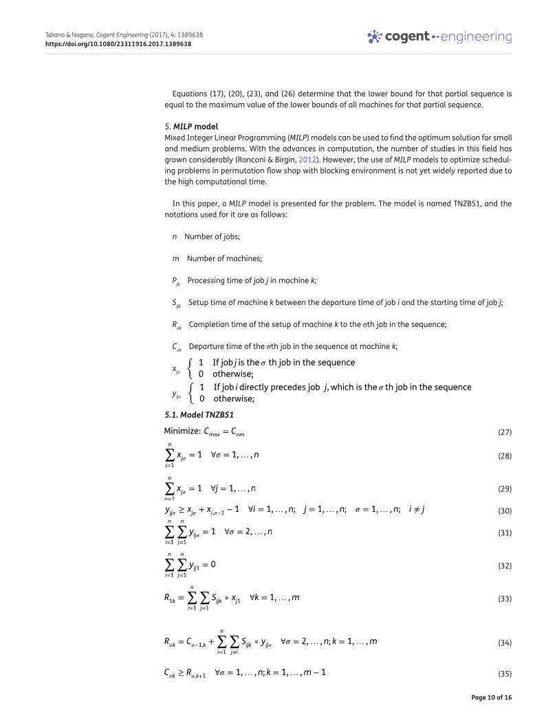
Equations (17), (20), (23), and (26) determine that the lower bound for that partial sequence is equal to the maximum value of the lower bounds of all machines for that partial sequence.
5. MILP modelMixed Integer Linear Programming (MILP) models can be used to find the optimum solution for small and medium problems. With the advances in computation, the number of studies in this field has grown considerably (Ronconi & Birgin, 2012). However, the use of MILP models to optimize schedul-ing problems in permutation flow shop with blocking environment is not yet widely reported due to the high computational time.
In this paper, a MILP model is presented for the problem. The model is named TNZBS1, and the notations used for it are as follows:
n Number of jobs;
m Number of machines;
Pjk Processing time of job j in machine k;
Sijk Setup time of machine k between the departure time of job i and the starting time of job j;
Rσk Completion time of the setup of machine k to the σth job in the sequence;
Cσk Departure time of the σth job in the sequence at machine k;
xjσ {
1 If job j is the � th job in the sequence
0 otherwise;
yijσ {
1 If job i directly precedes job j, which is the � th job in the sequence
0 otherwise;
5.1. Model TNZBS1
(27)Minimize: Cmax = Cnm
(28)n∑
j=1
xj� = 1 ∀� = 1,… ,n
(29)n∑
�=1
xj� = 1 ∀j = 1,… ,n
(30)yij� ≥ xj� + xi,�−1 − 1 ∀i = 1,… ,n; j = 1,… ,n; � = 1,… ,n; i ≠ j
(31)n∑
i=1
n∑
j=1
yij� = 1 ∀� = 2,… ,n
(32)n∑
i=1
n∑
j=1
yij1 = 0
(33)R1k =
n∑
i=1
∑
j=1
Sijk ∗ xj1 ∀k = 1,… ,m
(34)R�k = C�−1,k +
n∑
i=1
∑
j≠i
Sijk ∗ yij� ∀� = 2,… ,n; k = 1,… ,m
(35)C�k ≥ R�,k+1 ∀� = 1,… ,n; k = 1,… ,m − 1
Page 11 of 16
Takano & Nagano, Cogent Engineering (2017), 4: 1389638https://doi.org/10.1080/23311916.2017.1389638
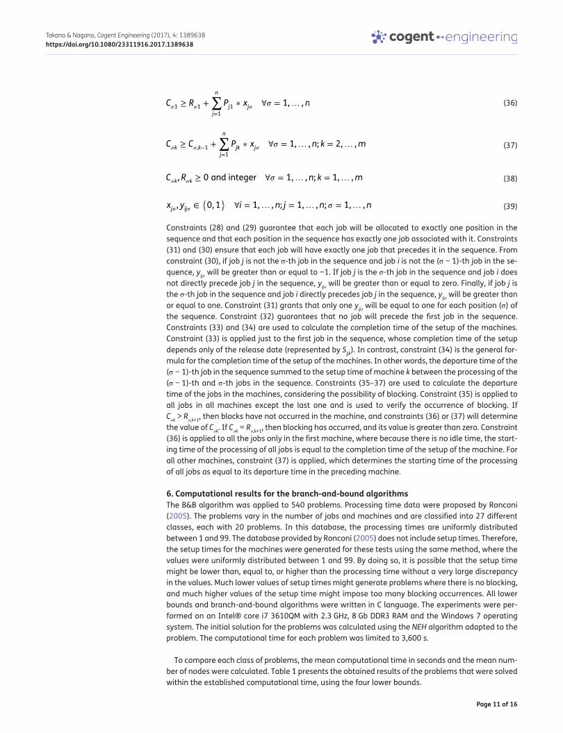
Constraints (28) and (29) guarantee that each job will be allocated to exactly one position in the sequence and that each position in the sequence has exactly one job associated with it. Constraints (31) and (30) ensure that each job will have exactly one job that precedes it in the sequence. From constraint (30), if job j is not the σ-th job in the sequence and job i is not the (σ − 1)-th job in the se-quence, yijσ will be greater than or equal to −1. If job j is the σ-th job in the sequence and job i does not directly precede job j in the sequence, yijσ will be greater than or equal to zero. Finally, if job j is the σ-th job in the sequence and job i directly precedes job j in the sequence, yijσ will be greater than or equal to one. Constraint (31) grants that only one yijσ will be equal to one for each position (σ) of the sequence. Constraint (32) guarantees that no job will precede the first job in the sequence. Constraints (33) and (34) are used to calculate the completion time of the setup of the machines. Constraint (33) is applied just to the first job in the sequence, whose completion time of the setup depends only of the release date (represented by Sjjk). In contrast, constraint (34) is the general for-mula for the completion time of the setup of the machines. In other words, the departure time of the (σ − 1)-th job in the sequence summed to the setup time of machine k between the processing of the (σ − 1)-th and σ-th jobs in the sequence. Constraints (35–37) are used to calculate the departure time of the jobs in the machines, considering the possibility of blocking. Constraint (35) is applied to all jobs in all machines except the last one and is used to verify the occurrence of blocking. If Cσk > Rσ,k+1, then blocks have not occurred in the machine, and constraints (36) or (37) will determine the value of Cσk. If Cσk = Rσ,k+1, then blocking has occurred, and its value is greater than zero. Constraint (36) is applied to all the jobs only in the first machine, where because there is no idle time, the start-ing time of the processing of all jobs is equal to the completion time of the setup of the machine. For all other machines, constraint (37) is applied, which determines the starting time of the processing of all jobs as equal to its departure time in the preceding machine.
6. Computational results for the branch-and-bound algorithmsThe B&B algorithm was applied to 540 problems. Processing time data were proposed by Ronconi (2005). The problems vary in the number of jobs and machines and are classified into 27 different classes, each with 20 problems. In this database, the processing times are uniformly distributed between 1 and 99. The database provided by Ronconi (2005) does not include setup times. Therefore, the setup times for the machines were generated for these tests using the same method, where the values were uniformly distributed between 1 and 99. By doing so, it is possible that the setup time might be lower than, equal to, or higher than the processing time without a very large discrepancy in the values. Much lower values of setup times might generate problems where there is no blocking, and much higher values of the setup time might impose too many blocking occurrences. All lower bounds and branch-and-bound algorithms were written in C language. The experiments were per-formed on an Intel® core i7 3610QM with 2.3 GHz, 8 Gb DDR3 RAM and the Windows 7 operating system. The initial solution for the problems was calculated using the NEH algorithm adapted to the problem. The computational time for each problem was limited to 3,600 s.
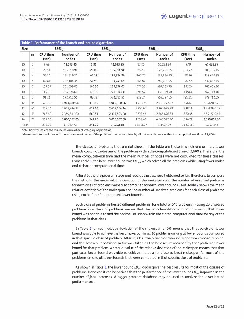
To compare each class of problems, the mean computational time in seconds and the mean num-ber of nodes were calculated. Table 1 presents the obtained results of the problems that were solved within the established computational time, using the four lower bounds.
(36)C�1 ≥ R�1 +
n∑
j=1
Pj1 ∗ xj� ∀� = 1,… ,n
(37)C�k ≥ C�,k−1 +
n∑
j=1
Pjk ∗ xj� ∀� = 1,… ,n; k = 2,… ,m
(38)C�k,R�k ≥ 0 and integer ∀� = 1,… ,n; k = 1,… ,m
(39)xj� , yij� ∈{0, 1
}∀i = 1,… ,n; j = 1,… ,n; � = 1,… ,n
Page 12 of 16
Takano & Nagano, Cogent Engineering (2017), 4: 1389638https://doi.org/10.1080/23311916.2017.1389638
The classes of problems that are not shown in the table are those in which one or more lower bounds could not solve any of the problems within the computational time of 3,600 s. Therefore, the mean computational time and the mean number of nodes were not calculated for these classes. From Table 1, the best lower bound was LBTN2, which solved all the problems while using fewer nodes and a shorter computational time.
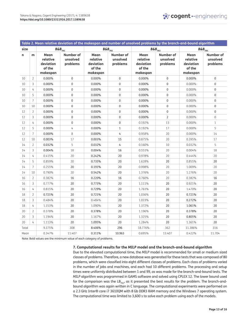
After 3,600 s, the program stops and records the best result obtained so far. Therefore, to compare the methods, the mean relative deviation of the makespan and the number of unsolved problems for each class of problems were also computed for each lower bounds used. Table 2 shows the mean relative deviation of the makespan and the number of unsolved problems for each class of problems using each of the four proposed lower bounds.
Each class of problems has 20 different problems, for a total of 540 problems. Having 20 unsolved problems in a class of problems means that the branch-and-bound algorithm using that lower bound was not able to find the optimal solution within the stated computational time for any of the problems in that class.
In Table 2, a mean relative deviation of the makespan of 0% means that that particular lower bound was able to achieve the best makespan in all 20 problems among all lower bounds compared in that specific class of problem. After 3,600 s, the branch-and-bound algorithm stopped running, and the best result obtained so far was taken as the best result obtained by that particular lower bound for that problem. A smaller value of the relative deviation of the makespan means that that particular lower bound was able to achieve the best (or close to best) makespan for most of the problems among all lower bounds that were compared in that specific class of problems.
As shown in Table 2, the lower bound LBTN2 again gave the best results for most of the classes of problems. However, it can be noticed that the performance of the lower bound LBTN4 improves as the number of jobs increases. A bigger problem database may be used to analyze the lower bound performances.
Table 1. Performance of the branch-and-bound algorithms
Note: Bold values are the minimum value of each category of problems.*Mean computational time and mean number of nodes of the problems that were solved by all the lower bounds within the computational time of 3,600 s.
Size B&BTN1 B&BTN2 B&BTN3 B&BTN4
n m CPU time (sec)
Number of nodes
CPU time (sec)
Number of nodes
CPU time (sec)
Number of nodes
CPU time (sec)
Number of nodes
10 2 6.48 41,633.85 5.91 41,633.85 17.25 50,223.30 6.49 41,633.85
10 3 22.51 104,918.90 20.00 104,918.90 76.23 127,231.35 23.47 109,484.15
10 4 52.24 194,619.30 45.29 193,334.70 202.77 235,896.20 58.66 218,670.85
10 5 64.81 202,104.35 54.93 199,743.05 265.87 249,201.45 74.72 232,867.15
10 7 127.87 302,099.05 105.80 295,858.65 574.30 387,785.70 161.24 380,684.20
10 10 164.93 284,526.60 129.95 270,314.60 691.52 330,139.70 198.64 344,718.40
12 2 91.21 572,712.55 83.32 572,712.55 229.24 659,327.55 91.11 572,712.55
12 3* 423.18 1,903,380.06 376.59 1,903,380.06 1439.92 2,345,772.67 456.63 2,056,967.72
12 4* 727.54 2,648,836.14 629.66 2,618,464.14 2800.96 3,205,695.29 898.19 3,248,940.57
12 5* 785.60 2,389,311.00 660.51 2,337,803.00 2793.43 2,568,676.33 870.45 2,651,519.67
14 2* 594.16 3,890,057.80 542.23 3,890,057.80 1559.40 4,683,547.90 594.78 3,890,057.80
Mean 278.23 1,139,473 241.29 1,129,838 968.2627 1,349,409 312.2164 1,249,842
Page 13 of 16
Takano & Nagano, Cogent Engineering (2017), 4: 1389638https://doi.org/10.1080/23311916.2017.1389638
7. Computational results for the MILP model and the branch-and-bound algorithmDue to the elevated computational time, the MILP model is recommended for small or medium sized classes of problems. Therefore, a new database was generated for these tests that was composed of 80 problems, which were classified into eight different classes of problems. Each class of problems varied in the number of jobs and machines, and each had 10 different problems. The processing and setup times were uniformly distributed between 1 and 99, as was made for the branch-and-bound tests. The MILP algorithm was programmed in GAMS software and solved using CPLEX 12. The lower bound used for the comparison was the LBTN2, as it presented the best results for the problem. The branch-and-bound algorithm was again written in C language. The computational experiments were performed on a 2.3 GHz Inter® core i7 3610QM with 8 Gb DDR3 RAM memory and the Windows 7 operating system. The computational time was limited to 3,600 s to solve each problem using each of the models.
Table 2. Mean relative deviation of the makespan and number of unsolved problems by the branch-and-bound algorithmsize B&BTN1 B&BTN2 B&BTN3 B&BTN4
n m Mean relative
deviation of the
makespan
Number of unsolved problems
Mean relative
deviation of the
makespan
Number of unsolved problems
Mean relative
deviation of the
makespan
Number of unsolved problems
Mean relative
deviation of the
makespan
Number of unsolved problems
10 2 0.000% 0 0.000% 0 0.000% 0 0.000% 0
10 3 0.000% 0 0.000% 0 0.000% 0 0.000% 0
10 4 0.000% 0 0.000% 0 0.000% 0 0.000% 0
10 5 0.000% 0 0.000% 0 0.000% 0 0.000% 0
10 7 0.000% 0 0.000% 0 0.000% 0 0.000% 0
10 10 0.000% 0 0.000% 0 0.000% 0 0.000% 0
12 2 0.000% 0 0.000% 0 0.000% 0 0.000% 0
12 3 0.000% 0 0.000% 0 0.000% 2 0.000% 0
12 4 0.000% 0 0.000% 0 0.192% 13 0.000% 1
12 5 0.000% 4 0.000% 1 0.192% 17 0.000% 5
12 7 0.000% 8 0.000% 4 0.958% 20 0.000% 14
12 10 0.003% 17 0.003% 15 0.875% 20 0.395% 17
14 2 0.032% 5 0.032% 4 0.160% 10 0.032% 5
14 3 0.004% 18 0.004% 16 0.551% 20 0.004% 18
14 4 0.415% 20 0.242% 20 0.978% 20 0.444% 20
14 5 0.859% 20 0.735% 20 1.628% 20 0.855% 20
14 7 0.255% 20 0.191% 20 0.998% 20 1.009% 20
14 10 0.790% 20 0.542% 20 1.376% 20 1.276% 20
16 2 0.382% 16 0.220% 16 0.760% 20 0.382% 16
16 3 0.777% 20 0.773% 20 1.111% 20 0.921% 20
16 4 0.815% 20 0.729% 20 1.761% 20 1.470% 20
18 2 0.721% 20 0.721% 20 1.036% 20 0.721% 20
18 3 0.484% 20 0.484% 20 1.023% 20 0.272% 20
18 4 1.153% 20 1.090% 20 1.372% 20 1.061% 20
20 2 0.378% 20 0.378% 20 1.196% 20 0.378% 20
20 3 1.194% 20 1.167% 20 1.325% 20 0.805% 20
20 4 1.113% 20 1.095% 20 1.284% 20 1.361% 20
Total 9.375% 308 8.406% 296 18.776% 362 11.386% 316
Mean 0.347% 11.407 0.311% 10.963 0.695% 13.407 0.422% 11.704
Note: Bold values are the minimum value of each category of problems.
Page 14 of 16
Takano & Nagano, Cogent Engineering (2017), 4: 1389638https://doi.org/10.1080/23311916.2017.1389638
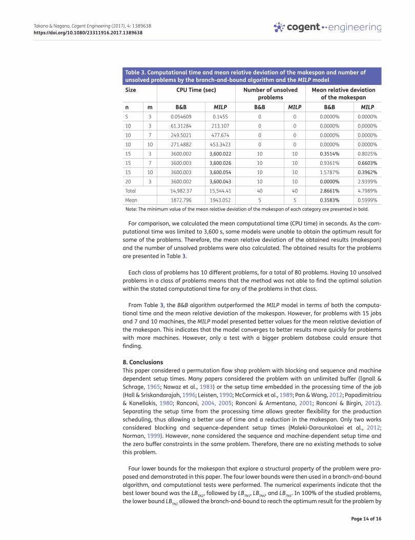
For comparison, we calculated the mean computational time (CPU time) in seconds. As the com-putational time was limited to 3,600 s, some models were unable to obtain the optimum result for some of the problems. Therefore, the mean relative deviation of the obtained results (makespan) and the number of unsolved problems were also calculated. The obtained results for the problems are presented in Table 3.
Each class of problems has 10 different problems, for a total of 80 problems. Having 10 unsolved problems in a class of problems means that the method was not able to find the optimal solution within the stated computational time for any of the problems in that class.
From Table 3, the B&B algorithm outperformed the MILP model in terms of both the computa-tional time and the mean relative deviation of the makespan. However, for problems with 15 jobs and 7 and 10 machines, the MILP model presented better values for the mean relative deviation of the makespan. This indicates that the model converges to better results more quickly for problems with more machines. However, only a test with a bigger problem database could ensure that finding.
8. ConclusionsThis paper considered a permutation flow shop problem with blocking and sequence and machine dependent setup times. Many papers considered the problem with an unlimited buffer (Ignall & Schrage, 1965; Nawaz et al., 1983) or the setup time embedded in the processing time of the job (Hall & Sriskandarajah, 1996; Leisten, 1990; McCormick et al., 1989; Pan & Wang, 2012; Papadimitriou & Kanellakis, 1980; Ronconi, 2004, 2005; Ronconi & Armentano, 2001; Ronconi & Birgin, 2012). Separating the setup time from the processing time allows greater flexibility for the production scheduling, thus allowing a better use of time and a reduction in the makespan. Only two works considered blocking and sequence-dependent setup times (Maleki-Darounkolaei et al., 2012; Norman, 1999). However, none considered the sequence and machine-dependent setup time and the zero buffer constraints in the same problem. Therefore, there are no existing methods to solve this problem.
Four lower bounds for the makespan that explore a structural property of the problem were pro-posed and demonstrated in this paper. The four lower bounds were then used in a branch-and-bound algorithm, and computational tests were performed. The numerical experiments indicate that the best lower bound was the LBTN2, followed by LBTN1, LBTN4, and LBTN3. In 100% of the studied problems, the lower bound LBTN2 allowed the branch-and-bound to reach the optimum result for the problem by
Table 3. Computational time and mean relative deviation of the makespan and number of unsolved problems by the branch-and-bound algorithm and the MILP modelSize CPU Time (sec) Number of unsolved
problemsMean relative deviation
of the makespann m B&B MILP B&B MILP B&B MILP5 3 0.054609 0.1455 0 0 0.0000% 0.0000%
10 3 61.31284 213.107 0 0 0.0000% 0.0000%
10 7 249.5021 477.674 0 0 0.0000% 0.0000%
10 10 271.4882 453.3423 0 0 0.0000% 0.0000%
15 3 3600.002 3,600.022 10 10 0.3514% 0.8025%
15 7 3600.003 3,600.026 10 10 0.9361% 0.6603%
15 10 3600.003 3,600.054 10 10 1.5787% 0.3962%
20 3 3600.002 3,600.043 10 10 0.0000% 2.9399%
Total 14,982.37 15,544.41 40 40 2.8661% 4.7989%
Mean 1872.796 1943.052 5 5 0.3583% 0.5999%
Note: The minimum value of the mean relative deviation of the makespan of each category are presented in bold.
Page 15 of 16
Takano & Nagano, Cogent Engineering (2017), 4: 1389638https://doi.org/10.1080/23311916.2017.1389638
using fewer nodes than the other algorithms used, and it had a 75.08% smaller mean computational time compared to the less effective lower bound (LBTN3). The lower bound LBTN2 was also the one that solved most of the problems within the proposed limit computational time among all proposed lower bounds (18.23% fewer unsolved problems than the lower bound LBTN3). For the problems in which the optimum result was not achieved within the computational time of 3,600 s, it was also the lower bound that obtained the best results (observed by the mean relative deviation of the makespan). However, it is important to note that the performance of the lower bound LBTN4 improved as the num-ber of jobs increased (as observed by the mean relative deviation of the makespan of the bigger classes). Therefore, a larger problem database may be used to validate that finding.
A MILP model was also proposed for the problem. The best lower bound (LBTN2) was compared with the presented MILP model. A new database consisting of 80 problems that varied in the numbers of jobs and machines was created for this comparison. The number of unsolved problems was the same for both methods. However, the computational time required for the branch-and-bound algo-rithm to solve the problem was 3.616% shorter (50.893% if only problems in which “CPU time” was less than 3,600 s) than the computational time required for the MILP model. Additionally, the prob-lems that were not solved within the computational time of 3,600 s had better results when solved by the branch-and-bound algorithm (on average, 40.275% lower than the results obtained by the MILP model). These results show the consistency of the proposed lower bounds for the branch-and-bound algorithm.
It is also important to notice (from Table 3) that the performance of the MILP model tends to im-prove relative to the branch-and-bound algorithm as the number of machines increases. However, the branch-and-bound model tends to improve in relation to the MILP model as the number of jobs increases. For a more accurate result, a larger database is required.
For future works, we propose developing a dominance rule for the branch-and-bound algorithm to reduce the number of nodes. Additionally, the use of heuristics other than NEH, such as MM (Ronconi, 2004), PF, or wPF (Pan & Wang, 2012), can be studied and adapted to the problem as an initial solu-tion for the branch-and-bound. Some other MILP models can be studied and evaluated for their performance.
FundingThe authors acknowledge the partial research support of Conselho Nacional de Desenvolvimento Científico e Tecnológico (CNPq) – Brazil (projects 448161/2014-1, 308047/2014-1).
Author detailsMauricio Iwama Takano1
E-mail: [email protected] ID: http://orcid.org/0000-0002-7622-0283Marcelo Seido Nagano2
E-mails: [email protected], [email protected] ID: http://orcid.org/0000-0002-0239-17251 Federal Technological University - Paraná, Av. Alberto
Carazzai, 1640, 86300-000, Cornélio Procópio, PR, Brazil.2 Department of Production Engineering, School of
Engineering of São Carlos, University of São Paulo, Av. Trabalhador São-carlense, 400, 13566-590, São Carlos, SP, Brazil.
Citation informationCite this article as: A branch-and-bound method to minimize the makespan in a permutation flow shop with blocking and setup times, Mauricio Iwama Takano & Marcelo Seido Nagano, Cogent Engineering (2017), 4: 1389638.
Cover imageSource: Authors
ReferencesChen, H., Zhou, S., Li, X., & Xu, R. (2014). A hybrid differential
evolution algorithm for a two-stage flow shop on batch processing machines with arbitrary release times and blocking. International Journal of Production Research, 52(19), 5714–5734. https://doi.org/10.1080/00207543.2014.910625
Framinan, J. M., Gupta, J. N., & Leisten, R. (2004). A review and classification of heuristics for permutation flow-shop scheduling with makespan objective. Journal of the Operational Research Society, 55, 1243–1255. https://doi.org/10.1057/palgrave.jors.2601784
Gilmore, P. C., & Gomory, R. E. (1964). Sequencing a one state-variable machine: A solvable case of the travelling salesman problem. Operations Research, 12(5), 655–679. https://doi.org/10.1287/opre.12.5.655
Hall, N. G., & Sriskandarajah, C. (1996). A survey of machine scheduling problems with blocking and no-wait in process. Operations Research, 44(3), 510–525. https://doi.org/10.1287/opre.44.3.510
Ignall, E., & Schrage, L. (1965). Application of the branch and bound technique to some flow-shop scheduling problems. Operations Research: The journal of the Operations Research Society of America, 13(3), 400–412. https://doi.org/10.1287/opre.13.3.400
Kim, Y.-D. (1995). Minimizing mean tardiness inpermutation flowshops. European Journal of Operational Research, 85(3), 541–555. https://doi.org/10.1016/0377-2217(94)00029-C
Page 16 of 16
Takano & Nagano, Cogent Engineering (2017), 4: 1389638https://doi.org/10.1080/23311916.2017.1389638
Leisten, R. (1990). Flowshop sequencing problems with limited buffer storage. International Journal of Production Research, 28(11), 2085–2100. https://doi.org/10.1080/00207549008942855
Maleki-Darounkolaei, A., Modiri, M., Tavakkoli-Moghaddam, R., & Seyyedi, I. (2012). A three-stage assembly flow shop scheduling problem with blocking and sequence-dependent set up times. Journal of Industrial Engineering International, 8–26.
McCormick, S. T., Pinedo, M. L., Shenker, S., & Wolf, B. (1989, йил Novembro). Sequencing in an assembly line with blocking to minimize cycle time. Operations Research, 37(6), 925–935. https://doi.org/10.1287/opre.37.6.925
Moslehi, G., & Khorasanian, D. (2013). Optimizing blocking flow shop scheduling problem with total completion time criterion. Computer and Operations Research, 40(7), 1874–1883. https://doi.org/10.1016/j.cor.2013.02.003
Nawaz, M., Enscore, E. E., & Ham, I. (1983). A heuristic algorithm for the m-machine, n-job flow-shop sequencing problem. Omega, 11(1), 91–95. https://doi.org/10.1016/0305-0483(83)90088-9
Norman, B. A. (1999). Scheduling flowshops with finite buffers and sequence-dependent setup times. Computer & Industrial Engineering, 36(1), 163–177. https://doi.org/10.1016/S0360-8352(99)00007-8
Pan, Q. K., & Wang, L. (2012). Effective heuristics for the blocking flowshop scheduling problem with makespan minimization. Omega, 40(2), 218–229. https://doi.org/10.1016/j.omega.2011.06.002
Papadimitriou, C., & Kanellakis, P. (1980). Flow-shop scheduling with limited temporary storage. Journal of the Association
for Computing Machinery, 27(3), 533–549. https://doi.org/10.1145/322203.322213
Pranzo, M. (2004). Batch scheduling in a two-machine flow shop with limited buffer and sequence independent setup times and removal times. European Journal of Operational Research, 153(3), 581–592. https://doi.org/10.1016/S0377-2217(03)00264-9
Reddi, S. S., & Ramamoorthy, C. V. (1972). Flowshop sequencing problem with no wait in process. Operational Research Quarterly, 23(3), 323–331. https://doi.org/10.1057/jors.1972.52
Ronconi, D. P. (2004). A note on constructive heuristics for the flowshop problem with blocking. International Journal of Production Economics, 87(1), 39–48. https://doi.org/10.1016/S0925-5273(03)00065-3
Ronconi, D. P. (2005, Setembro). A branch-and-bound algorithm to minimize the makespan in a flowshop with blocking. Annals of Operations Research, 138(1), 53–65. https://doi.org/10.1007/s10479-005-2444-3
Ronconi, D. P., & Armentano, V. A. (2001). Lower bounding schemes for flowshops with blocking in-process. Journal of the Operational Research Society, 52(11), 1289–1297. https://doi.org/10.1057/palgrave.jors.2601220
Ronconi, D. P., & Birgin, E. G. (2012). Mixed-integer programming models for flowshop scheduling problems minimizing the total earliness and tardiness. Just-in-Time Systems, 91–105. https://doi.org/10.1007/978-1-4614-1123-9
Taillard, E. (1993). Benchmarks for basic scheduling problems. European Journal of Operational Research, 64(2), 278–285. https://doi.org/10.1016/0377-2217(93)90182-M
© 2017 The Author(s). This open access article is distributed under a Creative Commons Attribution (CC-BY) 4.0 license.You are free to: Share — copy and redistribute the material in any medium or format Adapt — remix, transform, and build upon the material for any purpose, even commercially.The licensor cannot revoke these freedoms as long as you follow the license terms.
Under the following terms:Attribution — You must give appropriate credit, provide a link to the license, and indicate if changes were made. You may do so in any reasonable manner, but not in any way that suggests the licensor endorses you or your use. No additional restrictions You may not apply legal terms or technological measures that legally restrict others from doing anything the license permits.
Cogent Engineering (ISSN: 2331-1916) is published by Cogent OA, part of Taylor & Francis Group. Publishing with Cogent OA ensures:• Immediate, universal access to your article on publication• High visibility and discoverability via the Cogent OA website as well as Taylor & Francis Online• Download and citation statistics for your article• Rapid online publication• Input from, and dialog with, expert editors and editorial boards• Retention of full copyright of your article• Guaranteed legacy preservation of your article• Discounts and waivers for authors in developing regionsSubmit your manuscript to a Cogent OA journal at www.CogentOA.com