Under consideration for publication in Math. Struct. in Comp. Science

A Case-Study in Programming CoinductiveProofs: Howe’s Method

Alberto Momigliano1, Brigitte Pientka2 and David Thibodeau2

1 Dipartimento di Informatica, Universita degli Studi di Milano, Italy2 School of Computer Science, McGill University, Montreal, Canada

Received Received: date / Accepted: date

Bisimulation proofs play a central role in programming languages in establishing rich

properties such as contextual equivalence. They are also challenging to mechanize, since

they require a combination of inductive and coinductive reasoning on open terms. In this

paper we describe mechanizing the property that similarity in the call-by-name lambda

calculus is a pre-congruence using Howe’s method in the Beluga formal reasoning system.

The development relies on three key ingredients: 1) we give a higher-order abstract

syntax (HOAS) encoding of lambda-terms together with their operational semantics as

intrinsically typed terms, thereby avoiding not only the need to deal with binders,

renaming and substitutions, but keeping all typing invariants implicit; 2) we take

advantage of Beluga’s support for representing open terms using built-in contexts and

simultaneous substitutions: this allows us to directly state central definitions such as

open simulation without resorting to the usual inductive closure operation and to encode

very elegantly notoriously painful proofs such as the substitutivity of the Howe relation;

3) we exploit the possibility of reasoning by coinduction in Beluga’s reasoning logic. The

end result is succinct and elegant, thanks to the high-level abstractions and primitives

Beluga provides. We believe that this mechanization is a significant example that

illustrates Beluga’s strength at mechanizing challenging (co)inductive proofs using

higher-order abstract syntax encodings.

1. Introduction

Logical frameworks such as LF (Harper et al., 1993) and λProlog (Miller and Nadathur,

2012) provide a meta-language for representing formal systems given via axioms and

inference rules, factoring out common and recurring issues such as modelling variable

bindings. They exploit the idea, dating back to Church, to use a lambda calculus as

the meta-language to uniformly encode variable binding in our formal system. (HOAS)

or (in a slightly weaker setting) “lambda”-tree syntax (Miller and Palamidessi, 1999).

In particular, we can encode uniformly variable binding operators by mapping them to

the lambda binder of the meta-language. As a consequence variables in the object lan-

guage (OL) are represented by variables in the meta-language (ML) and inherit thereby

α-renaming and substitution from it. Moreover, this encoding technique scales to rep-

resenting formal systems that use hypothetical and parametric reasoning by providing

A. Momigliano, B. Pientka, and D. Thibodeau 2

generic support for managing hypotheses and the corresponding substitution lemmas. As

users do not need to build up all this basic mathematical infrastructure, it is easier to

prototype proof environments and mechanize formal systems. It can also have substantial

benefits for proof checking and proof search.

While representing formal systems is a first step, the interesting question is how we can

reason about HOAS representations inductively. Meta-languages such as LF or λ-Prolog

that are used for representing OL are weak calculi and do not include case analysis,

recursion or inductive definitions. This is in fact essential to achieve an adequate repre-

sentation of the OL where each OL term uniquely corresponds to a given representation

in the meta-language. So, how can we still reason about such representations?

One solution to this conundrum is the so-called “two-level” approach, as advocated

by McDowell and Miller (1997), where we distinguish between a specification language

and a reasoning logic above it, which supports at least some form of induction. The

cited paper presented FOLDN , which is basically a first order logic with definitions

(fixed points) and natural number induction. Object logics are encoded in a specification

language, which may vary and often is based on (possibly sub-structural) fragments of

hereditary Harrop formulas. The method was tested on classical benchmarks such as

subject reduction for PCF and its imperative variants.

Notably, one of Dale Miller’s motivating examples has been the (meta)theory of process

calculi, in particular the π-calculus. This brought to the forefront the issue of representing

and reasoning about infinite behaviour. In fact, McDowell et al. (1996) were concerned

with the representation of transition systems and their bisimulation: in agreement with

Milner’s original presentation in A Calculus of Communicating Systems, bisimilarity was

captured inductively by computing the greatest fixed point starting from the universal re-

lation and closing downwards by intersection. This is doable, but notoriously awkward to

work with and in fact Milner swiftly adopted the notion of coinduction in his subsequent

Communication and Concurrency.

In the late 1990, coinduction was available in general proof assistants such as Is-

abelle/HOL and Coq, the first by encoding the standard Tarski’s fixed point theorem in

higher order logic, the latter by guarded induction; several reasonably large case studies

were carried out, not without some difficulties (Ambler and Crole, 1999; Honsell et al.,

2001; Hirschkoff, 1997). These case studies further demonstrated the challenges in mod-

elling variable bindings and building up such an infrastructure, as lambda-tree syntax

is fundamentally incompatible with the foundations of these proof systems. It turns out

instead that it is quite natural to step from FOLDN to support (co)inductive reason-

ing; Momigliano and Tiu (2003) adopted the view of definitions as least and greatest fixed

points adding rules for fixed point induction. This was later shown to be consistent (Tiu

and Momigliano, 2012). With the orthogonal ingredient of ∇-quantifier to abstract over

variable names (Miller and Tiu, 2005), this line of research culminated in the Abella proof

assistant (Baelde et al., 2014), which until recently was the only proof assistant support-

ing natively both HOAS and coinduction, as exemplified in some non-insignificant case

studies (Tiu and Miller, 2010; Momigliano, 2012).

The other main player in HOAS logical frameworks is LF (Harper et al., 1993): Pfen-

A Case-Study for Coinductive Proofs 3

ning advocated using it as a meta-logical framework by representing inductive proofs

as relations. To ensure that a relation describes a valid inductive proof, external checks

guarantee that the implemented relation constitutes a total function, i.e. covers all cases

and all appeals to the induction hypothesis are well-founded. This lead to the proof

environment Twelf (Pfenning and Schurmann, 1999), which has been used widely, see

for a major case study (Lee et al., 2007). However, Twelf did not seem to lend itself to

coinductive reasoning.

To address these and other shortcomings, Pientka (2008) designed a reasoning logic on

top of LF that allows us to directly analyze and manipulate LF objects. Beluga (Pientka

and Dunfield, 2010) implements this idea. To model derivation trees that depend on as-

sumptions, LF objects are paired with their surrounding context (Nanevski et al., 2008;

Pientka, 2008; Pientka and Dunfield, 2008). Inductive proofs are then implemented as

recursive functions that directly pattern match on contextual LF objects. Beluga pro-

vides a proof language that makes explicit context reasoning via built-in contexts and

simultaneous substitutions together with their equational theory. Moreover, it supports

inductive and stratified definitions in addition to higher-order functions (Cave and Pien-

tka, 2012; Pientka and Cave, 2015; Jacob-Rao et al., 2018), thereby going substantially

beyond the expressive power of Twelf.

One might say that the proof and the type-theoretic approaches are converging to-

wards a core reasoning logic that supports least and greatest fixed points and equality

within first-order logic. This might be more obvious in the inductive case where we

are more familiar with the computational interpretation of proofs: we readily interpret

pattern matching in a program as case analysis in a proof and accept that recursive

calls on structurally smaller objects correspond to well-founded appeals to the induc-

tion hypothesis. Coinductive reasoning in type theory is less well understood. In fact,

guarded co-recursion in Coq, for example, does not preserve types (Oury, 2008). To

overcome these and other difficulties, Pientka and collaborators (Abel et al., 2013; Abel

and Pientka, 2016; Thibodeau et al., 2016) proposed in prior work a novel computational

interpretation of coinductive proofs. While finite (inductive) data is defined using con-

structors and analyzed via pattern matching, we define infinite (coinductive) data by the

observations that we can make about it. We can reason about such observations using

copattern matching. A function about finite data represents an inductive proof, if we

cover all cases and all recursive calls are on structurally smaller objects. This guarantees

that the function is total, that is, defined on all inputs and terminating. Dually, a total

function about infinite data corresponds to a coinductive proof, if we cover all possible

observations on the output and all recursive calls are guarded by an observation. This

guarantees that the function is defined on all possible outputs and remains productive, as

we only proceed to evaluate the co-recursive function when we apply it to an observation.

As a contribution to a better understanding of the relationship between the logical

and computational interpretation of coinductive proofs, the present paper reappraises the

proof that similarity in the call-by-name lambda calculus with lists is a pre-congruence

using Howe’s method (Howe, 1996). This is a challenging proof since it requires a com-

bination of inductive and coinductive reasoning on open terms. We mechanize this proof

in Beluga, relying on three key ingredients:

A. Momigliano, B. Pientka, and D. Thibodeau 4

1. we give a HOAS encoding of lambda-terms together with their operational semantics

as intrinsically typed terms, thereby avoiding not only the need to deal with binders,

renaming and substitutions, but keeping all typing invariants implicit;

2. we take advantage of Beluga’s support for representing open terms using built-in

contexts and simultaneous substitutions: this allows us to directly state a notion such

as open simulation without resorting to the usual inductive closure operation and

to encode neatly notoriously painful proofs such as the substitutivity of the Howe

relation;

3. we exploit the possibility of reasoning by coinduction in Beluga’s reasoning logic.

The end result is, in our opinion, succinct and elegant, thanks to the high-level ab-

stractions and primitives Beluga provides.

The paper starts in Section 2 with a summary description of Howe’s method and

discusses the challenges that it poses to its mechanization. The latter is detailed in Sec-

tion 3, together with a proof of adequacy of our encoding of similarity (Section 3.4) and

a example derivation of two terms being similar (Section 3.6). We review related work in

Section 4 and conclude in Section 5. Appendix A contains a brief overview of the relevant

part of Beluga’s syntax. The entire formal development can be retrieved from https://

github.com/Beluga-lang/Beluga/tree/master/examples/codatatypes/howes-method.

2. A summary of Howe’s method

First let us fix our programming languages as the simply-typed λ-calculus with recursion

over (lazy) lists, which we call PCFL following Pitts (1997). Its types consist of the unit

type (written as >), function types, and lists (written as list(τ)).

Types τ ::= > | τ → τ | list(τ)

Terms m,n, p, q ::= x | lamx. p | m1 m2 | fix x. m | 〈〉| nil | cons mh mt | lcase m of {nil⇒ n | cons hd tl ⇒ p}

Values v ::= 〈〉 | lamx. p | nil | cons mh mt

The typing rules for PCFL and the big step lazy operational semantics denoted by

m ⇓ v are standard and we omit them here. In particular, lists are only evaluated lazily,

as the definition of values shows. The interested reader can skip ahead to their encoding

in LF in the Section 3.1 or consult Pitts (1997).

2.1. Proving bisimilarity a congruence using Howe’s method

Suppose we want to say when two programs (two closed terms) have the same behavior.

A well known characterization is Morris-style contextual equivalence: occurrences of the

first expression in any program can be replaced by the second without affecting the

observable results of executing the program

While this notion of program equivalence is intuitive, it is indeed difficult to reason

A Case-Study for Coinductive Proofs 5

about it, mainly due to the quantification on every possible context.† Many techniques

have been proposed through the years, ranging from domain theory (Abramsky, 1991),

game semantics (Ghica and McCusker, 2000) to logical relations (Ahmed, 2006). The

idea of bisimilarity has usefully been adapted from concurrency theory to provide yet

another characterization of contextual equivalence. Bisimilarity is, similarly to contextual

equivalence, parametrized by the notion of observable we select: roughly, m and n are

bisimilar if whenever m evaluates to an observable so does n, and all the subprograms

of those are also bisimilar. In the case of applicative bisimilarity, evaluation at function

type is pushed until values are reached.

To simplify the presentation, we will concentrate on the notion of similarity, from which

bisimilarity can be obtained by symmetry, that is taking the conjunction of similarity

and its inverse; this is possible thanks to determinism of evaluation.

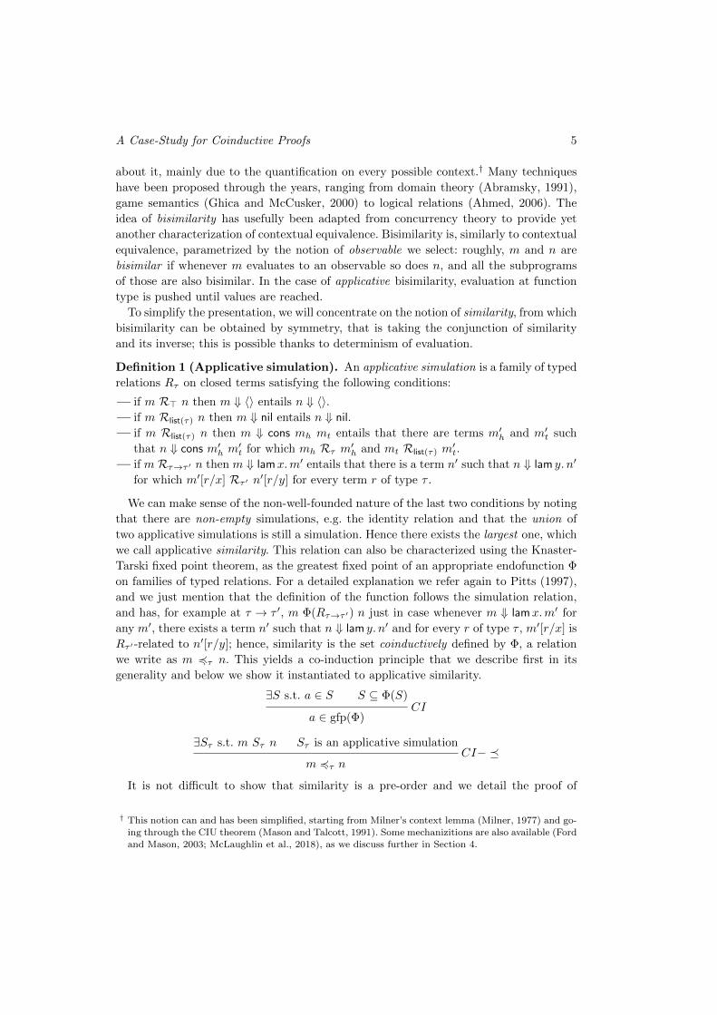
Definition 1 (Applicative simulation). An applicative simulation is a family of typed

relations Rτ on closed terms satisfying the following conditions:

— if m R> n then m ⇓ 〈〉 entails n ⇓ 〈〉.— if m Rlist(τ) n then m ⇓ nil entails n ⇓ nil.

— if m Rlist(τ) n then m ⇓ cons mh mt entails that there are terms m′h and m′t such

that n ⇓ cons m′h m′t for which mh Rτ m′h and mt Rlist(τ) m

′t.

— if m Rτ→τ ′ n then m ⇓ lamx.m′ entails that there is a term n′ such that n ⇓ lam y. n′

for which m′[r/x] Rτ ′ n′[r/y] for every term r of type τ .

We can make sense of the non-well-founded nature of the last two conditions by noting

that there are non-empty simulations, e.g. the identity relation and that the union of

two applicative simulations is still a simulation. Hence there exists the largest one, which

we call applicative similarity. This relation can also be characterized using the Knaster-

Tarski fixed point theorem, as the greatest fixed point of an appropriate endofunction Φ

on families of typed relations. For a detailed explanation we refer again to Pitts (1997),

and we just mention that the definition of the function follows the simulation relation,

and has, for example at τ → τ ′, m Φ(Rτ→τ ′) n just in case whenever m ⇓ lamx.m′ for

any m′, there exists a term n′ such that n ⇓ lam y. n′ and for every r of type τ , m′[r/x] is

Rτ ′ -related to n′[r/y]; hence, similarity is the set coinductively defined by Φ, a relation

we write as m 4τ n. This yields a co-induction principle that we describe first in its

generality and below we show it instantiated to applicative similarity.

∃S s.t. a ∈ S S ⊆ Φ(S)CI

a ∈ gfp(Φ)

∃Sτ s.t. m Sτ n Sτ is an applicative simulationCI− �

m 4τ n

It is not difficult to show that similarity is a pre-order and we detail the proof of

† This notion can and has been simplified, starting from Milner’s context lemma (Milner, 1977) and go-

ing through the CIU theorem (Mason and Talcott, 1991). Some mechanizitions are also available (Ford

and Mason, 2003; McLaughlin et al., 2018), as we discuss further in Section 4.

A. Momigliano, B. Pientka, and D. Thibodeau 6

reflexivity using rule CI− � to highlight the similarities with the type-theoretic definition

based instead on the notion of observation, on which our mechanization relies.

Theorem 1 (Reflexivity of applicative similarity). ∀m τ,m 4τ m.

Proof. To show the result we need to provide an appropriate simulation S and check

the simulation conditions. Just choose Sτ to be the family {(m,m) | · ` m : τ} where we

use the judgment m : τ to say that term m has type σ.

We then consider each case in the applicative simulation definition.

—if m S> m, then m ⇓ 〈〉 entails m ⇓ 〈〉: immediate;

—if m Slist(τ) m, then m ⇓ nil entails m ⇓ nil: immediate;

—assume m Slist(τ) m and m ⇓ cons mh mt; pick m′h,m′t to be mh,mt and by the

definition of the simulation, it holds that mh Sτ mh and mt Slist(τ) mt;

—assume m Sτ→τ ′ m and m ⇓ lamx.m′; again by picking m′ for n′ and by the definition

of the simulation it is obvious that for every r:τ , [r/x]m′ Sτ ′ [r/x]m′.

In many cases, we do not have to look much further beyond the statement of the

theorem to come up with an appropriate simulation, i.e. we can read off the definition

of simulation from it — and this is indeed the case for all the coinductive proofs in the

following development. However, to show the equivalence of specific programs we may

have to come up with a complex bisimulation, possibly defined inductively and/or “up

to”. This phenomenon is well-known in inductive theorem proving, where sometimes the

induction hypothesis coincides with the statement of the theorem, but in other cases it

needs to be generalized in an appropriate lemma. The fixed point rules conflate those two

aspects, generalization and lemma application, in one go. With an abuse of language, we

will say that we prove a statement by coinduction and say that we appeal to the use of

the “coinductive hypothesis” when the simulation corresponds to the statement of the

theorem.

When dealing with program equivalence, equational (in addition to coinductive) rea-

soning would be helpful and this is why it is crucial to establish bisimilarity to be a

congruence, i.e. a relation respecting the way terms are constructed. Since in this pa-

per we restrict ourselves to similarity, we target pre-congruence. Given the presence of

variable-binding operators, we need to consider relations over open terms, that is families

of relations over terms indexed by a typing context Γ in addition to a type τ , which we

write as Γ ` m Rτ n.

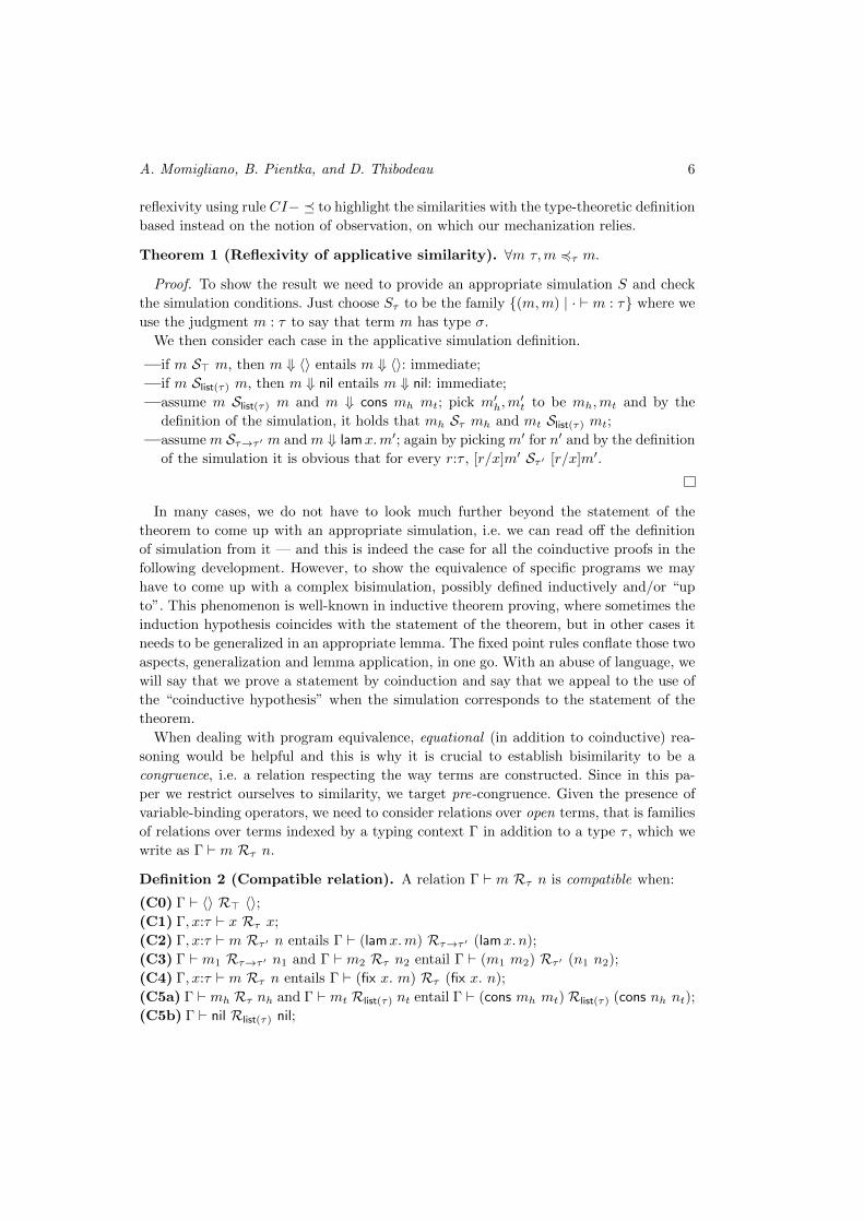
Definition 2 (Compatible relation). A relation Γ ` m Rτ n is compatible when:

(C0) Γ ` 〈〉 R> 〈〉;(C1) Γ, x:τ ` x Rτ x;

(C2) Γ, x:τ ` m Rτ ′ n entails Γ ` (lamx.m) Rτ→τ ′ (lamx. n);

(C3) Γ ` m1 Rτ→τ ′ n1 and Γ ` m2 Rτ n2 entail Γ ` (m1 m2) Rτ ′ (n1 n2);

(C4) Γ, x:τ ` m Rτ n entails Γ ` (fix x. m) Rτ (fix x. n);

(C5a) Γ ` mh Rτ nh and Γ ` mt Rlist(τ) nt entail Γ ` (cons mh mt)Rlist(τ) (cons nh nt);

(C5b) Γ ` nil Rlist(τ) nil;

A Case-Study for Coinductive Proofs 7

(C6) Γ ` m1 Rlist(τ) m2, Γ ` n1 Rτ ′ n2 and Γ, h:τ, t:list(τ) ` p1 Rτ ′ p2 entail Γ `(lcase m1 of {nil⇒ n1 | cons hd tl ⇒ p1})Rτ ′ (lcase m2 of {nil⇒ n2 | cons hd tl ⇒ p2}).

Definition 3 (Pre-congruence). A pre-congruence is a compatible transitive relation.

By the very definition of simulation at arrow type it is clear that a key property for

our development is for a relation to be preserved by pairwise substitution:

Γ, y:τ ` m1 Rτ ′ m2 and Γ ` n1 Rτ n2 entails Γ ` [n1/y]m1 Rτ ′ [n2/y]m2.

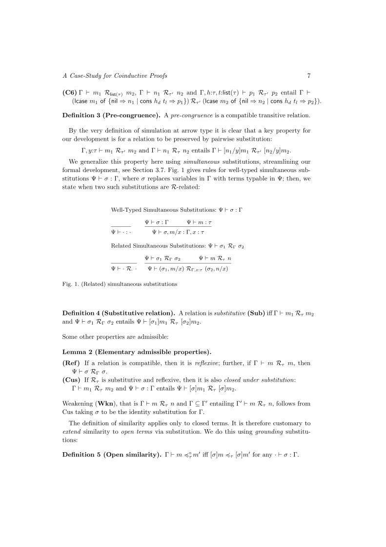
We generalize this property here using simultaneous substitutions, streamlining our

formal development, see Section 3.7. Fig. 1 gives rules for well-typed simultaneous sub-

stitutions Ψ ` σ : Γ, where σ replaces variables in Γ with terms typable in Ψ; then, we

state when two such substitutions are R-related:

Well-Typed Simultaneous Substitutions: Ψ ` σ : Γ

Ψ ` · : ·Ψ ` σ : Γ Ψ ` m : τ

Ψ ` σ,m/x : Γ, x : τ

Related Simultaneous Substitutions: Ψ ` σ1 RΓ σ2

Ψ ` · R· ·

Ψ ` σ1 RΓ σ2 Ψ ` m Rτ n

Ψ ` (σ1,m/x) RΓ,x:τ (σ2, n/x)

Fig. 1. (Related) simultaneous substitutions

Definition 4 (Substitutive relation). A relation is substitutive (Sub) iff Γ ` m1 Rτ m2

and Ψ ` σ1 RΓ σ2 entails Ψ ` [σ1]m1 Rτ [σ2]m2.

Some other properties are admissible:

Lemma 2 (Elementary admissible properties).

(Ref) If a relation is compatible, then it is reflexive; further, if Γ ` m Rτ m, then

Ψ ` σ RΓ σ.

(Cus) If Rτ is substitutive and reflexive, then it is also closed under substitution:

Γ ` m1 Rτ m2 and Ψ ` σ : Γ entails Ψ ` [σ]m1 Rτ [σ]m2.

Weakening (Wkn), that is Γ ` m Rτ n and Γ ⊆ Γ′ entailing Γ′ ` m Rτ n, follows from

Cus taking σ to be the identity substitution for Γ.

The definition of similarity applies only to closed terms. It is therefore customary to

extend similarity to open terms via substitution. We do this using grounding substitu-

tions:

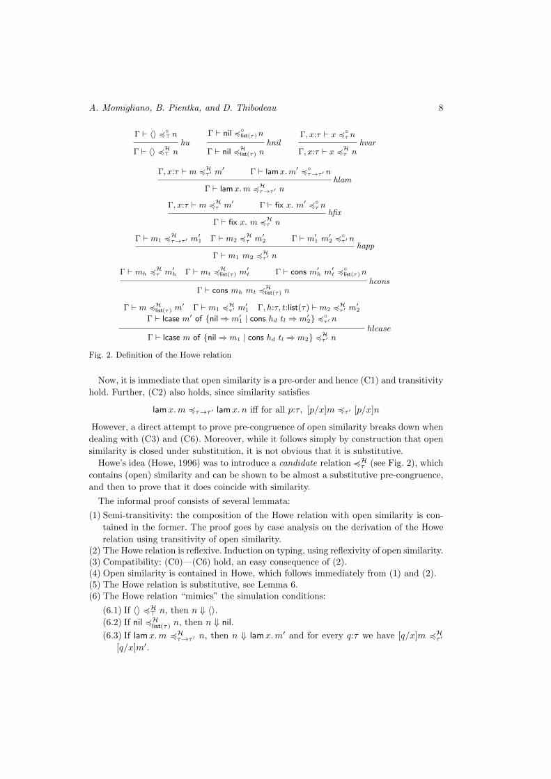
Definition 5 (Open similarity). Γ ` m 4◦τm′ iff [σ]m 4τ [σ]m′ for any · ` σ : Γ.

A. Momigliano, B. Pientka, and D. Thibodeau 8

Γ ` 〈〉 4◦>nhu

Γ ` 〈〉 4H> n

Γ ` nil 4◦list(τ)nhnil

Γ ` nil 4Hlist(τ) n

Γ, x:τ ` x 4◦τ nhvar

Γ, x:τ ` x 4Hτ n

Γ, x:τ ` m 4Hτ ′ m′ Γ ` lamx.m′ 4◦τ→τ ′ n

hlamΓ ` lamx.m 4Hτ→τ ′ n

Γ, x:τ ` m 4Hτ m′ Γ ` fix x. m′ 4◦τ nhfix

Γ ` fix x. m 4Hτ n

Γ ` m1 4Hτ→τ ′ m′1 Γ ` m2 4Hτ m′2 Γ ` m′1 m′2 4◦τ ′ n

happΓ ` m1 m2 4Hτ ′ n

Γ ` mh 4Hτ m′h Γ ` mt 4Hlist(τ) m

′t Γ ` cons m′h m

′t 4◦list(τ)n

hconsΓ ` cons mh mt 4

Hlist(τ) n

Γ ` m 4Hlist(τ) m′ Γ ` m1 4Hτ ′ m

′1 Γ, h:τ, t:list(τ) ` m2 4Hτ ′ m

′2

Γ ` lcase m′ of {nil⇒ m′1 | cons hd tl ⇒ m′2} 4◦τ ′ nhlcase

Γ ` lcase m of {nil⇒ m1 | cons hd tl ⇒ m2} 4Hτ ′ n

Fig. 2. Definition of the Howe relation

Now, it is immediate that open similarity is a pre-order and hence (C1) and transitivity

hold. Further, (C2) also holds, since similarity satisfies

lamx.m 4τ→τ ′ lamx. n iff for all p:τ, [p/x]m 4τ ′ [p/x]n

However, a direct attempt to prove pre-congruence of open similarity breaks down when

dealing with (C3) and (C6). Moreover, while it follows simply by construction that open

similarity is closed under substitution, it is not obvious that it is substitutive.

Howe’s idea (Howe, 1996) was to introduce a candidate relation 4Hτ (see Fig. 2), which

contains (open) similarity and can be shown to be almost a substitutive pre-congruence,

and then to prove that it does coincide with similarity.

The informal proof consists of several lemmata:

(1) Semi-transitivity: the composition of the Howe relation with open similarity is con-

tained in the former. The proof goes by case analysis on the derivation of the Howe

relation using transitivity of open similarity.(2) The Howe relation is reflexive. Induction on typing, using reflexivity of open similarity.(3) Compatibility: (C0)—(C6) hold, an easy consequence of (2).(4) Open similarity is contained in Howe, which follows immediately from (1) and (2).(5) The Howe relation is substitutive, see Lemma 6.(6) The Howe relation “mimics” the simulation conditions:

(6.1) If 〈〉 4H> n, then n ⇓ 〈〉.(6.2) If nil 4Hlist(τ) n, then n ⇓ nil.

(6.3) If lamx.m 4Hτ→τ ′ n, then n ⇓ lamx.m′ and for every q:τ we have [q/x]m 4Hτ ′

[q/x]m′.

A Case-Study for Coinductive Proofs 9

(6.4) If cons mh mt 4Hlist(τ) n, then n ⇓ cons ph pt, with mh 4Hτ ph and mt 4Hlist(τ) pt.

By inversion on the Howe relation and definition of similarity, using semi-transitivity

and, in the lambda-case, substitutivity of the Howe relation.

(7) Downward closure: if p 4Hτ q and p ⇓ v, then v 4Hτ q. Induction on evaluation, and

inversion on the Howe relation and similarity, with an additional case analysis on v.

(8) p 4Hτ q entails p 4τ q. By coinduction, using the coinductive hypothesis, point (6)

and (7).

Once all of these properties have been proved, we are ready for the main result, stating

that the Howe relation coincides with applicative similarity, and hence the pre-congruence

of the latter follows as a corollary:

Theorem 3. Γ ` p 4Hτ q iff Γ ` p 4◦τ q

Proof. Right to left is point (4) above. Conversely, proceed by induction on Γ using

(8) for the base case and closure under substitution for the step.

Corollary 1. Open similarity is a pre-congruence.

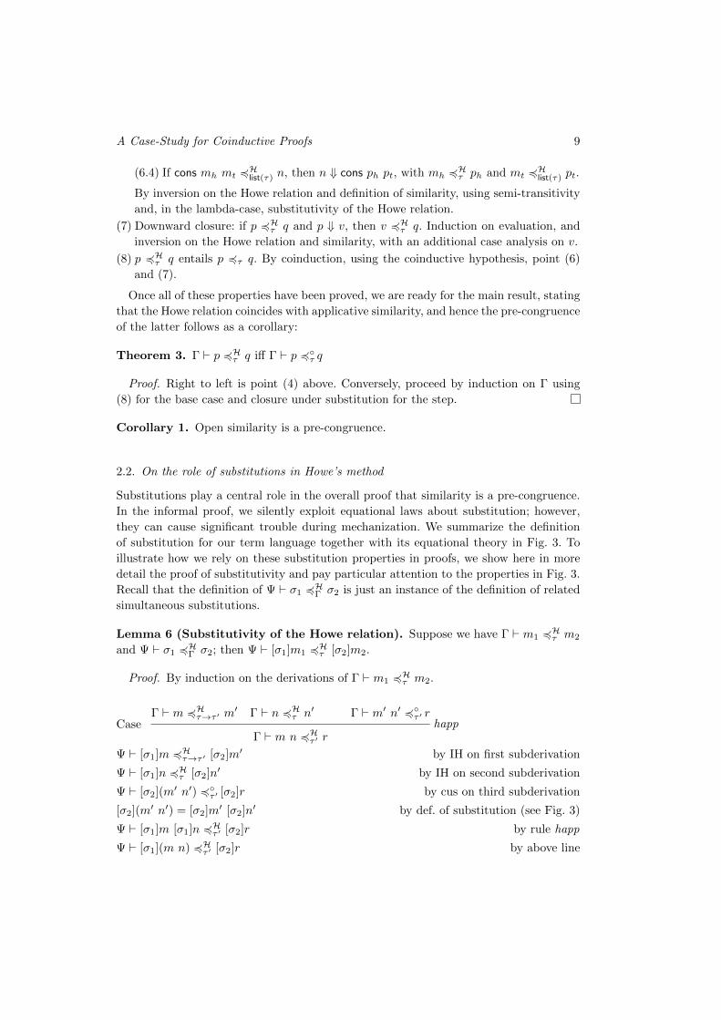
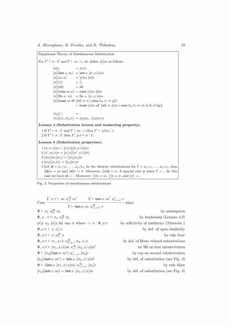
2.2. On the role of substitutions in Howe’s method

Substitutions play a central role in the overall proof that similarity is a pre-congruence.

In the informal proof, we silently exploit equational laws about substitution; however,

they can cause significant trouble during mechanization. We summarize the definition

of substitution for our term language together with its equational theory in Fig. 3. To

illustrate how we rely on these substitution properties in proofs, we show here in more

detail the proof of substitutivity and pay particular attention to the properties in Fig. 3.

Recall that the definition of Ψ ` σ1 4HΓ σ2 is just an instance of the definition of related

simultaneous substitutions.

Lemma 6 (Substitutivity of the Howe relation). Suppose we have Γ ` m1 4Hτ m2

and Ψ ` σ1 4HΓ σ2; then Ψ ` [σ1]m1 4Hτ [σ2]m2.

Proof. By induction on the derivations of Γ ` m1 4Hτ m2.

CaseΓ ` m 4Hτ→τ ′ m′ Γ ` n 4Hτ n′ Γ ` m′ n′ 4◦τ ′ r

happΓ ` m n 4Hτ ′ r

Ψ ` [σ1]m 4Hτ→τ ′ [σ2]m′ by IH on first subderivation

Ψ ` [σ1]n 4Hτ [σ2]n′ by IH on second subderivation

Ψ ` [σ2](m′ n′) 4◦τ ′ [σ2]r by cus on third subderivation

[σ2](m′ n′) = [σ2]m′ [σ2]n′ by def. of substitution (see Fig. 3)

Ψ ` [σ1]m [σ1]n 4Hτ ′ [σ2]r by rule happ

Ψ ` [σ1](m n) 4Hτ ′ [σ2]r by above line

A. Momigliano, B. Pientka, and D. Thibodeau 10

Equational Theory of Simultaneous Substitution

For Γ′ ` σ : Γ and Γ ` m : τ , we define [σ]m as follows

[σ]x = σ(x)

[σ](lamx.m) = lamx. [σ, x/x]m

[σ](m n) = [σ]m [σ]n

[σ](〈〉) = 〈〉[σ](nil) = nil

[σ](cons m n) = cons [σ]m [σ]n

[σ](fix x. m) = fix x. [σ, x/x]m

[σ](lcase m of {nil⇒ n | cons hd tl ⇒ p})= lcase [σ]m of {nil⇒ [σ]n | cons hd tl ⇒ [σ, h/h, t/t]p}

[σ2](·) = ·[σ2](σ1,m/x) = [σ2]σ1, [σ2]m/x

Lemma 4 (Substitution lemma and weakening property).

1 If Γ′ ` σ : Γ and Γ ` m : τ then Γ′ ` [σ]m : τ .

2 If Γ′ ` σ : Γ then Γ′, y:τ ` σ : Γ.

Lemma 5 (Substitution properties).

1 [σ, n/x]m = [n/x]([σ, x/x]m)

2 [σ′, n/x]σ = [n/x]([σ′, x/x]σ)

3 [σ2]([σ1]m1) = [[σ2]σ1]m

4 [σ2]([σ1]σ) = [[σ2]σ1]σ

5 Let id = x1/x1, . . . , xn/xn be the identity substitutions for Γ = x1:τ1, . . . , xn:τn, then

[id]m = m and [id]σ = σ. Moreover, [σ]id = σ. A special case is when Γ = ·. In this

case we have id = ·. Moreover, [·]m = m, [·]σ = σ, and [σ]· = ·.

Fig. 3. Properties of simultaneous substitutions

CaseΓ, x:τ ` m 4Hτ ′ m′ Γ ` lamx.m′ 4◦τ→τ ′ r

hlamΓ ` lamx.m 4Hτ→τ ′ r

Ψ ` σ1 4HΓ σ2 by assumption

Ψ, x : τ ` σ1 4HΓ σ2 by weakening (Lemma 4.2)

[σ]x 4τ [σ]x for any σ where · ` σ : Ψ, x:τ by reflexivity of similarity (Theorem 1

Ψ, x:τ ` x 4◦τ x by def. of open similarity

Ψ, x:τ ` x 4Hτ x by rule hvar

Ψ, x:τ ` σ1, x/x 4HΓ,x:τ σ2, x/x by def. of Howe related substitutions

Ψ, x:τ ` [σ1, x/x]m 4Hτ ′ [σ2, x/x]m′ by IH on first subderivation

Ψ ` [σ2](lamx.m′) 4◦τ→τ ′ [σ2]r by cus on second subderivation

[σ2](lamx.m′) = lamx. [σ2, x/x]m′ by def. of substitution (see Fig. 3)

Ψ ` (lamx. [σ1, x/x]m) 4Hτ→τ ′ [σ2]r by rule hlam

[σ1](lamx.m) = lamx. [σ1, x/x]m by def. of substitution (see Fig. 3)

A Case-Study for Coinductive Proofs 11

Ψ ` [σ1](lamx.m) 4Hτ→τ ′ [σ2]r by above line

The other cases are analogous.

3. Mechanizing Howe’s method in Beluga

We discuss in this Section the proof that similarity in PCFL is a pre-congruence using

Howe’s method in Beluga.

Beluga is a programming environment that supports both specifying formal systems

and reasoning about them. To specify formal systems such as PCFL we use the logical

framework LF. This allows us to take advantage of higher-order abstract syntax. A key

challenge when reasoning about LF objects is that we must consider potentially open

objects. In Beluga, this need is met by viewing all LF objects together with the contexts

in which they are meaningful (Nanevski et al., 2008) as contextual LF objects and by

abstracting not only over LF objects but also over contexts. We then view contextual

objects and contexts as a particular index domain about which we can reason using a

first-order logic with (co)induction principles on our index domain and built-in equality

on index objects. Under the Curry-Howard isomorphism this logic corresponds to a func-

tional language with indexed (co)inductive types that supports (co)pattern matching.

Meta-theoretic proofs about formal systems are implemented as (co)recursive functions

in Beluga. We summarize in Appendix A the source level syntax of Beluga, where we

concentrate on the parts that are relevant for our development. It is by no means a com-

plete description, but it may serve as a useful high-level introduction to understanding

Beluga programs. For a more formal introduction to the theoretical foundations, we refer

the reader to (Cave and Pientka, 2012; Thibodeau et al., 2016).

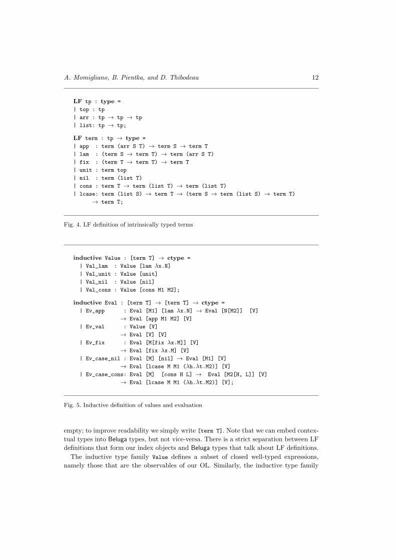
3.1. Encoding syntax in LF

We adopt the usual HOAS encoding for binding operators in the object language, and

make essential use of LF’s dependent types (see Fig. 4). In particular the type family

term encodes intrinsically-typed terms. This will make our overall mechanization more

compact, as all terms are well-typed by construction which is enforced by Beluga’s type

checker.

Variables such as T and S that are used in declaring the type of the LF constants

are abstracted over at the front of the type of the constructor and we rely on type

reconstruction to infer their types (Pientka, 2013). These variables are treated as implicit

and we subsequently omit passing them when forming term objects.

3.2. Encoding the operational semantics with indexed inductive types

To illustrate how we can use inductive types in Beluga, we encode the value and evaluation

judgment as computation-level type families indexed by closed well-typed terms. This is

demonstrably equivalent to encoding the same judgments at the LF level.

How do we enforce that a LF object is closed? This is accomplished by a contextual

type [ ` term T], where the context that appears to the left hand side of the turnstile is

A. Momigliano, B. Pientka, and D. Thibodeau 12

LF tp : type =

| top : tp

| arr : tp → tp → tp

| list: tp → tp;

LF term : tp → type =

| app : term (arr S T) → term S → term T

| lam : (term S → term T) → term (arr S T)

| fix : (term T → term T) → term T

| unit : term top

| nil : term (list T)

| cons : term T → term (list T) → term (list T)

| lcase: term (list S) → term T → (term S → term (list S) → term T)

→ term T;

Fig. 4. LF definition of intrinsically typed terms

inductive Value : [term T] → ctype =

| Val_lam : Value [lam λx.N]

| Val_unit : Value [unit]

| Val_nil : Value [nil]

| Val_cons : Value [cons M1 M2];

inductive Eval : [term T] → [term T] → ctype =

| Ev_app : Eval [M1] [lam λx.N] → Eval [N[M2]] [V]

→ Eval [app M1 M2] [V]

| Ev_val : Value [V]

→ Eval [V] [V]

| Ev_fix : Eval [M[fix λx.M]] [V]

→ Eval [fix λx.M] [V]

| Ev_case_nil : Eval [M] [nil] → Eval [M1] [V]

→ Eval [lcase M M1 (λh.λt.M2)] [V]

| Ev_case_cons: Eval [M] [cons H L] → Eval [M2[H, L]] [V]

→ Eval [lcase M M1 (λh.λt.M2)] [V];

Fig. 5. Inductive definition of values and evaluation

empty; to improve readability we simply write [term T]. Note that we can embed contex-

tual types into Beluga types, but not vice-versa. There is a strict separation between LF

definitions that form our index objects and Beluga types that talk about LF definitions.

The inductive type family Value defines a subset of closed well-typed expressions,

namely those that are the observables of our OL. Similarly, the inductive type family

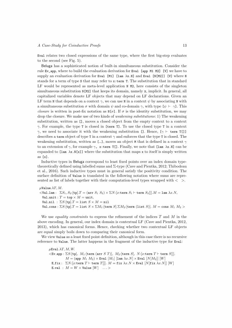
A Case-Study for Coinductive Proofs 13

Eval relates two closed expressions of the same type, where the first big-step evaluates

to the second (see Fig. 5).

Beluga has a sophisticated notion of built-in simultaneous substitution. Consider the

rule Ev_app, where to build the evaluation derivation for Eval [app M1 M2] [V] we have to

supply an evaluation derivation for Eval [M1] [lam λx.N] and Eval [N[M2]] [V] where N

stands for a term of type S that may refer to x:term T. The substitution that in standard

LF would be represented as meta-level application N M2, here consists of the singleton

simultaneous substitution N[M2] that keeps its domain, namely x, implicit. In general, all

capitalized variables denote LF objects that may depend on LF declarations. Given an

LF term N that depends on a context γ, we can use N in a context ψ by associating N with

a simultaneous substitution σ with domain ψ and co-domain γ, with type [ψ ` γ]. This

closure is written in post-fix notation as N[σ]. If σ is the identity substitution, we may

drop the closure. We make use of two kinds of weakening substitutions: 1) The weakening

substitution, written as [], moves a closed object from the empty context to a context

γ. For example, the type T is closed in [term T]. To use the closed type T in a context

γ, we need to associate it with the weakening substitution []. Hence, [γ ` term T[]]

describes a term object of type T in a context γ and enforces that the type T is closed. The

weakening substitution, written as [...], moves an object M that is defined in a context γ

to an extension of γ, for example γ, x:term T[]. Finally, we note that [lam λx.N] can be

expanded to [lam λx.N[x]] where the substitution that maps x to itself is simply written

as [x].

Inductive types in Beluga correspond to least fixed points over an index domain type-theoretically defined using labelled sums and Σ-type (Cave and Pientka, 2012; Thibodeauet al., 2016). Such inductive types must in general satisfy the positivity condition. Thesurface definition of Value is translated in the following notation where sums are repre-sented as list of labels together with their computation-level types wrapped with < >.

µValue.λT,M.

<Val lam : ΣS1, S2:[tp].T = (arr S1 S2)× ΣN :[x:term S1 ` term S2[]].M = lam λx.N,

Val unit : T = top×M = unit,

Val nil : ΣS:[tp].T = list S ×M = nil

Val cons : ΣS:[tp].T = list S × ΣM1:[term S].ΣM2:[term (list S)]. M = cons M1 M2 >

We use equality constraints to express the refinement of the indices T and M in the

above encoding. In general, our index domain is contextual LF (Cave and Pientka, 2012,

2013), which has canonical forms. Hence, checking whether two contextual LF objects

are equal simply boils down to comparing their canonical form.

We view Value as a least fixed point definition, although in this case there is no recursivereference to Value. The latter happens in the fragment of the inductive type for Eval:

µEval.λT,M,W.

<Ev app : ΣS:[tp], M1:[term (arr S T )], M2:[term S], N :[x:term T ` term S[]].

M = (app M1 M2)× Eval [M1] [lam λx.N ]× Eval [N [M2]] [W ]

E fix : ΣN :[x:term T ` term T []]. M = fix λx.N × Eval [N [fix λx.N ]] [W ]

E val : M = W × Value [W ] . . . >

A. Momigliano, B. Pientka, and D. Thibodeau 14

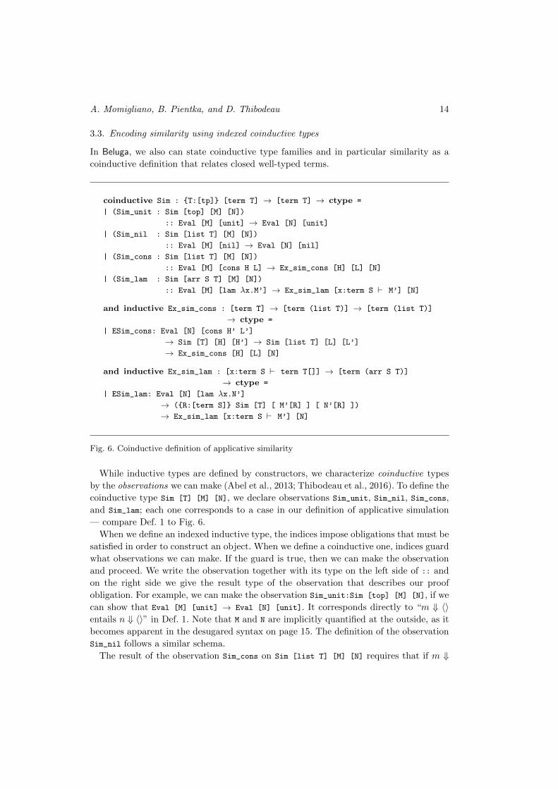
3.3. Encoding similarity using indexed coinductive types

In Beluga, we also can state coinductive type families and in particular similarity as a

coinductive definition that relates closed well-typed terms.

coinductive Sim : {T:[tp]} [term T] → [term T] → ctype =

| (Sim_unit : Sim [top] [M] [N])

:: Eval [M] [unit] → Eval [N] [unit]

| (Sim_nil : Sim [list T] [M] [N])

:: Eval [M] [nil] → Eval [N] [nil]

| (Sim_cons : Sim [list T] [M] [N])

:: Eval [M] [cons H L] → Ex_sim_cons [H] [L] [N]

| (Sim_lam : Sim [arr S T] [M] [N])

:: Eval [M] [lam λx.M’] → Ex_sim_lam [x:term S ` M’] [N]

and inductive Ex_sim_cons : [term T] → [term (list T)] → [term (list T)]

→ ctype =

| ESim_cons: Eval [N] [cons H’ L’]

→ Sim [T] [H] [H’] → Sim [list T] [L] [L’]

→ Ex_sim_cons [H] [L] [N]

and inductive Ex_sim_lam : [x:term S ` term T[]] → [term (arr S T)]

→ ctype =

| ESim_lam: Eval [N] [lam λx.N’]

→ ({R:[term S]} Sim [T] [ M’[R] ] [ N’[R] ])

→ Ex_sim_lam [x:term S ` M’] [N]

Fig. 6. Coinductive definition of applicative similarity

While inductive types are defined by constructors, we characterize coinductive types

by the observations we can make (Abel et al., 2013; Thibodeau et al., 2016). To define the

coinductive type Sim [T] [M] [N], we declare observations Sim_unit, Sim_nil, Sim_cons,

and Sim_lam; each one corresponds to a case in our definition of applicative simulation

— compare Def. 1 to Fig. 6.

When we define an indexed inductive type, the indices impose obligations that must be

satisfied in order to construct an object. When we define a coinductive one, indices guard

what observations we can make. If the guard is true, then we can make the observation

and proceed. We write the observation together with its type on the left side of :: and

on the right side we give the result type of the observation that describes our proof

obligation. For example, we can make the observation Sim_unit:Sim [top] [M] [N], if we

can show that Eval [M] [unit] → Eval [N] [unit]. It corresponds directly to “m ⇓ 〈〉entails n ⇓ 〈〉” in Def. 1. Note that M and N are implicitly quantified at the outside, as it

becomes apparent in the desugared syntax on page 15. The definition of the observation

Sim_nil follows a similar schema.

The result of the observation Sim_cons on Sim [list T] [M] [N] requires that if m ⇓

A Case-Study for Coinductive Proofs 15

cons h t then there are h′ and t′ such that n ⇓ cons h′ t′ for which h Rτ h′ and t Rlist(τ) t′.

We hence need a way to encode an existential property. Although existentials (i.e. Σ-

types) exist in our theoretical foundation, the implementation of Beluga does not support

them at the top level, as they always can be realized using indexed inductive types. We

therefore define an indexed inductive type Ex_sim_cons that relates h, t and n.

Last, we need to represent the result of observing Sim_lam that encodes the correspond-

ing part from the definition:

m ⇓ lamx.m′ for any x:τ ` m′:τ ′ entails that there exists a y:τ ` n′:τ ′ such that n ⇓ lam y. n′

for which m′[r/x] Rτ ′ n′[r/y] for every term r of type τ .

We again resort to defining an inductive type Ex_sim_lam that relates the term M’

with type [x:term S ` term T[]], i.e. M’ has type term T[] under the assumption of

the variable x having type term S. Hence we can simply write [x:term S ` M’], as we

interpret M’ within the context x:term S. As T denotes a closed type, we associate it with

a weakening substitution, since it is used in a non-empty context. The relation Ex_sim_lam

exists if Eval [N] [lam λx.N’] and for all R:[term S] we know Sim [T] [M’[R]] [N’[R]].

Finally, we remark that the coinductive type Sim and inductive types Ex_sim_cons and

Ex_sim_lam are defined mutually.

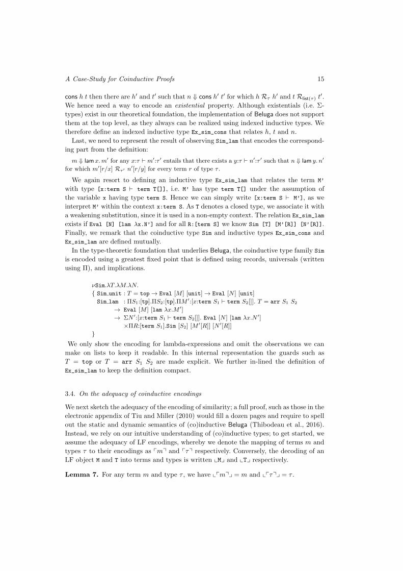
In the type-theoretic foundation that underlies Beluga, the coinductive type family Sim

is encoded using a greatest fixed point that is defined using records, universals (written

using Π), and implications.

νSim.λT.λM.λN.

{ Sim unit : T = top→ Eval [M ] [unit]→ Eval [N ] [unit]

Sim lam : ΠS1:[tp].ΠS2:[tp].ΠM ′:[x:term S1 ` term S2[]]. T = arr S1 S2

→ Eval [M ] [lam λx.M ′]

→ ΣN ′:[x:term S1 ` term S2[]]. Eval [N ] [lam λx.N ′]

×ΠR:[term S1].Sim [S2] [M ′[R]] [N ′[R]]

}We only show the encoding for lambda-expressions and omit the observations we can

make on lists to keep it readable. In this internal representation the guards such as

T = top or T = arr S1 S2 are made explicit. We further in-lined the definition of

Ex_sim_lam to keep the definition compact.

3.4. On the adequacy of coinductive encodings

We next sketch the adequacy of the encoding of similarity; a full proof, such as those in the

electronic appendix of Tiu and Miller (2010) would fill a dozen pages and require to spell

out the static and dynamic semantics of (co)inductive Beluga (Thibodeau et al., 2016).

Instead, we rely on our intuitive understanding of (co)inductive types; to get started, we

assume the adequacy of LF encodings, whereby we denote the mapping of terms m and

types τ to their encodings as pmq and pτq respectively. Conversely, the decoding of an

LF object M and T into terms and types is written xMy and xTy respectively.

Lemma 7. For any term m and type τ , we have xpmqy = m and xpτqy = τ .

A. Momigliano, B. Pientka, and D. Thibodeau 16

Proof. Standard, following for example Pfenning (1997).

We further build on the adequacy of the encoding of substitutions. In particular, the

translation of [σ]m is equivalent to first translating σ and the term m to their correspond-

ing representations in LF and then relying on the built-in simultaneous LF substitution

operation of applying pσq to pmq. The encoding pσq is defined inductively on the substi-

tution σ as expected: p·q =ˆand pσ,m/xq = pσq, pmq. Further, recall that we write the

application of a simultaneous LF substitution in prefix form, while we write the closure

of an LF object together with an LF substitution as a postfix.

Lemma 8 (Compositionality). p[σ]mq = [pσq]pmq.

Proof. Generalization of the compositionality lemma for LF.

Lemma 9 (Soundness). If Sim [pτq] [pmq] [pnq] then m 4τ n.

Proof. (Sketch) We apply rule CI− � to unfold m 4τ n selecting the family Sτ to be

{(m,n) | Sim [pτq] [pmq] [pnq]}

We then show that Sτ satisfies the simulation conditions unfolding the definition of Sτ .

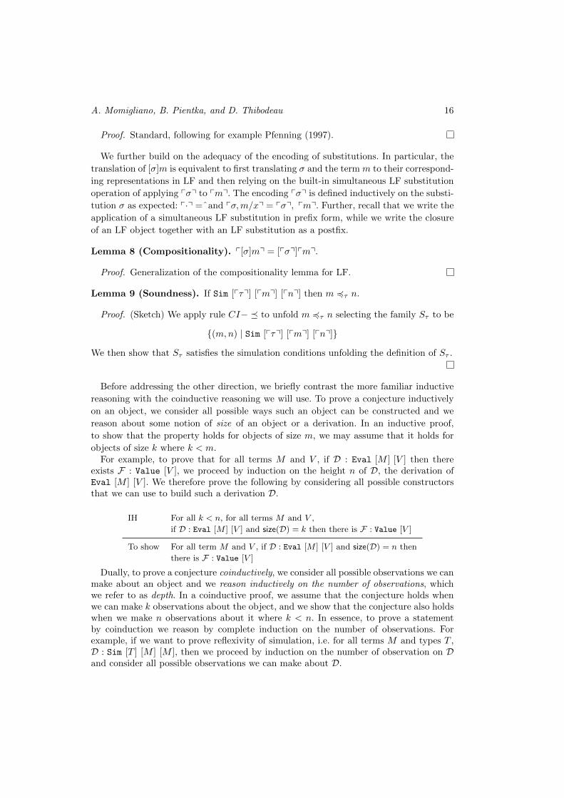
Before addressing the other direction, we briefly contrast the more familiar inductive

reasoning with the coinductive reasoning we will use. To prove a conjecture inductively

on an object, we consider all possible ways such an object can be constructed and we

reason about some notion of size of an object or a derivation. In an inductive proof,

to show that the property holds for objects of size m, we may assume that it holds for

objects of size k where k < m.For example, to prove that for all terms M and V , if D : Eval [M ] [V ] then there

exists F : Value [V ], we proceed by induction on the height n of D, the derivation ofEval [M ] [V ]. We therefore prove the following by considering all possible constructorsthat we can use to build such a derivation D.

IH For all k < n, for all terms M and V ,

if D : Eval [M ] [V ] and size(D) = k then there is F : Value [V ]

To show For all term M and V , if D : Eval [M ] [V ] and size(D) = n then

there is F : Value [V ]

Dually, to prove a conjecture coinductively, we consider all possible observations we canmake about an object and we reason inductively on the number of observations, whichwe refer to as depth. In a coinductive proof, we assume that the conjecture holds whenwe can make k observations about the object, and we show that the conjecture also holdswhen we make n observations about it where k < n. In essence, to prove a statementby coinduction we reason by complete induction on the number of observations. Forexample, if we want to prove reflexivity of simulation, i.e. for all terms M and types T ,D : Sim [T ] [M ] [M ], then we proceed by induction on the number of observation on Dand consider all possible observations we can make about D.

A Case-Study for Coinductive Proofs 17

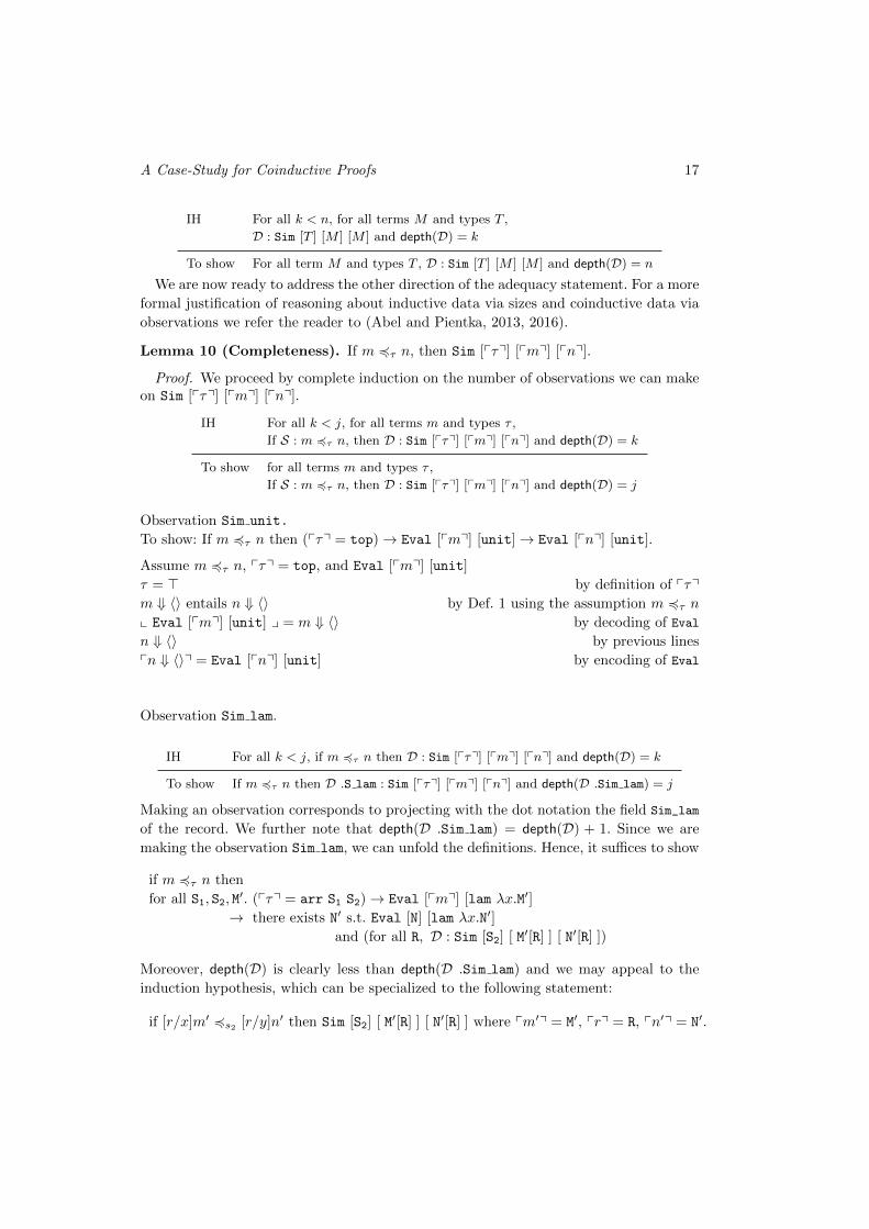
IH For all k < n, for all terms M and types T ,

D : Sim [T ] [M ] [M ] and depth(D) = k

To show For all term M and types T , D : Sim [T ] [M ] [M ] and depth(D) = n

We are now ready to address the other direction of the adequacy statement. For a more

formal justification of reasoning about inductive data via sizes and coinductive data via

observations we refer the reader to (Abel and Pientka, 2013, 2016).

Lemma 10 (Completeness). If m 4τ n, then Sim [pτq] [pmq] [pnq].

Proof. We proceed by complete induction on the number of observations we can makeon Sim [pτq] [pmq] [pnq].

IH For all k < j, for all terms m and types τ ,

If S : m 4τ n, then D : Sim [pτq] [pmq] [pnq] and depth(D) = k

To show for all terms m and types τ ,

If S : m 4τ n, then D : Sim [pτq] [pmq] [pnq] and depth(D) = j

Observation Sim unit.

To show: If m 4τ n then (pτq = top)→ Eval [pmq] [unit]→ Eval [pnq] [unit].

Assume m 4τ n, pτq = top, and Eval [pmq] [unit]

τ = > by definition of pτqm ⇓ 〈〉 entails n ⇓ 〈〉 by Def. 1 using the assumption m 4τ nx Eval [pmq] [unit] y = m ⇓ 〈〉 by decoding of Eval

n ⇓ 〈〉 by previous lines

pn ⇓ 〈〉q = Eval [pnq] [unit] by encoding of Eval

Observation Sim lam.

IH For all k < j, if m 4τ n then D : Sim [pτq] [pmq] [pnq] and depth(D) = k

To show If m 4τ n then D .S lam : Sim [pτq] [pmq] [pnq] and depth(D .Sim lam) = j

Making an observation corresponds to projecting with the dot notation the field Sim_lam

of the record. We further note that depth(D .Sim lam) = depth(D) + 1. Since we are

making the observation Sim lam, we can unfold the definitions. Hence, it suffices to show

if m 4τ n then

for all S1, S2, M′. (pτq = arr S1 S2)→ Eval [pmq] [lam λx.M′]

→ there exists N′ s.t. Eval [N] [lam λx.N′]

and (for all R, D : Sim [S2] [ M′[R] ] [ N′[R] ])

Moreover, depth(D) is clearly less than depth(D .Sim lam) and we may appeal to the

induction hypothesis, which can be specialized to the following statement:

if [r/x]m′ 4s2 [r/y]n′ then Sim [S2] [ M′[R] ] [ N′[R] ] where pm′q = M′, prq = R, pn′q = N′.

A. Momigliano, B. Pientka, and D. Thibodeau 18

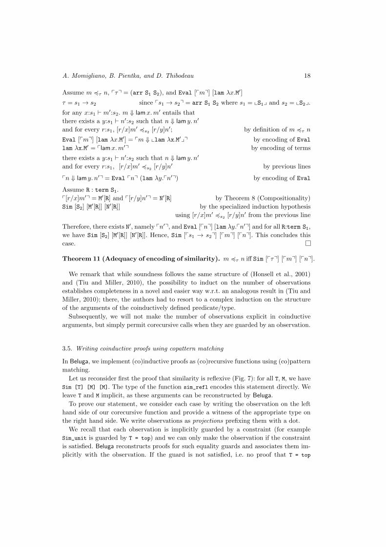
Assume m 4τ n, pτq = (arr S1 S2), and Eval [pmq] [lam λx.M′]

τ = s1 → s2 since ps1 → s2q = arr S1 S2 where s1 = xS1y and s2 = xS2y.

for any x:s1 ` m′:s2. m ⇓ lamx.m′ entails that

there exists a y:s1 ` n′:s2 such that n ⇓ lam y. n′

and for every r:s1, [r/x]m′ 4s2 [r/y]n′; by definition of m 4τ n

Eval [pmq] [lam λx.M′] = pm ⇓ xlam λx.M′yq by encoding of Eval

lam λx.M′ = plamx.m′q by encoding of terms

there exists a y:s1 ` n′:s2 such that n ⇓ lam y. n′

and for every r:s1, [r/x]m′ 4s2 [r/y]n′ by previous lines

pn ⇓ lam y. n′q = Eval pnq (lam λy.pn′q) by encoding of Eval

Assume R : term S1.

p[r/x]m′q = M′[R] and p[r/y]n′q = N′[R] by Theorem 8 (Compositionality)

Sim [S2] [M′[R]] [N′[R]] by the specialized induction hypothesis

using [r/x]m′ 4s2 [r/y]n′ from the previous line

Therefore, there exists N′, namely pn′q, and Eval [pnq] [lam λy.pn′q] and for all R:term S1,

we have Sim [S2] [M′[R]] [N′[R]]. Hence, Sim [ps1 → s2q] [pmq] [pnq]. This concludes this

case.

Theorem 11 (Adequacy of encoding of similarity). m 4τ n iff Sim [pτq] [pmq] [pnq].

We remark that while soundness follows the same structure of (Honsell et al., 2001)

and (Tiu and Miller, 2010), the possibility to induct on the number of observations

establishes completeness in a novel and easier way w.r.t. an analogous result in (Tiu and

Miller, 2010); there, the authors had to resort to a complex induction on the structure

of the arguments of the coinductively defined predicate/type.

Subsequently, we will not make the number of observations explicit in coinductive

arguments, but simply permit corecursive calls when they are guarded by an observation.

3.5. Writing coinductive proofs using copattern matching

In Beluga, we implement (co)inductive proofs as (co)recursive functions using (co)pattern

matching.

Let us reconsider first the proof that similarity is reflexive (Fig. 7): for all T, M, we have

Sim [T] [M] [M]. The type of the function sim_refl encodes this statement directly. We

leave T and M implicit, as these arguments can be reconstructed by Beluga.

To prove our statement, we consider each case by writing the observation on the left

hand side of our corecursive function and provide a witness of the appropriate type on

the right hand side. We write observations as projections prefixing them with a dot.

We recall that each observation is implicitly guarded by a constraint (for example

Sim_unit is guarded by T = top) and we can only make the observation if the constraint

is satisfied. Beluga reconstructs proofs for such equality guards and associates them im-

plicitly with the observation. If the guard is not satisfied, i.e. no proof that T = top

A Case-Study for Coinductive Proofs 19

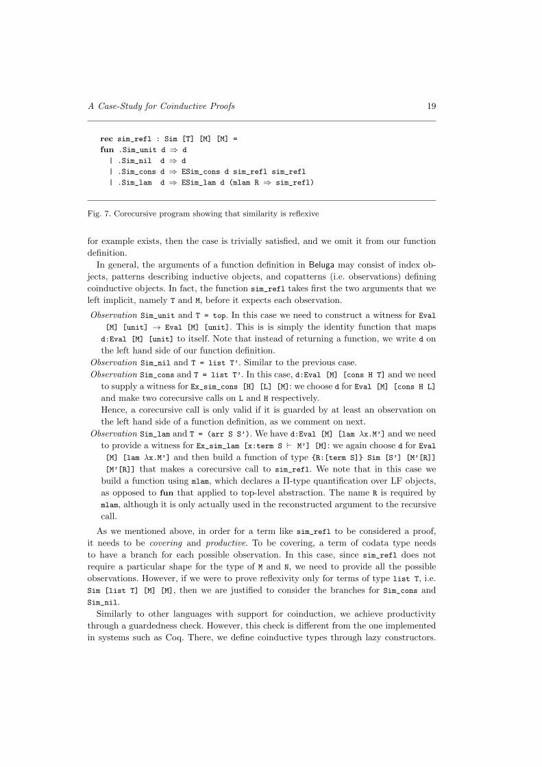
rec sim_refl : Sim [T] [M] [M] =

fun .Sim_unit d ⇒ d

| .Sim_nil d ⇒ d

| .Sim_cons d ⇒ ESim_cons d sim_refl sim_refl

| .Sim_lam d ⇒ ESim_lam d (mlam R ⇒ sim_refl)

Fig. 7. Corecursive program showing that similarity is reflexive

for example exists, then the case is trivially satisfied, and we omit it from our function

definition.

In general, the arguments of a function definition in Beluga may consist of index ob-

jects, patterns describing inductive objects, and copatterns (i.e. observations) defining

coinductive objects. In fact, the function sim_refl takes first the two arguments that we

left implicit, namely T and M, before it expects each observation.

Observation Sim_unit and T = top. In this case we need to construct a witness for Eval

[M] [unit] → Eval [M] [unit]. This is is simply the identity function that maps

d:Eval [M] [unit] to itself. Note that instead of returning a function, we write d on

the left hand side of our function definition.

Observation Sim_nil and T = list T’. Similar to the previous case.

Observation Sim_cons and T = list T’. In this case, d:Eval [M] [cons H T] and we need

to supply a witness for Ex_sim_cons [H] [L] [M]: we choose d for Eval [M] [cons H L]

and make two corecursive calls on L and H respectively.

Hence, a corecursive call is only valid if it is guarded by at least an observation on

the left hand side of a function definition, as we comment on next.

Observation Sim_lam and T = (arr S S’). We have d:Eval [M] [lam λx.M’] and we need

to provide a witness for Ex_sim_lam [x:term S ` M’] [M]: we again choose d for Eval

[M] [lam λx.M’] and then build a function of type {R:[term S]} Sim [S’] [M’[R]]

[M’[R]] that makes a corecursive call to sim_refl. We note that in this case we

build a function using mlam, which declares a Π-type quantification over LF objects,

as opposed to fun that applied to top-level abstraction. The name R is required by

mlam, although it is only actually used in the reconstructed argument to the recursive

call.

As we mentioned above, in order for a term like sim_refl to be considered a proof,

it needs to be covering and productive. To be covering, a term of codata type needs

to have a branch for each possible observation. In this case, since sim_refl does not

require a particular shape for the type of M and N, we need to provide all the possible

observations. However, if we were to prove reflexivity only for terms of type list T, i.e.

Sim [list T] [M] [M], then we are justified to consider the branches for Sim_cons and

Sim_nil.

Similarly to other languages with support for coinduction, we achieve productivity

through a guardedness check. However, this check is different from the one implemented

in systems such as Coq. There, we define coinductive types through lazy constructors.

A. Momigliano, B. Pientka, and D. Thibodeau 20

Thus, recursive calls are restricted, or guarded, as to be performed only under such con-

structors. With copatterns, coinductive terms are defined via observations that serve to

delay computation. As such, guardedness restricts recursive occurrences to be performed

under observations; hence each step of unfolding requires at least one observation to be

applied. For example, in the arrow case of the above proof, the corecursive call is justified,

as it is guarded by the observation .Sim_lam, which increases the number of observations

made. This is sufficient, as operationally each step of unfolding requires at least one

observation to be applied — otherwise the corecursive function could not progress.

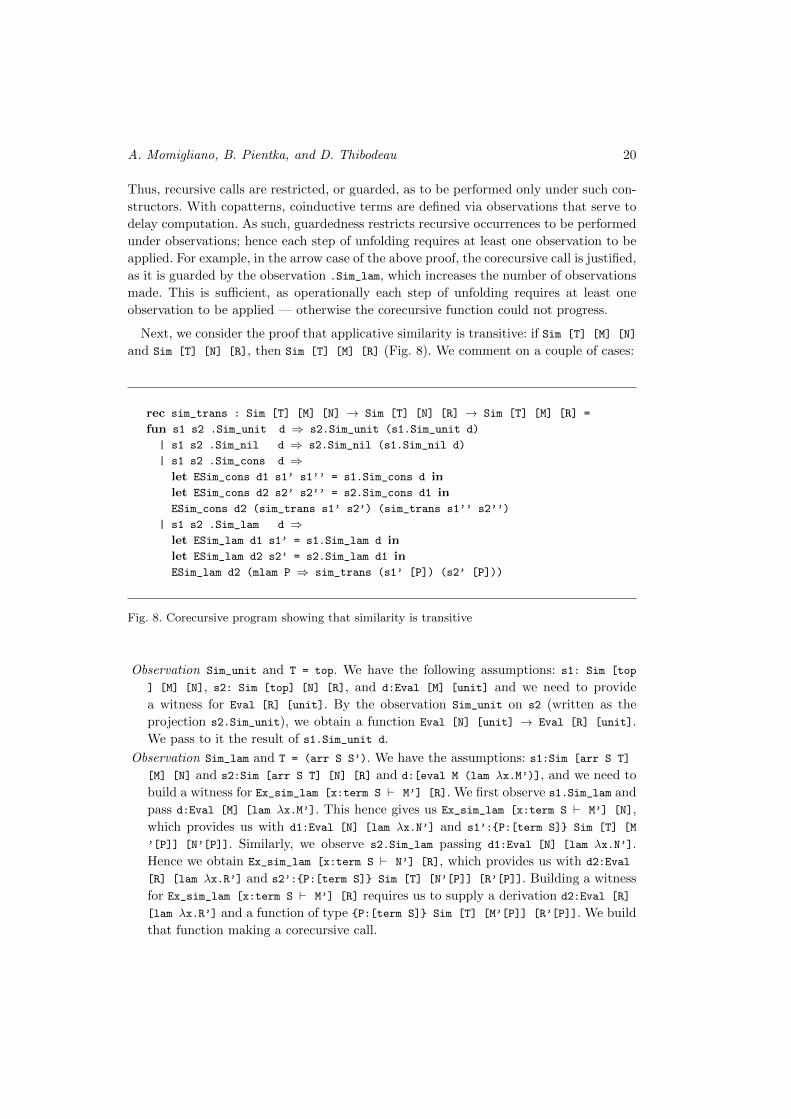
Next, we consider the proof that applicative similarity is transitive: if Sim [T] [M] [N]

and Sim [T] [N] [R], then Sim [T] [M] [R] (Fig. 8). We comment on a couple of cases:

rec sim_trans : Sim [T] [M] [N] → Sim [T] [N] [R] → Sim [T] [M] [R] =

fun s1 s2 .Sim_unit d ⇒ s2.Sim_unit (s1.Sim_unit d)

| s1 s2 .Sim_nil d ⇒ s2.Sim_nil (s1.Sim_nil d)

| s1 s2 .Sim_cons d ⇒let ESim_cons d1 s1’ s1’’ = s1.Sim_cons d in

let ESim_cons d2 s2’ s2’’ = s2.Sim_cons d1 in

ESim_cons d2 (sim_trans s1’ s2’) (sim_trans s1’’ s2’’)

| s1 s2 .Sim_lam d ⇒let ESim_lam d1 s1’ = s1.Sim_lam d in

let ESim_lam d2 s2’ = s2.Sim_lam d1 in

ESim_lam d2 (mlam P ⇒ sim_trans (s1’ [P]) (s2’ [P]))

Fig. 8. Corecursive program showing that similarity is transitive

Observation Sim_unit and T = top. We have the following assumptions: s1: Sim [top

] [M] [N], s2: Sim [top] [N] [R], and d:Eval [M] [unit] and we need to provide

a witness for Eval [R] [unit]. By the observation Sim_unit on s2 (written as the

projection s2.Sim_unit), we obtain a function Eval [N] [unit] → Eval [R] [unit].

We pass to it the result of s1.Sim_unit d.

Observation Sim_lam and T = (arr S S’). We have the assumptions: s1:Sim [arr S T]

[M] [N] and s2:Sim [arr S T] [N] [R] and d:[eval M (lam λx.M’)], and we need to

build a witness for Ex_sim_lam [x:term S ` M’] [R]. We first observe s1.Sim_lam and

pass d:Eval [M] [lam λx.M’]. This hence gives us Ex_sim_lam [x:term S ` M’] [N],

which provides us with d1:Eval [N] [lam λx.N’] and s1’:{P:[term S]} Sim [T] [M

’[P]] [N’[P]]. Similarly, we observe s2.Sim_lam passing d1:Eval [N] [lam λx.N’].

Hence we obtain Ex_sim_lam [x:term S ` N’] [R], which provides us with d2:Eval

[R] [lam λx.R’] and s2’:{P:[term S]} Sim [T] [N’[P]] [R’[P]]. Building a witness

for Ex_sim_lam [x:term S ` M’] [R] requires us to supply a derivation d2:Eval [R]

[lam λx.R’] and a function of type {P:[term S]} Sim [T] [M’[P]] [R’[P]]. We build

that function making a corecursive call.

A Case-Study for Coinductive Proofs 21

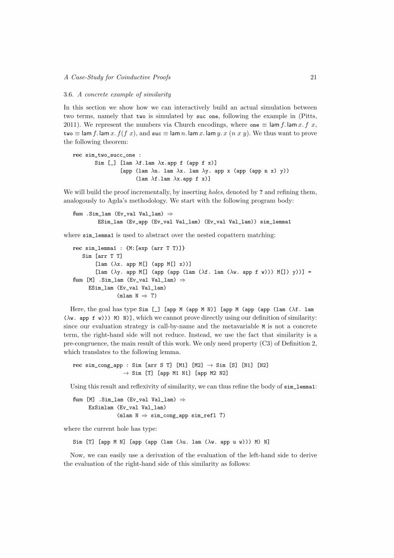
3.6. A concrete example of similarity

In this section we show how we can interactively build an actual simulation between

two terms, namely that two is simulated by suc one, following the example in (Pitts,

2011). We represent the numbers via Church encodings, where one ≡ lam f. lamx. f x,

two ≡ lam f. lamx. f(f x), and suc ≡ lamn. lamx. lam y. x (n x y). We thus want to prove

the following theorem:

rec sim_two_succ_one :

Sim [_] [lam λf.lam λx.app f (app f x)]

[app (lam λn. lam λx. lam λy. app x (app (app n x) y))

(lam λf.lam λx.app f x)]

We will build the proof incrementally, by inserting holes, denoted by ? and refining them,

analogously to Agda’s methodology. We start with the following program body:

fun .Sim_lam (Ev_val Val_lam) ⇒ESim_lam (Ev_app (Ev_val Val_lam) (Ev_val Val_lam)) sim_lemma1

where sim_lemma1 is used to abstract over the nested copattern matching:

rec sim_lemma1 : {M:[exp (arr T T)]}

Sim [arr T T]

[lam (λx. app M[] (app M[] x))]

[lam (λy. app M[] (app (app (lam (λf. lam (λw. app f w))) M[]) y))] =

fun [M] .Sim_lam (Ev_val Val_lam) ⇒ESim_lam (Ev_val Val_lam)

(mlam N ⇒ ?)

Here, the goal has type Sim [_] [app M (app M N)] [app M (app (app (lam (λf. lam

(λw. app f w))) M) N)], which we cannot prove directly using our definition of similarity:

since our evaluation strategy is call-by-name and the metavariable M is not a concrete

term, the right-hand side will not reduce. Instead, we use the fact that similarity is a

pre-congruence, the main result of this work. We only need property (C3) of Definition 2,

which translates to the following lemma.

rec sim_cong_app : Sim [arr S T] [M1] [M2] → Sim [S] [N1] [N2]

→ Sim [T] [app M1 N1] [app M2 N2]

Using this result and reflexivity of similarity, we can thus refine the body of sim_lemma1:

fun [M] .Sim_lam (Ev_val Val_lam) ⇒ExSimlam (Ev_val Val_lam)

(mlam N ⇒ sim_cong_app sim_refl ?)

where the current hole has type:

Sim [T] [app M N] [app (app (lam (λu. lam (λw. app u w))) M) N]

Now, we can easily use a derivation of the evaluation of the left-hand side to derive

the evaluation of the right-hand side of this similarity as follows:

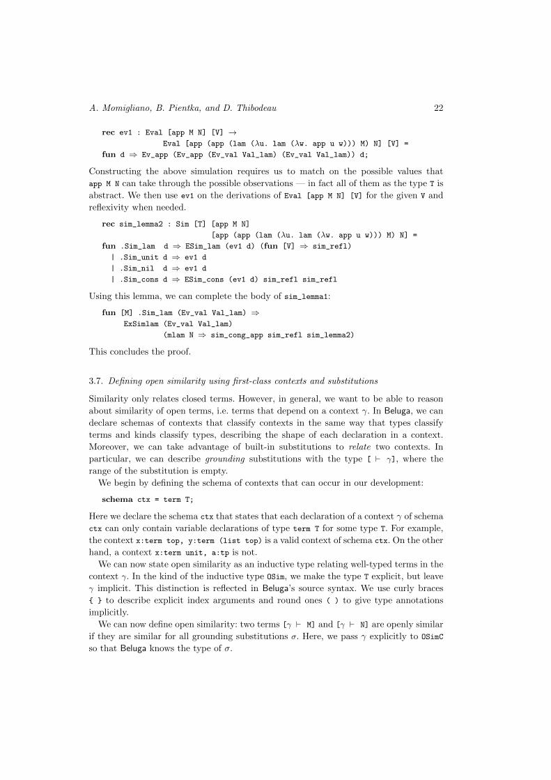
A. Momigliano, B. Pientka, and D. Thibodeau 22

rec ev1 : Eval [app M N] [V] →Eval [app (app (lam (λu. lam (λw. app u w))) M) N] [V] =

fun d ⇒ Ev_app (Ev_app (Ev_val Val_lam) (Ev_val Val_lam)) d;

Constructing the above simulation requires us to match on the possible values that

app M N can take through the possible observations — in fact all of them as the type T is

abstract. We then use ev1 on the derivations of Eval [app M N] [V] for the given V and

reflexivity when needed.

rec sim_lemma2 : Sim [T] [app M N]

[app (app (lam (λu. lam (λw. app u w))) M) N] =

fun .Sim_lam d ⇒ ESim_lam (ev1 d) (fun [V] ⇒ sim_refl)

| .Sim_unit d ⇒ ev1 d

| .Sim_nil d ⇒ ev1 d

| .Sim_cons d ⇒ ESim_cons (ev1 d) sim_refl sim_refl

Using this lemma, we can complete the body of sim_lemma1:

fun [M] .Sim_lam (Ev_val Val_lam) ⇒ExSimlam (Ev_val Val_lam)

(mlam N ⇒ sim_cong_app sim_refl sim_lemma2)

This concludes the proof.

3.7. Defining open similarity using first-class contexts and substitutions

Similarity only relates closed terms. However, in general, we want to be able to reason

about similarity of open terms, i.e. terms that depend on a context γ. In Beluga, we can

declare schemas of contexts that classify contexts in the same way that types classify

terms and kinds classify types, describing the shape of each declaration in a context.

Moreover, we can take advantage of built-in substitutions to relate two contexts. In

particular, we can describe grounding substitutions with the type [ ` γ], where the

range of the substitution is empty.

We begin by defining the schema of contexts that can occur in our development:

schema ctx = term T;

Here we declare the schema ctx that states that each declaration of a context γ of schema

ctx can only contain variable declarations of type term T for some type T. For example,

the context x:term top, y:term (list top) is a valid context of schema ctx. On the other

hand, a context x:term unit, a:tp is not.

We can now state open similarity as an inductive type relating well-typed terms in the

context γ. In the kind of the inductive type OSim, we make the type T explicit, but leave

γ implicit. This distinction is reflected in Beluga’s source syntax. We use curly braces

{ } to describe explicit index arguments and round ones ( ) to give type annotations

implicitly.

We can now define open similarity: two terms [γ ` M] and [γ ` N] are openly similar

if they are similar for all grounding substitutions σ. Here, we pass γ explicitly to OSimC

so that Beluga knows the type of σ.

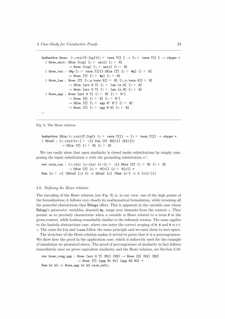
A Case-Study for Coinductive Proofs 23

inductive Howe: (γ:ctx){T:[tp]}[γ ` term T[] ] → [γ ` term T[] ] → ctype =

| Howe_unit: OSim [top] [γ ` unit] [γ ` M]

→ Howe [top] [γ ` unit] [γ ` M]

| Howe_var : {#p:[γ ` term T[]]} OSim [T] [γ ` #p] [γ ` M]

→ Howe [T] [γ ` #p] [γ ` M]

| Howe_lam : Howe [T] [γ,x:term S[] ` M] [γ,x:term S[] ` N]

→ OSim [arr S T] [γ ` lam λx.N] [γ ` R]

→ Howe [arr S T] [γ ` lam λx.M] [γ ` R]

| Howe_app : Howe [arr S T] [γ ` M] [γ ` M’]

→ Howe [S] [γ ` N] [γ ` N’]

→ OSim [T] [γ ` app M’ N’] [γ ` R]

→ Howe [T] [γ ` app M N] [γ ` R]

...

Fig. 9. The Howe relation

inductive OSim:(γ:ctx){T:[tp]} [γ ` term T[]] → [γ ` term T[]] → ctype =

| OSimC : {γ:ctx}({σ:[ ` γ]} Sim [T] [M[σ]] [N[σ]])

→ OSim [T] [γ ` M] [γ ` N]

We can easily show that open similarity is closed under substitutions by simply com-

posing the input substitution σ with the grounding substitution σ’.

rec osim_cus : (γ:ctx) (ψ:ctx) {σ:[ψ ` γ]} OSim [T] [γ ` M] [γ ` N]

→ OSim [T] [ψ ` M[σ]] [ψ ` N[σ]] =

fun [ψ ` σ] (OSimC [γ] f) ⇒ OSimC [ψ] (fun [σ’] ⇒ f [σ[σ’]])

3.8. Defining the Howe relation

The encoding of the Howe relation (see Fig. 9) is, in our view, one of the high points of

the formalization: it follows very closely its mathematical formulation, while retaining all

the powerful abstractions that Beluga offers. This is apparent in the variable case where

Beluga’s parameter variables, denoted #p, range over elements from the context γ. They

permit us to precisely characterize when a variable is Howe related to a term M in the

given context, while looking remarkably similar to the informal version. The same applies

to the lambda abstractions case, where one notes the correct scoping of M, N and R w.r.t.

γ. The cases for fix and lcase follow the same principle and we omit them to save space.

The structure of the Howe relation makes it trivial to prove that it is a precongruence.

We show here the proof in the application case, which is indirectly used for the example

of simulation we presented above. The proof of precongruence of similarity in fact follows

immediately once we prove equivalent similarity and the Howe relation, see Section 3.10.

rec howe_cong_app : Howe [arr S T] [M1] [M2] → Howe [S] [N1] [N2]

→ Howe [T] [app M1 N1] [app M2 N2] =

fun h1 h2 ⇒ Howe_app h1 h2 osim_refl;

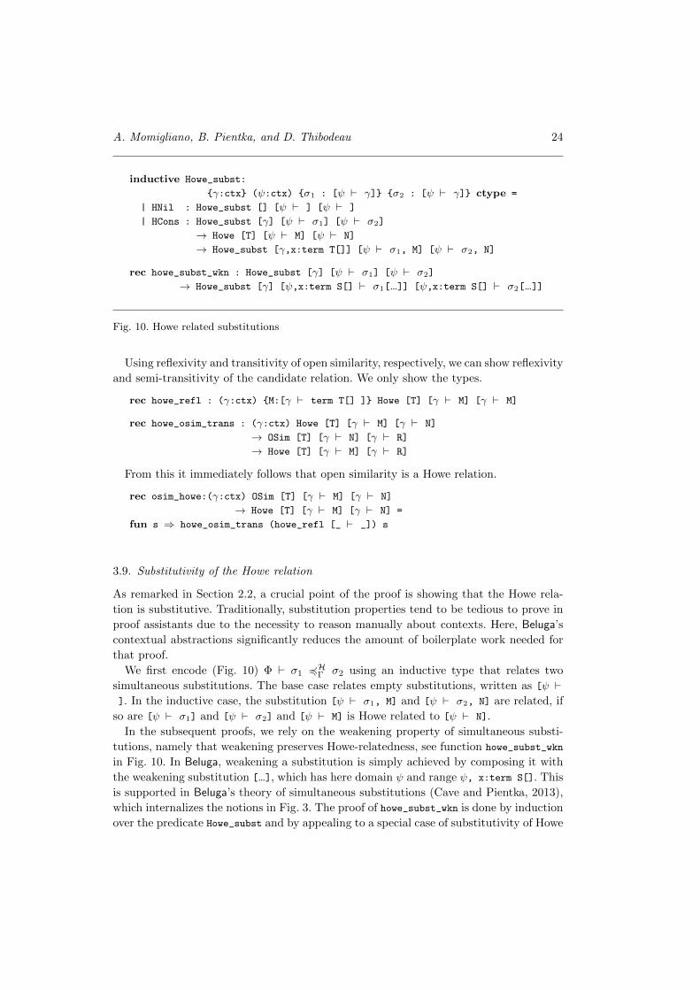
A. Momigliano, B. Pientka, and D. Thibodeau 24

inductive Howe_subst:

{γ:ctx} (ψ:ctx) {σ1 : [ψ ` γ]} {σ2 : [ψ ` γ]} ctype =

| HNil : Howe_subst [] [ψ ` ] [ψ ` ]

| HCons : Howe_subst [γ] [ψ ` σ1] [ψ ` σ2]

→ Howe [T] [ψ ` M] [ψ ` N]

→ Howe_subst [γ,x:term T[]] [ψ ` σ1, M] [ψ ` σ2, N]

rec howe_subst_wkn : Howe_subst [γ] [ψ ` σ1] [ψ ` σ2]

→ Howe_subst [γ] [ψ,x:term S[] ` σ1[...]] [ψ,x:term S[] ` σ2[...]]

Fig. 10. Howe related substitutions

Using reflexivity and transitivity of open similarity, respectively, we can show reflexivity

and semi-transitivity of the candidate relation. We only show the types.

rec howe_refl : (γ:ctx) {M:[γ ` term T[] ]} Howe [T] [γ ` M] [γ ` M]

rec howe_osim_trans : (γ:ctx) Howe [T] [γ ` M] [γ ` N]

→ OSim [T] [γ ` N] [γ ` R]

→ Howe [T] [γ ` M] [γ ` R]

From this it immediately follows that open similarity is a Howe relation.

rec osim_howe:(γ:ctx) OSim [T] [γ ` M] [γ ` N]

→ Howe [T] [γ ` M] [γ ` N] =

fun s ⇒ howe_osim_trans (howe_refl [_ ` _]) s

3.9. Substitutivity of the Howe relation

As remarked in Section 2.2, a crucial point of the proof is showing that the Howe rela-

tion is substitutive. Traditionally, substitution properties tend to be tedious to prove in

proof assistants due to the necessity to reason manually about contexts. Here, Beluga’s

contextual abstractions significantly reduces the amount of boilerplate work needed for

that proof.

We first encode (Fig. 10) Φ ` σ1 4HΓ σ2 using an inductive type that relates two

simultaneous substitutions. The base case relates empty substitutions, written as [ψ `]. In the inductive case, the substitution [ψ ` σ1, M] and [ψ ` σ2, N] are related, if

so are [ψ ` σ1] and [ψ ` σ2] and [ψ ` M] is Howe related to [ψ ` N].

In the subsequent proofs, we rely on the weakening property of simultaneous substi-

tutions, namely that weakening preserves Howe-relatedness, see function howe_subst_wkn

in Fig. 10. In Beluga, weakening a substitution is simply achieved by composing it with

the weakening substitution [...], which has here domain ψ and range ψ, x:term S[]. This

is supported in Beluga’s theory of simultaneous substitutions (Cave and Pientka, 2013),

which internalizes the notions in Fig. 3. The proof of howe_subst_wkn is done by induction

over the predicate Howe_subst and by appealing to a special case of substitutivity of Howe

A Case-Study for Coinductive Proofs 25

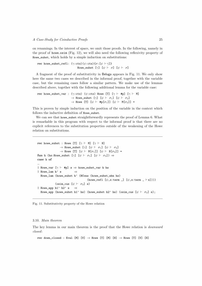
on renamings. In the interest of space, we omit those proofs. In the following, namely in

the proof of howe osim (Fig. 12), we will also need the following reflexivity property of

Howe_subst, which holds by a simple induction on substitutions:

rec howe_subst_refl: (γ:ctx)(ψ:ctx){σ:[ψ ` γ]}Howe_subst [γ] [ψ ` σ] [ψ ` σ]

A fragment of the proof of substitutivity in Beluga appears in Fig. 11. We only show

here the same two cases we described in the informal proof, together with the variable

case, but the remaining cases follow a similar pattern. We make use of the lemmas

described above, together with the following additional lemma for the variable case:

rec howe_subst_var : (γ:ctx) (ψ:ctx) Howe [T] [γ ` #p] [γ ` M]

→ Howe_subst [γ] [ψ ` σ1] [ψ ` σ2]

→ Howe [T] [ψ ` #p[σ1]] [ψ ` M[σ2]] =

This is proven by simple induction on the position of the variable in the context which

follows the inductive definition of Howe_subst.

We can see that howe_subst straightforwardly represents the proof of Lemma 6. What

is remarkable in this program with respect to the informal proof is that there are no

explicit references to the substitution properties outside of the weakening of the Howe

relation on substitutions.

rec howe_subst : Howe [T] [γ ` M] [γ ` N]

→ Howe_subst [γ] [ψ ` σ1] [ψ ` σ2]

→ Howe [T] [ψ ` M[σ1]] [ψ ` N[σ2]] =

fun h (hs:Howe_subst [γ] [ψ ` σ1] [ψ ` σ2]) ⇒case h of

...

| Howe_var [γ ` #p] s ⇒ howe_subst_var h hs

| Howe_lam h’ s ⇒Howe_lam (howe_subst h’ (HCons (howe_subst_wkn hs)

(howe_refl [ψ,x:term _] [ψ,x:term _ ` x])))(osim_cus [ψ ` σ2] s)

| Howe_app h1’ h2’ s ⇒Howe_app (howe_subst h1’ hs) (howe_subst h2’ hs) (osim_cus [ψ ` σ2] s);

Fig. 11. Substitutivity property of the Howe relation

3.10. Main theorem

The key lemma in our main theorem is the proof that the Howe relation is downward

closed :

rec down_closed : Eval [M] [V] → Howe [T] [M] [N] → Howe [T] [V] [N]

A. Momigliano, B. Pientka, and D. Thibodeau 26

rec howe_sim : Howe [T] [M] [N] → Sim [T] [M] [N] =

fun h .Sim_unit e ⇒ howe_ev_unit (down_closed e h)

| h .Sim_nil e ⇒ howe_ev_nil (down_closed e h)

| h .Sim_cons e ⇒let Howe_consC e’ h1 h2 = howe_ev_cons (down_closed e h) in

ESim_cons e’ (howe_sim h1) (howe_sim h2)

| h .Sim_lam e ⇒let Howe_absC e’ f = howe_ev_abs (down_closed e h) in

ESim_lam e’ (mlam R ⇒ howe_sim (f [R])

rec howe_osim : {γ:ctx} Howe [T] [γ ` M] [γ ` N]

→ OSim [T] [γ ` M] [γ ` N] =

fun [γ] h ⇒ OSimC (mlam σ ⇒ howe_sim (howe_subst h (howeSubst_refl [σ])));

Fig. 12. The Howe relation is included in open similarity

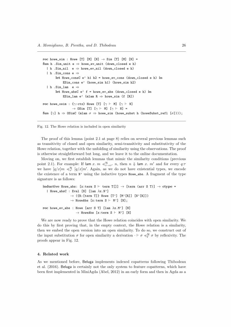
The proof of this lemma (point 2.1 at page 8) relies on several previous lemmas such

as transitivity of closed and open similarity, semi-transitivity and substitutivity of the

Howe relation, together with the unfolding of similarity using the observations. The proof

is otherwise straightforward but long, and we leave it to the online documentation.

Moving on, we first establish lemmas that mimic the similarity conditions (previous

point 2.1). For example: If lam x. m 4Hτ→τ ′ n, then n ⇓ lam x. m′ and for every q:τ

we have [q/x]m 4Hτ ′ [q/x]m′. Again, as we do not have existential types, we encode

the existence of a term N’ using the inductive types Howe_abs. A fragment of the type

signature is as follows:

inductive Howe_abs: [x:term S ` term T[]] → [term (arr S T)] → ctype =

| Howe_absC : Eval [N] [lam λx.N’]

→ ({R:[term T]} Howe [T’] [M’[R]] [N’[R]])

→ HoweAbs [x:term S ` M’] [N];

rec howe_ev_abs : Howe [arr S T] [lam λx.M’] [N]

→ HoweAbs [x:term S ` M’] [N]

We are now ready to prove that the Howe relation coincides with open similarity. We

do this by first proving that, in the empty context, the Howe relation is a similarity,

then we embed the open version into an open similarity. To do so, we construct out of

the input substitution σ for open similarity a derivation · ` σ 4HΓ σ by reflexivity. The

proofs appear in Fig. 12.

4. Related work

As we mentioned before, Beluga implements indexed copatterns following Thibodeau

et al. (2016). Beluga is certainly not the only system to feature copatterns, which have

been first implemented in MiniAgda (Abel, 2012) in an early form and then in Agda as a

A Case-Study for Coinductive Proofs 27

prototype (Abel et al., 2013). Copatterns now show up even in mainstream programming

languages such as OCaml (Laforgue and Regis-Gianas, 2017) as they allow us to integrate

elegantly lazy evaluation within an eager language. However, Beluga is the only system

supporting coinductive reasoning about HOAS representation using copatterns.

The observation paradigm differs from a more traditional approach using lazy con-

structors as adopted by Coq (Gimenez, 1996), in that coinductive types are defined by

their elimination rules as opposed to their introduction rules. Coq’s intensional type the-

ory offers a strong decidable equational theory through dependent pattern matching, but

loses subject reduction in the presence of coinduction (Oury, 2008). In fact, the change

of paradigm to observations was proposed to overcome that very issue with subject re-

duction when mixing lazy constructors with dependent case analysis (Abel et al., 2013).

Isabelle recently also overhauled (see for example (Biendarra et al., 2017)) their handling

of coinduction.

The first HOAS-like formal verification of the congruence of a notion of bisimilarity

concerned the π-calculus (Honsell et al., 2001) and was carried out in Coq using the Weak

HOAS approach and instantiating the Theory of Contexts to axiomatizing properties of

names. As common in many coinductive developments in Coq, the authors soon ran afoul

of the guardedness checker in Cofix-style proofs and had to resort to an explicit greatest-

fixed point encoding for Strong Late Bisimilairy. Abella’s take on the same issue (Tiu

and Miller, 2010) seems preferable; that paper details, among so much more, a proof that

similarity is a pre-congruence for the finite π-calculus. The encoding is rather elegant,

where all issues involving bindings, names, and substitutions are handled declaratively

without explicit side-conditions, thanks to the ∇-quantifier. This style of encoding has

been extended in (Chaudhuri et al., 2015) to handle bisimilarity “up-to”. This is achieved

via a limited form of quantification on relations that does not have, to our knowledge,

a consistency proof yet. The authors do not pursue a proof of congruence in the cited

paper.

Recent years have seen much work regarding the formalization of process calculi, in

particular using Nominal Isabelle. We do not have the space to discuss this line of work

in detail but simply cite some of the many contributions from Parrow and his asso-

ciates (Bengtson and Parrow, 2009; Parrow et al., 2014; Bengtson et al., 2016) about

various versions of the π/ψ-calculus and their congruence properties, proven without

resorting to the Howe’s proof strategy.

Encoding bisimilarity in the λ-calculus, in particular via Howe’s method, brings in

additional challenges, as we have seen. We are aware of several formalizations through

the years:

1. In (Ambler and Crole, 1999) the authors verify in Isabelle/HOL 98 the same result

of the present paper and a bit more (they also show that similarity coincides with

contextual pre-order) for PCFL using de Bruijn indexes as an encoding techniques

for binders. The development, for the congruence part, consists of around 160 lem-

mas/theorems, and it confirms a common belief about (standard) concrete syntax

approaches: doable, but very hard-going;

2. A partial improvement was presented in (Momigliano et al., 2002), which was based

A. Momigliano, B. Pientka, and D. Thibodeau 28

on the HOAS approach implemented in an early version of the Hybrid tool (Felty

and Momigliano, 2012), but one crucial lemma was left unproven, tellingly: Howe’s

substitutivity. This was related to the difficulty of lifting substitution as β-conversion

to substitution on judgments in one-level Hybrid term;3. In Momigliano (2012) the author fixed this problem, giving a complete Abella proof

for the simply typed calculus with unit. The proof consists of circa 45 theorems, 1/4

of which devoted to maintaining typing invariants in (open) similarity and in the

candidate relation, 1/7 of which instead used to make sure that some ∇-quantified

variable cannot occur in certain predicates. The main source of difficulty was again in

the proof of substitutivity of the Howe relation, in particular while handling structural

properties of explicit contexts.4. Using the present paper as a blue print, Chaudhuri (2018) gives a proof in Abella

of the substitutivity of the Howe relation that is very close to the one discussed

here; it is based on a theory of first class simultaneous substitutions encoded via

the copy clauses as originally suggested by Miller: m1/x1, . . . ,mn/xn is represented

as the Abella context copy xn Mn :: ... :: copy x1 M1 :: nil. The application

of a substitution [σ]m = n becomes the derivability of the judgment {pσq ` copy

pmq pnq}. The theory underlying this formalization consists of 15 theorems, 4 of

which are sensitive to the signature: in this sense the theory has to be stated and re-

proven for each signature. Compared to the Beluga development, where substitutions

and their equality theory are built-in, this is more labour-intense roughly adding a

factor of 1.6. Moreover, Abella’s proposed handling of simultaneous substitutions is,

of course, relational and must be explicitly applied whenever needed. For example,

the proof of osim ocus, which in Beluga is a one liner, requires here the appeal to

five lemmas to ensure that substitutions and their compositions are functional, that

types and well-formedness of contexts are preserved etc.

In another recent paper McLaughlin et al. (2018) give a formalization of the coincidence

of observational and applicative approximation not going through the candidate relation,

but triangulating with a notion of logical (as in logical relations) approximation. This

is then extended to CIU approximation. The encoding uses first-order syntax for terms,

but a form of weak HOAS for judgments following Allais et al. (2017), and it is therefore

compatible with a standard proof assistant such as Agda. Similarly to us, it leverages

the use of intrinsically well-typed and well-scoped terms and simultaneous substitutions,

although the latter are not supported natively by the framework. Interestingly, it offers

an elegant notion of concrete context (and thus of Morris approximation) that seems

much easier to reason with than previous efforts (Ford and Mason, 2003).

Lenglet and Schmitt (2018) present a formalization of Sangiorgi’s Higher-Order π-

calculus in Coq, using the locally nameless approach to representing name restriction and

well-scoped de Bruijn indices for process variables. The formalization includes a proof

that strong context bisimilarity is a congruence, via an adaptation to the concurrent

setting of Howe’s method. The authors seem unaware of HOAS representations of the

π-calculus and the representation technique adopted, albeit state of the art among the

concrete ones, still requires a lot of boilerplate infrastructure to handle names and related

notions.

A Case-Study for Coinductive Proofs 29

5. Conclusions and future work

We have outlined how to use Beluga to encode a significant example of reasoning about

program equivalence using Howe’s method for PCFL. This has reinforced several obser-

vations that we have been making in other case studies, viz. (Cave and Pientka, 2015,

2018):

— Using intrinsically typed terms instead of working with explicit typing invariants

makes our encoding more compact and easier to deal with, since HOAS maintains

our terms well-scoped. The advantages of intrinsically typed representations have also

been observed in non-HOAS setting (Benton et al., 2012; Allais et al., 2017).

— The support for built-in simultaneous substitutions and contexts lead us to generalize

some statements, for example substitutivity; this paid off in our mechanization, as

many crucial lemmas became simpler to prove.

— Thanks to catering for both indexed inductive and coinductive data-types in Beluga,

the encoding of similarity and of the candidate relation was concise and as close as

the informal presentation as one can reasonably hope for.

An important question, when discussing formalizations, regards trust in mechanized

proofs. There are two aspects that play a role: the first concerns the theoretical founda-

tions underlying a proof environment and the second the implementation of that foun-

dation in a concrete system. Beluga’s theoretical foundation provides the justification

for reading its programs as proofs. For reasoning inductively directly over contextual

LF objects, we exploit the subterm ordering on LF terms, see (Pientka, 2005; Pientka

and Abel, 2015). Our (co)inductive programs give a high-level surface language to the

core calculus described in Jacob-Rao et al. (2018). Coverage for our programs using

(co)pattern matching is described in Thibodeau et al. (2016) and the well-foundedness

of such programs is justified by reasoning about sizes, where the size describes the depth

of observations in the co-recursive case (Abel and Pientka, 2016, 2013). Hence, the theo-

retical foundations for justifying the formalization of this case study are well developed.

However, the implementation of these theoretical ideas in Beluga (status: July 2018) —

as it is often the case — lags slightly behind; in particular, we are in the process of

extending the implementation of our totality checker to support simultaneous copattern

matching Thibodeau et al. (2016); Abel and Pientka (2013). This would allow us not

only to certify inductive proofs, but also coinductive ones.

While we hope that we have convinced the reader that Beluga is an excellent envi-

ronment for the meta-theory of program equivalence, this case study has shown that is

not well suited (yet) to verifying the equivalence of concrete pieces of code. To approach

this, we need not only to improve the interactive proof construction mode similarly to

what Agda offers, but to investigate proof search (Baelde et al., 2007) and model check-

ing (Cheney and Momigliano, 2017).

Last but not least, let us take a look beyond mechanizing bisimilarity that has been

the focus of this paper: the attentive reader may have noticed that we have not proven

that bisimilarity coincides with contextual equivalence, as e.g., in (Ambler and Crole,

1999). The challenge lies in the encoding of the latter notion: we would rather avoid

A. Momigliano, B. Pientka, and D. Thibodeau 30

using a notion of concrete non-α-equivalent terms with holes, in favour of a context-

less formulation, whereby contextual equivalence can be seen as the largest adequate and

compatible relation (Lassen, 1998; Pitts, 2011). This requires extending Beluga to at least

second-order quantification. This is work in progress, as it would be useful in many other

scenarios, e g., normalization for system F .

Finally, we believe it would be interesting to explore other approaches to proving pro-

gram equivalence such as step-indexed logical relations (Ahmed, 2006) and compare this

approach with Howe’s. This would give us a deeper understanding of program equivalence

proofs and provide insights into how both approaches scale to more complex program-

ming languages such as in (Pitts, 2005; Crary and Harper, 2007).

References

Abel, A. (2012). Type-based termination, inflationary fixed-points, and mixed inductive-

coinductive types. In Invited Talk at 8th Workshop on Fixed-points in Computer Sci-

ence (FICS’12), pages 1–11.

Abel, A. and Pientka, B. (2013). Well-founded recursion with copatterns:a unified ap-

proach to termination and productivity. In Proceedings of the 18th International Con-

ference on Functional Programming (ICFP ’13), pages 185–196.

Abel, A. and Pientka, B. (2016). Well-founded recursion with copatterns and sized types.

Journal of Functional Programming, 26:e2 (61 pages).

Abel, A., Pientka, B., Thibodeau, D., and Setzer, A. (2013). Copatterns: Programming

infinite structures by observations. In 40th Symp. on Principles of Programming Lan-

guages (POPL’13), pages 27–38. ACM Press.

Abramsky, S. (1991). A domain equation for bisimulation. Inf. Comput., 92(2):161–218.

Ahmed, A. (2006). Step-indexed syntactic logical relations for recursive and quantified

types. In Sestoft, P., editor, 15th European Symposium on Programming (ESOP’06),

pages 69–83. Springer.

Allais, G., Chapman, J., McBride, C., and McKinna, J. (2017). Type-and-scope safe

programs and their proofs. In Bertot, Y. and Vafeiadis, V., editors, 6th Conference on

Certified Programs and Proofs (CPP’17), pages 195–207. ACM.

Ambler, S. and Crole, R. L. (1999). Mechanized operational semantics via (co)induction.

In Bertot, Y., Dowek, G., Hirschowitz, A., Paulin, C., and Thery, L., editors, 12th

International Conference on Theorem Proving in Higher Order Logics (TPHOLs’99),

Lecture Notes in Computer Science (LNCS 1690), pages 221–238. Springer.

Baelde, D., Chaudhuri, K., Gacek, A., Miller, D., Nadathur, G., Tiu, A., and Wang,

Y. (2014). Abella: A system for reasoning about relational specifications. Journal of

Formalized Reasoning, 7(2):1–89.

Baelde, D., Gacek, A., Miller, D., Nadathur, G., and Tiu, A. (2007). The Bedwyr sys-

tem for model checking over syntactic expressions. In 21st Conference on Automated

Deduction (CADE), Lecture Notes in Computer Science (LNCS 4603), pages 391–397.

Springer.

Bengtson, J. and Parrow, J. (2009). Formalising the pi-calculus using nominal logic.

Logical Methods in Computer Science, 5(2).

A Case-Study for Coinductive Proofs 31

Bengtson, J., Parrow, J., and Weber, T. (2016). Psi-calculi in Isabelle. J. Autom.

Reasoning, 56(1):1–47.

Benton, N., Hur, C., Kennedy, A., and McBride, C. (2012). Strongly typed term repre-

sentations in coq. J. Autom. Reasoning, 49(2):141–159.

Biendarra, J., Blanchette, J. C., Bouzy, A., Desharnais, M., Fleury, M., Holzl, J., Kuncar,

O., Lochbihler, A., Meier, F., Panny, L., Popescu, A., Sternagel, C., Thiemann, R.,

and Traytel, D. (2017). Foundational (co)datatypes and (co)recursion for higher-order

logic. In Dixon, C. and Finger, M., editors, 11th International Symposium on Frontiers

of Combining Systems (FroCoS’17), Lecture Notes in Computer Science (LNCS 10483),

pages 3–21. Springer.

Cave, A. and Pientka, B. (2012). Programming with binders and indexed data-types. In

39th Symposium on Principles of Programming Languages (POPL’12), pages 413–424.

ACM Press.

Cave, A. and Pientka, B. (2013). First-class substitutions in contextual type theory. In 8th

ACM SIGPLAN International Workshop on Logical Frameworks and Meta-Languages:

Theory and Practice (LFMTP’13), pages 15–24. ACM Press.

Cave, A. and Pientka, B. (2015). A case study on logical relations using contextual

types. In Cervesato, I. and Chaudhuri, K., editors, 10th International Workshop on

Logical Frameworks and Meta-Languages: Theory and Practice (LFMTP’15), pages

18–33. Electronic Proceedings in Theoretical Computer Science (EPTCS).

Cave, A. and Pientka, B. (2018). Mechanizing Proofs with Logical Relations – Kripke-

style. Mathematical Structures in Computer Science, pages 1 – 33. Published online

August 2018.

Chaudhuri, K. (2018). A two-level logic perspective on (simultaneous) substitutions.

In Andronick, J. and Felty, A. P., editors, Proceedings of the 7th ACM SIGPLAN

International Conference on Certified Programs and Proofs, CPP 2018, Los Angeles,

CA, USA, January 8-9, 2018, pages 280–292. ACM.

Chaudhuri, K., Cimini, M., and Miller, D. (2015). A lightweight formalization of the

metatheory of bisimulation-up-to. In Leroy, X. and Tiu, A., editors, Proceedings of

the 2015 Conference on Certified Programs and Proofs, CPP 2015, Mumbai, India,

January 15-17, 2015, pages 157–166. ACM.

Cheney, J. and Momigliano, A. (2017). αcheck: A mechanized metatheory model checker.

TPLP, 17(3):311–352.

Crary, K. and Harper, R. (2007). Syntactic logical relations for polymorphic and recursive

types. Electr. Notes Theor. Comput. Sci., 172:259–299.

Felty, A. P. and Momigliano, A. (2012). Hybrid: A definitional two-level approach to rea-

soning with higher-order abstract syntax. Journal of Automated Reasoning, 48(1):43–

105.

Ford, J. and Mason, I. A. (2003). Formal foundations of operational semantics. Higher-

Order and Symbolic Computation, 16(3):161–202.

Ghica, D. R. and McCusker, G. (2000). Reasoning about idealized ALGOL using regular

languages. In Montanari, U., Rolim, J. D. P., and Welzl, E., editors, Automata, Lan-

guages and Programming, 27th International Colloquium, ICALP 2000, Proceedings,

volume 1853 of Lecture Notes in Computer Science, pages 103–115. Springer.

A. Momigliano, B. Pientka, and D. Thibodeau 32

Gimenez, E. (1996). Un Calcul de Constructions Infinies et son application a la

verification de systemes communicants. PhD thesis, Ecole Normale Superieure de

Lyon. These d’universite.Harper, R., Honsell, F., and Plotkin, G. (1993). A framework for defining logics. Journal

of the ACM, 40(1):143–184.Hirschkoff, D. (1997). A full formalisation of pi-calculus theory in the calculus of con-

structions. In Gunter, E. L. and Felty, A. P., editors, 10th International Conference on

Theorem Proving in Higher Order Logics (TPHOLs’97), Lecture Notes in Computer

Science (LNCS 1275), pages 153–169. Springer.Honsell, F., Miculan, M., and Scagnetto, I. (2001). Π-calculus in (co)inductive type

theories. Theoretical Computer Science, 2(253):239–285.Howe, D. J. (1996). Proving congruence of bisimulation in functional programming

languages. Information and Computation, 124(2):103–112.Jacob-Rao, R., Pientka, B., and Thibodeau, D. (2018). Index-stratified types. In Kirch-

ner, H., editor, 3rdd International Conference on Formal Structures for Computa-

tion and Deduction (FSCD’18), LIPIcs, pages 19:1–19:17. Schloss Dagstuhl - Leibniz-

Zentrum fur Informatik.Laforgue, P. and Regis-Gianas, Y. (2017). Copattern matching and first-class observa-

tions in OCaml, with a macro. In Proceedings of the 19th International Symposium on

Principles and Practice of Declarative Programming, PPDP ’17, pages 97–108.Lassen, S. B. (1998). Relational Reasoning about Functions and Nondeterminism. PhD

thesis, Dept of Computer Science, Univ of Aarhus.Lee, D. K., Crary, K., and Harper, R. (2007). Towards a mechanized metatheory of Stan-

dard ML. In 34th Symposium on Principles of Programming Languages (POPL’07),

pages 173–184. ACM Press.Lenglet, S. and Schmitt, A. (2018). Hoπ in coq. In Andronick, J. and Felty, A. P.,

editors, Proceedings of the 7th ACM SIGPLAN International Conference on Certified

Programs and Proofs, CPP 2018, Los Angeles, CA, USA, January 8-9, 2018, pages

252–265. ACM.Mason, I. and Talcott, C. (1991). Equivalence in functional languages with effects. Jour-

nal of Functional Programming, 1(03):287–327.McDowell, R. and Miller, D. (1997). A logic for reasoning with higher-order abstract

syntax. In Winskel, G., editor, 12th Symp. on Logic in Computer Science, pages 434–

445. IEEE Computer Society Press.McDowell, R., Miller, D., and Palamidessi, C. (1996). Encoding transition systems in

sequent calculus: Preliminary report. Electronic Notes in Theoretical Computer Science

(ENTCS), 3.McLaughlin, C., McKinna, J., and Stark, I. (2018). Triangulating context lemmas. In

Andronick, J. and Felty, A. P., editors, Proceedings of the 7th ACM SIGPLAN Inter-

national Conference on Certified Programs and Proofs, CPP 2018, Los Angeles, CA,

USA, January 8-9, 2018, pages 102–114. ACM.Miller, D. and Nadathur, G. (2012). Programming with Higher-Order Logic. Cambridge

University Press, New York, NY, USA, 1st edition.Miller, D. and Palamidessi, C. (1999). Foundational aspects of syntax. ACM Comput.

Surv., 31(3es).

A Case-Study for Coinductive Proofs 33

Miller, D. and Tiu, A. (2005). A proof theory for generic judgments. ACM Trans.

Comput. Log., 6(4):749–783.

Milner, R. (1977). Fully abstract models of typed -calculi. Theoretical Computer Science,

4(1):1 – 22.

Momigliano, A. (2012). A supposedly fun thing I may have to do again: A HOAS

encoding of Howe’s method. In 7nth International Workshop on Logical Frameworks

and Meta-languages: Theory and Practice (LFMTP’12), pages 33–42. ACM.

Momigliano, A., Ambler, S., and Crole, R. L. (2002). A Hybrid encoding of Howe’s

method for establishing congruence of bisimilarity. Electr. Notes Theor. Comput. Sci.,

70(2).

Momigliano, A. and Tiu, A. (2003). Induction and co-induction in sequent calculus. In

Coppo, M., Berardi, S., and Damiani, F., editors, Post-proceedings of TYPES 2003,

Lecture Notes in Computer Science (LNCS 3085), pages 293–308.

Nanevski, A., Pfenning, F., and Pientka, B. (2008). Contextual modal type theory. ACM

Transactions on Computational Logic, 9(3):1–49.

Oury, N. (2008). Coinductive types and type preservation. Message on the coq-club

mailing list.

Parrow, J., Borgstrom, J., Raabjerg, P., and Pohjola, J. A. (2014). Higher-order psi-

calculi. Mathematical Structures in Computer Science, 24(2).

Pfenning, F. (1997). Computation and deduction. Accessed January 31st, 2018.

Pfenning, F. and Schurmann, C. (1999). System description: Twelf — a meta-logical

framework for deductive systems. In Ganzinger, H., editor, 16th International Con-

ference on Automated Deduction (CADE-16), Lecture Notes in Artificial Intelligence

(LNAI 1632), pages 202–206. Springer.

Pientka, B. (2005). Verifying termination and reduction properties about higher-order

logic programs. Journal of Automated Reasoning, 34(2):179–207.

Pientka, B. (2008). A type-theoretic foundation for programming with higher-order

abstract syntax and first-class substitutions. In 35th Symposium on Principles of

Programming Languages (POPL’08), pages 371–382. ACM Press.

Pientka, B. (2013). An insider’s look at LF type reconstruction: Everything you never

wanted to know. J. Funct. Program., 23(1):1–37.

Pientka, B. and Abel, A. (2015). Structural recursion over contextual objects. In Al-

tenkirch, T., editor, 13th International Conference on Typed Lambda Calculi and Ap-

plications (TLCA’15), pages 273–287. Leibniz International Proceedings in Informatics

(LIPIcs) of Schloss Dagstuhl.

Pientka, B. and Cave, A. (2015). Inductive Beluga: Programming Proofs (System De-

scription). In Felty, A. P. and Middeldorp, A., editors, 25th International Conference on

Automated Deduction (CADE-25), Lecture Notes in Computer Science (LNCS 9195),

pages 272–281. Springer.

Pientka, B. and Dunfield, J. (2008). Programming with proofs and explicit contexts. In

Antoy, S. and Albert, E., editors, Proceedings of the 10th International ACM SIGPLAN

Conference on Principles and Practice of Declarative Programming, July 15-17, 2008,

Valencia, Spain, pages 163–173. ACM.

Pientka, B. and Dunfield, J. (2010). Beluga: a framework for programming and reasoning

A. Momigliano, B. Pientka, and D. Thibodeau 34

with deductive systems (System Description). In Giesl, J. and Haehnle, R., editors, 5th

International Joint Conference on Automated Reasoning (IJCAR’10), Lecture Notes

in Artificial Intelligence (LNAI 6173), pages 15–21. Springer.

Pitts, A. M. (1997). Operationally Based Theories of Program Equivalence. In Dybjer,

P. and Pitts, A. M., editors, Semantics and Logics of Computation.

Pitts, A. M. (2005). Typed operational reasoning. In Pierce, B. C., editor, Advanced

Topics in Types and Programming Languages, chapter 7, pages 245–289. The MIT

Press.

Pitts, A. M. (2011). Howe’s method for higher-order languages. In Sangiorgi, D. and

Rutten, J., editors, Advanced Topics in Bisimulation and Coinduction, volume 52 of

Cambridge Tracts in Theoretical Computer Science, chapter 5, pages 197–232. Cam-

bridge University Press.

Thibodeau, D., Cave, A., and Pientka, B. (2016). Indexed codata. In Garrigue, J., Keller,

G., and Sumii, E., editors, 21st International Conference on Functional Programming

(ICFP’16), pages 351–363. ACM.

Tiu, A. and Miller, D. (2010). Proof search specifications of bisimulation and modal

logics for the π-calculus. ACM Trans. Comput. Logic, 11(2):1–35.

Tiu, A. and Momigliano, A. (2012). Cut elimination for a logic with induction and

co-induction. J. Applied Logic, 10(4):330–367.

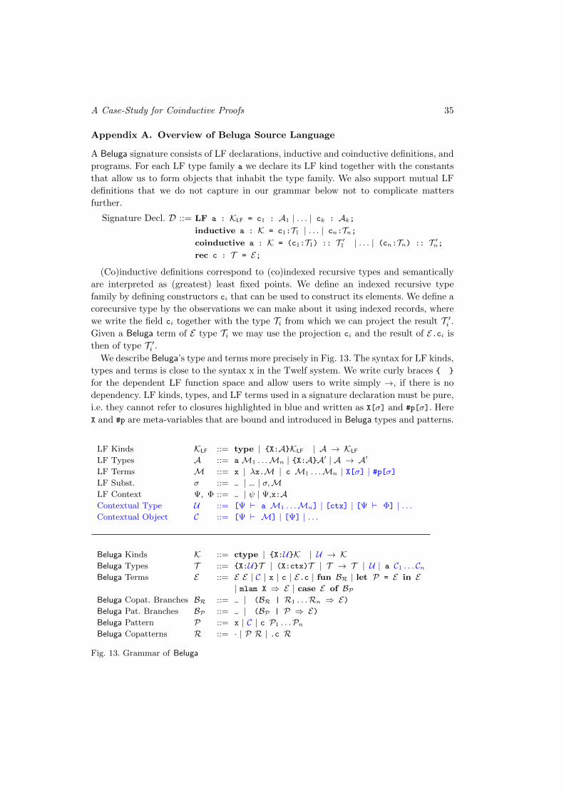
A Case-Study for Coinductive Proofs 35

Appendix A. Overview of Beluga Source Language

A Beluga signature consists of LF declarations, inductive and coinductive definitions, and

programs. For each LF type family a we declare its LF kind together with the constants

that allow us to form objects that inhabit the type family. We also support mutual LF

definitions that we do not capture in our grammar below not to complicate matters

further.

Signature Decl. D ::= LF a : KLF = c1 : A1 | . . . | ck : Ak;inductive a : K = c1:T1 | . . . | cn:Tn;coinductive a : K = (c1:T1) :: T ′1 | . . . | (cn:Tn) :: T ′n;rec c : T = E;

(Co)inductive definitions correspond to (co)indexed recursive types and semantically

are interpreted as (greatest) least fixed points. We define an indexed recursive type

family by defining constructors ci that can be used to construct its elements. We define a

corecursive type by the observations we can make about it using indexed records, where

we write the field ci together with the type Ti from which we can project the result T ′i .

Given a Beluga term of E type Ti we may use the projection ci and the result of E.ci is

then of type T ′i .

We describe Beluga’s type and terms more precisely in Fig. 13. The syntax for LF kinds,

types and terms is close to the syntax x in the Twelf system. We write curly braces { }

for the dependent LF function space and allow users to write simply →, if there is no

dependency. LF kinds, types, and LF terms used in a signature declaration must be pure,

i.e. they cannot refer to closures highlighted in blue and written as X[σ] and #p[σ]. Here

X and #p are meta-variables that are bound and introduced in Beluga types and patterns.

LF Kinds KLF ::= type | {X:A}KLF | A → KLF

LF Types A ::= aM1 . . .Mn | {X:A}A′ | A → A′

LF Terms M ::= x | λx.M | c M1 . . .Mn | X[σ] | #p[σ]LF Subst. σ ::= | ... | σ,MLF Context Ψ, Φ ::= | ψ | Ψ,x:AContextual Type U ::= [Ψ ` a M1 . . .Mn] | [ctx] | [Ψ ` Φ] | . . .Contextual Object C ::= [Ψ ` M] | [Ψ] | . . .

Beluga Kinds K ::= ctype | {X:U}K | U → KBeluga Types T ::= {X:U}T | (X:ctx)T | T → T | U | a C1 . . . CnBeluga Terms E ::= E E | C | x | c | E.c | fun BR | let P = E in E

| mlam X ⇒ E | case E of BPBeluga Copat. Branches BR ::= | (BR | R1 . . .Rn ⇒ E)Beluga Pat. Branches BP ::= | (BP | P ⇒ E)Beluga Pattern P ::= x | C | c P1 . . .PnBeluga Copatterns R ::= · | P R | .c R

Fig. 13. Grammar of Beluga

A. Momigliano, B. Pientka, and D. Thibodeau 36

Substitutions in closures are either empty, written as here, or a weakening substi-

tution ..., which we use in practice to transition from a context to a possible extension.

Substitutions can also be built by extending a substitution σ with a LF term M.

LF contexts may be empty, consists of a context variable, or are built by concatenating

to a LF context a LF variable declaration.

Contextual types and terms pair a LF context together with a LF type or LF term

respectively. As LF contexts are first-class in Beluga, they form valid contextual objects.

LF contexts are in general classified by a schema that allows us to state an invariant the

LF context satisfies; here we only add the one schema we have used in this development

(Section 3.7), namely ctx.

Beluga’s type language supports indexed dependent function space, {X:U}T , non-

dependent functions, embedding contextual types, and (co)inductive definitions, de-

scribed as a C1 . . . Cn. Note that in {X:U}T we make X explicit and hence any computation-

level expression of that type expects first an object of type U . We also permit a limited

form of implicit type annotation for context variables; by writing (X:ctx)T we can ab-

stract over the context variable X and declare its context schema, while keeping X implicit.

Beluga’s computation language allows us to make statements about contextual types

and objects and we highlight them in blue as well. It is in many ways similar to stan-

dard functional programming languages with two exceptions: first, contextual types and

objects are the special domain and we support not only pattern matching, but also copat-

tern matching, i.e., our patterns may include projections describing the observations that

we can make about a given (output) type. In particular, we allow functions to be defined

via (co)pattern matching using the fun keyword. Beluga also supports case analysis us-

ing pattern matching independently for convenience. Further, as in OCaml, we not only

allow functions to be defined via (co)pattern matching, but to be formed by abstracting

over their arguments. For example functions defined using mlam abstract over contextual

variables occurring in the function body. Further, our language features let-expressions

as a degenerate case of case analysis, together with applications, computation-level vari-

ables, constructors, constants, and projections. This is by no means a complete account

of the computation language of Beluga— we have only described here the part relevant

for our case study.