UNIVtRSITVOF

* BOOKSTACKS

s

V-i

oj

£

PD

P

P

«tf

LOr-<C<J

rHOb2

O

«rulinT~»

I

>* o o** 55 ^

^j*

,JH05 lO

PiP^W 0\ T~<

CQ O Oi Oj 00 •

K< O <ffl £m 3= 0-

<n O

f\J r-« O O oo t-

MCMNH

<*m

a in

> JLu or **v in Nin r* •

o oo • P*en m O O

A >4

% HHOS mOn OSM • .

V P ^ P

Pi <

- g

3=3:

X 6 > ac

OO

uu3:

st: BEBR4 COP

FACULTY WORKINGPAPER NO. 89-1554

A Class of Nonlinear Arch Models:

Properties, Testing and Applications

THE LIBRARY OF THE

MAY 3 i 1989

U1jk3aha-champaign

M. L. Higgins

A. K. Bera

College of Commerce and Bush less Administration

Bureau of Economic and Business Research

University of Illinois Urbana-Champaign

BEBR

FACULTY WORKING PAPER NO. 89-1554

College of Commerce and Business Administration

University of Illinois at Urbana -Champaign

April 1989

A Class of Nonlinear Arch Models:

Properties, Testing and Applications

M. L. Higgins

University of Wisconsin-Milwaukee

A. K. Bera, Associate Professor

Department of Economics

Digitized by the Internet Archive

in 2011 with funding from

University of Illinois Urbana-Champaign

http://www.archive.org/details/classofnonlinear1554higg

Revised: April 1989

A CLASS OF NONLINEAR ARCH MODELS: PROPERTIES,TESTING AND APPLICATIONS*

M. L. Higgins

University of Wisconsin-Milwaukee, Milwaukee, WI 53201

and

A. K. Bera

University of Illinois, Champaign, IL 61820

A class of nonlinear ARCH model is suggested. The proposedclass encompasses several functional forms for ARCH which havebeen put forth in the literature. For this more general ARCHmodel, existence of moments are discussed. A Lagrange multipliertest is developed to test Engle ' s ARCH specification against thewider class of models. This test provides an easily computeddiagnostic check of the adequacy of an ARCH model after it hasbeen estimated. Lastly, the theory is applied to specify a

nonlinear ARCH model for the weekly U. S./Canadian dollar exchange

rate

.

* We benefited from the comments of the participants of theAustralasian Meeting of the Econometric Society, Canberra, August28-31, 1988, and the Department of Economics, University ofAlberta, Canada where earlier versions of the paper werepresented. In particular we would like to thank Clive Grangerfor his comments and helpful discussion. We are also indebted toNichola Dyer, Roger Koenker, Dan Nelson and Paul Newbold for manyhelpful suggestions. However, we retain the responsibility forany remaining errors.

'Correspondence should be addressed to M. L. Higgins,Department of Economics, University of Wisconsin-Milwaukee, P.O.Box 413, Milwaukee, WI 53201.

1. Introduction

Since the introduction of the autoregressive conditional

heteroskedasticity (ARCH) model in an influential paper by Engle

(1982), there has been considerable interest in models in which

the variance of the current observation is a function of past

observations. Engle formally defined the ARCH regression model

for a dependent variable yt by specifying its conditional

distribution as

yt |* t_i" N(x

tB,h

t )

where

ht

= h ( Et-l'

£ t-2"--' E t-p;a)

«t

= yt-x

tB,

$ t is the information set at time t, x t is a vector of exogenous

variables and lagged values of the dependent variables, and B and

a are parameter vectors. Engle suggested several functional

forms for h(• ) , but concentrated primarily on the following

linear ARCH model

2 2h. = a +cx.,e:, . + . . . +a e. . (1)t 1 t-1 p t-p v '

To ensure that the conditional variance is strictly positive for

all realizations of e* , the linear ARCH model (1) requires that

the parameter space be restricted to a >0 and a t>0

y i = l,...,p.

Engle showed that if

P1 a. < 1,

i=l2

then the ARCH process is stationary and the unconditional

variance of e t is

2a

Var(et ) = c =

P1 - la.

1=1 l

or

p 2a = (1 - I a )afu

i=l

Substituting this into (1), we have

P 2 2 2h. = (1 - I a.)o +a.E. . +...+a e.t v ._, l ' 1 t-1 p t-p

Therefore, Engle's specification of the conditional variance can

be viewed as a weighted average of the "global" variance o2 and

the "local" variances e2

. _ j , ..., e2

. _ p .

Since Engle's paper, many extensions and generalizations of

the ARCH model have appeared [see Engle and Bollerslev (1986) for

a survey of ARCH models and their applications]. We believe that

this research falls into three general areas, each of which

addresses one of the assumptions of Engle's original ARCH

specification.

First, a majority of research has examined ARCH models in

which the conditional variance h t is a function not only of the

E t 's but also of other elements of # t _,. Weiss (1984, 1986)

suggests ARCH models in which h t is a function of lagged values

of y t , exogenous variables, and predictions of y t based on

elements of the information set f t _!. Engle, Granger and Kraft

(1984) and Granger, Robins and Engle (1982) consider bivariate

time series for which the conditional variance of each series is

3

dependent upon lagged values of the other. Bollerslev (1985)

makes ht also a function of lagged values of itself, i.e.

ht _!,... ,ht _„ , and the resulting model is called the generalized-

ARCH or GARCH model.

A second area of research addresses the assumption of

conditional normality. The conditional distribution of data for

which ARCH models are used, is frequently skewed and leptokurtic.

To account for heavy tails of the conditional distribution, Engle

and Bollerslev (1986) and Bollerslev (1987) examine GARCH models

in which the conditional distribution is assumed to be Student' s-

t rather than normal. For the same reason, Lee and Tse (1988)

suggest using a Gram-Charlier type distribution. It is

difficult, however, to specify a conditional distribution which

allows for both skewness and kurtosis, and still maintain the

tractability of the model. Proper specification of the

conditional distribution of an ARCH process is a question which

warrants further research.

A third extension of the ARCH model, by far the one having

received the least amount of attention to date, considers

functional forms for h t other than Engle 's linear ARCH

specification. Engle (1982) in fact suggested several

functional forms, but concentrated on the linear model for its

analytic convenience and its plausibility as a data generating

mechanism. Engle and Bollerslev (1986) and Geweke (1986) have

suggested other functional forms. The use of alternatives to the

linear ARCH model is hindered by the lack of a specification test

to determine the adequacy of the linear ARCH model and a

procedure for selecting an alternative functional form if the

linear ARCH model is rejected.

The specification of the correct conditional variance

function is important in several respects. The accuracy of

forecast intervals depends upon selecting the function which

correctly relates the future variances to the current information

set. Also, the test for detecting the presence of ARCH is

partially determined by the functional form of the ARCH process.

Further, Pagan and Sabau (1987) have shown that an incorrect

functional form of the ARCH process for the errors of a

regression model can result in inconsistent maximum likelihood

estimators of the regression parameters.

In this paper, we propose a nonlinear ARCH model which

encompasses several of the models which have been proposed in the

literature. Using this more general ARCH model, the

specification testing of the functional form of the ARCH model is

addressed. Section 2 is a survey of functional forms which have

been proposed for ARCH. In Section 3, we introduce a nonlinear

ARCH model and show that it encompasses models discussed in

Section 2. In Section 4, a Lagrange multiplier (LM) test is

developed to test the linear ARCH model against a class of

nonlinear ARCH models. In Section 5, the theory is applied to

specifying a functional form for an ARCH model for the Canadian

weekly exchange rate.

2 . Functional forms for ARCH

Although Engle (1982) focused on the convenient linear ARCH

model, he acknowledged that "it is likely that other formulations

of the variance model may be more appropriate for particular

applications" (p. 993). He suggested two alternatives, the

exponential and absolute value models

ht

= exp(ao+a

iEt-i

+ "- +Vt-p ) <2)

ht " °o

+ail e t-il

+ -- +apl c t-pl- < 3 >

The exponential model (2) has the advantage that the variance is

positive for all values of a; however, as stated by Engle, it has

the unfortunate property that data generated by such a process

will have infinite variance, making estimation and inference

difficult. The absolute value model (3), like the linear model,

requires restrictions on the parameter space to ensure that the

variance is positive. For this model, however, the variance of

the generated data will be finite for all positive parameter

values, a property not shared by the linear ARCH model.

In an empirical application, Engle and Bollerslev (1986)

report having estimated a variety of functional forms for a GARCH

model of the U.S. dollar/Swiss franc exchange rate. They report

results only for the two best models. The ARCH analogues of

these GARCH are

ht = tt

o+a

il E t-ilM+

-

•

- +<I pl Et -il

M< 4 >

and

6

ht

= a +o1(2F( e ^_ 1

/M)-l)+. ..+ap(2F(e^_

p/n)-l) (5)

where F is the cumulative normal distribution. Model (4) is a

simple extension of the absolute value model (3). The model (5)

is an attempt to provide a model in which the conditional

variance h t remains bounded as the values of t\ . L , i=l, . . - ,p,

become arbitrarily large.

Concerned with the non-negativity restrictions on the

parameters of the linear ARCH model, Geweke (1986) suggests the

functional form

2 2log(h

t) = a +a

1log(E

t _ 1)+. . . +o

plog(e

t _p) (6)

which ensures that the conditional variance is positive for all

values of a. Geweke also demonstrates that the log-likelihood

for this ARCH model is globally concave, making maximum

likelihood estimation comparatively easy. Engle and Bollerslev

(1986) criticize this specification, however, because the

likelihood function becomes undefined if a residual of zero is

encountered.

Each of the above models has its individual benefits and

limitations. Clearly any one model cannot be chosen a priori as

the most plausible specification of an ARCH process. Their

usefulness depends upon the particular empirical application.

3 . A general functional form for ARCH

In this section we propose a general functional form for the

ARCH model and then show that this more general model encompasses

models in Section 2.

Consider the ARCH model (2) with

1/6ht =

[v*v *#1 <«ti>

a V et-P

)6

](7)

where

o2

>

i> for i = 0,1, . . . ,p

6 >

and the<f> i 's are such that

PE 0. = 1.

i=0 *

The conditional variance function (7) has p+3 parameters. The

restriction that the ^ 's sum to one reduces the dimension of the

parameter space by one; hence, the model effectively has one more

parameter than Engle's model. The restriction that 6 >0 ensures

that the conditional variance is defined for all c t 's. We will

refer to a model with conditional variance function (7) as a

nonlinear ARCH model of order p, or in short NARCH(p)

.

The function (7) is familiar to economists as the constant

elasticity of substitution (CES) production function of Arrow et

al

.

(1961). If we heuristically view the conditional variance as

output and the "global" and "local" variances as inputs, then the

8

ARCH model has the form of a linear production function with

infinite elasticity of substitution. The NARCH specification, on

the other hand, is very flexible; the elasticity of substitution

1/(1-6) can take values in the range ( 1 , ~ ) for 0<6<1. Equation

(7) could also be written as

l-5 t /-2.6 n ,2.6.. .2.6.,h -1 (a ) -1 (£+._-,) "I < E i--rJ

_1-E_ = +f —Eli + ...+« _E-E

( 8)6 6

X6

P6

which is a Box-Cox (1964) power transformation on both sides of

the Engle (1982) specification. This transformation has been

found to be quite useful in econometric functional form

specification analysis. It has traditionally been used to

linearize otherwise nonlinear models [ see Carroll and Ruppert

(1988, p. 118)]. In time series analysis, Granger and Newbold

(1976) and Hopwood, McKeown and Newbold (1984) have found that

incorporating a power transformation into the ARIMA model is

beneficial in terms of forecast accuracy. Therefore, the NARCH

specification can be expected to improve the estimates of the

forecast intervals. Moreover, as we will see below, the NARCH

form encompasses different conditional heteroskedasticity models

discussed in Section 2, and provides a framework for developing

a specification test for Engle ' s linear ARCH model.

We now show that some of the models of Section 2 are

special cases of the NARCH model (7).

Proposition 1 : The conditional variance function (7) is

equivalent to:

(i) Engle's conditional variance function when 6=1

(ii) Geweke ' s conditional variance function as 6->0.

Proof : The proof of (i) is obvious. Set 6=1 in (7) and let a =

O (a 2) and a i =<fi i , for i=l,...k. To prove (ii), express the NARCH

conditional variance function as (8) and take the limit as 6->0

of both sides, giving

log(ht ) =

olog(o 2

)+01log(e^_

1)+. . .+0

plog(e^_

p)

which is equivalent to Geweke ' s model with a o =0 o log(o2

) and

cii =0 ± , for i=l, . . . ,p.

Here we should note that Geweke ' s model is only a limiting

case of the NARCH model. Imposing the restriction 6>0 allows for

models arbitrarily close to Geweke ' s model, and yet guarantees

that the log-likelihood function is defined. Unfortunately, the

absolute value model (3) is not nested within this general model.

However, the NARCH model can be generalized by including an

additional parameter, in the same way that the constant

elasticity form is generalized to the variable elasticity of

substitution form. The variance function becomes

u/6ht

= k (i2 V 6

. . 2 .6 . . . , 2 ,6

i(e t-i J

+ •••• + V et-P

(9)

Setting both 6=% and u=J$ makes (9) equivalent to the absolute

value model (3). We shall not consider this generalization

further in this paper; rather it is an area for future research.

10

The assumption that the conditional mean of e t is zero

ensures that the unconditional mean and all autocorrelations of

e t are also zero. The nonlinearity of the conditional variance

function makes it difficult to find an explicit expression for

the unconditional variance. We are, however, able to state a

sufficient condition for the unconditional variance of the

NARCH(l) model to be finite.

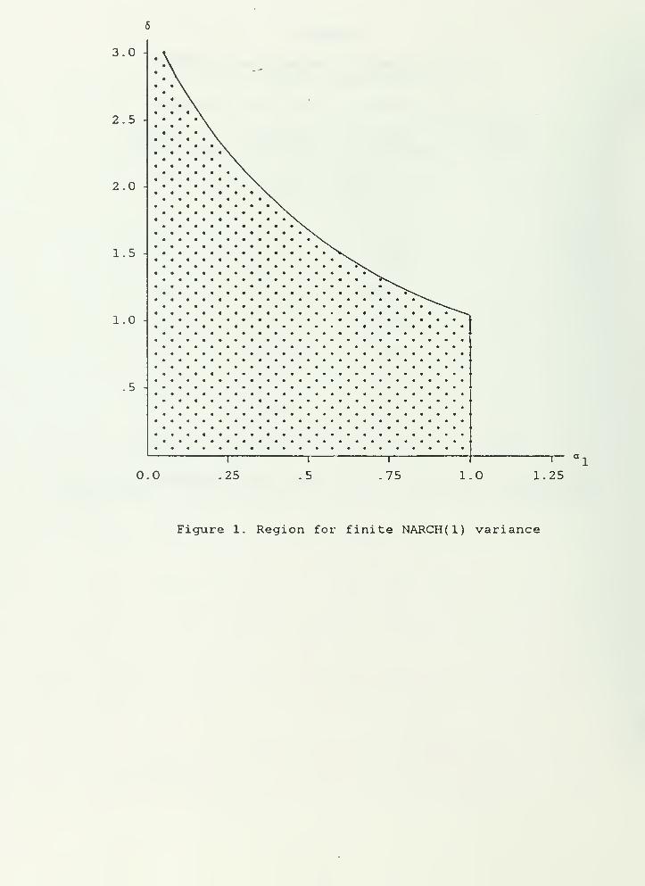
Theorem 1 : The variance of the NARCH(l) model is finite if

where T(') is the gamma function.

The proof of Theorem 1 is given in the Appendix. Extension of

the theorem to the NARCH(p) model is straightforward. The region

for the parameter space for which the variance is finite is shown

in Figure 1.

4. A Lagrange multiplier test for NARCH

Once it has been determined that conditional

heteroskedasticity is present in the data, it is natural to begin

the specification search for functional form with Engle ' s linear

model. It would, therefore, be useful to possess a test to

determine whether Engle 's model provides an adequate description

of the data, or whether a wider class of functional forms for the

conditional variance needs to be considered. In this section we

derive an LM test for Engle s model against the more general

11

class of ARCH models with conditional variance function (7).

Since Geweke ' s model is a member of this class, the test should

have good power against this alternative.

We are interested in testing the hypotheses

Ho :6=1

H, :6/l

in (7), i.e., that Engle's model provides an adequate description

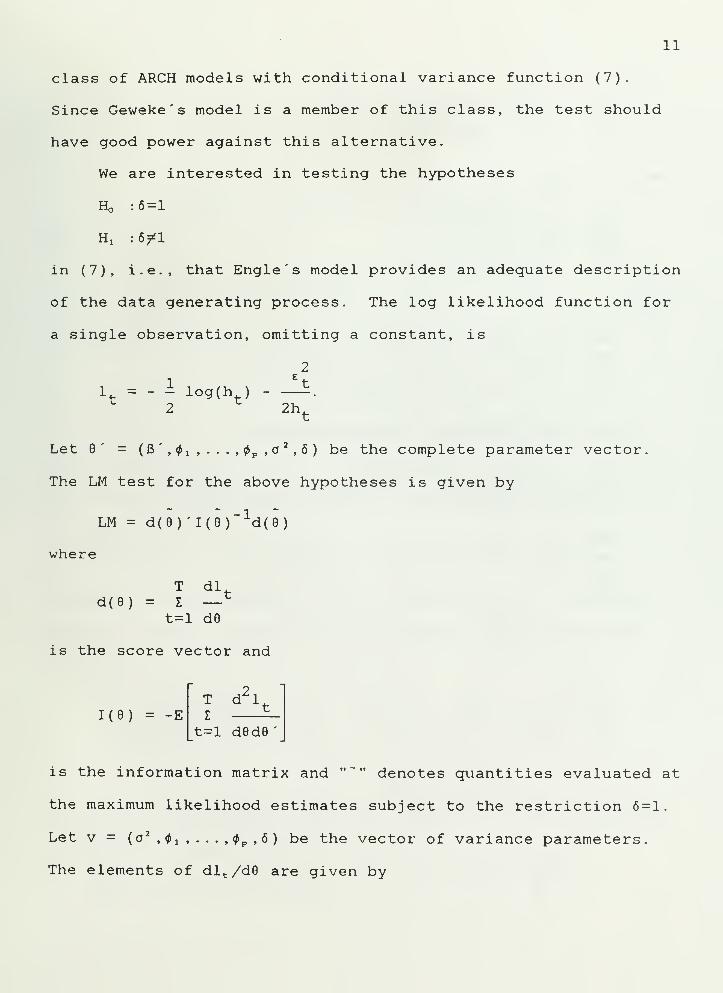
of the data generating process. The log likelihood function for

a single observation, omitting a constant, is

2

1et

I = - ± log(h )H.

2 2ht

Let 8' = (B ' , 0i , . . . , P , a2

, 6 ) be the complete parameter vector.

The LM test for the above hypotheses is given by

LM = d(9) 'I(8)_1

d(8)

where

T dld(8) = Z —

t=l d8

is the score vector and

1(8) = -E

2T d 1

t=l d8d8

is the information matrix and "~" denotes quantities evaluated at

the maximum likelihood estimates subject to the restriction 6=1.

Let v = (a 2, 0! , . . . , <j> p , 6 ) be the vector of variance parameters.

The elements of dl t /d8 are given by

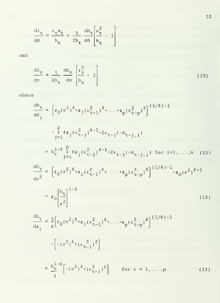
12

dlt

etXt _1_ ^t

dB 2h dB

t— - 1

and

dl

dv

1dh

t

2ht

dv

t— - 1 (10)

where

dh,

dB.l

(•v+M«;_,> 6

+...+v«tp>a

ivt t-i

(l/6)-l

ji1

6 *j ( «tj)6

" 1- 2

't- j <-*t- j .i'

= h1-6 2 ,6-1

dh,

do

I 5<fij(t t_j)•2c

t _j

(-xt _ jj

.) for i=l,...,k (11)

(l/5)-l( °

2)5^l (E

?-l)5+ V«lp>

a * /2.5-1

o(o )

1-6

(12)

dht 1

d0. 6L(.

2)S1 (.t 1>'*-vtp>

,l(1/,)">

-(o2

)

5*(«

t? 1 )

a

1-6 r

it

6

for i = 1 , . . . ,p (13)

13

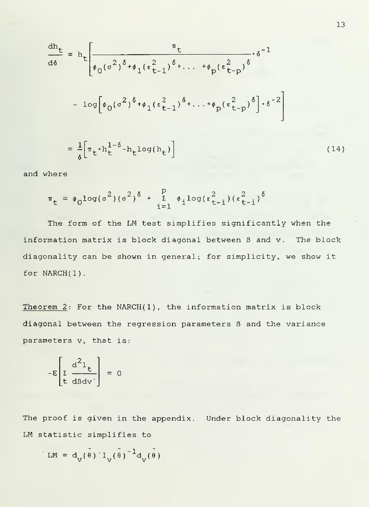
dh,

d6= h,

IT

, 2.6, .2 . 6,

<P(o

) +*1(« t. 1 )

+ r p v t-p'

- log[0o(o

2)

6+0

1(s^_

1)

6 , 2 ,5+. . . +0 (e . )r

pv t-p'

-2

= ^ t' h

t"6 -h

tlog(h

t

and where

(14)

, 2 W 2J % , , 2 . . 2 ,6tt =

Qlog(o )(o ) + I

ilog(e

i)(6 t _ i )

i = l

The form of the LM test simplifies significantly when the

information matrix is block diagonal between B and v. The block

diagonality can be shown in general; for simplicity, we show it

for NARCH(l)

.

Theorem 2 : For the NARCH(l), the information matrix is block

diagonal between the regression parameters R and the variance

parameters v, that is:

-Ed2i

t dBdv=

The proof is given in the appendix. Under block diagonality the

LM statistic simplifies to

lm = d ( e)

' i ( e )

1d ( e

)

V V V

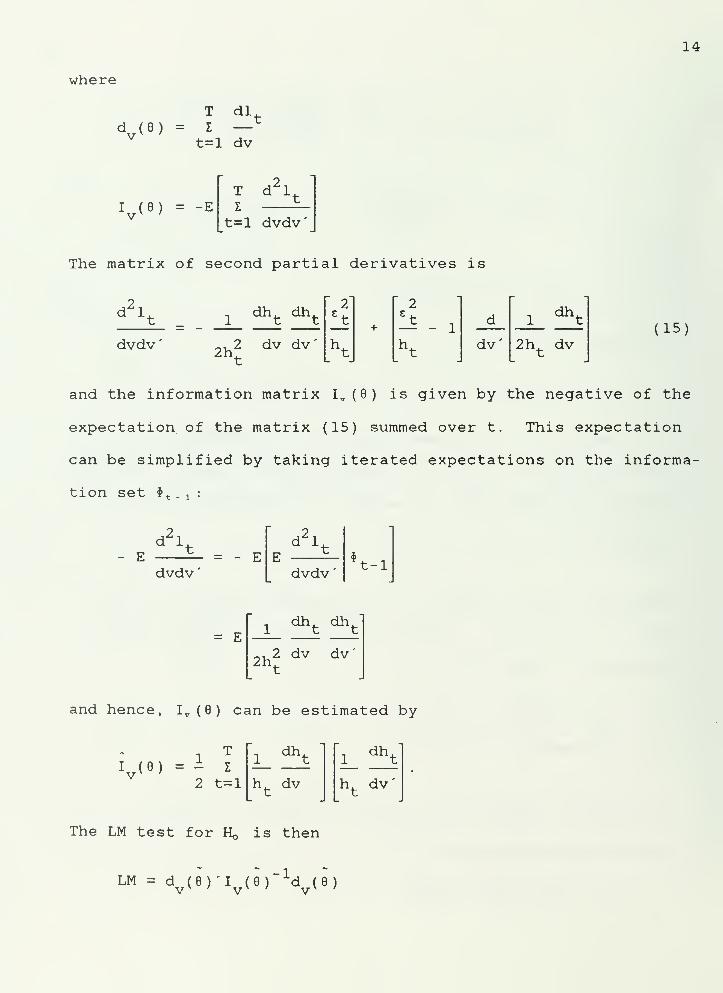
where

T dld (8) = Z —

t=l dv

14

I (9) = -E

2T d 1

t=l dvdv

The matrix of second partial derivatives is

d2i

i ^t ^tdvdv' 2h

2 dv dv'- 1

dv

i ^t2h

tdv

(15)

and the information matrix I v (6) is given by the negative of the

expectation of the matrix (15) summed over t. This expectation

can be simplified by taking iterated expectations on the informa-

tion set $ t _ j :

d2i

- Edvdv

= - Ed2i

dvdv

'

t-1

= E1 ^t ^t

2h2 dv dv

and hence, I v (8) can be estimated by

Iv (6)

= i I

2 t=l h dv2_^h dV

The LM test for H, is then

lm = d ( e)

' i ( e ) *d ( e

)

V V V

15

1

2

t— - 11 ^t

dv

1 ^t

h,dv

i-i-l

Z dv'

Xt— - 1

r dv

The test statistic will be asymptotically distributed as chi-

square with one degree of freedom under the null hypothesis,

we let

~2

If

and

Zt

= i_d*t

: dv

and let f'

=(/ 1 , . .. ,

f

T ) and Z '=(

z

: , . ..

,

z

T ) , the statistic can be

expressed as

LM =2L

I ftzt

-. -lr1 Z

tZt

I ftzt

= Jsf'Z(Z'Z)1Z'f.

This statistic can be computed as J$ the SSR from the regression

of f on Z. Furthermore, since plim(f

' f/T) = 2, an asymptotically

equivalent form of the statistic is

LM = T-f'Z(Z'Z) 1Z'f/f'f

16

which can be computed as T times the uncentered coefficient of

determination from the regression of f on Z.

The test statistic is similar in form to Engle's original LM

test for ARCH. It differs in the function h t and the elements of

dht /dv. In the above test, under the null, h t is the conditional

variance as estimated from Engle's model. The elements of

dht /dv, evaluated under the null hypothesis 6=1, simplify to

^t ~2 ~2= -(a ) + t ._. for i=l,...,p

d0 .

1

dh

2

=*°

doz

d6

where

dh= ir

t- h

tlog(h

t )

2, "2, ? ~2 ,~2

i=l

The test requires estimating Engle's ARCH model and computing the

conditional variance for each observation. It does not, however,

represent a significant computing burden. Presumably, a

researcher has already concluded that ARCH is present in the data

and would naturally proceed by estimating Engle's model. Once

the MLEs of Engle's model are obtained, the test can be performed

on any standard regression package. The test, therefore, should

be viewed as a diagnostic check of the adequacy of Engle's model

after it has been estimated.

17

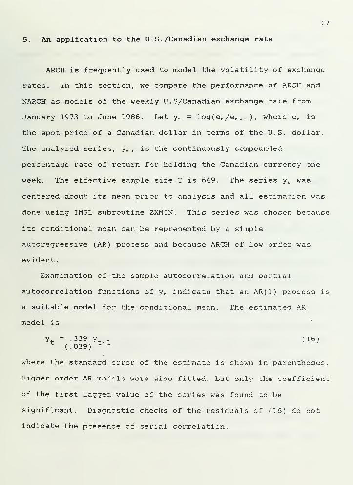
5. An application to the U. S. /Canadian exchange rate

ARCH is frequently used to model the volatility of exchange

rates. In this section, we compare the performance of ARCH and

NARCH as models of the weekly U.S/Canadian exchange rate from

January 1973 to June 1986. Let y t= log(e t /e t . j ), where e t is

the spot price of a Canadian dollar in terms of the U.S. dollar.

The analyzed series, yt , is the continuously compounded

percentage rate of return for holding the Canadian currency one

week. The effective sample size T is 649. The series y t was

centered about its mean prior to analysis and all estimation was

done using IMSL subroutine ZXMIN. This series was chosen because

its conditional mean can be represented by a simple

autoregressive (AR) process and because ARCH of low order was

evident.

Examination of the sample autocorrelation and partial

autocorrelation functions of y t indicate that an AR(1) process is

a suitable model for the conditional mean. The estimated AR

model is

y = .339 y (16)( .039) ^ x

where the standard error of the estimate is shown in parentheses.

Higher order AR models were also fitted, but only the coefficient

of the first lagged value of the series was found to be

significant. Diagnostic checks of the residuals of (16) do not

indicate the presence of serial correlation.

18

The autocorrelations of the squared residuals from (16),

however, reveal that nonlinearity is present. Using the standard

error l/T* = .039 [see Mcleod and Li (1983)], the first

autocorrelation of the squared residuals, .12, is significant at

the 5% level; the rest are insignificant. Engle's LM test for

ARCH was performed for orders 1 through 10. The statistic for

1st order ARCH is highly significant, but the value of the

statistic increases very slightly as additional ARCH terms are

included. Hence, an ARCH(l) model is identified and estimated to

be

yt = -29 yt-i

( .054)

h = .116 + .449 z\? ,

( .01) ( .089)

Log-likelihood function = -332.191

Higher order ARCH models were also fitted, but the additional

ARCH parameters were insignificant.

To determine whether linear ARCH provides an adequate model,

the LM test of Section 4 for NARCH was performed. The computed

value of the test statistic is 6.88, which is highly significant

for a chi-square with one degree of freedom. The estimated

NARCH(l) model is

B o<f>

1

estimate .32 .247 ,255 .148

standarderror 00019 .0257 .0825 .167

Log-likelihood Function = -325.537

19

Initial parameter values for estimating the NARCH were obtained

from the estimated ARCH model, with 6 taken to be 1 as implied by

the linear ARCH specification. The striking feature of the

estimated NARCH model is that 6 falls drastically from 1 to .148.

An asymptotic t-test of the hypothesis that 6 = 1 is easily

rejected. In addition, the likelihood ratio (LR) statistic is

2(332.191-325.537) = 13.308, which is highly significant.

Therefore, all three of the tests, LM, LR and t-test, reject

the linearity imposed by the ARCH model. Table 1 presents the

autocorrelations of the standardized residuals £ t /n^ from the AR,

ARCH and NARCH models; Table 2 presents the autocorrelations of

their squares. For a correctly specified model, these

autocorrelations should be close to zero. Table 1 shows that the

autocorrelations from the NARCH model are closest to zero,

although there is still slight evidence of seventh order

autocorrelation, perhaps due to the weekly nature of the data.

In terms of the autocorrelations of the squares of the

standardized residuals, as we can see from Table 2, clearly the

ARCH model is an improvement over the AR model. Yet additional

improvement, though modest, is apparent when going from the ARCH

to the NARCH model.

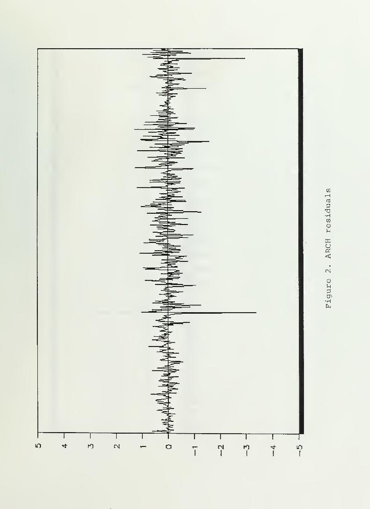
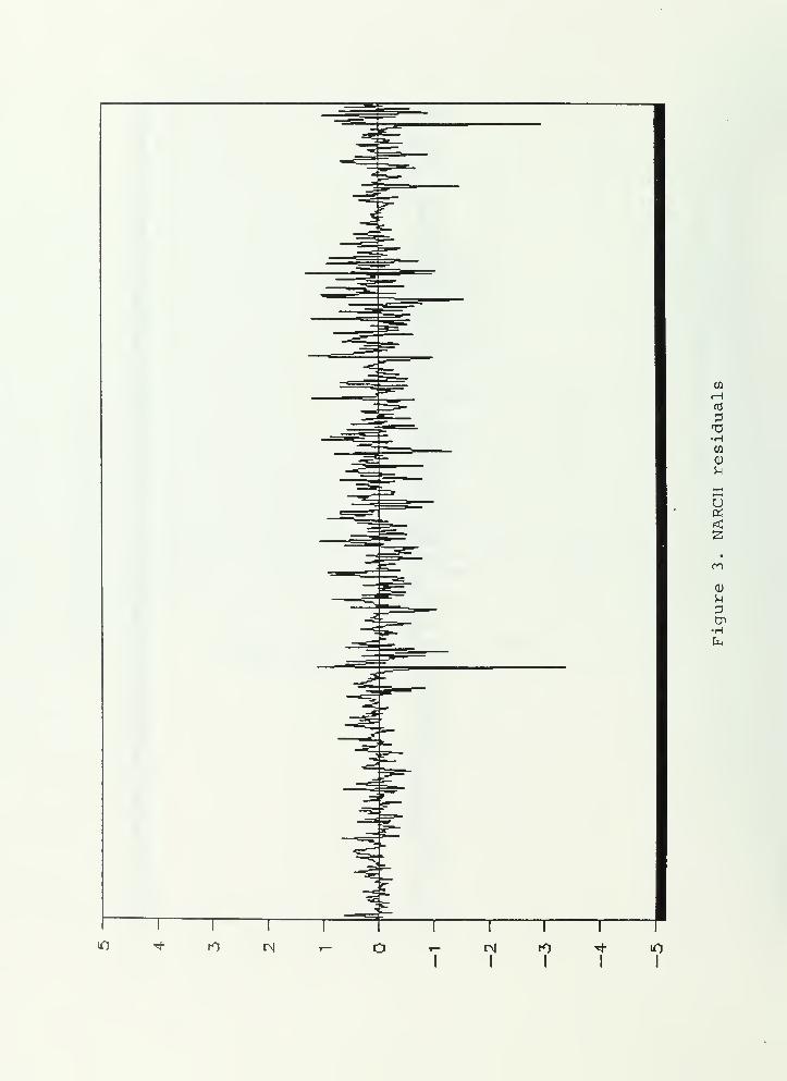
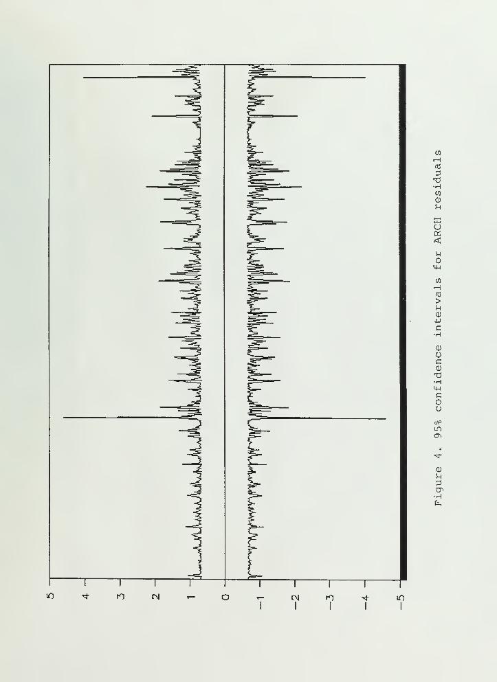
To further compare the performances of ARCH and NARCH, we

plot the residuals and their 95% confidence intervals ±1 . 96(h t)''•

in figures 2-5. From figures 2 and 3, the ARCH and NARCH

residuals are seen to be almost indistinguishable, indicating

that NARCH may not provide a significant improvement over ARCH in

20

terms of the point forecast. The estimated AR parameters for the

two models differ by only .03. The confidence intervals,

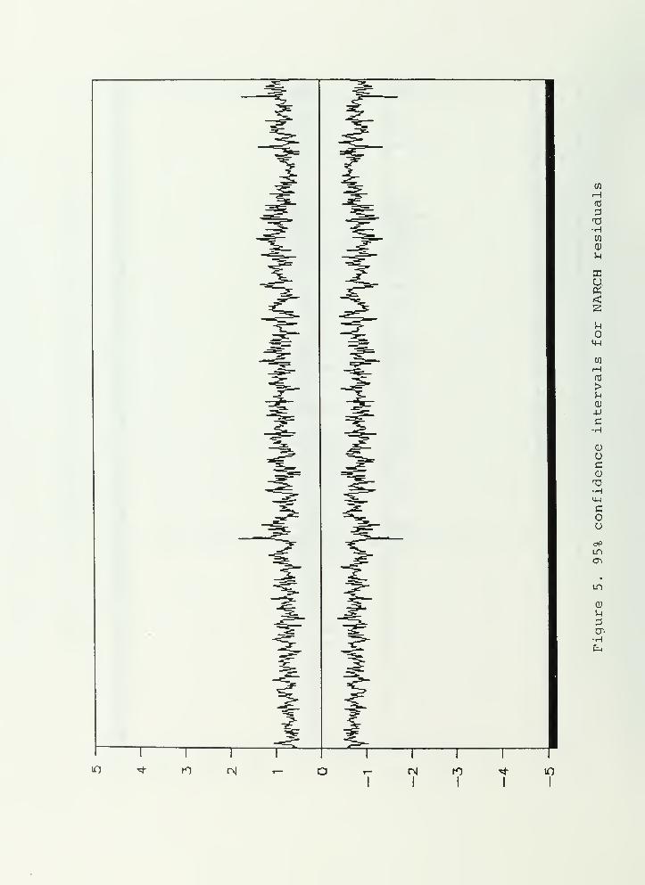
however, are very different. Comparing figures 4 and 5, the

NARCH conditional variances seem to more accurately reflect the

behavior of the series. The confidence intervals of the ARCH

model frequently decline to the lower bound ±1.96(a )!5 = ±.668

during "stable" periods, yet ±.668 is clearly too large an

interval during these periods. On the other hand, during the

"volatile" periods, ARCH seems to frequently overstate the

conditional variance and can vary drastically from one

observation to the next. The confidence intervals of the NARCH

model, however, track the series well. During the stable

periods, the intervals become considerably smaller than the ARCH

intervals. In contrast to the ARCH intervals, the lower bound

for the NARCH intervals is ±1 . 96( *> ' *

o

2)* = ±.360. As should be

expected from a good conditional variance model, we can predict

the series with higher confidence during less volatile periods.

During the volatile periods, the NARCH intervals widen as

required, yet the transition is smooth and not subject to the

erratic variation which occurs for the ARCH intervals.

Summarizing the above results, based on the statistical

tests it appears that a nonlinear model improves the functional

form specification of the conditional variances. Ideally we

would also like the standardized residuals £ t /n* to behave like

white noise and for our model there is "modest" improvement as

indicated by their autocorrelation function. From the plot of

21

the forecast intervals of the residuals, we observe a more

plausible evolution of the conditional variance over time.

22

Appendix

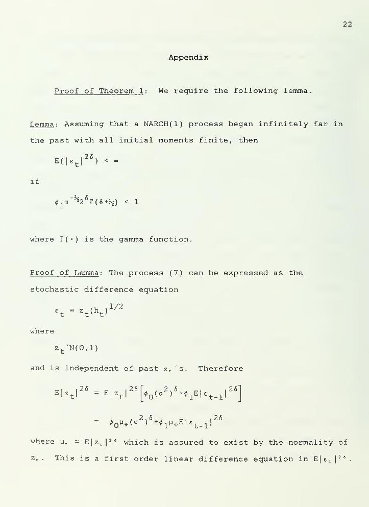
Proof of Theorem 1 : We require the following lemma.

Lemma : Assuming that a NARCH(l) process began infinitely far in

the past with all initial moments finite, then

26(|s

t ru

)<

if

«^

1tt %2 5

T(6+%) < 1

where T(«) is the gamma function.

Proof of Lemma : The process (7) can be expressed as the

stochastic difference equation

1/2et

= zt (V

where

zt~N(0,l)

and is independent of past e t ' s . Therefore

E|et |

26 = E|zt |

26 / 2 . 6 _,i i

2 6<p

Q(o ) ^

1E|e

t _ 1 |

= * M°V +*i^ El

E t-il26

where ^. = E|z t |

2 * which is assured to exist by the normality of

z t . This is a first order linear difference equation in E|e t |

2 *

23

If initial moments are finite, E|E t|

24 will converge to a finite

value if

tfl(i* =

1E|z

t |

26 = # 1»"%2 6

r(6+*j ) < 1

which completes the proof of the lemma.

The condition for the lemma is also sufficient for the

finiteness of the variance. For if 6>1, then

E<«*) = E E(e1

t l*t-l>J

= E, 2.6, .2 .6

*0 (0> ^l^t-l*

-.1/6

(A.l)

2.6 „ i i 2 5

*o<° )

+'i

E K-il-,1/5

where the inequality follows from Jensen's inequality since (A.l)

is a concave function of |

e

t _ a |

2 *. The lemma now assures that

the expectation is finite, and hence the variance is finite. For

5<1, we apply Minkowski's inequality [see White (1984, p.34)], to

establish

E(e£) = E =(«t l

#t-l>

= E,2.6, ,2 .6(o

) ^iCet.i)-,1/6

o(o

2)

6+0

1E(e

t _ 1)

1/6

(A. 2)

24

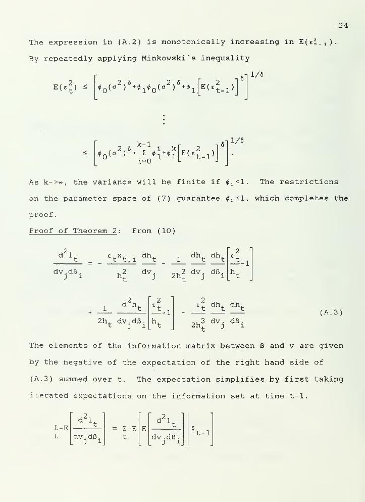
The expression in (A. 2) is monotonically increasing in E(e|_ t ).

By repeatedly applying Minkowski's inequality

E(e^) < ^ o(cJ

2)

6+0

1 o(o

2)

6^1

n 6

E(4-l>

.2.6 „ l^k(o ) • Z 0-!+*-,

i=0B(«J.l)

1/6

As k->~, the variance will be finite if 0!<1. The restrictions

on the parameter space of (7) guarantee 0j<1, which completes the

proof.

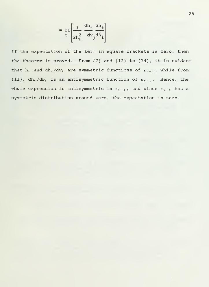
Proof of Theorem 2 : From (10)

d2

i

dv.dB.3 i

e.x. dh,t t , l t

,2 dv.

. dh, dh,1 t t

ov 2 dv . dB .

2ht j i

-1h,

d2h.

2h. dv.dB.t 2 i

--1Et

dht ^t

01 3 dv . dB .

2ht 2 i

(A. 3)

The elements of the information matrix between B and v are given

by the negative of the expectation of the right hand side of

(A. 3) summed over t. The expectation simplifies by first taking

iterated expectations on the information set at time t-1.

Z-Et

d2i

dv .dB.3 i

Z-Et

d2 i

dv .dB

.

3 i

t-1

25

IEt

1 ^t ^t,2 dv.dB.2h

t j i

If the expectation of the term in square brackets is zero, then

the theorem is proved. From (7) and (12) to (14), it is evident

that h t and dh t /dv A are symmetric functions of E t _! , while from

(11), dh t /dJ3i is an antisymmetric function of t i.. 1 . Hence, the

whole expression is antisymmetric in e t _ lf and since e t . j has a

symmetric distribution around zero, the expectation is zero.

26

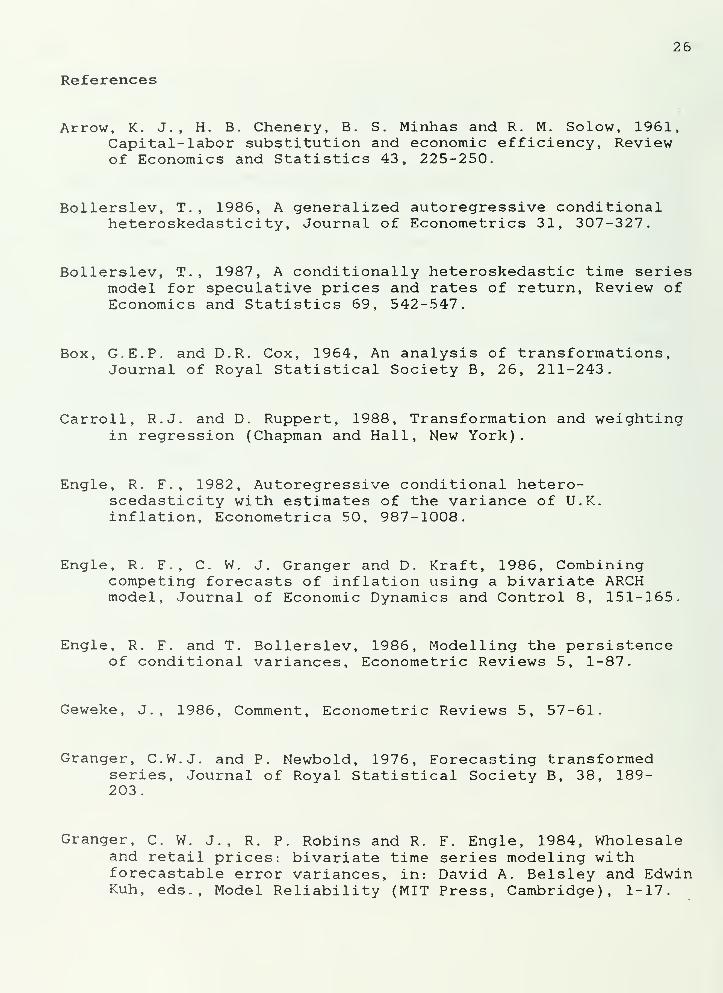
References

Arrow, K. J., H. B. Chenery, B. S. Minnas and R. M. Solow, 1961,Capital-labor substitution and economic efficiency, Reviewof Economics and Statistics 43, 225-250.

Bollerslev, T. , 1986, A generalized autoregressive conditionalheteroskedasticity , Journal of Econometrics 31, 307-327.

Bollerslev, T. , 1987, A conditionally heteroskedastic time seriesmodel for speculative prices and rates of return, Review ofEconomics and Statistics 69, 542-547.

Box, G.E.P. and D.R. Cox, 1964, An analysis of transformations,Journal of Royal Statistical Society B, 26, 211-243.

Carroll, R.J. and D. Ruppert, 1988, Transformation and weightingin regression (Chapman and Hall, New York).

Engle, R. F., 1982, Autoregressive conditional hetero-scedasticity with estimates of the variance of U.Kinflation, Econometrica 50, 987-1008.

Engle, R. F., C. W. J. Granger and D. Kraft, 1986, Combiningcompeting forecasts of inflation using a bivariate ARCHmodel, Journal of Economic Dynamics and Control 8, 151-165

Engle, R. F. and T. Bollerslev, 1986, Modelling the persistenceof conditional variances, Econometric Reviews 5, 1-87.

Geweke, J., 1986, Comment, Econometric Reviews 5, 57-61.

Granger, C.W.J, and P. Newbold, 1976, Forecasting transformedseries, Journal of Royal Statistical Society B, 38, 189-203.

Granger, C. W. J., R. P. Robins and R. F. Engle, 1984, Wholesaleand retail prices: bivariate time series modeling withforecastable error variances, in: David A. Belsley and EdwinKuh, eds., Model Reliability (MIT Press, Cambridge), 1-17.

27

Hopwood, W.S., J.C. McKeown and P. Newbold, 1984, Time seriesforecasting models involving power transformations, Journalof Forecasting, 3, 57-61.

Lee, T. K. Y. and Y. K. Tse, 1988, Term structure of interestrates in the Asian dollar market: ARCH-M Modelling withAutocorrelated Non-normal Errors, mimeograph.

Pagan, A. R. and H. Sabau, 1987, On the inconsistency of the MLEin certain heteroskedastic regression models, mimeograph.

Weiss, Andrew A. , 1984, ARMA models with ARCH errors, Journal ofTime Series Analysis 5, 129-143.

Weiss, Andrew A., 1986, Asymptotic theory for ARCH models:estimation and testing, Econometric Theory 2, 107-131.

White, Halbert, 1984, Asymptotic theory for econometricians(Academic Press, Orlando).

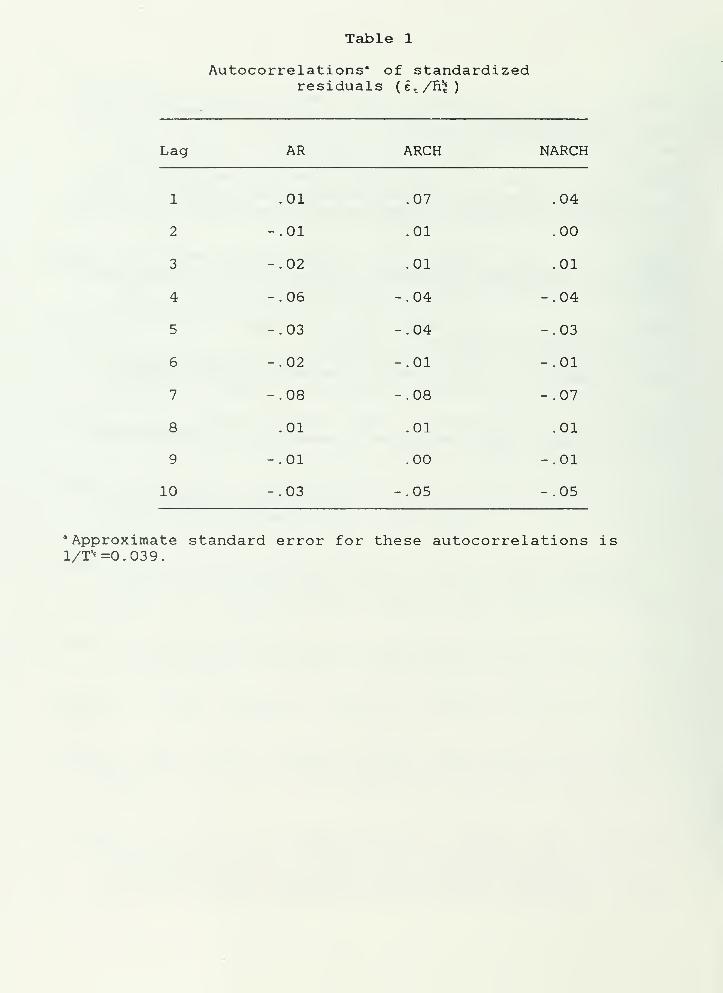
Table 1

Autocorrelations" of standardizedresiduals (e t /n^)

Lag AR ARCH NARCH

.07 .04

.01 .00

.01 .01

-.04 -.04

-.04 -.03

-.01 -.01

-.08 -.07

.01 .01

.00 -.01

-.05 -.05

"Approximate standard error for these autocorrelations isl/T^ =0.039.

1 .01

2 -.01

3 -.02

4 -.06

5 -.03

6 -.02

7 -.08

8 .01

9 -.01

10 -.03

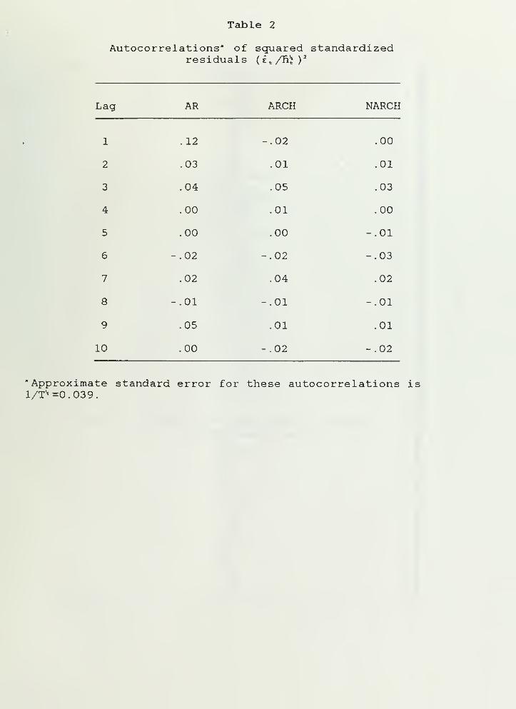
Table 2

Autocorrelations" of squared standardizedresiduals (£ t /n*)

2

Lag AR ARCH NARCH

1 .12 -.02 .00

2 .03 .01 .01

3 .04 .05 .03

4 .00 .01 .00

5 .00 .00 -.01

6 -.02 -.02 -.03

7 .02 .04 .02

8 -.01 -.01 -.01

9 .05 .01 .01

10 .00 -.02 -.02

"Approximate standard error for these autocorrelations is1/1"* =0.039.

3.0

2.5 -

2.0 -

1.5

1.0

0.01—25

~1

—

75 1.0

—r- ai

1.25

Figure 1. Region for finite NARCH(l) variance

wiHrd

3

•HCO

CD

U

CM

<D

5-1

Ptn•H

wi-H

fO

3•O•HCO

<D

a:u<C2

<D

UatnH

en

•H

3

-HWCD

5-1

KU«

5-1

O4-1

03

H>5-1

cd

pc•H

<D

Uc

•H4-1

cou

OPin

0)

5-1

3Cn•H

CO

I—

I

to

3

•HCO

d)

5-1

U.

omCO

i—i

>U0)

4->

c

<u

oc0)

T3-HM-l

cou

af>

inen

0)

uD

-HEn

HECKMANBINDERY INC.