Portland State University Portland State University

PDXScholar PDXScholar

Civil and Environmental Engineering Master's Project Reports Civil and Environmental Engineering

2014

A Comparative Assessment of Crowded Source A Comparative Assessment of Crowded Source

Travel Time Estimates: A Case Study of Bluetooth vs Travel Time Estimates: A Case Study of Bluetooth vs

INRIX on a Suburban Arterial INRIX on a Suburban Arterial

Fahad Alhajri Portland State University

Follow this and additional works at: https://pdxscholar.library.pdx.edu/cengin_gradprojects

Part of the Civil and Environmental Engineering Commons

Let us know how access to this document benefits you.

Recommended Citation Recommended Citation Alhajri, Fahad, "A Comparative Assessment of Crowded Source Travel Time Estimates: A Case Study of Bluetooth vs INRIX on a Suburban Arterial" (2014). Civil and Environmental Engineering Master's Project Reports. 4. https://doi.org/10.15760/CEEMP.25

This Project is brought to you for free and open access. It has been accepted for inclusion in Civil and Environmental Engineering Master's Project Reports by an authorized administrator of PDXScholar. Please contact us if we can make this document more accessible: pdxscholar@pdx.edu.

A COMPARITIVE ASSESSMENT OF CROWDED SOURCE TRAVEL TIME ESTIMATES:

A CASE STUDY OF BLUETOOTH VS INRIX ON A SUBURBAN ARTERIAL

BY

FAHAD F A SH A ALHAJRI

A research project report submitted in partial fulfillment

of the requirement for the degree of

MASTER OF SCIENCE

IN

CIVIL AND ENVIRONMENTAL ENGINEERING

Project Advisor:

Christopher M. Monsere

Portland State University

©2014

ii

ACKNOWLEDGMENTS

I would like to gratefully acknowledge my wonderful advisor Dr. Christopher Monsere whose

support and guidance enabled me to complete this project. It was an honor to work with someone

who really cares about his students.

I would like to also extend my acknowledgement to Jon Makler, Steve Hansen, Joel Barnett at

PSU who contributed to the data collection and analysis of an earlier evaluation on which this

research is based on. Dr. Robert Bertini for coordinating PSU’s access to the INRIX data after

ODOTs approval and support. Dr. Robert Fountain and Alexander Bigazzi for their valuable

input on time series analysis. Ted Trapanier at INRIX for providing helpful orientation on using

the INRIX data for the analysis.

Finally, none of this would have been possible without the unconditional love, endless support

and extraordinary encouragement of my parents, Fawaz and Ahlam, and my aunt Dr. Faiza.

iii

ABSTRACT

Travel time is one of the most widely used measures of traffic performance monitoring for the

transportation systems. It is a simple concept that refers to the time required to traverse between

two points of interest. Travel time is communicated and used by a wide variety of audience such

as commuters, media reporters, and transportation engineers and planners. Recent developments

within the wireless communication area made it possible to collect travel time data at a relatively

low cost. These emerging technologies include mobile phone based technologies, in-vehicle

navigation technologies and automatic vehicle identification technologies. Although these

technologies offer a great collection source for travel time data, they have different levels of

accuracy. In this research two sources of travel time data were evaluated. These sources of data

were the INRIX travel time data and the Bluetooth travel time data. The granularity of the

INRIX and the Bluetooth data were high in which travel time estimates were reported at a one

minute interval. A total of 42 GPS vehicle probe surveys were carried out in three different days

to evaluate the accuracy of the INRIX and the Bluetooth travel time estimates. Statistical

measures such as the mean absolute error (MAE) and the mean absolute percent error (MAPE)

were calculated for a total of 6 segments and 3 time periods (midday, pm peak, and weekend).

The INRIX estimates during the midday were either within 0.36 minutes or 22% of the ground

truth probe runs, while the Bluetooth estimates during the pm peak were either within 1 minute

or 24% of the ground truth probe runs. In addition to hypothesis testing for 13,541 matched-pairs

observation, correlation testing was carried out to evaluate the behavior of the Bluetooth and

INRIX time series.

iv

TABLE OF CONTENTS

1.0 INTRODUCTION .................................................................................................................................. 1

2.0 LITERATURE REVIEW ....................................................................................................................... 3

3.0 STUDY AREA ........................................................................................................................................ 7

4.0 DATA… .................................................................................................................................................. 8

4.1 Benchmark ............................................................................................................................................... 8

4.2 ODOT Bluetooth ...................................................................................................................................... 8

4.3 INRIX… ................................................................................................................................................ 10

5.0 DATA PROCESSING .......................................................................................................................... 12

5.1 Temporal Alignment of Segments ........................................................................................................... 12

5.2 Spatial Alignment of Segments ............................................................................................................... 12

6.0 RESULTS ............................................................................................................................................. 15

6.1 Bluetooth – Probe Comparison ................................................................................................................ 17

6.2 INRIX – Probe Comparison .................................................................................................................... 18

6.3 Bluetooth – INRIX Comparison .............................................................................................................. 20

Difference in Travel Time Means...................................................................................................... 20

Correlations .................................................................................................................................... 22

7.0 CONCLUSIONS ................................................................................................................................... 25

8.0 REFERENCES ..................................................................................................................................... 26

APPENDICES

A Travel Time Profiles……………………………………………………………………………….29

B CCF Correlograms………………………………………………………………………….…......36

v

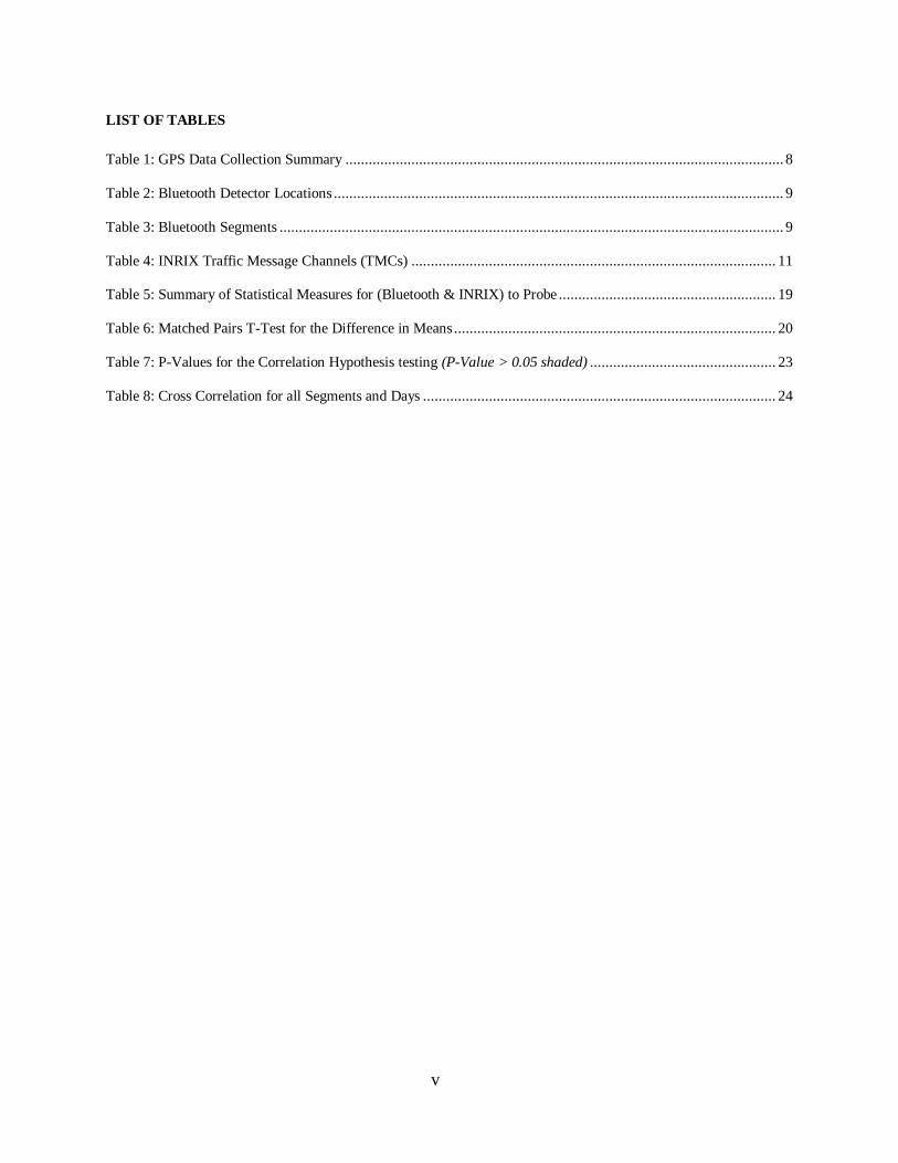
LIST OF TABLES

Table 1: GPS Data Collection Summary ................................................................................................................. 8

Table 2: Bluetooth Detector Locations .................................................................................................................... 9

Table 3: Bluetooth Segments .................................................................................................................................. 9

Table 4: INRIX Traffic Message Channels (TMCs) .............................................................................................. 11

Table 5: Summary of Statistical Measures for (Bluetooth & INRIX) to Probe ........................................................ 19

Table 6: Matched Pairs T-Test for the Difference in Means ................................................................................... 20

Table 7: P-Values for the Correlation Hypothesis testing (P-Value > 0.05 shaded) ................................................ 23

Table 8: Cross Correlation for all Segments and Days ........................................................................................... 24

vi

LIST OF FIGURES

Figure 1: Utility Benfit vs Travel Time Accuracy .................................................................................................... 3

Figure 2: Bluetooth Data Collection Method ........................................................................................................... 4

Figure 3: Study Area with Bluetooth and INRIX Segments ..................................................................................... 7

Figure 4: INRIX Fusion Engine ............................................................................................................................ 10

Figure 5: Aligning Start and End Point of Segments .............................................................................................. 12

Figure 6: OR 99W Study Segments....................................................................................................................... 14

Figure 7: Sample Time Series Plots (4/1/2014)...................................................................................................... 16

Figure 8: Probe Travel Time vs Estimates Travel Time ......................................................................................... 21

Figure 9: Time Series Profile of McDonald to Durham (4/1/2014) ......................................................................... 22

Figure 10: CCF Correlogram for McDonald to OR-217 (4/1/2014) ........................................................................ 24

Figure 11: Travel Time Profiles for Southbound Segments (4/1/2014) ................................................................... 30

Figure 12: Travel Time Profiles for Northbound Segments (4/1/2014) ................................................................... 31

Figure 13: Travel Time Profiles for Southbound Segments (4/3/2014) ................................................................... 32

Figure 14: Travel Time Profiles for Northbound Segments (4/3/2014) ................................................................... 33

Figure 15: Travel Time Profiles for Southbound Segments (4/5/2014) ................................................................... 34

Figure 16: Travel Time Profiles for Northbound Segments (4/5/2014) ................................................................... 35

Figure 17: CCF Correlogram for I-5 to OR-217 .................................................................................................... 37

Figure 18: CCF Correlogram for OR-217 to McDonald ......................................................................................... 38

Figure 19: CCF Correlogram for McDonald to Durham ........................................................................................ 39

Figure 20: CCF Correlogram for Durham to McDonald ........................................................................................ 40

Figure 21: CCF Correlogram for McDonald to OR-217 ......................................................................................... 41

Figure 22: CCF Correlogram for OR-217 to I-5 .................................................................................................... 42

1

1.0 INTRODUCTION

Travel time is one of the most widely used measures of traffic performance monitoring for the

transportation systems. It is a simple concept that refers to the time required to traverse between

two points of interest. Travel time is communicated and is used by a wide variety of audience

such as commuters, media reporters, and transportation engineers and planners. Commuters use

travel time to locate their housing with respect to their work location. The media reports an

expected delay in travel time along a freeway when an incident takes place. Engineers and

planners use travel time to evaluate transportations facilities and quantify capital investment.

Traditionally, the level of service (LOS) as in the Highway Capacity Manual (HCM) and

AASHTO Geometric Design of Highways and Streets measured the performance of a

transportation facility. The LOS assigns letters “A” through “F” to a transportation facility, “A”

as being best and “F” as being worst. During the development of the level of service, the

availability of transportation data was very limited. Presently, the Intelligent Transportation

Systems (ITS) deployments and the infiltration of new technologies into the market made it

possible to immensely increase the availability of transportation data. These technologies fall

into one of two categories the first being fixed-point technologies and the second being probe

vehicle technologies (Tantiyanugukchai, 2004).

Fixed-point technologies (Inductive loop detectors, CCTV Cameras, and Automatic Vehicle

Identification) collect various traffic characteristics of a stream at predetermined points where

the sensors are installed. Probe vehicle technologies are vehicles infused into the traffic stream

with a capability of recording position and time data (GPS receiver) while in the stream. The

data is then downloaded and synthesized to obtain traffic measures such as travel time and travel

speed of the transportation system (Izadpanah, 2010).

Recent developments within the wireless communication area made it possible to collect traffic

data at a relatively low cost. These emerging technologies include mobile phone based

technologies, in-vehicle navigation technologies and automatic vehicle identification

technologies. The mobile phone based technologies tracks the position of a mobile phone

through cellular towers or GPS receivers impeded in the phones. The in-vehicle navigation

technologies track the position of vehicles using GPS receivers, which are then transmitted to a

2

server. The server receives the positions of the vehicle through either cellular network

automatically or manually when the owner connects the navigation device to the Internet for

updating purposes. The automatic vehicle identification (AVI) technologies covers a large

spectrum of technologies such as radio frequency identification (RFID), automatic license plate

recognition, Bluetooth … etc. In all of the AVI technologies the vehicle is identified upstream at

location “A” and the timestamp is recorded. The vehicle is then identified again downstream at

location “B” and a timestamp is recorded. The difference between a timestamp recorded at

location “A” and a timestamp recorded at location “B” is the travel time spent by the vehicle to

travel between point “A” and “B” (Izadpanah and Hellinga, 2007).

Although previously mentioned technologies offer a great collection source for travel time data,

they have different levels of accuracy. There have been very few side-by-side assessments and

comparative analyses conducted for these technologies. As a result, the objective of this study

was to compare the INRIX travel time data to the traditional Bluetooth travel time data. The

granularity of the INRIX and the Bluetooth data were high in which travel time estimates were

reported at a one minute interval. The study area for this research is approximately a 4.2-mile

section of a suburban arterial (Oregon route 99W). GPS vehicle probe surveys were carried out

in three different days to evaluate the accuracy of the INRIX and the Bluetooth travel time

estimates. Statistical measures such as the mean absolute error (MAE) and the mean absolute

percent error (MAPE) were calculated for a total of 6 segments and 3 time periods (midday, pm

peak, and weekend). Hypothesis testing for 13,541 matched-pairs observation was conducted to

determine whether or not the travel time collected by the Bluetooth method significantly differ

from the INRIX method. Moreover, correlation testing was carried out to evaluate the behavior

of the Bluetooth and INRIX time series.

This research is organized as follows: (1) Literature review provides a summary of the efforts in

evaluating the travel time data; (2) Study area describes the location where the datasets were

collected; (3) Data describes the datasets which were used in this research; (4) Data processing

describes the methodology used in preparing the datasets; (5) Results present the outcome of the

evaluation; (6) Conclusion summarizes the findings of this research.

3

2.0 LITERATURE REVIEW

The reliability and accuracy of technologies that predicts travel time is important to road users.

Toppen and Wunderlich (2003) studied the relationship between the error in travel time and the

utility benefit to road users. The results of the study showed that when the accuracy drops below

a certain threshold, the users are better off using their own travel experience than to use the travel

time predicted by the Advanced Travelers Information Systems. The relationship depicting the

utility gained by travelers with respect to the error in travel time estimation for the case study is

shown in Figure 1. The x-axis represent the percent error in travel time, while the y-axis

represent the per trip utility in dollars. The curves represent the utility gained by the trip maker at

four time periods: am peak in dark blue, pm peak in green, off peak in light blue, and all time

period in red. For a 25 minute perfect trip (0% error), the trip maker was determined to realize a

$2.00 utility. From the figure, an error ranging between 13% and 21% results in a negative

utility. In this research the acceptable threshold for the error was defined to be 25%.

Figure 1: Utility Benfit vs Travel Time Accuracy

Source: Toppen and Wunderlich (2003)

4

The Bluetooth technology has become the new source for travel time estimation due its cost

effectiveness. Vehicles with electronic devices (cell phones, vehicle radios, PCs… etc.) that are

equipped with Bluetooth technology emit waves that can be detected by Bluetooth receivers.

These emissions are detected only when the device is set to discovery mode. Each device

equipped with Bluetooth technology has a specific anonymous identifier called a Media Access

Control (MAC) address. By placing two Bluetooth detectors, one at the beginning of the segment

and one at the end of it, a timestamp is recorded when vehicles are entering the segment and

when vehicles are leaving it. The matching of a specific MAC address associated with a vehicle

at the entry and exit is used to calculate the travel time for that vehicle. An overview of the

Bluetooth technology is presented in Figure 2. The accuracy and reliability of the Bluetooth

technology for the purpose of travel time estimation is a topic discussed by several authors

(Wasson et al. (2008), Qyale et al. (2010), Malinovskiy et al. (2010), Haghani et al. (2010), and

Araghi et al. (2012)).

Figure 2: Bluetooth Data Collection Method

Source: Haghani et al. (2009)

5

Few studies were conducted to assess and evaluate the quality of vehicle probe data at a high

level of detail. Haghani et al. (2009) from the University of Maryland validated the INRIX data

for the I-95 corridor. The evaluation was carried out by comparing the INRIX data to ground

truth data. Their evaluation followed three stages: (1) collect ground truth data, (2) establish the

statistical measures for comparison of INRIX GPS data to ground truth, and (3) compare the data

to ground truth and draw conclusions. In the process of collecting the ground truth data they

ruled out the traditionally floating car method. They decided not to use the traditional floating car

method because it would have been very costly to apply in their large network (1500 miles of

freeway and 1000 miles of arterials). Instead of using the floating car method they used the

Bluetooth technology.

Since the Bluetooth method of collecting travel time data is fairly a new method, Haghani et al.

(2009) validated its accuracy by comparing it to ground truth data collected by GPS Probe

vehicle runs. The comparison was performed by conducting a statistical hypothesis test to

determine whether or not the means speeds collected by the Bluetooth method significantly

differ from the mean speeds collected from floating car runs. A total of nine days of floating car

testing was performed in the states of Maryland and North Virginia as a base to determine the

accuracy of the Bluetooth data. The result of the statistical analysis showed the Bluetooth data to

be a consistent and accurate for field measurement of travel times. The Bluetooth data was then

used to evaluate the INRIX GPS data. For the purpose of the statistical analysis, the speed was

broken down into 4 bins: 0 to 30 mph, 30 to 45 mph, 45 to 60 mph, and greater than 60 mph.

Haghani et al. (2009) used the average absolute speed error (ASSE) and the speed error bias

(SEB) as a statistical measures to compare the INRIX data to the Bluetooth data. They found that

the INRIX data fell within the SEM band, the ASSE value to be less than 10 mph, and the SEB

value to less than 5 mph. It was then concluded that the INRIX travel time and speed data to

have a satisfying accuracy.

The Minnesota DOT compared the INRIX travel time data to loop detector data on an urban

freeway. The INRIX travel time was found most accurate during peak periods and at speeds

nearing the posted speed limit. The evaluation showed that 98% of the INRIX travel time

estimates fell within 2 minutes or 20% of the loop detector travel times (MnDOT, 2012).

Moreover, the Washington DOT conducted a study to evaluate the accuracy and reliability of

6

several ATIS technologies on I-90 (rural freeway) and SR 522 (urban arterial). In the study, the

automatic license plate reader (ALPR) system was used to evaluate the accuracy of the Bluetooth

and INRIX travel time estimates. Measures such as Mean Absolute Deviation (MAD), Mean

Absolute Error (MAE), and Mean Absolute Percent Error (MAPE) were calculated to assess the

accuracy of the estimates. The results of the study showed the Bluetooth estimate to have a lower

MAPE value than the INRIX estimates over the course of the day. The Bluetooth displayed

lower accuracy during the night where sampling was really low. Futhermore, The Bluetooth and

INRIX estimates were examined on a segment for a time period with a road closure. The

Bluetooth continued on reporting the travel time for 30 minutes after road closure, while the

INRIX failed to show a reaction to road closure. It was concluded from the study that the

Bluetooth had a higher overall reliable travel time than the INRIX (WSDOT, 2014).

7

3.0 STUDY AREA

The study area of this research is approximately a 4.2-mile section of the State Highway 99W

corridor between the Durham Road/OR 99W intersection at the south end and the I-5 interchange

at the north end. Highway 99W is 5 lanes wide and at minimum 4 lane wide at some sections.

The posted speed limit in the corridor is between 35 and 40 mph. The highway carries

approximately 38,000 vehicles a day with 1.50% heavy vehicles (ODOT, 2013). The corridor is

surrounded by a variety of land uses with the majority being retail and commercial services. A

map showing the corridor (purple), the Bluetooth segment boundaries (blue) and the INRIX

TMC boundaries (green) is presented in Figure 3

Figure 3: Study Area with Bluetooth and INRIX Segments

N

8

4.0 DATA

In this study two data sources were used:

Bluetooth, and

INRIX

The GPS vehicle probes were used as a benchmark to evaluate the accuracy of these data

sources. The GPS probe vehicle survey was conducted by the ITS lab at Portland State

University. The Bluetooth travel time data was obtained from the Oregon Department of

Transportation System and the INRIX Travel Time data was provided by INRIX under a license

purchased by ODOT. The following subsection will describe each dataset.

4.1 Benchmark

In order to obtain ground truth data, a total of 42 GPS probe runs were carried out in three-time

periods: midday, pm peak, and weekend. The data was collected on Tuesday 4/1/2014, Thursday

4/3/2014, and Saturday 4/5/2014. The GPS probe runs followed the floating car methodology

outlined in the FHWA Travel Time Data Collection Handbook (FHWA, 1998). A detailed

summary of the collection effort is presented in Table 1.

Table 1: GPS Data Collection Summary

Date Day of Week Start End Hours Time Period Total Number of Runs

4/1/2014 Tuesday 12:00 14:00 2 Midday 11

4/1/2014 Tuesday 16:00 18:00 2 PM Peak 9

4/3/2014 Thursday 12:00 14:00 2 Midday 4

4/3/2014 Thursday 16:00 18:00 2 PM Peak 8

4/5/2014 Saturday 11:00 13:00 2 Weekend 10

Total 10 42

4.2 ODOT Bluetooth

The Bluetooth travel time data was retrieved from 5 Bluetooth detectors in the study area. Each

Bluetooth detector records the MAC address and the timestamp associated with each travelling

vehicles containing a Bluetooth device set to discovery mode. The location of these Bluetooth

Detectors along Oregon route 99W are presented in Table 2

9

Table 2: Bluetooth Detector Locations

Detector ID Detector Location Mile Post Latitude Longitude

467 99W / I-5 7.58 N 45.44326 W 122.74279

468 99W / OR-217 8.55 N 45.43568 W 122.75995

469 99W / Main 9.46 N 45.42893 W 122.77569

470 99W / McDonald 10.39 N 45.41856 W 122.78755

471 99W / Durham 11.49 N 45.40456 W 122.79645

Once the MAC address is matched between two consecutive detectors, a travel time is calculated

for the traversed segment between the detectors. The Oregon DOT system uses data collection

devices designed by Kim and Porter (Porter and Kim, 2011). Since there are 5 detectors in the

study area there are 4 segments in each direction. The Bluetooth travel time data that was

obtained from Oregon DOT’s own system contains attributes such as: a timestamp, a segment ID

and an average travel time for that segment. The Bluetooth segments are summarized in Table 3.

Table 3: Bluetooth Segments

Direction Segment ID Segment Begins Segment Ends Segment Length (miles)

So

uth

bo

un

d 2293 I-5 OR-217 0.97

2295 OR-217 Main 0.91

2297 Main McDonald 0.93

2299 McDonald Durham 1.10

No

rth

bo

un

d 2300 Durham McDonald 1.10

2298 McDonald Main 0.93

2296 Main OR-217 0.91

2294 OR-217 I-5 0.97

The Bluetooth data was available at a high resolution and the travel time estimates were reported

at a one-minute interval. For each minute interval, the travel time estimate is an average of all

vehicles observed for that minute interval. Moreover, the data processing of the outliers to

generate travel times is done by the Oregon DOT software.

10

4.3 INRIX

INRIX is a private party that collects information about the roadway conditions. It accomplishes

this mission with its smart drive network that aggregates nearly 400 sources of data. Sources of

data with regards to flow and traffic incidents include: road sensors, traffic cameras, commercial

vehicle GPS probes, consumer vehicle GPS probes, cellular network probes, road crashes, and

road construction. Once the source-aggregated traffic data is collected, it then gets processed

using a proprietary data fusion engine. An overview of the INRIX total fusion engine is

presented in Figure 4. INRIX currently covers busy streets, arterials, major freeways, and the

entire interstate system. It is combining real-time, historical and predictive traffic data for more

than 800,000 miles across the United States (INRIX Inc., 2014).

Figure 4: INRIX Fusion Engine

Source: INRIX Inc.

11

A corridor in the INRIX data is comprised of multiple segments called Traffic Message Channels

(TMCs). Table 4 presents a list of specific TMCs selected for the study area. Performance

measures such as real time speed, travel time, and confidence score are recorded for each TMC.

The possible confidence score reported for the INRIX readings listed from highest to lowest are

30, 20, and 10. These three levels are interpreted as following:

“30” – Completely based on real-time data.

“20” – Based on a combination of real-time and historical data.

“10” – Completely based on historical data.

Table 4: INRIX Traffic Message Channels (TMCs)

Direction TMC Begins Ends Length (miles)

So

uth

bo

un

d

114-07920 SW Gaard St SW Durham 0.81

114-07919 OR-217 Off-ramp SW McDonald 1.68

114-07918 I-5 Off-ramp OR-217 Off-ramp 1.01

No

rth

bo

un

d

114+07921 OR-217 Off-ramp SW Coronado St 0.81

114+07920 SW McDonald St OR-217 On-Ramp 1.67

114+07919 SW Durham St SW Gaard St 1.01

12

5.0 DATA PROCESSING

5.1 Temporal Alignment of Segments

Since there was a total of 4 Bluetooth segments in each travelling direction and a total of 3

INRIX segments in the study area, The Bluetooth segments had to be reduced to 3 segments.

This was accomplished by summing up the travel time of two consecutive Bluetooth segments in

each direction to create a new longer segment r by using the following expression:

𝑇𝑇𝑟 (𝑡) = ∑ 𝑇𝑇𝑖(𝑡) ∀ 𝑡 ∈ 𝑇

𝑆

𝑖=1

(1)

Where,

TTi = Average travel time for segment i during time interval t

TTr = Average travel time for the new combined segment r during time interval t

S = {Segments to be combined}

5.2 Spatial Alignment of Segments

The Bluetooth segments and the INRIX segments were then plotted on a map and it was evident

in some areas that the INRIX segment starting and ending points did not fully align with the

Bluetooth segment starting and ending points. In order to make a one-to-one comparison, the

segments starting and ending points needed to be completely matching. This was resolved by

altering the INRIX segments. Figure 5 is a scenario used in explaining the process used to

correct for the spatial alignment.

Figure 5: Aligning Start and End Point of Segments

INRIX Segment

Bluetooth Segment

Start End End

13

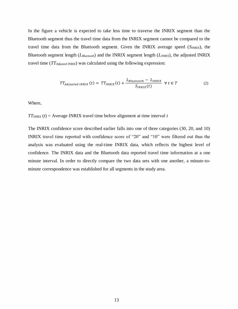
In the figure a vehicle is expected to take less time to traverse the INRIX segment than the

Bluetooth segment thus the travel time data from the INRIX segment cannot be compared to the

travel time data from the Bluetooth segment. Given the INRIX average speed (SINRIX), the

Bluetooth segment length (LBluetooth) and the INRIX segment length (LINRIX), the adjusted INRIX

travel time (TTAdjusted INRIX) was calculated using the following expression:

𝑇𝑇𝐴𝑑𝑗𝑢𝑠𝑡𝑒𝑑 𝐼𝑁𝑅𝐼𝑋 (𝑡) = 𝑇𝑇𝐼𝑁𝑅𝐼𝑋 (𝑡) + 𝐿𝐵𝑙𝑢𝑒𝑡𝑜𝑜𝑡ℎ − 𝐿𝐼𝑁𝑅𝐼𝑋

𝑆𝐼𝑁𝑅𝐼𝑋(𝑡) ∀ 𝑡 ∈ 𝑇 (2)

Where,

TTINRIX (t) = Average INRIX travel time before alignment at time interval t

The INRIX confidence score described earlier falls into one of three categories (30, 20, and 10)

INRIX travel time reported with confidence score of “20” and “10” were filtered out thus the

analysis was evaluated using the real-time INRIX data, which reflects the highest level of

confidence. The INRIX data and the Bluetooth data reported travel time information at a one

minute interval. In order to directly compare the two data sets with one another, a minute-to-

minute correspondence was established for all segments in the study area.

14

Figure 6: OR 99W Study Segments

15

6.0 RESULTS

The 4.2-miles of OR 99W corridor was broken down into six segments as shown in Figure 6. For

each segment and each time period (Midday, PM Peak, and Weekend), the Bluetooth data as

well as the INRIX data were compared to the benchmark. An example of the post-processed data

is shown in Figure 7. The figure shows the travel time estimates of the Bluetooth system plotted

in blue, the INRIX system plotted in green, and the probe travel times for the same traversals as

black squares for one day, April 1, 2014. Similar data were used to compare each probe run was

paired with its equivalent Bluetooth and INRIX reading. The basis of the comparison for the

Bluetooth-to-probe data and INRIX-to-probe data were quantitative (statistical) and qualitative

(graphical). For the quantitative analysis, the mean absolute error (MAE) in minutes and the

mean absolute percent error (MAPE) values were calculated for each segment and time period.

The MAPE values were produced using the following procedure:

1. Each probe run is paired with its equivalent estimated travel time (Bluetooth and INRIX).

2. The difference between the probe travel time and the estimated travel time is then divided

by the probe travel time to calculate the percent error.

3. The absolute value of the percent error is then average over each time period (midday,

pm peak, and weekend) to create a single MAPE value for that time period.

Since the MAPE value shows the magnitude of the error but fails to show the direction of the

error, the average error in minutes was calculated for each time period of each segment. Based

on the direction of the error (positive or negative), the following categories were created:

a) Overestimated

Bluetooth travel time > probe travel time.

INRIX travel time > probe travel time.

b) Underestimated

Bluetooth travel time < probe travel time.

INRIX travel time < probe travel time

16

Figure 7: Sample Time Series Plots (4/1/2014)

17

Furthermore, statistical hypothesis tests (Equations 3 and 4) for all segments and time periods

were conducted to evaluate the accuracy of travel time estimates. Unlike the recorded travel time

of the probe vehicle that was based on a single vehicle, the Bluetooth and the INRIX travel time

are averages of multiple vehicles for a single time interval. Therefore, the results obtained from

the hypothesis test were considered of a high bar. The null hypothesis in these statistical tests

state that there is no difference between the mean travel time estimates (𝜇𝐵𝑙𝑢𝑒𝑡𝑜𝑜𝑡ℎ and 𝜇𝐼𝑁𝑅𝐼𝑋)

and the mean probe travel time (𝜇𝑃𝑟𝑜𝑏𝑒).

The statistical hypothesis testing was performed at a level of confidence (α) equal to 0.05.

6.1 Bluetooth – Probe Comparison

The results of the Bluetooth comparison to the probe data is shown in Table 5. The mean

absolute error results show that the Bluetooth travel time is most accurate during the pm peak

period and least accurate during the midday period. The average error ranges from a low of 0.61

minutes for the Durham to McDonald section on the weekend to a high of 1.94 minutes for the

McDonald to OR-217 section on the weekend.

It is important to note that the segments are relatively short (approximately 1 mile), thus the

percent error can be high. Based on the MAPE values, the travel time estimates during the pm

peak period is most accurate and the weekend period is least accurate. The MAPE value ranges

from a low of 11.86% for OR-217 to McDonald segment on the weekend to a high of 57.26% for

I-5 to OR-217 section on weekend.

To find the direction of the error (overestimated or underestimated), the average error values

were calculated and the overestimated runs were separated from the underestimated runs. The

percent of overestimated runs were calculated by dividing the number of overestimate runs by

(Null Hypothesis) 𝐻0 ∶ 𝜇𝐵𝑙𝑢𝑒𝑡𝑜𝑜𝑡ℎ − 𝜇𝑃𝑟𝑜𝑏𝑒 = 0 (3)

(Alternative Hypothesis) 𝐻1 ∶ 𝜇𝐵𝑙𝑢𝑒𝑡𝑜𝑜𝑡ℎ − 𝜇𝑃𝑟𝑜𝑏𝑒 ≠ 0

(Null Hypothesis) 𝐻0 ∶ 𝜇𝐼𝑁𝑅𝐼𝑋 − 𝜇𝑃𝑟𝑜𝑏𝑒 = 0 (4)

(Alternative Hypothesis) 𝐻1 ∶ 𝜇𝐼𝑁𝑅𝐼𝑋 − 𝜇𝑃𝑟𝑜𝑏𝑒 ≠ 0

18

the total number of runs. The results show that the majority of the Bluetooth estimates were

overestimated.

At a 95th confidence level, a p-value less than 0.05 indicates that there was a statistical

significance difference in travel time between the Bluetooth data and the ground truth data.

Likewise, p-values larger than 0.05 indicate insufficient evidence to conclude a difference. The

pm peak travel times are most accurate and the midday travel times are least accurate. During the

pm peak period only 2 out 6 segments witnessed a significant difference.

6.2 INRIX – Probe Comparison

The results of the INRIX comparison to the probe data is shown in Table 5. The mean absolute

error results show that the INRIX travel time was most accurate during the Midday with all

segments having mean absolute error of less than a minute. The average error ranges from a low

of 0.15 minutes for the McDonald to OR-217 section on the Midday to a high of 7.6 minutes for

the McDonald to OR-217 section on the weekend. Moreover, the Durham to McDonald segment

experienced accurate travel time for all time periods.

Based on the MAPE values, the midday period is most accurate having 5 out of 6 segments with

MAPE value less than 25%. The MAPE value ranges from a low of 11.86% for OR-217 to

McDonald segment on the weekend to a high of 57.26% for I-5 to OR-217 section on weekend.

In addition, the OR-217 to McDonald segment experiences an MAPE value less of less than 25%

across all time periods.

The overestimation percentage results indicate that the INRIX estimates were all underestimated.

Moreover, results of the p-value from the matched pairs t-test show the midday estimates to be

most accurate, while the weekend estimates to be least accurate. Table 5 represents a summary of

the statistical measures discussed for both the Bluetooth and the INRIX travel time estimates.

19

Table 5: Summary of Statistical Measures for (Bluetooth & INRIX) to Probe

Mean Absolute Error in Minutes (MAE < 1.00 shaded)

Direction Segment Segment Name Bluetooth INRIX

Midday PM Peak Weekend Midday PM Peak Weekend

Southbound

1 I-5 to OR-217 1.18 1.18 1.36 0.21 2.83 0.76

2 OR-217 to McDonald 1.54 1.16 0.68 0.16 1.35 1.42

3 McDonald to Durham 1.08 0.74 1.03 0.21 1.34 0.63

Northbound

1 Durham to McDonald 1.05 0.92 0.61 0.69 0.87 0.92

2 McDonald to OR-217 1.32 0.98 1.94 0.15 0.91 7.60

3 OR-217 to I-5 0.85 0.62 0.92 0.36 0.87 1.10

Mean Absolute Percent Error (MAPE < 25% shaded)

Direction Segment Segment Name Bluetooth INRIX

Midday PM Peak Weekend Midday PM Peak Weekend

Southbound

1 I-5 to OR-217 44.4% 25.2% 57.6% 21.5% 39.9% 27.3%

2 OR-217 to McDonald 31.9% 22.4% 11.9% 15.9% 20.6% 24.5%

3 McDonald to Durham 47.7% 16.1% 46.4% 21.1% 33.1% 21.9%

Northbound

1 Durham to McDonald 45.7% 41.7% 19.5% 24.3% 34.3% 26.5%

2 McDonald to OR-217 27.2% 20.9% 13.2% 15.0% 17.6% 54.1%

3 OR-217 to I-5 30.1% 20.3% 31.7% 36.3% 26.7% 30.7%

Percent of Overestimated Travel Time (Overestimate > 50% shaded)

Direction Segment Segment Name Bluetooth INRIX

Midday PM Peak Weekend Midday PM Peak Weekend

Southbound

1 I-5 to OR-217 100% 59% 90% 13% 0% 30%

2 OR-217 to McDonald 75% 71% 75% 0% 0% 13%

3 McDonald to Durham 87% 41% 89% 33% 0% 22%

Northbound

1 Durham to McDonald 71% 50% 89% 36% 44% 11%

2 McDonald to OR-217 100% 75% 33% 29% 6% 0%

3 OR-217 to I-5 79% 63% 78% 14% 6% 0%

P-Values for Matched Pairs T-Test (P-Value > 0.05 shaded)

Direction Segment Segment Name Bluetooth INRIX

Midday PM Peak Weekend Midday PM Peak Weekend

Southbound

1 I-5 to OR-217 0.00 0.47 0.01 0.45 0.00 0.79

2 OR-217 to McDonald 0.01 0.01 0.08 0.00 0.00 0.12

3 McDonald to Durham 0.01 0.43 0.03 0.48 0.00 0.35

Northbound

1 Durham to McDonald 0.02 0.06 0.06 0.07 0.59 0.07

2 McDonald to OR-217 0.00 0.01 0.09 0.22 0.00 0.00

3 OR-217 to I-5 0.04 0.08 0.03 0.01 0.00 0.00

20

6.3 Bluetooth – INRIX Comparison

In Figure 8, the matched pairs of the travel time runs for all of the segments and time periods

evaluated are shown. In the Figure, the y-axis represents the probe travel time and the x-axis

represents the crowd sourced travel time. The Bluetooth estimates are shown in blue; the INRIX

estimates in green. If all estimates were equal, they would fall on the dashed line in the figure.

The plots reinforce the analysis in Table 5, that the INRIX data that tends to underestimate travel

times and the Bluetooth data tends to overestimate travel times.

Difference in Travel Time Means

To determine whether the travel time obtained from the Bluetooth data was similar or different

from the travel time obtained from the INRIX data, a matched-pairs t-test was conducted. A total

of 13,541 observation from three days (4/1/2014, 4/3/2014, and 4/5/2014) were used as an input

for the matched-pairs t-test. The null hypothesis in the statistical test (Equation 5) was that there

was no difference between the Bluetooth mean travel time (𝜇𝐵𝑙𝑢𝑒𝑡𝑜𝑜𝑡ℎ) and the INRIX mean

travel time (𝜇𝐼𝑁𝑅𝐼𝑋) in each time interval.

(Null Hypothesis) 𝐻0 ∶ 𝜇𝐵𝑙𝑢𝑒𝑡𝑜𝑜𝑡ℎ − 𝜇𝐼𝑁𝑅𝐼𝑋 = 0 (5)

(Alternative Hypothesis) 𝐻1 ∶ 𝜇𝐵𝑙𝑢𝑒𝑡𝑜𝑜𝑡ℎ − 𝜇𝐼𝑁𝑅𝐼𝑋 ≠ 0

The statistical hypothesis testing was performed at a level of confidence (α) equal to 0.05. The

matched pairs t-test for the entire dataset (13,541 observations) showed sufficient evidence to

conclude that the difference between the Bluetooth mean travel time and the INRIX mean travel

time was significant. The mean of the differences was found to be 1.87 minutes, thus suggesting

the Bluetooth mean travel time was significantly higher than the INRIX mean travel time. The

results of the hypothesis test is presented in Table 6

Table 6: Matched Pairs T-Test for the Difference in Means

Pair

Paired Differences

T stat df P-value

(2-tailed) Mean Standard

Deviation

95% Confidence Interval

Lower Upper

µBluetooth-µINRIX 1.867 1.589 1.840 1.894 136.67 13540 0.00

21

Figure 8: Probe Travel Time vs Estimates Travel Time

22

Correlations

In Figure 9, a sample of time series plot is shown for the INRIX and the Bluetooth data. In the

figure the y-axis represents the travel time estimate and the x-axis represents the time of day. The

bluetooth estimates are shown in blue, and the INRIX estimates are shown in green. It can be

noticed from the figure that the both data sets have a relatively matching increasing and

decreasing trends.

Figure 9: Time Series Profile of McDonald to Durham (4/1/2014)

A correlation is a dimensionless statistical measure of linear association between a pair of

variables. The correlation takes on a value between -1 and +1. A value of 0 indicates no linear

association, while a -1 and +1 indicate a perfect linear association. A positive value indicates a

positive linear association, likewise a negative value indicates a negative linear association. The

correlation of a population (ρ) is expressed by:

𝜌(𝑥, 𝑦) =

𝐶𝑜𝑣 (𝑥, 𝑦)

𝜎𝑥𝜎𝑦

(6)

23

Where,

Cov = Covariance of the pair (x, y)

σx = Standard deviation of x

σy = Standard deviation of y

To better understand the magnitude of the similarity in trends, a hypothesis test for the

population correlation (ρ) was conducted. The null hypothesis in the statistical test (Equation 7)

was that correlation between the Bluetooth and INRIX pairs is equal to zero.

(Null Hypothesis) 𝐻0 ∶ 𝜌 = 0

(7)

(Alternative Hypothesis) 𝐻1 ∶ 𝜌 ≠ 0

At a 95th confidence level, a p-value less than 0.05 indicates that that the Bluetooth time series is

correlation to the INRIX time series. Likewise, p-values larger than 0.05 indicate insufficient

evidence to conclude an existence of a correlation. The results of the hypothesis test showed

sufficient evidence to conclude that the Bluetooth and INRIX time series are correlated for all

segments and days with the exception of McDonald to Durham section on Saturday, and OR-217

to I-5 section on Tuesday and Saturday. The p-values for all segments by day are summarized in

Table 7.

Table 7: P-Values for the Correlation Hypothesis testing (P-Value > 0.05 shaded)

Direction Segment Segment Name Time Period (7:00 – 19:00)

Tuesday Thursday Saturday

Southbound

1 I-5 to OR-217 0.00 0.00 0.00

2 OR-217 to McDonald 0.00 0.00 0.00

3 McDonald to Durham 0.00 0.00 0.05

Northbound

1 Durham to McDonald 0.00 0.00 0.00

2 McDonald to OR-217 0.00 0.00 0.00

3 OR-217 to I-5 0.11 0.00 0.51

24

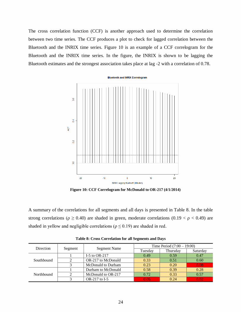
The cross correlation function (CCF) is another approach used to determine the correlation

between two time series. The CCF produces a plot to check for lagged correlation between the

Bluetooth and the INRIX time series. Figure 10 is an example of a CCF correlogram for the

Bluetooth and the INRIX time series. In the figure, the INRIX is shown to be lagging the

Bluetooth estimates and the strongest association takes place at lag -2 with a correlation of 0.78.

A summary of the correlations for all segments and all days is presented in Table 8. In the table

strong correlations (ρ ≥ 0.40) are shaded in green, moderate correlations (0.19 < ρ < 0.49) are

shaded in yellow and negligible correlations (ρ ≤ 0.19) are shaded in red.

Table 8: Cross Correlation for all Segments and Days

Direction Segment Segment Name Time Period (7:00 – 19:00)

Tuesday Thursday Saturday

Southbound

1 I-5 to OR-217 0.49 0.59 0.47

2 OR-217 to McDonald 0.33 0.51 0.60

3 McDonald to Durham 0.23 0.20 0.08

Northbound

1 Durham to McDonald 0.58 0.39 0.28

2 McDonald to OR-217 0.72 0.33 0.57

3 OR-217 to I-5 0.06 0.24 0.02

Figure 10: CCF Correlogram for McDonald to OR-217 (4/1/2014)

25

7.0 CONCLUSIONS

In this research the INRIX travel time data was compared to the traditional Bluetooth travel time

estimates. The INRIX data was found to be most accurate during the midday period, while the

Bluetooth data was found most accurate during the pm peak period. The INRIX estimates during

the midday were either within 0.36 minutes or 22% of the ground truth probe runs. The

Bluetooth estimates during the pm peak were either within 1 minute or 24% of the ground truth

probe runs. Unlike the INRIX data that tends to underestimate travel times, the Bluetooth data

tends to overestimate travel times.

The matched pairs t-test for 13,541 observations showed the Bluetooth estimates to be

significantly different from the INRIX estimates. The hypothesis test for the population

correlation (ρ) showed sufficient evidence to conclude that the Bluetooth and INRIX time series

are correlated for almost all segments and days. The CCF correlograms validated the existence of

a moderate to strong correlation when the INRIX was lagging the Bluetooth estimates. The result

of this study demonstrated that satisfying accurate travel time estimates could be obtained from

both the Bluetooth and the INRIX datasets.

From this study, it is suggested that future research need to be conducted on other corridor with

different characteristics. This study was limited by its focus on three days’ worth of data, which

could be better improved in terms of confidence by expanding on the size and number of days

for the collected data. The merging of the INRIX and the Bluetooth dataset is a promising

futuristic step towards improving the accuracy and reliability of travel time estimation.

26

8.0 REFERENCES

Araghi, Bahar N., Kristian S. Pedersen, Lars T. Christensen, Rajesh Krishnan, and Harry

Lahrmann. (2012) Accuracy of Travel Time Estimation Using Bluetooth Technology: A

Case Study Limfjord Tunnel Aalborg. 19th ITS World Congress.

Athey Creek Consultant. (2012). Evaluation of Arterial Real-Traveler Information Commercial

Probe Data Project. Prepared for MnDOT.

Federal Highway Administration (FHWA). (1998). Travel Time Data Collection Handbook.

FHWA-PL98-035.

Haghani A., Hamedi M., and Sadabadi K. (2009) I-95 Corridor Coalition Vehicle Probe Project:

Validation of INRIX Data July-September 2008. University of Maryland. College Park,

MD.

Haghani, A., Hamedi, M., Sadabadi, K.F., Young, S.E., and Tarnoff, P.J. (2010) Freeway Travel

Time Ground Truth Data Collection Using Bluetooth Sensors. In Proceedings 89th

Annual Meeting Transportation Research Board, Washington.

INRIX Incorporated. INRIX Total Fusion.

http://www.inrix.com/pdf/INRIX%20Total%20Fusion.pdf. Accessed July 20, 2014.

Izadpanah, P., and Hellinga, B. (2007). Wide-Area Wireless Traffic Condition Monitoring:

Reality or Wishful Thinking?, the 2007 CITE Annual Conference in Toronto, Ontario.

Izadpanah, P., (2010). Freeway Travel Time Prediction Using Data from Mobile Probes. Ph.D.

Thesis, Department of Civil and Environmental Engineering, University of

Waterloo,Ontario.

Mainovskiy, Y., Wu, Y.J., Wang, Y., Lee, U.K. (2009). Field Experiments on Bluetooth-Based

travel time data collection. In Preceedings 89th Annual Meeting Transportation Research

Board, Washington.

Oregon Department of Transportation (ODOT) Transportation Data Unit. (2013). 2012

Transportation Volume Tables.

Porter, J. D., Kim, D. S., and Magana, M. E. (2011) Wireless Data Collection System for Real-

Time Arterial Travel Time Estimates (No. OR-RD-11-10).

Quayle, S., Koonce P., J.V., Bullock, D.M., and DePencier, D. (2010). Arterial Performance

Measures Using MAC Readers: Pilot Study in Portland Oregon. In Proceedings 89th Annual

Meeting Transportation Research Board, Washington.

Tantiyanugulchai, S. (2004). Arterial Performance Measurement Using Transit Buses as Probe

Vehicles. M.S. Thesis, Department of Civil and Environmental Engineering, Portland

State University, OR.

27

Toppen A and Wunderlich K. (2003). Travel time data collection for measurement of advanced

Traveler information systems accuracy. Federal Highway Administration, Project No.

0900610-D1. 20 p.

Washington Department of Transportation (WSDOT) (2014). Error Assessment for Emerging

Traffic Data Collection Devices (WA-RD 810.1).

Wasson, J., Sturdevant, J., and Bullock, D.M. (2008). Real-Time Travel Time estimates using

Media Access Control Address Matching, ITE Journal, vol. 78, pp.20-23.

28

APPENDICES

29

APPENDIX A

Travel Time Profiles

30

Figure 11: Travel Time Profiles for Southbound Segments (4/1/2014)

31

Figure 12: Travel Time Profiles for Northbound Segments (4/1/2014)

32

Figure 13: Travel Time Profiles for Southbound Segments (4/3/2014)

33

Figure 14: Travel Time Profiles for Northbound Segments (4/3/2014)

34

Figure 15: Travel Time Profiles for Southbound Segments (4/5/2014)

35

Figure 16: Travel Time Profiles for Northbound Segments (4/5/2014)

36

APPENDIX B

CCF Correlograms

37

Figure 17: CCF Correlogram for I-5 to OR-217

38

Figure 18: CCF Correlogram for OR-217 to McDonald

39

Figure 19: CCF Correlogram for McDonald to Durham

40

Figure 20: CCF Correlogram for Durham to McDonald

41

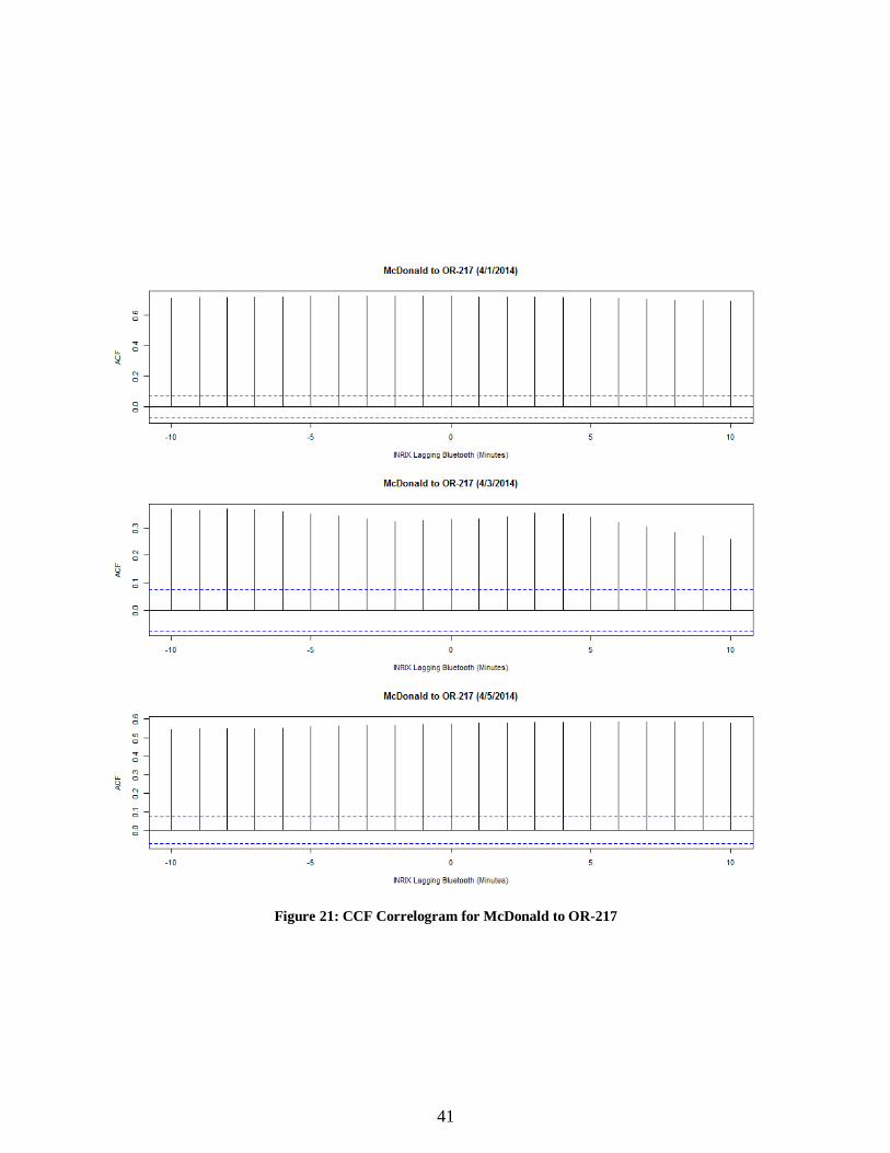
Figure 21: CCF Correlogram for McDonald to OR-217

42

Figure 22: CCF Correlogram for OR-217 to I-5