A comparative experimental study on the use of Acoustic

1

A comparative experimental study on the use of Acoustic Emission and vibration analysis for bearing defect identification and estimation of defect

size

Abdullah M. Al-Ghamd1, D. Mba2 1Mechanical Services Shops Department, Saudi Aramco, Dhahran, Saudi Arabia

2School of Engineering, Cranfield University, Bedfordshire. MK43 0AL, UK

Abstract

Vibration monitoring of rolling element bearings is probably the most established diagnostic

technique for rotating machinery. The application of Acoustic Emission (AE) for bearing

diagnosis is gaining ground as a complementary diagnostic tool, however, limitations in the

successful application of the AE technique have been partly due to the difficulty in

processing, interpreting and classifying the acquired data. Furthermore, the extent of bearing

damage has eluded the diagnostician. The experimental investigation reported in this paper

was centered on the application of the Acoustic Emission technique for identifying the

presence and size of a defect on a radially loaded bearing. An experimental test-rig was

designed such that defects of varying sizes could be seeded onto the outer race of a test

bearing. Comparisons between AE and vibration analysis over a range of speed and load

conditions are presented. In addition, the primary source of AE activity from seeded defects

is investigated. It is concluded that AE offers earlier fault detection and improved

identification capabilities than vibration analysis. Furthermore, the AE technique also

provided an indication of the defect size, allowing the user to monitor the rate of degradation

on the bearing; unachievable with vibration analysis.

Keywords: Acoustic Emission, bearing defect, condition monitoring, defect size, vibration

analysis.

LI2106

Text Box

Mechanical Systems and Signal Processing, Volume 20, Issue 7, October 2006, Pages 1537-1571.

2

1. Introduction

Acoustic emissions (AE) are defined as transient elastic waves generated from a rapid release

of strain energy caused by a deformation or damage within or on the surface of a material [1].

In this particular investigation, AE’s are defined as the transient elastic waves generated by

the interaction of two surfaces in relative motion. The interaction of surface asperities and

impingement of the bearing rollers over the seeded defect on the outer race will generate

AE’s. Due to the high frequency content of the AE signatures typical mechanical noise (less

than 20kHz) is eliminated.

2. Bearing defect diagnosis and Acoustic Emissions

There have been numerous investigations reported on applying AE to bearing defect

diagnosis. Roger [2] utilised the AE technique for monitoring slow rotating anti-friction slew

bearings on cranes employed for gas production. In addition, successful applications of AE

to bearing diagnosis for extremely slow rotational speeds have been reported [3, 4]. Yoshioka

and Fujiwara [5, 6] have shown that selected AE parameters identified bearing defects before

they appeared in the vibration acceleration range. Hawman et al [7] reinforced Yoshioka’s

observation and noted that diagnosis of defect bearings was accomplished due to modulation

of high frequency AE bursts at the outer race defect frequency. The modulation of AE

signatures at bearing defect frequencies has also been observed by other researchers [8, 9,

10]. Morhain et al [11] showed successful application of AE to monitoring split bearings with

seeded defects on the inner and outer races.

This paper investigates the relationship between AE r.m.s, amplitude and kurtosis for a range

of defect conditions, offering a more comparative study than is presently available in the

public domain. Moreover, comparisons with vibration analysis are presented. The source of

3

AE from seeded defects on bearings, which has not been investigated to date, is presented

showing conclusively that the dominant AE source mechanism for defect conditions is

asperity contact. Finally a relationship between the defect size and AE burst duration is

presented, the first known detailed attempt.

3. Experimental Test Rig and Test Bearing

The bearing test rig employed for this study had an operational speed range of 10 to 4000rpm

with a maximum load capability of 16kN via a hydraulic ram. The test bearing employed

was a Cooper split type roller bearing (01B40MEX). The split type bearing was selected as it

allowed defects to be seeded onto the races, furthermore, assembly and disassembly of the

bearing was accomplished with minimum disruption to the test sequence, see figure 1.

Characteristics of the test bearing (Split Cooper, type 01C/40GR) were:

o Internal (bore) diameter, 40mm

o External diameter, 84mm

o Diameter of roller, 12mm

o Diameter of roller centers, 166mm

o Number of rollers, 10

Based on these geometric properties the outer race defect frequency was determined at ‘4.1X’

(4.1 times the rotation shaft speed). The layout of the test rig is illustrated in figure 2, with the

load zone at top-dead-centre.

4

Figure 1 Bearing Test Rig

Figure 2 Test rig layout

Hydraulic ram

Test bearing

5

4. Data Acquisition System and signal processing

The transducers employed for vibration and AE data acquisition were placed directly on the

housing of the bearing, see figure 1. A piezoelectric type AE sensor (Physical Acoustic

Corporation type WD) with an operating frequency range of 100 kHz – 1000 kHz was

employed whilst a resonant type accelerometer, with a flat frequency response between 10 Hz

and 8000 Hz (Model 236 Isobase accelerometer, ‘Endevco Dynamic Instrument Division’)

was used for vibration measurement. Pre-amplification of the acoustic emission signal was

set at 40dB. The signal output from the pre-amplifier was connected (i.e. via BNC/coaxial

cable) directly to a commercial data acquisition card. The broadband piezoelectric transducer

was differentially connected to the pre-amplifier so as to reduce electromagnetic noise

through common mode rejection. This acquisition card provided a sampling rate of up to

10MHz with 16-bit precision giving a dynamic range of more than 85 dB. In addition, anti-

aliasing filters (100 KHz to 1.2MHz) were built into the data acquisition card. A total of

256,000 data points were recorded per acquisition (data file) at a sampling rates of 2MHz,

8MHz and 10MHz, dependent on simulation. Twenty (20) data files were recorded for each

simulated case, see experimental procedure. The acquisition of vibration data was sampled at

2.5 KHz for a total of 12,500 data points.

Whilst numerous signal processing techniques are applicable for the analysis of acquired

data, the authors have opted for simplicity in diagnosis, particularly if this technique is to be

readily adopted by industry. The AE parameters measured for diagnosis in this particular

investigation were amplitude, r.m.s, and kurtosis. These were compared with identical

parameters from vibration data. It is worth stating that the selected parameters for AE

diagnosis are also typical for vibration analysis.

6

The most commonly measured AE parameters for diagnosis are amplitude, r.m.s, energy,

counts and events [12]. Counts involve determining the number of times the amplitude

exceeds a preset voltage (threshold level) in a given time and gives a simple number

characteristic of the signal. An AE event consists of a group of counts and signifies a

transient wave. Tan [13] sited a couple of drawbacks with the conventional AE count

technique. This included dependence of the count value on the signal frequency. Secondly, it

was commented that the count rate was indirectly dependent upon the amplitude of the AE

pulses.

By far the most prominent method for vibration diagnosis is the Fast Fourier Transform. This

has the advantage that a direct association with the characteristics of rotating machine can be

obtained. Other vibration parameters include ‘peak-to-peak’, ‘zero-to-peak’, r.m.s, crest

factor and kurtosis. The drawback with amplitude parameters is that they can be influenced

by phase changes and spurious electrical spikes. The kurtosis value increases with bearing

defect severity however, as severity worsens the kurtosis value can reduce. The r.m.s

parameter is a measure of the energy content of the signal and is seen as a more robust

parameter. However, whilst r.m.s may show marked increases in vibration with degradation,

failures can occur with only a slight increase or decrease in levels. For this reason r.m.s

measurement alone is sometimes insufficient.

5. Experimental procedure

Two test programmes were undertaken.

o An investigation to ascertain the primary source of AE activity from seeded defects

on bearings was undertaken, in addition to determining the relationship between

defect size, AE and vibration activity. In an attempt to identify the primary source of

7

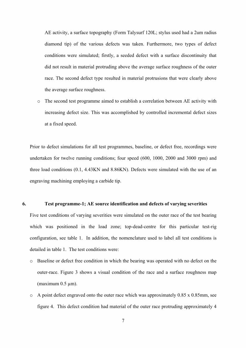
AE activity, a surface topography (Form Talysurf 120L; stylus used had a 2um radius

diamond tip) of the various defects was taken. Furthermore, two types of defect

conditions were simulated; firstly, a seeded defect with a surface discontinuity that

did not result in material protruding above the average surface roughness of the outer

race. The second defect type resulted in material protrusions that were clearly above

the average surface roughness.

o The second test programme aimed to establish a correlation between AE activity with

increasing defect size. This was accomplished by controlled incremental defect sizes

at a fixed speed.

Prior to defect simulations for all test programmes, baseline, or defect free, recordings were

undertaken for twelve running conditions; four speed (600, 1000, 2000 and 3000 rpm) and

three load conditions (0.1, 4.43KN and 8.86KN). Defects were simulated with the use of an

engraving machining employing a carbide tip.

6. Test programme-1; AE source identification and defects of varying severities

Five test conditions of varying severities were simulated on the outer race of the test bearing

which was positioned in the load zone; top-dead-centre for this particular test-rig

configuration, see table 1. In addition, the nomenclature used to label all test conditions is

detailed in table 1. The test conditions were:

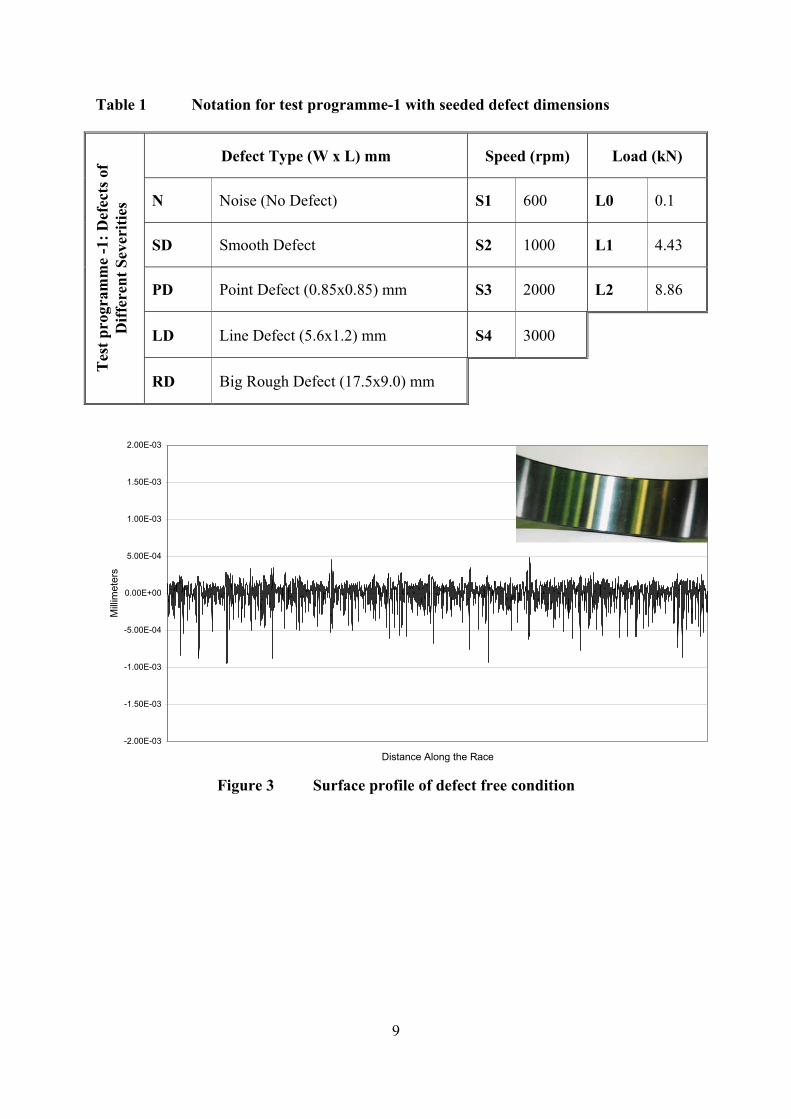
o Baseline or defect free condition in which the bearing was operated with no defect on the

outer-race. Figure 3 shows a visual condition of the race and a surface roughness map

(maximum 0.5 µm).

o A point defect engraved onto the outer race which was approximately 0.85 x 0.85mm, see

figure 4. This defect condition had material of the outer race protruding approximately 4

8

µm above the bearing maximum surface roughness.

o A line defect, approximately 5.6 x 1.2 mm, see figure 5.

o A rough defect, approximately 17.5 x 9.0 mm, see figure 6.

o A smooth defect in which a surface discontinuity, not influencing the average surface

roughness, was simulated. In this particular instance a grease hole on the outer race

matched the requirements, see figure 7. From figure 7 it is evident that the point of

discontinuity of the surface does not have a protrusion above the surface roughness as

evident for the ‘point’ or ‘line’ defect conditions. The main purpose of this simulation is

to observe if any changes in the load distribution will lead to generation or changes in AE

activity in comparison to a defect free condition.

All defects were run under four speeds (600, 1000, 2000 and 3000 rpm) and three different

loads (0.1, 4.43 and 8.86 KN). It must be noted that the defect length is along the race in the

direction of the rolling action and the defect width is across the race.

9

Table 1 Notation for test programme-1 with seeded defect dimensions

Defect Type (W x L) mm Speed (rpm) Load (kN)

N Noise (No Defect) S1 600 L0 0.1

SD Smooth Defect S2 1000 L1 4.43

PD Point Defect (0.85x0.85) mm S3 2000 L2 8.86

LD Line Defect (5.6x1.2) mm S4 3000

Tes

t pro

gram

me

-1: D

efec

ts o

f D

iffer

ent S

ever

ities

RD Big Rough Defect (17.5x9.0) mm

-2.00E-03

-1.50E-03

-1.00E-03

-5.00E-04

0.00E+00

5.00E-04

1.00E-03

1.50E-03

2.00E-03

Distance Along the Race

Milli

met

ers

Figure 3 Surface profile of defect free condition

10

-4.00E-03

-3.00E-03

-2.00E-03

-1.00E-03

0.00E+00

1.00E-03

2.00E-03

3.00E-03

4.00E-03

5.00E-03


Milli

met

er

0.85 mm

Figure 4 Surface profile of point defect condition

-2.50E-03

-2.00E-03

-1.50E-03

-1.00E-03

-5.00E-04

0.00E+00

5.00E-04

1.00E-03

1.50E-03

2.00E-03


Milli

met

ers

1.2 mm

Figure 5 Surface profile of a line defect condition

11

Figure 6 Rough defect condition

-1.00E-02

-8.00E-03

-6.00E-03

-4.00E-03

-2.00E-03

0.00E+00

2.00E-03

4.00E-03

6.00E-03


Milli

met

er

Defect (Hole) Starts Here

Edge of Defect is Smooth

Figure 7 Surface profile of a smooth defect condition

12

7. Test programme-2; Defects of varying size

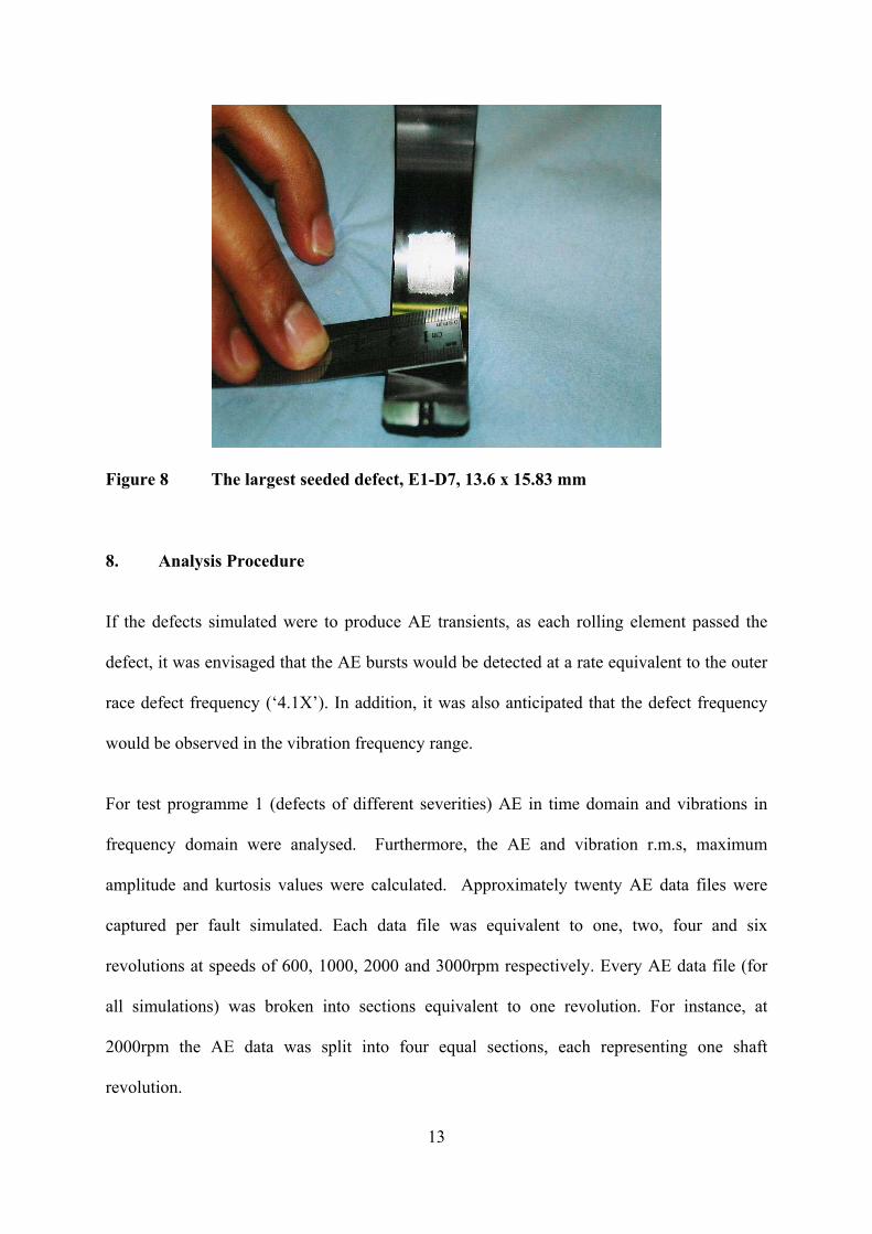
For this particular test programme, two experiments (E1 and E2) were carried out to

authenticate observations relating AE to varying defect sizes. Each experiment included

seven defects of different lengths and widths, see table 2. A sample defect is shown in figure

8. In experiment-1 (E1), a point defect (D1) was increased in length in three steps (D2 to D4)

and then increased in width in three more steps (D5 to D7). However, in experiment-2 (E2),

a point defect was increased in width and then in length interchangeably from D1 to D7.

Both experiments were run at 2000 rpm and at a load of 4.4kN. The AE sampling rates for

the first and second experiments are 8MHz and 10 MHz respectively. In experiment-2,

vibration was acquired in addition to AE for comparative purposes.

Table 2 Notation for test programme-2 with seeded defect dimensions

Experiment 1 Experiment 2

Defect Size, (width x length) mm Defect Size, (width x length) mm

E1-D0 No defect E2-D0 No defect

E1-D1 0.85 x 0.85 mm E2-D1 0.85 x 1.35 mm

E1-D2 1 x 2.95 mm E2-D2 2. x 1.35 mm

E1-D3 1 x 7.12 mm E2-D3 2 x 4 mm

E1-D4 1 x 15.83 mm E2-D4 4 x 4 mm

E1-D5 3.98 x 15.83 mm E2-D5 8 x 4 mm

E1-D6 8.66 x 15.83 mm E2-D6 13 x 4 mm

Tes

t Pro

gram

me

2: D

efec

ts o

f Diff

eren

t Siz

es

E1-D7 13.6 x 15.83 mm E2-D7 13x 10 mm

13

Figure 8 The largest seeded defect, E1-D7, 13.6 x 15.83 mm

8. Analysis Procedure

If the defects simulated were to produce AE transients, as each rolling element passed the

defect, it was envisaged that the AE bursts would be detected at a rate equivalent to the outer

race defect frequency (‘4.1X’). In addition, it was also anticipated that the defect frequency

would be observed in the vibration frequency range.

For test programme 1 (defects of different severities) AE in time domain and vibrations in

frequency domain were analysed. Furthermore, the AE and vibration r.m.s, maximum

amplitude and kurtosis values were calculated. Approximately twenty AE data files were

captured per fault simulated. Each data file was equivalent to one, two, four and six

revolutions at speeds of 600, 1000, 2000 and 3000rpm respectively. Every AE data file (for

all simulations) was broken into sections equivalent to one revolution. For instance, at

2000rpm the AE data was split into four equal sections, each representing one shaft

revolution.

14

The diagnostic parameters of r.m.s, etc, were calculated for each shaft revolution and

averaged for all data files. This implied that at 2000rpm, and for twenty data files, a total of

eighty AE r.m.s values were calculated and the value presented is the average of the eight

values. For vibration analysis, two data files were acquired for each simulation. This was

equivalent to 50, 83, 166 and 250 revolutions per data file at speeds of 600, 1000, 2000 and

3000rpm respectively. The exact procedure for calculating the AE parameters was employed

on the vibration data.

For test programme-2 observations of AE burst duration, r.m.s and amplitude for the various

defect sizes were undertaken. The burst duration was obtained by calculating the duration

from the point at which the AE response was higher than the underlying background noise

level to the point at which it returned to the underlying noise level. This procedure was

undertaken for every data file and the average value for each simulated case is presented.

9. Data Analysis; Test Programme-1

9.1 Observations of AE time waveform

As already stated the outer race defect frequency was calculated for the various test speeds;

41, 69, 137 and 205Hz at 600, 1000, 2000 and 3000rpm respectively. Typical AE and

vibration time waveforms for two different conditions are displayed in figures 9 and 10. It

was noted that for all defects conditions, other than the smooth defect, AE burst activity was

noted at the outer race defect frequency. Observations of AE time waveforms from noise and

smooth defect conditions showed random AE bursts that occurred at a rate which could not

be related to any machine phenomenon. Correspondingly, such transient bursts associated

with the presence of the defect were not observed on vibration waveforms, but more

15

interestingly, the outer race defect frequency was not observed on the frequency spectra of

most vibration data, except at one defect condition; rough defect, 3000rpm, load 0.1KN, see

figure 11.

Figure 9 AE time waveforms for all defects at a speed of 1000 rpm and a load 4.43kN

N SD PD LD RD

16

Figure 10 Vibration time waveforms for all defects at a speed of 1000 rpm and a load 4.43kN

N SD PD LD RD

17

Figure 11 Sample vibration data in the frequency domain

BPO = 205 Hz S4-L0-RD

S3-L1-RD

S2-L2-RD

S1-L1-RD

18

9.2 Observations of r.m.s values

The r.m.s values of AE and vibration signatures for all defect and defect free conditions were

compared for increasing speeds, see figures 12 and 13. For all test conditions, the AE r.m.s

value increased with increasing the speed at a fixed load. It was also noted that the AE r.m.s

values of noise and smooth defect were similar while AE r.m.s values increased with

increased defect severity; point, line and rough defects respectively. For a fixed speed and

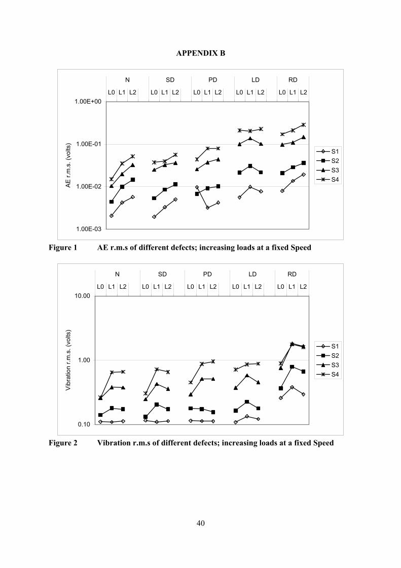
variable load it was observed that in general AE r.m.s increased with load, which increased

also with increasing defect severity, see figure 1 of appendix B. The vibration r.m.s values

showed a relatively small increase with increasing defect size, however, a clear increase in

vibration r.m.s was observed for the rough defect, see figure 13. Table 1 in appendix A

highlights the percentage change of r.m.s values for different defect sizes, emphasising the

sensitivity of AE to defect size progression, see figures 14 and 15. The percentage values

presented in Appendix A and figures 14 and 15 were obtained by relating all speed and load

defect simulations to the corresponding speed and load condition for the defect free (noise)

simulation. Figures 1 and 2 of appendix B show the vibration and AE r.m.s values for

increasing loads at fixed speeds.

19

1.00E-03

1.00E-02

1.00E-01

1.00E+00S1 S2 S3 S4 S1 S2 S3 S4 S1 S2 S3 S4 S1 S2 S3 S4 S1 S2 S3 S4

N SD PD LD RDA

E r.

m.s

. (vo

lts)

L0

L1

L2

Figure 12 AE r.m.s of different defects; increasing speeds at a fixed Load

0.10

1.00

10.00S1 S2 S3 S4 S1 S2 S3 S4 S1 S2 S3 S4 S1 S2 S3 S4 S1 S2 S3 S4

N SD PD LD RD

Vib

ratio

n r.m

.s. (

volts

)

L0L1L2

Figure 13 Vibration r.m.s of different defects; increasing speeds at a fixed Load

20

-40%

160%

360%

560%

760%

960%

1160%

1360%

S1 S2 S3 S4 S1 S2 S3 S4 S1 S2 S3 S4 S1 S2 S3 S4 S1 S2 S3 S4

N SD PD LD RD

% c

hang

e re

lativ

e to

def

ect f

ree

cond

ition

L0L1L2

Figure 14 Percentage change in AE r.m.s

-10%

40%

90%

140%

190%

240%

290%

340%

390%

440%

S1 S2 S3 S4 S1 S2 S3 S4 S1 S2 S3 S4 S1 S2 S3 S4 S1 S2 S3 S4

N SD PD LD RD

% c

hang

e re

lativ

e to

def

ect f

ree

cond

ition

L0L1L2

Figure 15 Percentage change in vibration r.m.s

21

9.3 Observations of maximum amplitude

It was noted that AE max amplitude increased with increasing speed for a fixed load, see

figure 16. Also it was evident that as the defect size was increased, the maximum AE

amplitude increased. The maximum AE amplitude increased from noise condition to the

point defect and increased further for the line defect. The maximum amplitude for the rough

defect was comparable to the ‘line’ defect. Again it was noted that values for ‘noise’ and

‘smooth’ conditions were similar. Vibration amplitude values were similar for all defect

conditions except for the rough defect, see figure 17. Table 2 in appendix A highlights the

percentage changes of maximum amplitude values for different defect sizes. These were

determined as detailed in the previous section. Figures 3 and 4 of Appendix B show the

vibration and AE maximum amplitude values for increasing loads at fixed speeds.

22

0.01

0.10

1.00


N SD PD LD RDA

E M

axim

um A

mpl

itude

(vol

ts)

L0L1L2

Figure 16 AE max amplitude of different defects at increasing speeds and fixed load

0.10

1.00


N SD PD LD RD

Vib

ratio

n M

ax A

mpl

itude

(vol

ts)

L0L1L2

Figure 17 Vibration max amplitude of different defects at increasing speeds and

fixed load

23

9.4 Observations of Kurtosis

Kurtosis is a measure of the peakness of a distribution and is widely established as a good

indicator of bearing health for vibration analysis. For a normal distribution, kurtosis is equal

to 3. The AE kurtosis values for the noise signal (N) and the smooth defect (SD) were

approximately ‘3’, see figure 18, as expected for a random distribution. It was noted that as

defect size increased from ‘noise’ to ‘point’ to ‘line’, the kurtosis values increased

accordingly. For the worst defect condition it was observed that the kurtosis values were

lower than for the preceding defect condition (line defect). This was not unexpected because

as the defect condition worsens it is known that kurtosis values will decrease; figure 18

depicts this observation. Kurtosis results for vibration showed similar values for all defect

simulations apart from the rough defect where a relative increase was noted, see figure 19

Table 3 in appendix A highlights the change of kurtosis values for different defect sizes,

emphasising the sensitivity of AE to defect size progression. Figures 5 and 6 of Appendix B

show the vibration and AE kurtosis values for increasing loads at fixed speeds.

24

1.00E+00

1.00E+01

1.00E+02

1.00E+03S1 S2 S3 S4 S1 S2 S3 S4 S1 S2 S3 S4 S1 S2 S3 S4 S1 S2 S3 S4

N SD PD LD RDA

E K

urto

sis

Val

ue

L 0L 2L 5

Figure 18 AE kurtosis of different defects at increasing speeds and fixed load

1.00

10.00


N SD PD LD RD

Vib

ratio

n K

urto

sis

Val

ue

L0L1L2

Figure 19 Vibration kurtosis of different defects at increasing speeds and fixed load

25

10. Data analysis: Test programme-2

The analysis of this test program was centered on AE time domain observations.

10.1. Observations of experiment-1 (E1)

This experiment included seven defect conditions; D1 to D4 had a fixed width with

increasing length while defects D4 to D7 had a fixed length with increasing width; see table

2. From observations of the AE time waveforms, AE bursts were clearly evident from defects

D4 to D7, see figure 20. The x-axis in these figures corresponds to one shaft revolution at

2000rpm. For defects D4 to D7 the width of associated defect AE burst was measured in an

attempt to relate the AE burst duration to the defect size. Interestingly, the bursts with equal

defect length D4 to D7 had near identical burst durations, see figure 21. For the other defects

(D1 to D3), the burst duration could not be separated from underlying background noise,

most probably due to the size of the seeded defect. Also it was observed that the ratio of

amplitude of the AE burst to underlying operational background noise increased

incrementally from D4 through to D7, as the defect increased in width, see table 3.

Table 3 Burst to noise ratio’s for defects of fixed defect length (15.8mm)

Defect Burst duration (second)

Burst amplitude (volt)

Noise amplitude(volt)

Burst to noise ratio

D4 0.0061 0.13 0.09 1.4:1 D5 0.0056 0.18 0.09 2.0:1 D6 0.0056 0.33 0.11 3.0:1 D7 0.0056 0.46 0.10 4.6:1

Two conclusions can be drawn, firstly, increasing the defect width increased the ratio of burst

amplitude to operational noise (i.e., the burst signal was increasingly more evident above the

operational noise levels, see figure 20). Secondly, it was deduced that increasing the defect

length increased the burst duration. To confirm this, a second experiment was performed

utilizing the same running conditions but with different defect size combinations.

26

Furthermore, the second test was undertaken to ensure repeatability, and a new bearing of

identical type to that used in experiment-1 was employed.

Figure 20 Sample AE time wave forms for defects D0 to D7 (Experiment-1)

D0 D1 D2 D3 D4 D5 D6 D7

27

Figure 21 Burst duration for defect D6 & D7 (Experiment-1)

10.2. Observations of experiment 2 (E2):

The difference between this experiment and that reported in the previous section is two fold.

Firstly, the defect size and arrangement of the seeded defect progression was different from

experiment-1 and secondly, the AE data captured was sampled at 10 MHz.

Observations of the bursts durations for defects D1 to D7, see figure 22, identified that for

defects D3 to D7, the burst duration was discernable; these defects had widths of at least 2

mm. It was also observed that the AE bursts for defects D3 to D6 (figure 23) were similar;

these defects had the same length of 4 mm. Clearly when the defect was increased in length

from 4mm to 10mm (D6 to D7) the burst duration increased dramatically, see figures 23 and

24.

0.0056 s

0.0056 s

0.0056 s

28

Table 4 Burst to noise ratio’s for defects with a fixed length (4mm) and a defect (D7) with an increased length (10mm)

Defect Burst duration (second)

Burst amplitude (volt)

Noise amplitude(volt)

Signal to noise ratio

D3 0.0018 0.17 0.10 1.7:1 D4 0.0018 0.24 0.09 2.7:1 D5 0.0019 0.32 0.10 3.2:1 D6 0.0019 0.43 0.11 3.9:1 D7 0.0036 0.42 0.11 3.8:1

29

Figure 22 Sample AE time wave-forms for defects D0 to D7 (Experiment-2)

D0 D1 D2 D3 D4 D5 D6 D7

30

Figure 23 AE waveform bursts for defects D5-D6 (Experiment-2)

Figure 24 AE waveform burst for defect D7 (Experiment-2)

A summary of AE burst duration for experiments-1 and -2 are detailed in table 5. From table

5 a linear relation between the burst duration and the defect length is observed, see figure 25.

The variation of this data about the mean was approximately ± 10%.

0.0036 s

0.0019 s

0.0019 s

31

Table 5 Defect length and width vs. burst duration from experiments 1 and 2

Exp. Defect Length in mm Width in mm Burst Duration in seconds

2 D3 to D6 4 4, 8 and 13 0.00185

2 D7 10 13 0.00360

1 D5 to D7 15.83 4, 9 and 14 0.00564

AE Burst Duration vs. Defect Length

0

2

4

6

8

10

12

14

16

18

0.00185 0.00360 0.00564

Burst Duration

Def

ect L

engt

h in

mm

Figure 25 AE burst duration vs. defect length

Observations of vibration measurements in experiment-2 of test programme 2 failed to locate

the defect source under all simulations but one condition, D3-L1. This was in contrast to AE.

The r.m.s and maximum amplitude values for AE and vibrations obtained in test programme-

2, experiment-2, are detailed in figures 26 and 27. These were calculated per data file. Again

as reported in test programme-1, AE r.m.s increased from defect size ‘D1’ onwards whilst

AE maximum amplitude values increased from defect size ‘D3’, see figure 26 and 27. In

contrast vibration r.m.s and maximum amplitude values have increased for defects D4

onwards, see figures 26 and 27.

Variation ± 10%

32

0

0.5

1

1.5

2

2.5

3

D1 D2 D3 D4 D5 D6 D7

Defect

Vib

ratio

n M

ax. A

mpl

itude

(Vol

ts)

0.00E+00

1.00E-01

2.00E-01

3.00E-01

4.00E-01

5.00E-01

6.00E-01

7.00E-01

AE

Max

. Am

plitu

de (V

olts

)

VibrationAE

Figure 26 AE maximum amplitude values for experiment-2, defects D1 to D7

0

0.2

0.4

0.6

0.8

1

1.2

D1 D2 D3 D4 D5 D6 D7

Defect

Vib

ratio

n R

MS

(Vol

ts)

0.00E+00

2.00E-02

4.00E-02

6.00E-02

8.00E-02

1.00E-01

1.20E-01

AE

RM

S (V

olts

)

VibrationAE

Figure 27 Vibration r.m.s values for experiment-2, defects D1 to D7

33

11. Discussions

The source of AE for seeded defects is attributed to material protrusions above the surface

roughness of the outer race. This was established as the smooth defect could not be

distinguished from the no-defect condition. However, for all other defects where the material

protruded above the surface roughness, AE transients associated with the defect frequency

were observed. As the defect size increased, AE r.m.s, maximum amplitude and kurtosis

values increased, however, observations of corresponding parameters from vibration

measurements were disappointing. Although the vibration r.m.s and maximum amplitude

values did show changes with defect condition, the rate of such changes highlighted the

greater sensitivity of the AE technique to early defect detection, see appendix A. Again,

unlike vibration measurements, the AE transient bursts could be related to the defect source

whilst the frequency spectrum of vibration readings failed in the majority of cases to identify

the defect frequency or source. Also evident from this investigation is that AE levels increase

with increasing speed and load. It should be noted that further signal processing could be

applied to the vibration data in an attempt to enhance defect detection. Techniques such as

demodulation, band pass filtering, etc, could be applied though these were not employed for

this particular investigation. The main reason for not applying further signal processing to the

vibration data was to allow a direct comparison between the acquired AE and vibration

signature. From the results presented two important features were noted; firstly, AE was more

sensitive than vibration to variation in defect size, and secondly, that no further analysis of

the AE response was required in relating the defect source to the AE response, which was not

the case for vibration signatures.

The relationship between defect size and AE burst duration is a significant finding. In the

34

longer term, and with further research, this offers opportunities for prognosis. AE burst

duration was directly correlated to the seeded defect length (along the race in the direction of

the rolling action) whilst the ratio of burst amplitude to the underlying operational noise

levels was directly proportional to the seeded defect width.

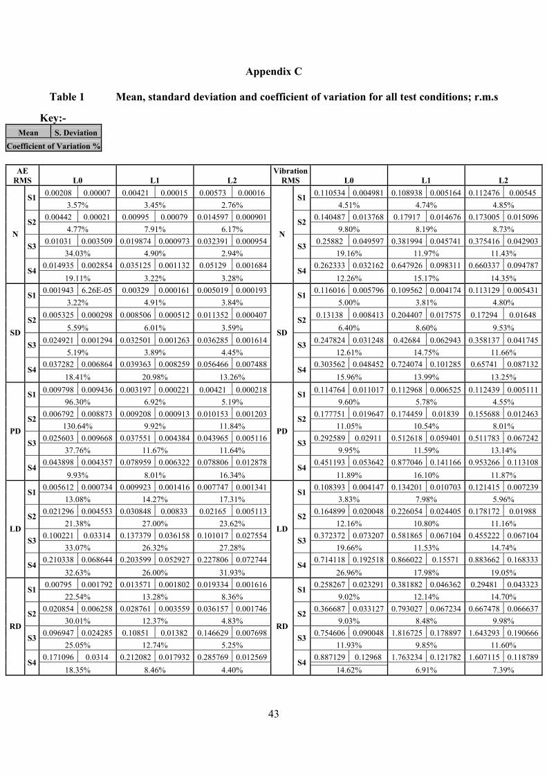
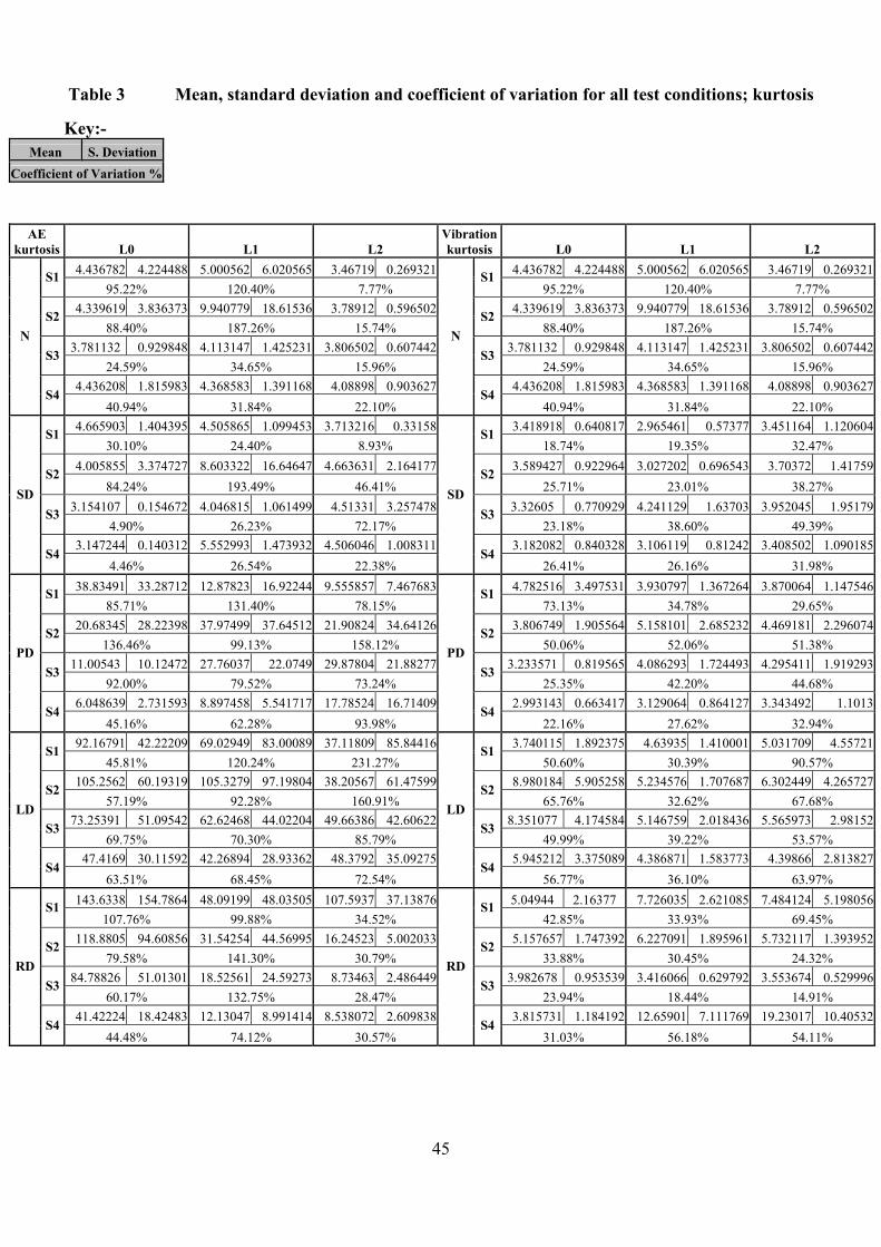
The variation of all data presented for test programme’s 1 and 2 are detailed in tables 1 to 3 in

Appendix C and tables 1 to 4 in appendix D. The standard deviation and coefficient of

variation (CV) for all parameters presented in the paper are detailed. The CV is a measure of

the relative dispersion in a set of measurements. From appendix C it was noted that the

average CV for r.m.s, maximum amplitude and kurtosis for AE was 17%, 43% and 73%

respectively. Correspondingly the average CV for equivalent vibration parameters was 11%,

26% and 43%. This showed that the kurtosis measurements/calculations had a greater

variability about the average value than r.m.s and maximum amplitude. For test programme-2

the CV was less than 20% for AE parameters and just over 30% for vibration parameters.

12 Conclusion

It has been shown that the fundamental source of AE in seeded defect tests was due to

material protrusions above the mean surface roughness. Also, AE r.m.s, maximum amplitude

and kurtosis have all been shown to be more sensitive to the onset and growth of defects than

vibration measurements. A relationship between the AE burst duration and the defect length

has been presented.

35

13. References

1. Mathews, J. R. Acoustic emission, Gordon and Breach Science Publishers Inc., New

York. 1983, ISSN 0730-7152.

2. Roger, L. M., The application of vibration analysis and acoustic emission source

location to on-line condition monitoring of anti-friction bearings. Tribology International,

1979; 51-59.

3. Mba, D., Bannister, R.H., and Findlay, G.E. Condition monitoring of low-speed

rotating machinery using stress waves: Part’s I and II. Proceedings of the Instn Mech Engr

1999; 213(E): 153-185

4. N. Jamaludin, Dr. D. Mba, Dr. R. H. Bannister Condition monitoring of slow-speed

rolling element bearings using stress waves. Journal of Process Mechanical Engineering, I

Mech E. Pro. Inst. Mech Eng., 2001, 215(E):, Issue E4, 245-271.

5. Yoshioka T, Fujiwara T. New acoustic emission source locating system for the study

of rolling contact fatigue, Wear, 81(1), 183-186.

6. Yoshioka T, Fujiwara T. Application of acoustic emission technique to detection of

rolling bearing failure, American Society of Mechanical Engineers, Production Engineering

Division publication PED, 1984, 14, 55-76.

7. Hawman, M. W., Galinaitis, W. S, Acoustic Emission monitoring of rolling element

bearings, Proceedings of the IEEE, Ultrasonics symposium, 1988, 885-889

8. Holroyd, T.J. and Randall, N., (1993), Use of Acoustic Emission for Machine

Condition Monitoring, British Journal of Non-Destructive Testing, 1993, 35(2), 75-78.

9. Holroyd, T. Condition monitoring of very slowly rotating machinery using AE

techniques. 14th International congress on Condition monitoring and Diagnostic engineering

management (COMADEM'2001), Manchester, UK, 4-6 September 2001, 29, ISBN

36

0080440363

10. Bagnoli, S., Capitani, R. and Citti, P. Comparison of accelerometer and acoustic

emission signals as diagnostic tools in assessing bearing. Proceedings of 2nd International

Conference on Condition Monitoring, London, UK, May 1988, 117-125.

11. Morhain, A, Mba, D, Bearing defect diagnosis and acoustic emission Journal of

Engineering Tribology, I Mech E, Vol 217, No. 4, Part J, p 257-272, 2003. ISSN 1350-

6501.

12. Mathews, J. R. Acoustic emission, Gordon and Breach Science Publishers Inc., New

York. 1983, ISSN 0730-7152

13. Tan, C.C. Application of acoustic emission to the detection of bearing failures. The

Institution of Engineers Australia, Tribology conference, Brisbane, 3-5 December 1990, 110-

114.

37

APPENDIX A

Table 1 Percentage changes in vibration and AE r.m.s values

AE % Change L0 L1 L2 VIB % Change L0 L1 L2

S1 0% 0% 0% S1 0% 0% 0%

S2 0% 0% 0% S2 0% 0% 0%

S3 0% 0% 0% S3 0% 0% 0% N

S4 0% 0% 0%

N

S4 0% 0% 0%

S1 -6% -22% -13% S1 5% 1% 1%

S2 20% -15% -22% S2 -6% 14% 0%

S3 141% 63% 12% S3 -4% 12% -5% SD

S4 150% 12% 10%

SD

S4 16% 12% 0%

S1 371% -24% -27% S1 4% 4% 0%

S2 54% -7% -30% S2 27% -3% -10%

S3 148% 89% 36% S3 13% 34% 36% PD

S4 194% 124% 54%

PD

S4 72% 35% 44%

S1 170% 135% 35% S1 -2% 23% 8%

S2 383% 210% 49% S2 17% 26% 3%

S3 871% 590% 212% S3 44% 52% 21% LD

S4 1313% 479% 344%

LD

S4 172% 34% 34%

S1 284% 223% 237% S1 134% 251% 162%

S2 371% 189% 147% S2 161% 343% 286%

S3 843% 446% 353% S3 192% 376% 339% RD

S4 1048% 504% 458%

RD

S4 238% 172% 143%

38

Table 2 Percentage changes in AE and vibration maximum amplitude values


S1 0% 0% 0% S1 0% 0% 0%

S2 0% 0% 0% S2 0% 0% 0%

S3 0% 0% 0% S3 0% 0% 0% N

S4 0% 0% 0%

N

S4 0% 0% 0%

S1 13% -23% -20% S1 -3% -16% -5%

S2 11% -17% -9% S2 -6% 3% -6%

S3 90% 61% 12% S3 -10% 17% -8% SD

S4 75% 19% 10%

SD

S4 9% 22% 5%

S1 992% 23% 41% S1 -4% -8% -3%

S2 242% 72% 41% S2 16% 4% -11%

S3 347% 319% 199% S3 9% 30% 27% PD

S4 262% 205% 172%

PD

S4 71% 37% 40%

S1 918% 539% 262% S1 -21% 27% 7%

S2 1726% 664% 275% S2 39% 37% 10%

S3 3250% 1839% 692% S3 89% 67% 30% LD

S4 3546% 1264% 1026%

LD

S4 159% 44% 34%

S1 1652% 732% 1250% S1 110% 302% 186%

S2 1951% 376% 378% S2 147% 330% 301%

S3 3681% 883% 482% S3 209% 288% 260% RD

S4 2992% 754% 579%

RD

S4 264% 155% 115%

39

Table 3 Percentage changes in vibration and AE kurtosis values


S1 0% 0% 0% S1 0% 0% 0%

S2 0% 0% 0% S2 0% 0% 0%

S3 0% 0% 0% S3 0% 0% 0% N

S4 0% 0% 0%

N

S4 0% 0% 0%

S1 6% -10% 7% S1 -16% -29% -18%

S2 -8% -14% 23% S2 -3% -17% -7%

S3 -16% -1% 19% S3 9% -7% -22% SD

S4 -29% 27% 10%

SD

S4 4% -11% -18%

S1 750% 158% 174% S1 18% -6% -8%

S2 328% 270% 479% S2 3% 42% 12%

S3 190% 575% 664% S3 6% -10% -15% PD

S4 37% 98% 336%

PD

S4 -2% -11% -20%

S1 1999% 1291% 965% S1 -8% 11% 20%

S2 2303% 932% 916% S2 142% 44% 57%

S3 1839% 1418% 1201% S3 175% 13% 10% LD

S4 974% 861% 1073%

LD

S4 95% 25% 6%

S1 3112% 864% 2995% S1 24% 84% 78%

S2 2637% 213% 328% S2 39% 71% 43%

S3 2136% 352% 129% S3 31% -25% -30% RD

S4 837% 178% 109%

RD

S4 25% 262% 363%

40

APPENDIX B

1.00E-03

1.00E-02

1.00E-01

1.00E+00L0 L1 L2 L0 L1 L2 L0 L1 L2 L0 L1 L2 L0 L1 L2

N SD PD LD RD

AE

r.m

.s. (

volts

)

S1S2S3S4

Figure 1 AE r.m.s of different defects; increasing loads at a fixed Speed

0.10

1.00

10.00L0 L1 L2 L0 L1 L2 L0 L1 L2 L0 L1 L2 L0 L1 L2

N SD PD LD RD

Vib

ratio

n r.m

.s. (

volts

)

S1S2S3S4

Figure 2 Vibration r.m.s of different defects; increasing loads at a fixed Speed

41

0.01

0.10

1.00


N SD PD LD RDA

E M

axim

um A

mpl

itude

(vol

ts)

S1S2S3S4

Figure 3 AE max amplitude of different defects at increasing loads and fixed speed

fixed load

0.10

1.00


N SD PD LD RD

Vib

ratio

n M

ax A

mpl

itude

(vol

ts)

S1S2S3S4

Figure 4 Vibration max amplitude of different defects at increasing loads and fixed

speed

42

1.00E+00

1.00E+01

1.00E+02

1.00E+03L0 L1 L2 L0 L1 L2 L0 L1 L2 L0 L1 L2 L0 L1 L2

N SD PD LD RD

AE

Kur

tosi

s V

alue

S6S1S2S3

Figure 5 AE kurtosis of different defects at increasing loads and fixed speed

1.00

10.00


N SD PD LD RD

Vib

ratio

n K

urto

sis

Val

ue

S1S2S3S4

Figure 6 Vibration kurtosis of different defects at increasing loads and fixed speed

43

Appendix C

Table 1 Mean, standard deviation and coefficient of variation for all test conditions; r.m.s Key:-

Mean S. Deviation Coefficient of Variation %

AE RMS L0 L1 L2

Vibration RMS L0 L1 L2

0.00208 0.00007 0.00421 0.00015 0.00573 0.00016 0.110534 0.004981 0.108938 0.005164 0.112476 0.00545 S1 3.57% 3.45% 2.76%

S14.51% 4.74% 4.85%

0.00442 0.00021 0.00995 0.00079 0.014597 0.000901 0.140487 0.013768 0.17917 0.014676 0.173005 0.015096S2 4.77% 7.91% 6.17%

S29.80% 8.19% 8.73%

0.01031 0.003509 0.019874 0.000973 0.032391 0.000954 0.25882 0.049597 0.381994 0.045741 0.375416 0.042903S3 34.03% 4.90% 2.94%

S319.16% 11.97% 11.43%

0.014935 0.002854 0.035125 0.001132 0.05129 0.001684 0.262333 0.032162 0.647926 0.098311 0.660337 0.094787

N

S4 19.11% 3.22% 3.28%

N

S412.26% 15.17% 14.35%

0.001943 6.26E-05 0.00329 0.000161 0.005019 0.000193 0.116016 0.005796 0.109562 0.004174 0.113129 0.005431S1 3.22% 4.91% 3.84%

S15.00% 3.81% 4.80%

0.005325 0.000298 0.008506 0.000512 0.011352 0.000407 0.13138 0.008413 0.204407 0.017575 0.17294 0.01648 S2 5.59% 6.01% 3.59%

S26.40% 8.60% 9.53%

0.024921 0.001294 0.032501 0.001263 0.036285 0.001614 0.247824 0.031248 0.42684 0.062943 0.358137 0.041745S3 5.19% 3.89% 4.45%

S312.61% 14.75% 11.66%

0.037282 0.006864 0.039363 0.008259 0.056466 0.007488 0.303562 0.048452 0.724074 0.101285 0.65741 0.087132

SD

S4 18.41% 20.98% 13.26%

SD

S415.96% 13.99% 13.25%

0.009798 0.009436 0.003197 0.000221 0.00421 0.000218 0.114764 0.011017 0.112968 0.006525 0.112439 0.005111S1 96.30% 6.92% 5.19%

S19.60% 5.78% 4.55%

0.006792 0.008873 0.009208 0.000913 0.010153 0.001203 0.177751 0.019647 0.174459 0.01839 0.155688 0.012463S2 130.64% 9.92% 11.84%

S211.05% 10.54% 8.01%

0.025603 0.009668 0.037551 0.004384 0.043965 0.005116 0.292589 0.02911 0.512618 0.059401 0.511783 0.067242S3 37.76% 11.67% 11.64%

S39.95% 11.59% 13.14%

0.043898 0.004357 0.078959 0.006322 0.078806 0.012878 0.451193 0.053642 0.877046 0.141166 0.953266 0.113108

PD

S4 9.93% 8.01% 16.34%

PD

S411.89% 16.10% 11.87%

0.005612 0.000734 0.009923 0.001416 0.007747 0.001341 0.108393 0.004147 0.134201 0.010703 0.121415 0.007239S1 13.08% 14.27% 17.31%

S13.83% 7.98% 5.96%

0.021296 0.004553 0.030848 0.00833 0.02165 0.005113 0.164899 0.020048 0.226054 0.024405 0.178172 0.01988 S2 21.38% 27.00% 23.62%

S212.16% 10.80% 11.16%

0.100221 0.03314 0.137379 0.036158 0.101017 0.027554 0.372372 0.073207 0.581865 0.067104 0.455222 0.067104S3 33.07% 26.32% 27.28%

S319.66% 11.53% 14.74%

0.210338 0.068644 0.203599 0.052927 0.227806 0.072744 0.714118 0.192518 0.866022 0.15571 0.883662 0.168333

LD

S4 32.63% 26.00% 31.93%

LD

S426.96% 17.98% 19.05%

0.00795 0.001792 0.013571 0.001802 0.019334 0.001616 0.258267 0.023291 0.381882 0.046362 0.29481 0.043323S1 22.54% 13.28% 8.36%

S19.02% 12.14% 14.70%

0.020854 0.006258 0.028761 0.003559 0.036157 0.001746 0.366687 0.033127 0.793027 0.067234 0.667478 0.066637S2 30.01% 12.37% 4.83%

S29.03% 8.48% 9.98%

0.096947 0.024285 0.10851 0.01382 0.146629 0.007698 0.754606 0.090048 1.816725 0.178897 1.643293 0.190666S3 25.05% 12.74% 5.25%

S311.93% 9.85% 11.60%

0.171096 0.0314 0.212082 0.017932 0.285769 0.012569 0.887129 0.12968 1.763234 0.121782 1.607115 0.118789

RD

S4 18.35% 8.46% 4.40%

RD

S414.62% 6.91% 7.39%

44

Table 2 Mean, standard deviation and coefficient of variation for all test conditions; maximum amplitude Key:-


AE max. amplitud

e L0 L1 L2

Vibration max.

amplitude L0 L1 L2

0.0149 0.006524 0.036803 0.020128 0.04131 0.011605 0.426122 0.104572 0.37851 0.094475 0.376092 0.067449S1 43.78% 54.69% 28.09%

S124.54% 24.96% 17.93%

0.029569 0.013988 0.102148 0.065422 0.108597 0.027766 0.455451 0.114607 0.589201 0.141621 0.573061 0.156391S2 47.31% 64.05% 25.57%

S225.16% 24.04% 27.29%

0.060725 0.028089 0.13416 0.032667 0.221715 0.049594 0.684509 0.169395 1.065683 0.315576 1.121585 0.391334S3 46.26% 24.35% 22.37%

S324.75% 29.61% 34.89%

0.095059 0.031538 0.236697 0.0657 0.33793 0.076411 0.637855 0.123435 1.50238 0.400672 1.547755 0.49042

N

S4 33.18% 27.76% 22.61%

N

S419.35% 26.67% 31.69%

0.016767 0.00644 0.028275 0.00826 0.033363 0.006056 0.411469 0.075882 0.318643 0.066042 0.356 0.067684S1 38.41% 29.21% 18.15%

S118.44% 20.73% 19.01%

0.033616 0.013939 0.084782 0.051091 0.097653 0.032219 0.426683 0.086709 0.609701 0.124684 0.541524 0.108176S2 41.47% 60.26% 32.99%

S220.32% 20.45% 19.98%

0.115335 0.017671 0.215026 0.05394 0.250093 0.077732 0.614241 0.118372 1.25011 0.425267 1.027509 0.304789S3 15.32% 25.09% 31.08%

S319.27% 34.02% 29.66%

0.166421 0.032748 0.281803 0.06331 0.37256 0.068917 0.694292 0.149475 1.83638 0.487189 1.62518 0.456532

SD

S4 19.68% 22.47% 18.50%

SD

S421.53% 26.53% 28.09%

0.164954 0.158003 0.045307 0.018477 0.059005 0.023613 0.408531 0.120479 0.346724 0.071826 0.363265 0.071478S1 95.79% 40.78% 40.02%

S129.49% 20.72% 19.68%

0.105695 0.175902 0.177965 0.068597 0.15174 0.074084 0.528683 0.131054 0.615183 0.212818 0.511878 0.14524S2 166.42% 38.55% 48.82%

S224.79% 34.59% 28.37%

0.272127 0.180325 0.563662 0.21607 0.676773 0.238314 0.748415 0.126557 1.384229 0.411869 1.422985 0.472924S3 66.27% 38.33% 35.21%

S316.91% 29.75% 33.23%

0.343804 0.107785 0.727329 0.259129 0.922697 0.432785 1.089618 0.206767 2.060298 0.524359 2.166361 0.571468

PD

S4 31.35% 35.63% 46.90%

PD

S418.98% 25.45% 26.38%

0.15155 0.049152 0.23904 0.118443 0.150789 0.106757 0.335939 0.081127 0.482153 0.119156 0.40098 0.08549S1 32.43% 49.55% 70.80%

S124.15% 24.71% 21.32%

0.549966 0.203333 0.793367 0.444417 0.399768 0.2828 0.634 0.229519 0.806274 0.216681 0.631085 0.199209S2 36.97% 56.02% 70.74%

S236.20% 26.87% 31.57%

2.032534 1.121462 2.601124 1.308942 1.769984 0.93768 1.295439 0.578847 1.783113 0.575885 1.454256 0.551794S3 55.18% 50.32% 52.98%

S344.68% 32.30% 37.94%

3.45586 1.841971 3.23032 1.671089 3.833406 2.09603 1.650906 0.80296 2.166102 0.768099 2.077714 0.849431

LD

S4 53.30% 51.73% 54.68%

LD

S448.64% 35.46% 40.88%

0.262969 0.182349 0.306043 0.127173 0.564963 0.107298 0.893571 0.15583 1.522286 0.306173 1.075571 0.268539S1 69.34% 41.55% 18.99%

S117.44% 20.11% 24.97%

0.617684 0.409719 0.491357 0.291556 0.518636 0.109704 1.125646 0.211943 2.536524 0.415032 2.298293 0.471199S2 66.33% 59.34% 21.15%

S218.83% 16.36% 20.50%

2.302343 0.971546 1.321508 0.7621 1.296574 0.328188 2.114104 0.435389 4.138695 0.425519 4.035311 0.448041S3 42.20% 57.67% 25.31%

S320.59% 10.28% 11.10%

2.934978 0.938397 2.018096 0.734277 2.307621 0.481824 2.319563 0.585691 3.83158 0.688802 3.330045 1.508469

RD

S4 31.97% 36.38% 20.88%

RD

S425.25% 17.98% 45.30%

45

Table 3 Mean, standard deviation and coefficient of variation for all test conditions; kurtosis

Key:-


AE kurtosis L0 L1 L2

Vibration kurtosis L0 L1 L2

4.436782 4.224488 5.000562 6.020565 3.46719 0.269321 4.436782 4.224488 5.000562 6.020565 3.46719 0.269321S1 95.22% 120.40% 7.77%

S195.22% 120.40% 7.77%

4.339619 3.836373 9.940779 18.61536 3.78912 0.596502 4.339619 3.836373 9.940779 18.61536 3.78912 0.596502S2 88.40% 187.26% 15.74%

S288.40% 187.26% 15.74%

3.781132 0.929848 4.113147 1.425231 3.806502 0.607442 3.781132 0.929848 4.113147 1.425231 3.806502 0.607442S3 24.59% 34.65% 15.96%

S324.59% 34.65% 15.96%

4.436208 1.815983 4.368583 1.391168 4.08898 0.903627 4.436208 1.815983 4.368583 1.391168 4.08898 0.903627

N

S4 40.94% 31.84% 22.10%

N

S440.94% 31.84% 22.10%

4.665903 1.404395 4.505865 1.099453 3.713216 0.33158 3.418918 0.640817 2.965461 0.57377 3.451164 1.120604S1 30.10% 24.40% 8.93%

S118.74% 19.35% 32.47%

4.005855 3.374727 8.603322 16.64647 4.663631 2.164177 3.589427 0.922964 3.027202 0.696543 3.70372 1.41759S2 84.24% 193.49% 46.41%

S225.71% 23.01% 38.27%

3.154107 0.154672 4.046815 1.061499 4.51331 3.257478 3.32605 0.770929 4.241129 1.63703 3.952045 1.95179S3 4.90% 26.23% 72.17%

S323.18% 38.60% 49.39%

3.147244 0.140312 5.552993 1.473932 4.506046 1.008311 3.182082 0.840328 3.106119 0.81242 3.408502 1.090185

SD

S4 4.46% 26.54% 22.38%

SD

S426.41% 26.16% 31.98%

38.83491 33.28712 12.87823 16.92244 9.555857 7.467683 4.782516 3.497531 3.930797 1.367264 3.870064 1.147546S1 85.71% 131.40% 78.15%

S173.13% 34.78% 29.65%

20.68345 28.22398 37.97499 37.64512 21.90824 34.64126 3.806749 1.905564 5.158101 2.685232 4.469181 2.296074S2 136.46% 99.13% 158.12%

S250.06% 52.06% 51.38%

11.00543 10.12472 27.76037 22.0749 29.87804 21.88277 3.233571 0.819565 4.086293 1.724493 4.295411 1.919293S3 92.00% 79.52% 73.24%

S325.35% 42.20% 44.68%

6.048639 2.731593 8.897458 5.541717 17.78524 16.71409 2.993143 0.663417 3.129064 0.864127 3.343492 1.1013

PD

S4 45.16% 62.28% 93.98%

PD

S422.16% 27.62% 32.94%

92.16791 42.22209 69.02949 83.00089 37.11809 85.84416 3.740115 1.892375 4.63935 1.410001 5.031709 4.55721S1 45.81% 120.24% 231.27%

S150.60% 30.39% 90.57%

105.2562 60.19319 105.3279 97.19804 38.20567 61.47599 8.980184 5.905258 5.234576 1.707687 6.302449 4.265727S2 57.19% 92.28% 160.91%

S265.76% 32.62% 67.68%

73.25391 51.09542 62.62468 44.02204 49.66386 42.60622 8.351077 4.174584 5.146759 2.018436 5.565973 2.98152S3 69.75% 70.30% 85.79%

S349.99% 39.22% 53.57%

47.4169 30.11592 42.26894 28.93362 48.3792 35.09275 5.945212 3.375089 4.386871 1.583773 4.39866 2.813827

LD

S4 63.51% 68.45% 72.54%

LD

S456.77% 36.10% 63.97%

143.6338 154.7864 48.09199 48.03505 107.5937 37.13876 5.04944 2.16377 7.726035 2.621085 7.484124 5.198056S1 107.76% 99.88% 34.52%

S142.85% 33.93% 69.45%

118.8805 94.60856 31.54254 44.56995 16.24523 5.002033 5.157657 1.747392 6.227091 1.895961 5.732117 1.393952S2 79.58% 141.30% 30.79%

S233.88% 30.45% 24.32%

84.78826 51.01301 18.52561 24.59273 8.73463 2.486449 3.982678 0.953539 3.416066 0.629792 3.553674 0.529996S3 60.17% 132.75% 28.47%

S323.94% 18.44% 14.91%

41.42224 18.42483 12.13047 8.991414 8.538072 2.609838 3.815731 1.184192 12.65901 7.111769 19.23017 10.40532

RD

S4 44.48% 74.12% 30.57%

RD

S431.03% 56.18% 54.11%

46

Appendix D

Table 1 Mean, standard deviation and coefficient of variation for test programme-2; AE r.m.s

Average 0.03025 0.0339 0.03865 0.0479688 0.06255 0.0728235 0.0981857 Standard deviation 0.0005351 0.0008124 0.0012646 0.0028927 0.0030232 0.0038606 0.0036336 Coefficient of variation 1.77% 2.40% 3.27% 6.03% 4.83% 5.30% 3.70% Load 4.4kN D1 D2 D3 D4 D5 D6 D7

Table 2 Mean, standard deviation and coefficient of variation for test

programme-2; AE maximum amplitude

Average 0.2066417 0.1776417 0.2297167 0.3562063 0.4710313 0.549 0.6297857 Standard deviation 0.0398724 0.0306937 0.0412125 0.0253876 0.0503913 0.0670317 0.0736799 Coefficient of variation 19.30% 17.28% 17.94% 7.13% 10.70% 12.21% 11.70% Load 4.4kN D1 D2 D3 D4 D5 D6 D7


programme-2; Vibration r.m.s Average 0.429082 0.3148242 0.3610585 0.4984004 1.0070777 0.8177705 0.6699566 Standard deviation 0.0614877 0.0567484 0.0552029 0.0670442 0.137269 0.1381788 0.0760416 Coefficient of variation 14.33% 18.03% 15.29% 13.45% 13.63% 16.90% 11.35%

Load 4.4kN D1 D2 D3 D4 D5 D6 D7


programme-2; Vibration maximum amplitude Average 1.0728039 0.7673333 0.9027242 1.2201647 2.8411781 2.4977007 1.6514511 Standard deviation 0.3867745 0.2769304 0.3311302 0.3188992 0.7856587 0.8620226 0.4262681 Coefficient of variation 36.05% 36.09% 36.68% 26.14% 27.65% 34.51% 25.81%

Load 4.4kN D1 D2 D3 D4 D5 D6 D7

Documents

A comparative experimental study on the use of Acoustic