A COMPARATIVE STUDY OF FINITE ELEMENT METHODOLOGIES …

A COMPARATIVE STUDY OF FINITE

ELEMENT METHODOLOGIES FOR

TORSIONAL VIBRATION RESPONSE

CALCULATIONS OF BLADED ROTORS

by

Ronnie Scheepers

Submitted in fulfillment of part of the requirements for the degree of

Master of Engineering in the Faculty of Engineering, the Built

Environment and Information Technology

University of Pretoria

2013

©© UUnniivveerrssiittyy ooff PPrreettoorriiaa

i

A COMPARATIVE STUDY OF FINITE

ELEMENT METHODOLOGIES FOR

TORSIONAL VIBRATION RESPONSE

CALCULATIONS OF BLADED ROTORS

by

Ronnie Scheepers

Supervisor: Professor P.S. Heyns

Department of Mechanical and Aeronautical Engineering

Degree: M Eng

Summary

Turbo-generator trains are susceptible to torsional vibration which can lead to fatigue

cracking and failure. Methods are available for the measurement and calculation of the

torsional natural frequencies of these systems for the purpose of design, monitoring and

life prediction. Calculation methods are conventionally based on one dimensional (1D)

finite element (FE) methodologies which require the simplification of a number of aspects

including the participation of flexible blades in torsional vibration modes.

The accuracy of 1D, three dimensional (3D) and three dimensional cyclic symmetric

(3DCS) FE methods was investigated by the application thereof on a small test rotor.

Experimental measurements of static and dynamic vibration responses were conducted

with rotation and torsional forcing accomplished through the use of a DC motor and a

digital control system optimised for fast transient and stable steady state response. Blade

stagger angle was demonstrated to have a significant effect on torsional frequencies

although no stress stiffening effects were noted in the speed range considered. Similarly,

damping was measured to decrease with blade stagger angle but not with rotational speed.

Step changes in torsional frequencies due to the activation of the motor field and armature

currents required optimisation of the motor models for static and dynamic conditions.


ii

Shaft torsional vibration responses were found not to include all blade modes and vice

versa.

Full 3D parametric models with a high degree of geometric detail were generated and

meshed using commercial software ANSYS ver. 14.0. No simplification was introduced

other than for the armature motor where an equivalent material density and elastic

modulus was obtained by measurement and frequency calibration. Calculated torsional

frequencies agreed well with measured results for static and dynamic conditions. 3DCS

models obtained by simplification of the full 3D models resulted in similar accuracy but

lower solution times. Visualisation of torsional modes is enhanced by 3D modelling

which also includes rigid shaft modes which is not possible in the 1D approach.

Further reduction to 1D models requires a number of simplifications which result in

smaller models with low solution times but generally reduced accuracy. Blade torsional

participation was accomplished in the 1D approach using Euler-Bernoulli beam theory

and the component mode synthesis technique to calculate equivalent mass and stiffness as

well as the residual mass of each blade mode to be coupled. Simplifications for sudden

diameter changes and shrunk-on disks were also made.

It is concluded that all three FE techniques applied in this work are useful depending on

the required accuracy, available information and resources. In cases, where a high level of

accuracy is required, direct field measurements should be used for model calibration or

model updating.

Keywords: Torsional vibration, modal analysis, steam turbine, finite element analysis,

torsional excitation, component mode synthesis, cyclic symmetric.


iii

Acknowledgements

The following individuals are thanked for their guidance and support:

Prof. P.S. Heyns

Dr. Abrie Oberholster

Mr. Francesco Pietra

Mr. Mark Newby

Mr. George Breitenbach

Mr. Herman Booysen

The author also wishes to thank Eskom and Eskom Power Plant Engineering Institute

(EPPEI) for the opportunity to do this work as well as for financial support.


iv

List of figures

Figure 2.1. Discretisation of shaft-disk-blade system .................................................................................................................... 29 Figure 2.2 BICERA compensation factors for sudden diameter change. ...................................................................................... 32 Figure 2.3 Extension of BICERA data by 3D FEA. ...................................................................................................................... 33 Figure 2.4 ANSYS element SOLID186 (ANSYS 14.0 user reference manual). ............................................................................ 35 Figure 2.5 Typical Campbell diagram ........................................................................................................................................... 39 Figure 3.1 Test rotor with blades at 90° (only shaft, disk #1 and #2 shown). ................................................................................ 40 Figure 3.2 Photograph of test rotor in the test bench. .................................................................................................................... 41 Figure 3.3 Diagram of DCREG4 speed control loop. .................................................................................................................... 43 Figure 3.4 Position of strain gauges on the shaft (left) and blade (right). ...................................................................................... 44 Figure 3.5 Shaft strain gauge positions and Accumetrics telemetry system. .................................................................................. 45 Figure 3.6 Calibration of Accumetrics telemetry system. .............................................................................................................. 45 Figure 3.7 Calibration of shaft strain gauge bridge and telemetry system. .................................................................................... 46

Figure 3.8 Calibration of blade strain gauge bridge and telemetry system. .................................................................................... 47 Figure 3.9 Calibration of DCREG4 analogue speed output signal (nOut). .................................................................................... 49 Figure 3.10 Calibration of armature current (from IOut). .............................................................................................................. 50 Figure 3.11 Indicated and calculated motor torque. ....................................................................................................................... 51 Figure 3.12 Time response of torsional pendulum using a cylinder. .............................................................................................. 52 Figure 3.13 Time response for free-free armature. ........................................................................................................................ 52 Figure 3.14 Suspended armature with bearing outer races constrained. ......................................................................................... 53 Figure 3.15 Time response of armature with fixed bearing outer races. ........................................................................................ 54 Figure 3.16 Experimental setup for torsional pendulum test using a mild steel rod. ...................................................................... 54 Figure 3.17 Armature time response for 150 mm rod. ................................................................................................................... 55

Figure 3.18 Response of drive for =0.1 and =0.09 s. ............................................................................................................. 56

Figure 3.19 Response of drive for =0.5 and =5 s................................................................................................................... 56

Figure 3.20 Response of drive for =8 and =0.4 s................................................................................................................... 57

Figure 3.21 Coherence and FRF for a mean speed of 250 rpm. ..................................................................................................... 57 Figure 3.22 Drive system FRF amplitude response for a range of speeds. ..................................................................................... 58 Figure 3.23 Drive system damping as a function of speed. ............................................................................................................ 59 Figure 3.24 FFT of current signal (IOut) at 1000rpm. ................................................................................................................... 59 Figure 3.25 FFT of speed signal (nOut) at 1000rpm. ..................................................................................................................... 60 Figure 3.26 FRF result for blade #1 using the single point LV. ..................................................................................................... 61 Figure 3.27 FRF result for blade #8 using the Accumetrics telemetry system. .............................................................................. 61 Figure 3.28 Blade #6 response on shaft and in bench vice using the LV. ...................................................................................... 62 Figure 3.29 TLV measurement positions on armature. .................................................................................................................. 63 Figure 3.30 Response at armature DE coupling. ............................................................................................................................ 63 Figure 3.31 Coherence and FRF for armature DE coupling. .......................................................................................................... 64

Figure 3.32 Armature modal test in vertical position. .................................................................................................................... 65 Figure 3.33 Time response measured for the suspended armature. ................................................................................................ 65 Figure 3.34 FRF for suspended armature. ...................................................................................................................................... 66

Figure 3.35 FRF test results for blades at 0°. ................................................................................................................................. 67 Figure 3.36 Measured frequency reduction vs. blade stagger angle (uncoupled, 0 rpm). ............................................................... 68

Figure 3.37 FRF for coupled (45° blades) rotor measuring at DE and exciting at NDE. ............................................................... 69 Figure 3.38 FRF for coupled rotor (45° blades) measuring at NDE and exciting at DE. ............................................................... 69 Figure 3.39 Frequency reduction vs. blade stagger angle (coupled rotor, 0 rpm). ......................................................................... 70 Figure 3.40 Damping of torsional modes (coupled rotor, 0 rpm). .................................................................................................. 71 Figure 3.41 FFT of current signal (IOut) during random excitation............................................................................................... 73 Figure 3.42 FRF of strain gauge response with IOut as reference at 750 rpm. .............................................................................. 73


v

Figure 3.43 Frequency change vs. blade angle (coupled, random excitation, 250 rpm). ................................................................ 74 Figure 3.44 Damping vs. speed (coupled, random excitation). ...................................................................................................... 75

Figure 3.45 Damping vs. blade stagger angle (coupled, random excitation). ................................................................................. 75 Figure 3.46 Response of rotor to impulsive torque loading. .......................................................................................................... 76 Figure 3.47 FRF for impulsive loading at a mean speed of 940 rpm. ............................................................................................ 76 Figure 3.48 Frequency reduction vs. blade angle (coupled, impulse excitation, 250 rpm). ............................................................ 77 Figure 3.49 Measured Campbell diagram for 0° blades (coupled rotor). ....................................................................................... 78 Figure 3.50 Measured Campbell diagram for 45° blades (coupled rotor). ..................................................................................... 78 Figure 3.51 Measured Campbell diagram for 90° blades (coupled rotor). ..................................................................................... 79 Figure 3.52 Damping vs. speed (coupled, impulse excitation). ...................................................................................................... 79 Figure 3.53 Waterfall plot for blades at 0° (coupled rotor). ........................................................................................................... 80 Figure 3.54 Waterfall plot for blades at 45° (coupled rotor).. ........................................................................................................ 81 Figure 3.55 Waterfall plot for blades at 90° (coupled rotor). ......................................................................................................... 82 Figure 3.56 Waterfall plot for rotor with no blades (coupled rotor).. ............................................................................................. 82 Figure 3.57 FFT of blade strain gauge response at 250 rpm (0° blades). ....................................................................................... 83

Figure 3.58 Waterfall plot of blade strain gauge response (0° blades). .......................................................................................... 84 Figure 3.59 Blade response with random excitation (0°, 250 rpm). ............................................................................................... 84 Figure 4.1 1st and 2nd mode shapes of single blade. ....................................................................................................................... 85 Figure 4.2 3D modal results for uncoupled rotor with 0° blades, mode F2..................................................................................... 87 Figure 4.3 3D modal results for uncoupled rotor with 0° blades, mode F3a. .................................................................................. 87 Figure 4.4 3D modal results for uncoupled rotor with 0° blades, mode F4..................................................................................... 88 Figure 4.5 3D modal results for uncoupled rotor with 0° blades, mode F5..................................................................................... 88 Figure 4.6 Shaft mode-shapes for uncoupled rotor (3D FEA). ...................................................................................................... 89 Figure 4.7 Mode F2 for uncoupled rotor with blades at 45°. .......................................................................................................... 89 Figure 4.8 Full 3D model of coupled rotor with blades at 0°. ........................................................................................................ 91 Figure 4.9 Surface plot of composite error index. .......................................................................................................................... 92 Figure 4.10 Shaft mode shapes for coupled rotor (3D FEA). ......................................................................................................... 92 Figure 4.11 Coupled rotor model mode shape plots for 3D modal analysis, mode F2. ................................................................... 93 Figure 4.12 Coupled rotor model mode shape plots for 3D modal analysis, mode F3b. ................................................................. 93

Figure 4.13 Coupled rotor model mode shape plots for 3D modal analysis, mode F3a. .................................................................. 94 Figure 4.14 Coupled rotor model mode shape plots for 3D modal analysis, mode F4. ................................................................... 94 Figure 4.15 Calculated Campbell diagram for 0° blades. .............................................................................................................. 96 Figure 4.16 Calculated Campbell diagram for 45° blades. ............................................................................................................ 96 Figure 4.17 Calculated Campbell diagram for 90° blades. ............................................................................................................ 97 Figure 4.18 Frequency reduction vs. blade angle (coupled, full 3D, 1000 rpm). ........................................................................... 97 Figure 5.1 Convergence of blade mode B1. ................................................................................................................................... 99 Figure 5.2 Convergence of blade mode B2. ................................................................................................................................... 99 Figure 5.3 1D FE convergence of ‘shaft only’ frequencies . ........................................................................................................ 100

Figure 5.4 Line diagram of shaft with disks. ............................................................................................................................... 101 Figure 5.5 Convergence for 1D shaft-disk system with no diameter compensation. .................................................................... 101

Figure 5.6 Convergence for 1D shaft-disk system with compensation for sudden diameter change. ........................................... 102 Figure 5.7 Line diagram of 1D model for uncoupled rotor with no blades. ................................................................................. 103 Figure 5.8 Convergence of 1D frequencies vs. number of blade elements................................................................................... 104

Figure 5.9 1D FEA representation of uncoupled rotor with blades. ............................................................................................. 104 Figure 5.10 Definition of 1D shaft sections. ................................................................................................................................ 106 Figure 5.11 Equivalent inertia for coupled blade modes. ............................................................................................................. 107 Figure 5.12 Frequency reduction vs. blade angle (coupled, 1D, 0 rpm). ...................................................................................... 108

Figure 5.13 Mode shapes of coupled rotor using 1D analysis. ..................................................................................................... 109 Figure 6.1 3D cyclic symmetric model of test rotor (45° blades)................................................................................................. 110 Figure 6.2 3DCS Campbell diagram (0° blades).......................................................................................................................... 112


vi

Figure 6.3 3DCS Campbell diagram (45° blades). ....................................................................................................................... 112 Figure 6.4 3DCS Campbell diagram (90° blades). ....................................................................................................................... 112

Figure 7.1 FE model errors relative to experimental results. ....................................................................................................... 116 Figure A.1. Test rotor blade dimensions. ..................................................................................................................................... 127 Figure A.2. Dimensions of blade holder. ..................................................................................................................................... 127 Figure A.3. Dimensions of rotor disks #1 and #2. ....................................................................................................................... 128 Figure A.4. Shaft dimensions. ..................................................................................................................................................... 128 Figure A.5. Motor coupling dimensions. ..................................................................................................................................... 129 Figure A.6. Rotor shaft coupling dimensions .............................................................................................................................. 129 Figure A.7. DC motor armature dimensions. ............................................................................................................................... 130 Figure B.1. Measurement positions for lateral modes. ................................................................................................................. 131 Figure B.2 Setup for vertical modal tests to determine lateral modes. ......................................................................................... 131 Figure B.3 Results for vertical lateral vibration tests. .................................................................................................................. 132 Figure B.4 Results for horisontal lateral vibration tests. .............................................................................................................. 133 Figure C.1 FRF test results for blades at 45° ............................................................................................................................... 134

Figure C.2 FRF test results for blades at 90° ............................................................................................................................... 134 Figure C.3 FRF test results with no blades .................................................................................................................................. 135 Figure D.1. Rigid shaft modes. .................................................................................................................................................... 136 Figure E.1. Speed step test data. .................................................................................................................................................. 137 Figure E.2. FFTs of speed step tests. ........................................................................................................................................... 138 Figure E.3. Typical torque pulse for a speed step test. ................................................................................................................. 139 Figure E.4. FFT of torque signal sequences. ................................................................................................................................ 139 Figure E.5. Measured blade stress response due to speed step. .................................................................................................... 140 Figure E.6. Definition of damping for transient dynamic analysis. .............................................................................................. 140 Figure E.7. Blade stress response due to self-weight. .................................................................................................................. 141 Figure E.8. Calculated blade stress response. .............................................................................................................................. 141


vii

List of tables

Table 3-1 Frequency results for static blade modal tests. .............................................................................................................. 62 Table 3-2 Measured frequencies for un-coupled rotor in static condition. ..................................................................................... 67 Table 3-3 Description of mode shapes. .......................................................................................................................................... 68 Table 3-4 Natural frequencies for coupled rotor tested in static condition. .................................................................................... 70 Table 3-5 Damping of torsional modes (coupled rotor, 0 rpm). ..................................................................................................... 71 Table 3-6 Summary of results for random excitation of the coupled rotor. .................................................................................... 74 Table 3-7 Summary of results for impulse excitation of the coupled rotor. ................................................................................... 77 Table 4-1 Summary of 3D modelling results for the uncoupled rotor. ........................................................................................... 90 Table 4-2 Summary of % error in 3D modelling results for the uncoupled rotor. .......................................................................... 90 Table 4-3 Summary of 3D modelling results for the coupled rotor (0 rpm). .................................................................................. 94 Table 4-4 Summary of % error of 3D modelling for the coupled rotor (0 rpm). ............................................................................ 95 Table 5-1 Natural frequencies for a single blade calculated by 1D FEA. ...................................................................................... 98

Table 5-2 Torsional frequencies for ‘shaft only’ 1D analyses. .................................................................................................... 100 Table 5-3 Variables for 1D model of uncoupled rotor with no blades. ........................................................................................ 103 Table 5-4 Calculated frequencies for uncoupled rotor using 1D FEA. ........................................................................................ 105 Table 5-5 Error in 1D frequencies relative to experimental results. ............................................................................................. 105 Table 5-6 Error in 1D frequencies relative to 3D results. ............................................................................................................ 105 Table 5-7. Additional variables for 1D model of coupled rotor. .................................................................................................. 106 Table 5-8 Calculated frequencies for coupled rotor using 1D approach. ..................................................................................... 107 Table 5-9 Coupled rotor, error in 1D frequencies relative to experimental results....................................................................... 108 Table 5-10 Coupled rotor, error in 1D frequencies relative to 3D FEA results. ........................................................................... 108 Table 6-1 Results of 3DCS modelling of the coupled rotor (0 rpm). ........................................................................................... 111 Table 6-2 Error of 3DCS modelling for the coupled rotor (0rpm). .............................................................................................. 111


viii

Nomenclature and Abbreviations

[ ] shaft elemental inertia matrix

[ ] general stiffness matrix

[ ] shaft elemental stiffness matrix

[ ] mass matrix

blade width

D shaft diameter

elastic modulus

distance from rotational axis to blade centre of gravity

frequency of mode

material shear modulus

system gain

harmonic index

area moment of inertia

blade moment of inertia

shaft moment of inertia

inertia of equivalent blade mass

blade substructure stiffness matrix, attachment DOFs fixed

blade substructure stiffness matrix

gauge factor

speed control loop gain factor

shaft torsional stiffness

blade elemental length

total length of blade

shaft elemental length

shaft total length

measured bending moment

blade substructure mass matrix, attachment DOFs fixed

blade substructure mass matrix

shaft mass

blade mass


ix

coupled modal inertia in coordinate

coupled modal inertia in coordinate

elemental mass

equivalent blade inertia

modal mass for mode

modal mass matrix for mode j

total blade inertia in coordinate

total blade inertia in coordinate

inertia cross coupling

angular speed of rotation

number of blade modes attached

nodal diameter

number of cyclic sectors

relative momentum for mode in shaft mode

shaft radius

radial distance to blade node n

measured torque

blade thickness

speed control loop integral time

basic sector high edge node DOF vector

duplicate sector high edge node DOF vector

basic sector low edge node DOF vector

duplicate sector low edge node DOF vector

telemetry system output voltage

dynamic speed signal

bridge excitation voltage

speed error voltage

mean speed setting voltage

speed offset voltage

speed reference signal voltage

speed setpoint voltage

mode j transformation matrix

blade nth translational displacement DOF


x

blade attachment translational displacement DOF

modal scaling factor

β sector angle

residual blade inertia

participation factor of blade mode in shaft mode

blade nth angular displacement DOF

relative angular displacement of DOF in shaft mode

blade attachment angular displacement DOF

mode j eigenvector

tangential components of mode j eigenvector

poison ratio

material density

indicated strain

transformation matrix

ζ damping factor

log decrement

substructure unit displacement vector

ω eigen frequency

BICERA British Internal Combustion Engine Research Association

DC direct current

DE drive end

DFT Digital Fourier Transform

DOF degree of freedom

DSM direct stiffness method

FE finite element

FEA finite element analysis

FFT Fast Fourier Transform

FRF frequency response function

HP high pressure

HVDC high voltage direct current

IOut motor current signal from control system

Iarm indicated motor torque

IP intermediate pressure


xi

LP low pressure

LV laser vibrometer

NDE non drive end

nOut speed signal from control system

SigGen dynamic speed signal

TLV torsional laser vibrometer

TMM transfer matrix method

1D one dimensional

3D three dimensional

3DCS 3 dimensional cyclic symmetry


xii

Table of Contents

Summary i

Acknowledgements iii

List of figures iv

List of tables vii

Nomenclature and Abbreviations viii

Table of Contents xii

1. Introduction and Literature Study 1

1.1 Introduction 1

1.2 Torsional vibration in turbo-generators 2

1.3 Conventional approaches to torsional vibration modelling 4

1.4 State of the art calculation methods 14

1.5 Torsional excitation methods 22

1.6 Contribution of work and layout 23

2. Theoretical background 26

2.1 Modelling approaches to geometric complexities 26

2.2 1D Modelling of blades 27

2.3 1D Modelling of the shaft 32

2.4 1D qualitative determination of blade participation 33

2.5 Full 3D FE modelling 34

2.6 3D Cyclic symmetric modelling 35

2.7 Torsional properties of shafts and blades 37

2.8 Calculation of damping 37

2.9 Campbell diagram 38

2.10 Computer hardware 39

3. Experimental test rotor 40

3.1 Design and layout of test rotor 40

3.2 Drive and torsional excitation system 41

3.3 Measurement equipment 43

3.3.1 Strain Gauges for torque and bending strain measurement 43

3.3.2 Accumetrics Telemetry System 44

3.3.3 PL202 FFT Analyser 47

3.3.4 PCB Piezotronics Impact Hammer 48

3.3.5 Polytec Portable Digital Vibrometer PDV-100 48

3.3.6 Polytec Torsional Laser Vibrometer OFV-4000 48

3.3.7 Tachometer 49


xiii

3.3.8 Rotational speed 49

3.3.9 Motor Torque 49

3.3.10 Oros OR35 DFT analyser and data logger 51

3.4 Electrical drive characterisation 51

3.4.1 Determination of armature polar moment of inertia 51

3.4.2 Control loop response and drive vibrational characteristics 55

3.4.3 Background noise signature 59

3.5 Static modal testing 60

3.5.1 Static modal testing of blades 60

3.5.2 Armature torsional vibration modes 62

3.5.3 Static modal testing of uncoupled rotor 66

3.5.4 Static modal testing of coupled rotor 68

3.6 Dynamic modal testing of coupled rotor 72

3.6.1 Random excitation of coupled rotor 72

3.6.2 Impulse excitation of coupled rotor 75

3.6.3 Background noise 79

3.7 Blade response 83

3.7.1 Background noise 83

3.7.2 Blade response to random excitation 84

4. Full 3D FE modelling 85

4.1 3D Static modal analysis of a single blade 85

4.2 3D static modal analysis of uncoupled rotor 85

4.3 3D Static modal analysis of coupled rotor 90

4.4 3D dynamic modal analysis of coupled rotor 95

5. 1D FE modelling 98

5.1 Modal analysis of blades 98

5.2 Shaft only analysis 99

5.3 Shaft with disks 100

5.4 Uncoupled rotor 1D modelling 102

5.5 Coupled rotor 1D modelling 105

6. 3D cyclic symmetric modelling 110

6.1 Coupled rotor 3DCS static modal analysis 110

6.2 Coupled rotor 3DCS dynamic modal analysis 111

7. Discussion and Conclusions 113

BIBLIOGRAPHY 119

APPENDIX A. Test rotor drawings 127

APPENDIX B. Armature lateral shaft modes 131


xiv

APPENDIX C. Static coupled rotor tests 134

APPENDIX D. Rigid shaft modes 136

APPENDIX E. Transient dynamic analysis 137


1

1. Introduction and Literature Study

1.1 Introduction

Turbo-generator trains used in the power generation industry typically consist of 2 to 4

turbine rotors, a generator rotor and an exciter rotor connected in tandem by solid forged

couplings. This results in quite long trains with relatively low torsional natural

frequencies as compared with the singular uncoupled rotor shafts. With typically low

torsional damping these natural frequencies can be vulnerable to excitation and resonance

during operation. Numerous fatigue failures of both shafts and turbine blading have been

attributed to torsional vibration globally. These failures can be catastrophic and must be

avoided both from a personnel safety and economic point of view.

Torsional vibration can be described as the cyclic, angular motion of a shaft about its

centreline superimposed on the angular speed of rotation. Lateral shaft vibration is the

radial-plane orbital motion about the rotation axis. In both cases severe damage and

catastrophic failure can result if sustained resonance occurs i.e. a forced excitation at or

near a natural frequency.

Lateral rotor vibrations are readily detectable by direct measurement of the shaft radial

displacement or indirectly by the vibration measurement of the bearing pedestals.

Historically, more focus has been afforded to lateral rotor vibrations and the management

and control thereof is well developed. In contrast, torsional vibration requires more

sophisticated measurement equipment which is typically not installed as standard. It is

generally not easily detected even in severe cases until some form of damage manifests.

Torsional resonance can be avoided by ensuring adequate separation between torsional

natural frequencies and expected stimuli during the design stage of a turbo-generator.

Natural frequencies are typically calculated by numerical modelling using a number of

approaches including the finite element approach. The complexity of these models can

vary significantly depending on the type of analysis, the frequency range of interest and

components considered.

One dimensional (1D) torsional models are conventionally used for rotordynamic analysis

and requires the geometry of rotors and other aspects to be simplified. Although these


2

simplifications result in models with lower number of degrees of freedom (DOF) which

are readily solved with modern computers they do tend to be less accurate. Features that

require simplification for lower order models and which could lead to inaccuracies

include:

participation of flexible low pressure turbine blades in the torsional modes

abrupt diameter changes

geometric complexity and speed dependent stiffness and inertia of generators

shrunk on disks and couplings typically used in low pressure turbines

stiffness of bolted couplings

effective stiffness of the blade to disk mounting

In some cases the level of accuracy provided by simplified models is acceptable but in

other cases a much higher level of accuracy, which can be provided by full three

dimensional (3D) finite element (FE) methods, is required. The size of these models

(number of degrees of freedom) may become limiting from a computing point of view,

unless some form of model reduction such as the three dimensional cyclic symmetric

(3DCS) FE methodology is applied. Field testing of turbo-generators is an alternative to

determine the natural frequencies of turbo-generators and in some cases this is also used

to calibrate models. This can be costly however and methods of excitation and vibration

measurement may pose a challenge.

1.2 Torsional vibration in turbo-generators

Increasing demand for electrical energy worldwide places pressure on turbo-generator

designers and operators to deliver more power more cheaply. Designers are required to

increase capacity of these machines which, together with expanding transmission systems

tends to have made these machines more vulnerable to torsional vibration induced fatigue

damage (Dunlop et al. 1980; Y. Chen 2004). Operators are required to ensure ever higher

levels of reliability and availability in an environment where reserve margins of installed

capacity are decreasing, plant is aging and opportunity for maintenance is limited.

Up to the 1970s terminal short circuits and out of phase synchronisation were considered

to be the worst case torsional events that had to be designed for in turbo-generators

(Lambrecht and Kulig, 1982). However, investigations following catastrophic failures


3

indicated that other, sometimes lower amplitude, events can lead to significant fatigue

damage and eventual failure.

Dunlop et al. (1980) conveniently categorized electrical disturbances that cause torsional

vibration into four classes namely single, double and multiple torsional events and

torsional resonance. Examples of single events include short circuits, faulty

synchronisation, load rejection and line switching. Bovsunovskii et al. (2010) state that

torques up to 3 times the nominal rated torque or even higher have been recorded in cases

of short circuits. Clearing of line faults can lead to double excitation events and auto re-

closing on faults to multiple excitation events which can result in excessive fatigue life

expenditure (Hammons, 1982). Sub-synchronous resonance, a class 4 or torsional

resonance case, occurs due to the interaction of multi-mass turbo-generator rotors and

series capacitor compensated transmission systems (IEEE, 1992). High voltage direct

current (HVDC) transmission systems and controls in close proximity to a turbo-

generator unit can also cause torsional excitation and sub-synchronous vibration. Another

possible class 4 condition referred to as super-synchronous resonance is caused by

unbalanced transmission systems (Tsai 2001). Control systems with adequate damping

have to be designed to prevent such occurrences (Bahrman et al., 1980).

The first notable failures attributable to torsional vibration were at Mojave Power Station

(Nevada, USA) during 1970 and 1973 (Chen 2004). Bovsunovskii et al. (2010) refer to

three cases namely Gallatin (Tennessee USA), Unit 4 Kashira (Russia) and

Pridneprovskaya thermal power plant (Ukraine). An out of phase synchronisation incident

that led to the plastic deformation of some couplings at a 630MW German station is

reported by Dunlop et al. (1980). EPRI reports twelve confirmed cases of torsional

vibration induced fatigue failures between 1971 and 2004 (EPRI, 2005a). These include

failures of turbo-generator shafts, low pressure turbine blades and coil retaining rings. W.

C. Tsai (2001) refers to low pressure turbine blade failures that occurred due to super-

synchronous resonance within one year of commissioning.

During 1980 the Electrical Power Research Institute (EPRI) embarked on a research

project to monitor and record torsional vibration data for all types of incidents and turbo-

generators (Brower, Bowler, and Edmonds, 1988). One of the objectives of this was to

obtain actual data for real structures to validate modelling approaches. Data were

recorded up to the end of 1988 and the following general conclusions were made:


4

The number of torsional events recorded was fewer than expected.

HVDC lines in proximity to a turbo-generator can result in a high frequency of

torsional incidents and multiple torsional excitation events.

Calculated fatigue damage from the recorded events was not high but caution

was none the less advised.

Long term monitoring of torsional vibration was recommended.

Participation of long low pressure turbine blades in shaft torsional modes of vibration

results in changed frequencies of vibration for the combined system. This can also lead to

fatigue damage and failure of these blades (W.-C. Tsai, Tsao, and Chyn, 1997). Affected

turbine blades typically have a twisted profile that results in tangential, axial and torsional

modes of vibration. Tangential modes are most at risk of coupling with torsional modes.

Tsai also shows that some torsional frequencies of vibration vary with rotor speed which

implies that this must be taken into account in any analysis.

Given the relatively high number of confirmed cases of torsional vibration induced

fatigue failures, the potentially significant consequential damage and no physical warning

of distress, it is surprising that torsional vibration monitoring is the exception rather than

the rule in power generation (Ricci et al. 2010; W.-C. Tsai 2001). Unlike lateral vibration,

the monitoring of torsional vibration is typically not done continuously and would only be

considered in cases where it is suspected that it may be a problem and will then only be

done on a temporary basis.

Although the problem has been identified and researched for many years the accuracy of

models to calculate torsional vibration response is not acceptable in some cases,

especially for super-synchronous resonance where blades are affected and improved

models need to be developed (Bladh et al. 2002; W.-C. Tsai et al. 1997).

1.3 Conventional approaches to torsional vibration modelling

Throughout history as the operating speeds and capacities of rotating machinery increased

so do the need for reliable rotordynamic predictions and simulations. Torsional vibration

of rotating equipment can be seen as a sub-category of rotordynamics and its

development is closely linked thereto. The complexity of analytical methods used to


5

describe these systems and to predict the vibration response thereof under various

conditions at any point in history strongly depended on the available computing power

(Nelson 1998; Szolc 2000). Elementary systems were introduced in the late 1800s with

notable contributions from Rankine, Dunkerley and Foppl. During the early 1900s up to

World War II many papers on the subject were published by Foppl, Stodola, Jeffcot,

Robertson and Holzer amongst others. The work by Holzer is especially relevant here as

he devised a method for the calculation of torsional natural frequencies of rotors.

Dimentberg, Tondl, Lund, Prohl and Myklestadt were some that were active in the field

during the period 1945-1970.

The two conventional methods that are still typically used today in rotordynamics are the

lumped parameter and distributed parameter methods. Both of these methods are based on

the discretisation of the rotor into a number of stations.

Lumped parameter approach

In the lumped parameter approach the level of discretisation is typically lower. Rotor

inertias are lumped at stations and connected by massless springs. In the most basic

application of this method inertias of the complete high pressure (HP), intermediate

pressure (IP) and low pressure (LP) turbines will each be represented by a single station

as well as the generator and exciter. This level of model complexity is generally adequate

for investigating machine layouts and low order sub-synchronous frequencies (Dunlop et

al., 1980).

Solution of the discretised system can be obtained by the transfer matrix method (TMM)

or the direct stiffness method (DSM) (Nelson, 1998).

The TMM originally developed by Holzer was later extended by Prohl, Myklestadt and

Lund for general use in rotordynamics. A vector containing displacement and force

information describes the state of a station. These states are transferred from one station

to another by a transfer matrix. After successive application of the transfer matrices,

assuming a frequency parameter, the state at one end of the rotor is related to the

condition at the other end. An approximate solution is obtained by making small changes

to the frequency parameter and iterating. Un-balance excitation can be accounted for by

the definition of an extended state vector (Nelson, 1998).


6

State of the art software available during the early 1980s was evaluated by Murphy and

Vance (1983). These programs were all based on the Holzer transfer matrix approach.

They identified a weakness in some programs using a Newton Raphson iteration scheme

to converge to the eigenvalues. Convergence was found to be poor for some eigenvalues

and some were completely missed. Murphy and Vance developed a procedure to calculate

the characteristic polynomial coefficients using the TMM which ensures good

convergence and no missing of eigenvalues. A lumped parameter model is used where

shaft bending and shear is described by approaches from Euler and Timoshenko. Murphy

and Vance report an improvement in calculation time for their approach. Other

improvements include frequency convergence criterion instead of determinant criterion,

revised treatment of rotor end mass and rotor shear deflection.

Lund and Wang (1986) state that the TMM based on Myklestadt and Prohl can fail on

long shafts due the exponential growth of truncation errors and suggest the use of the

Ricatti transfer matrix method to overcome this.

The primary advantage of the TMM method is that it requires a small amount of

computer memory and calculations are simple (Nelson, 1998). Kirkhope lists two

disadvantages of the TMM; firstly a high level of discretisation in the lumped mass

approach is required for good accuracy especially for higher order modes, secondly the

iterative technique to obtain eigenvalues by using the determinant as the convergence

criteria is problematic and requires numerical conditioning (Kirkhope and Wilson, 1976).

Joshi and Dange (1976) describe the TMM as simple to implement but cumbersome for

models with large numbers of DOF, which is required to obtain good accuracy.

Lumped parameter models are frequently used for the calculation of fatigue damage

caused by electrical grid disturbances (Chyn, Wu, & Tsao, 1996). In an investigation to

determine the long term fatigue effects of small torsional oscillations J. Tsai et al. (2004)

used a lumped parameter approach. An equivalent mass-spring system was used to

represent the longer LP turbine blades. Although the model accuracy is not reported it is

stated that it had to be calibrated after field measurements were completed.


7

Distributed parameter approach

With the advent of the digital computer in the mid-1940s work by Turner, Clough, Topp,

Martin, Argyris and Archer (amongst others) led to the direct stiffness method (DSM) to

address various structural problems. Initially this was used to solve lumped parameter

problems but further developments of the approach led to the evolution of the finite

element (FE) approach which is well suited to solve distributed parameter models. In this

approach global matrices are assembled with an order equal to the degree of freedom of

the model. Historically this was problematic from a computing resource point of view but

with the explosive development of hardware and software this approach is now preferred

(Nelson, 1998). From the global matrices the natural frequencies, eigenvalues, of the

model are calculated by calculating the coefficients of the characteristic polynomial. This

can be calculated directly from the characteristic determinant, a procedure known as the

Hessenberg algorithm.

A higher level of discretisation is used in the distributed parameter approach. Dunlop et

al. (1980) state that this approach results in more accurate models which can then be used

to develop reduced order models, e.g. lumped parameter models, that capture only the

modes of interest and propose that the effect of flexible blades and generator rotor

complexity is dealt with by the use of branched discretised models.

Representing and solving the discretised system by a set of second order differential

equations has the disadvantage that damping cannot be adequately included although it

does allow for non-linear relationships (Dunlop et al., 1980). The system can also be

solved by modal vibration equations which allow for measured damping to be

incorporated but this is limited to linear behaviour. Dunlop et al. (1980) believe the

modal approach to be the best method for solving problems of resonance.

Xie et al. (2003) proposed an improved Ricatti transfer matrix method to solve for

distributed mass models. Results are reported to correlate well with the standard Holzer

method as well as with experimental results.

Ricci et al. (2010) investigated the modelling of torsional vibration of a turbo-generator

using what they refer to as the standard rotordynamic technique. They describe a standard

rotordynamic model to require the discretisation of the rotor shaft and the representation

of cylindrical sections by 1 DOF torsional beam elements i.e. a distributed parameter


8

approach. It is stated that stepped shafts must be accounted for and a Lagrangian

approach is used to assemble the stiffness and mass matrices. Bladed disks are considered

as lumped inertias at the appropriate stations in this approach.

Hammons and Mcgill (1993) recommend the use of calibrated lumped parameter models

to solve for torsional vibration response in real time as the distributed parameter models

are more computationally intensive. However, the simpler lumped parameter models were

calibrated using more accurate FE models.

Model sophistication and model reduction

Nelson is of the opinion that one the most important decisions to be made by an analyst is

the required level of sophistication of a model to ensure the relevant characteristics are

captured adequately and the specified accuracy is obtained whilst keeping the model as

simple as possible. Over-sophistication can lead to reduced accuracy and computational

inefficiency (Nelson, 1998). Experience in the modelling process is stated to be a

valuable asset. Nelson also suggests that validation of sub-systems be done in isolation

before they are incorporated into the global system.

Detail finite element models, such as full 3D models, can have very high numbers of

DOF and two methods proposed for model reduction are the static condensation method

and modal synthesis (Szolc, 2000). Guyan reduction, or static condensation, is a

coordinate reduction scheme where a dependent set of coordinates are related to an active

set of coordinates through a coordinate transformation (Nelson, 1998). Chyn and Nelson

proposed the use of assumed modes for order reduction of discrete models (Nelson,

1998).

Rouch et al. (1991) describe the model synthesis method to be the modal analysis of the

substructures of a larger structure. Response of the larger structure is then obtained by the

combination of the separate substructure analyses.

A component mode synthesis scheme used by Glasgow and Nelson makes use of a set of

constrained modes and a set of internal modes with a reduced order. A constrained mode

is defined as a static displacement mode shape with a unit displacement of one of its

coordinates. An internal mode is a kinematically admissible displacement shape with all

of its attachment coordinates constrained (Nelson, 1998)


9

Nelson (1998) predicted that future advancements in rotordynamic modelling would be in

assembling and analysing more complete models that will be made possible by improved

computing capability. However, he also stated that the availability of suitable commercial

software could limit the exploitation of this computing power in the rotordynamic field.

Modelling of complexities and limitations

Chivens and Nelson (1975) state that the state of the art in 1975 was based on either the

TMM or the FE method. In both cases disks were assumed to be rigid, notwithstanding

the fact that it was well known at the time that flexible blade-disk dynamics are

important.

Early blade-disk models considered rigid blade flexible disk or flexible blade rigid disk

models. It was however realised that significant participation of both components in

vibration modes, of especially lateral vibration, can occur. Significant work was done to

develop FE models for flexible blade flexible disk analysis and one such example is by

Kirkhope and Wilson (1976).

Rotordynamic modelling typically assumes rigid disks and in most cases rigid blades.

Vibration characteristics of blades and disks are usually considered separately from the

rotor analysis (Omprakash 1988; Chatelet et al. 2005). Crawley et al. (1986) state that by

not considering this, significant errors in the blade and/or shaft calculated vibration

response can occur.

The interaction between shaft-disk and blade lateral modes of vibration for a gas turbine

fan was investigated by Crawley et al. (1986). The uncoupled blade and shaft-disk

vibration response was calculated as a function of rotational speed and plotted on a

Campbell diagram. Intersection of the blade and shaft-disk modes indicates likely

participation of these and a coupled analysis is recommended.

Omprakash (1988) conducted an extensive literature review of the analysis techniques

used for blades, disks and bladed disks. He also lists references of work done on the

modelling of bladed-disk-shaft systems notably by Loewy and Khader, Crawley and

Mokadam and the use of FE and cyclic symmetry by Michimura et al.


10

Flexible shaft effects on the forced response of bladed disks was investigated by Khader

and Loewy (1990) using a Lagrangian approach and the assumed mode method. They

concluded that for accurate prediction of the vibration response of real structures the

effect of flexible shafts, stress stiffening and Coriolis effects must be included.

A method applying a Raleigh-Ritz technique combined with cyclic symmetric analysis

for the modelling of bladed disks is proposed by Omprakash and Ramamurti (1988). Most

approaches at the time used for bladed-disk modelling relied on beam theory for the

description of blades. However, due to the complex geometry of real blades not all modes

of operation would have been captured. The approach by Omprakash and Ramamurti uses

shell FE elements for the blades and is shown to provide good accuracy for the lower

order modes investigated.

The effects of shaft sudden diameter changes on the torsional stiffness and thus the

torsional natural frequencies of shafts were first investigated by the British Internal

Combustion Engine Research Association (BICERA). Empirical data for a large number

of experimental tests were obtained and the results presented in graphical form (Walker,

2004). Reduction in the torsional stiffness is represented by an addition of a small virtual

length to the shaft with the lower diameter. This virtual length is a function of the ratio of

the shaft larger to smaller diameter as well as the ratio of the fillet radius (at the change of

section) to the smaller shaft section radius. A similar approach can be followed using full

3D finite element analysis (FEA) results instead of experimental data.

Xie et al. (2003) suggest that finer discretisation be used in areas where sudden and large

diameter changes occur. They recommend that the equivalent diameter approach be used.

Xie et al. (2010) propose a methodology to account for the torsional stiffness effects of

integral disks on shafts. An equivalent torsional stiffness diameter for the section of shaft

containing the disk is calculated based on the length of shaft, the disk width, the base

shaft diameter and the so called influence coefficient. This equivalent diameter is then

used to calculate the torsional stiffness of the section of shaft considered and used in a

typical 1D distributed parameter analysis to calculate the torsional frequencies. The

influence coefficient is a two variable polynomial function fitted to data generated by 3D

FEA. It is a function of the relative disk height and relative disk width. Torsional

frequencies for a 600MW turbo-generator were calculated using this methodology by the


11

Holzer and Ricatti transfer matrix methods and good correlation was reported with

measured results.

Vance et.al. investigated the effect of shrunk-on disks on the calculation error of natural

frequencies (Vance, Murphy, and Tripp, 1987). They measured the response of a small

test rotor with a shrunk on disk and compared the results with calculated values of two

approaches. In the first the disk is assumed to be integral with the shaft and in the second

it is modelled as an external disk. In this case the integral disk assumption led to smaller

errors (<2%) than the external disk approach (3 to 13%). No details on the modelling

method for the external disk approach are supplied.

Ricci compared frequencies calculated with a distributed parameter approach to measured

results and reports errors ranging from 1% to 17% for the first 5 modes. Significant

improvement in calculated results was obtained after model updating was performed with

the maximum error being 2.3% (Ricci et al., 2010).

Disk flexibility and disk to shaft rigidity are typically ignored in rotordynamic software.

Vance investigated this effect and found that the accuracy of calculation can be

significantly improved by considering this in the modelling process in cases of large

diameter disks near vibration node points (Vance et al., 1987). F. Wu and Flowers (1992)

developed a transfer matrix approach for the inclusion of disk flexibility effects in

rotordynamic analysis.

Chatelet et al. (2005) lists three limitations of traditional simplified models used for

modal analyses namely; i) simplified ‘beam-like’ models do not account for inertial

coupling between blades, disks and shaft; ii) methods do not account for the sectional

deformation of thin walled shafts and; iii) behaviour of composite rotors requires

simplification techniques that can lead to inaccuracies.

Torsional stiffness and damping are functions of rotational speed and this nonlinear effect

has to be included in models (W.-C. Tsai et al., 1997). Tsai et al. used a mechanical

model where the shaft, disk and blades are separately modelled by inertia stations and

coupled by massless springs and dampers.


12

Field testing is said to be the most accurate method of determining torsional natural

frequencies (Chen, 2004). Chen found that higher order modes around twice the grid

frequency were difficult to excite using the negative sequence current method on a 200

MW turbo-generator. He resorted to modal analysis to confirm the existence of these

frequencies and to demonstrate why they are difficult to excite. A lumped parameter

model was used and damping was ignored as it was found to be low. Errors in the first 6

calculated modes ranged from -14% to less than 1%.

Euler-Bernoulli beam theory offers the simplest formulations to model shaft elements.

This approach does not cater for rotary inertia effects or shear effects. It is for this reason

that Timoshenko beam theory is used in most rotordynamic codes (Stephenson, Rouch,

and Arora, 1989) as it can account for these effects.

The acceptable margin between natural frequencies and excitation frequencies is

dependent on the accuracy of calculation of these frequencies. If accuracy of calculation

is 5% this must be added to the recommended margin (Vance et al., 1987). Vance et al.

conducted experimental measurements on small scale test rotors and found that state of

the art software of the time correlated poorly with measured results even for the free-free

case where the complexities of bearings and supports can be ignored. They also

concluded that good correlation at lower modes does not necessarily imply good

correlation at higher modes.

The problem of stepped shafts i.e. changes in shaft diameter is addressed by Bernasconi

(1986) using a distributed parameter model. Torsional frequencies and mode shapes are

then calculated directly from the equation of motion using singularity functions. It is

further proposed that modal superposition be used to calculate the vibrational response of

complex structures.

Accurate torsional modelling of generator rotors is difficult due to the complex geometry

and effects of the copper rotor bars. The bars are typically modelled as inertia only with

no assumed effect on rotor stiffness which is suspected to be a major contributor to

inaccuracy of the frequency predictions (Ricci et al., 2010).

In both the lumped and distributed parameter approaches the assumption is that shaft

sections remain plane. Whilst this is acceptable for uniform shafts it is not valid for


13

stepped shafts. The effect thereof in lateral vibration modelling is a reduction in bending

stiffness (Stephenson et al., 1989). Effective diameter approaches are used to compensate

for this. Stephenson et al. propose the use of axi-symmetric solid harmonic elements to

model stepped shafts. The advantage of this is that all shaft geometric details can be

directly modelled without the need for correction factors. To reduce the large degree of

freedom problem that results from this approach, Stephenson used the Guyan matrix

reduction scheme. As a test case Stephenson applied the approach to a test rotor used by

Vance et al. (1987) using a commercial code (ANSYS) and obtained very good

correlation with experimental results i.e. maximum 1.1% error.

Damping

Three forms of damping can be considered for torsional systems; i.e. viscous, Coulomb

and hysteretic damping. Only viscous damping is expected to increase with shaft speed

(W.-C. Tsai et al., 1997). Most rotordynamic software in use during the late 1980s did not

consider damping (Vance et al., 1987). Ricci et al. (2010) ignored damping in the

modelling of the torsional vibration of a turbo-generator that accounts for blade

interaction. Damping in torsional systems is low and errors in the range of ±5% are

expected if it is ignored (Xie et al., 2003). Doughty (1985) included damping in a TMM

approach.

Modelling of blades

Nagaraj and Shanthakumar (1975) describe three categories of methods for modelling of

rotating beams namely; Raleigh-Ritz, Galerkin and Runga-Kutta as well as combinations

of these. A Galerkin method using Hermitian polynomials is used by Nagaraj and

Shanthakumar to model a beam as an equivalent mass at the end of a massless spring, as

one would have for a lumped parameter approach. The approach is said to be economical

and accurate for the calculation of eigenvalues and eigenvectors of rotating beams.

Numerical results are in good agreement with a reference solution using the Galerkin

method with Duncan polynomials.

Modelling of blades on disks is commonly done by the use of Euler-Bernoulli beams.

Kirkhope used this approach in a FE analysis of bladed disks (Kirkhope and Wilson,

1976).


14

A component synthesis method is used by Huang and Ho (1996) to investigate the

torsional vibration response of bladed-disk-shaft models. Vibration characteristics are

first solved for the disk-shaft and blade components separately and then combined using a

receptance method. Euler beam formulations are used to describe the blades. A distinction

between blade-shaft and blade-blade modes is made. Others describe this as flexible shaft

and rigid shaft modes. For flexible shaft modes blades participate in the shaft torsional

modes whereas in rigid shaft modes blades participate with the shaft being rigid (i.e. no

torsional strain). Rigid shaft modes of a specific mode shape occur at frequencies that are

closely spaced and are in some cases referred to as repeated modes. The number of

repeated modes is equal to the number of blades on the disk. The frequency of blade-shaft

modes can increase or decrease as the number of blades increases and depends on the

specific mode shape. Huang and Ho found that the blade-disk-shaft modes at rest split

into a forward and a backward rotating mode as the speed of rotation increases. In this

case these two modes diverged but then converged again at a higher speed. Following the

merge point the vibration is reported to become unstable. Numerical analysis was used to

validate the analytical approach proposed.

To account for the effect of flexible blades on torsional vibration frequencies Ricci et al.

(2010) propose a modification of the standard distributed parameter approach. In this

approach the bladed-disk’s inertia is lumped into a new node which is then coupled to the

appropriate shaft node by a torsional spring. The stiffness of this spring is assumed to be

proportional to the stiffness of the shaft section it is connected to. The proportionality

constant is calibrated by model updating.

1.4 State of the art calculation methods

Combined lateral-torsional vibration modelling

Most torsional analyses assume that lateral vibration can be decoupled from torsional

vibration. However, some researchers have shown that coupling can occur under some

conditions. Huang (2007) also demonstrated this by analysis and experimental work on a

simple test rotor. He concluded that torsional excitation of a shaft with unbalance occurs

at the frequency of rotation. As can be expected an increase in the first harmonic torsional

response occurs at a speed of rotation equal to a torsional natural frequency. A significant

second torsional harmonic also occurs for rotating frequencies of half the natural torsional

frequency. For operating frequencies at torsional natural frequencies an increased second

harmonic response in the lateral response is noted. Similarly Anegawa et al. (2011) found


15

that blade lateral modes are excited by the second harmonic of rotation speed i.e. blade

resonance will occur at rotational speeds of half the blade natural frequency.

Cyclic symmetric modelling

Cyclic symmetric modelling appears to have been introduced by Thomas (1979) who

referred to it as modelling of rotationally periodic structures. Thomas found that for every

non-rigid-body natural frequency a pair of orthogonal mode shapes exists. Each

substructure, or sector, has the same amplitude of vibration but at a constant mode shift

from the previous sector. It is thus possible to calculate the response of the whole system

by considering only one cyclic symmetric sector thereof, whilst applying appropriate

boundary conditions to enforce the phase shift. Industrial problems that Thomas

addressed with this approach included turbine bladed disks, generator end windings and

cooling towers. The approach is not limited to FE analysis but is suitable for any matrix

analysis provided it is linear elastic. Thomas extended the use of this approach from free

undamped systems to forced damped systems.

Also referred to as rotational periodicity Omprakash (1988) reviewed a number of papers

where the cyclic symmetric approach is applied to bladed disks. Works reviewed included

the application of sub-structuring and wave propagation methods to address the modelling

of steam turbine and other turbomachinery components.

Non rotating modes of vibration for a flexible bladed disk-shaft system were calculated

using a cyclic symmetric approach by Jacquet-Richardet et al. (1996). Rotational effects

such as stress stiffening and the gyroscopic effect as well as all coupling effects between

components (geometric properties) were included. Jacquet-Ricardet et al. state that the

traditional methods to simulate rotor trains (1D beam models) and bladed-disks have

advantages and have been shown to be useful in many cases. However, the requirement

for increased accuracy in simulation especially at the design stage requires an alternative

approach for flexible blade-disk-shaft systems. A number of approaches were reviewed

but it was concluded that the cyclic symmetric approach as proposed by Geradin and Kill

appears to be the most promising in predicting the vibration response of geometrically

complex flexible blade-disk-shaft systems. Some form of simplification or reduction

technique is however required due to the large number of degrees of freedom for such

systems to ensure practical solution times on available computer systems. Jacquet-

Ricardet et al. propose that the nonrotating mode shapes be solved only once by cyclic


16

symmetric analysis. The dynamic system at each rotating speed is then solved by first

writing the mode shapes in terms of the static mode shapes. The approach was applied to

a steel impeller mounted on a shaft and very good correlation with experimental results

was obtained for disk flexural frequencies. Torsional modes were not reported. To

establish the effect of the rigid disk assumption the results were compared with a

conventional rotordynamic approach. It was concluded that some modes were

significantly affected. Effects of the rigid shaft assumption on calculated disk frequencies

were also evaluated and here it was also found that these frequencies are affected for this

case.

Jacquet-Richardet and Dal-Ferro (1996) also applied cyclic symmetric modelling and

modal synthesis reduction techniques to submerged turbomachine wheels and included

the fluid-structure interface. Good correlation with experimental results was obtained

with errors below 7%.

Cyclic symmetric analysis is mostly applied in linear vibration problems. Petrov (2004)

proposed a methodology for the use thereof in nonlinear problems and presents results for

calculations done on a high pressure turbine disk where nonlinear blade to blade and

shroud interaction is taken into account by the use of contact elements. Good correlation

with full 3D models is reported.

Chatelet et al. (2005) concluded that the vibration response of blade-disk-shaft structures

may be poorly modelled by traditional modelling techniques based on one dimensional

beam approaches and by uncoupling the rotordynamic and bladed disks analysis. It is

recognized by Chatelet et al. however that the full 3D modelling of large realistic

structures for the calculation of vibration response will result in models with large

numbers of degrees of freedom which are extremely computationally intensive to solve.

They assessed two techniques to reduce the size of these problems. Firstly the dynamic

mode shapes of the structure are written as a linear combination of the corresponding

mode shapes at rest and secondly a 3D cyclic symmetric approach is used which can

include exact geometric detail. The speed dependence of the vibration response is

typically shown on a Campbell diagram for which the system response has to be solved at

a number of points. With this approach the problem is solved only once for static

conditions. The approach was used on a 5 stage turbo molecular pump neglecting

damping and torsional response. For lateral vibration it was found that blade-shaft


17

interaction remains significant over the whole speed range considered. Accuracy of rigid

blades/flexible shaft models was found to be poor when compared to flexible

blade/flexible shaft models. No experimental results were reported.

For blade-disk analysis the cyclic symmetric approach is used with good effect to reduce

the order of the problem. One disadvantage of this approach is that it assumes that all

blades are identical (tuned). It has been shown that considerable mistuning of blades

occurs in practice however, which results in slightly modified and differing response

frequencies (Bladh et al., 2002). Bladh et al. present a methodology using reduced order

models and Monte Carlo simulations to assess mistuning. Reduced order models are

developed from detail FE cyclic symmetric models and results compared to full 3D FE

models.

According to Genta (2008) classical rotordynamics is based on the frequency domain

analysis of typically one dimensional models with the assumptions of linearity and steady

state behaviour. Rotordynamics is however an active field of research and in Genta’s

opinion the trend is towards more complex 3D models which include non-linearity and

non-stationary conditions that are solved in the time domain. Although some development

is still done using the transfer matrix approach the current trend is towards the use of the

FE approach which is better suited to automatic computation. Most FE based

rotordynamic software is based on 1D beam structures to represent the shaft and lumped

masses for other components such as disks and blades. This is problematic in many cases

especially where flexible disks and blades have to be considered. For these cases axi-

symmetric approaches and variations thereof can be used. Genta states that although

Guyan reduction can be used for 1D models, it could be more useful in 3D approaches

where the number of degrees of freedom is significantly higher. Also, model reduction by

cyclic symmetry is an important area of research according to Genta.

Mbaye et al. (2010) present a model reduction method based on cyclic symmetric analysis

for the analysis of geometrically varying blades. This approach aims at addressing the

normal variations in blade geometry and mass that normally occur as a result of

manufacturing processes which in turn result in mistuned blades and the phenomenon of

localisation where one or a small number of blades can be affected by resonance and

fatigue damage. Detuning is the process whereby a row of mistuned blades are tuned in

order to reduce or eliminate resonance. Methods of detuning include material


18

modification, geometry modification as well as the change in rigidity between blades and

the carrier disk. In this case geometry modification is used for tuning. It is stated that sub

structuring, i.e. considering component parts in isolation first, is generally used to solve

problems of mistuning. Commercial code ANSYS was used for cyclic symmetric

modelling and generation of the mass and stiffness matrices used as input to the reduced

order model. In addition a full 3D analysis was done in ANSYS and used as the reference

to validate the reduced order approach. Good correlation was obtained.

Full 3D FE modelling

An empirical technique developed by Imregun and Visser (1991) is aimed at the

simplification of complex steam turbine blades to compound beams. Available

experimental measurements and/or full 3D FE results are used to calibrate the beam

geometry and density. The intention is then that these reduced order 3D FE models can be

used for parametric studies of mistuned bladed disks. However, although it is concluded

that the method can be used for qualitative investigations it is stated that care should be

taken in the case of quantitative studies of complex blades as the accuracy of all modes is

not easily calibrated.

Bovsunovskii et al. (2010) investigated the torsional fatigue damage caused by system

short circuits using a full 3D FE model consisting of 50 000 elements. The focus was on

shaft fatigue and blade-shaft interaction was not considered.

A full 3D FE rotordynamic analysis of the rotor of a hydro power station consisting of the

runner, generator rotor and associated couplings was done by Bai et al. (2012) using the

commercial FE software ANSYS. Gyroscopic effects and damping were included in the

model consisting of approximately 3 million elements. Modal analysis was conducted and

the full Campbell diagram was calculated.

Rotordynamic analysis of a multistage centrifugal pump based on full 3D and beam

element analysis was conducted by Tian et al. (2012) using the commercial software code

ANSYS. Advantages of using the FE method are stated to include the ability to model the

geometry accurately and the fact that rotational effects such as the gyroscopic effect can

easily be included. Calculated frequencies were not compared to experimental results.


19

EPRI (2005) used an axial fan for the broad base excitation of an experimental setup. The

aim was to detect cracked shafts by monitoring and looking for changes in the torsional

natural frequencies. A frequency range from 125 to 150 Hz was of interest and it was

concluded that the torsional natural frequencies are sensitive to transverse cracks.

Although similar trends in calculated results for full 3D FE modal analysis were obtained,

the accuracy thereof was not good. Reasons for this are suspected to be related to the

model simplifications and repeatability of the measurements.

Y.-han Kim et al. (2006) conducted electronic torsional excitation tests (ETET) of a

refrigerator fan assembly using the brushless direct current (BLDC) motor that drives the

fan. The motor has a three phase nine slot winding and a six pole permanent magnet rotor

and is driven by rectangular voltage strokes with two phases (i.e. pulse width

modulation). Due to commutation phase lag occurs which results in a torque ripple at 18x

rotation speed in this case. This ripple torque can lead to torsional resonance of the

system should it coincide with a natural frequency. For the ETET a sine wave current

signal was applied to one of the three phases. The rotor is nominally stationary during this

test with only small cyclic torsional displacements. A function generator is used to control

the signal amplitude and frequency. Frequency of modes measured ranged from 300 to

420 Hz and compared reasonably well with full 3D FE modal analysis. One reason for the

difference in measured and calculated frequencies is that the ETET was not done at

speed. It was concluded that stress stiffening of the fan blades is significant and should be

included in the experimental setup.

Multistage cyclic symmetric modelling

Sternchuss et al. (2009) developed a methodology for the analysis of multi stage mistuned

disks using sub-structuring and introduced the use of an intermediate ring to avoid

complexities of mesh compatibility.

Analytical models for the blade-shaft torsional interaction with multiple disks were

developed and investigated by Chiu and Chen (2011) using the assumed modes method.

Inter blade modes and rigid shaft modes were identified for each disk and the number of

blade-shaft, or flexible shaft modes, depended on the number of disks. It was also found

that frequencies of instabilities reduce as the number of disks increase. The number of

blades per disk do not affect the inter blade modes but it was shown that the blade-shaft

modes reduce in frequency as the number of blades increase. Similarly the shaft-blade


20

modes decrease in frequency as the number of disks is increased. Split frequencies i.e.

forward and backward modes are seen to occur with an increase in rotational speed. Some

of these split frequencies converge again as the speed is further increased.

Laxalde and Pierre (2011) extended the work by Bladh et al. (2002) on model reduction

for the assessment of mistuning on a bladed disk to multiple disks. The process is in

principle the same but a method for the cyclic symmetric modelling of multiple stages is

introduced. This is especially relevant to gas turbines where interstage coupling can

occur. As the sector angle of the individual cyclic symmetric segments will vary, methods

had to be developed to combine these individual segments in one cyclic symmetric

model. The approach was applied to a two stage gas turbine rotor and results compared

with a full 3D FE reference model. It is concluded that strong interstage coupling can

occur even for mistuned blades.

An algorithm similar to the modified modal domain analysis used to generate the reduced

order model of a multistage rotor was developed by Bhartiya and Sinha (2012). Reduced

order models for tuned and mistuned blades are developed using cyclic symmetry. Effects

of mistuning are investigated with the use of Monte Carlo simulations. Results of the

reduced order model compare well with that of full 360° FE models. Good correlation in

eigenvectors was also found using the modal assurance criterion (MAC).

Blade-shaft coupling

Crawley and Mokadam (1984) investigated the effect of blade stagger angle on the

inertial coupling with shaft torsional and flexible disk modes. A Ritz analysis is proposed

to identify the non-dimensional frequency and mass ratios which can be used to predict

the level of blade coupling with shaft and disk modes. Blade stagger angle was found to

strongly influence the mass ratio and hence the level of coupling.

Al-Bedoor (1999) found that studies on the general case of flexible blades, flexible disks

and flexible shafts were not available in literature at the time. He used the finite element

method to discretise blades and the Lagrangian approach to derive the equations of

motion. Blade axial shortening and gravitational effects were included. For the

investigated numerical cases strong interaction between blade bending and shaft torsional

modes is reported.


21

Al-Nassr and Al-Bedoor (2003) state that whilst significant research has been done on

lateral vibration of rotors the phenomenon of torsional vibration and especially with blade

participation requires further analysis and experimental investigation.

Blade-shaft interaction typical of wind turbines was investigated by Santos et al. (2004).

A representative test model was built for the validation of developed models. Blades were

modelled as Euler-Bernoulli beams, gyroscopic effects were eliminated and only lateral

shaft vibration in the horizontal direction was included. In addition only the first bending

modes of the blades were included. To ensure that the effect of stress stiffening is taken

into account the nonlinear terms related to the blade deformation were accounted for.

Blade-blade modes as well as shaft-blade modes were identified. Natural frequency

bifurcation with rotational speed is shown using waterfall plots.

The forced vibration response of a flexible blade with torsional excitation is studied by

Al-Bedoor and Al-Qaisia (2005) using a reduced order nonlinear model. The resulting

system of second order ordinary differential equations is solved using the method of

harmonic balance. Torsional vibration excitation amplitude in addition to frequency is

shown to significantly affect blade stability. Stability maps are generated that can be used

for design and diagnostic purposes.

Turhan and Bulut (2006) state that detail 3D FE analysis of practical systems may be the

best approach to address real structures, but analytical models still have value in

investigating and understanding the principles of vibration response. With this as the

starting point they devised an analytical method for modelling and qualitative

investigation of blade participation in shaft torsional modes for single and multiple stages.

The stated disadvantages of their approach using Euler-Bernoulli theory to represent the

blades are that out of plane vibration is not accounted for. In addition, non-linear coupling

and mistuning effects are ignored.

Vibration characteristics of a combined blade, shaft and disk system were investigated by

Yang and Huang (2007) using the energy and assumed modes approaches. Relations for

shaft torsion, disk bending and blade bending are first derived independently and then

combined to calculate the assembled model dynamics. It is shown that shaft-blade, blade-

disk, blade-blade as well as shaft-blade-disk modes exist. Stagger angle of the blades is

shown to affect the degree of coupling, e.g. for a stagger angle of 0° the disk is effectively


22

uncoupled and for 90° the shaft is uncoupled. Frequency bifurcation and loci veering is

said to occur as a result of disk flexibility. When merging of the modes occur at higher

rotational speeds instability may occur.

In order to include the effect of long last stage LP turbine blades on torsional vibration

frequencies Okabe et al. (2009) propose the use of a so called quasi modal technique

based on the modal synthesis approach. An equivalent mass-spring system is derived for

the blades and applied with standard 1D models conventionally used by original

equipment manufacturers. Whilst some calibration of the equivalent blade system may be

required results obtained for a 700 MW unit correlated well with experimental

measurements.

Blade and/or blade-disk modes with a nodal diameter of 0 or 1 are known to participate in

shaft torsional, axial and lateral vibration. Anegawa et al. (2011) investigated the

phenomena for a nodal diameter of 1, i.e. lateral participation.

Advances in turbine blade technology to increase turbine capacity resulted in modern low

pressure turbine blades being very long. This increases the risk of blade participation and

fatigue damage (Okabe et al., 2012). None the less the conventional approach is still to

analyse bladed disks separate from the rotordynamic analysis. Okabe et al. propose a

modelling methodology where the blades are represented by an equivalent mass-spring

system in the rotordynamic assessment.

1.5 Torsional excitation methods

Torsional excitation of rotor systems for the purpose of measuring the vibration response

to a quantified torsional input is an active area of research. Methods include the use of

simple mechanical devices, hydraulic drives as well as electrical motors coupled to servo

drives.

Drew and Stone (1997) investigated the use of an AC motor coupled to a servo drive for

the rotation and torsional excitation of small test rotors. Servo drive settings were

optimised for the required response with dynamic forcing of up to 10 N.m obtained.

Stiffness and damping for the system were successfully determined. It was found that the

stiffness and damping levels were functions of rotational speed, excitation level and

inertia of the coupled rotor.


23

For the testing of large scale steam turbines the negative sequence current method was

used by Chen (2004) on a 200 MW turbo-generator. He found that lower modes were

easily excited but had difficulty in exciting the higher modes.

Cogging torque of brushless DC motors have also been used for torsional excitation such

as was done in a study by Kim et al. (2006) to investigate the reduction of noise in a

refrigerator motor. Measured results using this excitation method correlated well with 3D

FEA modal analysis. The same excitation method was also successfully applied by Leong

and Zhu (2011).

1.6 Contribution of work and layout

Torsional vibration excitation methods, field measurement techniques and mathematical

modelling are active areas of research. However, these or aspects of these approaches are

mostly considered in isolation and often without experimental verification. Whilst

important and relevant, many studies will focus on fundamental aspects that increase

knowledge and understanding in this field, but implementation and application thereof to

practical problems that also include other relevant aspects may be lacking.

Work by Jacquet-Richardet et al. (1996) and Chatelet et al. (2005) on the 3D cyclic

symmetric modelling of rotational structures demonstrates the significant effect the

flexibility of blades has on torsional frequencies and the potential errors of conventional

1D models. However, in the case of Chatelet et al. the calculated frequencies were not

directly correlated with experimental results. In both cases only lateral vibration was

investigated. Omprakash (1988), Petrov (2004) and Mbaye et al. (2010) showed that

good accuracy can be obtained for linear, non-linear and mistuned blade cases

respectively by 3DCS FEA but their work was limited to bladed-disks. Full 3D FE

rotordynamic analyses have been conducted by a number of workers (Bovsunovskii et al.

(2010), Bai et al. (2012), Y.-han Kim et al. (2006), EPRI (2005)) but in none of these

cases were blade participation in torsional vibration considered. The effect of blade

stagger angle on the torsional frequencies of rotors was investigated by Crawley and

Mokadam (1984), Al-Bedoor (1999), Al-Nassr and Al-Bedoor (2003) and Yang and

Huang (2007). In these cases 3D cyclic symmetric FE analysis was not used however.


24

The objective of this work is that of a comparative study of the 1D, full 3D and 3DCS

finite element (FE) methodologies used to calculate the torsional vibration response of

bladed rotors. Accuracy relative to experimental results obtained for a small scale test

rotor is determined. Modelling effort, model size and solution times are also considered.

This direct performance comparison of the mentioned torsional vibration modelling

techniques as applied to an actual test rotor, where blade participation and blade stagger

angle effects are also considered in parallel, has not been studied or reported on

previously.

Work will be discussed in six chapters as follows:

In Chapter 2 the 1D, full 3D and 3DCS FE methodologies, their basis,

assumptions, simplifications and decisions made are discussed. Calculation

methods for damping and Campbell diagrams are presented and the specifications

of the computer used throughout this work are described.

Chapter 3 describes the design and torsional vibration testing of a small scale test

rotor. Optimisation and characterisation of the drive system used for rotation as

well as torsional excitation are described. Modal testing of constitutive

components is done in isolation first before testing of the complete assembled

rotor. In some cases more than one measurement and/or excitation method are

used to confirm results. Vibration response of the test rotor with no blades and

blades with varying stagger angles is obtained for static and dynamic conditions.

Blade response measurement during steady state and dynamic operation is

described and results presented.

The full 3D FE modal analysis methodology and results are discussed in Chapter

4. The modelling process is described and results are obtained for various blade

stagger angles and for the rotor with no blades. Results of constitutive

components and of the assembled rotor are compared with measured results. The

effect of centrifugal stiffening for the test rotor is investigated and reported.

Modelling of the test rotor with flexible blades by means of 1D FE approaches is

described in Chapter 5. Detail modelling simplifications and decisions are

discussed. Results for constitutive components and the assembled rotor are again

correlated with experimental and 3D results for all cases.


25

Chapter 6 presents the 3DCS modelling process and results. As above the results

for various blade stagger angles as well as the case with no blades are presented.

Dynamic response in the form of a Campbell diagram is also discussed.

A discussion on the findings and comparison of the 1D, full 3D and 3DCS

methodologies is presented in Chapter 7.


26

2. Theoretical background

2.1 Modelling approaches to geometric complexities

At least six aspects that require some form of simplification or modelling approach are

identified in the literature. The first of these is the participation of flexible blades in the

torsional vibration modes. This aspect is addressed in the full 3D and 3DCS

methodologies by direct inclusion of the complete blade. For the 1D methodology a

model synthesis technique is applied and is discussed in section 2.2.

Abrupt diameter changes are again directly included in the detail geometry of the full 3D

and 3DCS methodologies. For the 1D methodology the British Internal Combustion

Engine Research Association (BICERA) approach of calculating a virtual shaft length

and adding it to the length of the smaller diameter shaft section is used (section 2.3).

However, some of the diameter ratios for the test rotor used are not contained in the

available BICERA charts. These charts are then extended up to the required ratios using

3D FEA. Effective contact lengths between couplings and shafts are based on the position

of grub screws or keys which is always shorter than the actual coupling length. These

resultant sudden diameter changes with ‘overhangs’ are found not to be modelled well by

the standard BICERA approach. For these cases (drive end (DE) and non-drive end

(NDE) couplings) the 1D compensation factors (virtual shaft lengths) are calculated using

3D FEA as discussed in Chapter 5.

Although the basic geometry of the motor armature is captured in the 3D models the

detail modelling of the speed dependent stiffness is beyond the scope of this study. As

such the approach used is to directly measure the polar moment of inertia and to calculate

an equivalent density. Stiffness is calibrated for static and dynamic conditions using

measured frequency response data (section 4.3). The same density and stiffness values

applied in the 3D models are also applied in the 1D methodology.

Both disk #1 and #2 are shrunk-on, but based on the findings of Vance (Vance et al.,

1987) these are assumed to be integral to the shaft and did not require further

simplification in the 3D approaches.


27

The single bolted coupling, the DE coupling, has a large flange diameter relative to the

shaft diameters. Based on this and the fact that lateral vibration modes are not included in

the study the coupling is assumed to be torsionally stiff and modelled as a lumped mass in

the 1D approach. In the 3D and 3DCS approach the complete coupling is modelled but

assuming perfect bonded contact between axial faces.

Blade to disc flexibility may be problematic to determine in the case of loose fitting

blades. In this case however this is avoided by the use of blade holders which are bolted

to the rotor disks. In the 3D models these are modelled in detail as integral to the disks

and their inertia added to the lumped masses of disks in the 1D approach. Complete

flexibility of the shaft, disk and blades is ensured in the 3D approaches. However, based

on the relatively large disk widths these components are assumed to be rigid in the 1D

approach. This is considered acceptable as only torsional modes are investigated and no

lateral or coupled modes are included.

Initial testing indicated no stress stiffening effects in the speed range considered. As such

Euler-Bernoulli beam theory is used for blade modelling which does not allow for stress

stiffening effects. This effect is however investigated using the 3D methodologies.

2.2 1D Modelling of blades

Euler-Bernoulli beam theory with finite element discretisation is used for modelling of

individual blades as well as for the component mode synthesis approach of modelling the

complete rotor. The kinetic energy for a volume with distributed mass is given by

(Chandrupatla & Belengundu, 2003);

∫

where is the velocity vector and is the density. Dividing the volume into elements

and expressing displacement, in nodal displacements using shape functions the

elemental kinetic energy is given by;

[∫

]


28

where the bracketed expression is the elemental mass matrix;

[ ] ∫

Applying Hermitic shape functions to represent the lateral deformation, i.e. and

integrating the elemental mass matrix can be determined;

[ ]

[

] 2.2-1

Similarly from the elemental strain energy given by;

∫ (

)

The elemental stiffness matrix [ ] can be shown to be (Al-Bedoor, 1999);

[ ]

[

]

2.2-2

For the calculation of the internal modes of a single blade the attachment DOFs and

are assumed to be fixed (Figure 2.1). Equations of motion are solved to obtain the

eigenvectors and eigenfrequencies of the blade substructure from;


29

{

}

{

}

2.2-3

The resultant eigenvector matrix is an by matrix where is the DOF of the blade

substructure and is the number of blade modes that will be used to synthesise the

component mode/s.

Figure 2.1. Discretisation of shaft-disk-blade system

The transformation matrix used to transform mass and stiffness constraint mode matrices

(attachment DOF included) from the absolute to modal coordinate system is of the form

(Cook, Malkus, Plesha, and Witt, 2002);

[

] 2.2-4

where is the eigenvector of mode to be transformed. is a vector describing the

displacements of the internal DOF of the substructure for a unit displacement of the

attachment DOF. In this case all the blade DOFs are to be written in terms of the rotor

angular DOF, , located at the centreline of the shaft by;


30

2.2-5

2.2-6

where is the radial distance of node from the shaft centreline and is a modal

scaling factor. Note that is small and can be reduced to in equation 2.2-5.

The modal mass ( ) and stiffness ( ) matrices for a single transformed mode are

obtained by applying the transformation matrix to the blade substructure matrices and

respectively (Cook et al., 2002);

2.2-7

2.2-8

where the non-diagonal modal mass matrix is of the form;

[

] 2.2-9

where is the total blade inertia in the coordinate, is the total blade inertia in the

coordinate, is the modal mass for mode , is the coupled modal inertia in the

coordinate, is the inertia cross-coupling and is the coupled modal inertia in the

coordinate.

In order to transform the modal properties of mode from the modal to absolute

coordinate system a transformation matrix is required. Let be the DOF the

equivalent blade mode will be attached to. Then;


31

2.2-10

[

] [

] 2.2-11

[

] 2.2-12

Setting , the coupling factor, equal to the ratio of and and applying the

transformation to the following is obtained when the translation DOF is also ignored

(Okabe et al., 2009);

[

] 2.2-13

where;

= equivalent blade inertia

= residual blade inertia

For multiple blade modes the same process is conducted for each mode and the equivalent

modes (inertia and stiffness) attached to the relevant torsional system DOF. The total

residual inertia is added to the torsional system DOF inertia the modes are connected to.

Multiple blades are accounted for by neglecting so called rigid shaft modes, i.e. assuming

that blades are tuned and respond in phase with each other. With the aforementioned

assumptions all blades of a single row can be seen to be coupled in parallel. One mode of

the complete row of blades can then be represented by a single equivalent inertia,

stiffness and residual inertia by multiplying the single blade equivalent inertia, stiffness

and residual mass by the number of blades in the row. Blade stagger angle ( is

accounted for in the torsional analysis by only coupling the tangential components of the

eigenvector as follows;

2.2-14

where 2.2-15


32

2.3 1D Modelling of the shaft

Shaft sections are modelled using a lumped mass approach and finite element

discretisation. Each torsional element has 2 nodes with one degree of freedom per node.

Elemental inertia and stiffness matrices are shown in equations 2.3-1and 2.3-2 (Cook et

al., 2002).

[ ]

[

]

2.3-1

[ ]

[

]

2.3-2

To account for sudden changes in diameter the BICERA approach is applied (Walker,

2004). In this approach a virtual shaft length ( ) is added to the shaft with the smaller

diameter ( ) based on the ratio of the shaft diameters ⁄ and the ratio of fillet

radius to the smaller shaft radius ⁄ (Figure 2.2). Solid markers in Figure 2.2 are

discretised points obtained from an original BICERA graph provided by Walker (2004).

A 3rd order polynomial was fitted to these points to obtain the data points shown by open

markers and the dotted lines. The BICERA data is however only provided up to a

diameter ratio of 3 and the disk to shaft ratio for the test rotor approaches 5.

Figure 2.2 BICERA compensation factors for sudden diameter change. NOTE: Solid markers are discretised points from original graph and open markers are fitted points.

1 1.5 2 2.5 30

0.02

0.04

0.06

0.08

0.1

0.12

0.14

0.16

D2/D

1

Lv/D

1

r/R1=0

r/R1=0.1

r/R1=0.2

r/R1=0.3

r/R1=0.4

r/R1=0.5


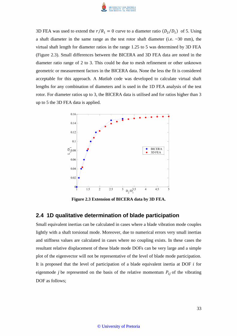
33

3D FEA was used to extend the ⁄ curve to a diameter ratio ⁄ of 5. Using

a shaft diameter in the same range as the test rotor shaft diameter (i.e. ~30 mm), the

virtual shaft length for diameter ratios in the range 1.25 to 5 was determined by 3D FEA

(Figure 2.3). Small differences between the BICERA and 3D FEA data are noted in the

diameter ratio range of 2 to 3. This could be due to mesh refinement or other unknown

geometric or measurement factors in the BICERA data. None the less the fit is considered

acceptable for this approach. A Matlab code was developed to calculate virtual shaft

lengths for any combination of diameters and is used in the 1D FEA analysis of the test

rotor. For diameter ratios up to 3, the BICERA data is utilised and for ratios higher than 3

up to 5 the 3D FEA data is applied.

Figure 2.3 Extension of BICERA data by 3D FEA.

2.4 1D qualitative determination of blade participation

Small equivalent inertias can be calculated in cases where a blade vibration mode couples

lightly with a shaft torsional mode. Moreover, due to numerical errors very small inertias

and stiffness values are calculated in cases where no coupling exists. In these cases the

resultant relative displacement of these blade mode DOFs can be very large and a simple

plot of the eigenvector will not be representative of the level of blade mode participation.

It is proposed that the level of participation of a blade equivalent inertia at DOF for

eigenmode be represented on the basis of the relative momentum of the vibrating

DOF as follows;

1 1.5 2 2.5 3 3.5 4 4.5 50

0.02

0.04

0.06

0.08

0.1

0.12

0.14

0.16

D2/D

1

Lv/D

1

BICERA3D FEA


34

| |

∑ | |

2.4-1

where is the total number of DOF. The blade participation factor is then

used to scale the blade mode DOF in the normalised eigenvector.

2.4-2

2.5 Full 3D FE modelling

3D finite element modelling is done using the commercial software package ANSYS

version 14.0. A high level of geometric detail is included in all cases to ensure good

accuracy. To this end all bolts, nuts and threaded holes are included. All geometry is

modelled to be parametric including blade stagger angle to allow for parametric studies as

well as updating of dimensions to as built values if required. The standard SI unit system

is used throughout.

Meshing is done using hexahedral and tetrahedral ANSYS element SOLID186. This 20

node element uses quadratic shape functions and has 20 nodes (Figure 2.4). Each node

has three translational degrees of freedom and has stress stiffening as well as large

deflection and large strain capabilities.

Homogenous and isotropic material properties for density, modulus of elasticity,

Poisson’s ratio, damping and thermal expansion coefficients can be defined (amongst

others). The default option of uniform reduced integration is used although no volumetric

locking is expected in the current work.

Bonded contact is applied between couplings and shafts. This form of contact implies no

sliding or separation of contact pairs and allows for linear solutions (required for modal

analysis).


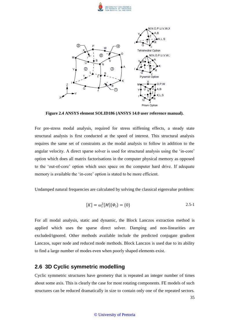
35

Figure 2.4 ANSYS element SOLID186 (ANSYS 14.0 user reference manual).

For pre-stress modal analysis, required for stress stiffening effects, a steady state

structural analysis is first conducted at the speed of interest. This structural analysis

requires the same set of constraints as the modal analysis to follow in addition to the

angular velocity. A direct sparse solver is used for structural analysis using the ‘in-core’

option which does all matrix factorisations in the computer physical memory as opposed

to the ‘out-of-core’ option which uses space on the computer hard drive. If adequate

memory is available the ‘in-core’ option is stated to be more efficient.

Undamped natural frequencies are calculated by solving the classical eigenvalue problem:

[ ] [ ]{ } { } 2.5-1

For all modal analysis, static and dynamic, the Block Lanczos extraction method is

applied which uses the sparse direct solver. Damping and non-linearities are

excluded/ignored. Other methods available include the predicted conjugate gradient

Lanczos, super node and reduced mode methods. Block Lanczos is used due to its ability

to find a large number of modes even when poorly shaped elements exist.

2.6 3D Cyclic symmetric modelling

Cyclic symmetric structures have geometry that is repeated an integer number of times

about some axis. This is clearly the case for most rotating components. FE models of such

structures can be reduced dramatically in size to contain only one of the repeated sectors.


36

Static structural as well as modal and pre-stressed modal analysis can be done using

cyclic symmetric models potentially resulting in significant time saving during the

solution process. Cyclic symmetry is applied in ANSYS by first modelling one complete

sector in a cylindrical coordinate system. A pair of matching surfaces on either side of the

sector is defined. Surfaces are referred to as high and low boundary edges. It is preferable,

although not required, that these surfaces have matching nodes i.e. the surfaces have

perfectly matching meshes. Matching meshes can be generated manually or by defining

cyclic symmetry before meshing is done. ANSYS then automatically attempts to match

the meshes. ANSYS applies the Duplicate Sector solving technique thus creating a

duplicate of the defined sector including all loads and constraints. Boundary nodes of

both the modelled and duplicate sectors are coupled using constraint equations of the

form;

{

} [

] {

}

Cyclic symmetric structures, e.g. disks, have vibration modes with areas of zero

displacement; these are referred to as nodal diameters. A mode with a nodal diameter of

0, also referred to as the umbrella mode, implies out of plane displacement of the outer

edge relative to the centre or in plane torsional displacement of the outer edge. The

harmonic index, or wave number, is an integer number that describes the variation of a

DOF spaced at angles equal to the sector angle. The nodal diameter may be the same as

the harmonic index but it is not always the case. A number of nodal diameter solutions

may exist for a given harmonic index. The relation between these two integer numbers

can be expressed as;

2.6-1

where;

= 0, 1, 2, …, ∞

= number of sectors such that

= harmonic index

In this study only the 0th nodal diameter is of interest and hence modal solutions for the

0th harmonic index only were calculated. Modal and pre-stressed modal analysis with 3D

CS models are conducted the same as for full 3D models.


37

2.7 Torsional properties of shafts and blades

The polar moment of inertia and torsional stiffness for a cylindrical solid shaft with

a diameter , length and shear modulus around its axis of rotation can be calculated

from (EPRI, 2005a);

2.7-1

2.7-2

Assuming a 1 DOF system the torsional natural frequency thereof can be calculated

from (Tse, Morse, and Hinkle, 1978);

√

2.7-3

Polar moment of inertia for a rectangular flat blade with a mass of , thickness and

width around an axis away from its centre of gravity can be calculated from (Roark

and Young, 1975);

2.7-4

2.8 Calculation of damping

Calculation of the damping factor in the time domain can be done using the log

decrement method. In this approach the displacement amplitude of two consecutive peaks

( and ) are measured in the time domain and the damping factor is calculated from

(Tse et al., 1978);

√ 2.8-1

with (

) 2.8-2


38

Damping can also be calculated in the frequency domain using the peak picking method

also referred to as the half power method. The frequency of the maximum amplitude ( )

of an isolated resonance peak in the FRF is taken as the natural frequency for the mode

( ). Frequencies at the half power point (| | √ are determined as (above ) and

(below ) from which the damping factor for the mode can be calculated from

(Meirovitch, 2001);

2.8-3

with

2.8-4

2.9 Campbell diagram

Campbell diagrams are used to plot the dependence of natural frequencies on speed.

Natural frequencies for blades and bladed disks have been shown to be affected by

rotational speed due to the stiffening effect of the centrifugal force on the blades. In this

work the effect on torsional frequencies, which can be affected by blade participation, is

investigated using Campbell diagrams. Natural frequencies are either measured or

calculated at various speeds in the range of interest and directly plotted on a graph.

Harmonic excitation lines, which are calculated as multiples of running speed, are also

shown on the same graph. Areas where the harmonic excitation lines cross a natural

frequency may be susceptible to resonance. Due to the occurrence of nodal diameters in

the case of bladed disks the interference diagram is also used. This is however not

considered here as only the 0 nodal diameters, which couple with torsional modes, are

considered.


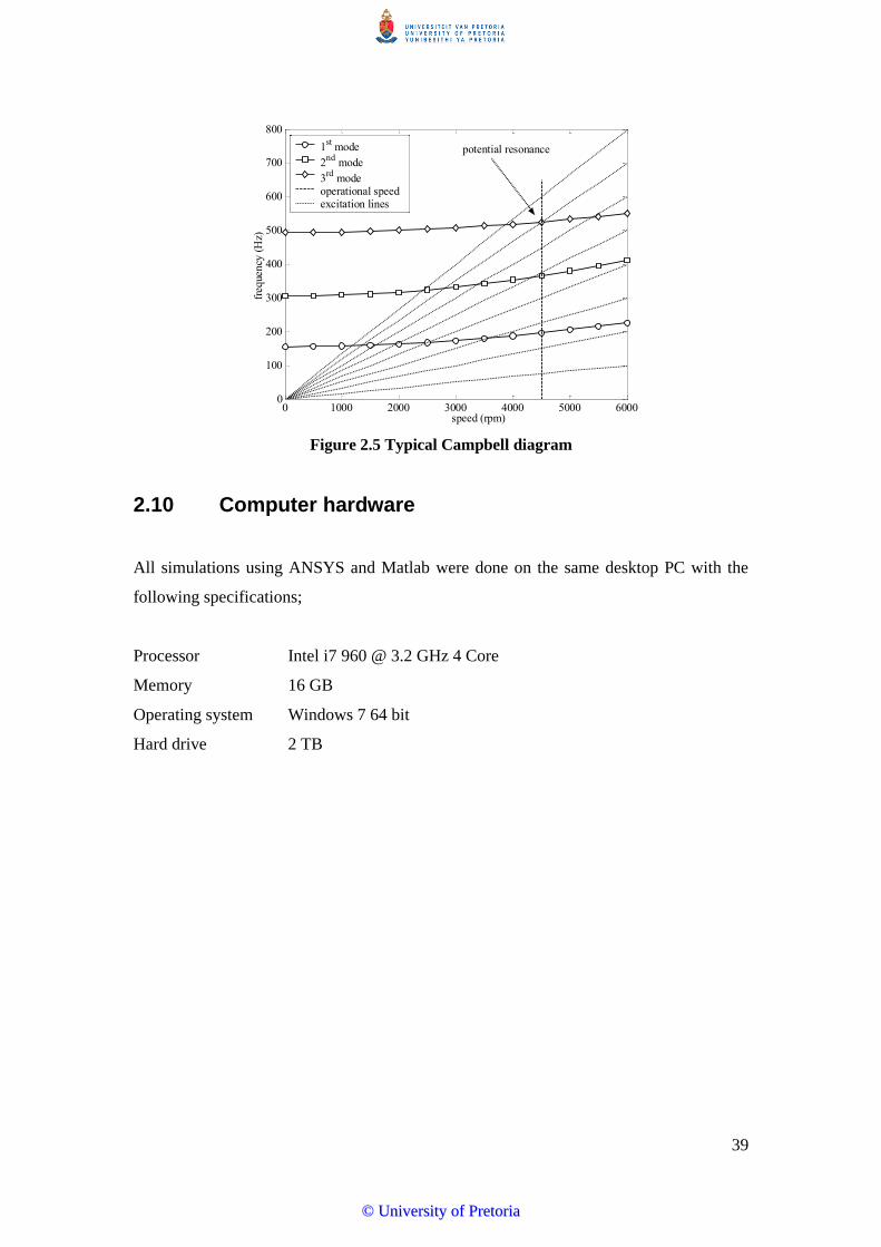
39

Figure 2.5 Typical Campbell diagram

2.10 Computer hardware

All simulations using ANSYS and Matlab were done on the same desktop PC with the

following specifications;

Processor Intel i7 960 @ 3.2 GHz 4 Core

Memory 16 GB

Operating system Windows 7 64 bit

Hard drive 2 TB

0 1000 2000 3000 4000 5000 60000

100

200

300

400

500

600

700

800

potential resonance

speed (rpm)

frequency

(H

z)

1st mode

2nd

mode

3rd

modeoperational speedexcitation lines


40

3. Experimental test rotor

3.1 Design and layout of test rotor

A test rotor was designed for laboratory testing and measurement of shaft torsional

vibration response under steady state operation as well as during forced excitation. Steady

state operation implies constant speed operation whilst forced excitation includes random

excitation, impulse loading and sudden speed step changes.

The rotor consists of a shaft, three disks, eight blade holders with blades and a drive end

(DE) coupling; all manufactured from EN8 carbon steel. In order to have flexibility in

configuration both disks were machined to accept the blade holders and blades. For all the

tests the blade holders and blades were fitted to disk #1 (disk on DE side). The blades can

be fitted in the 0, 45 or 90° position, known as the blade stagger angle, where 90° is the

position where the blade width is aligned with the tangential direction (or perpendicular

to the shaft centre line) as in Figure 3.1. The disk mounted on the NDE side (disk #3) is to

provide additional inertia at that end (see Figure 3.2).

Figure 3.1 Test rotor with blades at 90° (only shaft, disk #1 and #2 shown).

The shaft has a nominal diameter of 29 mm, but is stepped to a diameter of 30 mm and 31

mm for the bearing and disk landings respectively, with a total length of 880 mm. Both

disks #1 and #2 have a diameter of 150 mm and a width of 40 mm and are shrunk onto

the rotor whereas disk #3 is attached with a coupling (NDE coupling). Blades have a


41

width of 26 mm, a thickness of 2.1 mm and a length of 110 mm (measured from the top

of the blade holder).

Rotational drive and torsional excitation are accomplished through a drive system

consisting of a DC motor and a digital controller. The rotor is coupled to the DC motor by

a flanged coupling and is supported by two self-aligning roller element bearings. The

complete setup is mounted on a vibrationally isolated test bed mounted on springs. For

additional details on the rotor geometry please refer to Appendix A.

Figure 3.2 Photograph of test rotor in the test bench.

3.2 Drive and torsional excitation system

A 3 kW Brook Crompton DC motor with a maximum armature voltage and rotational

speed of 180V and 3000 rpm is used to drive the test rotor. The motor is controlled with a

DCREG4 digital controller manufactured by Elettronica Santerno and designed for

controlling field and armature current of DC motors for speed or torque control. Control

loops for speed (or armature voltage) and current are used as well as a regulator for the

motor stator field. The DCREG4 allows for fully reversible operation i.e. the motor can

act to drive or brake the test rotor.

Based on initial performance tests it was decided to use speed control instead of torque

control as this provided faster response as well as more stable speed control. The field

current can be regulated in fixed or field weakening mode which can be used to reduce


42

energy consumption when no drive is required for a set period of time. Fixed field current

regulation was selected (field current fixed at 0.49 A).

Speed feedback for the speed control loop can be obtained from an encoder, tachometer

or the armature voltage. Although a Hengstler R-158/D1000ED rotary encoder was fitted

to the NDE side of the motor armature and used for speed indication available through an

analogue output (nOut), it led to unpredictable speed response and was not used for speed

control. Analogue speed output signal nOut is discussed in more detail in section 3.3.8. It

was decided to use armature voltage for speed feedback. In this control mode the speed is

controlled indirectly through the armature voltage where a maximum voltage of 180 V

relates to approximately to 3000 rpm. A simplified diagram of the control system speed

control loop is shown in Figure 3.3.

A voltage signal/s from a number of sources is conditioned, summed and filtered to

produce a speed reference voltage, or in this case an armature voltage reference that

ranges from -10 to +10 V for an armature voltage of ±180 V (which relates to ±3000

rpm). Where required the mean speed ( ) was set using the DCREG4 potentiometer.

One of the two analogue inputs was used to supply a dynamic speed reference signal

( ), from an external source, that is summed to as well as any offset ( if

required to give a speed reference signal ( ). The difference between and the

feedback speed ( ) is the speed error ( ). After applying a low pass filter (inactive

in this work) to a speed setpoint ( ) based on the speed loop proportional gain

( and integral time ( ) is calculated. Based on , the current feedback signal,

current loop proportional gain and integral time constants, a current setpoint is calculated

which is used by the motor controller to drive the motor.

A ±10 V signal proportional to the armature current referred to as IOut is also available

from the DCREG4. A signal of 6.67 V corresponds to the rated capacity of the drive (20

A) which implies a sensitivity of 3 A/V. Local displays of nOut and IOut have a 12 bit

resolution. Although the rated field current of the DCREG4 is 5 A the field current

supplied to the motor stator was set at 0.49 A. The motor rated field current is 0.6 A. The

torque developed by the motor can be calculated as the product of the armature current

and the field current. Based on this the nominal maximum torque at full motor armature

rated current is 10 N.m. Optimum values for the relevant settings of the speed control

loop as described above to obtain a fast speed response, minimal speed over/under shoot


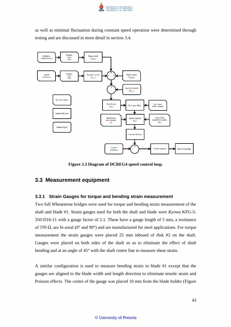
43

as well as minimal fluctuation during constant speed operation were determined through

testing and are discussed in more detail in section 3.4.

Figure 3.3 Diagram of DCREG4 speed control loop.

3.3 Measurement equipment

3.3.1 Strain Gauges for torque and bending strain measurement

Two full Wheatstone bridges were used for torque and bending strain measurement of the

shaft and blade #1. Strain gauges used for both the shaft and blade were Kyowa KFG-5-

350-D16-11 with a gauge factor of 2.1. These have a gauge length of 5 mm, a resistance

of 350 Ω, are bi-axial (0° and 90°) and are manufactured for steel applications. For torque

measurement the strain gauges were placed 25 mm inboard of disk #2 on the shaft.

Gauges were placed on both sides of the shaft so as to eliminate the effect of shaft

bending and at an angle of 45° with the shaft centre line to measure shear strain.

A similar configuration is used to measure bending strain in blade #1 except that the

gauges are aligned to the blade width and length direction to eliminate tensile strain and

Poisson effects. The centre of the gauge was placed 10 mm from the blade holder (Figure


44

3.4). Strain gauges and wiring were glued down using Kyowa CC33A cyano-acrylate glue

and wired to an Accumetrics telemetry system.

Figure 3.4 Position of strain gauges on the shaft (left) and blade (right).

3.3.2 Accumetrics Telemetry System

The Accumetrics AT-500 telemetry system has a frequency bandwidth of up to 1 kHz.

This system has a single channel output with the transmitter and battery weighing 35.5 g

and 19.6 g respectively. A connection block used to connect the strain gauges weighed an

additional 11.7 g. The telemetry system, battery and connection block was held in place

with multiple layers of reinforced strapping tape. A magnetic base clamp was used to

locate the receiver aerial as close as possible to the transmitter.


45

Figure 3.5 Shaft strain gauge positions and Accumetrics telemetry system.

Calibration of the telemetry system was done using a HBM Kalibriergerat K3607 strain

gauge bridge calibrator (serial #42077) and a HP 3465A digital multimeter (serial #553).

Using a sensitivity of 0.5 mV/V the system calibration was found to be acceptable (Figure

3.6). The response is linear between -80 and +90% of the input signal.

Figure 3.6 Calibration of Accumetrics telemetry system.

For torque measurements using a full bridge configuration it can be shown that the

indicated strain ( ) and measured torque ( ) can be calculated from (Hoffmann, 1989);


46

3.3-1

3.3-2

where;

= telemetry system output voltage

= gauge factor

= bridge excitation voltage

= system gain

= modulus of elasticity

= shaft radius

= Poisson ratio

Using the Accumetrics telemetry system the shaft and blade strain gauge bridges were

balanced using a short length of Constantan wire. The accuracy of these installations was

tested by applying a known torque or bending moment to the shaft and blade respectively.

A torque arm with a length of 0.3 m was mounted on the non-drive end side coupling of

the shaft. The shaft was fixed in the circumferential direction at the drive end side

coupling. Calibrated weights were added incrementally and the resultant torque calculated

from the measured strain correlated well with actual applied torque (Figure 3.7). A

theoretical sensitivity factor of 11.08 N.m/V was calculated using equation 3.3-2.

Calibration resulted in a small change to 12.47 N.m/V.

Figure 3.7 Calibration of shaft strain gauge bridge and telemetry system.


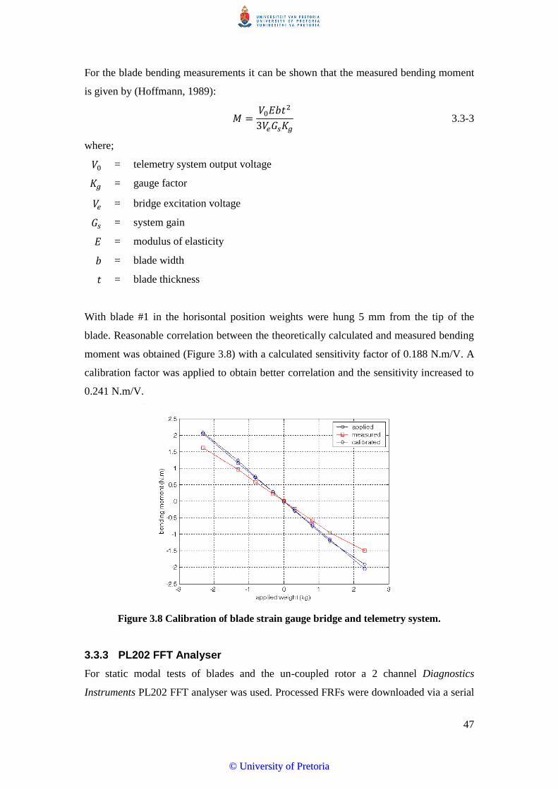
47

For the blade bending measurements it can be shown that the measured bending moment

is given by (Hoffmann, 1989):

3.3-3

where;

= telemetry system output voltage

= gauge factor

= bridge excitation voltage

= system gain

= modulus of elasticity

= blade width

= blade thickness

With blade #1 in the horisontal position weights were hung 5 mm from the tip of the

blade. Reasonable correlation between the theoretically calculated and measured bending

moment was obtained (Figure 3.8) with a calculated sensitivity factor of 0.188 N.m/V. A

calibration factor was applied to obtain better correlation and the sensitivity increased to

0.241 N.m/V.

Figure 3.8 Calibration of blade strain gauge bridge and telemetry system.

3.3.3 PL202 FFT Analyser

For static modal tests of blades and the un-coupled rotor a 2 channel Diagnostics

Instruments PL202 FFT analyser was used. Processed FRFs were downloaded via a serial


48

link to a PC and further processed using Matlab for presentation. Connections and

settings for specific tests are discussed in the relevant sections.

3.3.4 PCB Piezotronics Impact Hammer

All modal tests were conducted with a model 086C03 PCB Piezotronics impact hammer

serial number 8133 with a sensitivity of 2.15 mV/N. Where the PL202 analyser was used

a PCB Piezotronics model 480C02 ICP sensor power unit was used. When the Oros

OR35 analyser (discussed below) was used the hammer was coupled directly to the OR35

which can drive ICP transducers directly.

3.3.5 Polytec Portable Digital Vibrometer PDV-100

A Polytec PDV-100 single point laser vibrometer (LV) was used to measure blade

response for modal tests when exciting the blade directly or indirectly via the shaft using

the impact hammer. The PDV-100 has a frequency range of 0.05 Hz to 22 kHz and was

set to a range of 500 mm/s which implies a scaling factor of 125 mm/s/V for the output

voltage of ±4 V. The low pass filter was set at 1 kHz and the 100 Hz high pass filter was

activated.

3.3.6 Polytec Torsional Laser Vibrometer OFV-4000

For non-contact measurement of torsional vibration a Polytec OFV-400 sensor head with

an OFV-4000 controller was used. Torsional velocity is measured based on laser

interferometry and torsional displacement is then internally calculated by integration. The

system has a frequency range of 0.5 Hz to 10 kHz. Rotational speeds of up to 11000 rpm

are measureable and angular resolution is claimed to be very high (no limit specified).The

laser head was mounted on a tripod ~400 mm from the shaft surface with the two laser

beams focussed at approximately equal distances from either side of the shaft centreline

(i.e. symmetrically) to ensure good balance and that the complete speed range can be

measured. DC rotation rate was set to fast in order to capture the rotational speed during

transient conditions (e.g. during impulse excitation), which implies a time constant of 100

µs. Rotational speed is available via a 1 mV/rpm analogue voltage output from the

controller. A scale factor of 10 °/s/V, 100 °/s/V, 1000 °/s/V or 6000 °/s/V can be selected

for angular vibration velocity measurements. Low and high pass filters are available and

were used where indicated.


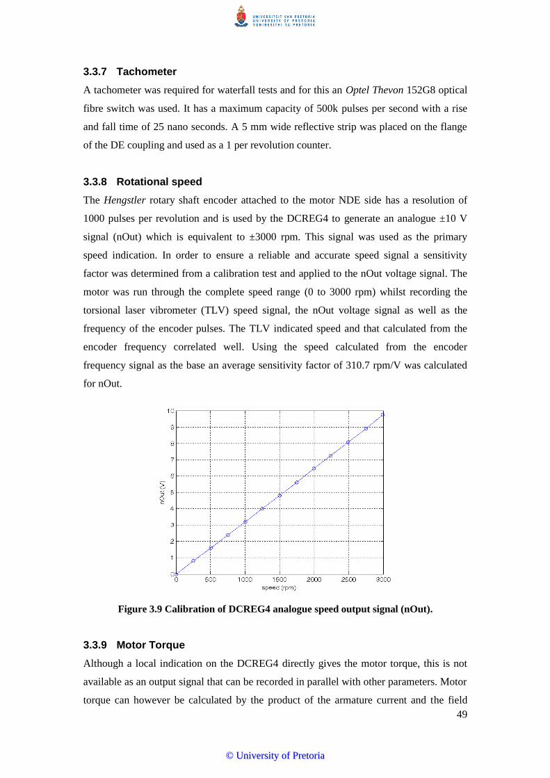
49

3.3.7 Tachometer

A tachometer was required for waterfall tests and for this an Optel Thevon 152G8 optical

fibre switch was used. It has a maximum capacity of 500k pulses per second with a rise

and fall time of 25 nano seconds. A 5 mm wide reflective strip was placed on the flange

of the DE coupling and used as a 1 per revolution counter.

3.3.8 Rotational speed

The Hengstler rotary shaft encoder attached to the motor NDE side has a resolution of

1000 pulses per revolution and is used by the DCREG4 to generate an analogue ±10 V

signal (nOut) which is equivalent to ±3000 rpm. This signal was used as the primary

speed indication. In order to ensure a reliable and accurate speed signal a sensitivity

factor was determined from a calibration test and applied to the nOut voltage signal. The

motor was run through the complete speed range (0 to 3000 rpm) whilst recording the

torsional laser vibrometer (TLV) speed signal, the nOut voltage signal as well as the

frequency of the encoder pulses. The TLV indicated speed and that calculated from the

encoder frequency correlated well. Using the speed calculated from the encoder

frequency signal as the base an average sensitivity factor of 310.7 rpm/V was calculated

for nOut.

Figure 3.9 Calibration of DCREG4 analogue speed output signal (nOut).

3.3.9 Motor Torque

Although a local indication on the DCREG4 directly gives the motor torque, this is not

available as an output signal that can be recorded in parallel with other parameters. Motor

torque can however be calculated by the product of the armature current and the field


50

current. Armature current is also only available locally (no output signal) but the IOut

signal is proportional to the armature current and available as a voltage signal. As

discussed in section 3.2 the specified sensitivity of this signal is 3 A/V. A calibration test

was done to confirm and refine this value (Figure 3.10).

Figure 3.10 Calibration of armature current (from IOut).

With the rotor coupled the indicated armature current (Iarm), motor speed, indicated

torque, indicated field current and motor current (IOut) was recorded at speeds from 0 to

2000 rpm. A plot of the indicated armature current vs. IOut shows a linear relationship

(Figure 3.11). A first order polynomial was fitted to the data and the sensitivity found to

be 3.22 A/V. Torque calculated from the indicated armature current as well as based on

IOut correlated well with the indicated torque. Note that the indicated field current

remained constant at 0.49 A.

0 0.1 0.2 0.3 0.4 0.5 0.6 0.7 0.8 0.90

0.5

1

1.5

2

2.5

3

IOut (V)

arm

atu

re c

urr

en

t (A

)

measured

polynomial fit


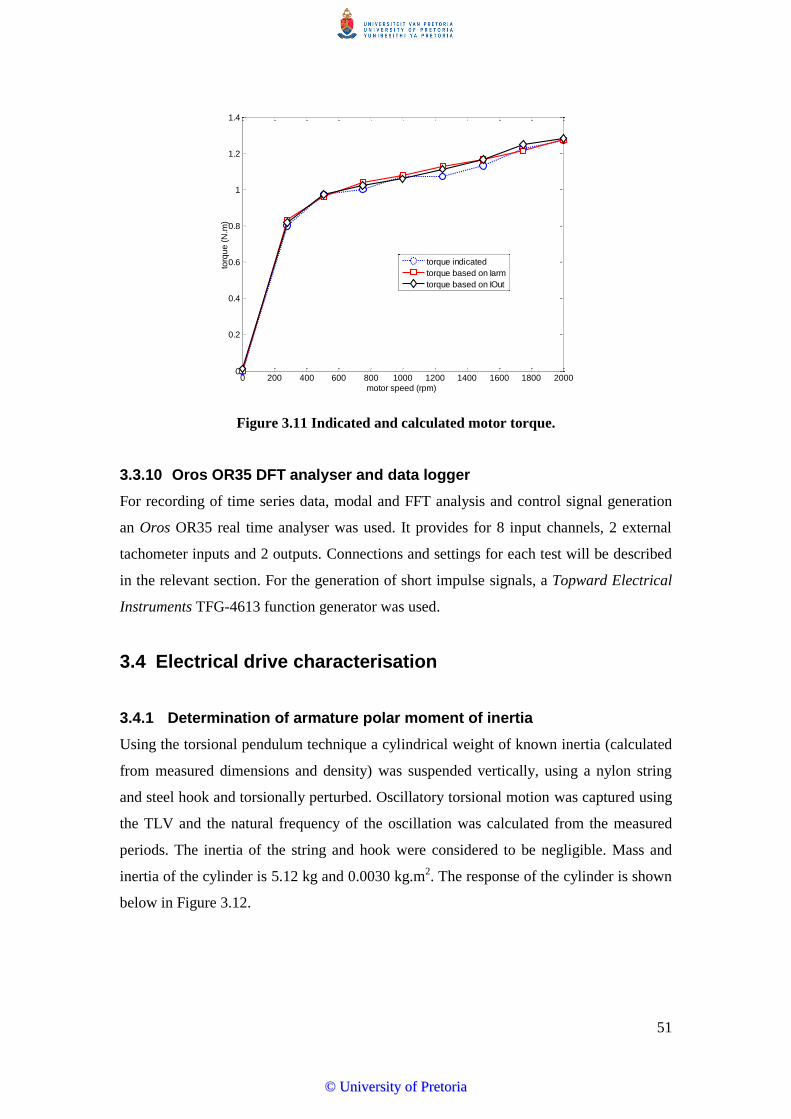
51

Figure 3.11 Indicated and calculated motor torque.

3.3.10 Oros OR35 DFT analyser and data logger

For recording of time series data, modal and FFT analysis and control signal generation

an Oros OR35 real time analyser was used. It provides for 8 input channels, 2 external

tachometer inputs and 2 outputs. Connections and settings for each test will be described

in the relevant section. For the generation of short impulse signals, a Topward Electrical

Instruments TFG-4613 function generator was used.

3.4 Electrical drive characterisation

3.4.1 Determination of armature polar moment of inertia

Using the torsional pendulum technique a cylindrical weight of known inertia (calculated

from measured dimensions and density) was suspended vertically, using a nylon string

and steel hook and torsionally perturbed. Oscillatory torsional motion was captured using

the TLV and the natural frequency of the oscillation was calculated from the measured

periods. The inertia of the string and hook were considered to be negligible. Mass and

inertia of the cylinder is 5.12 kg and 0.0030 kg.m2. The response of the cylinder is shown

below in Figure 3.12.

0 200 400 600 800 1000 1200 1400 1600 1800 20000

0.2

0.4

0.6

0.8

1

1.2

1.4

motor speed (rpm)

torq

ue

(N

.m)

torque indicated

torque based on Iarm

torque based on IOut


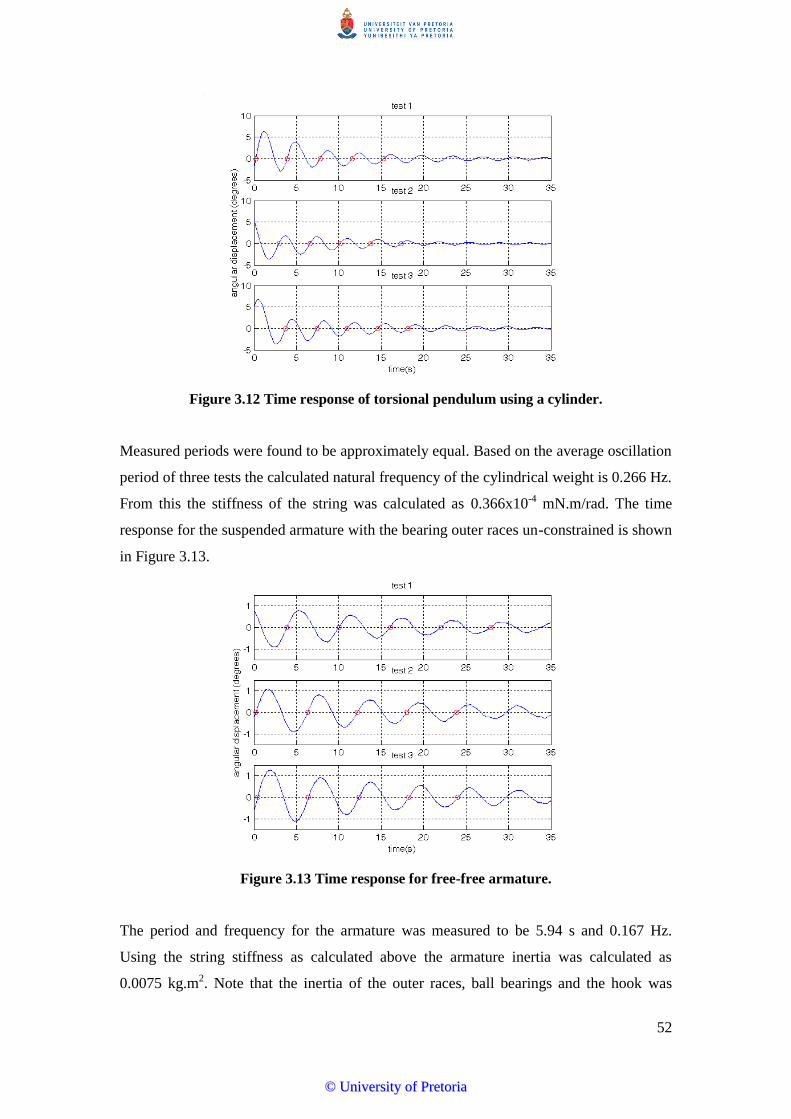
52

Figure 3.12 Time response of torsional pendulum using a cylinder.

Measured periods were found to be approximately equal. Based on the average oscillation

period of three tests the calculated natural frequency of the cylindrical weight is 0.266 Hz.

From this the stiffness of the string was calculated as 0.366x10-4 mN.m/rad. The time

response for the suspended armature with the bearing outer races un-constrained is shown

in Figure 3.13.

Figure 3.13 Time response for free-free armature.

The period and frequency for the armature was measured to be 5.94 s and 0.167 Hz.

Using the string stiffness as calculated above the armature inertia was calculated as

0.0075 kg.m2. Note that the inertia of the outer races, ball bearings and the hook was


53

included in this approach. The above test was repeated with the outer bearing races

constrained as depicted in Figure 3.14.

Figure 3.14 Suspended armature with bearing outer races constrained.

The time response is shown below in Figure 3.15. As can be seen the periods of

oscillation are not constant and only two to three oscillations are recorded. This is likely

due to bearing friction. An alternative approach was used where the flexible string was

replaced with a stiffer mild steel rod 2 mm in diameter. The experimental setup allows for

the length of the rod and thus the torsional stiffness to be varied. Figure 3.16 shows the

experimental setup with the armature in the horisontal position and the bearing outer

races constrained. Torsional stiffness of the rod can be calculated directly from the

diameter, length and bulk modulus thereof. Time series responses for three rod lengths

(i.e. 150, 340 and 430 mm) were measured and recorded using the TLV and OR35. Three

tests per rod length were conducted and the average period determined. It was found that

the periods for the first two oscillations tended to be longer than the subsequent

oscillations and these were ignored in the calculations. Time response for a rod length of

150 mm is shown below in Figure 3.17.


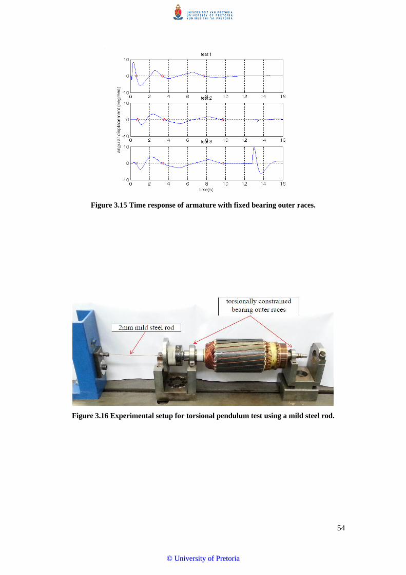
54

Figure 3.15 Time response of armature with fixed bearing outer races.

Figure 3.16 Experimental setup for torsional pendulum test using a mild steel rod.


55

Figure 3.17 Armature time response for 150 mm rod.

Based on the natural frequencies calculated from the oscillation periods and the calculated

rod stiffness, the armature inertia for the three cases was calculated as 0.0078, 0.0078 and

0.0079 kg.m2. This correlates well with the value of 0.0075 kg.m2 determined using the

torsional pendulum approach with a flexible string. An inertia value of 0.0078 kg.m2 was

used in all further calculations.

3.4.2 Control loop response and drive vibrational characteristics

A large number of programmable control loop settings are available through the

DCREG4 control system. This was reduced by initial testing to the variables as discussed

in section 3.2. Further testing was conducted to optimise these selected parameters in

order to obtain a fast speed response for transient conditions (e.g. speed step change) but

also to obtain stable response during constant speed operation. With the low pass filter on

disabled, the remaining two parameters to optimise were the speed loop proportional

gain ( ) and integral time ( ). Using the DCREG4 potentiometer the mean speed was

set to approximately 1000 rpm with always zero. A voltage signal equivalent to a

speed step of ~300 rpm was generated by the OR35 and connected to the DCREG4

analogue input. For each step the speed error ( motor current (IOut), motor speed

(nOut) and speed step signal were recorded at a sampling rate of 51.2k samples per

second. Low values of proportional gain and integral time resulted in a slow speed

response that is also lightly damped with significant over/under shoot (Figure 3.18). Low

proportional gain with a high time integral value results in a slow response that is highly


56

damped with no overshoot (Figure 3.19). A high proportional gain and a low integral time

of 8 and 0.4 s resulted in a fast response with minimal overshoot and stable response at

constant speed. Using these settings, the response of the drive system to 300 rpm speed

steps from a mean speed of 250 to 2500 rpm in steps of 250 rpm was measured. In each

case the FRF of the speed signal (nOut) with reference to the control signal (SigGen) was

calculated to determine the frequency response of the drive system.

Figure 3.18 Response of drive for =0.1 and =0.09 s.

Figure 3.19 Response of drive for =0.5 and =5 s.


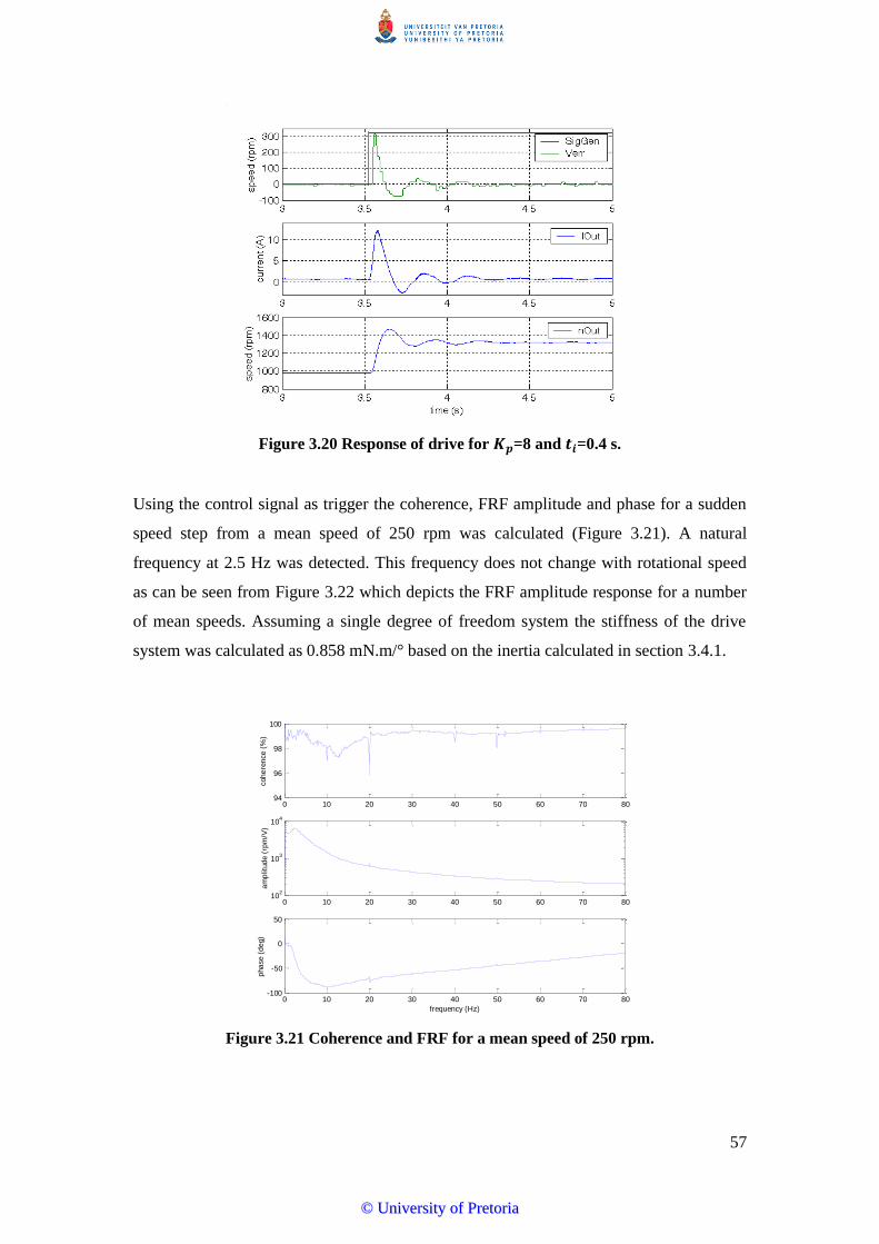
57

Figure 3.20 Response of drive for =8 and =0.4 s.

Using the control signal as trigger the coherence, FRF amplitude and phase for a sudden

speed step from a mean speed of 250 rpm was calculated (Figure 3.21). A natural

frequency at 2.5 Hz was detected. This frequency does not change with rotational speed

as can be seen from Figure 3.22 which depicts the FRF amplitude response for a number

of mean speeds. Assuming a single degree of freedom system the stiffness of the drive

system was calculated as 0.858 mN.m/° based on the inertia calculated in section 3.4.1.

Figure 3.21 Coherence and FRF for a mean speed of 250 rpm.

0 10 20 30 40 50 60 70 8094

96

98

100

coh

ere

nce (

%)

0 10 20 30 40 50 60 70 8010

2

103

104

am

plitu

de

(rp

m/V

)

0 10 20 30 40 50 60 70 80-100

-50

0

50

pha

se

(d

eg)

frequency (Hz)


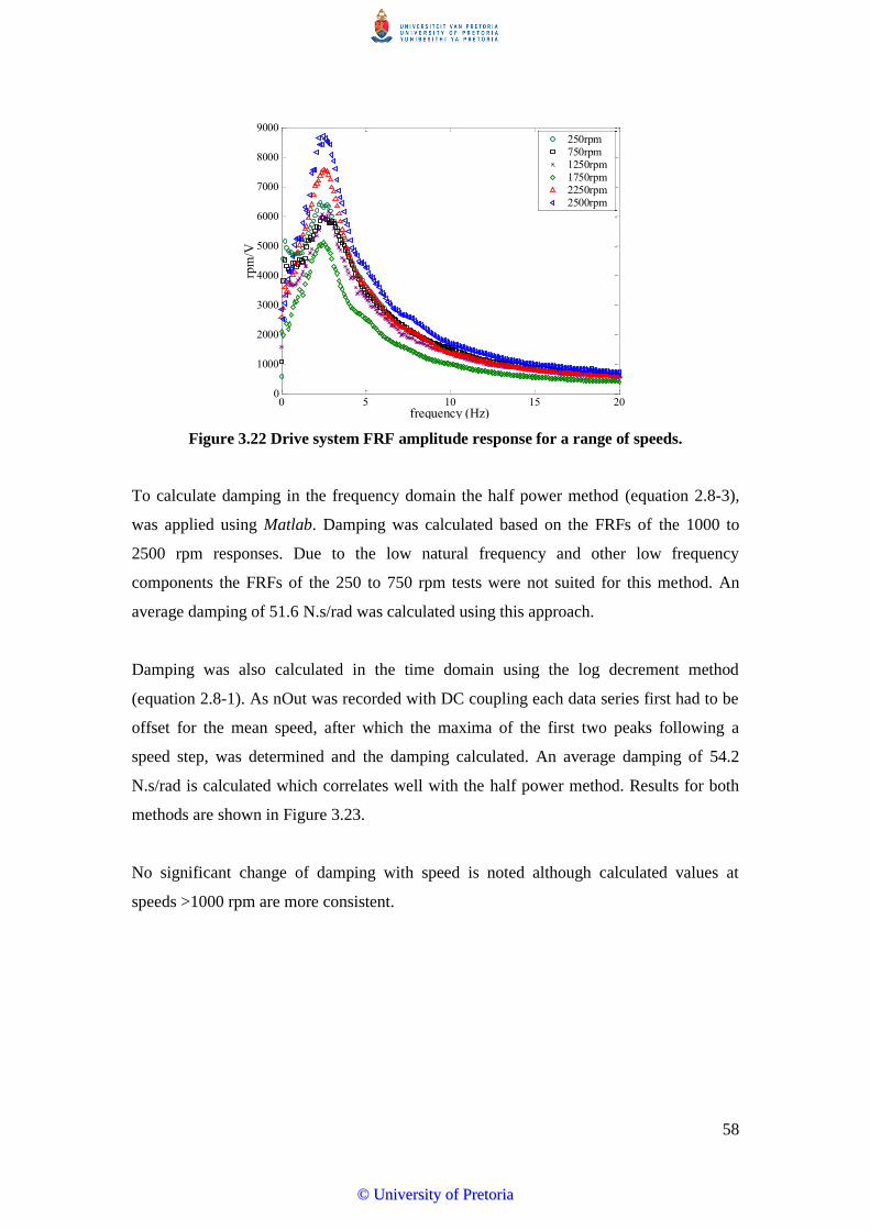
58

Figure 3.22 Drive system FRF amplitude response for a range of speeds.

To calculate damping in the frequency domain the half power method (equation 2.8-3),

was applied using Matlab. Damping was calculated based on the FRFs of the 1000 to

2500 rpm responses. Due to the low natural frequency and other low frequency

components the FRFs of the 250 to 750 rpm tests were not suited for this method. An

average damping of 51.6 N.s/rad was calculated using this approach.

Damping was also calculated in the time domain using the log decrement method

(equation 2.8-1). As nOut was recorded with DC coupling each data series first had to be

offset for the mean speed, after which the maxima of the first two peaks following a

speed step, was determined and the damping calculated. An average damping of 54.2

N.s/rad is calculated which correlates well with the half power method. Results for both

methods are shown in Figure 3.23.

No significant change of damping with speed is noted although calculated values at

speeds >1000 rpm are more consistent.

0 5 10 15 200

1000

2000

3000

4000

5000

6000

7000

8000

9000

frequency (Hz)

rpm

/V

250rpm750rpm1250rpm1750rpm2250rpm2500rpm


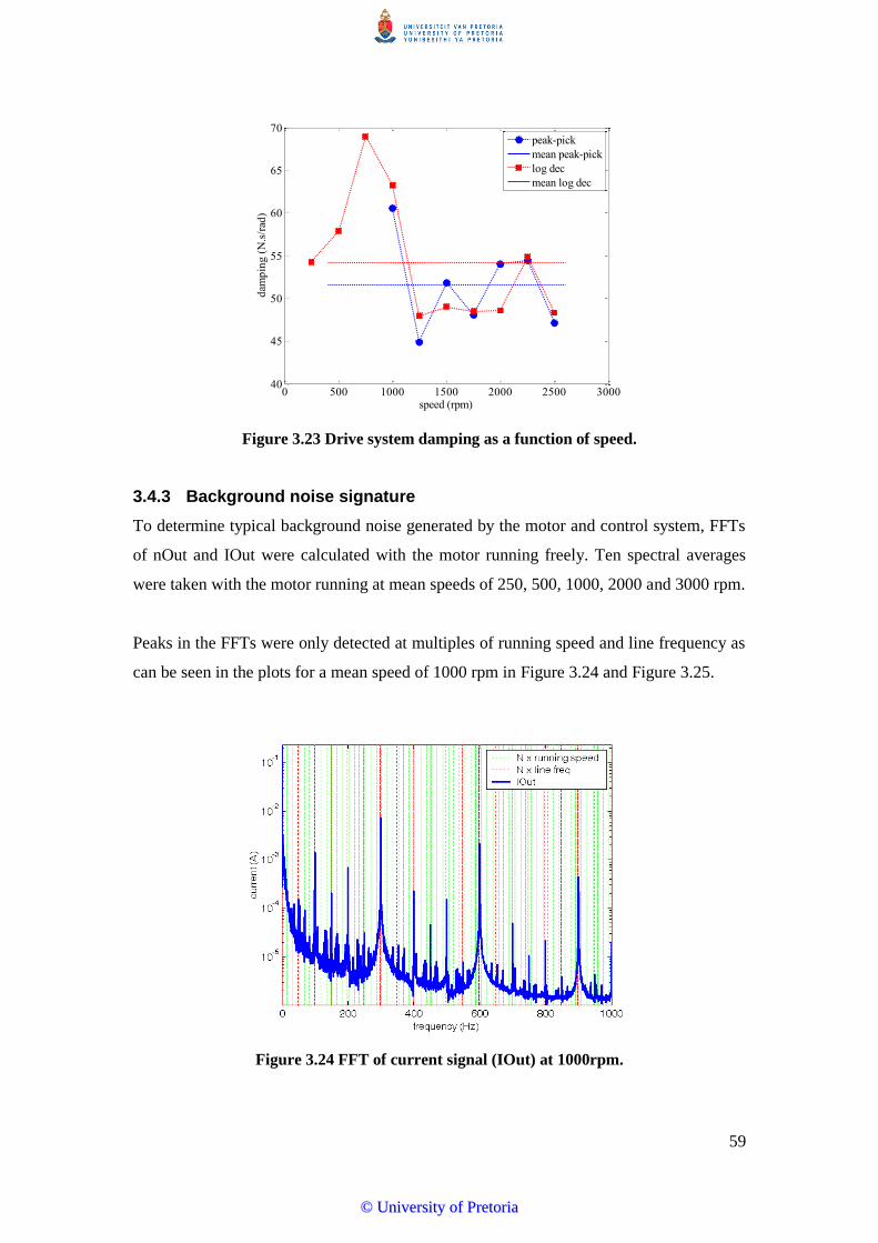
59

Figure 3.23 Drive system damping as a function of speed.

3.4.3 Background noise signature

To determine typical background noise generated by the motor and control system, FFTs

of nOut and IOut were calculated with the motor running freely. Ten spectral averages

were taken with the motor running at mean speeds of 250, 500, 1000, 2000 and 3000 rpm.

Peaks in the FFTs were only detected at multiples of running speed and line frequency as

can be seen in the plots for a mean speed of 1000 rpm in Figure 3.24 and Figure 3.25.

Figure 3.24 FFT of current signal (IOut) at 1000rpm.

0 500 1000 1500 2000 2500 300040

45

50

55

60

65

70

speed (rpm)

dam

pin

g (

N.s

/rad

)

peak-pick

mean peak-pick

log dec

mean log dec


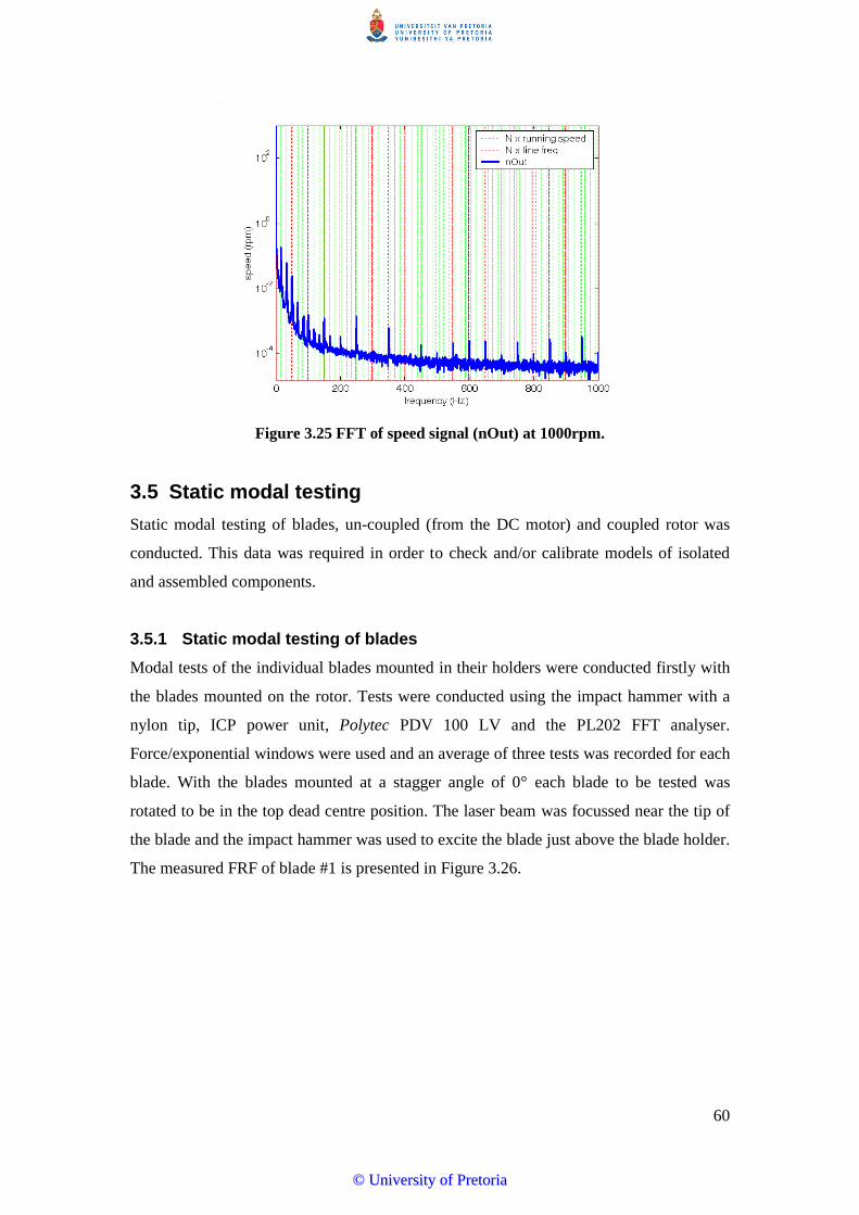
60

Figure 3.25 FFT of speed signal (nOut) at 1000rpm.

3.5 Static modal testing

Static modal testing of blades, un-coupled (from the DC motor) and coupled rotor was

conducted. This data was required in order to check and/or calibrate models of isolated

and assembled components.

3.5.1 Static modal testing of blades

Modal tests of the individual blades mounted in their holders were conducted firstly with

the blades mounted on the rotor. Tests were conducted using the impact hammer with a

nylon tip, ICP power unit, Polytec PDV 100 LV and the PL202 FFT analyser.

Force/exponential windows were used and an average of three tests was recorded for each

blade. With the blades mounted at a stagger angle of 0° each blade to be tested was

rotated to be in the top dead centre position. The laser beam was focussed near the tip of

the blade and the impact hammer was used to excite the blade just above the blade holder.

The measured FRF of blade #1 is presented in Figure 3.26.


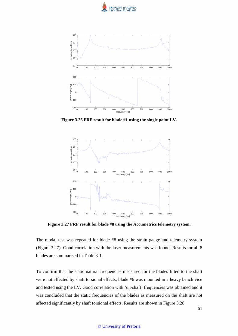
61

Figure 3.26 FRF result for blade #1 using the single point LV.

Figure 3.27 FRF result for blade #8 using the Accumetrics telemetry system.

The modal test was repeated for blade #8 using the strain gauge and telemetry system

(Figure 3.27). Good correlation with the laser measurements was found. Results for all 8

blades are summarised in Table 3-1.

To confirm that the static natural frequencies measured for the blades fitted to the shaft

were not affected by shaft torsional effects, blade #6 was mounted in a heavy bench vice

and tested using the LV. Good correlation with ‘on-shaft’ frequencies was obtained and it

was concluded that the static frequencies of the blades as measured on the shaft are not

affected significantly by shaft torsional effects. Results are shown in Figure 3.28.

0 100 200 300 400 500 600 700 800 900 100010

-4

10-3

10-2

10-1

100

norm

alise

d a

mp

litu

de

0 100 200 300 400 500 600 700 800 900 1000-200

-100

0

100

200

frequency [Hz]

pha

se

an

gle

[de

g]

0 100 200 300 400 500 600 700 800 900 100010

-4

10-3

10-2

10-1

100

frequency [Hz]

norm

alise

am

plitu

de

0 100 200 300 400 500 600 700 800 900 1000-200

-100

0

100

200

frequency [Hz]

pha

se

an

gle

[de

g]


62

Figure 3.28 Blade #6 response on shaft and in bench vice using the LV.

Table 3-1 Frequency results for static blade modal tests.

Mode # Blade

#1

Blade

#2

Blade

#3

Blade

#4

Blade

#5

Blade

#6

Blade

#7

Blade

#8

B1 (Hz) 142.5 145 145 145 145 145 145 142.5

B2 (Hz) 902.5 915 902.5 905 907.5 910 912.5 892.5

The average natural frequencies for the 1st and 2nd blade modes were found to be 144.6

and 907.9 Hz. Note that the frequencies for blade #8 are slightly lower. This is most

likely due to the additional mass of the strain gauge wiring.

Damping of the 1st and 2nd blade modes was calculated using the half power method and

the average for all blades was found to be 3.6 and 0.68 % respectively.

3.5.2 Armature torsional vibration modes

Modal testing of the motor armature was conducted using the impact hammer, TLV and

OR35. Tangential impacts imparted on a bolt tightly fastened in one of the DE coupling

key grub screw holes at a diameter of 59 mm were used for torsional excitation in all

cases. Torsional vibration measurements were taken at six positions as indicated in Figure

3.29. The armature was placed on two supports with the bearing outer races constrained

in the torsional direction. Force and response windows were applied to the hammer and

TLV angular velocity responses respectively. The TLV sensitivity was set to 100 mV/°/s.

0 100 200 300 400 500 600 700 800 900 100010

-4

10-3

10-2

10-1

100

norm

alise

d a

mp

litu

de

on shaft

in bench vice

0 100 200 300 400 500 600 700 800 900 1000-200

-100

0

100

200

frequency [Hz]

pha

se

an

gle

[de

g]


63

Figure 3.29 TLV measurement positions on armature.

To ensure all possible modes were captured both the low pass and high pass filter of the

TLV were disabled and the OR35 was set to a frequency range of 10 kHz. With 6401

lines used a frequency resolution of 1.5625 Hz was obtained. Spectral averaging was used

and the average of three tests per position was recorded. The time series response

measured at the DE coupling and its FRF is depicted in Figure 3.30 and Figure 3.31.

Figure 3.30 Response at armature DE coupling.


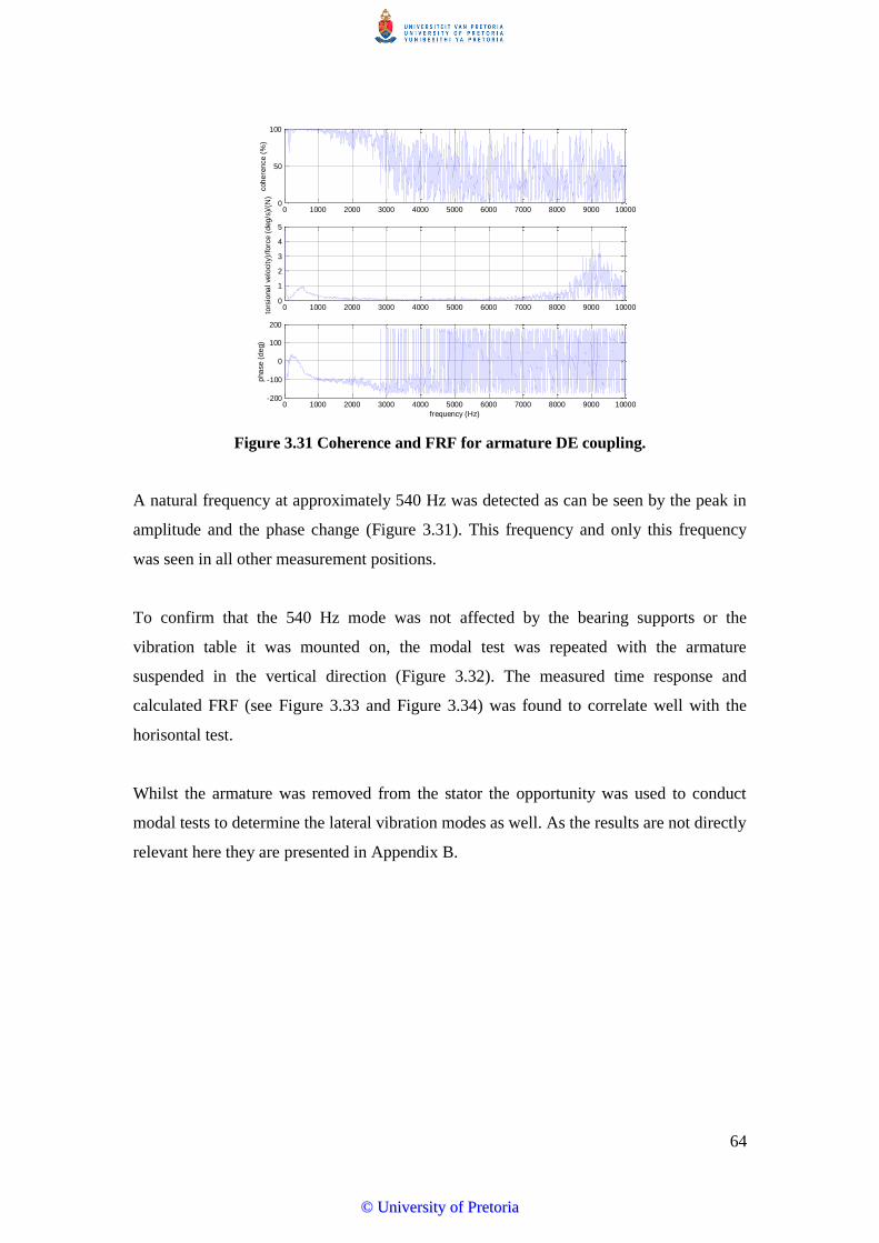
64

Figure 3.31 Coherence and FRF for armature DE coupling.

A natural frequency at approximately 540 Hz was detected as can be seen by the peak in

amplitude and the phase change (Figure 3.31). This frequency and only this frequency

was seen in all other measurement positions.

To confirm that the 540 Hz mode was not affected by the bearing supports or the

vibration table it was mounted on, the modal test was repeated with the armature

suspended in the vertical direction (Figure 3.32). The measured time response and

calculated FRF (see Figure 3.33 and Figure 3.34) was found to correlate well with the

horisontal test.

Whilst the armature was removed from the stator the opportunity was used to conduct

modal tests to determine the lateral vibration modes as well. As the results are not directly

relevant here they are presented in Appendix B.

0 1000 2000 3000 4000 5000 6000 7000 8000 9000 100000

1

2

3

4

5

tors

iona

l ve

loci

ty)/

forc

e (

deg

/s)/

(N)

0 1000 2000 3000 4000 5000 6000 7000 8000 9000 10000-200

-100

0

100

200

frequency (Hz)

pha

se

(d

eg)

0 1000 2000 3000 4000 5000 6000 7000 8000 9000 100000

50

100

coh

ere

nce (

%)


65

Figure 3.32 Armature modal test in vertical position.

Figure 3.33 Time response measured for the suspended armature.


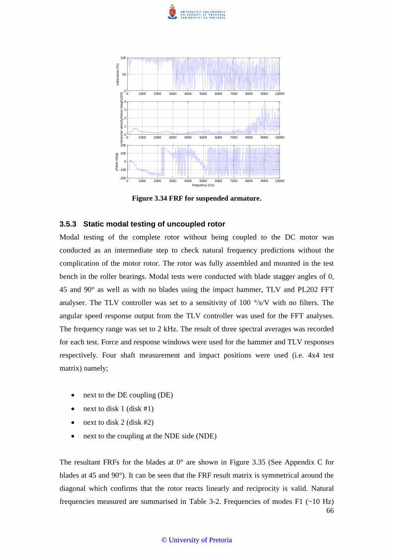
66

Figure 3.34 FRF for suspended armature.

3.5.3 Static modal testing of uncoupled rotor

Modal testing of the complete rotor without being coupled to the DC motor was

conducted as an intermediate step to check natural frequency predictions without the

complication of the motor rotor. The rotor was fully assembled and mounted in the test

bench in the roller bearings. Modal tests were conducted with blade stagger angles of 0,

45 and 90° as well as with no blades using the impact hammer, TLV and PL202 FFT

analyser. The TLV controller was set to a sensitivity of 100 °/s/V with no filters. The

angular speed response output from the TLV controller was used for the FFT analyses.

The frequency range was set to 2 kHz. The result of three spectral averages was recorded

for each test. Force and response windows were used for the hammer and TLV responses

respectively. Four shaft measurement and impact positions were used (i.e. 4x4 test

matrix) namely;

next to the DE coupling (DE)

next to disk 1 (disk #1)

next to disk 2 (disk #2)

next to the coupling at the NDE side (NDE)

The resultant FRFs for the blades at 0° are shown in Figure 3.35 (See Appendix C for

blades at 45 and 90°). It can be seen that the FRF result matrix is symmetrical around the

diagonal which confirms that the rotor reacts linearly and reciprocity is valid. Natural

frequencies measured are summarised in Table 3-2. Frequencies of modes F1 (~10 Hz)

0 1000 2000 3000 4000 5000 6000 7000 8000 9000 100000

1

2

3

4

tors

iona

l ve

loci

ty/f

orc

e (

de

g/s

)/(N

)

0 1000 2000 3000 4000 5000 6000 7000 8000 9000 10000-200

-100

0

100

200

frequency (Hz)

pha

se

(d

eg)

0 1000 2000 3000 4000 5000 6000 7000 8000 9000 100000

50

100

coh

ere

nce (

%)


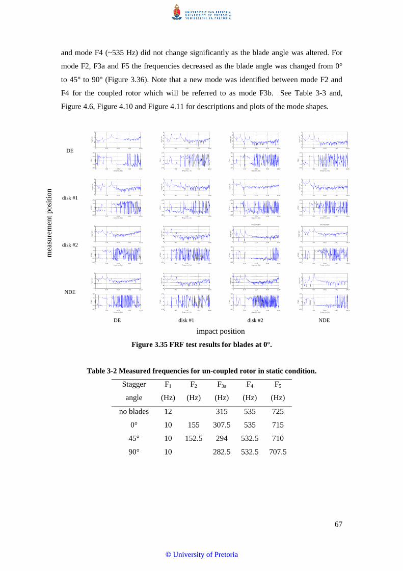
67

and mode F4 (~535 Hz) did not change significantly as the blade angle was altered. For

mode F2, F3a and F5 the frequencies decreased as the blade angle was changed from 0°

to 45° to 90° (Figure 3.36). Note that a new mode was identified between mode F2 and

F4 for the coupled rotor which will be referred to as mode F3b. See Table 3-3 and,

Figure 4.6, Figure 4.10 and Figure 4.11 for descriptions and plots of the mode shapes.

mea

sure

men

t p

osi

tio

n

DE

disk #1

disk #2

NDE

DE disk #1 disk #2 NDE

impact position

Figure 3.35 FRF test results for blades at 0°.

Table 3-2 Measured frequencies for un-coupled rotor in static condition.

Stagger

angle

F1

(Hz)

F2

(Hz)

F3a

(Hz)

F4

(Hz)

F5

(Hz)

no blades 12 315 535 725

0° 10 155 307.5 535 715

45° 10 152.5 294 532.5 710

90° 10 282.5 532.5 707.5


68

Figure 3.36 Measured frequency reduction vs. blade stagger angle (uncoupled, 0 rpm).

Table 3-3 Description of mode shapes.

Mode Description

Blades Shaft

F1 unknown unknown

F2 1st bending

(out of phase with rest of rotor)

all sections in phase

(low level of participation)

F3a 1st bending

(out of phase with disc #1) NDE coupling & disc #1 out of phase with disc #2 and #3

F3b 1st bending

(out of phase with disc #1)

armature & DE coupling

out of phase with disc #1 to #3

F4 1st bending

(low level of participation) disc #3

F5 2nd bending DE coupling

(exist only for uncoupled rotor)

3.5.4 Static modal testing of coupled rotor

Modal testing of the coupled rotor was conducted after assembling it in the test bench

(see Figure 3.2). The impact hammer, TLV and OR35 were used to conduct all tests with

measurement and impact positions the same as for the un-coupled rotor (i.e. 4x4 test

matrix, see section 3.5.2). A frequency range of 1 kHz was selected with 3201 lines to

give a frequency resolution of 312.5 mHz. Three spectral averages per test were taken. A

hammer trigger level of 1 N was used and a time delay of -1% or 32 ms. Force and

response windows were applied to the hammer and TLV signals.

Reciprocity was again clear from the results and to demonstrate this measurement/impact

position pairs DE/NDE and NDE/DE, for the blades mounted in the 0 degree position are

presented in Figure 3.37 and Figure 3.38. The effect of the telemetry system mass on the

natural frequencies of the test rotor was investigated by comparing the measured natural

90 deg 45 deg 0 deg no blades0

2

4

6

8

10

12

14

16

18

20

blade orientation

change in f

requency (

%)

F1

F2

F3a

F4

F5


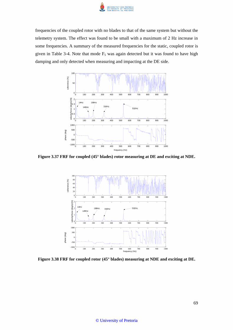
69

frequencies of the coupled rotor with no blades to that of the same system but without the

telemetry system. The effect was found to be small with a maximum of 2 Hz increase in

some frequencies. A summary of the measured frequencies for the static, coupled rotor is

given in Table 3-4. Note that mode F5 was again detected but it was found to have high

damping and only detected when measuring and impacting at the DE side.

Figure 3.37 FRF for coupled (45° blades) rotor measuring at DE and exciting at NDE.

Figure 3.38 FRF for coupled rotor (45° blades) measuring at NDE and exciting at DE.

0 100 200 300 400 500 600 700 800 900 10000

50

100

coh

ere

nce (

%)

0 100 200 300 400 500 600 700 800 900 10000

0.5

1

1.5

2

velo

city/f

orc

e (

de

g/s

)/(N

)

0 100 200 300 400 500 600 700 800 900 1000-1000

-500

0

500

1000

pha

se

(d

eg)

frequency (Hz)

14Hz

149Hz

198Hz

316Hz 532Hz

0 100 200 300 400 500 600 700 800 900 10000

20

40

60

80

100

coh

ere

nce (

%)

0 100 200 300 400 500 600 700 800 900 10000

1

2

3

velo

city/f

orc

e (

de

g/s

)/(N

)

0 100 200 300 400 500 600 700 800 900 1000-1000

-500

0

500

1000

pha

se

(d

eg)

frequency (Hz)

14Hz

149Hz

198Hz 316Hz 532Hz


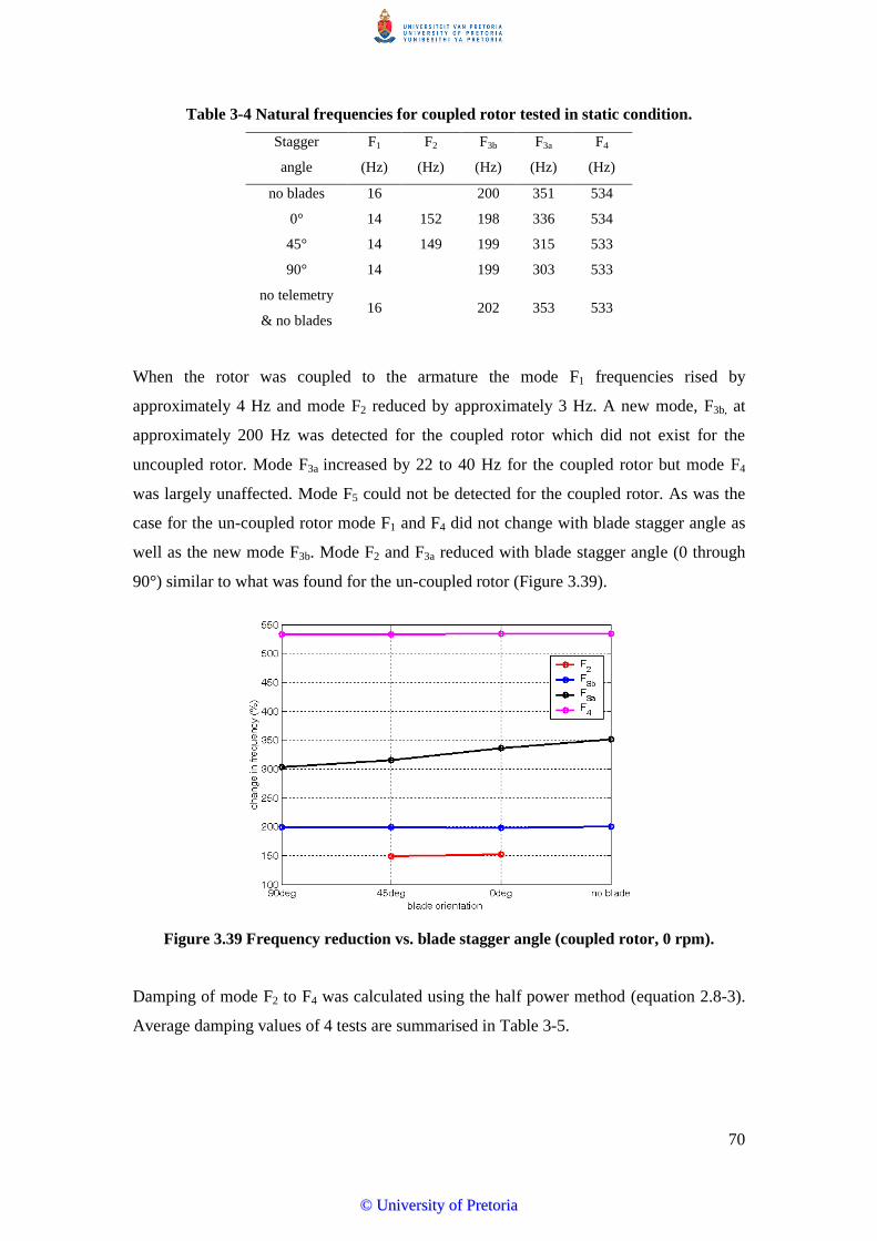
70

Table 3-4 Natural frequencies for coupled rotor tested in static condition.

Stagger

angle

F1

(Hz)

F2

(Hz)

F3b

(Hz)

F3a

(Hz)

F4

(Hz)

no blades 16 200 351 534

0° 14 152 198 336 534

45° 14 149 199 315 533

90° 14 199 303 533

no telemetry

& no blades 16 202 353 533

When the rotor was coupled to the armature the mode F1 frequencies rised by

approximately 4 Hz and mode F2 reduced by approximately 3 Hz. A new mode, F3b, at

approximately 200 Hz was detected for the coupled rotor which did not exist for the

uncoupled rotor. Mode F3a increased by 22 to 40 Hz for the coupled rotor but mode F4

was largely unaffected. Mode F5 could not be detected for the coupled rotor. As was the

case for the un-coupled rotor mode F1 and F4 did not change with blade stagger angle as

well as the new mode F3b. Mode F2 and F3a reduced with blade stagger angle (0 through

90°) similar to what was found for the un-coupled rotor (Figure 3.39).

Figure 3.39 Frequency reduction vs. blade stagger angle (coupled rotor, 0 rpm).

Damping of mode F2 to F4 was calculated using the half power method (equation 2.8-3).

Average damping values of 4 tests are summarised in Table 3-5.


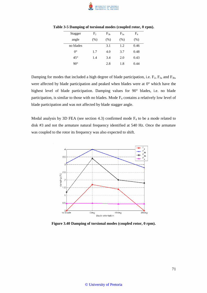
71

Table 3-5 Damping of torsional modes (coupled rotor, 0 rpm).

Stagger

angle

F2

(%)

F3b

(%)

F3a

(%)

F4

(%)

no blades 3.1 1.2 0.46

0° 1.7 4.0 3.7 0.48

45° 1.4 3.4 2.0 0.43

90° 2.8 1.8 0.44

Damping for modes that included a high degree of blade participation, i.e. F2, F3a and F3b,

were affected by blade participation and peaked when blades were at 0° which have the

highest level of blade participation. Damping values for 90° blades, i.e. no blade

participation, is similar to those with no blades. Mode F4 contains a relatively low level of

blade participation and was not affected by blade stagger angle.

Modal analysis by 3D FEA (see section 4.3) confirmed mode F4 to be a mode related to

disk #3 and not the armature natural frequency identified at 540 Hz. Once the armature

was coupled to the rotor its frequency was also expected to shift.

Figure 3.40 Damping of torsional modes (coupled rotor, 0 rpm).


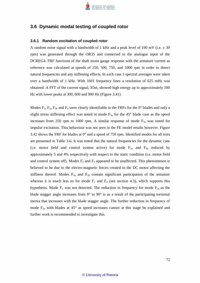
72

3.6 Dynamic modal testing of coupled rotor

3.6.1 Random excitation of coupled rotor

A random noise signal with a bandwidth of 1 kHz and a peak level of 100 mV (i.e. ± 30

rpm) was generated through the OR35 and connected to the analogue input of the

DCREG4. FRF functions of the shaft strain gauge response with the armature current as

reference was calculated at speeds of 250, 500, 750, and 1000 rpm in order to detect

natural frequencies and any stiffening effects. In each case 3 spectral averages were taken

over a bandwidth of 1 kHz. With 1601 frequency lines a resolution of 625 mHz was

obtained. A FFT of the current signal, IOut, showed high energy up to approximately 100

Hz with lower peaks at 300, 600 and 900 Hz (Figure 3.41).

Modes F2, F3a F3b and F4 were clearly identifiable in the FRFs for the 0° blades and only a

slight stress stiffening effect was noted in mode F3a for the 45° blade case as the speed

increases from 250 rpm to 1000 rpm. A similar response of mode F3a was noted for

impulse excitation. This behaviour was not seen in the FE model results however. Figure

3.42 shows the FRF for blades at 0° and a speed of 750 rpm. Identified modes for all tests

are presented in Table 3-6. It was noted that the natural frequencies for the dynamic case

(i.e. motor field and control system active) for mode F3a and F3b reduced by

approximately 5 and 4% respectively with respect to the static condition (i.e. motor field

and control system off). Modes F2 and F5 appeared to be unaffected. This phenomenon is

believed to be due to the electro-magnetic forces created in the DC motor affecting the

stiffness thereof. Modes F3a and F3b contain significant participation of the armature

whereas it is much less so for mode F2 and F4 (see section 4.3), which supports this

hypothesis. Mode F1 was not detected. The reduction in frequency for mode F3a as the

blade stagger angle increases from 0° to 90° is as a result of the participating torsional

inertia that increases with the blade stagger angle. The further reduction in frequency of

mode F3a with blades at 45° as speed increases cannot at this stage be explained and

further work is recommended to investigate this.


73

Figure 3.41 FFT of current signal (IOut) during random excitation.

Figure 3.42 FRF of strain gauge response with IOut as reference at 750 rpm.

0 100 200 300 400 500 600 700 800 900 10000

50

100

coh

ere

nce (

%)

0 100 200 300 400 500 600 700 800 900 10000

10

20

30

tors

ion/t

orq

ue

(V

/V)

0 100 200 300 400 500 600 700 800 900 1000-1000

-500

0

500

1000

pha

se

(d

eg)

frequency (Hz)

153.75Hz

191.25Hz 322.5Hz 531.25Hz


74

Table 3-6 Summary of results for random excitation of the coupled rotor.

speed

(rpm) F2 (Hz) F3b (Hz) F3a (Hz) F4 (Hz)

0 d

egre

e

250 151.88 190.00 320.00 530.63

500 151.25 189.38 323.75 531.88

750 153.75 191.25 322.50 531.25

1000 153.75 188.75 322.50 532.50

45

deg

ree

250 148.75 193.13 310.63 530.63

500 147.50 191.25 305.63 530.63

1000 148.75 191.50 302.50 530.00

90

deg

ree

250 188.75 293.13 530.63

500 184.38 292.50 531.25

750 187.50 293.13 530.00

1000 186.25 291.25 530.00

Figure 3.43 Frequency change vs. blade angle (coupled, random excitation, 250 rpm).

Similar to the static case, changes in blade stagger angle resulted in significant frequency

changes of mode F3a but less so for mode F2. Modes F3b and F4 were not affected.

Damping was calculated as a function of speed as well as blade stagger angle using the

half power method. Modes F3b and F4 are relatively well defined in the FRF plots. This

results in more reliable estimates of damping. Modes F2 and F3a are however not so well

defined in all cases which result in more randomness in the results. Damping of modes F2,

F3b and F4 tend to decrease with an increase in rotational speed. This was also noted for

90deg45deg0deg100

150

200

250

300

350

400

450

500

550

blade orientation

freq

uen

cy (

Hz)

F2

F3b

F3a

F4


75

mode F3a with blades at 0° but with blades at 45° and 90° this is not the case (Figure

3.44). Data suggests that damping under dynamic conditions also decreases with blade

stagger angle (0 through 90°), similar to static conditions, but poorly defined FRF peaks

for some modes may result in errors which show the opposite.

Figure 3.44 Damping vs. speed (coupled, random excitation).

Figure 3.45 Damping vs. blade stagger angle (coupled, random excitation).

3.6.2 Impulse excitation of coupled rotor

Using the function generator single short duration square waves were generated and

coupled to the analogue input of the DCREG4. This resulted in impulsive torque loading

of the rotor as can be seen in Figure 3.46. Using the motor current signal (IOut) as

reference the FRF of the strain gauge response was calculated.


76

Tests were conducted at mean speeds of 250, 500, 750 and 940 rpm with blades at 0, 45

and 90°. Five spectral averages were taken over a frequency range of 1 kHz and a

resolution of 625 mHz. Results were similar to those obtained through random excitation

except for mode F3b which was found to be 4% lower in the case of the impulse tests (see

Figure 3.49 to Figure 3.51). A slight speed dependency is noted for only mode F3a for 45°

blades similar to what was found for random excitation. The frequency of this mode

decreases with speed. Mode F1 was again not detected. The FRF for a mean speed of 940

rpm is shown in Figure 3.47 and all results are summarised in Table 3-7.

Figure 3.46 Response of rotor to impulsive torque loading.

Figure 3.47 FRF for impulsive loading at a mean speed of 940 rpm.

0 100 200 300 400 500 600 700 800 900 10000

50

100

coh

ere

nce (

%)

0 100 200 300 400 500 600 700 800 900 10000

10

20

30

tors

ion/t

orq

ue

(V

/V)

0 100 200 300 400 500 600 700 800 900 1000-1000

-500

0

500

1000

pha

se

(d

eg)

frequency (Hz)

153 Hz 325 Hz

530 Hz


77

Table 3-7 Summary of results for impulse excitation of the coupled rotor.

speed

(rpm) F2 (Hz) F3b (Hz) F3a (Hz) F4 (Hz)

0 d

egre

e

250 151.3 182.5 322.5 533.8

500 152.5 181.9 320.0 530.6

750 152.5 181.9 323.1 530.0

940 152.5 180.6 324.4 532.5

45

deg

ree 250 148.8 181.9 310.6 531.3

500 148.3 186.3 305.6 530.6

1000 150.0 176.3 302.5 530.6

90

deg

ree

250 183.8 298.8 530.0

500 172.5 297.5 531.9

750 178.8 286.8 528.9

940 180.0 290.0 528.8

Figure 3.48 Frequency reduction vs. blade angle (coupled, impulse excitation, 250 rpm).

NOTE: ran refers to random excitation shown for comparison and imp for impulse excitation.

The variation of frequency with blade stagger angle for impulse excitation is similar to

those found for random excitation (Figure 3.48).

Measured Campbell diagrams are shown in Figure 3.49 to Figure 3.51

90deg45 deg0deg100

150

200

250

300

350

400

450

500

550

freq

uen

cy (

Hz)

blade orientation

F2 ran

F3b

ran

F3a

ran

F4 ran

F2 imp

F3b

imp

F3a

imp

F4 imp


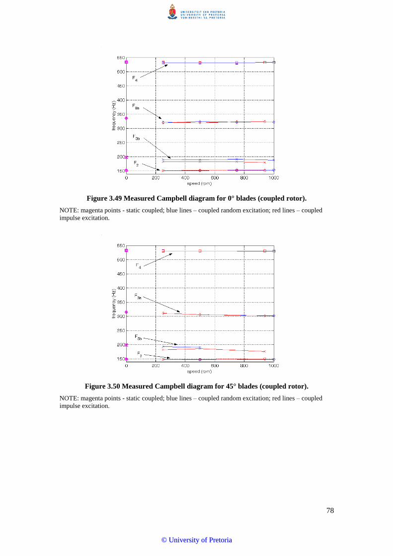
78

Figure 3.49 Measured Campbell diagram for 0° blades (coupled rotor).

NOTE: magenta points - static coupled; blue lines – coupled random excitation; red lines – coupled

impulse excitation.



impulse excitation.


79



impulse excitation.

Damping calculations using the half power method for the impulse excitation tests

resulted in similar values as for the random excitation tests for mode F3a and F4.

Randomness for mode F3b is expected to be due to poorly defined FRF peaks used for the

calculation of damping (Figure 3.52).

Figure 3.52 Damping vs. speed (coupled, impulse excitation).

3.6.3 Background noise

Waterfall plots of the shaft strain gauge response over the speed range 120 to 1000 rpm

were recorded at intervals of 5 rpm for blades in the 0, 45 and 90° positions as well as for

the rotor with no blades. No excitation was applied during these tests. Speed increments


80

were controlled via the OR35 output using a sine wave of 0 Hz frequency and

incrementing the output voltage by 20 mV to effect a ~5 rpm speed increase with each

step. A speed increment event was programmed and used as the FFT trigger. Three

spectral averages were calculated at each speed increment. The optical fibre switch was

used as a tachometer input to the OR35.

The plot with blades at 0° clearly show mode F4 at 534 Hz. ‘Activity’ around 150Hz

could be interpreted as either mode F2 or a multiple of line frequency. Based on the fact

that much less ‘activity’ is seen in the case of 90° blades and with no blades, which do not

contain mode F2, it is concluded that mode F2 is detected for the 0 and 45 ° case. A strong

response is seen at 200 Hz which is likely to be a multiple of line frequency as mode F3b

is expected to be closer to 190 Hz based on the random excitation and impulse tests. The

control system frequency at 300 Hz is very dominant as well as the 2nd harmonic thereof

at 600 Hz. Mode F1 at ~14 Hz could not be identified in this test. Excitation lines which

are multiples of running speed emanates from the zero point radially outwards. Sidebands

around 300 and 600 Hz can be clearly seen.

Figure 3.53 Waterfall plot for blades at 0° (coupled rotor).


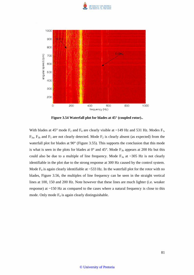
81

Figure 3.54 Waterfall plot for blades at 45° (coupled rotor)..

With blades at 45° mode F2 and F4 are clearly visible at ~149 Hz and 531 Hz. Modes F1,

F3a, F3b and F5 are not clearly detected. Mode F2 is clearly absent (as expected) from the

waterfall plot for blades at 90° (Figure 3.55). This supports the conclusion that this mode

is what is seen in the plots for blades at 0° and 45°. Mode F3b appears at 200 Hz but this

could also be due to a multiple of line frequency. Mode F3a at ~305 Hz is not clearly

identifiable in the plot due to the strong response at 300 Hz caused by the control system.

Mode F4 is again clearly identifiable at ~533 Hz. In the waterfall plot for the rotor with no

blades, Figure 3.56, the multiples of line frequency can be seen in the straight vertical

lines at 100, 150 and 200 Hz. Note however that these lines are much lighter (i.e. weaker

response) at ~150 Hz as compared to the cases where a natural frequency is close to this

mode. Only mode F4 is again clearly distinguishable.


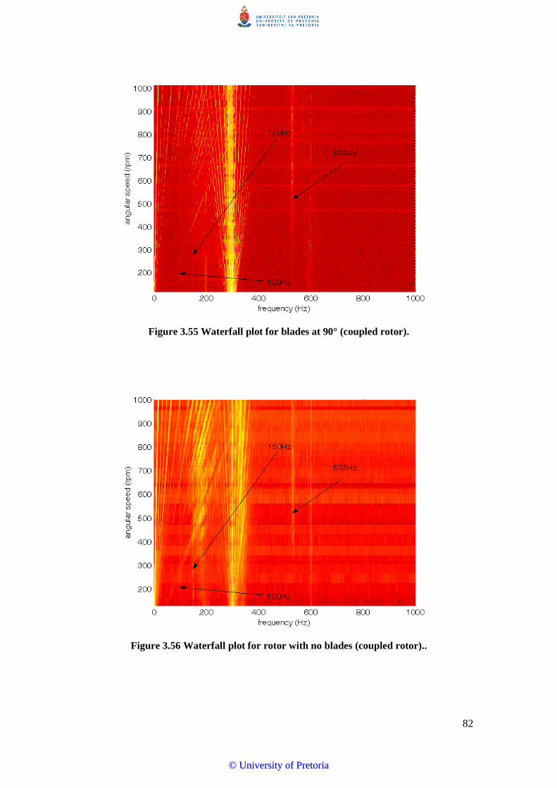
82

Figure 3.55 Waterfall plot for blades at 90° (coupled rotor).

Figure 3.56 Waterfall plot for rotor with no blades (coupled rotor)..


83

3.7 Blade response

Using the strain gauge bridge mounted on blade #8 the response of this blade to free

running, random excitation and impulse loading was measured to obtain the frequency

response thereof. Tests were conducted for blades at 0° and 45 °.

3.7.1 Background noise

FFTs of the blade response were measured with the rotor running at constant speeds of

250, 500, 750 and 1000 rpm. Ten spectral averages were taken with a frequency

bandwidth of 1 kHz and a resolution of 625 mHz.

In all cases 1x running speed is clearly visible as well as the 300 and 600 Hz peak due to

the control system forcing at this frequency. The first and second bending modes of blade

#8 at ~145 and ~896 Hz can be seen in Figure 3.57. In addition the response of rigid shaft

modes at ~152 (1st bending, F2) and ~ 902 Hz (2nd bending) were also detected. The

torsional mode F3a at ~320 Hz is also distinguishable. No significant stress stiffening over

the measured speed range was observed.

Figure 3.57 FFT of blade strain gauge response at 250 rpm (0° blades).

A waterfall plot of the blade strain gauge response for the speed range 120 to 1000 rpm is

shown in Figure 3.58. Blade #8’s first and second mode is distinguishable at ~145 and

896 Hz respectively. An additional frequency, expected to be a rigid shaft mode with the

2nd bending mode of the blades, can be seen at ~930 Hz.


84

Figure 3.58 Waterfall plot of blade strain gauge response (0° blades).

3.7.2 Blade response to random excitation

The same setup for random excitation as described in section 3.6.1 is applied with blades

at 0°. The same results were obtained as in the waterfall plots except that mode F3a was

also detected.

Figure 3.59 Blade response with random excitation (0°, 250 rpm).

0 100 200 300 400 500 600 700 800 900 10000

50

100

coh

ere

nce (

%)

0 100 200 300 400 500 600 700 800 900 10000

50

100

150

200

ben

din

g s

tre

ss/

torq

ue

(V

/V)

0 100 200 300 400 500 600 700 800 900 1000-1000

-500

0

500

1000

pha

se

(d

eg)

frequency

145Hz 151.25Hz

325.5Hz

896Hz 935Hz


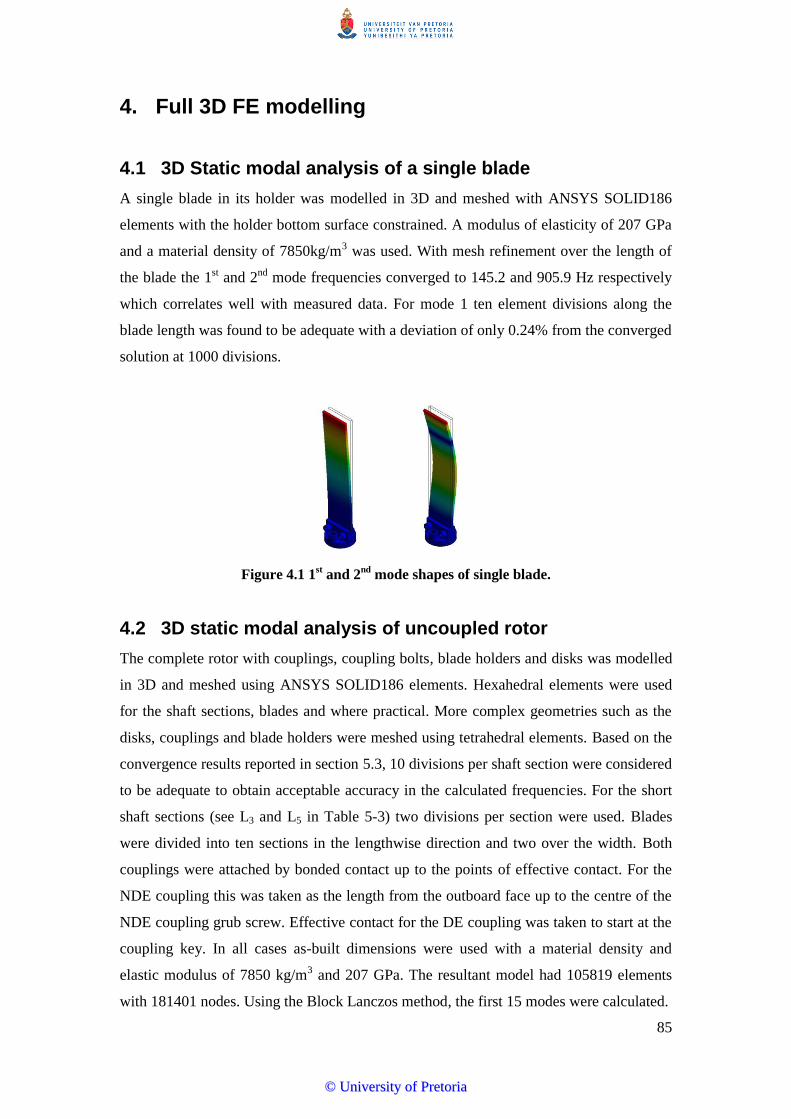
85

4. Full 3D FE modelling

4.1 3D Static modal analysis of a single blade

A single blade in its holder was modelled in 3D and meshed with ANSYS SOLID186

elements with the holder bottom surface constrained. A modulus of elasticity of 207 GPa

and a material density of 7850kg/m3 was used. With mesh refinement over the length of

the blade the 1st and 2nd mode frequencies converged to 145.2 and 905.9 Hz respectively

which correlates well with measured data. For mode 1 ten element divisions along the

blade length was found to be adequate with a deviation of only 0.24% from the converged

solution at 1000 divisions.

Figure 4.1 1st and 2

nd mode shapes of single blade.

4.2 3D static modal analysis of uncoupled rotor

The complete rotor with couplings, coupling bolts, blade holders and disks was modelled

in 3D and meshed using ANSYS SOLID186 elements. Hexahedral elements were used

for the shaft sections, blades and where practical. More complex geometries such as the

disks, couplings and blade holders were meshed using tetrahedral elements. Based on the

convergence results reported in section 5.3, 10 divisions per shaft section were considered

to be adequate to obtain acceptable accuracy in the calculated frequencies. For the short

shaft sections (see L3 and L5 in Table 5-3) two divisions per section were used. Blades

were divided into ten sections in the lengthwise direction and two over the width. Both

couplings were attached by bonded contact up to the points of effective contact. For the

NDE coupling this was taken as the length from the outboard face up to the centre of the

NDE coupling grub screw. Effective contact for the DE coupling was taken to start at the

coupling key. In all cases as-built dimensions were used with a material density and

elastic modulus of 7850 kg/m3 and 207 GPa. The resultant model had 105819 elements

with 181401 nodes. Using the Block Lanczos method, the first 15 modes were calculated.


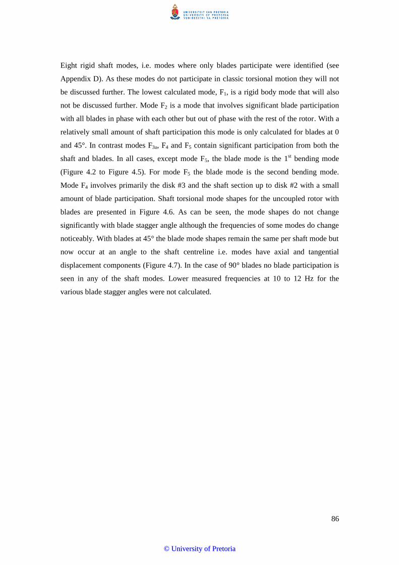
86

Eight rigid shaft modes, i.e. modes where only blades participate were identified (see

Appendix D). As these modes do not participate in classic torsional motion they will not

be discussed further. The lowest calculated mode, F1, is a rigid body mode that will also

not be discussed further. Mode F2 is a mode that involves significant blade participation

with all blades in phase with each other but out of phase with the rest of the rotor. With a

relatively small amount of shaft participation this mode is only calculated for blades at 0

and 45°. In contrast modes F3a, F4 and F5 contain significant participation from both the

shaft and blades. In all cases, except mode F5, the blade mode is the 1st bending mode

(Figure 4.2 to Figure 4.5). For mode F5 the blade mode is the second bending mode.

Mode F4 involves primarily the disk #3 and the shaft section up to disk #2 with a small

amount of blade participation. Shaft torsional mode shapes for the uncoupled rotor with

blades are presented in Figure 4.6. As can be seen, the mode shapes do not change

significantly with blade stagger angle although the frequencies of some modes do change

noticeably. With blades at 45° the blade mode shapes remain the same per shaft mode but

now occur at an angle to the shaft centreline i.e. modes have axial and tangential

displacement components (Figure 4.7). In the case of 90° blades no blade participation is

seen in any of the shaft modes. Lower measured frequencies at 10 to 12 Hz for the

various blade stagger angles were not calculated.


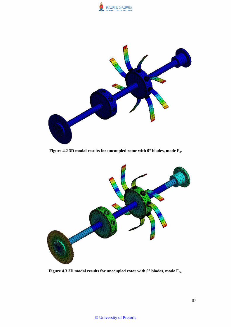
87

Figure 4.2 3D modal results for uncoupled rotor with 0° blades, mode F2.

Figure 4.3 3D modal results for uncoupled rotor with 0° blades, mode F3a.


88



Results for all blade stagger angles are shown in Table 4-1 and the errors relative to the

measured frequencies are given in Table 4-2.


89

Figure 4.6 Shaft mode-shapes for uncoupled rotor (3D FEA).

Figure 4.7 Mode F2 for uncoupled rotor with blades at 45°.


90

Table 4-1 Summary of 3D modelling results for the uncoupled rotor.

Stagger angle F2 (Hz) F3a (Hz) F4 (Hz) F5 (Hz)

no blades - 313.0 534.1 723.0

0° 153.8 304.9 533.1 713.1

45° 150.02 291.2 533.3 708.7

90° - 280.7 533.0 705.6

Table 4-2 Summary of % error in 3D modelling results for the uncoupled rotor.

Stagger angle F2 (%) F3a (%) F4 (%) F5 (%)

no blades -0.6 -0.2 -0.3

0° -0.8 -0.8 -0.4 -0.3

45° -1.6 -1.0 0.1 0.2

90° -0.6 0.1 -0.3

4.3 3D Static modal analysis of coupled rotor

Using the uncoupled model as a basis, the 3D model was extended to include the motor

armature as well as the motor coupling and coupling bolts (Figure 4.8). The shaft sections

of the armature were modelled as steel sections with an elastic modulus and density of

207 GPa and 7850 kg/m3. For the larger diameter winding section which has a complex

construction of a steel base, copper windings and laminated plates, the density and

stiffness were calibrated to represent the measured total armature polar moment of inertia

and to minimise the difference between the calculated and measured frequencies. Coupled

rotor frequencies for a range of densities and elastic moduli were calculated by 3D FEA

and a composite error index was defined as the average of the absolute differences

between the calculated and measured frequencies. Minimisation of the error index will

lead to the optimum density and elastic modulus values to be used in the model for the

armature to ensure the best correlation of all the calculated frequencies with that of the

measured frequencies. A surface plot of this error index is shown in Figure 4.9. The

absolute minimum error (0.43 %) was calculated to occur at a density of ~4600 kg/m3 and

an elastic modulus of 6.6 GPa. However, to ensure the modelled polar moment of inertia

is equal to the measured value a density of 3855.5 kg/m3 was used. Based on this density

the minimum error index occurs for an elastic modulus of 4.3 GPa, which was applied

throughout. Meshing of the complete coupled model resulted in 71016 elements and

131282 nodes.


91

Modes F2, F3a and F4 were again calculated as for the uncoupled case. Mode F5 was also

calculated but based on the fact that it is the 2nd blade bending mode, which is less likely

to be problematic in real systems, it is not considered further. A new mode, F3b, was

calculated at 198 Hz for the blades at 0°. This mode contains significant blade as well as

armature participation. Calculated shaft mode shapes are depicted in Figure 4.10 and 3D

model plots of the mode shapes are shown in Figure 4.11 to Figure 4.14. For all cases (F2,

F3a, F3b and F4) the blade tip movement is out of phase with that of disk #1 (disk blades

are mounted on) and the blade mode shape is confirmed to be the 1st bending mode as for

the uncoupled case.

Figure 4.8 Full 3D model of coupled rotor with blades at 0°.


92

Figure 4.9 Surface plot of composite error index.

For mode F3b the armature and DE coupling is out of phase with the three disks. In mode

F3a the DE coupling and disk #1 is in phase but the pair is out of phase with the armature

and disk #2 and #3. Mode F4 involves primarily participation of disk #3 and the section of

shaft up to disk #2.

Other modes with no shaft participation i.e. only involving blades out of phase with each

other, so called rigid shaft modes, were also calculated but are not reported here.

Figure 4.10 Shaft mode shapes for coupled rotor (3D FEA).

0 0.2 0.4 0.6 0.8 1 1.2 1.4

-0.5

0

0.5

1

normalised shaft length

no

rmal

ised

to

rsio

nal

dis

pla

cem

ent

geometry

F2 0deg

F3b

0deg

F3a

0deg

F4 0deg

F2 45deg

F3b

45deg

F3a

45deg

F4 45deg

F3b

90deg

F3a

90deg

F4 90deg


93

Calculated frequencies for the 1st 4 modes of the coupled rotor with blades at 0, 45 and

90° and with no blades are summarised in Table 4-3with the associated error relative to

the measured values given in Table 4-4.

Figure 4.11 Coupled rotor model mode shape plots for 3D modal analysis, mode F2.

Figure 4.12 Coupled rotor model mode shape plots for 3D modal analysis, mode F3b.


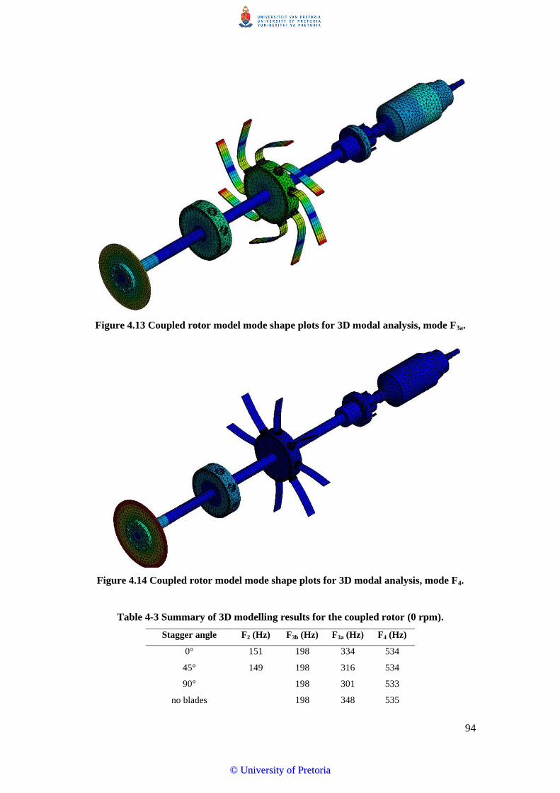
94

Figure 4.13 Coupled rotor model mode shape plots for 3D modal analysis, mode F3a.

Figure 4.14 Coupled rotor model mode shape plots for 3D modal analysis, mode F4.

Table 4-3 Summary of 3D modelling results for the coupled rotor (0 rpm).

Stagger angle F2 (Hz) F3b (Hz) F3a (Hz) F4 (Hz)

0° 151 198 334 534

45° 149 198 316 534

90° 198 301 533

no blades 198 348 535


95

Table 4-4 Summary of % error of 3D modelling for the coupled rotor (0 rpm).

Stagger angle F2 (%) F3 (%) F4 (%) F5 (%)

0° -0.7% 0.2% -0.6% 0.0%

45° -0.1% -0.5% 0.2% 0.1%

90° -0.7% -0.5% 0.1%

no blades -0.9% -0.8% 0.1%

Solution time for the full 3D static modal analysis was found to be approximately 100

seconds.

4.4 3D dynamic modal analysis of coupled rotor

A pre-stress modal analysis of the coupled rotor with blades at 0, 45 and 90 degrees was

done for speeds ranging from 0 to 6000 rpm using the same models as discussed in the

previous section. Although the maximum tested speed was only up to 1000 rpm (for

safety reasons), calculations were done up to the higher speed to show that some modes

are affected by centrifugal stiffening. The Campbell diagram based on the armature

winding section elastic modulus that was obtained after optimisation with respect to static

conditions showed good correlation with mode F2 and F4. As reported in section 3.6.1

dynamic frequencies of mode F3a and F3b reduce relative to the static condition and it was

hypothesized to be due to electro-magnetic effects on the motor armature that reduce the

stiffness thereof. To compensate for this the elastic modulus of the winding section of the

armature was again calibrated to optimize the zero rpm frequencies of mode F3a and F3b

(for 0° blades). An elastic modulus of 3.2 GPa was calculated which resulted in an

improved fit to the experimental data for mode F3a and F3b whilst mode F2 and F4 were

unaffected by the lower value (Figure 4.15).

Calculations confirm that torsional frequencies are only affected by rotational speed from

approximately 2000 rpm. Modes F3b and F4 appear to be unaffected by speed (except for

possible loci veering at around 5000 rpm). A consistent non-linear speed dependency is

seen for modes F2 and F3a.


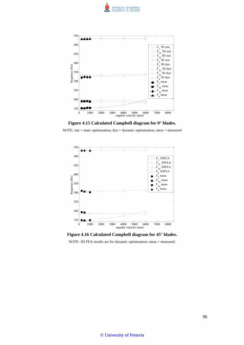
96

Figure 4.15 Calculated Campbell diagram for 0° blades.

NOTE: stat = static optimisation; dyn = dynamic optimisation; meas = measured


NOTE: 3D FEA results are for dynamic optimisation; meas = measured.

0 1000 2000 3000 4000 5000 6000 7000 8000

150

200

250

300

350

400

450

500

550

angular velocity (rpm)

frequency

(H

z)

F2 3D stat

F3b

3D stat

F3a

3D stat

F4 3D stat

F2 3D dyn

F3b

3D dyn

F3a

3D dyn

F4 3D dyn

F2 meas

F3b

meas

F3a

meas

F4 meas

0 1000 2000 3000 4000 5000 6000 7000 8000

150

200

250

300

350

400

450

500

550


frequency

(H

z)

F2 3DFEA

F3b

3DFEA

F3a

3DFEA

F4 3DFEA

F2 meas

F3b

meas

F3a

meas

F4 meas


97


NOTE: 3D FEA results are for dynamic optimisation; meas = measured.

Figure 4.18 Frequency reduction vs. blade angle (coupled, full 3D, 1000 rpm).

NOTE: ran refers to random excitation shown for comparison; 3D FEA results are for dynamic

optimisation; meas = measured.

Frequency dependence on blade stagger angle calculated by full 3D analysis for dynamic

conditions correlated well with measured data (Figure 4.18).

Solution time per-stressed modal analysis point was found to be in the range of 110

seconds.

0 1000 2000 3000 4000 5000 6000 7000 8000

150

200

250

300

350

400

450

500

550


frequency

(H

z)

F3b

3DFEA

F3a

3DFEA

F4 3DFEA

F3b

meas

F3a

meas

F4 meas

0deg 45deg 90deg100

150

200

250

300

350

400

450

500

550

frequency

(H

z)

blade orientation

F2 3DFEA

F3b

3DFEA

F3a

3DFEA

F4 3DFEA

F2 meas

F3b

meas

F3a

meas

F4 meas


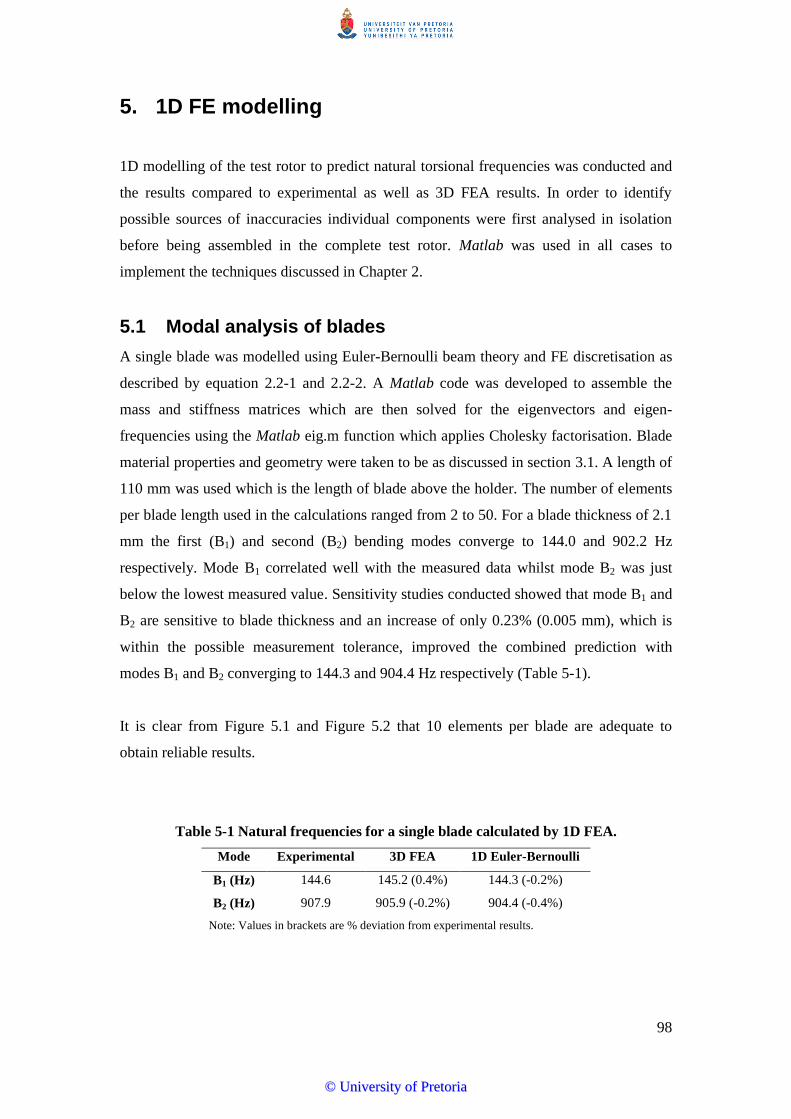
98

5. 1D FE modelling

1D modelling of the test rotor to predict natural torsional frequencies was conducted and

the results compared to experimental as well as 3D FEA results. In order to identify

possible sources of inaccuracies individual components were first analysed in isolation

before being assembled in the complete test rotor. Matlab was used in all cases to

implement the techniques discussed in Chapter 2.

5.1 Modal analysis of blades

A single blade was modelled using Euler-Bernoulli beam theory and FE discretisation as

described by equation 2.2-1 and 2.2-2. A Matlab code was developed to assemble the

mass and stiffness matrices which are then solved for the eigenvectors and eigen-

frequencies using the Matlab eig.m function which applies Cholesky factorisation. Blade

material properties and geometry were taken to be as discussed in section 3.1. A length of

110 mm was used which is the length of blade above the holder. The number of elements

per blade length used in the calculations ranged from 2 to 50. For a blade thickness of 2.1

mm the first (B1) and second (B2) bending modes converge to 144.0 and 902.2 Hz

respectively. Mode B1 correlated well with the measured data whilst mode B2 was just

below the lowest measured value. Sensitivity studies conducted showed that mode B1 and

B2 are sensitive to blade thickness and an increase of only 0.23% (0.005 mm), which is

within the possible measurement tolerance, improved the combined prediction with

modes B1 and B2 converging to 144.3 and 904.4 Hz respectively (Table 5-1).

It is clear from Figure 5.1 and Figure 5.2 that 10 elements per blade are adequate to

obtain reliable results.

Table 5-1 Natural frequencies for a single blade calculated by 1D FEA.

Mode Experimental 3D FEA 1D Euler-Bernoulli

B1 (Hz) 144.6 145.2 (0.4%) 144.3 (-0.2%)

B2 (Hz) 907.9 905.9 (-0.2%) 904.4 (-0.4%)

Note: Values in brackets are % deviation from experimental results.


99

Figure 5.1 Convergence of blade mode B1.

Figure 5.2 Convergence of blade mode B2.

5.2 Shaft only analysis

The shaft only with no disks and in the free-free condition was modelled (equation 2.3-1

and 2.3-2) and results compared to full 3D analysis conducted in ANSYS. A distributed

parameter approach was used with each section of shaft divided into the same number of

divisions which is increased until convergence is reached. A required convergence level

0.1% was applied. Note that no compensation was made for changes in diameter as these

are small and the effect found to be negligible. Good agreement was found between the

1D approach and full 3D FEA (Table 5-2).


100

Table 5-2 Torsional frequencies for ‘shaft only’ 1D analyses.

Mode 3D FEA 1D FEA

S1 (Hz) 1950.2 1950.5 (0.02%)

S2 (Hz) 3610.6 3611.6 (0.03%)

S3 (Hz) 5386.1 5386.8 (0.01%)

Note: Values in brackets are % deviation from

3D FEA results.

It was found that at least 20 elements per shaft section results in acceptably converged

frequencies (Figure 5.3).

Figure 5.3 1D FE convergence of ‘shaft only’ frequencies .

5.3 Shaft with disks

Natural frequencies for the shaft with disks #1 and #2 mounted were calculated and

compared to full 3D FEA results. The shaft is modelled as 7 separate sections (see Figure

5.4) with lumped inertias (J2 and J3) added at the end of shaft section L3 and L4 to account

for the disks. The disk moment of inertia was obtained from the 3D solid model and

found to be 0.0142 kg.m2. Disks are assumed to be integral to the shaft.


101

Figure 5.4 Line diagram of shaft with disks.

With no compensation for the sudden diameter changes at the shaft/disk interfaces the

difference between the 1D and the 3D FEA approach was found to be 2.4, 1.4 and 1.4%

for the 1st three modes respectively (Figure 5.5).

Figure 5.5 Convergence for 1D shaft-disk system with no diameter compensation.

Based on the 3D FEA extended BICERA approach (Figure 2.3) a sudden diameter change

compensation factor of 15.7% was determined. The smaller and larger diameters ( and

( ) were taken as the shaft and disk diameters respectively. A radius ( ) between the

disk and shaft interface of 0 mm was assumed. Compensation for sudden diameter change

between shaft sections 3 and 4 and disk #2 as well as between sections 4 and 5 and disk

#1 was required. With compensation the difference between the 1D and 3D FE calculated

frequencies decreased to less than 0.2% for all modes (Figure 5.6).


102

Figure 5.6 Convergence for 1D shaft-disk system with compensation for sudden

diameter change.

5.4 Uncoupled rotor 1D modelling

The 1D model of the complete rotor, uncoupled from the motor armature, with no blades

may be represented by a line diagram as in Figure 5.7. J1 to J4 represent the lumped

inertias of the NDE coupling, disk #2, disk #1 and the DE coupling respectively. C1 to C4

represent added virtual shaft lengths to compensate for sudden diameter changes and L1

to L7 represent real shaft lengths. Note that virtual shaft lengths are added to real shaft

lengths with the same number (i.e. L1=L1+C1) for the discretisation of the model. Based

on the convergence results of section 5.3, 20 divisions per shaft section were used from

this point forward. Values of the lumped inertias for the complete disk and coupling

geometries were obtained from the 3D models thereof. All dimensions were based on

measured dimensions of the as built rotor (see Table 5-3 for a summary of variables

used). Sudden diameter change compensation factors of 26 and 18% (based on shaft

diameter) were determined by 3D FEA for the NDE and DE couplings respectively. This

was required as the geometry of these interfaces (overhang of non-contact lengths of

couplings) proved not to follow the same behaviour as for sudden diameter changes as

captured by Figure 2.3.


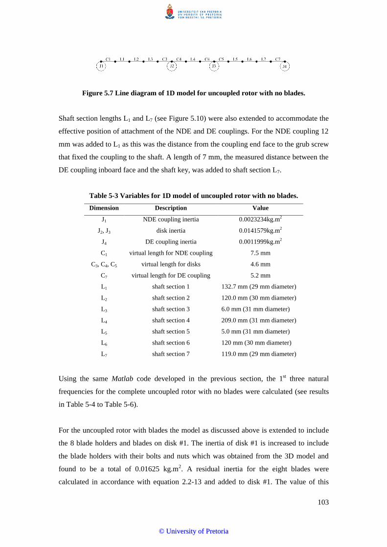
103

Figure 5.7 Line diagram of 1D model for uncoupled rotor with no blades.

Shaft section lengths L1 and L7 (see Figure 5.10) were also extended to accommodate the

effective position of attachment of the NDE and DE couplings. For the NDE coupling 12

mm was added to L1 as this was the distance from the coupling end face to the grub screw

that fixed the coupling to the shaft. A length of 7 mm, the measured distance between the

DE coupling inboard face and the shaft key, was added to shaft section L7.

Table 5-3 Variables for 1D model of uncoupled rotor with no blades.

Dimension Description Value

J1 NDE coupling inertia 0.0023234kg.m2

J2, J3 disk inertia 0.0141579kg.m2

J4 DE coupling inertia 0.0011999kg.m2

C1 virtual length for NDE coupling 7.5 mm

C3, C4, C5 virtual length for disks 4.6 mm

C7 virtual length for DE coupling 5.2 mm

L1 shaft section 1 132.7 mm (29 mm diameter)





L6 shaft section 6 120 mm (30 mm diameter)


Using the same Matlab code developed in the previous section, the 1st three natural

frequencies for the complete uncoupled rotor with no blades were calculated (see results

in Table 5-4 to Table 5-6).

For the uncoupled rotor with blades the model as discussed above is extended to include

the 8 blade holders and blades on disk #1. The inertia of disk #1 is increased to include

the blade holders with their bolts and nuts which was obtained from the 3D model and

found to be a total of 0.01625 kg.m2. A residual inertia for the eight blades were

calculated in accordance with equation 2.2-13 and added to disk #1. The value of this


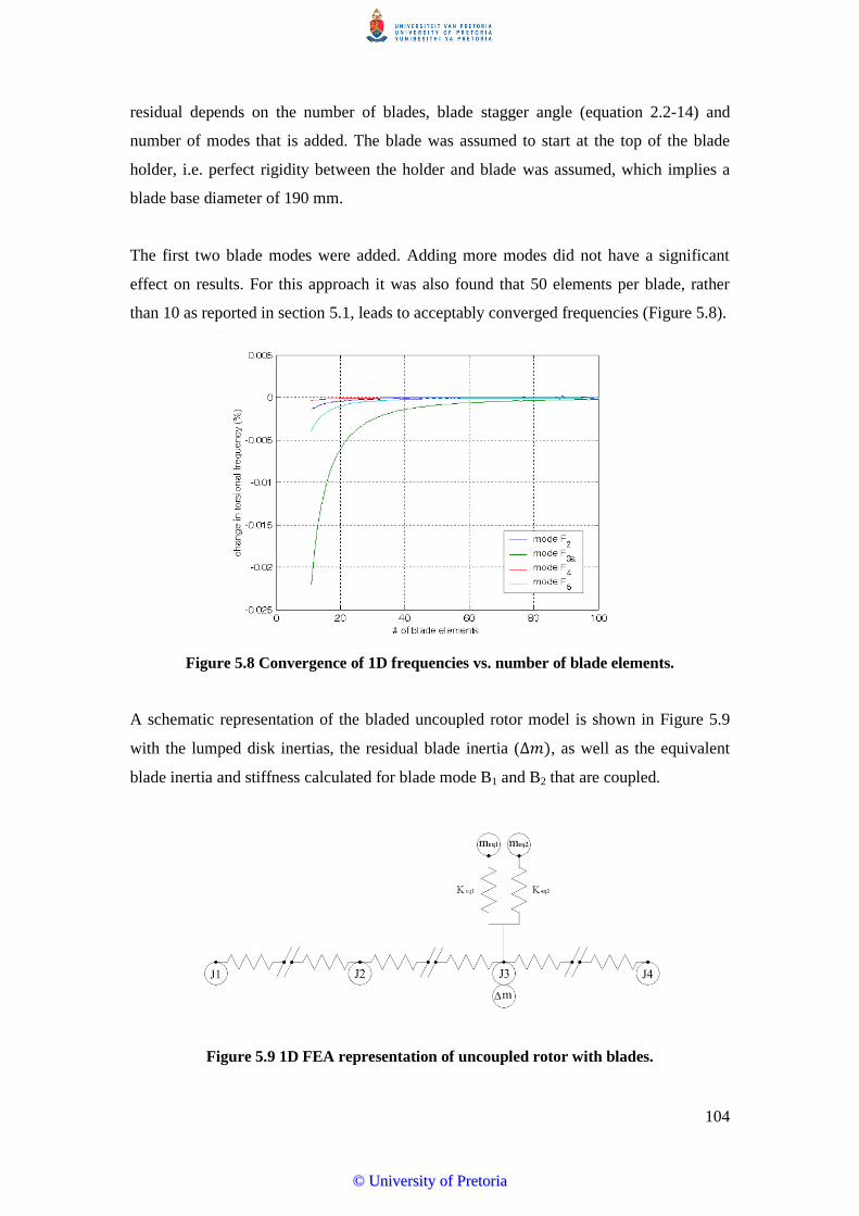
104

residual depends on the number of blades, blade stagger angle (equation 2.2-14) and

number of modes that is added. The blade was assumed to start at the top of the blade

holder, i.e. perfect rigidity between the holder and blade was assumed, which implies a

blade base diameter of 190 mm.

The first two blade modes were added. Adding more modes did not have a significant

effect on results. For this approach it was also found that 50 elements per blade, rather

than 10 as reported in section 5.1, leads to acceptably converged frequencies (Figure 5.8).

Figure 5.8 Convergence of 1D frequencies vs. number of blade elements.

A schematic representation of the bladed uncoupled rotor model is shown in Figure 5.9

with the lumped disk inertias, the residual blade inertia ( , as well as the equivalent

blade inertia and stiffness calculated for blade mode B1 and B2 that are coupled.

Figure 5.9 1D FEA representation of uncoupled rotor with blades.


105

Good correlation (< 1% error) with experimental results was obtained except for mode F2

with blades at 45° which has an error of 1.9% (Table 5-5). Good correlation was found

with full 3D FEA results (Table 5-6).

Table 5-4 Calculated frequencies for uncoupled rotor using 1D FEA.

Stagger angle F2 (Hz) F3a (Hz) F4 (Hz) F5 (Hz)

no blades - 313.1 533.9 723.8

0° 154.0 305.1 533.5 714.6

45° 149.6 291.7 533.2 711.3

90° - 281.4 532.9 708.6

Table 5-5 Error in 1D frequencies relative to experimental results.


no blades -0.6% -0.2% -0.2%

0° -0.7% -0.8% -0.3% -0.1%

45° -1.9% -0.8% 0.1% 0.2%

90° -0.4% 0.1% 0.2%

Table 5-6 Error in 1D frequencies relative to 3D results.


no blades 0.0% 0.0% 0.1%

0° 0.1% 0.1% 0.1% 0.2%

45° -0.3% 0.2% 0.0% 0.4%

90° 0.2% 0.0% 0.4%

5.5 Coupled rotor 1D modelling

For the rotor coupled to the armature the uncoupled 1D model was extended to include

the motor coupling and armature. Inertia J4 was increased to include inertia of the motor

coupling with its bolts and nuts.

Using as built dimensions the armature was modelled as a number of shaft sections (see

Figure 5.10 and Table 5-7). For the DE and NDE steel shaft sections, stiffness and inertia

was based on actual material properties. For the central winding and commutator areas

the equivalent density and elastic modulus as used in full 3D FEA (section 4.2) was


106

applied. Developed Matlab code BICERA.m was used to calculate compensation factors

for all sudden shaft diameter changes.

Figure 5.10 Definition of 1D shaft sections.

Table 5-7. Additional variables for 1D model of coupled rotor.

Dimension Description Value

L8 virtual shaft section 8 0.0023234kg.m2

L9 shaft section 9 0.0141579kg.m2

L10 shaft section 10 0.0011999kg.m2

L11 shaft section 11 7.5 mm








L19 shaft section 19 120 mm (30 mm diameter)

For the case where 2 blade modes are coupled the variation of the equivalent mode inertia

and the residual inertia with blade stagger angle is presented in Figure 5.11. The

equivalent inertia contribution from the first bending mode is significantly more than that

for the second bending mode except for stagger angles close to 90°. As expected the

equivalent tangential inertias for a stagger angle of 90° is zero as no blade participation

occurs in this case.


107

Figure 5.11 Equivalent inertia for coupled blade modes.

The calculated frequencies (Table 5-8) for all the cases investigated correlates well with

experimental results (Table 5-9) as well as with 3D FEA results (Table 5-10). Frequency

change with blade stagger angle is shown in Figure 5.12. Mode shape diagrams for the

investigated cases are shown in Figure 5.13. Participation of the blade modes B1 and B2

(1st and 2nd bending) in the shaft mode is indicated by the diamond and square data points.

The distance of the data point from the attachment node (disk #1) is an indication of the

level of participation of the blade mode relative to the rest of the rotor as per equation

2.4-1.

Good correlation is obtained between measured, full 3D and 1D frequency dependence on

blade stagger angle for static conditions (Figure 5.12).

Table 5-8 Calculated frequencies for coupled rotor using 1D approach.


no blades 197.4 347.5 534.9

0° 151.4 197.6 333.3 534.1

45° 148.4 197.2 315.3 533.6

90° 196.8 301.3 533.3


108

Table 5-9 Coupled rotor, error in 1D frequencies relative to experimental results.

Stagger angle F2 (%) F3b (%) F3a (%) F4 (%)

no blades -1.3% -1.0% 0.2%

0° -0.4% -0.2% -0.8% 0.0%

45° -0.4% -0.9% 0.1% 0.1%

90° -1.1% -0.6% 0.0%

Table 5-10 Coupled rotor, error in 1D frequencies relative to 3D FEA results.


no blades -0.3% -0.1% 0.0%

0° 0.2% -0.2% -0.2% 0.0%

45° -0.4% -0.4% -0.2% -0.1%

90° -0.6% 0.1% 0.0%

Figure 5.12 Frequency reduction vs. blade angle (coupled, 1D, 0 rpm).

NOTE: stat refers to measured data, 3D for full 3D analysis and 1D for 1D FE analysis.

90deg45deg0degno blade100

150

200

250

300

350

400

450

500

550

freq

uen

cy (

Hz)

blade orientation

F2 stat

F3b

stat

F3a

stat

F4 stat

F2 3D

F3b

3D

F3a

3D

F4 3D

F2 1D

F3b

1D

F3a

1D

F4 1D


109

(a) no blades (b) 0 °blades

(c) 45° blades (d) 90° blades

Figure 5.13 Mode shapes of coupled rotor using 1D analysis.

Solution times for the 1D static modal analysis was found to be in the order of 0.3

seconds.

0 0.2 0.4 0.6 0.8 1-1

-0.5

0

0.5

1

1.5


no

rmal

ised

to

rsio

nal

dis

pla

cem

ent

mode F3b

mode F3a

F4

blade mode/s

0 0.2 0.4 0.6 0.8 1-1

-0.5

0

0.5

1

1.5


no

rmal

ised

to

rsio

nal

dis

pla

cem

ent

mode F2

mode F3b

mode F3a

mode F4

0 0.2 0.4 0.6 0.8 1-1

-0.5

0

0.5

1

1.5


no

rmal

ised

to

rsio

nal

dis

pla

cem

ent

0 0.2 0.4 0.6 0.8 1-1

-0.5

0

0.5

1

1.5


no

rmal

ised

to

rsio

nal

dis

pla

cem

ent

mode F2

mode F3b

mode F3a

F4

lumped inertia

blade mode/s


110

6. 3D cyclic symmetric modelling

6.1 Coupled rotor 3DCS static modal analysis

Cyclic symmetric models for each of the coupled rotor cases described in the previous

sections were developed. In order to capture one of the eight blades the models consisted

of a 45° segment of the complete rotor maintaining all geometry features and including

one blade. The only notable difference is the number of DE coupling bolts. One bolt and

nut were included in the cyclic symmetric model implying a total of 8 bolts where the

actual number is 6. However, based on the inertia of these additional bolts relative to the

DE coupling and the rest of the rotor the effect was minimal. Cyclic symmetric faces

were defined on both sides of the segment before meshing (Figure 6.1). Meshing was

conducted to the same level of refinement as for the full 3D models resulting in 10271

elements and 22401 nodes which is a reduction of more than 80%.

Figure 6.1 3D cyclic symmetric model of test rotor (45° blades).

As in the 3D case the centre line was constrained in both the X and Y directions to ensure

lateral modes were not calculated. Bonded contact was used between the rotor and

armature shafts and the couplings with due consideration for the effective contact point as

also modelled in the full 3D case. Material properties were kept the same as for the 3D

case, including the density and elastic modulus of the armature winding section.


111

The first 15 modes with a harmonic index of 0 were calculated. As can be seen in Table

6-1 and Table 6-2 the results compare well with that of the full 3D analysis.

Table 6-1 Results of 3DCS modelling of the coupled rotor (0 rpm).


0° 151 198 334 534

45° 149 198 315 534

90° 197 301 534

no blades 198 347 535

Table 6-2 Error of 3DCS modelling for the coupled rotor (0rpm).


0° -0.7% 0.0% -0.6% 0.0%

45° 0.0% -0.5% 0.0% 0.2%

90° -1.0% -0.7% 0.2%

no blades -1.0% -1.1% 0.2%

Solution times for the static cyclic symmetric modal analysis were found to be in the

order of 5 seconds.

6.2 Coupled rotor 3DCS dynamic modal analysis

Using the same 3DCS models as were developed in the previous section, pre-stressed

cyclic symmetric modal analyses were conducted for the speed range 0 to 6000 rpm. In

all cases the results for the full 3D and 3DCS models were almost identical. Solution

times for the pre-stressed cyclic symmetric analysis were found to be in the range of 22

seconds per analysis point.

The Campbell diagrams for blade stagger angles of 0, 45 and 90° are shown in Figure 6.2

to Figure 6.4. Experimental and full 3D FEA results are included for comparison and

good correlation is evident. The only notable exception is the slight reduction in mode F3a

measured in the experimental 45° case. This reduction was not predicted by FEA which

shows practically constant values over this speed range.


112

Figure 6.2 3DCS Campbell diagram (0° blades).



0 1000 2000 3000 4000 5000 6000 7000 8000

150

200

250

300

350

400

450

500

550


freq

uen

cy (

Hz)

F2 3DCS

F3b

3DCS

F3a

3DCS

F4 3DCS

F2 3DFEA

F3b

3DFEA

F3a

3DFEA

F4 3DFEA

F2 meas

F3b

meas

F3a

meas

F4 meas

0 1000 2000 3000 4000 5000 6000 7000 8000

150

200

250

300

350

400

450

500

550


freq

uen

cy (

Hz)

F2 3DCS

F3b

3DCS

F3a

3DCS

F4 3DCS

F2 3DFEA

F3b

3DFEA

F3a

3DFEA

F4 3DFEA

F2 meas

F3b

meas

F3a

meas

F4 meas

0 1000 2000 3000 4000 5000 6000 7000 8000

150

200

250

300

350

400

450

500

550


freq

uen

cy (

Hz)

F3b

3DCS

F3a

3DCS

F4 3DCS

F3b

3DFEA

F3a

3DFEA

F4 3DFEA

F3b

meas

F3a

meas

F4 meas


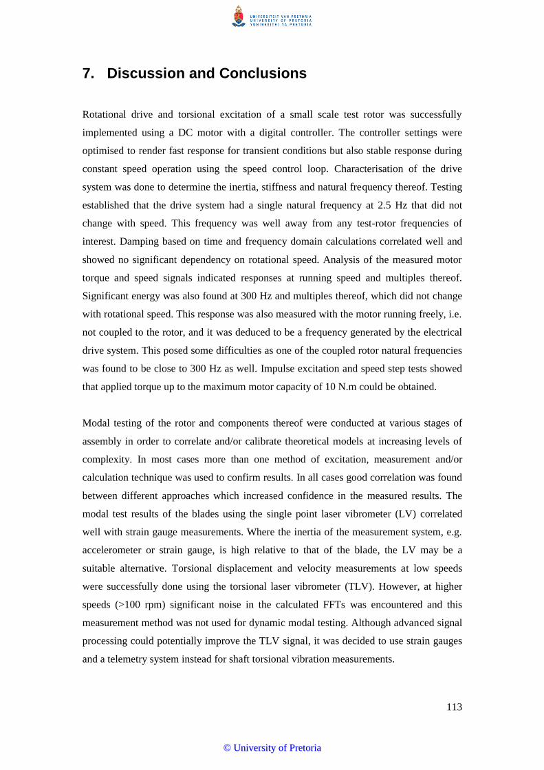
113

7. Discussion and Conclusions

Rotational drive and torsional excitation of a small scale test rotor was successfully

implemented using a DC motor with a digital controller. The controller settings were

optimised to render fast response for transient conditions but also stable response during

constant speed operation using the speed control loop. Characterisation of the drive

system was done to determine the inertia, stiffness and natural frequency thereof. Testing

established that the drive system had a single natural frequency at 2.5 Hz that did not

change with speed. This frequency was well away from any test-rotor frequencies of

interest. Damping based on time and frequency domain calculations correlated well and

showed no significant dependency on rotational speed. Analysis of the measured motor

torque and speed signals indicated responses at running speed and multiples thereof.

Significant energy was also found at 300 Hz and multiples thereof, which did not change

with rotational speed. This response was also measured with the motor running freely, i.e.

not coupled to the rotor, and it was deduced to be a frequency generated by the electrical

drive system. This posed some difficulties as one of the coupled rotor natural frequencies

was found to be close to 300 Hz as well. Impulse excitation and speed step tests showed

that applied torque up to the maximum motor capacity of 10 N.m could be obtained.

Modal testing of the rotor and components thereof were conducted at various stages of

assembly in order to correlate and/or calibrate theoretical models at increasing levels of

complexity. In most cases more than one method of excitation, measurement and/or

calculation technique was used to confirm results. In all cases good correlation was found

between different approaches which increased confidence in the measured results. The

modal test results of the blades using the single point laser vibrometer (LV) correlated

well with strain gauge measurements. Where the inertia of the measurement system, e.g.

accelerometer or strain gauge, is high relative to that of the blade, the LV may be a

suitable alternative. Torsional displacement and velocity measurements at low speeds

were successfully done using the torsional laser vibrometer (TLV). However, at higher

speeds (>100 rpm) significant noise in the calculated FFTs was encountered and this

measurement method was not used for dynamic modal testing. Although advanced signal

processing could potentially improve the TLV signal, it was decided to use strain gauges

and a telemetry system instead for shaft torsional vibration measurements.


114

Five torsional modes for the uncoupled rotor were measured at frequencies ranging from

~10 Hz to 725 Hz for static conditions. Once coupled to the motor armature some

frequencies increased, some decreased and one was un-affected. The uncoupled mode at

725 Hz was not measured for the coupled case and it is suspected to have increased to >1

kHz which is the limit of the telemetry system. A new mode at ~200 Hz was identified for

the coupled configuration. When the motor field and armature current is activated for the

dynamic tests the frequencies for 2 modes (F3a and F3b) decreased by 10 and 16 Hz whilst

the other two modes were unaffected. Eigen vector plots of the affected modes showed a

high level of participation of the armature in these modes and it is suspected that

electromagnetic forces and/or winding movement in the dynamic condition changes the

stiffness of the armature. The lowest frequency static mode at ~10 Hz was not detected in

any of the dynamic cases. From these findings it is clear that stationary modal testing,

especially with a coupled electrical machine such as a motor or generator, may not be

representative of the dynamic conditions. Modes with high levels of participation of

blades are affected significantly by the blade stagger angle. For the speed range tested no

significant relation between torsional frequencies and rotational speed was detected,

except for one mode with blades at 45° which showed a slight decrease with speed for

both random excitation and impulse tests.

Damping calculated by the half power method for static conditions showed a clear

reduction in most modes as the blade stagger angle was increased from 0 to 90°. One

mode with the lowest level of blade participation showed only a minimal reduction.

Although the general trend of damping measured for the dynamic cases is also that of a

reducing value with blade stagger angle, the relationship is not that clear. Due to poorly

defined FRF peaks for the dynamic cases, errors in the calculations are likely and an

alternative method should be applied. Blade stagger angle was demonstrated to affect

both the frequency and damping of torsional modes and should thus be considered in any

analysis involving flexible blades. Rotational speed did not have a significant effect on

damping. At most the damping of some modes reduce slightly with increasing speed.

Only torsional mode F3a, involving significant participation of disk #1 (disk with blades),

was detected in the blade responses during forced excitation tests. In addition, four rigid

shaft modes (two each of the 1st and 2nd blade bending modes) were seen in the blade

response. Two torsional modes, not involving a high degree of blade or blade carrier disk

participation, were not detected in the blade response. Only the rigid shaft modes where


115

all blades are in phase were detected in the torsional vibration response. It is thus clear

that blade frequency response cannot be inferred from shaft torsional response but has to

be measured or calculated specifically. Vice versa, not all torsional frequencies can be

detected by only considering blade response.

3D modelling of subsets of components and comparison to experimental data is useful to

ensure better accuracy of the assembled structure and to identify potential sources of

inaccuracy. A high degree of geometric detail was included in the parametric 3D model,

some of which may be simplified to reduce the model size. It was considered necessary to

include this level of detail so as to take full advantage of the capabilities of 3D modelling.

The two shrunk-on disks were modelled to be integral to the shaft and this proved to

result in acceptable accuracy in this case. In other cases where the interference fit may be

lower and/or the geometry unfavorable, it may be necessary to consider additional disk-

to-shaft flexibility. Assuming the effective coupling contact area to be up to the point of

the coupling grub screw or key proved to be an acceptable approach. It resulted in longer

shaft sections and slightly lower frequencies for some modes. For shrunk-on couplings

the same approach as with shrunk-on disks should be considered.

Accurate modelling of the motor armature was not attempted in this work. The armature

geometry was modelled as per measured dimensions and the stiffness thereof optimised

by calibration to measured static and 250 rpm frequencies for the 0° blade case.

Application of this stiffness in all other cases resulted in acceptable accuracy. Density of

the armature winding section was calibrated so that the modelled inertia was equal to that

measured using the torsional pendulum approach. Modelling of electrical machines for

the purpose of torsional and lateral vibration simulation remains a challenge that requires

further research. Currently model updating with measured data remains the preferred and

most accurate approach. Modal analysis by 3D FEA allows for the visualization of eigen-

modes and can also identify modes that are not measured. Good correlation of predicted

torsional frequencies was obtained with measured results with errors generally below 1%

except for two modes (F2 and F3a) in the case of the static uncoupled rotor with blades at

45° which is at 1.6 and 1% respectively.


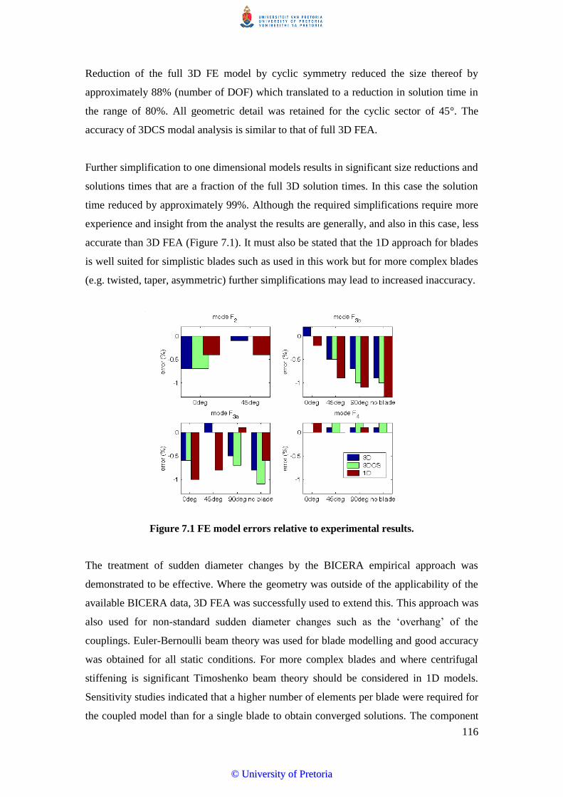
116

Reduction of the full 3D FE model by cyclic symmetry reduced the size thereof by

approximately 88% (number of DOF) which translated to a reduction in solution time in

the range of 80%. All geometric detail was retained for the cyclic sector of 45°. The

accuracy of 3DCS modal analysis is similar to that of full 3D FEA.

Further simplification to one dimensional models results in significant size reductions and

solutions times that are a fraction of the full 3D solution times. In this case the solution

time reduced by approximately 99%. Although the required simplifications require more

experience and insight from the analyst the results are generally, and also in this case, less

accurate than 3D FEA (Figure 7.1). It must also be stated that the 1D approach for blades

is well suited for simplistic blades such as used in this work but for more complex blades

(e.g. twisted, taper, asymmetric) further simplifications may lead to increased inaccuracy.

Figure 7.1 FE model errors relative to experimental results.

The treatment of sudden diameter changes by the BICERA empirical approach was

demonstrated to be effective. Where the geometry was outside of the applicability of the

available BICERA data, 3D FEA was successfully used to extend this. This approach was

also used for non-standard sudden diameter changes such as the ‘overhang’ of the

couplings. Euler-Bernoulli beam theory was used for blade modelling and good accuracy

was obtained for all static conditions. For more complex blades and where centrifugal

stiffening is significant Timoshenko beam theory should be considered in 1D models.

Sensitivity studies indicated that a higher number of elements per blade were required for

the coupled model than for a single blade to obtain converged solutions. The component


117

mode synthesis technique used to include the blade participation effects in torsional

vibration modes was successfully implemented and good accuracies were obtained.

It is concluded that all three FE techniques applied here to model torsional vibration

response are useful and have their place. Fast solution times of 1D models allows for

sensitivity studies in the design and fault finding environments to be conducted with

relative ease, although the accuracy is likely to be somewhat less than 3D FE approaches.

Simplifications required for the 1D approach can be extensive and may require input from

more detailed 3D analysis of some aspects.

If detailed blade vibration response is required the 3D approaches would be more

suitable. Full 3D analysis does not require significant simplification, if at all, and with

currently available modelling software can be developed in a short time. Although modal

analysis of these models require significantly more solution time than 1D models, the

actual time for a single point solution is still acceptable. However, for full transient

analysis solution times for 3D models may be limiting.

3D cyclic symmetric analysis which still captures all the geometric detail of the 3D

models is a good approach to apply when a high level of accuracy and faster solution

times are required. Depending on the design the specification of the 3D sector may be

complicated and require some form of simplification if it does not capture all the

geometry exactly in a single sector. Another disadvantage, with respect to full 3D FE, is

that the effect of mistuned blades cannot be simulated. In all modelling cases, where a

high level of accuracy is required, the level of simplification generally used is likely to

result in unacceptably high errors. As such model calibration or model updating with

measured results should be applied.

Further work in the field of torsional vibration measurement and finite element simulation

should include:

Methodologies to simulate motors/generators.

Methodology to simplify complex blades to equivalent mass and stiffness values.

Model updating methodology to increase model accuracy.

Investigate the use of torsional laser vibrometers and advanced signal processing

to improve measurement accuracy at speed.


118

Effect of blade mistuning on torsional vibration behaviour.

Multi-stage cyclic symmetric FE analysis.

Effect of temperature and temperature distribution

Non-linear effects due to blade vibration damping mechanisms such as tie-wires,

integral shrouds and snubbers.

Disk participation in the case of slender and flexible disks

Effect of blade mode shapes and torsional stiffening

Investigate the use of time domain analysis of filtered modal signals for the

estimation of modal damping


119

BIBLIOGRAPHY

Al-Bedoor, B. (1999). Dynamic model of coupled shaft torsional and blade bending

deformations in rotors. Computer Methods in Applied Mechanics and

Engineering, 5(169), 177–190.

Al-Bedoor, B., & Al-Qaisia, A. (2005). Stability analysis of rotating blade bending

vibration due to torsional excitation. Journal of Sound and Vibration, 282, 1065–

1083. doi:10.1016/j.jsv.2004.03.038

Al-Nassr, Y., & Al-Bedoor, B. (2003). On the Vibration of a Rotating Blade on a

Torsioally Flexible Shaft. Journal of Sound and Vibration, 259(5), 1237–1242.

doi:10.1006/jsvi.2002.5287

Anegawa, N., Fujiwara, H., & Matsushita, O. (2011). Vibration Diagnosis Featuring

Blade-Shaft Coupling Effect of Turbine Rotor Models. Journal of Engineering

for Gas Turbines and Power, 133(February), 1–8. doi:10.1115/1.4001980

Bahrman, M. P., Larsen, E., Piwko, R., Parel, H., Hauth, R., & Breur, G. (1980).

HVDC - Turbine-generator Torsional Intercations A New Design Consideration.

In International Conference on Large High Voltage Electric Systems (pp. 1–9).

Bai, B., Zhang, L., Guo, T., & Liu, C. (2012). Analysis of Dynamic Characteristics of

the Main Shaft System in a Hydro-turbine Based on ANSYS. Procedia

Engineering, 31(2011), 654–658. doi:10.1016/j.proeng.2012.01.1081

Bernasconi, O. (1986). Solution for torsional vibrations of stepped shafs using

singularity functions. International Journal of Mechanical Sciences, 28(1), 31–

39.

Bhartiya, Y., & Sinha, A. (2012). Reduced Order Model of a Multistage Bladed Rotor

With Geometric Mistuning via Modal Analyses of Finite Element Sectors.

Journal of Turbomachinery, 134(July), 1–8. doi:10.1115/1.4003224


120

Bladh, R., Pierre, C., Castanier, M. P., & Kruse, M. J. (2002). Dynamic Response

Predictions for a Mistuned Industrial Turbomachinery Rotor Using Reduced-

Order Modeling. Journal of Engineering for Gas Turbines and Power,

124(April), 311–324. doi:10.1115/1.1447236

Bovsunovskii, A., Chernousenko, O., & Shtefan, E. (2010). Fatigue Damage and

failure of steam turbine rotors by torsional vibration. Strength of Materials,

42(1), 108–113.

Brower, A., Bowler, C., & Edmonds, J. (1988). Long Term Torsional Vibration

Monitoring on Large Steam Turbine Generators. In CIGRE International

Conference on Large High Voltage Electric Systems (pp. 1–7).

Chandrupatla, T., & Belengundu, A. (2003). Introduction to Finite Elements in

Engineering (3rd ed.). Prentice Hall.

Chatelet, E., D’Ambrosio, F., & Jacquet-Richardet, G. (2005). Toward global

modelling approaches for dynamic analyses of rotating assemblies of

turbomachines. Journal of Sound and Vibration, 282, 163–178.

doi:10.1016/j.jsv.2004.02.035

Chen, Y. (2004). An Investigation of excitation method for torsional testing of a large

scale steam turbine generator. Journal of Vibration and Acoustics, 126, 163–167.

Chiu, Y., & Chen, D. (2011). The coupled vibration in a rotating multi disk rotor

system. International Journal of Mechanical Sciences, 53(1), 1–10.

doi:10.1016/j.ijmecsci.2010.10.001

Chivens, D., & Nelson, H. (1975). The Natural Frequencies and Critical Speeds of a

Rotating , Flexible - Shaft-Disk System. Journal Of Engineering For Industry,

(August), 881–886.

Chyn, C., Wu, R., & Tsao, T. (1996). Torsional fatigue of turbine-generator shafts

owing to network faults. IEE Proc.-Gener. Transm. Distrib, 143(5), 479–486.


121

Cook, R., Malkus, D., Plesha, M., & Witt, R. (2002). Concepts and Applications of

Finite Element Analysis (4th ed.). United States: John Wiley & Sons.

Crawley, E. F., Ducharme, E. H., & Mokodam, D. R. (1986). Analytical and

experimental investigation of the coupled disk shaft whirl of a cantilevered

turbofan. Journal of Engineering for Gas Turbines and Power, 108(October),

567–576.

Crawley, E. F., & Mokadam, D. R. (1984). Stagger Angle Dependence of Inertial and

Elastic Coupling in Bladed Disks, 106(April), 181–188.

Doughty, S. (1985). Transfer Matrix Eigensolutions for Damped Torsional Systems.

Journal of Vibration, Acoustics, Stress and Reliability Design, 107, 128.

Drew, S., & Stone, B. (1997). Torsional (Rotational) vibration: Excitation of small

rotating machines. Journal of Sound and Vibration, 201(4), 437–463.

Dunlop, R., Horowitz, S., Joyce, J., & Lambrecht, D. (1980). Torsional Oscillations

and Fatigue of Steam Turbine-Generator Shafts Caused by System Disturbances

and Switching Events. In CIGRE International Conference on Large High

Voltage Electric Systems (Vol. 33, pp. 1–19).

EPRI. (2005a). Steam Turbine-Generator Torsional Vibration Interaction with the

Electrical Network. EPRI.

EPRI. (2005b). Technology Development for Shaft Crack Detection in Rotating

Equipment in NPP Using Torsional Vibration. Manager (pp. 2–13).

Genta, G. (2008). Present and future trends in rotordynamic analysis.

Hammons, T. J. (1982). Accumulative Fatigue Life Expenditure of Turbine Generator

Shafts Following Worst Case System Disturbances. IEEE Transactions on

Power Apparatus and Systems, PAS-101(7), 2364–2374.

Hammons, T. J., & Mcgill, J. F. (1993). Comparison of turbine-generator shaft

torsional response predicted by frequency domain and time domain methods.

IEEE Transactions on Energy Conversion, 8(3), 559–565.


122

Hoffmann, K. (1989). An Introduction to Measurements using Strain Gages. Alsbach,

Germany: Hottinger Baldwin Messtechnik GmbH.

Huang, D. G. (2007). Characteristics of torsional vibrations of a shaft with unbalance.

Journal of Sound and Vibration, 308, 692–698. doi:10.1016/j.jsv.2007.04.005

Huang, S., & Ho, K. (1996). Coupled Shaft-Torsion and Blade-Bending Vibrations of

a Rotating Shaft-Disk-Blade Unit. Journal of Engineering for Gas Turbines and

Power, 118, 100–106.

IEEE. (1992). Reader’s Guide to Subsynchronous Resonance. IEEE Tansactions on

Power Systems, 7(1), 150–157.

Imregun, M., & Visser, W. J. (1991). Multistage beam modelling of turbomachinery

blades. Finite Elements in Analysis and Design, 10, 41–57.

Jacquet-Richardet, G., & Dal-Ferro, C. (1996). Reduction Method for Finite Element

Dynamic Analysis of Submerged Turbomachinery Wheels. Computers, 61(6),

1025–1036.

Jacquet-Richardet, G., Ferraris, G., & Rieutord, P. (1996). Frequencies and modes of

rotating flexible bladed disc-shaft assemblies: A global cyclic symmetric

approach. Journal of Sound and Vibration, 191(5), 901–915.

Joshi, B., & Dange, Y. (1976). Critical Speeds of a Flexible Rotor with Combined

Distributed Parameter and Lumped Mass Technique. Journal of Sound and

Vibration, 45(3), 441–459.

Khader, N., & Loewy, R. G. (1990). Shaft flexibility effects on the forced response of

a bladed disk assembly. Journal of Sound and Vibration, 139(3), 469–485.

Kim, Y., Yang, B., & Kim, C. (2006). Noise Source Identification of Small Fan-

BLDC Motor System for Refrigerators. International Journal of Rotating

Machinery, 2006, 1–7. doi:10.1155/IJRM/2006/63214


123

Kirkhope, J., & Wilson, G. J. (1976). A FINITE ELEMENT ANALYSIS FOR THE

VIBRATION MODES OF A BLADED DISC. Journal of Sound and Vibration,

49, 469–482.

Lambrecht, D., & Kulig, T. (1982). Torsional performance of turbine shafts especially

under resonant conditions. IEEE Tansactions on Power Apparatus and Systems,

PAS-101(10), 3689–3702.

Laxalde, D., & Pierre, C. (2011). Modelling and analysis of multi-stage systems of

mistuned bladed disks. Computers and Structures, 89(3-4), 316–324.

doi:10.1016/j.compstruc.2010.10.020

Leong, J. H., & Zhu, Z. Q. (2011). A Novel Torsional Excitation Scheme for

Determining Mechanical Transfer Function and Natural Frequencies of

Circumferential Vibration in PM Brushless Machine Drives, 47(10), 4195–4198.

Lund, J., & Wang, Z. (1986). Application of the Riccati Method to Rotor Dynamic

Analysis of Long Shafts on a Flexible Foundation. Journal of Vibration,

Acoustics, Stress and Reliability Design, 108(April), 177–181.

Mbaye, M., Soize, C., & Ousty, J. (2010). A Reduced-Order Model of detuned cyclic

dynamical systems with geometric modifications using a basis of cyclic modes.

Journal of Engineering for Gas Turbines and Power, 132(November), 1–9.

doi:10.1115/1.4000805

Meirovitch, L. (2001). Fundamentals of Vibrations. Singapore: McGraw-Hill.

Murphy, B., & Vance, J. M. (1983). An Improved Method for Calculating Critical

Speeds and Rotordynamic Stability of Turbomachinery. Journal Of Engineering

For Power, 105(July), 591–595.

Nagaraj, V., & Shanthakumar, P. (1975). Rotor blade vibrations by the Galerkin finite

element method. Journal of Sound and Vibration, 43(3), 575–577.

Nelson, H. (1998). Rotordynamic Modeling and Analysis Procedures: A Review.

Japan Society of Mechanical Engineers International Journal, 41(C), 1–12.


124

Okabe, A., Kudo, T., Shiohata, K., Matsushita, O., Fujiwara, H., Yoda, H., & Sakurai,

S. (2012). Reduced Modeling for Turbine Rotor-Blade Coupled Bending

Vibration Analysis. Journal of Engineering for Gas Turbines and Power,

134(February), 1–8. doi:10.1115/1.4004145

Okabe, A., Yoda, H., Matsushita, O., Kudo, T., Sakuri, S., & Shiohata, K. (2009).

Rotor Blade Coupled Vibration Analysis by measuring Modal Parameters of

Actual Rotor. In ASME Turbo Expo 2009:Power for land, sea and air (pp. 803–

812).

Omprakash, V. (1988). Analysis of bladed disks - A review. The Shock and Vibration

Digest, 11(20), 14–21.

Omprakash, V., & Ramamurti, V. (1988). Natural frequencies of bladed disks by a

combined cyclic symmetric symmetry and Raleigh-Ritz method. Journal of

Sound and Vibration, 125(2), 357–366.

Petrov, E. P. (2004). A Method for Use of Cyclic Symmetry Properties in Analysis of

Nonlinear Multiharmonic Vibrations of Bladed Discs. Journal of

Turbomachinery, 126(January), 175–183. doi:10.1115/1.1644558

Ricci, R., Pennacchi, P., Pesatori, E., & Turozzi, G. (2010). Modeling and Model

Updating of Torsional Behaviour of an Industrial Steam Turbo Generator.

Journal of Engineering for Gas Turbines and Power, 132(July), 1–7.

doi:10.1115/1.4000287

Roark, R. J., & Young, W. C. (1975). Formulas for Stress and Strain (5th ed.). United

States: McGraw-Hill.

Rouch, K. E., Mcmains, T. H., Stephenson, R. W., & Emerick, M. (1991). Modeling

of complex rotor systems by combining rotor and substructure models. Finite

Elements in Analysis and Design, 10, 89–100.

Santos, I. F., Saracho, C. M., Smith, J. T., & Eiland, J. (2004). Contribution to

experimental validation of linear and non-linear dynamic models for representing


125

rotor – blade parametric coupled vibrations, 271, 883–904. doi:10.1016/S0022-

460X(03)00758-2

Stephenson, R., Rouch, K., & Arora, R. (1989). Modelling of rotors with

axisymmetric solid harmonic elements. Journal of Sound and Vibration, 131(3),

431–443.

Sternchuss, A., Balnes, E., Jean, P., & Lombard, J. (2009). Reduction of Multistage

Disk Models: Application to an Industrial Rotor. Journal of Engineering for Gas

Turbines and Power, 131(January), 1–14. doi:10.1115/1.2967478

Szolc, T. (2000). On the Discrete-Continuous Modeling of Rotor Systems the

Analysis of Coupled Lateral Torsional Vibrations. International Journal of

Rotating Machinery, 6(2), 135–149.

Thomas, D. L. (1979). Dynamics of rotationally periodic structures. International

Journal for Numerical Methods in Engineering, 14(July), 81–102.

Tian, Y., Qi, X., & Hu, J. (2012). Comparison between two ANSYS finite element

modeling methods of multistage centrifugal pump rotor. Applied Mechanics and

Materials, 105-407, 2295–2298.

Tsai, J., Lin, C., & Tsao, T. (2004). Assessment of Long-Term Life Expenditure for

Steam Turbine Shafts Due to Noncharacteristic Subharmonic Currents in

Asynchronous Links. IEEE Transactions on Power Systems, 19(1), 507–516.

Tsai, W. (2001). Improvement in the corrosive fatigue damage to the low-pressure

steam turbine blades due to unbalanced currents, 59, 139–148.

Tsai, W.-C., Tsao, T., & Chyn, C. (1997). A nonlinear model for the analysis of the

turbine-generator vibrations including the design of a flywheel damper.

Electrical Power & Energy Systems, 19(7), 469–479.

Tse, F. S., Morse, I. E., & Hinkle, R. (1978). Mechanical Vibrations, Theory and

Applications. United States: Prentice-Hall.


126

Turhan, O., & Bulut, G. (2006). Linearly coupled shaft-torsional and blade-bending

vibrations in multi-stage rotor-blade systems. Journal of Sound and Vibration,

296, 292–318. doi:10.1016/j.jsv.2006.03.010

Vance, J. M., Murphy, B., & Tripp, H. (1987). Critical Speeds of Turbomachinery:

Computer Predictions vs . Experimental Measurements — Part I: The Rotor

Mass — Elastic Model. Journal of Vibration, Acoustics, Stress and Reliability

Design, 109(January), 1–7.

Walker, D. N. (2004). Torsional Vibration of Turbomachinery. New York (USA):

McGraw-Hill.

Wu, F., & Flowers, G. (1992). A transfer matrix technique for evaluating the natural

frequencies and critical speeds of a rotor with multiple flexible disks. Journal of

Vibration and Acoustics, 114(April), 241–248.

Xie, D., Huang, J., Wan, J.-F., & Yuan, Y. (2003). Analysis on Problems of

Removing the Odd Point in Rotors Torsional Vibration Characteristics

Calculation Using Riccati Method. In Second International Conference on

Machine Learning and Cybernetics (pp. 2185–2188).

Xie, D., Li, W., Yang, L., Qian, Y., Zhao, X., & Gao, Z. (2010). A General

Calculating Method of Rotor ’ s Torsional Stiffness Based on Stiffness Influence

Coefficient. In Power and Energy Engineering Conference (APPEEC) (Vol. 2,

pp. 698–704). doi:10.4236/eng.2010.29090

Yang, C., & Huang, S. (2007). Coupling Vibrations in Rotating Shaft-Disk-Blades

System. Journal of Vibration and Acoustics, 129(2), 48–57.

doi:10.1115/1.2221328


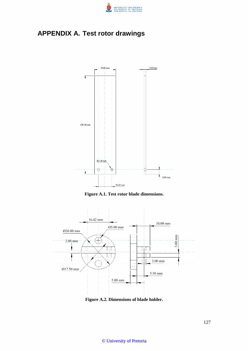
127

APPENDIX A. Test rotor drawings

Figure A.1. Test rotor blade dimensions.

Figure A.2. Dimensions of blade holder.


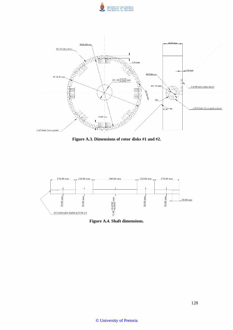
128

Figure A.3. Dimensions of rotor disks #1 and #2.

Figure A.4. Shaft dimensions.


129

Figure A.5. Motor coupling dimensions.

Figure A.6. Rotor shaft coupling dimensions


130

Figure A.7. DC motor armature dimensions.


131

APPENDIX B. Armature lateral shaft modes

Modal tests were conducted using the modal hammer and the Polytec PFV100 laser

vibrometer to determine the lateral vibration frequencies of the armature. The armature

was placed on two supports for the bearings. Impacts in all tests were done on the

coupling flange and measurements taken as per Figure B.1.

Figure B.1. Measurement positions for lateral modes.

In all cases impacts and measurements were done in line with the coupling grub screw as

well as 90° from this position. A set of tests were done impacting and measuring in the

vertical direction as well as a set where impacts and measurements were done in the

horisontal direction. Figure B.2 shows the setup for vertical tests.

Figure B.2 Setup for vertical modal tests to determine lateral modes.


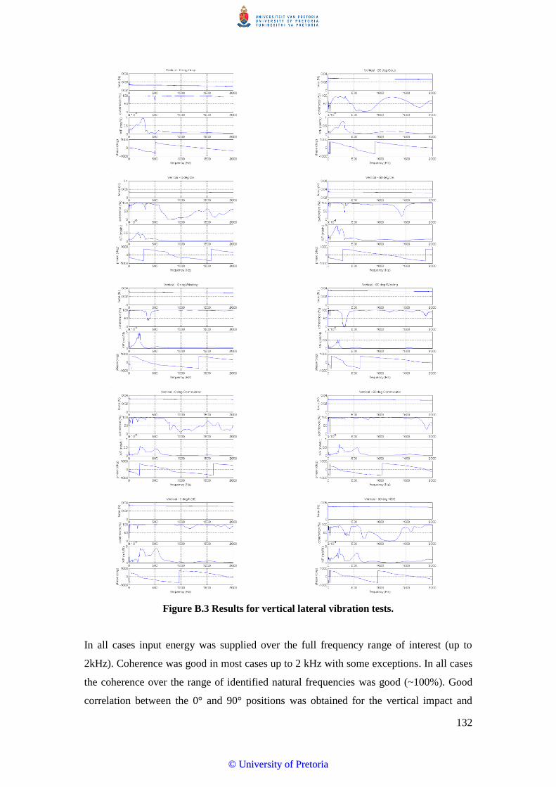
132

Figure B.3 Results for vertical lateral vibration tests.

In all cases input energy was supplied over the full frequency range of interest (up to

2kHz). Coherence was good in most cases up to 2 kHz with some exceptions. In all cases

the coherence over the range of identified natural frequencies was good (~100%). Good

correlation between the 0° and 90° positions was obtained for the vertical impact and


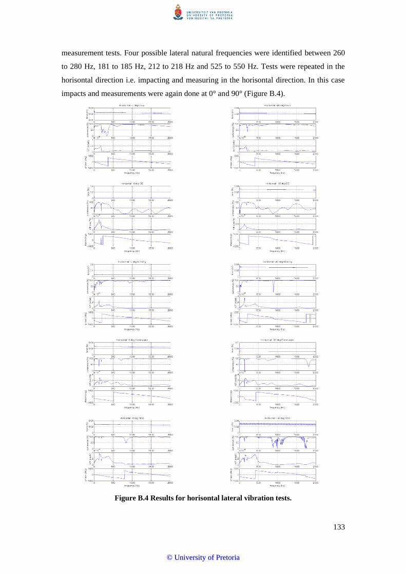
133

measurement tests. Four possible lateral natural frequencies were identified between 260

to 280 Hz, 181 to 185 Hz, 212 to 218 Hz and 525 to 550 Hz. Tests were repeated in the

horisontal direction i.e. impacting and measuring in the horisontal direction. In this case

impacts and measurements were again done at 0° and 90° (Figure B.4).

Figure B.4 Results for horisontal lateral vibration tests.


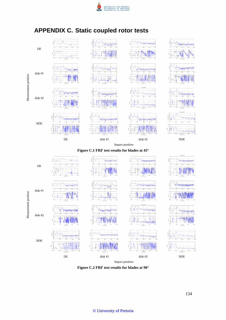
134

APPENDIX C. Static coupled rotor tests M

easu

rem

ent

po

siti

on

DE

disk #1

disk #2

NDE


Impact position

Figure C.1 FRF test results for blades at 45°

Mea

sure

men

t po

siti

on

DE

disk #1

disk #2

NDE


Impact position

Figure C.2 FRF test results for blades at 90°


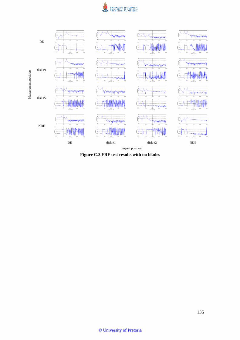
135

Mea

sure

men

t po

siti

on

DE

disk #1

disk #2

NDE


Impact position

Figure C.3 FRF test results with no blades


136

APPENDIX D. Rigid shaft modes

The lowest seven rigid shaft modes, also referred to as repeated modes, are shown in

Figure D.1 below.

144.93 Hz 144.95 Hz 145.06 Hz 145.22 Hz

145.31 Hz 145.32 Hz 145.33 Hz

Figure D.1. Rigid shaft modes.


137

APPENDIX E. Transient dynamic analysis

Speed step tests were done where a step function of 1V was applied to a nominally

stationary rotor and the blade stress response measured. The rotor accelerates to ~300 rpm

for the 1V control signal.

Figure E.1. Speed step test data.

Time sequences from the blade stress response signal was extracted from the data for zero

rpm, the pulse as well as constant speed running at 280 rpm. FFTs of these sequences

were done to calculate the frequency content. At rest and in the STOP mode the strain

gauge noise signal contains frequencies at 144 and 896 Hz, the 1st and 2nd blade modes. It

also contains ~152 and ~337 Hz, the F2 and F3a modes measured during static modal tests.

The blade stress response due to the torque impulse loading shows frequency content at

~144 Hz and 896 Hz; the 1st and 2nd blade modes. The most energy appears to be in the 1st

torsional mode at ~152 Hz. There is also a strong component of the 300 Hz control signal.

The stress response signal at a constant 300 rpm have components at the blade 1st and 2nd

modes i.e. 144 and 895Hz as well as the 300Hz control system frequency. A ~5 Hz peak

at the running speed was also noted.

Blade stress peaks at ~9MPa for peak torques of ~8N.m.


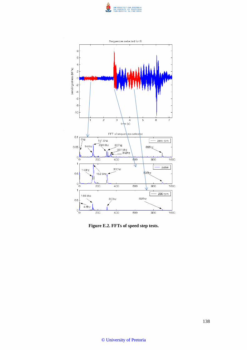
138

Figure E.2. FFTs of speed step tests.


139

Figure E.3. Typical torque pulse for a speed step test.

The torque signal in the STOP mode has low amplitude components at 300Hz and

multiples thereof. During the pulse the 300 Hz signal is the most dominant, except for the

low frequency component. In the constant 300 rpm state multiples of line frequency and

300 Hz (dominant) can be seen.

Figure E.4. FFT of torque signal sequences.

Using 2nd order Butterworth bandstop filters the measured blade time stress response is

filtered to remove frequencies at 300, 144, 896 and 152 Hz as well as the floor noise

(Figure E.5). The remaining signal clearly shows the stress response due to the torque

pulse as well as the cyclic stress due to self-weight.


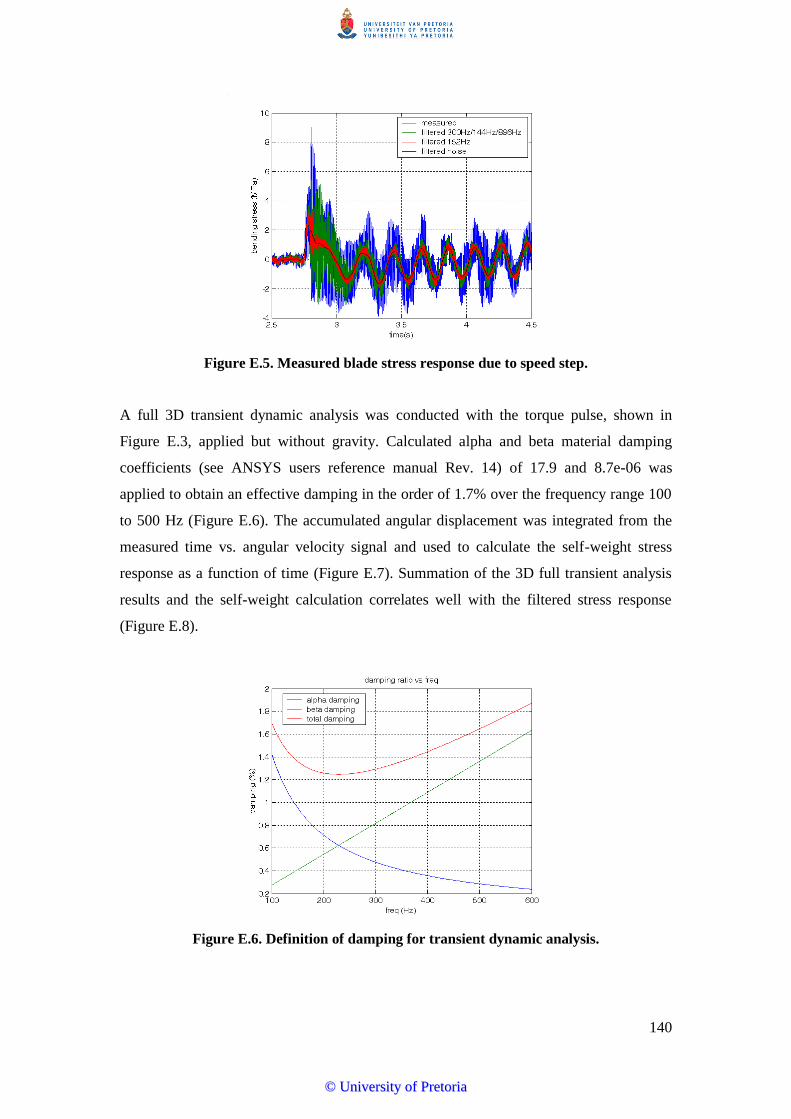
140

Figure E.5. Measured blade stress response due to speed step.

A full 3D transient dynamic analysis was conducted with the torque pulse, shown in

Figure E.3, applied but without gravity. Calculated alpha and beta material damping

coefficients (see ANSYS users reference manual Rev. 14) of 17.9 and 8.7e-06 was

applied to obtain an effective damping in the order of 1.7% over the frequency range 100

to 500 Hz (Figure E.6). The accumulated angular displacement was integrated from the

measured time vs. angular velocity signal and used to calculate the self-weight stress

response as a function of time (Figure E.7). Summation of the 3D full transient analysis

results and the self-weight calculation correlates well with the filtered stress response

(Figure E.8).

Figure E.6. Definition of damping for transient dynamic analysis.


141

Figure E.7. Blade stress response due to self-weight.

Figure E.8. Calculated blade stress response.

High measured dynamic content at the 1st and 2nd blade bending modes are suspected to

be enhanced by aerodynamic effects which were unaccounted for in the transient analysis.


Documents

A COMPARATIVE STUDY OF FINITE ELEMENT METHODOLOGIES …