Embed Size (px)
Citation preview

A Comparative Study of Secondary Indexing Techniques inLSM-based NoSQL Databases
Mohiuddin Abdul Qader, Shiwen Cheng, Vagelis Hristidis
{mabdu002,schen064,vagelis}@cs.ucr.edu
Department of Computer Science & Engineering, University of California Riverside
ABSTRACTNoSQL databases are increasingly used in big data applications,
because they achieve fast write throughput and fast lookups on the
primary key. Many of these applications also require queries on
non-primary attributes. For that reason, several NoSQL databases
have added support for secondary indexes. However, these works
are fragmented, as each system generally supports one type of
secondary index, and may be using different names or no name
at all to refer to such indexes. As there is no single system that
supports all types of secondary indexes, no experimental head-to-
head comparison or performance analysis of the various secondary
indexing techniques in terms of throughput and space exists. In
this paper, we present a taxonomy of NoSQL secondary indexes,
broadly split into two classes: Embedded Indexes (i.e. lightweightfilters embedded inside the primary table) and Stand-Alone Indexes(i.e. separate data structures). To ensure the fairness of our compara-
tive study, we built a system, LevelDB++, on top of Google’s popular
open-source LevelDB key-value store. There, we implemented two
Embedded Indexes and three state-of-the-art Stand-Alone indexes,
which cover most of the popular NoSQL databases. Our compre-
hensive experimental study and theoretical evaluation show that
none of these indexing techniques dominate the others: the embed-
ded indexes offer superior write throughput and are more space
efficient, whereas the stand-alone secondary indexes achieve faster
query response times. Thus, the optimal choice of secondary in-
dex depends on the application workload. This paper provides an
empirical guideline for choosing secondary indexes.
ACM Reference Format:Mohiuddin Abdul Qader, Shiwen Cheng, Vagelis Hristidis. 2018. A Com-
parative Study of Secondary Indexing Techniques in LSM-based NoSQL
Databases. In SIGMOD’18: 2018 International Conference on Managementof Data, June 10–15, 2018, Houston, TX, USA. ACM, New York, NY, USA,
16 pages. https://doi.org/10.1145/3183713.3196900
1 INTRODUCTIONIn the age of big data, more and more services are required to ingest
high volume, velocity and variety data, such as social networking
data, smartphone apps usage data and click through data. NoSQL
Permission to make digital or hard copies of all or part of this work for personal or
classroom use is granted without fee provided that copies are not made or distributed
for profit or commercial advantage and that copies bear this notice and the full citation
on the first page. Copyrights for components of this work owned by others than the
author(s) must be honored. Abstracting with credit is permitted. To copy otherwise, or
republish, to post on servers or to redistribute to lists, requires prior specific permission
and/or a fee. Request permissions from [email protected].
SIGMOD’18, June 10–15, 2018, Houston, TX, USA© 2018 Copyright held by the owner/author(s). Publication rights licensed to Associa-
tion for Computing Machinery.
ACM ISBN 978-1-4503-4703-7/18/06. . . $15.00
https://doi.org/10.1145/3183713.3196900
databases were developed as a more scalable and flexible alterna-
tive to relational databases. NoSQL databases, such as HBase [13],
Cassandra [31], Voldemort [12], MongoDB [26], AsterixDB [2] and
LevelDB [23] to name a few, have attracted huge attention from in-
dustry and research communities, and are widely used in products.
Through the use of Log-Structured Merge-Tree (LSM) [34], NoSQL
systems are particularly good at supporting two capabilities: (a) fast
write throughput, and (b) fast lookups on the primary key of a data
entry (See Appendix A.1 for details on LSM storage framework).
However, many applications also require queries on non-key at-
tributes which is a functionality commonly supported in RDBMSs.
For instance, if a tweet has attributes such as tweet id, user id and
text, then it would be useful to be able to return all (or the most
recent) tweets of a user. However, supporting secondary indexes
in NoSQL databases is challenging, because secondary indexing
structures must be maintained during writes, while also managing
the consistency between secondary indexes and data tables. This
significantly slows down writes, and thus hurts the system’s capa-
bility to handle high write throughput which is one of the most
important reasons why NoSQL databases are used.
Table 1 shows the operations that we want to support. The first
three operations (GET, PUT and DEL) are already supported by ex-
istingNoSQL stores like LevelDB. Note that the secondary attributes
and their values are stored inside the value of an entry, which may
be in JSON format: v = {A1 : val (A1) , · · · ,Al : val (Al )}, whereval(Ai ) is the value for the secondary attribute Ai . For example,
the key of a tweet entry could be k = tweet id , A1 = user id and
A2 = body text . Key k should not be confused with limit K (top-K ),which means K most recent records in terms of insertion time in
the database.
Table 1: Set of operations in a NoSQL database.Operation DescriptionGET (k ) Retrieve value identified by primary key k .PUT (k , v ) Write a new entry ⟨k, v ⟩ (or overwrite if k already
exists), where k is the primary key.
DEL (k ) Delete the entry identified by primary key k if any.
LOOKUP (A, a, K ) Retrieve theK most recent entries withval (A) = a.RANGELOOKUP (A,a, b , K )
Retrieve the K most recent entries with a ≤val (A) ≤ b .
Stand-Alone Secondary Indexes. Current NoSQL systems have
adopted different strategies to support secondary indexes (e.g., on
the user id of a tweet). Most of them maintain a separate Stand-
Alone Index table. For instance, MongoDB [26] uses B+-tree for
secondary index, which follows the same way of maintaining sec-
ondary indexes as traditional RDBMSs. They perform in-place up-
dates (which we refer as “Eager” updates, and we refer to such
indexes as Eager Indexes) of the B+ tree secondary index, that is,
for each write in the data table the index (e.g., B+ tree) is updated.
In the case of some LSM-based NoSQL systems (e.g., BigTable [5]),

(a) Comparison between Eager and Lazy updates, and <secondary+primary> Composite keys in Stand-Alone Indexes
(b) Zone maps and bloom filters in Embedded Index
Figure 1: Comparison between various secondary indexes after operations in Example 1. We use the notation key → value.
which store a secondary index as an LSM table (column family),
an Eager update is technically not in-place, but a new posting list
is written that invalidates the older ones. In contrast to in-place
updates, other LSM-based systems (e.g., Cassandra [31]) perform
append-only updates on the LSM index table, which we refer as
“Lazy” updates, and Lazy Indexes.
Example 1. Consider the current state of a database right afterthe following sequence of operations PUT(t1, {u1, text1}),PUT(t2, {u1,text2}),PUT(t3, {u1, text3},· · · ), where ti is a tweet id, ui is a userid, and texti is the text of a tweet. Then, as shown in Figure 1(a),to execute PUT(t4, {u1, text4}) on an Eager Index, we must retrievethe list for u1, add t4 and save it back, whereas for a Lazy Index,we simply issue a PUT(u1, {t4}) on the user id index table withoutretrieving the existing posting list for u1. The old postings list of u1 ismerged with (u1, {t4}) later, during the periodic compaction phase.
A drawback of the lazy update strategy is that reads on index
tables become slower, because they have to merge the posting lists
at query time. Earlier versions of Cassandra handled this by first
accessing the index table to retrieve the existing posting list of u1,
then writing back a merged posting list to the index table. Then
the old posting list becomes obsolete. However, this Eager Index
degrades the write performance.
In addition to these Stand-Alone indexes which maintain posting
lists, several systems (e.g. AsterixDB [2], Spanner [7]) adopt a dif-
ferent approach to maintain the secondary indexes, which we refer
as Composite Index. Here, each entry in the secondary indexes is a
composite key consisting of (secondary key + primary key). The
secondary lookup is a prefix search on secondary key, which can be
implemented using regular range search on the index table. Here,
writes and compactions are faster than “Lazy,” but secondary at-
tribute lookup may be slower as it needs to perform a range scan on
the index table. We have implemented Eager, Lazy and Composite
Stand-Alone Indexes. All these indexes can naturally support both
lookup and range queries.
Embedded Secondary Indexes. We also built Embedded indexes,which differ in that there is no separate secondary index structure,
but secondary attribute information is stored inside the original
(primary) data blocks. We built two Embedded Indexes. The first is
based on bloom filters [4], which are a popular hashing technique
for set membership check (See Appendix A.3 for details on bloom
filters). Bloom filters are already being used for primary indexing in
many systems such as BigTable[5], LevelDB[23] and AsterxiDB[2].
But surprisingly, to our best knowledge, it has not been used for
secondary attribute lookup in any of the existing NoSQL system. A
drawback of bloom filter index is that it can only support lookup
queries.
In addition to bloom filters, we also implement another Em-
bedded Index, zone maps, which typically store the minimum and
maximum values of a column (attribute) in a table per disk block.
Zone maps are used in Oracle [27], Netezza [25], and AsterixDB [2].
Zone maps can be used for both lookup and range queries. How-
ever, in practice, zone maps are only useful when the incoming
data is time-correlated, otherwise most of the data blocks have to
be examined [2]. An attribute is called time-correlated if its value
for a record is highly correlated with the record’s insertion times-
tamp. For example, tweet-id is time-correlated because the tweet-id
value increases with time. Note that the higher the correlation the
stronger pruning we achieve in zone maps. No index’s or algo-
rithm’s correctness requires that an attribute is time-correlated.
Note that these Embedded Indexes do not create any specialized
index structure, but instead attach a memory-resident bloom fil-
ter signature and a zone map to each data block for each indexed
secondary attribute. As LSM files on disks (called SSTables, see Ap-
pendix A.2) are immutable, these filters do not need to be updated;
they are naturally computed when an SSTable is created. In ourexperiments, we consider both bloom filters and zone maps togetheras one index, which we refer as Embedded Index.Example 1 (cont’d) Figure 1 shows the differences between the fiveindexing strategies. As in LSM-style storage structures, data are or-ganized as levels, three levels shown in Figure 1, where the top rowis in-memory and the bottom two on disk. Lower levels are generallylarger and store older data. In some systems like LevelDB, lower levels

have more SSTables of the same size, and in some like AsterixDB,lower levels have just one but larger SSTable. Each orange rectanglein Figure 1 represents a data file (SSTable).
Table 2 shows the various secondary indexing techniques used
by existing NoSQL systems, and by our LevelDB++. As we see, each
system only implements one or two of these approaches, which
does not allow a fair comparison among them, which is a key
contribution of this paper. More details on how different systems
adopt these techniques are described in Section 2.
Summary of Methodology. To compare different indexing tech-
niques, we implemented all of them on top of LevelDB [23] frame-
work, which to date does not offer secondary indexing support.
We chose LevelDB over other candidates, such as RocksDB [20],
because it is a single-threaded pure single-node key value store, so
we can easily isolate and explain the performance differences of
the various indexing methods. We compare these algorithms using
multiple metrics including size, throughput, number of random disk
accesses and scalability. We ran experiments using several static
workloads (i.e. build the index first and perform reads later) and
dynamic (mix of reads, writes, updates) workloads, using real and
synthetic datasets. We measured the response time for queries on
non-primary key attributes, for varying top-K and selectivity.
Figure 2: Proposed secondary index selection strategy.
Summary of Results. As shown in Figure 2, the Embedded Index
has lower maintenance cost in terms of time and space compared
to Stand-Alone Indexes, but Stand-Alone Indexes have faster query
(LOOKUP and RANGELOOKUP) times. Embedded Index is a better
choice in the cases when index attribute is time-correlated (zone
maps perform well) or when space is a concern, (e.g., to create a
local key-value store on a mobile device) or if the query workload
contains relatively small (< 5%) ratio of LOOKUP/RANGELOOKUP
queries over GETs and is heavy on writes (> 50% of all opera-
tions). An example of such an application is wireless sensor net-
works where a sensor generates data of the form (measurement id,
temperature, humidity) and needs support for secondary attribute
queries [8, 15]. In terms of implementation, the Embedded Index is
also easier to be adopted, as the original basic operations (GET, PUT
and DEL) on the primary key remain unchanged. The Embedded In-
dex also simplifies the consistency management during secondary
lookups, as we do not have to synchronize separate data structures.
Among the Stand-Alone Indexes, Lazy Index achieves overall better
performance for smaller top-K LOOKUPs and RANGELOOKUPs.
For instances, it is reported that there are much more reads than
writes in Facebook and Twitter [11, 16], and hence an ideal index to
store user posts which is sensitive to top-K , will be Lazy Index. Ea-
ger Index shows exponential write costs and is not suitable for any
workloads. Composite Index outperforms Lazy Index when there is
no limit on top-K . For example, Composite Index is a good solution
for general analytics platforms (e.g. IBM [24], TeraData [28]) where
one may group by year or department and so on.
Summary of Contributions. Wemake the following contributions:
• We perform an extensive study on the state-of-the-art sec-
ondary indexing techniques for NoSQL databases and present
a taxonomy of NoSQL secondary.
• We implement two Embedded Indexes (Bloom filters and
Zonemaps) on LSM-based stores to support secondary lookups
and range queries, and theoretically analyze their cost.
• We implement Lazy, Eager and Composite Stand-Alone In-
dexes on LSM-based stores and optimize each index for a
fair comparison. We also theoretically analyze their cost.
• We conduct extensive experiments on LevelDB++ to study
the trade-offs between different indexing techniques on var-
ious workloads (Section 5).
• Wepublished the LevelDB++ code base as open-source, which
includes our secondary indexes implementation on top of
LevelDB, along with a Twitter-based data generator [30].
The rest of the paper is organized as follows. Section 2 reviews
the related work. Sections 3 and 4 describe the indexing techniques
and their theoretical cost models. Section 5 presents the experimen-
tal evaluation and we conclude in Section 6.
2 RELATEDWORKThe idea of having the secondary index organized as a table has
been studied in the past (e.g. Yahoo PNUTS [1]). Cassandra [31]
supports secondary indexes by populating a separate table (col-
umn family in Cassandra’s terminology) to store the secondary
index for each indexed attribute. Their index update closely follows
our Lazy Index approach. AsterixDB [2] introduces a framework
to convert an in-place update index like B+ tree and R-tree to an
LSM-style index, in order to efficiently handle high throughput
workloads. Their secondary indexes closely follow our Compos-
ite Index strategy. This can be viewed as complementary to our
work as we work directly on LSM-friendly indexes (set of keys
with flat postings lists). AsterixDB also adopts zone maps to prune
disk components (i.e. SSTables) for secondary lookups. But their
zone maps are limited as they are only min-max range filters of
whole SSTable files whereas our zone maps also maintain filters
for all blocks inside an SSTable. Secondary indexes on HBase are
discussed in [36], although that paper’s focus is on consistency
levels. Document-oriented NoSQL databases like CouchDB [19]
and MongoDB [26], similarly to RDBMs, employ B+-trees to sup-
port secondary indexes. They mostly perform in-place update on
the secondary index similarly to our Eager Index. A variation of
Lazy Index is implemented in DualDB [35], although it is used as
primary index and customized for pub/sub features only. Hyper-
Dex [10] proposes a distributed key-value store supporting search
on secondary attributes. They partition the data across the cluster

Table 2: Different Secondary Indexing techniques supported in different NoSQL databases
NoSQL Storage Systems Embedded Index Stand Alone IndexZone Map Index Bloom Filter Index Lazy Index Eager Index Composite Index
LevelDB++ ✓ ✓ ✓ ✓ ✓LevelDB [23], RocksDB [20]
Cassandra [31] ✓AsterixDB [2], Spanner [7] ✓ ✓MongoDB [26], CouchDB [19], DynamoDB [18], Riak [3], Aerospike [17] ✓Oracle [27], Netezza [25] ✓
by taking the secondary attribute values into consideration. Each
attribute is viewed as a dimension (e.g., a tweet may have two di-
mension tweet id and user id), and each server takes charge of a
“subspace” of entries (e.g., any tweet with tweet id in [tid1, tid2]
and user id in [uid1, uid2]). Innesto [33] applies a similar idea of
partitioning and adds ACID properties in a distributed key-value
store. DynamoDB [18], a distributed NoSQL database service, sup-
ports both global and local secondary indexes with a separate index
table similar to Stand-Alone Indexing. Riak [3], similarly supports
secondary indexing by means of Stand-Alone Index table for each
partition, and performs an Eager update after each write operation.
In this paper, our focus is on a single-machine storage engine for
NoSQL databases. The distribution techniques of HyperDex, Dy-
namoDB, Riak and Innesto can be viewed as complementary if we
want to move to a distributed setting.
3 EMBEDDED INDEXOverview. As shown in Figure 1(b), in each SSTable file we con-
structed a block with a set of bloom filters on the secondary at-
tributes and appended the bloom filter block to the end of the
SSTable. Specifically, a bloom filter bit-string was stored for each
secondary attribute for each block inside the SSTable file (recall
that an SSTable file is partitioned into blocks, see Appendix A.1 and
A.2 for a detailed overview of the LSM storage model and LevelDB
storage architecture). In addition, we added zone map indexes for
accelerating range lookup on secondary keys. These zone maps
store the minimum and maximum range of secondary keys for each
data block. We used these zone maps to further accelerate point
lookup queries. We generally compute these bloom filters and zone
maps for each block when a new SSTable is created (i.e. an LSM
memory component MemTable is flushed to disk or a compaction
creates new SSTables). Note that these bloom filters and zone maps
are loaded in memory (the same approach is used currently with
the bloom filters of the primary key in systems like Cassandra and
LevelDB). Hence, the scan over the disk files is converted to a scan
over in-memory bloom filters/zone maps. We only access the disk
blocks, which the bloom filter returns as positive. We refer to these
indexes as Embedded Index, as no separate data files are created.
Instead, the bloom filters and zone maps are embedded inside the
main data files.
LevelDB, as other NoSQL databases like Cassandra, already em-
ploys bloom filters and zone maps to accelerate reads on primary
keys. Several types of meta blocks are already supported in LevelDB
(see Appendix A.2). We modify the filter meta block and the data
index block to add secondary attribute bloom filters and zone maps,
as shown in Figure 3. For lookup in the MemTable, we maintain an
in-memory B-tree on the secondary attribute(s). We also store one
zone map for each SSTable file, in a global metadata file, allowing
us to access the min-max range of secondary keys in the whole file,
to avoid searching in block-level zone maps.
(a) Bloom filters
(b) Zone maps
Figure 3: Modified LevelDB SSTable for Embedded Index.
LOOKUP(Ai , a, K). We scan one level at a time until K results
have been found. A key challenge is that within the same level
there may be several entries with the queried secondary attribute
value val(Ai ) = a, and these entries are not stored as ordered by
time (but by primary key). Fortunately, LevelDB, as other NoSQL
systems, assigns an auto-increment sequence number to each en-
try at insertion, which we use to perform time ordering within a
level. Hence, we must always scan until the end of a level before
termination. During this scan, we use the bloom filter and zone
map indexes to check each data block in the SSTables. If both index
checks return true, we read a block from disk.
To efficiently compute the top-K entries, wemaintain a min-heap
ordered by the sequence number. If we find a match (i.e. we find a
record that has secondary attribute value val(Ai ) = a), then if the
heap size is equal to K , we first check whether it is an older record
than the root of the min-heap. If it is a newer match or the heap size
is less thanK , thenwe checkwhether it is a valid record (i.e. whetherit is invalidated by a new record in the data table). We check this
by issuing a special function GetLite(k , currentlevel) (Algorithm5 in Appendix), which is a variation of the GET operation. Note
that here we know the currentlevel (i.e. the level where the keyis placed) of the actual record. GETLite checks the in-memory
metadata, index block and bloom filters for primary keys to check
which level contains the key. If the key appears in the upper levels
(0 to currentlevel − 1), that means there is an updated version of
the key that is present in the database and this record is considered
invalid. Here, we do not need to perform disk I/O, which a regular
GET operation would do. This simple optimization in Embedded
Index significantly reduces disk I/O.

RANGELOOKUP(Ai , a,b, K). We support RANGELOOKUP in
Embedded Index via zone maps. Similar to LOOKUPs, here we
check SSTables level by level. First, we check the global zone map
of an SSTable to check if we can avoid scanning this file. Then we
check the zone maps of each block of the SSTable to find overlaps
with the query range [a,b] and find out which blocks may contain
recordswith the secondary attribute valuea. Amin-heap is similarly
used here to maintain top-K and we stop scanning after reaching
to the end of one level if K matches are found. The pseudocode
of LOOKUP (Algorithm 5) and RANGELOOKUP (Algorithm 8) on
Embedded Index is presented in Appendix B.
GET, PUT and DEL. A key advantage of the Embedded Index is
that only small changes are required for all three interfaces: GET(k),PUT(k,v), and DEL(k). Obviously, GET(k) needs no change as it
is a read operation and we have only added bloom filter and zone
map index to the data files. As SSTables are immutable, PUT and
DEL just updates the in-memory B-tree for the MemTable data.
3.1 Cost AnalysisCost of GET/PUT/DEL queries. The Embedded Index does not
incur much overhead on these operations. MemTable does not have
bloom filters or zone maps, so there is no extra cost in maintaining
them for each operation. It only adds small in-memory overhead
on the compaction process to build bloom filters and zone maps for
each indexed attribute per block and small overhead for updating
the B-tree for MemTable.
Cost of LOOKUP and RANGELOOKUP queries. Let the number
of blocks in level-0 be b (and thus level-i has approximately b · 10iblocks). According to Equation 1, the expected minimal false posi-
tive rate of the bloom filter is 2−mS ln2, denoted as f p (for more de-
tails on bloomfilters, see Appendix A.3). Thus the approximate num-
ber of block accesses on level-i for LOOKUP due to false positives
is f p ·b · 10i . Hence, if a LOOKUP query needs to search on L levels,
the expected block accesses are
∑Li=0
(f p · b · 10i
)=
f p ·b ·(10L+1−1)9
.
Let us assume that matched entries are found in K + ϵ blocks, then
the total number of block accesses is K + ϵ +f p ·b ·(10L+1−1)
9. Here ϵ
represents the extra cost of searching to the end of a level to find
top-K from matched entries. Note that, the CPU cost of computing
membership check using in-memory bloom filters cannot be ne-
glected here. For example, if the database size is 100GB and block
size is 4KB, that means there exist 25 million bloom filters for one
secondary indexes and a LOOKUP query may need to check all of
them in the worst case. The CPU cost is generally much smaller
for an index on a time-correlated attribute, because file-level zone
maps are very effective and prune most files.
For RANGELOOKUP operation, the false positive rate depends
on the distribution of the secondary key ranges in different blocks.
In the worst case for non time-correlated index, RANGELOOKUP
may have to traverse all blocks in the database, same as if there is
no index. For time-correlated index, the worst case cost is K + ϵblock accesses.
The worst-case number of disk accesses for different operations
in Embedded Index is presented in Table 3. The Embedded Index
will achieve better LOOKUP query performance on low cardinality
data (i.e., an attribute has small number of unique attribute values),
because fewer levels must be accessed to retrieve K matches.
Table 3: Disk accesses for operations in Embedded Index. (**means that CPU cost may not be ignored)
Operation Read I/O Write I/OGET(k ) 1 0
DEL(k ), PUT(k, v ) 0 1
LOOKUP (K + ϵ ) +f p ·b ·
(10L+1−1
)9
** 0
RANGELOOKUP (K + ϵ ) (Time-correlated index at-
tribute), Same as no index (non
time-correlated)
0
4 STAND-ALONE INDEX4.1 Stand-Alone Index with Posting ListsA Stand-Alone secondary index in a NoSQL store can be logically
created as follows. For each indexed attribute Ai , we build an index
table Ti , which stores the mapping from each attribute value to a
list of primary keys, similarly to an inverted index in Information
Retrieval. That is, for each key-value pair ⟨k,v⟩ in the data table
with val(Ai ) not null, k is added to the postings list of val(Ai ) inTi . Posting lists can be serialized as a single JSON array. Example 2
presents an illustration for this.
Example 2. Assume the current state of a database right afterthe following sequence of operations PUT(t1, {u1, text1}),...,PUT(t2,{u1, text2}),...,PUT(t3, {u2, text3}), PUT(t4, {u2, text4}). Tables 4aand 4b show the logic presentation of the state of primary data ta-ble(UserIndex) and secondary Stand-Alone Index(TweetData ) in akey-value store after these four operations.
Table 4: Stand-Alone UserIndex with Posting lists of tweets(a) TweetsData - Primary table
Key Valuet1 {“UserID”: u1, “text”: “t1 text”}
t2 {“UserID”: u1, “text”: “t2 text”}
t3 {“UserID”: u2, “text”: “t3 text”}
t4 {“UserID”: u2, “text”: “t4 text”}
(b) UserIndex
Key Valueu1 [t2, t1]
u2 [t4, t3]
Compared to the Embedded Index, Stand-Alone Index has over-
all better LOOKUP performance, because it can get all candidate
primary keys with one read in the index table in Eager Index (or
up to L reads when there are L levels in the case of Lazy Index
as we discuss below). However, Stand-Alone Index is more costly
due to the maintenance of index table upon writes (PUT(k,v) andDEL(k)) in the data table in order to keep the consistency between
them. We present two options to maintain the consistency between
data and index tables, Eager updates and Lazy updates, discussed
in Sections 4.1.1 and 4.1.2 respectively. We have implemented both
options on LevelDB.
4.1.1 Eager Index. PUT(k, {Ai : ai })/DEL(k): Upon a PUT, a
Stand-Alone Index with Eager updates (i.e. Eager Index) first reads
the current postings list of ai from the index table, adds k to the
list and writes back the updated list. This means that, in contrast tothe Lazy Index, only the highest-level posting list of ai needs to beretrieved, as all the lower ones are obsolete.

Example 3. Suppose PUT(t3, {”UserID": u1, “Text”: “t1 text”}) is is-sued after operations in example 2, which updates the UserID attributeof t3 from u2 to u1.
Figure 4 depicts a possible initial and final instance of the LSM
tree for Eager Index after PUT operation in Example 3. The DEL(k)operation in Eager Index follows the same read-update-write pro-
cess to update the list. Note that the compaction on the index tables
Figure 4: Stand-Alone Eager Index and its compaction.
works the same as the compaction on the data tables.
LOOKUP(Ai , a, K): A key advantage of Eager Index is that
LOOKUP only needs to read the postings list of a in the highest
level in Ti . To support top-K LOOKUPs, we maintain the postings
lists ordered by time (sequence number) and then only read a Kprefix of them. For each entry k in the list of primary keys, we
issue a GET(k) on data table to retrieve the data record. We make
sure val(Ai ) = a for each entry to check the validity as there could
be invalid keys in the postings list of a caused by updates on the
data table (i.e. Insertion of an existing key with a different sec-
ondary key). Pseudocode of LOOKUP (Algorithm 2) on Eager Index
is presented in Appendix B.
RANGELOOKUP(Ai , a, b, K): To support range query
(RANGELOOKUP) on secondary attribute in Eager Index, we use
range query API in LevelDB on primary key. We issue this range
query on our index table for given range [a,b]. For each match x ,we retrieve K number of most recent primary keys from the post-
ing list which is already sorted by time. To return a top-K among
different secondary keys in range [a,b], we need to add associated
posting lists’ primary keys to the min-heap to get the top-K . To sortmean-heap by timestamps, we attach a sequence number to each
entry in the postings list on every write. This sequence number
represents entry time for each entry in the posting lists.
4.1.2 Lazy Index. PUT(k, {Ai : ai })/DEL(k): The Eager Indexstill requires a read operation to update the index table for each
PUT, which significantly slows down PUTs. In contrast, the Lazy
Index works as follows. Upon PUT (on the data table), it just issues
a PUT(ai , [k]) to the index table Ti but nothing else. Thus, the
postings list for ai will be scattered in different levels. During
merge compaction, we merge these fragmented lists. DEL operation
similarly issues a PUT(aidel , [k]), but maintains a deletion marker
which is used during merge in compaction to remove the deleted
entry. Figure 5 depicts the update of index table by the Lazy update
strategy upon the PUT in Example 3.
LOOKUP(Ai , a,K): Since the postings list for a could be scatteredin different levels, a query LOOKUP needs to merge them to get
Figure 5: Stand-Alone Lazy Index and its compaction.
a complete list. For this, it checks the MemTable and then the
SSTables, and moves down in the storage hierarchy one level at a
time. Note that at most one postings list exists per level. Similar
to Eager Index, we need to retrieve the data and check validity of
a matching record by issuing a GET operation on primary table.
Note that, as levels are sorted based on time in the LSM tree, if we
already find top-K during a scan in one level, LOOKUP can stop
there, and it does not require to go to next level.
RANGELOOKUP(Ai , a, b, K): To support range query in Lazy
Index, we modified the primary key range query API in LevelDB.
The original range iterator iterates through a range and does not
scan a key within the range in lower levels if it already exists in
an upper level. We force the iterator to scan level by level (same
as LOOKUP). For each level it will look for all the secondary keys
for a given range [a,b]. As each key in that range can be frag-
mented into different levels, a range query needs to traverse each
level separately. Similarly to Eager Index, for each secondary key,
it adds the associated posting lists’ primary keys to a min-heap,
which is sorted based on the sequence number (which we include
in each entry in the list). Pseudocodes of LOOKUP (Algorithm 3)
and RANGELOOKUP (Algorithm 6) on Lazy Index are presented in
Appendix B.
4.2 Stand-Alone Index with Composite KeysPUT(k, {Ai : ai })/DEL(k): Here, the composite key is the concatena-
tion of the secondary and the primary keys, and the value is set to
null. Figure 6 depicts the update of index table for Composite Index
upon PUT in Example 3. Similarly to Lazy Index, a DEL operation
Figure 6: Stand-Alone Composite Index and its compaction.
inserts the composite key with a deletion marker in index table.
During compaction, this marked entry is used to detect and remove
the deleted entry.
LOOKUP(Ai , a, K): LOOKUP on secondary key performs a prefix
range scan on Stand-Alone Index. This scan returns all primary

keys where the secondary key is a prefix of the primary key in
the Stand-Alone Index. At each iteration, the iterator breaks the
composite key to perform the prefix check. Note that, unlike in Lazy
Index, LOOKUP needs to traverse all levels to find top-K entries. In
LevelDB, a compaction in a level takes place as round-robin basis,
based on SSTable’s primary key range in that level. We use compos-
ite keys as the primary key of index table. These composite keys
associated with a secondary key in a level may span into multiple
SSTable files where any one of them can participate in compaction
and merges with next level. Hence, given a secondary LOOKUP
key, we cannot conclude that these composite keys associated with
that secondary key in different levels are sorted based on insertion
time in primary table.
RANGELOOKUP(Ai , a, b, K): The RANGELOOKUP operation
also uses that prefix based range lookup. Here instead of one pre-
fix, it will traverse for all keys in where it’s a prefix of an entry
within the range [a,b]. Note that for each match in LOOKUP and
RANGELOOKUP, Composite Index also performs a GET operation
on the data table similarly to Lazy and Eager Index to retrieve
the data record, and then checks its validity. The pseudocodes of
LOOKUP (Algorithm 4) and RANGELOOKUP (Algorithm 7) on
Composite Index are presented in Appendix B.
4.3 Cost AnalysisCost of GET/PUT/DEL queries. Stand-Alone Indexes do not in-
cur any overhead on GET queries. However, for a PUT/DEL query
on the data table, a Read-Update-Write process is issued on the
index table by the Eager Index variant, in contrast to only one
write on the index table in the Lazy and Composite Index variant.
PUT/DEL overhead is linear to the number of secondary indexes in
Stand-Alone Indexes. However, as Stand-Alone Indexes maintain
separate tables compared to Embedded Index, they incur additional
compaction cost for each index table which heavily affects write
performance. Compaction cost depends on write amplification fac-
torWAMF (i.e. the number of times the same record is written to
the disk). Lazy and Composite compaction suffer same write am-
plification as a leveldb primary table, because they write a simple
key value pair on every write to the index table. The cost of WAMF
has been shown to be 2 · (N + 1)(L − 1), where N is the ratio of the
sizes of two consecutive levels [9, 21]. N is set as 10. Compared to
Composite, Lazy Index has some extra CPU overheads (e.g. parsing
and merging each json posting list during compaction, handling
large lists which do not fit inside a block etc.) during compaction.
Eager Index suffers huge write amplification on index table as it
updates the posting list for every write. Let us assume, average size
of the posting list in Eager Index is PLS . That means a record in
the list has already been re-written PLS times by the eager update
strategy. NowWAMF for Eager Index becomes PLS · 22 · (L − 1),where 22 = 2 · (10 + 1). Note thatWAMF for primary table is the
same for all indexing techniques and therefore omitted from the
analysis.
Cost of LOOKUP and RANGELOOKUP queries. For Eager Index,only one read on the index table is needed to retrieve the postings
list1, as all lower level lists are invalid. In contrast, in Lazy Index, a
read on the index table may involves up to L (number of levels) disk
1assuming there is no false positive by bloom filters on primary key in the index table
accesses (because in the worst case the postings list is scattered
across all levels). Then, for each matched key in the top-K list, it
issues a GET query on the data table to retrieve the actual record.
Hence, if there exists K ′ matched entries for LOOKUP(Ai , a, K ), ittakes a total of K ′ + 1 and K ′ + L disk accesses for Eager and Lazy
Index respectively. Note that we find our top-K entries from K ′
matched entries (i.e. K ′ ≥ K). For the Composite Index, a read on
the index table may involve up to L block accesses. Here we assume
that result secondary keys fit in one block for Lazy/Composite
Index. However, as discussed in Section 4.1.2 and 4.2, Lazy can stop
after scanning just one level, if the top-K results are found, whereas
Composite Index needs to traverse down to the lowest level to
compute the top-K results. This is why Lazy Index performs better
for smaller top-K LOOKUP queries than Composite Index. When
there is no limit on top-K , both Lazy and Composite have same I/O
cost of L, but Lazy has non-negligible CPU cost for maintaining
posting lists as discussed earlier. For RANGELOOKUP query, if
there exist M blocks in index table that contain a secondary key
within the range, in the worst case all the variants need to access all
M blocks. Here again for K ′ matched entries, Stand-Alone Indexes
issue K ′ GET queries on data table. Table 5 shows the worst-case
number of disk accesses for different operations in Stand-Alone
Indexes.
Table 5: Disk accesses for operations in Stand-Alone Indexes.Assume l attributes are indexed on the primary table. (**means that CPU cost cannot be neglected, * means that av-erage case is much better)
Operation Index Type Data Table I/O Index Table I/ORead Write Read Write WAMF
GET All 1 0 0 0 0
PUT, DEL
Eager 0 1 l l l · PLS · 22 · (L − 1)Lazy 0 1 0 l l · 22 · (L − 1) **
Composite 0 1 0 l l · 22 · (L − 1)
LOOKUP
Eager K ′ 0 1 0 0
Lazy K ′ 0 L∗ 0 0
Composite K ′ 0 L 0 0
RANGE
LOOKUP
All K ′ 0 M 0 0
We summarize the notations used in the algorithms and cost
analysis in Table 6.
Table 6: Notation
top-K orK Most recent K entries based on database insertion time.
(k, v) key(k)-value(v) pair.
L Number of levels in the store.
PLS Average length of secondary index posting lists.
K ′ Number of matched entries for LOOKUP/RANGELOOKUP.
l Number of secondary indexed attributes.
M Number of blocks in Index Table with secondary key within given
range of RANGELOOKUP query.
f p Bloom filter false positive rate.
5 EXPERIMENTSAll experiments are conducted on a machine powered by an eight-
core Intel(R) Xeon(R) CPU E3-1230 V2 @ 3.30GHz CPUs, 16GB
memory, 3TB WDC (model WD3000F9YZ-0) hard drive, with Cen-
tOS release 6.9. All the algorithms are implemented in C++ and
compiled by g++ 4.8. In our experiments, we set the size of the
bloom filter to 100 (See Appendix A.3), which we found to be a

suitable number for our datasets, as discussed in Appendix C.1.
We use the default compression strategy of LevelDB, Snappy [22],
which compresses each block of an SSTable (see Appendix C.2 for
experiments with uncompressed blocks). No block cache was used
and themax .open. f iles is set to large number (30000) so that most
of the bloom filters and other metadata can reside in memory.
5.1 WorkloadThere are several public workloads for key-value store databases
available online such as YCSB [6]. However, as far as we know
there is no workload generator which allows fine-grained control
of the ratio of queries on primary to secondary attributes. Thus, to
evaluate our secondary indexing performance, we created a realistic
Twitter-based operations (GET, PUT, LOOKUP, RANGELOOKUP)
workload generator [30], which is a able to generate two types
of workloads: Static and Mixed. The Static one first does all the
insertions, builds the indexes and then performs queries on the
static data. Static workloads can isolate GET, PUT, LOOKUP and
RANGELOOKUP performance. In contrast, Mixed has continuous
data arrivals, interleaved with queries on primary and secondary
attributes simulating real workloads. Next, we show how to build a
large synthetic tweets dataset based on a seed one. Then, we show
how we generate Static and Mixed operation workloads, given a
dataset of tweets.
Synthetic dataset generator. Our dataset generator inputs a “seed”set of tweets, a set of secondary (to be indexed) attributes (e.g.,
UserID, time, place), and a scale parameter, and generates a syn-
thetic dataset, which maintains the attribute value distributions
in the seed set. In particular, for each generated tweet, we pick a
UserID (or any other attribute, except time which has a special treat-
ment as we discuss below) based on the distribution of UserID’s in
the seed set, that is, users with more tweets in the seed set will be as-
signed to more synthetic tweets. Figure 7 shows the rank-frequency
distribution of UserID attribute (i.e. number of tweets posted by
a user) in our seed dataset. The number of tweets per second is
selected based on a uniform distribution with minimum set to 0
and maximum equal to two times the average number of tweets per
second in the seed set. We also generate a body (text) attribute with
length picked randomly from the seed set, and random characters.
The reason we create a body attribute, although it is not used as a
secondary key, is to make the experiments more realistic, in terms
of number of records that can fit in a primary table block.
Seed dataset. We collected 18 million tweets with overall size
10 GB (in JSON format) through Twitter Streaming API, which
have been posted and geotagged within New York State. This took
about 3 weeks, which motivates why we build a synthetic tweet
generator. The average number of tweets per user is 30 and the
average number of tweets per second is 35. The average size of a
tweet is 550 Bytes, each containing 22 attributes.
Operations workload generator. The Static workload generator in-puts (a) a set of tweets, (b) a number n of GETs (or LOOKUPs or
RANGELOOKUPs), and (c) the selectivity (for
RANGELOOKUPs only), and generates n query operations of the
desired type. All input tweets are first inserted (PUT) and then
the query operations are executed. The Mixed workload generatorinputs (a) a set of tweets, (b) a total number n of operations (PUTs,
1
10
100
1000
10000
100000
1 10 100 1000 10000 100000 1e+06
Frequency
User Rank
Figure 7: Distribution of UserID attribute in Seed Dataset.
GETs, or LOOKUPs), (c) the frequency ratios between these three
operations, and (d) the ratio of PUTs that insert an existing pri-
mary key (TweetID). We refer to the latter as “Updates” below. In
both generators, the conditions of the query operations are selected
based on the distribution of values in the input tweets dataset.
Workloads used in experiments. In our experiments, we set the
scale parameter in the dataset generator to 10 and generate a 100GB
dataset with 180 million tweets using the workload generator. Using
larger datasets would be challenging, given that the experiments
took more than one month to run for the 100GB dataset, mainly
due to the slow execution of the Eager Index. In the operations
workload generator we selected UserID and CreationTime as two
secondary attributes; CreationTime is time-correlated (expected to
have a good performance for Zone Maps), but UserID is not. Table 7
summarizes different parameters and their values used to generate
Static and Mixed workloads for our experiments.
Table 7: Parameters and values for different workloads.(a) Static Workload
Number of Op n Selectivity Top-KPUT GET LOOKUP RANGELOOKUP
UserID (inno of users)
CreationTime(in minutes)
180 mil-
lion
100K 15K (each
index)
50K (each
index)
10, 100 1, 100 10, 100,
No Limit
(b)Mixed Workloads
Workload Type Operation Frequency Ratios n Top-KPUT GET LOOKUP UpdateWrite heavy 80% 15% 5% 0%
50 million 10Read heavy 20% 70% 10% 0%
Update heavy 40% 15% 5% 40%
5.2 Experimental EvaluationIn this section we evaluate our secondary indexing techniques on
LevelDB++.
5.2.1 Results on Static workload.
Overhead on Basic LevelDB Operations. Figure 8 shows how the
performance of basic leveldb operations is affected by the various
secondary index implementations, in terms of size and mean opera-
tion execution time for our Static workload. Figure 8a shows that as
Embedded Index does not maintain separate index table, it is more
space efficient than Stand-Alone Indexes and close to having no
index. Eager and Lazy Indexes have JSON overhead to maintain the
posting lists, which makes them less space efficient than Composite
Index. Lazy has fragmented posting list throughout different levels,
whereas Eager Index has more compact list, hence Eager consumes
less space than Lazy. Figure 8c shows that all the index variants
have identical GET performance with negligible difference.

85
90
95
100
105
110
NoIndex Embedded Composite Eager Lazy
Siz
e (
GB
)
CreationTime IndexUserID Index
Primary Table
(a) Database size
0.01
0.1
1
10
100
1000
Primary Table CreationTime Index UserID Index
Ind
ex B
uild
Tim
e (
Hours
)
NoIndexEmbeddedComposite
EagerLazy
(b) PUT Performance
0
2
4
6
8
10
Mean T
ime p
er
GET o
p.
(Mill
iseco
nd
s) NoIndexEmbeddedComposite
EagerLazy
(c) GET Performance
Figure 8: Performance of different index variants for basic leveldb operations.
10
100
1000
10000
100000
35 70 105 140 175
Tim
e p
er
PU
T O
p (
µs)
Number of PUT Op (million)
NoIndex
Embedded
Composite
Eager
Lazy
(a) Mean PUT latency (UserID)
30 35 40 45 50 55 60 65 70 75 80
35 70 105 140 175
Tim
e p
er
PU
T O
p (
µs)
Number of PUT Op (million)
NoIndex
Embedded
Composite
Eager
Lazy
(b) Mean PUT latency (CreationTime)
1e+06
1e+07
1e+08
1e+09
35 70 105 140 175
Tota
l N
o o
f D
isk
I/O
Read
Number of PUT Op (million)
Composite (UserID)
Eager (UserID)
Lazy (UserID)
Eager (CreationTime)
Lazy (CreationTime)
(c) Cumulative I/O cost for index compaction
Figure 9: PUT performance for different index variants over time.
Figure 8b shows the PUT performance for different index vari-
ants. We isolate the creation time of primary index and two sec-
ondary indexes (CreationTime and UserID). That is, the Creation-
Time Index time shows the difference between the time of PUT
when we only have one secondary index (on CreationTime) minus
the PUT time when there is no secondary index. If we add the three
times, we get the total PUT time for each index. We see that for
both secondary indexes, Embedded Index outperforms the Stand-
Alone indexes. Composite shows best PUT performance among
Stand-Alone Indexes. Eager performs extremely bad for UserID
index because of high write amplification and expensive merge
compactions. Figure 9 shows how PUT performance varies over
time as the database grows. We took reading after each million
insertions. PUT performance remains almost identical for both the
attribute index as the database grows (Shown in Figure 9a and 9b)
except the Eager Index. Figure 9c shows that merge compaction
for Eager Index is exponentially costly for UserID index as the
database grows. Eager Index shows good performance for the time-
correlated CreationTime index, because the posting list is created
sequentially and there is no random list update, hence there are
fewer compactions.
Relationship to theoretical analysis. Figures 8b and 9 support the
analysis in Sections 3.1 and 4.3, which show that Embedded In-
dex incurs negligible overhead on writes (I/O cost is 1), whereas
the Stand Alone Indexes need to perform additional disk accesses.
Specifically, for Eager Index it is 1+l+l = 5 (l=2), for Lazy and
Composite it is 1+l=3. In addition, each Stand-Alone Indexes suf-
fers high Write Amplification (WAMF ) contributing to extra com-
paction cost. PLS = 30 for UserID and PLS = 35 for Creation-
Time index. We compute theWAMF for each indexing techniques
WAMFEaдer = 30 · 22(4 − 1) + 35 · 22(4 − 1) = 4290 (L = 4 in the
index tables).WAMFComposite =WAMFLazy = 2 ·22(4−1) = 132.
These numbers are supported by Figure 9c. Section 4.3 explains
and Figure 8b confirms that Lazy has higher CPU cost (** in Table
5) than Composite Index. Table 3 and 5 also supports Figure 8c,
which shows that there is no overhead on GET (reads on primary
index). The negligible difference (less than 1milliseconds) betweenthe GET of different approaches may be attributed to OS buffer
cache or background compactions, due to the additional storage
space required by the secondary indexes.
Query (LOOKUP, RANGELOOKUP) Response Time: Figure 10
shows the latency of LOOKUP (10a) and RANGELOOKUP (10b,
10c) with different selectivity and top-K of different index variants
on non time-correlated index attribute UserID. Eager Index is ex-
cluded from these experiments because we already found out it is
unusable for high write amplification and costly merge compaction.
Here, latency for different queries are presented in box-and-whisker
plots where quartile boundaries are determined such that 1/4 of the
points have a value equal or less than the first quartile boundary,
1/2 of the points have a value equal or less than the second quartile
(median) value, etc. A box is drawn around the region between the
first and third quartiles, with a horizontal line at the median value.
Whiskers extend from the ends of the box to the most distant point
whose y value lies within 1.5 times the interquartile range. These
figures show that Lazy Index performs best when top-K is small
for LOOKUP queries. Composite Index performs best when top-Kis bigger or there is no restriction of top-K (i.e. return all results).
But when K is small Embedded Index also outperforms Compos-
ite Index. Stand-Alone Indexes outperform Embedded Index for
RANGELOOKUP queries, as zone maps are not useful for non time-
correlated attribute. Similar to LOOKUPs, Lazy performs best for
RANGELOOKUP queries when top-K is smaller, otherwise Compos-
ite outperforms Lazy. Embedded Index performs better for higher
selectivity and outperforms Composite Index if top-K is smaller as

0.1
1
10
100
1000
10000
100000
1e+06
1e+07
Embedded Lazy Composite NoIndex
Tim
e p
er
Op
(m
illis
eco
nd
s)
Topk=10
0.1
1
10
100
1000
10000
100000
1e+06
1e+07
Embedded Lazy Composite NoIndex
Tim
e p
er
Op
(m
illis
eco
nd
s)
Topk=100
0.1
1
10
100
1000
10000
100000
1e+06
1e+07
Embedded Lazy Composite NoIndex
Tim
e p
er
Op
(m
illis
eco
nd
s)
Topk=No Limit
(a) LOOKUP Response Time
0.1
1
10
100
1000
10000
100000
1e+06
1e+07
Embedded Lazy Composite NoIndex
Tim
e p
er
Op
(m
illis
eco
nd
s)
Topk=10
0.1
1
10
100
1000
10000
100000
1e+06
1e+07
Embedded Lazy Composite NoIndex
Tim
e p
er
Op
(m
illis
eco
nd
s)
Topk=100
0.1
1
10
100
1000
10000
100000
1e+06
1e+07
Embedded Lazy Composite NoIndex
Tim
e p
er
Op
(m
illis
eco
nd
s)
Topk=No Limit
(b) RANGELOOKUP Response Time (Selectivity: 10)
0.1
1
10
100
1000
10000
100000
1e+06
1e+07
Embedded Lazy Composite NoIndex
Tim
e p
er
Op
(m
illis
eco
nd
s)
Topk=10
0.1
1
10
100
1000
10000
100000
1e+06
1e+07
Embedded Lazy Composite NoIndex
Tim
e p
er
Op
(m
illis
eco
nd
s)
Topk=100
0.1
1
10
100
1000
10000
100000
1e+06
1e+07
Embedded Lazy Composite NoIndexTim
e p
er
Op
(m
illis
eco
nd
s)
Topk=No Limit
(c) RANGELOOKUP Response Time (Selectivity: 1000)
Figure 10: UserID Index performance for different variants varying Selectivity and TopK.
Embedded can find top-K results in top levels for higher selectivity
queries. Figure 11 shows query response performance for time-
correlated CreationTime index attribute. Similar to UserID index,
Lazy outperforms all index for LOOKUP queries (Figure 11a). For
RANGELOOKUP queries, Embedded Index outperforms Stand-
Alone Indexes for all selectivity factors because its zone maps
are very most effective on time-correlated index attributes (Fig-
ure 11b, 11c). As the selectivity increases, Composite outperforms
Lazy and Eager Index.
Relationship to theoretical analysis. The cost analysis in Tables
3 and 5 supports our experimental results in Figures 10a and 11a.
These figures show that Lazy Index is sensitive to top-K for LOOKUP
queries and performs better than Composite Index for smaller
top-K queries on average, whereas Composite Index outperforms
Lazy when there is no limit on top-K . Our experimental results
show that the CPU cost (** in Table 3) dominates the Embedded
Index LOOKUP performance and it performs worse than Stand-
Alone Indexes for non-time-correlated UserID Index. However, for
time-correlated index attribute CreationTime, Figure 11a supports
our analysis that zone maps have strong pruning power for time-
correlated indexes and Embedded Index performance is comparable
to Stand-Alone Indexes. For RANGELOOKUP queries, the cost anal-
ysis in Table 3 supports the experimental results in Figures 10b and
10c, which show that Embedded Index (i.e. Zone Maps) does not
perform well for non time-correlated Index and almost perform
same as no index. However, Figures 11b and 11c show that zone
maps are powerful for RANGELOOKUP queries on time-correlated
index and their better pruning power makes the disk access cost
close to K .
5.2.2 Results onMixed workloads. Figures 12a, 12b and 12c showthe overall performance of index variants in terms of mean time
per operation for different Mixed workloads (write, read and up-
date heavy respectively). Only the UserID attribute is indexed and
queried. We record the performance once per 1 million operations.
We did not consider Eager Index as it is shown to be unusable in
previous discussions. It is difficult to isolate the performance of
individual operations as one operation might incur overhead on
the system and ultimately interfere with another operation. Also,
the mean time per operation is not a good metric for performance
measurement as we have seen in Figure 10. To properly measure
the performance of individual operations, we record the cumulative
number of disk I/O as the database grows along with the mean
time per operation. Figures 13, 14, and 15 represent the individual
GET, PUT and LOOKUP performance of index variants in terms
cumulative number of disk I/O for write, read and update heavy
workloads respectively. We see that for different Mixed workloads,
Lazy always perform better than the other indexes in terms of
overall mean operation latency. Embedded Index does not perform
well for read heavy workloads, as expected for non-time correlated
index attribute UserID (Figure 12b). There is an unusual jump for

0.001 0.01
0.1 1
10 100
1000 10000
100000 1e+06 1e+07
Embedded Lazy Composite NoIndex Eager
Tim
e p
er
Op
(m
illis
eco
nd
s)
Topk=5
0.1
1
10
100
1000
10000
100000
1e+06
1e+07
Embedded Lazy Composite NoIndex Eager
Tim
e p
er
Op
(m
illis
eco
nd
s)
Topk=10
0.1
1
10
100
1000
10000
100000
1e+06
1e+07
Embedded Lazy Composite NoIndex Eager
Tim
e p
er
Op
(m
illis
eco
nd
s)
Topk=No Limit
(a) LOOKUP Response Time
1
10
100
1000
10000
100000
1e+06
1e+07
Embedded Lazy Composite NoIndex Eager
Tim
e p
er
Op
(m
illis
eco
nd
s)
Topk=10
1
10
100
1000
10000
100000
1e+06
1e+07
Embedded Lazy Composite NoIndex Eager
Tim
e p
er
Op
(m
illis
eco
nd
s)
Topk=100
1
10
100
1000
10000
100000
1e+06
1e+07
Embedded Lazy Composite NoIndex Eager
Tim
e p
er
Op
(m
illis
eco
nd
s)
Topk=No Limit
(b) RANGELOOKUP Response Time (Selectivity: 1 min)
1
10
100
1000
10000
100000
1e+06
1e+07
Embedded Lazy Composite NoIndex Eager
Tim
e p
er
Op
(m
illis
eco
nd
s)
Topk=10
1
10
100
1000
10000
100000
1e+06
1e+07
Embedded Lazy Composite NoIndex Eager
Tim
e p
er
Op
(m
illis
eco
nd
s)
Topk=100
1
10
100
1000
10000
100000
1e+06
1e+07
Embedded Lazy Composite NoIndex Eager
Tim
e p
er
Op
(m
illis
eco
nd
s)
Topk=No Limit
(c) RANGELOOKUP Response Time (Selectivity: 100 min)
Figure 11: CreationTime Index Performance for different variants varying TopK and selectivity.
0
1000
2000
3000
4000
5000
6000
7000
8000
10 20 30 40 50
Tim
e p
er
Op
(µ
s)
Number of Op (million)
Embedded
Composite
Lazy
(a) Write Heavy Workload
0 1000 2000 3000 4000 5000 6000 7000 8000 9000
10000
10 20 30 40 50
Tim
e p
er
Op
(µ
s)
Number of Op (million)
Embedded
Composite
Lazy
(b) Read Heavy Workload
0
500
1000
1500
2000
2500
3000
3500
4000
10 20 30 40 50
Tim
e p
er
Op
(µ
s)
Number of Op (million)
Embedded
Composite
Lazy
(c) Update Heavy Workload
Figure 12: Overall performance comparison for Write, Read and Update Heavy workloads
Composite Index performance in write heavy workload (Figure
12a). The inflection point occurs at 30-35 million operations, which
equals about 16GB of data which is the RAM size. At that point,
the GET starts being very expensive as OS buffer cache becomes
more ineffective. Beyond that point, the relationship between the
performance of the various indexes stabilizes, which implies that
our observations would likely also hold for bigger datasets. A Com-
posite Index LOOKUP needs to perform many GET operations
even for small top-K ; these GETs dominate the overall performance.
Composite Index shows slightly better performance than Lazy in
the update-heavy workload (Figure 12c) as the database grows. The
updates incur frequent compaction in Index Table, and compaction
is heavier in Lazy than Composite Index because of the Json pars-
ing overhead for maintaining lists. We also see that the Embedded
Index starts to perform bad once the number of updates grows, as
these updates result in extra rounds of compaction. We compare
the compaction I/O costs for different workloads in Figures 13a, 14a
and 15a. Embedded Index has higher cost only when there are
updates on the primary table. Figures 13b, 14b and 15b show the
same cost for GET operations as expected for all index variants.
For LOOKUP (Figures 13c, 14c and 15c), Lazy always outperforms
Composite and Embedded as the index is non-time-correlated and
top-K is smaller. LOOKUPs in Embedded Index perform worse in
the update-heavy workload.
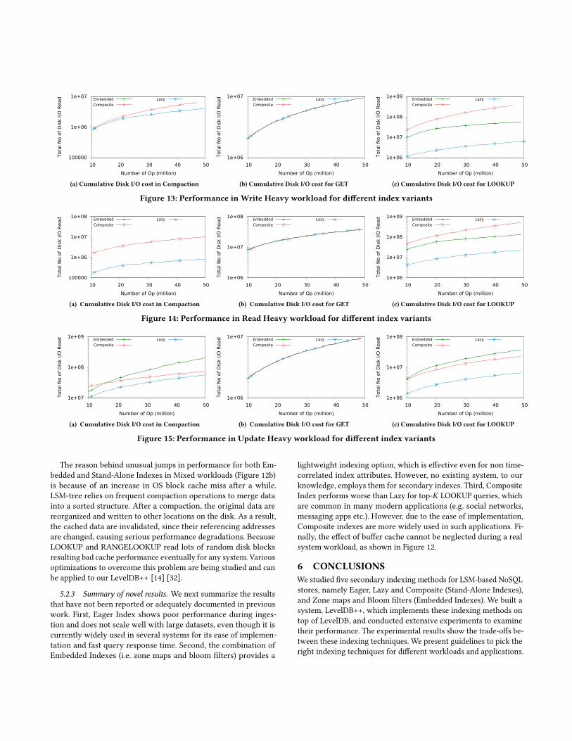
100000
1e+06
1e+07
10 20 30 40 50
Tota
l N
o o
f D
isk
I/O
Read
Number of Op (million)
Embedded
Composite
Lazy
(a) Cumulative Disk I/O cost in Compaction
1e+06
1e+07
10 20 30 40 50
Tota
l N
o o
f D
isk
I/O
Read
Number of Op (million)
Embedded
Composite
Lazy
(b) Cumulative Disk I/O cost for GET
1e+06
1e+07
1e+08
1e+09
10 20 30 40 50
Tota
l N
o o
f D
isk
I/O
Read
Number of Op (million)
Embedded
Composite
Lazy
(c) Cumulative Disk I/O cost for LOOKUP
Figure 13: Performance in Write Heavy workload for different index variants
100000
1e+06
1e+07
1e+08
10 20 30 40 50
Tota
l N
o o
f D
isk
I/O
Read
Number of Op (million)
Embedded
Composite
Lazy
(a) Cumulative Disk I/O cost in Compaction
1e+06
1e+07
1e+08
10 20 30 40 50
Tota
l N
o o
f D
isk
I/O
Read
Number of Op (million)
Embedded
Composite
Lazy
(b) Cumulative Disk I/O cost for GET
1e+06
1e+07
1e+08
1e+09
10 20 30 40 50
Tota
l N
o o
f D
isk
I/O
Read
Number of Op (million)
Embedded
Composite
Lazy
(c) Cumulative Disk I/O cost for LOOKUP
Figure 14: Performance in Read Heavy workload for different index variants
1e+07
1e+08
1e+09
10 20 30 40 50
Tota
l N
o o
f D
isk
I/O
Read
Number of Op (million)
Embedded
Composite
Lazy
(a) Cumulative Disk I/O cost in Compaction
1e+06
1e+07
10 20 30 40 50
Tota
l N
o o
f D
isk
I/O
Read
Number of Op (million)
Embedded
Composite
Lazy
(b) Cumulative Disk I/O cost for GET
1e+06
1e+07
1e+08
10 20 30 40 50
Tota
l N
o o
f D
isk
I/O
Read
Number of Op (million)
Embedded
Composite
Lazy
(c) Cumulative Disk I/O cost for LOOKUP
Figure 15: Performance in Update Heavy workload for different index variants
The reason behind unusual jumps in performance for both Em-
bedded and Stand-Alone Indexes in Mixed workloads (Figure 12b)
is because of an increase in OS block cache miss after a while.
LSM-tree relies on frequent compaction operations to merge data
into a sorted structure. After a compaction, the original data are
reorganized and written to other locations on the disk. As a result,
the cached data are invalidated, since their referencing addresses
are changed, causing serious performance degradations. Because
LOOKUP and RANGELOOKUP read lots of random disk blocks
resulting bad cache performance eventually for any system. Various
optimizations to overcome this problem are being studied and can
be applied to our LevelDB++ [14] [32].
5.2.3 Summary of novel results. We next summarize the results
that have not been reported or adequately documented in previous
work. First, Eager Index shows poor performance during inges-
tion and does not scale well with large datasets, even though it is
currently widely used in several systems for its ease of implemen-
tation and fast query response time. Second, the combination of
Embedded Indexes (i.e. zone maps and bloom filters) provides a
lightweight indexing option, which is effective even for non time-
correlated index attributes. However, no existing system, to our
knowledge, employs them for secondary indexes. Third, Composite
Index performs worse than Lazy for top-K LOOKUP queries, which
are common in many modern applications (e.g. social networks,
messaging apps etc.). However, due to the ease of implementation,
Composite indexes are more widely used in such applications. Fi-
nally, the effect of buffer cache cannot be neglected during a real
system workload, as shown in Figure 12.
6 CONCLUSIONSWe studied five secondary indexing methods for LSM-based NoSQL
stores, namely Eager, Lazy and Composite (Stand-Alone Indexes),
and Zone maps and Bloom filters (Embedded Indexes). We built a
system, LevelDB++, which implements these indexing methods on
top of LevelDB, and conducted extensive experiments to examine
their performance. The experimental results show the trade-offs be-
tween these indexing techniques. We present guidelines to pick the
right indexing techniques for different workloads and applications.

ACKNOWLEDGMENTSThis project is partially supported by NSF grants IIS-1447826 and
IIS-1619463, and a Samsungs GRO grant. The authors are grateful
to Abhinand Menon for helpful discussions and for building an
earlier version of the Twitter workload generator.
REFERENCES[1] Parag Agrawal, Adam Silberstein, Brian F Cooper, Utkarsh Srivastava, and Raghu
Ramakrishnan. 2009. Asynchronous view maintenance for VLSD databases. In
Proceedings of the 2009 ACM SIGMOD International Conference on Management ofdata. ACM, 179–192.
[2] Sattam Alsubaiee, Alexander Behm, Vinayak Borkar, Zachary Heilbron, Young-
Seok Kim, Michael J Carey, Markus Dreseler, and Chen Li. 2014. Storage Man-
agement in AsterixDB. Proceedings of the VLDB Endowment 7, 10 (2014).[3] Basho. 2017. Secondary Indexes in Riak. (October 2017). http://basho.com/posts/
technical/secondary-indexes-in-riak.
[4] Burton H Bloom. 1970. Space/time trade-offs in hash coding with allowable
errors. Commun. ACM 13, 7 (1970), 422–426.
[5] Fay Chang, Jeffrey Dean, Sanjay Ghemawat, Wilson C Hsieh, Deborah A Wal-
lach, Mike Burrows, Tushar Chandra, Andrew Fikes, and Robert E Gruber. 2008.
Bigtable: A distributed storage system for structured data. TOCS 26, 2 (2008), 4.[6] Brian F Cooper, Adam Silberstein, Erwin Tam, Raghu Ramakrishnan, and Russell
Sears. 2010. Benchmarking cloud serving systems with YCSB. In Proceedings ofthe 1st ACM symposium on Cloud computing. 143–154.
[7] James C Corbett, Jeffrey Dean, Michael Epstein, Andrew Fikes, Christopher Frost,
Jeffrey John Furman, Sanjay Ghemawat, Andrey Gubarev, Christopher Heiser,
Peter Hochschild, et al. 2013. Spanner: GoogleâĂŹs globally distributed database.
ACM Transactions on Computer Systems (TOCS) 31, 3 (2013), 8.[8] Debraj De and Lifeng Sang. 2009. QoS supported efficient clustered query pro-
cessing in large collaboration of heterogeneous sensor networks. In CollaborativeTechnologies and Systems, 2009. CTS’09. International Symposium on. IEEE, 242–249.
[9] Siying Dong, Mark Callaghan, Leonidas Galanis, Dhruba Borthakur, Tony Savor,
and Michael Strum. 2017. Optimizing Space Amplification in RocksDB.. In CIDR.[10] Robert Escriva, Bernard Wong, and Emin Gün Sirer. 2012. HyperDex: A dis-
tributed, searchable key-value store. ACM SIGCOMM Computer CommunicationReview 42, 4 (2012), 25–36.
[11] Facebook. 2017. Live Commenting: Behind the Scenes. (Oc-
tober 2017). https://code.facebook.com/posts/557771457592035/
live-commenting-behind-the-scenes/.
[12] A Feinberg. 2011. Project Voldemort: Reliable distributed storage. In Proceedingsof the 10th IEEE International Conference on Data Engineering.
[13] Lars George. 2011. HBase: the definitive guide. O’Reilly Media, Inc.
[14] Lei Guo, Dejun Teng, Rubao Lee, Feng Chen, Siyuan Ma, and Xiaodong
Zhang. 2016. Re-enabling high-speed caching for LSM-trees. arXiv preprintarXiv:1606.02015 (2016).
[15] Yuan He, Mo Li, and Yunhao Liu. 2008. Collaborative Query Processing Among
Heterogeneous Sensor Networks. In Proceedings of the 1st ACM InternationalWorkshop on Heterogeneous Sensor and Actor Networks (HeterSanet ’08). ACM,
New York, NY, USA, 25–30. https://doi.org/10.1145/1374699.1374705
[16] Todd Hoff. 2016. The Architecture Twitter Uses To Deal With 150M
Active Users, 300K QPS, A 22 MB/S Firehose, And Send Tweets In
Under 5 Seconds. (2016). http://highscalability.com/blog/2013/7/8/
the-architecture-twitter-uses-to-deal-with-150m-active-users.html.
[17] Aerospike inc. 2017. Aerospike Secondary Index Architecture. (October 2017).
https://www.aerospike.com/docs/architecture/secondary-index.html.
[18] Amazon Inc. 2017. Global Secondary Indexes - Amazon DynamoDB. (October
2017). http://docs.aws.amazon.com/amazondynamodb/latest/developerguide/
SecondaryIndexes.html.
[19] CouchDB Inc. 2017. CouchDB. (October 2017). http://couchdb.apache.org/.
[20] Facebook Inc. 2017. RocksDB. (October 2017). http://rocksdb.org/.
[21] Facebook Inc. 2017. Strategies to reduce write amplification. (October 2017).
https://github.com/facebook/rocksdb/issues/19.
[22] Google Inc. 2017. Google Snappy. (October 2017). http://google.github.io/snappy.
[23] Google Inc. 2017. LevelDB. (October 2017). http://leveldb.org.
[24] IBM Inc. 2017. IBM Big Data Analytics. (October 2017). https://www.ibm.com/
analytics/us/en/big-data/.
[25] IBM inc. 2017. Understanding Netezza Zone Maps. (October 2017).
https://www.ibm.com/developerworks/community/blogs/Wce085e09749a_
4650_a064_bb3f3b738fa3/entry/understanding_netezza_zone_maps?lang=en.
[26] MongoDB Inc. 2017. MongoDB. (October 2017). http://www.mongodb.com.
[27] Oracle Inc. 2017. Oracle: Using Zone Maps. (October 2017). http://docs.oracle.
com/database/121/DWHSG/zone_maps.htm.
[28] Teradata Inc. 2017. Teradata Teradata Analytics for Enterprise Applications.
(October 2017). http://www.teradata.com/analyticssolutions.
[29] Bettina Kemme and Gustavo Alonso. 2010. Database Replication: A Tale of
Research Across Communities. Proc. VLDB Endow. 3, 1-2 (Sept. 2010), 5–12.
https://doi.org/10.14778/1920841.1920847
[30] UCR Database Lab. 2017. Project website for open source code and workload
generator. (October 2017). http://dblab.cs.ucr.edu/projects/KeyValueIndexes/.
[31] Avinash Lakshman and Prashant Malik. 2010. Cassandra: A Decentralized Struc-
tured Storage System. SIGOPS Oper. Syst. Rev. 44, 2 (apr 2010), 35–40.[32] Lucas Lersch, Ismail Oukid,Wolfgang Lehner, and Ivan Schreter. 2017. An analysis
of LSM caching in NVRAM. In Proceedings of the 13th International Workshop onData Management on New Hardware. ACM, 9.
[33] Mahdi Tayarani Najaran and Norman C Hutchinson. 2013. Innesto: A searchable
key/value store for highly dimensional data. In CloudCom. IEEE, 411–420.
[34] Patrick O’Neil, Edward Cheng, Dieter Gawlick, and Elizabeth O’Neil. 1996. The
Log-Structured Merge-Tree (LSM-Tree). Acta Informatica 33, 4 (1996), 351–385.[35] Mohiuddin Abdul Qader and Vagelis Hristidis. 2017. Dualdb: An efficient lsm-
based publish/subscribe storage system. In Proceedings of the 29th InternationalConference on Scientific and Statistical Database Management. ACM, 24.
[36] Wei Tan, Sandeep Tata, Yuzhe Tang, and Liana Fong. 2014. Diff-Index: Differenti-
ated Index in Distributed Log-Structured Data Stores. In EDBT. 700–711.[37] Jianjun Zheng, Qian Lin, Jiatao Xu, Cheng Wei, Chuwei Zeng, Pingan Yang, and
Yunfan Zhang. 2017. PaxosStore: high-availability storage made practical in
WeChat. Proceedings of the VLDB Endowment 10, 12 (2017), 1730–1741.
AppendicesThe appendix is organized as follows. Appendix A reviews back-
ground on LSM-tree, LevelDB storage architecture and Bloom Fil-
ter. Appendix B provides pseudocode of LOOKUP (Ai , a, K) andRANGELOOKUP (Ai , a, b,K ) operation in LevelDB implementation
for different index variants. Appendix C presents supplementary
experimental results, which analyze the effect of bloom filter, com-
pression and concurrency on different secondary indexes. Appendix
D describes effect of distributed environment on secondary indexes.
A BACKGROUNDA.1 LSM tree
Figure 16: LSM tree components.
An LSM tree generally consists of an in-memory component
(level in LevelDB terminology) and several immutable on-disk com-
ponents (levels). Each component consists of several data files and
each data file consists of several data blocks. As depicted in Fig-
ure 16, all writes go to in-memory component (C0) first and then
flush into the first disk component once the in-memory data is over
the size limit of C0, and so on. The on-disk components normally
increase in size as shown in Figure 16 from C1 to CL. A background
process (compaction) will periodically merge the smaller compo-
nents to larger components as the data grows. Delete on LSM is
achieved by writing a tombstone of the deleted entry to C0, which
will later propagate to the component that stores this entry. LSM
is highly optimized for writes as a write only needs to update the
in-memory component C0. The append-only style updates mean
that an LSM tree could contain different versions of the same entry
(different key-value pairs with the same key) in different compo-
nents. A read (GET) on an LSM tree starts from C0 and then goes to
C1, C2 and so on until the desired entry is found, which makes sure
the newest (valid) version of an entry will be returned. The older

versions of an entry (either updated or deleted) are obsolete and
will be discarded during the merge (compaction) process. Conven-
tionally, the in-memory component (C0) is referred asMemTableand the on-disk components are referred as SSTable.
A.2 SSTable in LevelDB
Figure 17: LevelDB SSTable structure.
Here we present some storage details of LevelDB [23] as back-
ground for ease of understanding of the paper. Level-(i + 1) is 10times larger than level-i in LevelDB. Each level (component) con-
sists of a set of disk files (SSTables), each having a size around 2
MBs. The SSTables in the same level may not contain the same key
(except level-02). Further, LevelDB partitions its SSTables into data
blocks (normally tens of KB in size). The format of an SSTable file
in LevelDB is shown in Figure 17. The key-value pairs are stored in
the data blocks sorted by their key. Filter Meta blocks store a bloom
filter for each block, computed based on the keys of the entries in
that block, to speedup GET operations. Then, there are data index
blocks, which we call zone maps for primary table.
A.3 Bloom FilterBloom filter [4] is a hashing technique to efficiently test if an item is
included in a set of items. Each item in the set is mapped to several
bit positions, which are set to 1, by a set of n hash functions. Then,
the bloom filter of a set is the OR-ing of all these bitstrings. To check
the membership of an item in the set, we compute n bit positions
using the same n hash functions and check if all corresponding
bits of the bloom filter are set to 1. If no, we return false, else we
have to check if this item exists due to possible false positives.
The false positive rate depends on the number of hash functions
n, the number of items in the set S and the length of the bit arrays
m, which can be approximately computed as Equation 1. Given
S andm, the minimal false positive rate is 2−mS ln2 by setting the
n = mS ln2. (
1 −[1 − 1
m
]nS )n≈
(1 − e−nS/m
)n(1)
B ALGORITHMSIn all algorithms, we assume each tuple(k,v) is associated with
a sequence number (seq). We show how we add the records on
Min-Heap H based on this seq in Algorithm 1. Algorithm 2, 3, 4,
5 present the pseudocodes of LOOKUP(Ai , a, K) in Stand-Alone
Eager, Lazy, and Composite Index and Embedded Index respectively.
2which is C1 in Figure 16 as LevelDB does not number the memory component
Algorithm 6, 7,8 present the pseudocodes of RANGELOOKUP(Ai ,a, b, K ) in Stand-Alone Lazy, and Composite and Embedded Index
respectively. Stand-Alone Eager Index uses existing range query
API for primary key on the Stand-Alone Index Table in LevelDB.
Algorithm 1 Min-Heap H .Add(K , ⟨k,v⟩) Procedure1: if H .size () == K ∧ H .top.seq < ⟨k,v⟩.seq then2: H .pop ();3: H .put(⟨k,v⟩);4: else if H .size () < K then5: H .put(⟨k,v⟩);6: return
Algorithm 2 LOOKUP Procedure using Eager Index
1: Create Min-Heap H;
2: Primary key list L← return of GET(a) on index table Ti . {Sup-pose the order is maintained as recent key to older keys}
3: for k in L do4: ⟨k,v⟩ ← return of GET(k) on data table.
5: if v .val (Ai ) == a then6: H.add(K , ⟨k,v⟩) {Algorithm 1}
7: if H .size () == K then8: BREAK
9: return List of pairs in H
Algorithm 3 LOOKUP Procedure using Lazy Index
1: Create Min-Heap H;
{starts from MemTable (C0) and then moves to SSTable, C1 is
LevelDB’s level-0 SSTable.}
2: for j from 0 to L do3: if val (Ai ) is not in Cj then4: NEXT
5: List of primary keys P ← val (Ai ) in Cj6: for k in P do7: ⟨k,v⟩ ← return of GET(k) on data table.
8: if v .val (Ai ) == a then9: H.add(K , ⟨k,v⟩) {Algorithm 1}
10: if H .size () == K then11: return H12: return List of pairs in H
C SUPPLEMENTARY EXPERIMENTSC.1 Effects of varying bloom filter lengthsThe length of each bloom filter used in Embedded Index also has
effect on LOOKUP performance in two folds: (1) with larger bloom
filter, the false positive rate will drop thus the number of blocks to
be loaded into memory is smaller, and (2) the cost of checking each
bloom filter is higher because more hash functions are applied for
each key to check its existence as the bloom filter length increases.
We conducted the experiment by varying the value of bits per keyfrom 20 to 1000 with our seed twitter dataset to determine the
optimal choice of bloom filter length for this dataset. We write 20

0.1
1
10
100
1000
10000
100000
1e+06
1e+07
Embedded vs Embedded-NC Lazy vs Lazy-NC Composite vs Composite-NC
Tim
e p
er
Op (
mill
iseco
nds)
Topk=10
0.1
1
10
100
1000
10000
100000
1e+06
1e+07
Embedded vs Embedded-NC Lazy vs Lazy-NC Composite vs Composite-NC
Tim
e p
er
Op (
mill
iseco
nds)
Topk=No Limit
(a) LOOKUP Response Time
0.1
1
10
100
1000
10000
100000
1e+06
1e+07
Embedded vs Embedded-NC Lazy vs Lazy-NC Composite vs Composite-NC
Tim
e p
er
Op (
mill
iseco
nds)
Topk=10
0.1
1
10
100
1000
10000
100000
1e+06
1e+07
Embedded vs Embedded-NC Lazy vs Lazy-NC Composite vs Composite-NC
Tim
e p
er
Op (
mill
iseco
nds)
Topk=No Limit
(b) RANGELOOKUP Response Time (Selectivity: 10)
Figure 18: UserID Index performance for different variants with and without compression. (NC = Not Compressed)
Algorithm 4 LOOKUP Procedure using Composite Index
1: Create Min-Heap H;
{starts from MemTable (C0) and then moves to SSTable, C1 is
LevelDB’s level-0 SSTable.}
2: for j from 0 to L do3: it ← SSTable :: Iterator j .SEEK (a)4: while it .valid() do5: Composite key, ckey ← it .key()6: skey ← ckey.ExtractSecondarykey()7: if a == skey then8: k ← ckey.ExtractPrimaryKey()9: ⟨k,v⟩ ← return of GET(k) on data table.
10: if v .val (Ai ) == a then11: H.add(K , ⟨k,v⟩) {Algorithm 1}
12: else if skey > a then13: BREAK
14: it .NEXT ()15: return List of pairs in H
Table 8: How LOOKUP performance, average false positiverates and database size vary with bloom filter length
Bits Per Key DB Size (MB) False Positive % Mean LOOKUP Latency(Milliseconds)
20 10,127 0.64% 52
50 10,256 0.44% 49
100 10,470 0.08% 21
200 10,899 0.08% 20.5
500 12,186 0.08% 22
1000 14,325 0.08% 32
million tweets with Embedded Index on UserID and performed 200K
LOOKUPs. Table 8 shows the average performance of LOOKUPs.
Here we see that the LOOKUP performance starts to increase with
increasing bits per key setting of bloom filter (20 to 200) as the
false positive rate decreases. But then the performance decreases
with larger value of bits per key where the false positive rate is low
enough, but the cost of checking bloom filters increases. We also
show the space trade-offs in Table 8. As the bits per key increases,
the bloom filter takes more space. In our experiments, we set bits
per key as 100, because the LOOKUP performance is very close to
setting it as 200 to 300 but with reasonable space overhead.
C.2 Effect of compression on indexes
20
40
60
80
100
120
Embedded Composite Lazy
Tim
e p
er
Op (
µs)
CompressedNot Compressed
Figure 19: Mean Time per PUT operation on UserID index
In this section, we report how block compression affects sec-
ondary index’s performance. Keeping same experimental settings
and same dataset from Section 5, we rebuild our secondary indexes
for UserID index without compression and perform top-K LOOKUP
and RANGE LOOKUP queries. Figures 18a and 18b show varying
top-K LOOKUP and RANGELOOKUP query response times of dif-
ferent secondary indexes, for default Snappy compression [22] en-
abled against no compression. We see the same relationship exists
between different indexing variants with or without compression.
But LOOKUP and RANGELOOKUP response times are slightly
higher for all of them if there is no compression enabled. Figure 19
shows that we also get almost identical results for PUT performance
for all secondary indexes with and without compression.
C.3 Effect of multi-threaded environmentIn this section, we report our secondary index’s performance in
multi-threaded environment. We repeat LOOKUP and RANGE
LOOKUP queries from Section 5 on UserID index and measure
throughput (i.e. number of operation per hour) varying number
of concurrent threads. Top-K is set as 10. Figure 20 shows that
secondary indexes show same relationship between them for multi-
threaded environment compare to single thread. Stand-Alone In-
dexes has slightly higher throughput for high concurrencies over
Embedded Index because different threads can efficiently access
data and index table in parallel. Although, we see that increasing

Algorithm 5 LOOKUP Procedure using Embedded Index
1: function GetLite (key, level)2: for l = 0→ L do3: if l .SEEK(key) == True then4: if l = level then5: return True {SEEK operation Checks only in-memory
metadata, index block and bloom filters for primary key
to lookup key}
6: else7: return False
1: function LOOKUP (Ai , a, K )2: Create Min-Heap H;
3: for table in MemTable do4: for ⟨k,v⟩ in table do5: if val (Ai ) == a then6: H.add(K , ⟨k,v⟩) {Algorithm 1}
7: if H .size () == K then8: return List of K pairs in H
9: for l = 0→ L do10: for sstablej in level-l do11: if sstablej .дlobalzonemap (Ai ) .contains (a) == True
then12: for block bm in sstablej do13: if bm .bloomf ilter (Ai ) .contains (a) == False or
bm .zonemap (Ai ) .contains (a) == False then14: NEXT
15: load bm of sstablej in memory;
16: for ⟨k,v⟩ in bm do17: if v .val (Ai ) .equals(a) ∧ GetLite(k, l) == True
then18: H.add(K , ⟨k,v⟩) {Algorithm 1}
19: if H .size () == K then20: return List of K pairs in H21: return List of pairs in H
10
100
1000
10000
100000
Embedded Lazy Composite
Thro
ug
hp
ut:
No o
f O
p p
er
Hour
No of Threads: 1No of Threads: 3
No of Threads: 5
(a) LOOKUP Throughput
1
10
100
1000
10000
100000
Embedded Lazy Composite
Thro
ug
hp
ut:
No o
f O
p p
er
Hour
No of Threads: 1No of Threads: 3
No of Threads: 5
(b) RANGELOOKUP Throughput
Figure 20: UserID Index performance for multi-threads
the number of threads does not necessarily increase throughout
much (even decrease throughput in some cases) as different threads
compete with each other for system resources (e.g. database com-
ponents) and eventually decrease system throughput.
D EFFECT OF DISTRIBUTED ENVIRONMENTThe main overhead of a distributed NoSQL environment is the cost
of maintaining the replication consistency [29]. In this paper, we
focus on the storage engine module, which can be conceptually
Algorithm 6 RANGELOOKUP Procedure using Lazy Index
1: Create Min-Heap H;
{starts from MemTable (C0) and then moves to SSTable, C1 is
LevelDB’s level-0 SSTable.}
2: for j from 0 to L do3: it ← SSTable :: Iterator j .SEEK (a)4: while it .valid() do5: if it .key() in [a,b] then6: List of primary keys P ← it .value()7: for k in P do8: ⟨k,v⟩ ← return of GET(k) on data table.
9: if v .val (Ai ) == it .key() then10: H.add(K , ⟨k,v⟩) {Algorithm 1}
11: else12: BREAK
13: it .NEXT ()14: return List of pairs in H
Algorithm 7 RANGELOOKUP Procedure using Composite Index
1: Create Min-Heap H;
{starts from MemTable (C0) and then moves to SSTable, C1 is
LevelDB’s level-0 SSTable.}
2: for j from 0 to L do3: it ← SSTable :: Iterator j .SEEK (a)4: while it .valid() do5: Composite key, ckey ← it .key()6: skey ← ckey.ExtractSecondarykey()7: if skey in [a,b] then8: Repeat← Line 8-12 from Algorithm 4
9: else if skey > b then10: BREAK
11: it .NEXT ()12: return List of pairs in H
Algorithm 8 RANGELOOKUP Procedure using Embedded Index
1: Create Min-Heap H;
2: for table in MemTable do3: for ⟨k,v⟩ in table do4: if v .val (Ai ) in [a,b] then5: H.add(K , ⟨k,v⟩) {Algorithm 1}
6: if H .size () == K then7: return List of K pairs in H
{REPEAT LINE 9 to 20 from Algorithm 5 to populate H, but
replace contains(a) function with intersects(a,b) and equals(a)withwithin(a,b)}
8: return List of pairs in H
viewed as a state machine maintained by any consensus protocol-
based (e.g. Paxos, Raft) replication engine (e.g. PaxosStore [37]). The
overhead of the replication engine generally does not depend on the
choice of the implementation of the state machine (i.e. implementa-
tion of secondary indexes). The other aspects of distributed envi-
ronment (i.e. partitioning module, cluster membership etc.) can also
be designed independent to the storage engine module [31] [2] [3].