A Comparison of Stated and Revealed Preference Methods for

A Comparison of Stated and Revealed Preference Methods for FisheriesManagement

by

Robert L. Hicks

American Agricultural Economics Association2002 Annual Meeting, July 28-31, 2002, Long Beach, California

Selected Paper

A Comparison of Stated and Revealed Preference Methods for Fisheries Management

10 May 2002

Robert L. Hicks

Department of Coastal and Ocean Policy

Virginia Institute of Marine Science

The College of William and Mary

PO Box 1346

Gloucester Point, VA 23062

804.684.7822, [email protected]

Copyright 2002 by Robert L. Hicks. All rights reserved. Readers may make verbatim copies of this document for non-commercial purposes by any means, provided that this copyright notice appears on all such copies.

Draft: Do not cite without permission of author.

2

I. Introduction

Environmental managers are becoming increasingly aware that environmental policies

must be crafted in a way that incorporates the human dimensions of the ecosystem. Failure to

incorporate stakeholder preferences into management measures can lead to policies that fail

because people’s preferences, motivations, and behavior concerning their use and impact on the

environment were not properly considered even if defensible natural science approaches were

incorporated in the management decision. In this paper we explore two methodologies for

quantifying people’s preferences for environmental goods and management: stated and revealed

preference methods.

The stated preference method we use, termed the Stated Preference Discrete Choice

technique has been applied to a wide variety of settings including market research for marketed

goods including appliance choice (Ben-Akiva et al.), yogurt (Guadagni et al.), and light-rail

transportation (Preston). The technique is a particular form of conjoint analysis, which has broad

application to measuring preferences for both market and non-market goods. For resource

managers, the method potentially enables the exploration of new policy tools, non-observable

ranges for management tools, and examination of policies with multiple attributes. The stated

preference discrete choice technique relies on respondents making choices over hypothetical

scenarios. Respondents are asked to choose the ‘best’ alternative from among a set of

hypothetical scenarios, which are completely described by a set of attributes generated from an

experimental design.

Conversely, Revealed Preferences techniques use observations on actual choices made by

people to measure preferences. The primary advantage of the Revealed Preference technique is

the reliance on actual choices, avoiding the potential problems associated with hypothetical

responses such as strategic responses or a failure to properly consider behavioral constraints. The

strength of Revealed Preference techniques is also its primary weakness. By relying on

observable trips, analyses are largely limited to observable states of the world. Therefore,

Revealed Preference techniques may not be suitable for quantifying preferences for attributes

where no variation exists or for which the attribute cannot be observed.

For the application considered here, management of recreational angling for summer

flounder (Paralichthys denatus) in the Northeastern United States, there is a near lack of variation

with respect to actual management policy (see Table 1) complicating the recovery of behavioral

parameters. Summer flounder is one of the most sought after recreationally caught fish along the

eastern seaboard of the United States. It is typically in the top three species in terms of anglers


3

targeting it per year (National Marine Fisheries Service). Scientists have for some time been

concerned with the overall exploitation level of summer flounder by both commercial and

recreational fishermen along the middle Atlantic coast. Managers responsible for the stock have

gradually been tightening regulations in an effort to conserve the stock of summer flounder.

Because of the lack of variation in observed management, we employ the Stated

Preference Discrete Choice technique to capture information about preferences for fisheries

management options. To identify behavioral responses for environmental conditions for which

there is observable variation (such as catch conditions), the Revealed Preference approach is

used. Taken together, these two approaches can be used to ‘enrich’ the preference model so that

preferences for all relevant choice attributes can be captured. Combining the two approaches also

allows for rigorous hypothesis testing for consistency across the two models, including the

consistency of parameter, welfare, and other policy-relevant estimates across the two

methodologies. These issues are important in order to discern whether hypothetical responses

offer useful information in an environmental management setting. Our findings suggest that

while the two methods offer very similar yet statistically different results, policy relevant outputs

(e.g. welfare measures and estimates of participation change) are remarkably consistent across the

models.

The organization of the paper will proceed as follows. We will review the literature

important for combining revealed and stated preference analyses (Section II), describe the data

collection and experimental design (Section III), present models of angler behavior (Section IV),

discuss results and application to evaluating policy (Section V), and conclude with a summary of

findings with recommendations for future SPDC studies (Section VI).


4

Table 1. Summer Flounder Regulations, 20001

State Minimum

Size Limit (inches)

Possession

Limit

Open Season

Massachusetts 15.5 8 May 10 - Oct. 2

Rhode Island 15.5 8 May 10 - Oct. 2

Connecticut 15.5 8 May 10 - Oct. 2

New York 15.5 8 May 10 - Oct. 2

New Jersey 15.5 8 May 6 - Oct. 20

Delaware 15.5 8 May 10 - Oct. 2

Maryland Bays 15 8 May 15 - Dec. 31

Maryland Coastal 15.5 8 April 15 - Dec. 11

Potomac River 15.5 8 May 15 - Dec. 31

Virginia 15.5 8 March 29 - July 23

Aug. 2 - Dec. 31

North Carolina 15.5 8 Jan. 1 - Dec. 31

Source: Atlantic States Marine Fisheries Commission, personal correspondence, May 14, 2001.

II. Related Literature

To date, the revealed preference approach (hereafter referred to as RP), has been used in

a variety of settings related to environmental valuation (Bockstael et al. [1989], Bockstael et al.

[1991], and Hicks ) and environmental management (Kaoru, Kaoru and Smith, McConnell et al.,

Pendleton, and Schumann). The revealed preference approach uses information collected about

actual choices made by individuals to estimate statistical models of recreation demand. For

recreational fishing trips the model captures tradeoffs with regard to expected catch, cost of travel

to site, management regulations, environmental conditions, and other factors deemed important to

describe recreational site choice. The model allows preferences to be quantified so that

management options can be ranked and the value of changing environmental conditions can be

calculated (e.g. the value of recreational fishing, or the loss to recreational anglers due to an oil

spill).

1 For the period 1996-1998, there was even less variation in regulations: there were no closed seasons and the same minimum size and possession limits. Minimum size limits ranges were from 14 to 15 inches and possession limits ranged from 8 to 10 fish.


5

The RP methodology relies on variation in the natural environment so that the statistical

model can discern how the various factors important for describing recreational site choice

influence the choice. If no variation is found in the data (e.g. water quality is uniformly

distributed) then the model will fail to quantify the effect of that factor. The aforementioned

example of recreational angling for summer flounder in the Northeastern United States is an

example where the management-relevant attributes (e.g. bag limits, size limits, and open seasons)

are set uniformly across states.

Discrete choice RP approaches, based upon observable data at a site, are limited to

analyzing the affect of actual factors at a site. For example, if managers were considering new

management tools such as property right regimes, then current behavior would provide little

information about preferences if choices were not made in the context of property right

management regimes. Therefore, revealed preference approaches may be limited in its

application to many environmental problems.

Stated preference techniques rely on angler’s responses to hypothetical scenarios. For

example, the researcher might describe a hypothetical fishing trip to an angler and ask the angler

whether they would take the trip or not. Stated preference techniques have two major classes of

elicitation techniques to get at angler’s preferences for fisheries management. The first type,

contingent valuation, measures the value of a change from the status quo to some other state of

the world (Mitchell and Carson). For example, one might ask anglers to consider their current

trip and ask them their willingness to pay to avoid a decrease in water quality, to quantify the

economic loss of going to a more restrictive management position. For our problem, the

technique is not well suited to measuring preferences for all of the attributes of the fishing

experience (expected catch, cost of travel to site, management regulations, environmental

conditions, etc.) since typically very few attributes are varied over questions. However, the

technique is useful for exploring new management tools or examining willingness to pay in the

context of tightening or loosening regulations.

Another stated preference methodology, Stated Preference Discrete Choice (SPDC)

techniques first attributed to Louviere et al. have been applied to environmental management

problems such as Alaska fishing (Lee), hunting in Canada (Louviere et al.), and Salmon Fishing

(Boyle et al.). Like contingent valuation, SPDC techniques applied to fishing management gain

information about preferences by analyzing responses to hypothetical fishing trips. Further,

SPDC considers a fishing trip as a bundle of attributes describing a trip (along the lines of

Lancaster’s [1966, 1971] idea of a good as being defined by a collection of attributes). Using

experimental design techniques, anglers are given trip comparisons that are optimal in the sense


6

that they require the respondent to make tradeoffs across the different trip attributes

simultaneously. Therefore, it is possible to examine how preferences for a management measures

such as bag limits might change as other management changes, as environmental conditions

change, or as the cost of the trip changes.

Additionally, new policy-relevant attributes can be examined; for example, anglers might

be asked to consider a trip under the existing management regime and one with a new

management tool in place (for example, gear or area restrictions). Like contingent valuation,

SPDC is based upon hypothetical, not real behavior. Consequently, questions could be raised

about the veracity of results based upon this type of data.

There is a growing body of literature comparing revealed and stated preference methods.

The primary idea behind combining revealed and stated preference data is to enrich the choice

model so that the reality of choice is grounded in information about observed choices while

exploring new or out-of-range alternatives using hypothetical choices. This literature has focused

on testing for parameter homogeneity across the two models (Swait et al., Adamowicz et al.

[1994], Adamowicz et al. [1997], and Guadagni et al.). These tests are seen as validity tests for

the SPDC method so that policy guidance resulting from the SPDC model will be relevant for

real-world application. There is little guidance in the use of SPDC methods when tests for

parameter homogeneity fail. For these cases, Louviere et al. suggest that these issues are largely

unresolved. Because the SPDC design matrices are almost always better conditioned than their

RP counterparts, use of SPDC may be defensible for cases of partial or perhaps complete

rejection of parameter homogeneity of parameters. In this paper, we explore these issues and

examine difference in policy-relevant outputs from models derived from RP data and those from

SPDC data.

III. Data and Experimental Design

The collection of RP and SPDC data involved an approach that combined field-intercept

and mail surveys of recreational anglers in the Northeastern United States. Because the SPDC

method relies so heavily on the instrument, information conveyed, the attributes, and the

experimental design, the data collection step of the research project is a vitally important process.

For this line of research, over one year of effort was expended to refine the survey instrument to

the greatest degree possible. Numerous pre-test instruments were examined for respondents in

the National Marine Fisheries Service. In 1999, a field test was undertaken in Ocean City,

Maryland. Based upon feedback on this field test, it was decided that the intercept survey

(described in Hicks) should be used to collect RP data on respondents (as it had been used in the


7

past), and then a mail follow-up could be conducted to obtain SPDC data for intercepted

fishermen agreeing to participate in the follow-up mail survey.

Four focus groups were held in Baltimore Maryland during March 2000. The goal of the

focus group was to finalize the survey instrument. All portions of the survey going into the focus

group were under consideration for change as a result of feedback from the respondents.

Respondents were also asked about ranges of attributes, including the cost of the trip, the level of

catches for summer flounder, etc. Additionally, respondents were probed about the appearance of

the survey and cover letter, as well as how effective it conveyed information to the reader. These

steps were taken to insure as high a response rate as possible. Without doubt, the greatest focus

was on the SPDC questions themselves. Respondents were probed as to their understanding of

attributes, missing attributes, and definitions used in the study.

After analyzing the results of the focus group, it was found that even with such a small

sample, the model performed quite well with regard to sign and significance of coefficients. The

final list of attributes was chosen based upon two presiding considerations. First and foremost,

attributes were chosen and defined to make the hypothetical trip comparison meaningful for

anglers. Additionally, attributes were defined to make the comparison consistent with the RP

models that have been used in past studies. Following feedback from the focus group, the

questionnaire was finalized in March of 2000. Table 2 contains the final attributes, definitions,

and levels used in the SPDC mail survey.


8

Table 2. Final Attributes, Definitions, and Ranges for SPDC Survey

Attribute Definition Ranges Cost of traveling to a site

Includes gas, wear and tear on your vehicle and other expenses you might have from traveling to and from a fishing access site (such as tolls, ferry fees, and parking fees). This cost also includes expenses for food, ice, and fishing equipment used on this trip. The cost does not include guide or boat fees.

{$5, $20, $30, $40,

$55}

Bag limit for summer flounder

The most summer flounder an angler can legally keep per day of fishing.

{1, 4, 6, 8, 12}

(fish) Minimum size limit for summer flounder

Summer flounder smaller than a minimum size limit must be released.

{12, 14, 15, 16, 18}

(inches)

Likely catch of summer flounder

Anglers never know exactly how many summer flounder they will catch when they take a trip. However, they often have an idea of how many fish they are likely to catch.

{2, 5, 8, 11, 14}

(fish)

Likely fishing success for all other species

When taking a trip, anglers might also be interested in catching species besides summer flounder. Fishing success refers to the expected number of fish caught for all other species that you might encounter for a typical trip in your area.

{Below Average,

Average, Above Average}

Likely Number of summer flounder of legal size

Anglers also are never sure of the size of summer flounder they will catch. However, they often might be aware of differences in locations that might lead to differences in the sizes of fish caught.

{0, 1, 3, 6, 10}

(fish)

Once the attributes and attribute levels were finalized, the final design needed to be

created. Based upon our feedback from focus groups and other survey pre-test, it was determined

that respondents should only receive four of the SPDC questions. This level was determined

because of two reasons: 1) survey fatigue might lead to ‘poor’ responses if any more SPDC

questions were offered to them and 2) for each two SPDC questions added, the survey is

lengthened by one page. Any lengthening of the survey might signal to respondents that the

survey might be too time consuming to complete. Upon opening a package, the primary indicator

of how much time a survey will take to complete is the size and thickness of the instrument. The

two factors taken in combination led us to the conservative number of four SPDC trip

comparisons per respondent.

Given these constraints, the challenge was to design a choice experiment that captures

preferences for fisheries management tools and the other attributes identified in the pre-test and


9

focus group steps. Since each respondent was getting a relatively low number of SPDC

questions, we decided to divide the survey into blocks (or unique version of the survey), with

each block having different levels of attributes for the four trip comparisons. A Type V

resolution design was chosen as a first effort at the design matrix, ensuring that all main and cross

effects for attributes in the model could be estimated. The next step was to pair down the

candidate design into the best design possible given the fact that we were limited to 4 (questions)

x 18 (unique sets of questionnaires)= 72 unique trip comparisons.

Clearly, increasing the number of blocks increases the efficiency of the design matrix

since increasing the number of unique trip comparisons allows for more tradeoffs by respondents.

However, increasing the number of blocks increases survey cost because each respondent is

tracked during several stages of the mailing the survey according to their assigned block

(described below). Given the constraints on blocks and questions per block, the final design was

chosen from the candidate design using an algorithm that searched over the design space. The

optimal design was chosen based upon D optimality, which seeks to find the design that

maximizes the determinant of the design matrix ( XX ′max ). In effect, choosing a design

matrix on the basis of D optimality finds the design that best captures trade-offs across the

included factors.

Figure 1 shows an example of one of the actual trip comparisons from the final design

used in the SPDC instrument. Respondents were asked:

“Suppose last August that you could have chosen only from the recreational opportunities

described below.Please review the trip descriptions and answer the two questions at the bottom of

the table.”

After respondents viewed the three options, they were asked to indicate “Which trip do you most

prefer.” All respondents were asked to consider the choice of trips relative to August 1999. This

was done to anchor all respondents to the same time period versus adding time period explicitly

as an additional attribute in the choice. August was chosen because it is the generally the peak

season for summer flounder fishing. This setup was chosen to avoid having respondents during

the periods in either early spring or late December getting an instrument whose catch ranges were

not believable.


10

Figure 1. An actual SPDC trip comparison.

A booklet very close to the size recommended by Dillman was prepared for the mail

survey. A modified Dillman method was used to maximize the survey response rate (Table 3).

The first step was to recruit field intercept respondents at the time of the field survey. Once

respondents agreed to participate in the follow-up survey they were given a survey brochure that

very briefly described that they would soon receive a mail survey that would help the NMFS

know more about what they thought about fisheries management. It was a full-colored tri-fold

brochure that was primarily designed to help respondents recall that they had agreed to participate

at the time of opening the mail survey (this brochure is available from the author).


11

Table 3. Mail survey steps and response rates

Action Time Administered

Survey Brochure At time of field intercept

First mailing No more than one month after intercept

Post Card Two weeks after the mailing of the First Mailing

Second Mailing Two weeks after mailing of the Post card

Overall response rates2

Months

Response Rate

Wave 2 March-April 58.4%

Wave 3 May-June 56.3%

Wave 4 July-August 55.7%

Wave 5 September-October 59.6%

Wave 6 November-December 53.5%

Average Response Rates 56.8%

At the end of each month, a sub-sample of intercepted anglers who agreed to participate

in the SPDC survey were mailed the survey instrument along with a cover page that reiterated

many of the points made in the survey brochure and reinforced the notion that each respondent’s

opinion mattered3. Following a two-week period, respondents who had not yet responded to the

first mail survey were sent a postcard reminder that reinforced the points made in earlier cover

letters and brochures. If after two weeks from the date of mailing the postcard, respondents had

still not returned a survey, a second survey was sent to them along with a slightly different cover

letter that contained similar points as previous information, but in slightly more forceful

language. Prior to the beginning of the initial mailing each survey respondent was randomly

assigned a survey version (also referred to as a block). A database tracked all subsequent

mailings to individuals according to their block number. This ensured that if the second mailing

were necessary, respondents would receive the same version of the survey across mailings.

2 Incorrect addresses are not included in the calculation of response rates. For the entire survey, there were 5009 surveys sent out of which 150 were undeliverable addresses. 3 Anglers were sub-sampled according to the MRFSS sample allocation within states, waves, and method of fishing.


12

IV. Model of Angler Behavior

Both the RP and SPDC model employs discrete choice statistical techniques to estimate

models of behavior. The discrete choice technique assumes that anglers must choose between a

number of discrete alternatives. Each alternative is comprised of attributes associated with that

alternative. For models of recreational angling, the discrete alternatives are often assumed to be

fishing sites, and the angler’s vector of site-specific attributes, X, is typically assumed to be

populated by data such as the cost of traveling to the site, indications of the site’s fishing quality,

and other site-specific attributes. In the discrete choice framework, the angler is assumed to

choose the site i from among a set of sites S that maximizes the angler’s utility. Assume that the

angler’s indirect utility function for site i is given by

iii ),(v),(V ε+β=β XX (1)

where Xi is the vector of site and individual-specific attributes associated with site I, β is a vector

of parameters on the observable portion of the individual’s indirect utility function, ),(v iXβ .

Finally, iε is the unobservable portion of the individual’s indirect utility function and is assumed

to be site specific. The angler then compares all potential choices in his choice set, S, and

chooses the best site, i:

Si,Sj ),(V),(V ji ∈∈∀β>β XX (2)

The challenge is to take the model given by (1) and (2) and develop a statistical model

that will enable the recovery of the behavioral parameters, β. Of course, the structure of the

model will depend heavily on assumptions about the form of the site-specific error term, iε . In

this paper, we use two forms of the error structure, the Generalized Extreme Value distribution

(GEV)4 and the more restrictive independent logit. The independent logit specification specifies

the probability of choosing site i as

∑∈

β

β

=

Sj

)j,(v

)i,(v

e

e)i(obPr X

X

(3)

Recent work using revealed preference techniques have attempted to provide information

that is useful for management and able to analyze issues that are species-specific (Schumann,

Jones and Lupi, and Hicks and Steinback). Findings for these models are twofold:

4 For brevity, the nested stated preference discrete choice model, which first models participation and conditional on participation site choice, will not be presented in the text.


13

1) If management measures or stock conditions change at a species-specific

level, then species-specific models of angler behavior are important to

develop, and

2) Species-specific models using RP data are very hard or impossible to

estimate because of the large number of species targeted and caught by

marine anglers, management measures do not vary much for a particular

species, and data requirements to characterize fishing quality for all sites

on a species-by-species basis are burdensome.

With these two factors in-play, it was clear that developing a useful summer flounder

model would be at best very difficult to implement. Attempts to estimate the discrete choice RP

model with bag and size limits explicitly included as factors in the model failed because of a near

complete lack of variation in the management data. Therefore, we developed a simpler RP model

that enabled anglers to substitute between summer flounder and other species they may want to

target. We assume that anglers choose sites based upon all species regardless of what they

choose to target. Consequently, they are concerned with fishing quality for summer flounder as

well as the fishing quality for all other species they could catch at the site. Additionally, anglers

are concerned about the cost of taking a trip to site i.

It was decided to choose a simple choice structure to make the RP model as close to the

SPDC model as possible, making the statistical comparison as transparent as possible. The RP

variable definitions are given in Table 4. The overall goal in developing the RP model was to

estimate a model that would be useful to enrich the SPDC experiment and to test for parameter

homogeneity across the two techniques.

Table 4. RP Variable Definitions.

Variable Name Definition

TC_RP i Travel Cost based on RP data to Site i. Equals roundtrip

distance to site i times the rate of $0.33 per mile.

SF_RPi Average Catch per trip per wave at site i for summer flounder

based on RP data. Average taken over the period 1997-2000.

OC_RPi Average Catch per trip per wave at site i for all other species

based on RP data. Average taken over the period 1997-2000.

The definition of the indirect utility function is defined as follows:

iiiirpi rp_oc*oc_rp_brp_sf*sf_rp_brp_tc*tcost_rp_b),(V ε+++=β X (1’)


14

and the parameters to be estimated are given by b_rp_tcosti, b_rp_sfi, b_rp_oci. Notice that this

indirect utility function is linear with regard to the travel cost coefficient. This assumption

ensures a closed form solutions for the welfare estimates that follow. Estimating more elaborate

versions of (1’) are beyond the scope of this paper but have been explored elsewhere (see Layton

and Kling and Herriges). For the RP model, we assume a non-nested choice structure by

estimating a multinomial logit model using maximum likelihood techniques.

It should be noted that the parameters listed in (1’) can be rewritten as follows:

{ } { }co_rp_b,fs_rp_b,tcost_rp_boc_rp_b,sf_rp_b,tcost_rp_b ′λ′λ′λ=

The parameter λ, referred to as the scale factor, is tied directly to the data source from which the

data is estimated. The parameter λ is inversely related to the variance of the error term in the

model (Louviere et al.) and is impossible to identify if only estimating model (1’). For this

reason, most applications of discrete choice models do not explicitly include the scale factor in

their model notation. However, when combining SPDC and RP models, the scale factor must be

explicitly accounted for during estimation.

Alternative specific attributes associated with the SPDC survey were carefully defined in

the design phase of survey development. They are given in Table 5.

Table 5. SPDC Variable Definitions (all data levels used in model are as given in the

questionnaire.

Variable Name Definition

TC_SP i Cost of trip.

SF_SP i Average summer flounder catch per trip.

BAG_SPi Summer flounder bag limit.

SZNUM_SP i Minimum size limit for summer flounder interacted with

likely number of legal size summer flounder

OCA_SPi =1 if Likely fishing success for other species was ‘Above

Average’, =0 otherwise.

OCB_SPi =1 if Likely fishing success for other species was ‘Below

Average’, =0 otherwise.

HOME_SPi =1 if respondent chose ‘Don’t Go’ Option,=0 otherwise

B_SP_IV i Inclusive value parameter for the go/don’t go decisions stage

of the model. Only estimated for nested models.

The model estimates the effect of ‘other catch’ as categorical, and normalizes on an average level

of catch for all other species. Additionally, crossing the minimum size limit variable with the


15

expected number of legal-sized summer flounder best captured the size limit effect. This variable

can be thought of as a proxy for the amount of take-home fish an angler expects to receive, which

proved to be an important factor for fishing for summer flounder (based upon focus group

feedback).

The estimated stated preference model is given in equation (1’’).

ii

ii

iii

iiispi

sp

sp_ehom*sp_ehom_b)sp_ocb*ocb_sp_bsp_oca*oca_sp_b

sp_sznum*sp_sznum_bsp_bag*bag_sp_b

sp_sf*sf_sp_bsp_tc*tcost_sp_b(*)sp_ehom1(),(V

ε++++++

+−=β X

(1’’)

This specification insures that if respondents choose the ‘Don’t Go’ option, their indirect utility

function is simply iisp sp_ehom_b),(V ε+=β X .

As is the case for the revealed preference data, a scale factor is implicit in all of the

parameter associated with equation (1’’). When estimating each data source separately, neither

scale factor is identifiable. To test to see if underlying parameters are statistically the same, one

must account for the scale factor when placing restrictions on the parameters across data sources.

In this work we have been arguing that in order to know something about angler’s preferences for

fishing and fisheries management for summer flounder, we have to ‘enrich’ the revealed

preference data in order to quantify how anglers make tradeoffs regarding factors influencing

their fishing decisions. The enrichment process we have been advocating is to use the SPDC

methodology to find out about angler’s preferences for bag and size limits and their participation

choice. To better understand the data enrichment scheme, Figure 2 shows an outline of how

these techniques fit together.


16

Figure 2. Data enrichment for fisheries management policy analysis (source Louviere et al.)

The RP methodology is employed to test for parameter homogeneity across the two

techniques, and to help identify the relative scale factor across the two models. Furthermore, the

RP data is necessary to characterize actual baseline conditions for welfare and other policy

analysis. Making policy changes to hypothetical trips is not meaningful since all of the SPDC

trip attributes are hypothetical. Louviere et al. provide an excellent description of the data

enrichment paradigm across RP and SP data sources.

Another important consideration given our data collection process is the choice of sample

used for parameter homogeneity tests, and comparisons across welfare and participation changes.

First, we will estimate the SPDC and RP models independent of each other. We then use the

estimated parameters (and associated choice structure) to estimated welfare and participation

changes (Louviere et al. refers to this as data enrichment paradigm #2) for all RP observations.

This model ignores any efficiency gains one may obtain from estimating the models

simultaneously, but does use the RP data to construct a meaningful baseline for welfare analysis.

This method, however does not adjust parameter estimates obtained from the SPDC estimation to

reflect the underlying scale of the RP data.

Next, we estimate combined RP and SPDC models for only those respondents where a

complete set of RP and SPDC responses exist (2154 individuals). These models restrict the travel

Respondent

RP Data

RP Baseline RP Tradeoffs

SP Data

SP Baseline SP Tradeoffs

Choice Model Policy Model


17

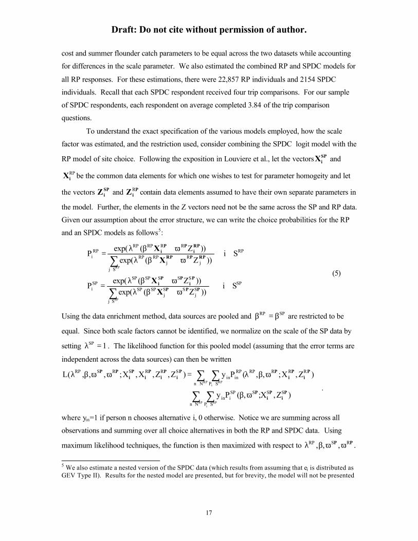
cost and summer flounder catch parameters to be equal across the two datasets while accounting

for differences in the scale parameter. We also estimated the combined RP and SPDC models for

all RP responses. For these estimations, there were 22,857 RP individuals and 2154 SPDC

individuals. Recall that each SPDC respondent received four trip comparisons. For our sample

of SPDC respondents, each respondent on average completed 3.84 of the trip comparison

questions.

To understand the exact specification of the various models employed, how the scale

factor was estimated, and the restriction used, consider combining the SPDC logit model with the

RP model of site choice. Following the exposition in Louviere et al., let the vectors SPiX and

RPiX be the common data elements for which one wishes to test for parameter homogeity and let

the vectors SPiZ and P

iZR contain data elements assumed to have their own separate parameters in

the model. Further, the elements in the Z vectors need not be the same across the SP and RP data.

Given our assumption about the error structure, we can write the choice probabilities for the RP

and an SPDC models as follows5:

SP

Sj

Sj

SSj

SPSP

SSSSPSPSPi

RP

Sjj

Rj

RPRP

RRRPRPRP

i

S i ))Z(exp(

))Z(exp(P

S i ))Z(exp(

))Z(exp(P

SP

RP

∈∀ω+βλ

ω+βλ=

∈∀ω+βλ

ω+βλ=

∑

∑

∈

∈

PPP

Pi

PPi

RPPRP

RPi

PPi

XX

XX

(5)

Using the data enrichment method, data sources are pooled and SPRP β=β are restricted to be

equal. Since both scale factors cannot be identified, we normalize on the scale of the SP data by

setting 1SP =λ . The likelihood function for this pooled model (assuming that the error terms are

independent across the data sources) can then be written

)Z,X;,(Py

)Z,X;,,(Py)Z,Z,X,X;,,,(L

SS

Nn SP

SSPiin

RRRRP

Nn SP

RPinin

SRRSRSRP

SP SPi

RP RPi

Pi

Pi

P

Pi

Pi

PPi

Pi

Pi

Pi

PP

∑ ∑

∑ ∑

∈ ∈

∈ ∈

ωβ

+ωβλ=ωωβλ

.

where yin=1 if person n chooses alternative i, 0 otherwise. Notice we are summing across all

observations and summing over all choice alternatives in both the RP and SPDC data. Using

maximum likelihood techniques, the function is then maximized with respect to .,,, RSRP PP ωωβλ

5 We also estimate a nested version of the SPDC data (which results from assuming that ei is distributed as GEV Type II). Results for the nested model are presented, but for brevity, the model will not be presented


18

With the likelihood function estimated, hypothesis testing for parameter homogeneity

was performed. This process is described in detail in Louviere et al. Let the log likelihood

function value for the restricted model, where SPRP β=β is imposed, be denoted by LJoint. Let LSP

and LRP be the log likelihood values for the SPDC and RP models estimated independently. To

test for parameter homogeneity, calculate the test statistic, -2[LSP+LRP-LJoint] distributed as

2),1n( α−χ , where n is the number of restrictions in the model and a is the level of significance

desired. For parameter homogeneity to be accepted the calculated test statistic must be smaller

than the critical value. This specification allows the recovery of the relative scale parameter

between the two data sources. As we have specified the model, any estimate of the scale factor

greater than one implies that the variation of the RP data is greater than the SP data.

Welfare estimation for potential policy changes using the data enrichment methods

described above requires careful thought about how the RP and SPDC models fit together. Since

welfare measurement compares a change in the state of the world (usually as a result of a policy

change) to a baseline condition, the characterization of the baseline is important. To calculate

baseline conditions to be useful in tandem with parameters of the SPDC format, requires

variables to be site specific. The revealed preference data was used to calculate the baseline

conditions for all variables, RPRP Z,X . The baseline management information, while providing

little variation for estimation purposes was useful for establishing baseline conditions (See Table

1). Although this information provided no variation capable of estimating behavioral parameters

using RP data, they were quite useful for establishing baselines for each site. Therefore, the

complete array of site-specific RP information was necessary for the calculation of welfare

estimates as a result of policy changes. Welfare changes were estimation by altering a set of

management measures (bag and size limits or seasonal closures) relative to baseline levels.

To give the reader a better understanding of the mechanics of welfare measurement and

the data enrichment process undertaken here, consider the model presented in equation (5). To

motivate the issues of data enrichment in the context of welfare measurement, assume that all

parameters, including those of interest to fisheries management are identifiable from the RP data.

Following Hanemann, the welfare change (compensating variation) of moving from condition 0,RP

i0,RP

i ,ZX to condition 1,RPi

1,RPi ,ZX can be written as

in the text. For choice structure issues in recreational demand modeling, see Kling and Thompson, Haab and Hicks, Hauber and Parsons, and Jones and Lupi.


19

tcost_rp_b*1

) ))Z(exp(ln() ))Z(exp(ln(W

RPRP Sj

0,j

R0,j

RPRP

Sj

1,j

R1,j

RPRP

−

ω+βλ−ω+βλ=

∑∑∈∈

RPPRPRPPRP XX (6)

Of course, the factors important for management cannot be recovered using RP estimation.

Given this limitation, there are two ways of incorporating the SPDC information. First, we could

calculate the baseline as described above and simply replace the RP parameters with those

estimated from the SPDC model to obtain the equation

tcost_sp_b*1


RPRP Sj

0,j

S0,j

SPSP

Sj

1,j

S1,j

SPSP

−

ω+βλ−ω+βλ=

∑∑∈∈

RPPRPRPPRP XX (7)

The problem with this approach is that it ignores the effect of the scale parameter. Even if the

underlying behavioral responses are equal ( PP RSRPSP , ω=ωβ=β ), the estimate of compensating

variation and choice probabilities could be quite different because of a failure to account for the

scale factor.

If jointly estimated with restrictions in place, the appropriate welfare measure is

tcost_b*1


RPRP Sj

0,j

S0,j

RP

Sj

1,j

S1,j

RP

−

ω+βλ−ω+βλ=

∑∑∈∈

RPPRPRPPRP XX (8)

where the scale factor is recovered from the RP data and the constraint RPSP β=β is imposed. We

estimate welfare changes using both equation (7) and (8) for each the SPDC models.

Additionally, predictions of participation changes are recovered using estimated choice

probabilities. When management measures are tightened, the probability of choosing the ‘Don’t

Go’ option increases since it is relatively more attractive. We predict someone as ‘Not

Participating’ when the estimated probability of ‘Don’t Go’ is greater than all other estimated

choice probabilities in the model.

V. Results

The discussion above refers to a large number of models to be estimated ranging from

stand-alone RP and SPDC models to jointly estimated ones. We also vary the sample sizes for

many of the jointly estimated models to include only those observations for which RP and SPDC

observations exist to models that include the full sample of RP observations. The goal of this

extensive empirical analysis is to investigate the conditions under which preference homogeneity

can be shown to exist and to provide information about future work involving SPDC modeling.

Important policy relevant questions will hopefully be answered such as the consistency of results

SPDC and RP, the implications for welfare analysis if parameter homogeneity is rejected, and the


20

appropriate choice structure for the SPDC models. Table 6, describes in detail all of the

estimated models. For each of the models listed above, we will investigate differences in welfare,

changes in participation, and parameter estimates in order to answer some of these questions.

Table 6. Estimated Models

Model Description Sample

I. SPDC Discrete choice model of site and participation choice based upon SPDC experimental design.

N=2154 SPDC respondents

II. Nested SPDC Nested discrete choice of participation and then site choice based upon SPDC experimental design.


III. RP (SPDC Sample) Discrete choice model of site choice. Based upon observable choices of Mid-Atlantic recreational angling.


IV. RP (All RP Sample) Discrete choice model of site choice. Based upon observable choices of Mid-Atlantic recreational angling.

N=22857 RP respondents

V. RP/SPDC (SPDC Sample) Jointly estimated RP and SPDC site/participation models


VI. RP/Nested SPDC (SPDC Sample) Jointly estimated RP and SPDC site/participation models. The SPDC model is nested at the participation decision level.


VII. RP/SPDC (All RP Sample) Jointly estimated RP and SPDC site/participation models

N=2154 SPDC respondents, 22857 RP respondents

VIII. RP/Nested SPDC (All RP Sample) Jointly estimated RP and SPDC site/participation models. The SPDC model is nested at the participation decision level.

N=2154 SPDC respondents, 22857 RP respondents

To start, four models were separately estimated. First, we constructed the data necessary

to estimate the RP choice structure. To do this, we calculated travel cost and expected catch rates

(for both summer flounder and all-other fish species) for counties from Massachusetts to Virginia.

Summer flounder recreational angling occurs further south than Virginia, but our data was limited

in its southern extreme because of regional designations in data collection techniques. However,

it is felt that the region examined in this study captures the primary area of summer flounder

fishing and therefore the preferences of anglers potentially impacted by policy.

The RP models, are presented in Table 7 (denoted by models III and IV). Model III

contains the results of the site choice model for those respondents who were observed in both the


21

RP and SPDC data sources. This effectively ‘throws out’ some RP data that could be useful in

identifying behavioral parameters for anglers’ site choices. However, it does allow for the more

restrictive test of parameter homogeneity- where parameter estimates are compared across the

same respondents. The travel cost and other catch coefficient is significant at the 5% level, but

the parameter on summer flounder catch is not significant. Other studies have shown that

identifying species-specific parameters is difficult at best and can be even more problematic if

less than the full dataset is used for estimation. The complete RP data set is used in the

estimation of model IV. In this model, all parameters are significant at the 5% level. For both of

the RP models, anglers are more likely to visit closer sites, or those with higher levels of summer

flounder or ‘other catch’ if the other factors are held constant.

Models I and II in Table 7 provide the estimation results for the SPDC models, both

nested and non-nested (recall the alternative choice structures depicted in Figure 3). For each

respondent the data provided information on the version of the survey administered, so that the

appropriate experimental design could be matched to responses. For the ‘Don’t Go’ option, we

specified a dummy variable to capture any unobservable effects particular to the participation

decision in the model. This was done for the nested and non-nested version of the model. The

nested model was included in order to relax the IIA restriction, which was discussed previously.

All parameters in both models are significant at the 5% level. The estimate on the level of

similarity across the participation decision, b_sp_iv, is greater than one (a required condition for a

well behaved utility function) 6. We tested the restriction that b_sp_iv=1 (which would result in

the standard non-nested model) and found that the nested model was indeed the preferred model

at the 5% level of significance.

Similar results, found in Table 8, were obtained from jointly estimated models using the

sample of respondents in the SPDC models (Models V and VI). These models were obtained by

jointly estimating the RP and SPDC models while placing restrictions on the travel cost and

summer flounder catch coefficients. All parameters are significant at the 5% level. Again, the

nested model is preferred to the non-nested model at the 5% level of significance. Using the full

sample of RP data (which effectively brings the most information to the model), Models VII and

VIII were obtained by jointly estimating the RP and SPDC models, with the same restrictions as

those found in Models V and VI. The results are quite similar than other jointly estimated

6 Following Morey’s notation, b_sp_iv=σ−1

1, where 1-s is termed the inclusive value parameter in

McFadden.


22

models. This time, the nested model is preferred to the non-nested model at the 10% level of

significance.

Table 7. RP and SPDC estimation results (t statistics in parenthesis)*.

I II III IV Parameter SP Nested SP RP (SPDC

sample) RP (All RP sample)

b_sp_tcost -.0140 (-14.10)

-.0118 (-8.74)

b_sp_sf .0601 (12.95)

.0515 (8.82)

b_sp_bag .0708 (15.47)

.0606 (9.48)

b_sp_sznum .0080 (19.25)

.0068 (9.73)

b_sp_oca .2358 (5.18)

.2040 (4.88)

b_sp_ocb -.4186 (-9.91)

-.3558 (-7.554)

b_sp_home -.8168 (-11.53)

-1.0352 (-8.30)

b_sp_iv 1.2079 (10.17)

b_rp_tcost -.0271

(-20.85) -.0240

(-60.73) b_rp_sf .0331

(1.13) .0728 (7.07)

b_rp_oc .0515 (4.44)

.0595 (16.31)

?RP χ2(all parms=0) 4095.52 4099.71 534.17 4577.03 N (people) 2154 2154 2154 22857 N (discrete choices) 8279 8279 2154 22857

*All estimates were obtained using full information maximum likelihood estimators written in

Gauss v. 3.5 and the Gauss Constrained Maximum Likelihood Module v 1.


23

Table 8. Joint Estimation of RP and SPDC Models (t statistics in parenthesis)*.

Subset of obs where sp and rp data exists, n=2154

All obs, SP n=2154; RP n=22857

V VI VII VIII Parameter RP/SP RP/Nested SP RP/SP RP/Nested SP

b_sp_tcost -.0145 (-16.11)

-.0124 (-8.86)

-.0147 (-16.33)

-.0126 (-9.69)

b_sp_sf .0570 (12.67)

.0491 (8.77)

.0553 (13.17)

.0477 (8.83)

b_sp_bag .0707 (15.37)

.0608 (9.50)

.0707 (15.37)

.0609 (9.52)

b_sp_sznum .0082 (20.50)

.0070 (10.01)

.0083 (20.75)

.0071 (10.14)

b_sp_oca .2345 (5.15)

.2039 (4.85)

.2338 (5.14)

.2038 (4.84)

b_sp_ocb -.4229 (-10.09)

-.3615 (-7.63)

-.4250 (-10.17)

-.3646 (-7.69)

b_sp_home -.8558 (-12.46)

-1.0623 (-8.74)

-.8759 (-13.48)

-1.0772 (-9.03)

b_sp_iv 1.2005 (10.23)

1.1964 (10.25)

b_rp_tcost -.0145

(-16.11) -.0124 (-8.86)

-.0147 (-16.33)

-.0126 (-9.69)

b_rp_sf .0570 (12.67)

.0491 (8.77)

.0553 (13.17)

.0477 (8.83)

b_rp_oc .0245 (3.71)

.0208 (3.47)

.0362 (10.97)

.0310 (7.95)

?RP 1.8307 (12.62)

2.1480 (8.44)

1.6202 (15.81)

1.8935 (9.27)

χ2(all parms=0)

4622.22 4626.17 8667.80 8671.67

N (people) SP=RP=2154 SP=RP=2154 SP=2154 RP=22857

SP=2154 RP=22857

N (discrete

choices)

SP=8279

RP=2154

SP=8279

RP=2154

SP=8279

RP=22857

SP=8279

RP=22857

Restrictions b_sp_tcost=

b_rp_tcost

b_sp_sfcatch=

b_rp_sfcatch

b_sp_tcost=

b_rp_tcost

b_sp_sfcatch=

b_rp_sfcatch

b_sp_tcost=b_rp_tcost

b_sp_sfcatch=

b_rp_sfcatch

b_sp_tcost=b_rp_tcost

b_sp_sfcatch=

b_rp_sfcatch

*All estimates were obtained using full information maximum likelihood estimators written in

Gauss v. 3.5 and the Gauss Constrained Maximum Likelihood Module v 1.


24

There are significant similarities across the jointly estimated models. All signs are as expected.

Anglers tend to prefer closer sites, those with higher levels of catch, and those with less restrictive

levels of management (higher bag limits and lower minimum size restrictions). The choice

specific dummy on the ‘don’t go’ option, is always negative, indicating that all things equal, the

angler is more likely to choose to participate than not. The marginal value coefficients, found by

dividing a coefficient with the absolute value of the travel cost coefficient are also quite similar

across the models. Summer flounder catch (in the range of $4.76 to $4.36), bag limits (in the

range of $4.80 to $5.14), and size limits interacted with expected number of legal size (in the

range of $0.56 to $0.58) are all quite close to one another. The only discernible pattern when

comparing the models is that the stand-alone SPDC models (Models V and VI), that imposed no

restriction on the parameters, tended to lead to higher marginal value estimates. We also

compared the marginal value estimates of summer flounder catch to the RP models to all of the

other models (Table 9). Findings show that the RP estimates of the marginal value of summer

flounder catch is lower than any found using the SPDC data.

For the restricted models in Table 10, the scale factor (?RP) is always greater than one and

the estimated magnitudes (in the range of 1.62 to 2.15) indicate that the variance of the RP data is

on average nearly three times that found in the SP data. Tests for homogeneity of parameters

across the different models, while accounting for this difference in the scale factor, were

performed. Using Models V-VIII, tests were performed for each model to examine if the more

restrictive model (where the scale factor is estimated and restrictions are placed across the RP and

SPDC models) is preferred to separate estimation of the models. All tests for preference

homogeneity (for the travel cost and summer flounder catch parameters) failed at the 10%

significance level using the statistical test described above. The implications for these findings

for policy are two-fold:

(1) While all signs for parameters across the RP and SP models agree in sign, there is

small but statistically significant divergence in their actual magnitude.

(2) Despite the findings that parameter estimates are not homogenous across data

sources, the RP estimation provides no way to estimate management-specific

behavioral parameters.

The challenge is to reconcile these seemingly contradictory items in a reasonable way.

Since the goal of this research is to provide a tool that will provide fishery-specific, policy-

relevant input, we next examine differences in the predictions of welfare participation changes

across the different models. To accomplish this, we begin by examining the differences between

predicted welfare change in the RP and all SPDC models due to a change in environmental


25

conditions in summer flounder catch. These results offer evidence that the two models estimated

independently of each other and from separate data sources provide similar albeit statistically

different policy guidance with regard to changing management conditions. If these results were

found to be different in orders of magnitude, then less faith could be placed on the SPDC data and

how preferences estimated from such data might reflect real-world choices. Results are presented

in Table 11 for two policies that increase summer flounder catch by 25% and 50%. The results

show that estimates across all of the models, despite rejecting the hypothesis of preference

homogeneity, are remarkably close even when comparing the RP models with the other models in

the paper. Ninety-five percent confidence intervals were constructed using the Krinsky-Robb

technique with 1000 draws of the parameter vector. There is some overlap in the confidence

intervals depending on the actual model compared. The mean CV for the full RP model (whose

welfare estimates are statistically different from zero) is very close to residing inside the 95%

confidence intervals for every other model estimated. Comparing results across all of the SPDC

models show that regardless of the definition of sample sizes or nesting structure, that welfare

estimates are not different from each other. There are a few comparisons that are statistically

different, but overall all models are virtually identical to one another.

Table 9. Measures of Compensating Variation for a change in environmental quality*,**.

*Confidence intervals computed using the Krinsky-Robb method with 1000 draws.

**The number of legal sized fish is not allowed to change in this measure.

RP Models SPDC Models Data Enrichment Models

Subset of RP Obs

Data Enrichment Models

All RP Obs

III IV II I VI V VIII VII

Quality Change Subset of

RP Obs.

All RP Obs. Nested Non-nested Nested Non-nested Nested Non-nested

Marginal Value of s.

flounder catch

1.22 3.03 4.36 4.29 3.95 3.93 3.78 3.76

+25% ? in s. flounder

catch

$0.83

(-.82,2.20)

$1.90

(1.14,2.49)

2.60

(1.97,3.04)

2.52

(1.94,3.08)

2.74

(2.42,2.98)

2.58

(2.26,2.86)

2.52

(2.26,2.71)

2.29

(2.04,2.51)

+50% ? in s. flounder

catch

1.69

(-1.64,4.48)

3.85

(2.30,5.06)

5.25

(3.99,6.16)

5.09

(3.92,6.23)

5.61

(4.94,6.11)

5.26

(4.60,5.84)

5.14

(4.60,5.53)

4.65

(4.15,5.11)

To further examine how each of the six SPDC models perform, we examine participation

and welfare measures for potential policy changes that fisheries managers might want to consider.

We alter the bag and minimum size limits relative to baseline levels in Table 10. The first row of

the table is associated with more restrictive policies that are loosened as one moves down the

rows in the table. Findings show that anglers are willing to pay more to avoid more restrictive

bag limits than size limits. However, anglers are willing to pay significant amounts to avoid

either type of policy. Examining the relative performance across models, show strikingly similar

results across models. Again, nearly without exception, mean measures of CV fall within the

95% confidence intervals of the other potential SPDC models. This provides some evidence that

the choice of sample or choice-structure does not impact policy-relevant model outputs in

appreciable ways.

Changes in participation (defined here as trips) estimates for the same policies are

reported in Table 11. These estimates were computed by comparing the predicted number of

respondents who would not have participated before and after the policy change. We then use

predicted non-participants to estimate the percent of the sample who would not have participated

due to the policy change. This percentage is then multiplied by the estimated number of trips in

the Mid-Atlantic region in 2000 (MRFFS personal correspondence) to arrive at predicted

participation changes. While confidence intervals are not reported, the reader should note they

are available from the author. None of the reported participation changes were significantly

different from zero.


28

Table 10. Measures of CV for some selected policy changes (95 % confidence intervals in

parenthesis*).

Policy Change

SPDC Models Data Enrichment Models Subset of RP Obs

Data Enrichment Models All RP Obs

II I VI V VIII VII Bag Size Nested Non-nested Nested Non-nested Nested Non-nested -3 3 -$17.43

(-22.77,-14.84) -$17.13

(-20.06,-14.87)

-$17.47 (-19.30,-16.38)

-$17.15 (-18.59,-15.96)

-$17.11 (-18.98,-15.95)

-$16.82 (-16.95,-18.36)

-3 0 -13.87 (-18.69,-11.66)

-13.68 (-16.09,-11.57)

-13.53 (-15.08,-12.58)

-13.40 (-14.58,-12.30)

-13.29 (-14.92,-12.28)

-13.18 (-14.47,-12.00)

-1 1 -6.55 (-8.44,-5.59)

-6.42 (-7.51,-5.62)

-6.66 (-7.34,-6.25)

-6.51 (-7.05,-6.08)

-6.51 (-7.19,-6.08)

-6.37 (-6.95,-5.91)

1 -1 7.54 (6.25,8.63)

7.38 (5.90,8.40)

7.85 (7.25,8.35)

7.61 (6.79,8.15)

7.64 (7.02,8.16)

7.43 (6.55,7.99)

0 -3 10.55 (8.72,12.22)

10.17 (8.63,11.73)

12.52 (11.31,13.53)

11.67 (10.70,12.59)

11.97 (10.77,12.91)

11.18 (10.15,12.15)

3 -3 24.65 (20.59,28.23)

24.08 (19.38,27.42)

26.29 (24.24,28.05)

25.32 (22.68,27.11)

25.50 (23.40,27.31)

24.60 (21.78,26.50)

*Confidence intervals computed using the Krinsky-Robb method with 1000 draws.

Table 11. Measures of changes in trips for some selected policies*.

Policy Change

SPDC Models Data Enrichment Models Subset of RP Obs

Data Enrichment Models All RP Obs

II I VI V VIII VII Bag Size Nested Non-nested Nested Non-nested Nested Non-nested

-3 3 0 -69,436 -1877 -75,067 -1877 -75,067 -3 0 0 -37,533 -1877 -60,053 -1877 -69,437 -1 1 0 -18,766 0 -20,643 0 -22,520 1 -1 0 13,700 0 16,890 0 16,890 0 -3 0 6,558 0 5,630 0 7,507 3 -3 0 26,273 0 30,027 0 31,903


29

These estimates show that the choice of model structure and sample can lead to different

estimates of participation changes. Because not very many respondents in the SPDC survey

indicated they would choose the ‘don’t go’ option, very large swings in participation only happen

in association with large policy changes. The most striking results in Table 11 are the relative

performance between the nested and non-nested model. Despite adding a first level nest for the

participation choice, the nested model predicts almost no participation effects from any of the

policy changes. In this regard, the non-nested models are more responsive. The nested model

largely reallocates changes in behavior within the site choice level of the model because the

nesting structure makes it more costly to substitute away from fishing toward some other activity.

Therefore, paradoxically, the non-nested model provides a more responsive participation model.

We have also computed participation and welfare changes for quite a number of potential

policies to develop a response surface based upon CV. Assuming that policies with higher CV

are preferred to policies with lower CV, we found that all models predict the same ordering of

policy alternatives from most preferred to least preferred. Coupling this with the finding that the

RP and the SPDC models predict levels of CV very close to one another (from Table 9) provides

evidence that the SPDC enrichment models are a defensible way of incorporating respondents

preferences despite the rejection of preference homogeneity across the RP and SPDC models.

VI. Conclusion

This paper presents a methodology for quantifying people’s preferences for

environmental conditions or management that are not readily identifiable using real-world

observations. For many reasons, including lack of variation or the exploration of a new

management technique, RP methods may not provide adequate information in a large number of

settings for environmental managers. The SPDC presented here provides a rigorous way of

getting at important attributes like this. The experimental design technique, used for constructing

hypothetical comparisons of trips, is a very powerful and efficient way of data collection coupled

with minimal burden on respondents.

Additionally, we have shown that the existing data revealed preference data collection

programs can be used to readily collect data necessary for the implementation of stated preference

techniques. The field intercept survey is an extremely effective way gaining information about

the real choices that people make regarding recreational angling. Combining the intercept survey

with a mail data collection methodology for the collection of the SPDC survey proved to be an

effective way of combining these data sources.


30

Models were estimated using both revealed and stated preference data. Where data

existed for common elements in the revealed and stated preference data, we estimated restricted

models to test for parameter homogeneity across RP and SPDC models. For every model

estimated, we rejected the hypothesis of partial preference homogeneity across the data sources.

Even in the presence of these findings, the question remained of how to quantify angler’s

preferences for management when there was no way to recover these behavioral parameters from

revealed preference data.

Despite the findings of partial preference heterogeneity across the RP and SPDC data

sources, the results also show that while statistically different, nearly without exception the

models predict welfare changes on par with each other. As for model structure and the choice of

sample, the SPDC models all predict quite similar welfare changes for every policy examined.

Perhaps the only discernible difference between alternative model structures was in the prediction

of participation changes. These results showed that the non-nested model provided the most

responsive prediction model. However, predicted participation changes were very small relative

to the overall activity in the mid-Atlantic region and not statistically different from zero.

The results also show that this technique is potentially very useful for a whole host of other

management problems such as marine protected areas, marine mammal protection, turtle

protection, and developing performance metrics for ecosystem management. Because the

technique does not necessarily require a large body of baseline data, it can be used to quickly

assess people’s preferences for environmental resources and management.


31

References

Adamowicz, W., J. Louviere, and M. Williams. (1994). “Combining Revealed and Stated

Preference Methods for Valuing Environmental Amenities.” Journal of Environmental

Economics and Management, 26: 271-92.

Adamowicz, W., J. Swait, P. Boxall, J. Louviere, and M. Williams. 1997. “Perceptions versus

objective measures of environmental quality in combined revealed and stated preference

models of environmental valuation.” Journal of Environmental Economics and

Management, 32: 65-84.

Ben-Akiva, M. E. and T. Morikawa. (1990). “Estimating switching models from revealed

preferences and stated intentions’, Transportation Research A 24A(6):485-95.

Bockstael, N., K. McConnell, and I. Strand. 1989. “A Random Utility Model for Sportfishing:

Some Preliminary Results for Florida.” Marine Resource Economics v6.

Bockstael, N. E., K. McConnell, and I. Strand. 1991. “Recreation.” In Braden, J. and C. Kolstad,

P. (ed.), Measuring the Demand for Environmental Quality. Elselvier Science

Publishers B. V.

Dillman, D. 1978. Mail and telephone surveys: The total design method. Wiley Publishers:

New York.

Green, G., C. Moss, and T. Spreen. 1997. “Demand for Recreational Fishing Trips in Tampa

Bay Florida: a Random Utility Approach.” Marine Resource Economics , v12(4).

Guadagni, P. M. and J. D. Little. 1983. “A logit model of brand choice calibrated on scanner

data.” Marketing Science 2(3):203-38.

Haab, T. and R. Hicks. “Choice Set Considerations in Models of Recreation Demand.” Marine

Resource Economics , v14(4).

Hanemann, W. M., “Applied Welfare Analysis with Qualitative Response Models”. Working

Paper No. 241. Department of Agricultural and Resource Economics. University of

California at Berkeley (1982).

Hauber, A. B. and G. Parsons. 2000. “The Effect of Nesting Structure Specification on Welfare

Estimation in a Random Utility Model of Recreation Demand: an Application to the

Demand for Recreational Fishing.” American Journal of Agricultural Economics , v.

82(3).

Herrmann, Mark, S. Todd Lee, Charles Hamel, Keith R. Criddle, Hans T. Geier, Joshua A.

Greenberg and Carol E. Lewis. “An Economic Assessment of the Sport Fisheries for

Halibut, Chinook and Coho Salmon in Lower Cook Inlet.” Final Report to the Mineral

Management Service, Coastal Marine Institute, OCS Study MMS 2000-061, April 2001.


32

Hicks, R. Volume II: The Economic Value of New England and Mid-Atlantic Sportfishing

in 1994. NOAA Technical Memorandum NMFS-F/SPO-38. August 1999.

Jones, C. and F. Lupi. 1999. “The Effect of Modeling Substitute Activities on Recreation

Benefit Estimates.” Marine Resource Economics v14(4).

Kaoru, Y. 1995. “Measuring Marine Recreation Benefits of Water Quality Improvements by the

Nested Random Utility Model.” Resource and Energy Economics v17(2), pp. 119-36.

Kaoru, Y. and V. Smith. 1995. Using random utility models to estimate the recreational value of

estuarine resources. American Journal of Agricultural Economics Feb 1995 v77 n1

p141(11)

Kling, C. and C. Thomson. “Implications of Model Structure for Welfare Estimation in Nested

Logit Models.” American Journal of Agricultural Economics v. 78(1).

Krinsky, I., and L. Robb. 1990. “On approximating the statistical properties of elasticities: a

correction.” The Review of Economics and Statistics v. 72(1) pp.189-90.

Lancaster. K. (1966). “A new approach to consumer theory”, Journal of Political Economy v.

74, pp. 132-157.

Lancaster, K. (1971). Consumer demand: a new approach, New York: Columbia University

Press.

Layton, D. (2001). “Alternative approaches for Modeling Concave Willingness to Pay Functions

in Conjoint Valuation.” American Journal of Agricultural Economics v. 83(5).

Louviere, J., D. Hensher, and J. Swait. 2000. Stated Choice Methods: Analysis and

Application. Cambridge University Press.

McConnell, K. and I. Strand. 1994. Volume II: The Economic Value of Mid and South

Atlantic Sportfishing. Report on Cooperative Agreement #CR-811043-01-0 between

the University of Maryland, U.S. Environmental Protection Agency, National Oceanic

and Atmospheric Administration, and the National Marine Fisheries Service.

McConnell, K., E., I. Strand, and L. Blake-Hedges. 1995. “Random Utility Models of

Recreational Fishing: Catching Fish Using a Poisson Process”. Marine Resource

Economics, v10(3), pp. 247-261.

McFadden, D. (1974). “Conditional logit analysis of qualitative choice behavior.” In

Zarempbka, P. (ed.), Frontiers in econometrics , New York: Academic Press, pp. 105-

42.

Mitchell, R. C. and R. T. Carson. 1989. Using surveys to value public goods: the contingent

valuation method. Baltimore, MD. Johns Hopkins University Press for Resources for

the Future.


33

Parsons, G. and M. Needelman. 1992. “Site Aggregation in a Random Utility Model of

Recreation.” Land Economics v68(4).

Parsons, G., A. Plantiga, and K. Boyle. 2000. “Narrow Choice Sets in Random Utility Models of

Recreation Demand.” Land Economics v76(1).

Parsons, G. and A. B. Hauber. 1998. “Spatial Boundaries and Choice Set Definition in a

Random Utility Model of Recreation Demand.” Land Economics v74(1).

Pendleton, L. and R. Mendelsohn. Estimating the economic impact of climate change on the

freshwater sportsfisheries of the northeastern U.S. Land Economics Nov 1998 v74 i4

p483(1).

Preston, J. 1991. “Demand Forecasting for New Local Rail Stations and Services.” Journal of

Transport Economics and Policy, V.25(2) pp. 183-202.

Schuhmann, P. 1998. “Deriving Species-Specific Benefit Measures for Expected Catch

Improvements in a Random Utility Framework.” Marine Resource Economics v13(1).

Swait, J. J. Louviere, and M. Williams. (1994). “A sequential approach to exploiting the

combined strengths of SP and RP data: application to freight shipper choice.”

Transportation 21:135-52.

Swait, J. and W. Adamowicz. 1996. “The effect of choice environment and task demands on

consumer behavior: discriminating between contribution and confusion.” Department of

Rural Economy, Staff paper 96-09, University of Alberta. Alberta, Canada.

Documents

A Comparison of Stated and Revealed Preference Methods for