Embed Size (px)
Citation preview
A Computational and Experimental Study of
Viscous Flow Around Cavitating Propulsors
by
Wesley H. Brewer
B.S., University of Tennessee (1993)
Submitted to the Department of Ocean Engineeringin partial fulfillment of the requirements for the degree of
Master of Science in Ocean Engineering
at the
MASSACHUSETTS INSTITUTE OF TECHNOLOGY
June 1995
@ Massachusetts Institute of Technology 1995
Signature of Author ................. 4V j, 'r ..
Department of Ocean EngineeringMay 1995
OF TECHNOLOGY
DEC 0 8 1995
LIBRARIES
Certified by ........ ... .. e....
ecturer
Accepted by....
Dr. Spyros A. Kinnasand Principal Research Engineer
Thesis Supervisor
Professor . Doug as CarmichaelChairman, Departmental Committee on Graduate Students
A Computational and Experimental Study of Viscous Flow
Around Cavitating Propulsors
by
Wesley H. Brewer
Submitted to the Department of Ocean Engineeringon May 1995, in partial fulfillment of the
requirements for the degree ofMaster of Science in Ocean Engineering
Abstract
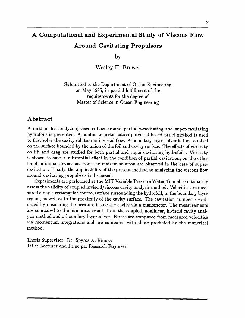
A method for analyzing viscous flow around partially-cavitating and super-cavitatinghydrofoils is presented. A nonlinear perturbation potential-based panel method is usedto first solve the cavity solution in inviscid flow. A boundary layer solver is then appliedon the surface bounded by the union of the foil and cavity surface. The effects of viscosityon lift and drag are studied for both partial and super-cavitating hydrofoils. Viscosityis shown to have a substantial effect in the condition of partial cavitation; on the otherhand, minimal deviations from the inviscid solution are observed in the case of super-cavitation. Finally, the applicability of the present method to analyzing the viscous flowaround cavitating propulsors is discussed.
Experiments are performed at the MIT Variable Pressure Water Tunnel to ultimatelyassess the validity of coupled inviscid/viscous cavity analysis method. Velocities are mea-sured along a rectangular control surface surrounding the hydrofoil, in the boundary layerregion, as well as in the proximity of the cavity surface. The cavitation number is eval-uated by measuring the pressure inside the cavity via a manometer. The measurementsare compared to the numerical results from the coupled, nonlinear, inviscid cavity anal-ysis method and a boundary layer solver. Forces are computed from measured velocitiesvia momentum integrations and are compared with those predicted by the numericalmethod.
Thesis Supervisor: Dr. Spyros A. KinnasTitle: Lecturer and Principal Research Engineer
Acknowledgements
This thesis represents the work of which many people have contributed; I am very for-
tunate to be working among such a talented group of people. I am gratefully indebted
to Spyros Kinnas for more than generous amounts of encouragement, advice, and assis-
tance. Dr. Kinnas' unselfish motivation to help students has granted me the opportunity
to achieve many goals that otherwise would not have been possible. I would also like
to thank Professor Drela for his assistance in adapting the viscous routines of XFOIL
to cavitating flow. Also, much thanks goes to Professor Justin Kerwin for his excellent
advice in times of need and to all those in the propeller group. I especially would like
to express my appreciation to Shige Mishima, whose talented help in both academics
and research was invaluable to the completion of this work. I am also grateful to my
roommate Jesse Hong, for his expert advice on computers and for putting up with me
over the years. Additional thanks go to our UROP'S Matt Knapp, Dianne Egnor, and
Luke Sosnowski, for helping out in all phases of the experiment.
Most importantly I would like to thank my fiance Jenny, to whom I dedicate this
thesis. Her constant love, devotion, and support has made graduate school much more
fulfilling.
Much support also came from friends and family. A special thanks goes to my mother,
for always believing in me. I could not have made it through college and graduate school
without her substantial financial and emotional support. I also thank my dad for always
inspiring me to the best and showing me a strong work ethic, and Michelle for always
giving encouragement in times of need. Lastly, but most importantly, I would like to
thank God who makes all things possible.
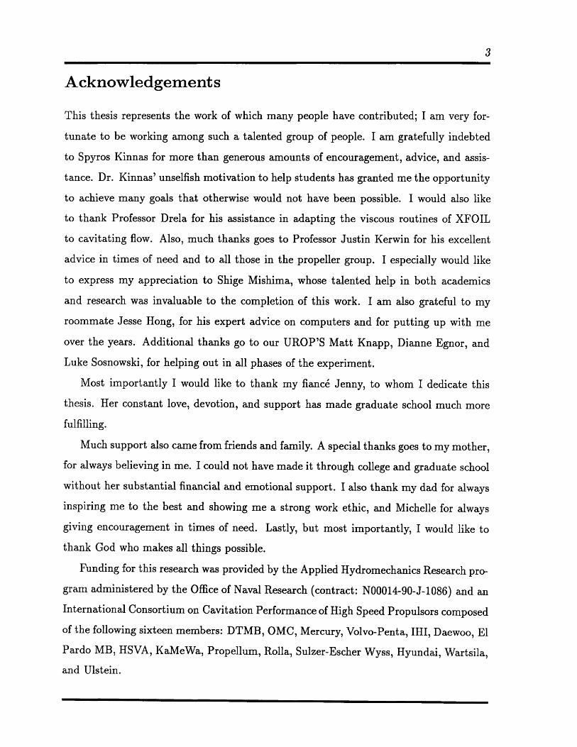
Funding for this research was provided by the Applied Hydromechanics Research pro-
gram administered by the Office of Naval Research (contract: N00014-90-J-1086) and an
International Consortium on Cavitation Performance of High Speed Propulsors composed
of the following sixteen members: DTMB, OMC, Mercury, Volvo-Penta, IHI, Daewoo, El
Pardo MB, HSVA, KaMeWa, Propellum, Rolla, Sulzer-Escher Wyss, Hyundai, Wartsila,and Ulstein.
Contents
1 Introduction 15
1.1 Research History ............................. 16
1.1.1 Experiments .............................. 16
1.1.2 Numerical Methods .......................... 17
1.2 O bjectives . . . . . . . . . . . . . . . . . . . . . . . . . . . . . . .. .. . 19
2 Experiment 21
2.1 Setup . . . . . . . . . . . . . . . . . . . . . . . . . . . . . . . . . .. .. . 22
2.2 Velocity Measurements ............................ 23
2.2.1 Procedure . . . . . . .. . . . . . . . . .. . . . . . . . .. .. . . 23
2.2.2 Errors in Velocity Measurements . ................. 29
2.3 Pressure Measurements ................. ........ . . . . 30
2.4 Geometry of the Foil .... ...... . ..... ........... . 32
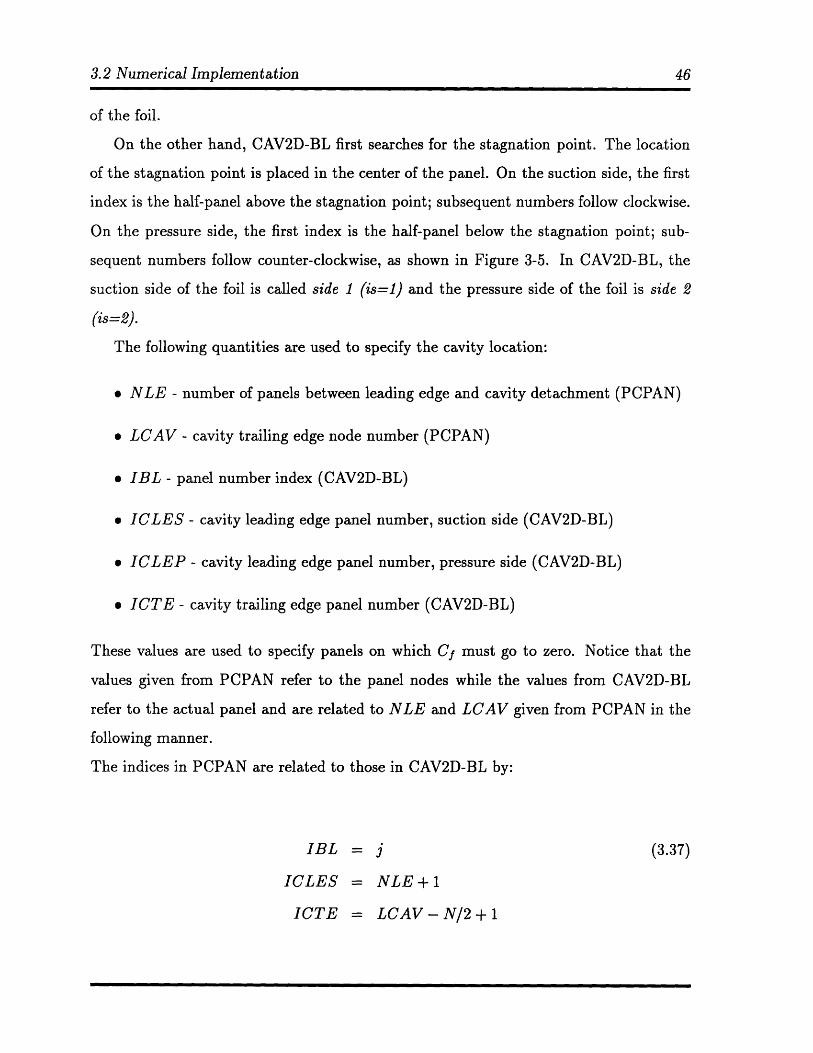
3 CAV2D-BL: Partially-Cavitating Boundary Layer Solver 35
3.1 Form ulation .................................. 35
3.1.1 Inviscid Cavitating Flow Theory . .................. 35
3.1.2 Boundary Layer Theory ....................... 38
3.2 Numerical Implementation .......................... . 39
3.2.1 Step 1: Calculate the cavity height (PCPAN) . .......... 40
3.2.2 Step 2: Calculate inviscid edge velocity on compound foil (CAV2D-
B L ) . . . . . . . . . . . . . . . . . . . . . . . . . . . . . . . . . . 40
CONTENTS
3.2.3 Step 3: bolve the boundary layer equations
(CAV2D-BL) ..................
3.2.4 Step 4: Update the edge velocity (CAV2D-BL)
3.2.5 Indexingofthepanels . . . . . . . . . . . . .
3.3 Analytical Forces ......................
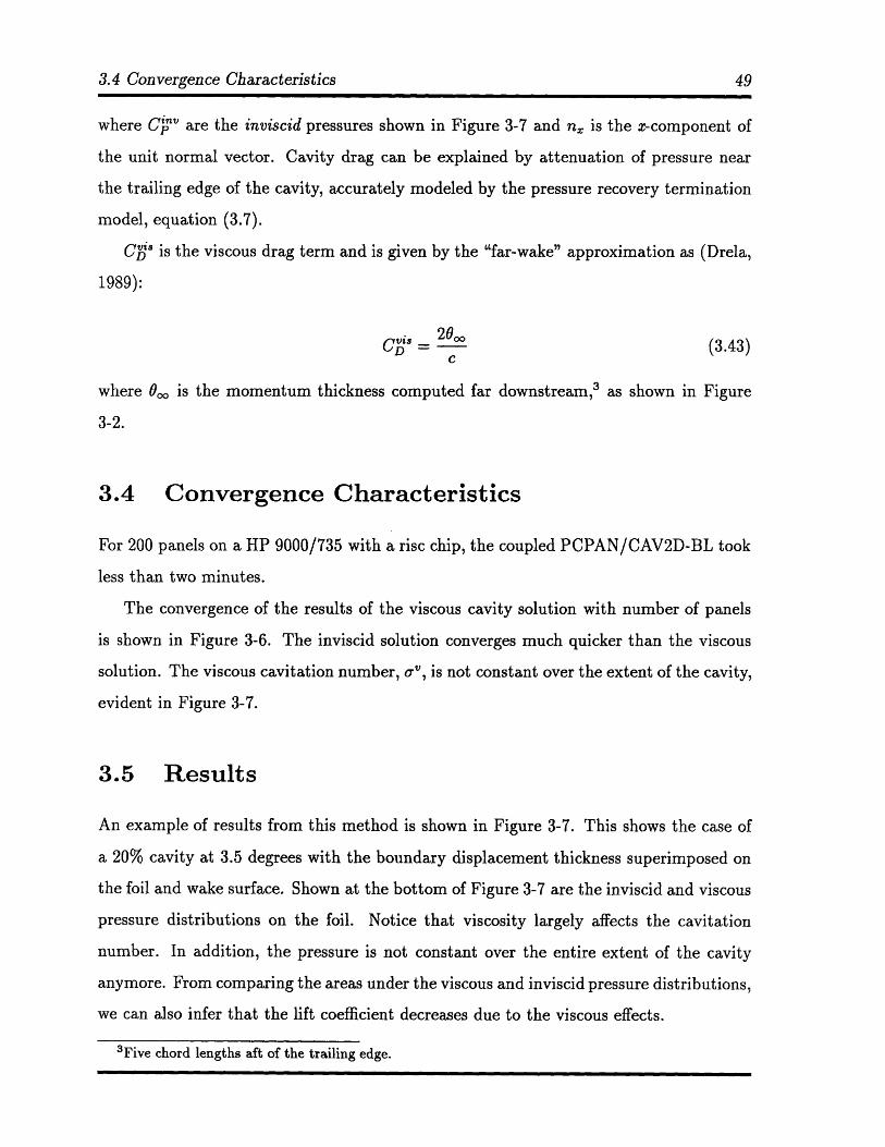
3.4 Convergence Characteristics ................
3.5 R esults . . . . . . . . . . . . . . . . . . . . . . . . . . . .
3.6 Cavity Detachment Point ..................
3.7 Effects of Tunnel Walls ...................
4 CAV2D-BL: Super-Cavitating Boundary Layer Solver
4.1 Formulation & Numerical Implementation . . . . . . . .
4.1.1 Step 1: Calculate cavity height (SCPAN) . . . . .
4.1.2 Steps 2 & 3: Solve viscous flow around "compound"
4.2 Indexing of the panels . . . . . . . . . .
4.3 Results .. . . . . . . . . . . . . .. . . .
5 Experimental Versus Numerical Results:
5.1 Forces in the Experiment .........
5.1.1 Method of Calculation ......
5.1.2 Comparisons with Theory . . . .
5.2 Velocity Comparisons ...........
5.2.1 Near the Cavity Surface . . . . .
5.2.2 On Rectangular Control Surface .
5.2.3 In the Boundary Layer . . . . . .
Phases
rr, r r ·
foil
II & III
. . . . . ,
• . .•
5.2.4 Pressure Measurements . . . . . . . . . .
5.2.5 Errors in Determining the Foil Surface .
(CAV2D-BL)
... .... 59
63
... .... 64
... .... 64
. . . . . . . 65
... .... 66
. . . . . . . 66
. . . . . . . 66
. . . . . . . 70
. . . . . . . 70
. . . . . . . 78
6 Conclusions
6.1 Application to Propulsor Blades.......................
6.2 Recommendations ...............................
compound foil
.........
.. o......
........ a.
.........
........ ,
.,.......
...... o..
CONTENTS
6.3 Preliminary "Momentum Jump" Model . .................. 84
A Calculating Displacement Thickness
B Boundary Layer Construction
C Experimental Data: Phase I
D Experimental Versus Numerical Results: Phase I
90
94
101
Nomenclature
B bias limit
c chord
Cd dissipation coefficient = (1/peU3 ) f r(au/Ir7)drI
CD drag coefficient = D/lpU c
Cf skin-friction coefficient = 27waIi/pu
CL lift coefficient = L/ pUc
Cp pressure coefficient = (P - Poo)/.pUl
CT shear stress coefficient = Tmax/pUe2
C0EQ equilibrium shear stress coefficient
h mercury level in manometer
H shape factor = 6*/0
H" kinetic energy shape parameter = 0*/0
Hk kinematic shape parameter
= f[1 - (U/Ue)]d7 + f(U/Ue)[1 - (u/Ue)]d?7
1 cavity length
n foil surface unit normal vector
Stransition disturbance amplification variable
N number of velocity samples
Pk measured cavity pressure
Pv vapor pressure of water
Poo free-stream pressure
P precision limit = tS
qC cavity surface velocity vector
CONTENTS 8
s arclength along foil surface
S, precision index of the mean = ao/v/-N
t coverage factor
tiax, maximum thickness of foil section
u, w horizontal and vertical velocities
U uncertainty estimate
Ue edge velocity
Uoo free-stream velocity
x stream-wise distance
y vertical distance (analytical)
z vertical distance (experimental)
C angle of attack
6 boundary layer thickness
6:* boundary layer displacement thickness = f(1 - u/Ue)dy
0 boundary layer momentum thickness
= fU/Ue(1 - /Ue)dy
0* kinetic energy thickness = f(u/ue)[1 - u2/u2]dy
PHo2 water density
PiHg mercury density
PLIT leading edge radius of foil
cavitation number = (po - pv)/I~pU
uu standard deviation of horizontal velocity
measurements
blowing source strength
total velocity potential = Din(x, y) + (x, y)
perturbation potential
Din, velocity inflow potential
List of Tables
2.1 Testing cases and setup parameters at a free-stream velocity of 8 m/s (25
ft/s). . . . . . . . . . . .. . . . . . . . . . . . . . .... . . . . . . . .. . 28
2.2 The bias limit, precision limit, and uncertainty estimate of the Flapping
Foil Experiment performed at the MIT Water Tunnel (adjusted from Lurie
(1995)). ................................... .. 302.3 Heavy Foil Coordinates ............................ 34
3.1 Cavitation number and cavity volume from the analysis method, using
both predicted and experimentally observed cavity detachment as input. 52
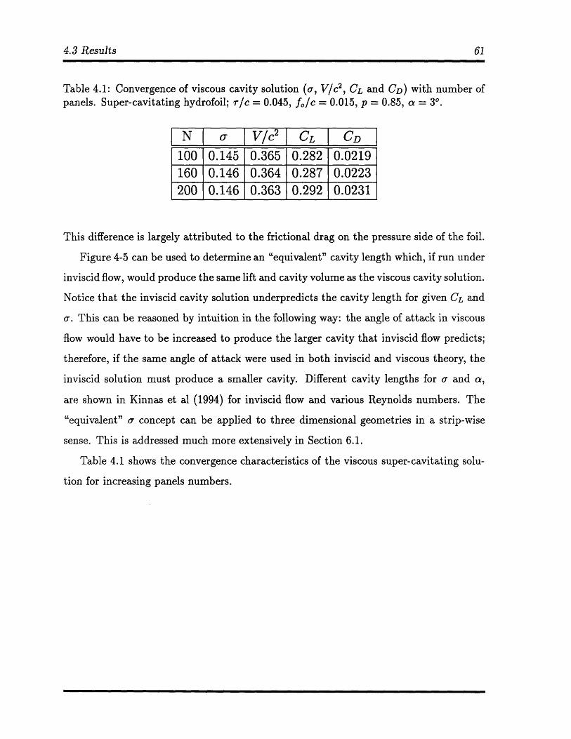
4.1 Convergence of viscous cavity solution (a, V/c 2 , CL and CD) with number
of panels. Super-cavitating hydrofoil; r/c = 0.045, fo/c = 0.015, p = 0.85,
a = 30. . . ..... . . . . . . . . . . . . . . . . . . . . . . . . . . . . . . . 61
5.1 Comparison of lift and drag coefficients between experiment and theory.
a = 3.250 in fully-wetted flow (l/c=0). a = 3.50 in cavitating flow (10%,
20%, 30%, and 40%) .................... .......... 64
5.2 Cavitation number comparisons between experiment and theory, a =
3.250. (exp stands for experimental, p for differential pressure manometer,
ptun for tunnel pressure manometer, vel for velocity measurements, an for
analytical result, inv for inviscid, and vis for viscous.) . .......... 78
List of Figures
1-1 History of code development for two-dimensional cavitating boundary layer
solver. .................................... .. 18
1-2 Hydrofoil with cavity and displacement thickness illustrating where bound-
ary conditions are applied ................... ........ 19
2-1 Experimental setup in water tunnel showing foil and contour path of laser
(all units given in millimeters). ....................... 23
2-2 Photographs of the hydrofoil in the water tunnel testing section. Top:
l/c=0.10, bottom: l/c= 0.20. a = 3.50. ................... 24
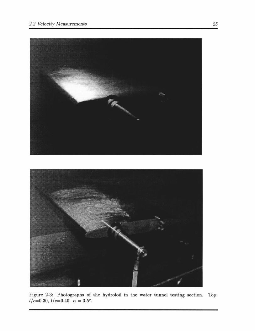
2-3 Photographs of the hydrofoil in the water tunnel testing section. Top:
l/c=0.30, l/c=0.40. a = 3.50. ........................ 25
2-4 Horizontal velocity measurements on the top and bottom of a rectangular
contour surrounding the hydrofoil with error bars showing plus or minus
one-half standard deviation. ......................... 27
2-5 Example of boundary layer cuts near foil surface. a = 3.50 ........ 27
2-6 Top and side view of hydrofoil, in tunnel testing section, showing the
location of the pressure tap. ......................... 31
2-7 Manometer setup in water tunnel. . .............. ... .. . . . . 32
2-8 Plot of foil surface ............................... 33
3-1 Hydrofoil with imposed boundary conditions ................. 36
3-2 Hydrofoil with displaced body. Definition of main parameters. a = 3.50 . . 38
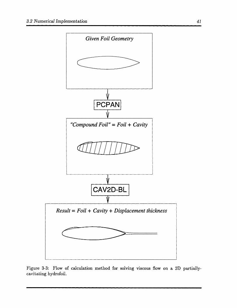
3-3 Flow of calculation method for solving viscous flow on a 2D partially-
cavitating hydrofoil ............................... 41
LIST OF FIGURES
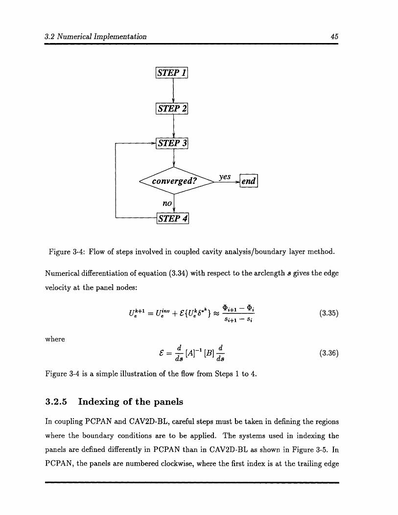
3-4 Flow of steps involved in coupled cavity analysis/boundary layer method. 45
3-5 Index arrangement for PCPAN, SCPAN, and CAV2D-BL. Indices corre-
spond to panel numbers (as opposed to node number). ........... 47
3-6 Convergence characteristics of viscous cavity solution for CL, CD, a.is, and
V/c2 (cavity volume). a = 3.50,1/c = 0.30,N = the number of panels on
the foil and cavity. .............................. 50
3-7 Above: Present method's prediction of heavy foil with viscous effects.
Below: Viscous and inviscid pressure distribution on foil. . ......... 51
3-8 Displacement thickness, momentum thickness, and shape factor along suc-
tion and pressure sides of hydrofoil. a = 3.50,1/c = 0.20 . ........ . 53
3-9 Shape factor along suction side of foil showing the method used to predict
cavity detachment. I/c = 0.20, a = 3.5. ................... 54
3-10 Foil geometry and cavity shape showing the effect of tunnel walls. 'a=0.86 55
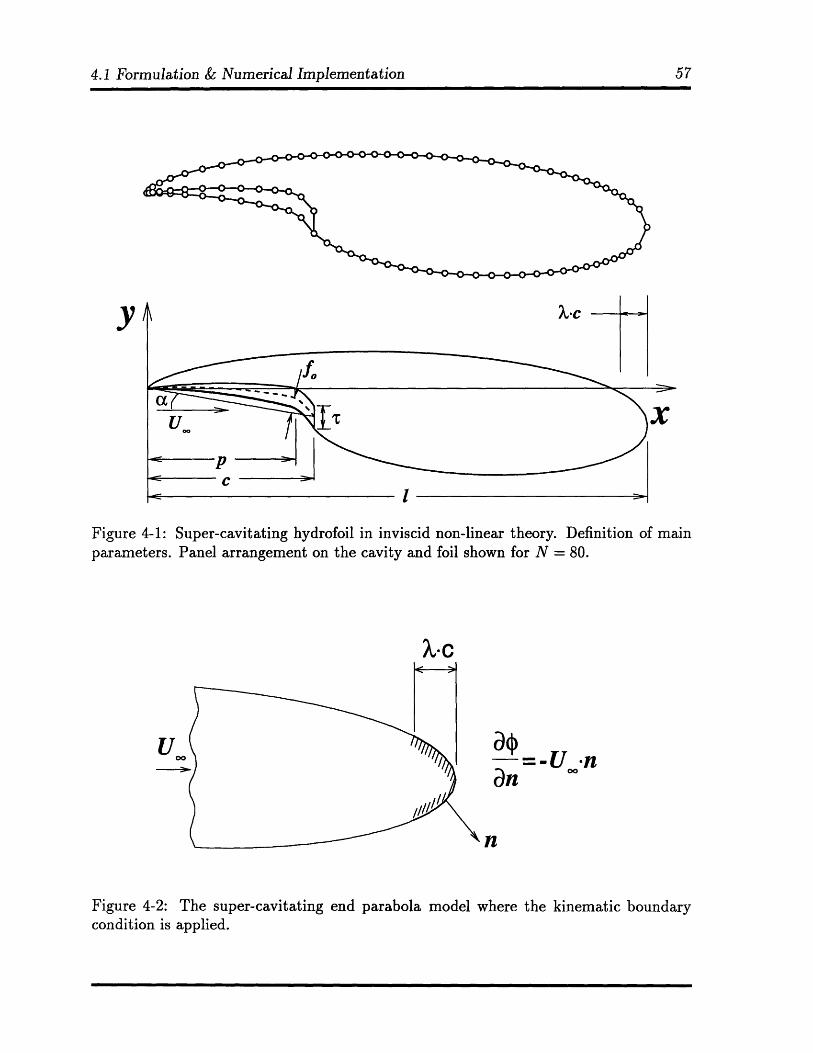
4-1 Super-cavitating hydrofoil in inviscid non-linear theory. Definition of main
parameters. Panel arrangement on the cavity and foil shown for N = 80. 57
4-2 The super-cavitating end parabola model where the kinematic boundary
condition is applied . ............................. 57
4-3 Super-cavitating hydrofoil with its boundary displacement thickness. . . 58
4-4 Super-cavitating hydrofoil in inviscid and viscous flow at Re = 2 x 10⁷.
Cavity shape and boundary layer displacement thickness (top); pressure
distributions (middle); and friction coefficient on the pressure side of the
foil and cavity (bottom). All predicted by the present method ...... . 60
4-5 Cavity length, lift and drag coefficient versus cavitation number for a
super-cavitating hydrofoil at a = 1.50 (left) and a = 3.00 (right), in invis-
cid and viscous flow; predicted by the present method. ........... 62
5-1 Above: the experimental lift coefficient versus the analytical model's pre-
diction for the variety of cavity lengths. Below: the drag coefficient versus
theanalyticalmodel'sprediction. ......................
LIST OF FIGURES
5-2 Velocity measurements along the normal to the cavity surface for cavity
lengths of 1/c = 0.10, 0.20. a = 3.250. (y = 0 corresponds to the cavity
surface location) .. .. .. ... .. .. .. .. ... .. .. .. .. ... . 68
5-3 Velocity measurements along the normal to the cavity surface for cavity
lengths of 1/c = 0.30,0.40. a = 3.250. (y = 0 corresponds to the cavity
surface location) .. .. .. ... .. .. .. .. ... .. .. .. .. ... . 69
5-4 Horizontal and vertical velocities along all sides of a rectangular contour
surrounding the hydrofoil.fully - wetted, a = 3.250............... 71
5-5 Horizontal and vertical velocities along all sides of a rectangular contour
surrounding the hydrofoil.l/c = 0.10, a = 3.5.. . .............. . 72
5-6 Horizontal and vertical velocities along all sides of a rectangular contour
surrounding the hydrofoil.l/c = 0.20, a = 3.5.. . .............. . 73
5-7 Horizontal and vertical velocities along all sides of a rectangular contour
surrounding the hydrofoil.1/c = 0.30, a = 3.50. . .............. . 74
5-8 Top: Boundary layer profiles comparing experiment (circles) and theory
(solid line), x/c = 0.50, fully-wetted, and a = 3.50. Middle: x/c = 0.80.
Bottom: x/c = 0.90. ............................. 75
5-9 Top: Boundary layer profiles comparing experiment (circles) and theory
(solid line), x/c = 0.50, 1/c = 0.10 and a = 3.50. Middle: x/c = 0.80.
Bottom: x/c = 0.90. ............................. 76
5-10 Top: Boundary layer profiles comparing experiment (circles) and theory
(solid line), x/c = 0.50, 1/c = 0.20 and a = 3.50. Middle: x/c = 0.80.
Bottom : x/c = 0.90. .................. ............ 77
5-11 Comparison of cavitation number (pressure coefficient in fully-wetted flow)
between experiment and theory for various cavity lengths. a = 3.250. . . 79
6-1 Top: the current viscous cavity model showing the momentum thickness
along the foil and wake surface. Bottom: the current model with the
proposed jump model. ............................-- - -
LIST OF FIGURES
6-2 Top: preliminary results of the proposed jump model showing the mo-
mentum thickness along the suction side of the foil and wake. Bottom:
velocity profiles showing trends of increasing momentum thickness..... . 86
A-1 A 1 - 2 mm gap in measuring exists between the foil and the closest point
measured. ................................... 91
A-2 Above: The present method fit to a boundary layer profile. Below, result-
ing displacement thickness from present method (shown as a diamond) as
well as viscous flow model's displacement thickness prediction. ...... . 93
C-1 Experimental velocity measurements in the boundary layer region. a =
1.660,fully - wetted .................... .......... 97
C-2 Experimental velocity measurements in the boundary layer region. a =
0.70, fully - wetted. ............................. 98
C-3 Experimental velocity measurements in the boundary layer region. a =
1.660, 10%cavity. ............................... 99
C-4 Experimental velocity measurements in the boundary layer region. a =
1.660, 20%cavity. ............................... 99
C-5 Experimental velocity measurements in the boundary layer region. a =
0.40, fully - wetted. ............................. 100
D-1 Left: the inviscid cavity model with 10% cavity and a = 0.70. Right: the
corresponding pressure distribution. (10% 20% (1.660), 10% (0.70)) . . . 103
D-2 Left: the inviscid model's versatility allows the prediction of two cavities.
10% and 25% cavities a = 0.40 Right: corresponding pressure distribution. 104
D-3 Velocity profiles for both experimental and analytical showing the effect of
transition location on the boundary layer. The measured profile has been
arbitrarily shifted vertically due to the ambiguity in the foil surface. . . . 104
D-4 Prediction of velocity profile in wake for various (pressure-side) transition
locations. a = 1.660, fully - wetted ..................... 105
D-5 Velocity profile comparisons between experiment and viscous model ... 106
D-6 Velocity profile comparisons between experiment and viscous model ... 107
LIST OF FIGURES
D-7 Lift and drag coefficients as a function of transition location,
sure side of the foil. Fully-wetted, a = 0.70. ..........
D-8 Lift and drag coefficients as a function of transition location,
sure side of the foil. Cavity flow, a = 1.660, 1/c = 0.20. . . .
D-9 Lift and drag coefficients as a function of transition location,
sure side of the foil. Cavity flow, a = 0.40, 1/c = 0.45.....
on the pres-
on the pres-
on the pres-
107
108
109
Chapter 1
Introduction
Cavitation is the manifestation of vapor pockets in a flowing liquid owing to a local
minimization of pressure. This phenomenon of liquid vaporization has antagonized the
design of propulsors by causing:
* diminished efficiency/performance
* excessive structural vibration (leading to failure)
* immense material corrosion due to the high forces involved in the bubble collapse
* flow noise
Cavitation is inevitably an issue in the design of efficient high speed pumps and propellers.
Therefore, there is a great interest in studying the physics underlying the nature of
cavitation. Research on cavitation was initiated in pursuit of developing methods to
control cavitation: methods to design more efficient hydrofoils and propellers that use
cavitation to their benefit.
In fact, optimally-cavitating propulsors can be more efficient than those designed to
not cavitate. The presence of the cavity introduces the advantageous quality of having
smaller viscous losses. However, it also introduces undesirable form drag, called cavity
drag. Thus, the design of the most efficient propulsor represents a delicate balance
between two extremes: no cavitation (large blade area with no cavity drag but high
1.1 Research History
viscous losses) or fully-cavitating (small blade area with minimal viscous losses but with
cavity drag).
Computational tools have been of paramount importance in designing cavitating
propulsors. These tools are developed in a systematic manner, starting with simple
two-dimensional geometries in inviscid flow, working towards three-dimensional geome-
tries in viscous flow. The philosophy underlying the development of the codes is to begin
with the simplest model and progressively extend this model to more complicated and
realistic flows. This work represents a small contribution in the efforts to ultimately
develop an automated numerical method for the design of optimum propulsors.
This thesis attempts to address the issue of viscosity in cavitating flow. The effect
of viscosity is studied by performing experiments on simple two-dimensional hydrofoils
in cavitating flow. Knowledge obtained from experiments is then used to further de-
velop existing computational methods to accurately model viscous flow around cavitating
propulsors.
1.1 Research History
1.1.1 Experiments
Experimentation is an essential element in the study of cavitation. It is primarily useful
for understanding the actual physics and details of the flow. A vast number of experiments
have been conducted to investigate cavitation. The purpose in many of these experiments
was to measure the lift, drag, and moment coefficients for various cavitation numbers.
Parkin (1958) measured lift, drag, and pitching moment in cavitating and fully-wetted
flow for flat plate and circular-arc sections. Meijer (1959) measured forces as well as
pressures in the vicinity of the cavity trailing edge of a partially-cavitating hydrofoil.
His experiments indicated essential differences between partially-cavitating and super-
cavitating flows. Wade and Acosta (1966) studied the lift and drag on a plano-convex
foil in the presence of partial and super cavitation. They also observed strong, periodic
oscillations in both cavity length and forces acting on the hydrofoil. A secondary effort of
1.1 Research History
their experiments was to observe the formation and development of the cavity. Uhlman
and Jiang (1977) studied the cavity length, for various cavitation numbers, on a plano-
convex foil. There results were correlated to the theories of Wade (1967) and Geurst
(1959). Maixner (1977) investigated the influence on wall effects on force and moment
coefficients of a super-cavitating hydrofoil. His results were compared to the methods of
Wu, Whitney, and Lin (1971).
Laser Doppler Velocimetry (LDV) measurements in the boundary layer, behind the
cavity of a partially-cavitating hydrofoil, were performed by Kato et al (1987) and Fine
(1988). Kato reported an appreciable increase in the boundary layer thickness due to the
existence of cavitation. Kato also measured the unsteady flow in the presence of cloud
cavitation using a conditional sampling technique. Lurie(1993) measured the formation
of the unsteady boundary layer on a fully-wetted hydrofoil subject to sinusoidal gust (the
Flapping Foil Experiment), in addition to unsteady pressures on the foil surface.
Kinnas and Mazel (1993) performed LDV measurements about a super-cavitating
hydrofoil. They measured velocities near the cavity surface to calculate the cavitation
number. Measurements were also made along a rectangular contour surrounding the foil
and cavity. These measurements were used with momentum integrations to calculate the
lift and drag forces acting on the hydrofoil. A list of earlier super-cavitating experiments
is given in Kinnas and Mazel (1993).
1.1.2 Numerical Methods
Many codes have been developed over the past few years to aid the designer in developing
optimal blade geometries. A history of numerical methods used to model sheet cavitation
is given in Villeneuve (1993). The nonlinear perturbation potential method by Kinnas
and Fine (1990) laid the groundwork for the viscous cavity model, P2DBLWC.
Villeneuve's viscous cavity analysis method was based on Drela's (1989) airfoil anal-
ysis code, XFOIL, which uses an interactive viscous-inviscid approach to solving the flow
around airfoils. Drela's work was further developed by Hufford (1992) who applied the
boundary layer method in a strip-wise sense to analyze the viscous flow around three-
dimensional propeller blades. In doing this, Hufford coupled the viscous routines of
1.1 Research History
Figure 1-1: History of code development for two-dimensional cavitating boundary layersolver.
XFOIL to the inviscid perturbation potential method of PAN2D. 1 The history of the
code is illustrated in Figure 1-1.
The scope of Villeneuve's work was divided into two strands: numerical and exper-
imental. The numerical method, P2DBLWC, was based on Hufford's code, PAN2D-
BL. To model the cavity, Villeneuve used a similar method to that used in boundary
layer theory, where blowing sources were used to represent the cavity. This method is
referred to as the "thin" cavity method, in which case both the cavity and the displace-
ment thickness are assumed to be "small" with respect to the cavity length. Villeneuve's
work also included the implementation of the method of images to account for the effects
of tunnel walls.
To validate P2DBLWC, Villeneuve performed experiments on a partially-cavitating
hydrofoil. In correlating experimental results with numerical predictions, he compared
IXFOIL uses a linear vorticity streamfunction formulation for inviscid flow (Drela, 1989).
1.2 Objectives
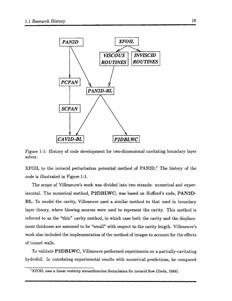
P2DBLWC: 'Thin" cavity approach CAV2D-BL: Nonlinear cavity approach_. _ C•f--A* n--n
'-I-',,F
Figure 1-2: Hydrofoil with cavity and displacement thickness illustrating where boundaryconditions are applied.
integral parameters, such as the boundary layer displacement and momentum thickness,
as well as lift and drag coefficients. The predicted results by the analysis method were
shown to be in good agreement with the experimental results.
1.2 Objectives
This thesis serves to continue Villeneuve's efforts to model viscous flow around cavitat-
ing hydrofoils. Instead of comparing integral parameters, such as the boundary layer
displacement and momentum thickness (as Villeneuve did), the results herein compare
actual velocities, which are predicted anywhere in the flowfield, with those from experi-
ments. In doing this, a numerical method was developed to extract velocity profiles from
the integral quantities given as a result of the boundary layer solver.
The secondary goal of this work lies in further developing the code P2DBLWC:
increasing the versatility and robustness of the boundary layer solver used to model
viscous cavitating hydrofoils.
To this end, the following improvements were made to P2DBLWC:
* The non-linear cavity method: The boundary layer is solved on the cavity surface
resulting from "fully" non-linear cavity analysis.
* Implement a new spacing technique, blended spacing, which allows the user to spec-
ify the cavity detachment location exactly and ensures continuous panel spacing.
1.2 Objectives
* Extend the method to super-cavitating sections.
* Fix bugs in the old code.
* Formulate and implement the "momentum jump" model which models the in-
creased momentum and displacement thickness which occurs at the trailing edge
of the cavity (as evidenced by experiments).
Villeneuve's "thin" cavity method, P2DBLWC, has been shown to work well when
the cavity is very thin compared to the foil thickness. In his method, he represents the
cavity and boundary layer by using blowing sources applied on the cavity surface as
shown in Figure 1-2. In this thesis, however, a different approach is used to model the
viscous flow around the cavity, namely, the nonlinear cavity approach, as shown in Figure
1-2. First, the cavity is generated in nonlinear theory, then the boundary conditions are
applied on the boundary surrounding the union of the cavity and foil surface. However,
the present method does not ensure that the dynamic boundary condition, requiring the
pressure to be constant on the cavity surface, is completely satisfied. The present method
only performs the first iteration of the inviscid/viscous coupling procedure. Kinnas et al
(1994) performed a second iteration of the present method, which showed not the affect
the results drastically.
The code incorporating these changes has been named CAV2D-BL - a two-dimensional
cavitating boundary layer solver.
I
Chapter 2
Experiment
The purpose of the partially-cavitating hydrofoil experiments (PACHE) is to acquire data
which can be used to validate the coupled nonlinear cavity analysis method (PCPAN)
and boundary layer solver (CAV2D-BL). Also of interest in these experiments is the
study of how the cavity drag manifests itself into the wake. To fulfill these goals, velocity
measurements and pressure measurements (cavitation numbers) were taken for various
angles of attack and cavitation numbers.
PACHE was performed in three phases. The subsequent phases were necessary to
fix problems in the previous phases. The following outline describes each phase of the
experiment:
* Phase I:
- Performed by: Shige Mishima, Cedric Savineau, Wesley Brewer, and Platon
Velonias
- Problems:
* Fiber-optic beam was not working. Boundary layer measurements could
only be taken with horizontal component of laser.
* No turbulator strip on pressure side of foil introduced error in the predic-
tion of the transition location.
* Phase II:
2.1 Setup
- Performed by: Wesley Brewer
- Corrections since phase I:
* Fiber-optic beam fixed.
* Turbulator strip placed on pressure side of foil.
- Phase II problems: Pressure measurements could not be taken because manome-
ter was not working correctly.
* Phase III:
- Performed by: Wesley Brewer
- Corrections since phase II: Manometer fixed
- Phase III Problems: Manometer still not completely accurate.
2.1 Setup
The experiments were performed in the MIT Variable Pressure Water Tunnel (Kerwin,
1992). The tunnel has a twenty inch square testing cross-section enveloped on all sides by
plexiglass windows. First, the tunnel was de-aired at low speeds using the vacuum pump;
then, the pressure was dropped below the point of cavitation inception. One impeller,
driven by a 75 horsepower motor, propels the water through the closed-loop tunnel at
speeds up to 9 m/s (30 ft/s); a speed of 8 m/s (25 ft/s) was used for this experiment.
Figure 2-1 shows the experimental setup. The foil, a "heavy" symmetrical stainless-
steel foil, has a chord of twelve inches and a span of twenty inches. The maximum
thickness to chord ratio is twelve percent at half-chord. A turbulator strip was placed
on the pressure side of the foil at 1/5 chord. Two rubber gaskets, squeezed in between
the plexiglass window and the foil, served to prevent any secondary flow between the
pressure and suction side. The foil was mounted on the vertical plexi-glass walls at two
points on each side, as shown in Figure 2-1. A stainless-steel pin, set at approximately
3/4 chord, was used to adjust the angle of attack.
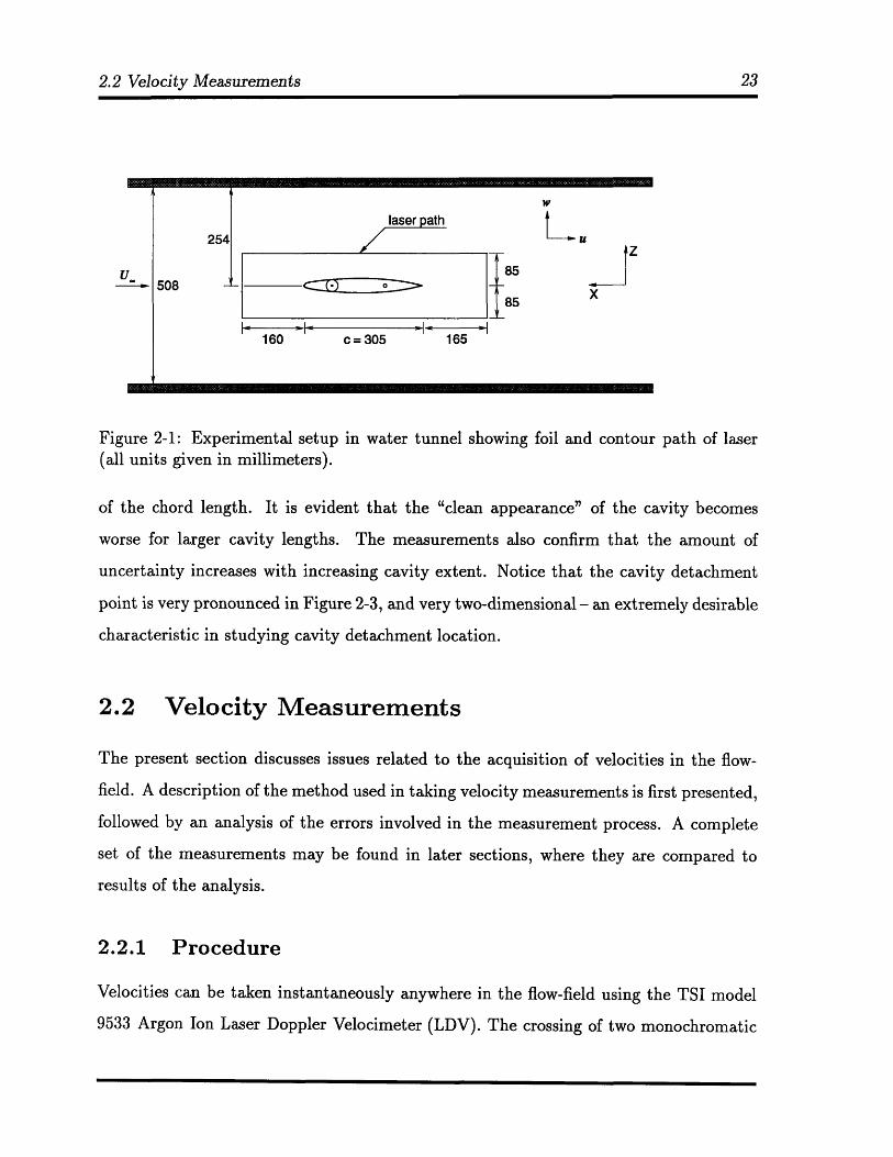
Figure 2-3 shows actual photographs of the cavitating hydrofoil in the testing section
of the water tunnel. The top photo shows a very stable sheet cavity of extent 10%
2.2 Velocity Measurements
U.
254
2.
w
Uz
xi
160 c = 305 165
Figure 2-1: Experimental setup in water tunnel showing foil and contour path of laser(all units given in millimeters).
of the chord length. It is evident that the "clean appearance" of the cavity becomes
worse for larger cavity lengths. The measurements also confirm that the amount of
uncertainty increases with increasing cavity extent. Notice that the cavity detachment
point is very pronounced in Figure 2-3, and very two-dimensional - an extremely desirable
characteristic in studying cavity detachment location.
2.2 Velocity Measurements
The present section discusses issues related to the acquisition of velocities in the flow-
field. A description of the method used in taking velocity measurements is first presented,
followed by an analysis of the errors involved in the measurement process. A complete
set of the measurements may be found in later sections, where they are compared to
results of the analysis.
2.2.1 Procedure
Velocities can be taken instantaneously anywhere in the flow-field using the TSI model
9533 Argon Ion Laser Doppler Velocimeter (LDV). The crossing of two monochromatic
mm 11~·1~·1~111111·1·1111·111~
vvv
2.2 Velocity Measurements
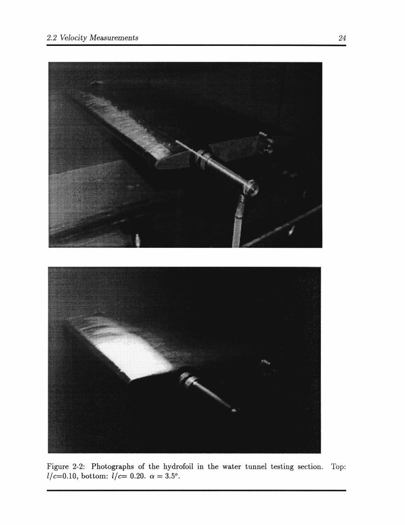
Figure 2-2: Photographs of the hydrofoil in the water tunnel testing section. Top:l/c=0.10, bottom: l/c= 0.20. a = 3.5' .
2.2 Velocity Measurements
Figure 2-3: Photographs of the hydrofoil in the water tunnel testing section. Top:l/c=0.30, l/c=0.40. a = 3.50 .
2.2 Velocity Measurements
beams creates an interference fringe pattern. Seed particles' in the flow create a distur-
bance in the fringe pattern; this disturbance is measured by a photodetector and then
processed through digital signal analyzers, ultimately resulting in a velocity reading. A
two-component optical laser was used in all phases of the experiment to measure velocities
along the rectangular contour. In Phase I of the experiment, boundary layer velocities
were acquired by the horizontal component of the laser (which cannot measure velocities
within 1 - 3 mm of the foil surface). However in Phase II, boundary layer measurements
were taken by a rotatable fiber-optic beam which measured velocities parallel to the foil
surface.
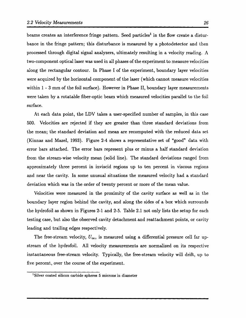
At each data point, the LDV takes a user-specified number of samples, in this case
500. Velocities are rejected if they are greater than three standard deviations from
the mean; the standard deviation and mean are recomputed with the reduced data set
(Kinnas and Mazel, 1993). Figure 2-4 shows a representative set of "good" data with
error bars attached. The error bars represent plus or minus a half standard deviation
from the stream-wise velocity mean (solid line). The standard deviations ranged from
approximately three percent in inviscid regions up to ten percent in viscous regions
and near the cavity. In some unusual situations the measured velocity had a standard
deviation which was in the order of twenty percent or more of the mean value.
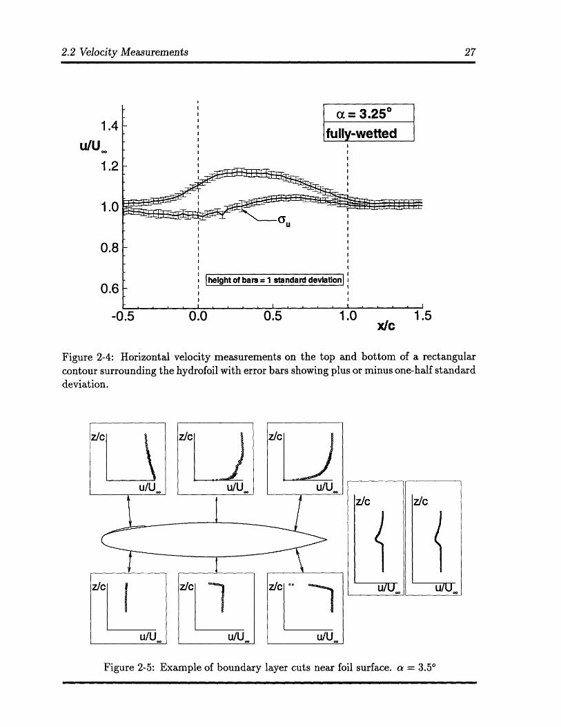
Velocities were measured in the proximity of the cavity surface as well as in the
boundary layer region behind the cavity, and along the sides of a box which surrounds
the hydrofoil as shown in Figures 2-1 and 2-5. Table 2.1 not only lists the setup for each
testing case, but also the observed cavity detachment and reattachment points, or cavity
leading and trailing edges respectively.
The free-stream velocity, U,,, is measured using a differential pressure cell far up-
stream of the hydrofoil. All velocity measurements are normalized on its respective
instantaneous free-stream velocity. Typically, the free-stream velocity will drift, up to
five percent, over the course of the experiment.
'Silver coated silicon carbide spheres 5 microns in diameter
2.2 Velocity Measurements
1.4u/U
1.2
1.0
0.8
0.6
-C
II
I
I
I height of bars = 1 standard deviation)I
0.0 0.5 1.0xIc
Figure 2-4: Horizontal velocity measurements on the top and bottom of a rectangularcontour surrounding the hydrofoil with error bars showing plus or minus one-half standarddeviation.
z/c z/cI
Figure 2-5: Example of boundary layer cuts near foil surface. a = 3.50
I
2.2 Velocity Measurements
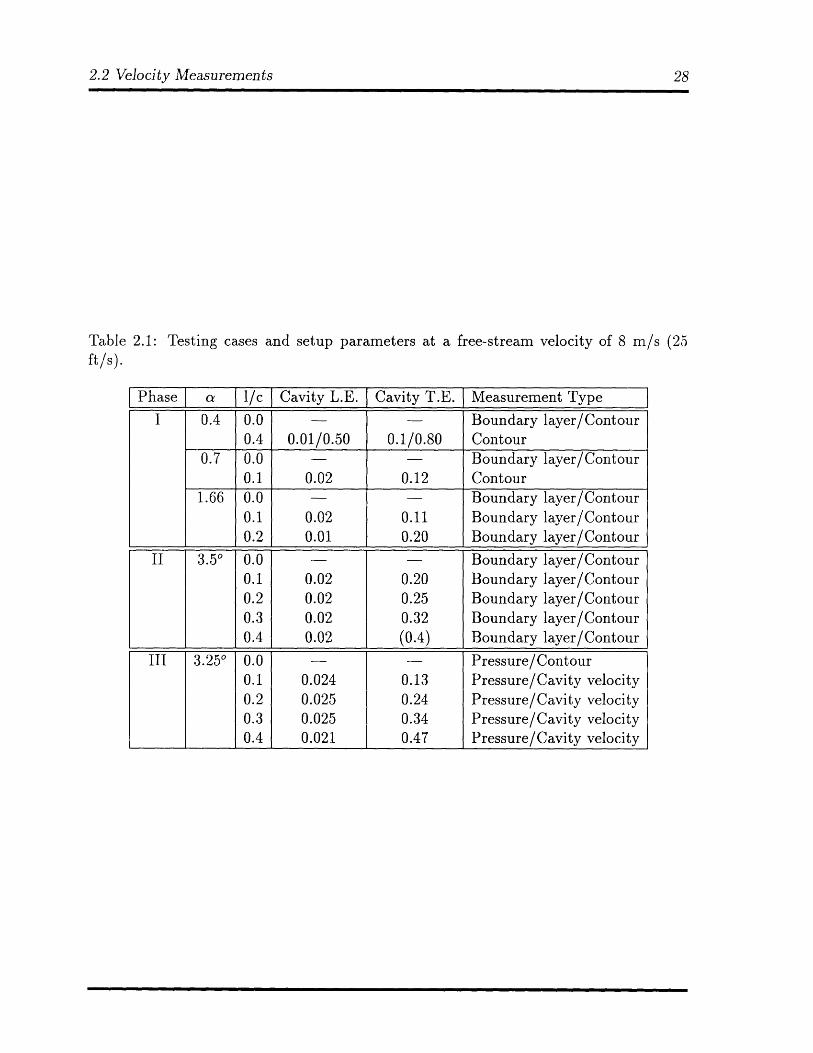
Table 2.1:ft/s).
Testing cases and setup parameters at a free-stream velocity of 8 m/s (25
Phase a l1/c Cavity L.E. Cavity T.E. Measurement Type
I 0.4 0.0 - - Boundary layer/Contour0.4 0.01/0.50 0.1/0.80 Contour
0.7 0.0 - - Boundary layer/Contour0.1 0.02 0.12 Contour
1.66 0.0 - - Boundary layer/Contour0.1 0.02 0.11 Boundary layer/Contour0.2 0.01 0.20 Boundary layer/Contour
II 3.50 0.0 - - Boundary layer/Contour0.1 0.02 0.20 Boundary layer/Contour0.2 0.02 0.25 Boundary layer/Contour0.3 0.02 0.32 Boundary layer/Contour0.4 0.02 (0.4) Boundary layer/Contour
III 3.250 0.0 - - Pressure/Contour0.1 0.024 0.13 Pressure/Cavity velocity0.2 0.025 0.24 Pressure/Cavity velocity0.3 0.025 0.34 Pressure/Cavity velocity0.4 0.021 0.47 Pressure/Cavity velocity
_ _
2.2 Velocity Measurements
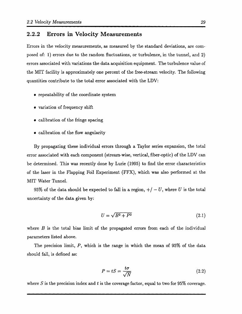
2.2.2 Errors in Velocity Measurements
Errors in the velocity measurements, as measured by the standard deviations, are com-
posed of: 1) errors due to the random fluctuations, or turbulence, in the tunnel, and 2)
errors associated with variations the data acquisition equipment. The turbulence value of
the MIT facility is approximately one percent of the free-stream velocity. The following
quantities contribute to the total error associated with the LDV:
* repeatability of the coordinate system
* variation of frequency shift
* calibration of the fringe spacing
* calibration of the flow angularity
By propagating these individual errors through a Taylor series expansion, the total
error associated with each component (stream-wise, vertical, fiber-optic) of the LDV can
be determined. This was recently done by Lurie (1995) to find the error characteristics
of the laser in the Flapping Foil Experiment (FFX), which was also performed at the
MIT Water Tunnel.
95% of the data should be expected to fall in a region, +/ - U, where U is the total
uncertainty of the data given by:
U = ,/B 2 + P2 (2.1)
where B is the total bias limit of the propagated errors from each of the individual
parameters listed above.
The precision limit, P, which is the range in which the mean of 95% of the data
should fall, is defined as:
P = tS = (2.2)
where S is the precision index and t is the coverage factor, equal to two for 95% coverage.
2.3 Pressure Measurements
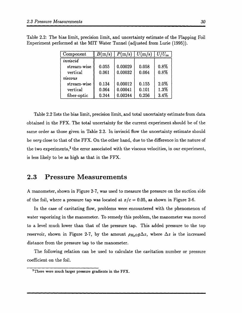
Table 2.2: The bias limit, precision limit, and uncertainty estimate of the Flapping FoilExperiment performed at the MIT Water Tunnel (adjusted from Lurie (1995)).
Component B(m/s) P(m/s) U(m/s) U/Uooinviscid
stream-wise 0.055 0.00029 0.058 0.8%vertical 0.061 0.00032 0.064 0.8%
viscousstream-wise 0.134 0.00012 0.155 2.0%vertical 0.064 0.00041 0.101 1.3%fiber-optic 0.244 0.00244 0.256 3.4%
Table 2.2 lists the bias limit, precision limit, and total uncertainty estimate from data
obtained in the FFX. The total uncertainty for the current experiment should be of the
same order as those given in Table 2.2. In inviscid flow the uncertainty estimate should
be very close to that of the FFX. On the other hand, due to the difference in the nature of
the two experiments,2 the error associated with the viscous velocities, in our experiment,
is less likely to be as high as that in the FFX.
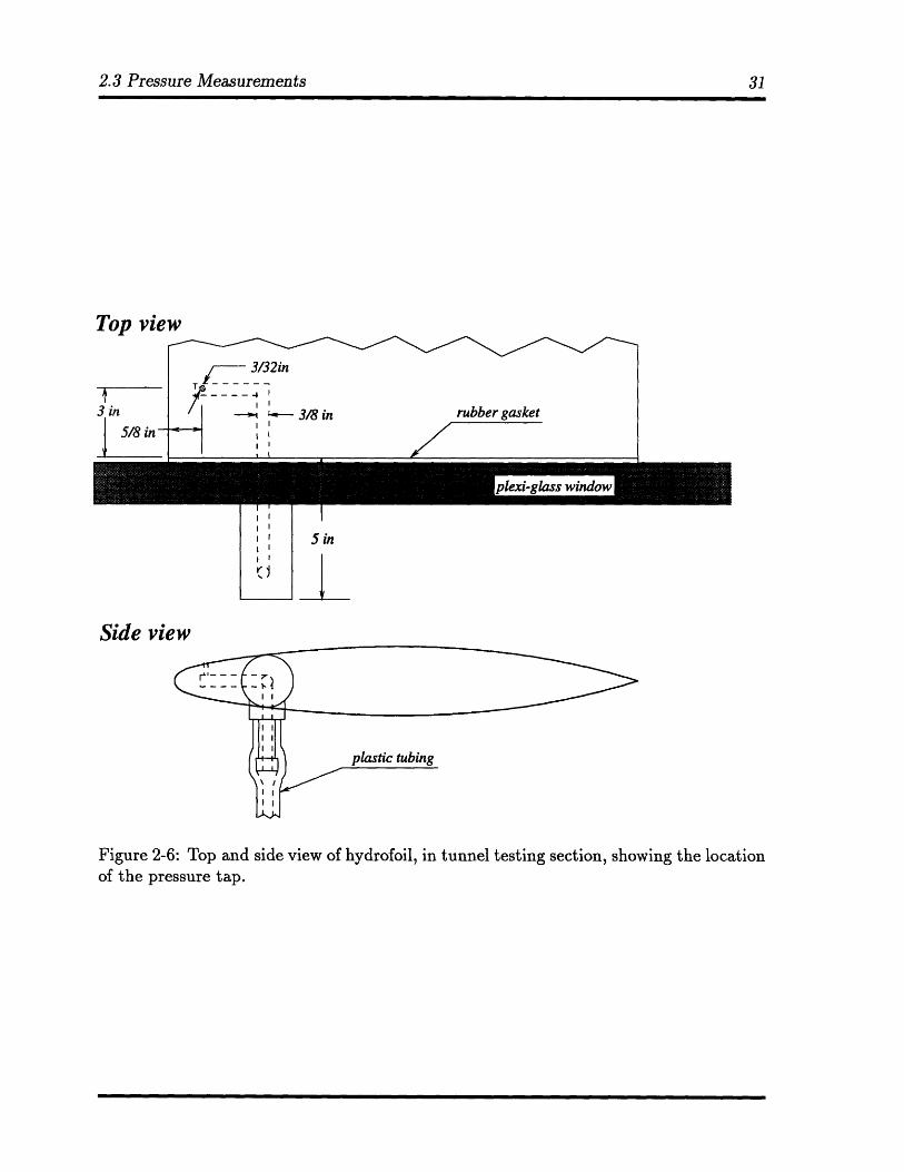
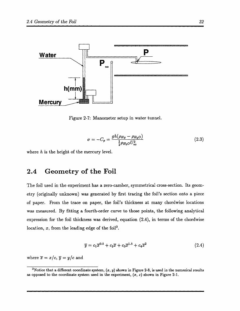
2.3 Pressure Measurements
A manometer, shown in Figure 2-7, was used to measure the pressure on the suction side
of the foil, where a pressure tap was located at x/c = 0.05, as shown in Figure 2-6.
In the case of cavitating flow, problems were encountered with the phenomenon of
water vaporizing in the manometer. To remedy this problem, the manometer was moved
to a level much lower than that of the pressure tap. This added pressure to the top
reservoir, shown in Figure 2-7, by the amount pHogAz, where Az is the increased
distance from the pressure tap to the manometer.
The following relation can be used to calculate the cavitation number or pressure
coefficient on the foil.
2There were much larger pressure gradients in the FFX.
2.3 Pressure Measurements
Top view
5 in
Side view
Figure 2-6: Top and side view of hydrofoil, in tunnel testing section, showing the locationof the pressure tap.
2.4 Geometry of the Foil
Me
P
Figure 2-7: Manometer setup in water tunnel.
gh(pHg - PH20o)o = -CP 1 PH
2PH20oo(2.3)
where h is the height of the mercury level.
2.4 Geometry of the Foil
The foil used in the experiment has a zero-camber, symmetrical cross-section. Its geom-
etry (originally unknown) was generated by first tracing the foil's section onto a piece
of paper. From the trace on paper, the foil's thickness at many chordwise locations
was measured. By fitting a fourth-order curve to those points, the following analytical
expression for the foil thickness was derived, equation (2.4), in terms of the chordwise
location, x, from the leading edge of the foil3 .
Y = cy. + C2X + C3'1 5 + C4Y 2 (2.4)
where Y = x/c, V = y/c and
3Notice that a different coordinate system, (x, y) shown in Figure 2-8, is used in the numerical resultsas opposed to the coordinate system used in the experiment, (x, z) shown in Figure 2-1.
b~d~a8n~
ymný~5
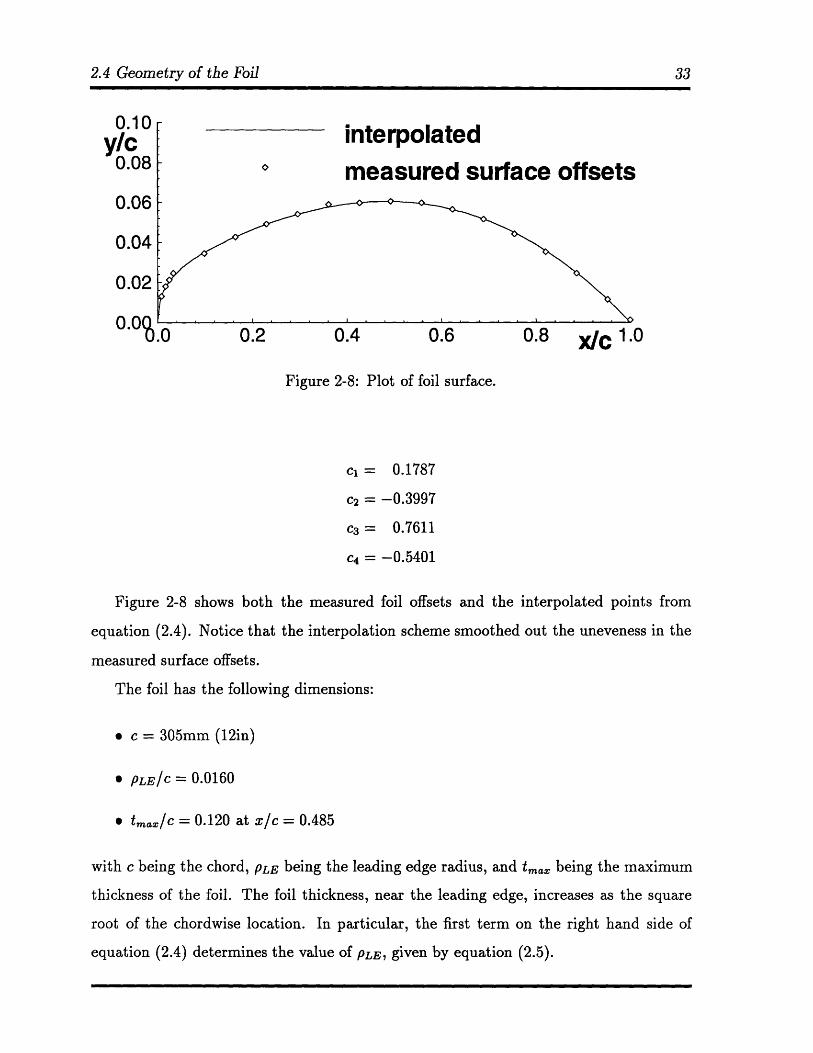
2.4 Geometry of the Foil
f~ .d f~U. IU
ylc0.08
0.06
0.04
0.02
n 0n' .0 0.2 0.4 0.6 0.8 X/C 1.0
Figure 2-8: Plot of foil surface.
cl = 0.1787
c2 = -0.3997
c3 = 0.7611
c4= -0.5401
Figure 2-8 shows both the measured foil offsets and the interpolated points from
equation (2.4). Notice that the interpolation scheme smoothed out the uneveness in the
measured surface offsets.
The foil has the following dimensions:
* c = 305mm (12in)
* PLEIC = 0.0160
* tmax/c = 0.120 at x/c = 0.485
with c being the chord, PLE being the leading edge radius, and tmax being the maximum
thickness of the foil. The foil thickness, near the leading edge, increases as the square
root of the chordwise location. In particular, the first term on the right hand side of
equation (2.4) determines the value of PLE, given by equation (2.5).
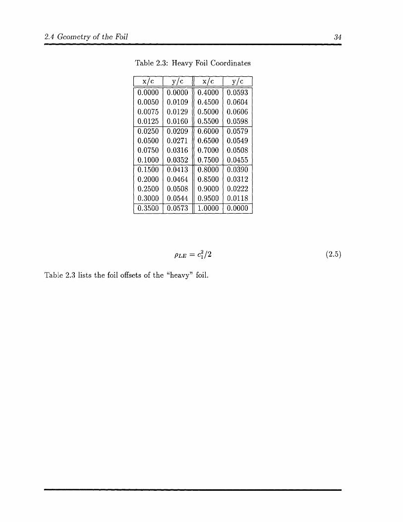
Table 2.3: Heavy Foil Coordinates
x/c y/c x/c y/c0.0000 0.0000 0.4000 0.05930.0050 0.0109 0.4500 0.06040.0075 0.0129 0.5000 0.06060.0125 0.0160 0.5500 0.05980.0250 0.0209 0.6000 0.05790.0500 0.0271 0.6500 0.05490.0750 0.0316 0.7000 0.05080.1000 0.0352 0.7500 0.04550.1500 0.0413 0.8000 0.03900.2000 0.0464 0.8500 0.03120.2500 0.0508 0.9000 0.02220.3000 0.0544 0.9500 0.01180.3500 0.0573 1.0000 0.0000
PLE = c /2
Table 2.3 lists the foil offsets of the "heavy" foil.
2.4 Geometry of the Foil
(2.5)
I-
Chapter 3
CAV2D-BL: Partially-Cavitating
Boundary Layer Solver
3.1 Formulation
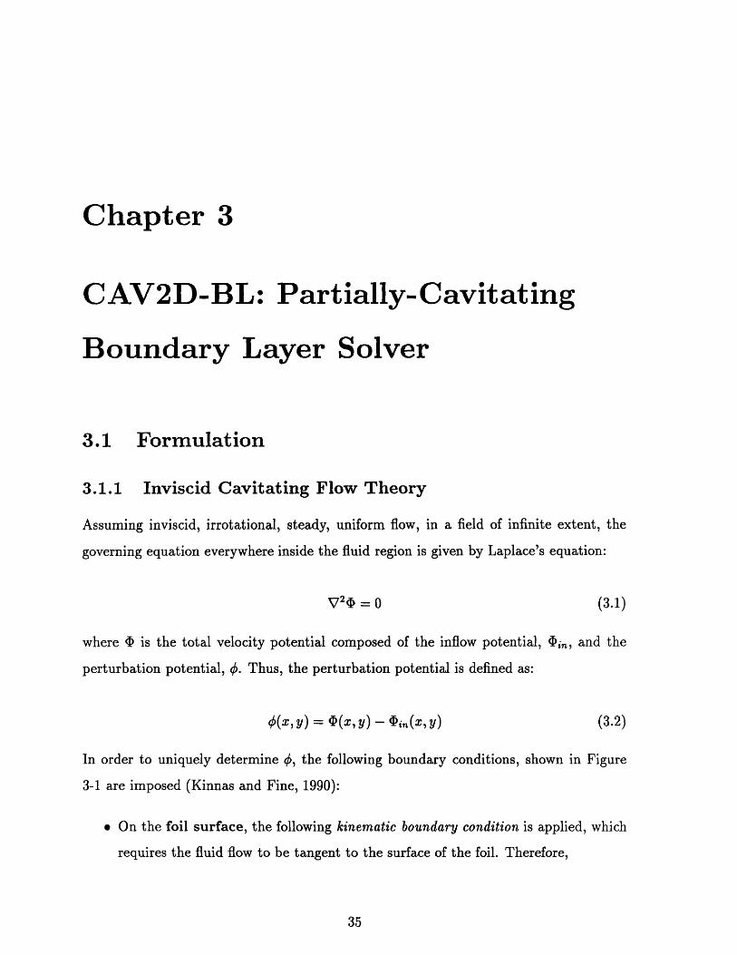
3.1.1 Inviscid Cavitating Flow Theory
Assuming inviscid, irrotational, steady, uniform flow, in a field of infinite extent, the
governing equation everywhere inside the fluid region is given by Laplace's equation:
V2 D = 0 (3.1)
where 4 is the total velocity potential composed of the inflow potential, 4in, and the
perturbation potential, q. Thus, the perturbation potential is defined as:
0(X, y) = #(x, y) - i,n(X, y) (3.2)
In order to uniquely determine 0, the following boundary conditions, shown in Figure
3-1 are imposed (Kinnas and Fine, 1990):
* On the foil surface, the following kinematic boundary condition is applied, which
requires the fluid flow to be tangent to the surface of the foil. Therefore,
P = PV =-U -n
Vý.<oo VO. -+ o
0
Figure 3-1: Hydrofoil with imposed boundary conditions.
S=-Uoo non
where n is the surface unit normal vector.
* At infinity the perturbation velocities should go to zero.
V --+ 0 (3.4)
* The Kutta condition requires finite velocities at the trailing edge of the foil:
V¢ < oo (3.5)
* The dynamic boundary condition specifies constant pressure on the cavity:
Iql I = U00ooi + (3.6)
* Near the trailing edge of the cavity, a pressure recovery termination model
replaces equation (3.6):
IqtI = Uoov /i+[1 - f(x)]
3.1 Formulation
(3.3)
U=
(3.7)
3.1 Formulation
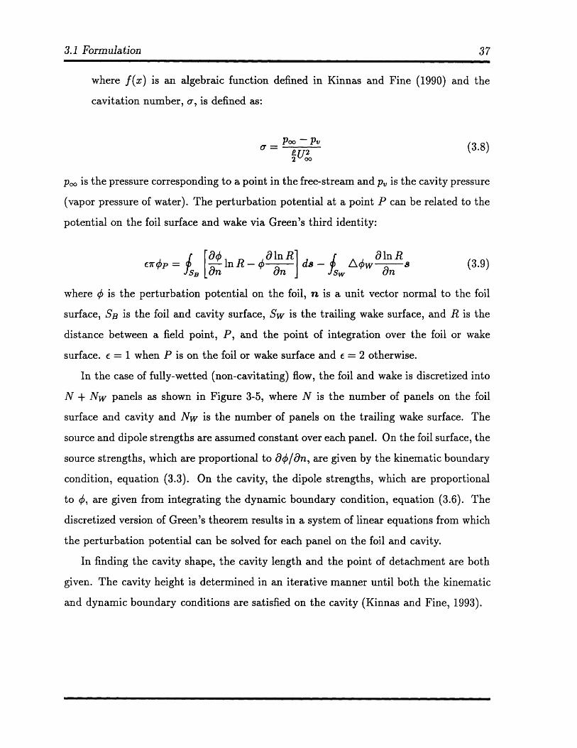
where f(x) is an algebraic function defined in Kinnas and Fine (1990) and the
cavitation number, o0, is defined as:
poo - p,Po- - P(3.8)2
p0 is the pressure corresponding to a point in the free-stream and p, is the cavity pressure
(vapor pressure of water). The perturbation potential at a point P can be related to the
potential on the foil surface and wake via Green's third identity:
erp = InR - dIn d -w ln R (3.9)= an sw -n7
where q is the perturbation potential on the foil, n is a unit vector normal to the foil
surface, SB is the foil and cavity surface, Sw is the trailing wake surface, and R is the
distance between a field point, P, and the point of integration over the foil or wake
surface. c = 1 when P is on the foil or wake surface and e = 2 otherwise.
In the case of fully-wetted (non-cavitating) flow, the foil and wake is discretized into
N + Nw panels as shown in Figure 3-5, where N is the number of panels on the foil
surface and cavity and Nw is the number of panels on the trailing wake surface. The
source and dipole strengths are assumed constant over each panel. On the foil surface, the
source strengths, which are proportional to Oq/dn, are given by the kinematic boundary
condition, equation (3.3). On the cavity, the dipole strengths, which are proportional
to 0, are given from integrating the dynamic boundary condition, equation (3.6). The
discretized version of Green's theorem results in a system of linear equations from which
the perturbation potential can be solved for each panel on the foil and cavity.
In finding the cavity shape, the cavity length and the point of detachment are both
given. The cavity height is determined in an iterative manner until both the kinematic
and dynamic boundary conditions are satisfied on the cavity (Kinnas and Fine, 1993).
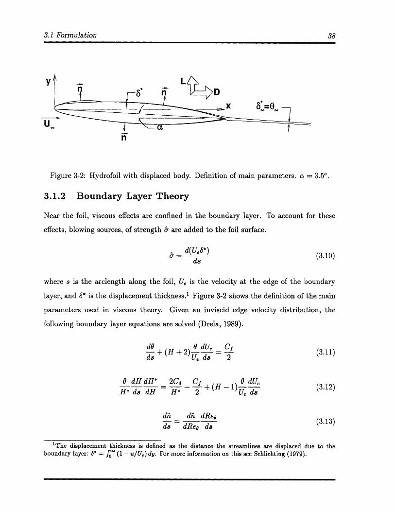
3.1 Formulation
U0
Figure 3-2: Hydrofoil with displaced body. Definition of main parameters. a = 3.50 .
3.1.2 Boundary Layer Theory
Near the foil, viscous effects are confined in the boundary layer. To account for these
effects, blowing sources, of strength & are added to the foil surface.
d(Ue *)ds
(3.10)
where s is the arclength along the foil, U, is the velocity at the edge of the boundary
layer, and 8* is the displacement thickness.' Figure 3-2 shows the definition of the main
parameters used in viscous theory. Given an inviscid edge velocity distribution, the
following boundary layer equations are solved (Drela, 1989).
dO a dUed + (H + 2) 0 dds U, ds (3.11)
0 dH dH* 2 Cd C + (HH* ds dH H* 2
0 dUeUe1) ds (3.12)
(3.13)
'The displacement thickness is defined as the distance the streamlines are displaced due to theboundary layer: 6* = fo (1 - u/Ue) dy. For more information on this see Schlichting (1979).
dfi di~ dReods dReo ds
vlr L 4 ý
3.2 Numerical Implementation
_ dC, f4. Cy Hk__ 1 dUec d,. = 5.6 V' C12] + 25 x [ ( ) 2 ] - (3.14)Cr ds [CrEQ 38* 2 6.7Hk U, d
In the case of laminar flow, equations (3.11), (3.12), and (3.13) are solved for the
quantities 6"*, 0, and hi. For turbulent flow, equations (3.11), (3.12), and (3.14) are solved
for the quantities 6*, 0, and C,.
The inviscid flow is coupled with the viscous flow via the wall transpiration model.
This model gives the edge velocity at each panel in terms of the inviscid edge velocity
and a mass defect term, m = Ue *.2
Ue = U'"" + E{UeS*} (3.15)
The boundary layer equations are solved first with the edge velocity distribution
given from inviscid theory. Once 6* is found, Ue is updated via equation (3.15). The
boundary layer equations are then solved again. This process continues until convergence
is achieved.
This method is extended to partially-cavitating hydrofoils by ignoring the two-phase
flow near the cavity surface, treating the fluid/vapor interface as constant-pressure, free
streamlines, and forcing Cf to zero on the cavity surface (Villeneuve, 1993; Kinnas et al.,
1994). The boundary layer equations are integrated over the non-linear cavity and foil
surface.
3.2 Numerical Implementation
The details of the numerics used to model viscous flow around a partially-cavitating
hydrofoil are given in the following three steps. Figure 3-3 illustrates the different stages
involved in the calculation.
2 E is a geometry-dependent operator, the discretized version of which is given in Section 3.2.2 (Huf-ford, 1990; Drela, 1989).
3.2 Numerical Implementation 40
3.2.1 Step 1: Calculate the cavity height (PCPAN)
Given a hydrofoil geometry, the first step is to calculate the cavity height. This is
accomplished by running PCPAN, the partially-cavitating panel method, which solves
for the inviscid cavity flow in non-linear theory (Kinnas and Fine, 1990).
In PCPAN, the user must specify the cavity leading and trailing edge. The method
solves the inviscid flow in an iterative manner, by updating the cavity height until both
the kinematic boundary condition and dynamic boundary condition are satisfied on the
cavity. PCPAN gives as its result the cavity ordinates and the cavitation number.
3.2.2 Step 2: Calculate inviscid edge velocity on compound
foil (CAV2D-BL)
The next step involves using the loci of points which envelope both the cavity and foil
surface, as shown in Figure 3-3, as a new foil: the "compound" foil.
Discretize Green's third identity, equation (3.9), into N panels to get (Hufford, 1990):
r = n - Dijgj - AAOWi (3.16)j=1 j=1
where
D Jsf F a In R ,
Sij = In Rds
Wi = aInR ds
(3.17)
Dij is an influence function on i due to the jth dipole; Sij is an influence function on i
due to the jth source. Wij is the contribution of source strength from the wake and SCF
is the surface bounded by the union of the foil and cavity surface. The Kutta condition,
equation (3.5), reduces to Morino's condition:
3.2 Numerical Implementation
PCPAN
CAV2D-BL
Figure 3-3: Flow of calculation method for solving viscous flow on a 2D partially-cavitating hydrofoil.
Given Foil Geometry
"Compound Foil" = Foil + Cavity
Result = Foil + Cavity + Displacement thickness
3.2 Numerical Implementation
An, = ON - €1 (3.18)
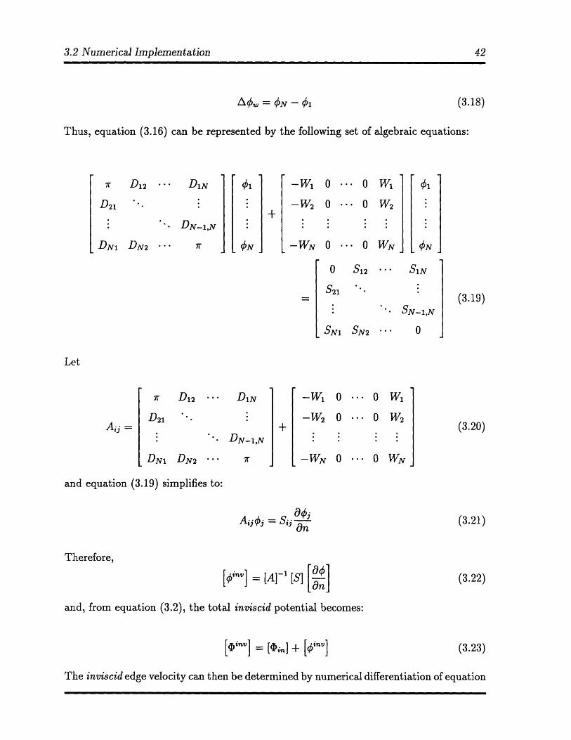
Thus, equation (3.16) can be represented by the following set of algebraic equations:
... DIN
. DN-1,N
DN2
-W1
-W 2
-WN
0 ... 0 W1
o ... 0 W2
0 ... 0 WN
0 S12 ...
S21
• o
SNm SN2
W D12 DiN
DN-1,N
DNi DN2
-W1 0 ... 0 W1
o ... 0 W2
- WN 0 ... 0 WN
and equation (3.19) simplifies to:
Ai¢j = Sij ' -O n
Therefore,
inv = [A]-' [S] an
and, from equation (3.2), the total inviscid potential becomes:
[inv] = [4,l [+inv]
The inviscid edge velocity can then be determined by numerical differentiation of equation
7r
D21
DN1
Let
SiN
SN-1,N
0
(3.19)
(3.20)
(3.21)
(3.22)
(3.23)
- - -
- W2
3.2 Numerical Implementation
(3.23) as such:
d18nv [4 inv]+ - [sinv]ie ds Si+1 - Si
(3.24)
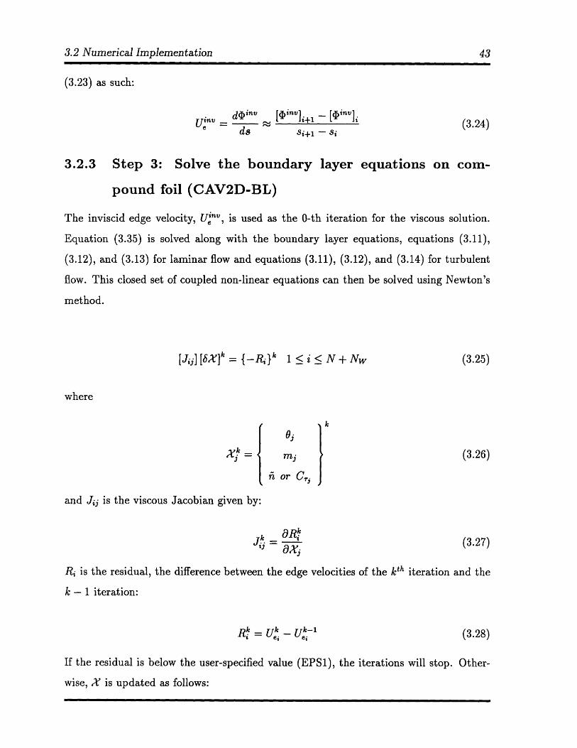
3.2.3 Step 3: Solve the boundary layer equations on com-
pound foil (CAV2D-BL)
The inviscid edge velocity, UinV, is used as the 0-th iteration for the viscous solution.
Equation (3.35) is solved along with the boundary layer equations, equations (3.11),
(3.12), and (3.13) for laminar flow and equations (3.11), (3.12), and (3.14) for turbulent
flow. This closed set of coupled non-linear equations can then be solved using Newton's
method.
[Ji [SX]k = - R , } k 1<i< N+Nw
where
and Jij is the viscous Jacobian given by:
0j
jor
ni or C,
S= ax-j
(3.25)
(3.26)
(3.27)
Ri is the residual, the difference between the edge velocities of the kth iteration and the
k - 1 iteration:
R• = U, -- Ue- 1 (3.28)
If the residual is below the user-specified value (EPS1), the iterations will stop. Other-
wise, X is updated as follows:
3.2 Numerical Implementation
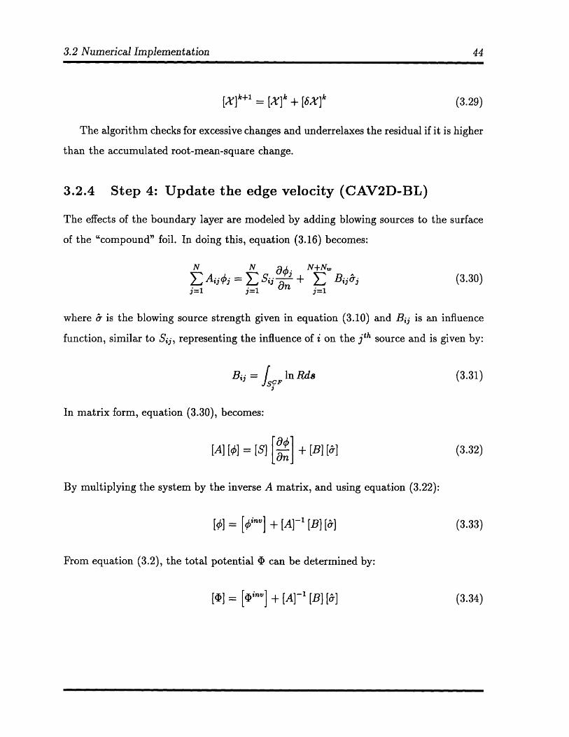
[X]k+l = [X]k + [SX]k (3.29)
The algorithm checks for excessive changes and underrelaxes the residual if it is higher
than the accumulated root-mean-square change.
3.2.4 Step 4: Update the edge velocity (CAV2D-BL)
The effects of the boundary layer are modeled by adding blowing sources to the surface
of the "compound" foil. In doing this, equation (3.16) becomes:
N
j=1
N+NW
j1 Bij jj=1
N j ¢.
j=1(3.30)
where & is the blowing source strength given in equation (3.10) and B,, is an influence
function, similar to Sai, representing the influence of i on the jth source and is given by:
Bi, = LSCj
In Rds (3.31)
In matrix form, equation (3.30), becomes:
[A] [€] = [S] •[] + [B] [61rdlA1- C1ra]an,, (3.32)
By multiplying the system by the inverse A matrix, and using equation (3.22):
[1] = [Iv] + [A]- 1 [B] [&]
From equation (3.2), the total potential 4 can be determined by:
[I] = [(•'v] + [A]- 1 [B] [&]
(3.33)
(3.34)
3.2 Numerical Implementation
Figure 3-4: Flow of steps involved in coupled cavity analysis/boundary layer method.
Numerical differentiation of equation (3.34) with respect to the arclength s gives the edge
velocity at the panel nodes:
Uk+1l U""n + j { Uv e* k (3.35)Si+ 1 - Si
whered d (3.36)
S= [A]- 1 [B] (3.36)ds dsFigure 3-4 is a simple illustration of the flow from Steps 1 to 4.
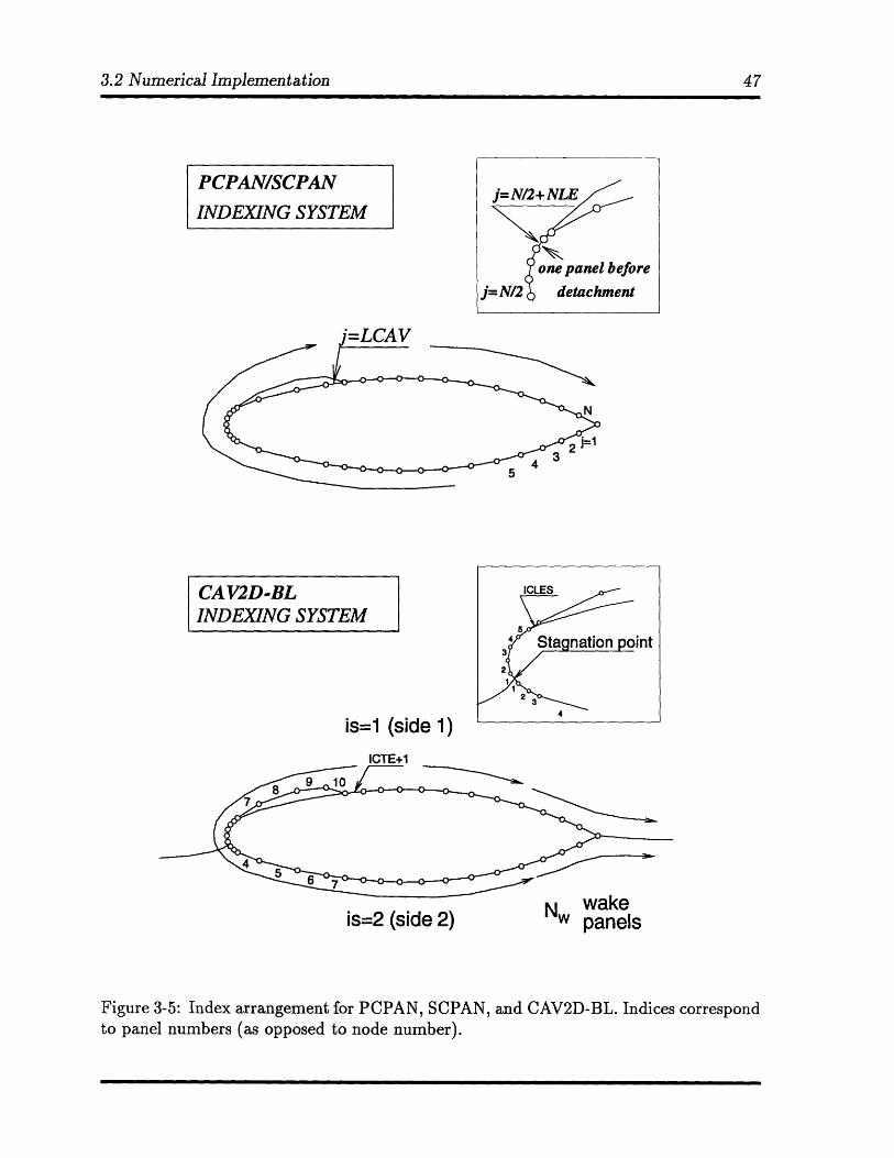
3.2.5 Indexing of the panels
In coupling PCPAN and CAV2D-BL, careful steps must be taken in defining the regions
where the boundary conditions are to be applied. The systems used in indexing the
panels are defined differently in PCPAN than in CAV2D-BL as shown in Figure 3-5. In
PCPAN, the panels are numbered clockwise, where the first index is at the trailing edge
3.2 Numerical Implementation 46
of the foil.
On the other hand, CAV2D-BL first searches for the stagnation point. The location
of the stagnation point is placed in the center of the panel. On the suction side, the first
index is the half-panel above the stagnation point; subsequent numbers follow clockwise.
On the pressure side, the first index is the half-panel below the stagnation point; sub-
sequent numbers follow counter-clockwise, as shown in Figure 3-5. In CAV2D-BL, the
suction side of the foil is called side 1 (is=l) and the pressure side of the foil is side 2
(is=2).
The following quantities are used to specify the cavity location:
* NLE - number of panels between leading edge and cavity detachment (PCPAN)
* LCAV - cavity trailing edge node number (PCPAN)
* IBL - panel number index (CAV2D-BL)
* ICLES - cavity leading edge panel number, suction side (CAV2D-BL)
* ICLEP - cavity leading edge panel number, pressure side (CAV2D-BL)
* ICTE - cavity trailing edge panel number (CAV2D-BL)
These values are used to specify panels on which Cf must go to zero. Notice that the
values given from PCPAN refer to the panel nodes while the values from CAV2D-BL
refer to the actual panel and are related to NLE and LCAV given from PCPAN in the
following manner.
The indices in PCPAN are related to those in CAV2D-BL by:
IBL = j (3.37)
ICLES = NLE + 1
ICTE = LCAV- N/2 +1
3.2 Numerical Implementation
PCPAN/SCPANINDEXING SYSTEM
CAV2D-BLINDEXING SYSTEM
is=1 (side 1)ICTE+1
is=2 (side 2) Nw panelspanels
Figure 3-5: Index arrangement for PCPAN, SCPAN, and CAV2D-BL. Indices correspondto panel numbers (as opposed to node number).
re
I. I
I 1
j--
3.3 Analytical Forces
For side 1:
nonzero 1 < j < ICLES
0 ICLES < j < ICTECf = (3.38)
nonzero ICTE < j• N/2 + NSTAG
0 j > N/2 + NSTAG
For side 2:
i nonzero 1 < j < N/2 - NSTAG0 j > N/2 - NSTAG (3.39)
where N is the number of panels representing the compound foil and cavity surface,
NF is the number of panels on the pressure side of the foil surface, and NSTAG is the
number of panels shifted from the centerline of the leading edge.
3.3 Analytical Forces
The lift coefficient, corresponding to the coordinate system shown in Figure 3-2, is com-
puted by taking the vertical component of the pressures integrated over the entire foil
surface. This expression is given by:
CL= • C nds (3.40)
where C•p are the "viscous" pressures, or the pressures computed on the displaced foil
surface as shown in Figure 3-7, and n, is the y-component of the unit normal vector.
The drag is composed of an inviscid and viscid contribution as such:
CD = Cn + C (3.41)
The inviscid term, C1Dv, is attributed to the drag of the cavity and is given by:
CP= JC)vnxds (3.42)
3.4 Convergence Characteristics
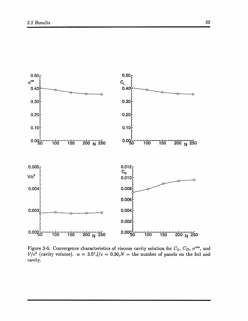
where Cr" are the inviscid pressures shown in Figure 3-7 and n, is the x-component of
the unit normal vector. Cavity drag can be explained by attenuation of pressure near
the trailing edge of the cavity, accurately modeled by the pressure recovery termination
model, equation (3.7).
CyZ8 is the viscous drag term and is given by the "far-wake" approximation as (Drela,
1989):
CDP = -(3.43)c
where 0, is the momentum thickness computed far downstream,3 as shown in Figure
3-2.
3.4 Convergence Characteristics
For 200 panels on a HP 9000/735 with a risc chip, the coupled PCPAN/CAV2D-BL took
less than two minutes.
The convergence of the results of the viscous cavity solution with number of panels
is shown in Figure 3-6. The inviscid solution converges much quicker than the viscous
solution. The viscous cavitation number, a" , is not constant over the extent of the cavity,
evident in Figure 3-7.
3.5 Results
An example of results from this method is shown in Figure 3-7. This shows the case of
a 20% cavity at 3.5 degrees with the boundary displacement thickness superimposed on
the foil and wake surface. Shown at the bottom of Figure 3-7 are the inviscid and viscous
pressure distributions on the foil. Notice that viscosity largely affects the cavitation
number. In addition, the pressure is not constant over the entire extent of the cavity
anymore. From comparing the areas under the viscous and inviscid pressure distributions,
we can also infer that the lift coefficient decreases due to the viscous effects.
3 Five chord lengths aft of the trailing edge.
3.5 Results
I.. . I.3 -'..
100 150 200 N
0.50
CL0.4
0.30
0.20
0.10
An n250
100 150 200 N 250
100 150 200 N
Figure 3-6: Convergence characteristics of viscous cavity solution for CL, CD, a"vi, andV/c' (cavity volume). a = 3.5 0 ,l/c = 0.30,N = the number of panels on the foil andcavity.
0
0.50
evis0.40•
0.30
0.20
0.10
0I0
0.005
V/c2
0.004
0.003
An n
250. -5 %.0
f% f, 4 f
!"50
0.5
Ginviscid
0.5
1.0 xl/
1.0 X/C
Figure 3-7: Above: Present method's predictionViscous and inviscid pressure distribution on foi
of heavy foil with viscous effects. Below:
3.5 Results
Re = 2.68 x 10⁶
a = 3.50Vc = 0.20
0.20
y/c0.10
0.00
-0.10
A0200.0.
1.0
-Cp0.5
0.0
-0.5
-1 n
0
0.0
1.5
1.5
E
1~~~~1~~~~1
3.6 Cavity Detachment Point
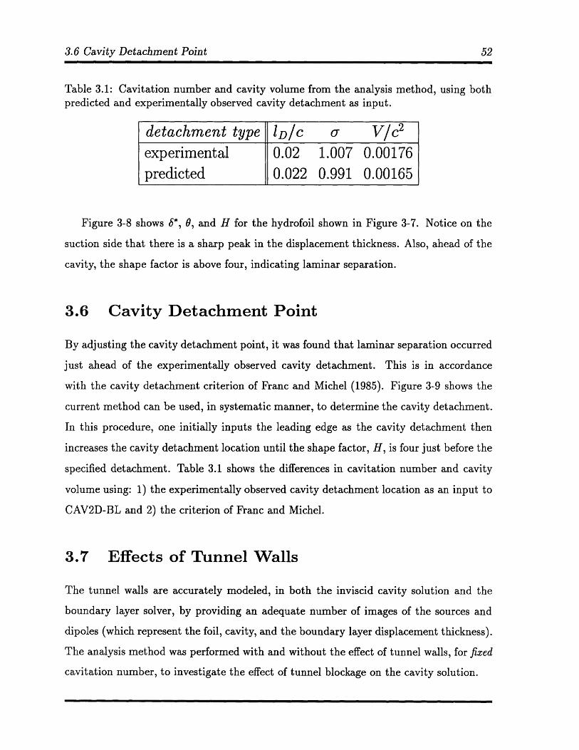
Table 3.1: Cavitation number and cavity volume from the analysis method, using bothpredicted and experimentally observed cavity detachment as input.
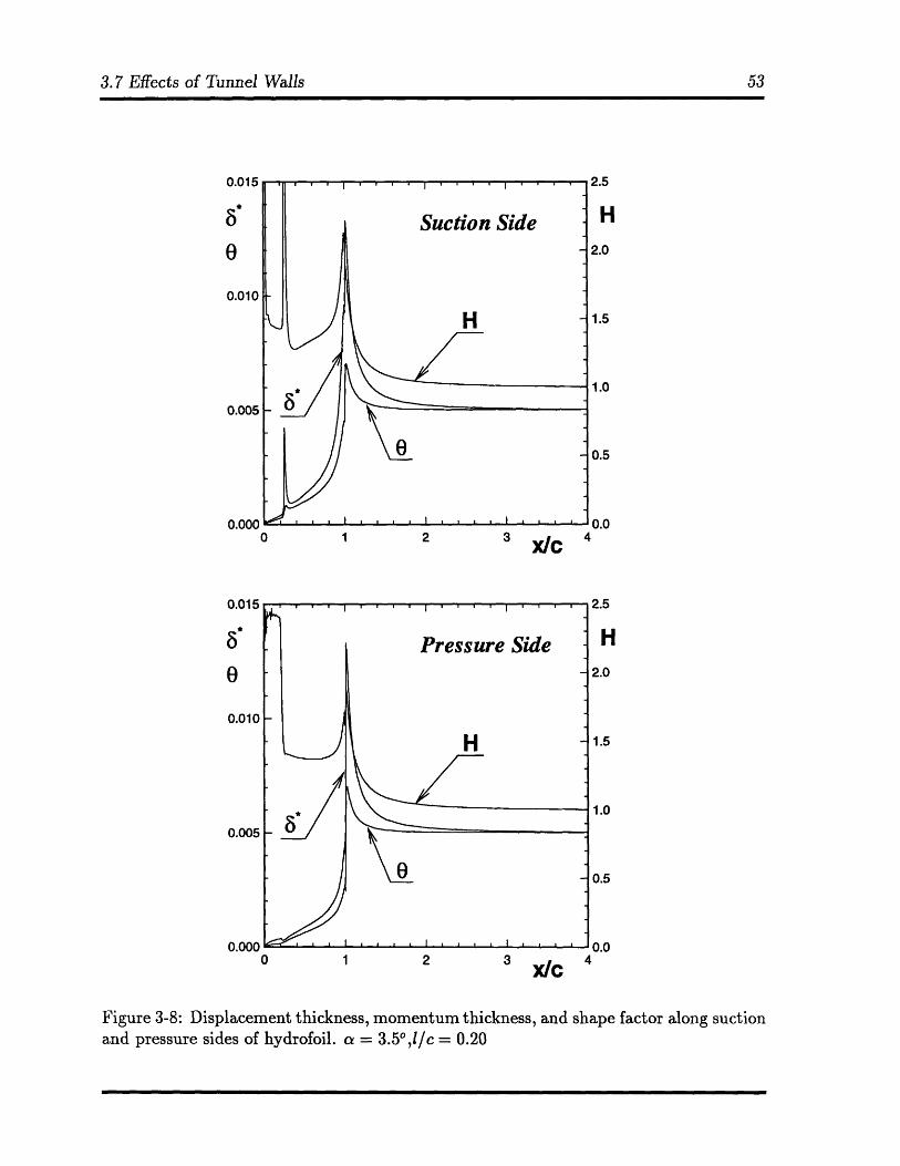
Figure 3-8 shows 6*, 0, and H for the hydrofoil shown in Figure 3-7. Notice on the
suction side that there is a sharp peak in the displacement thickness. Also, ahead of the
cavity, the shape factor is above four, indicating laminar separation.
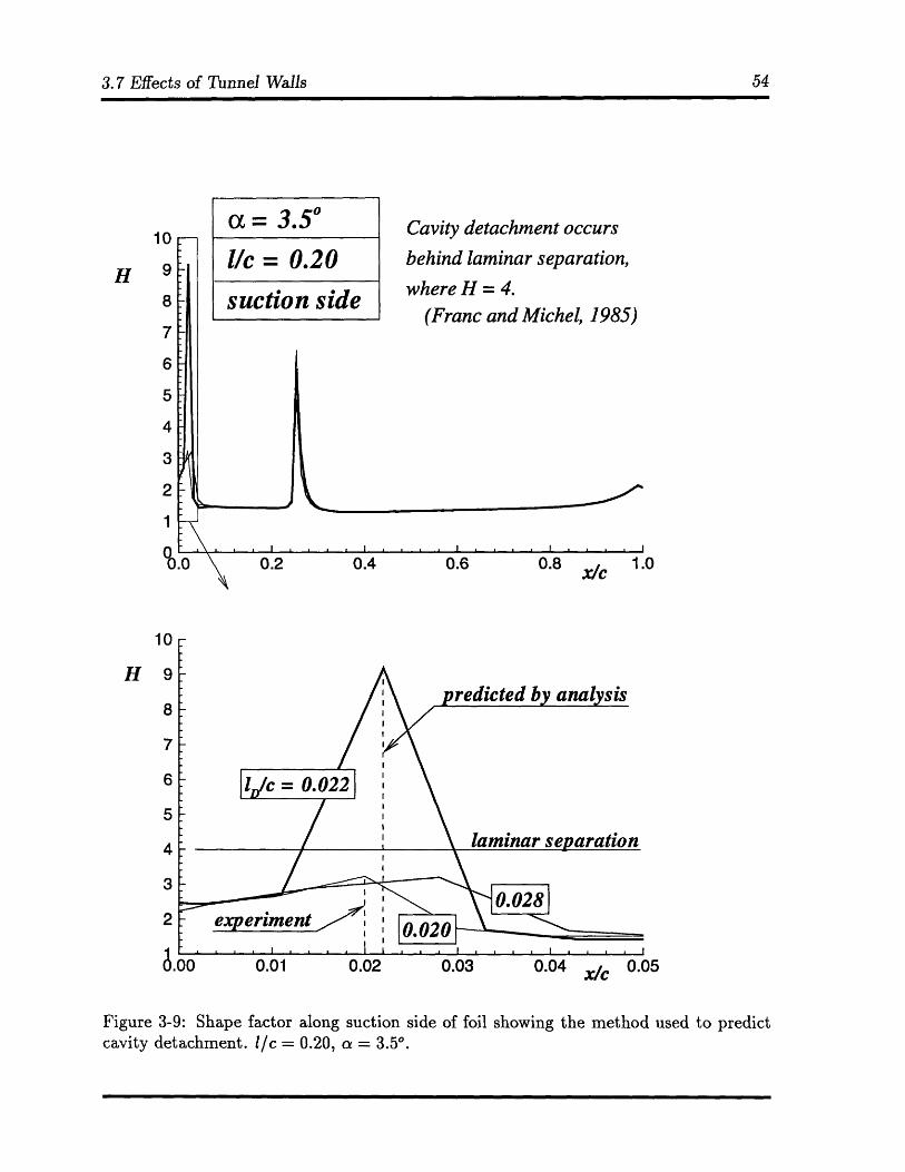
3.6 Cavity Detachment Point
By adjusting the cavity detachment point, it was found that laminar separation occurred
just ahead of the experimentally observed cavity detachment. This is in accordance
with the cavity detachment criterion of Franc and Michel (1985). Figure 3-9 shows the
current method can be used, in systematic manner, to determine the cavity detachment.
In this procedure, one initially inputs the leading edge as the cavity detachment then
increases the cavity detachment location until the shape factor, H, is four just before the
specified detachment. Table 3.1 shows the differences in cavitation number and cavity
volume using: 1) the experimentally observed cavity detachment location as an input to
CAV2D-BL and 2) the criterion of Franc and Michel.
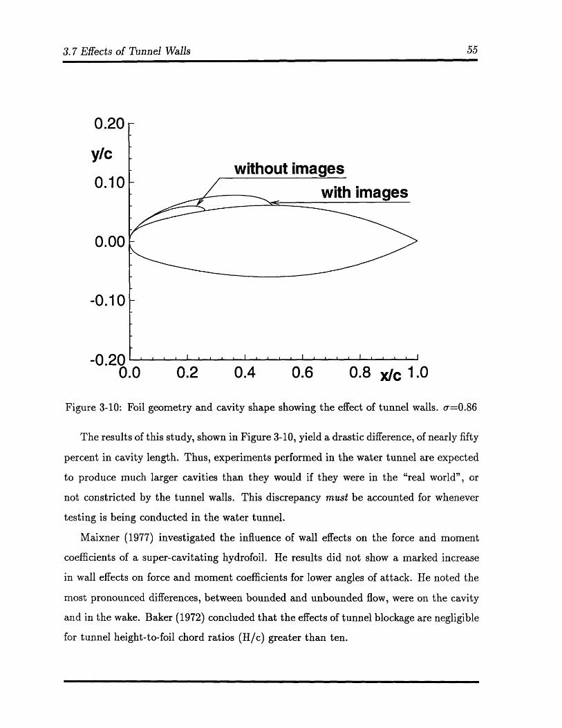
3.7 Effects of Tunnel Walls
The tunnel walls are accurately modeled, in both the inviscid cavity solution and the
boundary layer solver, by providing an adequate number of images of the sources and
dipoles (which represent the foil, cavity, and the boundary layer displacement thickness).
The analysis method was performed with and without the effect of tunnel walls, for fixed
cavitation number, to investigate the effect of tunnel blockage on the cavity solution.
detachment type ID/cC U V/c 2
experimental 0.02 1.007 0.00176predicted 0.022 0.991 0.00165
3.7 Effects of Tunnel Walls
0.015
5"
0.010
0.005
0.000
0.015
5'
0.010
0.005
0.000
1 2 3 x 4
1 2 3 X/C 4
.3
H.0
.5
.0
.5
.0
'.0
H2.0
1.5
1.0
0.5
n
Figure 3-8: Displacement thickness, momentum thickness, and shape factor along suctionand pressure sides of hydrofoil. a = 3.50,1/c = 0.20
,,
V.,
Cavity detachment occurs
I/c = 0.20 behind laminar separation,
suction side where H = 4.(Franc and Michel, 1985)
0.2 0.4 0.6 0.8 x/c
0.01 0.02 0.03 0.04 x/e
1.0
0.05
Figure 3-9: Shape factor along suction side of foil showing the method used to predictcavity detachment. i/c = 0.20, a = 3.50 .
3.7 Effects of Tunnel Walls
K = 3.50
o0.0
'1UH 9
8
7
6
5
4
3
2
I6.00
£'t
3.7 Effects of Tunnel Walls
,~ ~U.4U
y/c0.10
0.00
-0.10
-_n on0.0 0.2 0.4 0.6 0.8 x/c 1.0
Figure 3-10: Foil geometry and cavity shape showing the effect of tunnel walls. cr=0.86
The results of this study, shown in Figure 3-10, yield a drastic difference, of nearly fifty
percent in cavity length. Thus, experiments performed in the water tunnel are expected
to produce much larger cavities than they would if they were in the "real world", or
not constricted by the tunnel walls. This discrepancy must be accounted for whenever
testing is being conducted in the water tunnel.
Maixner (1977) investigated the influence of wall effects on the force and moment
coefficients of a super-cavitating hydrofoil. He results did not show a marked increase
in wall effects on force and moment coefficients for lower angles of attack. He noted the
most pronounced differences, between bounded and unbounded flow, were on the cavity
and in the wake. Baker (1972) concluded that the effects of tunnel blockage are negligible
for tunnel height-to-foil chord ratios (H/c) greater than ten.
Chapter 4
CAV2D-BL: Super-Cavitating
Boundary Layer Solver
4.1 Formulation & Numerical Implementation
4.1.1 Step 1: Calculate cavity height (SCPAN)
The formulation of the super-cavitating hydrofoil is very similar to the that of partial-
cavitation, given in Chapter 3. Figure 4-1 shows a discretized version of a super-cavitating
foil and a definition of the main parameters.
As a first iteration for the non-linear solution, SCPAN uses the cavity shape from
the linear solution. The linear solution is obtained by applying a source and vorticity
formulation.
In a transition region at the trailing edge of the cavity, an end parabola model (as
shown in Figure 4-2) replaces the cavity shape. This model serves to accurately represent
the actual pressure attenuation as evidenced in experiments (Meijer, 1959). The shape
of the end parabola is given by the linear solution. Its vertical position is determined
iteratively until the kinematic boundary condition is satisfied on its surface.
Over the cavity surface, not including the transition region, the dynamic boundary
condition is applied. In the transition region, the kinematic boundary condition is ap-
plied. The cavity shape is updated iteratively until the kinematic boundary condition is
4.1 Formulation & Numerical Implementation
y
Figure 4-1: Super-cavitating hydrofoil in inviscid non-linear theory. Definition of mainparameters. Panel arrangement on the cavity and foil shown for N = 80.
X- C
a3n
n
Figure 4-2: The super-cavitating end parabola modelcondition is applied.
where the kinematic boundary
4.2 Indexing of the panels
I
Figure 4-3: Super-cavitating hydrofoil with its boundary displacement thickness.
satisfied over the entire cavity extent.
4.1.2 Steps 2 & 3: Solve viscous flow around "compound" foil
(CAV2D-BL)
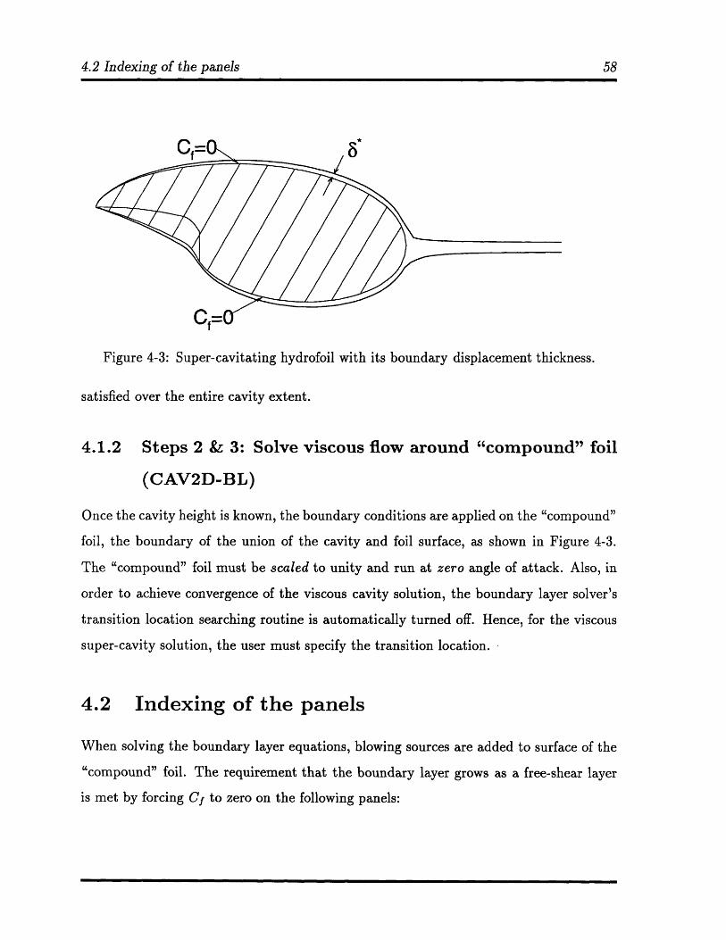
Once the cavity height is known, the boundary conditions are applied on the "compound"
foil, the boundary of the union of the cavity and foil surface, as shown in Figure 4-3.
The "compound" foil must be scaled to unity and run at zero angle of attack. Also, in
order to achieve convergence of the viscous cavity solution, the boundary layer solver's
transition location searching routine is automatically turned off. Hence, for the viscous
super-cavity solution, the user must specify the transition location.
4.2 Indexing of the panels
When solving the boundary layer equations, blowing sources are added to surface of the
"compound" foil. The requirement that the boundary layer grows as a free-shear layer
is met by forcing Cf to zero on the following panels:
4.3 Results
* For side 1 (is=l):
Cf=0 j>0 (4.1)
* For side 2 (is=2):
nonzero j < ICLEP0 j > ICLEP (4.2)
* where SCPAN is related to CAV2D-BL by:
ICTE = N/2 + 1 (4.3)
ICLES = 0
ICLEP = NF+1
and NF is the number of panels representing the pressure side of the foil surface
4.3 Results
The present method is applied to a super-cavitating foil with NACA 4-digit camber
distribution and linear thickness form. Figure 4-4 shows the resulting nonlinear cavity
shape and displacement thickness along the foil for a Reynolds number of 2 x 10⁷. Notice
that viscosity has little effect on the pressure distribution in Figure 4-4. Also shown in
Figure 4-4 is the friction coefficient on the pressure side of foil and cavity, which is forced
to zero aft of the trailing edge of the foil.
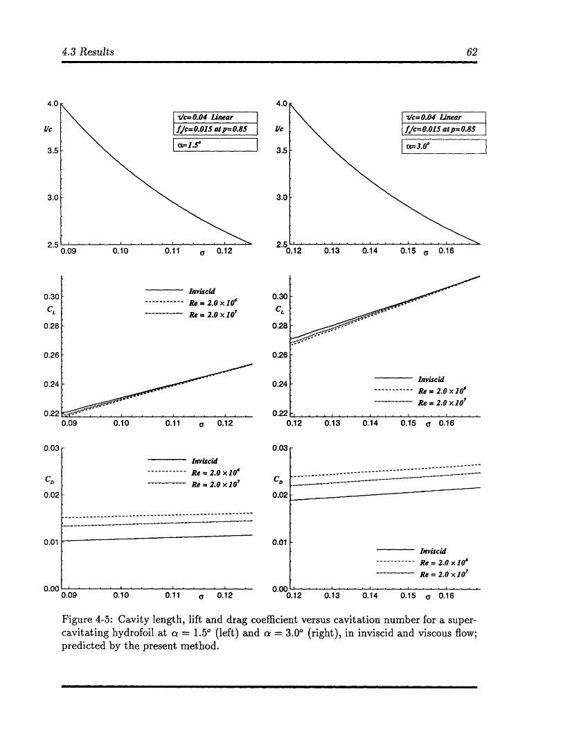
Figure 4-5 shows lift and drag characteristics for various cavitation numbers. It is
evident in this figure that viscosity has a negligible effect on the lift. As the cavitation
number increases, the viscous lift increases with respect to the inviscid lift. The reason for
this is that the displacement thickness grows with increasing cavitation number, changing
the effective angle of attack of the "compound" foil. The difference in drag coefficients,
between inviscid and viscous flow, is much more pronounced, as shown in Figure 4-5.
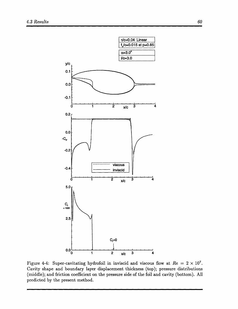
4.3 Results
r/c=0.04 Linearfjc=0.015 at p=0.85
l(=3.00I/c=3.0
- . . ! . .
2 x/c 3
--------- viscousinviscid
2 3
C,=O
Figure 4-4: Super-cavitating hydrofoil in inviscid and viscous flow at Re = 2 x 10'.Cavity shape and boundary layer displacement thickness (top); pressure distributions(middle); and friction coefficient on the pressure side of the foil and cavity (bottom). Allpredicted by the present method.
y/c
0.1
0.0
-0.1
0.0
-C,
-0.2
-0.4
xl
· · _··__·___··__~~_~ .
-U.
,,
--
4.3 Results
Table 4.1: Convergence of viscous cavity solution (a, V/c2 , CL and CD) with number ofpanels. Super-cavitating hydrofoil; r/c = 0.045, fo/c = 0.015, p = 0.85, a = 3 .
N a V/c2 CL CD100 0.145 0.365 0.282 0.0219160 0.146 0.364 0.287 0.0223200 0.146 0.363 0.292 0.0231
This difference is largely attributed to the frictional drag on the pressure side of the foil.
Figure 4-5 can be used to determine an "equivalent" cavity length which, if run under
inviscid flow, would produce the same lift and cavity volume as the viscous cavity solution.
Notice that the inviscid cavity solution underpredicts the cavity length for given CL and
a. This can be reasoned by intuition in the following way: the angle of attack in viscous
flow would have to be increased to produce the larger cavity that inviscid flow predicts;
therefore, if the same angle of attack were used in both inviscid and viscous theory, the
inviscid solution must produce a smaller cavity. Different cavity lengths for a and a,
are shown in Kinnas et al (1994) for inviscid flow and various Reynolds numbers. The
"equivalent" a concept can be applied to three dimensional geometries in a strip-wise
sense. This is addressed much more extensively in Section 6.1.
Table 4.1 shows the convergence characteristics of the viscous super-cavitating solu-
tion for increasing panels numbers.
4.3 Results
7/c= 0.04 Linearfjc= 0.015 atp=0.85
Z .. . . i3.5
3.0
4.0
i/c
3.5
3.0
2.50.12 0.13 0.14 0.15 , 0.16
Inviscid
Re = 2.0 x 10l
Re = 2.0 x 10'
0.30
CL
0.28
0.26
0.24
0.220.11 a 0.12
Inviscid---------- Re = 2.0 x 10'...................-. Re = 2.0 x 10'
U.UO
CD
0.02
0.01
An0.11 a 0.12
0
0.12
0.12
0.13 0.14 0.15 a 0.16
0.13 0.14 0.15 a 0.16
Figure 4-5: Cavity length, lift and drag coefficient versus cavitation number for a super-cavitating hydrofoil at a = 1.50 (left) and a = 3.00 (right), in inviscid and viscous flow;predicted by the present method.
0.11 a 0.12
T/c=0.04 Linear
fc=0.015OI atp=0.85
xa=3.0"
la).
I]7
0.09 0.10
0.09 0.10
0.30
CL0.28
0.26
0.24
0.22
V.V
D0.02
0.02
0.01
0.00
Inviscid
---------- Re = 2.0 x 10l-..................... Re = 2.0 x10⁷
0.09 0.10
Inviscid---------- Re = 2.0 x 10 6
Re = 2.0 x 10 7
2 r
,-;-- ........... ........~ ' ~ ~ '
. . . . . . . . |' |= | | . I I I I I ,I I
5-
-----------
E
-·
n nnr
rr ~n
p
-------------------------------------------
--- -------- ---- -----
E
I .

Chapter 5
Experimental Versus Numerical
Results: Phases II & III
This section contains experimental versus numerical comparisons, from Phases I and II
of the experiment, for the quantities: velocities along contour surrounding the hydrofoil,
velocities in boundary layer region, velocities near cavity surface, pressure measurements,
and forces acting on the hydrofoil. Correlations between experiment and theory were also
made with the data from Phase I of the experiment; they are given in Appendix D.
The angles of attack shown in the figures of this section may be confusing. With
each reinstallation of the foil, the angle of attack changed slightly. All of the boundary
layer measurements and measurements along the rectangular contour 1 were performed
in Phase II of the experiment, where the angle of attack was 3.50. All of the pressure
measurements and velocity measurements near the cavity surface were performed in the
third phase of the experiment, where the angle of attack was 3.250. Refer to Table 2.1
for the details of each phase of the experiment.
The underlying intention for these comparisons is to be extremely systematic in cor-
relating the analytical results with the experimental data. The comparisons between
experiment and theory, in the case of cavitating flow, are based on the assumption that
1Except for the fully-wetted case, which was performed in Phase III. This measurement was performedagain in Phase III because the free-stream velocity for the fully-wetted case in Phase II was inaccuratelyrecorded.
5.1 Forces in the Experiment
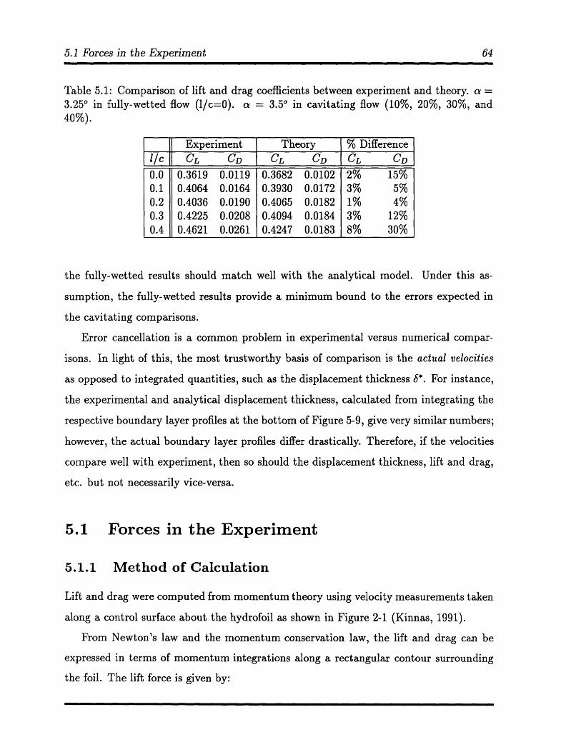
Table 5.1: Comparison of lift and drag coefficients between experiment and theory. a =3.250 in fully-wetted flow (l/c=0). a = 3.50 in cavitating flow (10%, 20%, 30%, and40%).
the fully-wetted results should match well with the analytical model. Under this as-
sumption, the fully-wetted results provide a minimum bound to the errors expected in
the cavitating comparisons.
Error cancellation is a common problem in experimental versus numerical compar-
isons. In light of this, the most trustworthy basis of comparison is the actual velocities
as opposed to integrated quantities, such as the displacement thickness 5*. For instance,
the experimental and analytical displacement thickness, calculated from integrating the
respective boundary layer profiles at the bottom of Figure 5-9, give very similar numbers;
however, the actual boundary layer profiles differ drastically. Therefore, if the velocities
compare well with experiment, then so should the displacement thickness, lift and drag,
etc. but not necessarily vice-versa.
5.1 Forces in the Experiment
5.1.1 Method of Calculation
Lift and drag were computed from momentum theory using velocity measurements taken
along a control surface about the hydrofoil as shown in Figure 2-1 (Kinnas, 1991).
From Newton's law and the momentum conservation law, the lift and drag can be
expressed in terms of momentum integrations along a rectangular contour surrounding
the foil. The lift force is given by:
Experiment Theory % Difference1/c CL CD CL CD0.0 0.3619 0.0119 0.3682 0.0102 2% 15%0.1 0.4064 0.0164 0.3930 0.0172 3% 5%0.2 0.4036 0.0190 0.4065 0.0182 1% 4%0.3 0.4225 0.0208 0.4094 0.0184 3% 12%0.4 0.4621 0.0261 0.4247 0.0183 8% 30%
5.1 Forces in the Experiment
L = ML + MPB - M - M!T + PZ (5.1)
where M is the momentum flux through the left, L, right, R, bottom, B, and top, T
sides of a rectangular contour about a hydrofoil (see Figure 2-1) and are defined as:
MLR = WL,RUL,RdzZB
M 'B,T = P WB,TWB,Tdx (5.2)
PZ = 2( + w 2 2 )dx (5.3)
and,
/z U /
z U
D = pU Aundz - pZ (Au) 2 dz (5.4)JzL JZL
where AuR is the horizontal velocity defect in the wake and ZL and zu is the vertical
location of the bottom and top of the wake defect region, respectively, of the rectangular
contour.
Thus, the data collected from a contour around the foil can be used with these inte-
grations to calculate the lift and drag force acting on the foil. In this formulation, the
flow is considered inviscid on the top and bottom cuts of the contour. Also, the effects
of viscosity due to right and left sides of the rectangle are shown, in Kinnas (1991), to
have negligible effect on the lift.
5.1.2 Comparisons with Theory
Figure 5-1 illustrates the experimental and analytical lift and drag coefficients, computed
from equations (5.1) and (5.4) respectively. In Figure 5-1, the fully-wetted results (1/c=O)
compare very well with the analytical model. For the larger cavity lengths, the experiment
separates from theory. As mentioned earlier, this can be explained by the increased
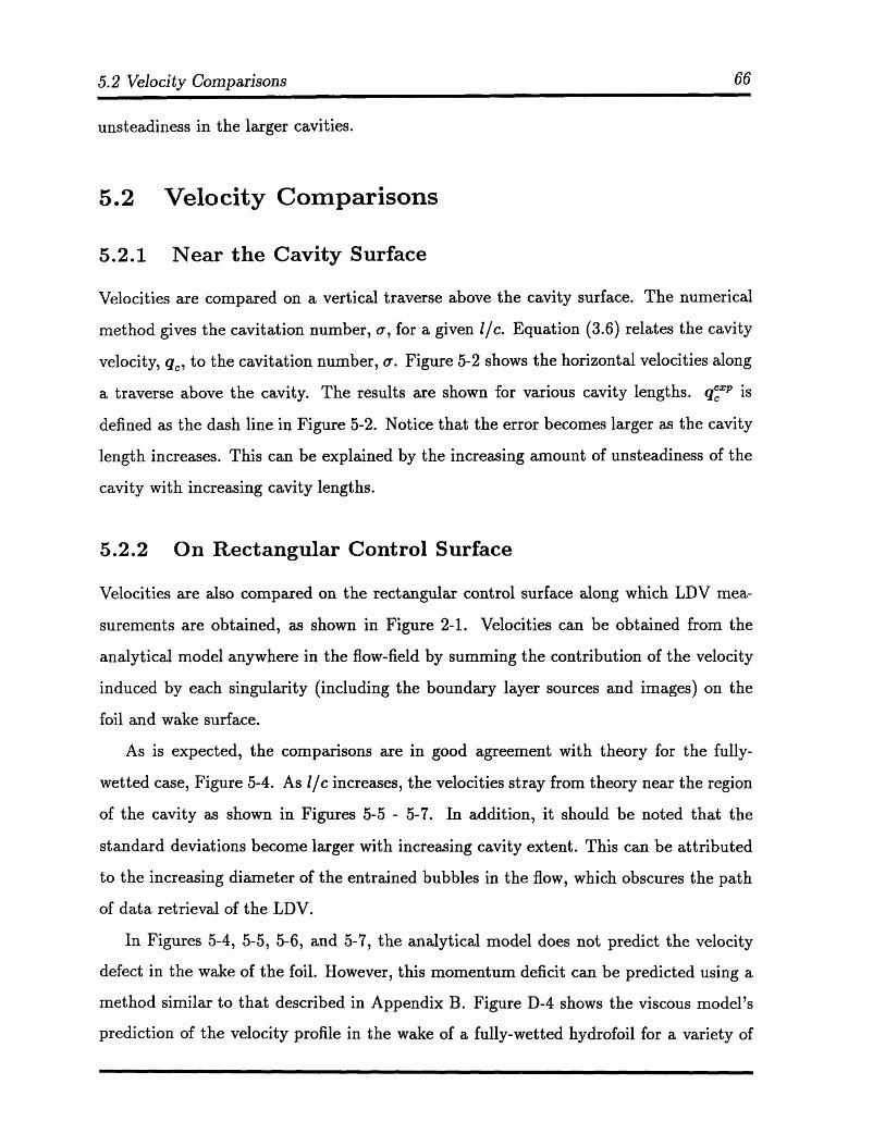
5.2 Velocity Comparisons
unsteadiness in the larger cavities.
5.2 Velocity Comparisons
5.2.1 Near the Cavity Surface
Velocities are compared on a vertical traverse above the cavity surface. The numerical
method gives the cavitation number, o, for a given i/c. Equation (3.6) relates the cavity
velocity, qc, to the cavitation number, a. Figure 5-2 shows the horizontal velocities along
a traverse above the cavity. The results are shown for various cavity lengths. q "P is
defined as the dash line in Figure 5-2. Notice that the error becomes larger as the cavity
length increases. This can be explained by the increasing amount of unsteadiness of the
cavity with increasing cavity lengths.
5.2.2 On Rectangular Control Surface
Velocities are also compared on the rectangular control surface along which LDV mea-
surements are obtained, as shown in Figure 2-1. Velocities can be obtained from the
analytical model anywhere in the flow-field by summing the contribution of the velocity
induced by each singularity (including the boundary layer sources and images) on the
foil and wake surface.
As is expected, the comparisons are in good agreement with theory for the fully-
wetted case, Figure 5-4. As 1/c increases, the velocities stray from theory near the region
of the cavity as shown in Figures 5-5 - 5-7. In addition, it should be noted that the
standard deviations become larger with increasing cavity extent. This can be attributed
to the increasing diameter of the entrained bubbles in the flow, which obscures the path
of data retrieval of the LDV.
In Figures 5-4, 5-5, 5-6, and 5-7, the analytical model does not predict the velocity
defect in the wake of the foil. However, this momentum deficit can be predicted using a
method similar to that described in Appendix B. Figure D-4 shows the viscous model's
prediction of the velocity profile in the wake of a fully-wetted hydrofoil for a variety of
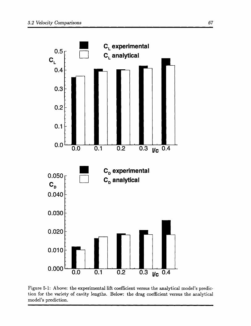
5.2 Velocity Comparisons
LI0.5CL
0.4
0.3
0.2
0.1
0.0
0.050CD
0.040
0.030
0.020
0.010
0.000
CL
CL
m-
0.1
CDFZ CD
experimentalanalytical
0.2
I-
0.3 Vc 0.4
experimentalanalytical
0.0 0.1 0.2 0.3 Vc 0.4
Figure 5-1: Above: the experimental lift coefficient versus the analytical model's predic-tion for the variety of cavity lengths. Below: the drag coefficient versus the analyticalmodel's prediction.
0.0_ __
m
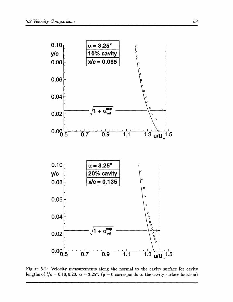
I I0.10y/c0.08
0.06
0.04
0.02
0.00 0.7%I vD
I l-n I
o
o
(o
o0oo0
O
0.7 0.9 1.1
Figure 5-2: Velocity measurements along the normal to the cavity surface for cavitylengths of i/c = 0.10, 0.20. a = 3.250. (y = 0 corresponds to the cavity surface location)
5.2 Velocity Comparisons
0
.1U. IU
y/c0.08
0.06
0.04
0.02
n n1.3 uIU 1.5'"0.5
00
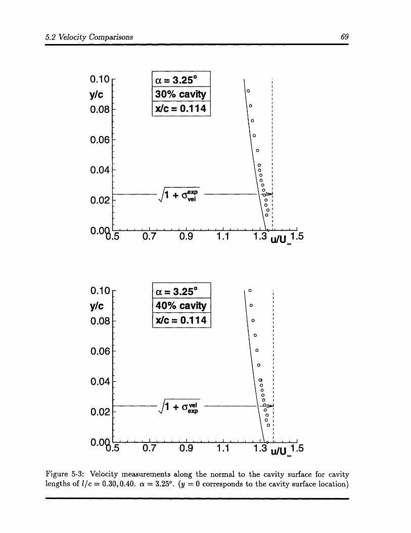
5.2 Velocity Comparisons
a = 3.25030% cavityx/c = 0.114
U. Iu
y/c0.08
0.06
0.04
0.02
n n0.7 0.9
I I
4
x/
0.7
1.1
o
o
o
o
o
ooooo
0Oi0'
0'0
o Iooo-ODi0
1.3 u/U 1.5
= 3.25
D% cavity o
c= 0.114 o
o
o
Ooo
1 +vetoexp 0o
OiOI
, , , I . . I . .. .
0.9 1.1 1.3 ulU 1.5
Figure 5-3: Velocity measurements along the normal to the cavity surface for cavitylengths of 1/c = 0.30,0.40. a = 3.25'. (y = 0 corresponds to the cavity surface location)
ft .4 rl
c
0.10
y/c0.08
0.06
0.04
0.02
n nn". 6.
.1
I i i . . . . . . . . . . . . . . . . . • .. . . .
. . . . . . . . . . . . . • -- . , ,
1+ expvel
. ,10.5
,/
5
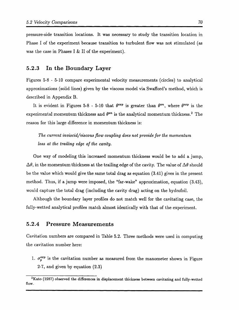
5.2 Velocity Comparisons
pressure-side transition locations. It was necessary to study the transition location in
Phase I of the experiment because transition to turbulent flow was not stimulated (as
was the case in Phases I & II of the experiment).
5.2.3 In the Boundary Layer
Figures 5-8 - 5-10 compare experimental velocity measurements (circles) to analytical
approximations (solid lines) given by the viscous model via Swafford's method, which is
described in Appendix B.
It is evident in Figures 5-8 - 5-10 that 0e"P is greater than "an, where 0e" p is the
experimental momentum thickness and 0 a8 is the analytical momentum thickness.2 The
reason for this large difference in momentum thickness is:
The current inviscid/viscous flow coupling does not provide for the momentum
loss at the trailing edge of the cavity.
One way of modeling this increased momentum thickness would be to add a jump,
AO, in the momentum thickness at the trailing edge of the cavity. The value of AO should
be the value which would give the same total drag as equation (3.41) gives in the present
method. Thus, if a jump were imposed, the "far-wake" approximation, equation (3.43),
would capture the total drag (including the cavity drag) acting on the hydrofoil.
Although the boundary layer profiles do not match well for the cavitating case, the
fully-wetted analytical profiles match almost identically with that of the experiment.
5.2.4 Pressure Measurements
Cavitation numbers are compared in Table 5.2. Three methods were used in computing
the cavitation number here:
1. orp" is the cavitation number as measured from the manometer shown in Figure
2-7, and given by equation (2.3)
2 Kato (1987) observed the differences in displacement thickness between cavitating and fully-wettedflow.
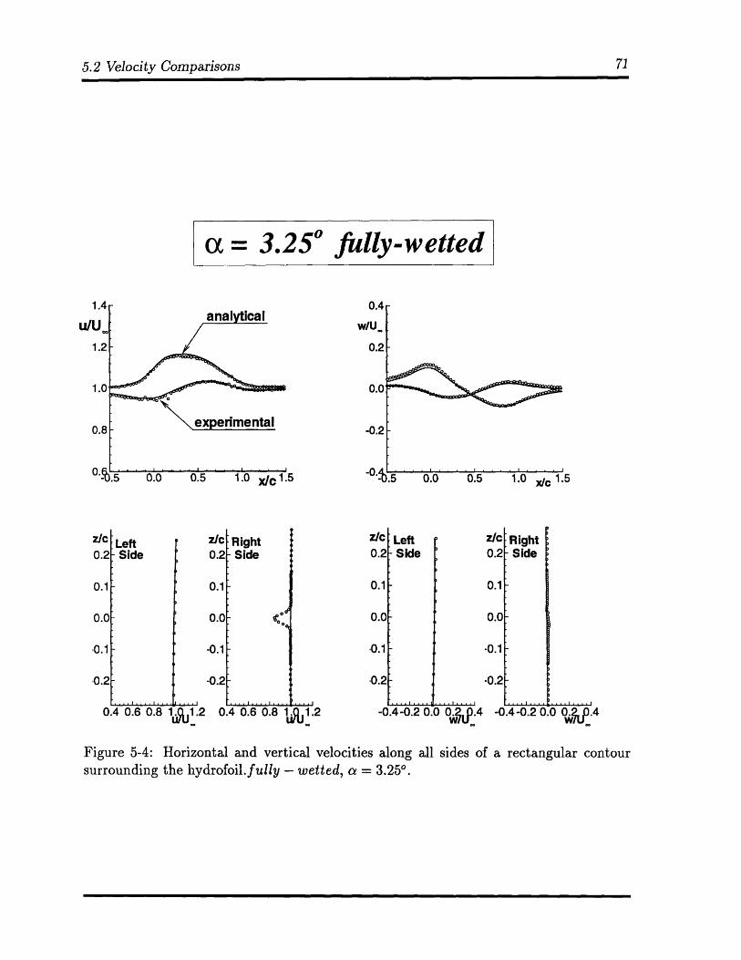
5.2 Velocity Comparisons
a = 3.250 fully-wetted
0.0 0.5 1.0 x/ 1.5
LeftSide
0.4 0.6 0.8 lOu1 .2
RightSide
Z/C0.2
0.4 0.6 0.8 1.u•%1.2tk%1.
LeftSide
.... I ....
z0
0
0
.0
-0).1
-0.4-0.2 0.0 O &.4
(C
.2
.1
.0
.1
.2
: Right-Side
i
-0.4-0.2 0.0 093 .4
Figure 5-4: Horizontal and vertical velocities along all sides of a rectangular contoursurrounding the hydrofoil.fully - wetted, a = 3.250.
U.4
w/U,
0.2
-0.2
,,r
E
E
Ii , , I .. .. I , , , I . . . .I ,., I ..., . I .... .... I .... I .... i
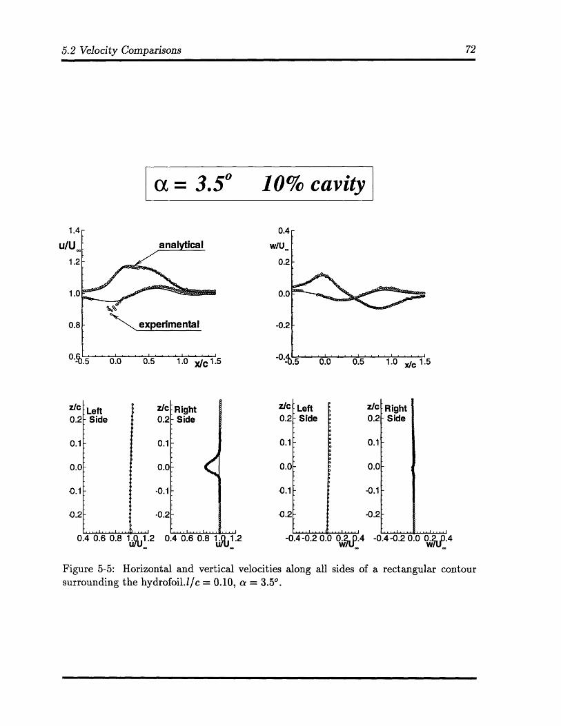
5.2 Velocity Comparisons
S= 3.50 10% cavity
.1
.2
0.4
w/U
0.2
LeftSide
-0.1
-0.2
0.4 0.6 0.8 IuO1 .2
RightSide
-0.2
0.4 0.6 0.8 1.iu%1.2
0.0 0.5 1.0 xc 1.5
Left-Side
-
zlc0.2
0.1
0.0
-0.1
-0.2
-0.4-0.2 0.0 0o .4
Right- Side
-0.4-0.2 0.0 0.V.4
Figure 5-5: Horizontal and vertical velocities along all sides of a rectangular contoursurrounding the hydrofoil.1/c = 0.10, a = 3.50 .
U)
.0.
'0.
4 A
-
.I....I....I....I
-
-
-
.. ,.. I .... ! ,.. .. . . . . .. .. I . ... . . . . I . . . . I
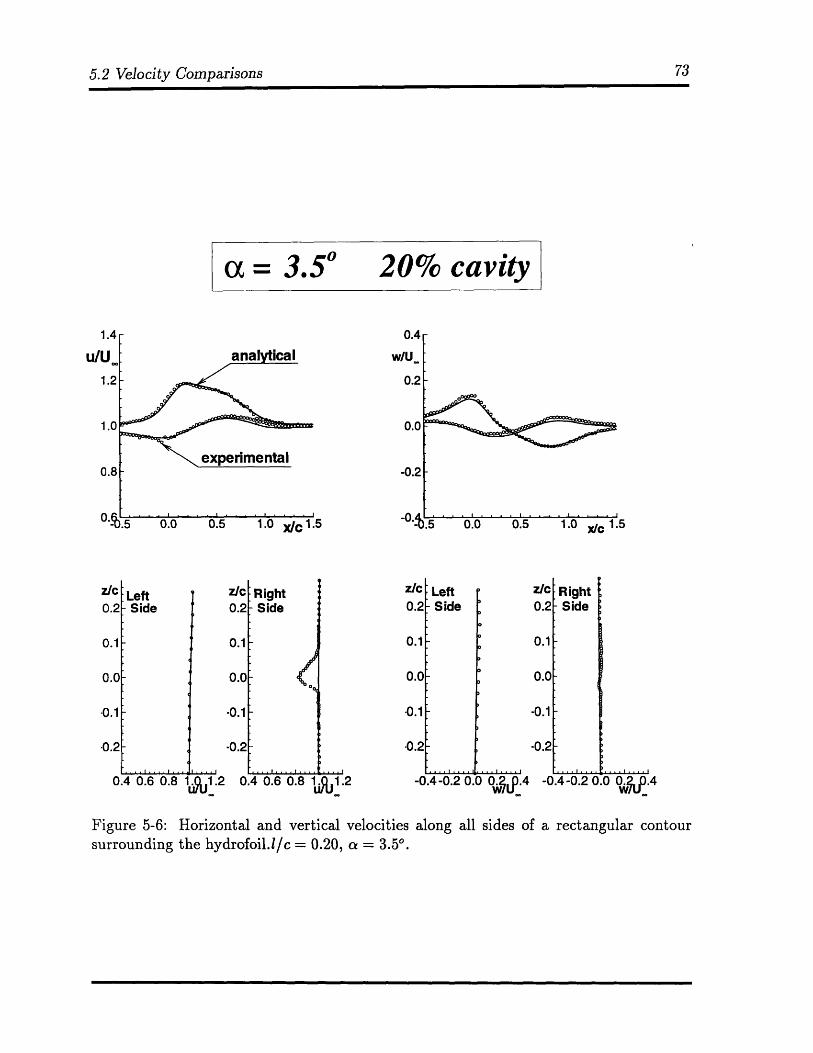
5.2 Velocity Comparisons
a = 3.50 20% cavity
U.4
0.2
-0.2
0 A
! Side
t i
11- I
.1-
0.4 0.6 0.8 1U%1.2
0.0 0.5 1.0 xc 1.5
LeftSide
I-
I-
EE
-0.4-0.2 0.0 O0 .4 -0.4-0.2 0.0
Figure 5-6: Horizontal and vertical velocities along all sides of a rectangular contoursurrounding the hydrofoil.1/c = 0.20, a = 3.50
U/
,,
-w/U
I .... I.... i .
-·-·.-,
-'-0.5
LefI P
i nt ~··tt f
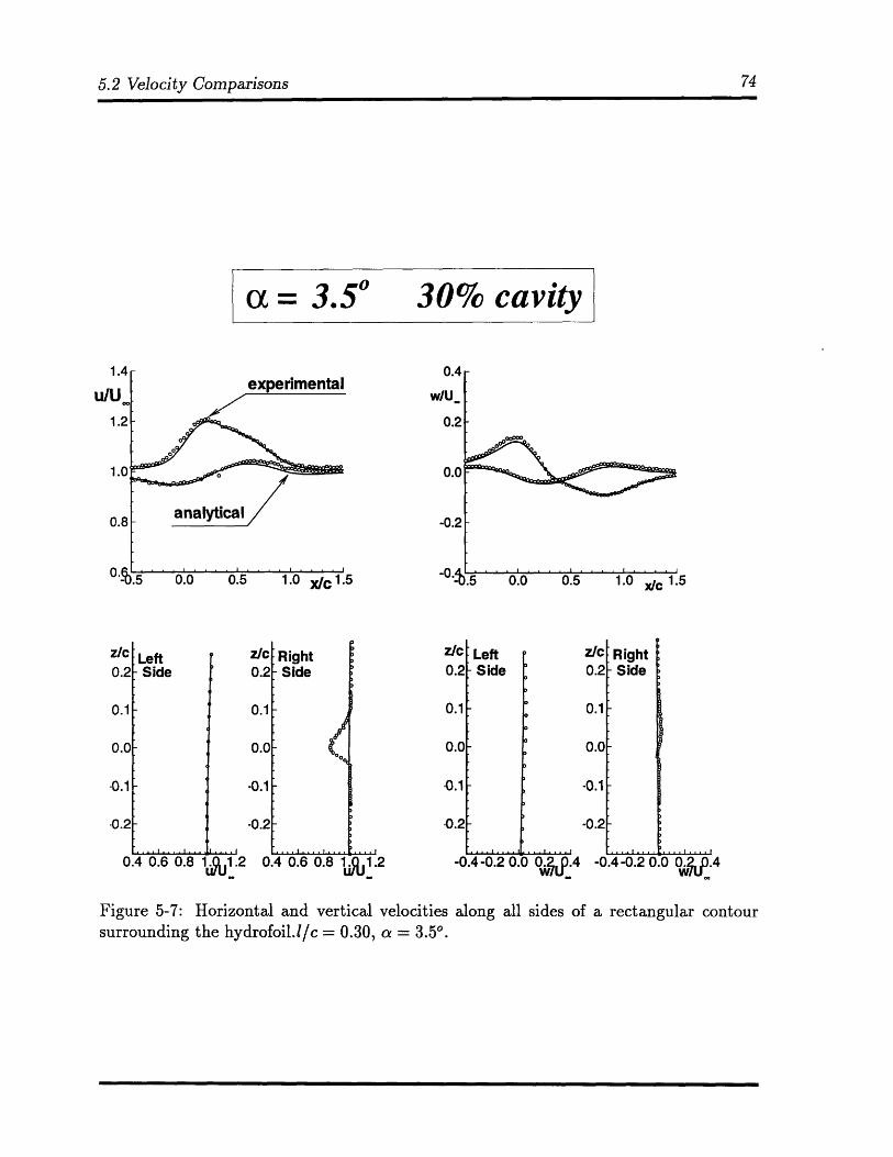
5.2 Velocity Comparisons
a = 3.50 30% cavity
0.0 0.5 1.0 xc 1.5
0.
"0
.1
.2
Left- Side
z/l0.2
-0.1
-0.2
I, I.
0.4 0.6 0.8 1./1 .2
Figure 5-7:
RightSide
6p
z/c0.2
0.1
0.0
.0.1
0.2
0.4 0.6 0.8 1.u%1 .2
Left- Side
-0.4-0.2 0.0 Ow 4
Horizontal and vertical velocities along all sides of a rectangular contoursurrounding the hydrofoil.l/c = 0.30, a = 3.5' .
u/U.4Q
w/U
0.2
-0.2
_f A
,,-
-
.I....I....I1-0..5
I ,t.,I,,,,! ,.. I ... II
'''ll. . . . I . . . . I . . . . .... I
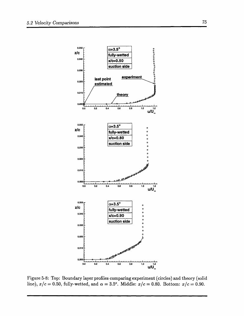
5.2 Velocity Comparisons 75
I ^ I
z/c0.040
0.030
0.020
0.010
0.000
(x=3.50 o0o
0fully-wetted 00x/c=0.50 0suction side 0
00o
ast point experiment 0last point 0
estimated
theory
. .I . . . .I I . . . .
0.0 0.2 0.4 0.6 0.8 1.0 1.2
u/U
z/c0.040
0.030
0.020
0.010
0.000,
a=3.5 o0
fully-wetted 0
x/c=0.80 0
suction side o
0o
-0o
W0
0.0 0.2 0.4 0.6 0.8 1.0 1.2
u/U
U.UDU
z/c
0.040
0.030
0.020
0.010
0.000,
-f=3.5*
o
fully-wetted 00
x/c=0.90 00suction side 00o
0
o
-0 oo
, , l , , , I . .I . . . . ... I , , , i i i
0.0 0.2 0.4 0.6 0.8 1.0 1.2
u/U
Figure 5-8: Top: Boundary layer profiles comparing experiment (circles) and theory (solidline), x/c = 0.50, fully-wetted, and a = 3.50 . Middle: x/ec = 0.80. Bottom: z/c = 0.90.
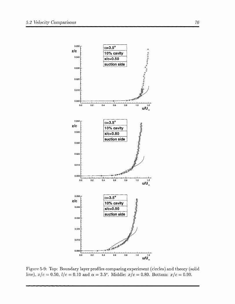
5.2 Velocity Comparisons 76
cc=3.50 o
10% cavity 0o
x/c=0.50 0ooosuction side 00
ooo
oo
o-o
= o
0.0 0.2 0.4 0.6 0.8 1.0 1.2
u/U
(x=3.50
10% cavityx/c=0.80suction side
- i . . . . . .
0.0 0.2 0.4 0.6 0.8 1.0 1.2
u/U
0.050
z/c
0.040
0.030
0.020
0.010
0.000,
0.0 0.2 0.4 0.6 0.8 1.0 12
u/U
Figure 5-9: Top: Boundary layer profiles comparing experiment (circles) and theory (solidline), x/c = 0.50, 1/c = 0.10 and a = 3.50. Middle: x/c = 0.80. Bottom: z/c = 0.90.
0.050
z/c
0.040
0.030
0.020
0.010
0.000
0.050
z/c
0.040
0.030
0.020
0.010
0.000(
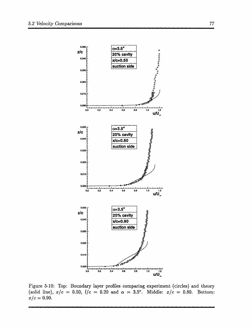
5.2 Velocity Comparisons
ca=3.5 °
20% cavityx/c=0.50suction side
0.050
z/c
0.040
0.030
0.020
0.010
02 0.4 0.6 0.8 1.0 12
uUA
a=3.5°20% cavityx/c=0.80suction side-•
. . . i . . . . i . .-. .
0.2 0.4 0.6 0.8 1.0 1.2
U/U
0.0 0.2 0.4 0.6 0.8 1.0 12
u/U
Figure 5-10: Top: Boundary
(solid line), x/c = 0.50, 1/cx/c = 0.90.
layer profiles comparing experiment (circles) and theory= 0.20 and a = 3.50. Middle: x/c = 0.80.
o0
0.0
0.050
z/c
0.040
0.030
0.020
0.010
0.000
0
Bottom:
0•. 0I....4 .6 0.8 .0 1 •.^^^^II I
0. r.0.0
^^'^
0.
z/
5.2 Velocity Comparisons
Table 5.2: Cavitation number comparisons between experiment and theory, a = 3.250.(exp stands for experimental, p for differential pressure manometer, ptun for tunnelpressure manometer, vel for velocity measurements, an for analytical result, inv forinviscid, and vis for viscous.)
2. oB', is the cavitation number measured from the tunnel pressure manometer,3
given by:
expUptun -pHg h + p,(Ttun) - v (Troom)
1 PH2U2PHIo-20
(5.5)
Equation (5.5) takes into account the difference in vapor pressure between the
tunnel temperature, Ttun, and room temperature, Troom.
3. or* is the cavitation number computed by using equation (3.6) and the cavity
velocity, qr
Method 1 is used in fully-wetted flow to determine the pressure coefficient on the foil.
On the other hand, method 2 is used in the case of cavitating flow to determine the
cavitation number. Figure 5-11 shows -Cp in the case of fully-wetted flow, and "aO,P,
in the case of cavitating flow. In Figure 5-11, the cavitation number is computed from
equation (5.5).
5.2.5 Errors in Determining the Foil Surface
Although the LDV positioning system is extremely accurate,4 there still exists some un-
certainty in determining the foil surface. This uncertainty is evidenced in the boundary
3The tunnel pressure manometer measures only the pressure in the free-stream. The low side of themanometer is directly connected to a reservoir containing vapor pressure.
4The maximum error associated with the position of the laser is 0.5mm.
l1C ,eop x eXp an an' p ptun I vel in •vis
0.0 0.8850 - - 0.9795 0.85100.1 1.1215 1.0203 1.2041 1.0578 0.98710.2 0.9893 0.9053 1.0118 0.9205 0.86490.3 0.9296 0.8362 0.8520 0.8597 0.80810.4 0.8784 0.8132 0.8651 0.8379 0.7974
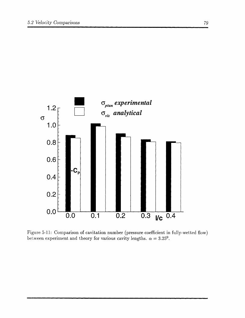
5.2 Velocity Comparisons
1.2
1.0
0.8
0.6
0.4
0.2
0.0
M
-cP
0.0
ptun experimental
(vs analytical
M
0.1
M_
0.2 0.3 Vc 0.4
Figure 5-11: Comparison of cavitation number (pressure coefficient in fully-wetted flow)between experiment and theory for various cavity lengths. a = 3.250.
I_ _
- , L I I | n m
II
5.2 Velocity Comparisons
layer profile comparisons. In other words, the experimental data is shifted from the ex-
perimental coordinate system (shown in Figure 2-1) to the numerical coordinate system,
in which case the foil surface is at z = 0.
One way of finding the foil surface is to assume the viscous sublayer is approximately
linear. In this case, the experimental profile can be extrapolated using a least squares fit
to data points measured in the sublayer. However, this assumes that a sufficient amount
of points are measured in the viscous sub-layer. Since only one or two measurements
are typically obtained in the sublayer, the extrapolated location of the foil surface has
a relatively large margin of error. Instead of using this method, the lowest data point
measured is just assumed to be the foil surface (which works very well if the data is finely
spaced).
Chapter 6
Conclusions
A systematic comparison between experiment and theory has been performed for a
partially-cavitating hydrofoil. Velocity measurements near the cavity surface are com-
pared with the numerical prediction. Also, velocities are compared in the boundary layer
region and on a rectangular contour surrounding the hydrofoil. The results are in very
good agreement with those from the analysis method in the case of fully-wetted flow, but
begin to deteriorate with increasing cavity extent.
A coupled, nonlinear, inviscid cavity analysis method and a boundary layer solver
is shown to accurately predict the velocities anywhere in the flow-field in fully-wetted
flow. In this analysis method, tunnel walls are accurately modeled with an adequate
number of image singularities, representing the foil, cavity, and displacement thickness.
In cavitating conditions, the analysis method correlates well with the experiment in the
regions of inviscid flow; however, in the boundary layer region, the analysis method does
not accurately model the displacement and momentum loss of the cavity (as evidenced in
velocity profiles aft of the cavity). Lift and drag coefficients, computed from momentum
integrations, are shown to be in good agreement with those predicted from the analysis
method.
6.1 Application to Propulsor Blades
6.1 Application to Propulsor Blades
Nothing yet has been mentioned about the applicability of the present method to propul-
sor blades. The philosophy underlying the motivation to model viscous flow around
cavitating propulsors is to be extremely systematic in reaching the final goal, ensuring
that each step in the process is accurately modeled. This means starting with simple
geometries and working to more complex ones.
The present method can be extended to three-dimensional geometries by employing a
technique called the "equivalent" o along two-dimensional strips of a three-dimensional
geometry (Kinnas et al., 1994). In the case of cavitating flow, since the lift is fixed to
the designer's desire, the procedure would include finding the correct cavity length as an
input to PCPAN/SCPAN; the correct cavity length would be that which gave the correct
lift under viscous flow as in inviscid flow. Thus, the "equivalent" oa"i in viscous flow is
aio" in inviscid flow that produces the same lift coefficient. This method can be applied
to propeller blades by calculating a new "equivalent" o at each radial strip along the
blade.
Figure 4-5 can be used, for super-cavitating foils, to find the cavity length in viscous
flow which produces the same lift as an "equivalent" cavity length in inviscid flow. Similar
figures are shown in Kinnas (1994) which can be used to find the "equivalent" cavity
length for partially-cavitating foils.
Fine and Kinnas (1992) solved for the cavity solution over finite-span three-dimensional
hydrofoils using a fully nonlinear, three-dimensional cavity analysis method. In their
routine, the cavity analysis method would iteratively calculate the cavity planform at all
locations along the span. Hufford, on the other hand, (1990) solved for the fully-wetted
flow around propulsor blades by applying the two-dimensional boundary layer equations
in a strip-wise sense. Hence, one possible way to address the problem of viscous cavitat-
ing flow over three-dimensional geometries would be to apply Hufford's method on the
"compound" blade (the surface confined by both the cavity and foil surface) produced
from the method of Kinnas and Fine (1992).
6.2 Recommendations
6.2 Recommendations
This thesis attempts to further develop an analysis method for solving the viscous flow
around cavitating propulsors. This has been accomplished by using experimentation to
further study cavitation, using experimental results to validate the numerical method,
and modifying the code to give results that parallel those obtained in experiments.
Villeneuve (1993) used a strongly-coupled viscous/cavity approach, which simultane-
ously solved for the sources due to both cavity height and effects of the boundary layer.
In his method, the blowing sources were placed on the foil surface underneath the cavity.
It was noticed that Villeneuve's method became problematic when the cavity height was
large with respect to the displacement thickness.
This work rectified the problematic behavior of Villeneuve's method by using a lightly
coupled viscous/cavity approach in which case the nonlinear cavity is first determined
in inviscid flow. The blowing sources representing the boundary layer are then applied
to the cavity surface. Results presented herein have shown that this method works very
well.
However, the present method still does not correctly solve the problem. And this
can be evidenced by the fact that the dynamic boundary condition is not satisfied on
the entire extent of the cavity (see Figure 3-7). While the pressure typically does not
vary much from the cavitation number, there are some cases where the viscous cavitation
number is not well defined at all.
A strongly coupled viscous/cavity solver that places the blowing sources on the up-
dated cavity height would provide the most accurate solution to the problem of viscous
cavitating flow around hydrofoils. This could be accomplished using PCPAN/SCPAN
and CAV2D-BL in an iterative manner. Thus,
* PCPAN/SCPAN would generate the cavity solution
* CAV2D-BL would calculate the viscous flow on the present iteration's "compound"
foil
* the displacement thickness would be added to the present iteration's "compound"
6.3 Preliminary "Momentum Jump" Model
foil
* PCPAN/SCPAN would be run again, now solving for the incremental cavity height
that would make the foil satisfy both the kinematic and dynamic boundary condi-
tion
* This would update until the incremental cavity height becomes smaller than a
specified criterion
Although more accurate, this method has the trade-off of being less computationally
efficient. Kinnas et al (1994) performed two iterations of this method and found the
results not to differ much from the present method.
6.3 Preliminary "Momentum Jump" Model
Accurately modeling the energy losses caused by the cavity should be of primary focus in
the continued development of CAV2D-BL. Although, the experimental forces correlate
well with theory, the flow-field cannot accurately be modeled without the implementation
of a "momentum jump" model - which would model the momentum deficit produced by
the cavity via adding the correct amount of momentum and displacement thickness at
the trailing edge of the cavity. Figure 6-1 illustrates the concept adding a jump at
the trailing edge the cavity. To date, the current method includes only a preliminary
momentum jump. Figure 6-2 shows results from the current method of the momentum
thickness along the suction side the foil and wake surface. In this figure, AOCTE is the
value that the user specifies, which, when added just aft of the cavity, would capture the
total drag in the wake, 20T. The bottom graph in Figure 6-2 shows how the analytical
velocity profile changes, with increasing 0, to favor the experimental profile.
The current preliminary results do not accurately model the additional increase in
displacement thickness as observed by Kato (1987). Thus, the completion of the current
work lies in determining a method for calculating both b6 TE and AOCTE, which, when
applied, would produce velocity profiles similar to those observed in experiments.
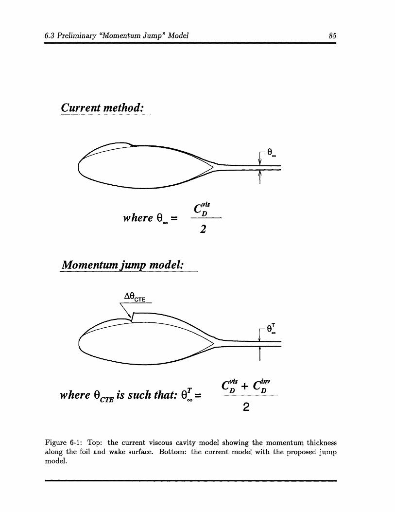
6.3 Preliminary "Momentum Jump" Model
Current method:
where O =002
Momentum jump model:
AOCTE
where O is such that: OT = + DCTE 0
Figure 6-1: Top: the current viscous cavity model showing the momentum thicknessalong the foil and wake surface. Bottom: the current model with the proposed jumpmodel.
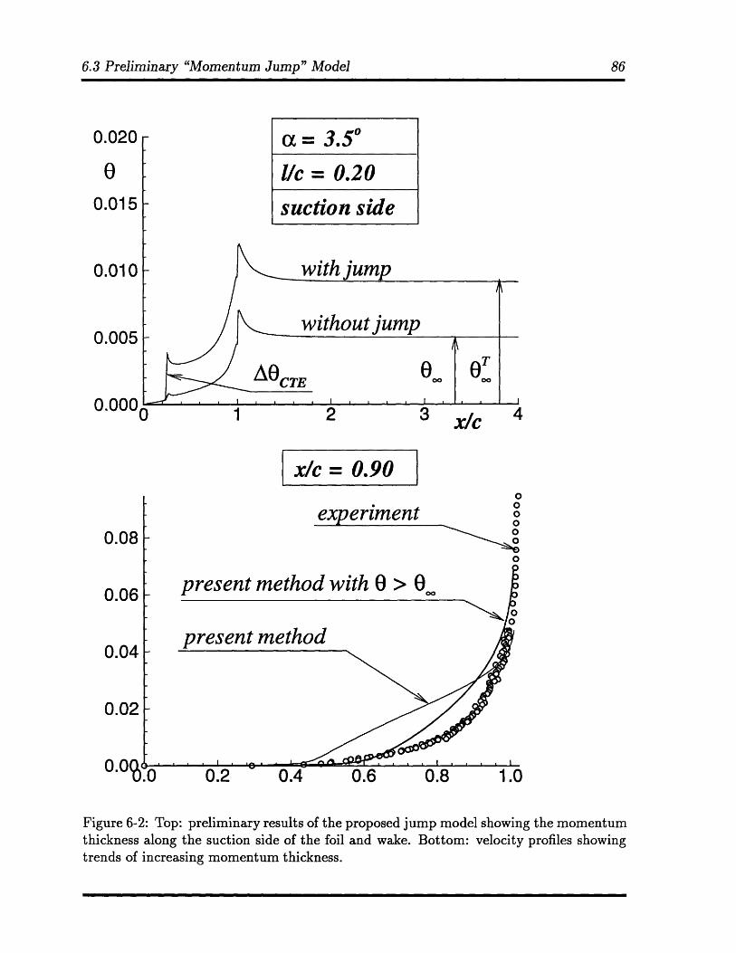
6.3 Preliminary "Momentum Jump" Model
0
0.015
0.010
0.005
'. N.I N W
1 2 3 x/c 4
x/c = 0.90
0
Figure 6-2: Top: preliminary results of the proposed jump model showing the momentumthickness along the suction side of the foil and wake. Bottom: velocity profiles showingtrends of increasing momentum thickness.
I~f% f~
I/c = 0.20
suction side
. -0
,.v 0
Bibliography
Baker, E., 1972. Analytical Prediction of Wall Effect on Fully Cavitating Lifting Foils,
Using Nonlinear Theory. Technical Report No. 3688, NSRDC.
Drela, M., 1989. XFOIL: An Analysis and Design System for Low Reynolds Number
Airfoils. In Lecture Notes in Engineering (Volume 54, Low Reynolds Number Aerody-
namics), New York. Springer-Verlag.
Fine, N., 1988. Computational and Experimental Investigations of the Flow Around
Cavitating Hydrofoils. Technical Report No. 88-6, MIT, Department of Ocean Engi-
neering.
Fine, N. and Kinnas, S., 1993. A Boundary Element Method for the Analysis of the Flow
Around 3-D Cavitating Hydrofoils. Journal of Ship Research, 37:213-224.
Franc, J. and Michel, J., 1985. Attached cavitation and the boundary layer: Experimental
investigation and numerical treatment. Journal of Fluid Mechanics, vol. 154:pp 63-90.
Geurst, J., 1959. Linearized Theory for Partially Cavitated Hydrofoils. International
Shipbuilding Progress, 6-60.
Hufford, G., 1990. Viscous Flow Around Marine Propellers Using Boundary Layer Strip
Theory. Master's thesis, Massachusetts Institute of Technology.
Kato, H., Yamaguchi, and Kubota, A., 1987. Laser Doppler Velocimeter Measurements
in Cavitation Tunnel. In Volume 2, Proceedings of the 18th International Towing Tank
Conference, pages 433-437, Kobe, SNAJ.
BIBLIOGRAPHY
Kerwin, J., 1992. The MIT Marine Hydrodynamics Water Tunnel - A 53rd Anniversary
Celebration. Presented at the New England Section SNAME Meeting, MIT.
Kinnas, S., 1991. Hydrofoil Lift and Drag from Momentum Integrations. Technical
Report No. 91-4, Department of Ocean Engineering, MIT.
Kinnas, S. and Fine, N., 1990. Non-Linear Analysis of the Flow Around Partially or
Super-Cavitating Hydrofoils by a Potential Based Panel Method. In Boundary Integral
Methods-Theory and Applications, Proceedings of the IABEM-90 Symposium, Rome,
Italy, October 15-19, 1990, pages 289-300, Heidelberg. Springer-Verlag.
Kinnas, S. and Fine, N., 1992. A nonlinear boundary element method for the analysis of
unsteady propeller sheet cavitation. In Proceedings of the Nineteenth Symposium on
Naval Hydrodynamics, Seoul, Korea.
Kinnas, S. and Fine, N., 1993. A Numerical Nonlinear Analysis of the Flow Around Two-
and Three-dimensional Partially Cavitating Hydrofoils. Journal of Fluid Mechanics,
254:151-181.
Kinnas, S. and Mazel, C., 1993. Numerical vs. Experimental Cavitation Tunnel (A
Supercavitating Hydrofoil Experiment). Journal of Fluids Engineering, 115:pp. 760-
765.
Kinnas, S., Mishima, S., and Brewer, W., 1994. Non-Linear Analysis of Viscous Flow
Around Cavitating Hydrofoils. In Proceedings of the Twentieth Symposium on Naval
Hydrodynamics, Santa Barbara, California. Office of Naval Research.
Lurie, E. H., 1993. Unsteady Response of a Two-dimensional Hydrofoil Subject to High
Reduced Frequency Gust Loading. Master's thesis, Massachusetts Institute of Tech-
nology.
Lurie, E. H., 1995. A Preliminary Note on Error Analysis of the Flapping Foil Experiment.
Technical Report No. 95-3, Department of Ocean Engineering, MIT.
BIBLIOGRAPHY
Maixner, M. R., 1977. An Experimental Investigation of Wall Effects on Supercavitat-
ing Hydrofoils of Finite Span. Technical Report No. 83481-3, Department of Ocean
Engineering, MIT.
Meijer, M., 1959. Some Experiments on Partially Cavitating Hydrofoils. International
Shipbuilding Progress, 6(60).
Press, W. H., Teukolsky, S. A., Vetterling, W. T., and Flannery, B. P., 1992. Numerical
Recipes in Fortran. Cambride University Press, New York.
Schlichting, H., 1979. Boundary-Layer Theory. McGraw-Hill, Inc.
Swafford, T., 1983. Analytical Approximation of Two-dimensional Separated Turbulent
Boundary-layer Velocity Profiles. AIAA paper, 21-6.
Uhlman, S. S. and Jinag, C.-W., 1977. Experiments on a Partially Cavitating Plano-
Convex Hydrofoil with Comparison to Theory. Technical Report No. 83481-2, MIT,
Department of Ocean Engineering.
Villeneuve, R., 1993. Effects of Viscosity on Hydrofoil Cavitation. Master's thesis,
Department of Ocean Engineering, MIT.
Wade, R., 1967. Linearized Theory of a Partially Cavitating Plano-Convex Hydrofoil
Including the Effects of Camber and Thickness. Journal of Ship Research, 11-1.
Wade, R. B. and Acosta, A. J., 1966. Experimental Observations on the Flow Past a
Plano-Convex Hydrofoil. Journal of Basic Engineering, pages 273-283.
Whitfield, D., 1978. Analytical Description of the Two-dimensional Turbulent Boundary-
layer Velocity Profile. AIAA paper, 78-1158.
Wu, T., Whitney, A., and Lin, J., 1970. Final Report: Wall Effects in Cavity Flows.
Technical Report No. E-97A-18, California Institute of Technology.
Appendix A
Calculating Displacement Thickness
In order to calculate the displacement thickness from the measured velocity profile, the
data must be integrated either numerically or analytically. However, due to the physical
limitations' of the LDV we could not measure the entire boundary layer profile (see
Figure A-1), so numerical integration cannot accurately estimate the area under the
missing region. Hence we must extrapolate the profile in that region.
In order to extrapolate the profile in this region, the following method was used (Press
et al., 1992):
* a power law curve of the following general form is fit to the existing points:
u(z) = (Az + B)(z - zo) (A.1)
* least squares can then be used to minimize the sum of the squares
N
G(a) = -[(uexp)i - u(zi; A, B, zo, n)]2 (A.2)i=1
where a = [A B z, n]
* by requiring
1We were not able to rotate the beams to measure the tangential component of the velocity near thefoil surface. At stations near the trailing edge, where the foil surface was at a larger angle, one beamwould become occluded as we tried to measure horizontal velocities
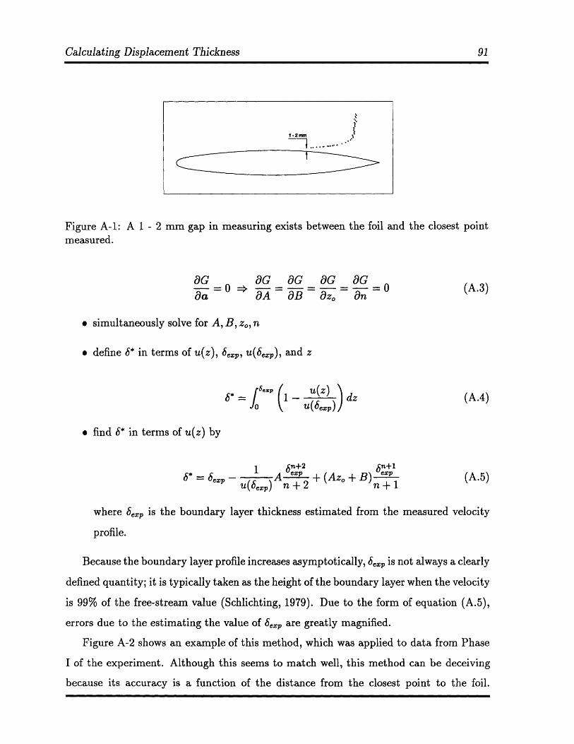
Calculating Displacement Thickness
Figure A-1: A 1 - 2 mm gap in measuring exists between the foil and the closest pointmeasured.
aG dG aG G G-O - 0 O (A.3)
9a OA &B 9z, an
* simultaneously solve for A, B, zo, n
* define 6* in terms of u(z), 6e,,, u(epp), and z
6* = 16ez ( , U (bxp) ) dz (A.4)
* find 6* in terms of u(z) by
1 6"+2 6n+1= bep A e + (Azo + B) e'x (A.5)
Su(bep) n + 2 n + 1
where bs,• is the boundary layer thickness estimated from the measured velocity
profile.
Because the boundary layer profile increases asymptotically, exp is not always a clearly
defined quantity; it is typically taken as the height of the boundary layer when the velocity
is 99% of the free-stream value (Schlichting, 1979). Due to the form of equation (A.5),
errors due to the estimating the value of 6,., are greatly magnified.
Figure A-2 shows an example of this method, which was applied to data from Phase
I of the experiment. Although this seems to match well, this method can be deceiving
because its accuracy is a function of the distance from the closest point to the foil.
1 o2mm
! ·. ... o ..

Calculating Displacement Thickness 92
Therefore, the method should only be used in cases where the LDV measures extremely
close to the foil.
__ _
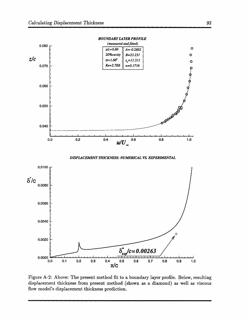
BOUNDARY LAYER PROFILE(measured and fitted)
x/c=0.89 A=-0.2862 020%cavity B=23.231 0
a=1.66 z.o=11.511 0
Re=2.7E6 n=O. 1716
I , I I .I I II
0.4 0.6•U/
DISPLACEMENT THICKNESS: NUMERICAL VS. EXPERIMENTAL
0.1 0.2 0.3 0.4 0.5 0.6 0.7 0.8 0.9 1.0x/c
Figure A-2: Above: The present method fit to a boundary layer profile. Below, resultingdisplacement thickness from present method (shown as a diamond) as well as viscousflow model's displacement thickness prediction.
Calculating Displacement Thickness
0.080
z/C0.070
0.060
0.050
0.040
0.0100
6*/c0.0080
0.0060
0.0040
0.0020
0.00000.0
E
E
Appendix B
Boundary Layer Construction
The boundary layer solver gives such integral quantities as the displacement thickness,
6*, the momentum thickness, 0, and the shape factor, H. However, it does not give
any insight of the shape of the boundary layer. Swafford (1983) presents a method of
constructing two-dimensional turbulent boundary layers from H and Ree.
The method is based on Whitfield's method (Whitfield, 1978) which composes the
boundary layer of an inner and outer solution. The inner solution is able to treat both
attached and separated flow and is given by the first term in equation (B.1). The outer
solution must vanish near the wall and reach unity as it approaches infinity. The following
equation meets both requirements:
u+ - tan-1(0.09y+)0.09
+(u - ) tanhl/2[a( )'] (B.1)
where u+ is the mean stream-wise velocity normalized on the wall-friction velocity,
TVw, u+ is the inner-law edge velocity, y+ is the non-dimensional vertical distance,
and s is a sign indicator, equal to one for attached flow and minus one for separated flow.
These equations are given by:
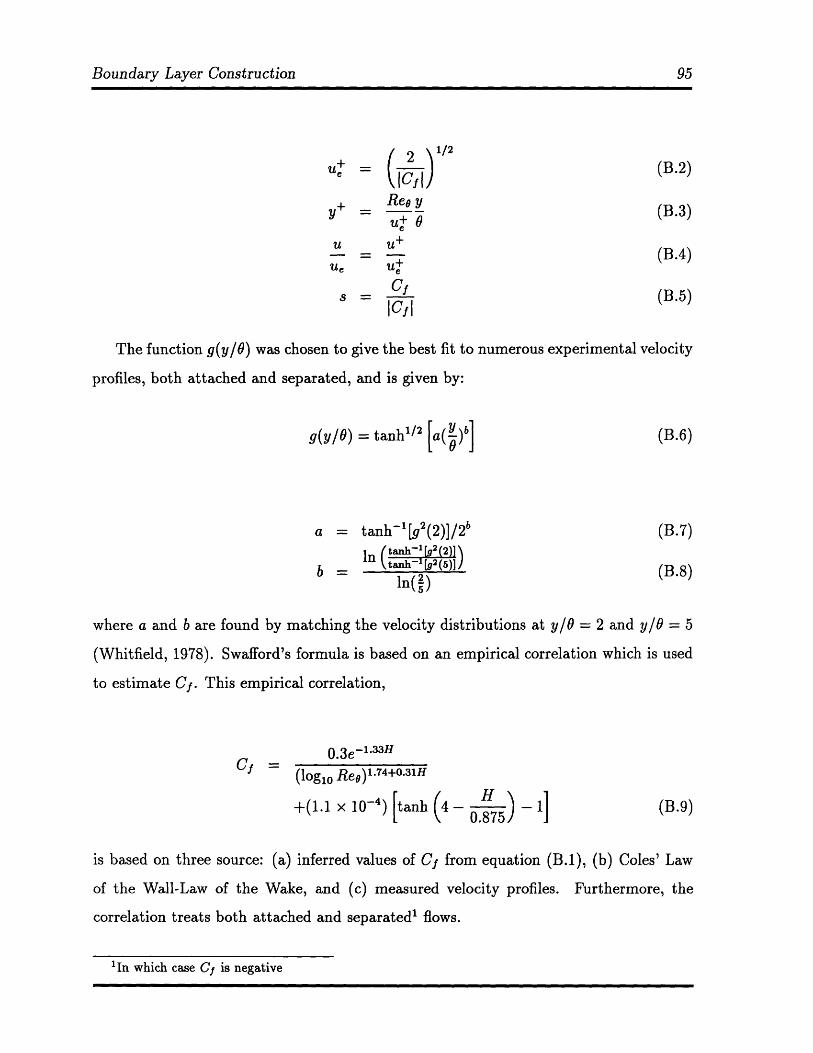
Boundary Layer Construction
U+ ( 12j (B.2)
S Rey (B.3)u+ 0
u u +
-- (B.4)Ue u
s Cf (B.5)ICl I
The function g(y/O) was chosen to give the best fit to numerous experimental velocity
profiles, both attached and separated, and is given by:
g(y/O) = tanh1 2 [a(y)b] (B.6)
a = tanh-l[g 2 (2)]/2b (B.7)In (tanh - [g2(2)]
b = tanh [g(5)] (B.8)lIn(2)
where a and b are found by matching the velocity distributions at y/O = 2 and y/O = 5
(Whitfield, 1978). Swafford's formula is based on an empirical correlation which is used
to estimate Cf. This empirical correlation,
0.3e-1.33 H
Cf = (log, 0 Reo) 1.74 +0 .31 H
+(1.1 x 10-) [tanh (4 - (B9)0.875)
is based on three source: (a) inferred values of Cf from equation (B.1), (b) Coles' Law
of the Wall-Law of the Wake, and (c) measured velocity profiles. Furthermore, the
correlation treats both attached and separated' flows.
'In which case Cj is negative

Appendix C
Experimental Data: Phase I
Figures C-1 - C-5 show all the velocity measurements taken in the boundary layer region
during Phase I of the experiment. The data has been normalized with a free-stream
velocity of 25 ft/s and a chord length of 12 in.
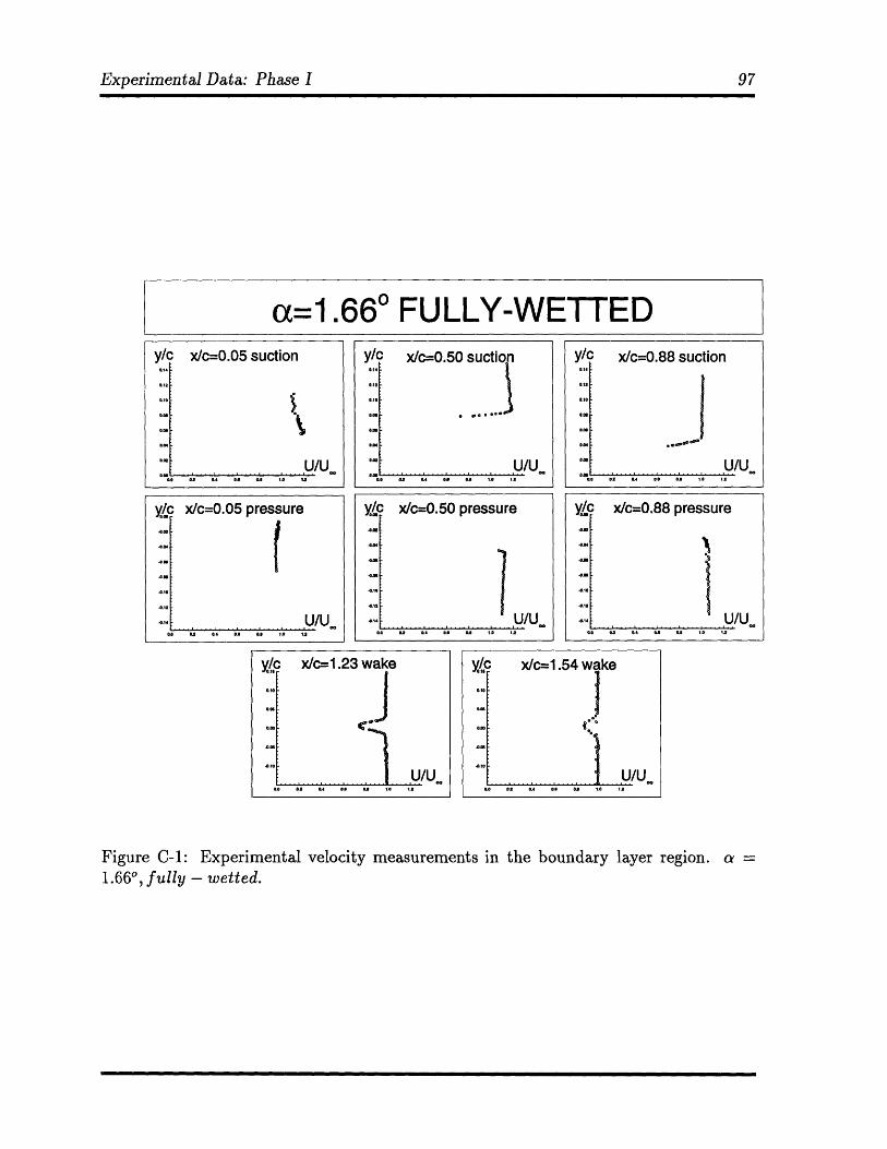
Experimental Data: Phase I
a=1.660 FULLY-WETTEDY/c x/c=0.05 suction
RIO
am
a."
.. ,
0.02 U/Uas 02 A0 OR 0.8 Is Is
y/C x/c=0.50 suction0. 14
on ' ' o, u Il1
y/c x/c=0.88 suction
ac x/c=0.50 pressure
.0.1 0 u/uS............... U /U
0.o a 0.o oR aso 1. t
YLI
y/,c x/c=1.54 wake0.1j
oa/
-.m
U/UO.0 o s .4 as *A 1. 1.2
Figure C-1: Experimental velocity measurements in the boundary layer region. a =1.660, fully - wetted.
yL/: x/c=0u.u pressure
.u.. U/U
U/U0. 0. as s 0.0 Is 1.9
x/c=0.88 pressure
. U/U
0,14
0.12
SU
-0.12
-0.14
-0.12
"014
AO o 24 oas• 1.o 1.20.0 02 0.4 OR a's 1.0 I1
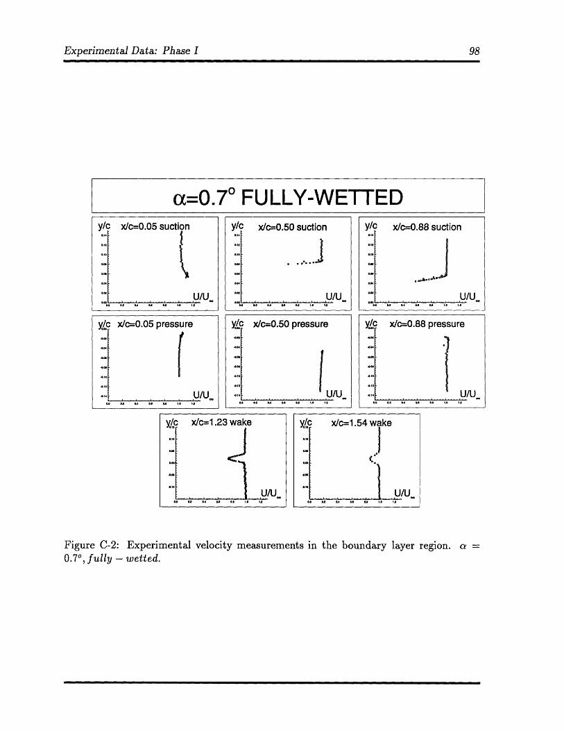
Experimental Data: Phase I 98
a=0.70 FULLY-WETTEDy/c x/c=0.05 suctionar14
a0r
D.Io
as
0.00L0
D.IN
. . . . .U/Uo o o .. .u . . io 1"
yL0
Xy/c x/c=1.23 wake
ou/ 0
U/U.tn 0e .4 to oIk o 12
y/c x/c=0.88 suction
00c x/c=0.88 pressure
.0.1 2 s. . u/u0.0 0.2 0,4 O 1.o 1.
Xy.c x/c=1.54 wake
ame
U/U0O 0.10 OA O 0 I 1.
oa s a ea a 1 l
Figure C-2: Experimental velocity measurements in the boundary layer region. a =0.70, fully - wetted.
x/c=0.50 suction
U/UI el A oA O 1o r12
J0,0l~ x/c=0.50 pressure
.u . .. U/U
t ...............0.14
U/U
0 x/c=005 ressure,.,, · V , . I''- -"-
-A02
a
It.
1.
.o o• 4 C a as .0 1. 2.
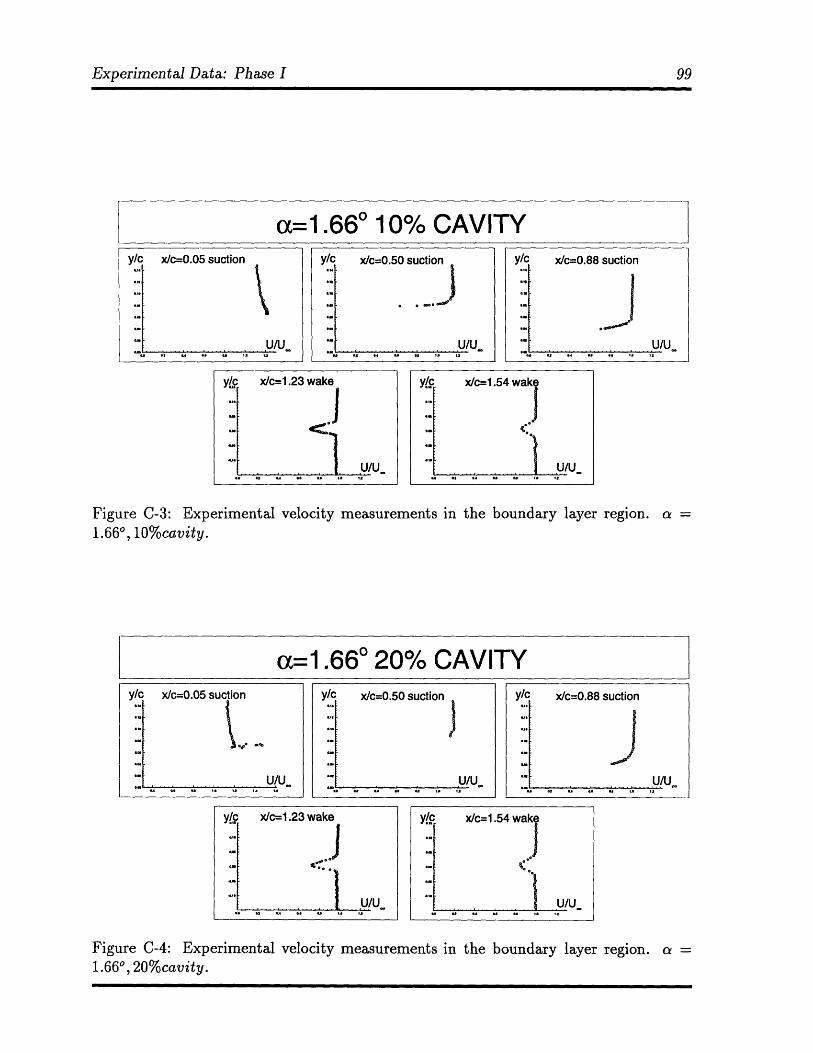
Experimental Data: Phase I
ao=1.660 10% CAVITYy/c x/c=0.05 suction
o., U 1 i
Figure C-3: Experimental velocity measurements in the boundary layer region. a =1.660, 10%cavity.
a=1.660 20% CAVITY
Y/C x/c=0.05 suction
U/U
Y/c x/c=0.50 suction
U/U
Figure C-4: Experimental velocity measurements in the boundary layer region. a =1.660, 20%cavity.
y/c x/c=0.88 suction
AnU/Uu • .no 1.
y/c x/c=1.23 wake
.jU/U-
· n o u seu u t I
y/c x/c=1.54 wake
U/U• . a s a Is
Y/C x/c=0.88 suction
U/Uon 'A 1
y/9 x/c=1.23 wake
/* 1U/U
yc x/c=1. 5 4 wak
U/U.2 u u uu 1.
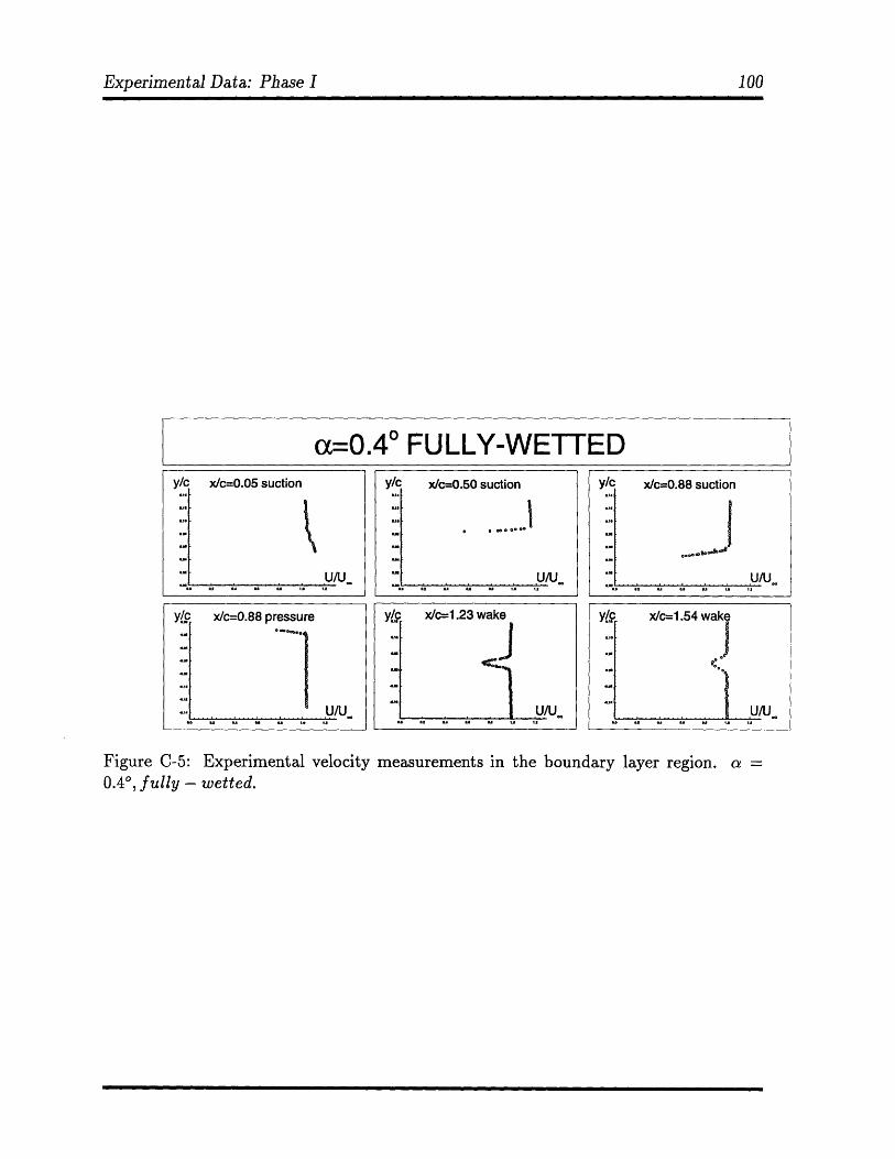
Experimental Data: Phase I 100
a=0.40 FULLY-WETTEDy/c x/c=0.05 suction
e U/Uon L i
Figure C-5: Experimental velocity measurements in the boundary layer region. a =0.40, fully - wetted.
y/c x/c=0.50 suction
0, c oo uO /
U/Uee a as s a m
y/c x/c=0.88 suction
u/ues e es a a on t .=
x/c=0.88 pressure
... 1U/Uu • u u uI IJ I,
yc x/c=1.23 wake
U/U-
y(c x/c=1.54 wake
.A.1U/U-
Experimental Data: Phase I 100
Appendix D
Experimental Versus Numerical
Results: Phase I
This appendix includes results from Phase I of the partially-cavitating hydrofoil experi-
ment. In Phase I of the experiment, the following two problems constituted a high margin
of error when compared to theory:
1. Only the horizontal beam was used in measuring the velocities in the boundary
layer region. Thus, the laser could not measure velocities within 1 - 2 mm of the
foil surface. Also, velocities measured are not those parallel to the foil.
2. The pressure side of the foil was not forced to turbulate. Therefore, the compar-
isons given in Phase I are shown as a function of laminar to turbulent transition
location. The boundary layer solver uses an e' "envelope" method to find the tran-
sition location. For this experiment, the e" method predicted a transition location
of approximately eighty percent of the chord length, which is not very likely for a
Reynold's number of three million. Figure D-3 shows several boundary layers pre-
dicted by CAV2D-BL for various transition locations. From Figure D-3, one can
infer the transition location which will produce the correct velocity profile down-
stream. Assuming that the boundary layer solver can accurately predict velocity
profiles in fully-wetted flow, which is justified in Figure D-6, then Figure D-3 shows
that the transition location tends towards x/c = 0.1 rather than x/c = 0.8. This
101
Experimental Versus Numerical Results: Phase I
same behavior is evident in the wake as shown Figure D-4. Since the displacement
thickness grows downstream, Figure D-4 is a much more sensitive measure of the
transition location than D-6.
Cavity shapes and corresponding pressure distributions are shown in Figures D-1 - D-
2. Figure D-2 is particularly interesting, a case where two cavities formed on the hydrofoil:
leading edge cavitation and bubble/midchord cavitation. Two cavities were generated by
first producing the leading edge cavity using PCPAN, then using the "compound" foil as
an input to PCPAN, to generate the midchord cavity. The pressure distribution shown
in Figure D-2 shows two cavitation numbers, which means the leading edge cavity does
not satisfy the dynamic boundary condition.
Figure D-5 - D-6 compare velocity profiles between experiment and theory. Each
profile is taken on the suction side of the foil. Figure D-5 shows essential differences in
the shape of the boundary layer due to the increased momentum deficit owing to the
cavity (see Section 5.2.3).
Finally, lift and drag coefficients are plotted against transition location in Figures D-7
- D-9. These results are very displeasing, but with all the many corrections made since
Phase I, the current lift and drag are shown to agree very well with theory as shown in
Figure 5-1.
No conclusion should be contrived, as to the accuracy of the numerical method, from
the comparisons shown in this Appendix. The intention of this data is to present a
collectively exhaustive set of data from which people may learn what works and what
does not.
102
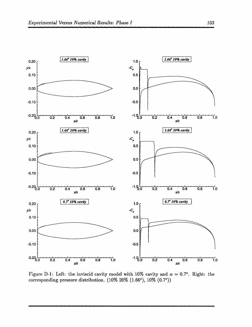
Experimental Versus Numerical Results: Phase I
11.66" 10% cavity
0 0.2 0.4 0.6 0.8 1.0x/c
-1.66" 20% cavity I
-C
) 0.2 0.4 0.6 0.8 1.0.x/c
4 ^ S1.66" 10% cavity
0.7" 10% cavity
0.2 0.4 0.6 0.8 1.0x/c
in l7 f mL .enuil, I
Figure D-1: Left: the inviscid cavity model with 10% cavity and a = 0.70. Right: thecorresponding pressure distribution. (10% 20% (1.660), 10% (0.70))
103
0.20
y/c
0.10
0.00
0.20
y/c
0.10
0.00
10
U."U
y/c
0.10
0.00
10
-4
I . . . . I . . . . I . . . . I . . . . I
-
n n~
-4
E
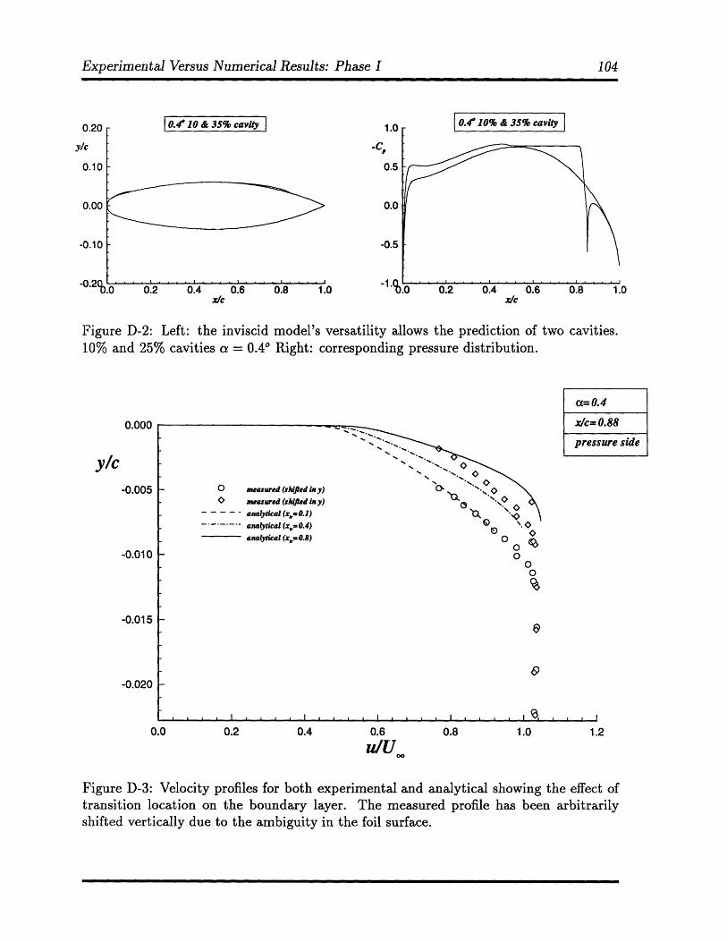
Experimental Versus Numerical Results: Phase I 104
0.4 10 & 35% cavity
0.2 0.4 0.6 0.8 1.0x/c
InA rnAO l & CaL 2 ...W.. I
Figure D-2: Left: the inviscid model's versatility allows the prediction of two cavities.10% and 25% cavities a = 0.40 Right: corresponding pressure distribution.
0.000
y/c-0.005
-0.010
-0.015
-0.020
0.0
Figure D-3: Velocity profiles for both experimental and analytical showing the effect oftransition location on the boundary layer. The measured profile has been arbitrarilyshifted vertically due to the ambiguity in the foil surface.
0.20
y/c0.10
0.00
10
O measured (shifted in y)0 measured (shifed in y)
----. analytical (x.=0.1)
- .--..-.- analytical (x,= 0.4)
analytical (x,= 0.8)
0.2 0.4 0.6 0.8 1.0
u/U
E
Experimental Versus Numerical Results: Phase I 104
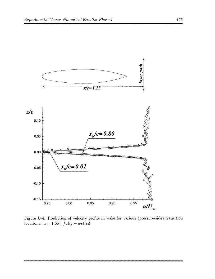
Exeimna VessNmrclRsls hs 0
x/c= 1.23
0.10
0.05
0.00
-0.05
-0.10
-0.150.75 0.80 0.85 0.90 0.95
u/U
Figure D-4: Prediction of velocity profile in wake for various (pressure-side) transitionlocations. a = 1.660, fully - wetted
IC------ i
Experimental Versus Numerical Results: Phase I 105
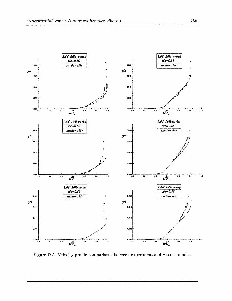
Experimental Versus Numerical Results: Phase I
1.66 fully-wettedx/c=0.50
suction side
y/c0.015
0
00
00800
0o1- I I I
0.010
0.005
0.0000.8 1.0 1.2
1.66fully-wettedx/c=0.88
suction side
o
0o
0.0 0.2 0.4 0.6W,u 0.8 1.0 1.2
1.66I 10% cavityx/c= 0.50
suction side
0
0
0.8 1.0 1.2
1.660 10% cavity
u/U
1.66* 20% cavityx/c= 0.50
suction side 0
o
0
0.8 1.0 1.2
11.66' 20% cavityl
0.0 0.2 0.4 0.6 0.8 1.0 1.2
u/U
Figure D-5: Velocity profile comparisons between experiment and viscous model.
106
0.020
0.015
0.010
0.005
nntnn
0.0 0.2 0.4 0.6uUw
0.020
y/c0.015
0.010
0.005
n n000.0 0.2 0.4 0.6
u/U.
0.020
y/c0.015
0.010
0.005
2
0.0 0.2 0.4 0.6
u/Um
. . . - -- - - , , i , , ' ' ' ' ' ' ' '
-
-
-
-
-
u.vw0.0
L
M
(
E
E
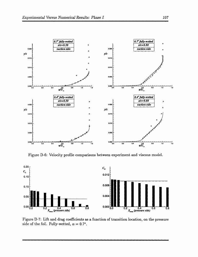
Experimental Versus Numerical Results: Phase I
0.7 fully-wettedx/c=0.50
suction side
0.......
0.020
0.005
n ,•0.8 1.0 1.2 0.0
0.7 fully-wetted
0.2 0.4 0.6
&/l m0.8 1.0 1.2
0.4 fully-wettedx/c= 0.50
suction side
0.8 1.0 1.2
0./ fully-wetted I
W/U_
Figure D-6: Velocity profile comparisons between experiment and viscous model.
0.20
C,
0.15-
CD
0.012-
0.10 0.008
0.05 0 0.004
0.00 0.0000.0 0.2 0.4 0.6 0.8 0.0 0.2 0.4 0.6 0.8
X,,. (pressure side) X. (pressure side)
Figure D-7: Lift and drag coefficients as a function of transition location, on the pressureside of the foil. Fully-wetted, a = 0.70.
107
0.020
0.015
0.0 0.2 0.4 0.6u/U
0.020
Y/c0.015
0.010
0.005
0l 0000.0 0.2 0.4 0.6
u/U2
-
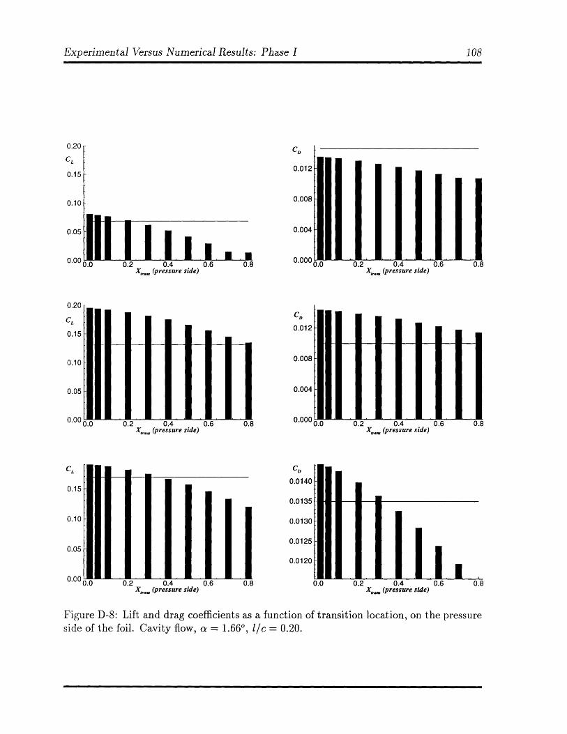
Experimental Versus Numerical Results: Phase I
K U-
CD
0.012
0.008
0.004
0 n00II lli, ..0.2 0.4 0.6
X,, (pressure side)0.0 0.2 0.4 0.6
XX, (pressure side)
C,
0.0140
0.0135
0.0130
0.0125
0.0120
X,•.. (pressure side)0.0 0.2 0.4 0.6
X,, (pressure side)
Figure D-8: Lift and drag coefficients as a function of transition location, on the pressureside of the foil. Cavity flow, a = 1.660, 1/c = 0.20.
0.20
C,
0.15
0.10
0.05
0.00 0
I
._...,_.a u__...,,_.a
-
-
-
ill,.
108
.0, L
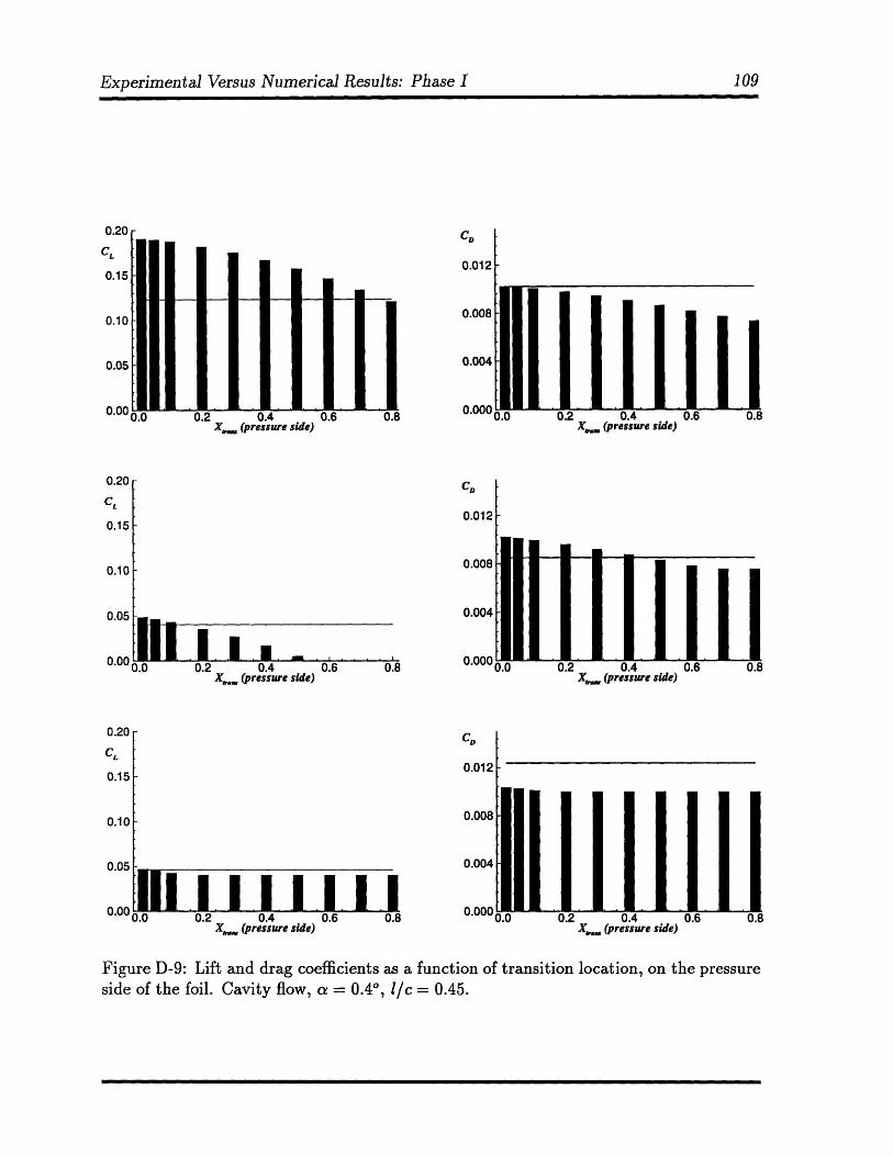
Experimental Versus Numerical Results: Phase I 109
0.20
CL
0.15
0.10
0.05
0.00
0.20
CL
0.15
0.10
0.05
0.00
111 I .0.0 0.2 0.4 0.6 0.8
X.., (pressure side)
0.0 0.2 0.4 0.6X,.. (pressure side)
0.008
0.004
0.000 0.2 0.4 0.6 0.8X. (pressure side)
CD
0.012
0.008
0.004
0.000 0.0 0.2 0.4 0.6 0.8X~. (pressure side)
X,. (pressure side)
Figure D-9: Lift and drag coefficients as a function of transition location, on the pressureside of the foil. Cavity flow, a = 0.40, 1/c = 0.45.
-- -- --
Experimental Versus Numerical Results: Phase I 109