Embed Size (px)
Citation preview
ME5311 Computational Methods of Viscous Fluid Dynamics
Instructor: Prof. Zhuyin Ren
Department of Mechanical EngineeringUniversity of Connecticut
Spring 2013

Conservation Laws
Conservation laws can be derived either using a
Control Mass approach (CM) o Considers a fixed mass (useful for solids) and its extensive properties (mass, momentum
and energy)
Control Volume approach (CV) o CV is a certain spatial region of the flow, possibly moving with fluid parcels/system
o Its surfaces are control surfaces (CS)
Each approach leads to a class of numerical methods
For an extensive property, the conservation law “relates the rate of change of the property in the CM to externally determined effects on this property”
To derive local differential equations, assumption of continuum is made –Knudsen number (mean free path over length-scale, λ/L < 0.01)
o => Sufficiently “well behaved” continuous functions
o Non-continuum flows: space shuttle in reentry, low-pressure processing
Note CFD is also used for Newton’s law applied to each constituent molecules (simple, but computational cost often growths as N2 or more)

Macroscopic Properties

Observed Influence of the Reynolds Number
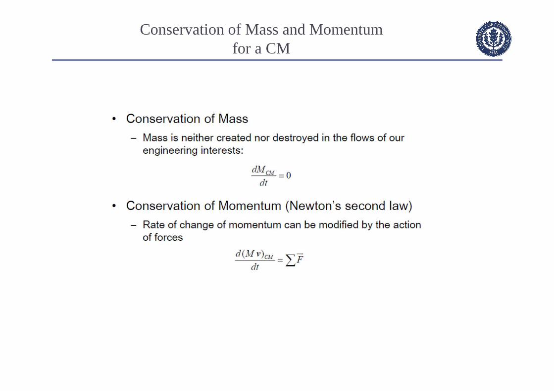
Conservation of Mass and Momentumfor a CM
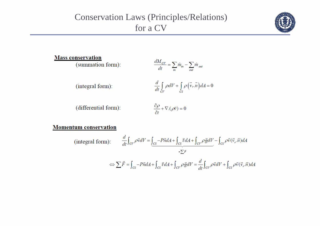
Conservation Laws (Principles/Relations)for a CV
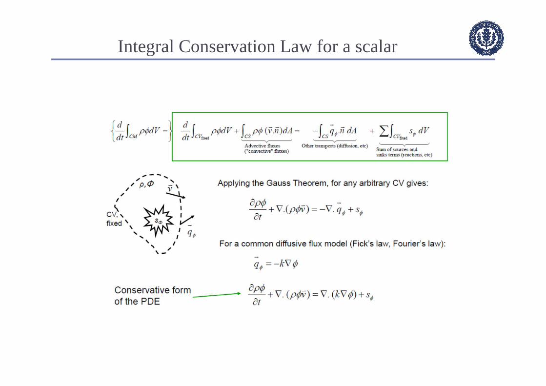
Integral Conservation Law for a scalar

Strong-Conservative formof the Navier-Stokes Equations
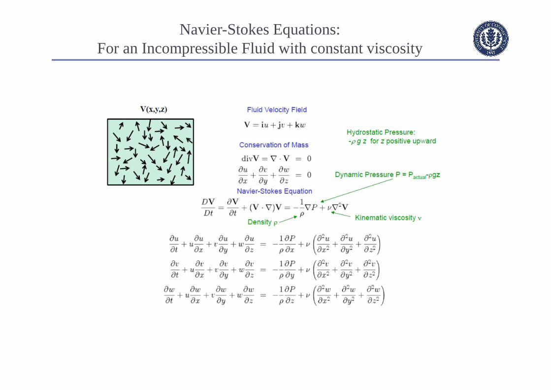
Navier-Stokes Equations:For an Incompressible Fluid with constant viscosity

Incompressible FluidPressure Equation

Inviscid Fluid MechanicsEuler’s Equation

Turbulence Modeling
Outline
Background Characteristics of Turbulent Flow
o Scales
Eliminating the small scaleso Reynolds Averaging
o Filtered Equations
Turbulence Modeling Theory RANS Turbulence Models in FLUENT
Turbulence Modeling Options in Fluent Near wall modeling, Large Eddy Simulation (LES)
Turbulent Flow Examples Comparison with Experiments and DNS
o Turbulence Models
o Near Wall Treatments

What is Turbulence?
Unsteady, irregular (aperiodic) motion in which transported quantities (mass, momentum, scalar species) fluctuate in time and space
Fluid properties exhibit random variations statistical averaging results in accountable, turbulence related transport
mechanisms
Contains a wide range of eddy sizes (scales) typical identifiable swirling patterns
large eddies ‘carry’ small eddies
http://www.youtube.com/watch?v=AeBsiEYWZUY

Turbulent boundary layer on a flat plate
Homogeneous, decaying, grid-generated turbulence
Two Examples of Turbulence

Energy Cascade
Larger, higher-energy eddies, transfer energy to smaller eddies via vortex stretching Larger eddies derive energy from mean flow
Large eddy size and velocity on order of mean flow
Smallest eddies convert kinetic energy into thermal energy via viscous dissipation Rate at which energy is dissipated is set by rate at which they receive
energy from the larger eddies at start of cascade

Vortex Stretching
Existence of eddies implies vorticity
Vorticity is concentrated along vortex lines or bundles
Vortex lines/bundles become distorted from the induced velocities of the larger eddies As end points of a vortex line randomly move apart
o vortex line increases in length but decreases in diameter
o vorticity increases because angular momentum is nearly conserved
Most of the vorticity is contained within the smallest eddies
Turbulence is a highly 3D phenomenon
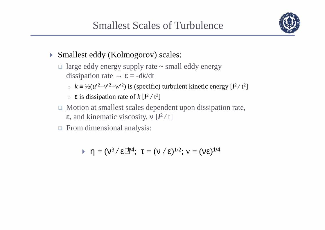
Smallest Scales of Turbulence
Smallest eddy (Kolmogorov) scales: large eddy energy supply rate ~ small eddy energy
dissipation rate → ε = -dk/dto k ≡ ½(u′2+v′2+w′2) is (specific) turbulent kinetic energy [l2 / t2]
o ε is dissipation rate of k [l2 / t3]
Motion at smallest scales dependent upon dissipation rate, ε, and kinematic viscosity, ν [l2 / t]
From dimensional analysis:
η = (ν3 / ε)1/4; τ = (ν / ε)1/2; v = (νε)1/4
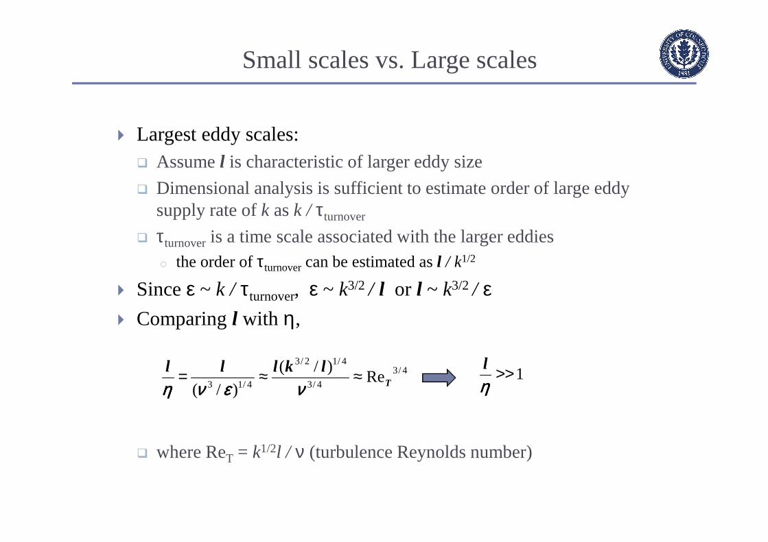
Small scales vs. Large scales
Largest eddy scales: Assume l is characteristic of larger eddy size
Dimensional analysis is sufficient to estimate order of large eddy supply rate of k as k / τturnover
τturnoveris a time scale associated with the larger eddieso the order of τturnovercan be estimated as l / k1/2
Since ε ~ k / τturnover, ε ~ k3/2 / l or l ~ k3/2 / ε Comparing l with η,
where ReT = k1/2l / ν (turbulence Reynolds number)
4/3
4/3
4/12/3
4/13Re
)/(
)/( T
lklll ≈≈=ννννεεεεννννηηηη
1>>ηηηηl

Implication of Scales
Consider a mesh fine enough to resolve smallest eddies and large enough to capture mean flow features
Example: 2D channel flow
Ncells~(4l / η)3
or
Ncells ~ (3Reτ)9/4
where
Reτ = uτH / 2ν ReH = 30,800 → Reτ = 800 → Ncells = 4x10⁷ !
H4/13 )/( ενη
ll ≈
l
η

Direct Numerical Simulation
“DNS” is the solution of the time-dependent Navier-Stokes equations without recourse to modeling
Numerical time step size required, ∆t ~ τo For 2D channel example
ReH = 30,800
Number of time steps ~ 48,000
DNS is not suitable for practical industrial CFDo DNS is feasible only for simple geometries and low turbulent
Reynolds numbers
o DNS is a useful research tool
∂∂
∂∂+
∂∂−=
∂∂+
∂∂
j
i
kik
ik
i
x
U
xx
p
x
UU
t
U µρ
ττ u
Ht ChannelD
Re
003.02 ≈∆

Removing the Small Scales
Two methods can be used to eliminate need to resolve small scales: Reynolds Averaging
o Transport equations for mean flow quantities are solved
o All scales of turbulence are modeled
o Transient solution ∆t is set by global unsteadiness
Filtering (LES)o Transport equations for ‘resolvable scales’
o Resolves larger eddies; models smaller ones
o Inherently unsteady, ∆t set by small eddies
Both methods introduce additional terms that must be modeled for closure

l η = l/ReT3/4
Prediction Methods

RANS Modeling - Velocity Decomposition
Consider a point in the given flow field:
( ) ( ) ( )txutxUtxu iii ,,,rrr ′+=
u'i
Ui ui
time
u

RANS Modeling - Ensemble Averaging
Ensemble (Phase) average:
Applicable to nonstationary flows such as periodic or quasi-periodic flows involving deterministic structures
( ) ( )( )∑=∞→
=N
n
ni
Ni txu
NtxU
1
,1
lim,rr
U
( )
∂′+∂
∂∂+
∂′+∂−=
∂′+∂′++
∂′+∂
j
ii
jik
iikk
ii
x
uU
xx
pp
x
uUuU
t
uU )()()(
)( µρ
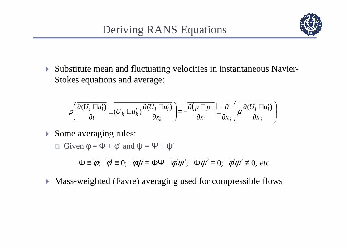
.,0;0;;0; etc≠′′=′Φ′′+ΦΨ=≡′≡Φ ψφψψφφψφφ
Deriving RANS Equations
Substitute mean and fluctuating velocities in instantaneous Navier-Stokes equations and average:
Some averaging rules: Given φ = Φ + φ′ and ψ = Ψ + ψ′
Mass-weighted (Favre) averaging used for compressible flows

RANS Equations
Reynolds Averaged Navier-Stokes equations:
New equations are identical to original except : The transported variables, U, ρ, etc., now represent the mean
flow quantities
Additional terms appear:o Rij are called the Reynolds Stresses
Effectively a stress→
o These are the terms to be modeled
( )j
ji
j
i
jik
ik
i
x
uu
x
U
xx
p
x
UU
t
U
∂−∂
+
∂∂
∂∂+
∂∂−=
∂∂+
∂∂ ρ
µρ
jiij uuR ρ−=
−
∂∂
∂∂
jij
i
j
uux
U
xρµ
(prime notation dropped)
Turbulence Modeling Approaches
Boussinesq approach isotropic
relies on dimensional analysis
Reynolds stress transport models no assumption of isotropy
contains more “physics”
most complex and computationally expensive

The Boussinesq Approach
Relates the Reynolds stresses to the mean flow by a turbulent (eddy) viscosity, µt
Relation is drawn from analogy with molecular transport of momentum
Assumptions valid at molecular level, not necessarily valid at macroscopic levelo µt is a scalar (Rij aligned with strain-rate tensor, Sij)
o Taylor series expansion valid if lmfp|d2U/dy2| << |dU/dy|
o Average time between collisions lmfp / vth << |dU/dy|-1
∂∂
+∂∂=−
∂∂−=−=
i
j
j
iijijij
k
kijjiij x
U
x
USk
x
USuuR
21
;32
32
2 tt δρδµµρ
ijxy Svut µρ 2=′′′′−=

Modeling µµµµt
Oh well, focus attention on modeling µt anyways
Basic approach made through dimensional arguments Units of νt = µt/ρ are [m2/s]
Typically one needs 2 out of the 3 scales:o velocity - length - time
Models classified in terms of number of transport equations solved, e.g., zero-equation
one-equation
two-equation
…

Zero Equation Model
Prandtl mixing lengthmodel: Relation is drawn from same analogy with molecular transport of
momentum:
The mixing length model:o assumes that vmix is proportional to lmix& strain rate:
o requires that lmix be prescribed lmix must be ‘calibrated’ for each problem
Very crude approach, but economicalo Not suitable for general purpose CFD though can be useful where a
very crude estimate of turbulence is required
∂∂
+∂∂==
i
j
j
iijijijmixt x
U
x
USSSl
2
1;22ρµ
mfpthv2
1lρµ = mixmixv
2
1lt ρµ =
ijij SSl 2v mixmix ∝
Other Zero Equation Models
Mixing length observed to behave differently in flows near solid boundaries than in free shear flows Modifications made to the Prandtl mixing length model to account for
near wall flowso Van Driest- Reduce mixing length in viscous sublayer (inner boundary layer)
with damping factor to effect reduced ‘mixing’o Clauser- Define appropriate mixing length in velocity defect (outer boundary)
layero Klebanoff- Account for intermittency dependencyo Cebeci-Smith and Baldwin-Lomax
Accounts for all of above adjustments in two layer models
Mixing length models typically fail for separating flows Large eddies persist in the mean flow and cannot be modeled from local
properties alone

One-Equation Models
Traditionally, one-equation models were based on transport equation for k (turbulent kinetic energy) to calculate velocity scale, v = k1/2
Circumvents assumed relationship between v and turbulence length scale (mixing)
Use of transport equation allows ‘history effects’ to be accounted for
Length scale still specified algebraically based on the mean flow very dependent on problem type
approach not suited to general purpose CFD

−−
∂∂
∂∂+−
∂∂=
∂∂+
∂∂
jjiijjj
iij
jj upuuu
x
k
xx
UR
x
kU
t
k'
2
1 ρµρερ
unsteady &convective
productiondissipation
molecular
diffusion
turbulent
transport
pressure
diffusion
k
i
k
i
x
u
x
u
∂∂
∂∂=νε
Turbulence Kinetic Energy Equation
Exact k equation derived from sum of products of Navier-Stokes equations with fluctuating velocities (Trace of the Reynolds Stress transport equations)
where (incompressible form)

Modeled Equation for k
The production, dissipation, turbulent transport, and pressure diffusion terms must be modeled Rij in production term is calculated from Boussinesq formula
Turbulent transport and pressure diffusion:
ε = CDk3/2/l from dimensional arguments
µt = CDρk2/ ε (recall µt ∝ ρk1/2l)
CD, σk, and l are model parameters to be specifiedo Necessity to specify l limits usefulness of this model
Advanced one equation models are ‘complete’ solves for eddy viscosity
jkjjii x
kupuuu
∂∂−=+
σµρ t'
21 Using µt/σk assumes k
can be transported by turbulence as can U

Spalart-Allmaras Model Equations
ννχ
χχνρµ
~,f ,~
3
1
3
3
v11t ≡+
=≡cv
vf
1v2222 1
1f ,~~
vv f
fd
SSχχ
κν
+−=+≡
( )22
62
6/1
6
3
6
6
3~
~,g ,
1
dSrrrcr
ggf w
w
ww
cc
κν≡−+=
+
+=
( )2
1
2
2~
1
~
~~~1~~~
−
∂∂+
∂∂+
∂∂+ =
dfc
xc
xxSc
Dt
Dww
jb
jjb
νρνρννρµσ
νρνρν
0~:conditionboundary Wall =ν
modified turbulent viscosity
distance from wall
damping functions

∂∂
−∂∂=ΩΩΩ≡
i
j
j
i
x
U
x
US
2
1; 2 ijijij
) - S min(0, C ijijprodij Ω+Ω≡S
Spalart-Allmaras Production Term
Default definition uses rotation rate tensor only:
Alternative formulation also uses strain rate tensor:
reduces turbulent viscosity for vortical flows
more correctly accounts for the effects of rotation

Spalart-Allmaras Model
Spalart-Allmaras model developed for unstructured codes in aerospace industry Increasingly popular for turbomachinery applications
“Low-Re” formulation by defaulto can be integrated through log layer and viscous sublayer to wall
o Fluent’s implementation can also use law-of-the-wall
Economical and accurate for:o wall-bounded flows
o flows with mild separation and recirculation
Weak for:o massively separated flows
o free shear flows
o simple decaying turbulence
Two-Equation Models
Two transport equations are solved, giving two independent scales for calculating µt
Virtually all use the transport equation for the turbulent kinetic energy, k
Several transport variables have been proposed, based on dimensional arguments, and used for second equation
o Kolmogorov, ω: µt ∝ ρk / ω, l ∝ k1/2 / ω, k ∝ ε / ω ω is specific dissipation rate defined in terms of large eddy scales that define supply rate of k
o Chou, ε: µt ∝ ρk2 / ε, l ∝ k3/2 / εo Rotta, l: µt ∝ ρk1/2l, ε ∝ k3/2 / l
Boussinesq relation still used for Reynolds Stresses

Standard k-ε Model Equations
ijijtjkj
SSSSx
k
xDt
Dk2;2t =−+
∂∂
+
∂∂= ρεµ
σµµρ
( )ερµεεσµµερ εε
ε2
2t1
t CSCkxxDt
D
jj−+
∂∂
+
∂∂=
k-transport equation
ε-transport equationproduction dissipation
2 , , , εεεσσ CCik
coefficients
turbulent viscosity
ερµ µ
2
k
Ct =
inverse time scale
Empirical constants determined from benchmark experiments of simple flows using air and water.

Simple flows render simpler model equations Coefficients can be isolated and compared with experiment
e.g.,o Uniform flow past grid
Standard k-ε equations reduce to just convection and dissipation terms
o Homogeneous Shear Flow
o Near-Wall (Log layer) Flow
kC
xU
x
kU
2
2d
d;
d
d εεε ε−=−=
Closure Coefficients

Buoyancyproduction
DilatationDissipation
RT
k
xgS
x
k
xDt
Dk
it
tit
jkj γρερ
ρµρεµ
σµµρ 2
Pr2t −
∂∂−−+
∂∂
+
∂∂=
Standard k-ε Model
High-Reynolds number model (i.e., must be modified for the near-wall region)
The term “standard” refers to the choice of coefficients
Sometimes additional terms are included production due to buoyancy
o unstable stratification (g·∇∇∇∇T >0) supports k production
dilatation dissipation due to compressibilityo added dissipation term, prevents overprediction of spreading rate in
compressible flows
Standard k-ε Model Pros & Cons
Strengths: robust
economical
reasonable accuracy for a wide range of flows
Weaknesses: overly diffusive for many situations
o flows involving strong streamline curvature, swirl, rotation, separating flows, low-Re flows
cannot predict round jet spreading rate
Variants of the k-ε model have been developed to address its deficiencies RNG and Realizable

RNG k-ε Model Equations
Derived using renormalization group theory scale-elimination technique applied to Navier-Stokes equations
(sensitizes equations to specific flow regimes)
o k equation is similar to standard k-ε model
o Additional strain rate term in ε equation most significant difference between standard and RNG k-ε models
o Analytical formula for turbulent Prandtl numbers
o Differential-viscosity relation for low Reynolds numbers Boussinesq model used by default
( ) ( ) whereCSCkxxDt
Dt
jjερµεεµαερ εεε
*2
21eff −+
∂∂
∂∂=
t
kS
C
CC
µµµβη
εη
βηηηρηµ
εε
+=
=
+
−
+=
eff
0
30
3
2*2
tscoefficienare,
1
1
ε-transport equation
RNG k-ε Model Pros &Cons
For large strain rates: where η > η0, ε is augmented, and therefore k and µt are reduced
Option to modify turbulent viscosity to account for swirl
Buoyancy and compressibility terms can be included
Improved performance over std. k-ε model for rapidly strained flows
flows with streamline curvature
Still suffers from the inherent limitations of an isotropic eddy-viscosity model

Standard k-ε model could not ensure: Positivity of normal stresses
Schwarz’s inequality of shear stresses
Modifications made to standard model k equation is same; new formulation for µt and ε Cµ is variable
ε equation is based on a transport equation for the mean-square vorticity fluctuation
02 ≥uα
( ) uuuu 222βαβα ≤
Realizable k-ε Model: Motivation

How can normal stresses become negative?
Standard k-ε Boussinesq viscosity relation:
Normal component:
Normal stress will be negative if:
3
2 - ij
2
δρε
ρρ µ kx
U
x
UkCuu
i
j
j
iji
∂∂
+∂∂=−
2 3
2
22
x
UkCku
∂∂−=
εµ
3.7 3
1 ≈>
∂∂
µε Cx
Uk
Realizable k-ε Model: Realizability
Realizable k-ε Model: Cµ
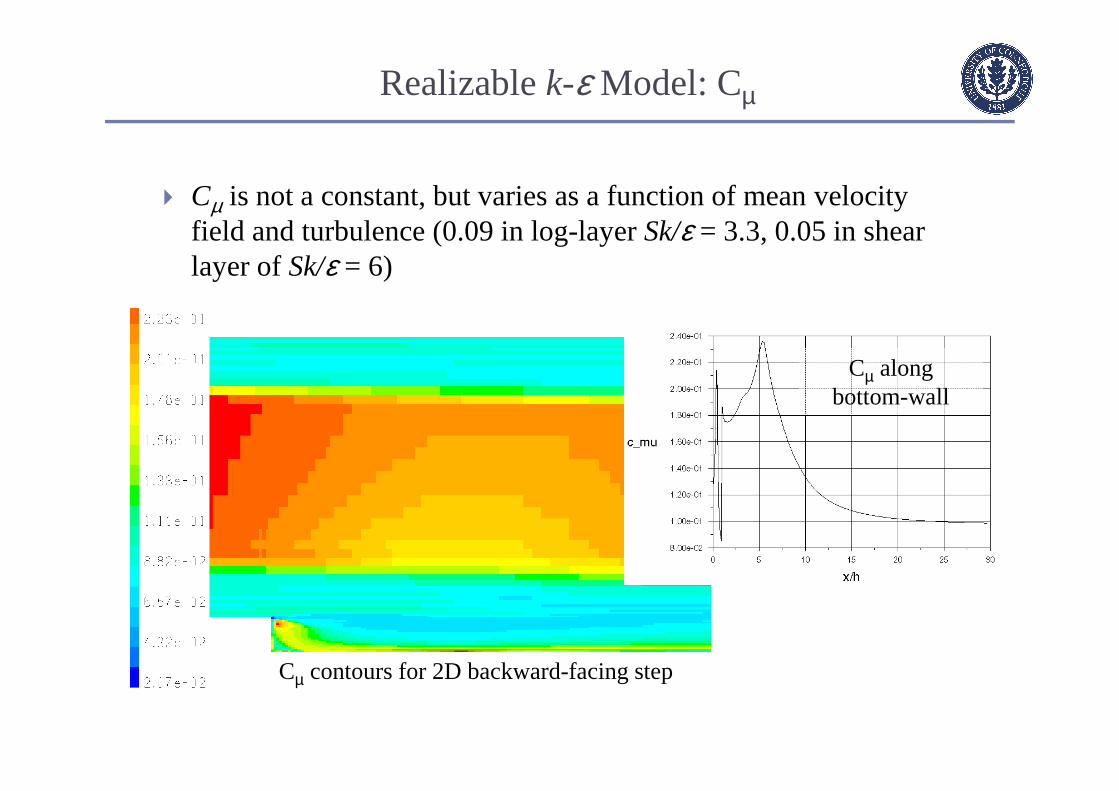
Cµ is not a constant, but varies as a function of mean velocity field and turbulence (0.09 in log-layer Sk/ε = 3.3, 0.05 in shear layer of Sk/ε = 6)
Cµ contours for 2D backward-facing step
Cµ along bottom-wall
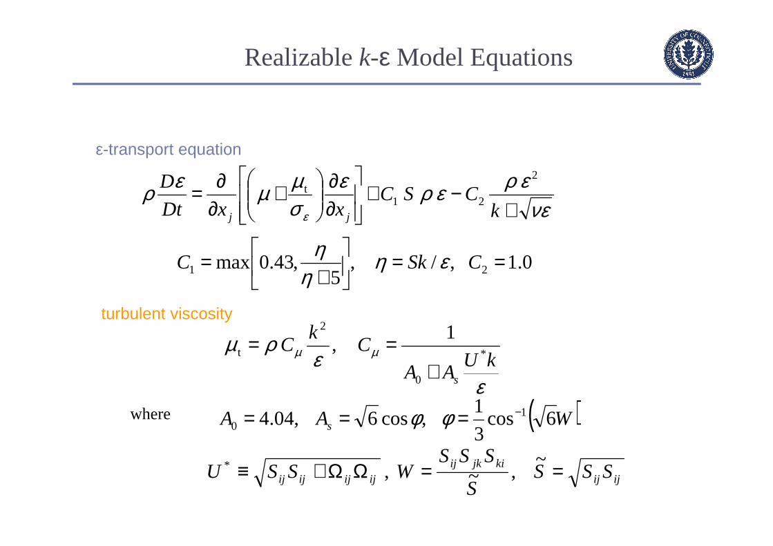
Realizable k-ε Model Equations
εε
ρµ µµ kUAA
Ck
C
s
*
0
2
t
1,
+==
where
ijijkijkij
ijijijij SSSS
SSSWSSU ==ΩΩ+≡ ~
,~ , *
( )WAA s 6cos3
1,cos6,04.4 1
0−=== φφ
0.1 ,/,5
,43.0max 21 ==
+= CSkC εη
ηη
νεερερε
σµµερ
ε +−+
∂∂
+
∂∂=
kCSC
xxDt
D
jj
2
21t
ε-transport equation
turbulent viscosity
Realizable k-ε Model Pros & Cons
Performance generally exceeds the standard k-ε model
Buoyancy and compressibilty terms can be included
Good for complex flows with large strain rates recirculation, rotation, separation, strong ∇p
Resolves the round-jet/plane jet anomaly predicts the speading rate for round and plane jets
Still suffers from the inherent limitations of an isotropic eddy-viscosity model

Standard and SSTk-ω Models
k-ω models are a popular alternative to k-ε ω ~ ε / k µt ∝ ρk / ω
Wilcox’s original model was found to be quite sensitive to inlet and far-field boundary values of ω
Can be used in near-wall region without modification
Latest version contains several refinements: reduced sensitivity to boundary conditions
modifcation for the round-jet/plane-jet anomaly
compressibility effects
low-Re (transitional) effects
Standard k-ω Model
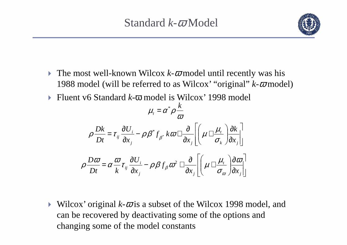
The most well-known Wilcox k-ω model until recently was his 1988 model (will be referred to as Wilcox’ “original” k-ω model)
Fluent v6 Standard k-ω model is Wilcox’ 1998 model
Wilcox’ original k-ω is a subset of the Wilcox 1998 model, and can be recovered by deactivating some of the options and changing some of the model constants
∂∂
+
∂∂+−
∂∂=
∂∂
+
∂∂+−
∂∂=
=
j
t
jj
iij
jk
t
jj
iij
t
xxf
x
U
kDt
D
x
k
xkf
x
U
Dt
Dk
k
ωσµµωβρτωαωρ
σµµωβρτρ
ωραµ
ωβ
β
2
*
*
*

Standard k-ω Turbulent Viscosity
Turbulent viscosity is computed from:
The dependency of α* upon ReT was designed to recover the correct asymptotic values in the limiting cases. In particular, note that:
ωραµ k
t*=
0.1 ,Re,6
125
9,
3,
Re1
Re where
*
*0
*0**
===
==
++
=
∞
∞
αωµρ
ββαααα
kR
R
R
Tk
ii
kT
kT
turbulent)(fully as ∞→→ TRe1*α

Standard k-ω Turbulent Kinetic Energy
Note the dependence upon ReΤ , Mt , and χk
“Dilatation” dissipation is accounted for via Mt term
The cross-diffusion parameter (χk ) is designed to improve free shear flow predictions
444 3444 2143421
321k of Diffusion
k of rate nDissipatiok of production
∂∂
+
∂∂+−
∂∂=
jk
t
jj
iij x
k
xkf
x
U
Dt
Dk
σµµωβρτρ β *
*
( )[ ]( )
( )09.0 ,5.1 ,0.2
8,Re1
Re1541
**
4
4
**
***
===
=+
+=
+=
∞
∞
βζσ
ββ
ζββ
ββ
β
k
T
Ti
ti
RR
RMF ( )
44 344 21parameter diffusion-cross
jjk
kk
k
k
tt
tttt
ttt
xx
kf
RTaMa
kM
MMMM
MMMF
∂∂
∂∂=
>++
≤=
===
>−
≤=
ωω
χχ
χχ
χ
γ
β 32
2
022
020
2
0
1,
04001
6801
01
,4
1,
2
0
*

Note the dependence upon ReΤ , Mt , and χω
Vortex-stretching parameter (χω) designed to remedy the plane/round-jet anomaly
Standard k-ω Specific Dissipation Equation
∂∂
+
∂∂+−
∂∂=
j
t
jj
iij xx
fx
U
kDt
D ωσµµωβρτωαωρ
ωβ
2
( ) ( )
∂∂
−∂∂
=Ω
∂∂
+∂∂
=
=ΩΩ
=++
=
+=
====++
=
∞
∞
∞
∞∞
i
j
j
iij
i
j
j
iij
kijkijt
i
ii
T
T
x
U
x
U
x
U
x
US
SfMF
RR
R
2
1,
2
1
5.1 ,,801
701,1
0.2,95.2,9
1,
25
13,
Re1
Re
*3*
**
00
*
ζωβ
χχχζ
ββββ
σαααααα
ωω
ωβ
ωωω
ω
Standard k-ω Model Sub-models & Options (I)
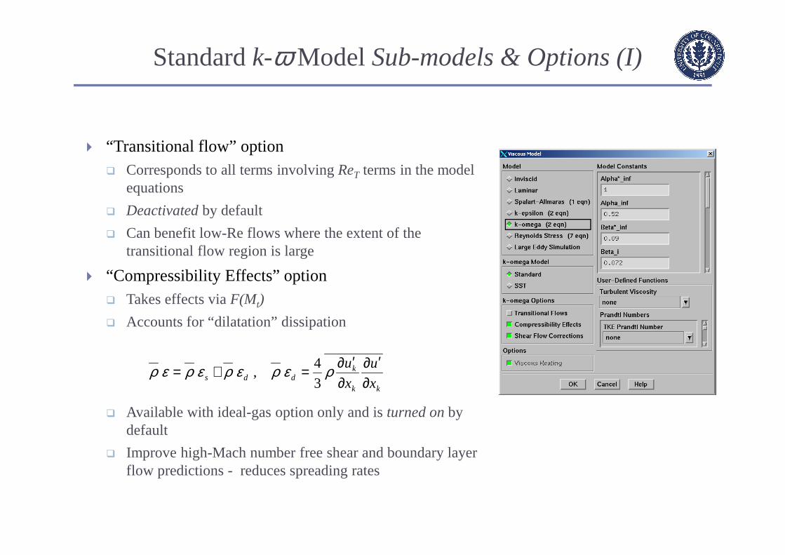
“Transitional flow” option Corresponds to all terms involving ReT terms in the model
equations
Deactivated by default
Can benefit low-Re flows where the extent of the transitional flow region is large
“Compressibility Effects” option Takes effects via F(Mt)
Accounts for “dilatation” dissipation
Available with ideal-gas option only and is turned onby default
Improve high-Mach number free shear and boundary layer flow predictions - reduces spreading rates
kk
kdds x
u
x
u
∂′∂
∂′∂=+= ρερερερερ
3
4,

Standard k-ω Model Sub-models & Options (II)
“Shear-Flow Corrections” option Controls both cross-diffusionand vortex-stretching
terms -Activated by default
Cross-diffusion term (in k-equation)
o Designed to improve the model performance for free shear flows without affecting boundary layer flows
Vortex-stretching termo Designed to resolve the round/plane-jet anomaly
o Takes effects for axisymmetric and 3-D flows but vanishes for planar 2-D flows
( )3*,
801
701
ωβχ
χχ
ωω
ωβ
∞
ΩΩ=
++= kijkij S
f
44 344 21parameter diffusion-cross
jjk
kk
k
k
xx
kf
∂∂
∂∂=
>++
≤= ω
ωχ
χχχ
χ
β 32
2 1,
04001
6801
01
*

Menter’s SST k-ω Model Background
Many people, including Menter (1994), have noted that:
• Wilcox’ original k-ω model is overly sensitive to the freestream value (BC) of ω, while k-ε model is not prone to such problem
• k-ω model has many good attributes and perform much better than k-ε models for boundary layer flows
• Most two-equation models, including k-ε models, over-predict turbulent stresses in the wake (velocity-defect) region, which leads to poor performance of the models for boundary layers under adverse pressure gradient and separated flows

Menter’s SST k-ω Model Main Components
The SST k-ω model consists of Zonal (blended) k-ω/k-ε equations (to address item 1 and 2 in the
previous slide)
Clipping of turbulent viscosity so that turbulent stresses stay within what is dictated by the structural similarity constant. (Bradshaw, 1967) - addresses item 3 in the previous slide
Inner layer (sublayer, log-layer)
Wilcox’ original k-ω model
ε
εl
23
k=
Wall
Outer layer (wake and outward)
k-ω model transformed from std. k-ε model
Modified Wilcox k-ω model
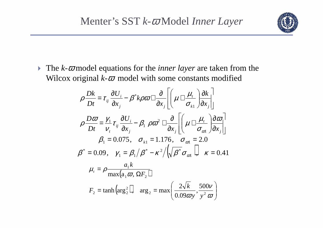
Menter’s SST k-ω Model Inner Layer
The k-ω model equations for the inner layerare taken from the Wilcox original k-ω model with some constants modified
∂∂
+
∂∂+−
∂∂=
∂∂
+
∂∂+−
∂∂=
j
t
jj
iij
t
jk
t
jj
iij
xxx
U
Dt
D
x
k
xk
x
U
Dt
Dk
ωσµµρωβτ
νγωρ
σµµρωβτρ
ω1
21
1
1
*
( ) 41.0,,09.0
0.2,176.1,075.0
1*2*
11*
111
=−==
===
κσβκββγβ
σσβ
ω
ωk
( )
( )
==
Ω=
ων
ω
ωρµ
22222
21
1
500,
09.0
2maxarg,argtanh
,amax
yy
kF
F
kat

Menter’s SST k-ω Model Outer Layer
The k-ω model equations for the outer layerare obtained from by transforming the standard k-ε equations via change-of-variable
Turbulent viscosity computed from:
jj
j
t
jj
iij
t
jk
t
jj
iij
xx
k
xxx
U
Dt
D
x
k
xk
x
U
Dt
Dk
∂∂
∂∂+
∂∂
+
∂∂+−
∂∂=
∂∂
+
∂∂+−
∂∂=
ωω
ρσ
ωσµµρωβτ
νγωρ
σµµρωβτρ
ω
ω
12 2
2
22
2
2
*
( ) 41.0,,09.0
168.1,0.1,0828.0
2*2*
22*
222
=−==
===
κσβκββγβ
σσβ
ω
ωk
ωρµ k
t =

Menter’s SST k-ω Model Blending the Equations
The two sets of equations and the model constants are blended in such a way that the resulting equation set transitions smoothly from one equation to another.
( )
∂∂
∂∂=
=
=
−202
22
2*1
411
10,1
2max
4,
500,maxminarg
argtanh
jjk
k
xx
kCD
yCD
k
yy
k
F
ωω
ρσ
σρων
ωβ
ωω
ω
ω( )
( )γσσβφ
φφφ
ρρ
ω ,,,where
1
1
2111
outer1
inner1
k
FF
Dt
DkF
Dt
DkF
=−+=
⋅⋅⋅+−+
⋅⋅⋅+
layer outler the in
layer inner the in
0
1
1
1
→=
F
F
Wilcox’ original k-ω modelε
εl
23
k=
Wall
k-ω model transformed from std. k-ε model
Modified Wilcox k-ω model

Menter’s SST k-ω Model Blended k-ω Equations
The resulting blended equations are:
Wall
( )jj
j
t
jj
iij
t
jk
t
jj
iij
xx
kF
xxx
U
Dt
D
x
k
xk
x
U
Dt
Dk
∂∂
∂∂−+
∂∂
+
∂∂+−
∂∂=
∂∂
+
∂∂+−
∂∂=
ωω
σρ
ωσµµωρβτ
νγωρ
σµµωρβτρ
ω
ω
112 21
2
*
( ) γσσβφφφφ ω ,,,,1 2111 kFF =−+=

Menter’s SST k-ω Model Turbulent Viscosity
Honors the “structural similarity” constant for boundary layers (Bradshaw, 1967)
Turbulent stress implied by turbulence models can be written as:
In many flow situations (e.g. adverse pressure gradient flows), production of TKE can be much larger than dissipation (Pk >> ε), which leads to predicted turbulent stress larger than what is implied by the structural similarity constant
How can turbulent stress be limited? - A simple trick is to clip turbulent viscosity such that:
ε
Pka
y
U ktt 1ρµµτ =Ω=
∂∂=
1967) (Bradshaw,11 ak
vukavu =
′′−←=′′−≡ ρρτ
kat 1ρµ ≤Ω

Menter’s SST k-ω Model Clippingµt
Turbulent viscosity for the inner layeris computed from:
Remarks F2 is equal to 1 inside boundary layer and goes to zero far from the
wall and free shear layers The name SST (shear-stress transport) is a big word for this simple
trick Note that the vorticity magnitude is used (strain-rate magnitude
could also be used)
( )
( )
magnitude) (vorticityijij
t
yy
kF
F
kak
F
ka
ΩΩ≡Ω
==
Ω=
Ω=
2
500,
09.0
2maxarg,argtanh
,min,amax
22222
2
1
21
1
ων
ω
ωρ
ωρµ

Menter’s SST k-ω Model Submodels & Options
SST k-ω model comes with: Transitional Flowsoption (Off by
default) Compressibility Effectsoption when
ideal-gas option is selected (On by default)
The original SST k-ω model in the literature does not have any of these options These submodels are being borrowed
from Wilcox’ 1998 model - should be used with caution
Do not activate any options to recover the original SST model

k-ω Models Boundary Conditions
Wall boundary conditions The enhanced wall treatment (EWT) is the sole near-wall option for k-ω
models. Neither the standard wall functions option nor the non-equilibrium wall functions option is available for k-ω models in FLUENT 6o The blended laws of the wall are used exclusively
o ω values at wall adjacent cells are computed by blending the wall-limiting value (y->0) and the value in the log-layer
The k-ω models can be used with either a fine near-wall mesh or a coarse near-wall mesh
For other BCs (e.g., inlet, free-stream), the following relationship is used internally, whenever possible, to convert to and from different turbulence quantities:
09.0, ** == βωβε k

Faults in the Boussinesq Assumption
Boussinesq: Rij = 2µtSij
Is simple linear relationship sufficient?o Rij is strongly dependent on flow conditions and history
o Rij changes at rates not entirely related to mean flow processes
Rij is not strictly aligned with Sij for flows with:o sudden changes in mean strain rate
o extra rates of strain (e.g., rapid dilatation, strong streamline curvature)
o rotating fluids
o stress-induced secondary flows
Modifications to two-equation models cannot be generalized for arbitrary flows

0)()( =′+′ ijji uNSuuNSu
Reynolds Stress Models
Starting point is the exact transport equations for the transport of Reynolds stresses, Rij
six transport equations in 3d
Equations are obtained by Reynolds-averaging the product of the exact momentum equations and a fluctuating velocity.
The resulting equations contain several terms that must be modeled

Reynolds Stress Transport Equations
k
ijkijijij
ij
x
JP
Dt
DR
∂∂
+−Φ+= ε
Generation
∂∂+
∂∂
≡k
ikj
k
jkiij x
Uuu
x
UuuP ρ
∂∂
+∂∂′−≡Φ
i
j
j
iij x
u
x
up
k
j
k
iij x
u
x
u
∂∂
∂∂≡ µε 2
Pressure-StrainRedistribution
Dissipation
TurbulentDiffusion
(modeled)
(related to ε)
(modeled)
(computed)
(incompressible flow w/o body forces)
Reynolds StressTransport Eqns.
434214342144 344 21
)( jik
kjiikjjkiijk uux
uuuupupJ∂∂−+′+′≡ µρδδ
Pressure/velocityfluctuations
Turbulenttransport
Moleculartransport
εδε ijij 3
2=
Dissipation Modeling
Dissipation rate is predominantly associated with small scale eddy motions Large scale eddies affected by mean shear
Vortex stretching process breaks eddies down into continually smaller scaleso The directional bias imprinted on turbulence by mean flow is gradually lost
o Small scale eddies assumed to be locally isotropic
o ε is calculated with its own (or related) transport equation
o Compressibility and near-wall anisotropy effects can be accounted for

Turbulent Diffusion
Most closure models combine the pressure diffusion with the triple products and use a simple gradient diffusion hypothesis
Overall performance of models for these terms is generally inconsistent based on isolated comparisons to measured triple products
DNS data indicate that above p′ terms are negligible
( ) ( ) ( )
∂∂
∂∂=
∂∂−++
∂∂
l
jilks
kji
kjikikjkji
k x
uuuu
kC
xuu
xuu
puuu
x ενδδ
ρ'
∂∂
∂∂=
k
ji
k x
uukC
x εσµ
2
Or even a simpler model

Pressure-strain term of same order as production
Pressure-strain term acts to drive turbulence towardsan isotropic state by redistributing the Reynolds stresses
Decomposed into parts
Model of Launder, Reece & Rodi (1978)
∂∂
+∂∂′−≡Φ
i
j
j
iij x
u
x
up
i
j
j
i
i
ji
ii x
u
x
u
x
uu
xx
p
∂∂
∂∂+
∂∂
−=∂∂
′∂21
ρ
∂∂
−
∂∂
+∂∂
+−=Φ ijm
lml
l
ilj
l
jliijij x
Uuu
x
Uuu
x
Uuucbc δ
3
221
i
j
j
i
ii x
U
x
u
xx
p
∂∂
∂∂−=
∂∂′∂
21 2
ρ
“Rapid Part”“Slow” Part
−≡ ijji kuukijb δε
3
2where
wijijijij ,2,1, Φ+Φ+Φ=Φmeangradient
Pressure-Strain Modeling

Pressure-Strain Modeling Options
Wall-reflection effect contains explicit distance from wall
damps the normal stresses perpendicular to wall
enhances stresses parallel to wall
SSG (Speziale, Sarkar and Gatski) Pressure Strain Model Expands the basic LRR model to include non-linear (quadratic) terms
Superior performance demonstrated for some basic shear flowso plane strain, rotating plane shear, axisymmetric expansion/contraction

Characteristics of RSM
Effects of curvature, swirl, and rotation are directly accounted for in the transport equations for the Reynolds stresses. When anisotropy of turbulence significantly affects the mean flow,
consider RSM
More cpu resources (vs. k-ε models) is needed 50-60% more cpu time per iteration and 15-20% additional memory
Strong coupling between Reynolds stresses and the mean flow number of iterations required for convergence may increase
θiu
Heat Transfer
The Reynolds averaging process produces an additional term in the energy equation: Analogous to the Reynolds stresses, this is termed the turbulent heat flux
o It is possible to model a transport equation for the heat flux, but this is not common practice
o Instead, a turbulent thermal diffusivity is defined proportional to the turbulent viscosityThe constant of proportionality is called the turbulent Prandtl number
Generally assumed that Prt ~ 0.85-0.9
Applicable to other scalar transport equations

Turbulence Modeling Options in FLUENT

Topics to be discussed
Near wall modeling options
Low Reynolds number turbulence models
Large Eddy Simulation (LES)

Importance of Near-Wall Turbulence
Walls are main source of vorticity and turbulence
Accurate near-wall modeling is important for most engineering applications Successful prediction of frictional drag for external flows, or pressure
drop for internal flows, depends on fidelity of local wall shear predictions
Pressure drag for bluff bodies is dependent upon extent of separation
Thermal performance of heat exchangers, etc., is determined by wall heat transfer whose prediction depends upon near-wall effects

Near-Wall Modeling Issues
k-ε and RSM models are valid in the turbulent core region and through the log layer Some of the modeled terms in these equations are based on
isotropic behavioro Isotropic diffusion (µt/σ)
o Isotropic dissipation
o Pressure-strain redistribution
o Some model parameters based on experiments of isotropic turbulence
Near-wall flows are anisotropic due to presence of walls
Special near-wall treatments are necessary since equations cannot be integrated down to wall

Flow Behavior in Near-Wall Region
Velocity profile exhibits layer structure identified from dimensional analysis
Inner layer
viscous forces rule, U = f(ρ, τw, µ, y)
Outer layer
dependent upon mean flow
Overlap layer
log-law applies
kU/uτ
Turbulent kinetic energy production and dissipation are nearly equal in the overlap layer
‘turbulent equilibrium’ dissipation >> production in the
viscous sublayer region

In general, ‘wall functions’ are a collection or set of laws that serve as boundary conditions for momentum, energy, and species as well as for turbulence quantities
Wall Function Options The Standard and Non-equilibrium Wall Function options
refer to specific ‘sets’ designed for high Reflows
o The viscosity affected, near-wall region is not resolved
o Near-wall mesh is relatively coarse
o Cell center information bridged by empirically-basedwall functions
Enhanced Wall Treatment or Low-Re Option This near-wall model combines the use of enhancedwall
functions and a two-layer model
o Used for low-Reflows or flows with complex near-wall phenomena
o Generally requires a very fine near-wall mesh capable of resolving the near-wall region
o Turbulence models are modified for ‘inner’ layer
Near-Wall Modeling Options
inner layer
outer layer
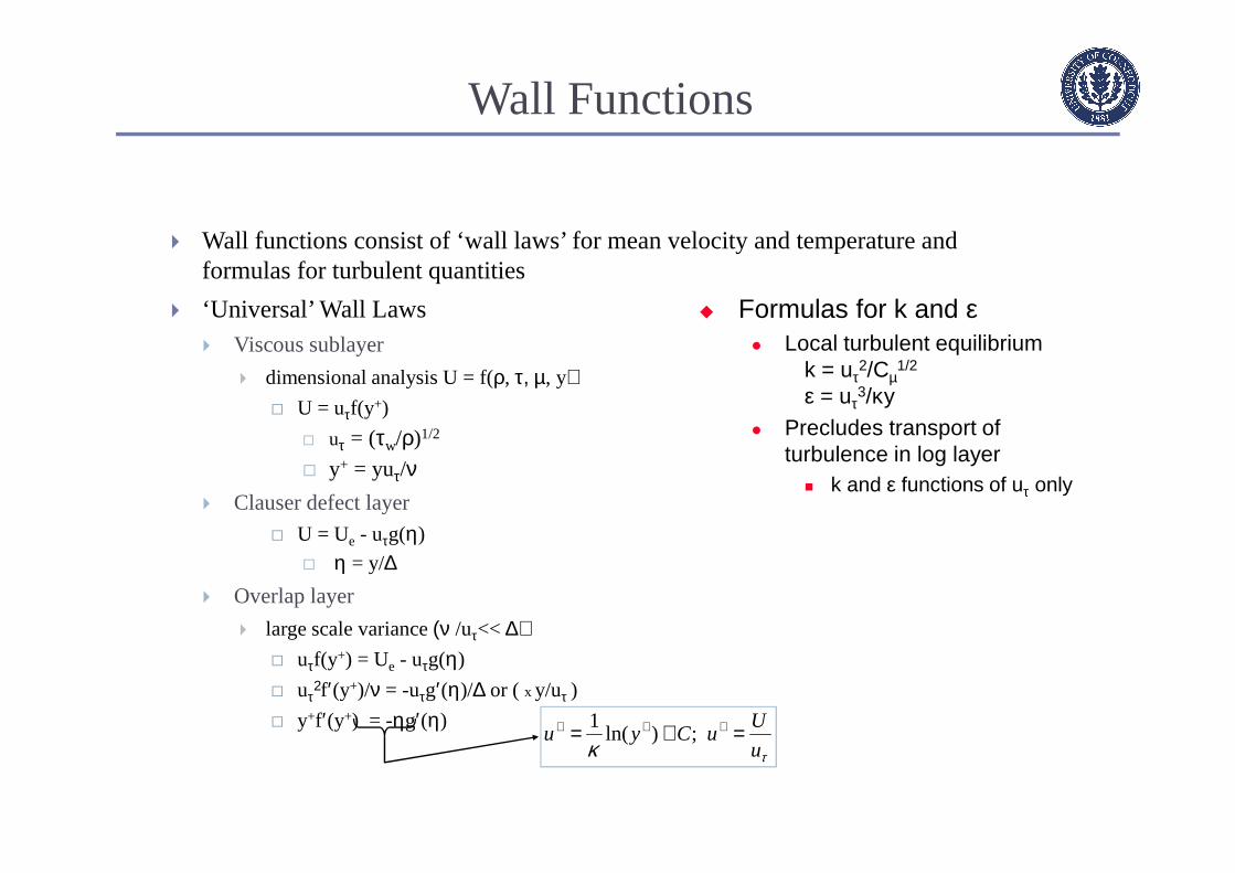
Wall Functions
Wall functions consist of ‘wall laws’ for mean velocity and temperature and formulas for turbulent quantities
‘Universal’ Wall Laws Viscous sublayer
dimensional analysis U = f(ρ, τ, µ, y) U = uτf(y+)
uτ = (τw/ρ)1/2
y+ = yuτ/ν Clauser defect layer
U = Ue - uτg(η)
η = y/∆ Overlap layer
large scale variance (ν /uτ<< ∆) uτf(y+) = Ue - uτg(η)
uτ2f′(y+)/ν = -uτg′(η)/∆ or ( x y/uτ )
y+f′(y+) = -ηg′(η)
τκ u
UuCyu =+= +++ ;)ln(
1
Formulas for k and ε Local turbulent equilibrium
k = uτ2/Cµ
1/2
ε = uτ3/κy
Precludes transport of turbulence in log layer
k and ε functions of uτ only

ρτµ
/
2/14/1
w
PP kCUU ≡∗
µρ µ PP ykC
y2/14/1
≡∗where
∗=∗ EyU ln1
κ
∗=∗ yUfor
**vyy <**vyy >
Standard Wall Functions
Fluent uses Launder-Spalding Wall Functions U = U(ρ, τ, µ, y, k )
o Introduces additional velocity scale for ‘general’ application
o Similar ‘wall laws’ apply for energy and species.
Generally, k is obtained from solution of k transport equationo Cell center is immersed in log layer
o Local equilibrium (production = dissipation) prevails
o ∇∇∇∇k·n = 0 at surface
ε calculated at wall-adjacent cells using local equilibrium assumptiono ε = Cµ
3/4k3/2/κy
Wall functions less reliable when cell intrudes viscous sublayero Forcing (Production = Dissipation) over (Production << Dissipation)

Limitations of Standard Wall Functions
Wall functions become less reliable when flow departs from the conditions assumed in their derivation: Local equilibrium assumption fails
o Severe ∇p
o Transpiration through wall
o strong body forces
o highly 3D flow
o rapidly changing fluid properties near wall
Low-Re flows are pervasive throughout model
Small gaps are present

=
µρ
κρτµµ ykC
EkCU
w
2/14/12/14/1
ln1/
~
+
−+
−=µρκρκy
k
yy
yy
k
ydxdp
UU vv
v
v2
2/12/1ln
21~
where
Rij, k, ε are estimated in each region and used to determine average ε and production of k.
Non-equilibrium Wall Functions
Log-law is sensitized to pressure gradient for better prediction of adverse pressure gradient flows and separation
Relaxed local equilibrium assumptions for TKE in wall-neighboring cells

Enhanced Wall Treatment
Enhanced Wall Treatment Enhanced wall functions
o Momentum boundary condition based on blendedlaw-of-the-wall (Kader)
o Similar blended ‘wall laws’ apply for energy, species, and ωo Kader’s form for blending allows for incorporation of additional physics
Pressure gradient effects
Thermal (including compressibility) effects
Two-layer model
o A blendedtwo-layer model is used to determine near-wall ε field
Domain is divided into viscosity-affected (near-wall) region and turbulent core region
• Based on ‘wall-distance’ turbulent Reynolds number:
• Zoning is dynamic and solution adaptive
High Returbulence model used in outer layer
‘Simple’ turbulence model used in inner layer
o Solutions for ε and µt in each region are blended, e.g.,
The Enhanced Wall Treatment near-wall model is an option for the k-ε and RSM turbulence models
µρ /ykRey ≡
+Γ+Γ+ += turblam ueueu1
( ) ( ) ( )innerouter 1 tt µλµλ εε −+

Two-Layer Zonal Concept
Approach is to divide flow domain into two regions Viscosity affected near-wall region
Fully turbulent core region
Use different turbulence models for each region One-equation (k) near-wall model for the viscosity affected near-wall
region
High-Re k-ε or RSM models for turbulent core region
Wall functions, and their limitations, are avoided

The two regions are demarcated on a cell-by-cell basis: Rey > 200
o turbulent core region
Rey < 200o viscosity affected region
Rey = ρk1/2y/µ y is shortest distance to nearest
wall
zoning is dynamic and solution adaptive
Two-Layer Zones
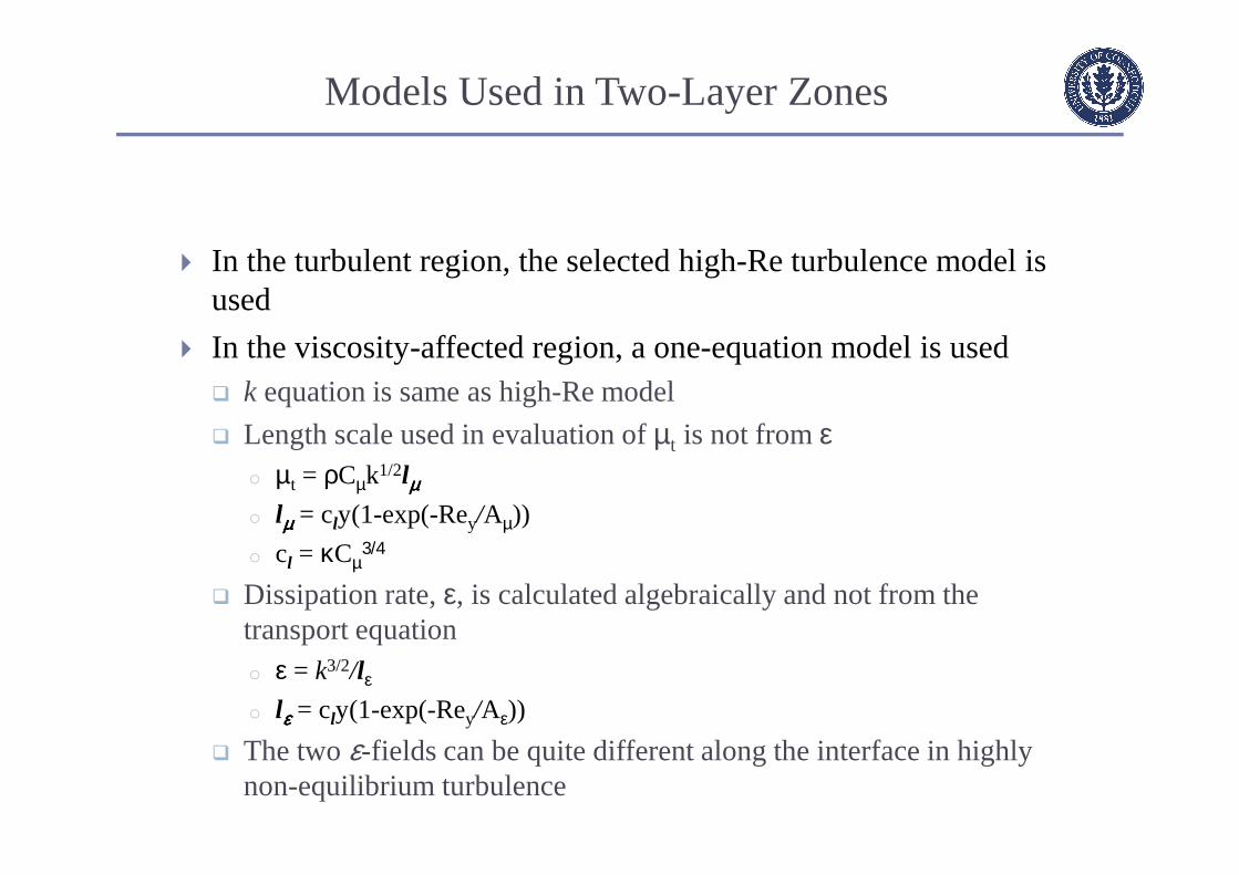
In the turbulent region, the selected high-Re turbulence model is used
In the viscosity-affected region, a one-equation model is used k equation is same as high-Re model
Length scale used in evaluation of µt is not from εo µt = ρCµk1/2lµµµµ
o lµµµµ = cly(1-exp(-Rey/Aµ))
o cl = κCµ3/4
Dissipation rate, ε, is calculated algebraically and not from the transport equationo ε = k3/2/lε
o lεεεε = cly(1-exp(-Rey/Aε))
The two ε-fields can be quite different along the interface in highly non-equilibrium turbulence
Models Used in Two-Layer Zones

Blended ε Equations The transition (of ε-field) from one zone to another can be made
smoother by blending the two sets of ε-equations (Jongen, 1998)
ε
εl
23
k=
Wall
Inner layer
Outer layer ( )Pnb
nbnbPP SaaDt
Dεεεερ =+→⋅⋅⋅= ∑
ε
εl
23
PP
k=
( ) ( )
−+=
=×−+
=+× ∑
A
ReRe
kSaa
*yy
PPP
nbnbnbPP
tanh12
1
123
ε
εεεε
λ
ελεελ
with
l

Blended Turbulent Viscosity
Turbulent viscosity (µt) is also blended using the individual formulations
( ) ( ) ( )
( ) ( )
−−===
−+
µµµµµ
εε
ρµε
ρµ
µλµλ
A
ReyckC
kC y
tt
tt
exp1,,
1
2
lllinnerouter
innerouter
ε
εl
23
k=
Wall
Inner layer
Outer layer ( )ε
ρµ µ
2kCt outer =
( ) µµρµ lkCt =inner

The blending is controlled by two parameters. ( Rey at zonal interface)
Width of blending layer
Zonal Blending Parameters
Wall
Inner layer
Outer layer
98.0tanhyRe
A∆
=
−+=
A
ReRe *yytanh1
2
1ελ
*yRe
default)by (200* =yRe
default)(by 40* =∆ yRe
*yRe∆

Blended Wall Laws
Mean velocity
Blended ‘wall laws’ for temperature and species as well
+Γ+Γ+ += turblam ueueu1
( )++
++
=
=
yEu
yu
turb
lam
ln1
κ
where++ = yulam
( )++ = yEuturb ln1
κ
( )
−′′
==
=+
−=Γ +
+
1exp,5
,01.0,1
4
E
Ec
cb
cayb
ya

‘Wall Law’ Sub-models and Options
“Pressure Gradient Effects” option Always available - deactivated
by default
“Thermal Effects” option Available only when energy
equation is turned on -deactivated by default
Accounts foro Non-adiabatic wall heat transfer
effects
o Compressibility effects - takes effect when ideal-gas option is chosen

Sub-models and Options
The base laws-of-the-wall (mean velocity and temperature) are modified using (White and Christoph, 1972) :
Pressure-gradientcontribution comes from:
Thermal contributions comes from:
21
2
111
−−
+= +++++
+
43421effects thermal
effectsgradient pressure
uuyydy
du γβακ
xd
pd
uy
xd
pd
w
ww
ττναττ ≡+≅ ,
434214434421parameterility compressib
2
parameterfer heat trans
2,,1
2
wp
t
wwp
wtw
TC
u
TC
uquu ττ σγ
τσβγβ
ρρ ≡
′′≡−−≅ ++
+
∂∂
+
∂∂=
jj xxDt
D εσµµερ
ε
t ( )ερµεεε 22
211 CfSCf
k t −
ε−transport equation
turbulent viscosity
ερµ µµ
2
k
Cft =
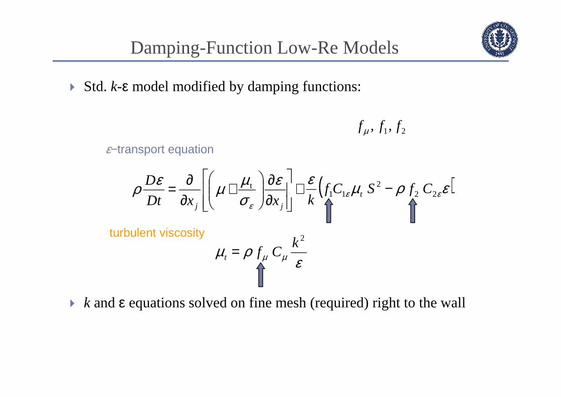
21, , fffµ
Damping-Function Low-Re Models
Std. k-ε model modified by damping functions:
k and ε equations solved on fine mesh (required) right to the wall

Typical Damping Functions Damping functions written in terms of Reynolds numbers:
e.g., Abid’s model:( )
µρµερ
µρ
µερ
εy
Ryk
Rk
R4/1
y
2
t /
e;e;e ===
( )
−
−−=
=
+= −
12exp1
36exp
9
21
1
41)008.0tanh(
2
2
1
4/3
yt
ty
ReRef
f
ReRefµ

Low-Re k-ε Models
Several full low-Re k-ε models now available Lam Bremhorst
Launder-Sharma
Abid
Chang et al.
Abe-Kondo-Nagano
Yang-Shih
Enables modeling of low-Re effects including transitional flows Implementations are problem specific
Features are not visible in GUI Access from TUI

Durbin (1990) suggests that wall normal fluctuations, , are responsible for near-wall transport
behaves quite differently than and attenuation of is a kinematic effect
damping of is a dynamic effect
Model instead of
Requires two additional transport equations: equation for wall-normal fluctuations,
equation for an elliptic relaxation function, f
2 v
2 u2 v 2 w
Tv ~ t2µ kTt ~ µ
2 v2 u
2 v
V2F low-Re k-ε Model

V2F k-ε Model Equations
+
∂∂
+
∂∂=
jj xxDt
D εσµµερ
ε
t ( )ερµ εε 22
1 1
CSCT t −
ε−transport equation
kvfk
x
v
xDt
vD
jkj
ερρσµµρ 2
2t
2
−+
∂∂
+
∂∂=
v2 -transport equation
( )kT
vN
k
SC
k
v
T
C
xx
fLf t
jj
22
2
21
22 1
3
2 −++
−=
∂∂∂−
ρµ
relaxation equation
=
=
εν
εεν
ε η
3
2
322 ,max;6,max C
kCL
kT L
scales

V2F k-ε Model Pros and Cons
Very promising results for a wide range of flow and heat transfer test cases at least as good as the best of the damping function approaches in most
test cases
Still an isotropic eddy-viscosity model Can be extended for RSM
Needs 2 additional equations, so requires more memory and CPU than damping functions

Large Eddy Simulation (LES)
Recall: Two methods can be used to eliminate the need to resolve small scales Reynolds Averaging Approach: Temporal averaging
o All scales are modeled
o Periodic and quasi-periodic unsteady flows
Filtering (LES): Spatial averagingo Transport equations are filtered such that only larger eddies need be
resolved Difficult to model large eddies since they are
• anisotropic
• subject to history effects
• dependent upon flow configuration, boundary conditions, etc.
o Only smaller eddies are modeled Typically isotropic and so more amenable to modeling
o Deterministic unsteadiness of large eddy motions can be resolved

Large Eddy Simulation (LES)
Some applications need explicit computation of unsteady fields Bluff body aerodynamics
Aerodynamically generated noise (sound)
Fluid-structure interaction
Combustion instabilitiy
URANS with good turbulence models can occasionally predict vortex shedding, i.e. largest unsteady scales URANS falls most often short of capturing the remaining large scales
URANS with SST k-w model LES

Energy cascade (Richardson, 1922)
Large Eddy Simulation (LES)

lπ2
E
Energy spectrum against the length scale
( ) ( ) ( )321321 scalesubgrid scaleresolved
ttt ,,, xuxuxu ′+=
( )t,xu
f∆π2
( )t,xu′
LES: Spatial Filtering

A random variable, φ(x), is filtered using a space- filter function, G
With the top-hat filter (among others)
The filtered variable becomes
Most LES codes use implicit filters Filter width determined by grid resolution
∫ ′′′=D
dG xxxxx ),()()( φφ
∈′
=′otherwise 0
for V G
ν ,
xxx
/1)(
V dV
∈′′′= ∫ xxxx ,)(1
)(ν
φφ
LES: Spatial Filtering
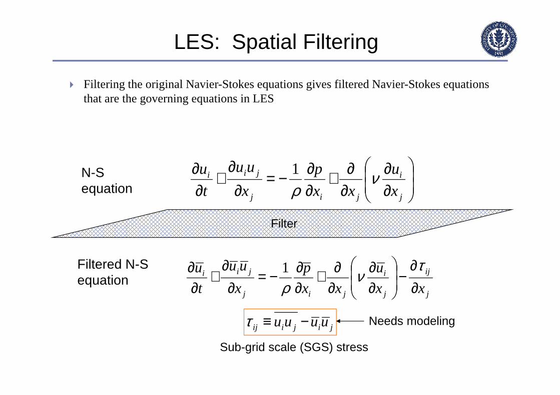
Filtering the original Navier-Stokes equations gives filtered Navier-Stokes equations that are the governing equations in LES
j
ij
j
i
jij
jii
xx
u
xx
p
x
uu
t
u
∂∂
−
∂∂
∂∂+
∂∂−=
∂∂
+∂∂ τ
νρ1
jijiij uuuu −≡τ
∂∂
∂∂+
∂∂−=
∂∂
+∂∂
j
i
jij
jii
x
u
xx
p
x
uu
t
u νρ1N-S
equation
Filtered N-S equation
Needs modeling
Sub-grid scale (SGS) stress
Filter
LES: Spatial Filtering
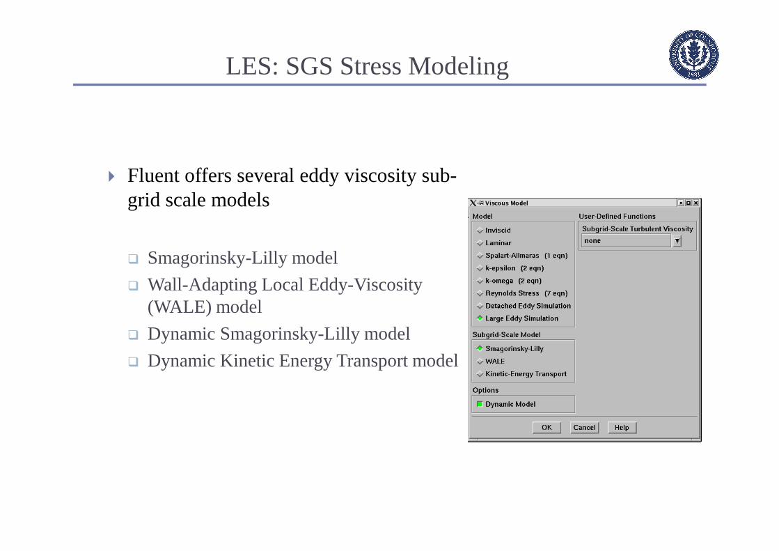
Fluent offers several eddy viscosity sub-grid scale models
Smagorinsky-Lilly model
Wall-Adapting Local Eddy-Viscosity (WALE) model
Dynamic Smagorinsky-Lilly model
Dynamic Kinetic Energy Transport model
LES: SGS Stress Modeling
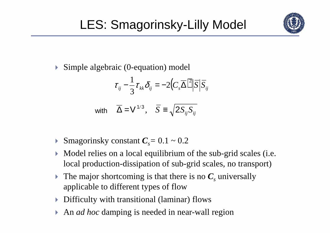
Simple algebraic (0-equation) model
Smagorinsky constant Cs= 0.1 ~ 0.2
Model relies on a local equilibrium of the sub-grid scales (i.e. local production-dissipation of sub-grid scales, no transport)
The major shortcoming is that there is no Cs universally applicable to different types of flow
Difficulty with transitional (laminar) flows
An ad hocdamping is needed in near-wall region
( ) ijsijkkij SSC2
23
1 ∆−=− δττ
ijij SSS 231 ≡=∆ ,/Vwith
LES: Smagorinsky-Lilly Model

Wall-Adapting Local Eddy-Viscosity model
Algebraic (0-equation) model – retains the simplicity of Smagorinsky’smodel
The WALE SGS model adapts to local near-wall flow structure
Wall damping effects are accounted for without using the damping function explicitly
Correct asymptotic behavior of eddy viscosity near wall
Does not allow for non-equilibrium or transport effects for turbulence in sub-grid scales
( ) ( )( ) ( )
444 3444 21onmodificati wall-near
4525
232
//
/
dij
dijijij
dij
dij
sSGSSSSS
SSC
+∆=ν
LES: WALE Model

Based on the similarity concept and Germano’s identity (Germano et al., 1991; Lilly, 1992) Assumes local equilibrium of sub-grid scales, scale similarity
between the smallest resolved scales and the sub-grid scales
The model parameter Cs is automatically adjusted using the resolved velocity field
FLUENT’s implementation Locally dynamic model
Implementd for unstructured meshes (test-filter)
Constant Cs by default clipped at zero and 0.23
Overcomes the shortcomings of the Smagorinsky’s model Can handle transitional flows
The near-wall (damping) effects are accounted for
LES: Dynamic Smagorinsky-Lilly Model

One-equation (for SGS kinetic energy) model. Kim and Menon (1997)
Transport equation for sub-grid scale kinetic energy allows for history and non-equilibrium effects
Like the dynamic Sgamorinsky’s model, the model constants (Ck, Cεεεε) are automatically adjusted on-the-fly using the resolved velocity field
ijsgskijkkij SkC ∆−=− 2/123
1 δττ
∂∂
∂∂+
∆−
∂∂−=
∂∂
+∂
∂
j
sgs
k
sgs
j
sgs
j
iij
j
sgsjsgs
x
k
x
kC
x
u
x
ku
t
k
σν
τ ε
2/3
LES: Dynamic Kinetic Energy Transport Model

LES requires mesh and the time-step sizes sufficiently fine to resolve the energy-containing eddies The cost of resolving near-wall region in high-Re wall-bounded
flows is very high
The mesh resolution determines the fraction of turbulent kinetic energy directly resolved
LES: Grid and Time-Step Size
l
π2ln
Eln
Energy spectrum against the length scale
∆ f
π2ln
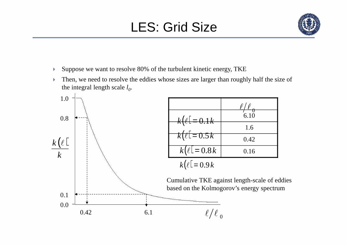
Suppose we want to resolve 80% of the turbulent kinetic energy, TKE
Then, we need to resolve the eddies whose sizes are larger than roughly half the size of the integral length scale l0.
( )k
k l
0ll0.0
1.0
0.1
6.1
0.8 6.10
1.6
0.42
0.16
0ll
( ) kk 1.0=l
( ) kk 5.0=l
( ) kk 8.0=l
Cumulative TKE against length-scale of eddies based on the Kolmogorov’s energy spectrum
0.42
( ) kk 9.0=l
LES: Grid Size

Integral length scale l0 Turbulent kinetic energy peaks at integral length scale. This scale
must be sufficiently resolved
Crude estimation for l0o Based on size of bluff body
o Estimate from correlations
o Perform RANS calculation and compute l0=k1.5/ε
LES: Grid Size
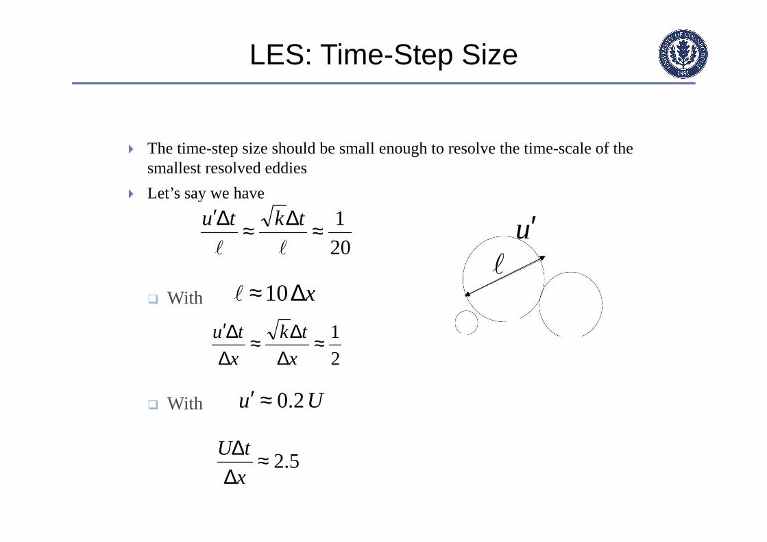
The time-step size should be small enough to resolve the time-scale of the smallest resolved eddies
Let’s say we have
With
With
20
1≈∆≈∆′ll
tktu
l
u′
x∆≈10l
5.2≈∆∆x
tU
Uu 2.0≈′
2
1≈∆
∆≈∆∆′
x
tk
x
tu
LES: Time-Step Size
“Near-wall resolving” approach, y+< 1 All the large scale turbulence is explicitly computed inside the boundary layer down to the
laminar sublayero Resolving the bulk of the energy requires a very fine mesh near the wall. Requires a
relatively fine mesh also in the stream- and span-wise directions
o Turbulence length scale becomes smaller in near-wall region. Too expensive for high-Re wall-bounded flows
“Near-wall modeling” approach – an alternative The near wall turbulence is explicitly calculated inside the boundary layer, but not
necessarily down to the laminar sublayero First grid point can be at y+= 20−150o Instantaneous wall shear stress and instantaneous tangential velocity in the wall adjacent cell
are assumed to be in phase
o Use default or Werner-Wengle (cheaper) wall functions /define/models/viscous/near-wall-treatment/werner-wengle-wall-fn?
o Appropriate for high Reynolds number flows and massively separated flows. Usually fails to predict flows with small separation (adverse pressure gradient induced separation)
Zonal RANS/LES hybrid approaches (e.g., DES)
LES: Grid Size for Wall-Bounded Flows

It is often important to specify a realistic turbulent inflow velocity for accurate prediction of the (downstream) flow
Fluent offers two specification methods for inflow perturbations, available at velocity inlets Spectral synthesizer
Vortex method
( ) ( ) ( )321321randomcoherent
i
averagedtime
ii tuUtu+−
′+= ,, xxx
LES: Inlet Boundary Conditions

Spectral Synthesizer Based on the work of Celik et al.(2001)
Able to synthesize anisotropic, inhomogeneous turbulence from RANS results (k-ε, k-ω, and RSM fields)
The velocity-field satisfies the continuity by design, i.e. it is divergence-free
LES: Inlet Boundary Conditions
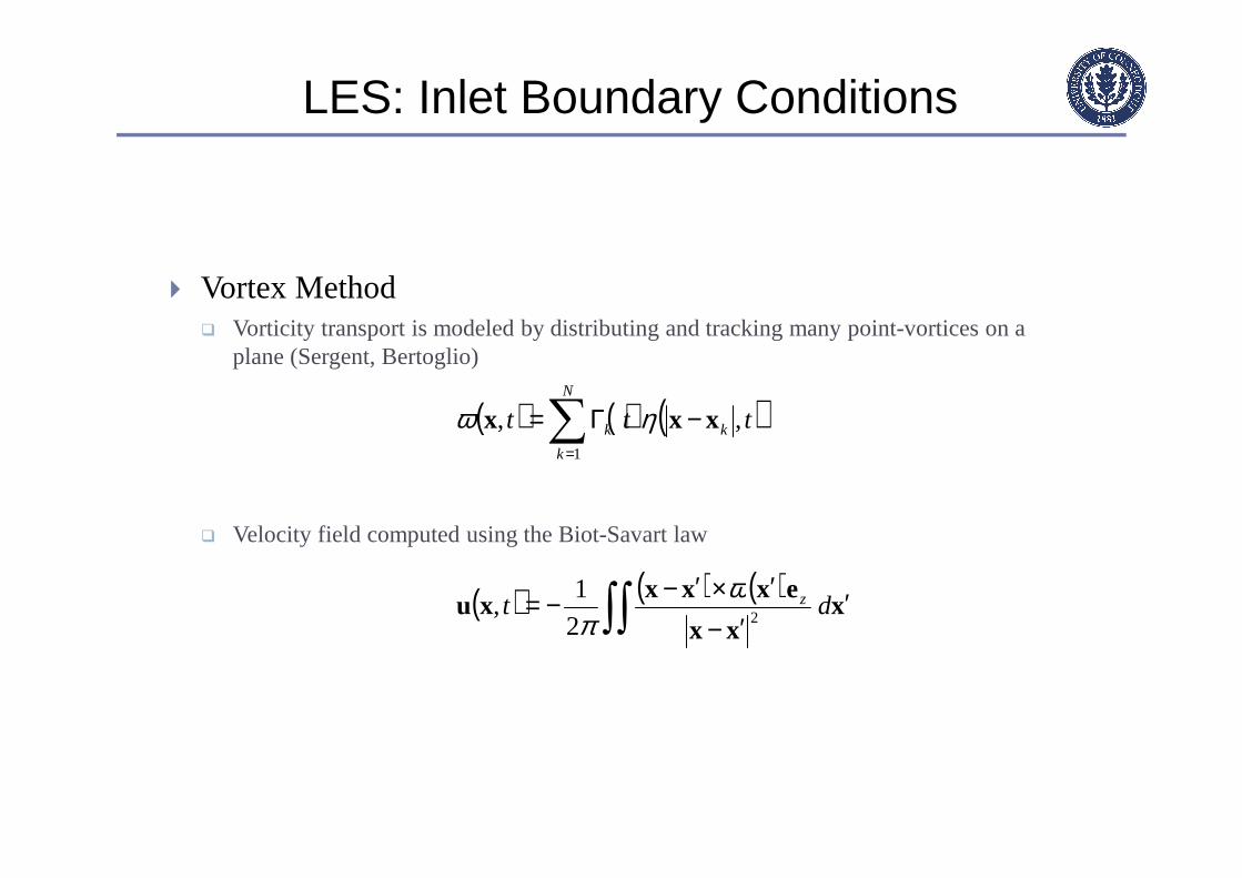
Vortex Method Vorticity transport is modeled by distributing and tracking many point-vortices on a
plane (Sergent, Bertoglio)
Velocity field computed using the Biot-Savart law
( ) ( ) ( )x
xx
exxxxu ′
′−′×′−−= ∫∫ dt z
22
1,
ωπ
( ) ( ) ( )ttt k
N
k
k ,,1
xxx −Γ=∑=
ηω
LES: Inlet Boundary Conditions

Initial condition for velocity field is generally not important for statistically steady-steady flows
Patching a realistic turbulent velocity field can however help shorten the simulation time substantially to get to a statistically steady state
The spectral synthesizer can be used to superimpose turbulence on top of the mean velocity field Velocity field generated by turbulence
synthesizer for homogeneous turbulence
LES: Initial Conditions

CFD Modeling

Is the Flow Turbulent?
External Flows
Internal Flows
Natural Convection
5105×≥xRe along a surface
around an obstacle
where
µρUL
ReL ≡where
Other factors such as free-stream turbulence, surface conditions, and disturbances may cause earlier transition to turbulent flow
L = x, D, Dh, etc.
,3002 ≥hD Re
108 1010 −≥Ra µαρβ 3TLg
Ra∆≡
20,000≥DRe

Choices to be Made
Turbulence Model&
Near-Wall Treatment
Flow Physics
AccuracyRequired
ComputationalResources
TurnaroundTime
Constraints
ComputationalGrid
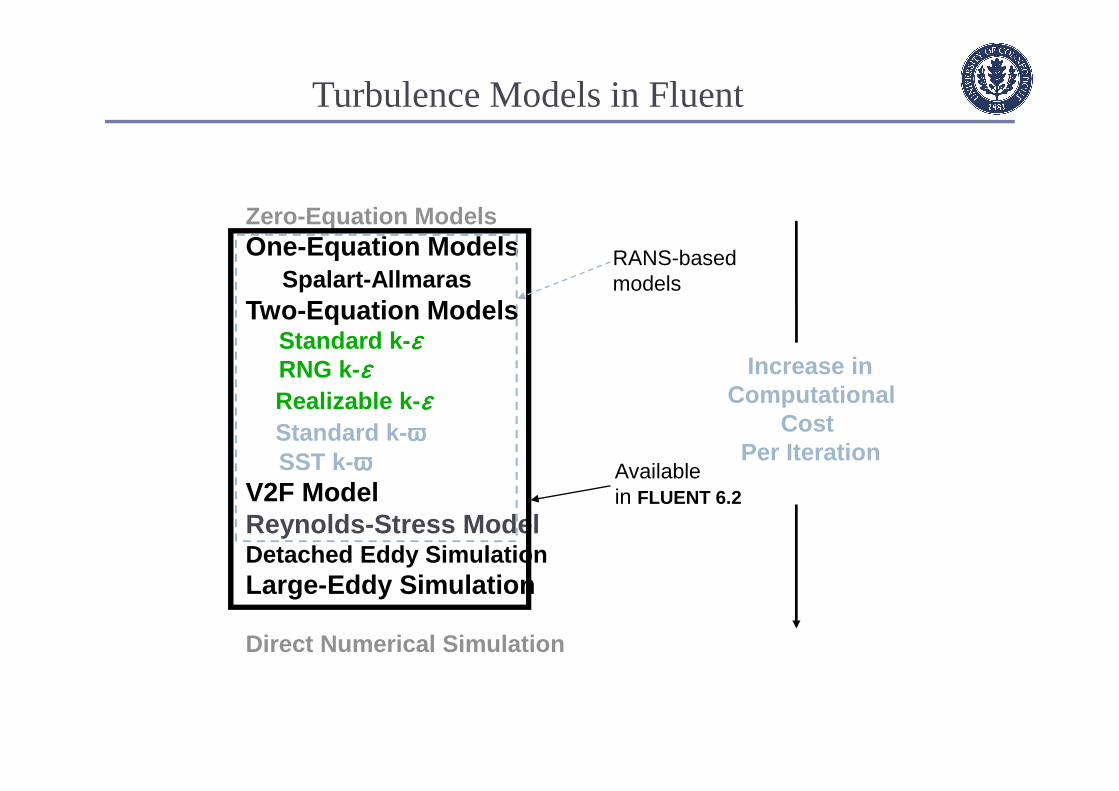
Turbulence Models in Fluent
Zero-Equation ModelsOne-Equation Models
Spalart-AllmarasTwo-Equation Models
Standard k-εεεεRNG k-εεεεRealizable k-εεεεStandard k-ωωωωSST k-ωωωω
V2F ModelReynolds-Stress ModelDetached Eddy SimulationLarge-Eddy Simulation
Direct Numerical Simulation
Increase inComputational
CostPer Iteration
Availablein FLUENT 6.2
RANS-basedmodels

Aspects of Reaction Modeling
Dispersed Phase Models
Droplet/particle dynamicsHeterogeneous reactionDevolatilizationEvaporation Governing Transport
EquationsMassMomentum (turbulence)EnergyChemical Species
Pollutant Models Radiative Heat Transfer Models
Reaction Models
CombustionPremixed, Partially premixed
and Non-premixed
Infinitely Fast ChemistryFinite Rate Chemistry
Surface Reactions

Gas Phase Combustion
Spatio-temporal conservation equations (Navier-Stokes) for Mass (ρ) Momentum (ρυ) Energy (ρh)
Chemical Species (ρYk)
The conservation equations have the general form …
rate of change convection diffusion source
It is useful to quantify energy in terms of enthalpy, defined as ….
chemical thermal
( ) ( ) φφ +
∂∂φ
∂∂=φ
∂∂+φ
∂∂
Sx
Dx
uxt ii
ii
∑ ∫+=species
T
T
pkokk
o
)dTch(Yh

Chemical Kinetics
The k th species mass fraction transport equation is:
Nomenclature: chemical species, denoted Sk , react as:
Example:
( ) ( ) ki
kk
iki
ik R
x
YD
xYu
xY
t+
∂∂ρ
∂∂=ρ
∂∂+ρ
∂∂
∑∑==
ν→νN
1kkk
N
1kkk S"S'
OH2COO2CH 2224 +→+
2"1"0"0"
0'0'2'1'
OHSCOSOSCHS
4321
4321
24232241
=ν=ν=ν=ν=ν=ν=ν=ν
====

Chemical Kinetics
The calculated reaction rate is proportional to the products of the reactant concentrations raised to the power of their respective stoichiometric coefficients.
k th species reaction rate (for a single reaction):
where A = pre-exponential factor
Cj = molar concentration = ρ Yj / Mj
Mk = molecular weight of species k
E = activation energy
R= universal gas constant = 8313 J / kgmol K
β = temperature exponent
Note that for global reactions, , and may be noninteger
∏=
ν−β
ν−ν=
N
1j
'j
RT
E
kkkk
*kCeAT)'"(MR
k*k '' νν ≠

Flames Lengthscale (m)
Velocityscale (m/s)
Reynoldsnumber
Gas turbine combustor 0.1 50 250,000
Fire 5 2 500,000
After-burner 0.5 100 2,500,000
Utility Furnace 10 10 5,000,000
Practical Combustion Processes are Turbulent
Smallest length scale in turbulent flow (called the Kolmogorov scale)
η ∼ L / Re3/4, where L is the combustor characteristic dimension
Number of grid points required for Direct Numerical Simulation (DNS)(resolving all flow scales) ~ (L/ η) 3 = Re 9/4
Example: Re ~ 10 4, number of grid points ~ 10 9
DNS is computationally intractable, and will remain so indefinitely

Necessity for Combustion Modeling
Governing reacting Navier-Stokes equations are accurate,
but DNS is prohibitive ...
Turbulence Large range of time and length scales
Model by time (Reynolds) averagingo Imagine a long exposure photograph of the
visualized flow
o Introduces terms (the Reynolds stresses) which must be modeled
Chemistry Realistic chemical mechanisms have tens of species, hundreds of
reactions, and stiff kinetics (widely disparate time scales)o Determined for a limited number of fuels

Reynolds (Time) Averaged Species Equation
unsteady term convection convection molecular mean
(zero for by mean by turbulent diffusion chemical
steady flows) velocity velocity fluctuations source term
are the k th species mass fraction, diffusion coefficient and chemical source term respectively
Turbulent flux term modeled by mean gradient diffusion as,
, which is consistent in the k-εcontext
Gas phase combustion modeling focuses on Arguably more difficult to model than the Reynolds stresses (turbulence)
( ) ( ) ( ) ki
kk
iki
iki
ik R
x
YD
x"Y"u
xYu
xY
t+
∂∂ρ
∂∂=ρ
∂∂+ρ
∂∂
+ρ
∂∂
kkk R,D,Y
kR
ikttki x/Y/ScY"u" ∂∂⋅= µρ

Turbulence Chemistry Coupling in Flames
( )RTEexpCATRj
jkj −= ∏ νβ
Arrhenius reaction rate terms are highly nonlinear
Cannot neglect the effects of turbulence fluctuations on chemical production rates
)T(RR kk ≠