Embed Size (px)
Citation preview
Clemson UniversityTigerPrints
All Theses Theses
12-2010
A computational method for analysis of materialproperties of a non-pneumatic tire and their effectson static load deflection, vibration and energy lossfrom impact rolling over obstaclesAkshay NarasimhanClemson University, [email protected]
Follow this and additional works at: https://tigerprints.clemson.edu/all_theses
Part of the Mechanical Engineering Commons
This Thesis is brought to you for free and open access by the Theses at TigerPrints. It has been accepted for inclusion in All Theses by an authorizedadministrator of TigerPrints. For more information, please contact [email protected].
Recommended CitationNarasimhan, Akshay, "A computational method for analysis of material properties of a non-pneumatic tire and their effects on staticload deflection, vibration and energy loss from impact rolling over obstacles" (2010). All Theses. 1003.https://tigerprints.clemson.edu/all_theses/1003

A COMPUTATIONAL METHOD FOR ANALYSIS OF MATERIAL
PROPERTIES OF A NON-PNEUMATIC TIRE AND THEIR EFFECTS
ON STATIC LOAD-DEFLECTION, VIBRATION, AND ENERGY
LOSS FROM IMPACT ROLLING OVER OBSTACLES
A Thesis
Presented to
The Graduate School of
Clemson University
In Partial Fulfillment
Of the Requirements for the Degree
Master of Science
Mechanical Engineering
By
Akshay Narasimhan
August 2010
Accepted by:
Dr. Lonny L. Thompson, Committee Chair
Dr. Sherrill Biggers
Dr. John C Ziegert

ii
ABSTRACT
One of the potential sources of vibration during rolling of a non pneumatic tire is
the buckling phenomenon and snapping back of the spokes in tension when they enter
and exit the contact zone. Another source of noise was hypothesized due to a flower
pedal ring vibration effect due to discrete spoke interaction with the ring and contact with
the ground during rolling as the spokes cycle between tension and compression.
Transmission of vibration between the ground force, ring and spokes to the hub was also
considered to be a significant contributor to vibration and noise characteristics of the
Tweel. Previous studies have studied spoke vibration, ground vibration and related
geometrical factors on a two-dimensional (2D) Tweel model. In the present work, a
three-dimensional finite element model of a non-pneumatic tire (Tweel) was considered
which uses a hyperelastic Marlow material model for both ring and spokes based on uni-
axial test data for Polyurethane (PU). Changes in material properties on static load-
deflection curves and vibrations of spoke and ground force reaction during high-speed
rolling are studied. In addition, energy loss upon impact with an obstacle is also studied.
For static load deflection studies, a new analysis procedure is developed which
allows for a cooling step to proceed prior to loading, and yet maintains continuous
contact with the ground. For the dynamic rolling studies, a direct analysis procedure is
developed, where the Tweel is accelerated from rest. This procedure avoids potential
numerical difficulties when defining nonzero initial speeds as used in previous studies.
In order to study the effect of changes in shear modulus for the ring and spokes while
iii
keeping the ratio of volumetric bulk modulus to shear modulus unchanged, the value of
shear modulus is varied from Mooney-Rivlin and Neo-Hookean models obtained from a
least-squares fit of the uni-axial stress-strain data. A total of 6 different material models
are examined together with the original Marlow model. The 6 material models are
divided into 2 sets and each set has 3 levels (unchanged and plus/minus 25% change in
shear modulus).
Upon evaluation of the uniaxial data, the results show that on increasing the shear
modulus, the tangent slope of the normal stress-strain curve increases; whereas with
decreasing shear modulus, the slope decreases. For tensile stresses and strains, the
Mooney-Rivlin best matches the original Marlow material model, compared to the
simpler Neo-Hookean model. However, for large compressive stresses, the Mooney-
Rivlin diverges significantly from the Marlow curve. The simple Neo-Hookean model is
able to fit the Marlow curve better for compression, but is less accurate in tension. As a
result of decreasing shear modulus, the vertical displacement in the static load-deflection
curves increases upon loading. The Neo-Hookean model resulted in decrease in stiffness
when compared to the Mooney-Rivlin and original Marlow model.
The effects of material changes on spoke vibration as measured by changes in
perpendicular distance and vibration in ground interaction measured by FFT frequency
response of vertical reaction force during rolling are also reported. Results show a trend
the vibration decreased when the stiffness of the Mooney Rivlin and the Neo Hookean
models was increased from +25% to -25%. Conversely, the vibration increased when the
stiffness decreased between the extreme limits. However, in several of the material

iv
models for the ring and spokes, the unchanged stiffness gave the lowest vibration
amplitude, suggesting that a optimal value is somewhere between the plus/minus 25%
stiffness limits.
To study energy loss the 3D finite element model of the Tweel is rolled over an
obstacle whose height is 7.5% of the radius of the Tweel. Energy loss is measured by the
reduction in axial hub velocities and kinetic energies (KE) relative to an analytical rigid
wheel with the same mass, moment of inertia and initial velocity. Results show that the
reference Tweel with Marlow material properties, after traversing the obstacle, resulted in
an average reduction in axial velocity and total kinetic energy of only 1.3% and 2.3%,
respectively. Results show that for Mooney Rivlin, a decrease in shear modulus caused a
decrease in energy loss. Conversely, for Neo Hookean, a decrease in shear modulus
resulted in an increase in energy loss and an increase in shear modulus resulted in a
decrease in energy loss.

v
DEDICATION
This thesis is dedicated to my parents, Mr. R. Narasimhan and Mrs. Hemalatha
Narasimhan.
vi
ACKNOWLEDGMENTS
I offer my deepest gratitude to my research advisor Dr. Lonny L. Thompson who
was abundantly helpful and offered invaluable assistance, support and guidance
throughout this research project and for my thesis writing. I attribute the level of my
Masters degree to his encouragement and effort without which this thesis would not have
been completed. I would like to thank Dr. Sherrill Biggers and Dr. John C. Ziegert for
serving on my committee and for their valuable suggestions for improving my thesis.
I would also like to thank Dr. Timothy Rhyne and Mr. Steve Cron of Michelin
and Dr. Andreas Obieglo of BMW for their abundant personal assistance and for
financial support for this research project.
vii
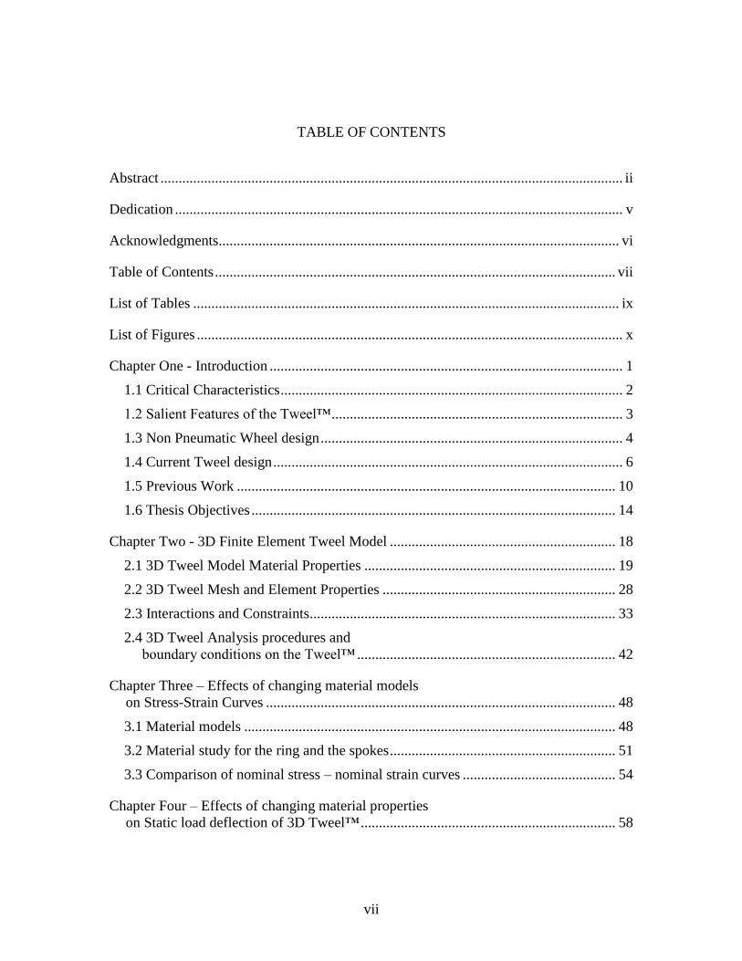
TABLE OF CONTENTS
Abstract ............................................................................................................................... ii
Dedication ........................................................................................................................... v
Acknowledgments.............................................................................................................. vi
Table of Contents .............................................................................................................. vii
List of Tables ..................................................................................................................... ix
List of Figures ..................................................................................................................... x
Chapter One - Introduction ................................................................................................. 1
1.1 Critical Characteristics .............................................................................................. 2
1.2 Salient Features of the Tweel™ ................................................................................ 3
1.3 Non Pneumatic Wheel design ................................................................................... 4
1.4 Current Tweel design ................................................................................................ 6
1.5 Previous Work ........................................................................................................ 10
1.6 Thesis Objectives .................................................................................................... 14
Chapter Two - 3D Finite Element Tweel Model .............................................................. 18
2.1 3D Tweel Model Material Properties ..................................................................... 19
2.2 3D Tweel Mesh and Element Properties ................................................................ 28
2.3 Interactions and Constraints .................................................................................... 33
2.4 3D Tweel Analysis procedures and
boundary conditions on the Tweel™ ....................................................................... 42
Chapter Three – Effects of changing material models
on Stress-Strain Curves ................................................................................................ 48
3.1 Material models ...................................................................................................... 48
3.2 Material study for the ring and the spokes .............................................................. 51
3.3 Comparison of nominal stress – nominal strain curves .......................................... 54
Chapter Four – Effects of changing material properties
on Static load deflection of 3D Tweel™ ...................................................................... 58
viii
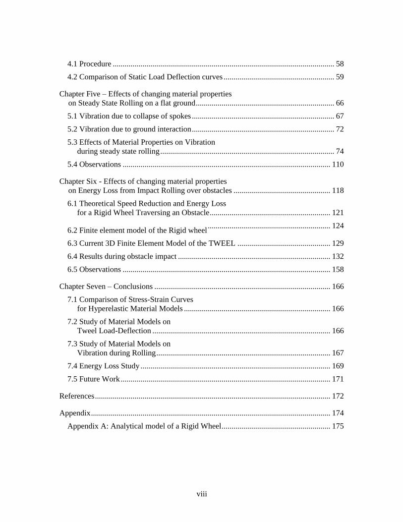
4.1 Procedure ................................................................................................................ 58
4.2 Comparison of Static Load Deflection curves ........................................................ 59
Chapter Five – Effects of changing material properties
on Steady State Rolling on a flat ground ...................................................................... 66
5.1 Vibration due to collapse of spokes ........................................................................ 67
5.2 Vibration due to ground interaction ........................................................................ 72
5.3 Effects of Material Properties on Vibration
during steady state rolling ........................................................................................ 74
5.4 Observations ......................................................................................................... 110
Chapter Six - Effects of changing material properties
on Energy Loss from Impact Rolling over obstacles ................................................. 118
6.1 Theoretical Speed Reduction and Energy Loss
for a Rigid Wheel Traversing an Obstacle ............................................................. 121
6.2 Finite element model of the Rigid wheel .............................................................. 124
6.3 Current 3D Finite Element Model of the TWEEL ............................................... 129
6.4 Results during obstacle impact ............................................................................. 132
6.5 Observations ......................................................................................................... 158
Chapter Seven – Conclusions ......................................................................................... 166
7.1 Comparison of Stress-Strain Curves
for Hyperelastic Material Models .......................................................................... 166
7.2 Study of Material Models on
Tweel Load-Deflection .......................................................................................... 166
7.3 Study of Material Models on
Vibration during Rolling ........................................................................................ 167
7.4 Energy Loss Study ................................................................................................ 169
7.5 Future Work .......................................................................................................... 171
References ....................................................................................................................... 172
Appendix ......................................................................................................................... 174
Appendix A: Analytical model of a Rigid Wheel ....................................................... 175
ix
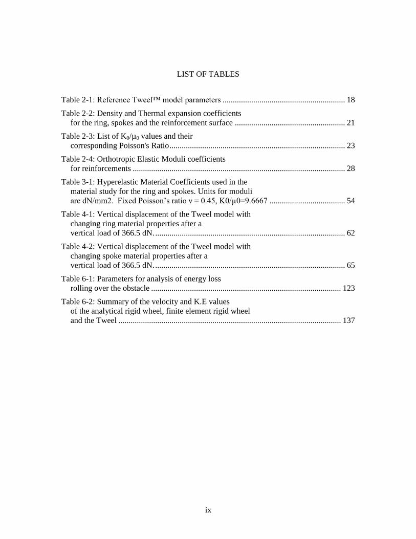
LIST OF TABLES
Table 2-1: Reference Tweel™ model parameters ............................................................ 18
Table 2-2: Density and Thermal expansion coefficients
for the ring, spokes and the reinforcement surface ...................................................... 21
Table 2-3: List of K0/µ0 values and their
corresponding Poisson's Ratio ...................................................................................... 23
Table 2-4: Orthotropic Elastic Moduli coefficients
for reinforcements ........................................................................................................ 28
Table 3-1: Hyperelastic Material Coefficients used in the
material study for the ring and spokes. Units for moduli
are dN/mm2. Fixed Poisson‟s ratio ν = 0.45, K0/µ0=9.6667 ..................................... 54
Table 4-1: Vertical displacement of the Tweel model with
changing ring material properties after a
vertical load of 366.5 dN. ............................................................................................. 62
Table 4-2: Vertical displacement of the Tweel model with
changing spoke material properties after a
vertical load of 366.5 dN. ............................................................................................. 65
Table 6-1: Parameters for analysis of energy loss
rolling over the obstacle ............................................................................................. 123
Table 6-2: Summary of the velocity and K.E values
of the analytical rigid wheel, finite element rigid wheel
and the Tweel ............................................................................................................. 137
x
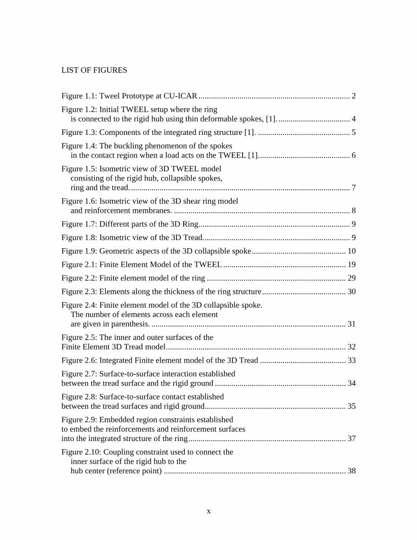
LIST OF FIGURES
Figure 1.1: Tweel Prototype at CU-ICAR .......................................................................... 2
Figure 1.2: Initial TWEEL setup where the ring
is connected to the rigid hub using thin deformable spokes, [1]. ................................... 4
Figure 1.3: Components of the integrated ring structure [1]. ............................................. 5
Figure 1.4: The buckling phenomenon of the spokes
in the contact region when a load acts on the TWEEL [1]. ............................................ 6
Figure 1.5: Isometric view of 3D TWEEL model
consisting of the rigid hub, collapsible spokes,
ring and the tread. ........................................................................................................... 7
Figure 1.6: Isometric view of the 3D shear ring model
and reinforcement membranes. ...................................................................................... 8
Figure 1.7: Different parts of the 3D Ring .......................................................................... 9
Figure 1.8: Isometric view of the 3D Tread. ....................................................................... 9
Figure 1.9: Geometric aspects of the 3D collapsible spoke .............................................. 10
Figure 2.1: Finite Element Model of the TWEEL ............................................................ 19
Figure 2.2: Finite element model of the ring .................................................................... 29
Figure 2.3: Elements along the thickness of the ring structure ......................................... 30
Figure 2.4: Finite element model of the 3D collapsible spoke.
The number of elements across each element
are given in parenthesis. ............................................................................................... 31
Figure 2.5: The inner and outer surfaces of the
Finite Element 3D Tread model ........................................................................................ 32
Figure 2.6: Integrated Finite element model of the 3D Tread .......................................... 33
Figure 2.7: Surface-to-surface interaction established
between the tread surface and the rigid ground ................................................................ 34
Figure 2.8: Surface-to-surface contact established
between the tread surfaces and rigid ground..................................................................... 35
Figure 2.9: Embedded region constraints established
to embed the reinforcements and reinforcement surfaces
into the integrated structure of the ring ............................................................................. 37
Figure 2.10: Coupling constraint used to connect the
inner surface of the rigid hub to the
hub center (reference point) ......................................................................................... 38

xi
Figure 2.11: Tie constraint to tie the outer surface of the
rigid hub and the interfacing spoke surfaces ................................................................ 39
Figure 2.12: Tie constraint to tie the interfacing spoke surfaces
and the inner surface of the inner coverage of the ring ................................................ 40
Figure 2.13: Tie constraint to tie the outer surface of the
outer coverage and the tread ......................................................................................... 41
Figure 2.14: Tie constraint to tie the two inner surfaces
of the half treads ........................................................................................................... 42
Figure 2.15: Boundary conditions imposed on the
Tweel during static load deflection procedure ............................................................. 44
Figure 2.16: Boundary conditions imposed on the
Tweel during loading, accelerating and cooling (step 1)
in procedures 2 and 3 .................................................................................................... 47
Figure 3.1: Comparison of the nominal stress – nominal strain
curves for the Marlow, Mooney Rivlin and Neo Hookean
strain energy potential models fitted to the Marlow data. ............................................ 55
Figure 3.2: Comparison of nominal stress – nominal strain
curves of the original fitted, reduced and increased modulus
Mooney Rivlin material models. .................................................................................. 56
Figure 3.3: Comparison of nominal stress – nominal strain
curves of the original fitted, reduced and increased modulus
Mooney Rivlin material models. .................................................................................. 57
Figure 4.1: Fully compressed Tweel upon the action
of applied load at the hub center .................................................................................. 58
Figure 4.2: Comparison of load deflection curves for Marlow,
and fitted Mooney Rivlin and Neo Hookean material models for
the ring. Properties for the spokes are not changed. ..................................................... 60
Figure 4.3: Comparison of load deflection curves for
different Mooney Rivlin models for the ring.
Properties for spoke are not changed. .......................................................................... 61
Figure 4.4: Comparison of load deflection curves for
different Neo Hookean models for the ring.
Properties of spokes are not changed. .......................................................................... 62
Figure 4.5: Comparison of load deflection curves for Marlow,
fitted Mooney Rivlin and Neo Hookean material models
for the spokes. Ring properties are not changed. ........................................................ 63

xii
Figure 4.6: Comparison of load deflection curves for
different Mooney-Rivlin models for the spoke.
Ring properties are not changed. .................................................................................. 64
Figure 4.7: Comparison of load deflection curves for
different Neo Hookean models for the spoke.
Ring properties are not changed. .................................................................................. 65
Figure 5.1: Vertical marker nodes involved in the
calculation perpendicular distance of spoke marker nodes
from virtual plane of spoke .......................................................................................... 68
Figure 5.2: Vertical spoke marker nodes in both
initial and deformed geometries of the Tweel .............................................................. 69
Figure 5.3: Perpendicular distance of the vertical
spoke marker nodes from the plane of spoke ............................................................... 70
Figure 5.4: Magnitude of FFT with hamming window
for perpendicular distance for middle vertical node. .................................................... 71
Figure 5.5: Reaction force exerted by the ground on the Tweel ....................................... 72
Figure 5.6: FFT amplitude for the ground reaction force ................................................. 73
Figure 5.7: Perpendicular distance of spoke marker nodes
from plane of spoke. ..................................................................................................... 74
Figure 5.8: Magnitude of FFT amplitude of
perpendicular distance for middle node. ...................................................................... 75
Figure 5.9: Ground Reaction force ................................................................................... 76
Figure 5.10: FFT amplitude for the ground reaction force ............................................... 76
Figure 5.11: Perpendicular distance of vertical
marker nodes from plane of spoke ............................................................................... 77
Figure 5.12: Magnitude of FFT amplitude of
perpendicular distance for the middle node ................................................................. 78
Figure 5.13: Ground reaction force ................................................................................... 79
Figure 5.14: FFT amplitude for ground reaction force ..................................................... 79
Figure 5.15: Perpendicular distance of vertical
marker nodes from plane of spoke ............................................................................... 80
Figure 5.16: Magnitude of FFT amplitudes of
perpendicular distance for the middle node ................................................................. 81
Figure 5.17: Reaction force exerted by the ground on the Tweel ..................................... 82
Figure 5.18: Magnitude of FFT amplitudes
for ground reaction force .............................................................................................. 83

xiii
Figure 5.19: Perpendicular distance of vertical
spoke marker nodes from plane of spoke ..................................................................... 84
Figure 5.20: Magnitude of FFT amplitudes of
perpendicular distance for the middle node ................................................................. 84
Figure 5.21: Ground reaction force ................................................................................... 85
Figure 5.22: Magnitude of FFT amplitudes
for ground reaction force .............................................................................................. 86
Figure 5.23: Perpendicular distance of vertical
spoke marker nodes from plane of spoke ..................................................................... 87
Figure 5.24: Magnitude of FFT amplitudes of
perpendicular distance for middle node ....................................................................... 87
Figure 5.25: Reaction force exerted by
the ground on the Tweel ............................................................................................... 88
Figure 5.26: Magnitude of FFT amplitudes
for ground reaction force .............................................................................................. 89
Figure 5.27: Perpendicular distance of spoke
marker nodes from plane of spoke ............................................................................... 90
Figure 5.28: Magnitude of FFT amplitudes of
perpendicular distance for middle node ....................................................................... 90
Figure 5.29: Ground reaction force ................................................................................... 91
Figure 5.30: Magnitude of FFT amplitudes for
ground reaction force .................................................................................................... 92
Figure 5.31: Perpendicular distance of vertical
marker nodes from plane of spoke ............................................................................... 93
Figure 5.32: Magnitude of FFT amplitudes of
perpendicular distance for the middle node ................................................................. 93
Figure 5.33: Ground reaction force ................................................................................... 94
Figure 5.34: Magnitude of FFT amplitude
for ground reaction force .............................................................................................. 95
Figure 5.35: Perpendicular distance for vertical
spoke marker nodes from plane of spoke ......................................................................... 96
Figure 5.36: Magnitude of FFT amplitudes of
perpendicular distance for middle node ....................................................................... 96
Figure 5.37: Reaction force exerted by the ground on the Tweel ..................................... 97
Figure 5.38: Magnitude of FFT amplitudes
for ground reaction force .............................................................................................. 98
xiv
Figure 5.39: Perpendicular distance of the vertical
spoke marker nodes from the plane of spoke ............................................................... 99
Figure 5.40: Magnitude of FFT amplitudes of
perpendicular distance for the middle node ................................................................. 99
Figure 5.41: Ground reaction force ................................................................................. 100
Figure 5.42: Magnitude of FFT amplitudes
for ground reaction force ............................................................................................ 101
Figure 5.43: Perpendicular distance of vertical
spoke marker nodes from the plane of spoke ............................................................. 102
Figure 5.44: Magnitude of FFT amplitudes of the
perpendicular distance for the middle spoke .............................................................. 102
Figure 5.45: Reaction force exerted by
the ground on the Tweel ............................................................................................. 103
Figure 5.46: Magnitude of FFT amplitudes
for ground reaction force ............................................................................................ 104
Figure 5.47: Perpendicular distance of the
vertical marker nodes from plane of spoke ................................................................ 105
Figure 5.48: Magnitude of FFT amplitudes of
perpendicular distance for the middle node ............................................................... 105
Figure 5.49: Ground reaction force ................................................................................. 106
Figure 5.50: Magnitude of FFT amplitudes
for ground reaction force ............................................................................................ 107
Figure 5.51: Perpendicular distance of the
vertical spoke marker nodes ............................................................................................ 108
Figure 5.52: magnitude of FFT amplitudes of
perpendicular distance for the middle node
on the spoke edge ....................................................................................................... 108
Figure 5.53: Reaction force exerted by
the ground on the Tweel ............................................................................................. 109
Figure 5.54: Magnitude of FFT amplitudes
for ground reaction force. ........................................................................................... 110
Figure 5.55: RMS of FFT amplitudes of
perpendicular distance from virtual spoke
plane for reference and unchanged models ................................................................ 111
Figure 5.56: RMS of FFT amplitudes for
different Mooney Rivlin and Neo Hookean models .................................................. 112
xv
Figure 5.57: RMS of FFT amplitudes of
ground reaction force for reference and unchanged models ...................................... 115
Figure 5.58: RMS of FFT amplitudes for different
Mooney Rivlin and Neo Hookean models ................................................................. 116
Figure 6.1: Rigid Wheel traversing an obstacle. ............................................................. 119
Figure 6.2: Horizontal velocity profile for the
rigid wheel and the pneumatic wheel from [1, 14] ..................................................... 119
Figure 6.3: Horizontal velocity profile for the
pneumatic wheel and the Tweel from [1, 14] ............................................................. 120
Figure 6.4: Finite element model of the rigid wheel ....................................................... 125
Figure 6.5: Enforcement of a kinematic coupling constraint
to model rigid hub. ..................................................................................................... 125
Figure 6.6: Comparison of the axial hub velocity of the
finite element rigid wheel model based on a steel ring
with the analytical model. .......................................................................................... 127
Figure 6.7: Comparison of the kinetic energy of the
finite element rigid wheel model with the analytical model. ..................................... 127
Figure 6.8: The different energies for the finite element steel ring
with rigid hub model of the rigid wheel ..................................................................... 129
Figure 6.9: Analysis set up for Tweel rolling over
rigid obstacle of height b = 0.074 R. .......................................................................... 131
Figure 6.10: Analysis set up of the 3D Tweel
finite element model rolling over an obstacle ............................................................ 131
Figure 6.11: XY view of the Finite Element model setup .............................................. 132
Figure 6.12: Deformation of the Tread upon
impacting the obstacle ................................................................................................ 133
Figure 6.13: X-Y view of 3D Tweel impacting an obstacle ........................................... 133
Figure 6.14: Deformation of the spokes and the tread
upon first obstacle impact. .......................................................................................... 134
Figure 6.15: Deformation of the spokes and the tread
upon impact with the ground after traversing the obstacle. ....................................... 134
Figure 6.16: The axial hub velocity of the TWEEL
in comparison with the rigid wheel. ........................................................................... 135
Figure 6.17: Kinetic energy of the TWEEL
in comparison with the Rigid wheel. .......................................................................... 136

xvi
Figure 6.18: Vertical hub velocity profile of
the Reference Marlow model ..................................................................................... 138
Figure 6.19: Rotational velocity profile of
the Reference Marlow model. .................................................................................... 138
Figure 6.20: Axial hub velocity profiles of the
Tweel with Marlow properties (1.265%) and an
unchanged Mooney Rivlin material model
for the ring (1.22%) .................................................................................................... 139
Figure 6.21: Kinetic Energy profiles for the
Tweel with Marlow properties (2.345%) and an
unchanged Mooney Rivlin material model
for the ring (2.337%) .................................................................................................. 140
Figure 6.22: Axial hub velocity profiles of the
Tweel with a reduced Mooney Rivlin model
for the ring (1.093%)
and an unchanged Mooney Rivlin material model
for the ring (1.22%) .................................................................................................... 141
Figure 6.23: Kinetic Energy profiles for the
Tweel with a reduced Mooney Rivlin material model
(2.1075%) and an unchanged Mooney Rivlin material model
for the ring (2.3375%) ................................................................................................ 142
Figure 6.24: Axial hub velocity profiles of the
Tweel with an increased Mooney Rivlin model
for the ring (1.368%) and an unchanged Mooney Rivlin
material model for the ring (1.22%) ........................................................................... 143
Figure 6.25: Kinetic Energy profiles for the
Tweel with a reduced Mooney Rivlin material model
(2.4813%) and an unchanged Mooney Rivlin material model
for the ring (2.3375%) ................................................................................................ 144
Figure 6.26: Axial hub velocity profiles of the
Tweel with an unchanged Neo Hookean model
for the ring (1.314%) and the reference model (1.265%) .......................................... 145
Figure 6.27: Kinetic Energy profiles for the
Tweel with an unchanged Neo Hookean material model
(2.5423%) and the reference model (2.3457%) ......................................................... 145
Figure 6.28: Axial hub velocity profiles of the
Tweel with an unchanged Neo Hookean model for the ring
(1.314%) and a reduced Neo Hookean model (1.87%) .............................................. 146

xvii
Figure 6.29: Kinetic Energy profiles for the
Tweel with an unchanged Neo Hookean material model
(2.5423%) and a reduced Neo Hookean model (3.3278%) ........................................ 147
Figure 6.30: Axial hub velocity profiles of the
Tweel with an unchanged Neo Hookean model
for the ring (1.314%) and an increased Neo Hookean
model (1.139%) .......................................................................................................... 148
Figure 6.31: Kinetic Energy profiles for the Tweel
with an unchanged Neo Hookean material model
(2.5423%) and an increased Neo Hookean model (2.2448%) ................................... 148
Figure 6.32: Axial hub velocity profile of the
Tweel with Mooney Rivlin unchanged model on
the spokes (1.32%) and with Marlow properties (1.265%) ........................................ 149
Figure 6.33: Kinetic energy profiles for the
Tweel with Mooney Rivlin for the spokes (2.5258%)
and with Marlow properties (2.3457%) ..................................................................... 150
Figure 6.34: Axial hub velocity profile for the
Tweel with a Mooney Rivlin unchanged model (1.32%)
and a Mooney Rivlin reduced model (1.034%) ......................................................... 151
Figure 6.35: Kinetic energy profile for the
Tweel with a Mooney Rivlin unchanged model (2.5258%)
and a Mooney Rivlin reduced model (1.9594%) ....................................................... 151
Figure 6.36: Axial hub velocity profiles for the
Tweel with a Mooney Rivlin unchanged model (1.32%)
and a Mooney Rivlin increased model (1.338%) ....................................................... 152
Figure 6.37: Kinetic energy profiles for the
Tweel with a Mooney Rivlin unchanged model (2.5258%)
and a Mooney Rivlin increased model (2.4796%) for the spokes .............................. 153
Figure 6.38: Axial hub velocity profile for the
Tweel model with a Neo Hookean unchanged model
(1.28%) and with Marlow properties (1.265%) ......................................................... 154
Figure 6.39: Kinetic energy profile for the
Tweel with a Neo Hookean unchanged model
(2.3511%) and Marlow properties (2.3457%) ............................................................ 154
Figure 6.40: Axial hub velocity profile for the
Tweel model with a Neo Hookean unchanged model
(1.28%) and a Neo Hookean reduced model (2 %) .................................................... 155
xviii
Figure 6.41: Kinetic energy profile for the
Tweel with a Neo Hookean unchanged model
(2.3511%) and Neo Hookean reduced model (3.6457%) .......................................... 156
Figure 6.42: Axial hub velocity profile for the
Tweel with a Neo Hookean unchanged model
(1.28%) and a Neo Hookean increased model (0.958%) ........................................... 157
Figure 6.43: Kinetic energy profiles for the
Tweel with a Neo Hookean unchanged model
(23.3135%) and a Neo Hookean increased model (23.7025%) ................................. 157
Figure 6.44: Reduction in axial hub velocity of the
Tweel with a Mooney Rivlin unchanged model,
Neo Hookean unchanged model and Marlow properties. .......................................... 158
Figure 6.45: Comparison of reduction in axial hub
velocities for different levels of Mooney Rivlin
and Neo Hookean material models ............................................................................ 160
Figure 6.46: Percentage of proportion of energy
lost for a Mooney Rivlin unchanged model,
Neo Hookean unchanged model and Marlow properties ........................................... 162
Figure 6.47: Percentage difference of the Kinetic energy
values between the different Tweel models
and the analytical rigid wheel ..................................................................................... 164

1
CHAPTER ONE - INTRODUCTION
John Boyd Dunlop developed the pneumatic wheel in the late 18th
century. The
importance of the pneumatic wheel was realized when it was rolled along with a rigid
wheel on a rough terrain paved with cobble stones. During impacts with obstacles, the
pneumatic wheel was at an advantageous position than the rigid wheel due to different
characteristics. These are termed as the critical characteristics of the pneumatic wheel and
are discussed in detail in [1].
Over the years, constant efforts have been made to improve the design of the
pneumatic wheel. However, even the current design of the pneumatic wheel has its
disadvantages such as inflation loss from punctures, regular maintenance to keep correct
air pressure and durability. In addition, with different constraints imposed on the current
design of the pneumatic wheel, there is no optimal design till date. These constraints are
explained in [1]. As a solution to these prevailing problems, a non-pneumatic wheel
design called a Tweel was proposed by Michelin Engineers, T. B. Rhyne and S. M. Cron.
This design not only possesses the critical characteristics of the pneumatic wheel, but also
expands the limited design space provided by the pneumatic wheel [1]. A prototype
Tweel used for testing at Michelin and the Clemson University International Center for
Automotive Research (CU-ICAR) is shown in Figure 1.1.

2
Figure 1.1: Tweel Prototype at CU-ICAR
1.1 Critical Characteristics
The pneumatic tire possesses four important characteristics. These characteristics
were recognized from the behavior when impacting obstacles [1] and used to design the
structure of the Tweel.
1. Low contact pressure for the non pneumatic wheel was achieved by replacing
the inflation pressure with a circular beam which deforms primarily in shear.
This beam is comprised of two in-extensible membranes separated by a
relatively low elastic modulus material layer.
2. Low stiffness for the non pneumatic wheel was proposed by connecting the
elastic layer to the hub using thin deformable elastic spokes.
3
3. Low mass for the non pneumatic wheel is achieved by having the same
structure as the bicycle wheel (invention of the tensioned spokes). This is
explained in detail [1].
4. Finally, the most important characteristic, low energy loss from impacting
obstacles is achieved by designing a Tweel with similar mass, moment of
inertia as the pneumatic tire. When rolling with the same initial velocity over
an obstacle, it was observed that the Tweel loses less energy compared to the
pneumatic wheel.
1.2 Salient Features of the Tweel™
It has been explained in [1] that the non-pneumatic Tweel possesses the critical
characteristics seen in the pneumatic wheel. These characteristics compliment the design
of the non-pneumatic wheel, thereby increasing the design space and eliminating many
constraints.
The contact pressure and the vertical stiffness of the non pneumatic wheel are
decoupled unlike the pneumatic structure where they are interdependent. In this new
proposed structure, combinations like high contact pressure / low stiffness and low
contact pressure / high stiffness can be achieved.
The stiffness curve for the non pneumatic wheel can be adjusted according to the
design requirements. On the other hand, the pneumatic wheel always acts like a slightly
hardening spring.
With the shear beam replacing the inflation pressure, it eliminates the need for an
enclosed space to hold the compressed gas and also saves a lot of weight. The shear beam
also eliminates the need for maintaining optimal inflation pressure
4
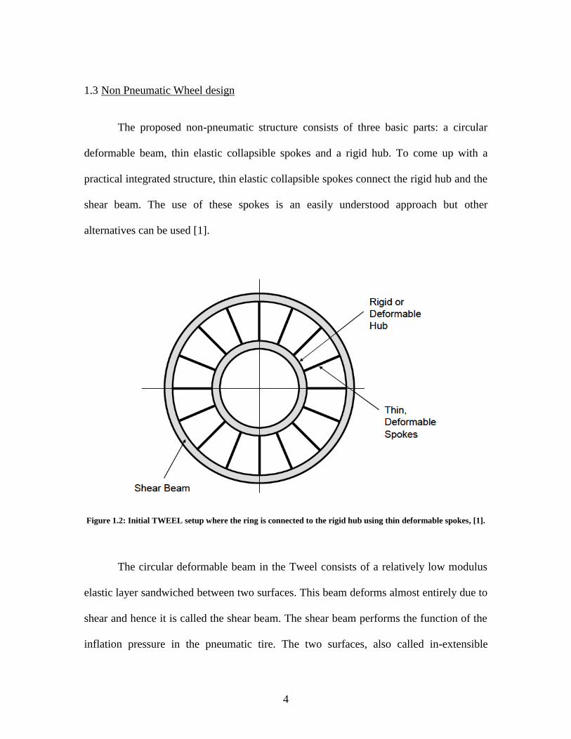
1.3 Non Pneumatic Wheel design
The proposed non-pneumatic structure consists of three basic parts: a circular
deformable beam, thin elastic collapsible spokes and a rigid hub. To come up with a
practical integrated structure, thin elastic collapsible spokes connect the rigid hub and the
shear beam. The use of these spokes is an easily understood approach but other
alternatives can be used [1].
Figure 1.2: Initial TWEEL setup where the ring is connected to the rigid hub using thin deformable spokes, [1].
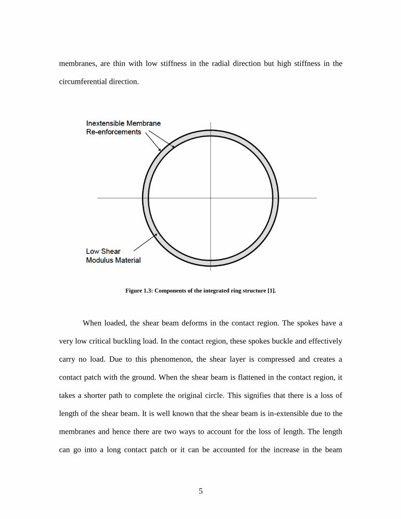
The circular deformable beam in the Tweel consists of a relatively low modulus
elastic layer sandwiched between two surfaces. This beam deforms almost entirely due to
shear and hence it is called the shear beam. The shear beam performs the function of the
inflation pressure in the pneumatic tire. The two surfaces, also called in-extensible
5
membranes, are thin with low stiffness in the radial direction but high stiffness in the
circumferential direction.
Figure 1.3: Components of the integrated ring structure [1].
When loaded, the shear beam deforms in the contact region. The spokes have a
very low critical buckling load. In the contact region, these spokes buckle and effectively
carry no load. Due to this phenomenon, the shear layer is compressed and creates a
contact patch with the ground. When the shear beam is flattened in the contact region, it
takes a shorter path to complete the original circle. This signifies that there is a loss of
length of the shear beam. It is well known that the shear beam is in-extensible due to the
membranes and hence there are two ways to account for the loss of length. The length
can go into a long contact patch or it can be accounted for the increase in the beam
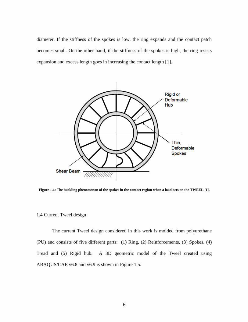
6
diameter. If the stiffness of the spokes is low, the ring expands and the contact patch
becomes small. On the other hand, if the stiffness of the spokes is high, the ring resists
expansion and excess length goes in increasing the contact length [1].
Figure 1.4: The buckling phenomenon of the spokes in the contact region when a load acts on the TWEEL [1].
1.4 Current Tweel design
The current Tweel design considered in this work is molded from polyurethane
(PU) and consists of five different parts: (1) Ring, (2) Reinforcements, (3) Spokes, (4)
Tread and (5) Rigid hub. A 3D geometric model of the Tweel created using
ABAQUS/CAE v6.8 and v6.9 is shown in Figure 1.5.

7
Figure 1.5: Isometric view of 3D TWEEL model consisting of the rigid hub, collapsible spokes, ring and the
tread.
The ring is a composite structure consisting of a shear beam and in-extensible
membranes. These membranes are embedded inside the ring structure. These in-
extensible membranes are also called reinforcements due to the high stiffness and
strength of these membranes in the circumferential direction. The number of
reinforcements in the shear ring varies by design but a minimum of two is required to
form the shear beam behavior. The reinforcements flank the shear beam on either side
thereby dividing the ring into number of layers depending on their number. In this work,
the Tweel is designed for the BMW Mini Cooper with specified dimensions for the
Ring with
shear layer
and
reinforcements
Collapsible spokes
Rigid or
deformable
hub
Tread

8
outside diameter and hub diameter and uses two reinforcement membranes in the shear
ring, see Figure 1.6.
Figure 1.6: Isometric view of the 3D shear ring model and reinforcement membranes.
As stated, the Mini Cooper Tweel has 2 in-extensible membranes flanking the
shear beam and hence divides the ring into three layers; the shear layer and outer and
inner coverage. The reinforcement that is situated nearer to the hub center is called the
inner reinforcement. The other reinforcement is called the outer reinforcement. Also, the
section of the ring above the inner reinforcement is called the inner coverage while the
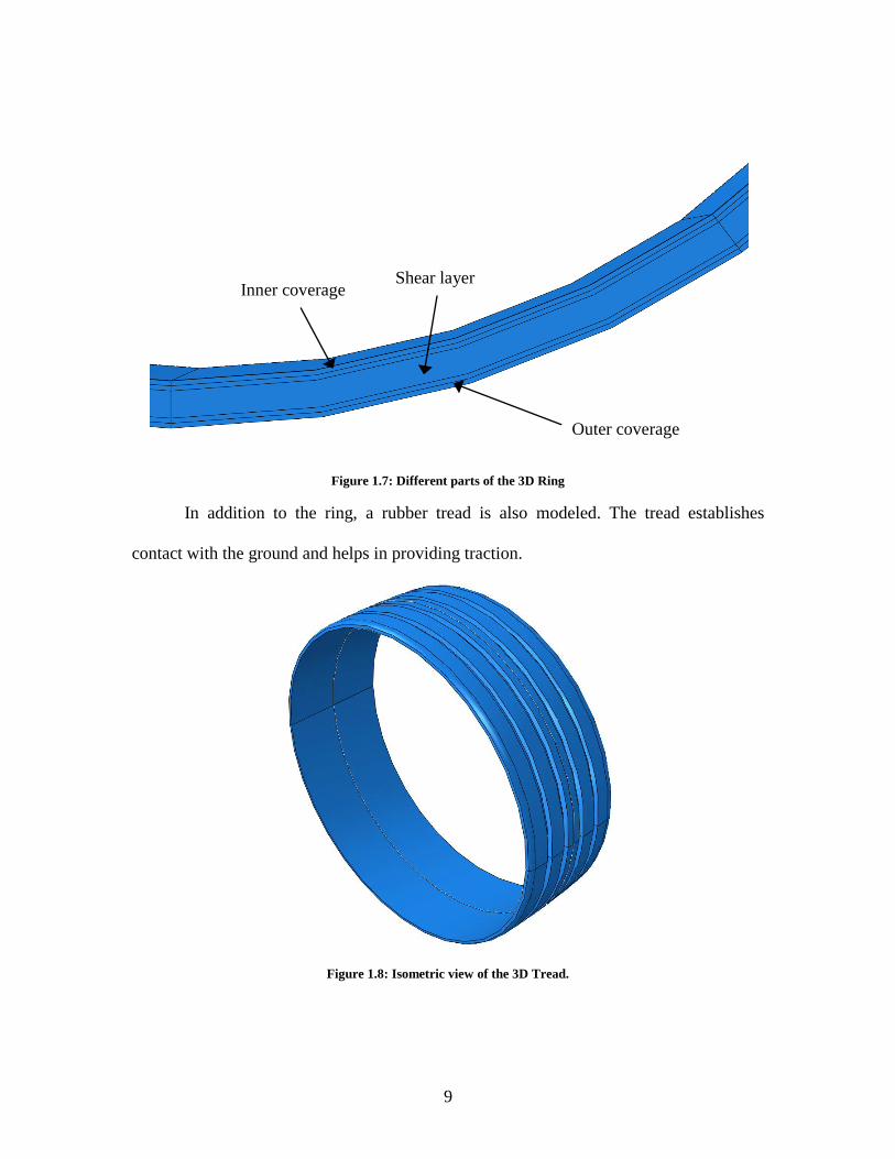
section of the ring below the shear beam is called the outer coverage; see Figure 1.7.
9
Figure 1.7: Different parts of the 3D Ring
In addition to the ring, a rubber tread is also modeled. The tread establishes
contact with the ground and helps in providing traction.
Figure 1.8: Isometric view of the 3D Tread.
Inner coverage Shear layer
Outer coverage
10
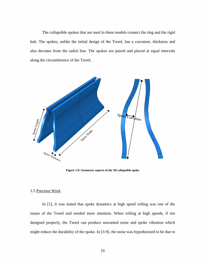
The collapsible spokes that are used in these models connect the ring and the rigid
hub. The spokes, unlike the initial design of the Tweel, has a curvature, thickness and
also deviates from the radial line. The spokes are paired and placed at equal intervals
along the circumference of the Tweel.
Figure 1.9: Geometric aspects of the 3D collapsible spoke
1.5 Previous Work
In [1], it was stated that spoke dynamics at high speed rolling was one of the
issues of the Tweel and needed more attention. When rolling at high speeds, if not
designed properly, the Tweel can produce unwanted noise and spoke vibration which
might reduce the durability of the spoke. In [3-9], the noise was hypothesized to be due to

11
the buckling phenomenon of the spoke when entering and leaving the contact zone and
the resulting vibration during the tension phase of the spoke as it passes around the top
portion of the rotating wheel. In [10] another source of noise was hypothesized due to a
flower pedal ring vibration effect due to discrete spoke interaction with the ring and
contact with the ground during rolling as the spokes cycle between tension and
compression. Transmission of vibration between the ground force, ring and spokes to the
hub was also considered to be a significant contributor to vibration and noise
characteristics of the Tweel.
In [2], spoke dynamics was investigated by analyzing a single 3D spoke in
ABAQUS. The 3D spoke was tied to point (hub center) using different connector
elements and was rotated. A 3% static tensile strain was imposed on the spoke and was
then accelerated to a speed of 80 km/hr. This is equivalent to simulating a Tweel rolling
at a high speed over a rigid surface.
The research work in [3] involved the development of a computational procedure
for simulating high speed rolling of a Tweel in contact with a rigid plane. In addition, the
spoke vibration frequencies were monitored and the spoke length vs. time profile was
obtained. This served as an input boundary condition for a 3D Tweel spoke to capture in-
plane and out-of-plane vibrations. From the computational procedure, it was concluded
that the spoke vibrations were not significantly affected by the thickness of the spoke.
From the 3D spoke analysis, significant out-of-plane vibrations were captured which
were not present in the 2D Tweel models.
12
In the research work of [4], changes were made to modeling techniques to
accurately represent the cooling and loading phases during steady state rolling using
ABAQUS/Explicit. In addition, the single 3D spoke was analyzed under high speed
rolling conditions. From this analysis was concluded that scalloping the edges of the
spoke drastically reduced the vibration amplitude but did not have a strong effect on the
dominant frequency. An optimal amount of scalloping was suggested.
In [5], important spoke and ring (geometric) parameters were considered for
vibration and were studied using Taguchi‟s Robust Parameter Design and orthogonal
arrays. To evaluate every combination, set of output parameters such as perpendicular
distance of the spoke from a virtual plane, ground reaction forces due to vibration of the
Tweel and ring vibration were monitored and compared. Increasing spoke curvature and
decreasing spoke length resulted in decreasing the magnitude of the output parameters.
In the research work of [6], a systematic study of the effects of spoke angle
deviations from radial lines (DeRad) was performed using Taguchi‟s Robust Parameter
Design Method and Orthogonal Arrays. Also, effects of a new alternate spoke pair
concept wherein every other pair has same thickness, curvature, or combinations of both
were examined. It was concluded that DeRad did not affect the spoke and ground
vibration as much as spoke curvature and spoke length. On comparing with a reference
model having uniform spoke thickness, the alternating spoke pair model with plus/minus
5% difference in thickness between the odd and the even spoke resulted in reducing the
RMS and maximum amplitudes, and also spread out the excitation frequencies of the
ground force reaction.

13
In [7], more importance was given to other parameters of the Tweel although the
spoke thickness and spoke curvature were the most influencing parameters. Also, an
additional L8 orthogonal array with variables of shear beam thickness, inner coverage,
and outer coverage, leaving appropriate columns open to expose interactions between the
ring variables was created. All key geometric variables were combined and included the
effects of uncontrollable factors of rolling speed and ground pushup in a Robust
Parametric Design study. For a complete study, a L27 orthogonal array was proposed with
combinations of 9 geometric design parameters considered as control factors with three
levels each. It was concluded that the Tweel stiffness is dominated by the change in
spoke thickness as compared to the change in number of spoke pairs. Spoke curvature
was concluded to be the most important parameter which influenced ground and spoke
vibration. Strong interactions were found between the ring variables such as shear beam,
inner and outer reinforcements.
In the computational studies in [3,4], the analysis procedure consisted of an
nonzero initial condition followed by a ground and hub center motion. This allowed for a
steady-state rolling condition with constant speed (zero acceleration) to be achieved
without starting from rest and accelerating up to steady speed, resulting in significantly
reduced compute time. In [5,6,7], a different analysis procedure is used with the same
goal of starting the analysis with an initial nonzero speed. While these procedures give
effective results for studying steady-state rolling, they do not allow for the possibility of a
ground which includes obstacles. In addition, all of the full Tweel rolling models used
previously where 2D planar models which are approximations to the physical 3D Tweel

14
structure. While many of the geometric features of the Tweel are planar and projected in
the width dimension to form a 3D structure, some components are not entirely planar,
such as the spokes and tread which have a taper across the width dimension. In addition,
the grooves in the tread can only be captured in a 3D model of the Tweel.
1.6 Thesis Objectives
In this work, the computational procedure is expanded to a complete 3D model of
the Tweel including a detailed model of the 3D geometry of the spokes and tread. Since
the model is 3D, the idealized orthotropic properties of the reinforcements in the 2D
planar model, are treated more accurately with 3D geometric effects. In addition, a major
goal of this work is to investigate energy loss due to Tweel impact over obstacles; a new
analysis procedure is developed. In this procedure, rolling is started from rest and
accelerated to steady speed and then held constant prior to impacting ground obstacles.
For efficiency, the static load is applied during the acceleration step prior to reaching a
steady speed. History outputs of hub velocity and kinetic energy are also reported. The
flat ground surface also had to be modified to model the shape of a typical obstacle, and a
friction model between the ground and wheel tread contact was also utilized.
For static load deflection studies, a new analysis procedure is developed which allows for
a cooling step to proceed prior to loading, and yet maintains continuous contact with the
ground.
In addition to the study of energy loss, another objective was to study spoke
vibration and ground force vibration during steady rolling without any assumptions or
potential artificial numerical artifacts due to approximations of nonzero initial speed in

15
the Abaqus model. The benefit of starting the simulation from rest in the new analysis
procedure, allows for vibration results during rolling which should better compare to
physical experiments. Since the analysis steps start from rest, the total time required by
the solver to fully accelerate to the desired steady speed is greater than previous studies
using approximate nonzero startup procedures. As a result, the analysis requires
significant CPU processing time. To solve this problem, all analysis are performed on
the Clemson Palmetto computer cluster, with multiple processors and compute cores in a
highly paralyzed environment facilitated by Abaqus/Explicit finite element software.
Both geometric and material properties play an important role in the performance
of tires. In previous work, geometric factors were studied on the vibration of spokes and
ground force interaction of a rolling non-pneumatic tire. In this present work, material
factors are considered. Changes in material properties on static load-deflection curves,
energy loss rolling over obstacles, and vibrations of spoke and ground force reaction
during rolling are studied. For this study, a 3D finite element model of a non-pneumatic
tire was considered which uses a Hyperelastic Marlow material model for both ring and
spokes based on uni-axial test data for Polyurethane (PU). In order to study the effect of
changes in shear modulus for the ring and spokes while keeping the ratio of volumetric
bulk modulus to shear modulus unchanged, the value of shear modulus is varied from
Mooney-Rivlin and Neo-Hookean models obtained from a least-squares fit of the uni-
axial stress-strain data. A total of 6 different material models are examined together with
the original Marlow model. The 6 material models are divided into 2 sets and each set has
3 levels (unchanged and plus/minus 25% change in shear modulus). In addition to static
16
load-deflection curves which are important for vehicle design integration, the effects of
material changes on spoke vibration as measured by changes in perpendicular distance
and vibration in ground interaction measured by FFT frequency response of vertical
reaction force during rolling are also reported.
Another goal is to compute the energy loss of the current 3D Tweel model as it
traverses an obstacle. In this work, a computational procedure is developed to study the
effects of changes in shear modulus on Kinetic energy loss during impact over obstacles.
Reduction in Kinetic energy and velocity after traversing an obstacle results in a smaller
change in linear momentum, implying reduced linear impulse, which in turn leads to
reduced harshness over rough surfaces. Results of the 3D Tweel model are compared
with a rigid wheel finite element model having the same mass, outside radius, and
moment of inertia as that of the Tweel. An analytical model of the rigid wheel with a
simplified analysis of the obstacle is also developed and is compared with FEA models of
both the Tweel and rigid wheel.
An outline of the thesis is as follows.
In Chapter 2, details of the material and geometric features of the 3D Finite
Element Tweel model are described, including mesh and element properties and
interactions and constraints. At the end of this chapter, the new analysis procedure from
rolling starting from rest is given.
In Chapter 3, a comparison of stress-strain curves for the PU material and
hyperelastic models with different shear modulus is given.

17
In Chapter 4, the effects of shear modulus on the slope and magnitude static load
vs. displacement curves are studied. The slope of these curves gives a measure of the
vertical stiffness of the Tweel which is a key design variable for vehicle integration.
In Chapter 5, vibration due to steady-state rolling on a flat ground is studied.
Measures of vibration include changes in perpendicular distance from a virtual plane of a
spoke, and ground force interaction. Vibration amplitudes and frequencies are quantified
using Fast Fourier Transform (FFT) response of the time-dependent signals during
rolling.
In Chapter 6, results for energy loss during rolling over an obstacle are reported
and compared.
Finally, in Chapter 7, conclusions are made and suggestions are given for future work.

18
CHAPTER TWO - 3D FINITE ELEMENT TWEEL MODEL
In previous works [3-10], the Tweel™ model was a 2D planar model generated
using a Abaqus/CAE plug-in and Python scripts. As discussed earlier, in this work a 3D
Tweel model is used. The original 3D geometric model was constructed by Steve Cron at
Michelin [11]. The finite element mesh and materials in this 3D model are modified for
studies of the shear modulus in the PU material in the ring and spokes. Different element
types are defined for the static and dynamic/explicit analysis performed in this work. In
addition, a new analysis step procedure was developed to allow rolling from rest and the
ground was recreated to construct obstacles for energy loss studies. The geometric
dimensions of the 3D Tweel that are used for analysis purposes are given in Table 2-1.
The geometric model of the 3D Tweel is shown in Figure 2.1.
Table 2-1: Reference Tweel™ model parameters
Parameters Reference Tweel Model
Outside Diameter 584 mm
Inside Diameter 422 mm
Tread Thickness 5 mm
Ring Thickness 15 mm
Outside Coverage 8.3 mm
Inside Coverage 3 mm
Number of Spoke Pairs 25
Spoke Thickness 4.2 mm
Spoke Curvature 8 mm

19
Figure 2.1: Finite Element Model of the TWEEL
2.1 3D Tweel Model Material Properties
The 3D Tweel model consists of two different materials; Isotropic Hyperelastic
materials for the ring, spokes, reinforcement surface and tread, and Orthotropic Elastic
material for the reinforcements.
Hyperelastic materials are isotropic, nonlinear and show instantaneous elastic
responses up to large strain values. On the other hand, elastic materials are valid for only
small elastic strains and can be isotropic or orthotropic. Depending on the number of
20
symmetry planes passing through every point, an elastic material can be classified into
isotropic, anisotropic and orthotropic. Symmetry planes refer to the number of axes of
rotational symmetry. Isotropic material has infinite number of symmetry planes whereas
an orthotropic material has two or three orthogonal symmetry planes. Hence, the
mechanical properties for orthotropic materials vary in different directions [13].
The default/reference 3D model has Hyperelastic Marlow uni-axial stress-strain
properties for the shear beam, reinforcement surface and collapsible spokes. The same
properties are used for the shear beam and spokes to model the Polyurathane (PU), while
the reinforcement surface has different properties.
2.1.1 Isotropic Hyperelastic material for the shear beam, collapsible spokes, tread and
reinforcement surface
The materials for the shear beam collapsible spokes are modeled with an Isotropic
Hyperelastic model. The constitutive behavior of a Hyperelastic material is defined based
on a stress-total strain relationship. These materials are very often considered to be
incompressible [12]. In this work, three different material models have been used for
measuring spoke vibration, ground reaction force and strains on the spokes.
The Marlow properties are defined by the experimental stress-strain test data
provided by Michelin. The density of the material is given in daN.sec2/mm
4 and the
thermal expansion coefficient is defined in /o
C. As mentioned earlier, the Marlow
properties are the same for both the shear beam (ring) and the collapsible spokes but are
different for the reinforcement surface. The mass density and thermal expansion
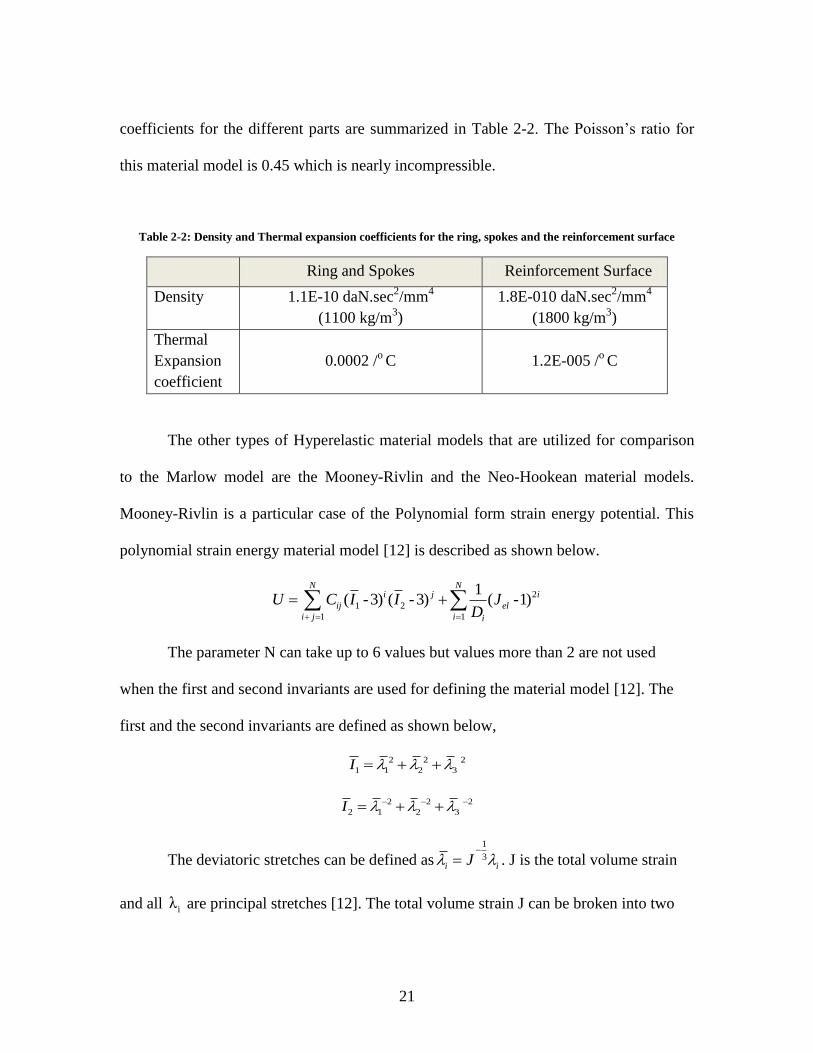
21
coefficients for the different parts are summarized in Table 2-2. The Poisson‟s ratio for
this material model is 0.45 which is nearly incompressible.
Table 2-2: Density and Thermal expansion coefficients for the ring, spokes and the reinforcement surface
Ring and Spokes Reinforcement Surface
Density 1.1E-10 daN.sec2/mm
4
(1100 kg/m3)
1.8E-010 daN.sec2/mm
4
(1800 kg/m3)
Thermal
Expansion
coefficient
0.0002 /o C 1.2E-005 /
o C
The other types of Hyperelastic material models that are utilized for comparison
to the Marlow model are the Mooney-Rivlin and the Neo-Hookean material models.
Mooney-Rivlin is a particular case of the Polynomial form strain energy potential. This
polynomial strain energy material model [12] is described as shown below.
2
1 2
1 1
1( -3) ( -3) ( -1)
N Ni j i
ij el
i j i i
U C I I JD
The parameter N can take up to 6 values but values more than 2 are not used
when the first and second invariants are used for defining the material model [12]. The
first and the second invariants are defined as shown below,
2 2 2
1 1 2 3I
2 2 2
2 1 2 3I
The deviatoric stretches can be defined as1
3i iJ
. J is the total volume strain
and all iλ are principal stretches [12]. The total volume strain J can be broken into two

22
components namely Jel and J
th. The following relation can be established to define the
total volume strain,
el
th
JJ
J
Jth
follows from the linear thermal expansion,
3(1 )th
thJ ,
where thε depends on the temperature and isotropic thermal expansion coefficient.
th th T
The Di values relate to compressibility of the model. If all Di are zero, then the
model is fully incompressible. If D1 is zero, all other Di should be zero. The D values are
related to the initial bulk modulus of the material model K0. Similarly, the values of Cij
are related to the initial shear modulus of the material model µ0.
For the material to be consistent with linear elasticity in the limit of small strains,
it is necessary for the initial moduli to be defined as,
0 10 012( )C C
0
1
2K
D
where 0 is the initial shear modulus and K0 is the initial bulk modulus. The shear
modulus controls the material distortion, whereas the bulk modulus controls the volume
change. For Hyperelastic materials, the relative compressibility of a material can be
determined from the ratio of the initial bulk modulus over the initial shear modulus, i.e.

23
K0 /0. These coefficients, in the form of a ratio can be related to the Poisson‟s ratio by
the formula,
0 0
0 0
3 2
6 2
K
K
Using this relation, numerous material models can be derived for a fixed
Poisson‟s ratio and/or the ratio between initial shear and bulk modulus. A few values for
the relative compressibility to distortion ratio and its corresponding Poisson‟s ratio are
given below in Table 2-3.
Table 2-3: List of K0/µ0 values and their corresponding Poisson's Ratio
K0/µ0 υ
10 0.452
20 0.475
50 0.49
100 0.495
1000 0.4995
10,000 0.49995
If no value is given for the material compressibility for a hyperelastic material in
ABAQUS, default values of 0.475 for the Poisson‟s ratio and 20 for the ratio between
initial bulk modulus and the initial shear modulus are taken.
From the above displayed equations for the polynomial form, we can derive the
Mooney Rivlin material model. This model is obtained when N=1 such that only the
linear deviatoric strain energy terms are retained. This model is defined as,
24
2
10 1 01 2
1
1( -3) ( -3) ( -1)elU C I C I J
D
0 10 012( )C C , 0
1
2K
D
A reduced polynomial form can be obtained from the above equations established
for the Polynomial form by setting all Cij=0 for j≠0. This model is as shown below,
2
0 1
1 1
1( -3) ( -1)
N Ni i
i el
i i i
U C I JD
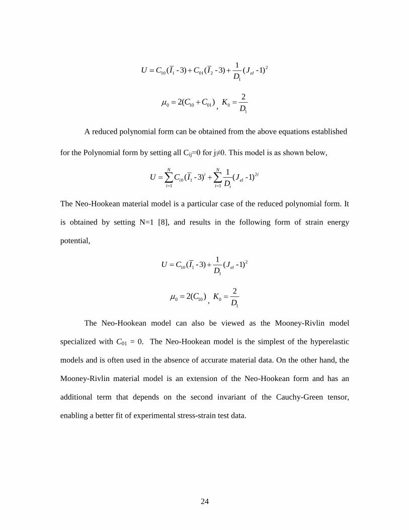
The Neo-Hookean material model is a particular case of the reduced polynomial form. It
is obtained by setting N=1 [8], and results in the following form of strain energy
potential,
2
10 1
1
1( -3) ( -1)elU C I J
D
0 102( )C , 0
1
2K
D
The Neo-Hookean model can also be viewed as the Mooney-Rivlin model
specialized with C01 = 0. The Neo-Hookean model is the simplest of the hyperelastic
models and is often used in the absence of accurate material data. On the other hand, the
Mooney-Rivlin material model is an extension of the Neo-Hookean form and has an
additional term that depends on the second invariant of the Cauchy-Green tensor,
enabling a better fit of experimental stress-strain test data.

25
The material model that is used for the tread of the Tweel™ is a hyperelastic
material model with Neo-Hookean strain energy potential. The shear modulus µ0 and the
bulk modulus K0 are dictated by the coefficients C10 and D1. The density of the material
is 1.1e10-10
daN.sec2/mm
4 (1100 kg/m
3), and the thermal expansion coefficient is
.00017/0C. The coefficient C10 is given as 0.0833, corresponding to an initial shear
modulus of 0.1666 daN/mm2, and coefficient D1 is given as 1.241384, corresponding to
an initial bulk modulus of 1.61 daN/mm2. The specific Hyperelastic material coefficients
defined for the spokes and shear beam will be discussed in detail in Chapter 3.
2.1.2 Orthotropic Elastic material for the reinforcements
The material that is being used for defining the reinforcements that are to be
embedded into the shear beam is an orthotropic elastic material. Orthotropic materials
have three perpendicular mirror planes giving rise to orthotropic symmetry. These
reinforcements are modeled to be relatively inextensible. Since the material is elastic, the
orthotropic relation between strain and stress is of the form,
11 111111 1122 1133
22 222222 2233
33 333333
121212 12
131313 23
232323 31
0 0 0
0 0 0
0 0 0
0 0
0
C C C
C C
C
C
sym C
C
The compliance matrix C, is symmetric and has nine independent compliances.
The constants are directly related to conventional engineering moduli and the Material
Compliance Matrix (C) can be written [13],

26
1312
1 1 1
2321
2 2 2
31 32
3 3 3
12
13
23
--10 0 0
-- 10 0 0
- - 10 0 0
10 0 0 0 0
10 0 0 0 0
10 0 0 0 0
E E E
E E E
E E EC
G
G
G
The Poisson's ratio of an orthotropic material is different in each direction. Due to
the symmetry of the compliance matrix, the Poisson‟s ratios are related by
23 32 31 1312 21
1 2 2 3 3 1
, ,E E E E E E
From above relations we can see that if E1 > E2 then 12 > 21. The larger
Poisson‟s Ratio ( 12 in this case) is called the major Poisson Ratio‟s while the smaller
Poisson‟s Ratio ( 21 in this case) is called minor Poisson‟s Ratio [12]. The inverse of the
Compliance matrix (C) is the Material stiffness matrix (D) relating stress to strain [12],
11 111111 1122 1133
22 222222 2233
33 333333
121212 12
131323 13
232331 23
0 0 0
0 0 0
0 0 0
0 0
0
D D D
D D
D
D
sym D
D
The constants in the material matrix defined in terms of Directional Moduli and
Poisson‟s Ratios are,
27
1111 1 23 32
2222 2 13 31
3333 3 12 21
1122 1 23 32
1133 1 21 31 23 2 12 32 13
1111 1 31 21 32 3 13 12 23
2233 2 32 12 31 3 23 21 13
1212 12
131
(1- )
(1- )
(1- )
(1- )
( ) ( )
( ) ( )
( ) ( )
D E
D E
D E
D E
D E E
D E E
D E E
D G
D
3 13
2323 23
G
D G
where,
12 21 23 32 31 13 21 32 13
1
1- - - - 2
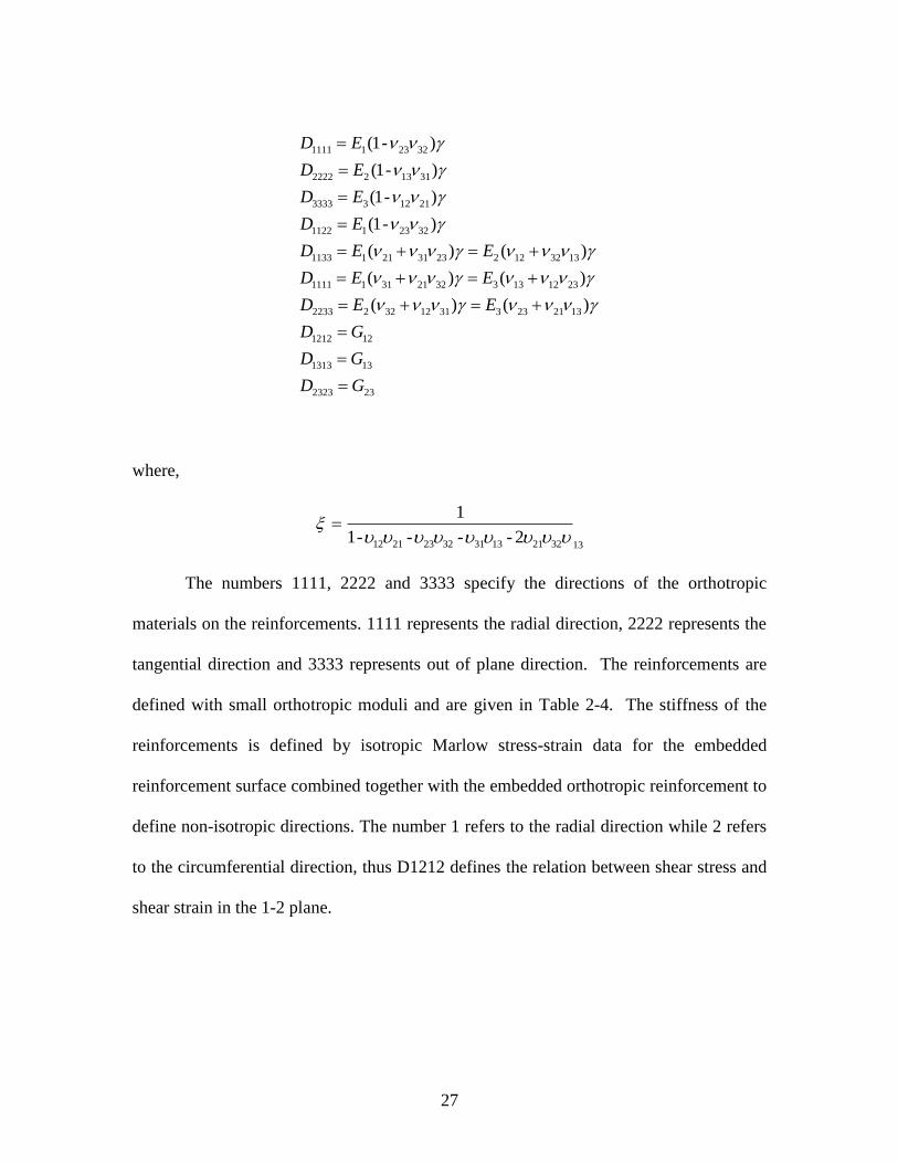
The numbers 1111, 2222 and 3333 specify the directions of the orthotropic
materials on the reinforcements. 1111 represents the radial direction, 2222 represents the
tangential direction and 3333 represents out of plane direction. The reinforcements are
defined with small orthotropic moduli and are given in Table 2-4. The stiffness of the
reinforcements is defined by isotropic Marlow stress-strain data for the embedded
reinforcement surface combined together with the embedded orthotropic reinforcement to
define non-isotropic directions. The number 1 refers to the radial direction while 2 refers
to the circumferential direction, thus D1212 defines the relation between shear stress and
shear strain in the 1-2 plane.

28
Table 2-4: Orthotropic Elastic Moduli coefficients for reinforcements
D1111 D1122 D2222 D1133 D2233 D3333 D1212 D1313 D2323
0.01 0 10 0 0 0.01 10 2 2
The density of the reinforcement material is 1.1E-10 daN.sec2/mm
4 (1100 kg/m
3) and the
thermal expansion coefficient α22 is 1.2E-05/0C.The other components α11 and α33 are 0.
2.2 3D Tweel Mesh and Element Properties
There are different types of elements used for the finite element model which
depend on the intended geometric and analysis type. In ABAQUS, every element is
characterized by the family, degrees of freedom, number of nodes, formulation and
integration. 3D stress elements are used for modeling the shear beam, collapsible spokes
and the reinforcements. The reinforcement surface that houses the reinforcements is
modeled as special surface elements in ABAQUS. The parts that have 3D stress elements
are defined as 8-node linear hexahedral brick element with reduced integration and
hourglass control (C3D8R) [12]. On the other hand, the reinforcement surface has
elements that are 4-node and quadrilateral with reduced integration (SFM3D4R). These
elements are used for Dynamic Explicit analysis only.
When static load deflection analysis is done on the Tweel, a different element
type is used. They are referred to as Hybrid elements. These elements are intended
primarily for use with incompressible and almost incompressible material behavior.
When the material response is incompressible, the solution to a problem cannot be
obtained in terms of the displacement history only, since a purely hydrostatic pressure
29
can be added without changing the displacements. Since hyperelasticity is associated with
incompressibility, hybrid elements are used [12]. The mesh of the shear beam, collapsible
spokes and the reinforcements have 8-node hybrid brick elements (C3D8H). On the other
hand, the reinforcement surface has elements that are 4-node and quadrilateral without
reduced integration (SFM3D4).
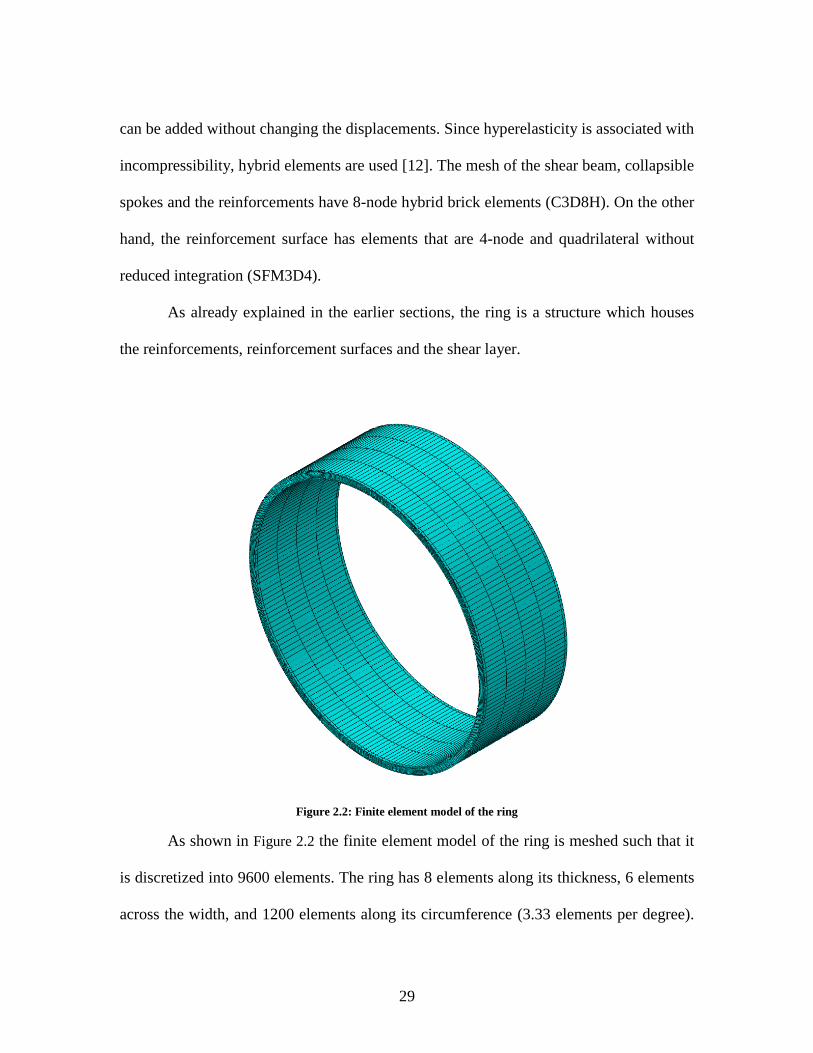
As already explained in the earlier sections, the ring is a structure which houses
the reinforcements, reinforcement surfaces and the shear layer.
Figure 2.2: Finite element model of the ring
As shown in Figure 2.2 the finite element model of the ring is meshed such that it
is discretized into 9600 elements. The ring has 8 elements along its thickness, 6 elements
across the width, and 1200 elements along its circumference (3.33 elements per degree).
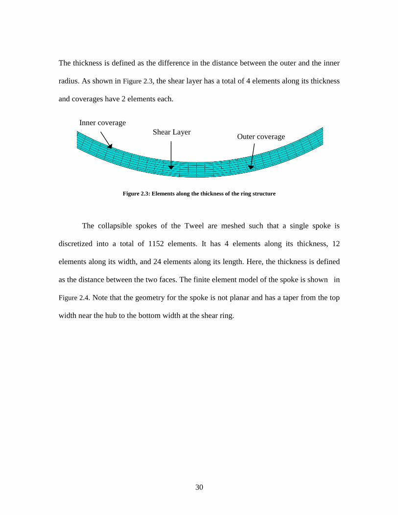
30
The thickness is defined as the difference in the distance between the outer and the inner
radius. As shown in Figure 2.3, the shear layer has a total of 4 elements along its thickness
and coverages have 2 elements each.
Figure 2.3: Elements along the thickness of the ring structure
The collapsible spokes of the Tweel are meshed such that a single spoke is
discretized into a total of 1152 elements. It has 4 elements along its thickness, 12
elements along its width, and 24 elements along its length. Here, the thickness is defined
as the distance between the two faces. The finite element model of the spoke is shown in
Figure 2.4. Note that the geometry for the spoke is not planar and has a taper from the top
width near the hub to the bottom width at the shear ring.
Inner coverage
Shear Layer Outer coverage

31
Figure 2.4: Finite element model of the 3D collapsible spoke. The number of elements across each element are
given in parenthesis.
The tread model is created such that it is an assembly of two half treads. The two
inner surfaces of the half treads are tied together to form an integrated tread model. The
inner surface has 3 elements along its thickness and the outer surface has 1 element along
the thickness. The total elements along the circumference after assembling both the half
treads together are 6000. The integrated tread structure is discretized into 10400
elements.
Spoke Width (12)
Spoke Thickness (4)
Spoke Length (24)

32
Figure 2.5: The inner and outer surfaces of the Finite Element 3D Tread model
Inner surface
(3 elements thru
thickness)
Outer surface
(1 element thru
thicknesss)
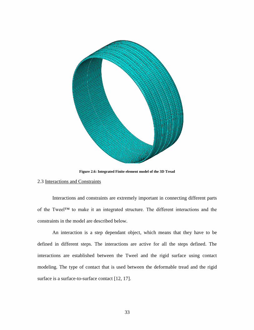
33
Figure 2.6: Integrated Finite element model of the 3D Tread
2.3 Interactions and Constraints
Interactions and constraints are extremely important in connecting different parts
of the Tweel™ to make it an integrated structure. The different interactions and the
constraints in the model are described below.
An interaction is a step dependant object, which means that they have to be
defined in different steps. The interactions are active for all the steps defined. The
interactions are established between the Tweel and the rigid surface using contact
modeling. The type of contact that is used between the deformable tread and the rigid
surface is a surface-to-surface contact [12, 17].

34
For the static load deflection procedure, the contact model is defined in
ABAQUS/Standard. The sliding formulation between the rigid surface and the
deformable tread is finite sliding. The discretization method that defines the contact
model is surface-to-surface. A tangential interaction property is defined to be frictionless
for the interaction between the two surfaces. In this analysis, the Tweel is not subjected to
rolling and hence, to establish contact, it is not mandatory to select the entire tread
surface.
Figure 2.7: Surface-to-surface interaction established between the tread surface and the rigid ground
For the dynamic rolling analysis, the contact model is defined in ABAQUS /
Explicit. The mechanical constraint formulation between the rigid surface and the
deformable tread is defined by penalty contact method. The sliding formulation is finite
sliding. The tangential interaction property is defined as a penalty contact method with a
friction coefficient value of 1. In both static general and dynamic explicit, a normal
Interacting surface

35
interaction property is defined such that the pressure over closure is “Hard” contact. Also,
the contacting surfaces are allowed to separate during the analysis.
In a dynamic explicit analysis, the surfaces have to be continuous for an
interaction to be established. Since the tread is divided into 6 grooves, the outer tread
surface is no longer continuous. Hence 6 different interactions have been created. Also,
since the Tweel is subjected to rolling in this analysis, the entire tread surface is selected.
Figure 2.8: Surface-to-surface contact established between the tread surfaces and rigid ground.
The constraints used in the model to form an integrated Tweel are Tie, Coupling
and Embedded Regions. They are described below.
Interacting surface

36
2.3.1 Constraint - Embedded Region
An embedded region constraint allows one to embed a region of the model within
another region of the model or within the whole model. Embedded region constraint is
based on the embedded element technique. These elements are assembled within the
“host” structure whose response will be used to constrain the translational degrees of
freedom of the nodes of the embedded elements [12]. This constraint is used to embed the
reinforcements and reinforcement surfaces into the ring, which is the host structure.
These in-extensible membranes are assembled such that the shear layer lies between the
two reinforcements. The reinforcement surfaces are assembled above the reinforcements.
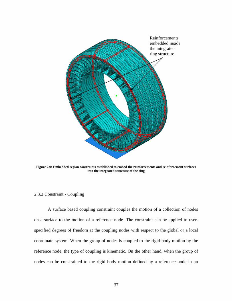
37
Figure 2.9: Embedded region constraints established to embed the reinforcements and reinforcement surfaces
into the integrated structure of the ring
2.3.2 Constraint - Coupling
A surface based coupling constraint couples the motion of a collection of nodes
on a surface to the motion of a reference node. The constraint can be applied to user-
specified degrees of freedom at the coupling nodes with respect to the global or a local
coordinate system. When the group of nodes is coupled to the rigid body motion by the
reference node, the type of coupling is kinematic. On the other hand, when the group of
nodes can be constrained to the rigid body motion defined by a reference node in an
Reinforcements
embedded inside
the integrated
ring structure
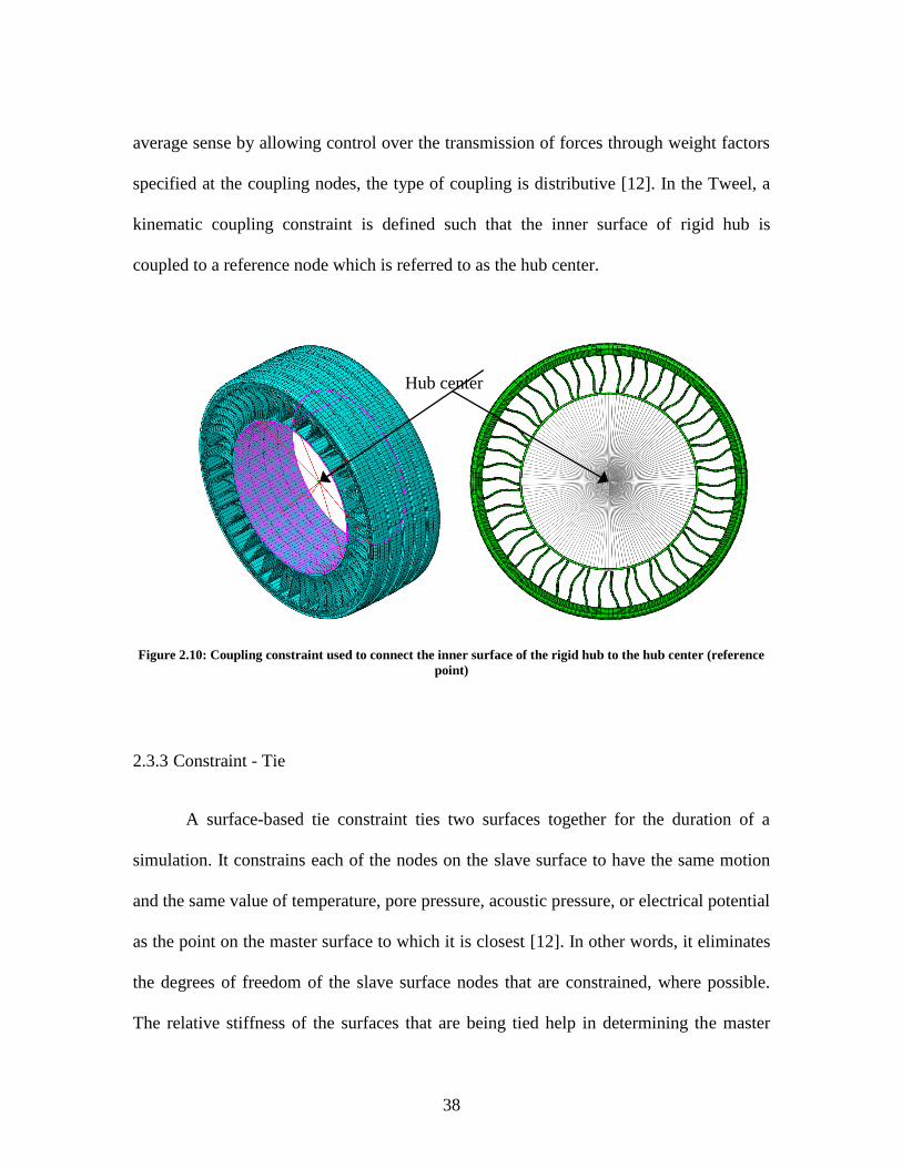
38
average sense by allowing control over the transmission of forces through weight factors
specified at the coupling nodes, the type of coupling is distributive [12]. In the Tweel, a
kinematic coupling constraint is defined such that the inner surface of rigid hub is
coupled to a reference node which is referred to as the hub center.
Figure 2.10: Coupling constraint used to connect the inner surface of the rigid hub to the hub center (reference
point)
2.3.3 Constraint - Tie
A surface-based tie constraint ties two surfaces together for the duration of a
simulation. It constrains each of the nodes on the slave surface to have the same motion
and the same value of temperature, pore pressure, acoustic pressure, or electrical potential
as the point on the master surface to which it is closest [12]. In other words, it eliminates
the degrees of freedom of the slave surface nodes that are constrained, where possible.
The relative stiffness of the surfaces that are being tied help in determining the master
Hub center
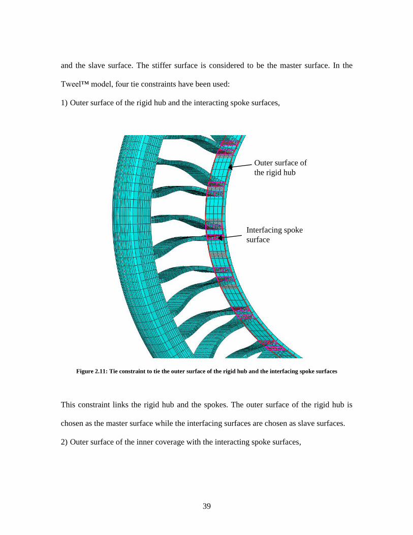
39
and the slave surface. The stiffer surface is considered to be the master surface. In the
Tweel™ model, four tie constraints have been used:
1) Outer surface of the rigid hub and the interacting spoke surfaces,
Figure 2.11: Tie constraint to tie the outer surface of the rigid hub and the interfacing spoke surfaces
This constraint links the rigid hub and the spokes. The outer surface of the rigid hub is
chosen as the master surface while the interfacing surfaces are chosen as slave surfaces.
2) Outer surface of the inner coverage with the interacting spoke surfaces,
Outer surface of
the rigid hub
Interfacing spoke
surface
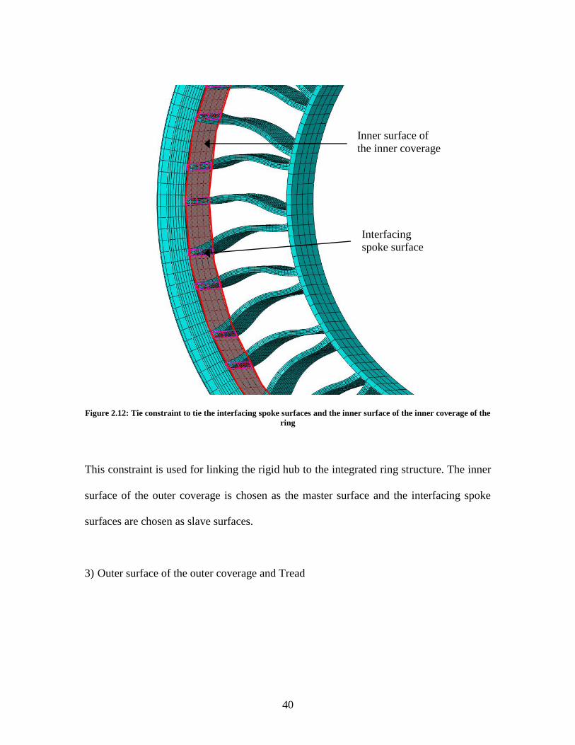
40
Figure 2.12: Tie constraint to tie the interfacing spoke surfaces and the inner surface of the inner coverage of the
ring
This constraint is used for linking the rigid hub to the integrated ring structure. The inner
surface of the outer coverage is chosen as the master surface and the interfacing spoke
surfaces are chosen as slave surfaces.
3) Outer surface of the outer coverage and Tread
Inner surface of
the inner coverage
Interfacing
spoke surface

41
Figure 2.13: Tie constraint to tie the outer surface of the outer coverage and the tread
This constraint links the integrated ring structure and the deformable tread. The outer
surface of the outer coverage is selected as the master surface and the inner surface of the
tread is selected as the slave surface.
4) Both half tread models
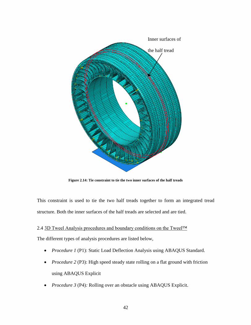
42
Figure 2.14: Tie constraint to tie the two inner surfaces of the half treads
This constraint is used to tie the two half treads together to form an integrated tread
structure. Both the inner surfaces of the half treads are selected and are tied.
2.4 3D Tweel Analysis procedures and boundary conditions on the Tweel™
The different types of analysis procedures are listed below,
Procedure 1 (P1): Static Load Deflection Analysis using ABAQUS Standard.
Procedure 2 (P3): High speed steady state rolling on a flat ground with friction
using ABAQUS Explicit
Procedure 3 (P4): Rolling over an obstacle using ABAQUS Explicit.
Inner surfaces of
the half tread

43
2.4.1 Static Load Deflection
This computational procedure for the TWEEL model is divided into two steps.
1. Predefined field: Temperature of the model is set to 125 0C
2. Step 0: Initial Condition: Temperature is 125 0C.
3. Step 1: Cooling: A 50 0C temperature change is brought about over a time period
of 0.1 seconds.
4. Step 2: Loading: Temperature is maintained at 75 0C and a load of 366.5 daN (824
lb) is applied at the hub center over a time period of 0.1 seconds. This weight
corresponds to the quarter weight of the vehicle.
This procedure is executed in ABAQUS Standard and is used to find out the
corresponding displacement of the model in the vertical direction when a vertical force is
applied at the hub center. This procedure is described below in further detail.
In Step 1, the Tweel is at an initial temperature of 125 0C and the model is
completely stationary. The temperature is reduced by 500C to model the molding process
in manufacturing so that the Tweel develops pre-stress due to thermal strains. The ring
contracts when the Tweel is cooled from 125 0C to 75
0C. As a result, the Tweel tends to
lose contact with the ground. An adjustment has been made to avoid loss of contact
during this step. The ground is tied to the tread of the Tweel and is allowed to move
freely in the vertical direction during cooling. When step 2 commences, the temperature
is maintained at 75 0C and a vertical load of 366.5 daN is applied at the hub center. The
ground is completely constrained when the load is being applied. Due to the application
of load, the Tweel is compressed against the ground and hence the displacement of the

44
hub center in the vertical direction is obtained. This is referred to as the “deflection” of
the Tweel upon the action of a “load”.
Figure 2.15: Boundary conditions imposed on the Tweel during static load deflection procedure
2.4.2 High speed steady state rolling on a flat ground with friction
This procedure is divided into three steps.
1. Predefined field: Temperature of the model is set to 125 0C
2. Step 0: Temperature is 1250C. The ground and the hub center are fixed.
3. Step 1: Loading, Acceleration and Cooling: Temperature is reduced to 750C. A
load of 366.5 daN is applied. Hub center is free to move in the vertical direction
Hub center is free
to move downwards
due to the
application of load
Uniform temperature
change from 125 to 75
throughout the
model in step 1
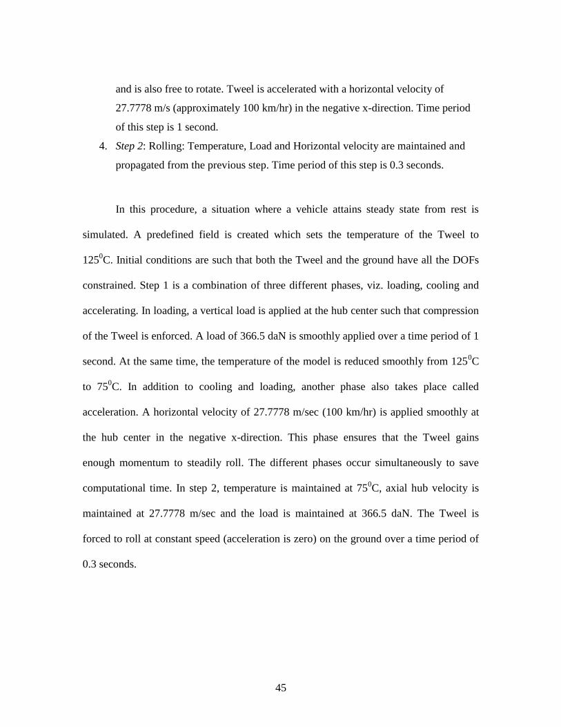
45
and is also free to rotate. Tweel is accelerated with a horizontal velocity of
27.7778 m/s (approximately 100 km/hr) in the negative x-direction. Time period
of this step is 1 second.
4. Step 2: Rolling: Temperature, Load and Horizontal velocity are maintained and
propagated from the previous step. Time period of this step is 0.3 seconds.
In this procedure, a situation where a vehicle attains steady state from rest is
simulated. A predefined field is created which sets the temperature of the Tweel to
1250C. Initial conditions are such that both the Tweel and the ground have all the DOFs
constrained. Step 1 is a combination of three different phases, viz. loading, cooling and
accelerating. In loading, a vertical load is applied at the hub center such that compression
of the Tweel is enforced. A load of 366.5 daN is smoothly applied over a time period of 1
second. At the same time, the temperature of the model is reduced smoothly from 1250C
to 750C. In addition to cooling and loading, another phase also takes place called
acceleration. A horizontal velocity of 27.7778 m/sec (100 km/hr) is applied smoothly at
the hub center in the negative x-direction. This phase ensures that the Tweel gains
enough momentum to steadily roll. The different phases occur simultaneously to save
computational time. In step 2, temperature is maintained at 750C, axial hub velocity is
maintained at 27.7778 m/sec and the load is maintained at 366.5 daN. The Tweel is
forced to roll at constant speed (acceleration is zero) on the ground over a time period of
0.3 seconds.

46
2.4.3 Rolling over an obstacle
This procedure is divided into three steps.
Predefined field: Temperature of the model is set to 125 0C
1. Step 0: Temperature is 1250C. The ground and the hub center are fixed.
2. Step 1: Loading, Acceleration and Cooling: Temperature is reduced to 750C. A
load of 366.5 daN is applied. Hub center is free to move in the vertical direction
and is also free to rotate. Tweel is accelerated with a horizontal velocity of 3m/s.
Time period of this step is 1 second.
3. Step 2: Intermediate: Temperature, Load and Horizontal velocity are maintained
are maintained a constant from the previous step. Time period of this step is 0.1
seconds.
4. Step 3: Free Rolling: Temperature is maintained at the same value from the
previous step. The horizontal velocity is no longer maintained at 3 m/s (10.8
km/hr). No boundary condition is enforced at the hub center
In this procedure, a situation where a vehicle attains steady state from rest is
simulated. A predefined field is created which sets the temperature of the Tweel to
1250C. Initial conditions are such that both the Tweel and the ground have all the DOFs
constrained. Step 1 is a combination of three different analyses, viz. loading, cooling and
accelerating. In loading, a vertical load is applied at the hub center such that compression
of the Tweel is enforced. A load of 366.5 daN (824 lb) is smoothly applied over a time
period of 1 second. At the same time, the temperature of the model is reduced smoothly
from 1250C to 75
0C. In addition to cooling and loading, another phase also takes place
called acceleration. A horizontal velocity of 3 m/second is applied smoothly at the hub
center. This phase ensures that the Tweel gains enough momentum to steadily roll. The

47
different phases occur simultaneously to save computational time. In step 2, temperature
is maintained at 750C, axial hub velocity is maintained at 3m/sec and the load is
maintained at 366.5 daN. The Tweel is forced to roll at constant speed (acceleration is
zero) on the ground over a time period of 0.1 seconds. In Step 3, all the other conditions
remain the same from the previous step except for the axial velocity which is made
inactive. This can be related to a situation where the driver of the vehicle takes his/her
foot off the accelerator. Once the acceleration is not provided, the Tweel travels due to
the momentum generated in the previous step.
Figure 2.16: Boundary conditions imposed on the Tweel during loading, accelerating and cooling (step 1) in
procedures 2 and 3
Uniform temperature
change from 125 0C
to 75 0C throughout
the model
Axial hub velocity
(P3) – 27.778 m/s
Axial hub velocity
(P4) – 3 m/s 366.5 dN vertical load
applied at hub center
Free to rotate

48
CHAPTER THREE – EFFECTS OF CHANGING MATERIAL MODELS ON STRESS-
STRAIN CURVES
There are many factors that may affect the noise level and/or vibrations of the
TWEEL. They may be classified as Geometric, Material and other factors. Geometric
factors include spoke curvature; spoke thickness, ring dimensions and number of shear
ring reinforcements. Material factors may include the stiffness characteristics, mass,
damping, and nonlinear material models used for the spoke, ring, reinforcements and tire
tread. In this chapter, a detailed explanation of the different material models used for the
spokes, ring and reinforcements are given. Also, the stress-strain curves for the different
material models are analyzed and compared.
3.1 Material models
The reference Tweel model uses a hyperelastic Marlow material model for the
ring and the spokes. The properties for this material model have been obtained from the
uni-axial test data for polyurethane (PU). In addition, two material models have been
selected to study the effects of changing material stiffness. They are,
1) Mooney Rivlin
This material model has been derived from the general polynomial strain energy
potential form. The polynomial strain energy potential is given below,
2
1 2
1 1
1( -3) ( -3) ( -1)
N Ni j i
ij el
i j i i
U C I I JD
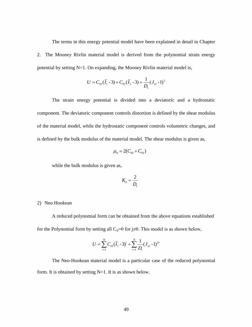
49
The terms in this energy potential model have been explained in detail in Chapter
2. The Mooney Rivlin material model is derived from the polynomial strain energy
potential by setting N=1. On expanding, the Mooney Rivlin material model is,
2
10 1 01 2
1
1( -3) ( -3) ( -1)elU C I C I J
D
The strain energy potential is divided into a deviatoric and a hydrostatic
component. The deviatoric component controls distortion is defined by the shear modulus
of the material model, while the hydrostatic component controls volumetric changes, and
is defined by the bulk modulus of the material model. The shear modulus is given as,
0 10 012( )C C
while the bulk modulus is given as,
0
1
2K
D
2) Neo Hookean
A reduced polynomial form can be obtained from the above equations established
for the Polynomial form by setting all Cij=0 for j≠0. This model is as shown below,
2
0 1
1 1
1( -3) ( -1)
N Ni i
i el
i i i
U C I JD
The Neo-Hookean material model is a particular case of the reduced polynomial
form. It is obtained by setting N=1. It is as shown below.
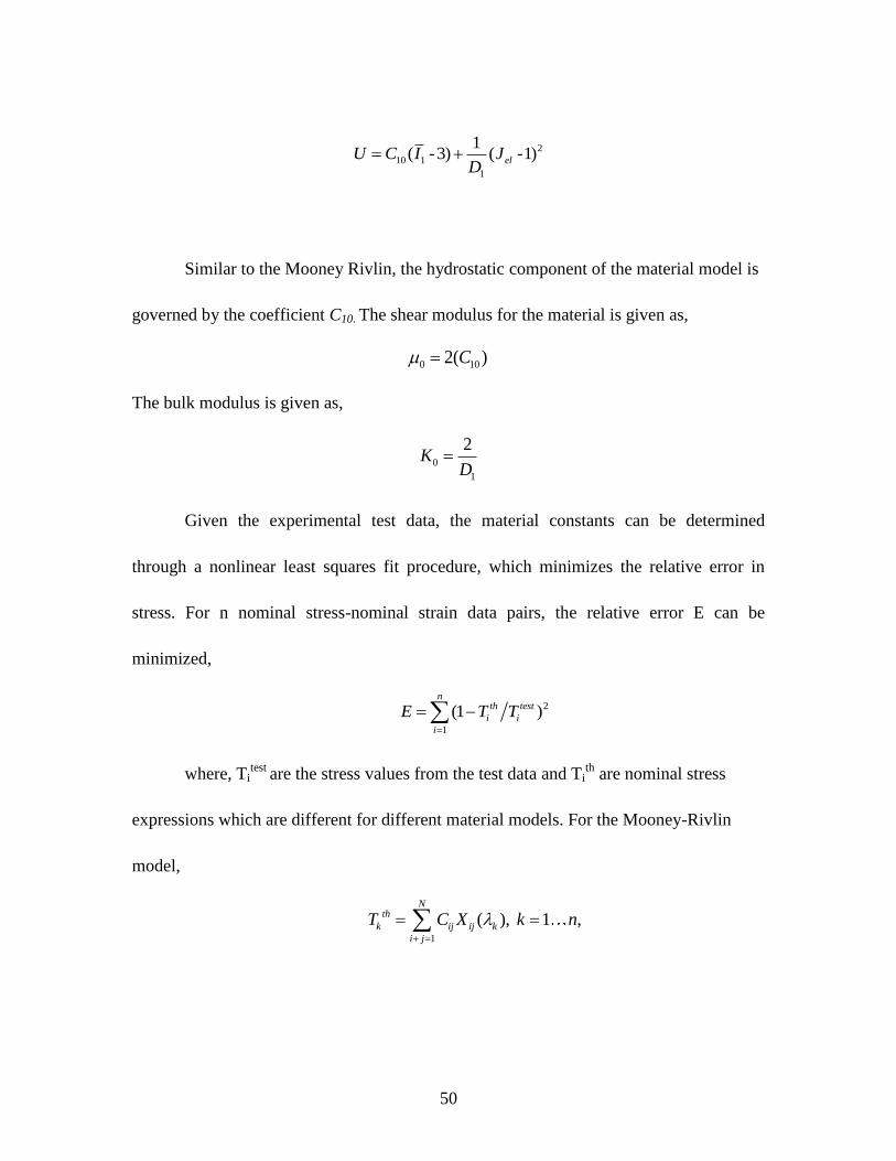
50
2
10 1
1
1( -3) ( -1)elU C I J
D
Similar to the Mooney Rivlin, the hydrostatic component of the material model is
governed by the coefficient C10. The shear modulus for the material is given as,
0 102( )C
The bulk modulus is given as,
0
1
2K
D
Given the experimental test data, the material constants can be determined
through a nonlinear least squares fit procedure, which minimizes the relative error in
stress. For n nominal stress-nominal strain data pairs, the relative error E can be
minimized,
2
1
(1 )n
th test
i i
i
E T T
where, Titest
are the stress values from the test data and Tith
are nominal stress
expressions which are different for different material models. For the Mooney-Rivlin
model,
1
( ), 1 ,N
th
k ij ij k
i j
T C X k n
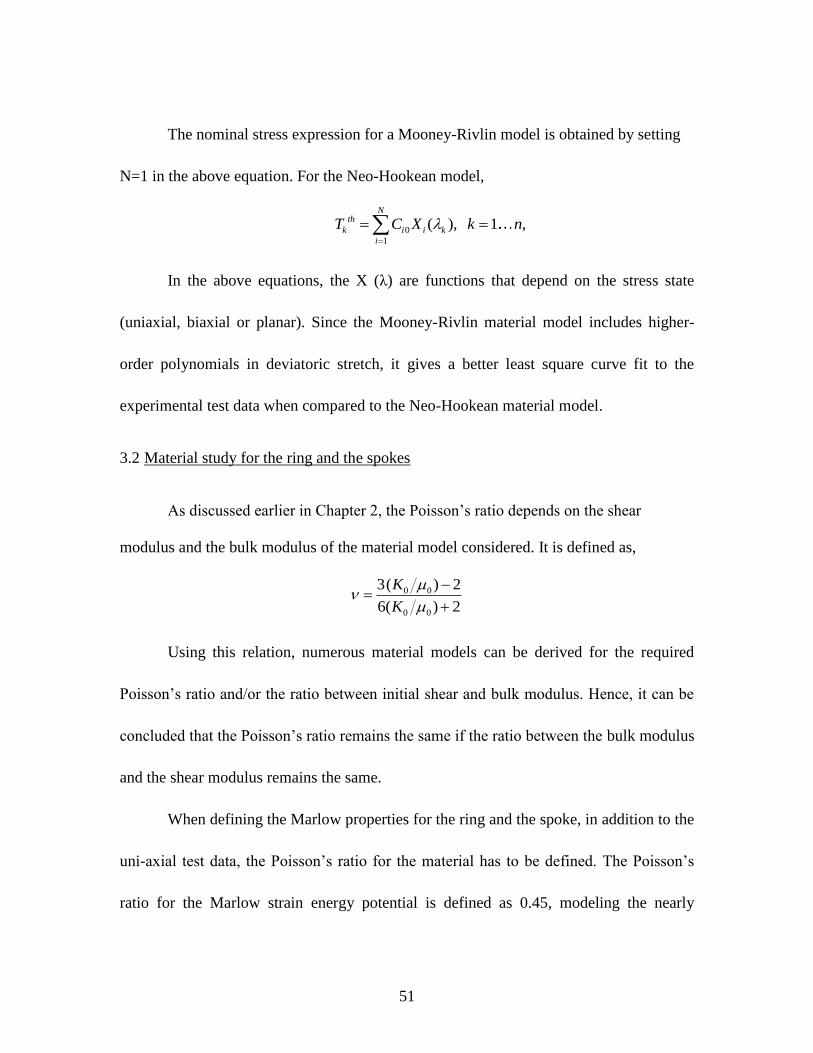
51
The nominal stress expression for a Mooney-Rivlin model is obtained by setting
N=1 in the above equation. For the Neo-Hookean model,
0
1
( ), 1 ,N
th
k i i k
i
T C X k n
In the above equations, the X (λ) are functions that depend on the stress state
(uniaxial, biaxial or planar). Since the Mooney-Rivlin material model includes higher-
order polynomials in deviatoric stretch, it gives a better least square curve fit to the
experimental test data when compared to the Neo-Hookean material model.
3.2 Material study for the ring and the spokes
As discussed earlier in Chapter 2, the Poisson‟s ratio depends on the shear
modulus and the bulk modulus of the material model considered. It is defined as,
0 0
0 0
3( ) 2
6( ) 2
K
K
Using this relation, numerous material models can be derived for the required
Poisson‟s ratio and/or the ratio between initial shear and bulk modulus. Hence, it can be
concluded that the Poisson‟s ratio remains the same if the ratio between the bulk modulus
and the shear modulus remains the same.
When defining the Marlow properties for the ring and the spoke, in addition to the
uni-axial test data, the Poisson‟s ratio for the material has to be defined. The Poisson‟s
ratio for the Marlow strain energy potential is defined as 0.45, modeling the nearly

52
incompressible nature of polyurethane (PU). To study the effect of changing material
models for the ring and the spokes of the Tweel, different material models are generated
with the same Poisson‟s ratio of 0.45. From the above equation, the ratio of the bulk
modulus and the shear modulus is defined as,
0
0
2(1 )
3(1 2 )
K
From this equation, the ratio of the initial bulk modulus to the initial shear
modulus is 29/3. In this material study, Mooney Rivlin and Neo Hookean material
models are fit to the Marlow strain energy potential. The Mooney Rivlin and Neo
Hookean models allow us to change the material behavior by a defined amount by
changing the coefficients in the model. Three levels are defined for every material
thereby making it a total of 6 materials in addition to the Marlow strain energy potential.
The first level is when the shear modulus of the material remains unchanged. The second
level is when the shear modulus of the material is reduced by 25%. Finally the third level
is when the shear modulus is increased by 25%. For each of these models, the bulk
modulus is adjusted in order to keep the same Poisson‟s ratio as the reference Marlow
model.
For the Mooney Rivlin material model, the ratio of the initial bulk modulus and
the initial shear modulus is defined as,
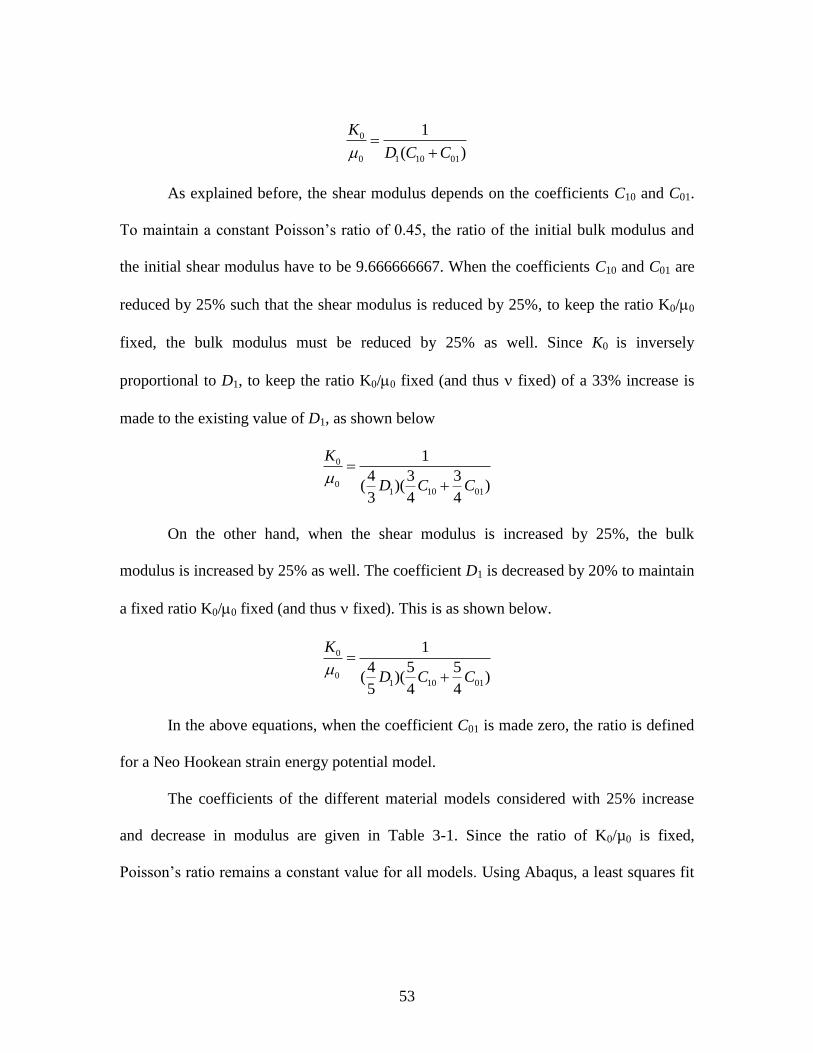
53
0
0 1 10 01
1
( )
K
D C C
As explained before, the shear modulus depends on the coefficients C10 and C01.
To maintain a constant Poisson‟s ratio of 0.45, the ratio of the initial bulk modulus and
the initial shear modulus have to be 9.666666667. When the coefficients C10 and C01 are
reduced by 25% such that the shear modulus is reduced by 25%, to keep the ratio K0/0
fixed, the bulk modulus must be reduced by 25% as well. Since K0 is inversely
proportional to D1, to keep the ratio K0/0 fixed (and thus fixed) of a 33% increase is
made to the existing value of D1, as shown below
0
01 10 01
1
4 3 3( )( )3 4 4
K
D C C
On the other hand, when the shear modulus is increased by 25%, the bulk
modulus is increased by 25% as well. The coefficient D1 is decreased by 20% to maintain
a fixed ratio K0/0 fixed (and thus fixed). This is as shown below.
0
01 10 01
1
4 5 5( )( )5 4 4
K
D C C
In the above equations, when the coefficient C01 is made zero, the ratio is defined
for a Neo Hookean strain energy potential model.
The coefficients of the different material models considered with 25% increase
and decrease in modulus are given in Table 3-1. Since the ratio of K0/µ0 is fixed,
Poisson‟s ratio remains a constant value for all models. Using Abaqus, a least squares fit

54
of the Marlow data is used to determine the unchanged coefficients (denoted as 0%) in
the Mooney-Rivlin and Neo-Hookean models.
Table 3-1: Hyperelastic Material Coefficients used in the material study for the ring and spokes. Units for
moduli are dN/mm2. Fixed Poisson’s ratio ν = 0.45, K0/µ0=9.6667
Material D1 C10 C01
Shear
Modulus
µ0
Bulk
Modulus
K0
Mooney-
Rivlin
+25% .099552403 -.968195876 2.00732976 2.078267768 20.08992189
0% .124440504 -.774556701 1.60586381 1.662614218 16.07193748
-25% .165920257 -.580917525 1.20439786 1.24696067 12.05398326
Neo-
Hookean
+25% .168449137 .614121730 0 1.22824346 11.87302016
0% .210561422 .491297384 0 .982594768 9.498416096
-25% .280748562 .368473038 0 .736946076 7.123812089
3.3 Comparison of nominal stress – nominal strain curves
The nominal stress – nominal strain curves for the different Hyperelastic material
models are obtained by evaluating the coefficients using ABAQUS. The following set of
nominal stress – nominal strain curves are provided for all the material models. The range
of the nominal values of strain is from -0.2 to +0.2. The strains are plotted on the X-axis
and their corresponding nominal stress values are plotted on the Y-axis.
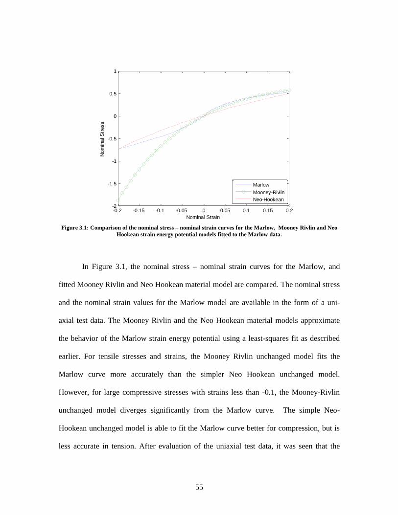
55
Figure 3.1: Comparison of the nominal stress – nominal strain curves for the Marlow, Mooney Rivlin and Neo
Hookean strain energy potential models fitted to the Marlow data.
In Figure 3.1, the nominal stress – nominal strain curves for the Marlow, and
fitted Mooney Rivlin and Neo Hookean material model are compared. The nominal stress
and the nominal strain values for the Marlow model are available in the form of a uni-
axial test data. The Mooney Rivlin and the Neo Hookean material models approximate
the behavior of the Marlow strain energy potential using a least-squares fit as described
earlier. For tensile stresses and strains, the Mooney Rivlin unchanged model fits the
Marlow curve more accurately than the simpler Neo Hookean unchanged model.
However, for large compressive stresses with strains less than -0.1, the Mooney-Rivlin
unchanged model diverges significantly from the Marlow curve. The simple Neo-
Hookean unchanged model is able to fit the Marlow curve better for compression, but is
less accurate in tension. After evaluation of the uniaxial test data, it was seen that the
-0.2 -0.15 -0.1 -0.05 0 0.05 0.1 0.15 0.2-2
-1.5
-1
-0.5
0
0.5
1
Nominal Strain
Nom
inal S
tress
Marlow
Mooney-Rivlin
Neo-Hookean
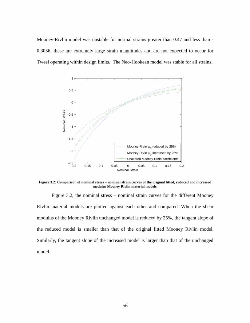
56
Mooney-Rivlin model was unstable for normal strains greater than 0.47 and less than -
0.3056; these are extremely large strain magnitudes and are not expected to occur for
Tweel operating within design limits. The Neo-Hookean model was stable for all strains.
Figure 3.2: Comparison of nominal stress – nominal strain curves of the original fitted, reduced and increased
modulus Mooney Rivlin material models.
Figure 3.2, the nominal stress – nominal strain curves for the different Mooney
Rivlin material models are plotted against each other and compared. When the shear
modulus of the Mooney Rivlin unchanged model is reduced by 25%, the tangent slope of
the reduced model is smaller than that of the original fitted Mooney Rivlin model.
Similarly, the tangent slope of the increased model is larger than that of the unchanged
model.
-0.2 -0.15 -0.1 -0.05 0 0.05 0.1 0.15 0.2-2.5
-2
-1.5
-1
-0.5
0
0.5
1
Nominal Strain
Nom
inal S
tress
Mooney-Rivlin 0 reduced by 25%
Mooney-Rivlin 0 increased by 25%
Unaltered Mooney-Rivlin coefficients

57
Figure 3.3: Comparison of nominal stress – nominal strain curves of the original fitted, reduced and increased
modulus Mooney Rivlin material models.
In Figure 4.4 the nominal stress – nominal strain curves for the different Neo
Hookean material models are plotted against each other and compared. When the shear
modulus of the Neo Hookean unchanged model is reduced by 25%, the tangent slope of
the reduced model is smaller than that of the unchanged model. Similarly, the tangent
slope of the increased model is larger than that of the unchanged model.
As already explained, the shear modulus can be related directly to the stiffness of
the material model. Based on the results, it can be concluded that the higher the shear
modulus, the more the stiffness of the material model and vice versa.
-0.2 -0.15 -0.1 -0.05 0 0.05 0.1 0.15 0.2-1
-0.8
-0.6
-0.4
-0.2
0
0.2
0.4
0.6
0.8
Nominal Strain
Nom
inal S
tress
Neo-Hookean 0 reduced by 25%
Neo-Hookean 0 increased by 25%
Unaltered Neo-Hookean coefficients
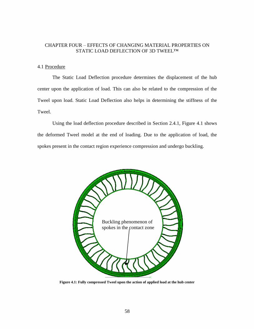
58
CHAPTER FOUR – EFFECTS OF CHANGING MATERIAL PROPERTIES ON
STATIC LOAD DEFLECTION OF 3D TWEEL™
4.1 Procedure
The Static Load Deflection procedure determines the displacement of the hub
center upon the application of load. This can also be related to the compression of the
Tweel upon load. Static Load Deflection also helps in determining the stiffness of the
Tweel.
Using the load deflection procedure described in Section 2.4.1, Figure 4.1 shows
the deformed Tweel model at the end of loading. Due to the application of load, the
spokes present in the contact region experience compression and undergo buckling.
Figure 4.1: Fully compressed Tweel upon the action of applied load at the hub center
Buckling phenomenon of
spokes in the contact zone

59
4.2 Comparison of Static Load Deflection curves
In the following static load-deflection curves are generated for the Tweel models
with different material properties. In the first section, the material properties and of the
different Hyperelastic models for the polyurethane in the ring are changed while keeping
the Marlow model for the polyurethane in the spokes unchanged. In the second study, the
material properties of the polyurethane spoke are changed while keeping the original
Marlow model for polyurethane in the ring unchanged. The load-deflection curves were
obtained by combining the vertical reaction force exerted on the wheel with respect to
time and the corresponding vertical displacement with respect to time. Ask discussed
earlier, for each model studied, the ratio of initial bulk modulus to shear modulus is kept
constant. The values on the Y-axis correspond to the reaction force in deca Newton (dN)
on the TWEEL and the corresponding vertical displacement values in millimeter (mm)
are plotted on the X-axis.
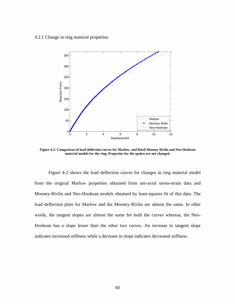
60
4.2.1 Change in ring material properties
Figure 4.2: Comparison of load deflection curves for Marlow, and fitted Mooney Rivlin and Neo Hookean
material models for the ring. Properties for the spokes are not changed.
Figure 4-2 shows the load deflection curves for changes in ring material model
from the original Marlow properties obtained from uni-axial stress-strain data and
Mooney-Rivlin and Neo-Hookean models obtained by least-squares fit of this data. The
load deflection plots for Marlow and the Mooney-Rivlin are almost the same. In other
words, the tangent slopes are almost the same for both the curves whereas, the Neo-
Hookean has a slope lesser than the other two curves. An increase in tangent slope
indicates increased stiffness while a decrease in slope indicates decreased stiffness.
0 2 4 6 8 10 120
50
100
150
200
250
300
350
Displacement
Reaction F
orc
e
Marlow
Mooney-Rivlin
Neo-Hookean

61
Figure 4.3: Comparison of load deflection curves for different Mooney Rivlin models for the ring. Properties for
spoke are not changed.
Figure 4.3and Figure 4.4 show the load deflection curves for cases when the
initial shear modulus for the Mooney-Rivlin and Neo-Hookean models is changed by
plus/minus 25%. It is seen that as the shear modulus is increased, the tangent slope
increases as well. Since the vertical stiffness can be correlated with the tangent slope, it is
concluded that the vertical stiffness is directly proportional to the shear modulus.
0 2 4 6 8 10 120
50
100
150
200
250
300
350
Displacement
Reaction F
orc
e
Mooney-Rivlin 0 reduced by 25%
Mooney-Rivlin 0 increased by 25%
Mooney-Rivlin 0 unchanged
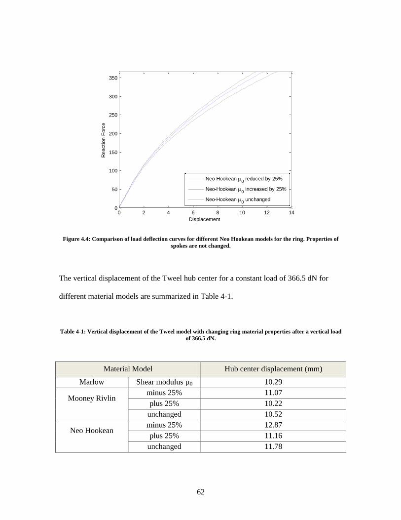
62
Figure 4.4: Comparison of load deflection curves for different Neo Hookean models for the ring. Properties of
spokes are not changed.
The vertical displacement of the Tweel hub center for a constant load of 366.5 dN for
different material models are summarized in Table 4-1.
Table 4-1: Vertical displacement of the Tweel model with changing ring material properties after a vertical load
of 366.5 dN.
Material Model Hub center displacement (mm)
Marlow Shear modulus µ0 10.29
Mooney Rivlin
minus 25% 11.07
plus 25% 10.22
unchanged 10.52
Neo Hookean
minus 25% 12.87
plus 25% 11.16
unchanged 11.78
0 2 4 6 8 10 12 140
50
100
150
200
250
300
350
Displacement
Reaction F
orc
e
Neo-Hookean 0 reduced by 25%
Neo-Hookean 0 increased by 25%
Neo-Hookean 0 unchanged
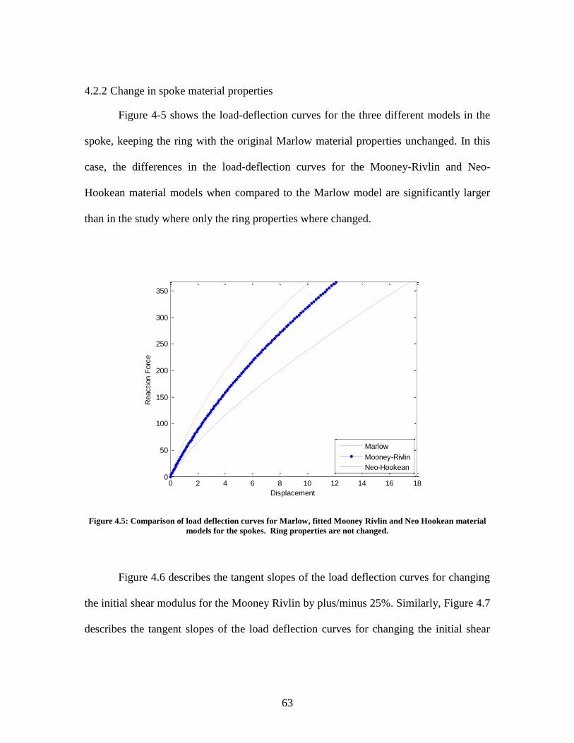
63
4.2.2 Change in spoke material properties
Figure 4-5 shows the load-deflection curves for the three different models in the
spoke, keeping the ring with the original Marlow material properties unchanged. In this
case, the differences in the load-deflection curves for the Mooney-Rivlin and Neo-
Hookean material models when compared to the Marlow model are significantly larger
than in the study where only the ring properties where changed.
Figure 4.5: Comparison of load deflection curves for Marlow, fitted Mooney Rivlin and Neo Hookean material
models for the spokes. Ring properties are not changed.
Figure 4.6 describes the tangent slopes of the load deflection curves for changing
the initial shear modulus for the Mooney Rivlin by plus/minus 25%. Similarly, Figure 4.7
describes the tangent slopes of the load deflection curves for changing the initial shear
0 2 4 6 8 10 12 14 16 180
50
100
150
200
250
300
350
Displacement
Reaction F
orc
e
Marlow
Mooney-Rivlin
Neo-Hookean
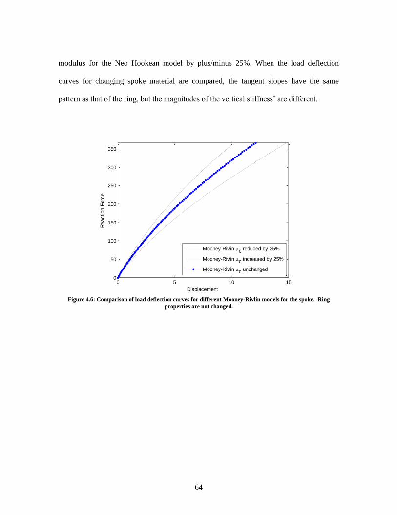
64
modulus for the Neo Hookean model by plus/minus 25%. When the load deflection
curves for changing spoke material are compared, the tangent slopes have the same
pattern as that of the ring, but the magnitudes of the vertical stiffness‟ are different.
Figure 4.6: Comparison of load deflection curves for different Mooney-Rivlin models for the spoke. Ring
properties are not changed.
0 5 10 150
50
100
150
200
250
300
350
Displacement
Reaction F
orc
e
Mooney-Rivlin 0 reduced by 25%
Mooney-Rivlin 0 increased by 25%
Mooney-Rivlin 0 unchanged

65
Figure 4.7: Comparison of load deflection curves for different Neo Hookean models for the spoke. Ring
properties are not changed.
The deflections for a constant load of 366.5 dN for different material models are
summarized in Table 4-2. From the values provided in Table 4-1 and Table 4-2, it is seen
that the Tweel deflects more when its stiffness is less and vice versa.
Table 4-2: Vertical displacement of the Tweel model with changing spoke material properties after a vertical
load of 366.5 dN.
Material Model Deflection (mm)
Marlow Shear modulus µ0 10.29
Mooney Rivlin
minus 25% 14.88
plus 25% 10.25
unchanged 12.11
Neo Hookean
minus 25% 20.84
plus 25% 15.12
unchanged 17.5
0 5 10 15 20 250
50
100
150
200
250
300
350
Displacement
Reaction F
orc
e
Neo-Hookean 0 reduced by 25%
Neo-Hookean 0 increased by 25%
Neo-Hookean 0 unchanged

66
CHAPTER FIVE – EFFECTS OF CHANGING MATERIAL PROPERTIES ON
STEADY STATE ROLLING ON A FLAT GROUND
From [3, 4, 5, 6, 7], it has been hypothesized that the prime sources of noise and
vibration produced by the Tweel include spoke vibration, ring vibration and ground
contact interaction. When the spokes come into the contact zone, they buckle due to the
application of load and snap back into tension on exiting the contact zone. This behavior
of the spokes creates vibration, which may lead to unwanted sound radiation and noise.
Since the spokes are connected to the ring, this causes the ring to vibrate, and visa versa.
Another source of noise and vibration is due to the shearing of the shear beam and the
bending of the integrated ring structure when in the contact zone. Due to application of
load, the contact patch created by the Tweel with the ground becomes flat and causing the
entire ring to vibrate. As a result, the tread starts to vibrate along with the ring and causes
fluctuations in the contact forces. This also can be a possible source of noise.
In [3, 4, 5, 6, 7], spoke vibration, ring vibration and ground reaction forces were
investigated to study the vibrations produced by the Tweel. All these previous studied
used a planar model for the Tweel. In [3,4], the time-signal for changes in spoke length
from the 2D planar model are transferred as boundary conditions for a detailed 3D single
spoke model. As discussed in the thesis objectives in Chapter 1, a goal of this work is to
study spoke and ground force vibration using a complete 3D Tweel model. In addition,
in order to remove any possibility of potential numerical artifacts due to assumptions of
nonzero initial conditions, the analysis in the present study is carried out starting from
rest, with the Tweel rolling across a fixed ground surface, including the effects of

67
friction. Similar to the previous studies, the Tweel vibration during steady state rolling is
measured by perpendicular distance of spoke marker nodes from the virtual plane of the
spoke and fluctuations in contact ground contact forces. The time signals are processed
using Fast Fourier Transforms (FFT) for analyzing frequency response. Using the
analysis procedure described in 0, in the rolling phase (0.105 – 0.405 seconds), the Tweel
makes approximately 4 revolutions. The time increment of the output time history used in
the frequency response analysis during the rolling step is 0.000416 sec.
The purpose of this study is to determine the sensitivity and effects of changes in
material properties for the spokes and ring on the vibration amplitudes in the Tweel
spokes and ground force interaction. Results for vibration of the spokes and ground force
are first reported for the reference Tweel with Marlow properties for the spoke and ring
as described in Chapter Three. In the remaining sections of this chapter, comparisons are
made from changes in Marlow properties to Neo Hookean and Mooney Rivlin for ring
and spoke materials, including plus/minus 25% changes in modulus.
5.1 Vibration due to collapse of spokes
Spoke vibration is an important behavior of the Tweel which plays a role in
fatigue and source of noise. To measure the spoke vibration, the lateral movement of the
spokes is calculated from an imaginary plane passing through the ends of the spoke. This
distance is also referred to as the perpendicular distance of the spoke. The lateral
movement is recorded at selected marker nodes on the spoke. There are five marker
nodes that are taken into consideration. They are the top node, upper quarter node, middle
node, lower quarter node and the bottom node of a spoke edge. These nodes are present
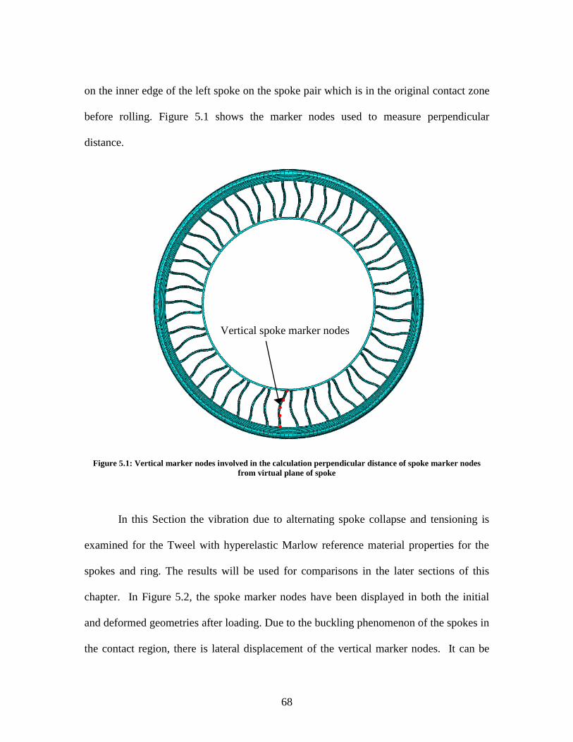
68
on the inner edge of the left spoke on the spoke pair which is in the original contact zone
before rolling. Figure 5.1 shows the marker nodes used to measure perpendicular
distance.
Figure 5.1: Vertical marker nodes involved in the calculation perpendicular distance of spoke marker nodes
from virtual plane of spoke
In this Section the vibration due to alternating spoke collapse and tensioning is
examined for the Tweel with hyperelastic Marlow reference material properties for the
spokes and ring. The results will be used for comparisons in the later sections of this
chapter. In Figure 5.2, the spoke marker nodes have been displayed in both the initial
and deformed geometries after loading. Due to the buckling phenomenon of the spokes in
the contact region, there is lateral displacement of the vertical marker nodes. It can be
Vertical spoke marker nodes

69
seen that the spoke curvature for the deformed geometry is much larger than the initial
geometry due to buckling. Since the spoke alternates between compression and tension
during rolling, the spoke length keeps varying. The time history of displacements of the
marker nodes are recorded for four revolutions during the steady rolling step (0.105 –
0.405 seconds).
Initial geometry
Deformed geometry
Figure 5.2: Vertical spoke marker nodes in both initial and deformed geometries of the Tweel
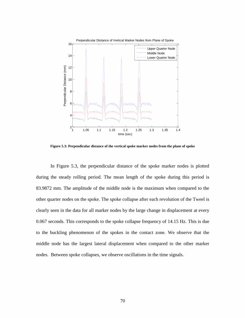
70
Figure 5.3: Perpendicular distance of the vertical spoke marker nodes from the plane of spoke
In Figure 5.3, the perpendicular distance of the spoke marker nodes is plotted
during the steady rolling period. The mean length of the spoke during this period is
83.9872 mm. The amplitude of the middle node is the maximum when compared to the
other quarter nodes on the spoke. The spoke collapse after each revolution of the Tweel is
clearly seen in the data for all marker nodes by the large change in displacement at every
0.067 seconds. This corresponds to the spoke collapse frequency of 14.15 Hz. This is due
to the buckling phenomenon of the spokes in the contact zone. We observe that the
middle node has the largest lateral displacement when compared to the other marker
nodes. Between spoke collapses, we observe oscillations in the time signals.
1 1.05 1.1 1.15 1.2 1.25 1.3 1.35 1.42
4
6
8
10
12
14
16
time (sec)
Perp
endic
ula
r D
ista
nce (
mm
)
Perpendicular Distance of Vertical Marker Nodes from Plane of Spoke
Upper Quarter Node
Middle Node
Lower Quarter Node

71
Figure 5.4: Magnitude of FFT with hamming window for perpendicular distance for middle vertical node.
Figure 5.4 is the magnitude of the FFT with hamming window and zero padding
for the middle vertical node perpendicular distance. There are two peaks that are
considered in this plot. The peak that occurs at 29 Hz is a multiple of the spoke collapse
frequency of 14.15 Hz. This frequency corresponds to the spoke collapse that occurs at
every 0.067 seconds. Since this peak is a result of the spoke collapsing due to the
buckling phenomenon, it will not be considered for analyzing spoke vibration. The
amplitudes below approximately 100 Hz are considered the response from the spoke
collapse frequency and associated harmonics. Above approximately 100 Hz, the
amplitudes due to spoke vibration are very small. The peak that will be considered is the
one that occurs at 335 Hz. These small peaks near 335 Hz result from the oscillations in
the perpendicular distance time signal during the tension phase of the spoke. The root-
0 100 200 300 400 500 600 700 8000
50
100
150
200
250
300
X: 334.8
Y: 5.159
Magnitude of Hamming Window with zero padding
Frequency f (Hz)
|X|
X: 29.65
Y: 265.5

72
mean-square (RMS) of the FFT amplitudes for the middle node in the reference model
over a frequency range between 200 to 800 Hz is 1.4246. RMS gives a measure of the
overall vibration amplitude for frequency region of interest. The RMS of a set of N,
amplitude values is computed from,
2
1
.N
i
i
xRMS
N
5.2 Vibration due to ground interaction
One of the main sources of vibration is due to the interaction between the Tweel
and the ground while rolling. This is estimated by observing the ground reaction force
time signal during rolling and the corresponding FFT frequency response of the zero
mean signal. The results in this Section are given for the reference Marlow model and
will be used for comparisons in the later sections of this chapter.
Figure 5.5: Reaction force exerted by the ground on the Tweel
1 1.05 1.1 1.15 1.2 1.25 1.3
310
320
330
340
350
360
370
380
390
400
410
time (sec)
daN
Ground Reaction Force

73
Figure 5.5 gives the reaction force interaction time signal between the rigid flat
ground and the Tweel during steady rolling. The mean value of the ground reaction force
for the reference model during steady rolling is recorded as 367.6758 daN. Low
frequency oscillations in the signal with period of approximately 0.067 seconds
correspond to the spoke collapse frequency for one complete revolution of the Tweel.
Figure 5.6: FFT amplitude for the ground reaction force
In Figure 5.6, the highest FFT amplitude peak occurs at the spoke collapse
frequency of 14.15 Hz. Other large FFT amplitude peaks occur at 369.3 Hz and 738.7 Hz.
The first peak at 369.3 Hz corresponds to the spoke pair passing frequency which
depends on the angular velocity with which the Tweel is rolling and the number of
spokes (recall the Tweel considered has 25 spoke pairs). The vibration at this frequency
0 100 200 300 400 500 600 700 800 900 10000
2000
4000
6000
8000
10000
12000
X: 738.7
Y: 1510
zero mean signal
Magnitude
Frequency (Hz)
X: 369.3
Y: 912.4

74
may be due to the discrete stiffness of the spokes [5]. Also, the peak at 738.7 Hz
corresponds to the single spoke passing frequency which is twice the spoke pair passing
frequency. The RMS of the ground reaction force amplitudes over a frequency range of
200 to 1000 Hz is 94.
5.3 Effects of Material Properties on Vibration during steady state rolling
A material study is performed in the following sections of this chapter. In this
study, the spoke and the ground interaction vibration is analyzed and compared using
corresponding FFT amplitude RMS values. The following sets of results are reported for
the ring material changed to Mooney Rivlin and Neo Hookean while keeping the same
Marlow material on the spokes.
5.3.1 Mooney Rivlin model for ring with unchanged shear modulus
Figure 5.7: Perpendicular distance of spoke marker nodes from plane of spoke.
1 1.05 1.1 1.15 1.2 1.25 1.3 1.35 1.42
4
6
8
10
12
14
16
time (sec)
Perp
endic
ula
r D
ista
nce (
mm
)
Perpendicular Distance of Vertical Marker Nodes from Plane of Spoke
Upper Quarter Node
Middle Node
Lower Quarter Node

75
Figure 5.8: Magnitude of FFT amplitude of perpendicular distance for middle node.
From Figure 5.7 and Figure 5.8, the RMS of the FFT amplitudes for spoke
vibration is 1.5971. The average spoke length is 83.9813 mm. The peak amplitude for
spoke vibration occurs at 325 Hz.
0 100 200 300 400 500 600 700 8000
50
100
150
200
250
300Magnitude of Hamming Window with zero padding
Frequency f (Hz)
|X|
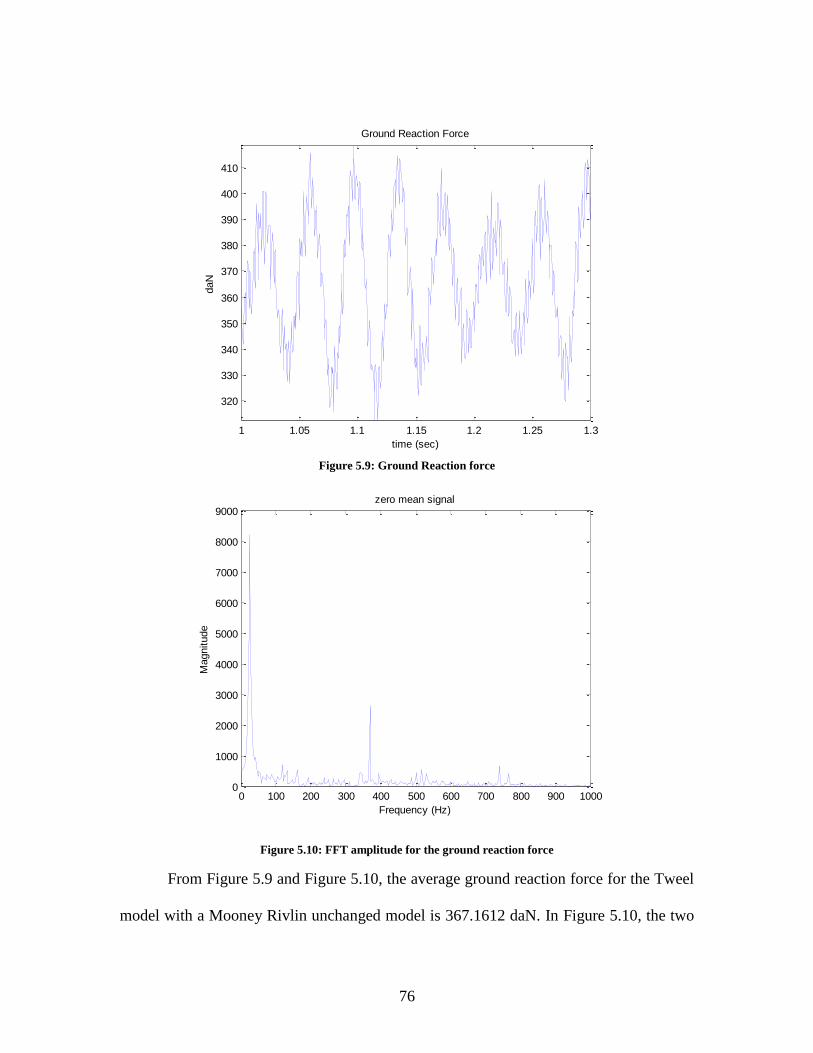
76
Figure 5.9: Ground Reaction force
Figure 5.10: FFT amplitude for the ground reaction force
From Figure 5.9 and Figure 5.10, the average ground reaction force for the Tweel
model with a Mooney Rivlin unchanged model is 367.1612 daN. In Figure 5.10, the two
1 1.05 1.1 1.15 1.2 1.25 1.3
320
330
340
350
360
370
380
390
400
410
time (sec)
daN
Ground Reaction Force
0 100 200 300 400 500 600 700 800 900 10000
1000
2000
3000
4000
5000
6000
7000
8000
9000zero mean signal
Magnitude
Frequency (Hz)

77
peaks that are considered the spoke pair passing frequencies occur at 369 Hz and 739 Hz.
The RMS of the FFT amplitude for the ground reaction force over a frequency range
from 200 Hz to 1000 Hz is 130.
5.3.2 Shear modulus of Mooney Rivlin model for the ring is reduced by 25%
From Figure 5.11 and Figure 5.12, the RMS of the FFT amplitudes for spoke
vibration is 2.4242. The average spoke length is 83.9872 mm. The peak amplitude for
spoke vibration occurs at 322 Hz.
Figure 5.11: Perpendicular distance of vertical marker nodes from plane of spoke
1 1.05 1.1 1.15 1.2 1.25 1.3 1.35 1.42
4
6
8
10
12
14
16
time (sec)
Perp
endic
ula
r D
ista
nce (
mm
)
Perpendicular Distance of Vertical Marker Nodes from Plane of Spoke
Upper Quarter Node
Middle Node
Lower Quarter Node

78
Figure 5.12: Magnitude of FFT amplitude of perpendicular distance for the middle node
From Figure 5.13, the average ground reaction force for the Tweel model with a
Mooney Rivlin reduced model is 365.6308 daN. In Figure 5.14, the two peaks that are
considered occur at 370 and 740 Hz. The RMS of the FFT amplitude for the ground
reaction force over a frequency range from 200 Hz to 1000 Hz is 313.
0 100 200 300 400 500 600 700 8000
50
100
150
200
250
300Magnitude of Hamming Window with zero padding
Frequency f (Hz)
|X|
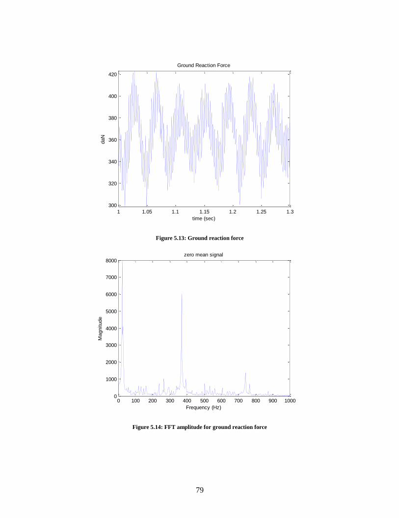
79
Figure 5.13: Ground reaction force
Figure 5.14: FFT amplitude for ground reaction force
1 1.05 1.1 1.15 1.2 1.25 1.3
300
320
340
360
380
400
420
time (sec)
daN
Ground Reaction Force
0 100 200 300 400 500 600 700 800 900 10000
1000
2000
3000
4000
5000
6000
7000
8000zero mean signal
Magnitude
Frequency (Hz)

80
5.3.3 Shear modulus of the Mooney Rivlin model for the ring is increased by 25%
From Figure 5.15 and Figure 5.16, the RMS of the FFT amplitudes for spoke
vibration is 1.7761. The average spoke length is 83.9246 mm. The peak amplitude for
spoke vibration occurs at 328 Hz.
Figure 5.15: Perpendicular distance of vertical marker nodes from plane of spoke
1 1.05 1.1 1.15 1.2 1.25 1.3 1.35 1.42
4
6
8
10
12
14
16
time (sec)
Perp
endic
ula
r D
ista
nce (
mm
)
Perpendicular Distance of Vertical Marker Nodes from Plane of Spoke
Upper Quarter Node
Middle Node
Lower Quarter Node

81
Figure 5.16: Magnitude of FFT amplitudes of perpendicular distance for the middle node
0 100 200 300 400 500 600 700 8000
50
100
150
200
250
300Magnitude of Hamming Window with zero padding
Frequency f (Hz)
|X|

82
In Figure 5.17, the average ground reaction force for the Tweel with a Mooney
Rivlin increased model is 367.7807 daN. In Figure 5.18, the two important peaks occur at
frequencies 343 and 765 Hz. The RMS of the FFT amplitudes for the ground reaction
force over a frequency range from 200 Hz to 1000 Hz is 71.
Figure 5.17: Reaction force exerted by the ground on the Tweel
1 1.05 1.1 1.15 1.2 1.25 1.3
300
320
340
360
380
400
420
time (sec)
daN
Ground Reaction Force
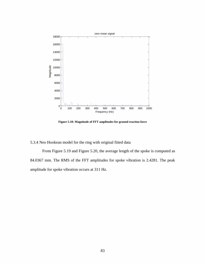
83
Figure 5.18: Magnitude of FFT amplitudes for ground reaction force
5.3.4 Neo Hookean model for the ring with original fitted data
From Figure 5.19 and Figure 5.20, the average length of the spoke is computed as
84.0367 mm. The RMS of the FFT amplitudes for spoke vibration is 2.4281. The peak
amplitude for spoke vibration occurs at 311 Hz.
0 100 200 300 400 500 600 700 800 900 10000
2000
4000
6000
8000
10000
12000
14000
16000
18000zero mean signal
Magnitude
Frequency (Hz)

84
Figure 5.19: Perpendicular distance of vertical spoke marker nodes from plane of spoke
Figure 5.20: Magnitude of FFT amplitudes of perpendicular distance for the middle node
1 1.05 1.1 1.15 1.2 1.25 1.3 1.35 1.42
4
6
8
10
12
14
16
time (sec)
Perp
endic
ula
r D
ista
nce (
mm
)
Perpendicular Distance of Vertical Marker Nodes from Plane of Spoke
Upper Quarter Node
Middle Node
Lower Quarter Node
0 100 200 300 400 500 600 700 8000
50
100
150
200
250
300Magnitude of Hamming Window with zero padding
Frequency f (Hz)
|X|

85
From Figure 5.21, the average reaction force is 366.4391 daN. In Figure 5.22, the
two important peaks occur at 371 Hz and 742 Hz. The RMS of the FFT amplitudes for
ground reaction force over a range from 200 Hz to 1000 Hz is computed as 213.
Figure 5.21: Ground reaction force
1 1.05 1.1 1.15 1.2 1.25 1.3
340
350
360
370
380
390
time (sec)
daN
Ground Reaction Force

86
Figure 5.22: Magnitude of FFT amplitudes for ground reaction force
5.3.5 Shear modulus of the Neo Hookean model for the ring is reduced by 25%
From Figure 5.23 and Figure 5.24, the average length of the spoke is 84.0566
mm. The peak amplitude occurs at 372 Hz. The RMS of the FFT amplitude of spoke
vibration for the middle node is 6.2373. In this case, there is clearly a large amplitude
vibration in the spokes during the tension phase.
0 100 200 300 400 500 600 700 800 900 10000
500
1000
1500
2000
2500
3000zero mean signal
Magnitude
Frequency (Hz)

87
Figure 5.23: Perpendicular distance of vertical spoke marker nodes from plane of spoke
Figure 5.24: Magnitude of FFT amplitudes of perpendicular distance for middle node
1 1.05 1.1 1.15 1.2 1.25 1.3 1.35 1.42
4
6
8
10
12
14
16
18
time (sec)
Perp
endic
ula
r D
ista
nce (
mm
)
Perpendicular Distance of Vertical Marker Nodes from Plane of Spoke
Upper Quarter Node
Middle Node
Lower Quarter Node
0 100 200 300 400 500 600 700 8000
50
100
150
200
250
300Magnitude of Hamming Window with zero padding
Frequency f (Hz)
|X|

88
In Figure 5.25, the average ground reaction force is 366.4078 daN. In Figure 5.26,
the peak amplitudes occur at frequencies 373 and 742 Hz. The RMS of the FFT
amplitude for ground reaction force is 479. The vibration amplitudes for ground force
interaction much larger for this material property in the ring. Recall for this material with
reduced shear modulus, the slope of the vertical load versus displacement was reduced
indicating a soft stiffness.
Figure 5.25: Reaction force exerted by the ground on the Tweel
1 1.05 1.1 1.15 1.2 1.25 1.3
330
340
350
360
370
380
390
400
410
420
time (sec)
daN
Ground Reaction Force
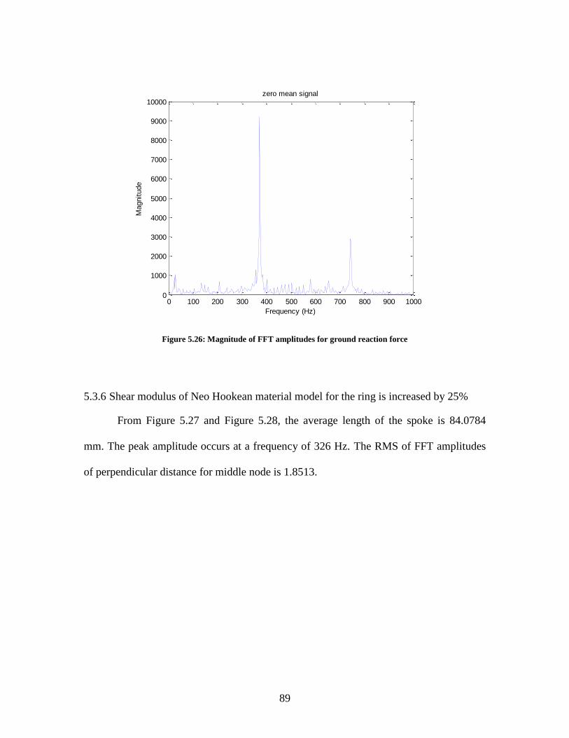
89
Figure 5.26: Magnitude of FFT amplitudes for ground reaction force
5.3.6 Shear modulus of Neo Hookean material model for the ring is increased by 25%
From Figure 5.27 and Figure 5.28, the average length of the spoke is 84.0784
mm. The peak amplitude occurs at a frequency of 326 Hz. The RMS of FFT amplitudes
of perpendicular distance for middle node is 1.8513.
0 100 200 300 400 500 600 700 800 900 10000
1000
2000
3000
4000
5000
6000
7000
8000
9000
10000zero mean signal
Magnitude
Frequency (Hz)

90
Figure 5.27: Perpendicular distance of spoke marker nodes from plane of spoke
Figure 5.28: Magnitude of FFT amplitudes of perpendicular distance for middle node
1 1.05 1.1 1.15 1.2 1.25 1.3 1.35 1.42
4
6
8
10
12
14
16
time (sec)
Perp
endic
ula
r D
ista
nce (
mm
)
Perpendicular Distance of Vertical Marker Nodes from Plane of Spoke
Upper Quarter Node
Middle Node
Lower Quarter Node
0 100 200 300 400 500 600 700 8000
50
100
150
200
250
300Magnitude of Hamming Window with zero padding
Frequency f (Hz)
|X|
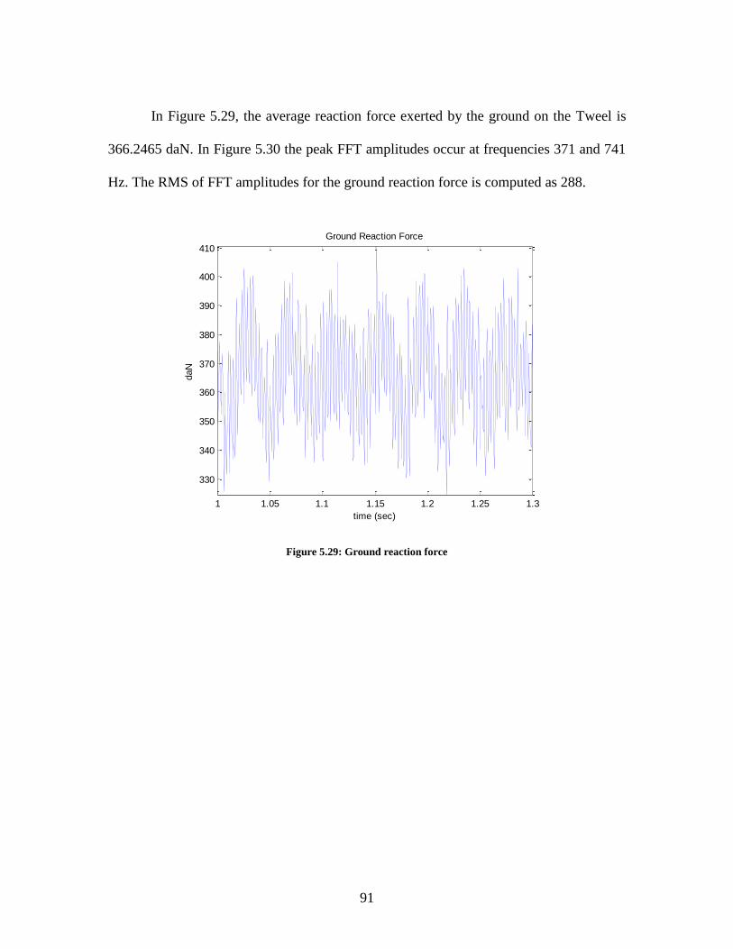
91
In Figure 5.29, the average reaction force exerted by the ground on the Tweel is
366.2465 daN. In Figure 5.30 the peak FFT amplitudes occur at frequencies 371 and 741
Hz. The RMS of FFT amplitudes for the ground reaction force is computed as 288.
Figure 5.29: Ground reaction force
1 1.05 1.1 1.15 1.2 1.25 1.3
330
340
350
360
370
380
390
400
410
time (sec)
daN
Ground Reaction Force
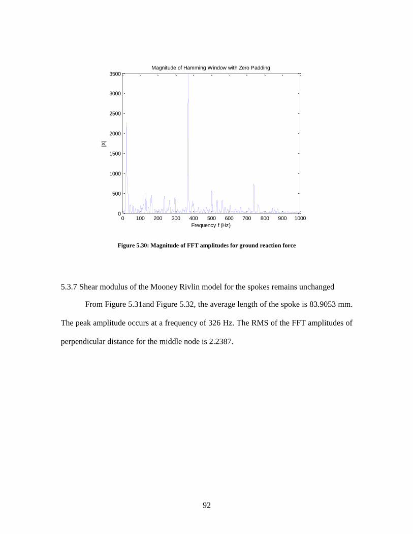
92
Figure 5.30: Magnitude of FFT amplitudes for ground reaction force
5.3.7 Shear modulus of the Mooney Rivlin model for the spokes remains unchanged
From Figure 5.31and Figure 5.32, the average length of the spoke is 83.9053 mm.
The peak amplitude occurs at a frequency of 326 Hz. The RMS of the FFT amplitudes of
perpendicular distance for the middle node is 2.2387.
0 100 200 300 400 500 600 700 800 900 10000
500
1000
1500
2000
2500
3000
3500Magnitude of Hamming Window with Zero Padding
Frequency f (Hz)
|X|

93
Figure 5.31: Perpendicular distance of vertical marker nodes from plane of spoke
Figure 5.32: Magnitude of FFT amplitudes of perpendicular distance for the middle node
1 1.05 1.1 1.15 1.2 1.25 1.3 1.35 1.42
4
6
8
10
12
14
16
18
time (sec)
Perp
endic
ula
r D
ista
nce (
mm
)
Perpendicular Distance of Vertical Marker Nodes from Plane of Spoke
Upper Quarter Node
Middle Node
Lower Quarter Node
0 100 200 300 400 500 600 700 8000
50
100
150
200
250
300
350
400Magnitude of Hamming Window with zero padding
Frequency f (Hz)
|X|
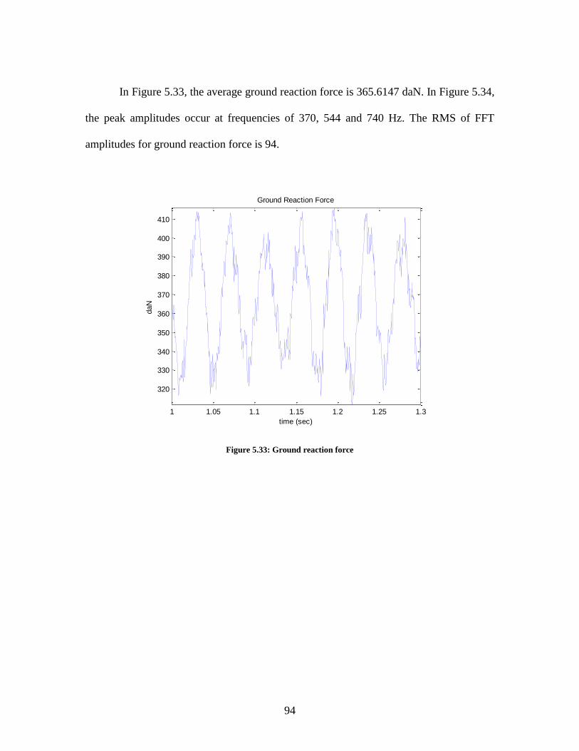
94
In Figure 5.33, the average ground reaction force is 365.6147 daN. In Figure 5.34,
the peak amplitudes occur at frequencies of 370, 544 and 740 Hz. The RMS of FFT
amplitudes for ground reaction force is 94.
Figure 5.33: Ground reaction force
1 1.05 1.1 1.15 1.2 1.25 1.3
320
330
340
350
360
370
380
390
400
410
time (sec)
daN
Ground Reaction Force

95
Figure 5.34: Magnitude of FFT amplitude for ground reaction force
5.3.8 Shear modulus of Mooney Rivlin material model for the spokes is reduced by 25%
From Figure 5.35 and Figure 5.36, the average length of the spoke is 83.8640
mm. The peak amplitude occurs at a frequency of 223 Hz. The RMS of FFT amplitude of
perpendicular distance for middle node is 2.4583.
0 100 200 300 400 500 600 700 800 900 10000
2000
4000
6000
8000
10000
12000zero mean signal
Magnitude
Frequency (Hz)
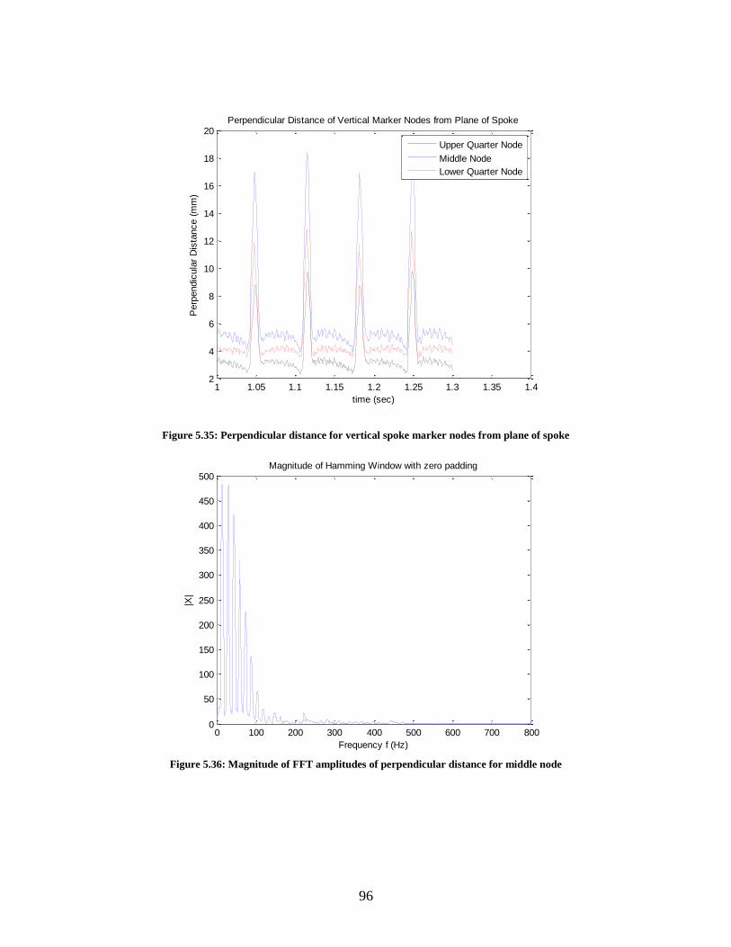
96
Figure 5.35: Perpendicular distance for vertical spoke marker nodes from plane of spoke
Figure 5.36: Magnitude of FFT amplitudes of perpendicular distance for middle node
1 1.05 1.1 1.15 1.2 1.25 1.3 1.35 1.42
4
6
8
10
12
14
16
18
20
time (sec)
Perp
endic
ula
r D
ista
nce (
mm
)
Perpendicular Distance of Vertical Marker Nodes from Plane of Spoke
Upper Quarter Node
Middle Node
Lower Quarter Node
0 100 200 300 400 500 600 700 8000
50
100
150
200
250
300
350
400
450
500Magnitude of Hamming Window with zero padding
Frequency f (Hz)
|X|

97
In Figure 5.37, the average ground reaction force is 366.7383 daN. In Figure 5.38,
the peak amplitudes occur at frequencies of 369, 534 and 772 Hz. The RMS of FFT
amplitudes for ground reaction force is 141.
Figure 5.37: Reaction force exerted by the ground on the Tweel
1 1.05 1.1 1.15 1.2 1.25 1.3
330
340
350
360
370
380
390
400
410
time (sec)
daN
Ground Reaction Force
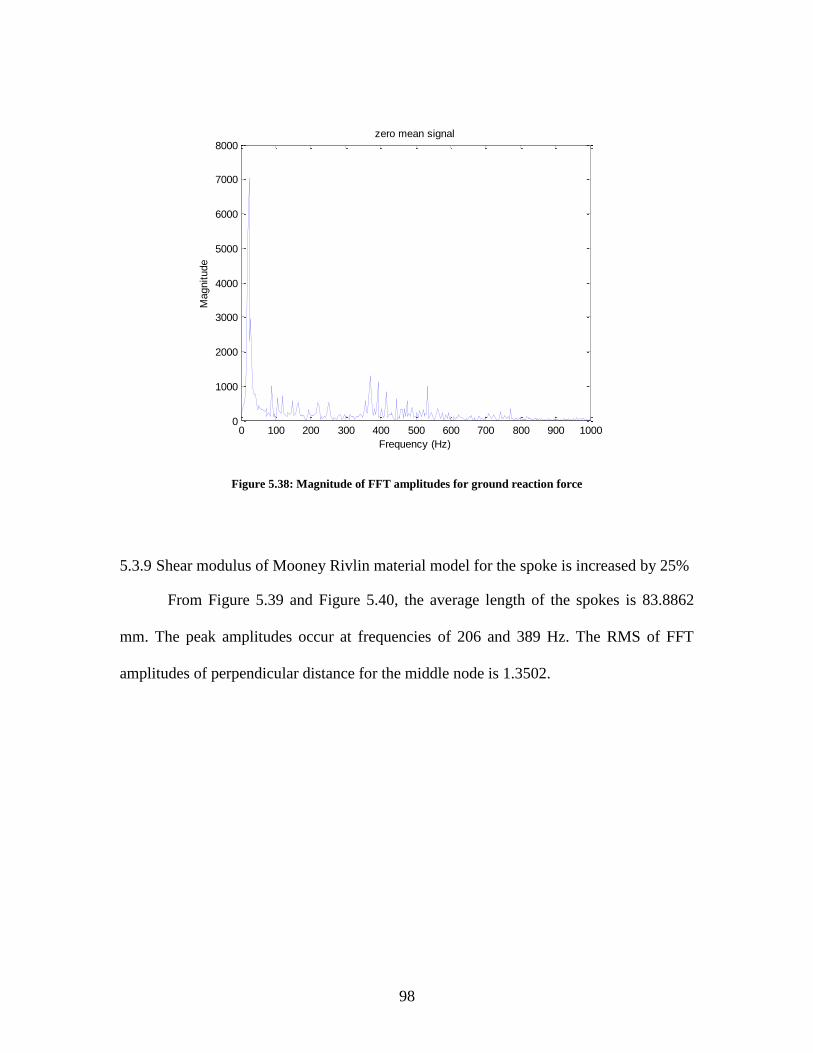
98
Figure 5.38: Magnitude of FFT amplitudes for ground reaction force
5.3.9 Shear modulus of Mooney Rivlin material model for the spoke is increased by 25%
From Figure 5.39 and Figure 5.40, the average length of the spokes is 83.8862
mm. The peak amplitudes occur at frequencies of 206 and 389 Hz. The RMS of FFT
amplitudes of perpendicular distance for the middle node is 1.3502.
0 100 200 300 400 500 600 700 800 900 10000
1000
2000
3000
4000
5000
6000
7000
8000zero mean signal
Magnitude
Frequency (Hz)
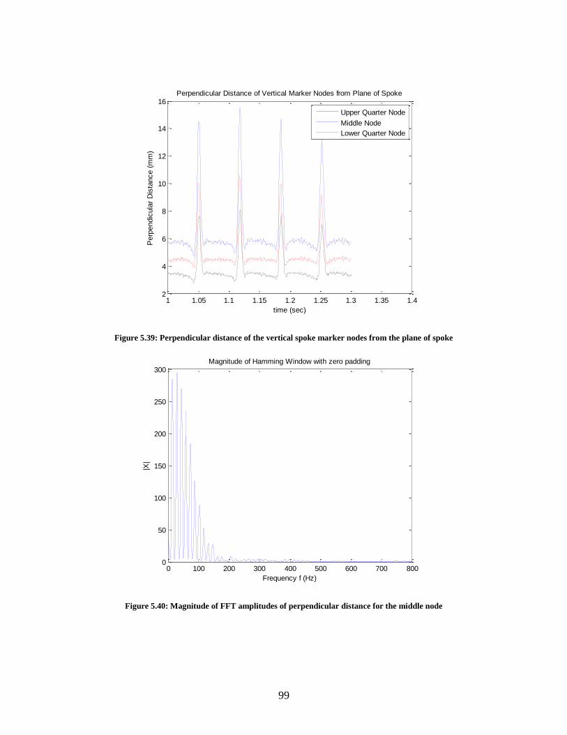
99
Figure 5.39: Perpendicular distance of the vertical spoke marker nodes from the plane of spoke
Figure 5.40: Magnitude of FFT amplitudes of perpendicular distance for the middle node
1 1.05 1.1 1.15 1.2 1.25 1.3 1.35 1.42
4
6
8
10
12
14
16
time (sec)
Perp
endic
ula
r D
ista
nce (
mm
)
Perpendicular Distance of Vertical Marker Nodes from Plane of Spoke
Upper Quarter Node
Middle Node
Lower Quarter Node
0 100 200 300 400 500 600 700 8000
50
100
150
200
250
300Magnitude of Hamming Window with zero padding
Frequency f (Hz)
|X|
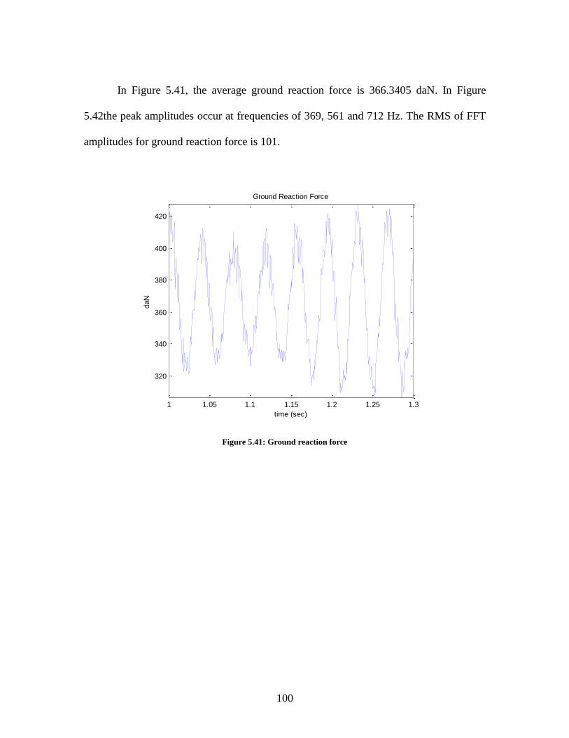
100
In Figure 5.41, the average ground reaction force is 366.3405 daN. In Figure
5.42the peak amplitudes occur at frequencies of 369, 561 and 712 Hz. The RMS of FFT
amplitudes for ground reaction force is 101.
Figure 5.41: Ground reaction force
1 1.05 1.1 1.15 1.2 1.25 1.3
320
340
360
380
400
420
time (sec)
daN
Ground Reaction Force
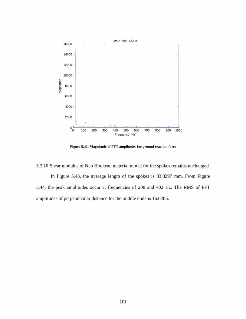
101
Figure 5.42: Magnitude of FFT amplitudes for ground reaction force
5.3.10 Shear modulus of Neo Hookean material model for the spokes remains unchanged
In Figure 5.43, the average length of the spokes is 83.8297 mm. From Figure
5.44, the peak amplitudes occur at frequencies of 208 and 402 Hz. The RMS of FFT
amplitudes of perpendicular distance for the middle node is 16.0285.
0 100 200 300 400 500 600 700 800 900 10000
2000
4000
6000
8000
10000
12000
14000
16000zero mean signal
Magnitude
Frequency (Hz)
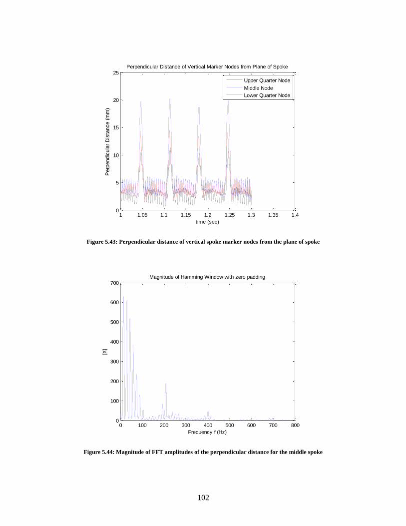
102
Figure 5.43: Perpendicular distance of vertical spoke marker nodes from the plane of spoke
Figure 5.44: Magnitude of FFT amplitudes of the perpendicular distance for the middle spoke
1 1.05 1.1 1.15 1.2 1.25 1.3 1.35 1.40
5
10
15
20
25
time (sec)
Perp
endic
ula
r D
ista
nce (
mm
)
Perpendicular Distance of Vertical Marker Nodes from Plane of Spoke
Upper Quarter Node
Middle Node
Lower Quarter Node
0 100 200 300 400 500 600 700 8000
100
200
300
400
500
600
700Magnitude of Hamming Window with zero padding
Frequency f (Hz)
|X|

103
For ground interaction, from Figure 5.45, the average ground reaction force is
366.6618 daN. In Figure 5.46, the peak amplitudes occur at frequencies of 372 and 764
Hz. The RMS of FFT amplitudes for ground reaction force is 801.
Figure 5.45: Reaction force exerted by the ground on the Tweel
1 1.05 1.1 1.15 1.2 1.25 1.3
280
300
320
340
360
380
400
420
440
time (sec)
daN
Ground Reaction Force

104
Figure 5.46: Magnitude of FFT amplitudes for ground reaction force
5.3.11 Shear modulus of the Neo Hookean model for the spokes is reduced by 25%
From Figure 5.47 and Figure 5.48, the average length of the spoke is 83.7442
mm. The RMS of FFT amplitudes of perpendicular distance for the middle node is
5.9097. The peak amplitude occurs at a frequency of 360 Hz.
0 100 200 300 400 500 600 700 800 900 10000
1000
2000
3000
4000
5000
6000
7000
8000
9000
10000Magnitude of Hamming Window with Zero Padding
Frequency f (Hz)
|X|

105
Figure 5.47: Perpendicular distance of the vertical marker nodes from plane of spoke
Figure 5.48: Magnitude of FFT amplitudes of perpendicular distance for the middle node
1 1.05 1.1 1.15 1.2 1.25 1.3 1.35 1.40
5
10
15
20
25
time (sec)
Perp
endic
ula
r D
ista
nce (
mm
)
Perpendicular Distance of Vertical Marker Nodes from Plane of Spoke
Upper Quarter Node
Middle Node
Lower Quarter Node
0 100 200 300 400 500 600 700 8000
100
200
300
400
500
600
700
800Magnitude of Hamming Window with zero padding
Frequency f (Hz)
|X|

106
For the ground interaction, in Figure 5.49, the average ground reaction force is
365.0709 daN. In Figure 5.50, the peak amplitudes occur at frequencies of 374 and 746
Hz. The RMS of FFT amplitudes for ground reaction force is 472.
Figure 5.49: Ground reaction force
1 1.05 1.1 1.15 1.2 1.25 1.3
260
280
300
320
340
360
380
400
420
440
time (sec)
daN
Ground Reaction Force

107
Figure 5.50: Magnitude of FFT amplitudes for ground reaction force
5.3.12 Shear modulus of Neo Hookean model for the spokes is increased by 25%
In Figure 5.51 and Figure 5.52, for spoke vibration, the average length of the
spokes is 83.9044 mm. The peak amplitudes occur at frequencies of 238 and 282 Hz. The
RMS of the FFT amplitudes of perpendicular distance for the middle node is 3.757.
0 100 200 300 400 500 600 700 800 900 10000
1000
2000
3000
4000
5000
6000
7000
8000
9000zero mean signal
Magnitude
Frequency (Hz)

108
Figure 5.51: Perpendicular distance of the vertical spoke marker nodes
Figure 5.52: magnitude of FFT amplitudes of perpendicular distance for the middle node on the spoke edge
1 1.05 1.1 1.15 1.2 1.25 1.3 1.35 1.42
4
6
8
10
12
14
16
18
20
time (sec)
Perp
endic
ula
r D
ista
nce (
mm
)
Perpendicular Distance of Vertical Marker Nodes from Plane of Spoke
Upper Quarter Node
Middle Node
Lower Quarter Node
0 100 200 300 400 500 600 700 8000
100
200
300
400
500
600Magnitude of Hamming Window with zero padding
Frequency f (Hz)
|X|

109
For ground interaction, in Figure 5.53, the average ground reaction force is
365.7203 daN. In Figure 5.54, the peak amplitudes occur at frequencies of 371, 484 and
764 Hz. The RMS of FFT amplitudes for the ground reaction force is 204.
Figure 5.53: Reaction force exerted by the ground on the Tweel
1 1.05 1.1 1.15 1.2 1.25 1.3
330
340
350
360
370
380
390
400
time (sec)
daN
Ground Reaction Force

110
Figure 5.54: Magnitude of FFT amplitudes for ground reaction force.
5.4 Observations
In this section, the RMS values of the FFT amplitudes for spoke vibration and
ground interaction vibration summarized and compared in this section. Four bar charts
have been provided for both spoke vibration and ground vibration.
0 100 200 300 400 500 600 700 800 900 10000
500
1000
1500
2000
2500
3000
3500
4000
4500
5000zero mean signal
Magnitude
Frequency (Hz)

111
5.4.1 Comparison of RMS values of FFT amplitudes for Spoke Vibration
In Figure 5.55, there are two sets of RMS values. The first set „Ring‟ refers to the
Tweel models with unchanged Mooney Rivlin and unchanged Neo Hookean models for
the ring. Likewise, „Spoke‟ refers to the Tweel models with unchanged Mooney Rivlin
and unchanged Neo Hookean models for the spokes.
Figure 5.55: RMS of FFT amplitudes of perpendicular distance from virtual spoke plane for reference and
unchanged models
The RMS of FFT amplitude for the reference Marlow model is 1.42. When an
unchanged Mooney Rivlin material model was used for the ring instead of Marlow, the
RMS value increased to 1.60. The RMS of FFT amplitude further increased to 2.43 when
an unchanged Neo Hookean material model was used for the ring instead of Marlow.
1.42
1.42
1.60
2.24
2.43
16.03
Ring
Spoke
RMS of FFT amplitudes of Perpendicular Distance
Neo-Hookean Mooney-Rivlin Marlow

112
Similarly, when an unchanged Mooney Rivlin material model was used for the
spokes, the RMS value increased from 1.42 to 2.24. There was a drastic increase in the
RMS value when an unchanged Neo Hookean material model was used for the spokes.
The RMS value increased to 16.03.
The general trend shown is that the vibration amplitude in the spokes increases
when the Marlow properties are changed to either the fitted Mooney Rivlin or Neo
Hookean models, with the Neo Hookean model giving the largest vibration amplitudes,
especially in the case of changes in spoke properties. It also appears from these results
that changes to spoke material properties have a more significant influence on spoke
vibration when compared to changes in ring properties.
Figure 5.56: RMS of FFT amplitudes for different Mooney Rivlin and Neo Hookean models
1.60
2.43
2.24
16.03
1.78
1.85
1.35
3.76
2.42
6.24
2.46
5.91
Mooney-Rivlin for the ring
Neo-Hookean for the ring
Mooney-Rivlin for the spokes
Neo-Hookean for the spokes
RMS of FFT amplitudes of Perpendicular Distance
minus 25% plus 25% Unchanged

113
In Figure 5.56, four sets of RMS values have been provided. „Mooney Rivlin for
the ring‟ refers to all the Tweel models with different Mooney Rivlin models for the ring.
A similar explanation can be given for the rest of the 3 sets of RMS values.
When a Mooney Rivlin model with reduced shear modulus for the ring was used,
the RMS value increased to 2.42 from 1.60. The RMS value increased to 1.78 from 1.60
when a Mooney Rivlin with increased shear modulus for the ring was used.
When Neo Hookean material models were used for the ring, the RMS value for
the Tweel model with an unchanged Neo Hookean model was 2.43. When the shear
modulus was increased by 25%, the RMS value reduced to 1.85. But when the shear
modulus was reduced to 25%, the RMS value increased to 6.24.
On changing the spoke material models to Mooney Rivlin, the Tweel model with
an unchanged Mooney Rivlin model for the spokes had a RMS value of 2.24. When the
shear modulus was reduced by 25%, the RMS value increased to 2.46. When the shear
modulus was increased by 25%, the RMS value reduced to 1.35 from 2.43.
Finally, when Neo Hookean material models were used for the spoke, the Tweel
model with an unchanged Neo Hookean material model had a RMS value of 16.03. But
when the shear modulus was reduced by 25%, the RMS value decreased 5.91. The RMS
value dropped further down to 3.75 when the shear modulus was increased by 25%.
A general trend found in these results when comparing the extreme limits of plus
and minus 25% change, is that when the shear modulus is decreased, the spoke vibration
increases. Conversely, when the shear modulus is increased from -25% to +25%, the
spoke vibration decreases. However, it should be noted that in the case of the unchanged

114
Mooney Rivlin model for the ring, the unchanged gave the smallest amplitude when
compared to both the plus and minus extreme limits tested, thus implying that there is an
optimal value somewhere between the limits. Another instance where an optimal value
occurs can be seen in the Neo Hookean model for the spokes, where the unchanged spoke
vibration amplitude was higher than both the plus and minus stiffness limits. Note also
that the unchanged Neo Hookean model for the spokes had the largest amplitude when
compared to all models. However, it should be noted that in the case of the unchanged
Mooney Rivlin model for the ring, the unchanged gave the smallest amplitude when
compared to both the plus and minus extreme limits tested, thus implying that there is an
optimal value somewhere between the limits. Another instance where an optimal value
occurs can be seen in the Neo Hookean model for the spokes, where the unchanged spoke
vibration amplitude was higher than both the plus and minus stiffness limits. Note also
that the unchanged Neo Hookean model for the spokes had the largest amplitude when
compared to all models.
5.4.2 Comparison of RMS values of FFT amplitudes for Ground Interaction Vibration
In Figure 5.57, two sets of RMS values have been provided. Similar to the spoke
vibration, „Ring‟ refers to all the Tweel models with unchanged Mooney Rivlin and Neo
Hookean models for the ring instead of Marlow. A similar explanation can be given for
the second set named „Spoke‟.
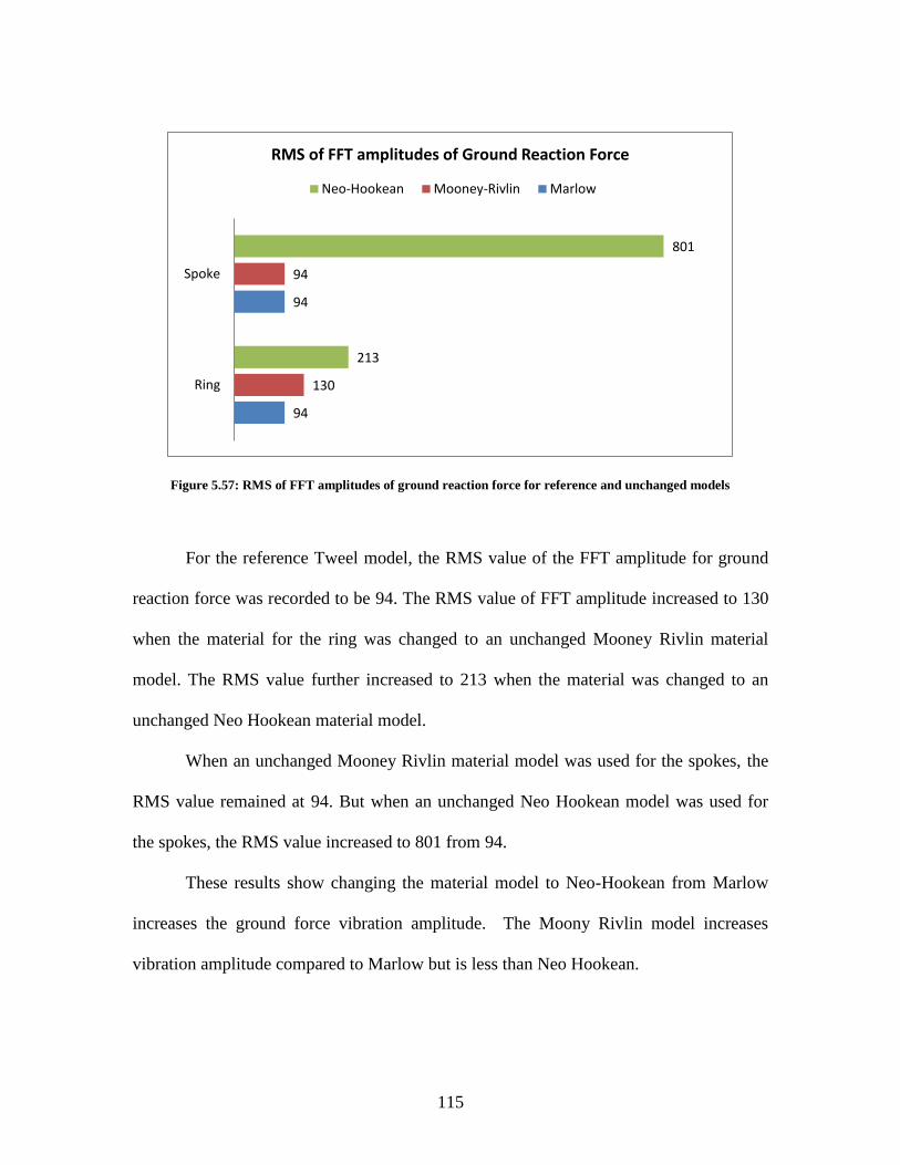
115
Figure 5.57: RMS of FFT amplitudes of ground reaction force for reference and unchanged models
For the reference Tweel model, the RMS value of the FFT amplitude for ground
reaction force was recorded to be 94. The RMS value of FFT amplitude increased to 130
when the material for the ring was changed to an unchanged Mooney Rivlin material
model. The RMS value further increased to 213 when the material was changed to an
unchanged Neo Hookean material model.
When an unchanged Mooney Rivlin material model was used for the spokes, the
RMS value remained at 94. But when an unchanged Neo Hookean model was used for
the spokes, the RMS value increased to 801 from 94.
These results show changing the material model to Neo-Hookean from Marlow
increases the ground force vibration amplitude. The Moony Rivlin model increases
vibration amplitude compared to Marlow but is less than Neo Hookean.
94
94
130
94
213
801
Ring
Spoke
RMS of FFT amplitudes of Ground Reaction Force
Neo-Hookean Mooney-Rivlin Marlow

116
Figure 5.58: RMS of FFT amplitudes for different Mooney Rivlin and Neo Hookean models
In Figure 5.58, four sets of RMS values have been provided. In the first set, the
material for the ring is changed to an unchanged, reduced and an increased Mooney
Rivlin model. A similar explanation is valid for the other three sets.
When Mooney Rivlin is used for the ring, the RMS for the unchanged model was
130. The RMS value for the Tweel with a Mooney Rivlin model whose shear modulus is
reduced by 25% increased to 313 from 130. But when the shear modulus is increased by
25%, the RMS value of the FFT amplitudes decreased to 71.
Considering Neo Hookean for the ring, the unchanged model had a RMS value of
213. When the shear modulus is reduced by 25%, the RMS value increased to 479. The
RMS value increased to 288 when the shear modulus was increased by 25%.
When Mooney Rivlin was used for the spokes, the RMS value for the unchanged
model was recorded to be 94. When the shear modulus was reduced by 25%, the RMS
130
213
94
801
71
288
101
204
313
479
141
472
Mooney-Rivlin for the ring
Neo-Hookean for the ring
Mooney-Rivlin for the spokes
Neo-Hookean for the spokes
RMS of FFT amplitudes for Ground Reaction Force
minus 25% plus 25% Unchanged

117
value increased to 141 from 94. But when the shear modulus was increased by 25%, the
RMS value increased to 101 from 94.
Considering Neo Hookean for the spokes, the unchanged model‟s RMS value was
801. When the shear modulus was reduced by 25%, the RMS value decreased to 472
from 801. The RMS value further decreased to 204 from 801 when the shear modulus
was increased by 25%.
The results show that decreasing the shear modulus to -25% increased ground
force vibration compared to unchanged and increased modulus. Increasing the shear
modulus increased the ground force vibration when compared to unchanged Mooney-
Rivlin for the spokes and Neo-Hookean for the ring but decreased vibration in the other
cases. Similar to the spoke vibration, the Neo Hookean unchanged for the spokes gives
the largest vibration amplitude.
118
CHAPTER SIX- EFFECTS OF CHANGING MATERIAL PROPERTIES ON ENERGY
LOSS FROM IMPACT ROLLING OVER OBSTACLES
In Chapter One, the four critical characteristics of the pneumatic tire identified in
[1] have been explained. A major advantage of the pneumatic tire over a rigid wheel
comes from its behavior when traversing obstacles. In [1], it was shown that a pneumatic
tire gave less Kinetic energy loss when compared with a rigid wheel with the same mass
and moment of inertia properties when rolled over an obstacle. In [1], a particular
Tweel™ model with the same secant stiffness at the applied load, mass, moment of
inertia and initial velocity as a typical pneumatic wheel model was constructed. Upon
rolling the Tweel and the pneumatic tire over an obstacle, it was seen that the reduction in
hub velocity of the Tweel after impacting the obstacle was lesser than the pneumatic tire.
For this study, the radius used was 0.1 m and the height of the obstacle was 0.0125 m,
resulting in an obstacle height of 12.5% of the radius. This set-up is represented in
Error! Reference source not found..
For this configuration, the theoretical reduction in hub velocity for a rigid cylinder
is 16% as shown in Figure 6.2. It was found that the reduction in velocity for the
pneumatic tire and the Tweel simulations were 6% and 3.2% respectively as shown in
Figure 6.3. The horizontal velocity corresponds to the proportion of energy lost due to
impact. The analysis was completely an elastic simulation which explains the bouncing
seen on the graphs after the Tweel impacts the ground after traversing the obstacle. In the
study presented in [1], details of the Tweel model such as type of spokes used, curvature
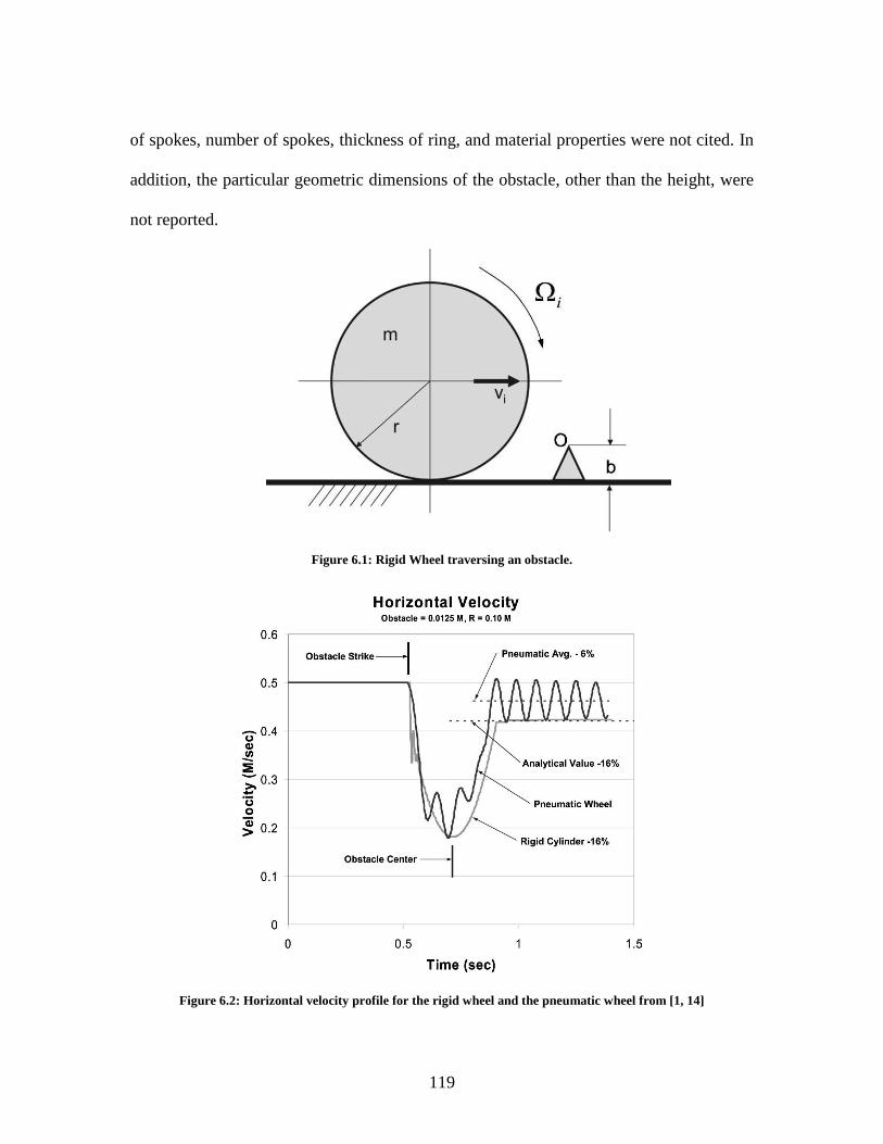
119
of spokes, number of spokes, thickness of ring, and material properties were not cited. In
addition, the particular geometric dimensions of the obstacle, other than the height, were
not reported.
Figure 6.1: Rigid Wheel traversing an obstacle.
Figure 6.2: Horizontal velocity profile for the rigid wheel and the pneumatic wheel from [1, 14]
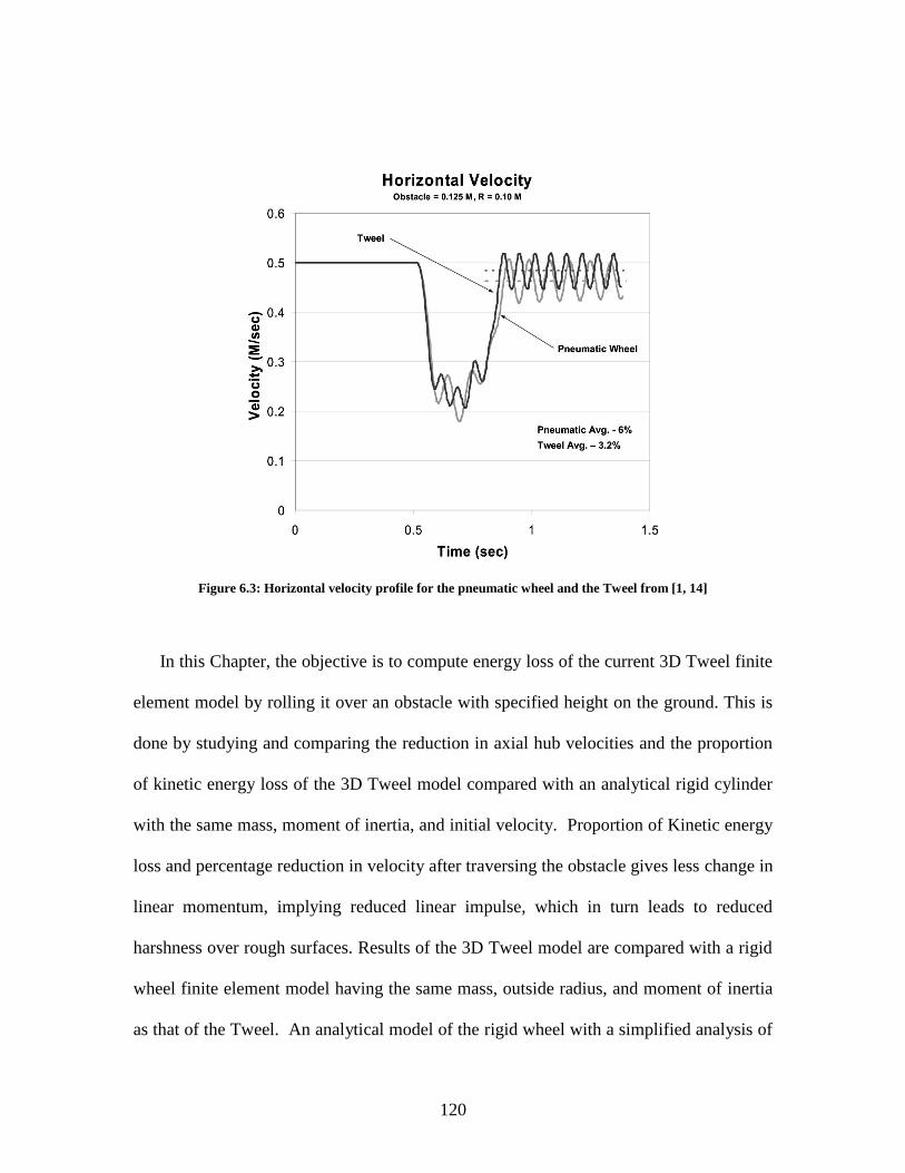
120
Figure 6.3: Horizontal velocity profile for the pneumatic wheel and the Tweel from [1, 14]
In this Chapter, the objective is to compute energy loss of the current 3D Tweel finite
element model by rolling it over an obstacle with specified height on the ground. This is
done by studying and comparing the reduction in axial hub velocities and the proportion
of kinetic energy loss of the 3D Tweel model compared with an analytical rigid cylinder
with the same mass, moment of inertia, and initial velocity. Proportion of Kinetic energy
loss and percentage reduction in velocity after traversing the obstacle gives less change in
linear momentum, implying reduced linear impulse, which in turn leads to reduced
harshness over rough surfaces. Results of the 3D Tweel model are compared with a rigid
wheel finite element model having the same mass, outside radius, and moment of inertia
as that of the Tweel. An analytical model of the rigid wheel with a simplified analysis of

121
the obstacle is also developed and is compared with FEA models of both the Tweel and
rigid wheel.
In order to study the effects of changes in Tweel stiffness on the amount of energy
loss, changes in hyperelastic material models with increase and decrease in shear
modulus described in earlier Chapters is presented. A material study is performed to
compare these parameters for the Tweel model with changing materials for the ring and
the spoke. For this study, rolling resistance is not of interest, thus viscoelastic properties
for the rubber tread are not included in the model.
6.1 Theoretical Speed Reduction and Energy Loss for a Rigid Wheel Traversing an
Obstacle
In theory, the kinematics and kinetics of a rigid wheel rolling over an obstacle is
considered for evaluating the loss of energy and reduction in axial velocity when the
wheel hits and overcomes the obstacle of specified height. The following analysis follows
the discussion in [1] and [18].
Consider a rigid cylinder of mass m, rolling across the ground with a constant
initial velocity Vi. When a rigid wheel of mass „m‟ and radius „R‟ is rolling over an
obstacle of height „b‟, it is assumed that the ground is rough, i.e. no slip takes place, and
no rebound occurs at impact. In other words, the coefficient of restitution is zero which
makes the type of impact to be inelastic. Another important assumption is that the time of
impact is considered to be small so that non-impulsive forces can be neglected. This
conserves the angular momentum of the rigid wheel about point the point of initial

122
impact, denoted pt. O in Figure 6.1. Taking these assumptions into consideration, and
using conservation of angular momentum about the contact point, the speed just after the
initial impact is obtained. Using work energy principles, and conservation of angular
momentum about the second impact when the wheel impacts the ground after pivoting
over the obstacle, an expression can be derived for the final velocity of the rigid wheel
after completely transversing the obstacle (see Appendix).
2
1f i
bV C V
R
where, 21/ (( / ) 1)GC k R , and /G zk I m , Vf is the final velocity after
impact, Vi is the velocity before impact, b is the height of the obstacle and R is the radius
of the wheel. This theoretical value for final velocity will be used to compare with the
values which will be obtained in the numerical simulations.
Given the initial velocity, the
radius of the rigid wheel and the height of the obstacle, the final velocity after impact can
be calculated. Using the expression for final velocity in terms of initial velocity, the
expression for proportion of kinetic energy lost due to an impact of the rigid wheel over
an obstacle is given as (see Appendix)
4
1 1i
E bC
E R
where Ei is the initial kinetic energy and E = Ei – Ef, is the energy loss. The different
parameters used to calculate the proportion of energy lost due to impact and the final
velocity of the rigid wheel after impact is given in the form of a table below.

123
Table 6-1: Parameters for analysis of energy loss rolling over the obstacle
From these set of parameters, the theoretical final velocity for a rigid wheel is be
calculated as 2758.8 mm/s. This results in a percentage relative reduction in axial hub
velocity of 8.04%.
The theoretical kinetic energy of the rigid wheel is a sum of two components. The
first component is the translational kinetic energy due to the axial hub velocity Vi and the
second component is the rotational kinetic energy due to the rotational velocity ω and the
moment of inertia Iz. The analytical equation for the theoretical total initial energy is
2 21 1 +
2 2initial translational rotational i zE E E mV I
With no slip between the wheel and ground, the initial angular speed can be
expressed by the kinematic relation, /iV R . Using the parameters in the setup, the
initial angular velocity is calculated to be 9.891 rad/sec. From the parameters listed
above in Table 6-1, the total initial kinetic energy is Einitial = 12593.7 dN-mm, and the
energy lost due to impact over the obstacle is estimated to be E / Ei = 15.43%. The final
kinetic energy based on the proportion of energy lost is calculated as,
(1 .1543) 10651final initialE E dN mm
Initial axial hub velocity, Vi 3000 mm/sec
Vertical Load 366.5 daN
Outer Radius, R 303.28 mm
Obstacle height, b 22.5 mm
Moment of Inertia, Iz 1.150345 kg-m2
Mass, m 15.4814 kg
Ratio of height of obstacle to the
radius of the rigid wheel, b/R 0.074
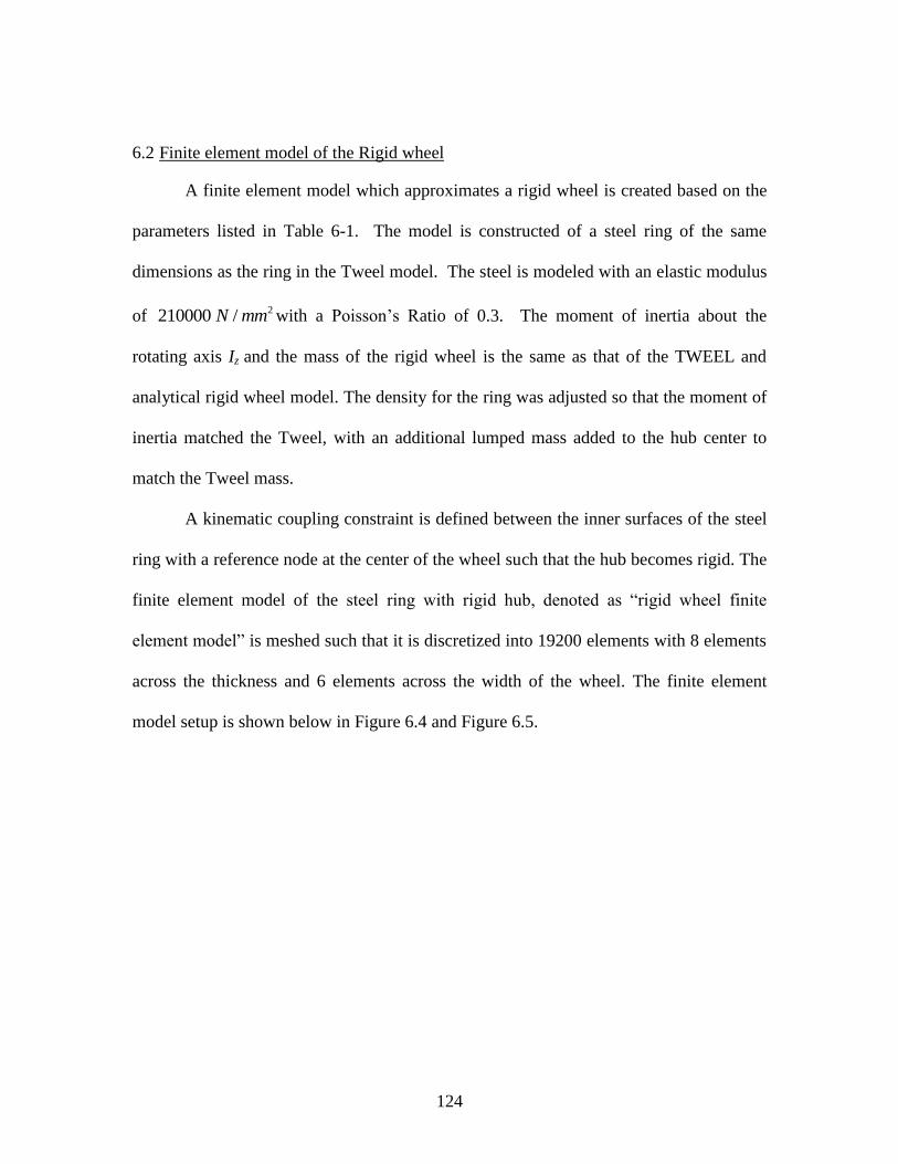
124
6.2 Finite element model of the Rigid wheel
A finite element model which approximates a rigid wheel is created based on the
parameters listed in Table 6-1. The model is constructed of a steel ring of the same
dimensions as the ring in the Tweel model. The steel is modeled with an elastic modulus
of 2210000 /N mm with a Poisson‟s Ratio of 0.3. The moment of inertia about the
rotating axis Iz and the mass of the rigid wheel is the same as that of the TWEEL and
analytical rigid wheel model. The density for the ring was adjusted so that the moment of
inertia matched the Tweel, with an additional lumped mass added to the hub center to
match the Tweel mass.
A kinematic coupling constraint is defined between the inner surfaces of the steel
ring with a reference node at the center of the wheel such that the hub becomes rigid. The
finite element model of the steel ring with rigid hub, denoted as “rigid wheel finite
element model” is meshed such that it is discretized into 19200 elements with 8 elements
across the thickness and 6 elements across the width of the wheel. The finite element
model setup is shown below in Figure 6.4 and Figure 6.5.

125
Figure 6.4: Finite element model of the rigid wheel
Figure 6.5: Enforcement of a kinematic coupling constraint to model rigid hub.
126
This simulation for the rigid wheel modeled a steel ring with rigid hub is
performed in ABAQUS/Explicit. After applying the vertical load, and accelerating up to
a speed of 3000 mm/sec, the wheel model is allowed to roll freely under its own
momentum keeping the vertical load constant. The axial hub velocity time-history for the
rigid model is shown in Figure 6.6. The drop in axial velocity is due to the rolling over
the obstacle. On taking the average of the velocity values between t=1.27 and t=1.4, the
final velocity after traversing the obstacle is calculated to be 2754.323 mm/s. When
compared with the analytical rigid wheel final velocity of 2758.8 mm/s, the difference is
only 0.16%, showing good agreement.
The kinetic energy of the finite element model of the rigid wheel is shown in
Figure 6.7. On taking the average of the kinetic energy values between t=1.27 and t=1.4,
the value is calculated to be 10661 dN-mm. When compared with the analytical rigid
wheel model with value of 10651dN-mm, the difference in final kinetic energy is
calculated as 0.09%.

127
Figure 6.6: Comparison of the axial hub velocity of the finite element rigid wheel model based on a steel ring
with the analytical model.
Figure 6.7: Comparison of the kinetic energy of the finite element rigid wheel model with the analytical model.
1 1.05 1.1 1.15 1.2 1.25 1.3 1.35 1.41400
1600
1800
2000
2200
2400
2600
2800
3000
3200
Time (sec)
Axia
l H
ub V
elo
city (
mm
/s)
Axial Hub velocity (Rigid Wheel)
Axial Hub velocity (Analytical)
Axial Hub velocity average(Rigid Wheel)
1 1.05 1.1 1.15 1.2 1.25 1.3 1.35 1.43000
4000
5000
6000
7000
8000
9000
10000
11000
12000
13000
Time (sec)
Kin
etic e
nerg
y (
dN
.mm
)
Kinetic energy (Rigid Wheel)
Kinetic energy (Analytical)
Kinetic energy average(Rigid Wheel)

128
The conservation of energy states that time rate of change of kinetic energy and
internal energy of a body of material is equal to the sum of the rate of work done by the
surface and body forces [19]. This can be expressed as,
( )K U WF
dE E E
dt
where EK = kinetic energy, and EU = internal energy, and EWF = external work. The total
internal energy can be split into an internal energy from for the material and viscous
dissipation energy, such that EU = EI + EV. The rate of change in external work can be
defined in terms of the rate of change of work done by external forces, and the rate of
energy dissipated by contact frictional forces between the contact surfaces, such that EWF
= EW – EF. An energy balance for the entire model can then be obtained by integrating
the above equation:
constantTotal K I V F WE E E E E E
From Figure 6.8, it is seen that the kinetic energy and external work of the rigid
wheel finite element model increases during the acceleration step between 0 and 1.1 sec.
After traversing the obstacle, the Kinetic Energy is reduced by 15%. To maintain a
constant zero total energy as defined in the above equation, the loss in kinetic energy is
accounted for by a corresponding increase in internal energy and to a lesser degree,
frictional energy dissipation ( minus work due to friction). This increase in the internal
energy can be accounted for by the constrained elastic vibrations developed in the steel
ring after impacting the obstacle and ground. Also, when the wheel impacts the obstacle,
the energy due to frictional dissipation also starts to increase.
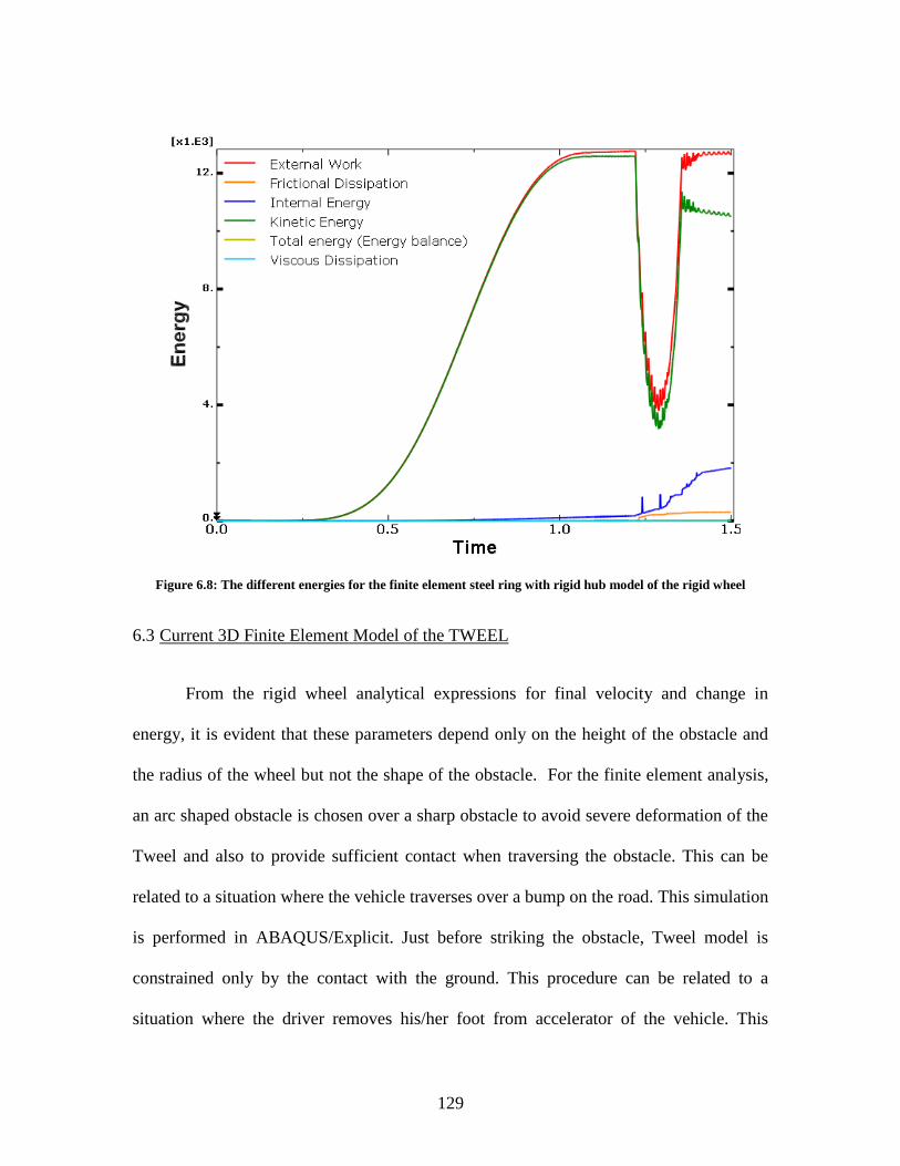
129
Figure 6.8: The different energies for the finite element steel ring with rigid hub model of the rigid wheel
6.3 Current 3D Finite Element Model of the TWEEL
From the rigid wheel analytical expressions for final velocity and change in
energy, it is evident that these parameters depend only on the height of the obstacle and
the radius of the wheel but not the shape of the obstacle. For the finite element analysis,
an arc shaped obstacle is chosen over a sharp obstacle to avoid severe deformation of the
Tweel and also to provide sufficient contact when traversing the obstacle. This can be
related to a situation where the vehicle traverses over a bump on the road. This simulation
is performed in ABAQUS/Explicit. Just before striking the obstacle, Tweel model is
constrained only by the contact with the ground. This procedure can be related to a
situation where the driver removes his/her foot from accelerator of the vehicle. This

130
makes the vehicle to cross the obstacle with the momentum gained from the previous
step. The scenario created for a rigid wheel is replicated for the Tweel. The procedure
and the boundary conditions used in this problem have been explained in Chapter Two.
To set up the model, one should determine the distance travelled by the Tweel model
during each analysis step. This distance can be calculated using fundamental equations of
kinematics. Starting from rest during the constant acceleration during Step 1, the distance
traveled is determined from
1( )
2step final initial stepS V V t
In the following, all dimensions are expressed in millimeters (mm). The velocity
is defined in millimeters per second (mm/s).
In Step 1, the Tweel is accelerated to a final velocity of 3000 mm/s over a period
of 1 second. The distance travelled in the first step is calculated to be 1500 mm. In Step
2, the Tweel is maintained at a constant velocity of 3000 mm/s (10.8 km/hr) for 0.1
seconds. The distance travelled in this step is 300 mm. In Step 3, the Tweel model is now
free to roll with the momentum gained from the previous step for a time period of 0.4
seconds. Since the deceleration of the Tweel is not known a priori when it traverses the
obstacle, the analytically rigid ground is created such that there is sufficient distance for
the Tweel to travel. A safe total of 5000 mm is estimated to be the length of the ground.
This setup is shown in Figure 6.9, Figure 6.10 and Figure 6.11.

131
Figure 6.9: Analysis set up for Tweel rolling over rigid obstacle of height b = 0.074 R.
Figure 6.10: Analysis set up of the 3D Tweel finite element model rolling over an obstacle

132
Figure 6.11: XY view of the Finite Element model setup
6.4 Results during obstacle impact
The Reference Tweel model considered for this analysis is a three dimensional
Tweel with Marlow properties for both the ring and the spokes.
Figure 6.12 and Figure 6.13 show the Tweel model during initial impact with the
obstacle.
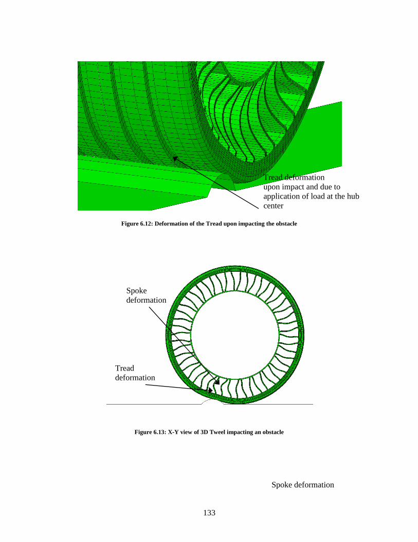
133
Figure 6.12: Deformation of the Tread upon impacting the obstacle
Figure 6.13: X-Y view of 3D Tweel impacting an obstacle
Tread deformation
upon impact and due to
application of load at the hub
center
Tread
deformation
Spoke
deformation
Spoke deformation
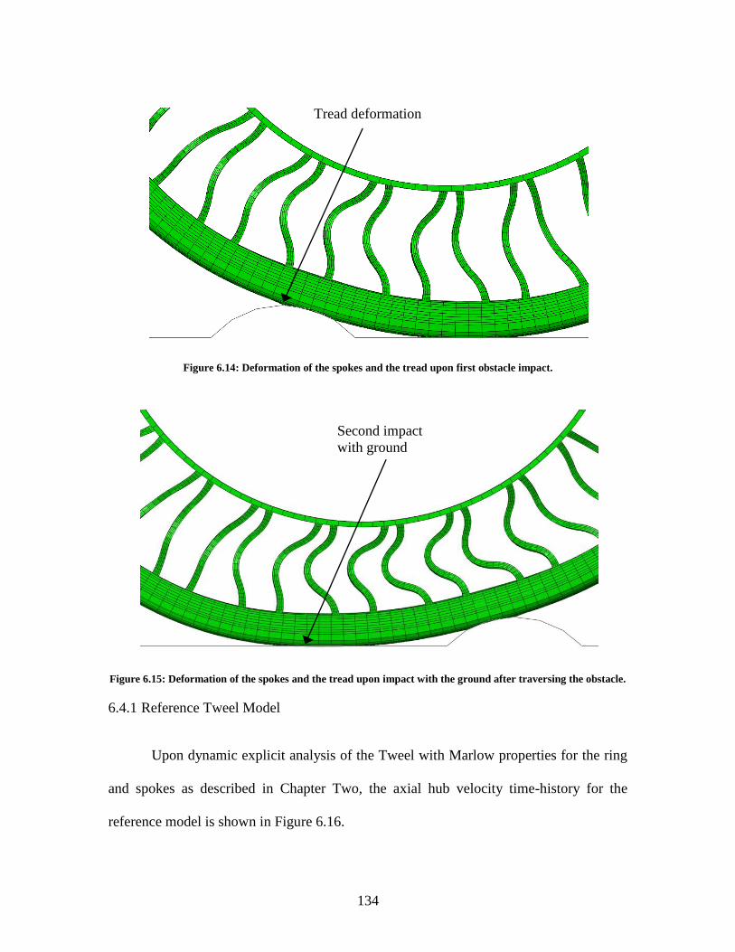
134
Figure 6.14: Deformation of the spokes and the tread upon first obstacle impact.
Figure 6.15: Deformation of the spokes and the tread upon impact with the ground after traversing the obstacle.
6.4.1 Reference Tweel Model
Upon dynamic explicit analysis of the Tweel with Marlow properties for the ring
and spokes as described in Chapter Two, the axial hub velocity time-history for the
reference model is shown in Figure 6.16.
Tread deformation
Second impact
with ground

135
Figure 6.16: The axial hub velocity of the TWEEL in comparison with the rigid wheel.
From time 1 < t < 1.1, the Tweel is maintained at a constant velocity of 3000
mm/sec. From the next increment after t=1.1, as explained earlier, no kinematic
constraints other than contact with the ground surface are enforced. After initial impact,
the Tweel rolls up over the obstacle with height b = 22.5 mm, and the axial velocity drops
to 1797 mm/s at t=1.172 sec. This drop is recorded at the maximum obstacle height.
Once the Tweel rolls over from the obstacle, the velocity again increases to a peak value
of 3068 mm/s at t=1.239. This is the point where the Tweel impacts the flat ground after
traversing the obstacle. From 1.239 < t < 1.5, the vibration seen in the Figure is due to the
hyperelastic response of the Tweel when it impacts the ground after traversing the
obstacle. On taking the average of the velocity values between 1.3 < t < 1.5, the average
velocity value is calculated to be 2962 mm/sec. This shows that the reduction in the axial
1 1.05 1.1 1.15 1.2 1.25 1.3 1.35 1.4 1.45 1.51400
1600
1800
2000
2200
2400
2600
2800
3000
3200
Time (sec)
Axia
l H
ub V
elo
city (
mm
/s)
Axial Hub velocity (Rigid Wheel)
Axial Hub velocity (TWEEL-Marlow)
Axial Hub velocity average(Rigid Wheel)
Axial Hub velocity average(TWEEL-Marlow)
Axial hub velocity (Analytical)

136
hub velocity is 1.265%. This is calculated by taking the initial hub velocity of 3000 mm/s
and the final velocity to be the average value that was calculated, i.e.
3000 2962 .01265
3000
i f
i i
V VV
V V
The Tweel hub velocity reduction of 1.265% is significantly lower than the
approximately 8% velocity reduction found in the rigid wheel models. This result is
consistent with the trend in values reported in [1]. As discussed earlier, a reduction in
axial velocity corresponds to a reduction in linear momentum, which implies an increase
in linear impulse, and harshness.
Figure 6.17: Kinetic energy of the TWEEL in comparison with the Rigid wheel.
Figure 6.17 shows the kinetic energy (KE) profile for the reference model. We
observe that prior to impact, the average kinetic energy for the Tweel model is 12870.95
dN-mm, which is higher than the initial kinetic energy of 12593.7 dN-mm predicted by
the rigid analytical model. The increase in the initial KE for the Tweel model can be
1 1.05 1.1 1.15 1.2 1.25 1.3 1.35 1.4 1.45 1.53000
4000
5000
6000
7000
8000
9000
10000
11000
12000
13000
Time (sec)
Kin
etic e
nerg
y (
dN
.mm
)
Kinetic energy (Rigid Wheel)
Kinetic energy (TWEEL-Marlow)
Kinetic energy average(Rigid Wheel)
Kinetic energy average(TWEEL-Marlow)
Kinetic energy (Analytical)

137
explained due to the local motion of the hyperelastic spokes and ring during rolling and
also due to buckling and snapping back of spokes when entering and exiting the contact
region, which is not accounted for in the analytical rigid model.
After impacting the obstacle, the average kinetic energy of the Tweel is 12569.1
dN-mm. The final kinetic energy in the Tweel model includes all sources of motion,
including vertical motion due to the hyperelastic bouncing effect and internal vibrations
after traversing the obstacle and impacting the rigid ground.
The velocity and the kinetic energy values for the analytical model of the rigid
wheel, the finite element model of the rigid wheel modeled as a steel ring with rigid hub
and the Tweel are summarized in Table 6-2.
Table 6-2: Summary of the velocity and K.E values of the analytical rigid wheel, finite element rigid wheel and
the Tweel
Initial
velocity
(mm/s)
Final
velocity
(mm/s)
Reduction
in velocity
Initial
K.E
(dN-mm)
Final
K.E
(dN-mm)
Reduction
in K.E
Analytical
Rigid
Wheel
3000 2758.8 8.04% 12593.7 10651 15.4%
Finite
Element
Rigid
Wheel
3000 2754.32 8.2% 12570 10661 15.2%
Tweel 3000 2962 1.265% 12871 12569 2.34%
For reference, the vertical component of velocity and angular speed of the Tweel
hub during the impact event from 1 sec to 1.5 sec is shown in Figure 6.18 and Figure
6.19.

138
Figure 6.18: Vertical hub velocity profile of the Reference Marlow model
Figure 6.19: Rotational velocity profile of the Reference Marlow model.
Comparing the average initial kinetic energy to the average final kinetic energy,
the energy loss is 2.3457%. From the results in Figure 6.16 and Figure 6.17, it can be
concluded that the Tweel loses significantly less energy than the analytical rigid wheel
1 1.05 1.1 1.15 1.2 1.25 1.3 1.35 1.4 1.45 1.5-800
-600
-400
-200
0
200
400
600
800
1000
Time (sec)
Ve
rtic
al H
ub
Ve
locity (
mm
/s)
Vertical Hub velocity profile (Reference)
1 1.05 1.1 1.15 1.2 1.25 1.3 1.35 1.4 1.45 1.55
6
7
8
9
10
11
Time (sec)
Ro
tatio
na
l Ve
locity
(ra
dia
ns/s
ec)
Rotational Velocity profile (Reference)

139
and steel ring with rigid hub finite element rigid wheel when traversing the obstacle. The
reduction in velocities and the proportion of energy lost for different material models are
compared in the following sections of this chapter.
6.4.2 Shear modulus of the Mooney Rivlin model for the ring remains unchanged
From Figure 6.20, the reduction in velocity for the Tweel model with a Mooney
Rivlin unchanged model for the ring is 1.22% corresponding to an average final velocity
of 2963.26 mm/s. Recall that the Tweel model with Marlow properties for the ring
recorded a reduction in average velocity of 1.265% (2962 mm/s).
Figure 6.20: Axial hub velocity profiles of the Tweel with Marlow properties (1.265%) and an unchanged
Mooney Rivlin material model for the ring (1.22%)
In Figure 6.21 the average initial kinetic energy for the unchanged Mooney Rivlin
model for the ring is 12890.59064 daN - mm. The average kinetic energy for the same
1 1.05 1.1 1.15 1.2 1.25 1.3 1.35 1.4 1.45 1.51600
1800
2000
2200
2400
2600
2800
3000
3200
Time (sec)
Axia
l H
ub V
elo
city (
mm
/s)
Reference
MooneyRivlin 0 unchanged
Average Velocity (Reference)
Average Velocity (MooneyRivlin 0 unchanged)
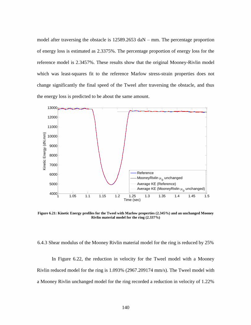
140
model after traversing the obstacle is 12589.2653 daN – mm. The percentage proportion
of energy loss is estimated as 2.3375%. The percentage proportion of energy loss for the
reference model is 2.3457%. These results show that the original Mooney-Rivlin model
which was least-squares fit to the reference Marlow stress-strain properties does not
change significantly the final speed of the Tweel after traversing the obstacle, and thus
the energy loss is predicted to be about the same amount.
Figure 6.21: Kinetic Energy profiles for the Tweel with Marlow properties (2.345%) and an unchanged Mooney
Rivlin material model for the ring (2.337%)
6.4.3 Shear modulus of the Mooney Rivlin material model for the ring is reduced by 25%
In Figure 6.22, the reduction in velocity for the Tweel model with a Mooney
Rivlin reduced model for the ring is 1.093% (2967.209174 mm/s). The Tweel model with
a Mooney Rivlin unchanged model for the ring recorded a reduction in velocity of 1.22%
1 1.05 1.1 1.15 1.2 1.25 1.3 1.35 1.4 1.45 1.54000
5000
6000
7000
8000
9000
10000
11000
12000
13000
Time (sec)
Kin
etic E
nerg
y (
dN
.mm
)
Reference
MooneyRivlin 0 unchanged
Average KE (Reference)
Average KE (MooneyRivlin 0 unchanged)
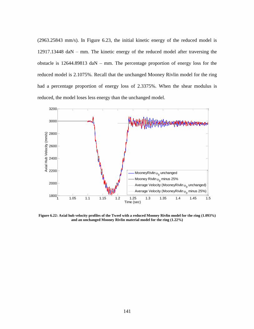
141
(2963.25843 mm/s). In Figure 6.23, the initial kinetic energy of the reduced model is
12917.13448 daN – mm. The kinetic energy of the reduced model after traversing the
obstacle is 12644.89813 daN – mm. The percentage proportion of energy loss for the
reduced model is 2.1075%. Recall that the unchanged Mooney Rivlin model for the ring
had a percentage proportion of energy loss of 2.3375%. When the shear modulus is
reduced, the model loses less energy than the unchanged model.
Figure 6.22: Axial hub velocity profiles of the Tweel with a reduced Mooney Rivlin model for the ring (1.093%)
and an unchanged Mooney Rivlin material model for the ring (1.22%)
1 1.05 1.1 1.15 1.2 1.25 1.3 1.35 1.4 1.45 1.51800
2000
2200
2400
2600
2800
3000
3200
Time (sec)
Axia
l H
ub
Ve
locity (
mm
/s)
MooneyRivlin 0 unchanged
Mooney Rivlin 0 minus 25%
Average Velocity (MooneyRivlin 0 unchanged)
Average Velocity (MooneyRivlin 0 minus 25%)

142
Figure 6.23: Kinetic Energy profiles for the Tweel with a reduced Mooney Rivlin material model (2.1075%) and
an unchanged Mooney Rivlin material model for the ring (2.3375%)
6.4.4 Shear modulus of the Mooney Rivlin model for the ring is increased by 25%
In Figure 6.24, the reduction in velocity for the Tweel model with a Mooney
Rivlin increased model for the ring is 1.368% (2958.930537 mm/s). The Tweel model
with a Mooney Rivlin unchanged model for the ring recorded a reduction in velocity of
1.22% (2963.25843 mm/s). In Figure 6.25, the initial kinetic energy of the Mooney
Rivlin model with an increased shear modulus is 12870.36355 daN – mm. The final
kinetic energy after traversing the obstacle is 12551.00858 daN – mm. The percentage
proportion of energy lost for the Mooney Rivlin model with increased shear modulus is
2.4813%. Recall that the percentage proportion of energy lost for a Mooney Rivlin model
1 1.05 1.1 1.15 1.2 1.25 1.3 1.35 1.4 1.45 1.54000
5000
6000
7000
8000
9000
10000
11000
12000
13000
Time (sec)
Kin
etic E
ne
rgy (
dN
.mm
)
Mooney Rivlin 0 unchanged
Mooney Rivlin 0 minus 25%
Average KE (MooneyRivlin 0 unchanged)
Average KE (MooneyRivlin 0 minus 25%)
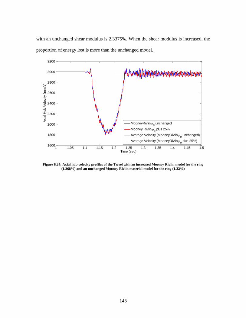
143
with an unchanged shear modulus is 2.3375%. When the shear modulus is increased, the
proportion of energy lost is more than the unchanged model.
Figure 6.24: Axial hub velocity profiles of the Tweel with an increased Mooney Rivlin model for the ring
(1.368%) and an unchanged Mooney Rivlin material model for the ring (1.22%)
1 1.05 1.1 1.15 1.2 1.25 1.3 1.35 1.4 1.45 1.51600
1800
2000
2200
2400
2600
2800
3000
3200
Time (sec)
Axia
l H
ub
Ve
locity (
mm
/s)
MooneyRivlin 0 unchanged
Mooney Rivlin 0 plus 25%
Average Velocity (MooneyRivlin 0 unchanged)
Average Velocity (MooneyRivlin 0 plus 25%)

144
Figure 6.25: Kinetic Energy profiles for the Tweel with a reduced Mooney Rivlin material model (2.4813%) and
an unchanged Mooney Rivlin material model for the ring (2.3375%)
6.4.5 Shear modulus of the Neo Hookean material model for the ring remains unchanged
From Figure 6.26, the reduction in velocity for the Tweel model with a Neo
Hookean unchanged model for the ring is 1.314% (2960.560868 mm/s). The Tweel
model with Marlow properties for the ring recorded a reduction in velocity of 1.265%
(2962.052025 mm/s). In Figure 6.27, the initial kinetic energy of the unchanged Neo
Hookean model for the ring is 12941.90394 daN – mm. The final kinetic energy after
traversing the obstacle is 12612.87425 daN – mm. The percentage proportion of energy
loss is calculated to be 2.5423%. Recall that the percentage proportion of energy lost for
the reference Marlow model is 2.3457%. From these results show that the Tweel with an
unchanged Neo Hookean model for the ring loses more energy upon impact than the
Marlow model.
1 1.05 1.1 1.15 1.2 1.25 1.3 1.35 1.4 1.45 1.54000
5000
6000
7000
8000
9000
10000
11000
12000
13000
Time (sec)
Kin
etic E
ne
rgy (
dN
.mm
)
Mooney Rivlin 0 unchanged
Mooney Rivlin 0 plus 25%
Average KE (MooneyRivlin 0 unchanged)
Average KE (MooneyRivlin 0 plus 25%)
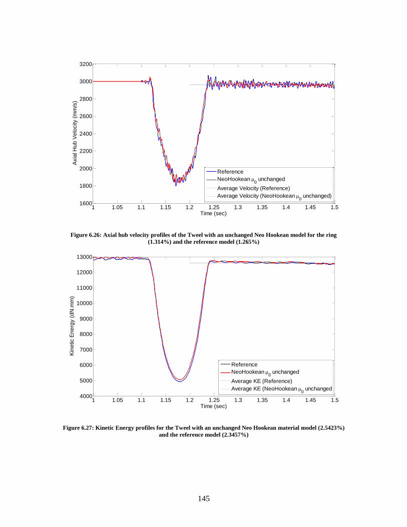
145
Figure 6.26: Axial hub velocity profiles of the Tweel with an unchanged Neo Hookean model for the ring
(1.314%) and the reference model (1.265%)
Figure 6.27: Kinetic Energy profiles for the Tweel with an unchanged Neo Hookean material model (2.5423%)
and the reference model (2.3457%)
1 1.05 1.1 1.15 1.2 1.25 1.3 1.35 1.4 1.45 1.51600
1800
2000
2200
2400
2600
2800
3000
3200
Time (sec)
Axia
l H
ub
Ve
locity (
mm
/s)
Reference
NeoHookean 0 unchanged
Average Velocity (Reference)
Average Velocity (NeoHookean 0 unchanged)
1 1.05 1.1 1.15 1.2 1.25 1.3 1.35 1.4 1.45 1.54000
5000
6000
7000
8000
9000
10000
11000
12000
13000
Time (sec)
Kin
etic E
ne
rgy (
dN
.mm
)
Reference
NeoHookean 0 unchanged
Average KE (Reference)
Average KE (NeoHookean 0 unchanged

146
6.4.6 Shear modulus of the Neo Hookean material model for the ring is reduced by 25%
In Figure 6.28, the reduction in velocity for the Tweel model with a Neo Hookean
unchanged model for the ring is 1.314% (2960.560868 mm/s). The Tweel model with a
Neo Hookean reduced model recorded a reduction in velocity of 1.87% (2943.875393
mm/s). In Figure 6.29, the initial kinetic energy of the Neo Hookean model with a
reduced shear modulus is 12962.68621 daN – mm. The final kinetic energy of the model
after traversing the obstacle is 12531.30485 daN – mm. The percentage proportion of
energy lost upon impact is 3.3278%. Recall that the percentage proportion of energy lost
upon impact for the unchanged Neo Hookean model is 2.5423%. Hence, from these
results, it can be said that the Neo Hookean reduced model for the ring loses more energy
than the Neo Hookean unchanged model.
Figure 6.28: Axial hub velocity profiles of the Tweel with an unchanged Neo Hookean model for the ring
(1.314%) and a reduced Neo Hookean model (1.87%)
1 1.05 1.1 1.15 1.2 1.25 1.3 1.35 1.4 1.45 1.51800
2000
2200
2400
2600
2800
3000
3200
Time (sec)
Axia
l H
ub
Ve
locity (
mm
/s)
NeoHookean 0 unchanged
NeoHookean 0 minus 25%
Average Velocity (NeoHookean 0 unchanged)
Average Velocity (NeoHookean 0 minus 25%)

147
Figure 6.29: Kinetic Energy profiles for the Tweel with an unchanged Neo Hookean material model (2.5423%)
and a reduced Neo Hookean model (3.3278%)
6.4.7 Shear modulus of the Neo Hookean model for the ring is increased by 25%
In Figure 6.30, the reduction in velocity for the Tweel model with a Neo Hookean
unchanged model for the ring is 1.314% (2960.560868 mm/s). The Tweel model with a
Neo Hookean increased model recorded a reduction in velocity of 1.139% (2965.820165
mm/s). From Figure 6.31, the initial kinetic energy of the Neo Hookean with increased
shear modulus is 12923.47783 daN – mm. The final kinetic energy of the model after
traversing the obstacle is 12633.3694 daN – mm. The percentage proportion of energy
lost is 2.2448%. On comparing with the unchanged Neo Hookean model, the increased
model loses less energy.
1 1.05 1.1 1.15 1.2 1.25 1.3 1.35 1.4 1.45 1.55000
6000
7000
8000
9000
10000
11000
12000
13000
14000
Time (sec)
Kin
etic E
ne
rgy (
dN
.mm
)
NeoHookean 0 unchanged
NeoHookean 0 minus 25%
Average KE (NeoHookean 0 unchanged)
Average KE (NeoHookean 0 minus 25%)
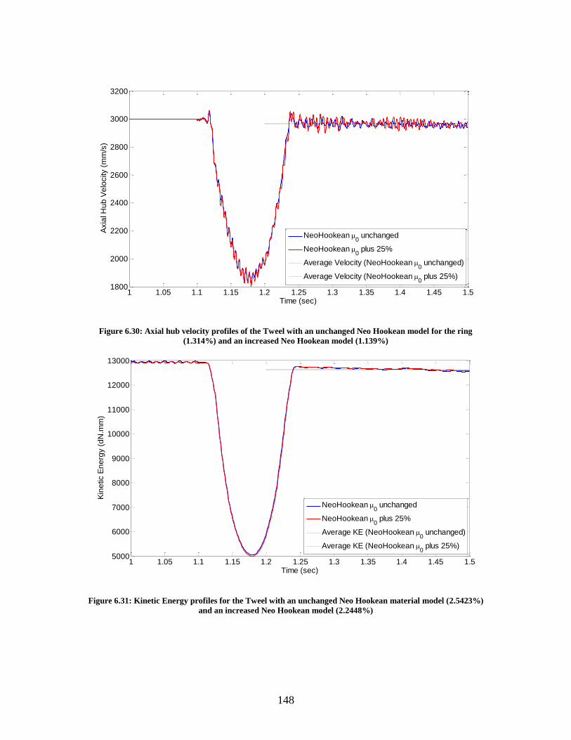
148
Figure 6.30: Axial hub velocity profiles of the Tweel with an unchanged Neo Hookean model for the ring
(1.314%) and an increased Neo Hookean model (1.139%)
Figure 6.31: Kinetic Energy profiles for the Tweel with an unchanged Neo Hookean material model (2.5423%)
and an increased Neo Hookean model (2.2448%)
1 1.05 1.1 1.15 1.2 1.25 1.3 1.35 1.4 1.45 1.51800
2000
2200
2400
2600
2800
3000
3200
Time (sec)
Axia
l H
ub
Ve
locity (
mm
/s)
NeoHookean 0 unchanged
NeoHookean 0 plus 25%
Average Velocity (NeoHookean 0 unchanged)
Average Velocity (NeoHookean 0 plus 25%)
1 1.05 1.1 1.15 1.2 1.25 1.3 1.35 1.4 1.45 1.55000
6000
7000
8000
9000
10000
11000
12000
13000
Time (sec)
Kin
etic E
ne
rgy (
dN
.mm
)
NeoHookean 0 unchanged
NeoHookean 0 plus 25%
Average KE (NeoHookean 0 unchanged)
Average KE (NeoHookean 0 plus 25%)

149
6.4.8 Shear modulus of the Mooney Rivlin model for the spokes remains unchanged
In Figure 6.32, the reduction in velocity for the Tweel model with a Mooney
Rivlin unchanged model for the spoke is 1.32% (2960.30396 mm/s). The Tweel model
with Marlow properties recorded a reduction in velocity of 1.265% (2962.052025 mm/s).
Figure 6.32: Axial hub velocity profile of the Tweel with Mooney Rivlin unchanged model on the spokes (1.32%)
and with Marlow properties (1.265%)
From Figure 6.33, the initial kinetic energy for the unchanged Mooney Rivlin
model for the spokes is 12899.21232 daN – mm. The final kinetic energy after traversing
the obstacle is 12573.40336 daN – mm. The percentage proportion of energy loss is
2.5258%. On comparing with the reference Marlow model, the Mooney Rivlin
unchanged model for the spokes loses more energy.
1 1.05 1.1 1.15 1.2 1.25 1.3 1.35 1.4 1.45 1.51600
1800
2000
2200
2400
2600
2800
3000
3200
Time (sec)
Axia
l H
ub
Ve
locity (
mm
/s)
Reference
MooneyRivlin 0 unchanged
Average Velocity (Reference)
Average Velocity (MooneyRivlin 0 unchanged)

150
Figure 6.33: Kinetic energy profiles for the Tweel with Mooney Rivlin for the spokes (2.5258%) and with
Marlow properties (2.3457%)
6.4.9 Shear modulus of the Mooney Rivlin material for the spokes is reduced by 25%
In Figure 6.34, the reduction in velocity for the Tweel model with a Mooney
Rivlin unchanged model for the spoke is 1.32% (2960.30396 mm/s). The Tweel model
with a Mooney Rivlin reduced model for the spokes recorded a reduction in velocity of
1.034% (2968.964607 mm/s). In Figure 6.35, the initial kinetic energy of the Mooney
Rivlin model with reduced shear modulus is 12940.29507 daN – mm. The final kinetic
energy after traversing the obstacle is 12686.73396 daN – mm. The percentage
proportion of energy lost is 1.9594%. On comparing with the unchanged Mooney Rivlin
model, the reduced Mooney Rivlin model for the spokes loses less energy.
1 1.05 1.1 1.15 1.2 1.25 1.3 1.35 1.4 1.45 1.54000
5000
6000
7000
8000
9000
10000
11000
12000
13000
Time (sec)
Kin
etic E
ne
rgy (
dN
.mm
)
Reference
MooneyRivlin 0 unchanged
Average KE (Reference)
Average KE (MooneyRivlin 0 unchanged

151
Figure 6.34: Axial hub velocity profile for the Tweel with a Mooney Rivlin unchanged model (1.32%) and a
Mooney Rivlin reduced model (1.034%)
Figure 6.35: Kinetic energy profile for the Tweel with a Mooney Rivlin unchanged model (2.5258%) and a
Mooney Rivlin reduced model (1.9594%)
1 1.05 1.1 1.15 1.2 1.25 1.3 1.35 1.4 1.45 1.51800
2000
2200
2400
2600
2800
3000
3200
Time (sec)
Axia
l H
ub
Ve
locity (
mm
/s)
MooneyRivlin 0 unchanged
MooneyRivlin 0 minus 25%
Average Velocity (MooneyRivlin 0 unchanged)
Average Velocity (MooneyRivlin 0 minus 25%)
1 1.05 1.1 1.15 1.2 1.25 1.3 1.35 1.4 1.45 1.54000
5000
6000
7000
8000
9000
10000
11000
12000
13000
14000
Time (sec)
Kin
etic E
ne
rgy (
dN
.mm
)
MooneyRivlin 0 unchanged
MooneyRivlin 0 minus 25%
Average KE (MooneyRivlin 0 unchanged)
Average KE (MooneyRivlin 0 minus 25%)
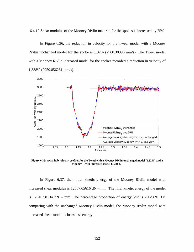
152
6.4.10 Shear modulus of the Mooney Rivlin material for the spokes is increased by 25%
In Figure 6.36, the reduction in velocity for the Tweel model with a Mooney
Rivlin unchanged model for the spoke is 1.32% (2960.30396 mm/s). The Tweel model
with a Mooney Rivlin increased model for the spokes recorded a reduction in velocity of
1.338% (2959.856281 mm/s).
Figure 6.36: Axial hub velocity profiles for the Tweel with a Mooney Rivlin unchanged model (1.32%) and a
Mooney Rivlin increased model (1.338%)
In Figure 6.37, the initial kinetic energy of the Mooney Rivlin model with
increased shear modulus is 12867.65616 dN – mm. The final kinetic energy of the model
is 12548.58134 dN – mm. The percentage proportion of energy lost is 2.4796%. On
comparing with the unchanged Mooney Rivlin model, the Mooney Rivlin model with
increased shear modulus loses less energy.
1 1.05 1.1 1.15 1.2 1.25 1.3 1.35 1.4 1.45 1.51600
1800
2000
2200
2400
2600
2800
3000
3200
Time (sec)
Axia
l H
ub
Ve
locity (
mm
/s)
MooneyRivlin 0 unchanged
MooneyRivlin 0 plus 25%
Average Velocity (MooneyRivlin 0 unchanged)
Average Velocity (MooneyRivlin 0 plus 25%)

153
Figure 6.37: Kinetic energy profiles for the Tweel with a Mooney Rivlin unchanged model (2.5258%) and a
Mooney Rivlin increased model (2.4796%) for the spokes
6.4.11 Shear modulus of the Neo Hookean material for the spokes remains unchanged
In Figure 6.38, the reduction in velocity for the Tweel model with a Neo Hookean
unchanged model for the spoke is 1.28% (2961.582087 mm/s). The Tweel model with
Marlow properties recorded a reduction in velocity of 1.265% (2959.856281 mm/s). In
Figure 6.39, the initial kinetic energy of the unchanged Neo Hookean model is
12983.75172 daN – mm. The final kinetic energy after traversing the obstacle is
12678.47836 daN – mm. The percentage proportion of energy loss is 2.3511%. On
comparing with the reference Marlow model, the unchanged Neo Hookean model loses
slightly more energy.
1 1.05 1.1 1.15 1.2 1.25 1.3 1.35 1.4 1.45 1.54000
5000
6000
7000
8000
9000
10000
11000
12000
13000
Time (sec)
Kin
etic E
ne
rgy (
dN
.mm
)
MooneyRivlin 0 unchanged
MooneyRivlin 0 plus 25%
Average KE (MooneyRivlin 0 unchanged)
Average KE (MooneyRivlin 0 plus 25%)
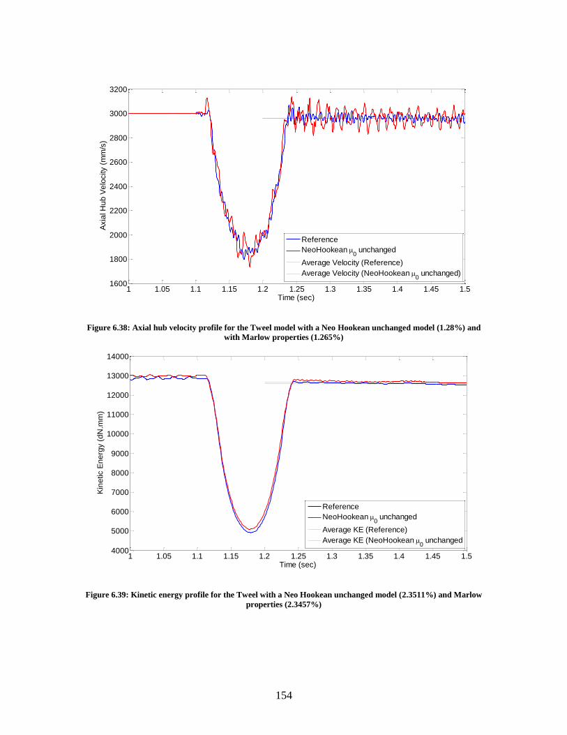
154
Figure 6.38: Axial hub velocity profile for the Tweel model with a Neo Hookean unchanged model (1.28%) and
with Marlow properties (1.265%)
Figure 6.39: Kinetic energy profile for the Tweel with a Neo Hookean unchanged model (2.3511%) and Marlow
properties (2.3457%)
1 1.05 1.1 1.15 1.2 1.25 1.3 1.35 1.4 1.45 1.51600
1800
2000
2200
2400
2600
2800
3000
3200
Time (sec)
Axia
l H
ub
Ve
locity (
mm
/s)
Reference
NeoHookean 0 unchanged
Average Velocity (Reference)
Average Velocity (NeoHookean 0 unchanged)
1 1.05 1.1 1.15 1.2 1.25 1.3 1.35 1.4 1.45 1.54000
5000
6000
7000
8000
9000
10000
11000
12000
13000
14000
Time (sec)
Kin
etic E
ne
rgy (
dN
.mm
)
Reference
NeoHookean 0 unchanged
Average KE (Reference)
Average KE (NeoHookean 0 unchanged
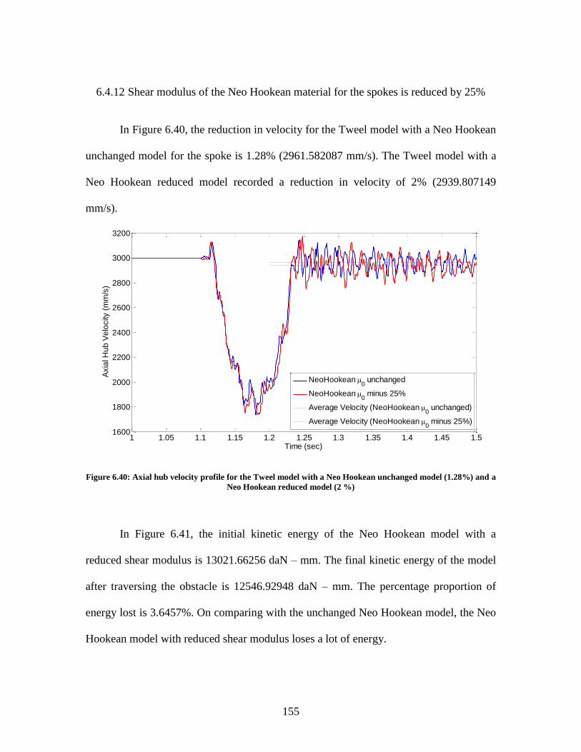
155
6.4.12 Shear modulus of the Neo Hookean material for the spokes is reduced by 25%
In Figure 6.40, the reduction in velocity for the Tweel model with a Neo Hookean
unchanged model for the spoke is 1.28% (2961.582087 mm/s). The Tweel model with a
Neo Hookean reduced model recorded a reduction in velocity of 2% (2939.807149
mm/s).
Figure 6.40: Axial hub velocity profile for the Tweel model with a Neo Hookean unchanged model (1.28%) and a
Neo Hookean reduced model (2 %)
In Figure 6.41, the initial kinetic energy of the Neo Hookean model with a
reduced shear modulus is 13021.66256 daN – mm. The final kinetic energy of the model
after traversing the obstacle is 12546.92948 daN – mm. The percentage proportion of
energy lost is 3.6457%. On comparing with the unchanged Neo Hookean model, the Neo
Hookean model with reduced shear modulus loses a lot of energy.
1 1.05 1.1 1.15 1.2 1.25 1.3 1.35 1.4 1.45 1.51600
1800
2000
2200
2400
2600
2800
3000
3200
Time (sec)
Axia
l H
ub
Ve
locity (
mm
/s)
NeoHookean 0 unchanged
NeoHookean 0 minus 25%
Average Velocity (NeoHookean 0 unchanged)
Average Velocity (NeoHookean 0 minus 25%)
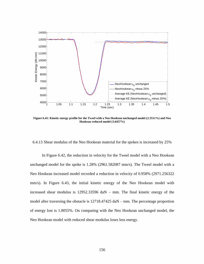
156
Figure 6.41: Kinetic energy profile for the Tweel with a Neo Hookean unchanged model (2.3511%) and Neo
Hookean reduced model (3.6457%)
6.4.13 Shear modulus of the Neo Hookean material for the spokes is increased by 25%
In Figure 6.42, the reduction in velocity for the Tweel model with a Neo Hookean
unchanged model for the spoke is 1.28% (2961.582087 mm/s). The Tweel model with a
Neo Hookean increased model recorded a reduction in velocity of 0.958% (2971.256322
mm/s). In Figure 6.43, the initial kinetic energy of the Neo Hookean model with
increased shear modulus is 12952.33596 daN – mm. The final kinetic energy of the
model after traversing the obstacle is 12718.47425 daN – mm. The percentage proportion
of energy lost is 1.8055%. On comparing with the Neo Hookean unchanged model, the
Neo Hookean model with reduced shear modulus loses less energy.
1 1.05 1.1 1.15 1.2 1.25 1.3 1.35 1.4 1.45 1.54000
5000
6000
7000
8000
9000
10000
11000
12000
13000
14000
Time (sec)
Kin
etic E
ne
rgy (
dN
.mm
)
NeoHookean 0 unchanged
NeoHookean 0 minus 25%
Average KE (NeoHookean 0 unchanged)
Average KE (NeoHookean 0 minus 25%)
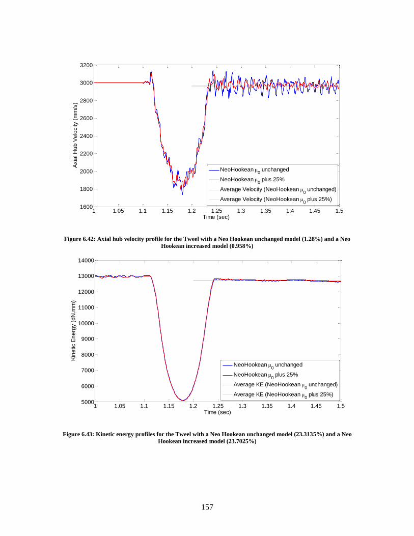
157
Figure 6.42: Axial hub velocity profile for the Tweel with a Neo Hookean unchanged model (1.28%) and a Neo
Hookean increased model (0.958%)
Figure 6.43: Kinetic energy profiles for the Tweel with a Neo Hookean unchanged model (23.3135%) and a Neo
Hookean increased model (23.7025%)
1 1.05 1.1 1.15 1.2 1.25 1.3 1.35 1.4 1.45 1.51600
1800
2000
2200
2400
2600
2800
3000
3200
Time (sec)
Axia
l H
ub
Ve
locity (
mm
/s)
NeoHookean 0 unchanged
NeoHookean 0 plus 25%
Average Velocity (NeoHookean 0 unchanged)
Average Velocity (NeoHookean 0 plus 25%)
1 1.05 1.1 1.15 1.2 1.25 1.3 1.35 1.4 1.45 1.55000
6000
7000
8000
9000
10000
11000
12000
13000
14000
Time (sec)
Kin
etic E
ne
rgy (
dN
.mm
)
NeoHookean 0 unchanged
NeoHookean 0 plus 25%
Average KE (NeoHookean 0 unchanged)
Average KE (NeoHookean 0 plus 25%)

158
6.5 Observations
6.5.1 Reduction in axial hub velocity profile after traversing the obstacle
Figure 6.44: Reduction in axial hub velocity of the Tweel with a Mooney Rivlin unchanged model, Neo Hookean
unchanged model and Marlow properties.
In Figure 6.44, two sets of values have been provided. One set named „Ring‟
refers to the Tweel model with different material models for the ring. The other set
„Spoke‟ refers to the Tweel model with different material models for the spoke. Three
materials have been used for both the ring and the spoke.
When Marlow properties are assigned for the ring and the spokes, it was seen that
the reduction was velocity is 1.265%. On the other hand, the reduction in velocity for an
analytical rigid wheel was 8.04%. This implies that the Tweel with hyperelastic
1.265
1.265
1.22
1.32
1.314
1.28
Ring
Spoke
Percentage reduction in Axial hub velocities after traversing the obstacle
Neo-Hookean Mooney-Rivlin Marlow

159
properties did not lose a lot of energy on impacting an obstacle when compared with an
analytical rigid wheel.
When a Mooney Rivlin unchanged model was used for the ring, the reduction in
velocity turned out to be 1.22%. The Tweel with an unchanged Mooney Rivlin model
rolled with a slightly higher velocity than the Tweel with Marlow properties. On the other
hand, when a Mooney Rivlin unchanged model was used for the spokes, the reduction in
velocity was 1.32%. This signifies that the Tweel with the unchanged Mooney Rivlin
model rolled with a slightly lower velocity than the Tweel with Marlow properties.
By replacing the Marlow properties for the ring to a Neo Hookean unchanged
model, the reduction in velocity was 1.314%. The Tweel with an unchanged Neo
Hookean model rolled with a lesser velocity than the Marlow Tweel. When an unchanged
Neo Hookean model was used for the spokes, the reduction in velocity was recorded as
1.28%. This implies that the Tweel with an unchanged Neo Hookean model for the
spokes rolled with a slightly higher velocity than the Marlow Tweel.
Results show that the reduction in velocity after impacting the obstacle is lower
from the Marlow model when an unchanged Mooney Rivlin model is used for the ring.
Similarly, the reduction in velocity after impacting the obstacle is higher from the
Marlow model when an unchanged Neo Hookean model is used for the ring.

160
Figure 6.45: Comparison of reduction in axial hub velocities for different levels of Mooney Rivlin and Neo
Hookean material models
In Figure 6.45, the reduction in axial hub velocity is compared for different
material models. Four sets of values have been provided. The values in the first set are for
the models of the Tweel with 3 levels of Mooney Rivlin material model for the ring. The
other sets can be explained on similar lines.
When Mooney Rivlin model was used for the ring with three levels, the reduction
in velocity of the Tweel with a Mooney Rivlin increased model for the ring is 1.368%.
The Tweel with an unchanged Mooney Rivlin model had a reduction in velocity of
1.224%. The unchanged model rolled with a higher velocity than the increased model. On
the other hand, the reduced model recorded a reduction in velocity of 1.093%. The
1.224
1.314
1.323
1.28
1.368
1.139
1.338
0.958
1.093
1.87
1.034
2.006
Mooney-Rivlin for the ring
Neo-Hookean for the ring
Mooney-Rivlin for the spokes
Neo-Hookean for the spokes
Percentage reduction in Axial Hub Velocities after traversing the obstacle
minus 25% plus 25% Unchanged
161
reduced model rolled with a higher velocity than both the increased and the unchanged
model.
When Neo Hookean model was used for the ring with three levels, the reduction
in velocity of the Tweel with a Neo Hookean increased model for the ring was 1.139%.
The Tweel with an unchanged Neo Hookean model had a reduction in velocity of
1.314%. The increased model rolled with a higher velocity than the unchanged model. On
the other hand, the reduced model recorded a reduction in velocity of 1.87%. The reduced
model rolled with a lower velocity than both the increased and the unchanged model.
When Mooney Rivlin model was used for the spokes with three levels, the
reduction in velocity of the Tweel with a Mooney Rivlin increased model for the spokes
was 1.338%. The Tweel with an unchanged Mooney Rivlin model had a reduction in
velocity of 1.323%. This shows that the unchanged model rolled with a slightly higher
velocity than the increased model. On the other hand, the reduced model recorded a
reduction in velocity of 1.034%. The reduced model rolled with a higher velocity than
both the increased and the unchanged model.
When Neo Hookean model was used for the spokes with three levels, the
reduction in velocity of the Tweel with a Neo Hookean increased model for the spokes
was 0.958%. The Tweel with an unchanged Neo Hookean model has a reduction in
velocity of 1.28%. This shows that the unchanged model rolled with a lower velocity than
the increased model. On the other hand, the reduced model recorded a reduction in
velocity of 2.006%. The reduced model rolled with a lower velocity than both the
increased and the unchanged model.

162
Results show that the velocity reduced more when the stiffness of the Mooney
Rivlin model for both the ring and the spokes was reduced. When the stiffness for the
Mooney Rivlin model was increased by 25% for both ring and the spokes, the velocity
after traversing the obstacle increased. However, the reduction in velocity was less when
the stiffness of the Neo Hookean model was increased for both ring and the spokes.
Conversely, the final velocity after traversing the obstacle decreased when a Neo
Hookean model with increased shear modulus was used for both the ring and the spokes.
6.5.2 Relative Kinetic energy upon impacting an obstacle
Figure 6.46: Percentage of proportion of energy lost for a Mooney Rivlin unchanged model, Neo Hookean
unchanged model and Marlow properties
In Figure 6.46, two sets of results have been provided. „Ring‟ denotes the
changing material models for the ring. „Spoke‟ denotes the changing material models for
2.35
2.35
2.34
2.53
2.54
2.35
Ring
Spoke
Percentage of proportion of kinetic energy lost upon impacting an obstacle
Neo-Hookean Mooney-Rivlin Marlow

163
the spoke. The proportion of energy loss for the reference model was recorded as
2.3457%.
When the material for the ring was changed to an unchanged Mooney Rivlin
model, the proportion of energy loss was 2.3376%. When the same material was used for
the spokes, the proportion of energy loss was recorded as 2.5258%.
When an unchanged Neo Hookean model is used for the ring, the proportion of
energy lost was 2.5424%. Conversely, the proportion of energy loss was 2.3512% when
the same material was used for the spokes.
On comparing with the reference Marlow model, the proportion of energy loss
decreased when an unchanged Mooney Rivlin model was used for the ring. The
proportion of energy lost increased when the same material was used for the spokes.
The amount of energy lost was higher when an unchanged Neo Hookean model
was used for the ring. But when the same material was used for the spokes, the proportion
of energy lost decreased.

164
Figure 6.47: Percentage difference of the Kinetic energy values between the different Tweel models and the
analytical rigid wheel
In Figure 6.47, there are four sets of values with three levels each. In the first set,
Mooney Rivlin material model is considered for the ring. A similar explanation can be
given for the remaining 3 sets.
In the first set, the proportion of energy lost for an unchanged Mooney Rivlin
model for the ring was recorded as 2.34%. When the stiffness was increased, the
proportion of energy loss increased to 2.48%. The proportion of energy loss reduced to
2.11% when the stiffness was reduced.
In the second set, the proportion of energy lost for an unchanged Neo Hookean
model for the ring is 2.54%. When the stiffness was increased, the proportion of energy
lost reduced to 2.24%. The amount of energy lost increased and the proportion of energy
lost increased to 3.33% when the shear modulus was reduced by 25%.
2.34
2.54
2.53
2.35
2.48
2.24
2.48
1.81
2.11
3.33
1.96
3.65
Mooney-Rivlin for the ring
Neo-Hookean for the ring
Mooney-Rivlin for the spokes
Neo-Hookean for the spokes
Percentage of proportion of kinetic energy lost upon impacting an obstacle
minus 25% plus 25% Unchanged

165
In the third set, when the unchanged Mooney Rivlin model was used for the
spokes, the proportion of energy lost was calculated to be 2.53%. This value decreased to
2.48% when the shear modulus was increased. The proportion of energy lost decreased to
1.96% when the shear modulus was reduced.
In the final set, when the unchanged Neo Hookean model was used for the spokes,
the proportion of energy lost was recorded as 2.35%. It reduced to 1.81% when the shear
modulus was increased by 25%. The proportion of energy lost increased to 3.65% when
the stiffness of the Neo Hookean model was reduced by 25%.
Results show that for Mooney Rivlin, a decrease in shear modulus caused a
decrease in energy loss. Conversely, for Neo Hookean, a decrease in shear modulus
resulted in an increase in energy loss and an increase in shear modulus resulted in a
decrease in energy loss.

166
CHAPTER SEVEN – CONCLUSIONS
7.1 Comparison of Stress-Strain Curves for Hyperelastic Material Models
To study the effect of changes in shear modulus for the ring and spokes while
keeping the ratio of volumetric bulk modulus to shear modulus unchanged, the value of
shear modulus is varied from Mooney-Rivlin and Neo-Hookean models obtained from a
nonlinear least-squares fit of the uni-axial stress-strain data. Upon evaluation of the uni-
axial stress-strain data, the results show that on increasing the shear modulus, the tangent
slope of the normal stress-strain curve increases; whereas with decreasing shear modulus,
the slope decreases. For tensile stresses and strains, the Mooney-Rivlin best matches the
original Marlow material model, compared to the simpler Neo-Hookean model.
However, for large compressive stresses, the Mooney-Rivlin model diverges significantly
from the results obtained with Marlow properties. The simple Neo-Hookean model is
able to fit the Marlow curve better for compression, but is less accurate in tension.
7.2 Study of Material Models on Tweel Load-Deflection
As a result of decreasing shear modulus in of the non-pneumatic tire, the vertical
displacement in the static load-deflection curves increases upon loading. The stiffness is
measured from the slope of the load deflection curve. The stiffness of the Tweel reduced
significantly with the Neo Hookean model, while the stiffness with the Mooney Rivlin
model only slightly decreased. As expected, when the shear modulus was increased, the
stiffness of the Tweel increased and the stiffness decreased when the shear modulus was
decreased. The Tweel models are arranged in the ascending order of their stiffness.
167
7.3 Study of Material Models on Vibration during Rolling
7.3.1 Spoke Vibration
From Figure 5.55, the general trend shown is that the vibration amplitude in the
spokes increased when the Marlow properties are changed to either the fitted Mooney
Rivlin or Neo Hookean models, with the Neo Hookean model giving the largest vibration
amplitudes, especially when Neo Hookean was changed for the spokes. It also appears
from these results that changes to spoke material properties have a more significant
influence on spoke vibration when compared to changes in ring properties. In summary,
the spoke vibration amplitudes for the different material models in the order of increasing
magnitudes are: Marlow < Unchanged Mooney Rivlin < Unchanged Neo Hookean.
From Figure 5.56, a general trend is shown that the spoke vibration decreased
when the stiffness of the Mooney Rivlin and the Neo Hookean models was increased
between the extreme limits of plus and minus 25% change. Conversely, for the extreme
limits, vibration amplitudes increased when the stiffness of the Mooney Rivlin and Neo
Hookean models was reduced. However, it should be noted that in the case of the
unchanged Mooney Rivlin model for the ring, the unchanged gave the smallest amplitude
when compared to both the plus and minus extreme limits tested, thus implying that there
is an optimal value somewhere between the limits. Another instance where an optimal
value occurs can be seen in the Neo Hookean model for the spokes, where the unchanged
spoke vibration amplitude was higher than both the plus and minus stiffness limits. Note

168
also that the unchanged Neo Hookean model for the spokes had the largest amplitude
when compared to all models. In summary, the amplitudes for spoke vibration for the
different materials in order of increasing magnitudes for the four sets of data are:
(a) Mooney Rivlin for ring: Unchanged < +25% < -25%
(b) Neo Hookean for ring: +25% < Unchanged < -25%
(c) Mooney Rivlin for spokes: +25% < Unchanged <-25%
(d) Neo Hookean for spokes: +25% < -25% < Unchanged
7.3.2 Ground Vibration
From Figure 5.57, when considering ground vibration, a trend is shown that the
vibration levels increased when the referenced Marlow model was replaced with a least
square fitted Mooney Rivlin and Neo Hookean models. The Neo Hookean model for both
ring and spokes produced large vibrations compared to both Mooney Rivlin and Marlow
models. The largest ground vibration amplitude occurs with the Neo Hookean model for
the spokes. The ground vibration amplitudes for the different material models in the
order of increasing magnitudes are: Marlow < Unchanged Mooney Rivlin < Unchanged
Neo Hookean.
From Figure 5.58, similar to trends found in the spoke vibration, on varying the
stiffness of the different material models for the ring and the spoke, a trend is shown that
the vibration decreased when the stiffness of the Mooney Rivlin and the Neo Hookean
models was increased from +25% to -25%. Conversely, the vibration increased when the
stiffness decreased between the extreme limits. However, In the case of the Neo-
Hookean material for the ring and Mooney Rivlin for the spokes, the Unchanged stiffness
gave the lowest vibration amplitude, suggesting that a optimal value is somewhere

169
between the plus/minus 25% stiffness limits. Similar to spoke vibration, the unchanged
Neo Hookean model for the spokes had the largest ground vibration amplitude when
compared to all models. The amplitudes for ground vibration for the different materials,
with plus/minus 25% change in stiffness, in order of increasing magnitudes for the four
sets of data are:
(a) Mooney Rivlin for ring: +25% < Unchanged < -25%
(b) Neo Hookean for ring: Unchanged < +25% < -25%
(c) Mooney Rivlin for spokes: Unchanged < +25% < -25%
(d) Neo Hookean for spokes: +25% < -25% < Unchanged
7.4 Energy Loss Study
To study the effects of material changes on energy loss from impact rolling over
obstacles, reduction in axial hub velocities and proportion of energy lost by different
materials models were studied and compared. From Figure 6.16 and Figure 6.17, a
general trend is shown that the axial velocity and kinetic energy of the Tweel after
traversing the obstacle reduced slightly when Marlow properties for the ring were
replaced by a least square curve fit model of Mooney Rivlin. Conversely, these
parameters increased when the same model was used for the spokes. However, when a
least square curve fit Neo Hookean model was used for the ring and spokes, the
parameters increased and decreased respectively. The energy reduction after impact
rolling over the obstacle with height 7.5% of the radius of the Tweel, and for the rolling
speed of 3000 mm/sec, for the different materials in the ring and spokes in order of
increasing energy loss are:
(a) Ring: Neo Hookean < Marlow < Mooney Rivlin,
170
(b) Spokes: Mooney Rivlin < Neo Hookean < Marlow.
When the stiffness of the Tweel with Mooney Rivlin and Neo Hookean material
models was varied, a general trend in the final velocity and kinetic energies after
traversing the obstacle was seen. The final axial velocity and kinetic energy (KE) reduced
when the stiffness of a least square curve fit Mooney Rivlin model was increased for both
the ring and the spokes. Conversely, the values of these parameters increased with the
reduction in stiffness. On the other hand, when the stiffness of the Neo Hookean model
for both ring and spokes was increased, the final velocity and KE increased. A reduction
in the values of the final velocity and KE was seen when the stiffness of the Neo
Hookean model was reduced. The Neo Hookean models with reduced shear modulus for
the ring and the spokes showed the largest reduction in final velocity and KE. It is
inferred that the percentage reduction in velocity and proportion of energy lost are
directly proportional to the final velocity and KE respectively. In summary, the energy
reduction after impact rolling over the obstacle with height 7.5% of the radius of the
Tweel, for the different materials in the ring and spokes, with plus/minus 25% change in
stiffness, in order of increasing energy loss are:
(a) Mooney Rivlin for ring: +25% < Unchanged < -25%
(b) Neo Hookean for ring & spokes: -25% < Unchanged < +25%
(c) Mooney Rivlin for spokes: Unchanged < +25% < -25%
171
7.5 Future Work
In the present work, changes to material stiffness were made independently for
the spoke properties and ring properties. In future work, changes in material stiffness to
both the spoke and ring properties would be done together, rather than separate. This
could provide a more fundamental understanding of the effects of different materials on
the behavior of energy loss and vibration for the Tweel. In addition, the effects of visco-
elastic damping can also be investigated.
For the energy loss after impact rolling over obstacles, the effects of geometric
design parameters such as spoke length and curvature, ring thickness, etc. could be
investigated to optimize the Tweel for low energy loss. Parameter studies on the changes
in energy loss at different rolling speeds and obstacle heights could be investigated.
Effects of reducing ground surface traction, so that slip between the wheel and ground
occurs when traversing the obstacle could also be studied.

172
REFERENCES
1. Rhyne, T. B. and Cron, S. M., „„Development of a Non-Pneumatic Wheel,‟‟ Tire
Science and Technology, TSTCA, Vol. 34, No. 3, July – September 2006, pp.
150-169
2. Cron, S., Use of Connectors in Abaqus/Explicit to Simulate Dynamic Motion
Along a Curved Path, in 2004 ABAQUS User's Conference. 2004.
3. Manga, K.K., 2008, “Computation Method for Solving Spoke Dynamics on High
Speed Rolling Tweel™,” Master‟s Thesis, Clemson University, Clemson, SC.
4. Ramachandran, M., 2008, “Nonlinear Finite Element Analysis of Tweel™
Geometric Parameter Modifications on Spoke Dynamics during High Speed
Rolling” Master‟s Thesis, Clemson University, Clemson, SC.
5. Rutherford, W., 2009, “Use of Orthogonal Arrays for Efficient Evaluation of
Geometric Designs for Reducing Vibration of a Non-Pneumatic Wheel during
High-Speed Rolling,” Master‟s Thesis, Clemson University, Clemson, SC.
6. Bezgam, S., 2009, “Design and analysis of alternating spoke Pair concepts for a
non-pneumatic tire with reduced vibration at High speed rolling”, Master‟s
Thesis, Clemson University, Clemson, SC.
7. Proddaturi, A., ”Robust Parameter Design and Finite Element Analysis for a Non
Pneumatic Tire with Low Vibration”, Master‟s Thesis, Clemson University,
Clemson, SC.
8. Manga, K.K., Thompson, L.L., Ziegert, J.C., Rhyne, T.B., and Cron, S.R.,
"Computational Method to Examine Spoke Dynamics in a High Speed Rolling
Wheel", Paper SAE-2009-01-0071, April 2009.
9. Maya Ramachandran, Shashank Bezgam, Lonny L. Thompson, John C. Ziegert,
Timothy B. Rhyne, Steven M. Cron, “On the effects of edge scalloping for
collapsible spokes in a non-pneumatic wheel during high speed rolling”, ASME
International Mechanical Engineering Congress and Exposition, IMECE2009,
Nov 13-19, 2009, Lake Buena Vista, Florida, USA, ASME Paper IMECE2009-
11342.

173
10. William Rutherford, Shashank Bezgam, Amarnath Proddaturi, Lonny Thompson,
John C. Ziegert , Timothy B. Rhyne, Steven M. Cron, “Use of Orthogonal Arrays
for Efficient Evaluation of Geometric Designs for Reducing Vibration of a Non-
Pneumatic Wheel during High-Speed Rolling”, Presented at the September 2009
Meeting of the Tire Society, to appear in journal Tire Science and Technology,
2010.
11. Steven M. Cron, “Role of Abaqus in the Development of the Michelin Tweel®
Tire”, Proceedings of the 2010 Simulia Users Conference, Providence, Rhode
Island.
12. Abaqus Analysis User Manual
13. http://en.wikipedia.org/wiki/Orthotropic_material
14. Shashank Bezgam, Lonny Thompson, John C. Ziegert , Timothy B. Rhyne,
Steven M. Cron, “Numerical study of vibration of an alternating spoke pair design
concept for a non-pneumatic tire during high-speed rolling”, presented at the 2010
Tire Society meeting, and for consideration for publication in the journal Tire
Science and Technology.
15. http://www.oofem.org/resources/doc/matlibmanual/node6.html
16. http://en.wikipedia.org/wiki/Poisson_ratio
17. ABAQUS CAE/User‟s Manual
18. Meriam J.L. and Kraige, L.G., Dynamics, Wiley, 2007.
19. Abaqus Theory Manual

174
APPENDIX

175
Appendix A:Analytical model of a Rigid Wheel
Consider a rigid wheel of mass „m‟, and outer radius R, rolling over a flat ground
until the wheel impacts an obstacle of height „b‟; see Figure Appendix 1. The center of
gravity for the rigid wheel is denoted by point G, and the point where the wheel comes in
contact with the obstacle is denoted by C.
Appendix 1: Rigid wheel just before the first impact
The rigid wheel impacts twice when it rolls over the obstacle. The first impact is
when the wheel strikes the obstacle and the second impact is when the rigid wheel strikes
the ground after traversing the obstacle. When the wheel first impacts the obstacle, its
motion is assumed to change almost instantaneously from rolling without slip on the
ground to a fixed axis rotation about the point of impact. Let 1( )ch be the angular
momentum about the contact point C just before the first impact and let 2( )ch be the
angular momentum about point C just after the first impact. Assume that there is an
infinitesimal time interval right after impact between the wheel and contact point, in
176
which the wheel does not change position significantly, and does not lose contact with
the round. The angular impulse-momentum equation about point C can be written as,
1 2( ) ( )c c ch M dt h
Neglecting non-impulsive forces, the angular impulse defined by integral term can be
neglected or approximated to zero since the time interval of impact is extremely small,
and the impact force is assumed to have its line of action thru point C. In this case,
angular momentum is conserved about point C, and the above equation is approximated
as,
1 2( ) ( )c ch h
The angular momentum about point C is defined by the angular momentum
1 1 1( ) ( ) ( )c G Gh I m V r b
Assuming no slip condition and using the kinematic equation 1 1( )GV R and 2
G GI mk ,
the above expressions simplifies into,
2
1 1( ) ( ) 1 Gc G
k bh m V R
R R
From Figure Appendix 2, just after impact, the wheel is assumed change direction
such that the direction of velocity is parallel to the tangent to the rigid wheel passing
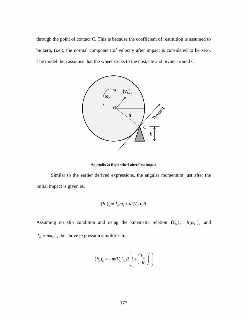
177
through the point of contact C. This is because the coefficient of restitution is assumed to
be zero, (i.e.), the normal component of velocity after impact is considered to be zero.
The model then assumes that the wheel sticks to the obstacle and pivots around C.
Appendix 2: Rigid wheel after first impact
Similar to the earlier derived expressions, the angular momentum just after the
initial impact is given as,
2 2 2( ) ( )c G Gh I m V R
Assuming no slip condition and using the kinematic relation 2 2( ) ( )G GV R and
2
G GI mk , the above expression simplifies to,
2
2 2( ) ( ) 1 Gc G
kh m V R
R

178
From conversion of angular momentum about C, 1 2( ) ( )c ch h , the speed just after impact
can be written in terms of the speed just before impact as;
2 1( ) 1 ( )G G
bV C V
R
where
12
1 GkC
R
This is the velocity of the rigid wheel after the first impact, (i.e.), after it strikes the
obstacle. After traversing the obstacle, the rigid wheel again makes contact with the flat
ground. This is considered to be the second impact. Assuming the wheel pivots about C,
the speed just before impacting the ground 2( )GV is the same as the speed just after the
first impact with direction parallel to the tangent plane rotated 90 degrees about C. The
point of impact when the rigid wheel makes contact with the ground is denoted as P.

179
Appendix 3: Rigid wheel just before the second impact
On neglecting non-impulsive forces and conserving angular momentum about the point
P,
2 3( ) ( )p ph h
The angular momentum just before impact about point P is,
2 2 2( ) ( )p G Gh I m V d
where d = r-b. Using no slip condition 2 2( )GV R , the above expression can be
expressed as
2
2 2( ) ( ) 1Gp G
k bh m V R
R R
Once the wheel impacts the ground, it is assumed once again that the coefficient of
restitution is zero, (i.e.), no bounce or rebound is considered. In such a case, the normal

180
(vertical) speed is zero and hence the rigid wheel is constrained to move horizontally.
Appendix 4 shows the motion of the rigid wheel after impacting the ground.
Appendix 4: Rigid wheel just after the second impact
The angular momentum about P after impact is,
2
3 3( ) ( ) 1 Gp G
kh m V R
R
Using principles of conservation of angular momentum before and after the second
impact, the final velocity with which the rigid wheel travels after traversing the obstacle
is given to be,
2
3 2 1( ) 1 ( ) 1 ( )G G G
b bV C V C V
R R
,
where 2
1
1 G
Ck
R

181
Note the square on the term on the bracket appears due to the two impact events during
wheel traversing the obstacle. Using the notation 1( )i GV V and 3( )f GV V , the relative
change in velocity before impact and after traversing the obstacle is
2
1 1i f
i i
V VV bC
V V R
The rigid-body kinetic energy for general motion of the rigid wheel is given by
2 21 1
2 2K G GE mV I
Assuming no-slip kinematics
/GV R
The kinetic energy can be written as,
2
211
2
GK G
kE m V
R
The initial rigid body kinetic energy is
2
211
2
Gi i
kE m V
R
The final kinetic energy for the rigid wheel after traversing the obstacle is
182
2 2 4
2 21 11 1 1
2 2
G Gf f i
k k bE m V m C V
R R R
Thus the kinetic energy loss is given by,
4
1 1i f
i i
E EE bC
E E R