A concise introduction to quantum probability, quantum mechanics, and

quantum computation

Greg Kuperberg∗

UC Davis, visiting Cornell University

(Dated: 2005)

Quantum mechanics is one of the most interestingand surprising pillars of modern physics. Its basicprecepts require only undergraduate or early grad-uate mathematics; but because quantum mechanicsis surprising, it is more difficult than these prerequi-sites suggest. Moreover, the rigorous and clear rulesof quantum mechanics are sometimes confused withthe more difficult and less rigorous rules of quantumfield theory.

Many working mathematicians have an excellentintuitive grasp of two parent theories of quantummechanics, namely classical mechanics and probabil-ity theory. The empirical interpretations of each ofthese theories — above and beyond their mathemat-ical formalism — have been a great source of ideasfor mathematics proper. I believe that more mathe-maticians could and should learn quantum mechan-ics and borrow its interpretation for mathematicalproblems. Two subdisciplines of mathematics thathave assimilated the precepts of quantum mechan-ics are mathematical physics and operator algebras.However, the prevailing intention of mathematicalphysics is the converse, to apply mathematics toproblems in physics. The theory of operator algebrasis closer to the spirit of this article; in this theory theprecepts of quantum mechanics are sometimes called“non-commutative probability”.

Recently quantum computation has entered as anew reason for both mathematicians and computerscientists to learn the precepts of quantum mechan-ics. Just as randomized algorithms can be moder-ately faster than deterministic algorithms for somecomputational problems (such as testing primality),some problems admit quantum algorithms that arefaster (sometimes much faster) than their classicaland randomized alternatives. These quantum algo-rithms can only run on a new kind of computer calleda quantum computer. As of this writing, convincingquantum computers do not exist. Nonetheless, the-oretical results suggest that quantum computers arepossible rather than impossible. Entirely apart fromits potential as a technology, quantum computationis a beautiful subject that combines mathematics,

∗Electronic address: greg@math.ucdavis.eduandgreg@math.

cornell.edu

physics, and computer science.This article is a concise introduction to quantum

probability theory, quantum mechanics, and quan-tum computation for the mathematically preparedreader. Chapters 2 and 3 depend on Section 1 butnot on each other, so the reader who is interested inquantum computation can go directly from Chap-ter 1 to Chapter 3.

This article owes a great debt to the textbook onquantum computation by Nielsen and Chuang [20],and to the Feynman Lectures, Vol. III [12]. An-other good textbook written for physics students isby Sakurai [21].

Exercises

These exercises are meant to illustrate how empir-ical interpretations can lead to solutions of mathe-matical problems.

1. The probabilistic method: The Ramsey num-ber R(n) is defined as the least R such that ifa simple graph Γ has R vertices, then either itor its complement must have a complete sub-graph with n vertices. By considering randomgraphs, show that

R(n) ≥ 2(n−1)/2

(2(n!))1/n.

2. Angular momentum: Let S be a smooth sur-face of revolution about the z-axis in R3, andlet ~p(t) be a geodesic arc on S, parameterizedby length, that begins at the point (1, 0, 0) att = 0. Show that ~p(t) never reaches any pointwithin 1/|p′y(0)| of the vertical axis.

3. Kirchoff’s laws: Suppose that a unit square istiled by finitely many smaller squares. Showthat the edge lengths are uniquely determinedby the combinatorial structure of the tiling,and that they are rational. (Hint: Build theunit square out of material with unit resistivitywith a battery connected to the top and bot-tom edges. Cut slits along the vertical edges ofthe tiles and affix zero-resistance wires to thehorizontal edges. Each square becomes a unitresistor in an electrical network.)

2

1. QUANTUM PROBABILITY

The precepts of quantum mechanics are neithera set of physical forces nor a geometric model forphysical objects. Rather, they are a variant, andultimately a generalization, of classical probabilitytheory. (This is following the standard Copenhageninterpretation; see Section 1.6.) Quantum proba-bility is usually defined using the matrix mechanicsmodel, which describes vector states (or pure states)and offers a probabilistic interpretation of final mea-surement. We will present this model together withan important extension to mixed states. In physics,wave mechanics is sometimes presented as an alter-nate definition of quantum mechanics; we will de-scribe it as a special case of pure-state matrix me-chanics.

Since classical probability is a major analogy forus, it is reviewed in Section 1.10. In short, we canthink of classical probability as a category Probwhose objects are measure spaces (or in the finitecase, finite sets) and whose morphisms are stochas-tic maps. (For readers who are not comfortable withthis terminology, Section 1.11 is a cursory review.)Even though category theory can be very abstract[18], our interpretation of this category is very em-pirical: A measure space is the natural model for aphysical (or otherwise empirical) object that can bein a random state, and stochastic maps are the ac-tions on such objects that are empirically allowed inclassical probability. Stochastic maps also subsumethe notions of events and random variables. Finally(and crucially) the probability category Prob is atensor category: A Cartesian product of measurespaces, which is in spirit a tensor product, carriesthe joint states of two (or more) separate probabilis-tic objects.

We will define a category Quant for quan-tum probability which is analogous to the cate-gory Prob. The ultimate generalization, discussedin Section 1.8, is a category vN that containsboth Quant and Prob. Its objects are von Neu-mann algebras, which are sometimes called “non-commutative measure spaces”. The objects ofQuant are, famously, Hilbert spaces. Until Sec-tion 1.7, we will consider only finite-dimensional vec-tor spaces. These are enough to learn from, just asthe finite case is enough to learn most of the empir-ical interpretation of classical probability.

1.1. Vector states and unitary maps

Although it lacks some crucial empirical structure,most of quantum mechanics and much of quantumcomputation relies only on a simpler category (than

Quant) which we will call U. The objects of Uare complex Hilbert spaces and the morphisms areunitary maps. We also add subunitary maps to Uto make a moderately larger category U’. We willalso mostly restrict our attention to the subcategoryU<∞ of finite-dimensional Hilbert spaces.

Recall that a Hilbert space is a complex vectorspace H with a positive-definite Hermitian innerproduct 〈·|·〉. This means that 〈·|·〉 is a function fromH → H to C that satisfies these axioms:

〈ψ1 + ψ2|ψ3〉 = 〈ψ1|ψ3〉+ 〈ψ2|ψ3〉〈ψ1|ψ2〉 = 〈ψ2|ψ1〉〈ψ1|αψ2〉 = α〈ψ1|ψ2〉for α ∈ C

〈ψ|ψ〉 > 0 for ψ 6= 0.

(In the infinite case, H must also be complete rela-tive to the norm

||ψ|| =√〈ψ|ψ〉.)

In quantum theory, the traditional notation is |ψ〉 (a“ket”) for ψ and 〈ψ| (a “bra”) for the dual vector

〈ψ| = ψ∗ = 〈ψ|·〉.

If X is an operator on H, then

〈ψ1|X |ψ2〉

is an expression for “the inner product of ψ1 withX(ψ2)”. If

X = |ψ1〉 ⊗ 〈ψ2|

has rank 1, then we can omit the “⊗” and just write

X = |ψ1〉〈ψ2|.

This notation is due to Dirac [10] and is called “bra-ket” notation. A linear map U : H1 → H2 is unitaryif it preserves the inner product 〈·|·〉; it is subunitaryif it preserves or decreases the attendant norm || · ||.Recall also that a linear map from a Hilbert spaceto itself is called an operator.

The standard finite example of a Hilbert space isthe standard complex vector space Cn with the innerproduct

〈~x|~y〉 = x1y1 + x2y2 + · · ·+ xnyn.

We can generalize this to say that for any finite setA, the vector space CA is a Hilbert space with stan-dard orthonormal basis A. Every finite-dimensionalHilbert space is isomorphic to Cn for some n, andtherefore CA for any A with |A| = n.

3

In finite quantum mechanics, as in classical prob-ability, we can define a physical object by specifyinga finite set A of independent configurations. In in-formation theory (both quantum and classical), theobject is often called “Alice”. In the classical case,the set of all normalized states of Alice is the sim-plex ∆A spanned by A in the vector space RA (seeSection 1.10). I.e., a general state has the form

µ =∑

a∈A

pa[a]

for probabilities pa ≥ 0 that sum to 1. (For unnor-malized states, the sum need not be 1.) The numberpa is interpreted as the probability that Alice is instate a. Quantumly, Alice’s set of vector states is thevector space CA. In formulas, a state of this type isa vector

|ψ〉 =∑

a∈A

αa|a〉.

The state |ψ〉 is normalized if

〈ψ|ψ〉 =∑

a∈A

|αa|2 = 1

and subnormalized if the left side is at most 1. Thecoefficient αa is called the amplitude of the quantumstate |a〉 and the square norm |αa|2 is interpreted asthe probability that Alice is in state |a〉. The phaseof αa (i.e., its argument or angle as a complex num-ber) has no direct probabilistic interpretation, but itwill be immediately relevant when we consider op-erations on |ψ〉. More precisely, the relative phaseof two coordinates αa and αa′ is indirectly measur-able. It will turn out that the global phase of |ψ〉is not empirical; Section 1.4 discusses a change informalism that eliminates it.

The state |ψ〉 is also called a quantum superpo-sition, an amplitude function, or a wave function.This last name, perhaps the most common term inphysics, is motivated by the fact that |ψ〉 typicallysatisfies a wave equation in infinite quantum me-chanics (Example 1.7.1 and Section 2.1). It also pre-dates the Copenhagen interpretation and arguablydistracts from it.

If A and B are the configuration sets of two quan-tum systems (“Alice” and “Bob”), then, as we said,an empirical transition from Alice’s state to Bob’sstate is a unitary (or subunitary) map

U : CA → CB.

The requirement that U be linear is the quantumsuperposition principle. It contradicts the similar-looking classical superposition principle: if ampli-tudes add, then probabilities usually do not. (They

will eventually be reconciled.) The entries of Uare also called amplitudes, just as the entries of astochastic map are themselves probabilities. Theunitary condition is interpreted as conservation ofprobability. Since we have posited that |αa|2 is aprobability, U conserves total probability if and onlyif

||Uψ|| = ||ψ||

for all ψ ∈ CA. If U is allowed to extinguish thestate ψ, then in general

||Uψ|| ≤ ||ψ||

for all ψ ∈ CA, i.e., U is subunitary.

i/2

i/2

−i/2

i/2

i/2

i/2

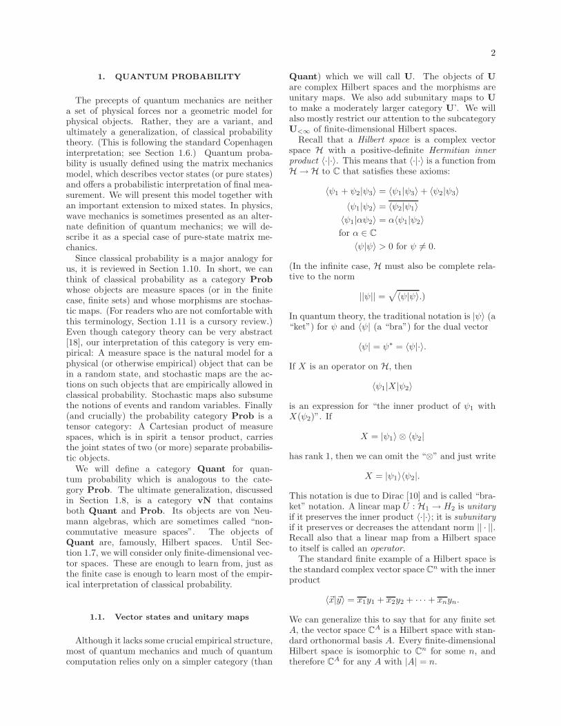
Figure 1: An idealized two-slit experiment.

It is traditional to illustrate the quantum super-position principle in an idealized setting called the“two-slit experiment” (or a more general diffractionexperiment). Figure 1 shows the basic idea: A laseremits photons that can travel through either of twoslits in a grating and then may (or may not) reacha detector. The source has a single state (the stateset A has one element), while the grating has twostates and there are two detectors (B and C eachhave two elements). The transitions for each pho-ton, as it passes from A to B to C, are described bytwo subunitary matrices

U : CA → CB V : CB → CC .

The matrices are

U =

(i2i2

)V =

(i2

i2

i2 − i

2

),

and

V U =

(− 1

20

).

The total amplitude of the photon reaching the topdetector is − 1

2 and the probability is 14 ; this case

is called constructive interference. The total ampli-tude reaching the bottom detector is 0, so the photonnever reaches it; this case is called destructive in-terference. On the other hand, if one of the slits of

4

blocked, then we can discard one of the states in |B|,with the result that each detector is reached withprobability 1

16 . The classical superposition principle

would dictate a probability of 18 for each detector

with both slits open; thus it is violated.

i/2

i/2

±i/2

i/2

Figure 2: An angle-dependent detector in the two-slitexperiment.

A natural reaction to the violation of classical su-perposition is to try to determine which slit the pho-ton went through. One way to do so is to use a de-tector which is sensitive to the angle that the photoncomes in, as in Figure 2. But then this detector rep-resents two distinct states rather than one. Thus thefinal state vector is

|ψ〉 =

(− 1

4± 1

4

)

and its total probability is

〈ψ|ψ〉 = ||ψ||2 =1

8,

regardless of the phases of path segments to andfrom the slits. The broader lesson is that amplitudesof different trajectories of an object only add whenthere is no evidence of which trajectory it took; oth-erwise the probabilities add. If we want to see quan-tum superposition, it is not enough to wittingly orunwittingly ignores such evidence. Rather, if the twotrajectories induce different states of the universe,so that some observer could in principle distinguishthem, then they obey classical superposition. More-over, the effect is not the result of interaction be-tween photons; photons do not interact with eachother1. Indeed, the laser could be tuned to shootonly one photon at a time. Of course, our two-slit“experiment” is only an idealization of a real exper-iment; but see Sections 1.3 and 1.6.

Examples 1.1.1. A qubit is a two-state quantumobject with configuration set {0, 1}. Two of their

1 More precisely, detecting photon-photon interactions re-quires enormous particle accelerators.

quantum superpositions are:

|+〉 =|0〉+ |1〉√

2|−〉 =

|0〉 − |1〉√2

Both of these states have probability 12 of being in

either configuration |0〉 or |1〉, but they are differ-ent states. This is demonstrated by the effect of aunitary operator H called the Hadamard gate:

H =

(1 11 −1

).

It exchanges |0〉 with |+〉 and |1〉 with |−〉.The spin state of a spin- 1

2 particle is a two-statesystem which is important in physics. (Electrons,protons, and neutrons are all spin- 1

2 particles.) Theconventional orthonormal basis is |↑〉 (“spin up”) and|↓〉 (“spin down”). The names of the states refer tothe property of the electron spinning (according tothe right-hand rule) about a vertical axis in thesetwo states. Even though a rotated electron is stillan electron, this configuration set for it does not ro-tate to itself; neither does any other. The resolutionof this paradox is that rotated states appear as su-perpositions. For example, the states “spin left” and“spin right” are analogous to |+〉 and |−〉:

|→〉 =|↑〉+ |↓〉√

2|←〉 =

|↑〉 − |↓〉√2

.

Exercises

1. Suppose that the lengths of the entries of acomplex matrix U are all fixed, but the phasesare all chosen uniformly randomly. (If you like,you can also suppose that for any choice of theamplitudes, U is subunitary.) Show that onaverage, each entry of U |ψ〉 satisfies the clas-sical superposition principle.

2. If U is a matrix, then the matrix

Mab = |Uab|2

can be called dephasing of U . A dephasing ofa unitary matrix is always doubly stochastic,meaning that the entries are non-negative andthe rows and columns add to 1. Find a 3 ×3 doubly stochastic matrix which is not thedephasing of any unitary matrix.

3. Show that every n × k subunitary matrix Ucan be extended to an (n+k)×(n+k) unitarymatrix V :

V =

(U ∗∗ ∗

).

5

Show that V cannot usually have order lessthan n+ k.

4. If U1, U2, . . . , Un are unitary operators, theneach entry of their product

U = Un . . . U2U1

can be expressed as a sum of products of en-tries of the factors:

〈an|Un . . . U2U1|a0〉=

∑

a0,a1,...,an

〈an|Un|an−1〉 . . . 〈a2|U1|a1〉〈a1|U1|a0〉.

Such an expansion is interpreted as path sum-mation; it is the same idea as a sum over his-tories in classical probability.

For example, let n = 4 and let each

Uk =1√2

(1 1

−1 1

).

Find the amplitudes of the 16 paths and groupthem according to how they sum.

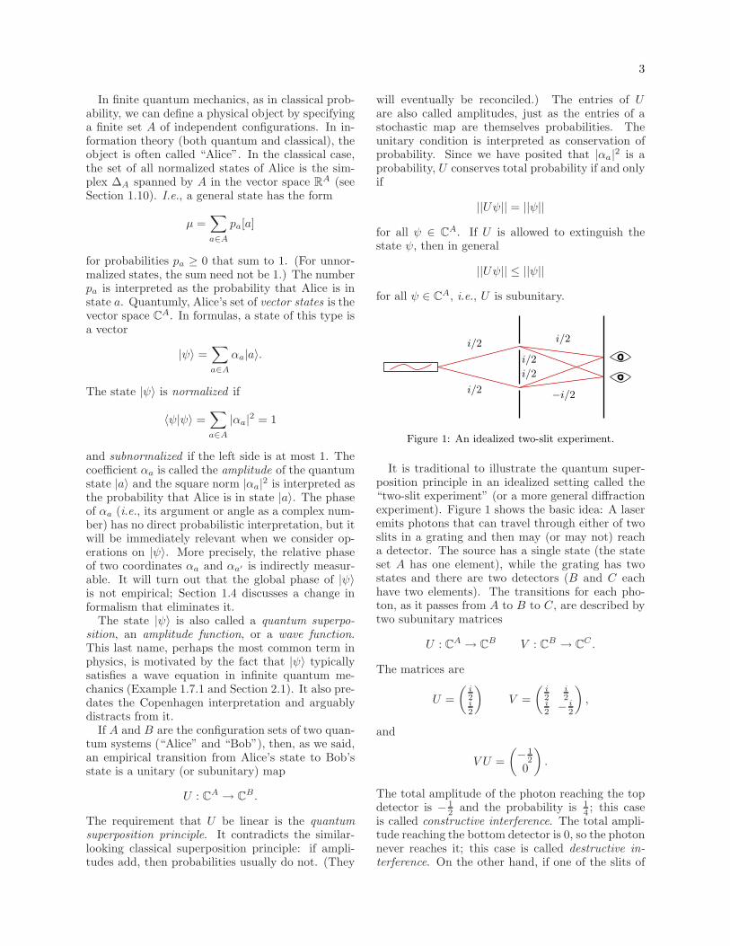
5. In general for a spin- 12 particle, the state

|~v〉 = α|↑〉+ β|↓〉

spins in the direction

~v = (Re αβ, Im αβ, |α|2 − |β|2).

Check that this is a unit vector when |~v〉 isnormalized, and that every unit vector in R3 isachieved. This formula is therefore a surjectivefunction from the unit 3-sphere S3 ⊂ C2 to the2-sphere S2 ⊂ R3. What is its usual name inmathematics?

1.2. Measurements and basis independence

Suppose that H (or H = CA) is the Hilbert spaceof a quantum object, and that the object is in thestate |ψ〉 ∈ H. A measurement or real-valued quan-tum random variable is a Hermitian operator X onH. The eigenvalues of X are interpreted as its rangeas a random variable. (Since we are assuming thatH is finite-dimensional, X admits a complete set oforthogonal eigenvectors. For the infinite case seeSection 1.7.) The assertion that X = λ as a randomvariable is interpreted as the condition that |ψ〉 is aneigenvector of X with eigenvalue λ. More generally,for any |ψ〉, the probability that X = λ is given bythe formula

P [X = λ] = 〈ψ|Pλ|ψ〉,

where Pλ is the orthogonal projection onto theeigenspace of λ. (Note that this probability does notdepend on the global phase of |ψ〉.) Moreover, if thevalue λ is measured, the conditional state afterwardis

|ψ′〉 =Pλ|ψ〉√〈ψ|Pλ|ψ〉

.

Conditioning on a measurement is also called “statecollapse” or “wave function collapse”.

This abstract definition of a measurement, and thereferences to abstract Hilbert spaces, can be moti-vated by the more concrete discussion in Section 1.1,and they lead to a better presentation of unitaryquantum probability. In Section 1.1, we tacitly ac-cepted that if H = CA is Alice’s state space, thenone kind of a valid measurement is whether Alice isin the configuration a ∈ A, and we said that its prob-ability of this is the square amplitude |αa|2. Moregenerally, if D : A→ S is some function, then

P [D = s] =∑

D(a)=s

|αa|2;

this was implied by the discussion about distinct andidentical states. But, taking S = R, the functionD uniquely extends to a Hermitian operator on Hwhich is diagonal in the basis A. At the same time,we posited that unitary operators represent the em-pirical operations on Alice. Since every Hermitianoperator X is diagonalized by a unitary operator,

X = U−1DU,

we can think of a general measurement X as a mea-surement of Alice’s configuration a ∈ A after Aliceis prepared by the transition map U .

Example 1.2.1. Consider a spin- 12 particle and let

Jx =

(0 1

1 0

)Jz =

(1 0

0 −1

)

be two Hermitian operators, given as matrices in thestandard basis {↑, ↓}. These operators measure theparticle’s spin in horizontal and vertical directions.If Jz is definite, then the spin state is either |↑〉 or|↓〉. Both of these states are superpositions of |←〉and |→〉, so if Jz is definite, Jx is not; rather, ithas a 1

2 chance of being either 1 or −1. If Jx ismeasured, then the particle’s state becomes one ofthe two conditional states |←〉 or |→〉, after whichJz is no longer definite; its old value is forgotten.

This example illustrates that every state of aquantum system is a source of randomness; everystate is indefinite. The popular paraphrase of Ein-stein, “God does not play dice with the universe,”refers to this principle.

6

By the same token, if H is the Hilbert space of aquantum object, we can think of any orthonormalbasis A of H as its configuration set. Two com-pletely different orthonormal bases can be equallyempirical; a very important part of empirical think-ing in quantum theory is to be able to change fromone orthonormal basis to another. In physics such achange of description is often called a “duality”. Forexample, one form of particle-wave duality (namely,second quantization of bosons) is very similar to anorthonormal change of basis (Section 2.6).

Example 1.2.2. We can now have a second un-derstanding of a qubit as a quantum object with atwo-dimensional Hilbert space H. We can label anyorthonormal basis |0〉 and |1〉, or we can choose notto distinguish any particular basis. For example,one person’s |0〉 and |1〉 may be another person’s|+〉 and |−〉. One important quantum algorithm,the Grover search algorithm (Section ??) alternatesbetween (dilated) classical computations in the twobases.

A spin- 12 particle illustrates the same point more

geometrically. As it happens, every orthonormal ba-sis of its spin state space consists of the positiveand negative spin states in some direction. But themodel of a qubit as a spin- 1

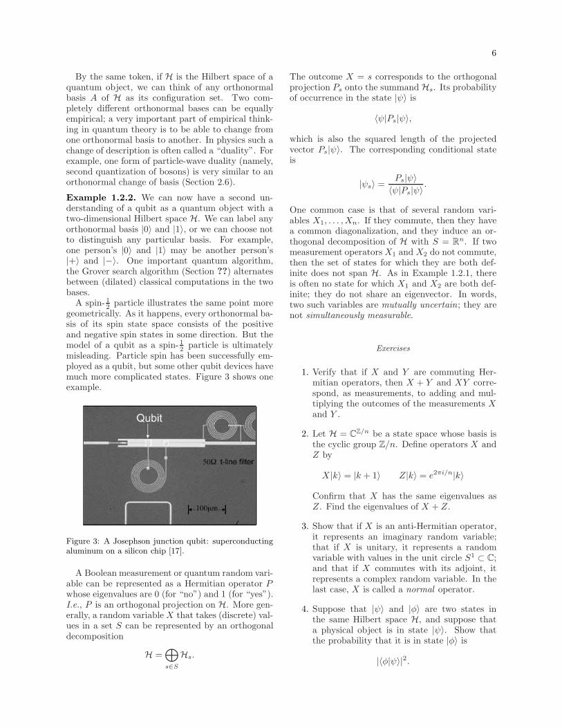
2 particle is ultimatelymisleading. Particle spin has been successfully em-ployed as a qubit, but some other qubit devices havemuch more complicated states. Figure 3 shows oneexample.

Figure 3: A Josephson junction qubit: superconductingaluminum on a silicon chip [17].

A Boolean measurement or quantum random vari-able can be represented as a Hermitian operator Pwhose eigenvalues are 0 (for “no”) and 1 (for “yes”).I.e., P is an orthogonal projection on H. More gen-erally, a random variable X that takes (discrete) val-ues in a set S can be represented by an orthogonaldecomposition

H =⊕

s∈S

Hs.

The outcome X = s corresponds to the orthogonalprojection Ps onto the summand Hs. Its probabilityof occurrence in the state |ψ〉 is

〈ψ|Ps|ψ〉,

which is also the squared length of the projectedvector Ps|ψ〉. The corresponding conditional stateis

|ψs〉 =Ps|ψ〉〈ψ|Ps|ψ〉

.

One common case is that of several random vari-ables X1, . . . , Xn. If they commute, then they havea common diagonalization, and they induce an or-thogonal decomposition of H with S = Rn. If twomeasurement operators X1 and X2 do not commute,then the set of states for which they are both def-inite does not span H. As in Example 1.2.1, thereis often no state for which X1 and X2 are both def-inite; they do not share an eigenvector. In words,two such variables are mutually uncertain; they arenot simultaneously measurable.

Exercises

1. Verify that if X and Y are commuting Her-mitian operators, then X + Y and XY corre-spond, as measurements, to adding and mul-tiplying the outcomes of the measurements Xand Y .

2. Let H = CZ/n be a state space whose basis isthe cyclic group Z/n. Define operators X andZ by

X |k〉 = |k + 1〉 Z|k〉 = e2πi/n|k〉

Confirm that X has the same eigenvalues asZ. Find the eigenvalues of X + Z.

3. Show that if X is an anti-Hermitian operator,it represents an imaginary random variable;that if X is unitary, it represents a randomvariable with values in the unit circle S1 ⊂ C;and that if X commutes with its adjoint, itrepresents a complex random variable. In thelast case, X is called a normal operator.

4. Suppose that |ψ〉 and |φ〉 are two states inthe same Hilbert space H, and suppose thata physical object is in state |ψ〉. Show thatthe probability that it is in state |φ〉 is

|〈φ|ψ〉|2.

7

5. Following Exercise 1.1.5, show that every or-thonormal basis of the spin- 1

2 Hilbert spaceconsists of two spin states that point in op-posite directions.

6. Show that a state |ψ〉 which is simultaneouslydefinite for two Hermitian operators X and Ylies in the kernel of the commutator

[X,Y ] = XY − Y X.

Show that these states span ker[X,Y ] when Xand Y commute with [X,Y ], but not in gen-eral.

7. Show that if a measurement X is performed ona state ψ, its expectation (or average value) isgiven by:

E[X ] = 〈ψ|X |ψ〉.

8. Suppose that X and Y are Hermitian opera-tors on a Hilbert spaceH with a state ρ. Recallthat if X is a classical random variable,

V [X ] = E[X2]− E[X ]2

denotes the variance of X . Prove the general-ized Heisenberg uncertainty relation:

V [X ]V [Y ] ≥ E[i[X,Y ]]2

4.

(Hint: After subtracting the means from Xand Y , show that the 2× 2 matrix

(E[X2] E[XY ]

E[Y X ] E[Y 2]

)

is positive semi-definite. The expectation for-mula in Exercise 1.2.7 is reasonable for arbi-trary operators, not just normal ones.)

1.3. Joint states

Up until this point, a skeptic could still view quan-tum “probability” as kind of a cloud model and notreally a modification of probability theory itself. Ifa configuration set A of a particle is a set of po-sitions, then perhaps the particle is merely diffuse,like a cloud. Quantum superposition, measurement,and equivalence between different orthonormal basesare all surprising, but they are not quite show stop-pers. The topic of this section, namely the correctmodel of joint quantum states, radically contradictsthe cloud interpretation. (Section 1.6 has a moreconclusive result in this direction.)

If A and B are finite configuration sets for twoclassical systems, then the configuration set for thejoint system is the Cartesian product A×B. Equiv-alently, the state space of the joint system is a tensorproduct:

RA ⊗ RB ∼= R[A×B].

This definition extends to the quantum case: If twoquantum systems have state spaces HA and HB,then the joint system has state space HA ⊗HB. Inparticular if A and B are orthogonal bases of HA

and HB (i.e., configuration sets for Alice and Bob),then A × B is a joint basis, just as in the classicalcase. (But see Section 2.4.)

If a quantum object were somehow a cloud of am-plitudes or probabilities, we would expect Alice andBob to have independent states |ψA〉 and |ψB〉, atleast if they were physically separated. When thishappens, their joint state is |ψA〉 ⊗ |ψB〉; this is alsocalled a product state. But most states are not prod-uct states; these states are called entangled. Entan-gled quantum states are evidently similar to corre-lated classical states.

Examples 1.3.1. Since a qubit has the configura-tion set |0〉 and |1〉, a system of n qubits has config-uration set {0, 1}n. Thus the general state for thissystem has 2n amplitudes; for example the generalthree-qubit state is

|ψ〉 = a000|000〉+a001|001〉+a010|010〉+a011|011〉+ a100|100〉+ a101|101〉+ a110|110〉+ a111|111〉.

It may look as if an n-qubit state carries an expo-nential amount of information, namely its 2n ampli-tudes, but this is only true in a weak sense. Withrespect to a reasonable definition of information (seeExercise 1.4.5 and Section 1.8), a quantum superpo-sition is not a record of its list of amplitudes, just asa hand of poker is not a record its

(525

)probabilities.

One important product state on n qubits is theconstant state:

|ψ〉 = |+ + . . .+〉 = 2−n/2∑

s∈{0,1}n

|s〉.

One important entangled state is the cat state (asin “Schrodinger’s cat”):

|ψ〉 =|00 . . . 0〉+ |11 . . . 1〉√

2.

As another example, an EPR pair (see Sec-tion 1.6.2) is a pair of electrons or other elementaryparticles in the entangled spin

|ψ〉 =|↑↓〉 − |↓↑〉√

2.

8

It is similar to the cat state with n = 2. In generalany state one two qubits of the form

|ψ〉 =|a, b〉+ |c, d〉√

2

with

〈a|c〉 = 〈b|d〉 = 0

is called a Bell state or a Bell pair.

Unitary transitions and Hermitian measurementson a joint system |ψA〉⊗|ψB〉 which affect only Alice(respectively Bob) take the form X⊗I (respectivelyI ⊗ X), where X is unitary or Hermitian. This isexactly analogous to the classical case. Such opera-tions are also called local to Alice or Bob.

The combined model of unitary transitions, Her-mitian measurements, and tensor products for jointstates describes an isolated quantum object whosestate is measured after a period of evolution. It isthe standard description of quantum mechanics inmany physics courses. It also describes a unitaryquantum computer that is alternately manipulatedand interrogated by a classical controller. But italso has shortcomings and omissions which confuseits interpretation, namely:

1. Hermitian measurements are missing from theunitary category U. In physical terms, themodel does not include observers, even thoughobservers can also be observed. (But notethat a Boolean measurement P is subunitary;conditioning without normalization does lie inU’.)

2. Many physical objects, including typical ob-servers, are effectively classical, even if they areprima facie quantum. These are also missingfrom the category U.

3. The category U is only weakly connected:there is no strictly unitary map from HA toHB when

dimHA > dimHB.

The subunitary category U’ is strongly con-nected, but a subunitary map from HA to HB

then includes extinction. In other words, in thecategory U’, if Alice has more states than Bob,she cannot transfer her state to Bob withoutthe possibility that the world ends.

4. There is no notion of marginals: If Alice andBob are in an entangled state, there is no vec-tor state for Alice alone. In particular, Alicecan entangle with the environment (“Eve”).

5. Even though measurements are a source ofrandomness, the category Ucannot expressclassical randomness. For example, if the spinstate of an electron is prepared by randomlychoosing between |↑〉 and |↓〉, what is its state?The model of probability distributions on themanifold of vector states of an object is sus-pect, and in the end, redundant.

Sections 1.4 and 1.5 describe another model ofquantum probability, the category Quant, that ad-dresses most of these problems. Section 1.8 describesa final model, the category vN, that settles themmore completely.

Exercises

1. Another description of the EPR state in Ex-amples 1.3.1 is via measurement. Let H havethe spin basis |↑〉 and |↓〉 and define the oper-ators

J totx = Jx ⊗ I + I ⊗ Jx J tot

z = Jz ⊗ I + I ⊗ Jz

on H ⊗ H, where Jx and Jz are defined asin Example 1.2.1. Show that J tot

x and J totz

have one common eigenstate, for which botheigenvalues vanish.

2. Show that if H is a Hilbert space of dimensionat least 2, there does not exist a linear map

U : H → H⊗H

that takes every state |ψ〉 to a state equivalentto |ψ〉⊗ |ψ〉. (Recall that two states are equiv-alent if they differ by a global phase.) This isthe simplest of a series of no cloning theoremsfor quantum states. A harder version: Showthat such a map U is not even approximatelylinear.

3. Show if |ψ〉 and |φ〉 are two Bell states sharedby Alice and Bob, then there is a unitary op-erator local to Alice (i.e., of the form U ⊗ I)which takes |ψ〉 to |φ〉:

(U ⊗ I)|ψ〉 = |φ〉.

Thus all Bell states are equivalent.

4. Show that if |ψ〉 ∈ HA ⊗HB is a vector stateand

dimHA ≤ dimHB,

then it has the form

|ψ〉 =∑

a∈A

αa|a〉 ⊗ |f(a)〉

9

for some orthonormal bases A and B and somefunction f : A → B. This presentation iscalled a Schmidt decomposition of |ψ〉. Showthat the unordered set of numbers |αa|2 isuniquely determined by |ψ〉.

5. A common error in quantum probability is tomistake the direct sum HA ⊕HB for the jointstate space of Alice and Bob. Provide an em-pirical interpretation for direct sums which,among other properties, would also work inclassical probability.

6. Show that the cat states from Examples 1.3.1are entangled.

1.4. Operator states

Let H be the (finite-dimensional) Hilbert spaceof a quantum object, Alice. We define an opera-tor state of Alice (or more simply a state) to be apositive semi-definite Hermitian operator ρ on H.(Positive semi-definiteness is denoted ρ ≥ 0.) Thestate ρ is normalized if Tr(ρ) = 1 and subnormalizedif Tr(ρ) ≤ 1. In this section and the next one wewill define a new model (the category Quant<∞) ofquantum probability by replacing vector states withoperator states, and by replacing unitary operatorsby a more complete class of quantum operations,analogous to stochastic maps.

LetM(H) be the vector space of all operators onH. (Later we will abbreviate the algebra of n × nmatrices M(Cn) as Mn.) The set

M+,1(H) ⊂M(H)

of all normalized states is the Bloch region of Alice.Also let M+,≤1(H) be the set of all subnormalizedstates and let M+(H) be the set of all states.

Proposition 1.4.1. If H is an n-dimensionalHilbert space thenM+,1(H) is a compact and convexset of real dimension n2− 1. Its extremal points arerank 1 operators: If ρ is extremal, it has the form

ρ = |ψ〉〈ψ|

for a unit vector |ψ〉 ∈ Cn.

The Bloch region M+,1(H) is analogous to theclassical simplex ∆A of probability distributions ona finite set A. (Section 1.8 will discuss a mutualgeneralization.) First, the positivity and normaliza-tion conditions that define the two regions are bothmathematically similar and have similar interpreta-tions. If we choose an orthonormal basis A for H,

then an operator state ρ becomes a matrix; it canbe written

ρ =∑

a,a′∈A

pa,a′ |a〉〈a′|.

The diagonal entry pa,a is the probability of the con-figuration |a〉. Thus the positivity condition ρ ≥ 0asserts that the probability of any configuration (inany basis) is non-negative. The normalization con-dition asserts that the total probability in any basisis 1:

Tr(ρ) =∑

a∈A

pa,a = 1;

evidently this condition is basis-independent. Be-cause the diagonal entries of ρ are probabilities, it isoften called a density matrix or a density operatorin physics.

The geometric features of M+,1(H) and ∆S arealso similar, albeit with some important differencesas well. Both regions are convex in order to allowclassical superpositions. More precisely, if ρ1 and ρ2

are two states and 0 < p < 1 is a probability, thenthe state

ρ = pρ1 + (1− p)ρ2 (1)

is a classical superposition or mixture of ρ1 and ρ2;it can be prepared by choosing randomly betweenthem. If ρ is a mixture, i.e.if it is not an extremalpoint ofM+,1(H), then it is also called a mixed state.

If a state µ ∈ ∆S is extremal, then it is an ele-ment of S itself. It can then be called definite inthe sense µ possesses no randomness: the proba-bility of every event is either 0 or 1. If a stateρ ∈ M+,1(H) is extremal, then it is called pure.By Proposition 1.4.1, pure states correspond to vec-tor states, except that |ψ〉〈ψ| does not depend onthe global phase of |ψ〉. As in Example 1.2.1, everystate M+,1(H) is a source of randomness; all statesare indefinite.

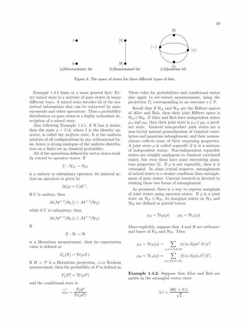
Example 1.4.1. Our third and final understand-ing of a qubit is set of states is the Bloch regionM+,1(H). In this caseM+,1(H) is a round ball andis called the Bloch sphere, as shown in Figure 4. Twopure states are orthogonal if and only if they are an-tipodal as points on the Bloch sphere. The state inthe middle,

ρ =|0〉+ |1〉

2,

is the uniform state; it is the equal mixture of anytwo orthonormal states.

10

0

1

(a)Deterministic bit

[0]

[1]

(b)Randomized bit

|0〉

|1〉

|+〉|−〉

(c)Quantum bit

Figure 4: The space of states for three different types of bits.

Example 1.4.1 hints at a more general fact: Ev-ery mixed state is a mixture of pure states in manydifferent ways. A mixed state encodes all of the sta-tistical information that can be extracted by mea-surements and other operations. Thus a probabilitydistribution on pure states is a highly redundant de-scription of a mixed state.

Also following Example 1.4.1, if H has d states,then the state ρ = I/d, where I is the identity op-erator, is called the uniform state. It is the uniformmixture of all configurations in any orthonormal ba-sis, hence a strong analogue of the uniform distribu-tion on a finite set in classical probability.

All of the operations defined for vector states read-ily extend to operator states. If

U : HA →HB

is a unitary or subunitary operator, its induced ac-tion on operators is given by

U(ρ) = UρU∗.

If U is unitary, then

U(M+,1(H1)) ⊂M+,1(H2),

while if U is subunitary, then

U(M+,1(H1)) ⊂M+,1(H2).

If

X : H → H

is a Hermitian measurement, then its expectationvalue is defined as

Eρ[X ] = Tr(ρX).

If H = P is a Hermitian projection, i.e.a Booleanmeasurement, then the probability of P is defined as

Pρ[P ] = Tr(ρP )

and the conditional state is

ρ|P =PρP

Tr(ρP ).

These rules for probabilities and conditional statesalso apply to set-valued measurements, using theprojection Ps corresponding to an outcome s ∈ S.

Recall that if HA and HB are the Hilbert spacesof Alice and Bob, then their joint Hilbert space isHA⊗HB . If Alice and Bob have independent statesρA and ρB, then their joint state is ρA⊗ρB, a prod-uct state. General non-product joint states are anon-trivial mutual generalization of classical corre-lation and quantum entanglement, and their nomen-clature reflects some of their surprising properties.A joint state ρ is called separable if it is a mixtureof independent states. Non-independent separablestates are roughly analogous to classical correlatedstates, but even these have some interesting quan-tum properties [5]. If ρ is not separable, then it isentangled. In some crucial respects, entanglementof mixed states is a weaker condition than entangle-ment of pure states. Current research is devoted torelating these two forms of entanglement.

As promised, there is a way to express marginalsof joint states using operator states. If ρ is a jointstate on HA ⊗ HB, its marginal states on HA andHB are defined as partial traces:

ρA = TrB(ρ) ρB = TrA(ρ).

More explicitly, suppose that A and B are orthonor-mal bases of HA and HB. Then

ρA = TrB(ρ) =∑

a,a′∈A;b∈B

|a〉〈a, b|ρ|a′, b〉〈a′|

ρB = TrA(ρ) =∑

a∈A;b,b′∈B,

|b〉〈a, b|ρ|a, b′〉〈b′|.

Example 1.4.2. Suppose that Alice and Bob arequbits in the entangled vector state

|ψ〉 =|00〉+ |11〉√

2.

11

The operator form of this state is then

ρ = |ψ〉〈ψ| = 1

2

1 0 0 1

0 0 0 0

0 0 0 0

1 0 0 1

.

Both of its marginals are the uniform state:

ρA = ρB =1

2

(1 0

0 1

).

Whereas in classical probability, a marginal of a def-inite state is definite, in quantum probability themarginal of a pure state need not be pure.

In general a linear map

E :M(HA)→M(HB)

is called a superoperator. If we interpret a unitarymap (including both dimension-preserving operatorsand dimension-increasing embeddings) as a super-operator, and we have described a partial trace asanother kind of superoperator. Both of these op-erations are empirical, and we can naively considerthe category that they generate inside the categoryof all superoperators. For the moment we will callit Quant; in the next section we will show that itincludes all maps of states that could reasonably beempirical.

Exercises

1. Verify that a local measurement X⊗ I appliedto a state ρ on a joint system HA ⊗ HB hasthe same probabilities as the measurement Xapplied to the marginal state TrB(ρ), and thatthe conditioned states are also consistent.

2. Prove Proposition 1.4.1.

3. Show, as Example 1.4.1 claims, thatM+,12 is a

round 3-dimensional ball and that pure statesare orthonormal if and only if they are antipo-dal. Show that the probability of any Booleanmeasurement on a state ρ is proportional tothe displacement of ρ from some hyperplanepassing through the center ofM+,1

2 .

4. Show that every state ρ ∈ M+,1n is a convex

combination of at most n pure states that havethe same diagonal entries as ρ.

5. The entropy S(ρ) of a state ρ is defined asTr(ρ(log ρ)). Show that the uniform state I/dmaximizes the entropy S onM+,1

n . Show thata state is pure if and only if it has no entropy.

6. Verify that a pure state conditioned on a mea-surement is still pure. More generally, showthat measurement does not increase entropy:For any projection P and any state ρ,

S(PρP ) ≤ S(ρ).

7. Show that the each marginal of a pure jointstate |ψ〉 ∈ HA ⊗HB is pure if and only if |ψ〉is unentangled.

8. A purification of a state ρ on H is a pure stateon a joint system H⊗H′ whose left marginalis ρ. Show that every state on H has a purifi-cation in H⊗H, and that it is unique up to aunitary operator local to the second factor.

9. The support of a state ρ on H is its image inH as a linear operator. Show that if ρ has fullsupport, then every outcome of a projectivemeasurement has non-zero probability.

10. Show that the uniform state on H is the onlyone which is invariant under all unitary opera-tors onH. Show, following Exercise 1.1.5, thatthe uniform spin- 1

2 state is the only state thatis not direction-dependent.

11. Show that every state in an open neighborhoodof the uniform state on HA⊗HB is separable.

12. Given a joint Hilbert spaceHA⊗HB, computethe dimension (in terms of the dimensions ofHA and HB) of:

a) the space of all joint states on HA ⊗HB.

b) the space of all joint pure states.

c) the space of all product states.

d) the space of all pure product states.

13. This exercise requires knowledge of sometopology and differential geometry. Show thatthe space of pure states of an n-dimensionalHilbert space H is a 2n− 2-dimensional man-ifold, explicitly the manifold CPn−1. Showthat the Riemannian metric that it inheritsfrom its embedding in M(H) is two-point ho-mogeneous, meaning that isometries act tra-sitively on unit tangent vectors. Show that theRiemannian metric (which is called the Fubini-Study metric) is positively curved.

1.5. Quantum operations

This section is mathematically more challengingthan previous sections in Chapter 1. Our goal is tocharacterize all maps

E :M(HA)→M(HB)

12

that satisfy relatively weak conditions that we mightwant from empirical operations. A map that satis-fies them will be called a “quantum operation”. Wewill abbreviateM(HA) asMA for Alice’s operators,MB for Bob’s, etc.

By the classical superposition principle, an empir-ical map

E :MA →MB

should first be a linear map, i.e., a superoperator. IfE is linear, it is called positive if

ρ ≥ 0 =⇒ E(ρ) ≥ 0

and trace-preserving if

Tr(ρ) = 1 =⇒ Tr(E(ρ)) = 1.

Thus the condition that

E(M+,1(HA)) ⊂ E(M+,1(HB))

says that E is positive and trace-preserving or TPP.(Likewise E is positive if it preserves all states andpositive, sub-trace-preserving or PSTP if it preservessubnormalized states.) By analogy with stochasticmatrices, it is tempting to propose TPP maps asquantum operations. However, the tensor product oftwo TPP maps need not be positive, so the categoryof TPP maps is not compatible with joint states asthey are defined in Section 1.3.

A map E : MA → MB is called completely posi-tive (CP) if for every quantum system C, the map

E ⊗ I :MA ⊗MC →MB ⊗MC

is positive, where I is the identity on MC .

Example 1.5.1. The transpose map T : ρ 7→ ρT onMn for n ≥ 2 is positive but not completely positive.

Completely positive, trace-preserving (TPCP)maps do form a tensor category which for the mo-ment we will call Quant. Every quantum operationshould be TPCP; the category Quant should con-tain the empirical class Quant of quantum opera-tions. (If extinction is allowed, then every quantumoperation should be STPCP.) In Section 1.4, we de-fined a category Quant generated by unitary mapsand partial traces; it should be contained in the em-pirical class Quant. The important result is that

Quant = Quant,

which justifies either one as a definition of Quant.We can likewise define Quant′ as the category ofSTPCP maps and Quant+ as the category of CPmaps.

Theorem 1.5.1 (Stinespring,Kraus). Let

E :MA →MB

be a superoperator. Then E is completely positive ifand only if there exist operators

E1, . . . , EN : HA →HB

such that

E(ρ) =

N∑

k=1

EkρE∗k . (2)

Equivalently E factors as

MAU→MB ⊗MC

TrC→ MB,

where

D(ρ) = DρD∗

and TrC is a partial trace.The map E is trace-preserving if and only if

N∑

k=1

E∗kEk = I ∈MA, (3)

in which case D is unitary.

Often Theorem 1.5.1 is called Stinespring’s the-orem [23]. Equation (2) is called the operator-sumrepresentation or the Kraus decomposition [16]. Theoperation D, or the corresponding operator D, is adilation of the CP map E .

Theorem 1.5.1 justifies the quantum superpositionprinciple as a consequence of the classical superpo-sition principle and complete positivity. These twoassumptions alone imply that every quantum oper-ation is a sum (or classical superposition) of subuni-taries (which are quantum superpositions.) In thissense, the radical element of quantum probability isnot quantum superposition itself, but rather replac-ing the simplex of states ∆A with the Bloch regionM+,1(H).

This point of view is further supported by the fol-lowing corollary. Say that a CP map is coherent if itis a single Kraus term. In particular, a unitary mapis coherent.

Corollary 1.5.2. If a CP map E : MA → MB

takes pure states to pure states, then either it is ei-ther coherent, or all states in its image are propor-tional. If E is invertible in the category Quant, thenit is unitary.

Note that in physics, an invertible process is usu-ally called reversible.

13

We will prove these results at the end of thissection; we first consider some particular classes ofquantum operations.

A state ρ on a Hilbert space H can be interpretedas a quantum operation from the 1-state Hilbertspace C to H. In the other direction, the trace map

Tr :M(H)→ C

is also a quantum operation. These two operationscan be thought of as creation and destruction ofstates. The composition ρ ◦ Tr can be thought ofas initializing an object in the state ρ. A partialtrace

TrA :M(HA)⊗M(HB)→M(HB)

is also completely positive.Suppose that an orthogonal decomposition

H =⊕

s∈S

Hs

represents a set-valued measurement. We noted inthe previous section that the probability of the out-come s is given by

Tr(ρPs)

and that the conditional state is

ρ|Ps=

PsρPs

Tr(ρPs).

If we imagine a hidden observer, Eve, performingthis measurement, she will effect the operation

P(ρ) =∑

s∈S

PsρPs (4)

on the state ρ. This is evidently a quantum oper-ation, one that expresses blind or hidden measure-ment. It has an explicit dilation

D : H→ H⊗ CS

given by the formula

Dψ = ⊕s∈SPsψ ⊗ |s〉.

We can interpret this dilation as a visible measure-ment, because the factor CS could belong to Eve anddoes record the measurement outcome.

The main shortcoming of the dilation D as amodel of of measurement is that Eve must possessquantum memory — she cannot be a classical com-puter or a human being. Section 1.8 discusses a bet-ter model with both quantum and classical objects.Nonetheless the model is very useful. An objectcan be measured by its environment; one electron

or other particle can measure another one; a quan-tum computer can measure some of its qubits andplace the outcome in other qubits; etc. Whenevertwo objects become entangled, we can say that eachone is measuring the other. We can also say thatdecoherence is generally equivalent (by dilation) toentanglement with the environemtn. In the limit,one description of a non-quantum physical object isthat it is a quantum object which is constantly beingmeasured, or becoming entangled with, its environ-ment.

Proof of Theorem 1.5.1. The proof here is based ona characterization of CP maps due to Jamio lkowskiand Choi [7, 15, 22]. First, any superoperator

E :MA →MB

can be interpreted as an element

XE ∈MA ⊗MB =M(HA ⊗HB).

The point is that E is a tensor with four indices (Sec-tion 1.11), two for HA and two for HB. In indices,its usual interpretation as a map is given by the ex-pression:

E(ρ)bb′ = Eba′

b′aρaa′ .

But we can also pair the indices differently as follows:

XE(χ)a′

b′ = Eba′

b′aχab .

Here |χ〉 ∈ HA ⊗ HB. In reference to the alternatepairing of indices, we will callXE the sideways actionof E .

We claim that E is completely positive as a super-operator if and only if XE ≥ 0 as a Hermitian opera-tor. This identification is known as the Jamio lkowskicriterion or (in greater generality) the Choi isomor-phism. We will rephrase the completely positivitycondition to establish the logical equivalence. Themap E is completely positive if and only if for anyMC ,

(E ⊗ I)(ρ) ≥ 0

for all states ρ ∈ MA ⊗MC . The lemma that E(and therefore E ⊗I) preserves the Hermitian prop-erty of ρ if and only if XE is Hermitian is left to Ex-ercise 1.5.2. The more interesting positive semidefi-niteness condition says that

〈ψ|(E ⊗ I)(ρ)|ψ〉 ≥ 0

for all vectors |ψ〉 ∈ HB ⊗ HC . This numerical in-equality is linear in ρ, so we may assume that ρ is

14

extremal, i.e., pure. Thus by Proposition 1.4.1, com-plete positivity may be written more symmetricallyas

〈ψ|(E ⊗ I)(|φ〉〈φ|)|ψ〉 ≥ 0

for all

|ψ〉 ∈ HB ⊗HC |φ〉 ∈ HA ⊗HC .

In indices,

ψbcψb′c′Eab′

a′bφa′c′φac ≥ 0.

If

dimHC ≥ min(dimHA, dimHB),

then

χab = ψbcφac

is an arbitrary vector in HA⊗HB. With this abbre-viation, complete positivity of E is the condition

χb′

a′Eab′

a′bχab ≥ 0

for all χ. This is precisely positivity of XE .The operator XE is extremal among positive op-

erators if and only if it has rank 1, i.e.,

XE = |E〉〈E|

for some E ∈ HA ⊗HB . In indices,

Eab′

a′b = Ea′

b′ Eba.

In operator form, this says that

E(ρ) = EρE∗.

In other words, E is a single Kraus term if (and onlyif) it is extremal among CP maps. Therefore thegeneral CP map is a sum of such terms.

The further assertions when E is trace-preservingare left to Exercise 1.5.3.

Proof of Corollary 1.5.2. Let D be a dilation of E ,and let

D : HA →HB ⊗HC

be its operator form. If |ψ〉 ∈ HB ⊗HC is a vectorstate, then its marginal

TrC(|ψ〉〈ψ|)

is pure if and only if |ψ〉 is a product state (Exer-cise 1.4.7):

|ψ〉 = |ψB〉 ⊗ |ψC〉.

By hypothesis, every vector in the image of D musthave this form. Now let

|ψ〉 = |ψB〉 ⊗ |ψC〉 |ψ′〉 = |ψ′B〉 ⊗ |ψ′

C〉

be two inequivalent states (i.e., non-proportionalvectors) in the image of D. If the sum |ψ〉 + |ψ′〉is also a product state, then either the left factors|ψB〉 and |ψ′

B〉 or the right factors |ψC〉 and |ψ′C〉

are proportional — but not both, because then |ψ〉and |ψ′〉 would be proportional. If this relationshipholds for every inequivalent pair of states in imD,then they must all have either the same left factoror the same right factor.

If all vectors in imD have the same left factor,respectively the same right factor, then

D|ψ〉 = |ψB〉 ⊗ (E|ψ〉),

respectively

D|ψ〉 = (E|ψ〉) ⊗ |ψC〉,

for some linear map E. In the first case, states in theimage of E = TrC ◦ D are proportional to |ψB〉〈ψB |.In the second case,

E = 〈ψC |ψC〉D,

hence it is coherent.If E is invertible, then it must send extremal points

of M+,1A to M+,1

B . (This is generally true of any in-vertible map in the category of linear maps betweenconvex bodies.) I.e., it must send pure states to purestates. In this case E is unitary for two independentreasons: E is invertible, and E preserves trace.

Exercises

1. Show directly from the definition of completepositivity that every state ρ on a Hilbert spaceH is Eρ(1) for a completely positive map

Eρ : C→M(H).

Show that dilation of E is equivalent to purifi-cation of ρ.

2. Establish a missing step of Theorem 1.5.1: Themap E commutes with the Hermitian adjointoperation if and only if XE is Hermitian.

3. Establish the other missing step of Theo-rem 1.5.1: E is TPCP if and only if Equa-tion (3) holds, if and only if D is unitary. Mod-ify Equation (3) to the case when E is STPCP,and show that in this case D is subunitary.

15

4. Show that if

E :MA →MB

is STPCP, then there is an STPCP map

F :MA → C

such that

E ⊕ F :MA →MB ⊕ C

is TPCP. Compare with Exercises 1.1.3 and??.

5. Find Kraus elements for a partial trace map

TrB :MA ⊗MB →MA.

6. Show that every blind measurement quantumoperation (4) can be expressed as a convexcombination of unitary quantum operations.

7. Show that the uniform state on H is sent to it-self by every blind measurement quantum op-eration (4), and that it is the only state withthis property.

8. A quantum operation E is doubly stochastic ifand only if it is both trace-preserving and pre-serves the uniform state. For example, uni-tary quantum operations are doubly stochas-tic. Doubly stochastic quantum operations fora fixed Hilbert space H form a convex region,and unitary quantum operations are extremalpoints (check). Show that if dimH = 2, thenall extremal doubly stochastic quantum oper-ations are unitary, but that this is not truewhen dimH > 2. Compare with Exercise ??.

1.6. Empiricism

1.6.1. Interpretation and evidence

Having defined the category Quant of quantumoperations, we can now state its empirical interpre-tation:

1. State: Every observer in the universe canmodel external reality as a quantum systemwith a Hilbert space H that carries some par-ticular state in the Bloch region M+,1(H) ateach point in time.

2. Independence: Reality decomposes into ap-proximately disjoint subsystems whose jointHilbert spaces are tensor products such asHA ⊗ HB. An observer is an approximatelyindependent subsystem whose residual non-independence is described by measurementssuch as Hermitian operators.

3. Evolution: After an observer performs a mea-surement, the new state of reality is given byprojecting its state. More generally the stateof reality evolves by quantum operations.

4. Statistics: An observer’s experiences are in-terpreted as independently repeatable experi-ments. The probability of a measured value isthe fraction of times that it occurs in repeatedtrials of the experiment.

This interpretation is exactly parallel to the onefor classical probability theory at the end of Sec-tion 1.10. The first person to understand it clearlywas Max Born in 1926 [6], an insight for which heeventually won the Nobel Prize. (Our presenta-tion with mixed states is due to von Neumann andHellwig-Kraus [13, 14, 16, 24].) It is intellectuallyhealthy to have trouble accepting the Copenhageninterpretation. It is not healthy to reject it outright,even though this fate befell two disappointed parentsof the interpretation, Einstein and Schrodinger. Inthis section we will discuss some of the overwhelm-ing physical evidence for this interpretation, and amathematical result in support of its radical nature.

First the evidence:

1. Quantum probability and quantum mechan-ics were originally developed to understandmolecular, atomic, and subatomic structureand processes. It is a vast edifice that makesquantum probability truly irrefutable. For ex-ample, the structure of a hydrogen moleculeis grossly arbitrary is understood in great de-tail This is in the same sense that an ex-pert game of backgammon can be understoodin great detail with classical probability, butseems grossly arbitrary without it.

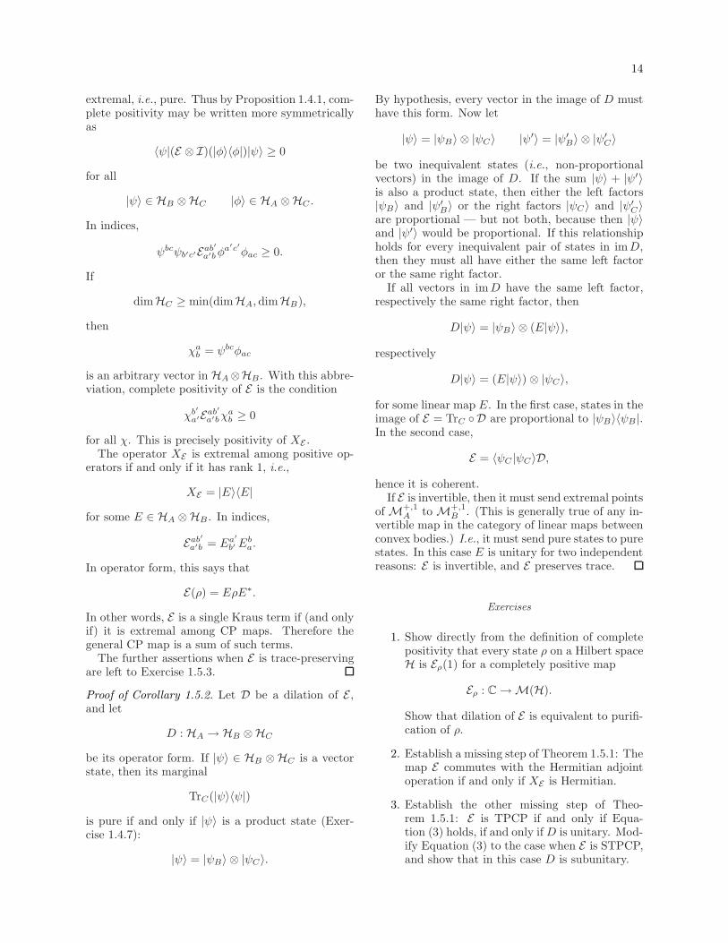
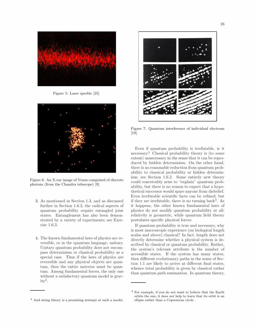
2. A variety of real experiments and demonstra-tions match the thought experiments of quan-tum probability. This includes the examples inthis article. For one, the two-slit “experiment”in Section 1.1 is a qualitatively correct modelof laser speckle (scattering interference) andholography (photographic interference). Laserspeckle is familiar as the twinkle in the dot of alaser pointer; see Figure 5. At the same time,light is composed of discrete, non-interactingphotons. This is an unavoidable aspect of low-intensity X-ray photography, as shown in Fig-ure 6.

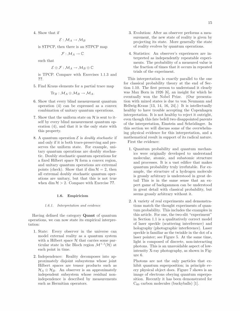
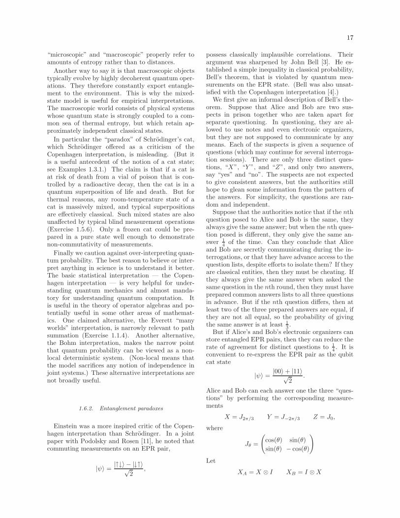
Photons are not the only particles that ex-hibit quantum superposition; in principle ev-ery physical object does. Figure 7 shows is animage of electrons obeying quantum superpo-sition. Recently it has been demonstrated forC60 carbon molecules (buckyballs) [1].

16

Figure 5: Laser speckle [25].

Figure 6: An X-ray image of Venus comprised of discretephotons (from the Chandra telescope) [9].

3. As mentioned in Section 1.3, and as discussedfurther in Section 1.6.2, the radical aspects ofquantum probability require entangled jointstates. Entanglement has also been demon-strated by a variety of experiments; see Exer-cise 1.6.3.

4. The known fundamental laws of physics are re-versible, or in the quantum language, unitary.Unitary quantum probability does not encom-pass determinism or classical probability as aspecial case. Thus if the laws of physics arereversible and any physical objects are quan-tum, then the entire universe must be quan-tum. Among fundamental forces, the only onewithout a satisfactory quantum model is grav-ity2.

2 And string theory is a promising attempt at such a model.

Figure 7: Quantum interference of individual electrons[19].

Even if quantum probability is irrefutable, is itnecessary? Classical probability theory is (to someextent) unnecessary in the sense that it can be repro-duced by hidden determinism. On the other hand,there is no reasonable reduction from quantum prob-ability to classical probability or hidden determin-ism; see Section 1.6.2. Some entirely new theorycould conceivably arise to “explain” quantum prob-ability, but there is no reason to expect that a hypo-thetical successor would spare anyone from disbelief.Even irrefutable scientific facts can be refined; butif they are irrefutable, there is no turning back3. Asit happens, the other known fundamental laws ofphysics do not modify quantum probability at all:relativity is geometric, while quantum field theorypostulates specific physical forces.

If quantum probability is true and necessary, whyis most macroscopic experience (on biological lengthscales and above) classical? In fact, length does notdirectly determine whether a physical system is de-scribed by classical or quantum probability. Rather,the system’s relevant attribute is the number ofaccessible states. If the system has many states,then different evolutionary paths in the sense of Sec-tion 1.1 are likely to arrive at different final states,whence total probability is given by classical ratherthan quantum path summation. In quantum theory,

3 For example, if you do not want to believe that the Earthorbits the sun, it does not help to learn that its orbit is anellipse rather than a Copernican circle.

17

“microscopic” and “macroscopic” properly refer toamounts of entropy rather than to distances.

Another way to say it is that macroscopic objectstypically evolve by highly decoherent quantum oper-ations. They therefore constantly export entangle-ment to the environment. This is why the mixed-state model is useful for empirical interpretations.The macroscopic world consists of physical systemswhose quantum state is strongly coupled to a com-mon sea of thermal entropy, but which retain ap-proximately independent classical states.

In particular the “paradox” of Schrodinger’s cat,which Schrodinger offered as a criticism of theCopenhagen interpretation, is misleading. (But itis a useful antecedent of the notion of a cat state;see Examples 1.3.1.) The claim is that if a cat isat risk of death from a vial of poison that is con-trolled by a radioactive decay, then the cat is in aquantum superposition of life and death. But forthermal reasons, any room-temperature state of acat is massively mixed, and typical superpositionsare effectively classical. Such mixed states are alsounaffected by typical blind measurement operations(Exercise 1.5.6). Only a frozen cat could be pre-pared in a pure state well enough to demonstratenon-commutativity of measurements.

Finally we caution against over-interpreting quan-tum probability. The best reason to believe or inter-pret anything in science is to understand it better.The basic statistical interpretation — the Copen-hagen interpretation — is very helpful for under-standing quantum mechanics and almost manda-tory for understanding quantum computation. Itis useful in the theory of operator algebras and po-tentially useful in some other areas of mathemat-ics. One claimed alternative, the Everett “manyworlds” interpretation, is narrowly relevant to pathsummation (Exercise 1.1.4). Another alternative,the Bohm interpretation, makes the narrow pointthat quantum probability can be viewed as a non-local deterministic system. (Non-local means thatthe model sacrifices any notion of independence injoint systems.) These alternative interpretations arenot broadly useful.

1.6.2. Entanglement paradoxes

Einstein was a more inspired critic of the Copen-hagen interpretation than Schrodinger. In a jointpaper with Podolsky and Rosen [11], he noted thatcommuting measurements on an EPR pair,

|ψ〉 =|↑↓〉 − |↓↑〉√

2,

possess classically implausible correlations. Theirargument was sharpened by John Bell [3]. He es-tablished a simple inequality in classical probability,Bell’s theorem, that is violated by quantum mea-surements on the EPR state. (Bell was also unsat-isfied with the Copenhagen interpretation [4].)

We first give an informal description of Bell’s the-orem. Suppose that Alice and Bob are two sus-pects in prison together who are taken apart forseparate questioning. In questioning, they are al-lowed to use notes and even electronic organizers,but they are not supposed to communicate by anymeans. Each of the suspects is given a sequence ofquestions (which may continue for several interroga-tion sessions). There are only three distinct ques-tions, “X”, “Y ”, and “Z”, and only two answers,say “yes” and “no”. The suspects are not expectedto give consistent answers, but the authorities stillhope to glean some information from the pattern ofthe answers. For simplicity, the questions are ran-dom and independent.

Suppose that the authorities notice that if the nthquestion posed to Alice and Bob is the same, theyalways give the same answer; but when the nth ques-tion posed is different, they only give the same an-swer 1

4 of the time. Can they conclude that Aliceand Bob are secretly communicating during the in-terrogations, or that they have advance access to thequestion lists, despite efforts to isolate them? If theyare classical entities, then they must be cheating. Ifthey always give the same answer when asked thesame question in the nth round, then they must haveprepared common answers lists to all three questionsin advance. But if the nth question differs, then atleast two of the three prepared answers are equal, ifthey are not all equal, so the probability of givingthe same answer is at least 1

3 .But if Alice’s and Bob’s electronic organizers can

store entangled EPR pairs, then they can reduce therate of agreement for distinct questions to 1

4 . It isconvenient to re-express the EPR pair as the qubitcat state

|ψ〉 =|00〉+ |11〉√

2.

Alice and Bob can each answer one the three “ques-tions” by performing the corresponding measure-ments

X = J2π/3 Y = J−2π/3 Z = J0,

where

Jθ =

(cos(θ) sin(θ)

sin(θ) − cos(θ)

)

Let

XA = X ⊗ I XB = I ⊗X

18

be the corresponding factor measurements for Aliceand Bob, and likewise for Y and Z. Then (Exer-cise 1.6.1):

1. Each of the six variables is an unbiased ±1-valued random variable.

2. The variables XA and XB (and likewise for Yand Z) agree with probability 1.

3. The variables XA and YB (and likewise theother pairs) agree with probability 1

4 .

(Note that each pair of questions converts an EPRpair to a product state; the EPR pair cannot bereused.) If the interrogators witness these classicallyimpossible correlations, they might be tempted toseize Alice’s and Bob’s electronic devices and try touse them to communicate with each other. But theywould not succeed, because no quantum operationon Alice’s qubits affects the marginal state on Bob’squbits, or vice-versa.

More formally, Bell’s theorem is an inequality con-cerning correlations of two-valued classical randomvariables which does not hold for quantum randomvariables:

Theorem 1.6.1 (Bell). If X, Y , and Z are threeclassical random variables taking values in {±1},then

E[XY ] + E[XZ] + E[Y Z] ≥ −1.

Proof. We would like to show, equivalently, that

E[XY +XZ + Y Z] ≥ −1.

It is easy to check that

XY +XZ + Y Z =

{3 if X = Y = Z

−1 otherwise.

Since the random variable XY +XZ+Y Z is alwaysat least −1, its expectation is at least −1.

A variant of the Bell-EPR paradox (with a dif-ferent set of classically impossible correlations) wasfamously demonstrated in an experiment by Aspectet al [2], and since then by others. In the experi-ment the two halves of Bell-state photon pairs wereinterrogated at almost simultaneously, so that therewas not enough time for a message to travel fromone photon to the other. These experiments shouldnot be taken as self-contained proof of that quan-tum probability is true, because they have possible“loopholes” that could allow the photons to com-municate. At the same time, there is no evidence

of any genuine interaction between the photons inthese demonstrations, much less non-quantum inter-actions that would present an illusion of quantumnon-interaction.

The original purpose of the Bell-EPR paradox wasthe simple conclusion that quantum operations donot admit a deterministic or classically random sim-ulation that preserves locality. In hindsight, it isa first step in the direction of quantum algorithms(Section ??) and especially quantum security (Sec-tion ??), since these can also be viewed as entan-glement paradoxes. The problem of communicationsecurity is for two parties (Alice and Bob) to shareinformation with some confidence that there is noeavesdropper (Eve). The shared information is ide-ally random, because it can then be used to maskarbitrary messages. In Bell’s protocol, the same ar-gument that Alice’s and Bob’s answers are classi-cally impossible also shows that there cannot be anEve who knows their answers in advance. Thus theshared answers are also shared secrets.

The relation to quantum algorithms is less for-mal. Intuitively, quantum algorithms exploit entan-glement as a kind of communication. For example,the result of Grover’s search algorithm (Section ??)can be described as a guessing game: If Alice thinksof a number from 1 to N and only responds “yes” or“no” depending one whether Bob guesses correctly,then Bob can guess it with O(

√N) guesses, provided

that he can guess in quantum superposition and Al-ice’s consideration of each guess is unitary. Grover’salgorithm is a classically impossible form of commu-nication afforded by quantum entanglement.

Exercises

1. Establish that Bell’s operators XA, YA, ZA,XB, YB, and ZB applied to a Bell state violateBell’s inequality.

2. The quantum violation of Bell’s theorem canbe called a “no hidden variables” theorem:Quantum operations cannot be simulated byhidden structure which is deterministic or clas-sically random. One rigorous (but possiblylimited) interpretation of this principle can bephrased as category theory: There does notexist a non-trivial linear tensor functor fromthe category Quant<inf to the category Prob.Prove this result using Bell’s theorem and mea-surements of EPR pairs.

3. The Aspect experiment employs the inequality

E[XAXB] + E[XAYB] + E[YAYB]− E[YAXB] ≤ 2

19

for ±1-valued classical random variables, dueto Clauser, Horne, Shimony, and Holt [8].(This avoids the assumption in Bell’s theoremthat when Alice and Bob perform the samemeasurement, they will agree with probabilityone.) Prove this inequality, and then find aviolation using the operators Jθ for four par-ticular values of θ.

1.7. Infinite systems

The immediate way to extend the finite-state the-ory to infinite quantum systems is to allow theHilbert space H to be infinite-dimensional (but usu-ally separable). Section 1.8 discusses a better andmore general extension due to von Neumann, butmuch can be learned from the this less creative ap-proach.

We can use various definitions from operator the-ory [? ] to adapt various objects such as states,random variables, and quantum operations to in-finite Hilbert spaces. Once these are defined, wecan define the category Quant to be the category ofHilbert spaces (both finite and infinite) with TPCPmaps as the morphisms or quantum operations.

First, a (normal) state ρ is defined as a positivesemi-definite trace-class operator with trace 1. Inother words, the Bloch region B+,1(H) is defined asthe trace 1 subspace of Bt(H), the algebra of trace-class operators. The spectral theorem for compactoperators implies that such a state ρ can be ex-pressed as:

ρ =∑

s∈S

ps|s〉〈s|

for some orthonormal basis S of H. Thus as in thefinite case, pure states (by definition the extremalelements of the Bloch region M+,1(H)) correspondto vector states (by definition unit vectors in H) upto a global phase.

A real-valued, bounded random variable X on His defined as a self-adjoint bounded operator. Thismatches the definition of states in that B(H), thealgebra of bounded operators, is the Banach spacedual of Bt(H). This duality means that for any stateρ and any bounded variable X , the trace Tr(ρX) iswell-defined as a finite real number. Thus we candefine the expectation

Eρ[X ]def= Tr(ρX)

as before. More generally, a state ρ and a real-valuedrandom variable X produce a probability measureon R, the distribution of X , by the spectral theoremfor bounded operators. This theorem expressesX as

an integral with respect to an operator-valued mea-sure µP whose value on any interval is a projectionthat commutes with X :

X =

∫

R

λdµP . (5)

If we pair the measure µP with the state ρ, the resultis the desired scalar-valued measure on R, indeed onthe spectrum of X .

A (projective) measurement X is again defined asa direct sum decomposition

H ∼=⊕

s∈S

Hs

for some outcome set S, which may now be infinite.Probabilities and conditional states have the sameformulas:

Pρ[X = s] = Tr(Psρ) ρ|X=s =PsρPs

P [X = s].

Not every real-valued random variable defines a mea-surement of this type. Rather, the spectral theoremsays that a Hermitian operator X has a point spec-trum and a continuous spectrum. Only the pointspectrum possesses eigenspaces, so X must have apure-point spectrum in order to define a measure-ment. However, there are various ways to approxi-mately measure a continuous-spectrum values of anoperator. The point spectrum is usually discrete,meaning that the eigenvalues are isolated, while thecontinuous spectrum usually consists of intervals,which in quantum mechanics are called bands. Butthere are other possibilities for both parts of thespectrum.

An unbounded random variable is defined as aself-adjoint unbounded operator, although such anoperator is an artifice in the sense that it is onlydefined on a dense subset of H. By definition it isa densely defined function whose graph is a closedvector subspace of H ⊕ H which is invariant underswitching the two summands. The definition is cho-sen so that self-adjoint operators satisfy the spectraltheorem. If X is a self-adjoint operator, then

U(t) = eitX

is a one-parameter group of unitary operators, andconversely every strongly continuous one-parametergroup of unitary operators defines a possibly un-bounded operator. Either the spectral theorem orthe unitary operator model could be taken as analternate definition of an unbounded self-adjoint op-erator.

Example 1.7.1. The function spaces L2(Rd), with1 ≤ d ≤ 3, are very common in quantum mechan-ics. Pure states are naturally referred to as wave or

20

amplitude functions. Technically they are half den-sities, meaning that the square norm of a wave func-tion is a probability density function with a volumeform factor. For example, the wave function

ψ(x) =e−x2/2

π1/4

√dx,

here written as a half density, is called a coherentstate onH = L2(R) (notwithstanding that elsewhereevery pure state is called coherent). It will appearlater as the ground state of the harmonic oscillator.

To give an example of a mixed state on L2(R), leta ≥ 1 and let

ρ(x, y) =1√πaea(x−y)2+a−1(x+y)2)/4

be a kernel (in the sense of integration, not nullspaces). The corresponding operator

ρ(f)(x) =

∫

R

ρ(x, y)f(y)dy

is trace-class with trace 1 and is called a quasifreestate; when a = 1 it is the coherent state.

Example 1.7.2. If f(x) is a continuous (or evenintegrable) function on R, then multiplication by f isan operator on H which is given the same name. Forexample, x is an unbounded, continuous-spectrumoperator whose distribution with respect to the purestate ψ(x) has the density function |ψ(x)|2. Anotherexample is the operator

p = −i ∂∂x

which has the same spectrum as x, namely all of Ras a continuous spectrum. They are both Gaussianrandom variables with respect to coherent and quasi-free states. We will see later that the operator

H =p2 + x2

2

has discrete spectrum Z≥0 + 12 . In the standard co-

herent state, H is definite with value 12 , while in a

standard quasi-free state, it has a discrete exponen-tial distribution.

Exercises

1.8. Operator algebras

Following von Neumann, we can represent a quan-tum object not as a Hilbert space H, but as an ab-stract algebra A whose elements can be called “op-erators”. Such an operator algebra should satisfy

suitable axioms so that we can define states, randomvariables, and quantum operations. Von Neumanndefined two types of algebras for this purpose, C∗-algebras and W ∗-algebras; the latter are now calledvon Neumann algebras. Von Neumann algebras areactually just C∗-algebras with a stronger topologicalclosure property.

The algebrasM(H) of all bounded operators on aHilbert spaces H are one class of von Neumann alge-bras that happen to contain all von Neumann alge-bras as subalgebras. But considering only M(H) isa very restricted view of the theory of operator alge-bras, just as considering only symmetric groups is avery restricted view of finite group theory. Quantumphysics has also drifted towards considering specificalgebras of operators, although not usually with vonNeumann’s axioms.

A C∗-algebra A is, first, a complex vector spacewith an associative and bilinear multiplication law.It also has an abstract anti-linear, product-reversingadjoint operation denoted “∗”:

(X + Y )∗ = X∗ + Y ∗ (λXY )∗ = λY ∗X∗.

Finally A is also a Banach space a norm || · || thatsatisfies the relation

||X∗X || = ||X ||2.

This last axiom, the “C∗ axiom” is coy and has manyconsequences for the structure of A. Among otherthings, it means that the norm || · || is completelydetermined by the algebra structure of A and that

||X∗|| = ||X ||.

IntuitivelyA consists of bounded operators and ||X ||behaves as the spectral radius of X . For simplicitywe will assume that every C∗-algebra A has a unit,even though non-unital C∗-algebras are also an in-teresting class.

Possessing a unit is traditionally an optional ax-iom for C∗-algebras; we will assume it for simplicity.

Theorem 1.8.1 (Gelfand,Naimark). If A is a (uni-tal) commutative C∗-algebra, then it is isomorphic toan algebra of continuous functions C(A) on a com-pact Hausdorff topological space A.

By Theorem 1.8.1, and since C(A) is a C∗-algebrafor every compact Hausdorff space A, a C∗-algebracan be thought of as a “non-commutative topolog-ical space”. In particular if A is a finite set, thenC(A) = CA is exactly the model of finite probabil-ity described in Section 1.10 — its set of normalizedstates is ∆A.

Theorem 1.8.1 also implies that if X ∈ Asa (theself-adjoint subspace of A) and f : R → R is a con-tinuous function, then there is a well-defined element

21

f(X) ∈ Asa (Exercise ??). For example, sinX and|X | are well-defined. We will need a slight gener-alization of this principle: An element X ∈ Asa ispositive, or X ≥ 0, if X = Y ∗Y for some Y . Iff : R≥0 → R is continuous and X ≥ 0, then f(X) iswell-defined; if f ≥ 0 as a function, then f(X) ≥ 0.

A representation of a C∗-algebra A is a homomor-phism from A to the C∗-algebra B(H) of boundedoperators on a Hilbert space. (A homomorphism be-tween two C∗-algebras is a linear map that respectsmultiplication, ∗, and is continuous with respect tothe Banach norm.) Crucially, the algebra B(H) hasother topologies besides the one coming from its Ba-nach norm, namely the strong and weak operatortopologies. If M is a C∗-algebra which is closedwith respect to the weak operator topology in somefaithful representationH, thenM is a von Neumannalgebra.

Theorem 1.8.2. If M is a commutative von Neu-mann algebra, then it is isomorphic to the algebraL∞(M) for some σ-field M .

By Theorem 1.8.2, and since L∞(M) is a von Neu-mann algebra for many natural σ-fields M , a vonNeumann algebra M can be thought of as a “non-commutative measure space”.

Theorem 1.8.2 also implies that if X ∈ Msa (theself-adjoint subspace of A) and f : R→ R is a mea-surable function, then there is a well-defined elementf(X) ∈Msa. This closure property is called “func-tional calculus”.

The traditional definition of von Neumann alge-bra via a faithful action on a Hilbert space H iscontrary to our intention of emphasizing operatorsover vectors. Happily there are other characteriza-tions of von Neumann algebras within the class ofC∗-algebras:

Theorem 1.8.3 (???). A C∗ algebra M is a vonNeumann algebra if and only if it has a pre-dual#M as a Banach space. The pre-dual, if it exists,is unique up to isometry.

In particular, the algebra B(H) of bounded opera-tors on a Hilbert space H is a von Neumann algebrawith pre-dual Bt(H). Theorem 1.8.3 interplays withthe general fact that every Banach space B embedsisometrically in its second dual B##. Thus the pre-dual #M can be viewed as subspace of the dualM#.Also, by a construction of ???, if A is a C∗-algebra,its second dual A## has the natural structure of avon Neumann algebra, the universal enveloping vonNeumann algebra of A.

If A and B are two C∗ algebras, there is a naturaltensor product C∗-algebraA⊗B which is a topologi-cal completion of the algebraic tensor product. IfM

and N are von Neumann algebras, there a von Neu-mann algebraM⊗N which is a further topologicalcompletion than the C∗-algebra completion.

After accepting these preliminaries (perhaps onfaith), we can proceed to define the basic structuresof quantum probability. A C∗-algebra A or a vonNeumann algebra M can be assigned. The algebrais termed its algebra of observables, because the self-adjoint elements (Asa orMsa) will be interpreted asreal-valued random variables. If A is a C∗-algebra,a state is a dual vector ρ ∈ A# which is positive,meaning that

X ≥ 0 =⇒ ρ(X) ≥ 0.

The state ρ is normalized if

ρ(I) = 1.

Previously we took ρ to be an operator rather thana dual vector; this is not really different if we define

ρ(X) = Tr(ρX).

In particular we can call ρ(I) the “trace” of ρ.A state ρ on a von Neumann algebraM is normal

if it lies in the pre-dual #M. The commutative caseillustrates the reason to take states from the dual of aC∗-algebra but from the pre-dual of a von Neumannalgebra. If A = C(A), then by the ??? theorem,states are equivalent to finite Borel measures on A.If M = L∞(M), then general states are equivalentto finitely additive, finite measures on M ; normalstates are equivalent to countably additive measuresand are hence more empirical. Note also that thestates of the C∗-algebra A are the normal states ofthe von Neumann algebra A##.

A pair (M, ρ) consisting of a von Neumann al-gebra M and a normalized, normal state ρ isalso called a quantum probability space or a non-commutative probability space. Each random vari-ableX ∈ Msa has a well-defined spectrum SpecX ⊂R (which depends crucially on the structure ofM),and each state ρ induces a probability distributionon SpecX . If M ⊆ B(H) is defined as an alge-bra of operators on a Hilbert space, one way toconstruct the spectrum and distribution of X is byEquation (5). The point is that #M is a quotient ofBt(H), and we can use any lift of ρ to a trace-classoperator on H.

As usual, ifA and B are Alice’s and Bob’s algebrasof observables, their joint algebra of observables isA⊗ B.

If A and B are C∗-algebras, then a linear map

E : B → Ais positive if it takes positive elements of A to posi-tive elements of B; it is completely positive if

E ⊗ I : B ⊗ C → A⊗ C

22

is positive for every C∗-algebra C; and it is unital if

E(I) = I.

If M and N are von Neumann algebras, a linearmap

E : N →M

is normal if it has a pre-transpose

#E : #M→ #N .

In general E is unital if and only if the pre-transpose#E (or the transpose E#) is trace-preserving. Thecategory vN is defined as the category of pre-dualsof von Neumann algebras with TPCP maps as itsmorphisms. Equivalently it is the category of vonNeumann algebras with normal UCP (unital andCP) maps as contravariant morphisms (Exercise ??).The category vN is the most satisfactory model ofinfinite quantum probability, and its morphisms canbe called quantum operations. An interesting also-ran is the category C∗ of C∗ algebras with arbitraryUCP maps as contravariant morphisms. AlthoughvN can be viewed as a subcategory of C∗, C∗ canalso be viewed as a subcategory of vN, by takingeach C∗-algebra A to its enveloping algebra A##.

1.9. Classical and quantum coexistence

Because the category vN includes commutativealgebras, which are the corresponding models of clas-sical probability, they can model coexistence of clas-sical and quantum objects and interactions betweenthem. We can then use these categories to studymeasurements of quantum systems by classical ob-servers, and classical behavior of quantum systems.(As discussed in Section 1.6.2, the converse of thelatter is impossible.)

As a first case, suppose that Alice is classical andfinite, so that her von Neumann algebra is

A = CA

for some finite set A. Suppose that Bob has someother von Neumann algebra B. Then we can ax-iomatically define a destructive measurement to bean arbitrary quantum operation

E : #B → #A.

Then (Exercise ??) the general form of P is

E(ρ) =⊕

a∈A

ρ(Ea),

where each Ea ≥ 0 and

∑

a∈A

Ea = I.

This structure is also known concretely as a positive,operator-valued measure, or POVM, because it is aprobability measure on A that takes values in thepositive cone B+ rather than in the real numbers.

We can construct a sensible conditional state on Bin the same setting. It would be given by a quantumoperation

F : #B → #B ⊗ #A

such that the composition TrB ◦ F (in which Aliceapplies F and then destroys Bob) is a POVM

E : #B → #A.

We further suppose that F is initial among all suchfactors of E , in the sense that Bob retains as much in-formation as possible about his previous state. Then(Exercise ??) one form for F is

F =⊕

a∈A

[a]⊗ ρ√

Ea ,

where in general the state ρX is defined as

ρX(Y ) = ρ(X∗Y X);

also if X ≥ 0,√X is its unique positive square root.

In light of this possible structure for F , the condi-tional state of the POVM E applied to ρ with out-come a is

ρ|E=a = ρ√

Ea .

Finally the POVM E has mutually exclusive out-comes if and only if its non-destructive lift F is aprojection, i.e., F2 = F . In this case (Exercise ??)the Eas are projections such that

EaEa′ = 0

when a 6= a′. Thus the projective measurements de-fined in Sections ?? and ?? are exactly those POVMswith mutually exclusive outcomes.

The above discussion can be extended to the casewhere Alice is classical but infinite. In this case hervon Neumann algebra is L∞(A) for some σ-field A,and a POVM is a measure on A that takes values inB+. This structure is closely related to a normalizedmeasure on B+ itself.

We turn to a result from the theory of operatoralgebras that shows how decoherence can reduce aquantum object to a classical one. Suppose that A

23

is Alice’s algebra of observables and that she evolvesaccording to a quantum operation

P : A → Ain a unit period of time. Very often we can supposethat P is an idempotent, i.e., P2 = P (Exercise ??).Intuitively this means that Alice stabilizes in a shortperiod of time and, once stable, her temporal evolu-tion does not further affect her state.

Theorem 1.9.1 (Choi-Effros). If A is a C∗-algebraand P is an SUCP idempotent on A, then the imageof P is a C∗-algebra B with a modified product

X ◦ Y = P(XY ).

Theorem 1.9.1 says that if Alice’s evolution is anidempotent P , then she can be modelled by a smallereffective C∗-algebra B. In particular, B can be com-mutative even whenA is not. The algebra B is a vec-tor subspace of A, but not in general a subalgebra.Rather, the modified product defined by Choi andEffros matches the process of applying P betweenexternal interactions with Alice. Note also that if Ais a von Neumann algebra and if P is normal, thenB is also a von Neumann algebra.

Example 1.9.1. The blind projective measurementoperation P defined in Equation (4) is an idempo-tent. In this case imP is closed under multiplicationand is the algebra

⊕

s∈S

M(Hs).

Finally, the classification of finite-dimensional C∗-algebras, or von Neumann algebras, also fits thetheme of classical and quantum coexistence. Saythat a ∗-algebra A is positive if

X∗X = 0 =⇒ X = 0.

If A is positive and finite-dimensional, then it is au-tomatically a C∗-algebra, indeed a von Neumann al-gebra. This can be seen from the following classifi-cation theorem.

Theorem 1.9.2 (Artin-Schreier). If A a positive,finite-dimensional ∗-algebra, then it is a direct sumof matrix algebras:

A ∼=n⊕

k=1

Mλk

for some integers

λ1 ≥ λ2 ≥ · · · ≥ λn.

The vector (λ1, λ2, . . . , λn) in Theorem 1.9.2 canbe called the shape of the algebra A.

Examples 1.9.2. A joint system consisting of a fi-nite classical Alice with algebra Cn and a finite quan-tum Bob with algebraMk has the rectangular shape(k, k, . . . , k). For example, Bob could be a quantumcomputer with qubit memory and Alice could be aclassical controllers with classical bit memory. Thefirst finite quantum system which is not of this formis the hybrid trit M2 ⊕ C. The author [? ] hasanalyzed the storage properties of finite quantumsystems such as the hybrid trit.

Exercises

1.10. Appendix: A classical review

Consider a classical probabilistic system with a fi-nite set A of configurations. The general probabilitydistribution or measure µ on A can be written in theform

µ =∑

a∈A

pa[a],

where each probability pa ≥ 0 and

∑

a∈A

pa = 1.

The symbol [a] represents both the configuration aand the probabilistic state in which a is certain.(This state is also called an atom or a Kroneckerdelta function.) The set of all normalized statesforms a simplex ∆A whose vertices are the set A.These simplices are the objects of a reasonable ifslightly non-standard definition of finite, classicalprobability theory. The other elements of this defi-nition are as follows.

An event is a subset E ⊆ A. A state µ assigns aprobability to E between 0 and 1 by the formula

P [E] = Pµ[E] =∑

a∈A

pa.

If P [E] > 0, then E and µ induce a conditional stateon E given by the formula

µ|E =1

P [E]

∑

a∈E

pa [a].

A random variable or measurement is a functionX : A → B for some set B. It is interpreted asa partition of A into disjoint events: the equationX = b, as an event, is the set of all a such that

24

X(a) = b. If X takes values in R or C, then it alsohas an expectation, defined as

E[X ] =∑

a

paX(a).

If A and B are two finite configuration sets, thena function

M : ∆A → ∆B

is a stochastic map (or a Markov map) if it comesfrom a linear map

M : RA → RB.

The linearity ofM is the classical superposition prin-ciple. Another way to describe a stochastic map isto start with a linear map M and impose the posi-tivity condition M(∆A) ⊆ ∆B. If M is viewed as amatrix, the positivity condition says that the entriesof M are non-negative and each column sums to 1.In this case M is called a stochastic matrix. Stochas-tic maps are the natural empirical class of maps inprobability theory.

A non-negative vector µ in RA is a subnormalizedstate if the total probability is at most 1, and a linearmap

M : RA → RB

that preserves subnormalized states is called sub-stochastic. A substochastic map is also called anextinction process. It can be converted to a stochas-tic map by adding an extinction state to the targetset B.

If A and B are the configuration sets of two proba-bilistic systems, then the two systems together havea joint configuration set A × B. The joint simplex∆A×B lies in a tensor product:

∆A×B ⊂ R(A×B) = RA ⊗ RB.

A joint state µ ∈ ∆A×B is independent or a productstate if it factors as a tensor product:

µ = µA ⊗ µB.

More typically µ does not have this form, in whichcase it is correlated. A stochastic map that affectsonly one of A and B has the form M ⊗ I or I ⊗M ;likewise an event that depends on only one of A orB has the form E ×B or A× E. Whether or not µis independent, it induces states on A and B calledmarginals. They are defined as:

µA =∑

a∈A

(∑

b∈B

p(a,b)

)[a] µB =

∑

b∈B

(∑

a∈A

p(a,b)

)[b].

Evidently, if µ is a product, then it is the product ofits marginals.

Example 1.10.1. Two fair dice are rolled. If wetake the dice as subsystems A and B with a jointstate, then A = B = {1, . . . , 6} and the state µ isthe uniform state

µ =1

36

∑

1≤s,t≤6

[(s, t)].

The event of rolling 7 is the set E = {(s, t)|s+t = 7}.The chance of E is P [E] = 1

6 . The state µ is anindependent state, but the conditional state µ|E iscorrelated. A protocol such as “if you rolled 7, pickone die at random and roll it again” is modelled bya stochastic map.

The rules of classical probability theory are thebasis of a (Bayesian) statistician’s model of ordinaryhuman experience, as well as most scientific experi-ments, according to the following interpretation:

1. State: Each observer can model external re-ality as a measure space, such as a finite setA, that carries has probability distribution ateach point in time.

2. Independence: Reality decomposes into ap-proximately disjoint subsystems modelled byCartesian products of measure spaces. An ob-server is an approximately independent sub-system whose residual non-independence is de-scribed by witnessed information.

3. Evolution: After an observer witnesses anevent, the new state of reality is given byconditional expectation. More generally thestate of reality evolves by stochastic and sub-stochastic maps.

4. Statistics: An observer’s experiences areviewed as independently repeatable experi-ments. The probability of an event is the frac-tion of times that it occurs in repeated trialsof the experiment.

These rules can be accepted in one of two ways:(1) they hold empirically; (2) they can be mimickedby deterministic systems with hidden information.The first reason, but not the second, applies to thequantum analogue of these rules.

Exercises

1.11. Appendix: Categories and tensors

Much of the presence of category theory in math-ematics is in the spirit of Moliere: You can usecategories without knowing it. In many areas of

25

mathematics there is a distinguished class of objects(e.g., sets, groups, topological spaces, vector spaces)and a distinguished class of functions between them(e.g.all functions, group homomorphisms, continu-ous functions, linear maps). In some cases two ob-jects are related by a transformation which isn’tstrictly a function but behaves a lot like one; the his-torically important example was a function betweentwo topological spaces considered up to homotopy.

A category C is a possibly abstract class of set-like objects and a class of function-like relations, ormorphisms. Every morphism f has a domain A anda target B (both of them objects in C) and is thendenoted

f : A→ B.

There is a partial composition law: If the target off is the same object as the domain of g, or

f : A→ B g : B → C,

then there is a composition

f ◦ g : A→ C.

The composition law for C is required to be asso-ciated, and for every object A there should be anidentity morphism

i : A→ A

which satisfies the obvious identity axiom with re-spect to composition. These axioms are not all thatrestrictive and there are a wide variety of differentkinds of categories.

Examples 1.11.1. The category of sets, with allfunctions as the morphisms, is called Set. The cate-gory of vector spaces over a field F, with linear trans-formations as the morphisms, can be called VectF.The category of topological spaces with continuousfunctions as the morphisms is called Top.

Two different categories can have the same objectsbut different morphisms. For example, the obejctsof the category iSet are sets, but the morphisms arejust the injective functions.

As an example of a more abstract category, if G isa group, it yields a category with one object whosemorphisms are the elements of G.

A tensor category is a category with a multiplica-tion law, denoted “⊗” and called a “tensor product”,for both objects and morphisms. The multiplicationlaw should be associative: A⊗(B⊗C) should be thesame object as (A⊗B)⊗C4. The axioms for taking

4 There is a distinction between a strict tensor category, in

tensor products of morphisms is more complicatedbecause the axioms include compatibility relationsbetween the operations of composing and tensoringmorphisms. The tensor categories of interest in thisarticle are all symmetric, meaning that “⊗” is com-mutative as well as associative, both for objects andmorphisms.

The most important example of a tensor categoryis Vect, the category of vector spaces.

which A⊗ (B ⊗ C) and (A⊗ B)⊗ C are exactly the sameobject, and a lax tensor category, in which they are iso-morphic and the isomorphisms are meta-associative; thismeta-associativity is called “coherence”. We don’t have toworry about lax tensor categories here, but note that theyarise in physics in the guise of spin calculus; the main co-herence axiom is known as the Biedenharn-Elliott identity.

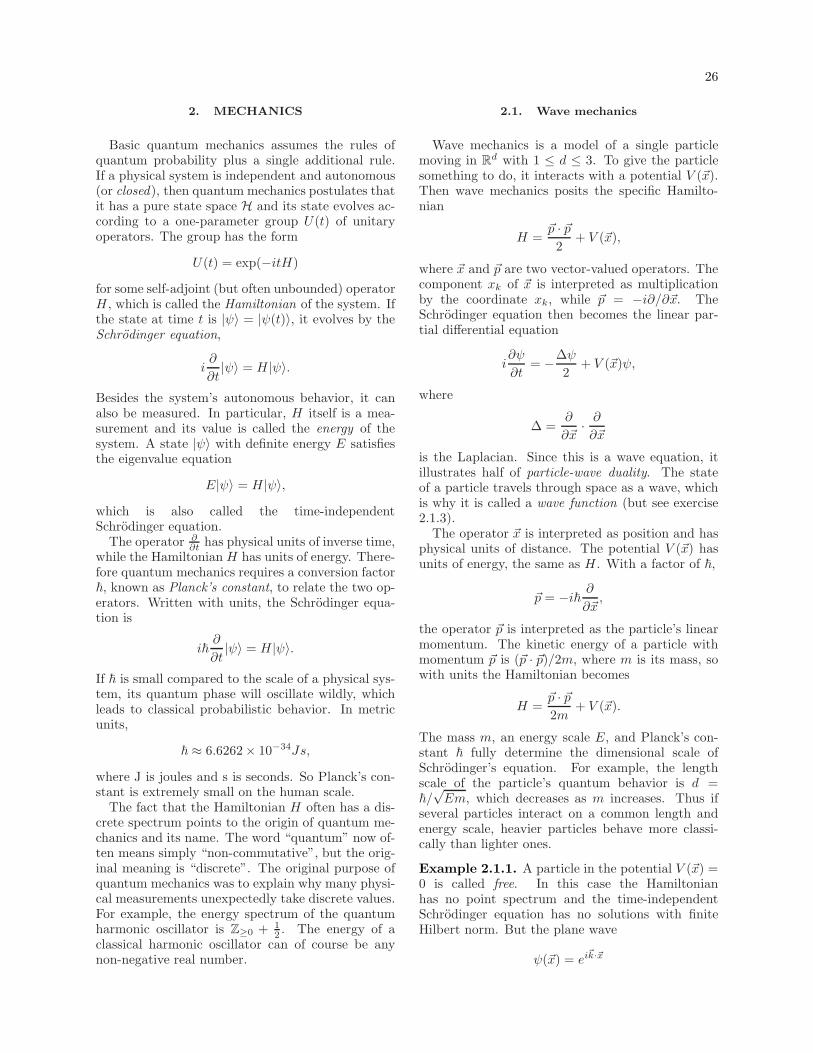
26

2. MECHANICS

Basic quantum mechanics assumes the rules ofquantum probability plus a single additional rule.If a physical system is independent and autonomous(or closed), then quantum mechanics postulates thatit has a pure state space H and its state evolves ac-cording to a one-parameter group U(t) of unitaryoperators. The group has the form

U(t) = exp(−itH)

for some self-adjoint (but often unbounded) operatorH , which is called the Hamiltonian of the system. Ifthe state at time t is |ψ〉 = |ψ(t)〉, it evolves by theSchrodinger equation,

i∂

∂t|ψ〉 = H |ψ〉.

Besides the system’s autonomous behavior, it canalso be measured. In particular, H itself is a mea-surement and its value is called the energy of thesystem. A state |ψ〉 with definite energy E satisfiesthe eigenvalue equation

E|ψ〉 = H |ψ〉,

which is also called the time-independentSchrodinger equation.

The operator ∂∂t has physical units of inverse time,

while the Hamiltonian H has units of energy. There-fore quantum mechanics requires a conversion factor~, known as Planck’s constant, to relate the two op-erators. Written with units, the Schrodinger equa-tion is

i~∂

∂t|ψ〉 = H |ψ〉.

If ~ is small compared to the scale of a physical sys-tem, its quantum phase will oscillate wildly, whichleads to classical probabilistic behavior. In metricunits,

~ ≈ 6.6262× 10−34Js,

where J is joules and s is seconds. So Planck’s con-stant is extremely small on the human scale.

The fact that the Hamiltonian H often has a dis-crete spectrum points to the origin of quantum me-chanics and its name. The word “quantum” now of-ten means simply “non-commutative”, but the orig-inal meaning is “discrete”. The original purpose ofquantum mechanics was to explain why many physi-cal measurements unexpectedly take discrete values.For example, the energy spectrum of the quantumharmonic oscillator is Z≥0 + 1

2 . The energy of aclassical harmonic oscillator can of course be anynon-negative real number.

2.1. Wave mechanics

Wave mechanics is a model of a single particlemoving in Rd with 1 ≤ d ≤ 3. To give the particlesomething to do, it interacts with a potential V (~x).Then wave mechanics posits the specific Hamilto-nian

H =~p · ~p

2+ V (~x),

where ~x and ~p are two vector-valued operators. Thecomponent xk of ~x is interpreted as multiplicationby the coordinate xk, while ~p = −i∂/∂~x. TheSchrodinger equation then becomes the linear par-tial differential equation

i∂ψ

∂t= −∆ψ

2+ V (~x)ψ,

where

∆ =∂

∂~x· ∂∂~x

is the Laplacian. Since this is a wave equation, itillustrates half of particle-wave duality. The stateof a particle travels through space as a wave, whichis why it is called a wave function (but see exercise2.1.3).

The operator ~x is interpreted as position and hasphysical units of distance. The potential V (~x) hasunits of energy, the same as H . With a factor of ~,

~p = −i~ ∂

∂~x,

the operator ~p is interpreted as the particle’s linearmomentum. The kinetic energy of a particle withmomentum ~p is (~p · ~p)/2m, where m is its mass, sowith units the Hamiltonian becomes

H =~p · ~p2m

+ V (~x).

The mass m, an energy scale E, and Planck’s con-stant ~ fully determine the dimensional scale ofSchrodinger’s equation. For example, the lengthscale of the particle’s quantum behavior is d =~/√Em, which decreases as m increases. Thus if

several particles interact on a common length andenergy scale, heavier particles behave more classi-cally than lighter ones.

Example 2.1.1. A particle in the potential V (~x) =0 is called free. In this case the Hamiltonianhas no point spectrum and the time-independentSchrodinger equation has no solutions with finiteHilbert norm. But the plane wave

ψ(~x) = ei~k·~x

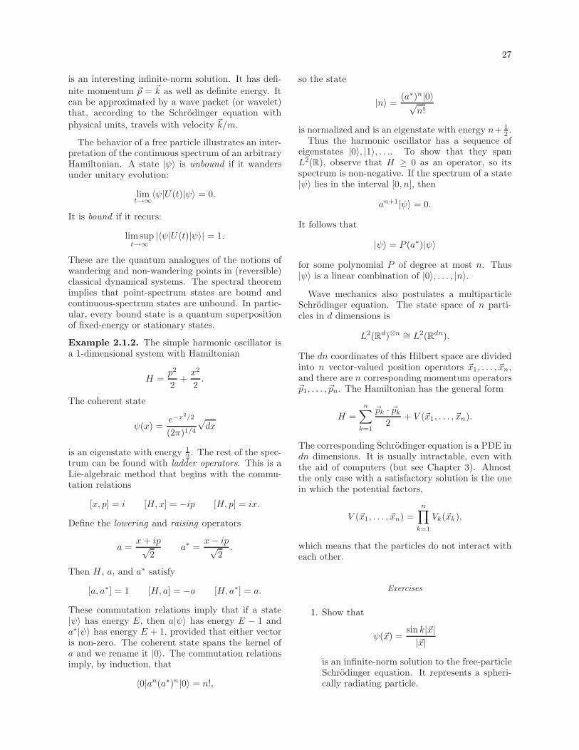
27

is an interesting infinite-norm solution. It has defi-

nite momentum ~p = ~k as well as definite energy. Itcan be approximated by a wave packet (or wavelet)that, according to the Schrodinger equation with

physical units, travels with velocity ~k/m.

The behavior of a free particle illustrates an inter-pretation of the continuous spectrum of an arbitraryHamiltonian. A state |ψ〉 is unbound if it wandersunder unitary evolution:

limt→∞〈ψ|U(t)|ψ〉 = 0.

It is bound if it recurs:

lim supt→∞

|〈ψ|U(t)|ψ〉| = 1.

These are the quantum analogues of the notions ofwandering and non-wandering points in (reversible)classical dynamical systems. The spectral theoremimplies that point-spectrum states are bound andcontinuous-spectrum states are unbound. In partic-ular, every bound state is a quantum superpositionof fixed-energy or stationary states.

Example 2.1.2. The simple harmonic oscillator isa 1-dimensional system with Hamiltonian

H =p2

2+x2

2.

The coherent state

ψ(x) =e−x2/2

(2π)1/4

√dx

is an eigenstate with energy 12 . The rest of the spec-

trum can be found with ladder operators. This is aLie-algebraic method that begins with the commu-tation relations

[x, p] = i [H,x] = −ip [H, p] = ix.

Define the lowering and raising operators

a =x+ ip√

2a∗ =

x− ip√2.

Then H , a, and a∗ satisfy

[a, a∗] = 1 [H, a] = −a [H, a∗] = a.

These commutation relations imply that if a state|ψ〉 has energy E, then a|ψ〉 has energy E − 1 anda∗|ψ〉 has energy E + 1, provided that either vectoris non-zero. The coherent state spans the kernel ofa and we rename it |0〉. The commutation relationsimply, by induction, that

〈0|an(a∗)n|0〉 = n!,

so the state

|n〉 =(a∗)n|0〉√

n!

is normalized and is an eigenstate with energy n+ 12 .

Thus the harmonic oscillator has a sequence ofeigenstates |0〉, |1〉, . . .. To show that they spanL2(R), observe that H ≥ 0 as an operator, so itsspectrum is non-negative. If the spectrum of a state|ψ〉 lies in the interval [0, n], then

an+1|ψ〉 = 0.

It follows that

|ψ〉 = P (a∗)|ψ〉

for some polynomial P of degree at most n. Thus|ψ〉 is a linear combination of |0〉, . . . , |n〉.

Wave mechanics also postulates a multiparticleSchrodinger equation. The state space of n parti-cles in d dimensions is

L2(Rd)⊗n ∼= L2(Rdn).

The dn coordinates of this Hilbert space are dividedinto n vector-valued position operators ~x1, . . . , ~xn,and there are n corresponding momentum operators~p1, . . . , ~pn. The Hamiltonian has the general form

H =n∑

k=1

~pk · ~pk

2+ V (~x1, . . . , ~xn).

The corresponding Schrodinger equation is a PDE indn dimensions. It is usually intractable, even withthe aid of computers (but see Chapter 3). Almostthe only case with a satisfactory solution is the onein which the potential factors,

V (~x1, . . . , ~xn) =n∏

k=1

Vk(~xk),

which means that the particles do not interact witheach other.

Exercises

1. Show that

ψ(~x) =sink|~x||~x|

is an infinite-norm solution to the free-particleSchrodinger equation. It represents a spheri-cally radiating particle.

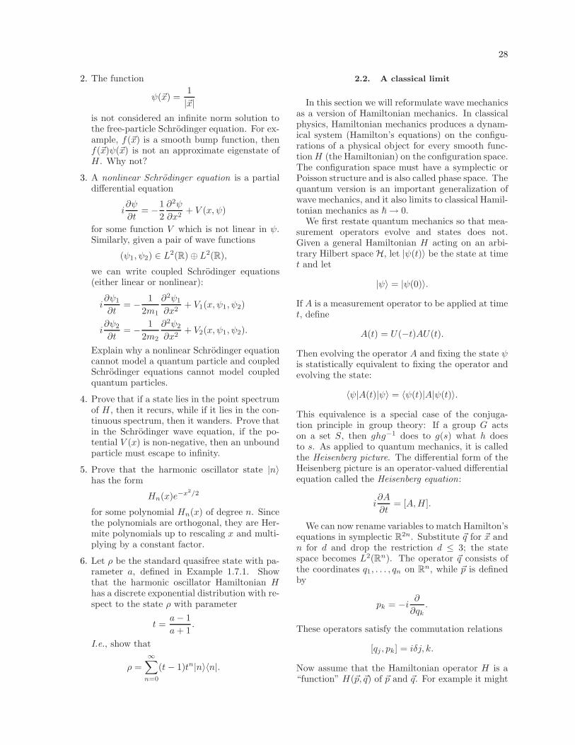
28

2. The function

ψ(~x) =1

|~x|is not considered an infinite norm solution tothe free-particle Schrodinger equation. For ex-ample, f(~x) is a smooth bump function, thenf(~x)ψ(~x) is not an approximate eigenstate ofH . Why not?

3. A nonlinear Schrodinger equation is a partialdifferential equation

i∂ψ

∂t= −1

2

∂2ψ

∂x2+ V (x, ψ)

for some function V which is not linear in ψ.Similarly, given a pair of wave functions

(ψ1, ψ2) ∈ L2(R)⊕ L2(R),

we can write coupled Schrodinger equations(either linear or nonlinear):

i∂ψ1

∂t= − 1

2m1

∂2ψ1

∂x2+ V1(x, ψ1, ψ2)

i∂ψ2

∂t= − 1

2m2

∂2ψ2

∂x2+ V2(x, ψ1, ψ2).

Explain why a nonlinear Schrodinger equationcannot model a quantum particle and coupledSchrodinger equations cannot model coupledquantum particles.

4. Prove that if a state lies in the point spectrumof H , then it recurs, while if it lies in the con-tinuous spectrum, then it wanders. Prove thatin the Schrodinger wave equation, if the po-tential V (x) is non-negative, then an unboundparticle must escape to infinity.

5. Prove that the harmonic oscillator state |n〉has the form

Hn(x)e−x2/2

for some polynomial Hn(x) of degree n. Sincethe polynomials are orthogonal, they are Her-mite polynomials up to rescaling x and multi-plying by a constant factor.

6. Let ρ be the standard quasifree state with pa-rameter a, defined in Example 1.7.1. Showthat the harmonic oscillator Hamiltonian Hhas a discrete exponential distribution with re-spect to the state ρ with parameter

t =a− 1

a+ 1.

I.e., show that

ρ =

∞∑

n=0

(t− 1)tn|n〉〈n|.

2.2. A classical limit

In this section we will reformulate wave mechanicsas a version of Hamiltonian mechanics. In classicalphysics, Hamiltonian mechanics produces a dynam-ical system (Hamilton’s equations) on the configu-rations of a physical object for every smooth func-tionH (the Hamiltonian) on the configuration space.The configuration space must have a symplectic orPoisson structure and is also called phase space. Thequantum version is an important generalization ofwave mechanics, and it also limits to classical Hamil-tonian mechanics as ~→ 0.

We first restate quantum mechanics so that mea-surement operators evolve and states does not.Given a general Hamiltonian H acting on an arbi-trary Hilbert space H, let |ψ(t)〉 be the state at timet and let

|ψ〉 = |ψ(0)〉.

If A is a measurement operator to be applied at timet, define

A(t) = U(−t)AU(t).

Then evolving the operator A and fixing the state ψis statistically equivalent to fixing the operator andevolving the state:

〈ψ|A(t)|ψ〉 = 〈ψ(t)|A|ψ(t)〉.

This equivalence is a special case of the conjuga-tion principle in group theory: If a group G actson a set S, then ghg−1 does to g(s) what h doesto s. As applied to quantum mechanics, it is calledthe Heisenberg picture. The differential form of theHeisenberg picture is an operator-valued differentialequation called the Heisenberg equation:

i∂A

∂t= [A,H ].

We can now rename variables to match Hamilton’sequations in symplectic R2n. Substitute ~q for ~x andn for d and drop the restriction d ≤ 3; the statespace becomes L2(Rn). The operator ~q consists ofthe coordinates q1, . . . , qn on Rn, while ~p is definedby

pk = −i ∂∂qk

.

These operators satisfy the commutation relations

[qj , pk] = iδj, k.

Now assume that the Hamiltonian operator H is a“function” H(~p, ~q) of ~p and ~q. For example it might

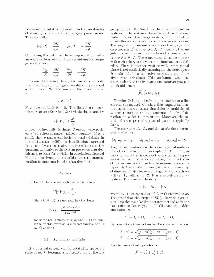
29

be a non-commutative polynomial in the coordinatesof ~p and ~q or a suitably convergent power series.Then formally

[qk, H ] = i∂H

∂pk[pk, H ] = −i ∂H

∂qk.

Combining this with the Heisenberg equation yieldsan operator form of Hamilton’s equations for conju-gate variables:

∂qk∂t

=∂H

∂pk

∂pk

∂t= −∂H

∂qk.

To see the classical limit, assume for simplicitythat n = 1 and the conjugate variables are just p andq. In units of Planck’s constant, their commutatoris

[q, p] = i~.

Now take the limit ~ → 0. The Heisenberg uncer-tainty relation (Exercise 1.2.8) yields the inequality

V [q]V [p] ≥ ~2

4.

In fact the inequality is sharp: Gaussian wave pack-ets (i.e., coherent states) achieve equality. If ~ issmall, then p and q can both be nearly definite inthe initial state |ψ(0)〉. A Hamiltonian expressedin terms of p and q is also nearly definite and thequantum dynamics of the system preserves near def-initeness at least for a while. In conclusion, classicalHamiltonian dynamics is a valid short-term approx-imation to quantum Hamiltonian dynamics.

Exercises

1. Let |ψ〉 be a state with respect to which

V [q]V [p] =~2

4.

Show that |ψ〉 is pure and has the form

ψ(x) =ea(x−b+ic)2/2

(πa)1/4

for some real constants a, b, and c. (The con-verse of this exercise is also worthwhile and ismuch easier.)

2.3. Symmetry and spin

If a physical system can be rotated in space, itsstate space H becomes a representation of the Lie

group SO(3). By Noether’s theorem for quantumsystems, if the system’s Hamiltonian H is invariantunder rotation, the Lie generators, if multiplied byi, are Hermitian operators with conserved values.The angular momentum operators in the x, y, and zdirections in R3 are written Jx, Jy, and Jz ; the an-gular momentum in the direction of a general unit

vector ~v is ~v · ~J . These operators do not commutewith each other, so they are not simultaneously def-inite. There is another twist as well. Since globalphase is not statistically meaningful, the state spaceH might only be a projective representation of anygiven symmetry group. This can happen with spa-tial rotations, so the true quantum rotation group isthe double cover

SO(3) ∼= SU(2).

Whether H is a projective representation or a lin-ear one, the analysis will show that angular momen-tum takes discrete values that differ by multiples of~, even though there is a continuous family of di-rections in which to measure it. Moreover, the ro-tational state space of a physical system is typicallyfinite.

The operators Jx, Jy, and Jz satisfy the commu-tation relations

[Jx, Jy] = iJz [Jy, Jz] = iJx [Jz, Jx] = iJy.

Angular momentum has the same physical units asPlanck’s constant, so for example [Jx, Jy] = i~Jz inunits. Since SU(2) is compact, every unitary repre-sentation decomposes as an orthogonal direct sumof finite-dimensional irreducible representations (ir-reps). By Cartan-Weyl theory, it has a unique irrepof dimension n+ 1 for every integer n ≥ 0, which wewill call Vj with j = n/2. It is also called a spin-jsystem. The standard basis is

| − j〉, |1− j〉, . . . , |j〉,

where |m〉 is an eigenstate of Jz with eigenvalue m.The proof that the irreps of SU(2) have this struc-ture uses the same ladder operator method as in theharmonic oscillator system. In this case the ladderoperators are

J+ = Jx + iJy J− = Jx − iJy.

By convention their action on the standard basis is

J+|m〉 =√

(j −m)(j +m+ 1)|m+ 1〉J−|m〉 =

√(j +m)(j −m+ 1)|m− 1〉.

Another important operator is

J2 = J2x + J2

y + J2z ,

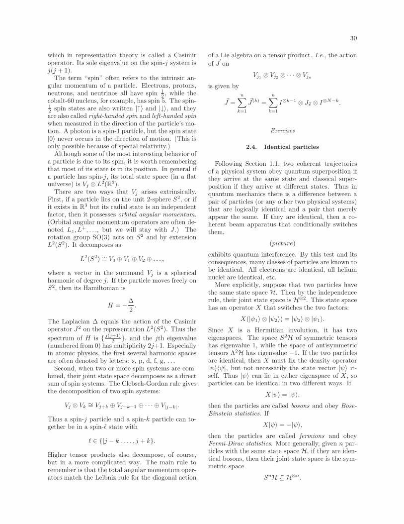
30

which in representation theory is called a Casimiroperator. Its sole eigenvalue on the spin-j system isj(j + 1).

The term “spin” often refers to the intrinsic an-gular momentum of a particle. Electrons, protons,neutrons, and neutrinos all have spin 1

2 , while thecobalt-60 nucleus, for example, has spin 5. The spin-12 spin states are also written |↑〉 and |↓〉, and theyare also called right-handed spin and left-handed spinwhen measured in the direction of the particle’s mo-tion. A photon is a spin-1 particle, but the spin state|0〉 never occurs in the direction of motion. (This isonly possible because of special relativity.)

Although some of the most interesting behavior ofa particle is due to its spin, it is worth rememberingthat most of its state is in its position. In general ifa particle has spin-j, its total state space (in a flatuniverse) is Vj ⊗ L2(R3).

There are two ways that Vj arises extrinsically.First, if a particle lies on the unit 2-sphere S2, or ifit exists in R3 but its radial state is an independentfactor, then it possesses orbital angular momentum.(Orbital angular momentum operators are often de-noted Lz, L

+, . . ., but we will stay with J .) Therotation group SO(3) acts on S2 and by extensionL2(S2). It decomposes as

L2(S2) ∼= V0 ⊕ V1 ⊕ V2 ⊕ . . . ,

where a vector in the summand Vj is a sphericalharmonic of degree j. If the particle moves freely onS2, then its Hamiltonian is

H = −∆

2.

The Laplacian ∆ equals the action of the Casimiroperator J2 on the representation L2(S2). Thus the

spectrum of H is { j(j+1)2 }, and the jth eigenvalue

(numbered from 0) has multiplicity 2j+1. Especiallyin atomic physics, the first several harmonic spacesare often denoted by letters: s, p, d, f, g, . . .

Second, when two or more spin systems are com-bined, their joint state space decomposes as a directsum of spin systems. The Clebsch-Gordan rule givesthe decomposition of two spin systems:

Vj ⊗ Vk∼= Vj+k ⊕ Vj+k−1 ⊕ · · · ⊕ V|j−k|.

Thus a spin-j particle and a spin-k particle can to-gether be in a spin-ℓ state with

ℓ ∈ {|j − k|, . . . , j + k}.

Higher tensor products also decompose, of course,but in a more complicated way. The main rule toremember is that the total angular momentum oper-ators match the Leibniz rule for the diagonal action

of a Lie algebra on a tensor product. I.e., the action

of ~J on

Vj1 ⊗ Vj2 ⊗ · · · ⊗ Vjn

is given by

~J =

n∑

k=1

~J (k) =

n∑

k=1

I⊗k−1 ⊗ J~v ⊗ I⊗N−k.

Exercises

2.4. Identical particles

Following Section 1.1, two coherent trajectoriesof a physical system obey quantum superposition ifthey arrive at the same state and classical super-position if they arrive at different states. Thus inquantum mechanics there is a difference between apair of particles (or any other two physical systems)that are logically identical and a pair that merelyappear the same. If they are identical, then a co-herent beam apparatus that conditionally switchesthem,

(picture)

exhibits quantum interference. By this test and itsconsequences, many classes of particles are known tobe identical. All electrons are identical, all heliumnuclei are identical, etc.

More explicitly, suppose that two particles havethe same state space H. Then by the independencerule, their joint state space is H⊗2. This state spacehas an operator X that switches the two factors:

X(|ψ1〉 ⊗ |ψ2〉) = |ψ2〉 ⊗ |ψ1〉.Since X is a Hermitian involution, it has twoeigenspaces. The space S2H of symmetric tensorshas eigenvalue 1, while the space of antisymmetrictensors Λ2H has eigenvalue −1. If the two particlesare identical, then X must fix the density operator|ψ〉〈ψ|, but not necessarily the state vector |ψ〉 it-self. Thus |ψ〉 can lie in either eigenspace of X , soparticles can be identical in two different ways. If

X |ψ〉 = |ψ〉,then the particles are called bosons and obey Bose-Einstein statistics. If

X |ψ〉 = −|ψ〉,then the particles are called fermions and obeyFermi-Dirac statistics. More generally, given n par-ticles with the same state space H, if they are iden-tical bosons, then their joint state space is the sym-metric space

SnH ⊆ H⊗n.

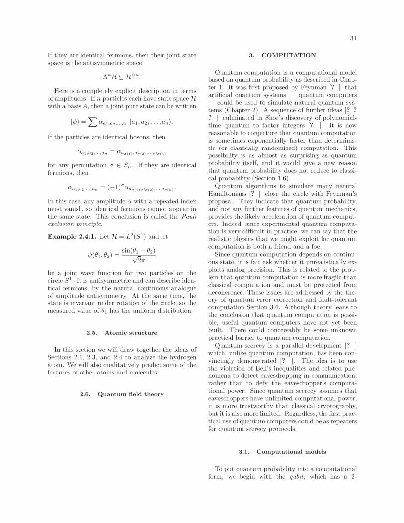
31

If they are identical fermions, then their joint statespace is the antisymmetric space

ΛnH ⊆ H⊗n.

Here is a completely explicit description in termsof amplitudes. If n particles each have state space Hwith a basis A, then a joint pure state can be written

|ψ〉 =∑

αa1,a2,...,an|a1, a2, . . . , an〉.

If the particles are identical bosons, then

αa1,a2,...,an= αaσ(1),aσ(2),...,aσ(n)

for any permutation σ ∈ Sn. If they are identicalfermions, then

αa1,a2,...,an= (−1)σαaσ(1),aσ(2),...,aσ(n)

.

In this case, any amplitude α with a repeated indexmust vanish, so identical fermions cannot appear inthe same state. This conclusion is called the Pauliexclusion principle.

Example 2.4.1. Let H = L2(S1) and let

ψ(θ1, θ2) =sin(θ1 − θ2)√

2π

be a joint wave function for two particles on thecircle S1. It is antisymmetric and can describe iden-tical fermions, by the natural continuous analogueof amplitude antisymmetry. At the same time, thestate is invariant under rotation of the circle, so themeasured value of θ1 has the uniform distribution.

2.5. Atomic structure

In this section we will draw together the ideas ofSections 2.1, 2.3, and 2.4 to analyze the hydrogenatom. We will also qualitatively predict some of thefeatures of other atoms and molecules.

2.6. Quantum field theory

3. COMPUTATION

Quantum computation is a computational modelbased on quantum probability as described in Chap-ter 1. It was first proposed by Feynman [? ] thatartificial quantum systems — quantum computers— could be used to simulate natural quantum sys-tems (Chapter 2). A sequence of further ideas [? ?? ] culminated in Shor’s discovery of polynomial-time quantum to factor integers [? ]. It is nowreasonable to conjecture that quantum computationis sometimes exponentially faster than determinis-tic (or classically randomized) computation. Thispossibility is as almost as surprising as quantumprobability itself, and it would give a new reasonthat quantum probability does not reduce to classi-cal probability (Section 1.6).

Quantum algorithms to simulate many naturalHamiltonians [? ] close the circle with Feynman’sproposal. They indicate that quantum probability,and not any further features of quantum mechanics,provides the likely acceleration of quantum comput-ers. Indeed, since experimental quantum computa-tion is very difficult in practice, we can say that therealistic physics that we might exploit for quantumcomputation is both a friend and a foe.

Since quantum computation depends on continu-ous state, it is fair ask whether it unrealistically ex-ploits analog precision. This is related to the prob-lem that quantum computation is more fragile thanclassical computation and must be protected fromdecoherence. These issues are addressed by the the-ory of quantum error correction and fault-tolerantcomputation Section 3.6. Although theory leans tothe conclusion that quantum computation is possi-ble, useful quantum computers have not yet beenbuilt. There could conceivably be some unknownpractical barrier to quantum computation.

Quantum secrecy is a parallel development [? ]which, unlike quantum computation, has been con-vincingly demonstrated [? ]. The idea is to usethe violation of Bell’s inequalities and related phe-nomena to detect eavesdropping in communication,rather than to defy the eavesdropper’s computa-tional power. Since quantum secrecy assumes thateavesdroppers have unlimited computational power,it is more trustworthy than classical cryptography,but it is also more limited. Regardless, the first prac-tical use of quantum computers could be as repeatersfor quantum secrecy protocols.

3.1. Computational models

To put quantum probability into a computationalform, we begin with the qubit, which has a 2-

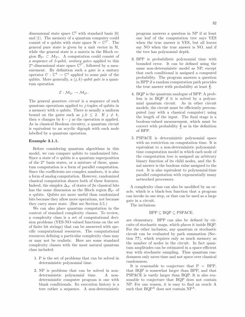
32

dimensional state space C2 with standard basis |0〉and |1〉. The memory of a quantum computer couldconsist of n qubits with state space H = C2n

. Thegeneral pure state is given by a unit vector in H,while the general state is a matrix in the Bloch re-gion B2n ⊂ M2n . A computation could consist ofa sequence of 2-qubit, unitary gates applied to this2n-dimensional state space C2n

, followed by a mea-surement. By definition such a gate is a unitaryoperator U : C4 → C4 applied to some pair of thequbits. More generally, a (j, k)-qubit gate is a quan-tum operation

E :M2j →M2k .

The general quantum circuit is a sequence of suchquantum operations applied to j-tuples of qubits ina memory with n qubits. There is usually a uniformbound on the gates such as j, k ≤ 2. If j 6= k,then n changes by k− j as the operation is applied.As in classical Boolean circuitry, a quantum circuitis equivalent to an acyclic digraph with each nodelabelled by a quantum operation.

Example 3.1.1.

Before considering quantum algorithms in thismodel, we can compare qubits to randomized bits.Since a state of n qubits is a quantum superpositionof the 2n basis states, or a mixture of these, quan-tum computation is a form of parallel computation.Since the coefficients are complex numbers, it is alsoa form of analog computation. However, randomizedclassical computation shares both of these features.Indeed, the simplex ∆4n of states of 2n classical bitshas the same dimension as the Bloch region B2n ofn qubits. Qubits are more useful than randomizedbits because they allow more operations, not becausethey carry more state. (But see Section 3.5.)

We can also place quantum computation in thecontext of standard complexity classes. To review,a complexity class is a set of computational deci-sion problems (YES-NO-valued functions on the setof finite bit strings) that can be answered with spe-cific computational resources. The computationalresources defining a particular complexity class mayor may not be realistic. Here are some standardcomplexity classes with the most natural quantumclass included:

1. P is the set of problems that can be solved indeterministic polynomial time.

2. NP is problems that can be solved in non-deterministic polynomial time. A non-deterministic computer program is one withblank conditionals. Its execution history is atree rather a sequence. A non-deterministic

program answers a question in NP if at leastone leaf of the computation tree says YESwhen the true answer is YES, but all leavessay NO when the true answer is NO, and ifthe tree has polynomial depth.

3. BPP is probabilistic polynomial time withbounded error. It can be defined using thesame non-deterministic model as NP, exceptthat each conditional is assigned a computedprobability. The program answers a questionin BPP if a random computation path providesthe true answer with probability at least 2

3 .

4. BQP is the quantum analogue of BPP. A prob-lem is in BQP if it is solved by a polyno-mial quantum circuit. As in other circuitmodels, the circuit must be efficiently precom-puted (say with a classical computer) usingthe length of the input. The final stage is aboolean-valued measurement, which must becorrect with probability 2

3 as in the definitionof BPP.

5. PSPACE is deterministic polynomial spacewith no restriction on computation time. It isequivalent to a non-deterministic polynomial-time computation model in which each node ofthe computation tree is assigned an arbitrarybinary function of its child nodes, and the fi-nal answer is the boolean value assigned to theroot. It is also equivalent to polynomial-timeparallel computation with exponentially manynetworked processors.

A complexity class can also be modified by an or-acle, which is a black-box function that a programcan invoke in one step, or that can be used as a largegate in a circuit.

The inclusions

BPP ⊆ BQP ⊆ PSPACE.

are elementary. BPP can also be defined by cir-cuits of stochastic maps, which places it inside BQP.For the other inclusion, any quantum or stochasticcircuit can be evaluated by path summation (Sec-tion ??), which requires only as much memory asthe number of nodes in the circuit. In fact quan-tum amplitudes can be estimated in a space-efficientway with stochastic sampling. Thus quantum ran-domness only saves time and not space over classicalrandomness.

It is reasonable to conjecture that P = BPP,that BQP is somewhat larger than BPP, and thatPSPACE is vastly larger than BQP. It is also rea-sonable to conjecture that BQP does not containNP. For one reason, it is easy to find an oracle Asuch that BQPA does not contain NPA.

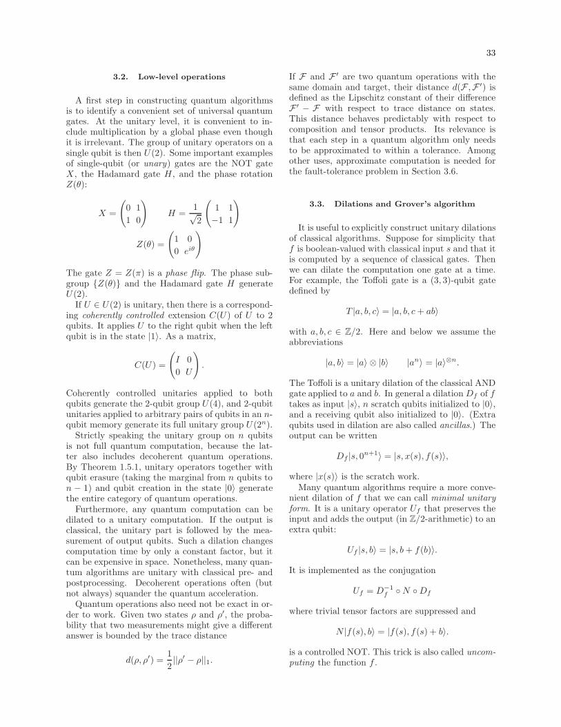
33

3.2. Low-level operations

A first step in constructing quantum algorithmsis to identify a convenient set of universal quantumgates. At the unitary level, it is convenient to in-clude multiplication by a global phase even thoughit is irrelevant. The group of unitary operators on asingle qubit is then U(2). Some important examplesof single-qubit (or unary) gates are the NOT gateX , the Hadamard gate H , and the phase rotationZ(θ):

X =

(0 1

1 0

)H =

1√2

(1 1

−1 1

)

Z(θ) =

(1 0

0 eiθ

)

The gate Z = Z(π) is a phase flip. The phase sub-group {Z(θ)} and the Hadamard gate H generateU(2).

If U ∈ U(2) is unitary, then there is a correspond-ing coherently controlled extension C(U) of U to 2qubits. It applies U to the right qubit when the leftqubit is in the state |1〉. As a matrix,

C(U) =

(I 0

0 U

).

Coherently controlled unitaries applied to bothqubits generate the 2-qubit group U(4), and 2-qubitunitaries applied to arbitrary pairs of qubits in an n-qubit memory generate its full unitary group U(2n).

Strictly speaking the unitary group on n qubitsis not full quantum computation, because the lat-ter also includes decoherent quantum operations.By Theorem 1.5.1, unitary operators together withqubit erasure (taking the marginal from n qubits ton − 1) and qubit creation in the state |0〉 generatethe entire category of quantum operations.

Furthermore, any quantum computation can bedilated to a unitary computation. If the output isclassical, the unitary part is followed by the mea-surement of output qubits. Such a dilation changescomputation time by only a constant factor, but itcan be expensive in space. Nonetheless, many quan-tum algorithms are unitary with classical pre- andpostprocessing. Decoherent operations often (butnot always) squander the quantum acceleration.

Quantum operations also need not be exact in or-der to work. Given two states ρ and ρ′, the proba-bility that two measurements might give a differentanswer is bounded by the trace distance

d(ρ, ρ′) =1

2||ρ′ − ρ||1.

If F and F ′ are two quantum operations with thesame domain and target, their distance d(F ,F ′) isdefined as the Lipschitz constant of their differenceF ′ − F with respect to trace distance on states.This distance behaves predictably with respect tocomposition and tensor products. Its relevance isthat each step in a quantum algorithm only needsto be approximated to within a tolerance. Amongother uses, approximate computation is needed forthe fault-tolerance problem in Section 3.6.

3.3. Dilations and Grover’s algorithm

It is useful to explicitly construct unitary dilationsof classical algorithms. Suppose for simplicity thatf is boolean-valued with classical input s and that itis computed by a sequence of classical gates. Thenwe can dilate the computation one gate at a time.For example, the Toffoli gate is a (3, 3)-qubit gatedefined by

T |a, b, c〉 = |a, b, c+ ab〉

with a, b, c ∈ Z/2. Here and below we assume theabbreviations

|a, b〉 = |a〉 ⊗ |b〉 |an〉 = |a〉⊗n.

The Toffoli is a unitary dilation of the classical ANDgate applied to a and b. In general a dilation Df of ftakes as input |s〉, n scratch qubits initialized to |0〉,and a receiving qubit also initialized to |0〉. (Extraqubits used in dilation are also called ancillas.) Theoutput can be written

Df |s, 0n+1〉 = |s, x(s), f(s)〉,

where |x(s)〉 is the scratch work.Many quantum algorithms require a more conve-

nient dilation of f that we can call minimal unitaryform. It is a unitary operator Uf that preserves theinput and adds the output (in Z/2-arithmetic) to anextra qubit:

Uf |s, b〉 = |s, b+ f(b)〉.

It is implemented as the conjugation

Uf = D−1f ◦N ◦Df

where trivial tensor factors are suppressed and

N |f(s), b〉 = |f(s), f(s) + b〉.

is a controlled NOT. This trick is also called uncom-puting the function f .

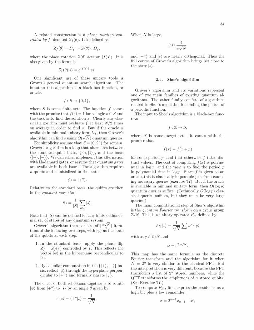
34

A related construction is a phase rotation con-trolled by f , denoted Zf(θ). It is defined as

Zf (θ) = D−1f ◦ Z(θ) ◦Df ,

where the phase rotation Z(θ) acts on |f(s)〉. It isalso given by the formula

Zf (θ)|s〉 = eif(s)θ|s〉.

One significant use of these unitary tools isGrover’s general quantum search algorithm. Theinput to this algorithm is a black-box function, ororacle,

f : S → {0, 1},

where S is some finite set. The function f comeswith the promise that f(s) = 1 for a single s ∈ S andthe task is to find the solution s. Clearly any clas-sical algorithm must evaluate f at least N/2 timeson average in order to find s. But if the oracle isavailable in minimal unitary form Uf , then Grover’s

algorithm can find s using O(√N) quantum queries.

For simplicity assume that S = [0, 2n) for some n.Grover’s algorithm is a loop that alternates betweenthe standard qubit basis, {|0〉, |1〉}, and the basis{|+〉, |−〉}. We can either implement this alternationwith Hadamard gates, or assume that quantum gatesare available in both bases. The algorithm requiresn qubits and is initialized in the state

|ψ〉 = |+n〉.

Relative to the standard basis, the qubits are thenin the constant pure state

|S〉 =1

|S|∑

s∈S

|s〉.

Note that |S〉 can be defined for any finite orthonor-mal set of states of any quantum system.

Grover’s algorithm then consists of ⌊π√

N4 ⌋ itera-

tions of the following two steps, with |ψ〉 as the stateof the qubits at each step.

1. In the standard basis, apply the phase flipZf = Zf (π) controlled by f . This reflects thevector |ψ〉 in the hyperplane perpendicular to|s〉.

2. By a similar computation in the {|+〉, |−〉} ba-sis, reflect |φ〉 through the hyperplane perpen-dicular to |+n〉 and formally negate |ψ〉.

The effect of both reflections together is to rotate|ψ〉 from |+n〉 to |s〉 by an angle θ given by

sin θ = 〈+n|s〉 =1√N.

When N is large,

θ ≈ 4

π√N

and |+n〉 and |s〉 are nearly orthogonal. Thus thefull course of Grover’s algorithm brings |ψ〉 close tothe state |s〉.

3.4. Shor’s algorithm

Grover’s algorithm and its variations representone of two main families of existing quantum al-gorithms. The other family consists of algorithmsrelated to Shor’s algorithm for finding the period ofa periodic function.

The input to Shor’s algorithm is a black-box func-tion

f : Z→ S,

where S is some target set. It comes with thepromise that

f(x) = f(x+ p)

for some period p, and that otherwise f takes dis-tinct values. The cost of computing f(x) is polyno-mial in log x, and the task is to find the period pin polynomial time in log p. Since f is given as anoracle, this is classically impossible just from count-ing necessary queries (exercise ??). But if the oracleis available in minimal unitary form, then O(log p)quantum queries suffice. (Technically O(log p) clas-sical queries suffices, but they must be very largequeries.)

The main computational step of Shor’s algorithmis the quantum Fourier transform on a cyclic groupZ/N . This is a unitary operator FN defined by

FN |x〉 =1√N

∑ωxy|y〉

with x, y ∈ Z/N and

ω = e2πi/N .

This map has the same formula as the discreteFourier transform and the algorithm for it whenN = 2n is very similar to the classical FFT. Butthe interpretation is very different, because the FFTtransforms a list of 2n stored numbers, while theQFT transforms the amplitudes of n stored qubits.(See Exercise ??.)

To compute F2n , first express the residue x as ahigh bit plus a low remainder,

x = 2n−1xn−1 + x′,

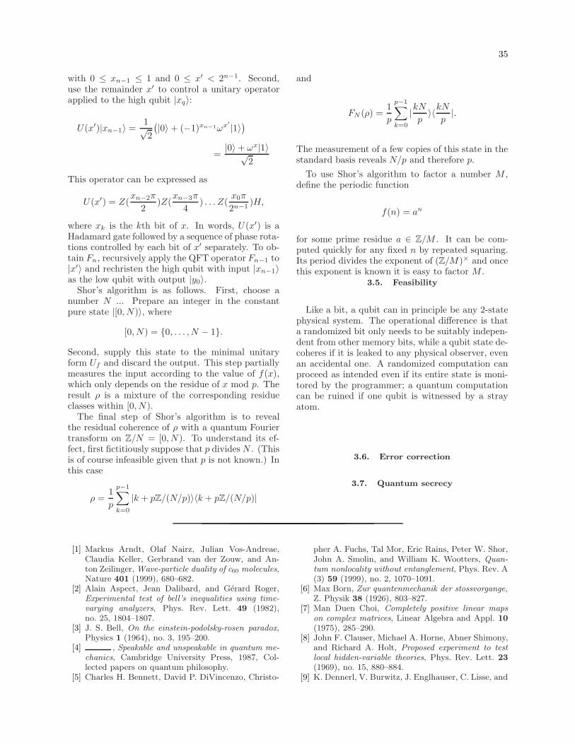
35

with 0 ≤ xn−1 ≤ 1 and 0 ≤ x′ < 2n−1. Second,use the remainder x′ to control a unitary operatorapplied to the high qubit |xq〉:

U(x′)|xn−1〉 =1√2

(|0〉+ (−1)xn−1ωx′ |1〉

)

=|0〉+ ωx|1〉√

2

This operator can be expressed as

U(x′) = Z(xn−2π

2)Z(

xn−3π

4) . . . Z(

x0π

2n−1)H,

where xk is the kth bit of x. In words, U(x′) is aHadamard gate followed by a sequence of phase rota-tions controlled by each bit of x′ separately. To ob-tain Fn, recursively apply the QFT operator Fn−1 to|x′〉 and rechristen the high qubit with input |xn−1〉as the low qubit with output |y0〉.

Shor’s algorithm is as follows. First, choose anumber N ... Prepare an integer in the constantpure state |[0, N)〉, where

[0, N) = {0, . . . , N − 1}.

Second, supply this state to the minimal unitaryform Uf and discard the output. This step partiallymeasures the input according to the value of f(x),which only depends on the residue of x mod p. Theresult ρ is a mixture of the corresponding residueclasses within [0, N).

The final step of Shor’s algorithm is to revealthe residual coherence of ρ with a quantum Fouriertransform on Z/N = [0, N). To understand its ef-fect, first fictitiously suppose that p dividesN . (Thisis of course infeasible given that p is not known.) Inthis case

ρ =1

p

p−1∑

k=0

|k + pZ/(N/p)〉〈k + pZ/(N/p)|

and

FN (ρ) =1

p

p−1∑

k=0

|kNp〉〈kN

p|.

The measurement of a few copies of this state in thestandard basis reveals N/p and therefore p.

To use Shor’s algorithm to factor a number M ,define the periodic function

f(n) = an

for some prime residue a ∈ Z/M . It can be com-puted quickly for any fixed n by repeated squaring.Its period divides the exponent of (Z/M)× and oncethis exponent is known it is easy to factor M .

3.5. Feasibility

Like a bit, a qubit can in principle be any 2-statephysical system. The operational difference is thata randomized bit only needs to be suitably indepen-dent from other memory bits, while a qubit state de-coheres if it is leaked to any physical observer, evenan accidental one. A randomized computation canproceed as intended even if its entire state is moni-tored by the programmer; a quantum computationcan be ruined if one qubit is witnessed by a strayatom.

3.6. Error correction

3.7. Quantum secrecy

[1] Markus Arndt, Olaf Nairz, Julian Vos-Andreae,Claudia Keller, Gerbrand van der Zouw, and An-ton Zeilinger, Wave-particle duality of c60 molecules,Nature 401 (1999), 680–682.

[2] Alain Aspect, Jean Dalibard, and Gerard Roger,Experimental test of bell’s inequalities using time-

varying analyzers, Phys. Rev. Lett. 49 (1982),no. 25, 1804–1807.

[3] J. S. Bell, On the einstein-podolsky-rosen paradox,Physics 1 (1964), no. 3, 195–200.

[4] , Speakable and unspeakable in quantum me-

chanics, Cambridge University Press, 1987, Col-lected papers on quantum philosophy.

[5] Charles H. Bennett, David P. DiVincenzo, Christo-

pher A. Fuchs, Tal Mor, Eric Rains, Peter W. Shor,John A. Smolin, and William K. Wootters, Quan-

tum nonlocality without entanglement, Phys. Rev. A(3) 59 (1999), no. 2, 1070–1091.

[6] Max Born, Zur quantenmechanik der stossvorgange,Z. Physik 38 (1926), 803–827.

[7] Man Duen Choi, Completely positive linear maps

on complex matrices, Linear Algebra and Appl. 10

(1975), 285–290.[8] John F. Clauser, Michael A. Horne, Abner Shimony,

and Richard A. Holt, Proposed experiment to test

local hidden-variable theories, Phys. Rev. Lett. 23

(1969), no. 15, 880–884.[9] K. Dennerl, V. Burwitz, J. Englhauser, C. Lisse, and

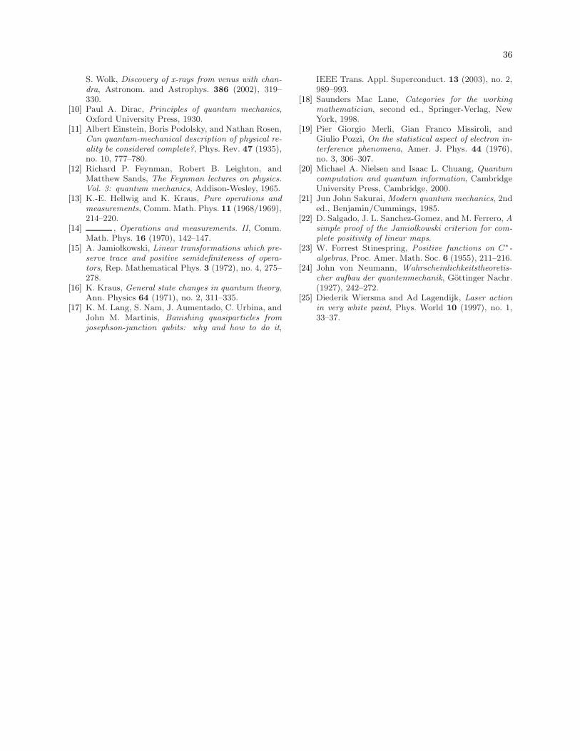
36

S. Wolk, Discovery of x-rays from venus with chan-

dra, Astronom. and Astrophys. 386 (2002), 319–330.

[10] Paul A. Dirac, Principles of quantum mechanics,Oxford University Press, 1930.

[11] Albert Einstein, Boris Podolsky, and Nathan Rosen,Can quantum-mechanical description of physical re-

ality be considered complete?, Phys. Rev. 47 (1935),no. 10, 777–780.

[12] Richard P. Feynman, Robert B. Leighton, andMatthew Sands, The Feynman lectures on physics.

Vol. 3: quantum mechanics, Addison-Wesley, 1965.[13] K.-E. Hellwig and K. Kraus, Pure operations and

measurements, Comm. Math. Phys. 11 (1968/1969),214–220.

[14] , Operations and measurements. II, Comm.Math. Phys. 16 (1970), 142–147.

[15] A. Jamio lkowski, Linear transformations which pre-

serve trace and positive semidefiniteness of opera-

tors, Rep. Mathematical Phys. 3 (1972), no. 4, 275–278.

[16] K. Kraus, General state changes in quantum theory,Ann. Physics 64 (1971), no. 2, 311–335.

[17] K. M. Lang, S. Nam, J. Aumentado, C. Urbina, andJohn M. Martinis, Banishing quasiparticles from

josephson-junction qubits: why and how to do it,

IEEE Trans. Appl. Superconduct. 13 (2003), no. 2,989–993.

[18] Saunders Mac Lane, Categories for the working

mathematician, second ed., Springer-Verlag, NewYork, 1998.

[19] Pier Giorgio Merli, Gian Franco Missiroli, andGiulio Pozzi, On the statistical aspect of electron in-

terference phenomena, Amer. J. Phys. 44 (1976),no. 3, 306–307.

[20] Michael A. Nielsen and Isaac L. Chuang, Quantum

computation and quantum information, CambridgeUniversity Press, Cambridge, 2000.

[21] Jun John Sakurai, Modern quantum mechanics, 2nded., Benjamin/Cummings, 1985.

[22] D. Salgado, J. L. Sanchez-Gomez, and M. Ferrero, A

simple proof of the Jamiolkowski criterion for com-

plete positivity of linear maps.[23] W. Forrest Stinespring, Positive functions on C∗-

algebras, Proc. Amer. Math. Soc. 6 (1955), 211–216.[24] John von Neumann, Wahrscheinlichkeitstheoretis-

cher aufbau der quantenmechanik, Gottinger Nachr.(1927), 242–272.

[25] Diederik Wiersma and Ad Lagendijk, Laser action

in very white paint, Phys. World 10 (1997), no. 1,33–37.