A Constraint Solver for Software Engineering:

Finding Models and Cores of Large Relational

Specifications

by

Emina Torlak

M.Eng., Massachusetts Institute of Technology (2004)

B.Sc., Massachusetts Institute of Technology (2003)

Submitted to the Department of Electrical Engineering and ComputerScience

in partial fulfillment of the requirements for the degree of

Doctor of Philosophy

at the

MASSACHUSETTS INSTITUTE OF TECHNOLOGY

February 2009

c© Massachusetts Institute of Technology 2009. All rights reserved.

Author . . . . . . . . . . . . . . . . . . . . . . . . . . . . . . . . . . . . . . . . . . . . . . . . . . . . . . . . . . . . . .Department of Electrical Engineering and Computer Science

December 8, 2008

Certified by. . . . . . . . . . . . . . . . . . . . . . . . . . . . . . . . . . . . . . . . . . . . . . . . . . . . . . . . . .Daniel Jackson

ProfessorThesis Supervisor

Accepted by . . . . . . . . . . . . . . . . . . . . . . . . . . . . . . . . . . . . . . . . . . . . . . . . . . . . . . . . .Professor Terry P. Orlando

Chairman, Department Committee on Graduate Students

A Constraint Solver for Software Engineering: FindingModels and Cores of Large Relational Specifications

byEmina Torlak

Submitted to the Department of Electrical Engineering and Computer Scienceon December 8, 2008, in partial fulfillment of the

requirements for the degree ofDoctor of Philosophy

Abstract

Relational logic is an attractive candidate for a software description language, be-cause both the design and implementation of software often involve reasoning aboutrelational structures: organizational hierarchies in the problem domain, architecturalconfigurations in the high level design, or graphs and linked lists in low level code. Un-til recently, however, frameworks for solving relational constraints have had limitedapplicability. Designed to analyze small, hand-crafted models of software systems,current frameworks perform poorly on specifications that are large or that have par-tially known solutions.

This thesis presents an efficient constraint solver for relational logic, with recentapplications to design analysis, code checking, test-case generation, and declarativeconfiguration. The solver provides analyses for both satisfiable and unsatisfiablespecifications—a finite model finder for the former and a minimal unsatisfiable coreextractor for the latter. It works by translating a relational problem to a booleansatisfiability problem; applying an off-the-shelf SAT solver to the resulting formula;and converting the SAT solver’s output back to the relational domain.

The idea of solving relational problems by reduction to SAT is not new. The corecontributions of this work, instead, are new techniques for expanding the capacityand applicability of SAT-based engines. They include: a new interface to SAT thatextends relational logic with a mechanism for specifying partial solutions; a newtranslation algorithm based on sparse matrices and auto-compacting circuits; a newsymmetry detection technique that works in the presence of partial solutions; and anew core extraction algorithm that recycles inferences made at the boolean level tospeed up core minimization at the specification level.

Thesis Supervisor: Daniel JacksonTitle: Professor

Acknowledgments

Working on this thesis has been a challenging, rewarding and, above all, wonderfulexperience. I am deeply grateful to the people who have shared it with me:

To my advisor, Daniel Jackson, for his guidance, support, enthusiasm, and agreat sense of humor. He has helped me become not only a better researcher,but a better writer and a better advocate for my ideas.

To my thesis readers, David Karger and Sharad Malik, for their insights andexcellent comments.

To my friends and colleagues in the Software Design Group—Felix Chang, GregDennis, Jonathan Edwards, Eunsuk Kang, Sarfraz Khurshid, Carlos Pacheco,Derek Rayside, Robert Seater, Ilya Shlyakhter, Mana Taghdiri and MandanaVaziri—for their companionship and for many lively discussions of researchideas, big and small. Ilya’s work on Alloy3 paved the way for this disserta-tion; Greg, Mana and Felix’s early adoption of the solver described here wasinstrumental to its design and development.

To my husband Aled for his love, patience and encouragement; to my sisterAlma for her boundless warmth and kindness; and to my mother Edina for herunrelenting support and for giving me life more than once.

I dedicate this thesis to my mother and to the memory of my father.

The first challenge for computing science is to discover how to maintain order in a finite,but very large, discrete universe that is intricately intertwined.

E. W. Dijkstra, 1979

Contents

1 Introduction 131.1 Bounded relational logic . . . . . . . . . . . . . . . . . . . . . . . . . 151.2 Finite model finding . . . . . . . . . . . . . . . . . . . . . . . . . . . 171.3 Minimal unsatisfiable core extraction . . . . . . . . . . . . . . . . . . 231.4 Summary of contributions . . . . . . . . . . . . . . . . . . . . . . . . 27

2 From Relational to Boolean Logic 312.1 Bounded relational logic . . . . . . . . . . . . . . . . . . . . . . . . . 322.2 Translating bounded relational logic to SAT . . . . . . . . . . . . . . 35

2.2.1 Translation algorithm . . . . . . . . . . . . . . . . . . . . . . . 352.2.2 Sparse-matrix representation of relations . . . . . . . . . . . . 372.2.3 Sharing detection at the boolean level . . . . . . . . . . . . . . 40

2.3 Related work . . . . . . . . . . . . . . . . . . . . . . . . . . . . . . . 442.3.1 Type-based representation of relations . . . . . . . . . . . . . 442.3.2 Sharing detection at the problem level . . . . . . . . . . . . . 462.3.3 Multidimensional sparse matrices . . . . . . . . . . . . . . . . 472.3.4 Auto-compacting circuits . . . . . . . . . . . . . . . . . . . . . 50

2.4 Experimental results . . . . . . . . . . . . . . . . . . . . . . . . . . . 51

3 Detecting Symmetries 553.1 Symmetries in model extension . . . . . . . . . . . . . . . . . . . . . 563.2 Complete and greedy symmetry detection . . . . . . . . . . . . . . . 60

3.2.1 Symmetries via graph automorphism detection . . . . . . . . . 613.2.2 Symmetries via greedy base partitioning . . . . . . . . . . . . 63

3.3 Experimental results . . . . . . . . . . . . . . . . . . . . . . . . . . . 683.4 Related work . . . . . . . . . . . . . . . . . . . . . . . . . . . . . . . 70

3.4.1 Symmetries in traditional model finding . . . . . . . . . . . . 713.4.2 Symmetries in constraint programming . . . . . . . . . . . . . 72

4 Finding Minimal Cores 754.1 A small example . . . . . . . . . . . . . . . . . . . . . . . . . . . . . 76

4.1.1 A toy list specification . . . . . . . . . . . . . . . . . . . . . . 764.1.2 Sample analyses . . . . . . . . . . . . . . . . . . . . . . . . . . 77

4.2 Core extraction with a resolution engine . . . . . . . . . . . . . . . . 814.2.1 Resolution-based analysis . . . . . . . . . . . . . . . . . . . . 82

7

4.2.2 Recycling core extraction . . . . . . . . . . . . . . . . . . . . . 864.2.3 Correctness and minimality of RCE . . . . . . . . . . . . . . . 88

4.3 Experimental results . . . . . . . . . . . . . . . . . . . . . . . . . . . 894.4 Related work . . . . . . . . . . . . . . . . . . . . . . . . . . . . . . . 93

4.4.1 Minimal core extraction . . . . . . . . . . . . . . . . . . . . . 934.4.2 Clause recycling . . . . . . . . . . . . . . . . . . . . . . . . . . 94

5 Conclusion 975.1 Discussion . . . . . . . . . . . . . . . . . . . . . . . . . . . . . . . . . 985.2 Future work . . . . . . . . . . . . . . . . . . . . . . . . . . . . . . . . 101

5.2.1 Bitvector arithmetic and inductive definitions . . . . . . . . . 1015.2.2 Special-purpose translation for logic fragments . . . . . . . . . 1025.2.3 Heuristics for variable and constraint ordering . . . . . . . . . 103

8

List of Figures

1-1 A hard Sudoku puzzle . . . . . . . . . . . . . . . . . . . . . . . . . . . 131-2 Sudoku in bounded relational logic, Alloy, FOL, and FOL/ID . . . . . . . 181-3 Solution for the sample Sudoku puzzle . . . . . . . . . . . . . . . . . . . 191-4 Effect of partial models on the performance of SAT-based model finders . 211-5 Effect of partial models on the performance of a dedicated Sudoku solver . 221-6 An unsatisfiable Sudoku puzzle and its core . . . . . . . . . . . . . . . . 241-7 Comparison of SAT-based core extractors on 100 unsatisfiable Sudokus . . 261-8 Summary of contributions . . . . . . . . . . . . . . . . . . . . . . . . . 28

2-1 Syntax and semantics of bounded relational logic . . . . . . . . . . . . . 332-2 A toy filesystem . . . . . . . . . . . . . . . . . . . . . . . . . . . . . . 342-3 Translation rules for bounded relational logic . . . . . . . . . . . . . . . 362-4 A sample translation . . . . . . . . . . . . . . . . . . . . . . . . . . . . 382-5 Sparse representation of translation matrices . . . . . . . . . . . . . . . . 392-6 Computing the d-reachable descendants of a CBC node . . . . . . . . . . 412-7 A non-compact boolean circuit and its compact equivalents . . . . . . . . 432-8 GCRS and ECRS representations for multidimensional sparse matrices . . 482-9 An example of a non-optimal two-level rewrite rule . . . . . . . . . . . . 52

3-1 Isomorphisms of the filesystem model . . . . . . . . . . . . . . . . . . . 573-2 Isomorphisms of an invalid binding for the toy filesystem . . . . . . . . . 573-3 Complete symmetry detection via graph automorphism . . . . . . . . . . 623-4 A toy filesystem with no partial model . . . . . . . . . . . . . . . . . . . 643-5 Symmetry detection via greedy base partitioning . . . . . . . . . . . . . 663-6 Microstructure of a CSP . . . . . . . . . . . . . . . . . . . . . . . . . . 74

4-1 A toy list specification . . . . . . . . . . . . . . . . . . . . . . . . . . . 784-2 The resolution rule for propositional logic . . . . . . . . . . . . . . . . . 844-3 Resolution-based analysis of (a = b) ∧ (b = c) ∧ ¬(a⇒ c) . . . . . . . . . 844-4 Core extraction algorithms . . . . . . . . . . . . . . . . . . . . . . . . . 87

9

10

List of Tables

1.1 Recent applications of Kodkod . . . . . . . . . . . . . . . . . . . . . . . 29

2.1 Simplification rules for CBCs . . . . . . . . . . . . . . . . . . . . . . . . 422.2 Evaluation of Kodkod’s translation optimizations . . . . . . . . . . . . . 53

3.1 Evaluation of symmetry detection algorithms . . . . . . . . . . . . . . . 69

4.1 Evaluation of minimal core extractors . . . . . . . . . . . . . . . . . . . 904.2 Evaluation of minimal core extractors based on problem difficulty . . . . . 91

5.1 Features of state-of-the-art model finders . . . . . . . . . . . . . . . . . 99

11

12

Chapter 1

Introduction

Puzzles with simple rules can be surprisingly hard to solve, even when a part of thesolution is already known. Take Sudoku, for example. It is a logic game played on apartially completed 9×9 grid, like the one in Fig. 1-1. The goal is simply to fill in theblanks so that the numbers 1 through 9 appear exactly once in every row, column,and heavily boxed region of the grid. Each puzzle has a unique solution, and manyare easily solved. Yet some are ‘very hard.’ Target completion time for the puzzle inFig. 1-1, for example, is 30 minutes [58].

6 2 5

1 8 6 2

3 4

6 7 8

4 2 5

9 8

5 4 9 3

2 1 4

3 5 7

Figure 1-1: A hard Sudoku puzzle [58].

Software engineering is full of problems like Sudoku—where the rules are easyto describe, parts of the solution are known, but the task of filling in the blanks iscomputationally intractable. Examples include, most notably, declarative configura-tion problems such as network configuration [99], installation management [133], andscheduling [149]. The configuration task usually involves extending a valid config-uration with one or more new components so that certain validity constraints arepreserved. To install a new package on a Linux machine, for example, an installa-tion manager needs to find a subset of packages in the Linux distribution, includingthe desired package, which can be added to the installation so that all package de-pendencies are met. Also related are the problems of declarative analysis: softwaredesign analysis [69], bounded code verification against rich structural specifications

13

[31, 34, 126, 138], and declarative test-case generation [77, 114, 134].Automatic solutions to problems like Sudoku and declarative configuration usually

come in two flavors: a special-purpose solver or a special-purpose translator to somelogic, used either with an off-the-shelf SAT solver or, since recently, an SMT solver[38, 53, 9, 29] that can also reason about linear integer and bitvector arithmetic.An expertly implemented special-purpose solver is likely to perform better than atranslation-based alternative, simply because a custom solver can be guided withdomain-specific knowledge that may be hard (or impossible) to use effectively in atranslation. But crafting an efficient search algorithm is tricky, and with the advancesin SAT solving technology, the performance benefits of implementing a custom solvertend to be negligible [53]. Even for a problem as simple as Sudoku, with many knownspecial-purpose inference rules, SAT-based approaches [86, 144] are competitive withhand-crafted solvers (e.g. [141]).

Reducing a high-level problem description to SAT is not easy, however, since aboolean encoding has to contain just the right amount and kind of information toelicit the best performance from the SAT solver. If the encoding includes too manyredundant formulas, the solver will slow down significantly [119, 139, 41]. At thesame time, introducing certain kinds of redundancy into the encoding, in the formof symmetry breaking [27, 116] or reconvergence [150] clauses, can yield dramaticimprovements in solving times.

The challenges of using SAT for declarative configuration and analysis are notlimited to finding the most effective encoding. When a SAT solver fails to find asatisfying assignment for the translation of a problem, many applications need toknow what caused the failure and correct it. For example, if a software packagecannot be installed because it conflicts with one or more existing packages, a SAT-based installation manager such as OPIUM [133] needs to identify (and remove) theconflicting packages. It does this by analyzing the proof of unsatisfiability producedby the SAT solver to find an unsatisfiable subset of the translation clauses knownas an unsatisfiable core. Once extracted from the proof, the boolean core needs tomapped back to the conflicting constraints in the problem domain. The problemdomain core, in turn, has to be minimized before corrective action is taken becauseit may contain constraints which do not contribute to its unsatisfiability.

This thesis presents a framework that facilitates easy and efficient use of SAT fordeclarative configuration and analysis. The user of the framework provides just ahigh-level description of the problem—in a logic that underlies many software designlanguages [2, 143, 123, 69]—and a partial solution, if one is available. The frameworkthen does the rest: efficient translation to SAT, interpretation of the SAT instance interms of problem-domain concepts, and, in the case of unsatisfiability, interpretationand minimization of the unsatisfiable core. The key algorithms used for SAT encoding[131] and core minimization [129] are the main technical contributions of this work;the main methodological contribution is the idea of separating the description of theproblem from the description of its partial solution [130]. The embodiment of thesecontributions, called Kodkod, has so far been used in a variety of applications fordeclarative configuration [100, 149], design analysis [21], bounded code verification[31, 34, 126], and automated test-case generation [114, 134].

14

1.1 Bounded relational logic

Kodkod is based on the “relational logic” of Alloy [69], consisting essentially of afirst-order logic augmented with the operators of the relational calculus [127]. Theinclusion of transitive closure extends the expressiveness beyond standard first-orderlogics, and allows the encoding of common reachability constraints that otherwisecould not be expressed. In contrast to specification languages (such as Z [123], B[2], and OCL [143]) that are based on set-theoretic logics, Alloy’s relational logic wasdesigned to have a stronger connection to data modeling languages (such as ER [22]and SDM [62]), a more uniform syntax, and a simpler semantics. Alloy’s logic treatseverything as a relation: sets as relations of arity one and scalars as singleton sets.Function application is modeled as relational join, and an out-of-domain applicationresults in the empty set, dispensing with the need for special notions of undefinedness.The use of multi-arity relations (in contrast to functions over sets) is a critical factorin Alloy being first order and amenable to automatic analysis. The choice of this logicfor Kodkod was thus based not only on its simplicity but also on its analyzability.

Kodkod extends the logic of Alloy with the notion of relational bounds. A boundedrelational specification is a collection of constraints on relational variables of any aritythat are bound above and below by relational constants (i.e. sets of tuples). Allbounding constants consist of tuples that are drawn from the same finite universe ofuninterpreted elements. The upper bound specifies the tuples that a relation maycontain; the lower bound specifies the tuples that it must contain.

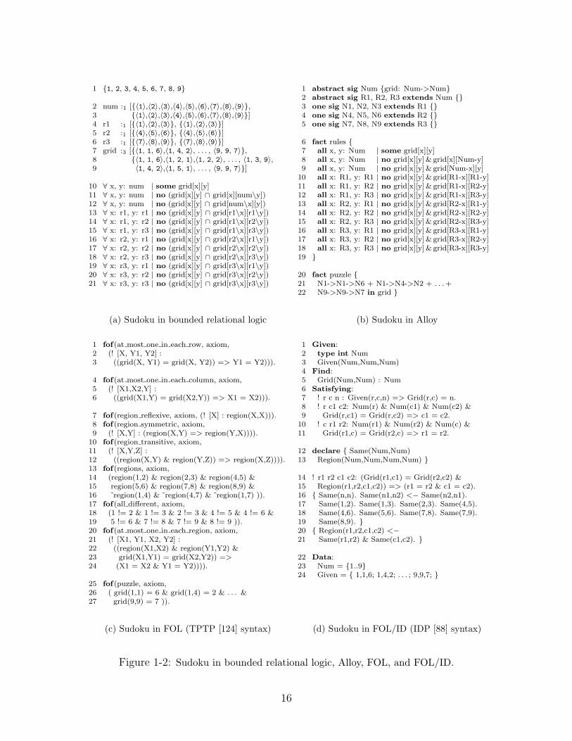
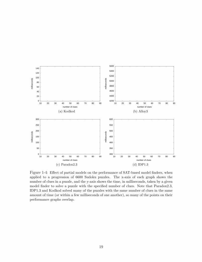
Figure 1-2a shows a snippet of bounded relational logic1 that describes the Sudokupuzzle from Fig. 1-1. It consists of three parts: the universe of discourse (line 1); thebounds on free variables that encode the assertional knowledge about the problem(lines 2-7), such as the initial state of the grid; and the constraints on the boundedvariables that encode definitional knowledge about the problem (lines 10-21), i.e. therules of the game.

The bounds specification is straightforward. The unary relation num (line 2)provides a handle on the set of numbers used in the game. As this set is constant, therelation has the same lower and upper bound. The relations r1, r2 and r3 (lines 4-6)partition the numbers into three consecutive, equally-sized intervals. The ternaryrelation grid (line 7) models the Sudoku grid as a mapping from cells, defined by theirrow and column coordinates, to numbers. The set {〈1, 1, 6〉, 〈1, 4, 2〉, . . . , 〈9, 9,7〉} specifies the lower bound on the grid relation; these are the mappings of cells tonumbers that are given in Fig. 1-1.2 The upper bound on its value is the lower boundaugmented with the bindings from the coordinates of the empty cells, such as the cellin the first row and second column, to the numbers 1 through 9.

The rest of the problem description defines the rules of Sudoku: each cell on thegrid contains some value (line 10), and that value is unique with respect to othervalues in the same row, column, and 3×3 region of grid (lines 11-21). Relational join

1Because Kodkod is designed as a Java API, the users communicate with it by constructingformulas, relations and bounds via API calls. The syntax shown here is just an illustrative renderingof Kodkod’s abstract syntax graph, defined formally in Chapter 2.

2The ‘. . . ’ symbol is not a part of the syntax. It is used in Fig. 1-1 and in text to mean ‘etc’.

15

1 {1, 2, 3, 4, 5, 6, 7, 8, 9}

2 num :1 [{〈1〉,〈2〉,〈3〉,〈4〉,〈5〉,〈6〉,〈7〉,〈8〉,〈9〉},3 {〈1〉,〈2〉,〈3〉,〈4〉,〈5〉,〈6〉,〈7〉,〈8〉,〈9〉}]4 r1 :1 [{〈1〉,〈2〉,〈3〉}, {〈1〉,〈2〉,〈3〉}]5 r2 :1 [{〈4〉,〈5〉,〈6〉}, {〈4〉,〈5〉,〈6〉}]6 r3 :1 [{〈7〉,〈8〉,〈9〉}, {〈7〉,〈8〉,〈9〉}]7 grid :3 [{〈1, 1, 6〉,〈1, 4, 2〉, . . . , 〈9, 9, 7〉},8 {〈1, 1, 6〉,〈1, 2, 1〉,〈1, 2, 2〉, . . . , 〈1, 3, 9〉,9 〈1, 4, 2〉,〈1, 5, 1〉, . . . , 〈9, 9, 7〉}]

10 ∀ x, y: num | some grid[x][y]11 ∀ x, y: num | no (grid[x][y] ∩ grid[x][num\y])12 ∀ x, y: num | no (grid[x][y] ∩ grid[num\x][y])13 ∀ x: r1, y: r1 | no (grid[x][y] ∩ grid[r1\x][r1\y])14 ∀ x: r1, y: r2 | no (grid[x][y] ∩ grid[r1\x][r2\y])15 ∀ x: r1, y: r3 | no (grid[x][y] ∩ grid[r1\x][r3\y])16 ∀ x: r2, y: r1 | no (grid[x][y] ∩ grid[r2\x][r1\y])17 ∀ x: r2, y: r2 | no (grid[x][y] ∩ grid[r2\x][r2\y])18 ∀ x: r2, y: r3 | no (grid[x][y] ∩ grid[r2\x][r3\y])19 ∀ x: r3, y: r1 | no (grid[x][y] ∩ grid[r3\x][r1\y])20 ∀ x: r3, y: r2 | no (grid[x][y] ∩ grid[r3\x][r2\y])21 ∀ x: r3, y: r3 | no (grid[x][y] ∩ grid[r3\x][r3\y])

(a) Sudoku in bounded relational logic

1 abstract sig Num {grid: Num->Num}2 abstract sig R1, R2, R3 extends Num {}3 one sig N1, N2, N3 extends R1 {}4 one sig N4, N5, N6 extends R2 {}5 one sig N7, N8, N9 extends R3 {}

6 fact rules {7 all x, y: Num | some grid[x][y]8 all x, y: Num | no grid[x][y]& grid[x][Num-y]9 all x, y: Num | no grid[x][y]& grid[Num-x][y]

10 all x: R1, y: R1 | no grid[x][y]& grid[R1-x][R1-y]11 all x: R1, y: R2 | no grid[x][y]& grid[R1-x][R2-y]12 all x: R1, y: R3 | no grid[x][y]& grid[R1-x][R3-y]13 all x: R2, y: R1 | no grid[x][y]& grid[R2-x][R1-y]14 all x: R2, y: R2 | no grid[x][y]& grid[R2-x][R2-y]15 all x: R2, y: R3 | no grid[x][y]& grid[R2-x][R3-y]16 all x: R3, y: R1 | no grid[x][y]& grid[R3-x][R1-y]17 all x: R3, y: R2 | no grid[x][y]& grid[R3-x][R2-y]18 all x: R3, y: R3 | no grid[x][y]& grid[R3-x][R3-y]19 }

20 fact puzzle {21 N1->N1->N6 + N1->N4->N2 + . . . +22 N9->N9->N7 in grid }

(b) Sudoku in Alloy

1 fof(at most one in each row, axiom,2 (! [X, Y1, Y2] :3 ((grid(X, Y1) = grid(X, Y2)) => Y1 = Y2))).

4 fof(at most one in each column, axiom,5 (! [X1,X2,Y] :6 ((grid(X1,Y) = grid(X2,Y)) => X1 = X2))).

7 fof(region reflexive, axiom, (! [X] : region(X,X))).8 fof(region symmetric, axiom,9 (! [X,Y] : (region(X,Y) => region(Y,X)))).

10 fof(region transitive, axiom,11 (! [X,Y,Z] :12 ((region(X,Y) & region(Y,Z)) => region(X,Z)))).13 fof(regions, axiom,14 (region(1,2) & region(2,3) & region(4,5) &15 region(5,6) & region(7,8) & region(8,9) &16 region(1,4) & region(4,7) & region(1,7) )).17 fof(all different, axiom,18 (1 != 2 & 1 != 3 & 2 != 3 & 4 != 5 & 4 != 6 &19 5 != 6 & 7 != 8 & 7 != 9 & 8 != 9 )).20 fof(at most one in each region, axiom,21 (! [X1, Y1, X2, Y2] :22 ((region(X1,X2) & region(Y1,Y2) &23 grid(X1,Y1) = grid(X2,Y2)) =>24 (X1 = X2 & Y1 = Y2)))).

25 fof(puzzle, axiom,26 ( grid(1,1) = 6 & grid(1,4) = 2 & . . . &27 grid(9,9) = 7 )).

(c) Sudoku in FOL (TPTP [124] syntax)

1 Given:2 type int Num3 Given(Num,Num,Num)4 Find:5 Grid(Num,Num) : Num6 Satisfying:7 ! r c n : Given(r,c,n) => Grid(r,c) = n.8 ! r c1 c2: Num(r) & Num(c1) & Num(c2) &9 Grid(r,c1) = Grid(r,c2) => c1 = c2.

10 ! c r1 r2: Num(r1) & Num(r2) & Num(c) &11 Grid(r1,c) = Grid(r2,c) => r1 = r2.

12 declare { Same(Num,Num)13 Region(Num,Num,Num,Num) }

14 ! r1 r2 c1 c2: (Grid(r1,c1) = Grid(r2,c2) &15 Region(r1,r2,c1,c2)) => (r1 = r2 & c1 = c2).16 { Same(n,n). Same(n1,n2) <− Same(n2,n1).17 Same(1,2). Same(1,3). Same(2,3). Same(4,5).18 Same(4,6). Same(5,6). Same(7,8). Same(7,9).19 Same(8,9). }20 { Region(r1,r2,c1,c2) <−21 Same(r1,r2) & Same(c1,c2). }

22 Data:23 Num = {1..9}24 Given = { 1,1,6; 1,4,2; . . . ; 9,9,7; }

(d) Sudoku in FOL/ID (IDP [88] syntax)

Figure 1-2: Sudoku in bounded relational logic, Alloy, FOL, and FOL/ID.

16

is used to navigate the grid structure: the expression ‘grid[x][num\y]’, for example,evaluates to the contents of the cells that are in the row x and in all columns excepty. The relational join operator is freely applied to quantified variables since the logictreats them as singleton unary relations rather than scalars.

Having a mechanism for specifying precise bounds on free variables is not necessaryfor expressing problems like Sudoku and declarative configuration. Knowledge aboutpartial solutions can always be encoded using additional constraints (e.g. the ‘puzzle’formulas in Figs. 1-2b and 1-2c), and the domains of free variables can be specifiedusing types (Fig. 1-2b), membership predicates (Fig. 1-2c), or both (Fig. 1-2d). Butthere are two important advantages to expressing assertional knowledge with explicitbounds. The first is methodological: bounds cleanly separate what is known to betrue from what is defined to be true. The second is practical: explicit bounds enablefaster model finding.

1.2 Finite model finding

A model of a specification, expressed as a collection of declarative constraints, is abinding of its free variables to values that makes the specification true. The boundedrelational specification in Fig. 1-2a, for example, has a single model (Fig. 1-3) whichmaps the grid relation to the solution of the sample Sudoku problem. An engine thatsearches for models of a specification in a finite universe is called a finite model finder,or simply a model finder.

6 4 7 2 1 3 9 5 8

9 1 8 5 6 4 7 2 3

2 5 3 8 7 9 4 6 1

1 9 5 6 4 7 8 3 2

4 8 2 3 5 1 6 7 9

7 3 6 9 2 8 1 4 5

5 7 4 1 9 2 3 8 6

8 2 9 7 3 6 5 1 4

3 6 1 4 8 5 2 9 7

(a) Solution

num 7→ {〈1〉,〈2〉,〈3〉,〈4〉,〈5〉,〈6〉,〈7〉,〈8〉,〈9〉}r1 7→ {〈1〉,〈2〉,〈3〉}r2 7→ {〈4〉,〈5〉,〈6〉}r3 7→ {〈7〉,〈8〉,〈9〉}grid 7→ {〈1,1,6〉,〈1,2,4〉,〈1,3,7〉,〈1,4,2〉,〈1,5,1〉,〈1,6,3〉,〈1,7,9〉,〈1,8,5〉,〈1,9,8〉,

〈2,1,9〉,〈2,2,1〉,〈2,3,8〉,〈2,4,5〉,〈2,5,6〉,〈2,6,4〉,〈2,7,7〉,〈2,8,2〉,〈2,9,3〉,〈3,1,2〉,〈3,2,5〉,〈3,3,3〉,〈3,4,8〉,〈3,5,7〉,〈3,6,9〉,〈3,7,4〉,〈3,8,6〉,〈3,9,1〉,〈4,1,1〉,〈4,2,9〉,〈4,3,5〉,〈4,4,6〉,〈4,5,4〉,〈4,6,7〉,〈4,7,8〉,〈4,8,3〉,〈4,9,2〉,〈5,1,4〉,〈5,2,8〉,〈5,3,2〉,〈5,4,3〉,〈5,5,5〉,〈5,6,1〉,〈5,7,6〉,〈5,8,7〉,〈5,9,9〉,〈6,1,7〉,〈6,2,3〉,〈6,3,6〉,〈6,4,9〉,〈6,5,2〉,〈6,6,8〉,〈6,7,1〉,〈6,8,4〉,〈6,9,5〉,〈7,1,5〉,〈7,2,7〉,〈7,3,4〉,〈7,4,1〉,〈7,5,9〉,〈7,6,2〉,〈7,7,3〉,〈7,8,8〉,〈7,9,6〉,〈8,1,8〉,〈8,2,2〉,〈8,3,9〉,〈8,4,7〉,〈8,5,3〉,〈8,6,6〉,〈8,7,5〉,〈8,8,1〉,〈8,9,4〉,〈9,1,3〉,〈9,2,6〉,〈9,3,1〉,〈9,4,4〉,〈9,5,8〉,〈9,6,5〉,〈9,7,2〉,〈9,8,9〉,〈9,9,7〉}

(b) Kodkod model

Figure 1-3: Solution for the sample Sudoku puzzle.

Traditional model finders [13, 25, 51, 68, 70, 91, 93, 117, 122, 151, 152] haveno dedicated mechanism for accepting and exploiting partial information about aproblem’s solution. They take as inputs the specification to be analyzed and aninteger bound on the size of the universe of discourse. The universe itself is implicit;the user cannot name its elements and use them to explicitly pin down known partsof the model. If the specification does have a partial model—i.e. a partial bindingof variables to values—which the model finder should extend, it can only be encoded

17

in the form of additional constraints. Some ad hoc techniques can be used to inferpartial bindings from these constraints. For example, Alloy3 [117] infers that therelations N1 through N9 can be bound to distinct elements in the implicit universebecause they are constrained to be disjoint singletons (Fig. 1-2b, lines 3-5). Ingeneral, however, partial models increase the difficulty of the problem to be solved,resulting in performance degradation.

In contrast to traditional model finders, model extenders [96], such as IDP1.3 [88]and Kodkod, allow the user to name the elements in the universe of discourse and touse them to pin down parts of the solution. IDP1.3 allows only complete bindings ofrelations to values to be specified (e.g. Fig. 1-2d, lines 23-24). Partial bindings forrelations such as Grid must still be specified implicitly, using additional constraints(line 7). Kodkod, on the other hand, allows the specification of precise lower andupper bounds on the value of each relation. These are exploited with new techniques(Chapters 2-3) for translating relational logic to SAT so that model finding difficultyvaries inversely with the size of the available partial model.

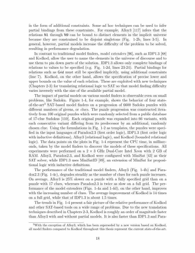
The impact of partial models on various model finders is observable even on smallproblems, like Sudoku. Figure 1-4, for example, shows the behavior of four state-of-the-art3 SAT-based model finders on a progression of 6600 Sudoku puzzles withdifferent numbers of givens, or clues. The puzzle progression was constructed itera-tively from 100 original puzzles which were randomly selected from a public databaseof 17-clue Sudokus [110]. Each original puzzle was expanded into 66 variants, witheach consecutive variant differing from its predecessor by an additional, randomlychosen clue. Using the formulations in Fig. 1-2 as templates, the puzzles were speci-fied in the input languages of Paradox2.3 (first order logic), IDP1.3 (first order logicwith inductive definitions), Alloy3 (relational logic), and Kodkod (bounded relationallogic). The data points on the plots in Fig. 1-4 represent the CPU time, in millisec-onds, taken by the model finders to discover the models of these specifications. Allexperiments were performed on a 2 × 3 GHz Dual-Core Intel Xeon with 2 GB ofRAM. Alloy3, Paradox2.3, and Kodkod were configured with MiniSat [43] as theirSAT solver, while IDP1.3 uses MiniSatID [89], an extension of MiniSat for proposi-tional logic with inductive definitions.

The performance of the traditional model finders, Alloy3 (Fig. 1-4b) and Para-dox2.3 (Fig. 1-4c), degrades steadily as the number of clues for each puzzle increases.On average, Alloy3 is 25% slower on a puzzle with a fully specified grid than on apuzzle with 17 clues, whereaes Paradox2.3 is twice as slow on a full grid. The per-formance of the model extenders (Figs. 1-4a and 1-4d), on the other hand, improveswith the increasing number of clues. The average improvement of Kodkod is 14 timeson a full grid, while that of IDP1.3 is about 1.5 times.

The trends in Fig. 1-4 present a fair picture of the relative performance of Kodkodand other SAT-based tools on a wide range of problems. Due to the new translationtechniques described in Chapters 2-3, Kodkod is roughly an order of magnitude fasterthan Alloy3 with and without partial models. It is also faster than IDP1.3 and Para-

3With the exception of Alloy3, which has been superseded by a new version based on Kodkod,all model finders compared to Kodkod throughout this thesis represent the current state-of-the-art.

18

0

20

40

60

80

100

120

140

10 20 30 40 50 60 70 80 90

milli

seco

nds

number of clues

(a) Kodkod

4200

4400

4600

4800

5000

5200

5400

5600

10 20 30 40 50 60 70 80 90m

illise

cond

snumber of clues

(b) Alloy3

0

50

100

150

200

250

300

10 20 30 40 50 60 70 80 90

milli

seco

nds

number of clues

(c) Paradox2.3

300

350

400

450

500

550

600

10 20 30 40 50 60 70 80 90

milli

seco

nds

number of clues

(d) IDP1.3

Figure 1-4: Effect of partial models on the performance of SAT-based model finders, whenapplied to a progression of 6600 Sudoku puzzles. The x-axis of each graph shows thenumber of clues in a puzzle, and the y-axis shows the time, in milliseconds, taken by a givenmodel finder to solve a puzzle with the specified number of clues. Note that Paradox2.3,IDP1.3 and Kodkod solved many of the puzzles with the same number of clues in the sameamount of time (or within a few milliseconds of one another), so many of the points on theirperformance graphs overlap.

19

0

50

100

150

200

250

300

10 20 30 40 50 60 70 80 90m

illise

cond

snumber of clues

Figure 1-5: Effect of partial models on the performance of a dedicated Sudoku solver, whenapplied to a progression of 6600 Sudoku puzzles.

dox2.3 on the problems that this thesis targets—that is, specifications with partialmodels and intricate constraints over relational structures.4 For a potential user ofthese tools, however, the interesting question is not necessarily how they compare toone another. Rather, the interesting practical question is how they might compare toa custom translation to SAT.

This question is hard to answer in general, but a comparison with existing cus-tom translations is promising. Figure 1-5, for example, shows the performance of adedicated, SAT-based Sudoku solver on the same 6600 puzzles solved with Kodkodand the three other model finders. The solver consists of 150 lines of Java code thatgenerate Lynce and Ouaknine’s optimized SAT encoding [86] of a given Sudoku puz-zle, followed by an invocation of MiniSat on the generated file. The program tooka few hours to write and debug, as the description of the encoding [86] containedseveral errors and ambiguities that had to be resolved during implementation. TheKodkod-based solver, in contrast, consists of about 50 lines of Java API calls thatdirectly correspond to the text in Fig. 1-2a; it took an hour to implement.

The performance of the two solvers, as Figs. 1-4a and 1-5 show, is comparable.The dedicated solver is slightly faster on 17-clue Sudokus, and the Kodkod solveris faster on full grids. The custom solver’s performance remains constant as thenumber of clues in each puzzle increases because it handles the additional clues byfeeding extra unit clauses to the SAT solver: adding these clauses takes negligibletime, and, given that the translation time heavily dominates the SAT solving time,their positive effect on MiniSat’s performance is unobservable. Both implementationswere also applied to 16× 16 and 25× 25 puzzles, with similar outcomes.5 The solversbased on other model finders were unable to solve Sudokus larger than 16× 16.

4Problems that are better suited to other tools than to Kodkod are discussed in Chapter 5.5The bounded relational encoding of Sudoku used in these experiments (Fig. 1-2a) is the easiest

to understand, but it does not produce the most optimal SAT formulas. An alternative encoding,where the multiplicity some on line 10 is replaced by one and each constraint of the form ‘∀ x: ri,y: rj | no (grid[x][y] ∩ grid[ri\x][rj\y])’ is loosened to ‘num ⊆ grid[ri][rj ],’ actually produces a SATencoding that is more efficient than the custom translation across the board. For example, MiniSatsolves the SAT formula corresponding to the alternative encoding of a 64 × 64 Sudoku ten timesfaster than the custom SAT encoding of the same puzzle.

20

1.3 Minimal unsatisfiable core extraction

When a specification has no models in a given universe, most model finders [25, 51,68, 70, 88, 91, 122, 151, 152] simply report that it is unsatisfiable in that universeand offer no further feedback. But many applications need to know the cause of aspecification’s unsatisfiability, either to take corrective action (in the case of declar-ative configuration [133]) or to check that no models exist for the right reasons (inthe case of bounded verification [31, 21]). A bounded verifier [31, 21], for example,checks a system description s1 ∧ . . . ∧ sn against a property p in some finite universeby looking for models of the formula s1∧ . . .∧ sn∧¬p in that universe. If found, sucha model, or a counterexample, represents a behavior of the system that violates p. Alack of models, however, does not necessarily mean that the analysis was successful.If no models exist because the system description is overconstrained, or because theproperty is a tautology, the analysis is considered to have failed due to a vacuity error.

A cause of unsatisfiability of a given specification, expressed as a subset of thespecification’s constraints that is itself unsatisfiable, is called an unsatisfiable core.Every unsatisfiable core includes one or more critical constraints that cannot be re-moved without making the remainder of the core satisfiable. Non-critical constraints,if any, are irrelevant to unsatisfiability and generally decrease a core’s utility bothfor diagnosing faulty configurations [133] and for checking the results of a boundedanalysis [129]. Cores that include only critical constraints are said to be minimal.

3 8

2 4 1 9 6

1 8 9 3 5

6 9 1

3 9 7

3 5 8

1 9

8 9 4 5 6

3 5 6 4 2

(a) An unsatisfiable Sudoku puzzle

1 {1, 2, 3, 4, 5, 6, 7, 8, 9}

2 num :1 [{〈1〉,〈2〉,〈3〉,〈4〉,〈5〉,〈6〉,〈7〉,〈8〉,〈9〉},3 {〈1〉,〈2〉,〈3〉,〈4〉,〈5〉,〈6〉,〈7〉,〈8〉,〈9〉}]4 r1 :1 [{〈1〉,〈2〉,〈3〉}, {〈1〉,〈2〉,〈3〉}]5 r2 :1 [{〈4〉,〈5〉,〈6〉}, {〈4〉,〈5〉,〈6〉}]6 r3 :1 [{〈7〉,〈8〉,〈9〉}, {〈7〉,〈8〉,〈9〉}]7 grid :3 [{〈1, 6, 3〉,〈1, 9, 8〉, . . . , 〈9, 9, 2〉},8 {〈1, 1, 1〉, . . . , 〈1, 5, 9〉, 〈1, 6, 3〉,9 〈1, 7, 1〉,〈1, 7, 2〉, . . . , 〈9, 9, 2〉}]

10 ∀ x, y: num | some grid[x][y]11 ∀ x, y: num | no (grid[x][y] ∩ grid[x][num\y])12 ∀ x, y: num | no (grid[x][y] ∩ grid[num\x][y])13 ∀ x: r1, y: r1 | no (grid[x][y] ∩ grid[r1\x][r1\y])14 ∀ x: r1, y: r3 | no (grid[x][y] ∩ grid[r1\x][r3\y])15 ∀ x: r1, y: r2 | no (grid[x][y] ∩ grid[r1\x][r2\y])16 ∀ x: r2, y: r1 | no (grid[x][y] ∩ grid[r2\x][r1\y])17 ∀ x: r2, y: r2 | no (grid[x][y] ∩ grid[r2\x][r2\y])18 ∀ x: r2, y: r3 | no (grid[x][y] ∩ grid[r2\x][r3\y])19 ∀ x: r3, y: r1 | no (grid[x][y] ∩ grid[r3\x][r1\y])20 ∀ x: r3, y: r2 | no (grid[x][y] ∩ grid[r3\x][r2\y])21 ∀ x: r3, y: r3 | no (grid[x][y] ∩ grid[r3\x][r3\y])

(b) Core of the puzzle (highlighted)

Figure 1-6: An unsatisfiable Sudoku puzzle and its core.

Figure 1-6 shows an example of using a minimal core to diagnose a faulty Sudokuconfiguration. The highlighted parts of Fig. 1-6b comprise a set of critical constraints

21

that cannot be satisfied by the puzzle in Fig. 1-6a. The row (line 11) and column (line12) constraints rule out ‘9’ as a valid value for any of the blank cells in the bottomright region. The values ‘2’, ‘4’, and ‘6’ are also ruled out (line 21), leaving five uniquenumbers and six empty cells. By the pigeonhole principle, these cells cannot be filled(as required by line 10) without repeating some value (which is disallowed by line21). Removing ‘2’ from the highlighted cell fixes the puzzle.

The problem of unsatisfiable core extraction has been studied extensively in theSAT community, and there are many efficient algorithms for finding small or minimalcores of propositional formulas [32, 60, 61, 59, 79, 85, 97, 102, 153]. A simple facilityfor leveraging these algorithms in the context of SAT-based model finding has beenimplemented as a feature of Alloy3. The underlying mechanism [118] involves trans-lating a specification to a SAT problem; finding a core of the translation using anexisting SAT-level algorithm [153]; and mapping the clauses from the boolean coreback to the specification constraints from which they were generated. The resultingspecification-level core is guaranteed to be sound (i.e. unsatisfiable) [118], but it isnot guaranteed to be minimal or even small.

Recycling core extraction (RCE) is a new SAT-based algorithm for finding coresof declarative specifications that are both sound and minimal. It has two key ideas(Chapter 4). The first idea is to lift the minimization process from the boolean levelto the specification level. Instead of attempting to minimize the boolean core, RCEmaps it back and then minimizes the resulting specification-level core, by removingcandidate constraints and testing the remainder for satisfiability. The second idea isto use the proof of unsatisfiability returned by the SAT solver, and the mapping be-tween the specification constraints and the translation clauses, to identify the booleanclauses that were inferred by the solver and that still hold when a specification-levelconstraint is removed. By adding these clauses to the translation of a candidate core,RCE allows the solver to reuse previously made inferences.

Both ideas employed by RCE are straightforward and relatively easy to imple-ment, but have dramatic consequences on the quality of the results obtained and theperformance of the analysis. Compared to NCE and SCE [129], two variants of RCEthat lack some of its optimizations, RCE is roughly 20 to 30 times faster on hardproblems and 10 to 60 percent faster on easier problems (Chapter 4). It is muchslower than Alloy3’s core extractor, OCE [118], which does not guarantee minimal-ity. Most cores produced by OCE, however, include large proportions of irrelevantconstraints, making them hard to use in practice.

Figure 1-7, for example, compares RCE with OCE, NCE and SCE on a set of100 unsatisfiable Sudokus. The puzzles were constructed from 100 randomly selected16 × 16 Sudokus [63], each of which was augmented with a randomly chosen, faultyclue. Figure 1-7a shows the number of puzzles on which RCE is faster (or slower)than each competing algorithm by a factor that falls within the given range. Figure1-7b shows the number of puzzles whose RCE cores are smaller (or larger) than thoseof the competing algorithms by a factor that falls within the given range. All fourextractors were implemented in Kodkod, configured with MiniSat, and all experimentswere performed on a 2× 3 GHz Dual-Core Intel Xeon with 2 GB of RAM.

Because SCE is essentially RCE without the clause recycling optimization, they

22

1

3

10

32

100

(0, 0.1] (0.1, 0.5] (0.5, 1] (1, 2] (2, 16]

20

56

910

5

14

71

15

100

# o

f p

uzzle

s

extraction time ratio

OCE/RCESCE/RCENCE/RCE

0.20

0.04

0.72

0.02

0.89

1.211.44

2.744.40

(a) Extraction times

1

3

10

32

100

(0, 1) [1, 1] (1, 1.5] (1.5, 2] (2, 5]

6

20

69

56

92

2

17

58

21

4# o

f p

uzzle

s

core size ratio

OCE/RCESCE/RCENCE/RCE

1.00

1.001.00

0.90

0.79

1.32

1.20

1.28

1.76

1.73

2.84

(b) Core sizes

Figure 1-7: Comparison of SAT-based core extractors on 100 unsatisfiable Sudokus. Figure(a) shows the number of puzzles on which RCE is faster, or slower, than each competingalgorithm by a factor that falls within the given range. Figure (b) shows the number ofpuzzles whose RCE cores are smaller, or larger, than those of the competing algorithmsby a factor that falls within the given range. Both histograms are shown on a logarithmicscale. The number above each column specifies its height, and the middle number is theaverage extraction time (or core size) ratio for the puzzles in the given category.

23

usually end up finding the same minimal core. Of the 100 cores extracted by eachalgorithm, 92 were the same (Fig. 1-7b). RCE was faster than SCE on 85 of theproblems (Fig. 1-7a). Since Sudoku cores are easy to find6, the average speed up ofRCE over SCE is about 37%. NCE is the most naive of the three approaches and doesnot exploit the boolean-level cores in any way. It found a different minimal core thanRCE for 31 of the puzzles. For 26 of those, the NCE core was larger than the RCEcore, and indeed, easier to find, as shown in Fig. 1-7a. Nonetheless, RCE was, onaverage, 77% faster than NCE. OCE outperformed all three minimality-guaranteeingalgorithms by large margins. However, only four OCE cores were minimal, and morethan half the constraints in 75 of its cores were irrelevant.

1.4 Summary of contributions

This thesis contributes a collection of techniques (Fig. 1-8) that enable easy andefficient use of SAT for declarative problem solving. They include:

1. A new problem-description language that extends the relational logic of Al-loy [69] with a mechanism for specifying precise bounds on the values of freevariables (Chapter 2); the bounds enable efficient encoding and exploitation ofpartial models.

2. A new translation to SAT that uses sparse-matrices and auto-compacting cir-cuits (Chapter 2); the resulting boolean encoding is significantly smaller, fasterto produce, and easier to solve than the encodings obtained with previouslypublished techniques [40, 119].

3. A new algorithm for identifying symmetries that works in the presence of arbi-trary bounds on free variables (Chapter 3); the algorithm employs a fast greedytechnique that is both effective in practice and scales better than a completemethod based on graph automorphism detection.

4. A new algorithm for finding minimal unsatisfiable cores that recycles infer-ences made at the boolean level to speed up core extraction at the specificationlevel (Chapter 4); the algorithm is much faster on hard problems than relatedapproaches [129], and its cores are much smaller than those obtained with non-minimal extractors [118].

These techniques have been prototyped in Kodkod, a new engine for finding mod-els and cores of large relational specifications. The engine significantly outperformsexisting model finders [13, 25, 88, 93, 117, 152] on problems with partial models,rich type hierarchies, and low-arity relations. As such problems arise in a widerange of declarative configuration and analysis settings, Kodkod has been used inseveral configuration [149, 101], test-case generation [114, 135] and bounded verifi-cation [21, 137, 31, 126, 34] tools (Table 1.1). These applications have served as a

6Chapter 4 describes a metric for approximating the difficulty of a given problem for a particularcore extraction algorithm.

24

relationalspecification

relational bounds

universe of discourse

skolemizer

symmetrydetector

symmetrybreaker

skolemizedspecification

universepartitioning

circuit transformer

translationcircuit

symmetry-breaking circuit

sparse-matrix translator

SAT solver

CNF modelauto-compact. circuit factory

sat?

core extractor

unsat?

minimal core

Chapter 3

Chapter 2

Chapter 4

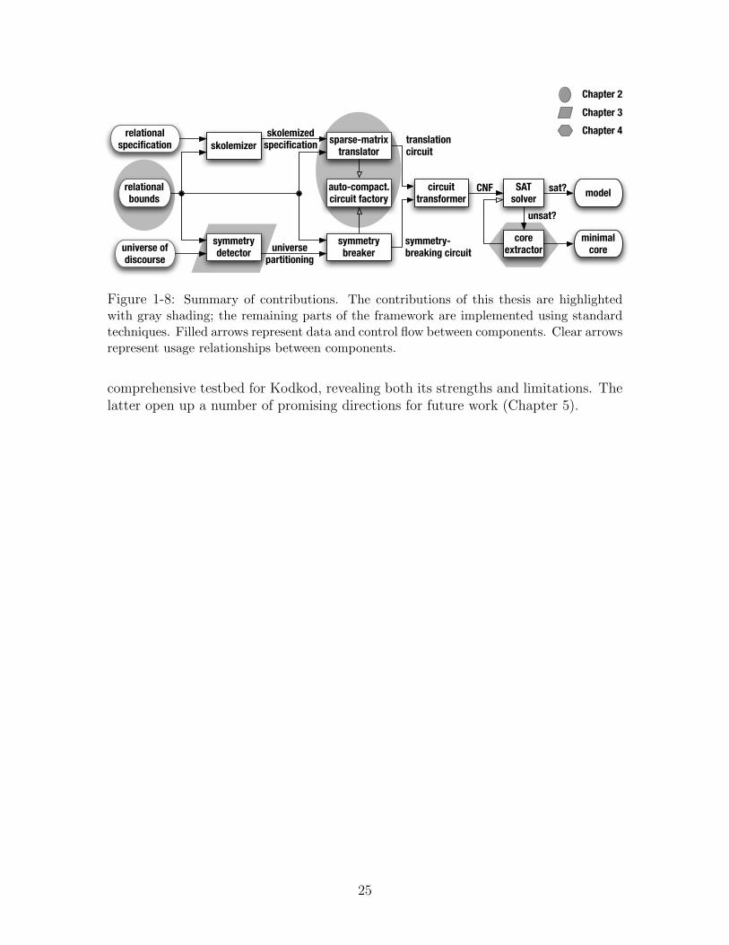
Figure 1-8: Summary of contributions. The contributions of this thesis are highlightedwith gray shading; the remaining parts of the framework are implemented using standardtechniques. Filled arrows represent data and control flow between components. Clear arrowsrepresent usage relationships between components.

comprehensive testbed for Kodkod, revealing both its strengths and limitations. Thelatter open up a number of promising directions for future work (Chapter 5).

25

bou

nded

veri

fica

tion

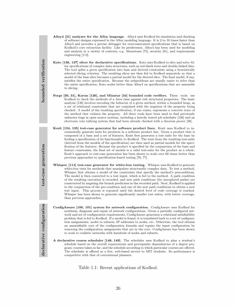
Alloy4 [21] analyzer for the Alloy language. Alloy4 uses Kodkod for simulation and checkingof software designs expressed in the Alloy modeling language. It is 2 to 10 times faster thanAlloy3 and provides a precise debugger for overconstrained specifications that is based onKodkod’s core extraction facility. Like its predecessor, Alloy4 has been used for modelingand analysis in a variety of contexts, e.g. filesystems [75], security [81], and requirementsengineering [113].

Kato [136, 137] slicer for declarative specifications. Kato uses Kodkod to slice and solve Al-loy specifications of complex data structures, such as red-black trees and doubly-linked lists.The tool splits a given specification into base and derived constraints using a heuristicallyselected slicing criterion. The resulting slices are then fed to Kodkod separately so that amodel of the base slice becomes a partial model for the derived slice. The final model, if any,satisfies the entire specification. Because the subproblems are usually easier to solve thanthe entire specification, Kato scales better than Alloy4 on specifications that are amenableto slicing.

Forge [30, 31], Karun [126], and Minatur [34] bounded code verifiers. These tools useKodkod to check the methods of a Java class against rich structural properties. The basicanalysis [138] involves encoding the behavior of a given method, within a bounded heap, asa set of relational constraints that are conjoined with the negation of the property beingchecked. A model of the resulting specification, if one exists, represents a concrete trace ofthe method that violates the property. All three tools have been used to find previouslyunknown bugs in open source systems, including a heavily tested job scheduler [126] and anelectronic vote tallying system that had been already checked with a theorem prover [30].

test

-cas

ege

ner

atio

n

Kesit [134, 135] test-case generator for software product lines. Kesit uses Kodkod to in-crementally generate tests for products in a software product line. Given a product that iscomposed of a base and a set of features, Kesit first generates a test suite for the base byfeeding a specification of its functionality to Kodkod. The tests from the resulting test-suite(derived from the models of the specification) are then used as partial models for the speci-fication of the features. Because the product is specified by the conjunction of the base andfeature constraints, the final set of models is a valid test-suite for the product as a whole.Kesit’s approach to test-case generation has been shown to scale over 60 times better thanprevious approaches to specification-based testing [76, 77].

Whispec [114] test-case generator for white-box testing. Whispec uses Kodkod to generatewhite-box tests for methods that manipulate structurally complex data. To test a method,Whispec first obtains a model of the constraints that specify the method’s preconditions.The model is then converted to a test input, which is fed to the method. A path conditionof the resulting execution is recorded, and new path conditions (for unexplored paths) areconstructed by negating the branch predicates in the recorded path. Next, Kodkod is appliedto the conjunction of the pre-condition and one of the new path conditions to obtain a newtest input. This process is repeated until the desired level of code coverage is reached.Whispec has been shown to generate significantly smaller test suites, with better coverage,than previous approaches.

dec

lara

tive

configu

rati

on ConfigAssure [100, 101] system for network configuration. ConfigAssure uses Kodkod forsynthesis, diagnosis and repair of network configurations. Given a partially configured net-work and set of configuration requirements, ConfigAssure generates a relational satisfiabilityproblem that is fed to Kodkod. If a model is found, it is translated back to a set of configura-tion assignments: nodes to subnets, IP addresses to nodes, etc. Otherwise, the tool obtainsan unsatisfiable core of the configuration formula and repairs the input configuration byremoving the configuration assignments that are in the core. ConfigAssure has been shownto scale to realistic networks with hundreds of nodes and subnets.

A declarative course scheduler [148, 149]. The scheduler uses Kodkod to plan a student’sschedule based on the overall requirements and prerequisite dependencies of a degree pro-gram; courses taken so far; and the schedule according to which particular courses are offered.The scheduler is offered as a free, web-based service to MIT students. Its performance iscompetitive with that of conventional planners.

Table 1.1: Recent applications of Kodkod.

26

Chapter 2

From Relational to Boolean Logic

The relational logic of Alloy [69] combines the quantifiers of first order logic withthe operators of relational algebra. The logic and the language were designed formodeling software abstractions, their properties and invariants. But unlike the logicsof traditional modeling languages [123, 143], Alloy makes no distinction betweenrelations, sets and scalars: sets are relations with one column, and scalars are singletonsets. Treating everything as a relation makes the logic more uniform and, in someways, easier to use than traditional modeling languages. Applying a partial functionoutside of its domain, for example, simply yields the empty set, eliminating the needfor special undefined values.

The generality and versatility of Alloy’s logic have prompted several attempts touse its model finder, Alloy3 [117], as a generic constraint solving engine for declarativeconfiguration [99] and analysis [76, 138]. These efforts, however, were hampered bytwo key limitations of the Alloy system. First, Alloy has no notion of a partial model.If a partial solution, or a model, is available for a set of Alloy constraints, it canonly be provided to the solver in the form of additional constraints. Because thesolver is essentially forced to rediscover the partial model from the constraints, thisstrategy does not scale well in practice. Second, Alloy3 was designed for small-scopeanalysis [69] of hand-crafted specifications of software systems, so it performs poorlyon problems with large universes or large, automatically generated specifications.

Kodkod is a new tool that is designed for use as a generic relational engine.Its model finder, like Alloy3, works by translating relational to boolean logic andapplying an off-the-shelf SAT solver to the resulting boolean formula. Unlike Alloy3,however, Kodkod scales in the presence of partial models, and it can handle largeuniverses and specifications. This chapter describes the elements of Kodkod’s logicand model finder that are key to its ability to produce compact SAT formulas, withand without partial models. Next chapter describes a technique that is used formaking the produced formulas slightly larger but easier to solve.

27

2.1 Bounded relational logic

A specification in the relational logic of Alloy is a collection of constraints on a set ofrelational variables. A model of an Alloy specification is a binding of its free variablesto relational constants that makes the specification true. These constants are setsof tuples, drawn from a common universe of uninterpreted elements, or atoms. Theuniverse itself is implicit, in the sense that its elements cannot be named or referencedthrough any syntactic construct of the logic. As a result, there is no direct way tospecify relational constants in Alloy. If a partial binding of relations to constants—i.e. a partial model—is available for a specification, it must be encoded indirectly,with constraints that use additional variables (e.g. N1 through N9 in Fig. 1-2b) asimplicit handles to distinct atoms. While sound, this encoding of partial models isimpractical because the additional variables and constraints make the resulting modelfinding problem larger rather than smaller.

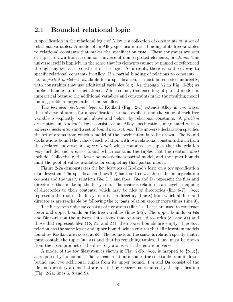
The bounded relational logic of Kodkod (Fig. 2-1) extends Alloy in two ways:the universe of atoms for a specification is made explicit, and the value of each freevariable is explicitly bound, above and below, by relational constants. A problemdescription in Kodkod’s logic consists of an Alloy specification, augmented with auniverse declaration and a set of bound declarations. The universe declaration specifiesthe set of atoms from which a model of the specification is to be drawn. The bounddeclarations bound the value of each relation with two relational constants drawn fromthe declared universe: an upper bound, which contains the tuples that the relationmay include, and a lower bound, which contains the tuples that the relation mustinclude. Collectively, the lower bounds define a partial model, and the upper boundslimit the pool of values available for completing that partial model.

Figure 2-2a demonstrates the key features of Kodkod’s logic on a toy specificationof a filesystem. The specification (lines 6-9) has four free variables: the binary relationcontents and the unary relations File, Dir, and Root. File and Dir represent the files anddirectories that make up the filesystem. The contents relation is an acyclic mappingof directories to their contents, which may be files or directories (line 6-7). Root

represents the root of the filesystem: it is a directory (line 8) from which all files anddirectories are reachable by following the contents relation zero or more times (line 9).

The filesystem universe consists of five atoms (line 1). These are used to constructlower and upper bounds on the free variables (lines 2-5). The upper bounds on File

and Dir partition the universe into atoms that represent directories (d0 and d1) andthose that represent files (f0, f1, and f2); their lower bounds are empty. The Root

relation has the same lower and upper bound, which ensures that all filesystem modelsfound by Kodkod are rooted at d0. The bounds on the contents relation specify that itmust contain the tuple 〈d0, d1〉 and that its remaining tuples, if any, must be drawnfrom the cross product of the directory atoms with the entire universe.

A model of the toy filesystem is shown in Fig. 2-2b. Root is mapped to {〈d0〉},as required by its bounds. The contents relation includes the sole tuple from its lowerbound and two additional tuples from its upper bound. File and Dir consist of thefile and directory atoms that are related by contents, as required by the specification(Fig. 2-2a, lines 6, 8 and 9).

28

problem := universe relBound∗ formula∗

universe := { atom[, atom]∗ }relBound := var :arity [[constant, constant]]constant := {tuple[, tuple]∗} | {}[×{}]∗tuple := 〈atom[, atom]∗〉

atom, var := identifierarity := positive integer

formula :=no expr empty| lone expr at most one| one expr exactly one| some expr non-empty| expr ⊆ expr subset| expr = expr equal| ¬ formula negation| formula ∧ formula conjunction| formula ∨ formula disjunction| formula ⇒ formula implication| formula ⇔ formula equivalence

| ∀ varDecls || formula universal

| ∃ varDecls || formula existential

expr :=var variable| expr transpose| expr closure

| ∗expr reflex. closure| expr ∪ expr union| expr ∩ expr intersection| expr \ expr difference| expr . expr join

| expr → expr product

| formula ? expr : expr if-then-else

| {varDecls || formula} comprehension

varDecls := var : expr[, var : expr]∗

(a) Abstract syntax

P : problem → binding → booleanR : relBound → binding → booleanF : formula → binding → booleanE : expr → binding → constantbinding : var → constant

PJ{a1, . . . , an} r1 . . . rj f1 . . . fmKb :=RJr1Kb ∧ . . .∧ RJrjKb ∧ FJf1Kb ∧ . . .∧ FJfmKb

RJv :k [l, u]Kb := l ⊆ b(v) ⊆ u

FJno pKb := |EJpKb| = 0FJlone pKb := |EJpKb| ≤ 1FJone pKb := |EJpKb| = 1FJsome pKb := |EJpKb| > 0FJp ⊆ qKb := EJpKb ⊆ EJqKbFJp = qKb := EJpKb = EJqKbFJ¬fKb := ¬FJfKbFJf ∧ gKb := FJfKb ∧ FJgKbFJf ∨ gKb := FJfKb ∨ FJgKbFJf ⇒ gKb := FJfKb⇒ FJgKbFJf ⇔ gKb := FJfKb⇔ FJgKb

FJ∀ v1 : e1, ..., vn : en || fKb :=Vs∈EJe1Kb(FJ∀ v2 : e2, ..., vn : en || fK(b⊕ v1 7→{〈s〉})

FJ∃ v1 : e1, ..., vn : en || fKb :=Ws∈EJe1Kb(FJ∃ v2 : e2, ..., vn : en || fK(b⊕ v1 7→{〈s〉})

EJvKb := b(v)EJ pKb := {〈p2, p1〉 | 〈p1, p2〉 ∈ EJpKb}EJ pKb := {〈p1, pn〉 | ∃ p2, ..., pn−1 |

〈p1, p2〉, ..., 〈pn−1, pn〉 ∈ EJpKb}EJ∗pKb := EJ pKb ∪ {〈p1, p1〉 | true}EJp ∪ qKb := EJpKb ∪ EJqKbEJp ∩ qKb := EJpKb ∩ EJqKbEJp \ qKb := EJpKb \ EJqKbEJp . qKb := {〈p1, ..., pn−1, q2, ..., qm〉 | 〈p1, ..., pn〉

∈ EJpKb ∧ 〈q1, ..., qm〉 ∈ EJqKb }EJp→qKb := {〈p1, ..., pn, q1, ..., qm〉 | 〈p1, ..., pn〉

∈ EJpKb ∧ 〈q1, ..., qm〉 ∈ EJqKb }EJf ? p : qKb := if FJfKb then EJpKb else EJqKb

EJ{v1 : e1, ..., vn : en || f}Kb :={〈s1, ..., sn〉 | s1∈EJe1Kb ∧ s2∈EJe2K(b⊕ v1 7→{〈s1〉})∧ . . . ∧ sn∈EJenK(b⊕

Sn−1i=1 vi 7→{〈si〉})

∧FJfK(b⊕Sn

i=1 vi 7→{〈si〉})}

(b) Semantics

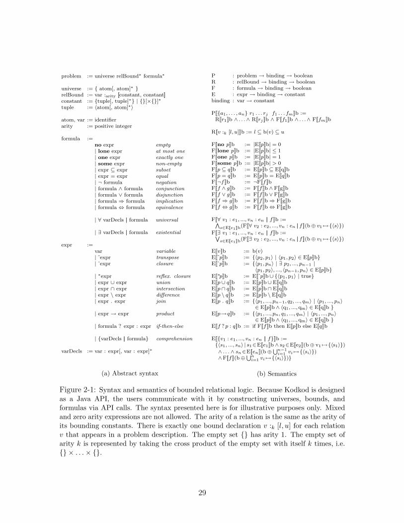
Figure 2-1: Syntax and semantics of bounded relational logic. Because Kodkod is designedas a Java API, the users communicate with it by constructing universes, bounds, andformulas via API calls. The syntax presented here is for illustrative purposes only. Mixedand zero arity expressions are not allowed. The arity of a relation is the same as the arity ofits bounding constants. There is exactly one bound declaration v :k [l, u] for each relationv that appears in a problem description. The empty set {} has arity 1. The empty set ofarity k is represented by taking the cross product of the empty set with itself k times, i.e.{} × . . .× {}.

29

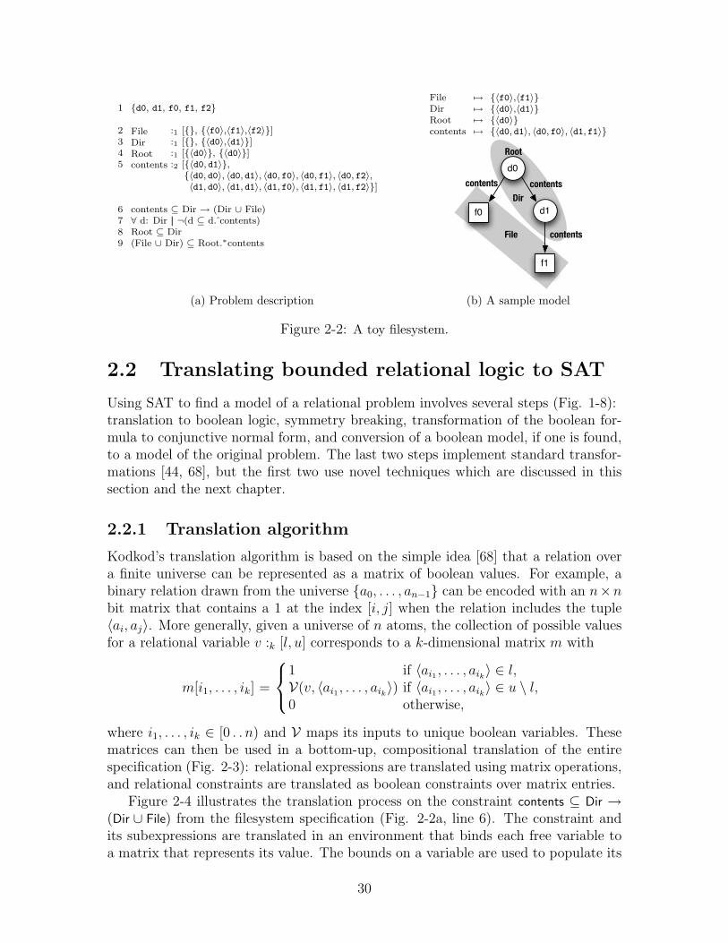
1 {d0, d1, f0, f1, f2}

2 File :1 [{}, {〈f0〉,〈f1〉,〈f2〉}]3 Dir :1 [{}, {〈d0〉,〈d1〉}]4 Root :1 [{〈d0〉}, {〈d0〉}]5 contents :2 [{〈d0, d1〉},

{〈d0, d0〉, 〈d0, d1〉, 〈d0, f0〉, 〈d0, f1〉, 〈d0, f2〉,〈d1, d0〉, 〈d1, d1〉, 〈d1, f0〉, 〈d1, f1〉, 〈d1, f2〉}]

6 contents ⊆ Dir → (Dir ∪ File)7 ∀ d: Dir || ¬(d ⊆ d. contents)8 Root ⊆ Dir9 (File ∪ Dir) ⊆ Root.∗contents

(a) Problem description

File 7→ {〈f0〉,〈f1〉}Dir 7→ {〈d0〉,〈d1〉}Root 7→ {〈d0〉}contents 7→ {〈d0, d1〉, 〈d0, f0〉, 〈d1, f1〉}

d0

d1f0

f1

contentscontents

contents

Root

Dir

File

(b) A sample model

Figure 2-2: A toy filesystem.

2.2 Translating bounded relational logic to SAT

Using SAT to find a model of a relational problem involves several steps (Fig. 1-8):translation to boolean logic, symmetry breaking, transformation of the boolean for-mula to conjunctive normal form, and conversion of a boolean model, if one is found,to a model of the original problem. The last two steps implement standard transfor-mations [44, 68], but the first two use novel techniques which are discussed in thissection and the next chapter.

2.2.1 Translation algorithm

Kodkod’s translation algorithm is based on the simple idea [68] that a relation overa finite universe can be represented as a matrix of boolean values. For example, abinary relation drawn from the universe {a0, . . . , an−1} can be encoded with an n×nbit matrix that contains a 1 at the index [i, j] when the relation includes the tuple〈ai, aj〉. More generally, given a universe of n atoms, the collection of possible valuesfor a relational variable v :k [l, u] corresponds to a k-dimensional matrix m with

m[i1, . . . , ik] =

1 if 〈ai1 , . . . , aik〉 ∈ l,V(v, 〈ai1 , . . . , aik〉) if 〈ai1 , . . . , aik〉 ∈ u \ l,0 otherwise,

where i1, . . . , ik ∈ [0 . . n) and V maps its inputs to unique boolean variables. Thesematrices can then be used in a bottom-up, compositional translation of the entirespecification (Fig. 2-3): relational expressions are translated using matrix operations,and relational constraints are translated as boolean constraints over matrix entries.

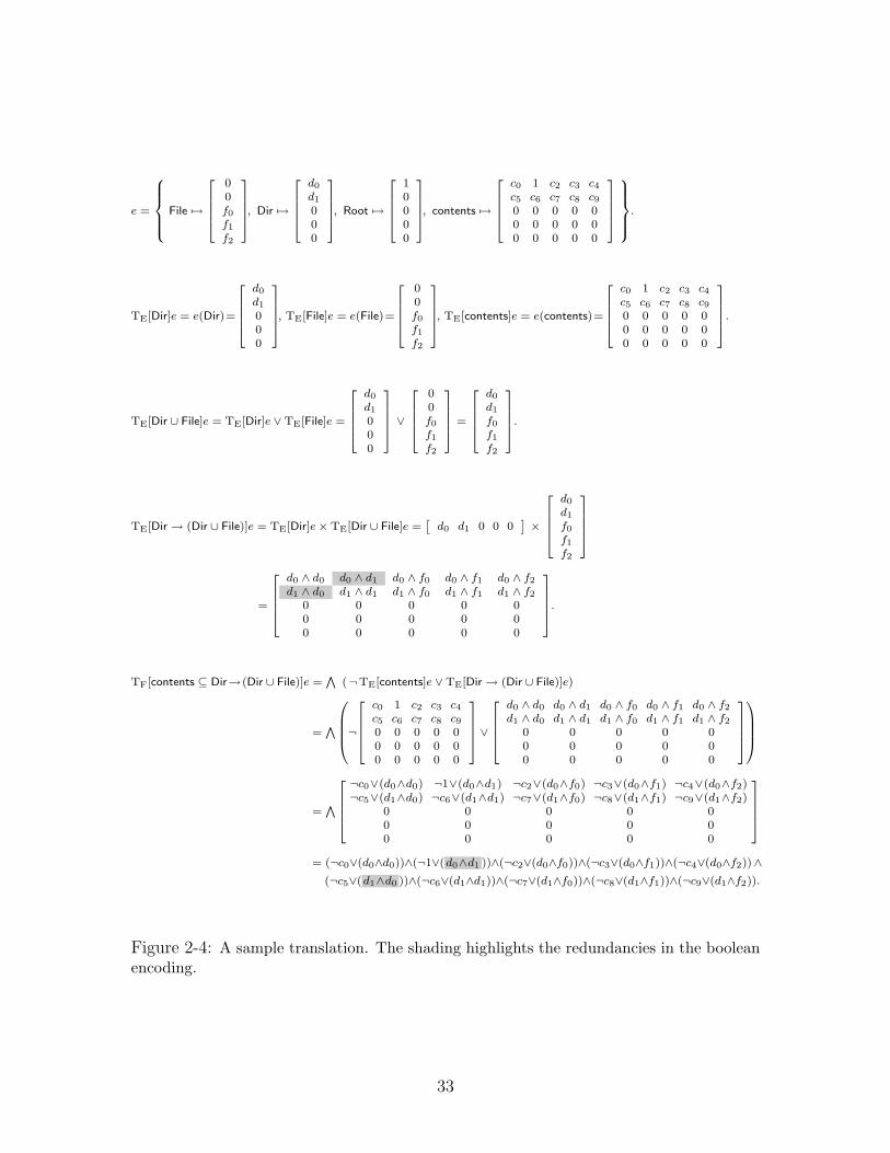
Figure 2-4 illustrates the translation process on the constraint contents ⊆ Dir →(Dir ∪ File) from the filesystem specification (Fig. 2-2a, line 6). The constraint andits subexpressions are translated in an environment that binds each free variable toa matrix that represents its value. The bounds on a variable are used to populate its

30

TP : problem → bool

TR : relBound → universe → matrix

TF : formula → env → boolTE : expr → env → matrix

env : var → matrix

bool := 0 | 1 | boolVar | ¬ bool | bool ∧ bool | bool ∨ bool | bool ? bool : boolboolVar := identifier

idx := 〈int[, int]∗〉

V : var → 〈atom[, atom]∗〉 → boolVar boolean variable for a given tuple in a relationL M : matrix → {idx[, idx]∗} set of all indices in a matrix

J K : matrix → intint size of a matrix, (size of a dimension)number of dimensions

[ ] : matrix → idx → bool matrix value at a given index

M : intint → (idx → bool) → matrixM(sd, f) := new m ∈ matrix where JmK = sd ∧ ∀ ~x ∈ {0, ..., s− 1}d, m[~x] = f(~x)

M : intint → idx → matrixM(sd, ~x) := M(sd, λ~y. if ~y = ~x then 1 else 0)

TP[{a1, . . . , an} v1 :k1[l1, u1] . . . vj :kj[lj , uj ] f1 . . . fm] := TF[

Vmi=1 fi](∪j

i=1vi 7→ TR[vi :ki[li, ui], {a1, . . . , an}])

TR[v :k [l, u], {a1, . . . , an}] := M(nk, λ〈i1, ...ik〉. if 〈ai1 , . . . , aik〉 ∈ l then 1

else if 〈ai1 , . . . , aik〉 ∈ u \ l then V(v, 〈ai1 , . . . , aik

〉)else 0)

TF[no p]e := ¬TF[some p]e

TF[lone p]e := TF[no p]e ∨ TF[one p]e

TF[one p]e := let m← TE[p]e inW

~x∈LmM m[~x] ∧ (V

~y∈LmM\{~x} ¬m[~y])

TF[some p]e := let m← TE[p]e inW

~x∈LmM m[~x]

TF[p ⊆ q]e := let m← (¬TE[p]e ∨ TE[q]e) inV

~x∈LmM m[~x]

TF[p = q]e := TF[p ⊆ q]e ∧ TF[q ⊆ p]e

TF[not f ]e := ¬TF[f ]e

TF[f ∧ g]e := TF[f ]e ∧ TF[g]eTF[f ∨ g]e := TF[f ]e ∨ TF[g]e

TF[f ⇒ g]e := ¬TF[f ]e ∨ TF[g]e

TF[f ⇔ g]e := (TF[f ]e ∧ TF[g]e) ∨ (¬TF[f ]e ∧ ¬TF[g]e)

TF[∀ v1 : e1, ..., vn : en || f ]e := let m← TE[e1]e inV

~x∈LmM(¬m[~x]∨TF[∀ v2 : e2, ..., vn : en || f ](e⊕v1 7→ M(JmK, ~x)))

TF[∃ v1 : e1, ..., vn : en || f ]e := let m← TE[e1]e inW

~x∈LmM(m[~x] ∧ TF[∀ v2 : e2, ..., vn : en || f ](e⊕ v1 7→ M(JmK, ~x)))

TE[v]e := e(v)TE [ p]e := (TE[p]e)T

TE [ p]e := let m← TE[p]e, sd ← JmK, sq← (λx.i. if i=s then x else let y←sq(x, i ∗ 2) in y ∨ y · y) in sq(m, 1)

TE[∗p]e := let m← TE [ p]e, sd ← JmK in m ∨M(sd, λ〈i1, . . . , id〉. if i1 = i2 ∧ . . . ∧ i1 = ik then 1 else 0)

TE[p ∪ q]e := TE[p]e ∨ TE[q]eTE[p ∩ q]e := TE[p]e ∧ TE[q]eTE[p \ q]e := TE[p]e ∧ ¬TE[q]eTE[p . q]e := TE[p]e · TE[q]eTE[p→q]e := TE[p]e× TE[q]e

TE[f ? p : q]e := let mp ← TE[p]e, mp ← TE[q]e inM(JmpK, λ~x. TF[f ]e ? mp[~x] : mq [~x])

TE[{v1 : e1, ..., vn : en || f}]e := let m1 ← TE[e1]e, sd ← Jm1K in

M(sn, λ〈i1, . . . , in〉. let m2 ← TE[e2](e⊕ v1 7→ M(s, 〈i1〉)), . . . ,mn ← TE[en](e⊕ v1 7→ M(s, 〈i1〉)⊕ . . .⊕ vn−1 7→ M(s, 〈in−1〉)) inm1[i1] ∧ . . . ∧mn[in] ∧ TF[f ](e⊕ v1 7→ M(s, 〈i1〉)⊕ . . .⊕ vn 7→ M(s, 〈in〉)))

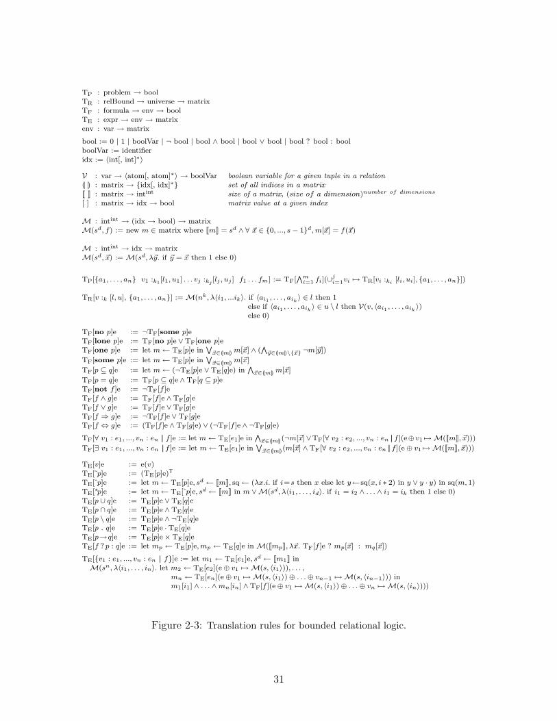
Figure 2-3: Translation rules for bounded relational logic.

31

representation matrix as follows: lower bound tuples are represented with 1s in thecorresponding matrix entries; tuples that are in the upper but not the lower boundare represented with fresh boolean variables; and tuples outside the upper bound arerepresented with 0s. Translation of the remaining expressions is straightforward. Theunion of Dir and File is translated as the disjunction of their translations so that a tupleis in Dir ∪ File if it is in Dir or File; relational cross product becomes the generalizedcross product of matrices, with conjunction used instead of multiplication; and thesubset constraint forces each boolean variable representing a tuple in Dir→ (Dir∪File)to evaluate to 1 whenever the boolean representation of the corresponding tuple inthe contents relation evaluates to the same.

2.2.2 Sparse-matrix representation of relations

Many problems suitable for solving with a relational engine are typed: their uni-verses are partitioned into sets of atoms according to a type hierarchy, and theirexpressions are bounded above by relations over these sets [39]. The toy filesys-tem, for example, is defined over a universe that consists of two types of atoms:the atoms that represent directories and those that represent files. Each expres-sion in the filesystem specification (Fig. 2-2a) is bounded above by a relation overthe types Tdir = {d0, d1} and Tfile = {f0, f1, f2}. The upper bound on contents,for example, relates the directory type to both the directory and file types, i.e.dcontentse = {〈Tdir, Tdir〉, 〈Tdir, Tfile〉} = {d0, d1} × {d0, d1} ∪ {d0, d1} × {f0, f1, f2}.

Previous relational engines (§2.3.1) employed a type checker [39, 128], a source-to-source transformation [40], and a typed translation [68, 117], in an effort to reduce thenumber of boolean variables used to encode typed problems. Kodkod’s translation,on the other hand, is designed to exploit types, provided as upper bounds on freevariables, transparently: each relational variable is represented as an untyped matrixwhose dimensions correspond to the entire universe, but the entries outside the vari-able’s upper bound are zeroed out. The zeros are then propagated up the translationchain, ensuring that no boolean variables are wasted on tuples guaranteed to be out-side an expression’s valuation. The upper bound on the expression Dir→ (Dir∪ File),for example, is {〈Tdir, Tdir〉, 〈Tdir, Tfile〉}, and the regions of its translation matrix (Fig.2-4) that correspond to the tuples outside of its ‘type’ are zeroed out.

This simple scheme for exploiting both types and partial models is enabled bya new multidimensional sparse-matrix data structure for representing relations. Asnoted in previous work [40], an untyped translation algorithm cannot scale if based onthe standard encoding of matrices as multi-dimensional arrays, because the numberof zeros in a k-dimensional matrix over a universe of n atoms grows proportionallyto nk. Kodkod therefore encodes translation matrices as balanced trees that storeonly non-zero values. In particular, each tree node corresponds to a non-zero cell (ora range of cells) in the full nk matrix. The cell at the index [i1, . . . , ik] that storesthe value v becomes a node with

∑kj=1 ijn

k−j as its key and v as its value, wherethe index-to-key conversion yields the decimal representation of the n-ary numberi1 . . . ik. Nodes with consecutive keys that store a 1 are merged into a single nodewith a range of keys, enabling compact representation of lower bounds.

32

e =

8>>><>>>: File 7→

2666400f0

f1

f2

37775, Dir 7→

26664d0

d1

000

37775, Root 7→

2666410000

37775, contents 7→

26664c0 1 c2 c3 c4c5 c6 c7 c8 c90 0 0 0 00 0 0 0 00 0 0 0 0

377759>>>=>>>;.

TE[Dir]e = e(Dir)=

26664d0

d1

000

37775, TE[File]e = e(File)=

2666400f0

f1

f2

37775, TE[contents]e = e(contents)=

26664c0 1 c2 c3 c4c5 c6 c7 c8 c90 0 0 0 00 0 0 0 00 0 0 0 0

37775.

TE[Dir ∪ File]e = TE[Dir]e ∨ TE[File]e =

26664d0

d1

000

37775 ∨26664

00f0

f1

f2

37775 =

26664d0

d1

f0

f1

f2

37775.

TE[Dir→ (Dir ∪ File)]e = TE[Dir]e× TE[Dir ∪ File]e =ˆ

d0 d1 0 0 0˜×

26664d0

d1

f0

f1

f2

37775

=

26664d0 ∧ d0 d0 ∧ d1 d0 ∧ f0 d0 ∧ f1 d0 ∧ f2

d1 ∧ d0 d1 ∧ d1 d1 ∧ f0 d1 ∧ f1 d1 ∧ f2

0 0 0 0 00 0 0 0 00 0 0 0 0

37775.

TF[contents ⊆ Dir→(Dir ∪ File)]e =V

(¬TE[contents]e ∨ TE[Dir→ (Dir ∪ File)]e)

=V

0BBB@¬26664

c0 1 c2 c3 c4c5 c6 c7 c8 c90 0 0 0 00 0 0 0 00 0 0 0 0

37775 ∨26664

d0 ∧ d0 d0 ∧ d1 d0 ∧ f0 d0 ∧ f1 d0 ∧ f2

d1 ∧ d0 d1 ∧ d1 d1 ∧ f0 d1 ∧ f1 d1 ∧ f2

0 0 0 0 00 0 0 0 00 0 0 0 0

377751CCCA

=V

26664¬c0∨(d0∧d0) ¬1∨(d0∧d1) ¬c2∨(d0∧f0) ¬c3∨(d0∧f1) ¬c4∨(d0∧f2)¬c5∨(d1∧d0) ¬c6∨(d1∧d1) ¬c7∨(d1∧f0) ¬c8∨(d1∧f1) ¬c9∨(d1∧f2)

0 0 0 0 00 0 0 0 00 0 0 0 0

37775= (¬c0∨(d0∧d0))∧(¬1∨(d0∧d1 ))∧(¬c2∨(d0∧f0))∧(¬c3∨(d0∧f1))∧(¬c4∨(d0∧f2))∧

(¬c5∨(d1∧d0 ))∧(¬c6∨(d1∧d1))∧(¬c7∨(d1∧f0))∧(¬c8∨(d1∧f1))∧(¬c9∨(d1∧f2)).

Figure 2-4: A sample translation. The shading highlights the redundancies in the booleanencoding.

33

00f0

f1

f2

=

3f1

4f2

2f0

(a) TE[File]e

c0 1 c2 c3 c4

c5 c6 c7 c8 c9

0 0 0 0 00 0 0 0 00 0 0 0 0

=

2c2

3c3

11

0c0

4c4

7c7

8c8

6c6

5c5

9c9

(b) TE[contents]e

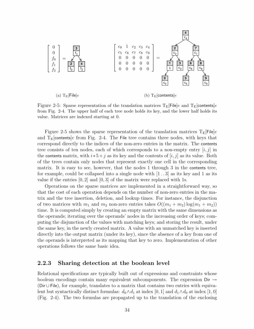
Figure 2-5: Sparse representation of the translation matrices TE[File]e and TE[contents]efrom Fig. 2-4. The upper half of each tree node holds its key, and the lower half holds itsvalue. Matrices are indexed starting at 0.

Figure 2-5 shows the sparse representation of the translation matrices TE[File]eand TE[contents]e from Fig. 2-4. The File tree contains three nodes, with keys thatcorrespond directly to the indices of the non-zero entries in the matrix. The contents

tree consists of ten nodes, each of which corresponds to a non-empty entry [i, j] inthe contents matrix, with i∗5+j as its key and the contents of [i, j] as its value. Bothof the trees contain only nodes that represent exactly one cell in the correspondingmatrix. It is easy to see, however, that the nodes 1 through 3 in the contents tree,for example, could be collapsed into a single node with [1 . . 3] as its key and 1 as itsvalue if the entries [0, 2] and [0, 3] of the matrix were replaced with 1s.

Operations on the sparse matrices are implemented in a straightforward way, sothat the cost of each operation depends on the number of non-zero entries in the ma-trix and the tree insertion, deletion, and lookup times. For instance, the disjunctionof two matrices with m1 and m2 non-zero entries takes O((m1 + m2) log(m1 + m2))time. It is computed simply by creating an empty matrix with the same dimensions asthe operands; iterating over the operands’ nodes in the increasing order of keys; com-puting the disjunction of the values with matching keys; and storing the result, underthe same key, in the newly created matrix. A value with an unmatched key is inserteddirectly into the output matrix (under its key), since the absence of a key from one ofthe operands is interpreted as its mapping that key to zero. Implementation of otheroperations follows the same basic idea.

2.2.3 Sharing detection at the boolean level

Relational specifications are typically built out of expressions and constraints whoseboolean encodings contain many equivalent subcomponents. The expression Dir →(Dir∪ File), for example, translates to a matrix that contains two entries with equiva-lent but syntactically distinct formulas: d0∧d1 at index [0, 1] and d1∧d0 at index [1, 0](Fig. 2-4). The two formulas are propagated up to the translation of the enclosing

34

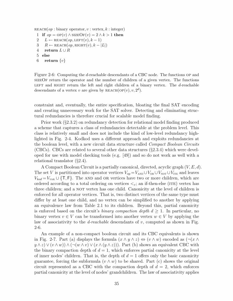
reach(op : binary operator, v : vertex, k : integer)1 if op = op(v) ∧ sizeOf(v) = 2 ∧ k > 1 then2 L← reach(op, left(v), k − 1)3 R← reach(op,right(v), k − |L|)4 return L ∪R5 else6 return {v}

Figure 2-6: Computing the d-reachable descendants of a CBC node. The functions op andsizeOf return the operator and the number of children of a given vertex. The functionsleft and right return the left and right children of a binary vertex. The d-reachabledescendants of a vertex v are given by reach(op(v), v, 2d).

constraint and, eventually, the entire specification, bloating the final SAT encodingand creating unnecessary work for the SAT solver. Detecting and eliminating struc-tural redundancies is therefore crucial for scalable model finding.

Prior work (§2.3.2) on redundancy detection for relational model finding produceda scheme that captures a class of redundancies detectable at the problem level. Thisclass is relatively small and does not include the kind of low-level redundancy high-lighted in Fig. 2-4. Kodkod uses a different approach and exploits redundancies atthe boolean level, with a new circuit data structure called Compact Boolean Circuits(CBCs). CBCs are related to several other data structures (§2.3.4) which were devel-oped for use with model checking tools (e.g. [49]) and so do not work as well with arelational translator (§2.4).

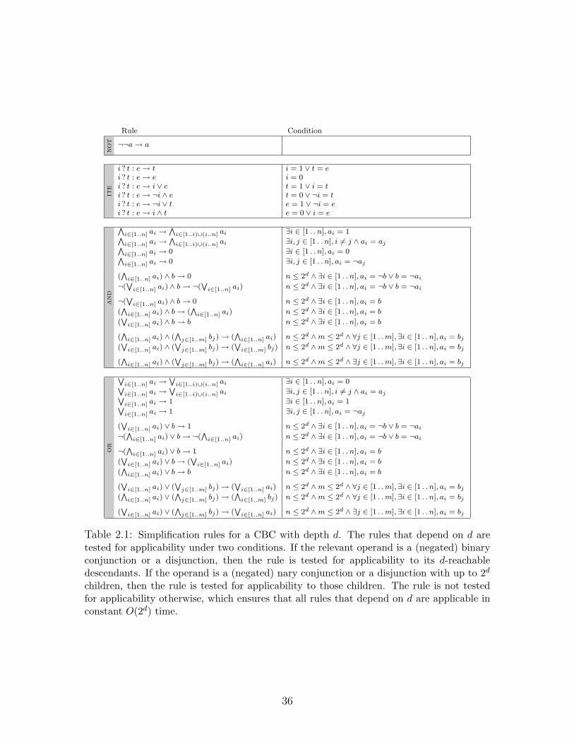
A Compact Boolean Circuit is a partially canonical, directed, acyclic graph (V, E, d).The set V is partitioned into operator vertices Vop =Vand∪Vor∪Vnot∪Vite and leavesVleaf =Vvar ∪ {T, F}. The and and or vertices have two or more children, which areordered according to a total ordering on vertices <v; an if-then-else (ite) vertex hasthree children; and a not vertex has one child. Canonicity at the level of children isenforced for all operator vertices. That is, two distinct vertices of the same type mustdiffer by at least one child, and no vertex can be simplified to another by applyingan equivalence law from Table 2.1 to its children. Beyond this, partial canonicityis enforced based on the circuit’s binary compaction depth d ≥ 1. In particular, nobinary vertex v ∈ V can be transformed into another vertex w ∈ V by applying thelaw of associativity to the d-reachable descendants of v, computed as shown in Fig.2-6.

An example of a non-compact boolean circuit and its CBC equivalents is shownin Fig. 2-7. Part (a) displays the formula (x ∧ y ∧ z) ⇔ (v ∧ w) encoded as (¬(x ∧y ∧ z)∨ (v ∧w))∧ (¬(w ∧ v)∨ (x∧ (y ∧ z))). Part (b) shows an equivalent CBC withthe binary compaction depth of d = 1, which enforces partial canonicity at the levelof inner nodes’ children. That is, the depth of d = 1 offers only the basic canonicityguarantee, forcing the subformula (v ∧ w) to be shared. Part (c) shows the originalcircuit represented as a CBC with the compaction depth of d = 2, which enforcespartial canonicity at the level of nodes’ grandchildren. The law of associativity applies

35

Rule Condition

not ¬¬a→ a

ite

i ? t : e→ t i = 1 ∨ t = ei ? t : e→ e i = 0i ? t : e→ i ∨ e t = 1 ∨ i = ti ? t : e→ ¬i ∧ e t = 0 ∨ ¬i = ti ? t : e→ ¬i ∨ t e = 1 ∨ ¬i = ei ? t : e→ i ∧ t e = 0 ∨ i = e

and

Vi∈[1..n] ai →

Vi∈[1..i)∪(i..n] ai ∃i ∈ [1 . . n], ai = 1V

i∈[1..n] ai →V

i∈[1..i)∪(i..n] ai ∃i, j ∈ [1 . . n], i 6= j ∧ ai = ajVi∈[1..n] ai → 0 ∃i ∈ [1 . . n], ai = 0Vi∈[1..n] ai → 0 ∃i, j ∈ [1 . . n], ai = ¬aj

(V

i∈[1..n] ai) ∧ b→ 0 n ≤ 2d ∧ ∃i ∈ [1 . . n], ai = ¬b ∨ b = ¬ai

¬(W

i∈[1..n] ai) ∧ b→ ¬(W

i∈[1..n] ai) n ≤ 2d ∧ ∃i ∈ [1 . . n], ai = ¬b ∨ b = ¬ai

¬(W

i∈[1..n] ai) ∧ b→ 0 n ≤ 2d ∧ ∃i ∈ [1 . . n], ai = b

(V

i∈[1..n] ai) ∧ b→ (V

i∈[1..n] ai) n ≤ 2d ∧ ∃i ∈ [1 . . n], ai = b

(W

i∈[1..n] ai) ∧ b→ b n ≤ 2d ∧ ∃i ∈ [1 . . n], ai = b

(V

i∈[1..n] ai) ∧ (V

j∈[1..m] bj)→ (V

i∈[1..n] ai) n ≤ 2d ∧m ≤ 2d ∧ ∀j ∈ [1 . . m], ∃i ∈ [1 . . n], ai = bj

(W

i∈[1..n] ai) ∧ (W

j∈[1..m] bj)→ (W

i∈[1..m] bj) n ≤ 2d ∧m ≤ 2d ∧ ∀j ∈ [1 . . m], ∃i ∈ [1 . . n], ai = bj

(V

i∈[1..n] ai) ∧ (W

j∈[1..m] bj)→ (V

i∈[1..n] ai) n ≤ 2d ∧m ≤ 2d ∧ ∃j ∈ [1 . . m], ∃i ∈ [1 . . n], ai = bj

or

Wi∈[1..n] ai →

Wi∈[1..i)∪(i..n] ai ∃i ∈ [1 . . n], ai = 0W

i∈[1..n] ai →W

i∈[1..i)∪(i..n] ai ∃i, j ∈ [1 . . n], i 6= j ∧ ai = ajWi∈[1..n] ai → 1 ∃i ∈ [1 . . n], ai = 1Wi∈[1..n] ai → 1 ∃i, j ∈ [1 . . n], ai = ¬aj

(W

i∈[1..n] ai) ∨ b→ 1 n ≤ 2d ∧ ∃i ∈ [1 . . n], ai = ¬b ∨ b = ¬ai

¬(V

i∈[1..n] ai) ∨ b→ ¬(V

i∈[1..n] ai) n ≤ 2d ∧ ∃i ∈ [1 . . n], ai = ¬b ∨ b = ¬ai

¬(V

i∈[1..n] ai) ∨ b→ 1 n ≤ 2d ∧ ∃i ∈ [1 . . n], ai = b

(W

i∈[1..n] ai) ∨ b→ (W

i∈[1..n] ai) n ≤ 2d ∧ ∃i ∈ [1 . . n], ai = b

(V

i∈[1..n] ai) ∨ b→ b n ≤ 2d ∧ ∃i ∈ [1 . . n], ai = b

(W

i∈[1..n] ai) ∨ (W

j∈[1..m] bj)→ (W

i∈[1..n] ai) n ≤ 2d ∧m ≤ 2d ∧ ∀j ∈ [1 . . m], ∃i ∈ [1 . . n], ai = bj

(V

i∈[1..n] ai) ∨ (V

j∈[1..m] bj)→ (V

i∈[1..m] bj) n ≤ 2d ∧m ≤ 2d ∧ ∀j ∈ [1 . . m], ∃i ∈ [1 . . n], ai = bj

(W

i∈[1..n] ai) ∨ (V

j∈[1..m] bj)→ (W

i∈[1..n] ai) n ≤ 2d ∧m ≤ 2d ∧ ∃j ∈ [1 . . m], ∃i ∈ [1 . . n], ai = bj

Table 2.1: Simplification rules for a CBC with depth d. The rules that depend on d aretested for applicability under two conditions. If the relevant operand is a (negated) binaryconjunction or a disjunction, then the rule is tested for applicability to its d-reachabledescendants. If the operand is a (negated) nary conjunction or a disjunction with up to 2d

children, then the rule is tested for applicability to those children. The rule is not testedfor applicability otherwise, which ensures that all rules that depend on d are applicable inconstant O(2d) time.

36

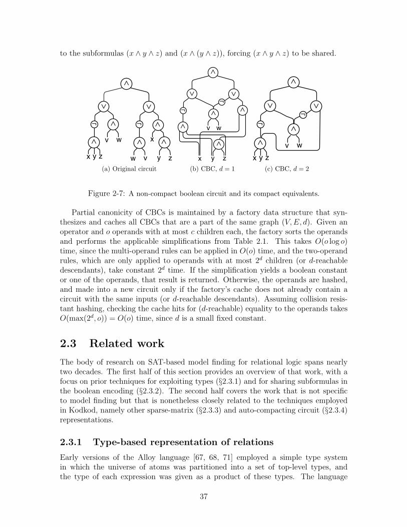
to the subformulas (x ∧ y ∧ z) and (x ∧ (y ∧ z)), forcing (x ∧ y ∧ z) to be shared.

∨

z

∧

x y

∧

v w

∧

w v

∧ x

∧

∧

zy

∨

¬ ¬

(a) Original circuit

∨ ∨

∧

∧

y zx

∧

¬

∧

¬

v w

∧

(b) CBC, d = 1

∨ ∨

∧

¬¬

v w

∧

z

∧

x y(c) CBC, d = 2

Figure 2-7: A non-compact boolean circuit and its compact equivalents.

Partial canonicity of CBCs is maintained by a factory data structure that syn-thesizes and caches all CBCs that are a part of the same graph (V, E, d). Given anoperator and o operands with at most c children each, the factory sorts the operandsand performs the applicable simplifications from Table 2.1. This takes O(o log o)time, since the multi-operand rules can be applied in O(o) time, and the two-operandrules, which are only applied to operands with at most 2d children (or d-reachabledescendants), take constant 2d time. If the simplification yields a boolean constantor one of the operands, that result is returned. Otherwise, the operands are hashed,and made into a new circuit only if the factory’s cache does not already contain acircuit with the same inputs (or d-reachable descendants). Assuming collision resis-tant hashing, checking the cache hits for (d-reachable) equality to the operands takesO(max(2d, o)) = O(o) time, since d is a small fixed constant.

2.3 Related work

The body of research on SAT-based model finding for relational logic spans nearlytwo decades. The first half of this section provides an overview of that work, with afocus on prior techniques for exploiting types (§2.3.1) and for sharing subformulas inthe boolean encoding (§2.3.2). The second half covers the work that is not specificto model finding but that is nonetheless closely related to the techniques employedin Kodkod, namely other sparse-matrix (§2.3.3) and auto-compacting circuit (§2.3.4)representations.

2.3.1 Type-based representation of relations

Early versions of the Alloy language [67, 68, 71] employed a simple type systemin which the universe of atoms was partitioned into a set of top-level types, andthe type of each expression was given as a product of these types. The language

37

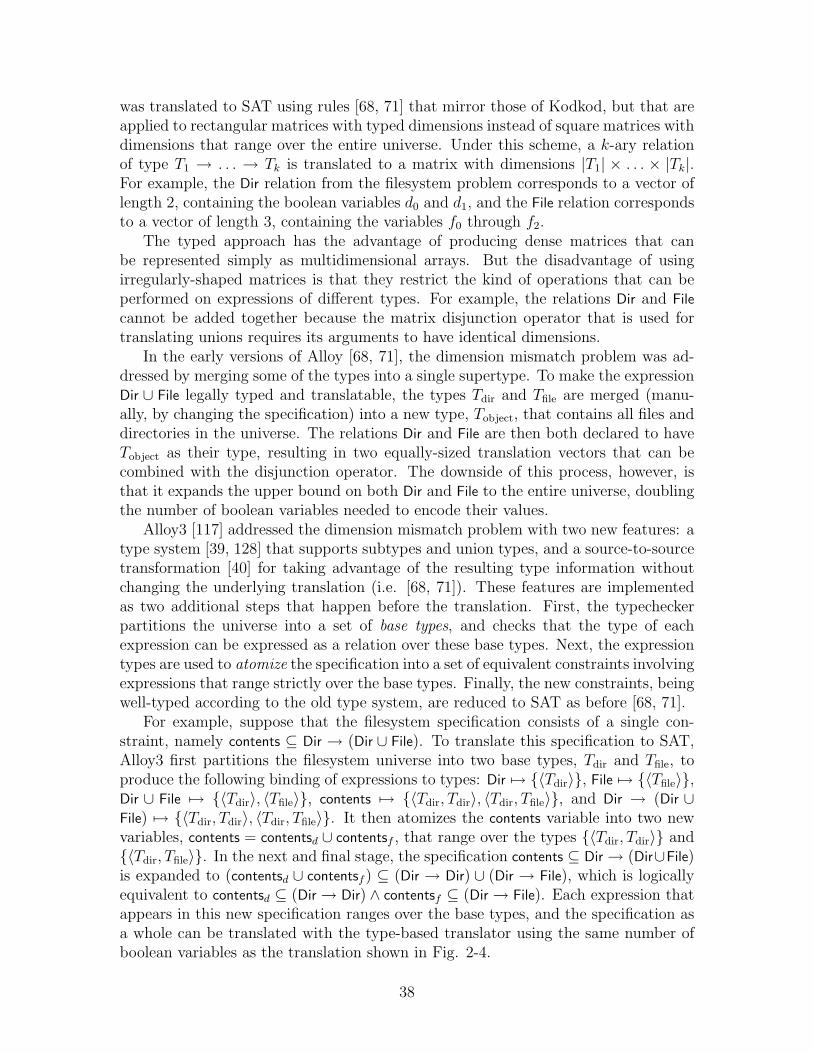
was translated to SAT using rules [68, 71] that mirror those of Kodkod, but that areapplied to rectangular matrices with typed dimensions instead of square matrices withdimensions that range over the entire universe. Under this scheme, a k-ary relationof type T1 → . . . → Tk is translated to a matrix with dimensions |T1| × . . . × |Tk|.For example, the Dir relation from the filesystem problem corresponds to a vector oflength 2, containing the boolean variables d0 and d1, and the File relation correspondsto a vector of length 3, containing the variables f0 through f2.

The typed approach has the advantage of producing dense matrices that canbe represented simply as multidimensional arrays. But the disadvantage of usingirregularly-shaped matrices is that they restrict the kind of operations that can beperformed on expressions of different types. For example, the relations Dir and File

cannot be added together because the matrix disjunction operator that is used fortranslating unions requires its arguments to have identical dimensions.

In the early versions of Alloy [68, 71], the dimension mismatch problem was ad-dressed by merging some of the types into a single supertype. To make the expressionDir ∪ File legally typed and translatable, the types Tdir and Tfile are merged (manu-ally, by changing the specification) into a new type, Tobject, that contains all files anddirectories in the universe. The relations Dir and File are then both declared to haveTobject as their type, resulting in two equally-sized translation vectors that can becombined with the disjunction operator. The downside of this process, however, isthat it expands the upper bound on both Dir and File to the entire universe, doublingthe number of boolean variables needed to encode their values.

Alloy3 [117] addressed the dimension mismatch problem with two new features: atype system [39, 128] that supports subtypes and union types, and a source-to-sourcetransformation [40] for taking advantage of the resulting type information withoutchanging the underlying translation (i.e. [68, 71]). These features are implementedas two additional steps that happen before the translation. First, the typecheckerpartitions the universe into a set of base types, and checks that the type of eachexpression can be expressed as a relation over these base types. Next, the expressiontypes are used to atomize the specification into a set of equivalent constraints involvingexpressions that range strictly over the base types. Finally, the new constraints, beingwell-typed according to the old type system, are reduced to SAT as before [68, 71].

For example, suppose that the filesystem specification consists of a single con-straint, namely contents ⊆ Dir → (Dir ∪ File). To translate this specification to SAT,Alloy3 first partitions the filesystem universe into two base types, Tdir and Tfile, toproduce the following binding of expressions to types: Dir 7→ {〈Tdir〉}, File 7→ {〈Tfile〉},Dir ∪ File 7→ {〈Tdir〉, 〈Tfile〉}, contents 7→ {〈Tdir, Tdir〉, 〈Tdir, Tfile〉}, and Dir → (Dir ∪File) 7→ {〈Tdir, Tdir〉, 〈Tdir, Tfile〉}. It then atomizes the contents variable into two newvariables, contents = contentsd ∪ contentsf , that range over the types {〈Tdir, Tdir〉} and{〈Tdir, Tfile〉}. In the next and final stage, the specification contents ⊆ Dir→ (Dir∪File)is expanded to (contentsd ∪ contentsf ) ⊆ (Dir → Dir) ∪ (Dir → File), which is logicallyequivalent to contentsd ⊆ (Dir→ Dir) ∧ contentsf ⊆ (Dir→ File). Each expression thatappears in this new specification ranges over the base types, and the specification asa whole can be translated with the type-based translator using the same number ofboolean variables as the translation shown in Fig. 2-4.

38

The atomization approach, however, does not work well for specifications withtransitive closure. Because there is no efficient way to atomize transitive closureexpressions [40] such as contents in the toy filesystem, Alloy3 handles problems withclosure by merging the domain and range types of each closure expression into a singlebase type. In the case of the filesystem problem, this leads to the merging of file anddirectory types into a single type and, consequently, to the doubling in the numberof boolean variables needed to represent each relation.

2.3.2 Sharing detection at the problem level

Formal specifications of software systems often make use of quantified formulas whoseground form contains many identical subcomponents. For example, the specificationof a filesystem that disallows sharing of contents among directories (e.g. via hardlinks) may include the constraint ∀ p, d: Dir | ¬p=d ⇒ no (p.contents ∩ d.contents),which grounds out to

(¬{〈d0〉}={〈d0〉}⇒ no ({〈d0〉}.contents ∩ {〈d0〉}.contents)) ∧(¬{〈d0〉}={〈d1〉}⇒ no ({〈d0〉}.contents ∩ {〈d1〉}.contents)) ∧(¬{〈d1〉}={〈d0〉}⇒ no ({〈d1〉}.contents ∩ {〈d0〉}.contents)) ∧(¬{〈d1〉}={〈d1〉}⇒ no ({〈d1〉}.contents ∩ {〈d1〉}.contents))

in a two-directory universe. Alloy3’s sharing detection mechanism [117, 119] focuseson ensuring that all occurrences of a given ground component, such as {〈d0〉}.contents,share the same boolean encoding in memory.

The scheme works in two stages: a detection phase, in which the AST of a spec-ification is traversed and each node is annotated with a syntactic template, and atranslation phase, in which the template annotations are used to ensure sharing. Forthe above example, the first phase produces a set of template annotations that in-cludes ¬p=d 7→ “¬? = ?”, p.contents 7→ “?.contents”, and d.contents 7→ “?.contents”.1

In the next phase, the translator keeps a cache for each template, which stores thetranslations of all ground forms that instantiate the template. A ground form fora node is then translated only if its translation is missing from the cache of thenode’s template. For example, when visiting d.contents in the environment {p7→{〈d0〉},d7→{〈d0〉}}, the translator will find that the cache of “?.contents” contains a translationfor {〈d0〉}.contents, because p.contents, which is translated first, has the same groundform in the given environment. The end result is that each occurrence of the groundexpression {〈d0〉}.contents (and, similarly, {〈d1〉}.contents) translates to the same ma-trix in memory.

Unlike the template approach, Kodkod’s CBC approach ensures not only that thetranslations for syntactically equivalent ground expressions are shared, but also that¬{〈d0〉}= {〈d1〉} and ¬{〈d1〉}={〈d0〉} are translated to the same circuit. The templatescheme misses the latter opportunity for sharing because the two instantiations of thetemplate ¬?=? are syntactically distinct. In general, the set of redundancies detected

1Alloy3 creates a unique ID for each template rather than a syntactic representation such as“?.contents”; the syntactic representation is used in the text for presentational clarity.

39

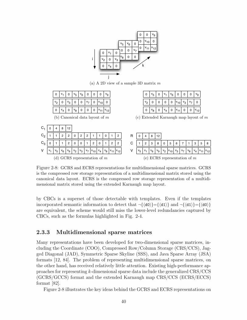
00 v9v100 0

v110 v12v6v5 0

00 v7

0v8 0v10 0

0v2 v3v40 0

i

j

k

(a) A 2D view of a sample 3D matrix m

00 v9v6v5 0v10 0

v100 000 v70v2 v3

v110 v120v8 0v40 0

(b) Canonical data layout of m

00 v9v6v5 0v10 0

v100 000 v70v2 v3

v110 v120v8 0v40 0

(c) Extended Karnaugh map layout of m

1240 8

21012 102 211 2

v12v11v8v10v7 v4v2v9 v3v5v1 v6

22121 002 010 1

C1C2

V

C3

(d) GCRS representation of m

v12v11v4v7v3 v8v2v9 v10v1v5 v6V

85376 108 521 3C

1240 8R

(e) ECRS representation of m

Figure 2-8: GCRS and ECRS representations for multidimensional sparse matrices. GCRSis the compressed row storage representation of a multidimensional matrix stored using thecanonical data layout. ECRS is the compressed row storage representation of a multidi-mensional matrix stored using the extended Karnaugh map layout.

by CBCs is a superset of those detectable with templates. Even if the templatesincorporated semantic information to detect that ¬{〈d0〉}={〈d1〉} and ¬{〈d1〉}={〈d0〉}are equivalent, the scheme would still miss the lower-level redundancies captured byCBCs, such as the formulas highlighted in Fig. 2-4.

2.3.3 Multidimensional sparse matrices

Many representations have been developed for two-dimensional sparse matrices, in-cluding the Coordinate (COO), Compressed Row/Column Storage (CRS/CCS), Jag-ged Diagonal (JAD), Symmetric Sparse Skyline (SSS), and Java Sparse Array (JSA)formats [12, 84]. The problem of representing multidimensional sparse matrices, onthe other hand, has received relatively little attention. Existing high-performance ap-proaches for representing k-dimensional sparse data include the generalized CRS/CCS(GCRS/GCCS) format and the extended Karnaugh map CRS/CCS (ECRS/ECCS)format [82].

Figure 2-8 illustrates the key ideas behind the GCRS and ECRS representations on

40

a sample three dimensional matrix. The GCRS format is based on the canonical datalayout for multidimensional arrays [24], in which an nk matrix is represented usingn one-dimensional arrays of size nk−1, with the matrix index [i1, . . . , ik] mapping tothe index

∑kj=2 ijn

j−2 of the ith1 array (Fig. 2-8b). The ECRS format is based onthe extended Karnaugh map layout [83] which represents multidimensional arrayswith collections of two-dimensional matrices. An n × n × n matrix, for example, isrepresented with n matrices of size n × n, where the 3-dimensional index [i1, i2, i3]maps to the index [i1, i3] of the ith2 matrix. The three matrices are laid out in memorywith n arrays of length n2, with the index [i1, i2, i3] mapping to the index i2n + i3 ofthe ith1 array (Fig. 2-8c).

Once a multidimensional sparse matrix is laid out in memory, it can be compressedusing a variation on the standard CRS format for 2-dimensional arrays. Given annk matrix m, GCRS encodes its canonical data representation CDL(m) with arraysC1, . . . , Ck and V (Fig. 2-8d). The V array stores the non-zero values of thematrix, obtained by scanning the rows of CDL(m) from left to right. The C1 arraystores the locations in V that start a row. In particular, if V [l] = m[i1, . . . , ik] thenC1[i1] ≤ l < C1[i1 + i]. By convention, C1 has n+1 elements with C1[n] = |V |, where|V | is the length of V . Arrays C2, . . . , Ck store the non-row indices of the elementsin V ; i.e., if V [l] = m[i1, i2, . . . , ik], then C2[l] = i2, . . . , Ck[l] = ik. ECRS (for three-dimensional matrices) encodes EKM(m), the extended Karnaugh map representationof m, with three arrays: R, C, and V (Fig. 2-8e). The R and V arrays are definedin the same way as the C1 and V arrays produced by GCRS. The C array stores thecolumn indices of the non-zero elements in EKM(m); that is, V [l] = m[i1, i2, i3] thenC[l] = i2n + i3.

Compared to Kodkod’s sparse matrices, GCRS and ECRS provide better averageaccess time for a given index.2 For an nk matrix with an average of d non-zeroesper row, the value at a given index can be retrieved in O(log d) time for both GCRSand ECRS; the Kodkod representation requires O(log nd) time. The Kodkod rep-resentation, however, has several features that make it more suitable for use witha relational translator than GCRS or ECRS. First, Kodkod matrices are mutable,which is crucial for the translation of expressions (e.g. set comprehensions) whosematrices must be filled incrementally. Neither GCRS nor ECRS support mutation.Second, the representation of a Kodkod matrix shrinks as the number of consecutive1s in its cells increases, which is important for efficient translation of problems thathave large partial models or that use built-in constants such as the universal relation.GCRS and ECRS, for example, need O(nk) space to represent the universal relationof arity k over an n-atom universe; Kodkod needs just one node. Finally, disjunction,multiplication and other operations are straightforward to implement for Kodkodmatrices. Corresponding operations on GCRS and ECRS matrices, in contrast, aremuch trickier to design: the published addition and multiplication algorithms forthese matrices work only when one of the operands is represented sparsely and theother fully [82].

2Worst case access time for all three encodings is logarithmic in the number of non-zero elements.

41

2.3.4 Auto-compacting circuits

The choice of circuit representation in a model checker affects the efficiency of theoverall tool in two ways [18]. First, a compact representation saves memory, en-abling faster processing of larger problems. Second, it eliminates redundancies inthe boolean encoding, which is particularly important for SAT-based tools. Theseconcerns have been addressed in the literature with three different circuit representa-tions, designed to work with different model checking backends: Boolean ExpressionDiagrams (BEDs) [6], which are designed for use with BDD-based model checkers[95]; Reduced Boolean Circuits (RBCs) [1]; and And-Inverter Graphs (AIGs) [19, 78],which are used in SAT-based tools for bounded model checking [49, 73].

BEDs, RBCs and AIGs are similar to CBCs in that they define a graph over oper-ator and leaf vertices which satisfies a set of partial canonicity invariants. Of the four,BEDs support the largest number of operators (with every 2-input boolean functionrepresented by its own BED vertex), and AIGs support the fewest operators (allowingonly conjunctions and negations). RBCs support three operators: conjunction, nega-tion, and equivalence. CBCs are the only representation that supports multi-inputand and or gates, which is crucial for efficient translation of quantified formulas.In particular, a quantified formula such as ∀x1, . . . , xk : X | F (x1, . . . , xk) is trans-lated as a conjunction of |X|k circuits that encode the ground forms of F (x1, . . . , xk).CBCs represent this conjunction using a single gate with |X|k inputs. The other threerepresentations use |X|k − 1 binary gates.

In addition to supporting multi-input gates, CBCs also use different simplificationrules than BEDs, AIGs, and RBCs. Both BEDs and AIGs employ two-level rewriterules (i.e. rules that take into account operands’ children), which have been shown toinhibit rather than promote subformula sharing [18]. Figure 2-9 displays an exampleof such a rule, and how it interferes with sharing. A recent implementation of AIGs[19] limited its use of two-level rules to those that do not interfere with sharing. Theseare a superset of the rules employed by CBCs (Table 2.1). RBCs do not performany two-level simplifications. Rather, the two-level redundancies missed during theconstruction of RBCs can be caught with an optional post-construction step [18],which reduces the number of gates in an RBC by up to 10%.

Of the four circuit representations, RBCs are fastest to construct, since theirsimplification rules take constant time to apply. The construction of a given CBCis also constant, if only binary gates are used. The use of n-ary gates slows theconstruction of a specific circuit down to O(max(i log i, c)) time, where i is the numberof inputs to the circuit and c is the number of those inputs’ children. This, however,is not a bottleneck in practice (§2.4). The complexity of BED and AIG constructionis not known [18], because the two-level rules used by BED and AIGs can trigger anunknown number of recursive calls to the circuit creation procedure. The only CBCrules that may trigger a recursive call are the last four ite rules in Table 2.1, butthe resulting recursion bottoms out immediately since the only rules applicable in therecursive call are the and and or rules, which are implemented without calling thefactory.3

3Note that each and and or rule, when applicable, simply eliminates some or all of the inputs.

42

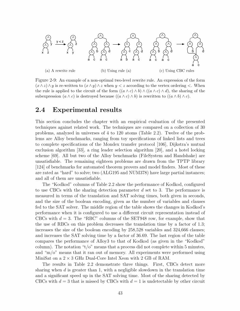
y < zy

∧

∧

x z

z

∧

∧

x y

(a) A rewrite rule

b

∧

∧

a c

d

∧

∧

a c

∧

c

∧

∧

a b

d

∧

∧

a c

∧

(b) Using rule (a)

b

∧

∧

a c

d

∧

∧

a c

∧

b

∧

∧

a c

d

∧

∧

(c) Using CBC rules

Figure 2-9: An example of a non-optimal two-level rewrite rule. An expression of the form(x∧ z)∧ y is re-written to (x∧ y)∧ z when y < z according to the vertex ordering <. Whenthe rule is applied to the circuit of the form ((a ∧ c) ∧ b) ∧ ((a ∧ c) ∧ d), the sharing of thesubexpression (a ∧ c) is destroyed because ((a ∧ c) ∧ b) is rewritten to ((a ∧ b) ∧ c).

2.4 Experimental results

This section concludes the chapter with an empirical evaluation of the presentedtechniques against related work. The techniques are compared on a collection of 30problems, analyzed in universes of 4 to 120 atoms (Table 2.2). Twelve of the prob-lems are Alloy benchmarks, ranging from toy specifications of linked lists and treesto complete specifications of the Mondex transfer protocol [106], Dijkstra’s mutualexclusion algorithm [33], a ring leader selection algorithm [20], and a hotel lockingscheme [69]. All but two of the Alloy benchmarks (FileSystem and Handshake) areunsatisfiable. The remaining eighteen problems are drawn from the TPTP library[124] of benchmarks for automated theorem provers and model finders. Most of theseare rated as “hard” to solve; two (ALG195 and NUM378) have large partial instances;and all of them are unsatisfiable.

The “Kodkod” columns of Table 2.2 show the performance of Kodkod, configuredto use CBCs with the sharing detection parameter d set to 3. The performance ismeasured in terms of the translation and SAT solving times, both given in seconds,and the size of the boolean encoding, given as the number of variables and clausesfed to the SAT solver. The middle region of the table shows the changes in Kodkod’sperformance when it is configured to use a different circuit representation instead ofCBCs with d = 3. The “RBC” columns of the SET948 row, for example, show thatthe use of RBCs on this problem decreases the translation time by a factor of 1.3;increases the size of the boolean encoding by 258,528 variables and 324,666 clauses;and increases the SAT solving time by a factor of 36.69. The last region of the tablecompares the performance of Alloy3 to that of Kodkod (as given in the “Kodkod”column). The notation “t/o” means that a process did not complete within 5 minutes,and “m/o” means that it ran out of memory. All experiments were performed usingMiniSat on a 2× 3 GHz Dual-Core Intel Xeon with 2 GB of RAM.

The results in Table 2.2 demonstrate three things. First, CBCs detect moresharing when d is greater than 1, with a negligible slowdown in the translation timeand a significant speed up in the SAT solving time. Most of the sharing detected byCBCs with d = 3 that is missed by CBCs with d = 1 is undetectable by other circuit

43

Ko

dk

od

& C

BC

s w

ith

d=

3K

od

ko

d &

CB

Cs w

ith

d=

1K

od

ko

d &

RB

Cs

Allo

y3

pro

ble

muniv

.tr

ansl.(s

)so

lve(s

)variab

les

cla

uses

transl

so

lve

variab

les cla

uses

transl

so

lve

variab

les

cla

uses

transl.

so

lve

variab

les

cla

uses

AW

D.A

241

51

0.4

7109.6

438459

91389

!1.1

2!

1+

0+

0!

1.1

7!

1.2

5+

19362

+2855

7!

29

.97

!0.6

3+

124

67

+3

25

35

5

AW

D.O

pT

ota

l51

0.2

50.0

00

0!

10 s

ec

+0

+0

!1.1

20 s

ec

+0

+0

!54

.56

2.3

3 s

ec

+4

32

56

+3

81

45

8

AW

D.Ig

no

re51

0.3

915.0

130821

62457

!0.9

3!

1+

0+

0!

1.0

2!

0.7

7+

14285

+1764

4!

30

.46

!0.2

8+

125

92

+3

24

35

5

AW

D.T

ransfe

r41

0.3

686.5

121605

48809

!0.9

2!

1+

0+

0!

0.9

7!

0.9

8+

10146

+1383

7!

41.9

!1.2

1+

69

51

+1

40

32

5

Dijkstr

a60

41.0

317.9

1310718

1770316

!0.9

9!

1+

0+

0!

0.9

3!

1.7

4+

400448

-46228

4m

/om

/om

/om

/o

FileS

yste

m90

13.3

12.1

9256025

702536

!0.9

8!

0.7

2+

150

+420

!1.0

9!

0.1

5+

215224

+32945

8!

12

.77

!6.6

1+

20

03

25

+1

693

33

4

Hand

shake

10

0.2

30.5

04913

11313

!0.9

6!

0.9

9+

0+

0!

1.0

7!

2.2

5+

77

24

+2025

7!

6.5

5!

0.8

9+

34

99

+27

17

2

Lis

t.E

mp

ties

120

65.8

812.1

12547227

7165003

!0.9

7!

0.2

9+

360

+300

!1.3

2!

2.4

8+

2342214

+3

38096

6m

/om

/om

/om

/o

Lis

t.R

eflexiv

e28

0.5

810.1

434925

92537

!1.0

3!

1.1

4+

56

+42

!1.1

8!

1.7

+24020

+3552

3!

23

.52

t/o

+1

95

01

+2

38

79

1

Lis

t.S

ym

m16

0.2

319.1

77285

18199

!1.0

3!

0.8

2+

24

+16

!0.9

4!

1.1

2+

39

62

+580

8!

13

.88

!0

.5+

58

56

+51

67

5

Rin

gE

lectio

n16

0.6

622.8

530303

98305

!0.9

8!

0.8

9+

24

+24

!1.0

4!

0.6

4+

20709

+1878

9!

15

.27

!2.1

7+

127

55

+2

08

21

1

Tre

es

79.5

354.8

4407399

349797

!0.6

9!

1.4

5+

27083

+82719

!0.6

6!

2.4

8+

331355

+21227

8m

/om

/om

/om

/o

ALG

195

14

0.4

60.0

432184

96606

!0.9

8!

0.6

7+

8+

196

!1

.2!

0.7

1+

20178

+3371

0!

101

.87

!48

.79

+16

32

24

+7

37

90

2

ALG

197

14

0.4

20.0

228556

83370

!1.0

4!

0.6

3+

43

+547

!1.1

7!

1.4

6+

18259

+3002

6!

25

.93

!27

.63

+2

14

68

+1

12

41

1

ALG

212

76.9

547.3

11072205

1032354

!0.9

8!

1+

0+

0!

1.4

!2.0

8+

721464

+39569

1t/

ot/

ot/

ot/

o

CO

M008

12

0.5

95.4

69624

15827

!0.9

5!

1+

0+

0!

0.9

8!

2.3

5+

68

03

+812

3!

8.7

3!

0.4

5+

98

23

+84

74

0

GE

O091

20

8.8

257.5

0106350

206029

!1.0

2!

1.6

8+

32880

+48150

!1

.2t/

o+

112559

+15391

9!

1.0

8t/

o+

635

29

+6

83

95

9

GE

O092

16

2.7

95.1

148521

92844

!1.0

1!

1.1

7+

12818

+18586

!1.0

2!

1.4

6+

47626

+6419

4!

10

.56

!1.8

7+

344

44

+4

99

78

4

GE

O115

18

5.0

646.1

3109022

190839

!1.0

8!

0.8

6+

25818

+40242

!1.4

5t/

o+

99463

+13254

4t/

ot/

ot/

ot/

o

GE

O158

16

2.7

711.0

746673

89825

!1.0

2!

1.2

+12818

+18586

!0.9

5!

4.1

5+

46598

+6316

6!

10

.72

!33

.28

+3

40

40

+4

88

88

7

GE

O159

16

8.8

327.5

487241

200377

!1.0

1!

1.5

1+

16738

+25418

!0.9

6!

2.0

4+

74058

+10761

8t/

ot/

ot/

ot/

o

LA

T258

71.5

27.5

6205647

337033

!0.9

5!

1.2

2+

14

+0

!1.3

9!

1.5

1+

116703

+11730

5m

/om

/om

/om

/o

ME

D007

35

1.6

239.3

0130817

268666

!1

!1

+0

+0

!1.2

8!

1.6

6+

107203

+11654

8!

22

.32

!3.2

3+

59

68

+5

69

92

7

ME

D009

35

1.5

144.0

7130817

268667

!1.0

8!

1.0

1+

0+

0!

1.4

!1.6

1+

107203

+11654

8!

26

.75

!1.2

2+

59

69

+5

69

92

8

NU

M374

50.6

534.4

462112

198128

!1.1

6!

1.0

1+

0+

0!

1.2

4!

1.1

9+

33861

+6164

6!

13

.94

!1.0

2+

81

17

+93

44

5

NU

M378

22

0.4

20.0

00

0!

0.8

60 s

ec

+0

+0

!1.1

90 s

ec

+0

+0

m/o

m/o

m/o

m/o

SE

T943

70.4

111.2

516009

39950

!0.9

9!

1.2

+7

+28

!0.9

9!

2.1

6+

10493

+1448

8!

29

!11

.35

+91

15

+61

09

0

SE

T948

14

4.1

02.0

8339151

870110

!0.9

7!

23.5

2+

14

+56

!1

.3!

116.8

7+

258528

+32466

6!

35

.44

!19

.06

+14

32

43

+1

122

97

4

SE

T967

40.3

70.0

914659

45941

!0.9

8!

0.9

2+

16

+48

!1.0

2!

1.5

4+

64

16

+1142

5!

8.5

8!

4.2

4+

51

35

+29

06

3

TO

P020

10

18.0

348.9

32554124

4264114

!0.9

9!

1+

0+

0!

1.3

5!

1.1

8+

1417260

+1

52250

0m

/om

/om

/om

/o

ave

rag

e:

ave

rag

e:

!0.9

9!

1.7

!1.1

2!

5.6

3!

24

.94

!8.7

8

Alloy benchmarks TPTP benchmarks

Tab

le2.

2:E

valu

atio

nof

Kod

kod’

str

ansl

atio

nop

tim

izat

ions

.T

hefir

stre

gion

ofth

eta

ble

show

sth

eba

selin

epe

rfor

man

ceof

Kod

kod

(usi

ngC

BC

sof

dept

h3)

,w

ith

the

tran

slat

ion

and

solv

ing

tim

esgi

ven

inse

cond

s.T

hene

xttw

ore

gion

sco

mpa

reth

epe

rfor

man

ceof

Kod

kod

wit

hba

sic

CB

Cs

(d=

1)an

dw

ith

RB

Cs

toth

eba

selin

e.T

hela

stre

gion

com

pare

sA

lloy3

toth

eba

selin

e,w

here

m/o

mea

nsth

ata

proc

ess

ran

out

ofm

emor

yan

dt/

om

eans

that

itdi

dno

tco

mpl

ete

wit

hin

5m

inut

es.

44

representations, since they perform equivalence checking exclusively at the level ofchildren (i.e. at d = 1). Second, while the construction of CBCs takes slightly moretime than that of RBCs, a CBC-based translation is faster in practice because fewergates need to be constructed. The CBC circuits are also solved, on average, 5.63 timesfaster than the corresponding RBCs (not counting the two RBCs on which the SATsolver timed out). Third, the comparison between Alloy3 and Kodkod shows that atranslation based on boolean-level sharing detection and sparse matrices is roughly anorder of magnitude more effective than a translation that uses problem-level sharingdetection and typed matrices. Alloy3 either timed out or ran out of memory on 11out of 30 problems. It translated the remaining ones 24.94 times slower than Kodkod,producing significantly larger boolean formulas that, in turn, took 8.78 times longerto solve.

45

46

Chapter 3

Detecting Symmetries

Many problems exhibit symmetries. A symmetry is a permutation of atoms in aproblem’s universe that takes models of the problem to other models and non-modelsto other non-models. The toy filesystem (Fig. 2-2), for example, has six symmetries,each of which permutes the file atoms and maps the directory atoms to themselves.Figures 3-1 and 3-2 show the action of these symmetries on two sets of bindingsfrom filesystem variables to constants: all bindings in Fig. 3-1 satisfy the filesystemconstraints and all bindings in Fig. 3-2 violate them. Because symmetries partitiona problem’s state space into classes of equivalent bindings, a model, if one exists, canbe found by examining a single representative of each equivalence class. For problemswith large state spaces but few classes of equivalent bindings, exploiting, or breaking,symmetries can lead to exponential gains in model finding efficiency.

Model finders exploit symmetries in two ways. Dynamic techniques explore thestate space of a problem directly, with a dedicated algorithm that employs symmetry-based heuristics to guide the search [70, 93, 151, 152]. Static approaches use a black-box search engine, such as a SAT solver, on a problem that has been augmented withsymmetry breaking predicates [27, 55, 116]. These predicates consist of constraints thatare true of at least one binding in each equivalence class (but not all); adding them tothe translation of a problem blocks a backtracking solver from exploring regions of thesearch space that contain no representative bindings. Kodkod, like other SAT-basedmodel finders [117, 25], takes the static approach to symmetry breaking.

To use either approach, however, a model finder must first find a set of symmetriesto break. In the case of logics accepted by traditional model finders, symmetrydetection is straightforward. Given a universe of typed atoms, every permutationthat maps atoms of the same type to one another is a symmetry of any problemdefined over that universe [70]. Atoms of the same type can be freely interchangedbecause traditional logics provide no means of referring to individual atoms. Butlogics accepted by model extenders such as Kodkod and IDP1.3 do, which makesinterchangeable atoms, and therefore symmetries, hard to identify. This chapterpresents a new greedy technique for finding a useful subset of the available symmetriesin the context of model extension. The technique is shown to be correct, locallyoptimal, effective in practice, and more scalable than a complete symmetry discoverymethod based on graph automorphism detection.

47

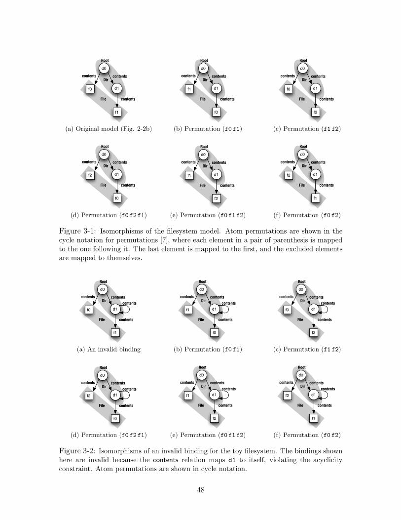
d0

d1f0

f1

contentscontents

contents

Root

Dir

File

(a) Original model (Fig. 2-2b)

d0

d1f1

f0

contentscontents

contents

Root

Dir

File

(b) Permutation (f0 f1)

d0

d1f0

f2

contentscontents

contents

Root

Dir

File

(c) Permutation (f1 f2)

d0

d1f2

f0

contentscontents

contents

Root

Dir

File

(d) Permutation (f0 f2 f1)

d0

d1f1

f2

contentscontents

contents

Root

Dir

File

(e) Permutation (f0 f1 f2)

d0

d1f2

f1

contentscontents

contents

Root

Dir

File

(f) Permutation (f0 f2)

Figure 3-1: Isomorphisms of the filesystem model. Atom permutations are shown in thecycle notation for permutations [7], where each element in a pair of parenthesis is mappedto the one following it. The last element is mapped to the first, and the excluded elementsare mapped to themselves.

d0

d1f0

f1

contentscontents

contents

Root

Dir

File

contents

(a) An invalid binding

d0

d1f1

f0

contentscontents

contents

Root

Dir

File

contents

(b) Permutation (f0 f1)

d0

d1f0

f2

contentscontents

contents

Root

Dir

File

contents

(c) Permutation (f1 f2)

d0

d1f2

f0

contentscontents

contents

Root

Dir

File

contents

(d) Permutation (f0 f2 f1)

d0

d1f1

f2

contentscontents

contents

Root

Dir

File

contents

(e) Permutation (f0 f1 f2)

d0

d1f2

f1

contentscontents

contents

Root

Dir

File

contents

(f) Permutation (f0 f2)

Figure 3-2: Isomorphisms of an invalid binding for the toy filesystem. The bindings shownhere are invalid because the contents relation maps d1 to itself, violating the acyclicityconstraint. Atom permutations are shown in cycle notation.

48

3.1 Symmetries in model extension

When configured or analyzed declaratively, systems with interchangeable componentsgive rise to model finding (or extension) problems with sets of symmetric atoms.These symmetries, in turn, induce equivalences or isomorphisms among bindings inthe problem’s state space. More precisely, a symmetry is a permutation of atoms ina problem’s universe that acts on a model of the problem to produce a model and ona non-model to produce a non-model. The action of a symmetry on a binding fromvariables to relational constants is defined as follows: a symmetry acts on a bindingby acting on each of its constants; on a constant by acting on each of its tuples;and on a tuple by acting on each of its atoms. Two bindings that are related by asymmetry are said to be isomorphic.

The set of symmetries of a problem P , denoted by Sym(P ), defines an equivalencerelation on the bindings that comprise the state space of P . Two bindings b and b′ areequivalent if b′ = l(b) for some l ∈ Sym(P ). Because equivalent bindings all satisfyor all violate P , it suffices to test one binding in each equivalence class inducedby Sym(P ) to find a model of P . Many practical problems, especially in boundedverification, have an exponentially large state space but only a polynomial numberof equivalence classes [117]. Exploitation of symmetries, or symmetry breaking, iscrucial for making such problems tractable [27, 111].

Until recently, much of the work on symmetries in model finding has focused onthe design of better symmetry breaking methods [70, 93, 151, 152, 116]. Symmetrydetection has received less attention because discovering symmetries of a traditionalmodel finding problem is straightforward. If a problem P is specified in an unsortedlogic, then Sym(P ) contains every permutation of atoms in the universe of P ; if thelogic is typed, then Sym(P ) consists of all permutations that map atoms of the sametype to one another [70]. These results, however, no longer hold when a standardlogic is extended to support partial models. If P is specified as a model extensionproblem that references individual atoms, as it may be in bounded relational logic,finding Sym(P ) becomes intractable.

Consider, for example, the toy filesystem from the previous chapter and twocandidate symmetries, l1 = (f0 f2) and l2 = (d0 d1).1 Both permutations respectthe intrinsic “types” in the filesystem universe, mapping directories to directoriesand files to files. When the two are applied to the model in Fig. 2-2b, however,only l1 yields a model (Fig. 3-1f). The permutation l2 yields the following bind-ing, which satisfies the filesystem specification but violates the bound constraintson the contents and Root relations: {File 7→ {〈f0〉, 〈f1〉}, Dir 7→ {〈d1〉, 〈d0〉}, Root 7→{〈d1〉}, contents 7→{〈d1,d0〉,〈d1,f0〉,〈d0,f1〉}}.

This example reveals two important properties of untyped model extension prob-lems.2 First, any permutation is a symmetry of a specification, by the result from

1The cycle notation for permutations is explained in Fig. 3-1.2All results from this chapter apply to other model extension logics, such as IDP, which restrict

the use of constants to type or partial model constraints (i.e. v = c, v ⊆ c, and c ⊆ v where v is avariable and c is a constant). If constants can be used freely, then Thm. 3.1 describes a subset ofSym(P ) rather than all of it; that is, only the ⇐ direction of the theorem holds.

49

traditional model finding (Lemma 3.1). The permutation l2, for example, is a sym-metry of the filesystem specification even though it is not a symmetry of the entireproblem. Second, a permutation is a symmetry of a set of bound constraints only if itmaps each constant within those bounds to itself (Lemma 3.2). The permutation l1 isa symmetry of the filesystem bounds and of the entire problem. As a result, Sym(P )for a Kodkod problem P is the set of all permutations that map each constant in P ’sbounds to itself (Thm. 3.1). This, however, means that finding Sym(P ) is as hardas graph automorphism detection (Thm. 3.2), which has no known polynomial timesolution [8].

Lemma 3.1 (Symmetries of specifications). If S is a bounded relational specificationover a (finite) universe U , then every permutation l : U → U is a symmetry of S.

Proof. Since S is a specification in a standard untyped logic (i.e. it contains noconstants), the symmetry result from traditional model finding applies [70].

Lemma 3.2 (Symmetries of bounds). Let U be a finite universe and let B be a set ofbounds of the form v :k [cL, cU ], where v is a variable of arity k and cL, cU ∈ 2Uk

. Apermutation l : U → U is a symmetry of B if and only if l(c) = c for each relationalconstant c that occurs in B.

Proof. (⇐, by contradiction). Suppose that l(c) = c for all c in B and that l is nota symmetry of B. Then, there must be some binding b from variables in B to sets oftuples that satisfies B, written as b |= B, but l(b) 6|= B. For this to be true, there mustalso be some v :k [cL, cU ] in B such that cL 6⊆ l(b(v)) or l(b(v)) 6⊆ cU . Since b |= B,cL ⊆ b(v) ⊆ cU . Let x be the difference between b(v) and cL, i.e. x = b(v) \ cL. Thisleads to l(b(v)) = l(cL ∪x) = l(cL)∪ l(x) = cL ∪ l(x), which implies that cL ⊆ l(b(v)).So it must be the case that l(b(v)) 6⊆ cU . But this cannot be true, because the factthat b(v) ⊆ cU and that l(cU) = cU together imply that l(b(v)) ⊆ l(cU) ⊆ cU .

(⇒, by contradiction). Suppose that B is a set of bounds and that l is a symmetryof B with l(c) 6= c for some constant c in B. Then, there must be some v :k [cL, cU ]in B such that cL = c or cU = c. Let b be the binding that maps v to c and everyother variable in B to its lower bound. By construction, b is a model of B, writtenas b |= B. Because l(c) 6= c and l is a permutation, it must be the case that l(c) 6⊆ cand c 6⊆ l(c). If c = cU , then b(v) = c implies that l(b(v)) = l(c) = l(cU) 6⊆ cU . Thismeans that l(b) 6|= v :k [cL, cU ] and therefore l(b) 6|= B, contradicting the assumptionthat l is a symmetry of B. Similarly, if c = cL, then cL 6⊆ l(cL) = l(b(v)), which, onceagain, means that l(b) 6|= v :k [cL, cU ], l(b) 6|= B, and l is not a symmetry of B.

Theorem 3.1 (Symmetries of problems). Let P be a bounded relational problem overa (finite) universe U . A permutation l : U → U is a symmetry of P if and only ifl(c) = c for all constants c that occur in the bounds of P .

Proof. (⇔). Suppose that P and l are a problem and a permutation with the statedproperties. Let b be a binding that maps the free variables in P to constants drawnfrom U . By the semantics of the logic, JP Kb = JBKb ∧ JSKb, where B are the boundconstraints and S is the specification of P . By Lemmas 3.1 and 3.2, JSKb = JSKl(b)

50

and JBKb = JBKl(b). Hence, JP Kb = JP Kl(b). Because a symmetry of P has to bea symmetry of all its constraints, and by Lemma 3.2, only permutations that fixconstants are symmetries of bound constraints, all symmetries of P fix the constantsthat occur in B.

Theorem 3.2 (Hardness of symmetry detection for model extension). Let P be abounded relational problem over a (finite) universe U . Finding Sym(P ) is as hard asgraph automorphism detection.

Proof. (by reduction) Let G = (V, E) be some graph; U a universe consisting of thenodes in V ; and c a binary relation that contains the tuple 〈vi, vj〉 (and the tuple〈vj, vi〉, if G is undirected) whenever E contains an edge from vi to vj. By Thm. 3.1,the symmetries of the problem P = g :2 [c, c] are the automorphisms of G.

3.2 Complete and greedy symmetry detection

Many graphs that arise in practice are amenable to efficient symmetry detection withtools like Nauty [94], Saucy [28] and Bliss [72]. Relational bounds for small to medium-sized problems, for example, correspond to graphs with easily detectable symmetries.Bounds for large problems, however, are much harder for graph automorphism tools;the cost of exact symmetry detection for a large problem generally rivals the cost offinding its model with a SAT solver (§3.3).

This section therefore presents two new symmetry detection algorithms for modelextension problems. One is a complete method based on graph automorphism detec-tion, which works for smaller problems. The other is a greedy approach that scalesto large problems. Unlike the complete method, which is guaranteed to find all sym-metries for all problems, the greedy algorithm finds all symmetries for some problemsand a subset of the symmetries for others. This, as the next section shows, is not anissue in practice because the problems that are most likely to benefit from symmetrybreaking are those on which the greedy algorithm is most effective.

3.2.1 Symmetries via graph automorphism detection

Figure 3-3a shows the pseudocode for a complete symmetry discovery method basedon graph automorphism detection. The intuition behind the algorithm is that arelational constant of arity k can be represented as a set of linked lists of length k,each of which encodes a tuple in the obvious way. A set of n relational constants thatmake up the bounds of a problem P can then be converted into a directed coloredgraph G = (V, E) as follows (Fig. 3-3b). The vertices of the graph are partitionedinto n + 1 sets, V0, . . . , Vn. All vertices in the same partition have the same color,which differs from the colors of all other partitions. The set V0 consists of the atomsthat make up the universe of P . The set Vi (i > 0) consists of the buckets of the liststhat comprise the ith constant. The set E encodes the list pointers as graph edges.There is an edge between v and v′ in Vi (i > 0) only if the bucket v points to the

51

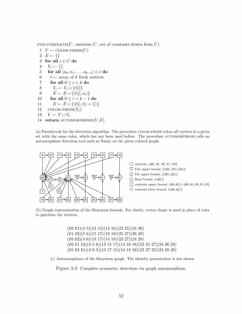
sym-complete(U : universe, C : set of constants drawn from U)1 V ← color-fresh(U)2 E ← {}3 for all c ∈ C do4 Vc ← {}5 for all 〈a0, a1, . . . , ak−1〉 ∈ c do6 t← array of k fresh vertices7 for all 0 ≤ i < k do8 Vc ← Vc ∪ {t[i]}9 E ← E ∪ {〈t[i], ai〉}

10 for all 0 ≤ i < k − 1 do11 E ← E ∪ {〈t[i], t[i + 1]〉}12 color-fresh(Vc)13 V ← V ∪ Vc

14 return automorphisms(V,E)

(a) Pseudocode for the detection algorithm. The procedure color-fresh colors all vertices in a givenset with the same color, which has not been used before. The procedure automorphisms calls anautomorphism detection tool such as Nauty on the given colored graph.

23

4 5 6d0 d1 f0 f1 f28

9 10 11 12 13 14 15 16 17 18

19 20 21 22 23 24 25 26 27 28

1

7

universe, {d0, d1, f0, f1, f2}File upper bound, {〈f0〉,〈f1〉,〈f2〉}Dir upper bound, {〈d0〉,〈d1〉}Root bound, {〈d0〉}contents upper bound, {d0, d1}×{d0, d1, f0, f1, f2}contents lower bound, {〈d0, d1〉}

(b) Graph representation of the filesystem bounds. For clarity, vertex shape is used in place of colorto partition the vertices.

(f0 f1)(4 5)(13 15)(14 16)(23 25)(24 26)(f1 f2)(5 6)(15 17)(16 18)(25 27)(26 28)(f0 f2)(4 6)(13 17)(14 18)(23 27)(24 28)(f0 f1 f2)(4 5 6)(13 15 17)(14 16 18)(23 25 27)(24 26 28)(f0 f2 f1)(4 6 5)(13 17 15)(14 18 16)(23 27 25)(24 28 26)

(c) Automorphisms of the filesystem graph. The identity permutation is not shown.

Figure 3-3: Complete symmetry detection via graph automorphism.

52

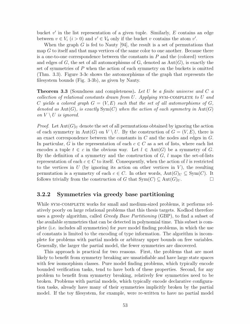
bucket v′ in the list representation of a given tuple. Similarly, E contains an edgebetween v ∈ Vi (i > 0) and v′ ∈ V0 only if the bucket v contains the atom v′.

When the graph G is fed to Nauty [94], the result is a set of permutations thatmap G to itself and that map vertices of the same color to one another. Because thereis a one-to-one correspondence between the constants in P and the (colored) verticesand edges of G, the set of all automorphisms of G, denoted as Aut(G), is exactly theset of symmetries of P when the action of each symmetry on the buckets is omitted(Thm. 3.3). Figure 3-3c shows the automorphisms of the graph that represents thefilesystem bounds (Fig. 3-3b), as given by Nauty.

Theorem 3.3 (Soundness and completeness). Let U be a finite universe and C acollection of relational constants drawn from U . Applying sym-complete to U andC yields a colored graph G = (V, E) such that the set of all automorphisms of G,denoted as Aut(G), is exactly Sym(C) when the action of each symmetry in Aut(G)on V \ U is ignored.

Proof. Let Aut(G)U denote the set of all permutations obtained by ignoring the actionof each symmetry in Aut(G) on V \ U . By the construction of G = (V, E), there isan exact correspondence between the constants in C and the nodes and edges in G.In particular, G is the representation of each c ∈ C as a set of lists, where each listencodes a tuple t ∈ c in the obvious way. Let l ∈ Aut(G) be a symmetry of G.By the definition of a symmetry and the construction of G, l maps the set-of-listsrepresentation of each c ∈ C to itself. Consequently, when the action of l is restrictedto the vertices in U (by ignoring its action on other vertices in V ), the resultingpermutation is a symmetry of each c ∈ C. In other words, Aut(G)U ⊆ Sym(C). Itfollows trivially from the construction of G that Sym(C) ⊆ Aut(G)U .

3.2.2 Symmetries via greedy base partitioning

While sym-complete works for small and medium-sized problems, it performs rel-atively poorly on large relational problems that this thesis targets. Kodkod thereforeuses a greedy algorithm, called Greedy Base Partitioning (GBP), to find a subset ofthe available symmetries that can be detected in polynomial time. This subset is com-plete (i.e. includes all symmetries) for pure model finding problems, in which the useof constants is limited to the encoding of type information. The algorithm is incom-plete for problems with partial models or arbitrary upper bounds on free variables.Generally, the larger the partial model, the fewer symmetries are discovered.

This approach is practical for two reasons. First, the problems that are mostlikely to benefit from symmetry breaking are unsatisfiable and have large state spaceswith few isomorphism classes. Pure model finding problems, which typically encodebounded verification tasks, tend to have both of these properties. Second, for anyproblem to benefit from symmetry breaking, relatively few symmetries need to bebroken. Problems with partial models, which typically encode declarative configura-tion tasks, already have many of their symmetries implicitly broken by the partialmodel. If the toy filesystem, for example, were re-written to have no partial model

53

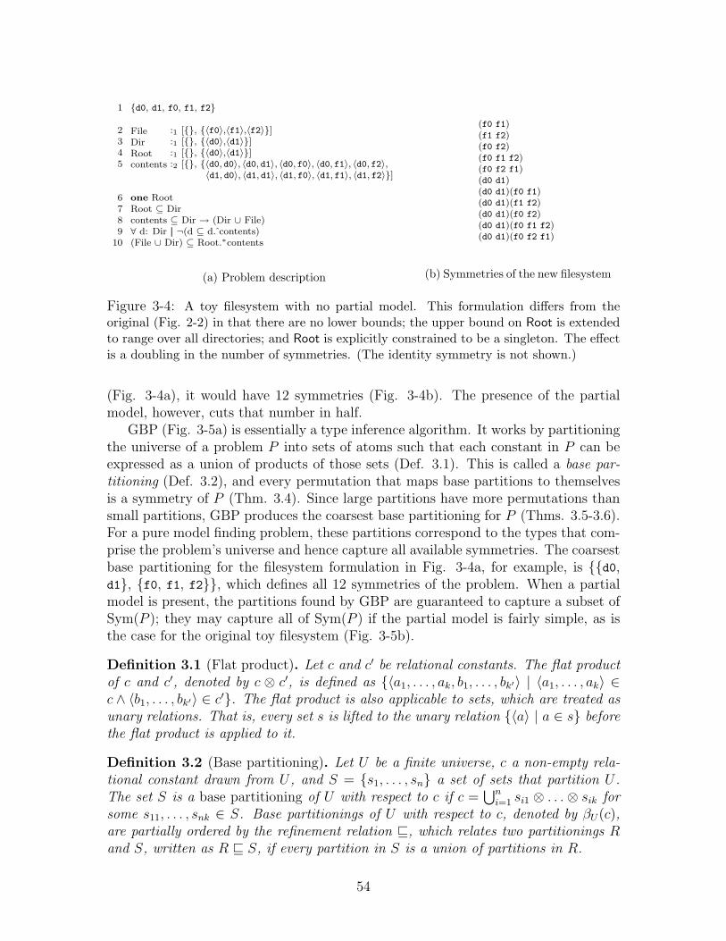
1 {d0, d1, f0, f1, f2}

2 File :1 [{}, {〈f0〉,〈f1〉,〈f2〉}]3 Dir :1 [{}, {〈d0〉,〈d1〉}]4 Root :1 [{}, {〈d0〉,〈d1〉}]5 contents :2 [{}, {〈d0, d0〉, 〈d0, d1〉, 〈d0, f0〉, 〈d0, f1〉, 〈d0, f2〉,

〈d1, d0〉, 〈d1, d1〉, 〈d1, f0〉, 〈d1, f1〉, 〈d1, f2〉}]

6 one Root7 Root ⊆ Dir8 contents ⊆ Dir → (Dir ∪ File)9 ∀ d: Dir || ¬(d ⊆ d. contents)

10 (File ∪ Dir) ⊆ Root.∗contents

(a) Problem description

(f0 f1)(f1 f2)(f0 f2)(f0 f1 f2)(f0 f2 f1)(d0 d1)(d0 d1)(f0 f1)(d0 d1)(f1 f2)(d0 d1)(f0 f2)(d0 d1)(f0 f1 f2)(d0 d1)(f0 f2 f1)

(b) Symmetries of the new filesystem

Figure 3-4: A toy filesystem with no partial model. This formulation differs from theoriginal (Fig. 2-2) in that there are no lower bounds; the upper bound on Root is extendedto range over all directories; and Root is explicitly constrained to be a singleton. The effectis a doubling in the number of symmetries. (The identity symmetry is not shown.)

(Fig. 3-4a), it would have 12 symmetries (Fig. 3-4b). The presence of the partialmodel, however, cuts that number in half.

GBP (Fig. 3-5a) is essentially a type inference algorithm. It works by partitioningthe universe of a problem P into sets of atoms such that each constant in P can beexpressed as a union of products of those sets (Def. 3.1). This is called a base par-titioning (Def. 3.2), and every permutation that maps base partitions to themselvesis a symmetry of P (Thm. 3.4). Since large partitions have more permutations thansmall partitions, GBP produces the coarsest base partitioning for P (Thms. 3.5-3.6).For a pure model finding problem, these partitions correspond to the types that com-prise the problem’s universe and hence capture all available symmetries. The coarsestbase partitioning for the filesystem formulation in Fig. 3-4a, for example, is {{d0,d1}, {f0, f1, f2}}, which defines all 12 symmetries of the problem. When a partialmodel is present, the partitions found by GBP are guaranteed to capture a subset ofSym(P ); they may capture all of Sym(P ) if the partial model is fairly simple, as isthe case for the original toy filesystem (Fig. 3-5b).

Definition 3.1 (Flat product). Let c and c′ be relational constants. The flat productof c and c′, denoted by c ⊗ c′, is defined as {〈a1, . . . , ak, b1, . . . , bk′〉 | 〈a1, . . . , ak〉 ∈c ∧ 〈b1, . . . , bk′〉 ∈ c′}. The flat product is also applicable to sets, which are treated asunary relations. That is, every set s is lifted to the unary relation {〈a〉 | a ∈ s} beforethe flat product is applied to it.

Definition 3.2 (Base partitioning). Let U be a finite universe, c a non-empty rela-tional constant drawn from U , and S = {s1, . . . , sn} a set of sets that partition U .The set S is a base partitioning of U with respect to c if c =

⋃ni=1 si1 ⊗ . . .⊗ sik for

some s11, . . . , snk ∈ S. Base partitionings of U with respect to c, denoted by βU(c),are partially ordered by the refinement relation v, which relates two partitionings Rand S, written as R v S, if every partition in S is a union of partitions in R.

54

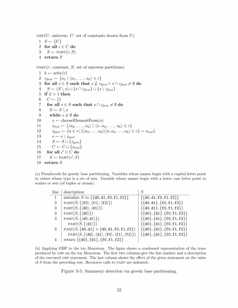
gbp(U : universe, C: set of constants drawn from U)1 S ← {U}2 for all c ∈ C do3 S ← part(c, S)4 return S

part(c: constant, S: set of universe partitions)1 k ← arity(c)2 cfirst ← {a1 | 〈a1, . . . , ak〉 ∈ c}3 for all s ∈ S such that s 6⊆ cfirst ∧ s ∩ cfirst 6= ∅ do4 S ← (S \ s) ∪ {s ∩ cfirst} ∪ {s \ cfirst}5 if k > 1 then6 C ← {}7 for all s ∈ S such that s ∩ cfirst 6= ∅ do8 S ← S \ s9 while s 6= ∅ do

10 x← chooseElementFrom(s)11 xrest ← {〈a2, . . . , ak〉 | 〈x, a2, . . . , ak〉 ∈ c}12 xpart ← {a ∈ s | {〈a2, . . . , ak〉|〈a, a2, . . . , ak〉 ∈ c} = xrest}13 s← s \ xpart

14 S ← S ∪ {xpart}15 C ← C ∪ {xrest}16 for all c′ ∈ C do17 S ← part(c′, S)18 return S

(a) Pseudocode for greedy base partitioning. Variables whose names begin with a capital letter pointto values whose type is a set of sets. Variable whose names begin with a lower case letter point toscalars or sets (of tuples or atoms).

line description S

1 initialize S to {{d0, d1, f0, f1, f2}} {{d0, d1, f0, f1, f2}}3 part(S, {〈f0〉, 〈f1〉, 〈f2〉}) {{d0, d1}, {f0, f1, f2}}3 part(S, {〈d0〉, 〈d1〉}) {{d0, d1}, {f0, f1, f2}}3 part(S, {〈d0〉}) {{d0}, {d1}, {f0, f1, f2}}3 part(S, {〈d0, d1〉}) {{d0}, {d1}, {f0, f1, f2}}

part(S, {〈d1〉}) {{d0}, {d1}, {f0, f1, f2}}3 part(S, {d0, d1} × {d0, d1, f0, f1, f2}) {{d0}, {d1}, {f0, f1, f2}}

part(S, {〈d0〉, 〈d1〉, 〈f0〉, 〈f1〉, 〈f2〉}) {{d0}, {d1}, {f0, f1, f2}}4 return {{d0}, {d1}, {f0, f1, f2}}

(b) Applying GBP to the toy filesystem. The figure shows a condensed representation of the traceproduced by gbp on the toy filesystem. The first two columns give the line number and a descriptionof the executed gbp statement. The last column shows the effect of the given statement on the valueof S from the preceding row. Recursive calls to part are indented.

Figure 3-5: Symmetry detection via greedy base partitioning.

55

Theorem 3.4 (Soundness). Let U be a finite universe, P a problem over U , andS = {s1, . . . , sn} a base partitioning of U with respect to the constants that occur inP . If a permutation l : U → U maps each s ∈ S to itself, then l ∈ Sym(P ).

Proof. Let c be a constant that occurs in P . Because l maps each partition in S toitself, and c is a union of products of some partitions in S, l(c) = c. This, by Thm.3.1, implies that l ∈ Sym(P ).

Theorem 3.5 (Local optimality of gbp). Let U be a finite universe and C a collectionof relational constants drawn from U . Applying gbp to U and C yields the coarsestbase partitioning of U with respect to C.

Proof. (by induction on the size of C). If C is empty, lines 2-3 of gbp never execute, sothe algorithm returns {U}. Suppose that C is non-empty, and let ci and Si designatethe values of the variables c and S at the end of the ith loop iteration. Since Sis initialized to {U}, S1 is, by Thm. 3.6, the coarsest base partitioning of U withrespect to c1. Suppose that Sn−1 is the coarsest base partitioning of U with respectto c1, . . . , cn−1. It follows from Def. 3.2 and the coarseness of Sn−1 that any basepartitioning of U with respect to c1, . . . , cn−1 must be a refinement of Sn−1. By Thm.3.6, Sn is the coarsest refinement of Sn−1 such that Sn ∈ βU(cn). Hence, Sn must bethe coarsest base partitioning of U with respect to c1, . . . , cn−1, cn.

Theorem 3.6 (Local optimality of part). Let U be a finite universe, c a relationalconstant drawn from U , and S a set of sets that partition U . Applying part to c andS yields the coarsest refinement of S that is a base partitioning of U with respect toc.

Proof. (by induction on the arity of c). Suppose that arity(c) = 1. Let S0 denote thevalue of S that is passed to the procedure, and let Sm denote the value of S afterthe first loop (lines 3-4) has terminated. Since an iteration of the loop simply splitsa partition s ∈ S0 into two partitions that add up to s, Sm v S0. The loop conditionensures that all partitions in Sm are either contained in c or do not intersect with it,so Sm ∈ βU(c). Finally, Sm is the coarsest refinement of S0 that is a base partitioningwith respect to c since none of the partitions created by the loop can be mergedwithout taking away one of the partitions that makes up c.

For the inductive case, suppose that the theorem holds for all constants of arityk − 1, and suppose that arity(c) = k. Let Sy denote the value of S after the secondloop (lines 7-15) has terminated; and let Sz be the value of S after the third loop(lines 16-17) has terminated. The first loop refines S0 into Sm, which is the coarsestbase partitioning of U with respect to the first column of c. The second loop splitseach s ∈ Sm that intersects with cfirst into the smallest number of subpartitions suchthat c maps all atoms in a subpartition, denoted by xpart , to the same constant ofarity k − 1, denoted by xrest . This ensures that Sy is the coarsest refinement of S0

such that c is a union of products of each xpart ∈ Sy \ Sm with its correspondingxrest ∈ C. By the inductive hypothesis, Sz is the coarsest refinement of Sy that is abase partitioning of U with respect to each xrest ∈ C. Hence, by Lemma 3.3, Sz isthe coarsest refinement of S0 that is a base partitioning of U with respect to c.

56

Lemma 3.3 (Partitioning invariant). Let U be a finite universe, c a constant of arityk > 1 drawn from U , and S a set of sets that partitions U . Let R be the coarsestrefinement of S such that c =

⋃ni=1 pi ⊗ ci for some distinct partitions p1, . . . , pn ∈ R

and some distinct constants c1, . . . , cn of arity k − 1. If Q is a refinement of S thatis a base partitioning with respect to c, then Q is a refinement of R that is a basepartitioning of U with respect to c1, . . . , cn.

Proof. The proof follows directly from Def. 3.2 and the definition of R.

3.3 Experimental results

Table 3.1 shows the results of applying gbp and symm-complete to a collection of 40benchmarks. Thirty are the Alloy and TPTP benchmarks introduced in the previouschapter. The remaining ten are drawn from a public database of graph coloringproblems [132]. The graphs to be colored are encoded as (large) partial models, andthe k-colorability problem for each graph is encoded as a relational formula over auniverse with k color atoms. All ten problems are unsatisfiable. The benchmarks inthe “mulsol” and “zeroin” families represent register allocation problems for variablesin real code; the “school” benchmarks are class scheduling problems.

The first two columns of Table 3.1 display the name of each benchmark and thesize of its partial model, given as the number of known tuples. The third columnshows the size of each problem’s state space, given as the number of bits neededto encode all possible bindings that extend the problem’s partial model (if any).The state space of AWD.A241, for example, consists of 22512 distinct bindings. The“GBP” and “Symm-Complete” columns display the time, in milliseconds, taken bythe corresponding algorithm to find the given number of symmetries, expressed in bits.The last two columns hold the SAT solving time for each problem, in milliseconds,with and without symmetry breaking. The notation “t/o” indicates that a givenprocess failed to produce a result within 5 minutes (300,000 ms).

All experiments were performed on a 2 × 3 GHz Dual-Core Intel Xeon with 2GB of RAM, using Kodkod’s translation algorithm to reduce the benchmarks to SATand MiniSat to solve the resulting boolean formulas. gbp is implemented as a part ofKodkod and works on the tool’s internal representation of relational constants as setsof integers. The symm-complete implementation converts each Kodkod constantto a graph and uses Nauty [94] for automorphism detection.3 Each benchmark wassolved twice, once without any symmetry breaking and once with a predicate basedon gbp’s output.

The resulting data illustrate the key points of this chapter: (1) many model find-ing and extension problems are infeasible without symmetry breaking; (2) completesymmetry detection is impractical for large problems; and (3) the subset of symme-tries detected by greedy base partitioning is sufficient for effective symmetry breaking.symm-complete timed out on 35% of the problems, and it was, on average, 8125times slower than gbp on the remaining ones. gbp found all symmetries for Alloy

3The more recent graph automorphism detection tools [28, 72] work only on undirected graphs.

57

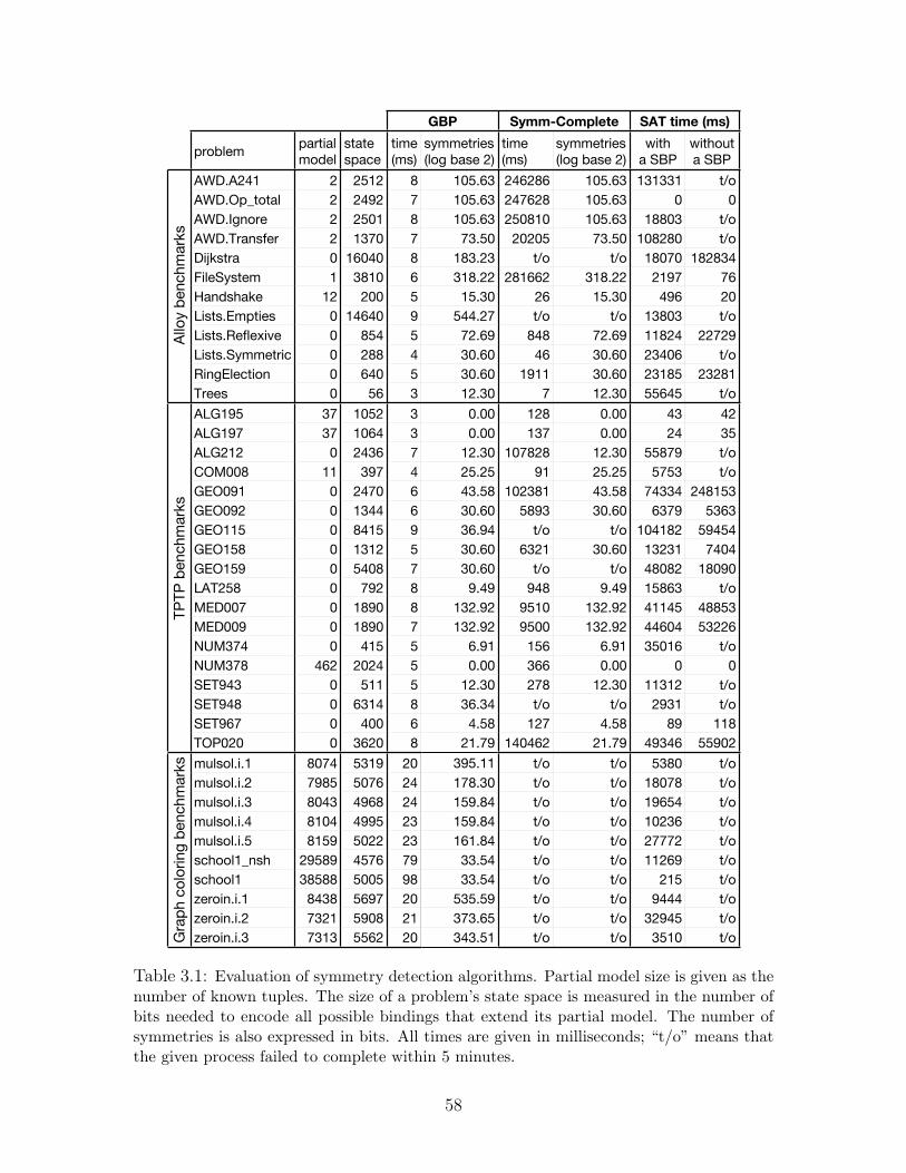
GBP Symm-Complete SAT time (ms)

problempartial

model

state

space

time

(ms)

symmetries

(log base 2)

time

(ms)

symmetries

(log base 2)

with

a SBP

without

a SBP

AWD.A241 2 2512 8 105.63 246286 105.63 131331 t/o

AWD.Op_total 2 2492 7 105.63 247628 105.63 0 0

AWD.Ignore 2 2501 8 105.63 250810 105.63 18803 t/o

AWD.Transfer 2 1370 7 73.50 20205 73.50 108280 t/o

Dijkstra 0 16040 8 183.23 t/o t/o 18070 182834

FileSystem 1 3810 6 318.22 281662 318.22 2197 76

Handshake 12 200 5 15.30 26 15.30 496 20

Lists.Empties 0 14640 9 544.27 t/o t/o 13803 t/o

Lists.Reflexive 0 854 5 72.69 848 72.69 11824 22729

Lists.Symmetric 0 288 4 30.60 46 30.60 23406 t/o

RingElection 0 640 5 30.60 1911 30.60 23185 23281

Trees 0 56 3 12.30 7 12.30 55645 t/o

ALG195 37 1052 3 0.00 128 0.00 43 42

ALG197 37 1064 3 0.00 137 0.00 24 35

ALG212 0 2436 7 12.30 107828 12.30 55879 t/o

COM008 11 397 4 25.25 91 25.25 5753 t/o

GEO091 0 2470 6 43.58 102381 43.58 74334 248153

GEO092 0 1344 6 30.60 5893 30.60 6379 5363

GEO115 0 8415 9 36.94 t/o t/o 104182 59454

GEO158 0 1312 5 30.60 6321 30.60 13231 7404

GEO159 0 5408 7 30.60 t/o t/o 48082 18090

LAT258 0 792 8 9.49 948 9.49 15863 t/o

MED007 0 1890 8 132.92 9510 132.92 41145 48853

MED009 0 1890 7 132.92 9500 132.92 44604 53226

NUM374 0 415 5 6.91 156 6.91 35016 t/o

NUM378 462 2024 5 0.00 366 0.00 0 0

SET943 0 511 5 12.30 278 12.30 11312 t/o

SET948 0 6314 8 36.34 t/o t/o 2931 t/o

SET967 0 400 6 4.58 127 4.58 89 118

TOP020 0 3620 8 21.79 140462 21.79 49346 55902

mulsol.i.1 8074 5319 20 395.11 t/o t/o 5380 t/o

mulsol.i.2 7985 5076 24 178.30 t/o t/o 18078 t/o

mulsol.i.3 8043 4968 24 159.84 t/o t/o 19654 t/o

mulsol.i.4 8104 4995 23 159.84 t/o t/o 10236 t/o

mulsol.i.5 8159 5022 23 161.84 t/o t/o 27772 t/o

school1_nsh 29589 4576 79 33.54 t/o t/o 11269 t/o

school1 38588 5005 98 33.54 t/o t/o 215 t/o

zeroin.i.1 8438 5697 20 535.59 t/o t/o 9444 t/o

zeroin.i.2 7321 5908 21 373.65 t/o t/o 32945 t/o

zeroin.i.3 7313 5562 20 343.51 t/o t/o 3510 t/o

Allo

y b

enchm

ark

sT

PT

P b

enchm

ark

sG

rap

h c

olo

ring

benchm

ark

s

Table 3.1: Evaluation of symmetry detection algorithms. Partial model size is given as thenumber of known tuples. The size of a problem’s state space is measured in the number ofbits needed to encode all possible bindings that extend its partial model. The number ofsymmetries is also expressed in bits. All times are given in milliseconds; “t/o” means thatthe given process failed to complete within 5 minutes.

58

and TPTP benchmarks, which are either pure model finding problems or have smallpartial models. It produced only a subset of the available symmetries4 for the graphcoloring benchmarks. Each of these subsets, however, captured enough symmetriesto enable MiniSat to solve the corresponding problem within the time limit.

3.4 Related work

Symmetry breaking has been extensively studied in both traditional model findingand in constraint programming. Most of the work on symmetries in traditional modelfinding has focused on the design of better symmetry breaking heuristics, dynamic andstatic. Detection of symmetries is performed implicitly by type inference algorithms.The first half of this section summarizes that work. The second half covers thework on symmetry breaking and detection in constraint programming. The latter isof particular interest since detecting symmetries of constraint programs is, in manyways, harder than detecting symmetries of both model finding and model extensionproblems.

3.4.1 Symmetries in traditional model finding

Most search-based model finders [70, 93, 122, 151, 152] use a variant of the LeastNumber Heuristic (LNH) [151] to reduce the number of isomorphic bindings that areexamined during search. The basic idea behind LNH is simple. At a given pointin the search, a type T is partitioned into elements {e1, . . . , ei} that appear in thecurrent partial assignment from variables to values and the elements {ei+1, . . . , en}that do not. The unconstrained elements, {ei+1, . . . , en}, are symmetric, so only one ofthem (e.g. ei+1) needs to be considered in the subsequent assignments. In particular,suppose that C is a set of (ground) first order clauses, A is a partial assignmentof variables constrained by C to values, and v is an unassigned variable of type T .To find a model of C in this scenario, it is sufficient to test only the bindings thatextend A with an assignment from v to an element in {e1, . . . , ei+1}. In practice, LNHimproves search times by orders of magnitude for many problems [152].

Unlike search-based model finders, SAT-based tools [25, 117] cannot exploit sym-metries dynamically. Instead, they employ a static symmetry breaking techniquethat involves augmenting the SAT encoding of a given problem with symmetrybreaking predicates. These are constraints that hold for at least one binding ineach isomorphism class in the problem’s state space. The lex-leader predicate [27],for example, is true only of the lexicographically smallest binding in an equiva-lence class. It has the form V ≤ l(V ), where l is a symmetry and V is an or-dering of the bits that make up the state space of a given problem. The formulad0d1f0f1f2c0c2c3c4c5c6c7c8c9 ≤ d0d1f1f0f2c0c3c2c4c5c6c8c7c9, for instance, is a lex-leader predicate for the symmetry (f0 f1) of the toy filesystem (Fig. 2-5). MostSAT-based model finders [25, 117] employ some variant of the lex-leader predicate.

4All ten graphs are undirected and have symmetries detectable with Bliss [72] that are notdetected by gbp.

59

Alloy3 and Kodkod use it in addition to predicates [116] that break symmetries onrelations with specific properties, such as acyclicity.

Model finders that accept typed formulas [69, 152, 117] use the provided sorts ortypes to identify symmetries. Those that accept untyped formulas take one of twoapproaches to symmetry detection. Mace4 [93] works on untyped problems directly,taking their symmetries to be all permutations of the universe of interpretation. Para-dox2.3 [25], on the other hand, first employs a sort inference algorithm to transforman untyped input problem into an equisatisfiable typed problem. It then solves thenew problem, taking its symmetries to be all permutations that respect the inferredtypes. The inference algorithm works as follows. First, it assigns unrelated sorts to allpredicate and function symbols that appear in a given set of unsorted clauses. Next,it forces all occurrences of a variable within a clause to have the same sort. Finally,it forces each pair of functions related by the ‘=’ symbol to have the same sort. Theresult is a sound typing (as defined in [70]) that can be applied to the input problemwithout affecting its satisfiability.

The process of typing unsorted problems, and then breaking symmetries on theresulting types, can lead to dramatic improvements in model finding performance.To see why, consider the problem P specified by the clause “∀x, f(x) 6= g(x),” wheref and g are uninterpreted functions with the universal typing f, g : U → U . In atwo atom universe {a0, a1}, P has 28 possible bindings since four bits are needed torepresent f and four to represent g. These bindings are partitioned into equivalenceclasses by two symmetries: (a0 a1) and the identity. Now consider the problem P ′

specified by the same clause as P but using the typing f : A → B and g : A →B inferred by Paradox2.3. In the universe {a0, a1, b0, b1} where each of the typeshas 2 atoms, P ′ has 28 bindings, like P , and it has a model only if P does. Thekey difference between the two is that P ′ has twice as many symmetries as P , i.e.(a0 a1), (b0 b1), (a0 a1)(b0 b1), and the identity. Since more symmetries lead to fewerisomorphism classes, a model finder needs to examine half as many (representative)bindings to solve P ′ as it does to solve P .

3.4.2 Symmetries in constraint programming

As in traditional model finding, symmetry breaking methods used in constraint pro-gramming fall into two categories: static and dynamic. Static approaches include anumber of predicates based on the lex-leader method (e.g. [47, 50, 104]). Dynamicapproaches include Symmetry Breaking During Search [10, 11], Symmetry Breakingvia Dominance Detection [45, 48], and Symmetry Breaking Using Stabilizers [103].Gent et al. [55] provide a detailed overview of these techniques, both static anddynamic.

The research on the identification of symmetries in constraint solving problems(CSPs) has focused mostly on methods [54, 64] for enabling the user to specify com-monly occurring symmetries directly, such as “all rows of the matrix m can be inter-changed.” Detecting the symmetries of a CSP automatically is tricky for two reasons.First, there are nearly a dozen different definitions of a symmetry for a CSP [26, 55].Of these, the most liberal definition is that of a solution symmetry [26], defined as a

60

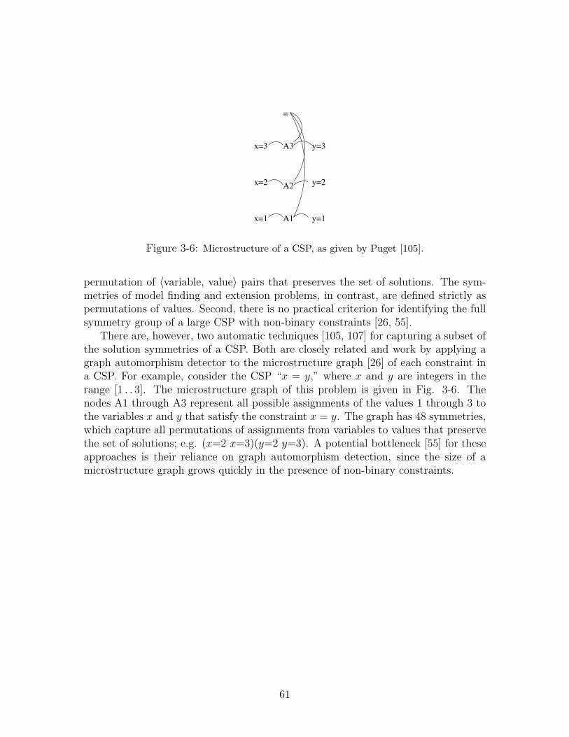
Automatic Detection of Variable and Value Symmetries 485

y=1

x=2

x=1 A1

A2

A3

=

y=3

y=2

x=3

(a) Equality

y=3x=3

x=1 A1

A2

A3

<

y=1

y=2x=2

(b) Inequality

y=2g=5

g=4

g=3

g=2

g=1 A1

A2

A3

A4

A5

A6 y=3

game

x=1

x=2

x=3

y=1

g=6

(c) Game

Fig. 6. Some symmetry graphs

If the number of variables is equal to the number of values, then the constraintcan be stated by

!j!

i

yij = 1 (5)

Then, depending on the case the vertices and edges for equation (4) or (5) areadded.

Example 12. Let us consider the global cardinality constraint gcc(X, C, V )where X is a vector of variables < x1, . . . , xn >, C another vector of variables< c1, . . . , cm >, and V a vector of values < v1, . . . , vm >. Let yij be the variablescorresponding to the values of the xi variables, and let zkl be the variablescorresponding to the values of the ck variables. Then the gcc constraint can beexpressed by:

!j!

i

yij =!

l

l " zjl (6)

Indeed, we have that"

i yij = cj and that ck ="

l l"zkl. Therefore, the verticesan edges corresponding to (6) are added.

5.3 Handling Expressions

The treatment of expressions is more complex. Indeed, one needs to be able toexpress the relationship between value vertices of x op y and the value vertices ofx and y. A generic way is to replace expressions by constraints. For instance, anexpression x op y where op is a binary operator can be replaced by a new variable zand a ternary constraint op(z, x, y). Then this ternary constraint can be describedin extension. This approach is correct: any symmetry of the resulting graph is asymmetry of the CSP. However, it may lead to extremely large graphs.

We have decided to only handle some simple expressions when detecting allsymmetries. We handle expressions f(x) involving only one occurrence of onevariable x. Let yj be the vertices representing x = j. Then the only possible

Figure 3-6: Microstructure of a CSP, as given by Puget [105].

permutation of 〈variable, value〉 pairs that preserves the set of solutions. The sym-metries of model finding and extension problems, in contrast, are defined strictly aspermutations of values. Second, there is no practical criterion for identifying the fullsymmetry group of a large CSP with non-binary constraints [26, 55].

There are, however, two automatic techniques [105, 107] for capturing a subset ofthe solution symmetries of a CSP. Both are closely related and work by applying agraph automorphism detector to the microstructure graph [26] of each constraint ina CSP. For example, consider the CSP “x = y,” where x and y are integers in therange [1 . . 3]. The microstructure graph of this problem is given in Fig. 3-6. Thenodes A1 through A3 represent all possible assignments of the values 1 through 3 tothe variables x and y that satisfy the constraint x = y. The graph has 48 symmetries,which capture all permutations of assignments from variables to values that preservethe set of solutions; e.g. (x=2 x=3)(y=2 y=3). A potential bottleneck [55] for theseapproaches is their reliance on graph automorphism detection, since the size of amicrostructure graph grows quickly in the presence of non-binary constraints.

61

62

Chapter 4

Finding Minimal Cores

A specification that has no models in a given universe is said to be unsatisfiable in thatuniverse. Most model finders offer no feedback on unsatisfiable specifications apartfrom reporting that no models were found. But many applications need to knowthe cause of a specification’s unsatisfiability, either to take corrective action (in thecase of declarative configuration [133]) or to check that no models exist for the rightreasons (in the case of bounded verification [31, 21]). In bounded verification [31, 21],for example, unsatisfiability is a necessary but insufficient indicator of success. If theverification formula s1 ∧ . . .∧ sn ∧¬p has a model, such a model is a witness that thesystem described by s1 ∧ . . .∧ sn violates the property p. But a lack of models is nota guarantee of success. If the formula is unsatisfiable because the system descriptions1 ∧ . . . ∧ sn is overconstrained, or because p is a tautology, then the analysis isconsidered to have failed due to a ‘vacuity’ error.

A cause of unsatisfiability of a given specification is called an unsatisfiable core.It is expressed as a subset of the specification’s constraints that is itself unsatisfiable.Every such subset includes one or more critical constraints that cannot be removedwithout making the remainder of the core satisfiable. Non-critical constraints, if any,are irrelevant to unsatisfiability and generally decrease a core’s utility both for diag-nosing faulty configurations [133] and for checking the results of a bounded analysis[129]. Cores that include only critical constraints are said to be minimal.

This chapter presents a new technique for extracting minimal unsatisfiable cores,called recycling core extraction (RCE). The technique was developed in the context ofSAT-based model finding and relies on the ability of modern SAT solvers to producecheckable proofs of unsatisfiability. It is, however, more generally applicable. Therest of this chapter therefore describes RCE in broader terms, as a technique forextracting minimal cores of specifications that are translatable to the input logic ofsome resolution engine (e.g. a SAT solver or a resolution-based theorem prover). Thetechnique is shown to be sound, minimal, and effective in practice. Its effectiveness isevaluated on a set of benchmarks of varying difficulties, where the difficulty of findinga minimal core is given as a function of its size, the size of the overall problem, and thetime taken (by a resolution engine) to prove that the overall problem is unsatisfiable.

63

4.1 A small example

The first chapter demonstrated the use of minimal cores for diagnosis and repair of afaulty Sudoku configuration. This section shows how they can be used to expose threekinds of coverage errors that commonly arise in bounded verification: overconstrainingthe system description, so that legitimate behaviors are excluded; checking the systemagainst a weak property, so that bad behaviors are accepted; and setting the analysisbounds too small, so that the model finder does not examine a sufficiently large spaceof possibilities. The last problem is specific to bounded verification and is not sufferedby analyses based on theorem provers. These analyses are not immune to the firsttwo problems, however, so the techniques presented here will work for them too.

4.1.1 A toy list specification

As an example, consider the toy formalization of LISP-style lists given in Fig. 4-1.There are two distinct kinds of lists (lines 10-11): cons cells and nil lists. Nil lists donot have any structure. A cons cell, on the other hand, is defined by two functions,car and cdr. The car function maps each cons cell to the thing stored in that cell (lines12-13). The cdr function maps it to the rest of the list (lines 14-15). Every list endswith a Nil list (line 16).

The equivTo (line 17) and prefixes (line 19) relations define what it means for twolists to be equivalent to each other and what it means for one list to be a prefix ofanother. The equivalence definition is simple. Two lists are equivalent only if theystore the same thing and have equivalent tails (line 18). The prefix definition consistsof three constraints. First, a nil list is a prefix of every list (line 20); second, a conscell is never a prefix of a nil list (line 21); and third, one cons cell is a prefix of anotheronly if the two store the same thing and the tail of the first cell is a prefix of the tailof the second cell (line 22).

The universe in which the toy list specification is analyzed generally depends onthe property being checked. The universe and bounds declarations in Fig. 4-1 showa sample analysis set-up involving three lists and three things. All relations haveempty lower bounds, and their upper bounds reflect their types. List, Nil and Cons

all range over the list atoms (lines 2-4). The upper bound on Thing consists of the“thing” atoms (line 5). The binary relation car is bound above by the cross productof lists and things (line 6). The remaining relations all range over the cross productof list atoms with themselves (line 7-9).

4.1.2 Sample analyses

Bounded verification of a system against a given property involves checking that theconjunction of the system constraints and the negation of the property is unsatisfiable.The check is performed within a user-provided finite scope, i.e. a finite universe anda corresponding set of bounds on free variables. If the property is invalid in thegiven scope, a model finder will produce a counterexample. This is a model of theverification formula, and, as such, it represents a behavior of the system that violates

64

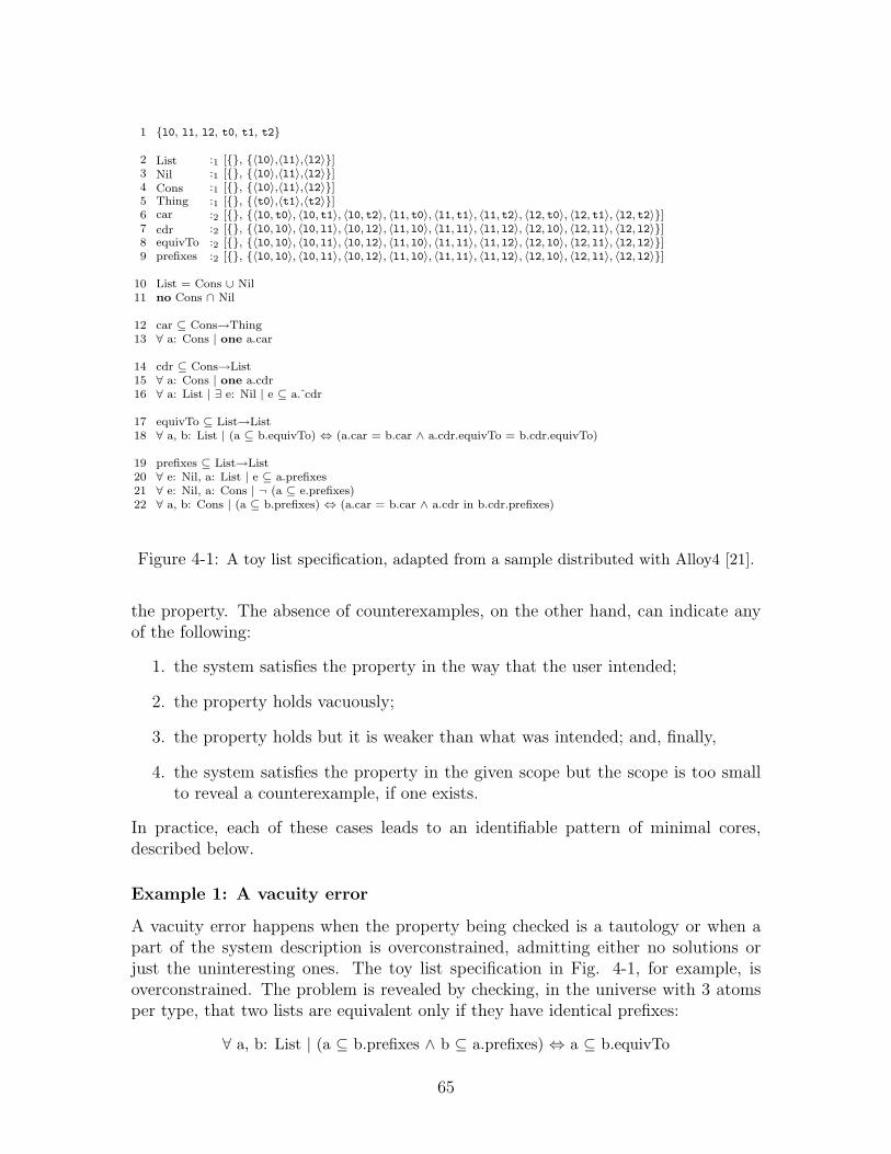
1 {l0, l1, l2, t0, t1, t2}

2 List :1 [{}, {〈l0〉,〈l1〉,〈l2〉}]3 Nil :1 [{}, {〈l0〉,〈l1〉,〈l2〉}]4 Cons :1 [{}, {〈l0〉,〈l1〉,〈l2〉}]5 Thing :1 [{}, {〈t0〉,〈t1〉,〈t2〉}]6 car :2 [{}, {〈l0, t0〉, 〈l0, t1〉, 〈l0, t2〉, 〈l1, t0〉, 〈l1, t1〉, 〈l1, t2〉, 〈l2, t0〉, 〈l2, t1〉, 〈l2, t2〉}]7 cdr :2 [{}, {〈l0, l0〉, 〈l0, l1〉, 〈l0, l2〉, 〈l1, l0〉, 〈l1, l1〉, 〈l1, l2〉, 〈l2, l0〉, 〈l2, l1〉, 〈l2, l2〉}]8 equivTo :2 [{}, {〈l0, l0〉, 〈l0, l1〉, 〈l0, l2〉, 〈l1, l0〉, 〈l1, l1〉, 〈l1, l2〉, 〈l2, l0〉, 〈l2, l1〉, 〈l2, l2〉}]9 prefixes :2 [{}, {〈l0, l0〉, 〈l0, l1〉, 〈l0, l2〉, 〈l1, l0〉, 〈l1, l1〉, 〈l1, l2〉, 〈l2, l0〉, 〈l2, l1〉, 〈l2, l2〉}]

10 List = Cons ∪ Nil11 no Cons ∩ Nil

12 car ⊆ Cons→Thing13 ∀ a: Cons | one a.car

14 cdr ⊆ Cons→List15 ∀ a: Cons | one a.cdr16 ∀ a: List | ∃ e: Nil | e ⊆ a. cdr

17 equivTo ⊆ List→List18 ∀ a, b: List | (a ⊆ b.equivTo) ⇔ (a.car = b.car ∧ a.cdr.equivTo = b.cdr.equivTo)

19 prefixes ⊆ List→List20 ∀ e: Nil, a: List | e ⊆ a.prefixes21 ∀ e: Nil, a: Cons | ¬ (a ⊆ e.prefixes)22 ∀ a, b: Cons | (a ⊆ b.prefixes) ⇔ (a.car = b.car ∧ a.cdr in b.cdr.prefixes)

Figure 4-1: A toy list specification, adapted from a sample distributed with Alloy4 [21].

the property. The absence of counterexamples, on the other hand, can indicate anyof the following:

1. the system satisfies the property in the way that the user intended;

2. the property holds vacuously;

3. the property holds but it is weaker than what was intended; and, finally,

4. the system satisfies the property in the given scope but the scope is too smallto reveal a counterexample, if one exists.

In practice, each of these cases leads to an identifiable pattern of minimal cores,described below.

Example 1: A vacuity error

A vacuity error happens when the property being checked is a tautology or when apart of the system description is overconstrained, admitting either no solutions orjust the uninteresting ones. The toy list specification in Fig. 4-1, for example, isoverconstrained. The problem is revealed by checking, in the universe with 3 atomsper type, that two lists are equivalent only if they have identical prefixes:

∀ a, b: List | (a ⊆ b.prefixes ∧ b ⊆ a.prefixes) ⇔ a ⊆ b.equivTo

65

Kodkod confirms that the property has no counterexamples in the given scope,and produces the following minimal core:

11 no Cons ∩ Nil14 cdr ⊆ Cons→List16 ∀ a: List | ∃ e: Nil | e ⊆ a. cdr23 ¬(∀ a, b: List | (a ⊆ b.prefixes ∧ b ⊆ a.prefixes) ⇔ a ⊆ b.equivTo)

Increasing the analysis scope to a universe and bounds with 5, 10 or 20 atoms ofeach type yields the same result. Neither the definition of prefixes nor equivalence isneeded to prove the property. Why?

Examining the core more closely reveals that the constraint on line 16 is toostrong. It says that, for every list, traversing the cdr pointer one or more times leadsto some nil list. But nil lists have no tails (lines 11 and 14). Consequently, there areno lists, nil or otherwise, that satisfy the toy list description. That is, the specificationis consistent, but it only admits trivial models in which the List relation is empty. Arevised definition of what it means for a list to be nil-terminated is given below:

16 ∀ a: List | ∃ e: Nil | e ⊆ a.∗cdr

It states that, for every list, traversing the cdr pointer zero or more times leads tosome nil list.

Example 2: A successful analysis

Checking a valid system description against a strong property results in minimal coresthat include the negation of the property and most of the system constraints. Whenthe revised toy list is checked against the previous assertion, Kodkod, once again,finds no counterexamples in the scope of 3 atoms per type. But the extracted corenow includes the negation of the property and the constraints on lines 12, 14, 16,18, and 20-22. When the scope is increased to 5 atoms per type, this core grows toinclude the constraint on line 17. Further increases in scope (e.g. up to 9 atoms pertype) have no effect on the contents of the extracted core, suggesting that the toy listsatisfies the property as intended.

Example 3: A weak property

A valid assertion that exercises only a small portion of a system is said to be weak.By themselves, weak assertions are not harmful, but they can be misleading. If thesystem analyst believes that a weak assertion covers all or most of the system, he canmiss real errors in the parts of the system that are not exercised. For example, thefollowing property is supposed to exercise both equivalence and prefix definitions. Itstates that a list which is equivalent to all of its prefixes has a nil tail:

∀ a: List | (a.prefixes = a.equivTo) ⇒ a.cdr ⊆ Nil

Kodkod verifies the property against the revised specification in the scope of 3atoms per type, producing the following minimal core:

66

11 no Cons ∩ Nil14 cdr ⊆ Cons→List16 ∀ a: List | ∃ e: Nil | e ⊆ a.∗cdr18 ∀ a, b: List | (a ⊆ b.equivTo) ⇔ (a.car = b.car ∧ a.cdr.equivTo = b.cdr.equivTo)20 ∀ e: Nil, a: List | e ⊆ a.prefixes23 ¬(∀ a: List | (a.prefixes = a.equivTo) ⇒ a.cdr ⊆ Nil)

The tool’s output remains the same as the scope is increased to 5, 10 and 20 atomsper type. This is problematic because it shows that the property exercises only oneconstraint in the prefix definition, when the intention was to exercise the definitionin its entirety. In other words, the property was intended to fail if any part of theprefix definition was wrong, but it will, in fact, hold even if the constraints on lines21 and 22 are replaced with the constant “true.”

Example 4: An insufficient scope

Many properties require a certain minimum scope for a bounded analysis to be mean-ingful. If a property applies only to lists of length 3 or more, establishing that it holdsfor lists with fewer than 3 elements is not useful. But determining a minimum usefulscope can be tricky. Consider, for example, the following property, which states thatthe prefix relation is transitive over cons cells:

∀ a, b, c: Cons | (a ⊆ b.prefixes ∧ b ⊆ c.prefixes) ⇒ a ⊆ c.prefixes

Since the property includes three quantified variables, it seems that 3 atoms pertype should be the minimum useful scope for checking the property against the revisedlist specification. The corresponding core, however, shows that either this scope orthe property is insufficient to cover the prefix definition:

15 ∀ a: Cons | one a.cdr16 ∀ a: List | ∃ e: Nil | e ⊆ a.∗cdr19 prefixes ⊆ List→List21 ∀ e: Nil, a: Cons | ¬ (a ⊆ e.prefixes)22 ∀ a, b: Cons | (a ⊆ b.prefixes) ⇔ (a.car = b.car ∧ a.cdr in b.cdr.prefixes)23 ¬(∀ a, b, c: Cons | (a ⊆ b.prefixes ∧ b ⊆ c.prefixes) ⇒ a ⊆ c.prefixes)

When the analysis is repeated in the scope of 4 atoms per type, the core increasesto include the rest of the prefix definition (line 20), demonstrating that the propertyis strong enough but that the scope of 3 is too small. This makes sense. Becauseevery list must be nil-terminated, at least four lists are needed to check the propertyagainst a scenario in which the variables a, b and c are bound to distinct cons cells.Moreover, the core remains the same as the scope is increased (up to 8 atoms pertype), suggesting that 4 atoms per type is indeed the minimum useful scope.

67

4.2 Core extraction with a resolution engine

The core extraction facility featured in the previous section implements a new tech-nique for finding minimal cores, called recycling core extraction (RCE). RCE relieson the ability of modern SAT solvers to produce checkable proofs of unsatisfiability,expressed as DAGs. These proofs encode inferences made by the solver that leadfrom a subset, or a core, of the input clauses to a contradiction. Exploiting SATproofs, however, is challenging because their cores are not guaranteed to be mini-mal or even small. Moreover, mapping a small boolean core back to specificationconstraints—a technique called one-step core extraction (OCE) [118]—may still yielda large specification-level core. Shlyakhter [117], for example, found that reducingthe size of the boolean core prior to mapping it back had little to no effect on the sizeof the resulting specification-level core.

RCE is based on two key ideas. The first idea is to minimize the core at thespecification rather than the boolean level. That is, the initial boolean core is mappedto a specification level core, which is then pruned by removing candidate constraintsand testing the remainder for satisfiability. The second idea is to use the booleanproof, and the mapping between the specification constraints and the translationclauses, to identify the inferences made by the solver that are still valid when aspecification-level constraint is removed. By adding these inferences (expressed asclauses) to the translation of a candidate core, RCE allows the solver to reuse thework from previous invocations.

Although RCE was developed in the context of SAT-based model finding for rela-tional logic, the technique is more widely applicable. This section therefore presentsthe RCE algorithm, and the proofs of its soundness and minimality, in the context ofan abstract resolution-based analysis framework. The framework captures the generalstructure of SAT solvers [43, 56, 87], SAT-based model finders [25, 117, 131], andresolution-based theorem provers [74, 108, 145]. Abstractly, they all work by trans-lating a declarative specification to a clausal logic and applying a resolution procedureto the resulting clauses.1 The framework provides a high-level formalization of thekey properties of these specifications, translations, and resolution engines.

4.2.1 Resolution-based analysis

Resolution [109] is a complete technique for proving that a set of clauses is unsatis-fiable. It involves the application of the resolution rule (Fig. 4-2) to a set of clausesuntil the empty clause is derived, indicating unsatisfiability, or until no more clausescan be derived, indicating satisfiability. This process is guaranteed to terminate onan unsatisfiable input with a proof of its unsatisfiability, which takes the form of aresolution refutation graph (Def. 4.1). Its behavior on satisfiable inputs depends onthe decidability of the underlying logic. SAT solvers, for example, are resolution en-gines (Def. 4.2) for propositional logic, which is decidable, and they will terminate onevery set of propositional clauses given enough time. Theorem provers, on the other

1SAT solvers can be viewed as using the identity as their translation function.

68

hand, will run forever on some inputs since first order logic is undecidable.

SAT solvers are unique among resolution-based tools in that their input languageis a clausal logic. Other tools that are based on resolution, such as theorem proversand model finders, accept syntactically richer languages, which they translate to firstorder or propositional clauses. The details of these languages and their translationsdiffer from one tool to another, but they all share two basic properties. First, theinput of each tool is a set of declarative constraints, or a specification (Def. 4.3), whichis tested for unsatisfiability in some implicit or explicit universe of values. Second,translations employed by resolution-based tools are regular (Def. 4.4). That is, aspecification and its translation are either both satisfiable or both unsatisfiable; thetranslation of a specification is the union of the clauses produced for each constraint;and the clauses produced for a given constraint in the context of different specificationsare the same, up to a renaming of identifiers (i.e. variable, constant, predicate andfunction names).

Figure 4-3 shows an example of a resolution-based analysis of the specification(a⇔ b)∧(b⇔ c)∧¬(a⇒ c). The specification is encoded in non-clausal propositionallogic, and the translation T applies standard inference rules to transform this languageto clauses. It is easy to see that both the specification and the translation satisfythe definitions 4.3 and 4.4. Because the specification is unsatisfiable, feeding itstranslation to the resolution engine E produces a proof of unsatisfiability in the formof a resolution refutation graph. The nodes of the graph are the translation clausesand the resolvent clauses inferred by the engine. The edges denote the applicationof the resolution rule. For example, the edges incident to ¬b indicate that ¬b is theresult of applying the resolution rule to the clauses ¬b ∨ c and ¬c. The translationclauses that are connected to the empty clause c∅ form an unsatisfiable core of thetranslation.

Definition 4.1 (Resolution refutation). Let C and R be sets of clauses such that R\Ccontains the empty clause, denoted by c∅. A directed acyclic graph G = (C, R, E) isa resolution refutation of C iff

1. each r ∈ R is the result of resolving some clauses x1, . . . , xn ∈ C ∪R;

2. the only edges in E are 〈x1, r〉, . . . , 〈xn, r〉 for each r ∈ R; and,

3. c∅ is the sink of G.

The sources of G are denoted by {c ∈ C | c∅ ∈ E∗LcM}, where E∗ is the reflexivetransitive closure of E and E∗LcM is the relational image of c under E∗. These forman unsatisfiable core of C.

Definition 4.2 (Resolution engine). A resolution engine E : P(C) ⇀ G is a partialfunction that maps each unsatisfiable clause set C to a resolution refutation graphG = (C, R, E). The remaining clause sets on which E is defined are taken to resolutiongraphs that do not include c∅, indicating satisfiability.

69

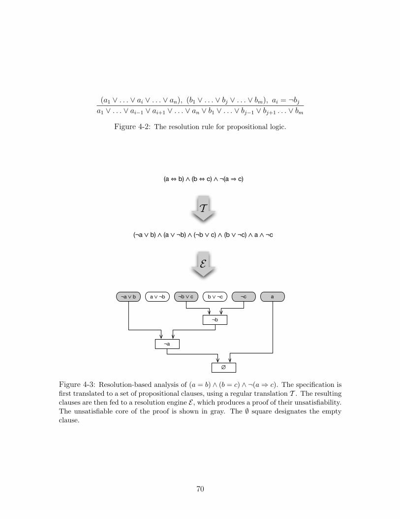
(a1 ∨ . . . ∨ ai ∨ . . . ∨ an), (b1 ∨ . . . ∨ bj ∨ . . . ∨ bm), ai = ¬bj

a1 ∨ . . . ∨ ai−1 ∨ ai+1 ∨ . . . ∨ an ∨ b1 ∨ . . . ∨ bj−1 ∨ bj+1 . . . ∨ bm

Figure 4-2: The resolution rule for propositional logic.

¬c a

¬b

¬a

∅

a ∨ ¬b¬a ∨ b ¬b ∨ c b ∨ ¬c

(a ⇔ b) ∧ (b ⇔ c) ∧ ¬(a ⇒ c)

(¬a ∨ b) ∧ (a ∨ ¬b) ∧ (¬b ∨ c) ∧ (b ∨ ¬c) ∧ a ∧ ¬c

T

E

Figure 4-3: Resolution-based analysis of (a = b) ∧ (b = c) ∧ ¬(a⇒ c). The specification isfirst translated to a set of propositional clauses, using a regular translation T . The resultingclauses are then fed to a resolution engine E , which produces a proof of their unsatisfiability.The unsatisfiable core of the proof is shown in gray. The ∅ square designates the emptyclause.

70

Definition 4.3 (Declarative specification). A declarative specification S is a set ofconstraints {s1, . . . , sn}, interpreted in a universe of values U .2 That is, all identifiersthat appear in S denote either values from U or variables that range over U . Theconstraints si ∈ S represent boolean functions whose conjunction is the meaning of Sas a whole.

Definition 4.4 (Regular translation). A procedure T : L → P(C) is a regular trans-lation of specifications in the language L to the clausal logic P(C) iff

1. a specification S ∈ L is unsatisfiable whenever T (S) is unsatisfiable;

2. the translation of a specification S ∈ L is the union of the translations of its con-straints: T (S) = TS(roots(S)) = ∪s∈roots(S)TS(s), where TS(s) is the translationof the constraint s in the context of the specification S; and,

3. the translation of the constraints S ′ ⊆ S is context independent up to a renam-ing: TS(S ′) = r(T (S ′)) for some bijection r from the identifiers that occur inTS(S ′) to those that occur in T (S ′), lifted to clauses and sets of clauses in theobvious way.

4.2.2 Recycling core extraction

Recycling core extraction is closely related to three simpler techniques: naive, one-step, and simple core extraction (NCE, OCE, and SCE). NCE and OCE have beendescribed in previous work, the former for propositional logic [32] and linear programs[23] and the latter for declarative languages reducible to SAT [118]. SCE is a newtechnique that combines NCE and OCE, and RCE is a refinement of SCE. Thepseudo-code for all four algorithms is shown in Fig. 4-4.

NCE (Fig. 4-4a) is the most basic method for extracting minimal cores in that ituses the resolution engine solely for satisfiability testing. The algorithm starts withan initial core K that contains the entire specification (line 1). The initial core isthen pruned, one constraint at a time, by discarding all constraints u for which aregular translation of K \ {u} is unsatisfiable (lines 3-8). This pruning step is soundsince the regularity of the translation guarantees that T (K \ {u}) and K \ {u} areequisatisfiable. In the end, K contains a minimal core of S.

Because it calls the resolution procedure once for each constraint, NCE tendsto be impractical for large specifications with small, hard cores. Shlyakhter et al.[118] addressed this problem with OCE (Fig. 4-4b), which sacrifices minimality forscalability. OCE simply returns all constraints in S whose translation contributesclauses to the unsatisfiable core of E(T (S)). The set of constraints computed in thisway is an unsatisfiable core of S (§4.2.3), but it is usually not minimal.

SCE (Fig. 4-4c) combines the pruning loop of NCE with the extraction step ofOCE. In particular, SCE is NCE with the following modifications: initialize K with

2The term ‘universe of values’ refers to all possible values that the variables in a specificationcan take. For example, in the case of bounded relational logic, the ‘universe of values,’ as opposedto the ‘universe of atoms,’ refers to the entire state space of a specification.

71

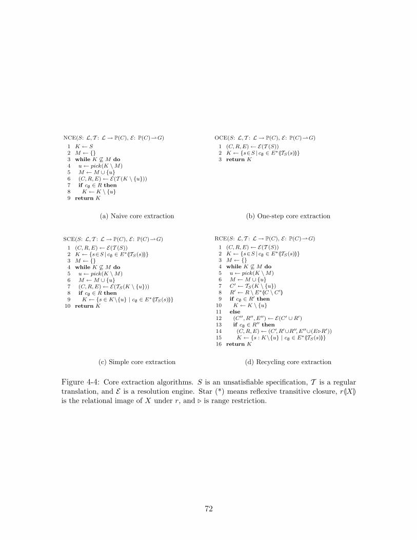
NCE(S: L, T : L → P(C), E: P(C)⇀G)

1 K ← S2 M ← {}3 while K 6⊆M do4 u← pick(K \M)5 M ←M ∪ {u}6 (C, R, E)← E(T (K \ {u}))7 if c∅ ∈ R then8 K ← K \ {u}9 return K

(a) Naive core extraction

OCE(S: L, T : L → P(C), E: P(C)⇀G)

1 (C, R, E)← E(T (S))2 K ← {s∈S | c∅ ∈ E∗LTS(s)M}3 return K

(b) One-step core extraction

SCE(S: L, T : L → P(C), E: P(C)⇀G)

1 (C, R, E)← E(T (S))2 K ← {s∈S | c∅ ∈ E∗LTS(s)M}3 M ← {}4 while K 6⊆M do5 u← pick(K \M)6 M ←M ∪ {u}7 (C, R, E)← E(TS(K \ {u}))8 if c∅ ∈ R then9 K ← {s ∈ K\{u} | c∅ ∈ E∗LTS(s)M}

10 return K

(c) Simple core extraction

RCE(S: L, T : L → P(C), E: P(C)⇀G)

1 (C, R, E)← E(T (S))2 K ← {s∈S | c∅ ∈ E∗LTS(s)M}3 M ← {}4 while K 6⊆M do5 u← pick(K \M)6 M ←M ∪ {u}7 C′ ← TS(K \ {u})8 R′ ← R \ E∗LC \ C′M9 if c∅ ∈ R′ then

10 K ← K \ {u}11 else12 (C′′, R′′, E′′)← E(C′ ∪R′)13 if c∅ ∈ R′′ then14 (C, R, E)← (C′, R′∪R′′, E′′∪(E.R′))15 K ← {s : K\{u} | c∅ ∈ E∗LTS(s)M}16 return K

(d) Recycling core extraction

Figure 4-4: Core extraction algorithms. S is an unsatisfiable specification, T is a regulartranslation, and E is a resolution engine. Star (*) means reflexive transitive closure, rLXMis the relational image of X under r, and . is range restriction.

72

a core of S instead of S (line 2), and reduce K to a core of K \ {u} instead ofK \{u} in the iterative step (line 9). These modifications eliminate unnecessary callsto the resolution engine without affecting either the soundness or the minimality ofthe resulting core (§4.2.3). But they still do not eliminate all unnecessary work. Byapplying E solely to TS(K \ {u}) on line 7, SCE forces the engine to re-learn some orall the clauses that it has already learned about TS(K \ {u}) while refuting TS(K).

RCE (Fig. 4-4d) extends SCE with a mechanism for reusing learned clauses.Line 7 of RCE constructs T (K \ {u}) from the already computed translations ofthe constraints in S, and line 8 collects the resolvents that E had already learnedabout T (K \ {u}). These are simply all resolvents reachable from T (K \ {u}) butnot from the other clauses previously fed to E . If they include the empty clausec∅, u is discarded (line 10) because there must be some other constraint in K \ {u}whose translation contributes the same or a larger set of clauses to the core of C asu. Otherwise, line 12 applies E to T (K \ {u}) and its resolvents. If the result is arefutation, the invalidity of K can be proved without u. The core of (C ′′, R′′, E ′′),however, does not necessarily correspond to a core of S because the former mayinclude resolvents for T (K \ {u}). Consequently, lines 14-15 fix the proof and set Kto the corresponding core, which excludes at least u.

4.2.3 Correctness and minimality of RCE

The soundness and minimality of SCE and RCE are proved below. Theorem 4.1establishes that the step they share with OCE is sound. This is then used in the proofof Thm. 4.2 to show that, if it terminates, RCE produces a minimal unsatisfiable coreof its input. It is easy to see that RCE terminates if its input engine E terminates oneach invocation. Since RCE reduces to SCE when R′ is set to the empty set on line8, Thm. 4.2 also establishes the soundness and minimality of SCE.

Theorem 4.1 (Soundness of OCE). Let G = (C, R, E) be a resolution refutation forC = T (S), a regular translation of the unsatisfiable specification S. Then, K = {s∈S | c∅ ∈ E∗LTS(s)M} is an unsatisfiable core of S.

Proof. It follows from the definition of K that K ⊆ S and {c ∈ C | c∅ ∈ E∗LcM} ⊆TS(K). By Def. 4.1, the graph GK = (TS(K), R, E) is a resolution refutation ofTS(K). Because T is regular, T (K) = r(TS(K)) for some renaming r. Let r(GK)denote GK with r applied to all of its vertices. By Def. 4.1, r(GK) is a resolutionrefutation of r(TS(K)) = T (K). This completes the proof, since T (K) and K areequisatisfiable due to the regularity of T .

Theorem 4.2 (Soundness and minimality of RCE). If it terminates, RCE(S, T , E)returns a minimal unsatisfiable core of S, where S is an unsatisfiable specification, Tis a regular translation, and E a resolution engine.

Proof. To establish that K is unsatisfiable on line 16, it suffices to show that Ki

is unsatisfiable after the ith execution of lines 10 and 15. The soundness of thebase case (line 2) follows from Thm. 4.1. Suppose that Ki−1 is unsatisfiable and

73

that the condition on line 9 is true. Then, by Def. 4.1 and construction of R′,(TS(Ki−1 \ {u}), R′, E) is a refutation of T (Ki−1 \ {u}), which means that Ki−1 \ {u}is unsatisfiable. Setting Ki to Ki−1\{u} on line 10 is therefore justified. Now supposethat the condition on line 9 is false. For line 15 to execute, the condition on line 13must hold. If it does, line 14 executes first, establishing (Ci, Ri, Ei) as a resolutionrefutation for T (Ki−1 \ {u}) (Defs. 4.1 and 4.4, line 7). This and Thm. 4.1 ensurethat the constraints assigned to Ki on line 15 are unsatisfiable.

Suppose that K is sound but not minimal on line 16. Then, there is a constraints ∈ K such that K \{s} is unsatisfiable. Lines 4 and 6 ensure that s is picked on line5 during some iteration i of the loop. Because K ⊆ Ki−1 and K \{s} is unsatisfiable,it must be the case that Ki−1 \ {s} is also unsatisfiable. Consequently, either thecondition on line 9 or the one on line 13 is true in the ith iteration, causing s to beremoved from Ki. But this is impossible since K ⊆ Ki.

4.3 Experimental results

NCE, OCE, SCE and RCE have all been implemented in Kodkod, with MiniSat [43]as the resolution engine and the algorithm from Chapter 2 as the regular translationfrom bounded relational logic to propositional clauses. Table 4.1 shows the results ofapplying these implementations to a subset of the benchmarks introduced in Chapter2. The chosen problems come from a variety of disciplines (software engineering,medicine, geometry, etc.), include 4 to 59 constraints, and exhibit a wide range ofbehaviors. In particular, twelve are theorems (i.e. unsatisfiable conjunctions of axiomsand negated conjectures); four are believed to be satisfiable but have no known finitemodels; two are unsatisfiable in small universes and satisfiable in larger ones; andseven have no known finite models.

Each problem p was tested for satisfiability in scopes of increasing sizes untila failing scope sfail(p) was reached in which either a model was found or all threeminimality-guaranteeing algorithms failed to produce a result for that scope within5 minutes (300 seconds). The algorithms were then re-tested on each problem usinga scope of sfail(p)− 1 and a cut-off time of one hour (3600 seconds). All experimentswere performed on a 2× 3 GHz Dual-Core Intel Xeon with 2 GB of RAM.

The first three columns of Table 4.1 show the name of each problem, the num-ber of constraints it contains, and the scope in which it was tested. The next twocolumns contain the number of propositional variables and clauses produced by thetranslator. The “transl (sec)” and “solve (sec)” columns show the time, in seconds,taken by the translator to generate the problem and the SAT solver to produce theinitial refutation. The “initial core” and “min core” columns display the numberof constraints in the initial core found by OCE and the minimal core found by theminimality-guaranteeing algorithms. The remaining columns show core extractiontime, in seconds, for each algorithm.

On average, RCE outperforms NCE and SCE by a factor of 14 and 7, respec-tively. These overall averages, however, do not take into account the wide variance indifficulty among the tested problems. A more useful comparison of the minimality-

74

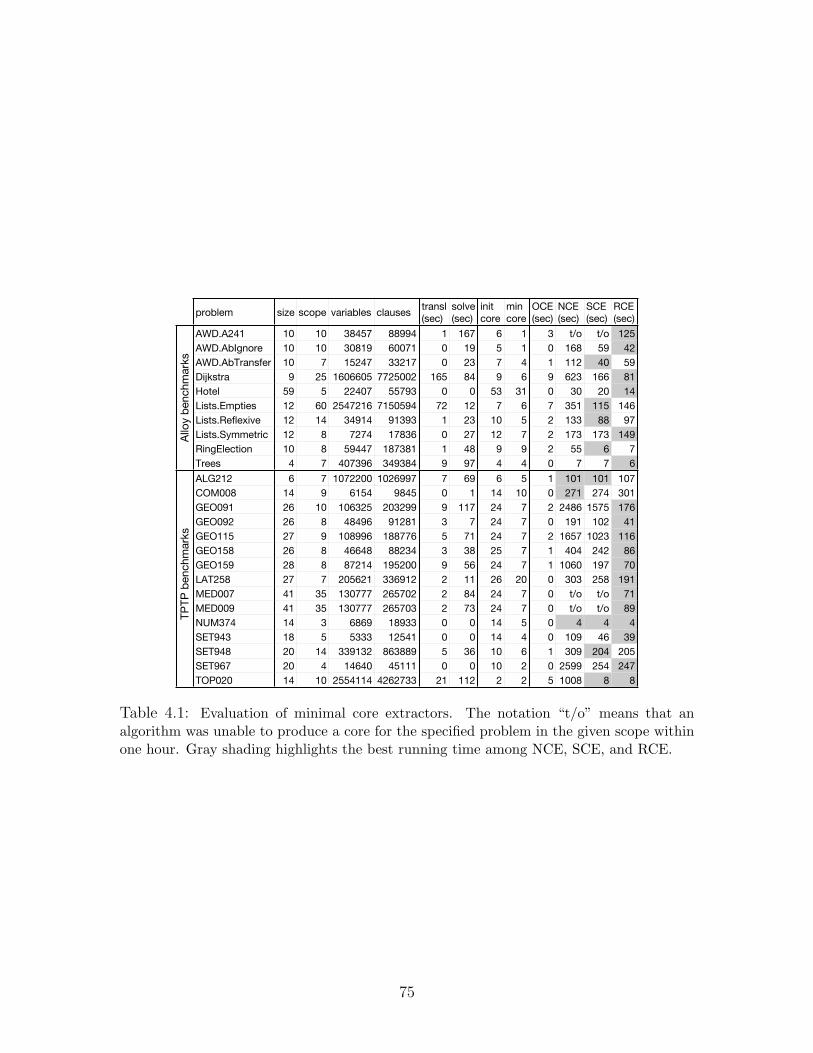
problem size scope variables clausestransl

(sec)

solve

(sec)

init

core

min

core

OCE

(sec)

NCE

(sec)

SCE

(sec)

RCE

(sec)

AWD.A241 10 10 38457 88994 1 167 6 1 3 t/o t/o 125

AWD.AbIgnore 10 10 30819 60071 0 19 5 1 0 168 59 42

AWD.AbTransfer 10 7 15247 33217 0 23 7 4 1 112 40 59

Dijkstra 9 25 1606605 7725002 165 84 9 6 9 623 166 81

Hotel 59 5 22407 55793 0 0 53 31 0 30 20 14

Lists.Empties 12 60 2547216 7150594 72 12 7 6 7 351 115 146

Lists.Reflexive 12 14 34914 91393 1 23 10 5 2 133 88 97

Lists.Symmetric 12 8 7274 17836 0 27 12 7 2 173 173 149

RingElection 10 8 59447 187381 1 48 9 9 2 55 6 7

Trees 4 7 407396 349384 9 97 4 4 0 7 7 6

ALG212 6 7 1072200 1026997 7 69 6 5 1 101 101 107

COM008 14 9 6154 9845 0 1 14 10 0 271 274 301

GEO091 26 10 106325 203299 9 117 24 7 2 2486 1575 176

GEO092 26 8 48496 91281 3 7 24 7 0 191 102 41

GEO115 27 9 108996 188776 5 71 24 7 2 1657 1023 116

GEO158 26 8 46648 88234 3 38 25 7 1 404 242 86

GEO159 28 8 87214 195200 9 56 24 7 1 1060 197 70

LAT258 27 7 205621 336912 2 11 26 20 0 303 258 191

MED007 41 35 130777 265702 2 84 24 7 0 t/o t/o 71

MED009 41 35 130777 265703 2 73 24 7 0 t/o t/o 89

NUM374 14 3 6869 18933 0 0 14 5 0 4 4 4

SET943 18 5 5333 12541 0 0 14 4 0 109 46 39

SET948 20 14 339132 863889 5 36 10 6 1 309 204 205

SET967 20 4 14640 45111 0 0 10 2 0 2599 254 247

TOP020 14 10 2554114 4262733 21 112 2 2 5 1008 8 8

Allo

y b

en

ch

mark

sT

PT

P b

en

ch

mark

s

Table 4.1: Evaluation of minimal core extractors. The notation “t/o” means that analgorithm was unable to produce a core for the specified problem in the given scope withinone hour. Gray shading highlights the best running time among NCE, SCE, and RCE.

75

problem N-scoreNCE /

RCE

average

speed up

NUM374 -0.19 1.07

3.27

SET943 0.12 2.80

SET967 0.21 10.51

Trees 0.58 1.09

COM008 0.60 0.90

Hotel 1.05 2.21

3.21

RingElection 1.72 7.59

ALG212 1.86 0.94

Lists.Empties 1.87 2.40

LAT258 1.88 1.58

Dijkstra 1.94 7.72

AWD.AbTransfer 2.10 1.89

Lists.Symmetric 2.12 1.16

GEO092 2.13 4.68

Lists.Reflexive 2.21 1.37

AWD.AbIgnore 2.24 4.00

SET948 2.70 1.51

GEO158 2.85 4.70

GEO159 3.08 15.06

42.14

TOP020 3.13 131.46

GEO115 3.15 14.34

AWD.A241 3.18 28.81

GEO091 3.35 14.09

MED009 3.40 40.33

MED007 3.45 50.90

easy

med

ium

hard

(a) RCE versus NCE

problem S-scoreSCE /

RCE

average

speed up

NUM374 -0.19 1.08

1.07

SET967 -0.14 1.03

SET943 -0.03 1.19

TOP020 0.35 1.00

Trees 0.58 1.09

COM008 0.60 0.91

RingElection 0.64 0.86

Hotel 0.95 1.44

Lists.Empties 1.11 0.79

AWD.AbTransfer 1.80 0.67

3.63

LAT258 1.81 1.35

ALG212 1.86 0.94

AWD.AbIgnore 1.89 1.40

Dijkstra 1.94 2.06

Lists.Reflexive 2.06 0.91

GEO092 2.08 2.51

Lists.Symmetric 2.12 1.16

SET948 2.16 1.00

GEO158 2.83 2.81

AWD.A241 2.92 28.81

GEO159 2.99 2.80

GEO115 3.08 8.86

27.25MED009 3.13 40.33

MED007 3.13 50.90

GEO091 3.30 8.93

easy

med

ium

hard

(b) RCE versus SCE

Table 4.2: Evaluation of minimal core extractors based on problem difficulty. If an algo-rithm timed out on a given problem (after an hour), its running time for that problem istaken to be one hour.

76

guaranteeing algorithms is given in Table 4.2, where the problems are classified ac-cording to their difficulty for NCE (Table 4.2a) and SCE (Table 4.2b). Tables 4.2and 4.2b show a difficulty rating for each problem; the speed-up of RCE over NCE orSCE on that problem; and the average speed-up of RCE on all problems in a givencategory.

A core extraction problem is rated as easy for NCE if its N-score is less than 1,hard if the score is 3 or more, and moderately hard otherwise. The N-score for aproblem is defined as log10((s−m) ∗ t + m ∗ t ∗ .01), where s is the size of the inputspecification, m is the size of its minimal core, and t is the time, in seconds, taken bythe SAT solver to determine that S is unsatisfiable. The N-score formula predicts howmuch work NCE has to do to eliminate irrelevant constraints from a specification,by predicting that NCE will take (s − m) ∗ t seconds to prune away the (s − m)irrelevant constraints. The formula allocates only 1 percent of the initial solving timeto the testing of a critical constraint because satisfiable formulas are solved quicklyin practice. The difficulty of a problem for SCE is computed in a similar way; theS-score of a given problem is log10((s

′ −m) ∗ t + m ∗ t ∗ .01), where s′ is the size ofthe initial (one-step) core.

Unsurprisingly, OCE outperforms both SCE and RCE in terms of execution time.However, it generates cores that are on average 2.6 times larger than the correspondingminimal cores. For 21 out of the 25 tested problems (84%), the OCE core includedmore than 50% of the original constraints. In contrast, only 8 out of 25 (32%) minimalcores included more than half of the original constraints.

4.4 Related work

The problem of finding unsatisfiable cores has been studied in the context of linearprogramming [23], propositional satisfiability [32, 57, 79, 85, 97, 102, 153], and finitemodel finding [118]. The first half of this section presents an overview of that work.The second half summarizes the work on bounded model checking [52, 120] and otherapplications of SAT [42, 65, 112, 115, 121, 146] that, like RCE, recycle learned clausesfor faster solving of closely related SAT instances.

4.4.1 Minimal core extraction

Among the early work on minimal core extraction is Chinneck and Dravnieks’ [23]deletion filtering algorithm for linear constraints. The algorithm is similar to NCE:given an infeasible linear program LP , it tests each functional constraint for member-ship in an Irreducible Infeasible Subset (i.e. minimal unsatisfiable core) by removingit from LP and applying a linear programming solver to the result. If the reducedLP is infeasible, the constraint is permanently removed, otherwise it is kept. Theremaining algorithms in [23] are specific to linear programs, and there is no obviousway to adapt them to other domains.

Most of the work on extracting small unsatisfiable cores comes from the SATcommunity. Several practical algorithms [57, 102, 153] have been proposed for finding

77

small, but not necessarily minimal, cores of propositional formulas. Zhang and Malik’salgorithm [153], for example, works by extracting a core from a refutation, feeding itback to the solver, and repeating this process until the size of the extracted core nolonger decreases. A few proposed algorithms provide strong optimality guarantees—such as returning the smallest minimal core [85, 97] or all minimal cores [79, 80,59, 61, 60] of a boolean formula—at the cost of scaling to problems that are ordersof magnitude smaller than those handled by the approximation algorithms. TheComplete Resolution Refutation (CRR) algorithm by Dershowitz et al. [32] strikesan attractive balance between scalability and optimality: it finds a single minimalcore but scales to large real-world formulas. CRR was one of the inspirations forRCE and is, in fact, an instantiation of RCE for propositional logic, with a SATsolver as a resolution engine and the identity function as the translation procedure.

The work by Shlyakhter et al. [118] is most closely related to the techniquespresented in this chapter. It proposes one step core extraction (OCE) for declarativespecifications in a language reducible to propositional logic. The algorithm translatesan unsatisfiable specification to propositional logic, obtains an unsatisfiable core ofthe translation from a SAT solver, and returns snippets of the original formula thatcorrespond to the extracted boolean core. Unlike RCE, the OCE method providesno optimality guarantees. In fact, the core it produces is equivalent to the initialcore computed by RCE. As discussed in the previous section, this initial core isrelatively cheap to find, but it tends to be much larger than a minimal core for mostspecifications.

4.4.2 Clause recycling

Many applications of SAT [42, 52, 65, 112, 115, 120, 121, 146] employ techniques forreusing learned clauses to speed up solving of related boolean formulas. Silva andSakallah [121] proposed one of the early clause recycling schemes in the context ofautomatic test pattern generation (ATPG). The ATPG problem involves solving aSAT instance of the form C ∧ F ∧ D, where C is the set of clauses that encodesthe correct behavior of a given circuit, F is the description of a faulty version ofthat circuit, and D states that C and F produce different outputs. A model ofan ATPG formula, known as a test pattern, describes an input to the circuit beingtested that distinguishes between the correct behavior C and the faulty behavior F .Generating test patterns for multiple faults leads to a series of SAT instances of theform C ∧ Fi ∧ Di. Silva and Sakallah’s [121] recycling method is based on reusingconflict clauses3 implied by C, which they call pervasive clauses. This approach doesnot exploit all valid learned clauses, however. If the faulty circuits Fi and Fi+i overlap,clauses learned from Fi ∩ Fi+i are not reused.

Shtrichman [120] generalized the idea of pervasive clauses and applied it in thecontext of SAT-based bounded model checking (BMC) [15, 16]. BMC is the problemof checking if a finite state machine m has a trace of length k or less that violates atemporal property p. Shtrichman’s [120] work focuses on checking properties that hold

3Conflict clauses are resolvents that encode root causes of conflicts detected during search [90].

78

in all states of a given state machine (written as AGp in temporal logic). The checkis performed by applying a SAT solver to the formula I0 ∧Mk ∧Pk, where I0 encodesthe initial state of m, Mk describes all executions of m of length k, and Pk asserts thatp does not hold in at least one of the states described by Mk. A model of the BMCformula represents an execution of m (of length at most k) which violates the propertyp. If there are no counterexamples of length k, the check is repeated for executions oflength k + 1, leading to a series of overlapping SAT instances. Strichman’s methodreuses all conflict clauses that are implied by (I0 ∧Mk ∧ Pk)∩ (I0 ∧Mk+1 ∧ Pk+1). Inthe case of BMC, these are the clauses learned from I0 ∧Mk.

Several clause-recycling techniques have also been proposed in the context of incre-mental SAT solving [42, 65, 146]. Hooker [65] proposed the first incremental techniquefor solving a series of SAT instances of the form C0 ⊆ . . . ⊆ Ck. The technique in-volves reusing all conflict clauses implied by Ci when solving Ci+1. Whittemore et al.[146] extended Hooker’s definition of incremental SAT to allow clause removal. Theirsolver accepts a series of SAT instances C1, . . . , Ck, where each Ci+1 can be obtainedfrom Ci by adding or removing clauses. If clauses are removed from Ci, the solverdiscards all learned clauses that depend on Ci \Ci+1 and reuses the rest. Identifyingthe clauses that need to be discarded is expensive, however, and it requires extrabookkeeping [146] during solving. Een and Sorensson [42] addressed this problemwith an incremental solver that provides limited support for clause removal. In par-ticular, Ci+1 \ Ci can contain any clause, but Ci \ Ci+1 must consist of unit clauses.Since the clauses in Ci \ Ci+1 are treated as decisions by the search procedure, allconflict clauses learned from Ci can be reused when solving Ci+1.

79

80

Chapter 5

Conclusion

Design, implementation, analysis and configuration of software all involve reasoningabout relational structures: organizational hierarchies in the problem domain, ar-chitectural configurations in the high level design, or graphs and linked list in lowlevel code. Until recently, however, engines for solving relational constraints havehad limited applicability. Designed to analyze small, hand-crafted models of softwaresystems, current frameworks perform poorly on large specifications, especially in thepresence of partial models.

This thesis presented a framework for solving large relational problems using SAT.The framework integrates two facilities, a finite model finder and a minimal unsatisfi-able core extractor, accessible through a high-level specification language that extendsrelational logic with a mechanism for specifying partial models (Chapters 1-2). Bothfacilities are based on new techniques. The model finder uses a new translation toSAT (Chapter 2) and a new algorithm for detecting symmetries in the presence ofpartial models (Chapter 3), while the core extractor uses a new method for recyclinginferences made at the boolean level to speed up core minimization at the specificationlevel (Chapter 4).

The work presented here has been prototyped and evaluated in Kodkod, a new rela-tional engine with recent applications to declarative configuration [101, 149], test-casegeneration [114, 135] and bounded verification [21, 31, 34, 126, 137]. The adoption anduse of Kodkod by the wider community has highlighted both strengths and limitationsof its techniques. The former include efficiency on specifications with partial models,low-arity relations and rich type hierarchies; the latter include limited scalability inthe presence of high-arity relations, transitive closure and deeply nested quantifiers.This chapter concludes the thesis with a summary of the key contributions behindKodkod, a discussion of the tool’s applicability compared to other solvers, and anoutline of directions for future work.

5.1 Discussion

The key contributions of this work are a new relational language that supports partialmodels; a new translation from relational logic to SAT that uses sparse matrices and

81

Kod

kod

IDP1.

3[8

8]Par

adox

2.3

[25]

Dar

win

FM

[13]

Mac

e4[9

2]

languagefirst order logicrelational algebrapartial modelsinductive definitionstypesbitvector arithmetic

model findingpartial modelsinductive definitionssymmetry breakinghigh-arity relationsnested quantifiers

core extractionminimal core

Table 5.1: Features of state-of-the-art model finders. Filled diamonds indicate that aspecified feature is fully supported by a solver; half-filled diamonds indicate limited support;and empty diamonds indicate no support.

auto-compacting circuits; a new algorithm for detecting symmetries in the presence ofpartial models; and a new algorithm for finding minimal cores with resolution-basedengines. The language and the techniques combine into a framework that is well-suited to solving problems in both declarative configuration and analysis. Kodkod iscurrently the only engine (Table 5.1) that scales both in the presence of symmetries(which is crucial for declarative analysis) and partial models (which is crucial fordeclarative configuration). It is also the only model finding engine that incorporatesa facility for the extraction of minimal cores.

This thesis focused on efficient analysis of specifications that commonly arise indeclarative configuration and bounded verification. Such specifications are charac-terized by the use of typed relations with low arity, set-theoretic operators and join,shallowly nested (universal) quantifiers, and state spaces with partial models or manysymmetries. Kodkod outperforms existing tools significantly on specifications withthese features (e.g. the Sudoku examples from Chapter 1). It is, however, less effectivethan some of the existing solvers on other classes of problems.

DarwinFM [13], for example, is the most efficient model finder for specificationscomprised of first order clauses over high-arity relations. It works by translating

82

a formula in unsorted first order logic to a set of function-free first order clauses,which are solved using the Darwin [14] decision procedure. A key advantage of thisapproach over SAT-based approaches is its space efficiency. In particular, the size ofpropositional encodings for first order or relational formulas grows exponentially withuniverse size and relation arity. The size of Darwin encodings, on the other hand, islinear in universe size. As a result, DarwinFM can handle formulas with high-arityrelations (e.g. arity 56) on which other model finders run out of resources [125].

IDP1.3 [88] is, like Kodkod, a model extender. Unlike Kodkod, however, it targetsspecifications in sorted first order logic with inductive definitions (FOL/ID). Givena specification in FOL/ID, the tool translates it to a set of clauses in propositionallogic with inductive definitions. These clauses are then tested for satisfiability usingMiniSatID [89]. Because its underlying engine supports inductive definitions, IDP1.3performs much better in their presence than Kodkod. It can, for example, find aHamiltonian cycle in a graph with 200 nodes and 1800 edges in less than a second[147]. Kodkod, in contrast, scales only to graphs with about 30 nodes and 100 edges.

Paradox2.3 [25] is a traditional SAT-based model finder for unsorted first orderlogic. Unlike other SAT-based tools, Paradox2.3 searches for models incrementally.In particular, it translates the input formula to SAT in a universe of size k and feedsthe result to an instance of MiniSat [43]. If the solver finds a model, it is translatedto a model of the original specification and the search terminates. Otherwise, theclauses specific to the universe size are retracted from the solver’s database, followedby the addition of new clauses that turn the solver’s database into a valid translationof the original specification in a universe of size k + 1. This enables the SAT solverto reuse search information between consecutive universe sizes, making the tool well-suited to analyses whose goal is to find a model in some universe rather than test aspecification’s satisfiability in a specific universe. Paradox2.3 also employs a numberof heuristics [25] that enable it to translate specifications in unsorted FOL much moreefficiently than Kodkod, especially in the presence of deeply nested quantifiers.

Mace4 [92] implements a dedicated search algorithm for finding models of specifi-cations in unsorted first order logic. Its search engine performs on-the-fly symmetrybreaking using a variant of the Least Number Heuristic [151]. Search combined withdynamic symmetry breaking is particularly effective on specifications that arise ingroup theory. Such specifications have highly symmetric state spaces and consistof formulas that compare deeply nested terms for equality. Predecessors of Mace4[51, 151, 152] have all been used to solve open problems in abstract algebra, andsearch-based tools remain the most efficient model finders for this class of problems.

5.2 Future work

The techniques presented here have significantly extended the scalability and appli-cability of relational model finding. Kodkod is orders of magnitude faster than priorrelational engines [68, 70, 117] and includes a unique combination of features thatmake it suitable for both declarative configuration [101, 149] and analysis [21, 31, 34,114, 126, 135, 137]. But a number of scalability and usability problems still remain.

83

The engine currently implements only rudimentary techniques for deciding bitvectorarithmetic; its support for inductive definitions is very limited; it includes no specialhandling for simpler fragments of its input language; and it does not incorporate anyheuristics for choosing good variable and constraint orderings either in the context ofmodel finding or core extraction.

5.2.1 Bitvector arithmetic and inductive definitions

The need for better handling of arithmetic and inductive definitions arose in severalapplications [21, 31, 149] of Kodkod. At the moment, the tool handles both arithmeticand transitive closure by direct translation to SAT. This approach, known as “bit-blasting,” is effective for some problems. For example, Kodkod is as efficient asstate-of-the-art SMT solvers on specifications in which bitvectors are combined withlow-level operators (shifts, ands, and ors) and compared for (in)equality [46]. Ingeneral, however, bit-blasting yields large and hard to solve boolean formulas.

An interesting direction for future work would be to explore if bit-blasting can beavoided, or at least minimized, with the aid of two recently developed SMT techniques[53, 89]. The first [53] is a linear solver for eliminating redundant variables frombitvector expressions prior to bit-blasting; the second [89] is a new SAT solver thatsupports inductive definitions. The former would have to be adapted for use withKodkod because most bitvector variables that appear in Kodkod formulas are notfree: they represent cardinalities of relations or sums of integer-valued atoms in a set.Exploiting the latter would require extending CBCs (Chapter 2) with a new circuitthat represents definitional implication [89] and changing the translation procedureto take advantage of this circuit.

5.2.2 Special-purpose translation for logic fragments

Because sets and scalars are treated as relations in bounded relational logic, Kodkod’stranslator represents every expression as a matrix of boolean values. Operationson expressions are translated using matrix operations: join corresponds to matrixmultiplication, union to disjunction, intersection to conjunction, etc. The resultingtranslation algorithm is effective on specifications that make heavy use of relationaloperators. It is, however, much less efficient than the translators employed in Para-dox2.3 and IDP1.3 on specifications that are essentially fragments of first order logic.

In particular, given a specification in which the only operations on relations arefunction application and membership testing, Kodkod’s translator expends a largeamount of resources on creating matrices and multiplying them when all that is neededto translate such a specification is a series of table lookups. This overhead is negligiblefor small and medium-sized problems. But for large problems with nested quantifiers,it makes a difference between generating a translation in a few seconds and severalminutes. For example, Kodkod takes nearly 3 minutes to translate a specificationthat says a graph [147] with 7,260 vertices and 21,420 edges is 3-colorable. IDP1.3, incontrast, translates the same specification in less than a second. Similar performance

84

can be elicited from Kodkod only if the specification is re-written so that all joins areeliminated.

An important direction for future work is the development of special-purposetranslation techniques for inputs that are specified in simpler fragments of Kodkod’sinput language. This would require solving two problems: identifying specifications(or parts thereof) that are eligible for faster translation, and translating the identifiedfragments in a more efficient manner. The latter could be accomplished either byadapting the techniques used in other solvers or by incorporating those solvers intoKodkod. The hybrid approach seems particularly appealing, since Kodkod’s userswould benefit automatically from any improvements to the underlying solvers, justas they automatically benefit from improvements in the SAT technology.

5.2.3 Heuristics for variable and constraint ordering

It is well-known that SAT solvers are sensitive to the order in which variables andclauses are presented to them, with small perturbations in input ordering causinglarge differences in runtime. MiniSat, for example, can take anywhere between 1.5and 5 minutes to solve the problem AWD.A241 from Chapter 2, depending on theorder in which its constraints are translated. Similarly, the order in which constraintsare selected for pruning during core extraction (Chapter 4) often make the differencebetween finding a minimal core in a few seconds and giving up after a few hours.

The problem of choosing a good (variable) ordering has been studied extensivelyin the SAT community [3, 4, 5, 17, 35, 37, 36, 66, 98]. Heuristics that work at theboolean level, however, do not take into account domain-level knowledge. Recent workon choosing variable orderings for specific problems, such as graph coloring [140] orbounded model checking [142], has shown that heuristics based on domain knowledgecan significantly outperform more generic approaches. Corresponding heuristics havenot yet been developed for SAT-based model finding. The same is true for core extrac-tion; no heuristics have been developed for choosing a good minimization order for agiven core. Both of these are exciting and promising areas for future research, witha potential to further extend the efficiency and applicability of declarative problemsolving.

85

86

Bibliography

[1] Parosh Aziz Abdulla, Per Bjesse, and Niklas Een. Symbolic reachability anal-ysis based on sat-solvers. In TACAS ’00, pages 411–425, London, UK, 2000.Springer-Verlag.

[2] Jean-Raymond Abrial. The B-Book: Assigning Programs to Meanings. Cam-bridge University Press, 1996.

[3] Fadi A. Aloul, Igor L. Markov, and Karem A. Sakallah. Mince: a static globalvariable-ordering for SAT and BDD. In Proc. Int’l Workshop on Logic andSynthesis, University of Michigan, June 2001.

[4] Fadi A. Aloul, Igor L. Markov, and Karem A. Sakallah. FORCE: a fast andeasy-to-implement variable-ordering heuristic. In GLSVLSI ’03: Proceedingsof the 13th ACM Great Lakes symposium on VLSI, pages 116–119, New York,NY, USA, 2003. ACM.

[5] E. Amir and S. McIlraith. Solving satisfiability using decomposition and themost constrained subproblem. In SAT’01, 2001.

[6] Henrik Reif Andersen and Henrik Hulgaard. Boolean expression diagrams. InLICS ’97, Warsaw, Poland, June 1997.

[7] M. A. Armstrong. Groups and Symmetry. Springer-Verlag, New York, 1988.

[8] L. Babai, W. M. Kantor, and E. M. Luks. Computational complexity and theclassification of finite simple groups. In IEEE SFCS, pages 162–171. IEEE CSP,1983.

[9] Domagoj Babic and Frank Hutter. Spear. In SAT 2007 Competition, 2007.

[10] R. Backofen and S. Will. Excluding symmetries in concurrent constraint pro-gramming. In Workshop on Modeling and Computing with Concurrent Con-straint Programming, 1998.

[11] R. Backofen and S. Will. Excluding symmetries in constraint-based search.In Proc. Principles and Practice of Constraint Programming (CP’99), volumeLNCS 1713, pages 73–87. Springer, 1999.

87

[12] R. Barrett, M. Berry, T. F. Chan, J. Demmel, J. Donato, J. Dongarra, V. Ei-jkhout, R. Pozo, C. Romine, and H. Van der Vorst. Templates for the Solutionof Linear Systems: Building Blocks for Iterative Methods. SIAM, Philadelphia,PA, 2nd edition, 1994.

[13] Peter Baumgartner, Alexander Fuchs, Hans de Nivelle, and Cesare Tinelli.Computing finite models by reduction to function-free clause logic. Journalof Applied Logic, 2007.

[14] Peter Baumgartner, Alexander Fuchs, and Cesare Tinelli. Implementing themodel evolution calculus. International Journal of Artificial Intelligence Tools,15(1):21–52, 2006.

[15] Armin Biere, Alessandro Cimatti, Edmund M. Clarke, Ofer Shtrichman, andYunshan Zhu. Bounded model checking. Advances in Computers, 58, 2003.

[16] Armin Biere, Alessandro Cimatti, Edmund M. Clarke, and Yunshan Zhu. Sym-bolic model checking without BDDs. In TACAS’99: Proc. of the 5th Int’l Conf.on Tools and Algorithms for Construction and Analysis of Systems, pages 193–207, London, UK, 1999. Springer-Verlag.

[17] P. Bjesse, J. Kukula, R. Damiano, T. Stanion, and Y. Zhu. Guiding SATdiagnosis with tree decompositions. In SAT ’03, 2003.

[18] Per Bjesse and Arne Boralv. DAG-aware circuit compression for formal ver-ification. In Proc. 2004 IEEE/ACM Int’l Conf. on Computer-Aided Design(ICCAD’04), pages 42–49, Washington, DC, USA, 2004. IEEE Computer So-ciety.

[19] Robert Brummayer and Armin Biere. Local two-level and-inverter graph min-imization without blowup. In Proc. 2nd Doctoral Workshop on Mathematicaland Engineering Methods in Computer Science (MEMICS ’06), October 2006.

[20] E. J. H. Chang and R. Roberts. An improved algorithm for decentral-ized extrema-finding in circular configurations of processes. Commun. ACM,22(5):281–283, 1979.

[21] Felix Chang. Alloy analyzer 4.0. http://alloy.mit.edu/alloy4/, 2007.

[22] Peter Pin-Shan Chen. The entity-relationship model—toward a unified view ofdata. ACM Trans. Database Syst., 1(1):9–36, 1976.

[23] John W. Chinneck and Erik W. Dravnieks. Locating minimal infeasible con-straint sets in linear programs. ORSA Journal of Computing, 3(2):157–158,1991.

[24] M. Cierniak and W. Li. Unifying data and control transformations fordistributed shared memory machines. Technical Report TR-542, Univ. ofRochester, November 1994.

88

[25] Koen Claessen and Niklas Sorensson. New techniques that improve MACE-stylefinite model finding. In CADE-19 Workshop on Model Computation, Miami,FL, July 2003.

[26] David Cohen, Peter Jeavons, Christopher Jefferson, Karen E. Petrie, and Bar-bara Smith. Symmetry definitions for constraint satisfaction problems. In Proc.Principles and Practice of Constraint Programming (CP’05), volume LNCS3709, pages 17–31. Springer Berlin, 2005.

[27] James Crawford, Matthew L. Ginsberg, Eugene Luck, and Amitabha Roy.Symmetry-breaking predicates for search problems. In KR’96, pages 148–159.Morgan Kaufmann, San Francisco, 1996.

[28] Paul T. Darga, Karem A. Sakallah, and Igor L. Markov. Faster symmetrydiscovery using sparsity of symmetries. In Proc. 45th Design Automation Con-ference, Anaheim, California, June 2008.

[29] Leonardo de Moura and Nikolaj Bjørner. Z3: An efficient SMT solver. InTACAS’08, Budapest, Hungary, 2008.

[30] Greg Dennis, Kuat Yessenov, and Daniel Jackson. Bounded verification ofvoting software. In VSTTE’08, Toronto, Canada, October 2008.

[31] Gregory Dennis, Felix Chang, and Daniel Jackson. Modular verification of code.In ISSTA ’06, Portland, Maine, July 2006.

[32] Nachum Dershowitz, Ziyad Hanna, and Alexander Nadel. A scalable algorithmfor minimal unsatisfiable core extraction. In SAT ’06, LNCS, pages 36–41.Springer Berlin, 2006.

[33] E. W. Dijkstra. Cooperating sequential processes. In F. Genuys, editor, Pro-gramming Languages, pages 43–112. Academic Press, New York, 1968.

[34] Julian Dolby, Mandana Vaziri, and Frank Tip. Finding bugs efficiently with asat solver. In ESEC-FSE ’07, pages 195–204, New York, NY, USA, 2007. ACM.

[35] V. Durairaj and P. Kalla. Guiding cnf-sat search via efficient constraint par-titioning. In ICCAD ’04: Proceedings of the 2004 IEEE/ACM Internationalconference on Computer-aided design, pages 498–501, Washington, DC, USA,2004. IEEE Computer Society.

[36] Vijay Durairaj and Priyank Kalla. Variable ordering for efficient SAT searchby analyzing constraint-variable dependencies. In SAT ’05, pages 415–422.Springer, 2005.

[37] Vijay Durairaj and Priyank Kalla. Guiding CNF-SAT search by analyzingconstraint-variable dependencies and clause lengths. High-Level Design Vali-dation and Test Workshop, 2006. Eleventh Annual IEEE International, pages155–161, Nov. 2006.

89

[38] Bruno Dutertre and Leonardo de Moura. A fast linear-arithmetic solver forDPLL(T). In CAV’06, LNCS, pages 81–94. Springer-Verlag, 2006.

[39] Jonathan Edwards, Daniel Jackson, and Emina Torlak. A type system forobject models. In SIGSOFT ’04/FSE-12, pages 189–199, New York, NY, USA,2004. ACM Press.

[40] Jonathan Edwards, Daniel Jackson, Emina Torlak, and Vincent Yeung. Fasterconstraint solving with subtypes. In ISSTA ’04, pages 232–242, New York, NY,USA, 2004. ACM Press.

[41] Niklas Een and Armin Biere. Effective preprocessing in SAT through variableand clause elimination. In SAT ’05, 2005.

[42] Niklas Een and Niklas Sorensson. Temporal induction by incremental SAT solv-ing. In Proc. of the 1st Int’l Workshop on Bounded Model Checking (BMC’03),Boulder, Colorado, July 2003.

[43] Niklas Een and Niklas Sorensson. An extensible SAT-solver. In SAT’03, volumeLNCS 2919, pages 502–518, 2004.

[44] Niklas Een and Niklas Sorensson. Translating pseudo-boolean constraints intoSAT. In SBMC, volume 2, pages 1–26, 2006.

[45] T. Fahle, S. Schamberger, and M. Sellmann. Symmetry breaking. In Proc.Principles and Practice of Constraint Programming (CP’01), volume LNCS2239, pages 93–107. Springer, 2001.

[46] Mendy Fisch. Using satisfiability solvers to test network configuration, October2008.

[47] P. Flener, A. Frisch, B. Hnich, Z. Kiziltan, I. Miguel, J. Pearson, and T. Walsh.Breaking row and column symmetries in matrix models. In P. van Hentenryck,editor, Proc. Principles and Practice of Constraint Programming (CP’02), vol-ume LNCS 2470, pages 462–476. Springer-Verlag, 2002.

[48] F. Focacci and M. Milano. Global cut framework for removing symmetries.In Proc. Principles and Practice of Constraint Programming (CP’01), volumeLNCS 2239, pages 72–92. Springer, 2001.

[49] Formal Methods Group at ITC-IRST, Model Checking Group at CMU, Mech-anized Reasoning Group at U. of Genova, and Mechanized Reasoning Group atU. of Trento. NuSMV: a new symbolic model checker. http://nusmv.irst.itc.it/,August 2008.

[50] A. M. Frisch, C. Jefferson, and I. Miguel. Symmetry breaking as a preludeto implied constraints: a constraint modelling pattern. IJCAI, pages 109–116,2005.

90

[51] Masayuki Fujita, John Slaney, and Frank Bennett. Automating generation ofsome results in finite algebra. In 13th IJCAI, Chambery, France, 1993.

[52] Malay K. Ganai, Aarti Gupta, and Pranav Ashar. Beyond safety: customizedSAT-based model checking. In DAC’05: Proc. of the 42nd Conf. on DesignAutomation, pages 738–743, New York, NY, USA, 2005. ACM.

[53] Vijay Ganesh. Decision Procedures for Bit-Vectors, Arrays and Integers. PhDthesis, Stanford University, Stanford, CA, September 2007.

[54] Ian P. Gent and Iain McDonald. NuSBDS: Symmetry breaking made easy.In Barbara Smith, Ian P. Gent, and Warwick Harvey, editors, Proc. 3rd Int’lWorkshop on Symmetry in CSPs, pages 153–160, 2003.

[55] Ian P. Gent, Karen E. Petrie, and Jean-Francois Puget. Symmetry in constraintprogramming. In F. Rossi, P. van Beek, and T. Walsh, editors, Handbook ofConstraint Programming, chapter 10. Elsevier Science Publishers B. V., 2006.

[56] E. Goldberg and Y. Novikov. BerkMin: A fast and robust SAT solver. In DATE’02, pages 142–149, 2002.

[57] Evgueni Goldberg and Yakov Novikov. Verification of proofs of unsatisfiabilityfor CNF formulas. In DATE ’03, 2003.

[58] Peter Green. 200 Difficult Sudoku Puzzles. Lulu Press, 2nd edition, July 2005.

[59] Eric Gregoire, Bertrand Mazure, and Cedric Piette. Extracting MUSes. InECAI’06, pages 387–391, Trento (Italy), August 2006.

[60] Eric Gregoire, Bertrand Mazure, and Cedric Piette. Boosting a complete tech-nique to find MSS and MUS thanks to a local search oracle. In IJCAI’07,volume 2, pages 2300–2305, Hyderabad (India), January 2007.

[61] Eric Gregoire, Bertrand Mazure, and Cedric Piette. Local-search extraction ofMUSes. Constraints Journal, 12(3):324–344, 2007.

[62] Michael Hammer and Dennis McLeod. The semantic data model: a modellingmechanism for data base applications. In SIGMOD’78: Proceedings of the 1978ACM SIGMOD Int’l Conf. on Management of Data, pages 26–36, New York,NY, USA, 1978. ACM.

[63] Vegard Hanssen. Sudoku puzzles. http://www.menneske.no/sudoku/eng/, July2008.

[64] Warwick Harvey, Tom Kelsey, and Karen Petrie. Symmetry group expressionsfor CSPs. In Barbara Smith, Ian P. Gent, and Warwick Harvey, editors, Proc.3rd Int’l Workshop on Symmetry in CSPs, pages 86–96, 2003.

[65] J. N. Hooker. Solving the incremental satisfiability problem. J. Log. Program.,15(1-2):177–186, 1993.

91

[66] J. Huang and A. Darwiche. A structure-based variable ordering heuristic forSAT. In Proc. 1st Int’l Joint Conference on Artificial Intelligence (IJCAI),pages 1167–1172, August 2003.

[67] Daniel Jackson. An intermediate design language and its analysis. In FSE’98,November 1998.

[68] Daniel Jackson. Automating first order relational logic. In FSE ’00, San Diego,CA, November 2000.

[69] Daniel Jackson. Software Abstractions: logic, language, and analysis. MITPress, Cambridge, MA, 2006.

[70] Daniel Jackson, Somesh Jha, and Craig A. Damon. Isomorph-free model enu-meration: a new method for checking relational specifications. ACM TPLS,20(2):302–343, March 1998.

[71] Daniel Jackson, Ilya Shlyakhter, and Manu Sridharan. A micromodularitymechanism. In ESEC / SIGSOFT FSE ’01, pages 62–73, 2001.

[72] Tommi Junttila and Petteri Kaski. Engineering an efficient canonical labelingtool for large and sparse graphs. In ALENEX 2007, New Orleans, Lousiana,January 2007.

[73] T. Jussila and Armin Biere. Compressing BMC encodings with QBF. In Proc.BMC’06, 2006.

[74] John A. Kalman. Automated Reasoning with Otter. Rinton Press, 2001.

[75] Eunsuk Kang and Daniel Jackson. Formal modeling and analysis of a flashfilesystem in Alloy. In ABZ’08, London, UK, September 2008.

[76] Sarfraz Khurshid. Generating Structurally Complex Tests from Declarative Con-straints. PhD thesis, Massachusetts Institute of Technology, February 2003.

[77] Sarfraz Khurshid and Darko Marinov. TestEra: Specification-based testing ofjava programs using sat. ASE ’00, 11(4):403–434, 2004.

[78] Andreas Kuehlmann, Viresh Paruthi, Florian Krohm, and Malay K. Ganai.Robust boolean reasoning for equivalence checking and functional property ver-ification. IEEE Transactions on CAD, 21(12):1377–1394, December 2002.

[79] Mark H. Liffiton and Karem A. Sakallah. On finding all minimally unsatisfiablesubformulas. In SAT ’05, 2005.

[80] Mark H. Liffiton and Karem A. Sakallah. Algorithms for computing minimalunsatisfiable subsets of constraints. Journal of Automated Reasoning, 40(1):1–33, January 2008.

92

[81] Amerson Lin, Mike Bond, and Joylon Clulow. Modeling partial attacks withAlloy. In Security Protocols Workshop (SPW’07), Brno, Czech republic, April2007.

[82] Chun-Yuan Lin, Yeh-Ching Chung, and Jen-Shiu Liu. Efficient data compres-sion methods for multidimensional sparse array operations. In Proc. 1st Int’lSymp. on Cyber Worlds (CW’02), Tokyo, Japan, 2002.

[83] Chun-Yuan Lin, Jen-Shiu Liu, and Yeh-Ching Chung. Efficient representationscheme for multidimensional array operations. IEEE Transactions on Comput-ers, 51(3), March 2002.

[84] Mikel Lujan, Anila Usman, Patrick Hardie, T.L. Friedman, and John R. Gurd.Storage formats for sparse matrices in Java. In ICCS 2005, number 3514 inLNCS, pages 365–371, 2005.

[85] Ines Lynce and Jo ao Marques-Silva. On computing minimum unsatisfiablecores. In SAT ’04, 2004.

[86] Ines Lynce and Joel Ouaknine. Sudoku as a SAT problem. In 9th Int. Symp.on AI and Mathematics, January 2006.

[87] Yogesh S. Mahajan, Zhaohui Fu, and Sharad Malik. zchaff2004: An efficientSAT solver. In SAT (Selected Papers), pages 360–375, 2004.

[88] Maarten Marien, Johan Wittocx, and Marc Denecker. The IDP framework fordeclarative problem solving. In E. Giunchiglia, V. Marek, D. Mitchell, andE. Ternovska, editors, Search and Logic: Answer Set Programming and SAT,pages 19–34, 2006.

[89] Maarten Marien, Johan Wittocx, Marc Denecker, and Maurice Bruynooghe.SAT(ID): Satisfiability for propositional logic with inductive definitions. InHans Kleine Buning and Xishun Zhao, editors, SAT, volume 4996 of LCNS,pages 211–224. Springer, 2008.

[90] J. P. Marques-Silva and K. A. Sakallah. GRASP: a search algorithm for propo-sitional satisfiability. Transactions on Computers, 48(5):506–521, 1999.

[91] William McCune. A Davis-Putnam program and its application to finite first-order model search: quasigroup existence problem. Technical report, ANL,1994.

[92] William McCune. Mace4 reference manual and guide. Technical Memorandum264, Argonne National Laboratory, August 2003.

[93] William McCune. Prover9 and MACE4.http://www.cs.unm.edu/ mccune/prover9/, June 2008.

93

[94] Brendan D. McKay. Practical graph isomorphism. Congress Numerantium,30:45–87, 1981.

[95] Kenneth L. McMillan. Symbolic Model Checking. Kluwer Academic Publishers,Norwell, MA, 1993.

[96] David Mitchell and Eugenia Ternovska. A framework for representing and solv-ing np search problems. In AAAI’05, pages 430–435. AAAI Press / MIT Press,2005.

[97] Maher Mneimneh, Ines Lynce, Zaher Andraus, Jo ao Marques-Silva, andKarem A. Sakallah. A branch and bound algorithm for extracting smallestminimal unsatisfiable formulas. In SAT ’05, 2005.

[98] M. Moskewicz, C. F. Madigan, Y. Zhao, L. Zhang, and S. Malik. Chaff: engi-neering an efficient sat solver. In DAC’01, pages 530–535, 2001.

[99] Sanjai Narain. Network configuration management via model finding. In ACMWorkshop On Self-Managed Systems, Newport Beach, CA, October 2004.

[100] Sanjai Narain. ConfigAssure. http://www.research.telcordia.com/bios/narain/,December 2007.

[101] Sanjai Narain, Gary Levin, Vikram Kaul, and Sharad Malik. Declarative infras-tructure configuration synthesis and debugging. Journal of Network Systemsand Management, Special Issue on Security Configuration, 2008.

[102] Yoonna Oh, Maher Mneimneh, Zaher Andraus, Karem Sakallah, and IgorMarkov. Amuse: A minimally-unsatisfiable subformula extractor. In DAC,pages 518–523. ACM/IEEE, June 2004.

[103] J. F. Puget. Symmetry breaking using stabilizers. In F. Rossi, editor, Proc.Principles and Practice of Constraint Programming (CP’03), volume LNCS2833, pages 585–599. Springer, 2003.

[104] J. F. Puget. Breaking symmetries in all-different problems. IJCAI, pages 272–277, 2005.

[105] Jean-Francois Puget. Automatic detection of variable and value symmetries. InP. van Beek, editor, Proc. Principles and Practice of Constraint Programming(CP’05), volume LNCS 3709, pages 475–489. Springer-Verlag, 2005.

[106] Tahina Ramananandro. The Mondex case study with Alloy.http://www.eleves.ens.fr/home/ramanana/work/mondex/, 2006.

[107] Arathi Ramani and Igor L. Markov. Automatically exploiting symmetries inconstraint programming. In B. Faltings et al., editor, Proc. CSCLP’04, volumeLNAI 3419, pages 98–112. Springer-Verlag, 2005.

94

[108] A. Riazanov. Implementing an Efficient Theorem Prover. PhD Thesis, TheUniversity of Manchester, Manchester, July 2003.

[109] J. A. Robinson. A machine-oriented logic based on the resolution principle. J.ACM, 12(1):23–41, 1965.

[110] Gordon Royle. Minimum sudoku. http://people.csse.uwa.edu.au/gordon/sudokumin.php,July 2008.

[111] Ashish Sabharwal. SymChaff: A structure-aware satisfiability solver. In AAAI’05, pages 467–474, Pittsburgh, PA, July 2005.

[112] Sean Safarpour, Andreas Veneris, Gregg Baeckler, and Richard Yuan. EfficientSAT-based boolean matching for FPGA technology mapping. In DAC’06: Proc.of the 43rd Conf. on Design Automation, pages 466–471, New York, NY, USA,2006. ACM.

[113] Robert Seater, Daniel Jackson, and Rohit Gheyi. Requirement progressionin problem frames: deriving specifications from requirements. RequirementsEngineering Journal (REJ’07), 2007.

[114] Danhua Shao, Sarfraz Khurshid, and Dewayne Perry. Whispec: White-box test-ing of libraries using declarative specifications. In LCSD’07, Montreal, October2007.

[115] ShengYu Shen, Ying Qin, and SiKun Li. Minimizing counterexample with unitcore extraction and SAT. In VMCAI’05, Paris, France, January 2005.

[116] Ilya Shlyakhter. Generating effective symmetry breaking predicates for searchproblems. Electronic Notes in Discrete Mathematics, 9, June 2001.

[117] Ilya Shlyakhter. Declarative Symbolic Pure Logic Model Checking. PhD thesis,Massachusetts Institute of Technology, Cambridge, MA, February 2005.

[118] Ilya Shlyakhter, Robert Seater, Daniel Jackson, Manu Sridharan, and ManaTaghdiri. Debugging overconstrained declarative models using unsatisfiablecores. In ASE ’03, 2003.

[119] Ilya Shlyakhter, Manu Sridharan, Robert Seater, and Daniel Jackson. Exploit-ing subformula sharing in automatic analysis of quantified formulas. In SAT’03, Portofino, Italy, May 2003.

[120] Ofer Shtrichman. Pruning techniques for the SAT-based bounded model check-ing problem. In CHARME’01: Proc. of the 11th IFIP WG 10.5 Advanced Re-search Working Conf. on Correct Hardware Design and Verification Methods,pages 58–70, London, UK, 2001. Springer-Verlag.

95

[121] Joao P. Marques Silva and Karem A. Sakallah. Robust search algorithms for testpattern generation. In FTCS’97: Proc. of the 27th Int’l Symposium on Fault-Tolerant Computing, page 152, Washington, DC, USA, 1997. IEEE ComputerSociety.

[122] John K. Slaney. Finder: Finite domain enumerator - system description. InCADE-12, pages 798–801, London, UK, 1994. Springer-Verlag.

[123] J. Michael Spivey. The Z Notation: A Reference Manual. International Seriesin Computer Science. Prentice Hall, 1992.

[124] G. Sutcliffe and C.B. Suttner. The TPTP Problem Library: CNF Releasev1.2.1. Journal of Automated Reasoning, 21(2):177–203, 1998.

[125] Geoff Sutcliffe. The CADE ATP system competition.http://www.cs.miami.edu/ tptp/CASC/J4/, October 2008.

[126] Mana Taghdiri. Automating Modular Program Verification by Refining Specifi-cations. PhD thesis, Massachusetts Institute of Technology, 2007.

[127] Alfred Tarski. On the calculus of relations. Journal of Symbolic Logic, 6:73–89,1941.

[128] Emina Torlak. Subtyping in alloy. Master’s thesis, MIT, May 2004.

[129] Emina Torlak, Felix Chang, and Daniel Jackson. Finding minimal unsatisfiablecores of declarative specifications. In FM ’08, May 2008.

[130] Emina Torlak and Greg Dennis. Kodkod for Alloy users. In First ACM AlloyWorkshop, Portland, Oregon, November 2006.

[131] Emina Torlak and Daniel Jackson. Kodkod: A relational model finder. InTACAS ’07, Braga, Portugal, 2007.

[132] Michael Trick. Graph coloring instances.http://mat.gsia.cmu.edu/COLOR/instances.html, October 2008.

[133] Chris Tucker, David Schuffelton, Ranjitt Jhala, and Sorin Lerner. OPIUM:Optimizing package install/uninstall manager. In Proc. 29th Int. Conf. in Soft.Eng. (ICSE’07), Minneapolis, Minnesota, May 2007.

[134] Engin Uzuncaova, Daniel Garcia, Sarfraz Khurshid, and Don Batory. Aspecification-based approach to testing software product lines. In ESEC-FSE’07, pages 525–528, New York, NY, USA, 2007. ACM.

[135] Engin Uzuncaova, Daniel Garcia, Sarfraz Khurshid, and Don Batory. Testingsoftware product lines using incremental test generation. In ISSRE’08, Seattle/ Redmond, WA, November 2008.

96

[136] Engin Uzuncaova and Sarfraz Khurshid. Kato: A program slicing tool fordeclarative specifications. In ICSE’07, pages 767–770, Washington, DC, USA,2007. IEEE Computer Society.

[137] Engin Uzuncaova and Sarfraz Khurshid. Constraint prioritization for efficientanalysis of declarative models. In FM ’08, Turku, Finland, 2008.

[138] Mandana Vaziri. Finding Bugs in Software with a Constraint Solver. PhDthesis, Massachusetts Institute of Technology, Cambridge, MA, February 2004.

[139] Miroslav N. Velev. Efficient translation of boolean formulas to CNF in formalverification of microprocessors. In ASP-DAC ’04, pages 310–315, January 2004.

[140] Miroslav N. Velev. Exploiting hierarchy and structure to efficiently solve graphcoloring as sat. In ICCAD ’07: Proceedings of the 2007 IEEE/ACM interna-tional conference on Computer-aided design, pages 135–142, Piscataway, NJ,USA, 2007. IEEE Press.

[141] Pete Wake. Sudoku solver by logic. http://www.sudokusolver.co.uk/, Septem-ber 2005.

[142] Chao Wang, HoonSang Jin, Gary D. Hachtel, and Fabio Somenzi. Refining theSAT decision ordering for bounded model checking. In DAC ’04: Proceedingsof the 41st annual conference on Design automation, pages 535–538, New York,NY, USA, 2004. ACM.

[143] Jos Warmer and Anneke Kelppe. The Object Constraint Language: PreciseModeling with UML. Addison-Wesley, 1999.

[144] Tjark Weber. A SAT-based sudoku solver. In Geoff Sutcliffe and AndreiVoronkov, editors, LPAR-12, pages 11–15, December 2005.

[145] Christoph Weidenbach. Combining superposition, sorts and splitting. Handbookof automated reasoning, pages 1965–2013, 2001.

[146] Jesse Whittemore, Joonyoung Kim, and Karem Sakallah. SATIRE: a new in-cremental satisfiability engine. In DAC’01: Proc. of the 38th Conf. on DesignAutomation, pages 542–545, New York, NY, USA, 2001. ACM.

[147] Johan Wittocx, Maarten Marien, and Marc Denecker. The IDP system: amodel expansion system for an extension of classical logic. In LaSh’08, Leuven,Belgium, November 2008.

[148] Vincent Yeung. Course scheduler (http://optima.csail.mit.edu:8080/scheduler/),2006.

[149] Vincent Yeung. Declarative configuration applied to course scheduling. Master’sthesis, Massachusetts Institute of Technology, Cambridge, MA, June 2006.

97

[150] Yinlei Yu, Cameron Brien, and Sharad Malik. Exploiting circuit reconvergencethrough static leraning in CNF SAT solvers. In VLSI Design ’08, pages 461–468,2008.

[151] Jain Zhang. The generation and application of finite models. PhD thesis, Insti-tute of Software, Academia Sinica, Beijing, 1994.

[152] Jian Zhang and Hantao Zhang. SEM: a system for enumerating models. InIJCAI95, Montreal, August 1995.

[153] Lintao Zhang and Sharad Malik. Extracting small unsatisfiable cores fromunsatisfiable boolean formula. In SAT ’03, 2003.

98