A. Cristini , C. Meakin , arXiv:1610.05173v2 [astro-ph.SR ... · PDF file3D Hydrodynamic Simulations of Carbon Burning in Massive Stars 3 quires a large additional computational e

Mon. Not. R. Astron. Soc. 000, 1–26 (2017) Printed 20 June 2017 (MN LATEX style file v2.2)

3D Hydrodynamic Simulations of Carbon Burning inMassive Stars

A. Cristini𝑎⋆, C. Meakin𝑏,𝑐, R. Hirschi𝑎,𝑑, D. Arnett𝑐, C. Georgy𝑒,𝑎, M. Viallet𝑓 ,

I. Walkington𝑎

𝑎Astrophysics Group, Keele University, Lennard-Jones Laboratories, Keele, ST5 5BG, UK𝑏Karagozian & Case, Inc., 700 N. Brand Blvd. Suite 700, Glendale, CA, 91203, USA𝑐Department of Astronomy, University of Arizona, Tucson, AZ 85721, USA𝑑Kavli IPMU (WPI), The University of Tokyo, Kashiwa, Chiba 277-8583, Japan𝑒Geneva Observatory, University of Geneva, Ch. Maillettes 51, 1290 Versoix, Switzerland𝑓Max-Planck-Institut fur Astrophysik, Karl Schwarzschild Strasse 1, Garching, D-85741, Germany

Accepted 15/06/2017. Received 17/10/2016

ABSTRACTWe present the first detailed three-dimensional (3D) hydrodynamic implicit large eddysimulations of turbulent convection of carbon burning in massive stars. Simulationsbegin with radial profiles mapped from a carbon burning shell within a 15M⊙one-dimensional stellar evolution model. We consider models with 1283, 2563, 5123

and 10243 zones. The turbulent flow properties of these carbon burning simulationsare very similar to the oxygen burning case. We performed a mean field analysis ofthe kinetic energy budgets within the Reynolds-averaged Navier-Stokes framework.For the upper convective boundary region, we find that the numerical dissipation isinsensitive to resolution for linear mesh resolutions above 512 grid points. For thestiffer, more stratified lower boundary, our highest resolution model still shows signsof decreasing sub-grid dissipation suggesting it is not yet numerically converged.We find that the widths of the upper and lower boundaries are roughly 30% and10% of the local pressure scale heights, respectively. The shape of the boundariesis significantly different from those used in stellar evolution models. As in pastoxygen-shell burning simulations, we observe entrainment at both boundaries in ourcarbon-shell burning simulations. In the large Peclet number regime found in theadvanced phases, the entrainment rate is roughly inversely proportional to the bulkRichardson number, RiB (∝RiB

−𝛼, 0.5 . 𝛼 . 1.0). We thus suggest the use of RiB asa means to take into account the results of 3D hydrodynamics simulations in new 1Dprescriptions of convective boundary mixing.

Key words: Stellar evolution, stellar hydrodynamics, convection, convective bound-ary mixing

1 INTRODUCTION

One-dimensional (1D) stellar evolution codes are currentlythe only way to simulate the entire lifespan of a star. Thiscomes at the cost of having to replace complex, inherentlythree-dimensional (3D) processes, such as convection, rota-tion and magnetic activity, with generally simplified mean-field models. An essential question is “how well do these1D models represent reality?” Answers can be found both

⋆ E-mail: [email protected]

in empirical and theoretical work. On the empirical front,we can investigate full star models, by comparing themto observations of stars under a range of conditions, aswell as testing the basic physics that goes into models ofmulti-dimensional phenomena by studying relevant labora-tory work and data from meteorology and oceanography(remembering that stars are much bigger than planets, andare composed of high energy-density plasma). On the the-oretical side, multi-dimensional simulations can be used totest 1D models under astrophysical conditions that can berecreated in terrestrial laboratories only in small volumes

c○ 2017 RAS

arX

iv:1

610.

0517

3v2

[as

tro-

ph.S

R]

18

Jun

2017

2 A. Cristini, C. Meakin, R. Hirschi, D. Arnett, C. Georgy, M. Viallet, I. Walkington

e.g. in NIF (Kuranz et al., 2011) and z-pinch device (Mierniket al., 2013) experiments.

1.1 Astronomical tests

The results from the astronomical validation studies aremixed. Observations of stars confirm the general, qualita-tive picture of stellar evolution predicted by 1D models, butreveal significant quantitative differences. A recent exampleis the work of Georgy, Saio and Meynet (2014) and Mar-tins and Palacios (2013) who show that the use of differentcriteria for convection (i.e., either Schwarzchild or Ledoux)leads to important differences in the overall evolution of amassive star, especially for the post-main-sequence evolu-tion. Without a constraint on which criteria, if either, is thecorrect one, this result represents an inherent uncertainty in1D models.

These quantitative discrepancies can be reduced bymodifying the treatment of convective boundaries, and morespecifically, by allowing for convective penetration and over-shooting (Zahn, 1991). Incorporating a model for mixingbeyond the linearly stable convective boundaries (e. g. thatgiven by the Ledoux or Schwarzchild criteria) introducesadditional parameters that can be tuned to improve agree-ment between model and data (Freytag, Ludwig and Steffen,1996). However, this approach has several drawbacks beyondthe obvious one of over-fitting so as to preclude a predictivemodel. Perhaps the most egregious is that parameter fit-ting is never done in a global sense so that different phasesof evolution require different parameters, thus revealing thenon-universality of these models. Another recent example isthe finding that stellar models of red giants agree with Ke-pler observations only when a metallicity dependant mixinglength is used (Tayar et al., 2017).

1.2 Computational Methods and Assumptions

The most obvious way to proceed computationally is by di-rect numerical simulation (DNS), in which all relevant scalesof the turbulent cascade are resolved. This is not feasiblewith present or foreseeable computer power. The Reynoldsnumbers for stars are enormous (e.g. Re ≈ 1018 Arnett,Meakin and Viallet, 2014), simply because stellar dimen-sions are so much larger than mean-free-paths for dissipa-tion. DNS requires an infeasible dynamic range in order toinclude both the microscopic and macroscopic scales; for ex-ample, the state-of-the-art DNS work of Jonker et al. (2013)attained a Reynolds number of 103 with a Peclet number ofunity.

An alternative is possible. The largest eddies containmost of the energy in a turbulent cascade. Kolmogorov’ssecond similarity hypothesis, which posits that the rate ofdissipation in a turbulent flow as well as the statistics in theinertial sub-range do not depend upon the detailed natureof the dissipative process, implies that it may be unneces-sary to resolve the dissipation sub-range to accurately cal-culate scales above the Kolmogorov scale, provided that thebehaviour of the sub-grid dissipation is well behaved. Thisphenomenology has indeed been supported by detailed nu-merical studies (see Aspden et al., 2008). Even early ILESsimulations with relatively coarse resolution (Meakin and

Arnett, 2007b) gave Kolmogorov dissipation at the sub-gridscale; this is because they use a finite volume and totalvariations diminishing (TVD) solver (PPM; see Colella andWoodward, 1984), ensuring that mass, momentum, and en-ergy are conserved and variance is dissipated at the gridscale.

Comparative studies of using DNS to solve the com-pressible Navier-Stokes equations and ILES to solve theinviscid Euler equations using PPM have been performed(Porter and Woodward, 2000; Sytine et al., 2000). Compar-isons were made on grids with sizes from 643 to 10243. Bothmethods were found to converge to the same limit with in-creasing resolution. A factor in deciding whether DNS orILES is a more suitable choice depends on whether the phe-nomena of interest require resolution of the dissipative rangeor not. We currently do not have a compelling argument forresolving the dissipation range in the current work.

Furthermore, the additional information provided ex-plicitly by DNS, such as dissipation rates, can often be es-timated very accurately when the ILES method is used inconjunction with Reynolds-averaged Navier Stokes (RANS)methods; at least in the mean. This is a point we discuss inS 4.4 below and in Viallet et al. (2013); Arnett et al. (2015)and Arnett and Meakin (2016).

1.3 Stellar simulations

ILES simulations sampling a broad range of relevant and in-creasingly more realistic astrophysics conditions have beenundertaken. Neutrino cooling becomes dominant after he-lium burning, so that later stages have increasingly shorterthermal time-scales (see pg. 284 - 292 of Arnett, 1996), whichare insensitive to radiative diffusion or heat conduction (highPeclet number1, Pe ≫ 1). Oxygen burning has both a rela-tively simple nuclear burning process, and a short thermaltime, so that a small but significant fraction of the burningstage may be simulated (Meakin and Arnett, 2007b), with aDamkohler number2, Da, approaching 1% (see Table A1 forestimates of Da for various burning stages).

Many oxygen burning simulations have been performed,giving an improved understanding of the process; e.g., Ar-nett (1994); Bazan and Arnett (1994); Bazan and Arnett(1998); Asida and Arnett (2000); Kuhlen, Woosley andGlatzmaier (2003); Young et al. (2005); Meakin and Ar-nett (2006, 2007a,b); Arnett and Meakin (2011a); Vialletet al. (2013); Arnett et al. (2015); Arnett and Meakin (2016);Jones et al. (2017).

Silicon burning is the most complex burning phase,complicated by active nuclear weak interactions, and re-

1 The Peclet number is the ratio of the time-scale for transport

of heat through conduction to the time-scale for transport of heat

through advection, or Pe = 𝑣𝐿/𝜒, where 𝑣 and 𝐿 are the char-acteristic velocity and length-scale of the flow and 𝜒 is the heat

diffusivity (e. g. pg. 380 of Lautrup, 2011).

2 The Damkohler number is the ratio of the advective time-scale to the chemical/nuclear time-scale (Damkohler, 1940), or

Da = 𝜏𝑐 /(𝑞𝑋𝑖/𝜖𝑛𝑢𝑐), where 𝜏𝑐 is the convective turnover timeand 𝜖𝑛𝑢𝑐, 𝑞 and 𝑋𝑖 are the energy generation rate, specific en-ergy released and abundance fraction for the dominant nuclear

reaction, respectively.

c○ 2017 RAS, MNRAS 000, 1–26

3D Hydrodynamic Simulations of Carbon Burning in Massive Stars 3

quires a large additional computational effort. The evolu-tion time-scale is of the order of days (Da ∼ 1,Pe ≫ 1).Early simulations of silicon burning (Bazan and Arnett,1997) used a nuclear reaction network consisting of 123 nu-clei. Meakin (2006) and Arnett and Meakin (2011a) per-formed 2D simulations of concentric carbon, oxygen, andsilicon burning shells using a 37 species network for severalconvective turnovers about one hour prior to core collapse.Couch et al. (2015) simulate the final three minutes of sili-con burning in a 15 M⊙ star, using the flash code (Fryxellet al., 2000) with adaptive mesh refinement, and a nuclearreaction network of 21 species. An initial study of siliconburning with a large network (∼ 120 nuclei) has been car-ried out by Meakin & Arnett (in prep.). The carbon, oxygenand part of the silicon shell of an 18 M⊙, unrelaxed spheri-cal star have also been simulated, in a full-sphere simulationwith low resolution (400× 148× 56) by Muller et al. (2016).

Early phases of stellar evolution are harder to simu-late because they are generally characterised by very smallDamkohler numbers (slow burning) and very low convec-tive Mach numbers (slow mixing). Several studies have tar-geted hydrogen or helium burning phases. Meakin and Ar-nett (2007b) performed a fully-compressible simulation ofcore hydrogen burning on a numerical grid of 400 × 1002,with the driving luminosity boosted by a factor of 10. Giletet al. (2013) adopt the low Mach number solver Maestro(Almgren, Bell and Zingale, 2007) to simulate core hydrogenburning on a numerical grid of 5123. This type of solver re-moves the need to follow the propagation of acoustic waves,and allows for longer time-steps than a fully compress-ible solver, but would neglect any important kinetic energytransfer due to acoustic fluxes.

We have performed novel calculations of a yet to be sim-ulated phase of evolution, the carbon phase in a massive star,which we studied in a burning shell within a 15 M⊙ mas-sive star. Carbon burning is the first neutrino-cooled burn-ing stage, thus allowing radiative diffusion to be neglected(Pe ≫ 1) and slightly simplifying the numerical model. Itis characterised by a larger Damkohler number than ear-lier, radiatively cooled stages, alleviating the computationalcost. The initial composition and structure profiles are sim-pler than those of more advanced stages, because the regionin which the shell forms is smoothed by the preceding con-vective helium-burning core. Finally, as the first neutrinodominated phase of nuclear burning it plays an importantrole is setting the size of the heavy element core which sub-sequently forms and in which a potential core-collapse eventmay take place. We are particularly interested in the struc-ture of convective boundaries and composition gradients, inthis sense we explore the effects of resolution (zoning) uponthe simulations. Composition is treated as an active scalar,and coupled to the fluid flow through advection and theequation of state (EOS).

The structure of the paper is as follows. In S2 we dis-cuss the stellar model from which the initial conditions forour hydrodynamic models were selected. In S3 we describeour simulation model set-up. Our results and analysis of thehydrodynamic models are presented in S4. We compare ourmodels to similar simulations in S5. Finally, in S6 we sum-marise our results.

Figure 1. Structure evolution diagram of the 15M⊙ 1D input

stellar model. The horizontal axis is a logarithmic scale of thetime left before the predicted collapse of the star in years (the

last model in this simulation is before the end of silicon burning

but since the time-scale of silicon burning is so short this does notaffect the plot for the earlier phases) and the vertical axis is the

mass in solar masses. The total mass and radial contours (in the

form log10(r) in cm), are drawn as solid black lines. Shaded areascorrespond to convective regions. The colour indicates the value

of the Mach number. The red vertical bar around log[time left in

years]∼ 1.5 represents the domain simulated in 3D, and the timeat which the 3D simulations start, relative to the evolution of the

star.

2 INITIAL CONDITIONS

2.1 The 1D Stellar Evolution Model

To prepare the input for the 3D carbon burning simula-tions, we calculated a 15 M⊙, solar metallicity, non-rotatingmodel until the end of the oxygen burning phase using theGeneva stellar evolution code (genec; Eggenberger et al.,2008). The default input physics used in genec to calcu-late this model includes: a nuclear reaction network of 23isotopes using the NACRE (Angulo et al., 1999) tabulatedreaction rates; EOS describing a perfect gas, partial degen-eracy and radiation; opacity tables from the OPAL group(Rogers, Swenson and Iglesias, 1996) and Alexander andFerguson (1994) for high and low temperatures, respectively;mass loss estimated according to the prescriptions by Vink,de Koter and Lamers (2001) and de Jager, Nieuwenhuijzenand van der Hucht (1988); concentration and thermal dif-fusion; convection treatment using MLT with 𝛼𝑚𝑙 = 1.6(Schaller et al., 1992); convective boundary positions deter-mined using the Schwarzschild criterion (Schwarzschild andVoigt, 1992); and penetrative convective overshoot (Zahn,1991) up to 20% (Stothers and Chin, 1991) of the pressurescale height for core hydrogen and helium burning only.

Figure 1 presents the evolution of the convective struc-ture of this 15 M⊙ model. Convectively unstable regions areindicated in this figure by shaded areas with colour indi-cating the convective Mach number, which slowly rises asthe star evolves, being lowest in the core and highest in theenvelope.

c○ 2017 RAS, MNRAS 000, 1–26


2.2 An Overview of Stellar ConvectionParameters

In order to place the results of our carbon shell simulationsinto the broader context of stellar convection over the life-time of the star, as well as inform the construction of initialstates for future simulations, we have estimated key quan-tities for most of the convective zones in the 15 M⊙ model(Fig. 1). These quantities include the bulk Richardson num-ber, RiB (Eq. A5); convective velocity, 𝑣𝑐 (Eq. A6); Machnumber, Ma (Eq. A7); Peclet number, Pe (Eq. A8); andDamkohler number, Da (Eq. A10). These values and themethods by which they have been calculated are presentedin Appendix A. These are order of magnitude estimates in-tended to show trends between different stages of evolution.

One additional key property of the advanced convectiveregions in massive stars is the radial extent (see the radialcontours in Fig. 1). For the mass range that we consider,such convective regions typically span only a few pressurescale heights (0.2 − 5), convection, in this case, is classi-fied as shallow3. Consequently, convective motions might beexpected to resemble at least some characteristics of theclassical description of convective rolls proposed by Lorenz(1963), a hypothesis that shows some validity according tothe results of Arnett and Meakin (2011b).

Referring to Table A1, the 1D model (shown in Fig. 1)shows a general increase in the convective velocities and theMach, Peclet and Damkohler numbers as the star evolves.Some additional trends of interest include the following.

Convective Velocity. — The convective velocities rangefrom about 5 × 104 cm s−1 during the early phases to a fewtimes 106 cm s−1 during the advanced phases.

Mach Number. — The Mach number ranges from a fewtimes 10−4 (values lowest for helium and carbon burning)to close to 10−2 (several times 10−2 for 3D simulations).Note that the Mach number may still increase furtherduring silicon burning and the early collapse as found byArnett (1996) and Muller et al. (2016).

Peclet Number. — The Peclet number is always much largerthan one, with a minimum around 1000 during hydrogenburning and up to 1010 during the advanced phases. Ra-diative effects may still dominate at smaller scales as dis-cussed in Viallet et al. (2015) and they certainly play animportant role during the early stages of stellar evolution.As mentioned in S1, for most of the convective phases theevolutionary time-scale is much larger than the advectivetime-scale (Da ∼ 10−7 for hydrogen burning). Only duringthe later stages of evolution do these time-scales becomecomparable (Table A1; Da > 10−4).

For carbon-burning and oxygen-burning, Pe ≫ 106.This is a consequence of neutrino cooling, which short-ens the thermal time-scale but does not affect the radia-tive/conductive cooling rate. The specific entropy, 𝑆, obeys

𝑑𝑆/𝑑𝑡 = 𝜕𝑆/𝜕𝑡 + (1/𝜌)∇·𝑣𝜌𝑆 = 𝜖/𝑇 − (1/𝜌𝑇 )∇·𝐹𝑟𝑎𝑑, (1)

3 An example of deep convection is in the envelopes of red giants,which extends over many pressure scale heights.

where 𝜌,𝑣, 𝑇 and 𝐹𝑟𝑎𝑑 are the density, flow velocity,temperature and radiative flux, respectively. 𝜖 = 𝜖𝑛𝑢𝑐 + 𝜖𝜈is the net heating from nuclear burning and neutrinocooling. If 𝜖 = 0, Rayleigh’s criterion for convection may bederived (Turner, 1973). If 𝐹𝑟𝑎𝑑 = 0 then the condition forsimmering convection during a thermal runaway may befound (Arnett, 1968).

Bulk Richardson Number. — Another important result re-lates to the bulk Richardson number which is a measure ofthe stiffness of the convective boundary, as well as of theboundary mixing rate. A key factor in RiB is the buoyancyjump at the boundary (Eq. A4) which has contributionsfrom both entropy and mean molecular weight (𝜇) gradients.At the start of burning, the thermal component of the en-tropy gradient dominates. However, as nuclear burning pro-ceeds, the 𝜇 gradient increases and starts to dominate overthe thermal component. Even during the hydrogen burningphase where the convective core continuously recedes, the 𝜇gradient ultimately dominates over the thermal component.

The Richardson number4 measures the ratio of poten-tial energy from stable stratification to the turbulent kineticenergy (TKE) at the boundary, and so provides an asymp-tote for entrainment solutions; mixing is limited by the en-ergy available. The actual rate of entrainment depends alsoupon the effectiveness with which that energy is depositedin the stable layer rather than being advected back into theconvective region (which may be related to the Peclet num-ber). DNS simulations (e.g., Jonker et al. (2013)) typicallyuse Pe ∼ 1, appropriate for air and not far from Pe ∼ 7which may be more appropriate for water. Experiments usu-ally have comparable Peclet numbers.

During the advanced burning stages (C, Ne, O, and Siburning), the convective core grows during most of the stageand the boundary becomes ‘stiffer’ as 𝜇 gradients increase.As the end of the burning stage is approached, the convectiveregions recede and the boundary stiffness decreases as the 𝜇gradient is weakened.

We compared the bulk Richardson number between dif-ferent phases and found in general that the boundary wasat its ‘stiffest’ during the maximum mass extent of the con-vective regions, and ‘softest’ at the very end of each burningstage. The values we estimated for RiB for core carbon andoxygen burning (see Table A1) agree well with the trend de-scribed above. The evolution of RiB for the other core burn-ing stages, however, does not necessarily follow the sametrend. This is partly due to the fact that it is not straight-forward to estimate RiB from a 1D model. In particular, itis not easy to define the integration length, ∆𝑟 to be usedin calculating the buoyancy jump defined in Eq. A4 (seeCristini et al., 2016, for additional details).

RiB, and thus the character of stellar convective bound-aries, can be expected to vary significantly during thecourse of stellar evolution. Therefore, developing a convec-tive boundary mixing model that incorporates this informa-

4 Here we use the bulk Richardson number to denote a globalmeasure of the stiffness of boundaries, but do not preclude the

possibility that other varieties of Richardson number may even-

tually prove advantageous (e.g. Arnett et al., 2015).

c○ 2017 RAS, MNRAS 000, 1–26


tion would be a major advancement over most of the modelscurrently in use.

Finally, the lower boundary of the convective shells areconsistently found to be stiffer than the upper boundary.This has important implications for astrophysical phenom-ena that involve CBM at the lower boundaries of convec-tive shells. For example, the onset of novae (Denissenkov,Herwig, Bildsten and Paxton, 2013), and flame front prop-agation in S-AGB stars (Denissenkov, Herwig, Truran andPaxton, 2013) which can change the model from being anelectron-capture supernova progenitor to a core-collapse su-pernova progenitor (Jones et al., 2013).

2.3 Initial Model for 3D HydrodynamicSimulations

We focus in this study on the second carbon burning shell ofthe 15 M⊙ star shown in Fig. 1. Choosing the carbon shellas opposed to the core allows us to study two physicallydistinct boundaries rather than one.

Figure 2 presents a Kippenhahn diagram for the car-bon shell region. The vertical red bar in this figure showsthe time at which the simulations start as well as the verti-cal extent of the computational domain used. The horizontalaxis shows the age of the star relative to its age at the startof the 3D hydrodynamic simulations. We can see in Fig. 2that the 3D simulations correspond to the initial phase ofthe carbon burning shell, during which the convective shellgrows in mass in the 1D model. The physical time of the 3Dsimulations, however, is on the order of hours, much shorterthan the time-scale on the horizontal axis. Furthermore, thebottom of the convective shell is stable (horizontal mass con-tour for 1.2𝑀⊙). Thus, we do not expect strong structuralre-arrangements (not considered in the 3D simulations aswe are using a constant gravity, see S3.3) to occur over thetime-scale of the 3D simulations. The mass extent of thecomputational domain is 0.4 M⊙ < M < 2.1 M⊙ and as canbe seen in Fig. 2 the domain contains a stable radiative zoneon both sides of the convective shell.

3 3D HYDRODYNAMIC SIMULATIONS

3.1 The Physical Model

We compute 3D hydrodynamic simulations using theprompi code (Meakin and Arnett, 2007b). Prompi is anMPI-parallelised, finite-volume, Eulerian code derived fromthe legacy astrophysics code prometheus (Fryxell, Mullerand Arnett, 1989), which uses the piecewise parabolicmethod (PPM) of Colella and Woodward (1984). Thebase hydrodynamics solver can be complemented by severalmicro-physics prescriptions: the Helmholtz EOS of Timmesand Swesty (2000); an arbitrary nuclear reaction network;self-gravity in the Cowling approximation (e. g. pg. 86 ofPrialnik, 2000) relevant for deep interiors; multi-species ad-vection; and radiative diffusion (although neglected in thesesimulations).

prompi solves the Euler equations (inviscid approxima-tion), given by:

Figure 2. Convective structure evolution diagram of the 15M⊙stellar model used as initial conditions in a 3D hydrodynamicssimulation friendly format. The horizontal axis is the time rel-

ative to the start of the 3D simulations (𝜏hydro). The vertical

axis is the radius in 109 cm. Mass contours in solar masses areshown by black lines and nuclear energy generation rate contours

by coloured lines, dark red corresponds to 109 erg g−1 s−1, the

remaining colours decrease by one order of magnitude. Blue andpink shading represent regions of negative and positive net en-

ergy generation, respectively. Grey shaded areas correspond to

convective regions. The vertical red bar indicates the start timeand radial extent of the hydrodynamical 3D simulation. The phys-

ical time of the simulation is on the order of 1 hour, still muchshorter than the time-scale of this plot.

𝜕𝜌

𝜕𝑡+ ∇ · (𝜌𝑣) = 0; (2)

𝜌𝜕𝑣

𝜕𝑡+ 𝜌𝑣 ·∇𝑣 = −∇𝑝 + 𝜌g; (3)

𝜌𝜕𝐸𝑡

𝜕𝑡+ 𝜌𝑣 ·∇𝐸𝑡 + ∇ · (𝑝𝑣) = 𝜌𝑣 · g + 𝜌(𝜖𝑛𝑢𝑐 + 𝜖𝜈); (4)

𝜌𝜕𝑋𝑖

𝜕𝑡+ 𝜌𝑣 ·∇𝑋𝑖 = 𝑅𝑖, (5)

where 𝑝 is the pressure, g the gravitational acceleration, 𝐸𝑡

the total energy, 𝑋𝑖 the mass fraction of nuclear species 𝑖and 𝑅𝑖 the rate of change of nuclear species 𝑖.

While there is evidence that magnetic fields will be gen-erated in deep interior convection (e. g. Boldyrev and Cat-taneo, 2004) and that rotational instabilities (e. g. Maederet al., 2013) may play an important role in shaping convec-tion, we focus purely on the hydrodynamic aspects in thecurrent study, which remains a problem of significant com-plexity with many outstanding issues.

Energy generation during carbon burning proceedsmainly via fusion of two 12C nuclei. For stellar conditions,considering only the main exit channels (𝛼 and 𝑝) will resultin no significant errors (Arnett, 1996). The 𝑛 exit channelbranching ratio is only 𝑏𝑛 = 0.02, so for this study we onlyconsider energy generation due to the 𝛼 and 𝑝 channels. Weestimated the carbon burning energy generation rate in our

c○ 2017 RAS, MNRAS 000, 1–26


3D simulations with a slightly modified version of the param-eterisation given by Audouze, Chiosi and Woosley (1986)and Maeder (2009):

𝜖12𝐶 ∼ 4.8 × 1018 𝑌 212 𝜌 𝜆12,12, (6)

where 𝑌12 = 𝑋12C/12, 𝜆12,12 = 5.2 × 10−11 𝑇930 and 𝑇9 =

𝑇/109.This simplification to the nuclear physics allows us to

represent the stellar material using only three compositionalquantities: the average atomic mass 𝐴, average atomic num-ber 𝑍, and the carbon abundance 𝑋12C. The mass andcharge are required for the EOS and to represent the meanproperties of all other species besides 12C. Thus the compo-sition is an active scalar, and coupled to the flow through theEOS and mixing. A further simplification is that the changeof 12C due to nuclear burning was ignored because of its neg-ligible rate of change relative to advective mixing over suchshort time-scales (i. e. the carbon shell is characterised by avery small Damkohler number, Da ∼ 10−4, see Table A1).The key important feature retained with this prescriptionof the nuclear burning is the interaction and feedback be-tween the nuclear burning and hydrodynamic mixing, whilekeeping computational costs to a minimum.

Cooling via neutrino losses is parameterised using theanalytical formula provided by Beaudet, Petrosian andSalpeter (1967) which includes all of the relevant processes:pair creation reactions; Compton scattering; and plasmaneutrino reactions. The cooling is essentially constant overthe simulation time and its details are not important for ourpurposes.

3.2 The Computational Domain

Approximations are necessary to simulate a meaningfulphysical time. In this study, we follow the “box-in-star” ap-proach (Arnett and Meakin, 2016) and we use a Cartesiancoordinate system and a plane-parallel geometry. We evolvethe model with time-steps determined by the Courant con-dition, using a Courant factor of 0.8. Our computational do-main represents a convective region of thickness, 𝑡, boundedeither side by radiative regions of thickness, 𝑡/2. The aspectratio of the convective zone is therefore 2:1 (width:height),and so a plane-parallel approximation is not ideal and is thefirst major simplification of our set-up. We made this choiceto allow us to ease the difficult Courant time-scale conditionat the inner boundary of the grid allowing for longer run-times, as well as better resolution near convective bound-aries. Direct comparison with the oxygen burning simula-tions, which use a spherical grid, suggest that no significanterror results.

In order to study the complete convective region, andalso stable region dynamics (such as wave propagation), wechose to include the entire convection zone and portions ofthe adjacent stable regions. The radial extent of the domainin relation to the stellar model initial conditions is illustratedin Fig. 2 by the vertical red bar. The computational domainextends in the vertical (x) direction from 0.42 × 109 cm to2.30×109 cm, and in the two horizontal directions (y and z)from 0 to 1.88 × 109 cm, see Fig. 3.

We found that the aspect ratio for the convective zoneof 2:1 was the required minimum for unrestricted circulation

Figure 3. The geometry of the computational domain. Gravity

is aligned with the 𝑥-axis. The blue region depicts the approxi-mate location of the convectively unstable layer at the start of

the simulation while the surrounding green volumes depict the

locations of the bounding stably stratified layers.

of turbulent fluid elements. The radial extent of the compu-tational domain represents 4 × 10−5 of the total radius ofthe star, which is 4.6 × 1013 cm. At the chosen evolutionarystage, the shell is expanding, as can be seen in Fig. 2, and theluminosity is driven by a peak in nuclear energy generationof ∼ 109 erg g−1 s−1 at x ∼ 0.9 × 109 cm.

The computational domain uses reflective boundaryconditions in the vertical direction and periodic boundaryconditions in the two horizontal directions. Although thematerial in the radiative regions is stable against convectionit has oscillatory g-mode motions excited by the adjacentconvection zone. In order to mimic the propagation of thesewaves out of the domain, we employ a damping region thatextends radially between a radius of 0.6 × 109 cm and thelower domain boundary at 0.42 × 109 cm. The damping re-gion covers the full horizontal extent of the computationaldomain in between these radii. Within this region all veloc-ity components are reduced by a common damping factor,𝑓 , resulting in damped velocities over the damping region,𝑣𝑑 = 𝑓𝑣. The damping factor is defined as

𝑓 = (1 + 𝛿𝑡 𝜔𝑓𝑑)−1 , (7)

where 𝛿𝑡 is the time step of the simulation, 𝜔 = 0.01is the damping frequency and is a free parameter chosen tocorrespond to a small fraction of the convective turnover.𝑓𝑑 = 0.5 (cos (𝜋𝑟/𝑟0) + 1), where 𝑟 is the radial position inthe vertical direction and 𝑟0 = 0.6×109 cm is the edge of thedamping region in the vertical direction. Using this dampingfunction, 𝑓𝑑 = 0 at 𝑟 = 𝑟0, where the damping region starts.This ensures a smooth transition between the non-dampedand damped region.

To test the dependence of our results on numerical reso-

c○ 2017 RAS, MNRAS 000, 1–26


lution we simulated the carbon shell at four different resolu-tions. These models are named according to their resolution:lrez - 1283, mrez - 2563, hrez - 5123 and vhrez - 10243.

Whether a computed flow will exhibit turbulence de-pends on the spatial and temporal discretisation that is used.In the following we explore heuristically the 3D modellingof turbulence on a discrete grid.

3.2.1 Spatial zoning considerations

A useful dimensionless number for determining the degreeof turbulence in a simulation is the effective or numericalReynolds number, a discrete analogue of the Reynolds num-ber. It can be defined using the following arguments.

Kolmogorov (1941) showed that the rate of energy dis-sipation at any length-scale, 𝜆 (between the inertial rangeand Kolmogorov scale), is given by 𝜖𝜆 ∼ 𝑣3𝜆/𝜆, where 𝑣𝜆 isthe flow velocity at that scale. This relation can be appliedat the extreme scales of the simulation i.e. at the integralscale and the grid scale to give

𝜖ℓ =𝑣3𝑟𝑚𝑠

ℓand 𝜖Δ𝑥 =

∆𝑢3

∆𝑥, respectively, (8)

where ∆𝑢 is the flow velocity across a grid cell. Thisvelocity can also be used to define an effective numericalviscosity at the grid scale

𝜈eff = ∆𝑢∆𝑥. (9)

For a turbulent system within a statistically steadystate Kolmogorov (1962) showed that the rate of energy dis-sipation is equal at all scales. Applying this equality to Eq.8 yields (with the use of Eq. 9)

𝜈eff = 𝑣𝑟𝑚𝑠ℓ

(∆𝑥

ℓ

)4/3

. (10)

Therefore the effective Reynolds number can be ex-pressed as

Reeff =

(ℓ

∆𝑥

)4/3

∼ 𝑁 4/3𝑥 , (11)

where 𝑁𝑥 is the number of grid points in the vertical di-rection. In these simulations this is a slight over-estimate asin the vertical direction only half of the grid points representthe convective region.

Within the ILES paradigm the effective Reynolds num-ber is therefore limited by the momentum diffusivity5 at thegrid scale (Eq. 9), and as demonstrated by Eq. 11 it is thechoice of spatial zoning that sets an upper limit on the degreeof turbulence. The effective Reynolds numbers of our simu-lations (𝑁𝑥 = 128 − 1024) therefore range from around 650

5 The actual numerical dissipation of the PPM method is highlycomplex and non-linear (Sytine et al., 2000); the highest reso-lution simulations presented here seem to capture the effective

dissipation accurately.

to 104, suggesting that we are within the turbulent regime(Reeff & 1000) for the finer grids6.

3.2.2 Time-scale considerations

The convective turnover time, 𝜏𝑐 (twice the transit time),is the time needed to set up the turbulent velocity field(Meakin and Arnett, 2007b), following the initial perturba-tions in temperature and density. Therefore, the convectiveturnover time is the minimum time-scale required for sim-ulating turbulence. For carbon burning the turnover time is𝜏𝑐 ∼ 7 × 103 s. The maximum time step size allowed by theexplicit hydrodynamic solver is ∆𝑡𝑚𝑎𝑥 = ∆𝑥/𝑐𝑠, where thesound speed is approximately 𝑐𝑠 ∼ 4.5 × 108 cm s−1. There-fore, the minimum number of time-steps needed to simu-late a convective turnover time is 𝑁Δ𝑡 ∼ 𝑁𝑥/𝑀𝑎 for Machnumber 𝑀𝑎. For the hrez zoning (𝑁𝑥 = 512), this equatesto ∼ 8000 s which would exceed the available computer re-sources by a factor of ∼ 500 per simulation.

Hence, as one may guess intuitively, the modelling ofsmaller velocities requires more time steps. One option toovercome this issue is to scale the velocity up by scaling thenuclear energy generation rate. Scaling the burning rate by afactor of 1000 reduces the convective turnover time to 𝜏𝑐 ∼270 s, and the minimum number of time-steps required toestablish a turbulent flow decreases to 𝑁Δ𝑡 ∼ 270𝑁𝑥, whichfor the hrez zoning is around 750 s, which is comfortablyattainable given the available computational resources.

3.2.3 Boosting factor

A boosting factor of 103 for the nuclear energy generationrate was chosen in order for the simulations to match theturbulent driving observed in oxygen shell burning simula-tions (∼ 1012 erg g−1 s−1; Meakin and Arnett, 2007b).

In such simulations there is no need to worry about theeffect that such a boost in driving will have on the ther-mal diffusion in the model as it can be safely ignored in thebulk of the convective zone. This is because thermal diffu-sivity is negligible in comparison to the loss of heat throughescaping neutrinos produced in the plasma (Arnett, 1996,pg. 284 - 292), and so thermal diffusion implicitly only be-comes important at the sub-grid scale (see also discussion inViallet et al., 2015). Although future studies are needed toconfirm the Peclet number in the boundary layers, Arnettet al. (2015) argue that thermal diffusivity is also very smallin the boundary regions of the oxygen burning shell, whichwould also apply to our boosted carbon shell. They showthat a large Peclet number leads to an adiabatic expansionof the convective boundary.

This boosting of the driving luminosity does not haveany dynamical effect on the shell structure, given the shortphysical time-scales of the simulations. The convective ve-locities and boundary mixing rates will be increased though,compared to the astrophysical scenario being modelled. Akey advantage to this approach is that more convectiveturnovers can be simulated for the given physical time that

6 This is supported by visual comparison of our simulations withexperimental data (e.g. van Dyke, 1982).

c○ 2017 RAS, MNRAS 000, 1–26


0.5 1.0 1.5 2.0 2.5

Radius (109 cm)

0.0

0.5

1.0

1.5

2.0

Den

sity

(106

gcm

-3)

1.5

2.0

2.5

3.0

3.5

4.0

Ent

ropy

(108

erg

K-1

)1.0 2.0

Radius (109 cm)

0.0

0.5

1.0

1.5

2.0

2.5

Buo

yanc

y(1

08cm

s−2 )

14

15

16

17

18

A

Figure 4. Left: Initial radial density (solid) and entropy (dashed) profiles. Right: Initial radial buoyancy (solid) and composition (dashed)

profiles. One dimensional stellar evolution profiles calculated using genec (blue) are compared with the same profiles integrated andmapped onto the Eulerian Cartesian grid in prompi (green).

is being modelled, but it does highlight an important sen-sitivity of the hydrodynamic flow to the numerical set-up.Additionally, as the nuclear luminosity has been boostedthe neutrino losses contribute negligibly to the thermal evo-lution of the model.

3.3 Initial Conditions and Runtime Parameters

The initial vertical extent of the convective region (0.90 ×109 cm . x . 1.87×109 cm) can be seen through the entropy,buoyancy and composition profiles in Fig. 4. The convectiveregion is apparent through the homogeneity of these quanti-ties due to strong mixing, while the boundaries are definedby sharp jumps.

An initial hydrostatic structure in prompi was recon-structed from the entropy, composition and gravitationalacceleration profiles taken from the genec 1D model. Stel-lar models do not have regularly spaced mesh points in theradial direction given the fact that they use a Lagrangianmethod and so the spatial resolution is sometimes coarse,especially at convective boundaries. For this reason, the 1Dgenec profiles of the entropy (𝑠), average atomic mass (𝐴)and average atomic number (𝑍) were first remapped onto afiner grid mesh before linearly interpolating onto the Eule-rian grid in prompi. The details of this re-mapping can befound in Appendix B.

There is no nuclear burning network in this model, inthe sense that we do not follow the depletion of 12C throughnuclear burning, but only through mixing. The abundancevariables 𝐴, 𝑍 and 𝑋12𝐶 are somewhat redundant though,as the electron fraction 𝑌𝑒 = 𝑍/𝐴 does not change.

To ensure the model is in hydrostatic equilibrium, thedensity 𝜌 (𝑠, 𝑝, 𝐴, 𝑍) was integrated along the new radial gridaccording to:

Table 1. Summary of simulation properties. 𝑁𝑥𝑦𝑧 : Total num-ber of zones in the computational domain (𝑁𝑥 ×𝑁𝑦 ×𝑁𝑧), 𝜏sim:

simulated physical time (s), 𝑣rms: global RMS convective velocity

(cm s−1), 𝜏𝑐: convective turnover time (s), RiB: bulk Richardsonnumber (values in brackets are representative of the lower con-

vective boundary region), Ma: Mach number.

lrez mrez hrez vhrez

N𝑥𝑦𝑧 1283 2563 5123 1,0243

𝜏𝑠𝑖𝑚 3,213 3,062 2,841 986

𝑣𝑟𝑚𝑠 3.76×106 4.36×106 4.34×106 3.93×106

𝜏𝑐 554 474 471 513

RiB 29 (370) 21 (259) 20 (251) 23 (299)

Ma 0.0152 0.0176 0.0175 0.0159

𝜕𝜌

𝜕𝑟=

𝑑𝑠

𝑑𝑟

(𝜕𝜌

𝜕𝑠

)𝑝,𝐴,𝑍

+𝑑𝑝

𝑑𝑟

(𝜕𝜌

𝜕𝑝

)𝑠,𝐴,𝑍

+𝑑𝐴

𝑑𝑟

(𝜕𝜌

𝜕𝐴

)𝑠,𝑝,𝑍

+𝑑𝑍

𝑑𝑟

(𝜕𝜌

𝜕𝑍

)𝑠,𝑝,𝐴

,

(12)

the second term is simplified by enforcing hydrostatic equi-librium to within a tolerance of 10−10, given by:

𝑑𝑝

𝑑𝑟= −𝜌𝑔. (13)

For our plane-parallel geometry set-up, the gravita-tional acceleration was parameterised by a function of theform 𝑔(𝑟) = 𝐴/𝑟, with constant 𝐴 = 1.5 × 1017 cm2 s−2.

c○ 2017 RAS, MNRAS 000, 1–26


500 1000 1500 2000 2500 3000

Time (s)

8

9

10

11

12

13

log

(Spe

cific

KE

)

lrezmrezhrezvhrez

Figure 5. Temporal evolution of the global specific kinetic en-ergy: thin dashed - lrez; thick dashed - mrez; black solid - hrez;red solid - vhrez. The quasi-steady state begins in each model af-

ter approximately 1,000 s, and only the lrez model kinetic energyappears to have a dependence on the resolution.

The total derivatives 𝑑𝑠/𝑑𝑟, 𝑑𝐴/𝑑𝑟 and 𝑑𝑍/𝑑𝑟 were calcu-lated from the fitted profiles introduced earlier. The partialderivatives 𝜕𝜌/𝜕𝑠, 𝜕𝜌/𝜕𝑝, 𝜕𝜌/𝜕𝐴 and 𝜕𝜌/𝜕𝑍 were calcu-lated using the Helmholtz EOS (Timmes and Arnett, 1999;Timmes and Swesty, 2000). Figure 4 shows the density, en-tropy, buoyancy and average atomic mass profiles for thestellar model initial conditions, and the corresponding initialprofiles that were mapped onto the Eulerian grid in prompi.

Simulation time is typically measured in convectiveturnovers, 𝜏𝑐 = 2 ℓ𝑐/𝑣𝑟𝑚𝑠 where ℓ𝑐 is the height of theconvective region and 𝑣𝑟𝑚𝑠 is the global convective veloc-

ity, 𝑣𝑟𝑚𝑠 =

√⟨𝑣 2

𝑥 ⟩ − ⟨𝑣𝑥⟩2

(see Appendix C for a descrip-tion of this notation). Our simulations typically span 3 to4 turnovers, following an initial transient phase of around1,000 s.

Convection is seeded in the hydrodynamic modelsthrough random perturbations in temperature and densityin the same manner described by Meakin and Arnett (2007b)who also showed that the subsequent nature of the flow wasindependent of these seed perturbations. For the vhrez modelconvection was not seeded through perturbations in the 1Dstellar model initial conditions, but was restarted from thehrez model at 980 s, this was done by duplicating each of thecells to double the resolution. Due to limited computationalresources available for this study, the vhrez model was notsimulated for enough convective turnovers in order for thetemporal averaging to be statistically valid. As a result, weonly included this model in part of our detailed analysis.

4 SIMULATION RESULTS

A summary of the simulation models is presented in Table1, which includes the number of zones, physical time sim-ulated, convective velocity, convective turnover time, bulkRichardson number, and convective Mach number.

4.1 The Onset of Convection and Time Evolution

The temporal evolution of the global (averaged over the con-vective zone) specific kinetic energy for all of the modelsis presented in Fig. 5. The first ∼1,000 seconds of evolu-tion are characterised by an initial transient associated withthe onset of convection. By ∼1,250 s all of the models set-tle into a quasi-steady state characterised by semi-regularpulses in kinetic energy occurring on a time-scale of the orderof a convective turnover time. These pulses are associatedwith the formation and eventual breakup of semi-coherent,large-scale eddies or plumes that traverse a good fractionof the convection zone before dissipating, and is a phenom-ena that is typical of stellar convective flow (Meakin andArnett, 2007b; Arnett and Meakin, 2011a,b; Viallet et al.,2013; Arnett et al., 2015).

As discussed in S3.3, the evolution of the highest resolu-tion model, vhrez, begins at ∼1,000 s when it was restartedfrom model hrez by simply sampling the underlying flow fieldonto a higher resolution mesh. As is typical of turbulent flowthis model relaxes in approximately one large-eddy crossingtime as evidenced by the re-establishment of the TKE bal-ance discussed below (S4.4).

Although these simulations do not sample a large num-ber of convective turnover times (between ∼2 and ∼6; dis-cussed below), resolution trends are still apparent. The mostprominent trend seen here is the kinetic energy peak asso-ciated with the initial transient, which increases as the gridis refined. This is not linked to the initial seed perturba-tions and is most likely related to the decreased numericaldissipation at finer zoning.

A similar trend can also be seen in the quasi-steadyturbulent state that follows the initial transient. Interest-ingly, in this case, a resolution dependence only appears tomanifest for the lowest resolution model, lrez. This has anoverall smaller amplitude of kinetic energy as well as a muchsmaller variance associated with the formation and destruc-tion of pulses. These properties can be naturally attributedto a higher numerical dissipation at a lower resolution, anissue that we return to throughout the remainder of the pa-per.

4.2 Properties of the Quasi-Steady State

RMS fluctuations in density, pressure, entropy, tempera-ture and composition centred around their mean backgroundstates are shown for the hrez model in the left panel of Fig. 6.Fluctuations in the convective region are small and of a simi-lar magnitude for all quantities except the composition. Nearthe convective boundary regions, the relative amplitude ofthe fluctuations is highest, reaching values around 1% of themean background state.

Pressure fluctuations can be grouped into a compress-ible and an incompressible component. The former describesthe acoustic nature of pressure fluctuations such as when the

c○ 2017 RAS, MNRAS 000, 1–26


0.5 1.0 1.5 2.0 2.5

Radius (109 cm)

10−5

10−4

10−3

10−2

10−1

q’rm

s/q 0

A

ρ

p

T

s

ρ0 v′ 2/p0

0.5 1.0 1.5 2.0 2.5

Radius (109 cm)

0.0

1.0

2.0

3.0

4.0

5.0

RM

SV

eloc

ity

(106

cms-1

)

vr

vh

vtot

Figure 6. Left: Horizontally averaged RMS fluctuations of composition, density, pressure, temperature and entropy weighted by their

average values. The dashed curve represents a pseudo-sound term. These fluctuations were time averaged over 4 convective turnover

times of the hrez model. Right: RMS radial (thin dashed), horizontal (thick dashed) and total (solid) velocity components, time averagedover four convective turnover times for the hrez model. Local maxima in the horizontal velocity indicate the approximate convective

boundary locations.

Figure 7. Vertical 2D slice (2D plane defined by 𝑧 = 0.94 × 109 cm, where 𝑧 is one of the two horizontal directions in the prompisimulation) of velocity components, 1480s into the hrez simulation. From left to right 𝑣𝑥 (vertical component), 𝑣𝑦 and 𝑣𝑧 (horizontalcomponents) are plotted. Reds are positive, blues are negative and white represents velocities around zero.

flow turns and is compressed. The latter describes the ad-vective nature of pressure perturbations due to buoyancyeffects. The compressible component of the pressure fluc-tuations is proportional to a pseudo-sound term, 𝜌0 𝑣

′2/𝑝0,shown by the dashed line in the left of Fig. 6. This term ishighest in the convective region and has a magnitude similarto the square of the Mach number, ∼ 3 × 10−4.

Horizontally averaged RMS velocity components for thehrez model are shown on the right of Fig. 6. These profilesrepresent an average over the quasi-steady state period ofthe simulation, which we estimate to occur over four con-vective turnover times. The total RMS velocity reaches amaximum of around 4.8 × 106 cm s−1 both in the centreof the convective region (𝑥 ∼ 1.4 × 109 cm) and also near

the lower convective boundary (𝑥 ∼ 0.9 × 109 cm). Contri-butions to the total velocity are dominated by the radialvelocity over the central part of the convective region, whileclose to the convective boundaries the horizontal velocity(𝑣ℎ =

√𝑣2𝑦 + 𝑣2𝑧 ) is the largest component. The local max-

ima in horizontal velocities correspond to the radial decel-eration and eventual turning of the flow near the convectiveboundaries. Such features are typical of shallow convectiveregions and are similarly reported in simulations of the oxy-gen burning shell by Meakin and Arnett (2007b) and Joneset al. (2017), see their figs. 6 and 11, respectively.

The components of the flow velocity for the hrez modelare illustrated by 2D colour maps in Fig. 7. These snapshotsof the flow were taken at 1,480 s into the simulation, where

c○ 2017 RAS, MNRAS 000, 1–26


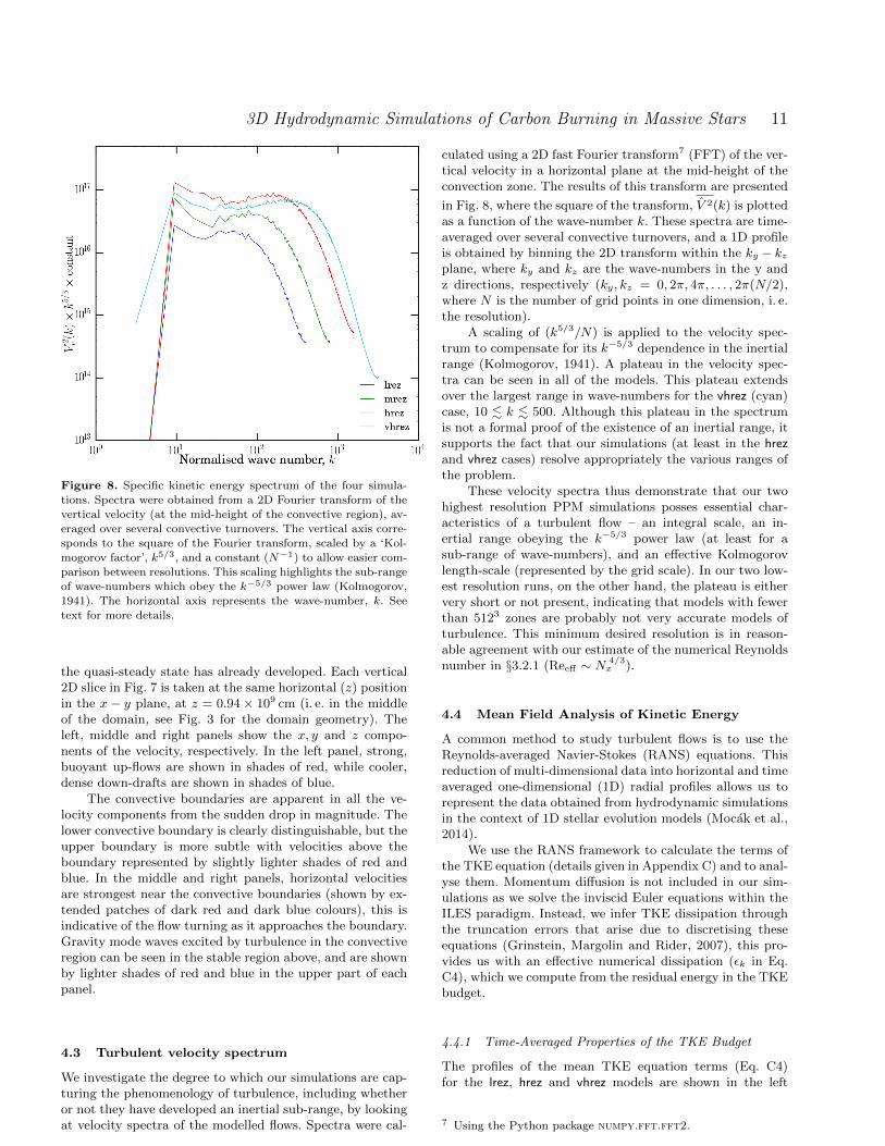
Figure 8. Specific kinetic energy spectrum of the four simula-

tions. Spectra were obtained from a 2D Fourier transform of thevertical velocity (at the mid-height of the convective region), av-

eraged over several convective turnovers. The vertical axis corre-

sponds to the square of the Fourier transform, scaled by a ‘Kol-mogorov factor’, 𝑘5/3, and a constant (𝑁−1) to allow easier com-

parison between resolutions. This scaling highlights the sub-rangeof wave-numbers which obey the 𝑘−5/3 power law (Kolmogorov,

1941). The horizontal axis represents the wave-number, 𝑘. See

text for more details.

the quasi-steady state has already developed. Each vertical2D slice in Fig. 7 is taken at the same horizontal (𝑧) positionin the 𝑥− 𝑦 plane, at 𝑧 = 0.94 × 109 cm (i. e. in the middleof the domain, see Fig. 3 for the domain geometry). Theleft, middle and right panels show the 𝑥, 𝑦 and 𝑧 compo-nents of the velocity, respectively. In the left panel, strong,buoyant up-flows are shown in shades of red, while cooler,dense down-drafts are shown in shades of blue.

The convective boundaries are apparent in all the ve-locity components from the sudden drop in magnitude. Thelower convective boundary is clearly distinguishable, but theupper boundary is more subtle with velocities above theboundary represented by slightly lighter shades of red andblue. In the middle and right panels, horizontal velocitiesare strongest near the convective boundaries (shown by ex-tended patches of dark red and dark blue colours), this isindicative of the flow turning as it approaches the boundary.Gravity mode waves excited by turbulence in the convectiveregion can be seen in the stable region above, and are shownby lighter shades of red and blue in the upper part of eachpanel.

4.3 Turbulent velocity spectrum

We investigate the degree to which our simulations are cap-turing the phenomenology of turbulence, including whetheror not they have developed an inertial sub-range, by lookingat velocity spectra of the modelled flows. Spectra were cal-

culated using a 2D fast Fourier transform7 (FFT) of the ver-tical velocity in a horizontal plane at the mid-height of theconvection zone. The results of this transform are presented

in Fig. 8, where the square of the transform, 𝑉 2(𝑘) is plottedas a function of the wave-number 𝑘. These spectra are time-averaged over several convective turnovers, and a 1D profileis obtained by binning the 2D transform within the 𝑘𝑦 − 𝑘𝑧plane, where 𝑘𝑦 and 𝑘𝑧 are the wave-numbers in the y andz directions, respectively (𝑘𝑦, 𝑘𝑧 = 0, 2𝜋, 4𝜋, . . . , 2𝜋(𝑁/2),where 𝑁 is the number of grid points in one dimension, i. e.the resolution).

A scaling of (𝑘5/3/𝑁) is applied to the velocity spec-trum to compensate for its 𝑘−5/3 dependence in the inertialrange (Kolmogorov, 1941). A plateau in the velocity spec-tra can be seen in all of the models. This plateau extendsover the largest range in wave-numbers for the vhrez (cyan)case, 10 . 𝑘 . 500. Although this plateau in the spectrumis not a formal proof of the existence of an inertial range, itsupports the fact that our simulations (at least in the hrezand vhrez cases) resolve appropriately the various ranges ofthe problem.

These velocity spectra thus demonstrate that our twohighest resolution PPM simulations posses essential char-acteristics of a turbulent flow – an integral scale, an in-ertial range obeying the 𝑘−5/3 power law (at least for asub-range of wave-numbers), and an effective Kolmogorovlength-scale (represented by the grid scale). In our two low-est resolution runs, on the other hand, the plateau is eithervery short or not present, indicating that models with fewerthan 5123 zones are probably not very accurate models ofturbulence. This minimum desired resolution is in reason-able agreement with our estimate of the numerical Reynoldsnumber in S3.2.1 (Reeff ∼ 𝑁

4/3𝑥 ).

4.4 Mean Field Analysis of Kinetic Energy

A common method to study turbulent flows is to use theReynolds-averaged Navier-Stokes (RANS) equations. Thisreduction of multi-dimensional data into horizontal and timeaveraged one-dimensional (1D) radial profiles allows us torepresent the data obtained from hydrodynamic simulationsin the context of 1D stellar evolution models (Mocak et al.,2014).

We use the RANS framework to calculate the terms ofthe TKE equation (details given in Appendix C) and to anal-yse them. Momentum diffusion is not included in our sim-ulations as we solve the inviscid Euler equations within theILES paradigm. Instead, we infer TKE dissipation throughthe truncation errors that arise due to discretising theseequations (Grinstein, Margolin and Rider, 2007), this pro-vides us with an effective numerical dissipation (𝜖𝑘 in Eq.C4), which we compute from the residual energy in the TKEbudget.

4.4.1 Time-Averaged Properties of the TKE Budget

The profiles of the mean TKE equation terms (Eq. C4)for the lrez, hrez and vhrez models are shown in the left

7 Using the Python package numpy.fft.fft2.

c○ 2017 RAS, MNRAS 000, 1–26


Figure 9. Left: Decomposed terms of the mean kinetic energy equation (Eq. C4), which have been horizontally averaged, normalised by

the domain surface area and time averaged over the steady-state period. Time averaging windows are over 2,200 s, 1,850 s and 1,000 s forthe lrez (top), hrez (middle) and vhrez (bottom) models, respectively. Right: Bar charts representing the radial integration of the profilesin the left panel. This plot is analogous to the middle panels of fig. 8 in Viallet et al. (2013).

c○ 2017 RAS, MNRAS 000, 1–26


panels of Fig. 9, with the inferred viscous dissipation shownby a black dashed line. These profiles are time integratedover multiple convective turnovers and normalised by thesurface area of the domain. Bar charts of the mean fieldsintegrated over the domain are shown in the right panels.Comparing the left panels of Fig. 9 to fig. 8 of Viallet et al.(2013), we see that the energetic properties of convectionduring carbon burning are very similar to oxygen burning.

Time Evolution. — The Eulerian time derivative of thekinetic energy, 𝜌Dt𝐸𝑘, is small or negligible over the simu-lation domain, implying that over the chosen time-scale themodel is in a statistically steady state.

Transport Terms. — The transport of kinetic energythroughout the convective region is determined by the twotransport terms, the TKE flux, Fk, and the acoustic flux,Fp (see Viallet et al., 2013, for a detailed discussion onthese terms).

Source Terms. — Turbulence is driven by two kineticenergy source terms, Wb and Wp. The rate of work dueto buoyancy, Wb (density fluctuations), is the main sourceof kinetic energy within the convective region, while Wp,the rate of work due to compression (pressure fluctuationsor pressure dilatation) is small. In the convective zone, wegenerally have Wb > 0, as expected since it is the maindriving term. Near the boundaries, however, there is aregion where Wb < 0. These regions are where the flowdecelerates (braking layer) as it approaches the boundary,as already found and discussed for oxygen burning inMeakin and Arnett (2007b) and Arnett et al. (2015). Wenote that the top braking layer is more extended than thebottom one. The top convective boundary width is alsomore extended. We come back to this point in S4.5.3.

Dissipation. — Kinetic energy driving is found to be closelybalanced by viscous dissipation, 𝜖𝑘; a property consistentwith the statistical steady state observed. The time and hor-izontally averaged dissipation can be seen to extend roughlyuniformly throughout the convective region but increasesslowly in its amplitude with depth, tracking the RMS ve-locities. There is almost no dissipation in the stable layers,where velocity amplitudes are low and turbulence is absent.Finally, there are notable peaks in dissipation localised atthe convective boundaries. The dependence of these peakson resolution is discussed next.

4.4.2 Resolution Dependence

We compare models of three different resolutions - the lrez,hrez and vhrez models, to determine if any of the physical re-sults depend on the chosen mesh size. Over the three resolu-tions, we find qualitatively similar results but there is signifi-cant deviation at the lower boundary region (∼ 0.9×109 cm).A key question is whether or not our higher resolution mod-els are able to capture the physics at boundaries accurately.

At the lower convective boundary (∼ 0.9 × 109 cm) apeak in dissipation appears at all resolutions (see dashed linein left panels of Fig. 9). The peak decreases in amplitude andwidth with increasing resolution, indicating that the modelsare not converged numerically.

A comparison of the dissipation in this region for allresolutions is given in the left panel of Figure 10. Here theTKE dissipation is normalised by a value at a common po-sition within the convective region near to the boundary.This highlights the relative decrease in this numerical peakwith respect to a converged value in the convective region. Asimilar plot for the upper boundary is presented in the rightpanel of Figure 10 shows that the dissipation at the bound-ary is smooth for both hrez and vhrez models. While in allcases the dissipation curves contain some variance due tothe stochastic nature of the flow, the trend with resolutionis clear.

4.5 Convective Boundary Mixing

Entrainment events (similar to entrainment events found foroxygen burning, see e. g. fig. 23 in Meakin and Arnett, 2007b)in the hrez model can be seen in the left panel of Fig. 11(see e. g. bottom left of convective zone where material frombelow the convective zone is entrained upwards or top cor-ners of the convective zones where the material is entrainedfrom the top stable layer). The left panel shows the aver-age atomic weight fluctuations relative to their mean, withthe velocity field in the (𝑥, 𝑦) plane over-plotted (the ver-tical axis corresponds to the radial/vertical direction, seeFig. 3). The right panel also shows the velocity magnitude(√

𝑣2𝑥 + 𝑣2𝑦) for the same snapshot of the hrez model. In bothpanels, strong flows can be seen in the centre of the con-vective region and shear flows can be seen over the entireconvective region. These shear flows have the greatest im-pact at the convective boundaries, where composition andentropy are mixed between the convective and radiative re-gions. Turbulent entrainment within the convective shell canalso be inferred through the radial profile of the buoyancywork, whereby the positive work near the boundaries (e.g.the magenta curve of Fig. 9 at ∼ 0.9 × 109 cm) implies thatthat TKE of overturning fluid elements near the boundarydoes work against gravity to draw stable material into theconvective region. This characteristic is explained in detailand seen in the buoyancy flux profiles of the oxygen burningshell in Meakin and Arnett (2007b) (see their S7.2 and thetop panel of fig. 25). This is a very different picture fromthe parametrisations that are used to describe convectiveboundary mixing in most modern 1D stellar evolution mod-els.

In this section, we start by estimating the position (andits time evolution) and thickness of the boundaries. We theninterpret the time evolution of the boundary positions in theframework of the entrainment law. Finally, we compare theupper and lower boundaries.

4.5.1 Estimating Convective Boundary Locations

Entrainment at both boundaries pushes the boundary posi-tion over time into the surrounding stable regions. In orderto calculate the boundary entrainment velocities, first theconvective boundary positions must be determined in thesimulations. In the 3D simulations, the boundary is a two-dimensional surface and is not spherically symmetric as in1D stellar models. In order to estimate the radial position ofa convective boundary we first map out a two-dimensional

c○ 2017 RAS, MNRAS 000, 1–26


0.88 0.90 0.92 0.94 0.96 0.98

Radius (109 cm)

0.0

1.0

2.0

3.0

4.0

5.0

6.0

7.0

8.0

ε k/ε

k,l

lrezmrezhrezvhrez

1.75 1.80 1.85 1.90 1.95 2.00

Radius (109 cm)

0.0

0.5

1.0

1.5

2.0

2.5

3.0

3.5

4.0

ε k/ε

k,u

lrezmrezhrezvhrez

Figure 10. Numerical dissipation inferred from the residual turbulent kinetic energy for the lower (left) and upper (right) convective

boundary regions in the lrez, mrez, hrez and vhrez models. The dissipation at each boundary has been normalised by a value at a common

position within the convective region near to the boundary. The hrez and vhrez residual profiles appear to be converging at the upperboundary, suggesting that the representative numerical dissipation here is physically relevant.

Figure 11. Left: Vertical cross-section of the absolute average atomic weight fluctuations relative to their mean within the convectiveregion. The colour map represents the logarithm of compositional fluctuations (|𝐴′

/𝐴0|) relative to the mean. Arrows show the verticalcomponent and one horizontal component of the velocity vector field, (𝑣𝑥, 𝑣𝑦) (the vertical axis corresponds to the radial/vertical direction,

see Fig. 3). The direction of the arrows indicates the direction of this vector field in the x-y plane, and their length the magnitude of

the velocity vector,√

𝑣2𝑥 + 𝑣2𝑦 , at that grid point. Right: Vertical cross-section of the same velocity vector field plotted as arrows in the

left panel. The colour-map represents the velocity magnitude in cm s−1. Both snapshots were taken at 2,820 s into the hrez simulation.

A movie of the velocity magnitude is available on this webpage: http://www.astro.keele.ac.uk/shyne/321D/convection-and-convective-boundary-mixing/visualisations/very-high-resolution-movie-of-the-c-shell/view.

horizontal boundary surface, 𝑟𝑗,𝑘 = 𝑟(𝑗, 𝑘), for 𝑗 = 1, 𝑛𝑦;𝑘 = 1, 𝑛𝑧, where 𝑛𝑦 and 𝑛𝑧 are the number of grid pointsin the horizontal 𝑦 and 𝑧 directions. We estimate the radialposition of the boundary at each horizontal coordinate tocoincide with the position where the average atomic weight,𝐴, is equal to the average between the mean value of 𝐴

in the convective and the corresponding radiative zones asdefined in Eq. A3. The standard deviation of the position,𝜎𝑟, represents the amplitude of the fluctuations of the ver-tical position of the boundary across the horizontal planedue to the fact the the boundary is not a flat surface. Ourmethod is a valid but not a unique way in which to cal-

c○ 2017 RAS, MNRAS 000, 1–26


culate the boundary position. See Sullivan et al. (1998);Fedorovich, Conzemius and Mironov (2004); Meakin andArnett (2007b); Liu and Ecke (2011); Sullivan and Patton(2011); van Reeuwijk, Hunt and Jonker (2011); Garcia andMellado (2014); Gastine, Wicht and Aurnou (2015) for a dis-cussion of alternative definitions. The time evolution of theboundary position and its standard deviation are plotted inFig. 13.

4.5.2 Convective Boundary Structure

While stellar evolution codes describe a convective boundaryas a discontinuity (see the composition profile in the rightpanel of Fig. 4, for example), 3D hydrodynamic simulationsshow a more complex structure. A boundary layer structureis formed between the convective and stably stratified re-gions. This can be seen from the apparent structure of themean fields, at ∼ 0.9×109 cm and ∼ 1.9×109 cm, in the leftpanels of Fig. 9, which represent the approximate locationsof the lower and upper convective boundaries, respectively.

The buoyancy in the convective boundary regions isnegative, as seen in the Wb profiles of Fig. 9. In these re-gions, approaching fluid elements are decelerated and radialvelocities greatly reduced. As horizontal velocities increase,the plumes turn around and fall back into the convectiveregion. This is similar to the description by Arnett et al.(2015) (see their fig. 5 and text therein).

4.5.3 Convective Boundary Thickness Estimates

We estimate the thickness of the convective boundaries us-ing the jump in composition, 𝐴, between convective andstable regions. We denote the average composition (averag-ing removes stochastic fluctuations in composition) in the,lower stable, convective and upper stable regions as, 𝐴𝑙, 𝐴𝑐

and 𝐴𝑢, respectively. We consider the boundary region toextend between 99% and 101% of the respective positionscoincident with such compositional values. For each bound-ary, we signify such values by the appendage of a subscript− (99%) or + (101%) to the composition of each region.Explicitly, the lower boundary thickness is defined as,

𝛿𝑟𝑙 = 𝑟(𝐴𝑐+

)− 𝑟

(𝐴𝑙−

). (14)

The upper boundary thickness is similarly defined as,

𝛿𝑟𝑢 = 𝑟(𝐴𝑢+

)− 𝑟

(𝐴𝑐−

). (15)

In addition, we also considered defining the boundarythickness using gradients in composition and entropy, andthe jump in entropy at the boundary. We found that theseother methods gave quantitatively similar results. In Fig. 12,we illustrate the estimation of the boundary thickness usingEqs. 14 and 15 for the final time-step of each simulation.The radius of each profile has been shifted, such that theboundary position, 𝑟 (see S4.5.1), of each model coincideswith the boundary position of the vhrez model. With such ashift, it is easier to assess the dependence of the boundaryshape on resolution.

The extents of the convective boundaries are markedby filled squares for each simulation. Filled circles representthe individual mesh points, indicating the resolution of each

Table 2. Table summarising bulk and boundary region prop-

erties for each model. 𝑣𝑟𝑚𝑠 - global RMS convective velocity(cm s−1); ℓ𝑐 - convective region height (cm); 𝑣𝑒 - entrainment

velocity (cm s−1); 𝛿𝑟 - boundary region width (cm); 𝛿𝑟/𝐻𝑝 - ra-

tio of the boundary region width to the average pressure scaleheight across the boundary; 𝜏𝑏 - boundary entrainment time (s);

RiB - bulk Richardson number. Values in brackets correspond to

the lower boundary.

lrez mrez hrez vhrez

𝑣𝑟𝑚𝑠 3.76 4.36 4.34 3.93(106)

ℓ𝑐 1.08 1.04 1.03 1.09(109)

𝑣𝑒 1.78 (-0.44) 2.01 (-0.39) 2.15 (-0.30) 1.59 (-0.46)(104)

𝛿𝑟 13.2 (10.3) 12.5 (5.1) 9.9 (3.3) 9.6 (2.9)(107)

𝛿𝑟/𝐻𝑝 0.41 (0.36) 0.36 (0.17) 0.29 (0.11) 0.28 (0.10)

𝜏𝑏 7.4 (23.4) 6.2 (13.1) 4.6 (11.0) 6.0 (6.3)

(103)

RiB 29 (370) 21 (259) 20 (251) 23 (299)

simulation. Note that, the composition profile labelled asmodel GENEC is from the 1D stellar model, and was usedas part of the initial conditions for all of the 3D models,so serves only as a qualitative comparison. The exact thick-ness of each boundary is shown in Table 2, along with theirfraction of the local pressure scale height.

In Fig. 12 (right panel), it can be seen that the com-position gradient at the top boundary is nearly convergedbetween all resolutions and varies only mildly between thelowest resolution case and the other models. The composi-tion gradient at the lower boundary (left panel), on the otherhand, varies significantly between the lrez and hrez models,while between the hrez and vhrez the boundary shape ap-pears to have nearly converged although is still narrowingslightly. These trends are confirmed by the quantitative es-timates of the boundary widths presented in Table 2.

The thickness determined from the abundance gradi-ents is larger than the standard deviation, 𝜎𝑟, of the bound-ary location (corresponding to the mid-points of the abun-dance gradients plotted in Fig. 12) shown as shaded areasin Fig. 13. This is expected since the fluctuations of theboundary location do not take into account its thickness orwidth, but only the location of its centre (mid-point). Thesefluctuations of the boundary location can be compared tofluctuations in the height of the ocean surface due to thepresence of waves. The fact that the width determined fromthe abundance gradients (given in Table 2) is significantlylarger means that there is mixing across the boundary. Apromising candidate for this type of mixing is the Kelvin-Helmholtz instability which would give rise to the shear mo-

c○ 2017 RAS, MNRAS 000, 1–26


0.80 0.82 0.84 0.86 0.88 0.90 0.92 0.94 0.96

Shifted Radius (109 cm)

14.0

14.5

15.0

15.5

16.0

16.5

17.0

17.5

18.0

18.5

A

vhrezhrezmrezlrezGENEC

1.85 1.90 1.95 2.00 2.0514.0

14.5

15.0

15.5

16.0

16.5

17.0

17.5

18.0

18.5

A

Figure 12. Radial compositional profiles at the lower (left) and upper (right) convective boundary regions for the last time step of eachmodel. The radius of each profile is shifted such that the boundary position, 𝑟 (see S4.5.1), coincides with the boundary position of the

vhrez model. In this sense, it is easier to assess the convergence of each model’s representation of the boundary at the final time-step.

Individual mesh points are denoted by filled circles. Approximate boundary extent (width) is indicated by the distance between two filledsquares for each resolution. The initial composition profile calculated using genec is shown in black (for a qualitative comparison only).

See the corresponding text (S4.5.3) for details of the definition of the boundary width.

tions seen in Fig. 14. This figure shows sequential slices of theflow velocity across the left section of the upper convectiveboundary region. Such shear mixing is induced by plumesrising from the bottom of the convective region and turningaround at the boundary (see also the shear layer in fig. 5 ofArnett et al., 2015). Mixing also occurs through plume im-pingement or penetration with the boundary. Some mixingmay also occur through the presence of gravity waves whichpropagate through the stable region. It is not expected thatthe upper boundary gradient will steepen, as this would sup-port more violent surface waves whose non-linear dissipationwould tend to broaden the gradient, resulting in a negativefeedback loop between these two processes.

It is important to remember that the boundary widthsgiven in Table 2 are only estimates. The key finding are (1)that the lower boundary has a narrower width compared tothe upper, and (2) the widths are relatively well convergedbetween the hrez and vhrez models.

4.5.4 Convective Boundary Evolution and EntrainmentVelocities

The variation in time of the average surface position, 𝑟, ofboth boundaries is shown for all models in Fig. 13. Positionsare shown as solid lines and twice the standard deviation asthe surrounding shaded envelopes. Following the initial tran-sient (> 1, 000 s) a quasi-steady expansion of the convectiveshell proceeds. We obtained the entrainment velocities, 𝑣𝑒,given in Table 2 using a linear fit to the time evolution of theboundary positions during the quasi-steady phase. These ve-

locities are very high. If one multiplies them by the life-timeof carbon shell burning (of the order of 10 years), the con-vective boundaries would move by more than 1010 cm, whichwould lead to dramatic consequences for the evolution of thestar. Note, though, that the driving luminosity of the shellwas boosted by a factor of 1,000. We will come back to thispoint in S4.6.

4.5.5 The Equilibrium Entrainment Regime

In the equilibrium entrainment regime (Fedorovich,Conzemius and Mironov, 2004; Garcia and Mellado, 2014),the time-scale for the boundary migration, 𝜏𝑏, is compa-rable to or larger than the turbulent transit time-scale, 𝜏𝑐(S3.3). Therefore, in this regime, the entrainment process issampling the entire spectrum of turbulent motions over theinertial range rather than being sensitive to individual tur-bulent elements, such as in strong, individual outliers events.This simplifies the development of mixing models within thisregime. The boundary entrainment velocity 𝑣𝑒 = 𝑑 𝑟/𝑑𝑡 isdefined in terms of the mean boundary position 𝑟(𝑡). We de-fine the boundary mixing time-scale as 𝜏𝑏 = 𝛿𝑟/|𝑣𝑒|, where𝛿𝑟 is the boundary thickness (Table 2), which we define inS4.5.3. We find 𝜏𝑏/𝜏𝑐 ratios for the upper convective bound-ary of 13.4, 13.1, 9.8 and 11.7 for the lrez, mrez, hrez andvhrez models, respectively, placing all of these boundariesfirmly in the equilibrium regime.

c○ 2017 RAS, MNRAS 000, 1–26


Figure 13. Time evolution of the mean radial position of the convective boundaries, averaged over the horizontal plane for all fourresolutions. Shaded envelopes are twice the standard deviation from the boundary mean location. The convective turnover time in these

simulations is of the order of 1,000 s. Top panel: Upper convective boundary region. For increasing resolution, the average standard

deviation, 𝜎𝑟, in the estimated boundary position are the following percentages of the local pressure scale height: 3.3%; 3.8%; 4.3%;and 4.5%. Bottom panel: Lower convective boundary region. For increasing resolution the average standard deviation in the estimated

boundary position are the following percentages of the local pressure scale height: 0.8%; 0.7%; 0.4%; and 0.6%. These shaded areasrepresent the variation in the boundary height due to the fact that the boundary is not a flat surface. This can be compared to the

surface of the ocean not being flat due to the presence of waves.

4.5.6 The Entrainment Law

The time rate of change of the boundary position due to tur-bulent entrainment (the entrainment velocity), 𝑣𝑒, has beenfound to scale as a power of the bulk Richardson number fora wide range of conditions (e. g. Garcia and Mellado, 2014).This relationship is often referred to as an entrainment lawin the meteorological and atmospheric and is typically writ-ten as:

𝑣𝑒𝑣𝑟𝑚𝑠

= 𝐴Ri−𝑛B . (16)

Many LES (e. g. Deardorff 1980) and laboratory (e. g.Chemel, Staquet and Chollet 2010) studies have found sim-ilar values for the coefficient, 𝐴, typically between 0.2 and0.25, although experimental measures have been more un-certain.

The exponent, 𝑛, is often found to be close to unity forconvectively driven turbulence (e. g. Fernando, 1991; Stevensand Lenschow, 2001), a result that follows from basic ener-getic considerations. On the other hand, in a recent DNSstudy, Jonker et al. (2013) showed that 𝐴 ≈ 0.35 and𝑛 = 1/2 for shear-driven entrainment.

We compare the bulk Richardson number (Eq. A5) ofour 3D simulations to the initial conditions from the 1Dstellar model (Cristini et al., 2016) and 3D oxygen burn-

ing simulations from Meakin and Arnett (2007b). From the1D 15 M⊙ stellar model of Cristini et al. (2016), used asinitial conditions in these simulations, the bulk Richardsonnumbers of the carbon burning shell are Ri𝑢B ∼ 1, 440 andRi 𝑙B ∼ 2.0 × 104 at the upper and lower convective bound-aries, respectively. While, for our 3D vhrez model (see Table2), we found Ri𝑢B ∼ 23 and Ri 𝑙B ∼ 299. The lower values weobtain in 3D are mainly due to the fact that we boosted theluminosity by a factor of 1,000. This is further discussed inS4.6.

The entrainment speed (normalised by the RMSvelocity) is plotted as a function of the bulk Richardsonnumber in Fig. 15. Red points represent the data obtainedin the study by Meakin and Arnett (2007b), the solid redline is a best fit power law to the data following a linearregression, and the red dashed lines show the error in thecomputed slope. Blue opaque points represent the valuesobtained in the hrez and vhrez models and blue transparentpoints are the values obtained in the lrez and mrez models.We obtain a best fit power law to the hrez and vhrez dataand the extremes of their error bars, shown by the solid blueline and dashed blue lines, respectively. The correspondingintercept and slope of this best fit denote the entrainmentcoefficient, 𝐴 = 0.03 (±0.01), and entrainment exponent,𝑛 = 0.62 (+0.09/− 0.15), respectively. The value we obtainfor the entrainment exponent, 𝑛, falls between the two

c○ 2017 RAS, MNRAS 000, 1–26


Figure 14. Sequential vertical cross-sections in the x-y plane of the velocity magnitude,√

𝑣2𝑥 + 𝑣2𝑦 + 𝑣2𝑧 , across the left section of the

upper convective boundary for the vhrez simulation. Snapshots are taken at 1565 s (upper left), 1570 s (upper right), 1575 s (lower left)

and 1580 s (lower right). The colour bar presents the values of the velocity magnitude in units of cm s−1. Each panel reveals shear mixingoccurring across the boundary interface. The Kelvin-Helmholtz instability is a promising candidate for generating this type of mixing.

scaling relations (1/2 6 𝑛 6 1). Our value for the coeffi-cient, 𝐴, however, differs from all of the values found in theliterature. A larger dataset is desired with which to explorein more detail the parameter space. Interestingly, the bulkRichardson numbers are similar between the carbon andoxygen shell models, and in particular, the lower convectiveboundaries both have higher values than the correspondingupper boundaries. The difference in the best fit valuesof 𝐴 indicates that the oxygen shell is more efficient inconverting kinetic energy into mixing. The difference in thebest fit values of 𝑛 indicates that there may be a secondparameter besides RiB that is varying between the topand bottom of the convective shells, and in different ways,between the carbon and oxygen shell models. Finally, itmust be reiterated that the ambiguity associated with cal-culating RiB is likely to account for some of the discrepancy.

4.5.7 Comparison of Upper and Lower ConvectiveBoundary Properties

Summarising the boundary properties determined so far forthe hrez model (see Table 2), the upper boundary regionhas a typical width of 9.9 × 107 cm, entrainment speed of2.2 × 104 cm s−1 and bulk Richardson number of 20. Thelower boundary region typically has a width of 3.3×107 cm,entrainment speed of 3 × 103 cm s−1 and bulk Richardsonnumber of 251. We thus have a consistent picture of the lowerboundary being narrower, having a slower entrainment ve-

locity and being stiffer (higher RiB) compared to the upperboundary by a factor of about 3, 7 and 13 respectively.

4.6 Comparing Convective Boundary MixingBetween 1D and 3D Models

Upon comparing our results to the 1D GENEC stellarevolution models, we find that our boundary widths aremuch larger and the boundary structures are very differentfrom those calculated using strict Ledoux or Schwarzschildboundaries. The results of this and similar 3D hydrody-namic studies (Meakin and Arnett, 2007b; Viallet et al.,2013; Woodward, Herwig and Lin, 2015; Arnett et al., 2015;Couch et al., 2015; Jones et al., 2017) call for improved con-vective boundary mixing prescriptions in 1D stellar evolu-tion models.

An approximate relation can be obtained between RiBand the luminosity, allowing the determination of convectiveboundary stiffness in 1D stellar models. Considering Eq. 16(with 𝑛 = 1), the relation 𝑣rms ∝ 𝐿1/3 (assuming 𝜖nuc ∼𝑣3rms/ℓ; Kolmogorov 1941, and 𝐿 =

∫𝜖nuc d𝑚) and that the

entrainment rate scales roughly linearly with the luminosityof the shell over the quasi-steady state (Jones et al., 2017),which implies that 𝑣𝑒 ∝ 𝐿, we obtain that RiB ∝ 𝐿−2/3. In-terestingly, we find the same dependence when starting fromthe formula for RiB (given in Eq. A5), considering that thebuoyancy jump remains constant (which is reasonable fora given initial stratification) and that 𝑣rms ∝ 𝐿1/3. Using

c○ 2017 RAS, MNRAS 000, 1–26


10 100 1000

RiB

-3.5

-3.0

-2.5

-2.0

-1.5

-1.0

-0.5

log(

v e/v

rms)

Figure 15. Logarithm of the entrainment speed for high Peclet

number simulations, normalised by the RMS turbulent velocityversus the bulk Richardson number. Red points represent data

obtained in the study by Meakin and Arnett (2007b) and blue

points represent data obtained in this study, transparent pointsrepresent the values for the lrez and mrez models, which are not

included in best fit power law shown by the blue solid line. Theblue dashed lines show the best fit to the extremes of the error

bars of the hrez and vhrez models. The red solid line is the best fit

power law from a linear regression of the oxygen shell data andthe red dashed lines show the error in the computed slope.

the relation RiB ∝ 𝐿−2/3, the boost of a factor of 1,000 inthe luminosity of our 3D models thus implies a reduction bya factor of 100 in RiB. This brings the values of the bulkRichardson number between our 3D and 1D models of thecarbon shell into a reasonable agreement (see S4.5.6). A com-plication involves calculating the buoyancy jump needed forthe bulk Richardson number since it is not precisely definedin a complex, stratified situation like a stellar interior – thelength-scale used for this integration is therefore somewhatarbitrary.

Another important point is that we confirm with the3D simulations that the lower boundary is stiffer than theupper boundary, by a factor of about 13 in terms of RiB. Thefact that the entrainment velocity at the lower boundary isa factor of about 7 smaller than at the upper boundary ispartly explained by the fact that the horizontal velocities atthe lower boundary are higher than at the upper boundary(see Fig. 6).

Theoretical relations like the entrainment law willbe needed to determine entrainment velocities for differ-ent burning stages and their various phases. This can beachieved by first estimating the bulk Richardson numberof a given convective boundary from the luminosity, as de-scribed above. Then, one can approximate a turbulent RMSvelocity using the velocity calculated from MLT or a simi-lar method. Finally, Eq. 16 can be used with suitable valuesfor the entrainment coefficient and exponent to estimate theentrainment velocity of the mentioned convective boundary(e. g. Deardorff 1980; Fernando 1991; Stevens and Lenschow

2001; Meakin and Arnett 2007b; Chemel, Staquet and Chol-let 2010).

5 COMPARISON TO OTHER SIMULATIONS

As found by Cristini et al. (2016) using the same 1D stellarmodel used for these hydrodynamic simulations, the lowerconvective boundary is stiffer than the upper boundary asdetermined by the bulk Richardson number. Our higher res-olution 3D models produce comparable results for the bulkRichardson number and for the hrez model we obtain valuesof 20 and 251 for the upper and lower boundaries, respec-tively.

Meakin and Arnett (2007b) simulated the oxygen shellof a 23 M⊙ star in spherical coordinates, also using theprompi code. The driving of the carbon shell we simulateis similar to their oxygen shell, owing to the fact that weboosted the luminosity. We find that the profiles of the ve-locity components are comparable between the two models.As shown by our Fig. 15 and their fig. 26, we find similarestimates of the bulk Richardson numbers, while the valuesof the constants 𝐴 and 𝑛 (from Eq. 16) differ, this is some-what expected as the oxygen shell engulfs the neon burningshell and complex multiple shell burning proceeds.

We obtain a turbulent kinetic energy budget that is inagreement with that of spherical simulations of the oxygenshell in a 23 M⊙ star by Viallet et al. (2013). In such an en-ergy budget we see a statistically steady state of turbulenceover four convective turnovers. Predominantly, this is drivenfrom the bottom of the shell by a positive rate of work dueto buoyancy and dissipated at the grid scale by a numericalviscosity.

In recent full 4𝜋 simulations of the oxygen burning shellin a 25 M⊙ star, Jones et al. (2017) find a 2𝜎 fluctuation intheir calculation of the convective boundary of 17% of thelocal pressure scale height. This is larger than the horizontalfluctuation in our estimation of the upper boundary of thecarbon shell; a 2𝜎 fluctuation of 4.3% of the local pressurescale height (Fig. 13). This difference could be due to themaximum tangential velocity gradient method that Joneset al. (2017) use to estimate the boundary positions, whichdiffers from the method described in S4.5.1. We find compa-rable magnitudes of the velocity components (see our Fig.6, and their fig. 11), and also similar Mach numbers for theflow (see our Table 1, and their table 1). This could be inpart due to the fact that our boosted energy generation rate(∼ 3 × 1012 erg g−1 s−1) is comparable to the rate used intheir PPMstar (Woodward, Herwig and Lin, 2015) simu-lations. The relative magnitude of the radial velocity com-ponent in Fig. 6 is higher than that of Jones et al. (2017),and our horizontal velocity does not possess the same sym-metry as their tangential velocity. The latter could be dueto the difference in geometries between the two simulations.Jones et al. (2017) also observe entrainment at the upperconvective boundary of their oxygen shell. Their velocityof the upper boundary due to entrainment is lower than theentrainment velocity we estimate by over an order of magni-tude. One reason for this difference could be that the oxygenshell boundary is much stiffer than the carbon shell bound-ary, due to a smaller jump in buoyancy over the boundary(RMS turbulent velocities are similar). We determined this

c○ 2017 RAS, MNRAS 000, 1–26


difference in boundary stability through the difference in thepeak squared Brunt-Vaisala frequencies. The value for theupper boundary of the carbon shell (∼ 0.05 rad s−2) is an or-der of magnitude smaller than that of the oxygen shell. Thiscould explain the order of magnitude difference in entrain-ment velocity assuming that the oxygen shell simulationsalso follow an entrainment law of the form of Eq. 16.

6 CONCLUSIONS

3D hydrodynamic simulations that represent the second car-bon shell of a 15 M⊙ star have been performed, using theprompi code. The initial conditions used were finely mappedprofiles of the carbon shell structure from a 15 M⊙, solarmetallicity, non-rotating stellar model calculated by Cristiniet al. (2016) using the genec code. The luminosity of the 3Dmodel was provided by a parameterised nuclear energy gen-eration rate, energy losses were also accounted for throughescaping neutrinos, using a specific neutrino production rate,although their effect was negligible. The luminosity of themodel was boosted by a factor of 1,000 in order to ease thetime needed to establish the turbulent velocity field, as dis-cussed in S3.2. The computational domain utilised a plane-parallel geometry within a Cartesian coordinate system andused a parameterised gravitational acceleration.

We tested the dependence of our set-up on the domainmesh size by computing models of four different resolutions:1283, 2563, 5123 and 10243. At these resolutions, approx-imate numerical Reynolds number of 650, 1600, 4000 and104, respectively are achieved in the convective zone (us-ing Eq. 11). This means that with the exception of the lrezmodel, all of the models reach the turbulent regime (Re𝑒𝑓𝑓& 1000). While a resolution of 5123 appears to produce aconverged result at the upper boundary; the stiffer, lowerboundary continues to change up to our highest resolutionmodel. An even higher resolution run is thus planned.

We observed entrainment of material at both convectiveboundaries for all of the models considered. This entrain-ment over the quasi-steady turbulent state is associated withan almost constant velocity, and the corresponding time-scale is greater than the time-scale for the largest fluid ele-ments to transit the convective region, asserting that convec-tive boundary mixing in these models occurs within the equi-librium entrainment regime. The average entrainment veloc-ities over the respective boundaries are 2.2×104 cm s−1 and−0.3×104 cm s−1 for the upper and lower boundary, respec-tively. We also found that the entrainment velocity scaleswith the stiffness (bulk Richardson number) of the convec-tive boundaries. This scaling follows the entrainment lawwith entrainment coefficient and exponent, 𝐴 = 0.03 (±0.01)and 𝑛 = 0.62 (+0.09/− 0.15), respectively. These constantswere obtained from only two convective boundaries. Addi-tional simulations using different initial conditions shouldhelp explore the parameter space of the entrainment law andwhether or not the parameters we derived vary significantlyfrom one burning stage to the other. Furthermore, the de-pendence on the Peclet number needs to be further exploredbefore our results obtained in the neutrino-cooled advancedphases can be applied to the early phases (hydrogen and he-lium burning) during which thermal effects are important,at least at the small scales (see discussion in Viallet et al.,

2015). We also estimated the boundary widths and foundthese to be roughly 30% and 10% of the local pressure scaleheight for the upper and lower convective boundary, respec-tively. While these widths are only estimates, they confirmthat the lower boundary is narrower than the upper bound-ary.

Although more 3D simulations of all burning stages areneeded to fully characterize convective boundary mixing, wecan already compare our results to those of previous studiesas well as the 1D input stellar model and relate them viameasures of the turbulent driving and boundary stiffness.For this purpose, we investigated how entrainment and tur-bulent velocities, the driving luminosity and boundary stiff-ness (measured using the bulk Richardson number) relate toeach other in S4.6. Considering these relations enabled us toreconcile the convective boundary properties of the carbonshell estimated from the initial 1D stellar evolution modelto the properties of boundaries in the 3D simulations pre-sented here (despite the artificial increase in luminosity forthe 3D simulations). Referring to the similarities betweencarbon and oxygen shell simulations presented in S5, a co-herent picture seems to emerge from all existing simulationsrelated to the advanced burning stages in massive stars whenconsidering the relations between the above quantities.

This is promising for the long term goal of developinga convective boundary mixing prescription for 1D modelswhich is applicable to all (or many) stages of the evolutionof stars (and not only to the specific conditions studied in3D simulations). The luminosity (driving convection) andthe bulk Richardson number (a measure of the boundarystiffness) will be key quantities for such new prescriptions(also see Arnett et al., 2015).

The goal of 1D stellar evolution models is to capturethe long-term (secular) evolution of the convective zone andof its boundaries, while 3D hydrodynamic simulations probethe short-term (dynamical) evolution. Keeping this in mind,the key points to take from this and previous 3D hydrody-namic studies for the development of new prescriptions in1D stellar evolution codes are the following:

∙ Entrainment of the boundary and mixing across it oc-curs both at the top and bottom boundaries. Thus 1D stellarevolution models should include convective boundary mix-ing at both boundaries. Furthermore, the boundary shapeis not a discontinuity in the 3D hydrodynamic simulationsbut a smooth function of radius, sigmoid-like, a feature thatshould also be incorporated in 1D models.

∙ At the lower boundary, which is stiffer, the entrainmentis slower and the boundary width is narrower. This confirmsthe dependence of entrainment and mixing on the stiffnessof the boundary.

∙ Since the boundary stiffness varies both in time andwith the convective boundary considered, a single constantparameter is probably not going to correctly represent thedependence of the mixing on the instantaneous convectiveboundary properties. As discussed above, we suggest theuse of the bulk Richardson number in new prescriptions toinclude this dependence.

c○ 2017 RAS, MNRAS 000, 1–26


ACKNOWLEDGEMENTS

The authors acknowledge support from EU-FP7-ERC-2012-St Grant 306901. RH acknowledges support from the WorldPremier International Research Centre Initiative (WPI Ini-tiative), MEXT, Japan. This article is based upon workfrom the ChETEC COST Action (CA16117), supported byCOST (European Cooperation in Science and Technology).This work used the Extreme Science and Engineering Dis-covery Environment (XSEDE), which is supported by Na-tional Science Foundation grant number OCI-1053575. CMand WDA acknowledge support from NSF grant 1107445at the University of Arizona. The authors acknowledge theTexas Advanced Computing Center (TACC) at The Uni-versity of Texas at Austin (http://www.tacc.utexas.edu)for providing HPC resources that have contributed tothe research results reported within this paper. MV ac-knowledges support from the European Research Councilthrough grant ERC-AdG No. 341157-COCO2CASA. Thiswork used the DiRAC Data Centric system at DurhamUniversity, operated by the Institute for ComputationalCosmology on behalf of the STFC DiRAC HPC Facility(www.dirac.ac.uk). This equipment was funded by BIS Na-tional E-infrastructure capital grant ST/K00042X/1, STFCcapital grants ST/H008519/1 and ST/K00087X/1, STFCDiRAC Operations grant ST/K003267/1 and Durham Uni-versity. DiRAC is part of the National E-Infrastructure.

APPENDIX A: 1D STELLAR CONVECTIONPARAMETERS

To determine averages over the convective region, we usedan RMS mass average. The mass average of a quantity 𝐴 isdefined as:

𝐴avg =

√1

𝑚2 −𝑚1

∫ 𝑚2

𝑚1

𝐴2(𝑚) 𝑑𝑚, (A1)

where 𝑚1 and 𝑚2 are the mass at the lower and upper con-vective boundaries, respectively.

The bulk Richardson number is the ratio of the bound-ary stabilising potential to the kinetic energy of turbulentmotions (within the convective region). It characterises theboundary stiffness, and is a function of the Brunt-Vaisalafrequency or buoyancy frequency, 𝑁 , which is defined as:

𝑁2 = −𝑔

(𝜕ln𝜌

𝜕𝑟

𝑒− 𝜕ln𝜌

𝜕𝑟

𝑠

), (A2)

where 𝑔 is the gravitational acceleration, 𝜌 is the density,and subscripts 𝑒 and 𝑠 represent the fluid element and itssurroundings, respectively.

In order to study the properties of the boundary re-gions, we first need a definition of the boundary location,𝑟𝑐. Meakin and Arnett (2007b) use the maximum gradientmethod on the composition to determine the location of con-vective boundaries in the oxygen shell of a 23 M⊙ model. In asimilar manner, we approximate the location of the top (bot-tom) boundary as the vertical coordinate having an averageatomic mass, 𝐴, equal to the average between the convectivezone and top (bottom) radiative zone,

𝐴𝑡ℎ =𝐴conv + 𝐴rad

2, (A3)

where 𝐴𝑐𝑜𝑛𝑣 and 𝐴𝑟𝑎𝑑 are the averages of 𝐴 in the convectiveand relevant stable/radiative regions, respectively.

The buoyancy jump over a convective boundary regioncan be estimated by integrating the square of the buoyancyfrequency over a suitable distance (∆𝑟) either side of theboundary centre, 𝑟𝑐,

∆𝐵 =

𝑟𝑐+Δ𝑟∫𝑟𝑐−Δ𝑟

𝑁2𝑑𝑟. (A4)

The integration distance ∆𝑟 is not well defined theoreti-cally but it should be large enough to capture the dynamicsof the boundary region and the distance over which fluidelements are decelerated.

As mentioned above, the bulk Richardson number is theratio of the boundary stabilisation potential (which includesthe buoyancy jump) to the kinetic energy due to turbulentmotions (within the convective region),

RiB =∆𝐵ℓ

𝑣𝑟𝑚𝑠2, (A5)

where ℓ is the integral length-scale which represents the sizeof the largest fluid elements. The integral length-scale is of-ten taken to be the horizontal correlation length. Meakin

c○ 2017 RAS, MNRAS 000, 1–26


Table A1. Estimates of the convective velocity (cm s−1), Bulk Richardson number, Mach number, Peclet number and Damkohler

number of different times during core and shell burning phases of a 15M⊙ stellar model. Bulk Richardson numbers are boundary values,

brackets indicate values at the lower boundary, all other values were mass averaged over the convective region. Peclet numbers are orderof magnitude estimates.

Phase 𝑣𝑐 (cm s−1) RiB Ma Pe Da

H Core Start 6.9×104 1.8×102 9.3×10−4 ∼ 103 3.8×10−8

H Core End 9.7×104 1.1×102 1.5×10−3 ∼ 103 7.2×10−7

He Core Start 4.7×104 1.2×103 4.3×10−4 ∼ 104 1.8×10−7

He Core Max 5.9×104 4.0×102 5.0×10−4 ∼ 105 3.5×10−6

He Core End 5.9×104 3.8×102 5.1×10−4 ∼ 105 3.0×10−6

C Core Start 6.9×104 7.2×103 3.0×10−4 ∼ 106 3.4×10−6

C Core Max 5.6×104 1.2×104 2.4×10−4 ∼ 107 1.2×10−5

C Core End 5.8×104 3.9×102 2.4×10−4 ∼ 107 1.8×10−5

Ne Core Start 1.5×106 82 3.9×10−3 ∼ 1010 3.3×10−3

Ne Core Max 6.4×105 3.6×102 1.9×10−3 ∼ 1010 5.5×10−3

Ne Core End 4.1×105 62 1.1×10−3 ∼ 1010 2.6×10−3

O Core Start 8.8×105 2.4×102 2.2×10−3 ∼ 1010 6.3×10−4

O Core Max 7.9×105 8.5×104 2.0×10−3 ∼ 1010 2.4×10−3

O Core End 7.5×105 27 1.8×10−3 ∼ 1010 2.0×10−3

He Shell Start 1.4×105 46 ( 20 ) 8.9×10−4 ∼ 106 5.7×10−8

He Shell End 1.3×105 14 ( 1.8×103 ) 9.1×10−4 ∼ 106 1.0×10−7

C Shell Start 3.6×105 4.2×102 ( 6.0×103 ) 1.3×10−3 ∼ 108 1.3×10−4

C Shell IC𝑎 2.9×105 6.9×102 ( 1.5×104 ) 1.2×10−3 ∼ 108 2.0×10−4

C Shell End 1.6×105 59 ( 6.5×104 ) 5.7×10−4 ∼ 107 1.3×10−4

O Shell Start 1.5×105 3.7×104 ( 4.0×104 ) 3.4×10−4 ∼ 1010 2.7×10−4

O Shell End 5.7×105 1.2×102 ( 3.4×104 ) 1.3×10−3 ∼ 1010 1.4×10−3

𝑎 Properties of the 1D model used as initial conditions for the 3D simulations

and Arnett (2007b) show that the horizontal correlationlength-scale and pressure scale height are similar to withina factor ∼ 3. So for our analysis we use the pressure scaleheight close to the boundary. The RMS velocity, 𝑣𝑟𝑚𝑠, repre-sents the velocity of the largest fluid elements carrying mostof the energy, which for the 1D simulations we approximateas the convective velocity,

𝑣𝑐 =

(𝐹𝑐

𝜌

) 13

, (A6)

where 𝐹𝑐 is the convective flux.In estimating the Mach number, we determine the

sound speed, 𝑐𝑠, using the Helmholtz EOS (Timmes andArnett, 1999; Timmes and Swesty, 2000),

Ma =𝑣𝑐𝑐𝑠

. (A7)

The Peclet number (Pe) is defined as the ratio of thetime-scale for advective transport to the time-scale for trans-port through diffusion. In the stellar case thermal diffusiondominates over molecular diffusion. For the deep interiorheat transfer plays a minor role, so typically Pe >> 1. Wedetermine the Peclet number using the following formula,

Pe =3𝐷𝑚𝑙𝑡

𝜒, (A8)

where 𝐷𝑚𝑙𝑡 is the diffusion coefficient calculated using MLT,𝐷𝑚𝑙𝑡 = 𝑣𝑚𝑙𝑡ℓ𝑚𝑙𝑡/3, 𝑣𝑚𝑙𝑡 and ℓ𝑚𝑙𝑡 are the mixing length ve-locity and mixing length parameter. 𝜒 is the thermal diffu-sivity, defined as,

𝜒 =16𝜎 𝑇 3

3𝜅 𝜌2 𝑐𝑝(A9)

c○ 2017 RAS, MNRAS 000, 1–26


Table A2. Constants used in the fitting functions (Eq. B1) for the five sections of the entropy, 𝐴 and 𝑍 profiles. Subscripts 1, 2 and 3refer to the lower stable, convective and upper stable sections, respectively. Subscripts 𝑙 and 𝑢 refer to the lower and upper convective

boundary sections, respectively.

𝛼1 𝛽1 𝜃𝑙 𝜑𝑙 𝜂𝑙 𝛼2 𝛽2 𝜃𝑢 𝜑𝑢 𝜂𝑢 𝛼3 𝛽3

𝑠 1.65× 108 0.24 2.81× 108 3.43× 108 −0.5 3.43× 108 0 3.43× 108 3.56× 108 −0.5 3.56× 108 0.08

𝐴 18.17 0 18.17 16.19 0.5 16.19 0 16.19 14.38 0.5 14.38 0

𝑍 9.07 0 9.07 8.08 0.5 8.08 0 8.08 7.18 0.5 7.18 0

where 𝜎 is the Stefan-Boltzmann constant, 𝑇 the tempera-ture, 𝜅 the Rosseland mean opacity and 𝑐𝑝 the specific heatcapacity at constant pressure.

The Damkohler number (Da) is defined as the ratio ofthe advective time-scale to the nuclear reaction time-scale,generally this is small in deep convective regions as the time-scale for nuclear reactions is long, but during the advancedstages of massive star evolution the two time-scales can be-come comparable. We determine the Damkohler number us-ing the following formula,

Da =𝑡con𝑡nuc

=

(2ℓ𝑐𝑣𝑐

)(𝑞𝑋𝑖

𝜖𝑛𝑢𝑐

)−1

, (A10)

where 𝑡con is the convective turnover time and 𝑡nuc is therelevant nuclear reaction time-scale. ℓ𝑐 is the height of theconvective zone, 𝑞 is the specific energy released for the dom-inating reactions, 𝑋𝑖 is the mass abundance of the interact-ing particles and 𝜖𝑛𝑢𝑐 is the nuclear energy generation rate.

The majority of these variables are presented in TableA1 for most of the convective boundaries shown in Fig. 1.

APPENDIX B: STELLAR MODEL PROFILEFITTING

The entropy (𝑠), average atomic mass (𝐴) and averageatomic number (𝑍) were remapped by considering five dis-tinct sections of the domain. The lower stable region (belowthe lower convective boundary), the convective region andthe upper stable region (above the upper boundary) were fit-ted linearly in the form 𝛼+𝛽 𝑥, where 𝛼 and 𝛽 are constants,and 𝑥 is the radius on a grid point. The two remaining sec-tions are the upper and lower convective boundaries, thesewere fitted using sigmoid functions, 𝑓𝑠𝑖𝑔, of the form,

𝑓𝑠𝑖𝑔 = 𝜃 +𝜑− 𝜃

1 + 𝑒 𝜂 𝑧, (B1)

where 𝜃, 𝜑 and 𝜂 are constants, and 𝑧 is a normalisedgrid index. The fitting constants for the three variables arepresented in Table A2, the subscripts for each constant rep-resent the section of the domain for which the fit refers to.Subscripts 1, 2, 3 denote the lower stable, convective and up-per stable sections, respectively. Subscripts 𝑙 and 𝑢 refer tothe lower and upper convective boundary sections, respec-tively.

APPENDIX C: RANS TERMINOLOGY ANDTHE TURBULENT KINETIC ENERGYEQUATION

In the Reynolds-averaged Navier Stokes (RANS) framework,variables are split into mean and fluctuating components.The horizontally averaged mean is denoted by angled brack-ets and defined as,

⟨𝑎⟩ =1

∆𝐴

∫Δ𝐴

𝑎 𝑑𝐴, (C1)

where 𝑑𝐴 = 𝑑𝑦 𝑑𝑧 and ∆𝐴 = ∆𝑦∆𝑧 is the area of thecomputational domain. The fluctuating component, 𝑎′, isobtained by subtracting the mean of the variable from thevariable: 𝑎′ = 𝑎− ⟨𝑎⟩.

In order to statistically sample the quasi-steady statewe perform temporal averaging over several convectiveturnovers, denoted by an over-bar and defined as,

𝑎 =1

∆𝑡

∫ 𝑡2

𝑡1

𝑎(𝑡) 𝑑𝑡, (C2)

for an averaging window ∆𝑡 = 𝑡2 − 𝑡1.The Eulerian equation of turbulent kinetic energy can

be written as (eq. A12 of Meakin and Arnett 2007b):

𝜕𝑡 (𝜌𝐸𝑘) + ∇ · (𝜌𝐸𝑘𝑣) = −𝑣 ·∇𝑝 + 𝜌𝑣 · 𝑔 (C3)

where 𝑣 is the velocity and 𝐸𝑘 = 12(𝑣 · 𝑣) is the specific

kinetic energy.

Applying horizontal and temporal averaging to Eq. C3yields the mean turbulent kinetic energy equation, whichcan be written as,

⟨𝜌Dt𝐸𝑘⟩ = −∇ · ⟨Fp + Fk⟩

+ ⟨Wp⟩ + ⟨Wb⟩ − 𝜖𝑘,(C4)

where Dt = 𝜕𝑡 + ∇ · 𝑣 is the material derivative,Fp = 𝑝′𝑣′ is the turbulent pressure flux,Fk = 𝜌𝐸𝑘𝑣

′ is the turbulent kinetic energy flux,Wp = 𝑝′∇ · 𝑣′ is the pressure dilatation,Wb = 𝜌′𝑔 · 𝑣′ is the work due to buoyancy and𝜖𝑘 is the numerical dissipation of kinetic energy.

c○ 2017 RAS, MNRAS 000, 1–26


REFERENCES

Alexander, D. R. and J. W. Ferguson. 1994. “Low-temperature Rosseland opacities.” ApJ 437:879–891.

Almgren, A. S., J. B. Bell and M. Zingale. 2007.“MAESTRO: A Low Mach Number Stellar Hydrody-namics Code.” Journal of Physics Conference Series78(1):012085.

Angulo, C., M. Arnould, M. Rayet, P. Descouvemont,D. Baye, C. Leclercq-Willain, A. Coc, S. Barhoumi, P.Aguer, C. Rolfs, R. Kunz, J. W. Hammer, A. Mayer, T.Paradellis, S. Kossionides, C. Chronidou, K. Spyrou, S.degl’Innocenti, G. Fiorentini, B. Ricci, S. Zavatarelli, C.Providencia, H. Wolters, J. Soares, C. Grama, J. Rahighi,A. Shotter and M. Lamehi Rachti. 1999. “A compilationof charged-particle induced thermonuclear reaction rates.”Nuclear Physics A 656:3–183.

Arnett, D. 1994. “Oxgen-burning hydrodynamics. 1:Steady shell burning.” ApJ 427:932–946.

Arnett, D. 1996. Supernovae and Nucleosynthesis: An In-vestigation of the History of Matter from the Big Bang tothe Present.

Arnett, W. D. 1968. “Explosive Ignition of Carbon in Starsof Intermediate Mass.” Natur. 219:1344–1346.

Arnett, W. D. and C. Meakin. 2011a. “Toward RealisticProgenitors of Core-collapse Supernovae.” ApJ 733:78.

Arnett, W. D. and C. Meakin. 2011b. “Turbulent Cells inStars: Fluctuations in Kinetic Energy and Luminosity.”ApJ 741:33.

Arnett, W. D. and C. Meakin. 2016. “Key issues re-view: numerical studies of turbulence in stars.” Reportson Progress in Physics 79(10):102901.

Arnett, W. D., C. Meakin and M. Viallet. 2014. “Chaos andturbulent nucleosynthesis prior to a supernova explosion.”AIP Advances 4(4):041010.

Arnett, W. D., C. Meakin, M. Viallet, S. W. Campbell,J. C. Lattanzio and M. Mocak. 2015. “Beyond Mixing-length Theory: A Step Toward 321D.” ApJ 809:30.

Asida, S. M. and D. Arnett. 2000. “Further Adventures:Oxygen Burning in a Convective Shell.” ApJ 545:435–443.

Aspden, A., N. Nikiforakis, S. Dalziel and J. Bell. 2008.“Analysis of implicit LES methods.” ”Communications inApplied Mathematics and Computational Science” 3:103–126.

Audouze, J., C. Chiosi and S. E. Woosley. 1986. Nucle-osynthesis and chemical evolution. In Saas-Fee AdvancedCourse 16: Nucleosynthesis and Chemical Evolution, ed.J. Audouze, C. Chiosi and S. E. Woosley.

Bazan, G. and D. Arnett. 1994. “Convection, nucleosyn-thesis, and core collapse.” ApJ 433:L41–L43.

Bazan, G. and D. Arnett. 1997. “Large Nuclear Networksin Presupernova Models.” Nuclear Physics A 621:607–610.

Bazan, G. and D. Arnett. 1998. “Two-dimensional Hydro-dynamics of Pre–Core Collapse: Oxygen Shell Burning.”ApJ 496:316–332.

Beaudet, G., V. Petrosian and E. E. Salpeter. 1967. “En-ergy Losses due to Neutrino Processes.” ApJ 150:979.

Boldyrev, S. and F. Cattaneo. 2004. “Magnetic-Field Gen-eration in Kolmogorov Turbulence.” Physical Review Let-ters 92(14):144501.

Chemel, C., C. Staquet and J.-P. Chollet. 2010. “Estimat-ing the diffusive heat flux across a stable interface forced-

newpage by convective motions.” Nonlinear Processes inGeophysics 17:187–200.

Colella, P. and P. R. Woodward. 1984. “The Piece-wise Parabolic Method (PPM) for Gas-Dynamical Sim-ulations.” J. Comput. Phys. 54:174–201.

Couch, S. M., E. Chatzopoulos, W. D. Arnett and F. X.Timmes. 2015. “The Three-dimensional Evolution to CoreCollapse of a Massive Star.” ApJ 808:L21.

Cristini, A., C. Meakin, R. Hirschi, D. Arnett, C. Georgyand M. Viallet. 2016. “Linking 1D evolutionary to 3Dhydrodynamical simulations of massive stars.” Phys. Scr.91(3):034006.

Damkohler, Gerhard. 1940. “Der Einfluss der Turbu-lenz auf die Flammengeschwindigkeit in Gasgemischen.”Zeitschrift fr Elektrochemie und angewandte physikalischeChemie 46(11):601–626.

de Jager, C., H. Nieuwenhuijzen and K. A. van der Hucht.1988. “Mass loss rates in the Hertzsprung-Russell dia-gram.” A&AS 72:259–289.

Deardorff, J. W. 1980. “Stratocumulus-capped mixed lay-ers derived from a three-dimensional model.” Boundary-Layer Meteorology 18:495–527.

Denissenkov, P. A., F. Herwig, J. W. Truran and B. Paxton.2013. “The C-flame Quenching by Convective BoundaryMixing in Super-AGB Stars and the Formation of HybridC/O/Ne White Dwarfs and SN Progenitors.” ApJ 772:37.

Denissenkov, P. A., F. Herwig, L. Bildsten and B. Paxton.2013. “MESA Models of Classical Nova Outbursts: TheMulticycle Evolution and Effects of Convective BoundaryMixing.” ApJ 762:8.

Eggenberger, P., G. Meynet, A. Maeder, R. Hirschi, C.Charbonnel, S. Talon and S. Ekstrom. 2008. “The Genevastellar evolution code.” Ap&SS 316:43–54.

Fedorovich, E., R. Conzemius and D. Mironov. 2004. “Con-vective Entrainment into a Shear-Free, Linearly Strati-fied Atmosphere: Bulk Models Reevaluated through LargeEddy Simulations.” J. Atmos. Sci. 61:281.

Fernando, H. J. S. 1991. “Turbulent mixing in stratifiedfluids.” Annual Review of Fluid Mechanics 23:455–493.

Freytag, B., H.-G. Ludwig and M. Steffen. 1996. “Hydro-dynamical models of stellar convection. The role of over-shoot in DA white dwarfs, A-type stars, and the Sun.”A&A 313:497–516.

Fryxell, B., E. Muller and D. Arnett. 1989. Computation ofmulti-dimensional flows with non-uniform composition. InNuclear Astrophysics, ed. W. Hillebrandt and E. Muller.p. 100.

Fryxell, B., K. Olson, P. Ricker, F. X. Timmes, M. Zingale,D. Q. Lamb, P. MacNeice, R. Rosner, J. W. Truran andH. Tufo. 2000. “FLASH: An Adaptive Mesh Hydrody-namics Code for Modeling Astrophysical ThermonuclearFlashes.” ApJS 131:273–334.

Garcia, J. and J. Mellado. 2014. “The two-layer structure ofthe entrinament zone in the convective boundary layer.”J. Atmos. Sci. pp. 1935–1955.

Gastine, T., J. Wicht and J. M. Aurnou. 2015. “TurbulentRayleigh-Benard convection in spherical shells.” J. FluidMech. 778:721–764.

Georgy, C., H. Saio and G. Meynet. 2014. “The puzzle ofthe CNO abundances of 𝛼 Cygni variables resolved by theLedoux criterion.” MNRAS 439:L6–L10.

Gilet, C., A. S. Almgren, J. B. Bell, A. Nonaka, S. E.

c○ 2017 RAS, MNRAS 000, 1–26


Woosley and M. Zingale. 2013. “Low Mach Number Mod-eling of Core Convection in Massive Stars.” ApJ 773:137.

Grinstein, F., L. Margolin and W. Rider. 2007. ImplicitLarge Eddy Simulation - Computing Turbulent Fluid Dy-namics.

Jones, S., R. Andrassy, S. Sandalski, A. Davis, P. Wood-ward and F. Herwig. 2017. “Idealized hydrodynamic sim-ulations of turbulent oxygen-burning shell convection in4𝜋 geometry.” MNRAS 465:2991–3010.

Jones, S., R. Hirschi, K. Nomoto, T. Fischer, F. X. Timmes,F. Herwig, B. Paxton, H. Toki, T. Suzuki, G. Martınez-Pinedo, Y. H. Lam and M. G. Bertolli. 2013. “AdvancedBurning Stages and Fate of 8-10 M Stars.” ApJ 772:150.

Jonker, Harm J. J., Maarten van Reeuwijk, Peter P. Sul-livan and Edward G. Patton. 2013. “On the scaling ofshear-driven entrainment: a DNS study.” Journal of FluidMechanics 732:150–165.

Kolmogorov, A. 1941. “The Local Structure of Turbulencein Incompressible Viscous Fluid for Very Large Reynolds’Numbers.” DoSSR 30:301–305.

Kolmogorov, A. N. 1962. “A refinement of previous hy-potheses concerning the local structure of turbulence ina viscous incompressible fluid at high Reynolds number.”Journal of Fluid Mechanics 13:82–85.

Kuhlen, M., W. E. Woosley and G. A. Glatzmaier. 2003.3D Anelastic Simulations of Convection in Massive Stars.In 3D Stellar Evolution, ed. S. Turcotte, S. C. Keller andR. M. Cavallo. Vol. 293 of Astronomical Society of thePacific Conference Series p. 147.

Kuranz, C. C., H.-S. Park, B. A. Remington, R. P. Drake,A. R. Miles, H. F. Robey, J. D. Kilkenny, C. J. Keane,D. H. Kalantar, C. M. Huntington, C. M. Krauland, E. C.Harding, M. J. Grosskopf, D. C. Marion, F. W. Doss, E.Myra, B. Maddox, B. Young, J. L. Kline, G. Kyrala, T.Plewa, J. C. Wheeler, W. D. Arnett, R. J. Wallace, E.Giraldez and A. Nikroo. 2011. “Astrophysically relevantradiation hydrodynamics experiment at the National Ig-nition Facility.” Ap&SS 336:207–211.

Lautrup, B. 2011. Physics of Continuous Matter: Ex-otic and Everyday Phenomena in the Macroscopic World.CRC press.

Liu, Y. and R. E. Ecke. 2011. “Local temperature measure-ments in turbulent rotating Rayleigh-Benard convection.”Phys. Rev. E 84(1):016311.

Lorenz, E. N. 1963. “Deterministic Nonperiodic Flow.” J.Atmos. Sci. 20:130–148.

Maeder, A. 2009. Physics, Formation and Evolution ofRotating Stars.

Maeder, A., G. Meynet, N. Lagarde and C. Charbonnel.2013. “The thermohaline, Richardson, Rayleigh-Taylor,Solberg-Høiland, and GSF criteria in rotating stars.”A&A 553:A1.

Martins, F. and A. Palacios. 2013. “A comparison of evo-lutionary tracks for single Galactic massive stars.” A&A560:A16.

Meakin, C. A. 2006. Hydrodynamic modeling of massivestar interiors. PhD thesis University of Arizona, (2006).

Meakin, C. A. and D. Arnett. 2006. “Active Carbon andOxygen Shell Burning Hydrodynamics.” ApJ 637:L53–L56.

Meakin, C. A. and D. Arnett. 2007a. “Anelastic and Com-pressible Simulations of Stellar Oxygen Burning.” ApJ

665:690–697.Meakin, C. A. and D. Arnett. 2007b. “Turbulent Con-vection in Stellar Interiors. I. Hydrodynamic Simulation.”ApJ 667:448–475.

Miernik, J., G. Statham, L. Fabisinski, C. D. Maples, R.Adams, T. Polsgrove, S. Fincher, J. Cassibry, R. Cortez,M. Turner and T. Percy. 2013. “Z-Pinch fusion-basednuclear propulsion.” Acta Astron. 82:173–182.

Mocak, M., C. Meakin, M. Viallet and D. Arnett. 2014.“Compressible Hydrodynamic Mean-Field Equations inSpherical Geometry and their Application to TurbulentStellar Convection Data.” ArXiv e-prints .

Muller, B., M. Viallet, A. Heger and H.-T. Janka. 2016.“The Last Minutes of Oxygen Shell Burning in a MassiveStar.” ApJ 833:124.

Porter, D. H. and P. R. Woodward. 2000. “Three-dimensional Simulations of Turbulent Compressible Con-vection.” ApJS 127:159–187.

Prialnik, D. 2000. An Introduction to the Theory of StellarStructure and Evolution.

Rogers, F. J., F. J. Swenson and C. A. Iglesias. 1996.“OPAL Equation-of-State Tables for Astrophysical Ap-plications.” ApJ 456:902.

Schaller, G., D. Schaerer, G. Meynet and A. Maeder. 1992.“New grids of stellar models from 0.8 to 120 solar massesat Z = 0.020 and Z = 0.001.” A&AS 96:269–331.

Schwarzschild, K. and H.-H. Voigt. 1992. GesammelteWerke / Collected Works.

Stevens, B. and D. H. Lenschow. 2001. “Observations, Ex-periments, and Large Eddy Simulation.” Bulletin of theAmerican Meteorological Society 82:283–294.

Stothers, R. B. and C.-W. Chin. 1991. “Metal opacitiesand convective core overshooting in Population I stars.”ApJ 381:L67–L70.

Sullivan, P. P., C.-H. Moeng, B. Stevens, D. H. Lenschowand S. D. Mayor. 1998. “Structure of the Entrain-ment Zone Capping the Convective Atmospheric Bound-ary Layer.” J. Atmos. Sci. 55:3042–3064.

Sullivan, P. P. and E. G. Patton. 2011. “The Effect ofMesh Resolution on Convective Boundary Layer Statisticsand Structures Generated by Large-Eddy Simulation.” J.Atmos. Sci. 68:2395–2415.

Sytine, I. V., D. H. Porter, P. R. Woodward, S. W. Hod-son and K.-H. Winkler. 2000. “Convergence Tests for thePiecewise Parabolic Method and Navier-Stokes Solutionsfor Homogeneous Compressible Turbulence.” Journal ofComputational Physics 158:225–238.

Tayar, J., G. Somers, M. H. Pinsonneault, D. Stello,A. Mints, J. A. Johnson, O. Zamora, D. A. Garcıa-Hernandez, C. Maraston, A. Serenelli, C. Allende Prieto,F. A. Bastien, S. Basu, J. C. Bird, R. E. Cohen, K. Cunha,Y. Elsworth, R. A. Garcıa, L. Girardi, S. Hekker, J. Holtz-man, D. Huber, S. Mathur, S. Meszaros, B. Mosser, M.Shetrone, V. Silva Aguirre, K. Stassun, G. S. Stringfellow,G. Zasowski and A. Roman-Lopes. 2017. “The Correla-tion Between Mixing Length and Metallicity on the GiantBranch: Implications for Ages in the Gaia Era.” ArXiv e-prints .

Timmes, F. X. and D. Arnett. 1999. “The Accuracy, Con-sistency, and Speed of Five Equations of State for StellarHydrodynamics.” ApJS 125:277–294.

Timmes, F. X. and F. D. Swesty. 2000. “The Accuracy,

c○ 2017 RAS, MNRAS 000, 1–26


Consistency, and Speed of an Electron-Positron Equationof State Based on Table Interpolation of the HelmholtzFree Energy.” ApJS 126:501–516.

Turner, J. S. 1973. Buoyancy Effects in Fluids.van Dyke, M. 1982. “An album of fluid motion.” NASASTI/Recon Technical Report A 82.

van Reeuwijk, M., G. R. Hunt and H. J. Jonker. 2011. Di-rect simulation of turbulent entrainment due to a plumeimpinging on a density interface. In Journal of PhysicsConference Series. Vol. 318 of Journal of Physics Confer-ence Series p. 042061.

Viallet, M., C. Meakin, D. Arnett and M. Mocak. 2013.“Turbulent Convection in Stellar Interiors. III. Mean-fieldAnalysis and Stratification Effects.” ApJ 769:1.

Viallet, M., C. Meakin, V. Prat and D. Arnett. 2015. “To-ward a consistent use of overshooting parametrizations in1D stellar evolution codes.” A&A 580:A61.

Vink, J. S., A. de Koter and H. J. G. L. M. Lamers. 2001.“Mass-loss predictions for O and B stars as a function ofmetallicity.” A&A 369:574–588.

Woodward, P. R., F. Herwig and P.-H. Lin. 2015. “Hy-drodynamic Simulations of H Entrainment at the Top ofHe-shell Flash Convection.” ApJ 798:49.

Young, P. A., C. Meakin, D. Arnett and C. L. Fryer. 2005.“The Impact of Hydrodynamic Mixing on Supernova Pro-genitors.” ApJ 629:L101–L104.

Zahn, J.-P. 1991. “Convective penetration in stellar interi-ors.” A&A 252:179–188.

This paper has been typeset from a TEX/ LATEX file preparedby the author.

c○ 2017 RAS, MNRAS 000, 1–26

Documents

A. Cristini , C. Meakin , arXiv:1610.05173v2 [astro-ph.SR ... · PDF file3D Hydrodynamic Simulations of Carbon Burning in Massive Stars 3 quires a large additional computational e