Embed Size (px)
Citation preview
Journal of Financial Economics 4 (1977) 129-176. (0 North-Holland Publishing Company
A CRITIQUE OF THE ASSET PRICING THEORY’S TESTS
Part I: On Past and Potential Testability of the Theory*
Richard ROLL* l
University of California, Los Angeles, CA 90024, U.S.A.
Received June 1976, revised version received October 1976
Testing the two-parameter asset pricing theory is difficult (and currently infeasible). Due to a mathematical equivalence between the individual return/beta’ linearity relation and the market portfolio’s mean-variance efficiency, any valid test presupposes complete knowledge of the true market portfolio’s composition. This implies, inter alia, that every individual asset must be included in a correct test. Errors of inference inducible by incomplete tests are discussed and some ambiguities in published tests are explained.
If the horn honks and the mechanic concludes that the whole electrical system is working, he is in deep trouble. . .
Pirsig (1974)
1. Introduction and summary
The two-parameter asset pricing theory is testable in principle; but arguments are given here that: (a) No correct and unambiguous test of the theory has appeared in the literature, and (b) there is practically no possibility that such a
*This is Part I of a three-part study. Parts 11 and III are summarized in the introduction here. but will appear in later issues. A copy of the complete paper can be obtained by writing the author at: Graduate School of Management, University of California, Los Angeles, CA 90024. USA.
**This paper was written while the author was at the Centrc d’Enseignement Sup&ieur des Afl’aires. France. Eugene Fama, Michael C. Jensen, John B. Long, Jr., Stephen Ross and Bruno H. Solnik provided many useful comments and Patricia Porter provided excellent secretarial service. While the paper was being written, Fama pointed out that his new book (1976) contains some of the same analysis and conclusions. New papers by Stephen Ross (forthcoming) and John B. Long (1976) contain results emphasized, and formerly believed to have been discovered, here. The reader will be able to verify, however, that most of this material is non-redundant.
To the authors criticised hem: these papers were singled out because they are the best and most widely read on the subject. I have written some papers in this area too and have taught the subject to a numbcr,of unsuspecting students. So, the absence of detailed self-criticism should be attributed to the greater importance of the other papers and does not imply any personal prescicncc. None was present.
130 R. Roll, Critique of asset pricing theory tests - I
test can be accomplished in the future. This broad indictment of one of the three fundamental paradigms of modern finance will undoubtedly be greeted by my colleagues, as it was by me, with scepticism and consternation. The purpose of this paper is to eliminate the scepticism. (No relief is offered for the consternation.)
Here are the paper’s conclusions:
(1) There is only a single testable hypothesis associated with the generalized two-parameter asset pricing model of Black (1972). This hypothesis is: ‘the market portfolio is mean-variance efficient’.
(2) All other so-called implications of the model, the best known being the linearity relation between expected return and ‘beta’, follow from the market portfolio’s efficiency and are not independently testable. There is an ‘if and only if’ relation between return/beta linearity and market portfolio mean- variance efficiency.
(3) In any sample of observations on indivjdual returns, regardless of the gener- ating process, there will always be an infinite number of ex-post mean- variance efficient portfolios. For each one, the sample ‘betas’ calculated between it and individual assets will be exactly linearly related to the in - dividual sample mean returns. In other words, if the betas are calculated against such a portfolio, they will satisfy the linearity relation exac+ whether or not the true market portfolio is mean-variance efficient. (The same properties also hold ex ante, of course). These results are implied in earlier literature [e.g., Ross (1972)], but I do not believe that their full consequences have been adequately explored previously. Some of these consequences are:
(4) The theory is not testable unless the exact composition of the true market portfolio is known and used in the tests. This implies that the theory is not testable unless all individual assets are included in the sample.
(5) Using a proxy for the market portfolio is subject to two difficulties. First the proxy itself might be mean-variance efficient even when the true market portfolio is not. This is a real danger since every sample will display efficient portfolios that satisfy perfectly all of the theory’s implications. For example, suppose there exist 1000 assets but only 500 are used in the sample. For the sample, there will exist well-diversified portfolios of the 500 assets that seem to be reasonable proxies for the market and for which observed returns are exactly linearily related cross-sectionally to observed betas. On the other hand, the chosen proxy may turn out to be inefficient; but obviously, this alone implies nothing about the true market portfolio’s efficiency. Further- more, most reasonable proxies will be very highly correlated with each other and with the true market whether or not they are mean-variance efficient. This high correlation will make it seem that the exact composition is un- important, whereas it can cause quite different inferences.
R. Roll, Critique of asset pricing theory tests - I 131
(6) As a case in point, a detailed discussion is provided of the papers by Fama and MacBeth (1973). Black, Jensen, and Scholes (1972) and Blume and Friend (1973), in the context of their rejection of the Sharpe-Lintner model. It is shown that their tests results are fully compatible with the Sharpe- Lintner model and a specification error in the measured ‘market’ portfolio. A misspecification would have created bias and non-stationarity in the fitted cross-sectional risk/return lines even if there were a constant riskless return. For the Black, Jensen and Scholes data, for example, there was a mean- variance efficient ‘market’ proxy that supported the Sharpe-Lintner model perfectly and that had a correlation of 0.895 with the market proxy actually employed. However, it cannot be ascertained without further analysis whether this other portfolio satisfied all the requirements of a good market proxy (such as positive proportions invested in all assets).
The market portfolio identification problem constitutes a severe limitation to the testability of the two-parameter theory. No two investigators who disagree on the market’s measured composition can be made to agree on the theory’s test results. However, suppose that advances in electronic monitoring of human capital and other non-traded assets make the market portfolio’s true composition knowable; or more realistically, suppose a given composition is just agreed upon by everyone relevant. How should the mean-variance efficiency of this known composition portfolio be tested? Part II of the paper (to appear in a later issue) investigates the peculiar econometric problems associated with such testing, viz. :
(7) A direct test of the proxy’s mean-variance efftcicncy is difficult computa- tionally because the full sample covariance matrix of individual returns must be inverted and statistically because the sampling distribution of the efficient set is generally unknown. Some possible solutions to the statistical problems are presented. They include tests based on the fact that the market portfolio must have positive proportions invested in all assets; large sample distribution-free tests; and tests based on the sampling distribution of the efficient set assuming Gaussian returns.
(8) Testing for the proxy’s efficiency by using the return/beta linearity relation also poses empirical difficulties:
(a) The two-parameter theory does not make a prediction about para- meter values but only about the form (linear) of the cross-sectional relation. Thus, econometric procedures designed to obtain accurate parameter estimates are not very useful.
(b) Specifically, the widely-used portfolio grouping procedure can support ’ the theory even when it is false. This is because individual asset deviations from exact linearity can cancel out in the formation of
132 R. Roll, Critique of asset pricing theory tests - I
portfolios. (Such deviations are not necessarily related to betas.) Some simulated data given by Miller and Scholes (1972) were used as an example of such an occurrence. Deviations in these data were known to be related to generating process asymmetry which would not have been detectable in grouped observations.
(9) Several others tests are proposed for the linearity relations. These include: (a) An Aitken-type procedure that gives unbiased cross-sectional tests
with individual assets, and (b) a procedure that exploits asymptotic exact linearity by measuring
the rate of decrease of cross-sectional residual variance with respect to increasing time-series sample size.
In Part III of the paper (to appear in a future issue), some of the common uses of the two-parameter theory are called into question:
(10) Deviations from the return/beta linearity relation are frequently linked with some other phenomenon. The validity of such linkages is criticised using the Jensen measure of portfolio performance as an example. If the ‘market* proxy used in the calculations is exactly (not significantly different from) ex-post efficient, all of the individual Jensen performance measures gross of expenses will be identically (not significantly different from) zero. They can be (significantly) non-zero only if the proxy market portfolio is (significantly) not effcieni. But if the proxy market portfolio is not efficient, what is the justification for using it as a benchmark in performance evalua- tion?
(11) The beta itself is criticiscd as a risk measure on two grounds: first, that it will always be (significantly) positively related to observed average in- dividual returns if the market index is on (not significantly off) the positively sloped section of the ex-post efficient frontier, regardless of inoesfors’ attirudes toward risk; and second, that it depends, non-monotonically, on the particular market proxy used. About the second point: if two in- vestors happen to choose two different ‘market’ portfolios, both of which are mean-variance efficient, the same security might have a beta of 1.5 for the first investor and 0.5 for the second. This is intuitively obvious since beta is supposed to be a relatioe measure of risk. But less obvious is the fact that if both investors increase the proportions this security re- presents in their ‘markets’, its beta will change and it can increase for one investor and decrease for another.
An appendix to this part (I) contains a compact analytic derivation of the efficient set propositions and includes a few original results (e.g., identity of the efficient portfolio that maximizes cross-sectional variation in beta).
R. Roll, Critique of assef pricing theory tests - I 133
2. The testable feature of asset pricing theory and the features that have been ‘tested’
2.1. Eficient set mathematics
We should begin any quantitative enquiry by setting forth the relationships that are mutually and logically equivalent. The mathematics of the mean- variance efficient set serves just such a purpose, for it exposes several logically- equivalent relations among mean returns and covariances (which are the building blocks of the asset pricing theory). The mathematics is mostly available else-
where [see, e.g., Sharpe (1970), Merton (1972), Black (1972), SzegS (1973, Fama (1976), Long (1976)l and a compact statement of all the familiar results plus some new ones is provided in the appendix.
The efficient set mathematics has been discussed most usually in terms of ex-ante returns and covariances. To emphasize the purely mathematical nature of the results, however, I should like to state it in terms of an observed sample of returns on N assets. No presumption is made about the population that generated this sample. It can be any probability law imaginable. Furthermore, no mention need be made about equilibrium, risk aversion, homogeneous anticipations, or anything else like that. There are only two assumptions:
(A.]) The sample product-moment covariance matrix, V, is non-singular.
(A.2) At least one asset had a different sample mean return from others.
These are very weak assumptions. (A.l) simply rules out assets whose returns were constant during every period in the sample and it excludes any pair of linear combinations of assets that were perfectly correlated during the sample period. (A.2) merely requires some sample variation in the critical variable of interest. After all, it is cross-sectional variation in the mean return which asset pricing theory strives to explain.
Given the sample covariance matrix and the arithmetic sample mean returns
(expressed as an N x 1 column vector R), the sample frontier of efficient ex-post portfolios can be easily obtained. This frontier enumerates all the portfolios that had minimal sample variance for each given level of mean sample return. Suppose we choose one of these portfolios, say portfolio m, with sample return r which lies on the positively-sloped part of the efficient frontier. (That is, t:Lre is no other portfolio with the same sample variance that had a higher
mean return.) Then the following statements are true:
(S.1) There exists a unique portfolio, denoted z, that had a correlation of zero with m during the sample period and that lies on the negatively-sloped
segment of the sample efficient frontier; this implies that the sample
131
(S.2)
R. Roll, Critique of asset pricing theory tests - I
return of m was greater than that of z, r,,, > rr. (For a formal proof, see the appendix, Corollary 3.)
For any arbitrary asset or portfolio, say j, the sample mean return is equal to a weighted average of rz and r, where the weight of m is exacfly the sample linear regression slope coefficient ofj on m, i.e.,
where
rJ E (1 -Pj>r,+Bjrm, for all j, (1)
s, = sample covariance of j and m
sample variance of m
(Proof: Appendix, Corollary 6).
Statement (S.l) is related to the following facts:
(S.3) Every portfolio on the positively-sloped segment of the sample efficient set was positively correlated with every other one (Corollary 4).
(S.4) Every sample efficient portfolio except the global minimum sample variance portfolio has an orthogonal portfolio with finite mean return (Corollary 3).
It is easy to see that (S.3) and (S.4) imply that r,,, > rz because we have chosen m to lie in the positively-sloped segment of the sample eficient frontier.
Proposition S.2, on the other hand follows from:
(S.5) The investment proportions of any sample efficient portfolio can be expressed as a weighted average of the proportions in any other two sample efticient portfolios whose means are different (Corollary 5).
Given (SJ), it is a simple matter to prove (1); see the appendix or, e.g., Black (1972, p. 450). In fact, a more general proposition than (1) follows readily from (S.5). Let A and B be any two arbitrary sample efficient portfolios, ex-post correlated or not, but with different sample mean returns. Then:
(S.6) The mean return on any arbitrary asset, j, is given exactly by
rJ = (I-&)rA+&B, for all j (4
(Corollary 6.A).
R. Roll, Critique of asset pricing theory tests - I 135
In eq. (2) Bi is the multivariate sample slope coefticient for B from the regression of rj on r, and rB. Furthermore, this regression coefficient has a simple form,
B; = k,i, - ~,4lmml- ~,43,
where bik is the sample covariance of i and k. It is easy to see that (1) is merely a special case of (2) that obtains when A is chosen to be B’s orthogonal sample portfolio.
Expression (2) can be considered a logical equivalent to assumptions (A.l) and (A.2). In other words, given an observed non-singular sample covariance matrix and at least two different sample mean returns, every observed mean return has exactly the relation shown in (2). Equivalently, every observed sample ‘beta’ conforms exactly to the rearrangement of (l),
A converse statement is also true:
(S.7) Let fl be the (Nx 1) column vector of simple regression slope coefficients computed between individual assets and some portfolio m. Then the vector of mean returns R is an exact linear function of the vector /3 only if m is a sample e5cient portfolio; i.e., in general,
R = rr I+@,,,-rJ/?, (4)
if and only if rm is ex-post efficient [r, is the mean return on m’s corres- ponding e5cient orthogonal portfolio and I is the unit vector, see Ross (1972, 1973)].
It follows that mean returns are not exact linear functions of betas when m is not enicicnt. This does not imply that mean returns are necessarily related to non-linear functions of beta. They are just not exacrly linear. For example, the relation
R = a+gj?
is a possibility if m is inefficient; where a is a vector whose elements are non- constant but are unrelated to the elements of p, and g is a scalar constant.
Before going on to the theory of asset pricing, it is well to emphasize the nature of these mathematical relations, Identity symbols have been used in (1) through (4) because they really are identities. Given the choice of m as ex-post efficient, these expressions hold exactly. They do not, therefore, provide any information about the state of nature or about the process that generated the
136 R. Roll, Critique of asset pricing theory tests - I
sample. The underlying probability law might be anything and the relations above would always be observed ex-post. This has relevant implications for testing the asset pricing theory, as we shall see.
2.2. A redew of some asset pricing theory tests
Three widely-quoted empirical papers on asset pricing theory are Black, Jensen and &holes (1972), Blume and Friend (1973), and Fama and MacBetb (1973).’ Let us examine what they said they were testing: The statement in Fama and MacBeth is very clear. They refer to a portfolio m which is on the ex-ante efficient frontier as seen by a single investor. This leads to the derivation of an equation identical to (1) but with investors* subjective parameters instead of sample parameters. The resulting equation [Fama-MacBeth (1973, p. 610)]
8 . . . has three testable implications: (Cl) the relationship between the expected returns on a security and its risk in any efficient portfolio m is linear. (C.2) /?, is a complete measure of the risk of security i in the efficient portfolio m; no other measure of the risk of i appears in (6) [eq. (1) here]. (C.3) in a market of risk-averse investors, higher risk should be associated with higher return; that is E(&,,)-E(&,) > 0.’ [RO is the same as rr here.]
Given that the word ‘risk’ has replaced the parameter /?, we have already seen that Fama and MacBeth’s (C. 1), (C.2). and (C.3) are simply implications of the fact that m is assumed ex-ante efficient. 2 If m is known to be efficient, these relations are not independently testable. They are tautological. When m is ellicient, the expected return must be linear in p and E(fl,) must exceed E(K,). Incidentally, given the assumption that m is efficient, their last inequality has nothing to do with risk aversion. It is purely the mathematical implication of the assumption about m and the definition of p. It is totally independent of investor preferences since it follows from the mathematical property (S.l). Conversely, if Fama and MacBeth’s (C.1) is true, and ex-ante /I is an exact linear function of ex-ante expected return, then m must be ex-ante mean-variance efficient.
It is clear from the authors’ discussion that they are aware of these internal
‘There are other interesting papers containing similar tests. e.g., Petit and Westerfjeld (1974) and Modigliani. Pogue. Scholes and Solnik (1972). Petit and Weslerfield’s test of the asset pricing theory is actually identical lo Black, Jensen and Scholes’ although Petit and Wateriield seem 10 deny this. Modigliani. Pogue, Scholes and Solnik carry out a similar test for eight different European stock markets. Palacios(l973)and Rosa(l975) present detailed investigations for Spain and France respectively. Roll (1973) gives a comparative test of the asset pricing theory and the optimal growth model using the same methodology. Set also Fama and MacBcth (1974a). Fama and Macbeth (1974b) investigate the extension of amt pricing theory jnto a multi-period context. Roll and Solnik (1975) apply the methodology to exchange rates.
‘(C.2). the statement that no other risk measure except /J is important, presupposes that /I measures risk. Whether it measures risk or not. however, it is the only variable on the right side of (1). (r. and r, are constant cross-sectionally.) Thus, it is the only cross-sectional explanatory variable of any kind.
R. Roll, Critique of asset pricing theory tests - I 137
relations. For example, on page 609 they state, ‘. . . there are conditions on expected returns that are implied by the fact that in a two-parameter world investors hold efficient portfolios.’ But on page 610 they make a statement inconsistent with the facts and with their own knowledge of the mathematics: ‘To test conditions (C.lHC.3) we must identify some efficient portfolio m.’ Of course, if m is identified as efficient, there is no need to test (C.lt(C.3). (See also the self-contradictory second paragraph on p. 614.)
But there are testable hypotheses in the Fama-MacBeth paper. The hypotheses really are :
(H.1) Investors regard as optimal those particular investment portfolios that are mean-variance efficient.
Assuming identical probability assessments by all investors, this hypothesis leads to:
(H.2) The ‘market portfolio’ is ex-ante efficient.
The ‘market portfolio’ is defined as a value-weighted combination of all assets (p. 611). Fama and MacBeth credit Black (1972) with deducing (H.2) given (H.1) and given homogeneous investor expectations. The Black proof is quite simple: Since all investors have identical beliefs and hold efficient port- folios, every investor holds a linear combination of two arbitrary efficient port- folios. Since the market portfolio is by construction a linear combination of the portfolios of individual investors, it is also a linear combination of these two efficient portfolios and is therefore also efficient [because the linear combination of any two efficient portfolios is also efflcicnt by the basic mathematical property of the efficient set, (SS)]. Interestingly, Black states that Lintner (1969) ‘. . . has shown that removing [the] assumption [of homogeneous anticipations] does not change the structure of capital asset prices in any significant way’ (p. 445). Nevertheless, Black’s proof of the market portfolio’s efficiency does require homogeneity. This might be relaxed in a more general (and as yet unknown) proof; but Fama (1976, ch. 7) has argued that, in fact, no equilibrium model with non-homogeneous anticipations is testable.’
‘On page 447 at the beginning of his discussion of efficient portfolios, Black makes a state- ment that seems to be in conflict with the results here. He claims that Cass and Stiglitz (1970) have shown
4 . . . that if the returns on securities are not assumed to be joint normal, but are allowed to lx arbitrary, then the set of efficient portfolios can be written as a weighted combination of two basic portfolios on/y for a special class of utility functions’ (italics added).
It is clear from his subsequent discussion that Black was referring to mean-ouriunce efficient portfolios. Thus, his statement is false. Efficient mean-variance portfolios can n/ways be con- structed as a ‘weighted combination of two basic portfolios’. Furthermore Cass and Stiglitz never claimed the contrary. What they did was to enumerate the set of utility functions for
138 R. Roll, Critique of asset pricing theory tests - I
In both the Black paper and the Fama-MacBeth paper there exists a bit of unfortunate wording about the efficient set mathematics and about optimal investment choices. At first, it might seem that the resulting confusion would be only niinor. But when it comes to empirical testing and to specifying exactly those relations that are empirically rejectable and are valid scientific hypotheses, this possible confusion is of great significance.
The only viable (i.e., rejectable) hypothesis that we have so far been able to uncover is (H.2), the market portfolio is mean-variance efficient.4 The assump- tions which are sufficient for this result are rather strong: Perfect capital markets, homogeneous anticipations, two-parameter probability distributions of returns. But there is also another assumption that has received little attention in the literature: namely, the market portfolio must be identifiable.
This last assumption is very important when we consider that there will always be some portfolio which is ex-post efficient and will bring about exact observed linearity among ex-post sample mean returns and ex-post sample betas. If we do not know the composition of the market portfolio, we might by chance select a proxy that is close to mean-variance efficient. In fact, it may be hard to find a highly-diversified portfolio that is sufficiently far inside the ex-post efficient frontier to permit the detection of statistically significant departures from mean return/beta exact linearity. We will return to this point later. First, let us see what some of the other papers have been testing.
The widely-quoted paper by Black, Jensen, and Scholcs (1972) makes no mention of the possible efficiency of the market portfolio and its importance for the linear relation between return and ‘beta’. In fact, however, the authors modestly claim that their ‘. . . main emphasis has been to test the strict traditional form of the asset pricing model’ (p. 113). by which they mean the original Sharpe (1964), Lintner (1965) model similar to (I), but with rr replaced by a ‘risklcss’ return. [This modci results from the asset pricing theory assumptions listed above, and used by Black to derive (I), plus the extra assumption that investors can borrow and lend as much as they like at a riskless interest rate.] Black, Jensen, and Scholes explicitly deny that they have provided tests of any other hypothesis. However, the Black model is clearly in the backs of their minds and on page 81 they even go so far as to provide a historical glimpse of Black’s theoretical progress by asserting that he ‘was able’ to derive his model
which all investors would construct their optimal portfolios as a weighted average of two basic portfolios. Under a restrictive set of preferences, each investor would regard a mean-variance efficient portfolio as optimal; but as Cass and Stiylitz show, there are other investor preferences which would lead lo ‘separation’ (or the choice of an optimal portfolio which is a weighted combination of two others). under which the optimal portfolio is not mean-variance efficient. [See also Hakansson (1969). Jacob (1970) and Ross (1976). The last reference gives separa- tion results for probability distributions instead of utility functions.]
4Fama and MacBeth also provide an ingenious time-series test of market competition, given the hypothesis (H.2). However, this part of their paper is about a different set of hypo- theses than our subject here.
R. Roll, Critique of asset pricing theory tests - I 139
‘after we had observed this phenomena’ (that mean returns are linearly related to calculated beta coefficients but supposedly with a different slope and intercept than those implied by the Sharpe-Lintner theory). The graphs plotted by Black, Jensen, and Scholes appear to portray a very linear mean return/beta relation over long sample periods. Unlike Fama and MacBeth, however, no formal test of linearity is provided. (It must not have seemed necessary given the authors’ goal.) Thus, no formal information is given on the possible efficiency of the measured market portfolio, nor about the hypothesis (H.2).
4 direct test of linearity was provided by one of the authors [Jensen (1972a, 1972b)], who, using the same data as those used by Black, Jensen and Scholes, presented results from a regression similar to the one later computed by Fama and MacBeth. In fact, the fitted equations are nearly identical in form but the measurement methods were somewhat different and the ‘market’ portfolios used in calculating betas were different. ’ This was evidently sufficient to create some disparity between the two sets of results. We cannot ascertain the exact extent of the disparity because the sub-periods reported in the two papers were not identical. At least the signs of coefficients on squared beta terms were in agreement, being negative during the longer sample periods. The statistical significance of these negative signs is less clear. For example, the coefficient given by Fama-MncBeth for the squared beta term during 1946-55 was -0.0076 (p. 623). The same coefiicient given by Jensen for an overlapping period, July 1948 to March 1957, was -0.0055. The associated f-statistics were far apart, howcvcr, Fams-MacBcth’s was -2.16 whereas Jensen’s was only -0.524.6 This difTcrcncc may very well be due to Fama and MacBcth’s presumably more powerful test but thcrc is no way to bc sure without a complete replication.
It might be worthwhile carrying out such a replication because the linearity is directly rclatcd to the market portfolio’s eficicncy. We can already be sure that the ‘market’ portfolios used by Jensen and by Fama and MacBeth did not lie exactly on the sample eCient frontier. If they had been exactly efficient, the relation between the mean r&urn vector and the vector of sample betas would have been exactly linear and it was not. ’ But it is not necessary for the basic hypothesis (H.2) (the market portfolio is ex-ante efficient) that the observed market portfolio be exactly ex-post eficient in every period. It only needs to be ellicient over ‘sufXciently’ long periods. Now both Jensen and Fama-MacBeth find no significant non-linearity over the longest sample period nor do they find
‘Cf. Jensen (1972b. pp. 385-388) with Fama and MacBcth (1973, pp. 615-617). ‘Jensen reported a r-statistic with rcspcct to a non-zero theoretical value which he derived
from Merton’s (1973) continuous time model. The number above is his I-statistic for a hypo- thesized coefficient of zero.
‘Actually, this is not entirely true for Fama-MacBcth since they did not USC concfdrrenl sample mean returns and betas. Thus, some deviation from linearity might have been observed in their results, cvcn if the ‘market’ portfolio had been exactly sample efficient, because the sample betas might not have been stationary. Part II of this paper will examine the importance for testing the basic hypothesis of attempting to purge measurement errors from sample betas. (This was the reason Fama and MacBeth did not use concurrent observations.)
140 R. Roll, Critique of asset pricing theory tests - I
any significance for non-beta ‘measures of risk’ such as standard deviation. Although this is consistent with their market portfolio proxies having been sample efficient over the long term, it is also consistent with their proxies having been inefficient (as we will soon see).
Interestingly, Fama and MacBeth offer a possible explanation for the sig- nificance of non-linear beta terms during some sample periods: viz., they suggest that there are omitted variables from the theory for which the non-linear terms act as proxies. Of course, their results are also consistent with the simpler explanation that the Fama-MacBeth ‘market’ portfolio was not exactly ex-post efficient in every sub-period. This alone implies that non-linear terms could be significant. It is also true that the non-exact ex-post efficiency of the market might induce significance in individual standard deviations (i.e., in non-portfolio risk measures).
2.3. Tests of the Sharpe-Lintner model
Let us now turn to an ancillary examination of the evidence offered by Black, Jehsen and Scholes and by others against the original Sharpe-Lintner theory. It will be useful to have the following supplementary results from the efficient set mathematics.
Given the following additional assumption:
(A.3) There exists an asset whose return was a constant, rr, during the sample period.
Then :
(S.7)
(S.8)
The sample efficient set (in the mean-variance space) is a parabola with a tangent on the return axis at rF.
Suppose we denote the ‘risky efficient set’ as the ensemble of portfolios with minimum variance excluding asset F. Then results (S. 1) through (S.6) still hold for the portfolios composing this ‘risky efficient set’.
In particular, for any ex post portfolio composed entirely of risky assets and lying on the positively-sloped segment of the ‘risky efficient set’, sample mean returns on all assets are exact linear functions of sample betas as portrayed by eq. (1); sample mean r, in (1) is the return on a portfolio lying on the negatively- sloped segment of the risky efficient set whose return was uncorrelated with the return on m during the sample period.
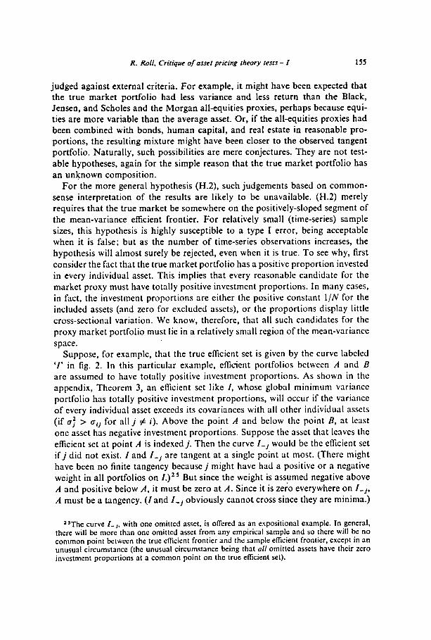
In other words, we have the familiar diagram shown in fig. 1, where m, m+ and z are all portfolios composed of risky assets only and are all on the sample risky efficient boundary. The portfolio m* is the sample ‘tangent’ portfolio
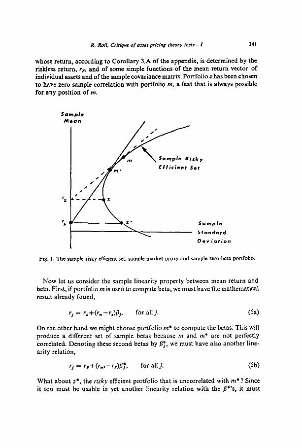
R. Roll, Critique of asset pricing theory tests - I 141
whose return, according to Corollary 3.A of the appendix, is determined by the riskless return, r,, and of some simple functions of the mean return vector of individual assets and of the sample covariance matrix. Portfolio z has been chosen to have zero sample correlation with portfolio m, a feat that is always possible for any position of m.
SCWlPlO Mean
Efficient Set
Sample
Deviation
Fig. 1. The sample risky efficient set, sample market proxy and sample zero-beta portfolio.
Now let us consider the sample linearity property between mean return and beta. First, if portfolio m is used to compute beta, we must have the mathematical result already found,
‘1 = f, + km - r.WJ. for all j.
On the other hand we might choose portfolio m+ to compute the betas. This will produce a different set of sample betas because m and M* are not perfectly correlated. Denoting these second betas by /I;, we must have also another line- arity relation,
‘J = rp + (fine - rJD;, for all j.
What about z*, the risky efficient portfolio that is uncorrelated with m* ? Since it too must be usable in yet another linearity relation with the /?*‘s, it must
142 R. Roll. Critique of asset pricing theory tests - I
have the same mean return as rP In fact, it is quite easy to prove that this is SO.’
Furthermore, since there is an infinite number of efficient risky portfolios along the positively-sloped boundary, there is an infinite number of these linearity relations, all equally satisfied exactly (but all with different beta vectors). In particular, rr and r,,, would have their own p: and Bz in (5b) and would satisfy the second linearity relation above. Note that j?: must be noncero because e5cient orthogonal portfolios are unique. Thus, even though m and z are uncorrelated, m* and z must be correlated. Furthermore, although m*‘s ortho- gonal portfolio is constrained to have the same sample return as the riskless return, there is no such restriction on portfolio z. Depending on the relative positions of m and m*, rr can be greater or less than rF.9
Armed with these purely logical results which are true for any sample satisfy- ing assumptions (A.l), (A.2), and (A.3), let us turn to the published tests of the original Sharpe-Lintner theory. First, what are the principal hypotheses of this theory? They are:
(H.3) Investors can borrow or lend at the riskless rate, rF.
(H.!) (Same as before.) They consider that mean-variance efficient portfolios arc optimal.
Thus, each individual would compose his portfolio of the risklcss asset F and his subjective tangent portfolio m *. If investors had homogeneous prob- ability assessments, they would all have the same tangent portfolio. Thus:
(H.4) The cx-ante efficient tangent portfolio is the market portfolio of all assets.
Of course, since there seems to be littlc possibility of rcjccting (H.3) or even (H.l) with direct information, we arc left with (H.4) as the testable hypothesis.
Black, Jensen, and Scholes rejected the Sharpe-Lintncr theory as a result of the following ‘test’: First, a ‘market’ portfolio was chosen and sample betas were calculated via a procedure designed carefully to remove measurement error. Then, the cross-sectional mean return/beta linearity relation was csti-
“By Corollary 3.A of the appendix, a tangent drawn to any point p on the efficient frontier intersects the return axis at the level of the mean return on p’s orthogonal portfolio. Since m* is, by definition, located at the tangency drawn from rp, we must have rF = rr.. In the mean- variance space, there is a little-known analogous property: a line from any point p on the efficient frontier that passes through the global minimum variance position also intersects the return axis at the level ofp’s orthogonal portfolio. In general, ifp is efficient, every portfolio orthogonal top will have return r, = (u-_r,)/(b-cr,) where a, b, and c are the ‘efficient set constants’ (see appendix, Definition A.9).
9r. will exceed rl if and only if r, > r,..
R. Roll. Critique of asset pricing theory tests - I 143
mated in the form
‘1 - rF = 90+91B,+4*
where 2, is the estimated residual. The basic results were that PO exceeded zero, that 91 was less than r,,,-r,,
and that PO was highly variable from one sub-period to another. This led them to reject hypothesis (H.4).
Given our preceding analysis of the efficient set mathematics, we are entitled to be suspicious of their conclusion. Unless Black, Jensen, and Scholes were successful in choosing m* (in fig. 1) for their market portfolio, their results are fully compatible with the original Sharpe-Lintner model. This is readily seen in the two ex-post equations (5a) and (5b). Suppose, for example, that their ‘market’ portfolio was really m rather than m*. Then solve (5b) for i = z and use this to replace rz in (5a). The result is
r -r / F = P:(rm*-rF)+ [r,-rF-Pf(rm*-rF)l~j.
Now we have already seen that p: must be non-zero” and that the Sharpe- Lintncr theory implies r,,,. > rF ex-ante (and ex-post asymptotically with in- creasing time-series sample size and with stationarity). Thus, the estimated coctficient PO in (6) is seen to be equal to fir(r,,,. -rF) given validity of the Sharpe-
Lintner theory and ctlicicncy of the measured ‘market’ portfolio m. Furthermore, since Black, Jensen, and Scholes’ constant term. PO, is a function of the true tangent portfolio, m*, whose return is a random variable, WC should expect to set an intcrtcmporal variation in their constant term even when rF is a fixed number. There will be an offsetting variation in 9,. the slope of (6).
No calculations were made by Black, Jcnscn, and Scholes to ascertain whether their market portfolio was in fact close (statistically) to the ex-post tangent portfolio over long periods. But we can be absolutely certain that it was not! Why? Bccausc the pure mathematics of the eff~cicnt set tell us that the relation (5b) is exacr!y satisfied in every cx-post sample for which assumptions (Al), (A.2), and (A.3) were true. Assumption (A.3), a constant return existed, was indeed approximately satisfied during all their sample periods. Thus, we can be sure that for each sample period there was a portfolio m* whose associated sample beta vector was a linear function of the mean return vector and for which the coefficients of (6) satisfied PO = 0. Since the sample beta vector calculated by Black, Jensen, and Scholes differed signilicantly from the vector that satisfied (5b) and did not approach that vector as the time series sample size increased,
‘OAs a reminder. /?. l is dclincd the sample analog of Cov(r,. r, )/Var(r,.); i.e., the beta for the proxy zsro-bets portfolio (2) computed against the rrrre market portfolio (nr’). N.B.: This ‘zero-beta’ portfolio has a beta of zero only against m. It has a non-zero beta against all other efficient portfolios.
144 R. Roll. Critique of asset pricing theory tests - I
we know that their ‘market’ portfolio was not statistically close to the tangent portfolio.”
On the other hand, one should note also that an ex-post verification of (5b) would not have implied that (A.3) was valid. In other words, the purely mathe- matical proposition (5b) can be observed even if investors are totally prohibited from access to a riskless asset. Consider the following scenario as an example: Investors are totally excluded from riskless borrowing and lending. Nevertheless, the government publishes each period a number called the riskless rate of interest. It follows that each period there will exist some portfolio m* whose associated betas along with the published number exactly satisfy (5b). This observed m* will not necessarily be the market portfolio, of course. How can we distinguish empirically this scenario from the Sharpe-Lintner model where riskless borrow- ing and lending is fully permissible? We cannot do so from the linearity relation (6) alone. We must have independent information on the true market portfolio’s identity. Only then can we determine whether this particular portfolio is or is not the tangent portfolio and thereby distinguish between the two scenarios.
In summary, even if Black, Jensen, and Scholes had been unable to reject the hypothesis that PO equals zero and that there is a linear beta/mean return trade- off, they would not have been entitled to support the Sharpe-Lintner theory. They shouldn’t have rejected the theory either upon not finding PO = 0. Their test is simply without rejecting power for hypothesis (H.4).
Black, Jensen, and Scholes realized that using a misspecified ‘market’ portfolio would result in a measured 9,, from (6) not equal to zero. However, they thought mistakenly that the 9,, would have to be constant even with the misspecification (cf. their page 1 IS). This was a critical oversight, for it led to a professional consensus that the Sharpe-Lintner theory was false. It seems probable (at least to me) that such an opinion would have been held less widely if the market index’ composition had been correctly perceived as rhe critical variable in under- standing the test results; that is, if we had realized that a readjustment of the market portfolio’s proportions might have reconciled the test results as well to Sharpe’s and Lintner’s theory as to Black’s.
It may occur to the reader that the Black, Jensen, and Scholes paper tested a joint hypothesis: the Sharpe-Lintner theory and the hypothesis that the port- folio they used as the ‘market’ proxy was the true market portfolio. This joint hypothesis was indeed tested and it was rejected. We can conclude therefrom that either
(a) the Sharpe-Lintner theory is false, or (b) the portfolio used by Black, Jensen, and Scholes was not the true market
portfolio, or (c) both (a) and (b).
“In the next section their results are used lo actually calculate the mean and variance of this sample tangent portfolio (see table 1).
R. Roll, Critique of asset pricing rheory tests - I 14s
There lies the trouble with joint hypotheses. One never knows what to conclude. Indeed, it would be possible to construct a joint hypothesis to reconcile any individual hypothesis to any empirical observation. In the present case, fortun- ately, there is at least the information that (b) is false. The portfolio used by Black, Jensen, and &holes was certainly not the true market portfolio; but whether it was statistically close to the true market portfolio [thus leading to conclusion (a)] or whether it was closer than the Sharpe-Lintner assumptions are to reality is beyond our capacity to know.
As for the other papers, Fama and MacBeth present tests of the Sharpe- Lintner theory which are similar in spirit, form, and conclusion to those of Black, Jensen, and Scholes (see their section VI, pages 630-633). The explicit stated hypothesis is that PO from (6) be insignificantly different from zero.‘* Their conclusion is that ‘. . . the most efficient tests of the S-L (Sharpe-Lintner) hypothesis . . . support the negative conclusions of others’ (p. 633), (because PO was found to be significantly different from zero). Probably because of the nature of their methodology, Fama and MacBeth, unlike Black, Jensen, and Scholes, did not consider the variability of PO as an additional piece of condemning evidence against the Sharpe-Lintner hypothesis. Thus, they did not draw Black, Jensen, and Scholes’ second erroneous inference.”
Blume and Friend (1973) provide an equivalent set of empirical results but interpret them quite differently. They begin by explicitly stating the Black model [essentially eq. (l)], and they take a similar tack in asserting that the observed zero-beta return, rrr must equal the riskless rate, rr,‘* in order for the Sharpe- Lintner hypothesis to be supported. They also find that the observed estimate of r, is significantly different from r, and thus reject the Sharpe-Lintner hypo- thesis.
They are clearly bothered by this conclusion, however, because they are convinced that a nearly riskless interest rate did exist. They state that: ‘If returns are measured in real terms, the only risk in holding governments of appropriate maturities would stem from unexpected changes in the price level . . . [and] . . . this risk . . . has been very small’ (p. 20). The second step in the argument leading to their inquietude is the conclusion that if a riskless asset does exist, the intertemporal variance in the zero-beta portfolio’s return (i.e., in rZ) must be
*'On page 630, they state: ‘In the Sharpe-Lintncr two-parameter model of equilibrium one has. in addition to conditions (C.l)-(C.3), the hypothesis that E(~c,) = RI,.' (This is equivalent to Black, Jensen, and Scholes’ model because Fama and MacBeth did not subtract RI, from both sides of the linearity relation.)
“The first inference was fe’s significant positivity. BJS stated clearly that misspecitication in the market proxy portfolio could cause this. The second inference was intertemporal varia- tion in PO. They incorrectly thought that misspecification could not cause this. It was really this second crucial inference which induced them to state that the Sharpe-Lintner model was rejected by the data.
“This is, of course. equivalent to PO being zero in eq. (6).
146 R Roll, Critique of asset pricing theory tests - I
zero (see their discussion on pages 22-23),ls and they claim to have demon- strated the falsity of this empirical implication in their earlier article (1970).
This leads to an interesting conclusion: namely, the ‘return generating process’ corresponding to Black’s model *. . . cannot explain the observed returns of all financial assets . . . . Nonetheless . . . it may be . . . adequate . . . for a subset of all financial assets, such as common stocks on the NYSE . . . . If this be SO, the minimum variance zero-beta portfolio consisting only of common stocks would not be the zero-beta portfolio of the capital asset pricing model. However, . . . the expected return on all zero-beta assets and in particular a zero-beta portfolio consisting only of common stocks must be the same, namely the risk- free rate if such an asset exists’ (pp. 22-23, italics theirs).
Blume and Friend have been quoted here at some length because their article illustrates the confusion that can arise from an insufficient understanding of efficient set mathematics. Some of their statements might very well be true; for example, that a riskless asset exists and that ‘the zero-beta portfolio consist- ing only of common stocks would not be rhe zero-beta portfolio [of the global market]‘. This last phrase might have led them to a correct understanding, for they seemed to be considering two ‘market’ portfolios, one consisting only of equities and one consisting of all assets in existence. Their mistake was brought about by concluding that two such distinct ‘market’ proxy portfolios would be associated with zero-beta (or orthogonal) portfolios having the same mean return and that this return must be equal to the riskless rate of interest. That conclusion is false. For example, suppose we consider the possibility that both the equities-only portfolio and the global all-assets portfolio are both mean-variance efficient. If these two portfolios had different mean returns and are not perfectly correlated, then the mean returns of their associated zero-beta portfolios must differ. Of course, if the Sharpe-Lintner hypothesis is valid, the global market portfolio’s associated zero-beta portfolio would have an expected return equal to the riskless interest rate. This would imply nothing whatever about the equi- ties-only zero-beta portfolio, the one actually used by Blume and Friend in their tests.
Blume and Friend conclude with some statements that illustrate the dangers of ad hoc theorizing. Their results supposedly (1) ‘indicate a negative differential between the required rates of return on high-grade corporate bonds and on stock on a risk-adjusted basis’, and (2) indicate that the supposed differential ‘ . . . is consistent either with segmentation of markets, inadequacies of the return generating model used in this paper,16 or a deficient short sales mechanism* (p. 32). Since corporate bonds were not included in the empirical work,l’ the first statement must be due to the observation that PO was not zero, i.e., that the
‘“Their argument is a bit clouded by being couched in the framework of the ‘return generat- ing Process’, but the inference above is indeed there.
leThe generating model corresponds to Black’s theory. “A brief mention of bonds was contained in their note 24, page 31.
R. Roll, Critique of usset pricing theory tests - I 147
measured zero-beta return exceeded significantly the measured riskless return. This observation is perfectly consistent with non-segmented markets, with the Black model or the Sharpe-Lintner model, and with perfecr short selling oppor- tunities; in other words, with the precisely opposite set of circumstances to those postulated in their second statement.
One page earlier, Blume and Friend assert that ‘. . . the observed risk-return tradeoff would certainly have been highly non-linear in all periods’ if corporate bonds had been ‘. . . included in the analysis’ (p. 31). The evidence offered to support this is that corporate bonds indexes have measured betas close to zero, a fact that has no relevance for linearity.
If bonds had been included in the analysis, they might have been included in a new ‘market’ proxy and a new observed efficient set would have been obtained. The resulting linearity, or lack thereof, would have been completely dependent on the ex-post efficiency of this new market portfolio. If bonds were not made part of the market portfolio proxy, the risk-return tradeoff would still have been linear, including the bonds’ returns and betas, unless the market proxy was signific,antly not ex-post mean-variance efficient. If it was significantly not efficient, there was no justification for its use as a proxy.
Blume and Friend conclude from their analysis: ‘. . . Even without allowing for the tax advantages of debt financing, the cost of bond financing may have been substantially smaller than the risk-adjusted cost of stock financing and probably smaller than the risk-adjusted cost of internal financing’ (pp. 31-32). We suddenly encounter a conclusion about an important economic quantity (internal financing) upon literally its first and only mention in the entite.paper, and WC arc told that is dearer than bond financing on a risk-adjusted basis. Still reeling, WC come to the linal paragraph and its assessment that ‘. , . in the current state of testing of the capital asset theory, the evidence points to seg- mentation of markets as bctwcen stocks and bonds, even though there are few legal restrictions which would have this effect’ (p. 32)!
In summarizing all thcsc empirical exercises about the Sharpe-Lintner theory, one is obliged to conclude that not a single paper contains a valid test of the theory. In fact, as Fama (1976, ch. 9) has recently concluded, there has been no unambiguous test of this theory in the published literature. Furthermore, it is easy to see that the prospect is dim for the ultimate achievement of such a test. We can well imagine that the critical issue of contention will always be the irlcnrir, of the true market portfolio. Some portfolio will always occupy the Sharp+Lintner tangency position; but whether the position will be occupied by a value-weighted average of all the assets in existence seems to be a difficult
question. In summarizing the three major papers in a broader context, two of them
contained a formal test of elliciency for the market portfolio proxy. This test was the explicit inclusion of non-linear beta terms in the cross-sectional risk-
return relation. Both Fama and MacBcth and Blume and Friend concluded
148 R. Roll, Critique of asset pricing theory tests - I
that the non-linear terms were insignificantly different from zero. What does this tell us about the major hypothesis (H.2) of generalized asset pricing theory? In so far as we are ignorant of how close their proxy market portfolios were to the real thing, it tells us nothing at all. On the other hand, if we are willing to ussume a close approximation between real and proxy markets, then the test results do not reject the basic hypothesis that the true market portfolio is efficient. (I shall argue in the next section, however, that such a ‘good’ approximation should be confronted with a strong dose of scepticism.)
Black, Jensen, and Scholes did not present a formal test of the linearity rela- tion and thus gave no formal evidence about their proxy’s efficiency. [Jensen (1972a, 1972b) did do this with the same data, however.] Their other stated test, of the Sharpe-Lintner theory, is certainly open to question since no information was provided about the proxy market’s relation ta the Sharpe-Lintner tangency. (In fact, we know there was a difference between the ex-post Sharpe-Lintner tangency portfolio and Black, Jensen, and Scholes’ ‘market’. See above.) Therefore, for the Black, Jensen, Scholes paper taken in isolation from Jensen’s addition, no hypothesis whatever was tested unambiguously.
3. h-Ieasuring the market and testing the theories
3.1. The Sharpe-Lintner case
As mentioned earlier in connection with Black, Jensen, and Scholes’ con- clusions, there has been in the literature some consideration of mis-mcasliring the market portfolio. Black, Jensen, and Scholes thought that a mis-specified market would cause a bias in the cross-sectional risk-return intercept from the Sharpe-Lintncr prediction, but that the intercept would be intertemporally constant. But as we have seen, an incorrect market portfolio can cause both a bias and variation of the intercept over time, even when the Sharpe-Lintner theory is the true state of nature.
Mayers (1973) also considered the question of omitted (and non-marketable) assets and reached a similar conclusion with respect to the empirical implica- tions: ‘. . . the primary testable propositions of the extended [Mayers] model are the linearity of the risk-expected return relationships . . . and the implication that no other variables . . . should be systematically related to expected return’ [Mayers (1973, p. 266)].
These conclusions about the empirical implications of Mayers’ model are very interesting for the following reason (among others): his derived risk coefficient, though denoted by the symbol ‘p’, is not the simple regression slope coefficient of the other models. For a given marketable asset, Mayers’ beta depends on that marketab1.e asset’s return covariance with aggregate non-marketable assets’ returns. This implies that a mean-variance efficient marketable portfolio for one investor need not necessarily be mean-variance efficient for another; and thus,
R. Rd. Critique of asset prfclng theory tests - I 149
there is no longer a mathematical equivalence between mean-variance efficiency and beta/expected return linearity.
It is not clear whether this makes the Mayers model more or less easily testable. The problem of non-identifiability of the market portfolio (in this case, of the marketable market portfolio) is still present since its return also appears in Mayer? linearity relation. In addition, there is a new problem in measuring the return to aggregate nonmarketable capital. On the other hand, if these measure- ment problems were resolved, the Mayers model may be more easily testable because the linearity relation is more structured - it requires a particular relation between marketable and non-marketable aggregate portfolio returns. Further- more, the testability of this structure does not seem to be hindered by a mathe- matical equivalence to the mean-variance efficiency of either portfolio.
Returning now to the simpler Sharpe-Lintner theory, despite the overwhelm- ing importance for testing of measuring the market return properly, references to the consequences of doing it improperly are rather rare. In a typical reference, Petit and Westerfield simply say that the market ‘. . . is commonly measured by a stock market index. such as the Fisher Link Relative Index or the Standard and Poor’s 500 . . .’ (p. 58 l), and they pick yet a third proxy for their own calculations (the Fisher Combination Investment Performance Index). Blume and Friend also use this latter index and make no mention of its being only a proxy. Curious- ly, they do mention that the all-equities ‘zero-beta’ portfolio may be only an approximation (p. 23). but, as already noted, they draw an incorrect inference from this fact and they make no reference to the one-to-one relation between an error in the market proxy and an error in the zero-beta proxy.
Fama and MacBeth used ‘Fisher’s Arithmetic Index, an equally weighted average of all stocks listed on the New York Stock Exchange’ (p. 614). This index is not even close to a value-weighted index and should never be suggested as a market proxy. But Fama and MacBeth make no mention of possible error in the proxy’s measurement, despite the fact that their paper comes closest to a systematic exploitation of the efficient set mathematics and its implications. Given Fama’s more recent statements (1976), it is safe to say.that he would not choose this index again.
One analysis of mis-measurement of the market portfolio was presented by Miller and Scholes (1972, pp. 63-66). They report an experiment which had an important influence on the research of others. It is often mentioned in conversa- tions and sometimes in print. For example, in his review article, Jensen (1972a) states that Miller and Scholes ‘. . . conclude that the improper measurement of the market portfolio returnsdoes not seem to be causing substantial problems’(p. 365).
Miller and Scholes studied the following problem: Suppose that individual returns are generated by a process containing a ‘true’ market index, M*,
Br = PL+ii*,
where /I1 is constant and ql is a random variable with zero mean.
(7)
150 R. Roll, Critique of asset pricing theory tests - I
Suppose also that only a proxy index, m, is identifiable and that its returns satisfy the same equation,
Miller and Scholes then ask the question, what would be the large sample value of PI in a cross-sectional model of the form
K = 90+916,+$,
where I?, is the time-series sample mean of Bi, 6, is the simple least-squares time-series regression slope coefficient of the individual return & on the proxy market, 8, and .?, is the estimated residual. They show under quite general conditions that 9, will be asymptotic to
The term in brackets contains two squared correlation coefficients, a cross- sectional one between true and estimated beta and a time-series one between true and proxy market return.”
Miller and Scholes went on to an empirical analysis. Having first estimated the cross-sectional model (9) using an all-equities proxy for the market, they re- estimated (9) with a 25% bond index and then with a 50% bond index. The
coefficients 9, ‘. . , were virtually unchanged , . .’ (p. 66) in the three cases. They state that empirically ‘. . . the correlation between the old and new indexes was very close to one’ (p. 66). i.e., that r2(R,, R,.) z 1 if R,. is taken as the ‘old’ index. Also, the old and new ‘coefficients of risk’ were almost perfectly correlated,
r2(& Br) = 1. This implied that the old and new estimates of y, were proportion- al by the factor /I, which is the beta of the new proxy index with respect to the old proxy.
Conclusion: if the market proxy is perfectly correlated with the true market, the resulting cross-sectional model would yield a 9, exactly proportional to the y, computed by using the true market. It is easy to see, therefore, that the Sharpe-Lintner basic hypothesis (H.4) would be supported by the data, and by this test procedure, if it were true.”
The key to understanding the nature and significance of this conclusion is the
“Note that the y0 would be intertemporally constant in the Miller-Scholes framework. Thus, their model is consistent with the Black, Jensen, Scholes interpretation of &, which is misleading in the case of a mis-measured market proxy portfolio.
’ “A simple way to set this is as follows: Suppose the returns in (7) and (8) are excess returns, that V, = 0. and that the Sharpe-Lintncr (HA) is valid. Then the cross-sectional model (9) would yield the asymptotic result, &, = 0 and pr = R,. where R, is the market proxy ~X~CSS mean return. Then it would appear from the data that the market proxy is et?icient and equal to the Sharp+Lintner tangent portfolio.
R. Roll. Critique of asset pricing theory tests - I 151
perfect correlation between the proxy and the true market. Of course, if such a perfect correlation were the state of nature (and everyone knew it), the mean- standard deviation efficient frontier would be a line composed of various com- binations of the proxy and true markets. This alone implies the existence of a riskless return, one particular linear combination, and it also implies an infinity of Sharpe-Lintner tangent portfolios, any one of which would support (H.4) in the cross-sectional tests.
Since the mere presence of perfect correlation between the true and proxy markets implies the Sharpe-Lintner result, how are the Miller-Scholes results to be reconciled with the results of Black, Jensen, and Scholes, Blume and Friend and Fama and MacBeth, all of whom rejected the Sharpe-Lintner theory. Miller and Scholes actually anticipated an econometric reconciliation which will be discussed in detail in the next section. There exist other explanations and
one very simple possibility will be discussed next. Actually, Miller and Scholes (and others)” only found almost perfect cor-
relation between two pr0.r~ market portfolios. The demonstration of such a
correlation for the fncc market was beyond their (and is beyond our) econometric ingenuity for the simple reason that the true market portfolio is unknown. This suggests a reconciliation of the body of empirical results based on either (a) the true mnrkct is not pcrf?cri~ correlated with the mcasurcd proxies, or (b) perfect correlation only exists among incffcicnt portfolios. Explanation (b) is inconsistent with equilibrium unless there are restrictions on short-selling. Even if there wcrc such restrictions, howcvcr, the computation of sample betas with an incfflcicnt portfolio would give an asymptotically (time-series-wise) not exactly-linear mean return beta relation. It would thcrcforc seem unlikely
that this particular explanation has much validity.
To understand explanation (a), we need to know the efTcct of market proxy correlation on the deviation bctwccn the Sharpc-Lintncr implications and the
obscrvcd results. For cxamplc, rcfcrring again to fig. 1, whcrc IH* is the true
market portfolio and 111 is the proxy, what is the relation bctwcen the distance rz-rF on the one hand and the correlation between 2,. and F,,, on the other
hand? From the geometry nlonc, WC obscrvc that this must depend upon the
curvature of the risky eflicicnt set and on its distance from the return axis.
It also must dcpcnd on the absolute and relative positions of m and nz*. If both
arc located far out on the positive segment of the cflicicnt frontier, they might be
nearly pcrfcctly correlated and yet imply a large and significant dilTcrencc be-
twecn the returns rF and rz on their orthogonal portfolios.
Some simple numerical examples may scrvc to illustrate the possible mngni-
tudes involved. There are two hypothetical states of nature contained in the two examples in table I. The numbers are not just made up, however. Those
2oSce, for exnmplc. Fisher (1966). Table 4.S (p. 8 I) of Loric and ihcdey (I97?), gives COr-
rctation coefiicicnts for five commonly-u\ed indexes. for data from the mid-20’s to thC mid-60’s, ranging between 0.906 and 0.985.
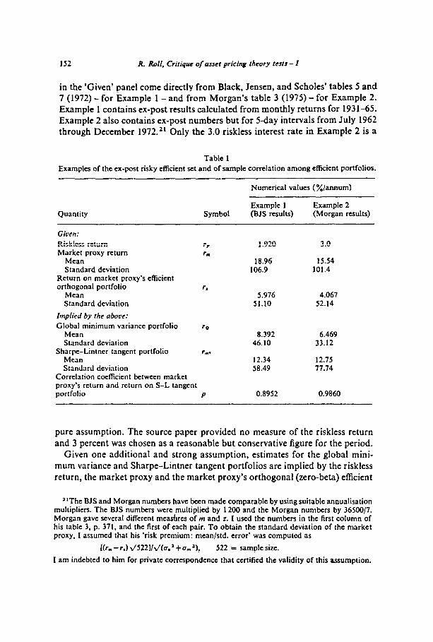
152 R. Roll, Critique of asset pricing theory tests - I
in the ‘Given’ panel come directly from Black, Jensen, and Scholes’ tables 5 and 7 (1972) - for Example 1 - and from Morgan’s table 3 (1975) - for Example 2. Example 1 contains ex-post results calculated from monthly returns for 1931-65. Example 2 also contains ex-post numbers but for 5-day intervals from July 1962 through December 1972. ‘l Only the 3.0 riskless interest rate in Example 2 is a
Table 1
Examples of the cx-post risky efficient set and of sample correlation among efficient portfolios.
Numerical values (%/annum)
Quantity Symbol Example 1 Example 2 (BJS results) (Morgan results)
Given: Riskless return Market proxy return
Mean Standard deviation
Return on market proxy’s efficient orthogonal portfolio
Mean Standard deviation
Implied by the above: Global minimum variance portfolio r0
Mean Standard deviation
Sharpc-Lintncr tangent portfolio rn. Mean Standard deviation
Correlation coefRcient between market proxy’s rclurn and return on S-L tangent portfolio P
1.920
18.96 106.9
5.976 4.067 51.10 52.14
8.392 6.469 46.10 33.12
12.34 12.75 58.49 17.74
0.8952 0.9860
3.0
15.54 101.4
pure assumption. The source paper provided no measure of the riskless return and 3 percent was chosen as a reasonable but conservative figure for the period.
Given one additional and strong assumption, estimates for the global mini- mum variance and Sharpe-Lintner tangent portfolios are implied by the riskless return, the market proxy and the market proxy’s orthogonal (zero-beta) efficient
lIThe BJS and Morgan numbers have been made comparable by using suitable annualisation multipliers. The BJS numbers were multiplied by 1200 and the Morgan numbers by 36500/7. Morgan gave several diKerent mea&es of m and I. I used the numbers in the first column of his table 3. p. 371. and the first of each pair. To obtain the standard deviation of the market proxy, I assumed that his ‘risk premium: mean/std. error’ was computed as
Nm - r.)\/5221/~/(a.‘+a,‘), 522 = samplesize.
I am indebted to him for private correspondence that certified the validity of this assumption.
R. Roll, Critique of asset pricing theory tests - I 153
portfolio that were provided in the source papers. The crucial assumption is that the market proxy and its associated zero-beta portfolio are actually located on the ex-post efficient frontier. ” If m and z are both efficient, the variance of each one is related to its mean by the efficient set quadratic equation, (A.ll) of the appendix, which contains the three ‘efficient set constants’, a, b and c. In addition, since m and z were orthogonal by construction, their means are related by a third expression (A.15) which is the general equation relating the mean returns of orthogonal efficient portfolios. Since this expression also con- tains the e5cient set constants, there results a non-linear system of three equa- tions in the three unknowns, (I, b and c. Usually, as in the case of our examples here, the system has a unique solution. Once the three efficient set constants are determined, all the other information of table 1 is computable in a straight- forward way. The Sharpe-Lintner tangent portfolio’s return requires addition- ally that the riskless interest rate be assigned a value.
The examples’ relevance derives from the tangent portfolio and its correlation with the proxy market portfolio. In Example 1, Black, Jensen, and Scholes’ data indicate that the Sharpe-Lintner tangent portfolio had an average monthly return of 12.3 (percent per annum) from 1931-65 and that its ex-post correlation with their market proxy was on the order of 90 percent. Notice that the tangent return was only 65 percent of the market proxy return, despite the significant correlation. Also note that the Black, Jensen, and Scholes zero-beta proxy re- turned 5.976 (percent per annum) on average. As mentioned previously, this finding was used by them to deny the validity of Sharpe-Lintner theory (because 5.976 was significantly greater than 1.920, the estimated riskless return).
There is a possible way to examine the validity of their conclusion. Using the same data, a different consistency check of the Sharpe-Lintner model would involve the individual asset investment proportions in the observed tangency portfolio. If any of these were significantly negative, the tangency portfolio would not satisfy the qualities of a market portfolio, which must have positive investments in all assets. ” The suggested exercise (it has not yet been done by anyone, to my knowledge), has been termed a ‘consistency check’ rather than a ‘test’ of the Sharp+Lintner theory because of the many assets omitted from the Black, Jensen, and Scholes sample. The omission of even a single asset can in principle cause an observed tangency portfolio to alter in composition
**There are several reasons why this is a strong assumption and why the results of table 1 should only be considered as examples. In both the Black, Jensen, Scholes and the Morgan papers, the samples consisted only of equities. Thus, it is very unlikely that the market proxy was exactly mean-variance efficient. Even if the samples had included all assets. the zero-beta measured portfolios were probably not precisely on the ex-post mean-variance boundary because the full covariance matrix was never inverted to find the efficient set constants. For example, Morgan estimated the etlicient set by using a sample of 89 portfolios of 6 securities each (p. 365). This estimate of the efficient set would have differed, although perhaps in only a minor way, from the efficient set computed using the 534 (89 x 6) individual stocks.
“1 am indebted to Michael C. Jensen for suggesting this procedure.
154 R. Roll, Critique of asset pricing theory tests - I
from totally positive to some negative proportions. (The alteration is not merely an allocation of the former weight of the omitted asset to the remaining assets because the entire efficient set can change.) Nevertheless, the calculation would be worthwhile because it would at least provide an insight into the possibility of incorrect inferences arising from market proxy portfolio misspecification within the Black, Jensen, and Scholes universe of securities. Unfortunately, the calculation cannot be reported here because it requires the full sample covariance matrix and the sample mean return vector of individual assets. These are not in my possession.
The Morgan data, which cover a later periodthan the Black, Jensen,and Scholes data, imply an even higher correlation between the marketproxy and the Sharpe- Lintner ex-post tangency portfolios. This is due partly to a lower mean return of the market proxy and partly to a larger assumed riskless return which has caused the tangent portfolio to lie closer to the proxy. 24 However, the same qualitative conclusions obtain: Efficient portfolios are highly correlated and the Sharpe- Lintner thecry is consistent with the data and a mis-specified market index.
Recall that all efficient portfolios on the positively-sloped segment are posi- tively correlated. It is also true that the correlation increases with increasing mean returns of the two portfolios in question (holding constant the difference between their means). In the two numerical examples of table 1, for instance, all efficient portfolios with returns between 14 and 49 percent for Example 1 and with returns between 12 and 36 percent for Example 2 had squared cor- relations with the market proxy greater than 90 percent.
The implications of this are clear: Any hypothesis, such as Sharpe-Lintner, that makes a spccilic prediction about the position of the market portfolio, is likely to bc highly susceptible to a type II error-being rejected when it is true. IIcuristically, a small error in measuring the market’s composition can cause an error in testing the theory. The market proxy may be almost perfectly cor- rclatcd with the true market and yet a significant dilfcrence can emerge between the proxy zero-beta return and the true zero-beta return (or the risklcss return).
3.2. The gcneralixd ussct pricing rhcory case
For testing the Sharpc-Lintncr hypothesis (H.4), the identifiability of the market portfolio is a serious problem. For the more general asset pricing hypo- thesis (H.Z), it is perhaps even a more serious problem. For (l-1.4), we can at least get an idea of the conscqucnccs of a mis-specihed market portfolio by assuming that the proxy market is ellicicnt. Then, the ex-post tangent portfolio can be calculated as in the above examples and its return and reasonableness can be
2’Thc effect of the risk& rat assumption is easy to nssess. For an assumption of 2% rather than 3”/& the correlation bcrwecn market proxy and tnngcnt portfolio would ha\;c been 0.9587. For 47:. the correlation would have been 0.9999. Thus a considerable range of assump- tions for the risklcss rate would have given the same general impression.
R. Roil, Critique of asset pricing theory tests - I 155
judged against external criteria. For example, it might have been expected that the true market portfolio had less variance and less return than the Black, Jensen, and Scholes and the Morgan all-equities proxies, perhaps because equi- ties are more variable than the average asset. Or, if the all-equities proxies had been combined with bonds, human capital, and real estate in reasonable pro- portions, the resulting mixture might have been closer to the observed tangent portfolio. Naturally, such possibilities are mere conjectures. They are not test- able hypotheses, again for the simple reason that the true market portfolio has an unknown composition.
For the more general hypothesis (H.2), such judgements based on common- sense interpretation of the results are likely to be unavailable. (H.2) merely requires that the true market be somewhere on the positively-sloped segment of the mean-variance efficient frontier. For relatively small (time-series) sample sizes, this hypothesis is highly susceptible to a type I error, being acceptable when it is false; but as the number of time-series observations increases, the hypothesis will almost surely be rejected, even when it is true. To see why, first consider the fact that the true market portfolio has a positive proportion invested in every individual asset. This implies that every reasonable candidate for the market proxy must have totally positive investment proportions. In many cases, in fact, the investment proportions are either the positive constant I/N for the included assets (and zero for excluded assets), or the proportions display little cross-sectional variation. We know, therefore, that all such candidates for the proxy market portfolio must lie in a relatively small region of the mean-variance space.
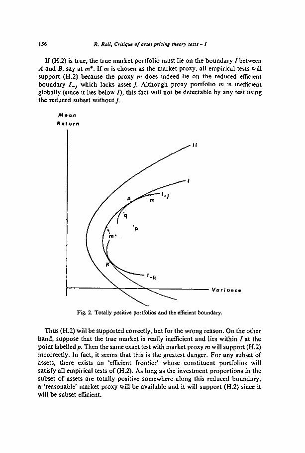
Suppose, for example, that the true eflicicnt set is given by the curve lab&d ‘I’ in fig. 2. In this particular example, cfficicnt portfolios bctwccn A and B arc assumed to have totally positive investment proportions. As shown in the appendix, Theorem 3, an efficient set like I, whose global minimum variance
portfolio has totally positive investment proportions, will occur if the variance of every individual asset exceeds its covariances with all other individual assets (if ui > o,, for alli # i). Above the point n and below the point B, at least
one asset has negative investment proportions. Suppose the asset that leaves the efficient set at point A is indexedj. Then the curve I_, would be the efhcient set ifj did not exist. /and I_, are tangent at a single point at most. (There might have been no finite tangency becausej might have had a positive or a negative
weight in all portfolios on I.) ” But since the weight is assumed negative above A and positive below A, it must be zero at A. Since it is zero everywhere on I_,, A must be a tangency. (, and I_, obviously cannot cross since they are minima.)
“The curve I_ ,, with one omitted asset, is olked as an expositional example. In general, thcrc will be more than one omitted asset from any empirical sample and so there will bc no common point bctwecn the true efficient frontier and the sample efficient frontier, except in an unusual circumstance (the unusual circumstance being that all omitted assets have their zero investment proportions at a common point on the true efficient set).
156 R. Roll, Critique of asset pricing theory tests - I
If (H.2) is true, the true market portfolio must lie on the boundary I between A and B, say at m*. If m is chosen as the market proxy, all empirical tests will support (H.2) because the proxy m does indeed lie on the reduced efficient boundary I_, which lacks asset j_ Although proxy portfolio m is inefficient globally (since it lies below I), this fact will not be detectable by any test using the reduced subset without j.
Mean
Roturn
Variance
Fig. 2. Totally positive portfolios and the efficient boundary.
Thus (H.2) will be supported correctly, but for the wrong reason. On the other hand, suppose that the true market is really inefficient and lies within Z at the point labelledp. Then the same exact test with market proxy m will support (H.2) incorrectly. In fact, it seems that this is the greatest danger. For any subset of assets, there exists an ‘efficient frontier’ whose constituent portfolios will satisfy all empirical tests of (H.2). As long as the investment proportions in the subset of assets are totally positive somewhere along this reduced boundary, a ‘reasonable’ market proxy will be available and it will support (H.2) since it will be subset efficient.
R. Roll. Critique of asset pricing theory tests - I 157
On the other hand, the geometry makes evident that a type II error is also quite possible. Suppose that portfolio q has been chosen as the market proxy and that (H.2) is true and that m* is truly e5cient and lies on I. In this case, a large sample will almost surely reject (H.2) since the proxy does not even lie on the reduced efficient set I_,. Note that this will occur even when the proxy is highly correlated with the true market m* and is also highly correlated with a proxy which is subset efficient.
The empirical situation is aggravated by this likelihood of a high correlation between the true market and the proxy, whether (H.2) is true or false. Such a high correlation is bound to make it seem that the exact identity of the market is of relatively minor significance and the temptation will be great to modify the market proxy slightly to obtain the desired result, whether it be rejection or acceptance of (H.2). In fact, if the identity of the true market is a matter of dis- pute among different researchers, there may be no way to settle the validity of (H.2) with any size of sample. The only exception would seem to be when (H.2) is false, the true state of nature is depicted by efficient set II in fig. 2 and the sample contains every asset. In this case, no totally-positive portfolio is efficient and large (time-series) samples would reject (H.2) unambiguously.
In principle, such a test is easy to construct. As shown in the appendix, the investment proportions for portfolios that lie on the ex-post e5cient boundary are given by the N x 1 vector
X-B ; ) 0 where B is an (Nx 2) matrix of constants that depend only on the mean returns and sample covariances of the N individual assets, and r is the mean return of the ex-post efficient portfolio whose investment proportions are given by X. Since B contains constants, the test simply involves computing X at two points - at the minimum and maximum observed individual returns, rmln and r,,, to obtain
and X,,,,, E B .
Then if there is a single element that is significantly negative in both X,,,,,, and X m.rr (H.2) is false. This follows because every totally positive portfolio lies between r,,,{, and r,,,.,. Thus, if all efficient portfolios in this interval have one or more significantly negative investment proportions, there is no totally positive mean-variance efficient portfolio. Unfortunately, this ‘test’ is only valid in principle. The full covariance matrix of all individual assets is required to compute the matrix B. Furthermore, the sampling variation of B would generally
158 R. Roll, Critique of asset pricing theory rests - I
be unknown. Finally, the cost of collecting data for etlery existing asset would be nrohibitive.
In summary of this section, the sole viable hypothesis of generalized asset pricing theory is (H.2) - the true market portfolio is ex-ante efficient. This hypothesis offers a non-trivial challenge to our econometric ingenuity and the challenge has not yet been satisfactorily met. The problem can be summarised by noting that in a given sample there are always portfolios which do not reject (H.2) and that little external information is available on the true market port- folio’s exact composition. Furthermore, even a small mis-specification of the proxy’s composition can lead to the wrong conclusion. What might seem a trivial mis-specification in an ordinary statistical application can be of crucial importance for testing (H.2).
Appendix
The eficient set mathematics2 6
The efficient set (or etlicient portfolio frontier) is composed of portfolios with minimum variance at each possible level of mean return. Ex-ante variances and mean returns of individual assets must be estimated or subjectively deter- mined. The ex-post ellicicnt set is a sample statistic, the set of minimum sample variance portfolios.
Given the characteristics of individual assets, a portfolio is completely charac- ter&d by the proportions invested in its constituent securities,
where xiP is the proportion of portfolio p invested in asset i, and X, is a vector subject to the constraint
XJ = 1, (A.0
I denoting the unit vector. When speaking of a single portfolio, we will suppress the subscript p on the vector X.
The parameters of the efficient set problem are the mean return vector of individual assets,
R = Ilr,ll,
26As mentioned in the text, most of the results in this appendix have appeared previously. See particularly Merton (1972). which is the original full analytic treatment of the efficient set mathematics. SzegG (1975) seems to be the only other relatively complete treatment but Sharpe (1970). Black (1972) and Fama (1976) also contain many of the same results. I have made no attempt to ascribe originality.
R. Roll, Critique of asset pricing theory tesfs - I I59
and the covariance matrix of individual returns,
These can be either population values or they can be sample product moments. The mathematics that follows does not require a distinction, merely a set of numbers R and V. Any portfolio’s mean and variance are given by
rP = X’R,
c7; = X’ vx.
Similarly, the covariance of any
by
0 PIP2
= x;,vx,,.
(A.21
(A.3)
two arbitrary portfolios (say p1 and pZ) is given
(A-4)
Necessary and su$icient condition for a portfolio to be eficient
The efficient set is found by minimizing ui subject to the two constraints (A.1) and (A.2). The Lagrangian is
L = X’VX-A,(X’R-rp)-J.2(X’I-1),
where AI and AZ are undetermined multipliers. The first extremum conditions are the vector
VX = f(l,R+&~),
plus the constraints (A. I) and (A.2).
(A.3
If the joint distribution of individual returns is non-degenerate, the covariancc matrix is positive definite (and non-singular), and all efftcient portfolios satisfy
X = f V-’ (RI) 4
0 ~ .
2 (A.6)
Non-degeneracy simply implies that no two distinct linear combinations of assets are perfectly correlated and that no asset has zero variance. We shall see later how to find the effkient set when this condition is not satisfied. When the probability distribution is non-degenerate, the second-order conditions for a minimum are satisfied because the covariance matrix is positive definite.
The equation of the eficient set
Different efficient portfolios are determined by different values of the multi- pliers in eq. (A.6). The result can be written in a more intuitive way, however, as shown in the following:
JFE B
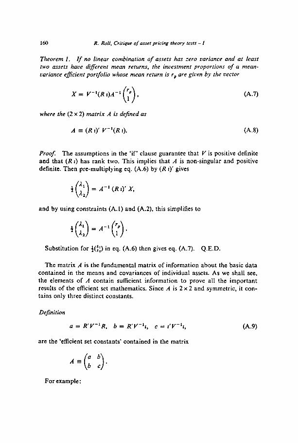
160 R. Roll, Critique of asset pricing theory WSIS - I
Theorem I. If no linear combination of assets has :ero variance and at least
two assets have different mean returns, the incestment proportions of a mean-
cariance ejicient portfolio whose mean return is r,, are gicen by the cector
X= V-‘(R I)A-’ ; , 0
where the (2 x 2) matrix A is defined as
A = (R 1)’ V-‘(R I). (A.8)
Boo/: The assumptions in the ‘if’ clause guarantee that V is positive definite aod that (RI) has rank two. This implies that A is non-singular and positive definite. Then pre-multiplying eq. (A.6) by (R I)’ gives
= A-’ (R I)’ X,
and by using constraints (A.l) and (A.2), this simplifies to
+(;j = A-‘(;).
Substitution for j(i:) in eq. (A.6) then gives eq. (A.7). Q.E.D.
The matrix A is the fundamental matrix of information about the basic data contained in the means and covariances of individual assets. As we shall see, the elements of A contain sufficient information to prove all the important results of the cfftcient set mathematics. Since A is 2 x 2 and symmetric, it con- tains only three distinct constants.
Definition
a = R’V-‘R, b = R’V-‘1, c = CV-‘l,
are the ‘efficient set constants’ contained in the matrix
(A.9)
For example:
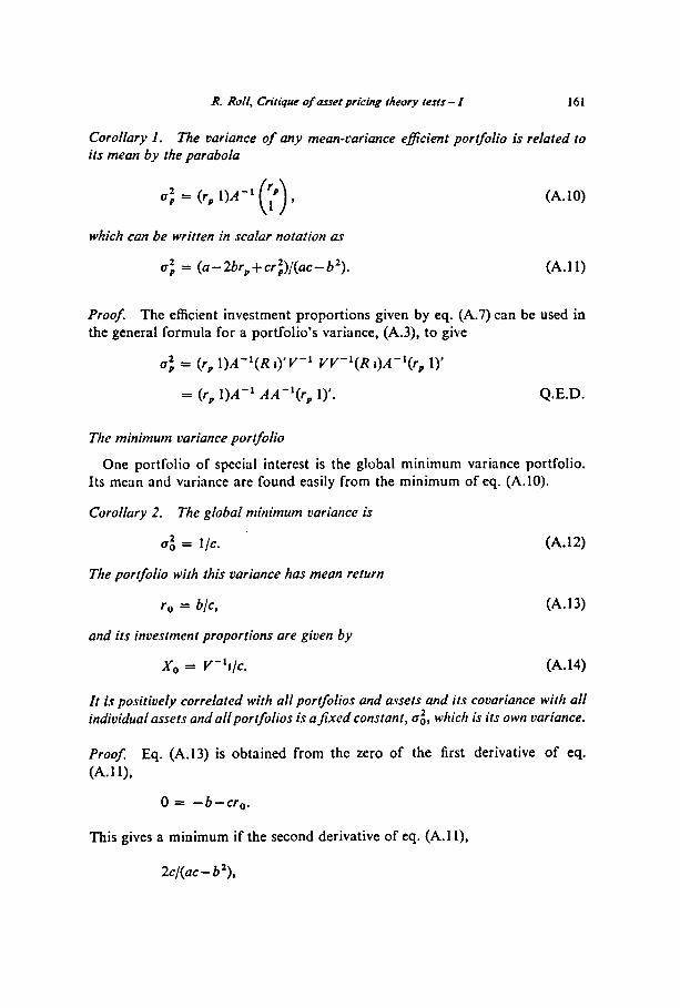
R. Roll, Critique of asset pricing rheory tests - I 161
CoroNary I. The variance of any mean-variance eficient portfolio is related to its mean by the parabola
17: = (rp l)A-’ F , 0
which can be written in scalar notation as
u’, = (a-2br,+cri)/(ac-b’). (A.1 1)
Proof. The efficient investment proportions given by eq. (A.7) can be used in the general formula for a portfolio’s variance, (A.3), to give
~7: = (rp l)A”(R [)‘Y-’ VY-‘(R l)A-‘(r, 1)’
= (rp l)A-’ AA-‘(r, 1)‘. Q.E.D.
The minimum variance portfolio
One portfolio of special interest is the global minimum variance portfolio. Its mean and variance are found easily from the minimum of eq. (A.lO).
Corollary 2. The global minimum variance is
a: = l/c. (A.12)
The portfolio with this variance has mean return
r. = b/c, (A.13)
and its investment proportions are given by
x0 = v-+/c. (A.14)
It is positively correlated with all portfolios and assets and its covariance with all individual assets and all portfolios is a fixed constant, ai, which is its own variance.
Proof. Eq. (A.13) is obtained from the zero of the first derivative of eq.
(A.1 l),
0 = -b-cr,.
This gives a minimum if the second derivative of eq. (A.1 l),
Zc/(ac - b 2),
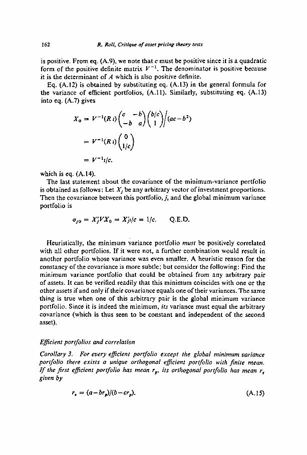
162 R. Roll, Critique of asset pricing theory tests
is positive. From eq. (A.9). we note that c must be positive since it is a quadratic form of the positive definite matrix V -I. The denominator is positive because it is the determinant of A which is also positive definite.
Eq. (A.12) is obtained by substituting eq. (A.13) in the general formula for the variance of e5cient portfolios, (A.1 1). Similarly, substituting eq. (A.13) into eq. (A.7) gives
which is eq. (A.14). The last statement about the covariance of the minimum-variance portfolio
is obtained as follows: Let X, be any arbitrary vector of investment proportions. Then the covariance between this portfolio,j, and the global minimum variance portfolio is
=JO = x;vxo = x;qc = l/c. Q.E.D.
Heuristically, the minimum variance portfolio nturt be positively correlated with all other portfolios. If it were not, a further combination would result in another portfolio whose variance was even smaller. A heuristic reason for the constancy of the covariance is more subtle: but consider the following: Find the minimum variance portfolio that could be obtained from any arbitrary pair of assets. It can be verified readily that this minimum coincides with one or the other assets if and only if their covariance equals one of their variances. The same thing is true when one of this arbitrary pair is the global minimum variance portfolio. Since it is indeed the minimum, its variance must equal the arbitrary covariance (which is thus seen to be constant and independent of the second asset).
Eficient portfolios and correlation
Corollary 3. For every eficient portfolio except the global minimum variance portfolio there exists a unique orthogonal efficient portfolio with finite mean. If the first efficient portfolio has mean rP, its orthogonal portfolio has mean r, given by
r, = (a - br,)/(b - cr,). (A.15)
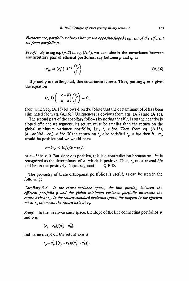
R. Roll, Critique of asset pricing theory tests - I 163
Furthermore, portfolio z always lies on the opposite-sloped segment of the eficient set from portfobo p.
Proof. By using eq. (A.7) in eq. (A.4), we can obtain the covariance between any arbitrary pair of e5cient portfolios, say between p and q, as
uqp = (r,l) A-’ ‘;9 . 0
(A.16)
If p and q are orthogonal, this covariance is zero. Thus, putting q = z gives the equation
(rr 1)(_;_3(:) = 0,
from which eq. (A.15) follows directly. [Note that the determinant of A has been eliminated from eq. (A.16).] Uniqueness is obvious from eqs. (A.7) and (A.15).
The second part of the corollary follows by noting that if r, is on thenegatively sloped efficient set segment, its return must be smaller than the return on the global minimum variance portfolio, i.e., r, < b/c. Then from eq. (A.15), (a- br,)/(b- cr,,) < b/c. If the return on r,, also satisfied r,, < b/c then b-err would be positive and we would have
a - br, < (b/c)(b - err),
or a-6*/c c 0. But since c is positive, this is a contradiction because ac-b* is recognized as the determinant of A, which is positive. Thus, rr must exceed b/c and be on the positively-sloped segment. Q.E.D.
The geometry of these orthogonal portfolios is useful, as can be seen in the following:
Corollary 3.A. In the return-variance space, the line passing between the eficient portfolio p and the global minimum variance portfolio intersects the return axis at r,. In the return-standard deviation space, the tangent to the e&ient set at rr intersects the return axis at r,.
Proof In the mean-variance space, the slope of the line connecting portfolios p and G is
(‘P - re)/(a2, - c3,
and its intercept on the return axis is
164 R. Roll. Crilique of usset pricing rheory fesls - I
Substituting for r0 and 0: from eqs. (A.13) and (A.12) and simplifying, this expression reduces to (br,-a)/(~,-b) which is rz in eq. (A.1 5). Thus the first statement is proven. To prove the second, it is easiest to use the first derivative of eq. (A.1 1). This provides an expression for the tangent to the efficient set in the mean-standard derivation space. Multiplying this tangent by bP and sub- tracting the result from r,, gives eq. (A.15). Q.E.D.
Corollary 4. All portfolios on the positively-sloped segment of the eficient set are positively correlated.
ProoJ From eq. (A.16) we can see that any two efficient portfolios, p and q, will be negatively correlated if and only if
a-b(r,+rJ+c rprrl < 0,
which ivplies that
a- br, < r&b-crp).
If p is on the positively-sloped efficient segment, b - crp < 0, and thus r* < r,, where z is p’s orthogonal portfolio. But z must lie on the negatively-sloped segment, from Corollary 3. Thus, q is also on the negatively-sloped segment since its return is smaller than rr. Q.E.D.
It is easy to see by the same argument that all portfolios on the negatively- sloped segment arc positively correlated too. Only portfolios that lie sufficiently far apart, and on opposite sides of the efficient set, are negatively correlated. Heuristically, if investors do wish to minimize variance and maximize expected returns, all investors who agree on the probability distribution would hold positively correlated portfolios.
The separation or ‘two-fund’ theorem
Corollary 5 (‘Two-Fund Theorem’). The investment proportions vector of every mean-variance eficient portfolio is a linear combination of the proportions vector: of two other eficient portfolios whose means are diflerent.
Proof. From eq. (A.7). the investment proportions are seen to be linear in the mean return. This is so because the (Nx 2) matrix, B E V-‘(R I)A”, contains only constants (N is the number of individual assets). Thus, if pl, p2 and p, are efficient portfolios and a is a constant given by a = (r3 - rJ/(rI - rl),
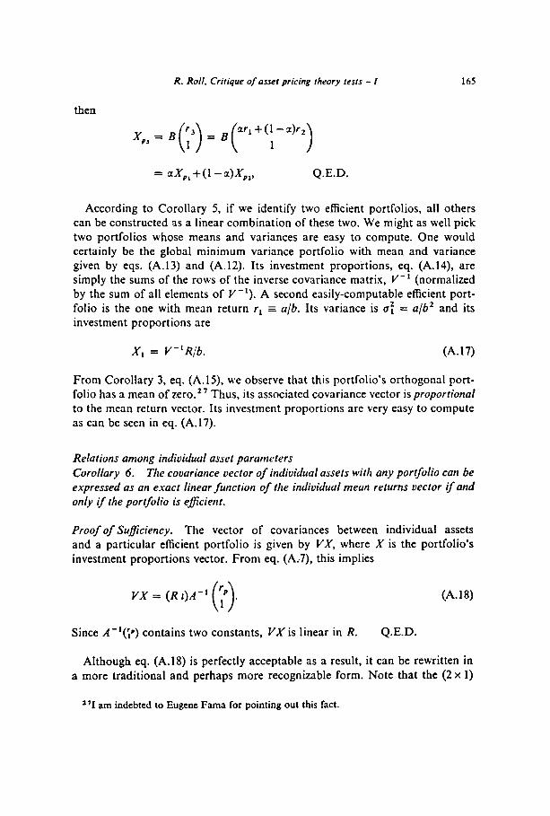
R. Roll, Critique of asset pricing rheory tests - I 165
then
cxr,+(l-z)rz
1
= ax,, +(l -a)XPI, Q.E.D.
According to Corollary 5, if we identify two efficient portfolios, all others can be constructed as a linear combination of these two. We might as well pick two portfolios whose means and variances are easy to compute. One would certainly be the global minimum variance portfolio with mean and variance given by eqs. (A.13) and (A. 12). Its investment proportions, eq. (A.14), are simply the sums of the rows of the inverse covariance matrix, Y-’ (normalized by the sum of all elements of V-‘). A second easily-computable efficient port- folio is the one with mean return rl - a/b. Its variance is 0: = a/b* and its investment proportions are
X, = V-‘R/b. (A.17)
From Corollary 3, eq. (A.15). we observe that this portfolio’s orthogonal port- folio has a mean of zero.” Thus, its associated covariance vector is proportional to the mean return vector. Its investment proportions are very easy to compute as can bc seen in eq. (A.17).
Relations among individual asset parameters Corollary 6. The covariance vector of individual assets with any portfolio can be expressed as an exact linear function of the individual mean returns vector if and only if the portfolio is eficient.
Proof of Suficiency. The vector of covariances between individual assets and a particular efficient portfolio is given by VX, where X is the portfolio’s investment proportions vector, From eq. (A..7), this implies
VX= (R&4-’ ;p . 0
(A.18)
Since A-‘(y) contains two constants, VX is linear in R. Q.E.D.
Although eq. (A.18) is perfectly acceptable as a result, it can be rewritten in
a more traditional and perhaps more recognizable form. Note that the (2 x 1)
2’I am indebted to Eugene Fama for pointing out this fact.
166 R. Roll, Critique of asset pricing theory tests - I
vector A-‘(y) can be simplified as
where z is p’s orthogonal portfolio. Substitution back into eq. (A.18) gives
R = rzl+(rp-rz)B, (A.19)
where j3 E KY/u’, is the vector of simple regression slope coefficients of indivi- dual assets on efficient portfolio p (the ‘betas’). Since the covariances are linear in the mean return, of course the ‘betas’ are too.
Proof of Necessity. Let the vector of covariances with an arbitrary portfolio m be an exact linear function of the mean returns,
vx, = a,R+a,l,
where a, and a2 are arbitrary constants. Then the vector X,,, is equal to
X” = a,V”R+a,V-‘r
= albX, +a,cX,,,
where X, is the vector of investment proportions for special efficient portfolio 1 [WC cq. (A.l7)], and X0 is the vector of proportions for the global minimum variance portfolio (b and c are two of the three efficient set constants).
Since the constraint (A.l) must apply to all such vectors, including the vector X,,,, we must have
a,b+a,c = 1.
Thus X,,, is a weighted average of two efficient vectors X, and X0 and, by Corollary 5, X, also is efficient. Q.E.D.
A slightly more general form of the linearity property can be obtained. Let us suppose that portfolios A and B are chosen arbitrarily and that the multioariate regression coefficients are computed between individual asset returns and these two portfolios’ returns. Then:
Corollary 6.A. 28 Let vectors of m~rltivariate regression coeflcients be calcu- lated between individual asset returns (as dependent variables) and the returns o
*‘I am indebted to John B. Long. Jr. for pointing out a previous error in this corollary.
R. Roll. Critique of ossel pricing theory tests - I 167
two imperfectl~correlated portfolios A and B (as explanatory variables). Then both multivariate regression coeficient vectors are exact linear functions of the mean return vector if and only if A and B are eficient. Furthermore,
(a) the coeficient vector for asset j on portfolio A is given by
(V-G - a,&/(aj - bAB) = (R - rel)/(r,, - rB), (A.20)
and similarly for portfolio B with the A and B subscripts interchanged; and (b) the two coeficient vectors sum to the unit vector.
Proof of Suflciency. If statement (a) is true, the proof of exact linearity is identical to the proof of Corollary 6 because (A.20) shows that the multivariate coefficient vector is linear in the covariance vector VX,. Since a linear function of a linear function is also linear, the result follows immediately.
To prove parts (a) and (b), first note that the usual multivariate coefficient of A obtained by regressing j on A and B would have been
But since A and B are mean-variance efficient, this multivariate coefficient can be simplified. Noting from eq. (A.19) that c]B = &(r,-rz,,)/(rg-rz,), where zB is B’s orthogonal portfolio, and noting analogous expressions for ojA and Q,,~, eq. (A.21) can bc rewritten as
or
P; =
P; =
(r,-rrJ(rB-rzo)-(r,-rzs)(rB-rrl)
(rA - r,,)(r~ -rrJ-(rA-rzs)(rB-rJ’
rJ - rE =jA - =A5
-=z* rABrB =A -=AB
(A.22)
This proves part (a). Since the same development can be made in behalf of portfolio B, the multivariate coeffkient against B must be (r,-r,,)/(~~-rA) = 1 -pi. This proves part (b). Q.E.D.
Proof of Necessity. Let both multivariate coefficient vectors be exact linear functions of the mean return vector. Using the general definition (A.21) of multivariate coefficients and the same procedure as that contained in the neces- sity proof of Corollary 6, it can be shown that the vectors W, and W,, defined
by
168 R. Roll, Critique of asset pricing theory tests - I
and
are efficient. (Here, jAB = Q,&;.) Adding the two equations in order to eliminate X, gives
Since the coefficients of W, and W, sum to 1 -~BAfiAB, X, is a linear combina- tion of two efficient vectors and is therefore also efficient (by Corollary 5). An identical development proves the efficiency of vector X,. Since A and B are efficient, statements (a) and (b) are true. Q.E.D.
Suppose that some non-efficient portfolio q has been used to estimate a vector of betas. There exists an efficient portfolio p that has the same mean return,
TP = r , and for which eq. (A.19) is satisfied. But the betas of eq. (A.19) are
VXp/afp whereas the betas estimated with portfolio q are fl = VXJui. Using the estimates fl, (A.19) can be rewritten as
R E rr + (r(- r,)fl + r+ F’(X,/k - X,), aq
(A.23)
where k = u:/u,‘. The expression (A.23) is linear in the vector fl if and only if the last term is a constant vector. But ifq is not efficient, then k < 1. This implies that the last term can be constant only if rp # rq, which is a contradiction. (This is actually an equivalent proof to that used for Corollary 6; but it has the advantage that the deviations from a linear return-beta relation caused by using an inefficient base portfolio are given explicit display.)
One featureof eq. (A.23) is of particular interest: It would be quite possible that a subset of the elements of Xp and X, be equal; and if the returns and betas for this particular subset were calculated, they would be exactly linearly related when taken alone. Thus the full set:of data is not conrinuou.sl_~ non-linear even when the base portfolio is inefficient.
To reiterate, an efficient set calculated from a subset of assets will pass through portfolios that are inefficient globally. But since such portfolios are efficient for the subset, their associated subset of betas will be exactly linear in the subset of mean returns.
Corollary 7. The proportion invested in a given individual asset changes monotonically along the eficient frontier.
Proof. By inspection from eq. (A.7). (The gradient vector of X with respect to rp is a constant vector.)
R. Roll. Crifique of asset pricing theory tests - I 169
This corollary implies that if an individual asset represents a non-zero pro- portion in any efficient portfolio, it is held in of/efficient portfolios except at most one. It is either held in positive amount or sold short in all others. N.B. It is mathematically possible that some assets are positively (or negatively) rep- resented in all efficient portfolios and even that the individual proportion is a constant.
The gradient vector of eq. (A.7) can be written as
8 X/Jr, = a$-‘(R/r,, -t)/(rl -r,,), (A.24)
where rl and r,, are means of, respectively, the special efficient portfolio 1 (see Corollary 5), and of the global minimum variance portfolio. ai is the global minimum variance. The gradient vector of the covariance between individual assets and efficient portfolios is a(VX)/& and thus it is also monotonic. Since rr > r,-, if r,, is positive, we see that as the efficient portfolio’s return increases, the covariance between a given asset and the portfolio increases (is zero, or decreases) when the asset’s mean return is larger (equal to, or smaller) than the return on the global minimum v.ariance portfolio.
In contrast, the betas computed with efficient portfolios are not monotonic. In fact:
Corollary 7.A. To every individual asset, there corresponds a unique pair of orthogonal portfolios which provides the maximum and minimum betas for that asset. These portfolios have returns
r = rx,f~~~z, &I, (A.23
where 2, is the eficient portfolio whose return is orthogonal to the return of asset j, ai is the globul minimum variance, and A is the eficient set information matrix (A.8).
Proof. The beta of any individual asset with efficient portfolio p is given by
/I, = (r, l)A-‘(r, I)‘/+ (A.26)
Differentiating with respect to rP gives a function whose zero is a quadratic equation in rp. Some tedious algebra simplifies the result to (A.25). (Note that 0: is a function of rp.)
To prove that the maximum and minimum beta eficicnt portfolios are orthogonal, simply use (A.4). Their covariance is
(r,+K i)A-‘(r,-K l)‘,
170 R. Roll, Critique of asset pricing theory tests - I
In scalar notation, this reduces to
(a - 2br,, + a,: - cK2)/lA [,
and since
t7 Z, = (a-2brz,+cr,2,)/lAl = cK2/lA(,
the covariance is zero. Q.E.D.
An asset whose return is greater than the return on the minimum variance port- folio will be positively correlated with all efficient portfolios on the positive segment. This implies that its maximum-beta efficient portfolio will have return rz,+aOa,, @I, and its minimum-beta efficient portfolio will have return equal to the smaller root of eq. (A.25).29
A straightforward application of I’Hapitals’ rule to eq. (A.26) shows that every individual beta converges to zero as the efficient portfolio’s return grows indefinitely large (or small). (This does not violate the fact that the weighted average beta is always one because the investment proportions grow indefinitely large in absolute value.) As an implication, the cross-sectional variance in beta is determined by the particular efficient portfolio used in the computation. When the global minimum variance portfolio is used, all betas are equal to I.0 and their cross-sectional variance is zero. At an infinite return, all betas con- verge to zero and again their cross-sectional variance is zero. Naturally, there must exist an efficient portfolio whose associated betas have a maximum cross- sectional variation :
Corollary 7.8. The_ maximum cross-sectional variance in beta is given by eirher one of the two eflcientportfolios whose returns are
rP = r,+ai JIAI, (A.27)
where r,, and c$ are the mean and variance of the global minimum variance port- folio and A is the e#cient set information matrix (A.8).
3vAs an example, for the Black, Jensen, and Scholes data of table 1 in the paper, an asset with the same return as the proxy market, r, = 18.96 percent, would have had a maximum beta of 1.66 and a minimum of -0.659 over all efficient portfolios. (Assuming that the BJS market proxy and its zero beta portfolio were in fact etlicicnt.) The two ct?icient pdrtfolios that would have provided these maximum and minimum betas had returns of 11.6 and 0.375 percent, respectively.
R. Roll. Critique of asset pricing theory fests - I 171
Proof. It is possible to prove this result directly from the definition of beta, but the algebra is tedious. A shorter proof uses the fact that all beta vectors computed for efficient portfolios are exactly linear in the mean return vector (see Corollary 6). From the linearity relation (A.19), we must have
B = CR - v)l(rp - rz), (A.28)
and the cross-sectional variance in beta is therefore
Var (B) = Var (R>/(r,-rZ)2. (A.29)
The cross-sectional variance of individual returns, Var (R), is a constant with respect to movements along the efficient set. Thus, Var (/I) is maximized when IrP-rZl is minimized. From Corollary 3, we note that r, is a simple function of rP [eq. (A.15)]. The first derivative of rp-rr with respect to r,, gives a quadratic equation in rp whose solution is eq. (A.27). Q.E.D.
It is evident that the two portfolios which satisfy eq. (A.27) lie symmetrically on oppositely-sloped segments of the efficient frontier. The elements of their two associated beta vectors must therefore be equal and of opposite sign.30 They are also orthogonal. These are the only orthogonal efficient portfolios whose variances are equal and by Corollary 3.A, their variance is 2ai.
The cficient set when the minimum variance is zero
A special problem arises when the lcast-risky portfolio has zero variance.” This could bc caused by the cxistcnce of a risklcss asset but the possibilities for its occurrence arc much broader. In gcncral, it occurs if the covariance matrix of returns is only positive semi-definite; that is, if there exists a vector of invest- ment proportions X, such that XLVX, = 0.
Since Y is no longer of full rank, its singularity precludes the direct calculation of the investment proportions vector. The simplest and most intuitive way to find them is to proceed in two steps as follows. First, find the efficient set para- bola for the restricted group composed of all mutually non-degenerate assets. This means that any non-risky assets and one member of each pair of perfectly- correlated assets must first be discarded. A ‘risky efficient set’ is constructed from the remaining assets. For example, if the original N assets had covariance
“Continuing the numerical example with the Black, Jensen and Scholes data (table I), the cfflcicnt portfolios with returns 13.44 and 3.44 percent would have maximized the cross- sectional beta variance.
“Mathematically speaking. there is nothing to preclude several zero-variance portfolios with dilTercnt mean returns. Of course rational asset pricing would preclude such an event since in the absence of restrictions on short-selling, an infinite return could be obtained without a risk.
172 R. Roll, Critique of asset pricing theory tests - I
matrix V with rank L c N, N-L rows and columns of V would be discarded to obtain an L x L covariance matrix, V,, with full rank. It is obvious that all the results found previously for V when it had rank N must apply to the restricted set o/L assets whose covariunce matrix is V,. In particular, Theorem 1 and Corol- laries l-7 all apply to the reduced space of L assets. A reduced ‘risky efficient set’ can be derived; the betas calculated against portfolios that lie on this ‘risky efficient set’ are linear in the reduced vector of mean returns. The minimum variance among portfolios of the L assets is l/r’V,_-‘I; and so on.
This implies :
Theorem 2. Let an efficient set be computedfrom the L assets whose covariance matrix is non-singular. Then the global eficient set is composed of
aX, = au; VL1[(RL - r&/(ro -m (A.30)
as investment proportions in the L assets and 1 - ar’X, in the zero-variance asset F. The scalar a is positive for eficicnt portfolios on the positive (negative) segment if rF is less (greater) than the return r,, on the minimum variance portfolio of the L assets. ai is this minimum variance.
Proof. Since the global minimum variance is zero, the efficient set is com- posed of line scgmcnts in the mean-standard deviation space. This means that there is some tangent to the reduced (L asset) mean-standard deviation efficient set which passes through rF and gives the global efficient set. From Corollary 324, we see that the return at the tangency point must be the solution to
rp = (br, - a)@, - b),
where a, b. and c arc the three ‘efhcicnt set constants’ for the L assets only. This equation is rcvcrsiblc, which implies
rr = (brF - a)/(crF - b).
Substituting rz in (A.7) gives the XL investment proportions vector used in (A.30).
The last part of the theorem is established by noting that
rF - r* = (a - 2br, + cr:)/(cr, - b).
The numerator is positive since lALl = ac-b2 > 0. Thus rr 5 rF implies rF 2 b/c = ro. Q.E.D.
An alternative proof proceeds directly from the variance of the reduced set
R. Roll, Critique of asset pricing theory tests - I 173
of efficient portfolios. In other words, we can find the minimum with respect to rr of
a2u2 P’
subject to
r = ar,+(l-a)r,.
Using the efficient set variance formula for af, the first derivative of a2ai is zero when
(‘P - rJ(crp - 6) - ((1 - 2brp + cr,‘) = 0,
and this reduces to
rp = (br, - u)/(crr - b).
Corollary. When V is singular, all positive-variance eficient portfolios are per/ectly correlated.
ProoJ Theorem 2 shows that the vector ax, of investments in the reduced L asset space is proportional for all positive variance efficient portfolios. The remaining investment, 1 -al’XL, is placed in a zero-variance asset. Thus, the returns on all efficient portfolios are exactly linearly related. Q.E.D.
Qualitative results for investment proportions vectors
The sign pattern of the investment proportions vector of an efficient portfolio is an important datum in several contexts. For example, the interdiction of short-selling would leave a region of the efficient frontier unchanged if and only if that region were characterized by totally non-negative investment proportions, x 1 0.
Perhaps more importantly, there may exist no efficient vector such that X > 0. This means that no efficient portfolio has positive investments in all individual assets; which would imply, in turn, that the ‘market’ portfolio (composed of all assets) could not be efficient. If the reader thinks there must be some efficient portfolio whose X vector is positive, the counter-example in the footnote is offered.32 There seems to be no necessary economic reason to con-
“Let three assets have mean return vector and covariancc matrix,
R’ = (1 2 3) and V = G : 19.
Using eq. (A.7). it can be verified readily that every efficient portfolio contains a zero investment in the second asset.
174 R. Roll. Critique of asset pricing theory tests - I
sider such examples pathological. In particular, the argument that such mean (anticipated) returns must be out of equilibrium presupposes that investors regard mean-variance efficiency as optimal.
When the global minimum variance is zero, the entire efficient set is composed of linear combinations of X, and XL (see Theorem 2 above). Suppose that F is a single riskless individual asset. Then we can restrict our attention to XL >( 0. When the global minimum variance is positive, things are slightly more compli- cated because a totally positive vector X might occur anywhere within the
range trm.X, fminl, i.e., between the maximum and minimum individual asset returns.
A beginning to this problem is suggested by the following:
Theorem 3 [ Debreu-Herstein (2953)]. Suppose the covariance matrix is non-negative. Then if the global minimum variance portfolio has totally positive investment proportions, the variance of every individual asset is larger than each of its associated covariances.
Proof. Suppose we put V -I = sl- Q. Where I is the (Nx N) identity matrix and Q > 0. Debreu and Herstein showed that V >= 0 if and only ifs is larger than the largest eigenvalue of Q. This implies that in the matrix sl- Q, all diagonal elements are positive and all off-diagonal elements are negative Furthermore, they also showed (p. 603). that if the sum of every row of sl- Q. is positive, and if d,, is the cofactor of its ith row andjth cohrmn, then d,, > drJ for all i # j [see also Quirk and Saposnik (1968, pp. 210-21 I)]. Q.E.D.
This result can be intcrpretcd as follows. The weights X, of the global mini- mum variance portfolio arc proportional to the sums of the rows of V-’ [see (A.14)]. Thus a necessary condition for X0 > 0 is that each of V’s diagonal elements exceeds every off-diagonal element in the same row. Heuristically, such a condition implies weak correlation among every pair of assets. For any pair, say i andj, we must have not only u:oj > a; (which is always satisfied when V is non-singular), but also of > a,, and uj > o,,. The minimal variance formed by every combination of two assets must bc associated with a positive investment in both assets. Viewed geometrically, the locus of portfolios formed from every pair of assets is bowed outward toward the return axis between them. It seems likely that this result can be generalized to the case when V contains some negative covariances but I have not been able to find a proof.
Since the global minimum variance portfolio has strictly positive proportions in this case, by Corollary 7 above there must be a finite range of efficient port- folios with strictly positive investment proportions in its neighborhood.
In fact, every efficient portfolio, whose return r,, satisfies
(R I)A-’ I;p > 0, 0
R. Roll, Critique of asset pricing theory tests - I 175
has a totally positive investment proportions vector [cf. Debreu and Herstein (1953, p. 601)]. This condition is equivalent to
(R-r&,-r,) > 0,
where r, is p’s orthogonal portfolio and 0 is the global minimum variance portfolio. From the geometry Corollary 3.A, it is easy to see that (R - rz~>(rp- r,J is strictly positive for some fP in rmin 5 rP 6 r,.,,_. Since in the present case the global minimum variance portfolio is totally positive, fmin < rc, < r,,,_, and there is a finite range where the vector is positive. If the covariance matrix satis- fies the conditions of Theorem 3, we must have the following bounds on ortho- gonal portfolios association with f,,,_ and rmrn:
Unfortunately, this result does not, constitute a necessary condition for the existence of some totally positive efficient proportions vector. Examples are easy to construct where the global minimum variance portfolio has negative investment proportions but where another efficient portfolio is totally positive. Typically, this would occur when r0 is outside the range [f,,,_, rmin] and when there are relatively strong positive correlations among individual assets. In other words, when there are certain assets whose variances are inferior to some of their associated covariances. It is only for sufficiently strong correlations that X becomes non-positive everywhere (as in the example of footnote 32).
Black, F., 1972, Capital market equilibrium with rcstrictcd borrowing. Journal of Business 45, 443454.
Black, F., M.C. Jcnscn and M. Scholcs, 1972. The capital asset pricing model: Some empirical tests, in: M.C. Jcnscn, cd., Studies in the theory of capital markets (Praeger. New York).
Blume, M.E. and 1. Friend, 1973, A new look at the capital asset pricing model. Journal of Finance 28. 19-34.
Cass. D. and J.G. Stiglitz. 1970. The structure of investor preference and asset returns, and separability in portfolio allocation: A contribution to the pure theory of mutual funds, Journal of Economic Theory 2. 122-l 60.
Debreu. G. and I.N. Herstein. 1953. Non-negative square matrices, Economctrica 21,597-607. Fama, E.F., 1976, Foundations of finance (Basic Books. New York). Fama, E.F. and J.D. MacBeth, 1973. Risk, return and equilibrium: Empirical tests, Journal of
Political Economy 81, 607-636. Fama. E.F. and J.D. MacBeth, 1974a. Long-term growth in a short-term market, Journal of
Finance 39. 857-885. Fame. E.F. and J.D. MacBcth, 1974b. Tests of the multi-period two-parameter model, Journal
of Financial Economics 1. 43-66. Fisher, L.. 1966. Some new stock market indices. Journal of Business 23. 191-225. Friend, I. and M. Blume. 1970. Measurement of portfolio performance under uncertainty.
American Economic Review 60. 561-575. Hakansson. N.H., 1969, Risk disposition and the separation property in portfolio sclcction.
Journal of Financial and Quantitative Analysis 4,401-416.
176 R. Roll, Critique of asset pricing theory tests - I
Jacob, N.. 1970. The measurement of market similarity for securities under uncertainty, Journal of Business 43. 328-340.
Jensen. M.C.. 1972a. Capital markets: Theory and evidence, Bell Journal of Economics and Management Science 3, 357-398.
Jensen, M.C., 1972b. The foundations and current state of capital market theory, in: M.C. Jensen, ed., Studies in the theory of capital markets (Praeger. New York).
Lintner. J.. 1965, The valuation of risk assets and the selection of risky investments in stock portfolios and capital budgets, Review of Economics and Statistics 47. 1347.
Liitner, J., 1969, The aggregation of investor’s diverse judgements and preferences in purely competitive security markets, Journal of Financial and Quantitative Analysis 4. 347-lOO.
Long, J.B., 1976, Mean-variance efficiency and portfolio choice in the context of differential taxation of dividends and capital gains, unpublished manuscript (Graduate School of Management, University of Rochester, NY).
L&e. J.F. and R. Brealey, 1972. Modem developments in investment management (Praeger, New York).
Mayers, D., 1973, Nonmarketable assets and the determination of capital asset prices in the absence of a riskless asset, Journal of Business 46, 258-267.
Merton, R.C.. 1972, An analytic derivation of the efficient portfolio frontier, Journal of Financial and Quantitative Analysis 7. 1851-1872.
Merton, R.C., 1973, An inter-temporal capital asset pricing model. Econometrica 41.867-887. Miller, M.H. and M. Scholes, 1972, Rates of return in relation to risk: A re-examination of
some recent findings, in: M.C. Jensen, ed., Studies in the theory of capital markets (Praeger, New York).
Modigliani. F., G. Pogue, M. Scholes and B. Solnik, 1972. Efficiency of European capital markets and comparison with the American market, Proceedings of the First International Conference on Stock Exchanges, CISMEC.
Morgan, I.G., 1975, Prediction of return with the minimum variance zero-beta portfolio, Journal of Financial Economics 2, 361-376.
Palacios, J., 1973, The stock market in Spain: Tests of efficiency and capital market theory, unpublished dissertation (Stanford University, CA).
Petit, R.R. and R. Westerfield. 1974. Using the capital asset pricing model and the market model to predict security returns, Journal of Financial and Quantitative Analysis 9. S79- 605.
Pirsig. R.M.. 1974. Zen and the art of motorcycle maintenance (William Morrow, New York). Quirk, J. and R. Saposnik. 1968. Introduction to general equilibrium theory and welfare
economics (McGraw-Hill, New York). Roll, R., 1973. Evidence on the ‘growth-optimum’ model. Journal of Finance 28, 551-566. Roll, R. and B.S. Solnik, 1975, A pure foreign exchange asset pricing model, Journal of Intcr-
national Economics (forthcoming). Rosa, J.J.. 1975, Rentabilite, risque et cquilibrc a la boursc de Paris, Working Paper 7508
(Institut OrlCanais de Finance). Ross, S.A.. 1972, The arbitrage theory of capital asset pricing, Working Paper 2-73 (Rodney
L. White Center for Financial Research, University of Pennsylvania, Philadelphia, PA), forthcoming in Econometrica.
Ross. S.A., 1973, Return. risk and arbitrage, Working Paper 17-73a (Rodney L. White Center for Financial Research, University of Pennsylvania, Philadelphia, PA).
Ross, S.A.. 1976, Mutual fund separation in financial theory -The separating distributions. Working Paper 1-76 (Rodney L. White Center for Financial Research, University of Pennsylvania, Philadelphia. PA).
Ross, S.A., forthcoming, A note on the capital asset pricing model (CAPM), short-selling restrictions, and related issues, Journal of Finance.
Sharpe, W.F., 1964. Capital asset prices: A theory of market equilibrium under conditions of risk, Journal of Finance 19.425-442.
Sharpe. W.F., 1970. Portfolio theory and capital markets, (McGraw-Hill, New York). SzegB, G.P., 1975, Nuovi risultati analitici nella teoria dclla selezione de1 portafoglio (C.N.R.,
Comitato Scicnze Economiche, Sociologiche c Statistiche).